IBM SPSS COMPLEX SAMPLES 19 User Manual

IBM SPSS Complex Samples 19

Note: Before using this information and the product it supports, read the general information under Notices on p. 267.

This document contains proprietary information of S PSS Inc, an IBM Company. It is provided under a license agreement and is protected by copyright law. The information contained in this publication does not include any product warranties, and any statements provided in this manual should not be interpreted as such.

When you send information to IBM or SPSS, you grant IBM and SPSS a nonexclusive right to use or distribute the information in any way it believes appropriate without incurring any obligationtoyou.

IBM® SPSS ® Statistics is a comprehensive system for analyzing data. The Complex Samples optional add-on module provides the additional analytic techniques described in this manual. The Complex Samples add-on module must be used with the SPSS Statistics Core system and is completely integrated into that system.

About SPSS Inc., an IBM Company

SPSS Inc., an IBM Company, is a leading global provider of predictive analytic software and solutions. The company’s complete portfolio of products — data collection, statistics, modeling and deployment — captures people’s attitudes and opinions, predicts outcomes of future customer interactions, and then acts on these insights by embedding analytics into business processes. SPSS Inc. solutions address interconnected business objectives across an entire organization by focusing on the convergence of analytics, IT architecture, and business processes. Commercial, government, and academic customers worldwide rely on SPSS Inc. technology as a competitive advantage in attracting, retaining, and growing customers, while reducing fraud and mitigating risk. SPSS Inc. was acquired by IBM in October 2009. For more information, visit http://www.spss.com.

Preface

Technical support

Technical support is available to maintenance cus Technical Support for assistance in using SPSS Inc. products or for installation help for one of the supported hardware environments. To reach Technical Support, see the SPSS Inc. web site at http://support.spss.com or ﬁ

http://support.spss.com/default.asp?refpage=contactus.asp. Be prepared to identify yourself, your

organization, and your support agreement when requesting assistance.

Customer Service

If you have any questions concerning your shipment or account, contact your local ofﬁce, listed on the Web site at http://www.spss.com/worldwide. Please have your serial number ready for identiﬁcation.

Training Seminars

SPSS Inc. provides both public and onsite training seminars. All seminars feature hands-on workshops. Seminars will be offered in major cities on a regular basis. For more information on these seminars, contact your local ofﬁce, listed on the Web site at http://www.spss.com/worldwide.

tomers. Customers may contact

nd your local ofﬁce via the web site at

iii

Additional Publications

The SPSS Statistics: Guide to Data Analysis, SPSS Statistics: Statistical Procedures Companion, and SPSS Statistics: Advanced Statistical Procedures Companion, written by Marija Norušis and published by Prentice Hall, are available as suggested supplemental material. These publications cover statistical procedures in the SPSS Statistics Base module, Advanced Statistics module and Regression module. Whether you are just getting starting in data analysis or are ready for advanced applications, these books will help you make best use of the capabilities found within the IBM® SPSS® Statistics offering. For additional information including publication contents and sample chapters, please see the author’s website: http://www.norusis.com

Part I: User’s Guide

1 Introduction to Complex Samples Procedures 1

PropertiesofComplexSamples .................................................. 1

UsageofComplexSamplesProcedures............................................ 2

PlanFiles................................................................ 2

FurtherReadings ............................................................. 3

2 Sampling from a Complex Design 4

Creating a Ne

Sampling Wiz

Tree Control

SamplingWizard:SamplingMethod............................................... 8

SamplingWizard:SampleSize...................................................10

DefineUnequalSizes.......................................................11

SamplingWizard:OutputVariables................................................12

SamplingWizard:PlanSummary .................................................13

SamplingWizard:DrawSampleSelectionOptions....................................14

SamplingWizard:DrawSampleOutputFiles.........................................15

SamplingWizard:Finish........................................................16

ModifyinganExistingSamplePlan................................................16

SamplingWizard:PlanSummary .................................................17

RunninganExistingSamplePlan ................................................. 18

CSPLANandCSSELECTCommandsAdditionalFeatures................................ 18

wSamplePlan .................................................... 4

ard:DesignVariables ............................................... 6

sforNavigatingtheSamplingWizard................................. 7

3 Preparing a Complex Sample for Analysis 19

CreatingaNewAnalysisPlan....................................................20

AnalysisPreparationWizard:DesignVariables.......................................20

TreeControlsforNavigatingtheAnalysisWizard..................................21

AnalysisPreparationWizard:EstimationMethod.....................................22

AnalysisPreparationWizard:Size ................................................23

DefineUnequalSizes.......................................................24

AnalysisPreparationWizard:PlanSummary ........................................ 25

AnalysisPreparationWizard:Finish............................................... 26

ModifyinganExistingAnalysisPlan...............................................26

AnalysisPreparationWizard:PlanSummary ........................................ 27

4 Complex Samples Plan 28

5 Complex Samples Frequencies 29

Complex Sampl

Complex Sample

6 Complex Sampl

ComplexSamplesDescriptivesStatistics...........................................34

ComplexSamplesDescriptivesMissingValues.......................................35

ComplexSamplesOptions ......................................................36

esFrequenciesStatistics ...........................................30

sMissingValues.................................................31

sOptions ......................................................32

es Descriptives 33

7 Complex Samples Crosstabs 37

ComplexSamplesCrosstabsStatistics............................................. 39

ComplexSamplesMissingValues.................................................40

ComplexSamplesOptions ......................................................41

8 Complex Samples Ratios 42

ComplexSamplesRatiosStatistics................................................ 43

ComplexSamplesRatiosMissingValues ...........................................44

ComplexSamplesOptions ......................................................44

9 Complex Samples General Linear M odel 45

ComplexSamplesGeneralLinearModelStatistics....................................48

ComplexSamplesHypothesisTests ...............................................49

ComplexSamplesGeneralLinearModelEstimatedMeans..............................50

ComplexSamplesGeneralLinearModelSave ....................................... 51

ComplexSamplesGeneralLinearModelOptions .....................................52

CSGLMCommandAdditionalFeatures.............................................53

10 Complex Samples Logistic Regression 54

ComplexSamplesLogisticRegressionReferenceCategory ............................. 55

ComplexSamplesLogisticRegressionModel........................................56

ComplexSamplesLogisticRegressionStatistics......................................57

ComplexSamplesHypothesisTests ...............................................59

ComplexSamplesLogisticRegressionOddsRatios....................................60

ComplexSamplesLogisticRegressionSave......................................... 61

ComplexSamplesLogisticRegressionOptions.......................................62

CSLOGISTICCommandAdditionalFeatures ......................................... 63

11 Complex Samples Ordinal Regression 64

Complex Samples Ordinal Regression Response Probabilities. . . . . . . . . . . . . . . . . . . . . . . . . . . . 66

ComplexSamplesOrdinalRegressionModel ........................................66

ComplexSamplesOrdinalRegressionStatistics......................................68

ComplexSamplesHypothesisTests ...............................................69

ComplexSamplesOrdinalRegressionOddsRatios....................................70

ComplexSamplesOrdinalRegressionSave ......................................... 71

ComplexSamplesOrdinalRegressionOptions ....................................... 72

CSORDINALCommandAdditionalFeatures..........................................73

12 Complex Samples Cox Regression 74

DefineEvent ................................................................77

vii

Predictors ..................................................................78

DefineTime-DependentPredictor............................................. 79

Subgroups..................................................................80

Model ..................................................................... 81

Statistics ................................................................... 82

Plots ...................................................................... 84

HypothesisTests .............................................................85

Save ...................................................................... 86

Export ..................................................................... 88

Options ....................................................................90

CSCOXREGCommandAdditionalFeatures .......................................... 91

Part II: Examples

13 Complex Samples Sampling Wizard 93

ObtainingaSamplefromaFullSamplingFrame......................................93

UsingtheWizard .........................................................93

PlanSummary........................................................... 103

SamplingSummary....................................................... 103

SampleResults.......................................................... 104

ObtainingaSamplefromaPartialSamplingFrame................................... 105

UsingtheWizardtoSamplefromtheFirstPartialFrame ........................... 105

SampleResults.......................................................... 118

UsingtheWizardtoSamplefromtheSecondPartialFrame......................... 118

SampleResults.......................................................... 123

Sampling with Probability Proportional to Size (PPS) . . . . . . . . . . . . . . . . . . . . . . . . . . . . . . . . . . 123

UsingtheWizard ........................................................ 123

PlanSummary........................................................... 135

SamplingSummary....................................................... 135

SampleResults.......................................................... 137

RelatedProcedures.......................................................... 139

14 Complex Samples Analysis Preparation Wizard 140

Using the Complex Samples Analysis Preparation Wizard to Ready NHIS Public Data . . . . . . . . . 140

UsingtheWizard......................................................... 140

Summary............................................................... 143

viii

PreparingforAnalysisWhenSamplingWeightsAreNotintheDataFile................... 143

Computing Inclusion Probabilities and Sampling Weights . . . . . . . . . . . . . . . . . . . . . . . . . . 143

UsingtheWizard......................................................... 146

Summary............................................................... 154

RelatedProcedures.......................................................... 154

15 Complex Samples Frequencies 155

Using Complex Samples Frequencies to Analyze Nutritional Supplement Usage . . . . . . . . . . . . . 155

RunningtheAnalysis...................................................... 155

FrequencyTable ......................................................... 158

FrequencybySubpopulation................................................ 158

Summary............................................................... 159

RelatedProcedures.......................................................... 159

16 Complex Samples Descriptives 160

UsingComplexSamplesDescriptivestoAnalyzeActivityLevels......................... 160

RunningtheAnalysis...................................................... 160

UnivariateStatistics....................................................... 163

Univariate Sta

Summary............................................................... 164

Related Proced

tisticsbySubpopulation......................................... 163

ures .......................................................... 164

17 Complex Sample

Using Complex Samples Crosstabs to Measure the Relative Risk of an Event . . . . . . . . . . . . . . . 165

RunningtheAnalysis...................................................... 165

Crosstabulation.......................................................... 168

RiskEstimate ........................................................... 169

RiskEstimatebySubpopulation.............................................. 170

Summary............................................................... 170

RelatedProcedures.......................................................... 170

s C rosstabs 165

18 Complex Samples Ratios 171

UsingComplexSamplesRatiostoAidPropertyValueAssessment....................... 171

RunningtheAnalysis...................................................... 171

Ratios................................................................. 174

PivotedRatiosTable ...................................................... 174

Summary............................................................... 175

RelatedProcedures.......................................................... 175

19 Complex Samples General Linear Model 176

Using Complex S

Running the Ana

ModelSummary ......................................................... 181

TestsofModelEffects..................................................... 181

Parameter Esti

EstimatedMarginalMeans ................................................. 183

Summary .............................................................. 185

RelatedProcedures.......................................................... 185

amples General Linear Model to Fit a Two-Factor ANOVA . . . . . . . . . . . . . . . . . 176

lysis...................................................... 176

mates...................................................... 182

20 Complex Samples Logistic Regression 186

UsingComplexSamplesLogisticRegressiontoAssessCreditRisk....................... 186

RunningtheAnalysis...................................................... 186

PseudoR-Squares........................................................ 190

Classification............................................................ 191

TestsofModelEffects..................................................... 191

ParameterEstimates...................................................... 192

OddsRatios............................................................. 193

Summary............................................................... 194

RelatedProcedures.......................................................... 194

21 Complex Samples Ordinal Regression 195

UsingComplexSamplesOrdinalRegressiontoAnalyzeSurveyResults.................... 195

RunningtheAnalysis...................................................... 195

PseudoR-Squares........................................................ 200

TestsofModelEffects..................................................... 200

ParameterEstimates...................................................... 201

Classification............................................................ 202

OddsRatios............................................................. 203

GeneralizedCumulativeModel .............................................. 204

DroppingNon-SignificantPredictors.......................................... 205

Warnings............................................................... 207

ComparingModels ....................................................... 208

Summary............................................................... 209

RelatedProcedures.......................................................... 209

22 Complex Samples Cox Regression 210

Using a Time-Dependent Predictor in Complex Samples Cox R egressio n. . . . . . . . . . . . . . . . . . . 210

PreparingtheData ....................................................... 210

RunningtheAnalysis...................................................... 216

SampleDesignInformation................................................. 221

TestsofModelEffects..................................................... 222

TestofProportionalHazards................................................ 222

AddingaTime-DependentPredictor .......................................... 222

MultipleCasesperSubjectinComplexSamplesCoxRegression ........................ 226

PreparingtheDataforAnalysis.............................................. 227

CreatingaSimpleRandomSamplingAnalysisPlan ............................... 242

RunningtheAnalysis...................................................... 246

SampleDesignInformation................................................. 254

TestsofModelEffects..................................................... 255

ParameterEstimates...................................................... 255

PatternValues........................................................... 256

Log-Minus-LogPlot....................................................... 257

Summary............................................................... 257

Appendices

A Sample Files 258

B Notices 267

Bibliography 269

Index 271

xii

Part I: User’s Guide

Introduction to Complex Samples Procedures

An inherent assumption of analytical procedures in traditional software packages is that the observations in a data ﬁle represent a simple random sample from the population of interest. This assumption is untenable for an increasing number of companies and researchers who ﬁnd it both cost-effective and convenient to obtain samples in a more structured way.

The Complex Samples option allows you to select a sample according to a complex design and

incorporate the design speciﬁcations into the data analysis, thus ensuring that your results are valid.

Properties of Complex Samples

Chapter

A complex sample can differ from a simple random sample in many ways. In a simple random sample, individual sampling units are selected at random with equal probability and without replacement (WOR) directly from the entire population. By contrast, a given complex sample can have some or all of the following features:

Stratification. Stratiﬁed sampling involves selecting samples independently within

non-overlapping subgroups of the population, or strata. For example, strata may be socioeconomic groups, job categories, age groups, or ethnic groups. With stratiﬁcation, you can ensure adequate sample sizes for subgroups of interest, improve the precision of overall estimates, and use different sampling methods from stratum to stratum.

Clustering. Cluster sampling involves the selection of groups of sampling units, or clusters. For

example, clusters may be schools, hospitals, or geographical areas, a nd sampling units may be students, patients, or citizens. Clustering is common in multistage designs and area (geographic) samples.

Multiple stages. In multistage sampling, you select a ﬁrst-stage sample based on clusters. Then

you create a second-stage sample by drawing subsamples from the selected clusters. If the second-stage sample is based on subclusters, you can then add a third stage to the sample. For example, in the ﬁrst stage of a survey, a sample of cities could be drawn. Then, from the selected cities, households could be sampled. Finally, from the selected households, individuals could be polled. The Sampling and Analysis Preparation wizards allow you to specify three stages in adesign.

Nonrandom sampling. When selection a t random is difﬁcult to obtain, units can be sampled

systematically (at a ﬁxed interval) or sequentially.

Chapter 1

Unequal selection probabilities. When sampling clusters that contain unequal numbers of units,

you can use probability-proportional-to-size (PPS) sampling to make a cluster’s selection probability equal to the proportion of units it contains. PPS sampling can also use more general weighting schemes to select units.

Unrestricted sampling. Unrestricted sampling selects units with replacement (WR). Thus, an

individual unit can be selected for the sample more than once.

Sampling weights. Sampling weights are automatically computed while drawing a complex

sample and ideally correspond to the “frequency” that each sampling unit represents in the target population. Therefore, the sum of the weights over the sample should estimate the population size. Complex Samples analysis procedures require sampling weights in order to properly analyze a complex sample. Note that these weights shouldbeusedentirelywithintheComplexSamples option and should not be used with other analytical procedures via the Weight Cases procedure, which treats weights as case replications.

Usage of Complex Samples Procedures

Your usage of Complex Samples procedures depends on your particular needs. The primary types of users are those who:

 Plan and carry out surveys according to complex designs, possibly analyzing the sample later.

The p rimary tool for surveyors is the Sampling Wizard.

 Analyze sample data ﬁles previously obtained according to complex designs. Before using the

Complex Samples analysis procedures, you may need to use the Analysis Preparation Wizard.

Plan Files

Regardless of which type of user you are, you need to supply design information to Complex Samples procedures. This information is stored in a plan ﬁle for easy reuse.

Aplanﬁle contains complex sample speciﬁcations. There are two types of plan ﬁles:

Sampling plan. The speciﬁcations given in the Sampling Wizard deﬁneasampledesignthat

is used to draw a complex sample. The sampling plan ﬁle contains those speciﬁcations. The sampling plan ﬁle also contains a default analysis plan that uses estimation methods suitable for the speciﬁed sample design.

Analysis plan. This plan ﬁle contains information needed by Complex Samples analysis procedures

to properly compute variance estimates for a complex sample. The plan includes the sample structure, estimation methods for each stage, and references to required variables, such as sample weights. The Analysis Preparation Wizard allows you to create and edit analysis plans.

There are several advantages to saving your speciﬁcations in a plan ﬁle, including:

 A surveyor can specify the ﬁrst stage of a multistage sampling plan and draw ﬁrst-stage

units now, collect information on sampling units for the second stage, and then modify the sampling plan to include the second stage.



An analyst who doesn’t have access to the sampling plan ﬁle can specify an analysis plan and

refer to that plan from each Complex Samples analysis procedure.

 A designer of large-scale public use samples can publish the sampling plan ﬁle, which

simpliﬁes the instructions for analysts and avoids the need for each analyst to specify his or her own analysis plans.

Sampling from a Complex Design

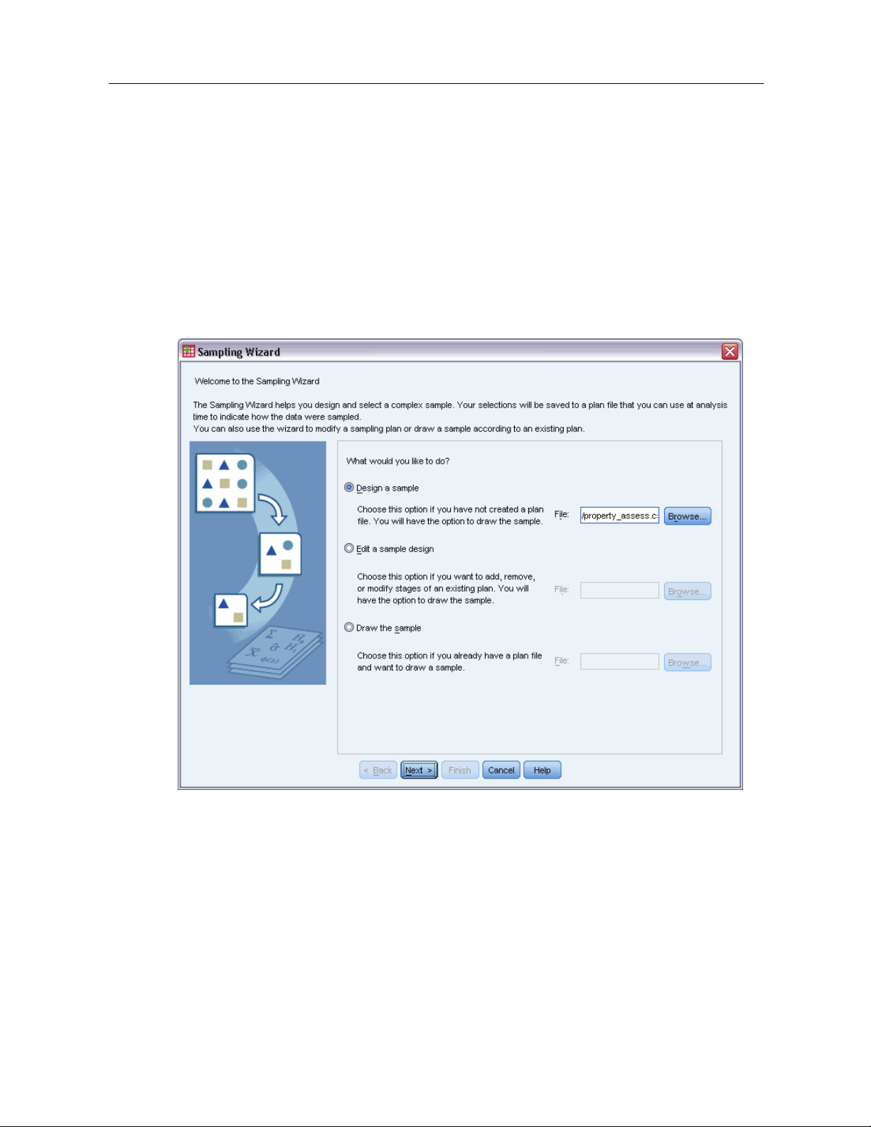
Figure 2-1

Sampling Wizard, Welcome step

Chapter

The Sampling Wizard guides you through the steps for creating, modifying, or executing a sampling plan ﬁle. Before using the Wizard, you should have a well-deﬁned target population, a list of sampling units, and an appropriate sample design in mind.

Creating a New Sample Plan

E From the menus choose:

Analyze > Complex Samples > Select a Sample...

Select Design a sample and choose a plan ﬁlename to save the sample plan.

Sampling from a Complex Design

Click Next to continue through the Wizard.

E Optionally, in the Design Variables step, you can deﬁne strata, clusters, and input sample weights.

After you deﬁne these, click

E Optionally, in the Sampling Method step, you can choose a method for selecting items.

Next.

If you select

PPS Brewer or PPS Murthy, you can click Finish to draw the sample. Otherwise,

click Next and then:

E In the Sample Size step, specify the number or proportion of units to sample.

E You can now click Finish to draw the sample.

Optionally, in further steps you can:

 Choose output variables to save.

 Add a second or third stage to the design.

 Set various selection options, including which stages to draw samples from, the random

number seed, and whether to treat user-missing values as valid values of design variables.

 Choose where to save output data.

 Paste your selections as command syntax.

Chapter 2

Sampling Wizard: Design Variables

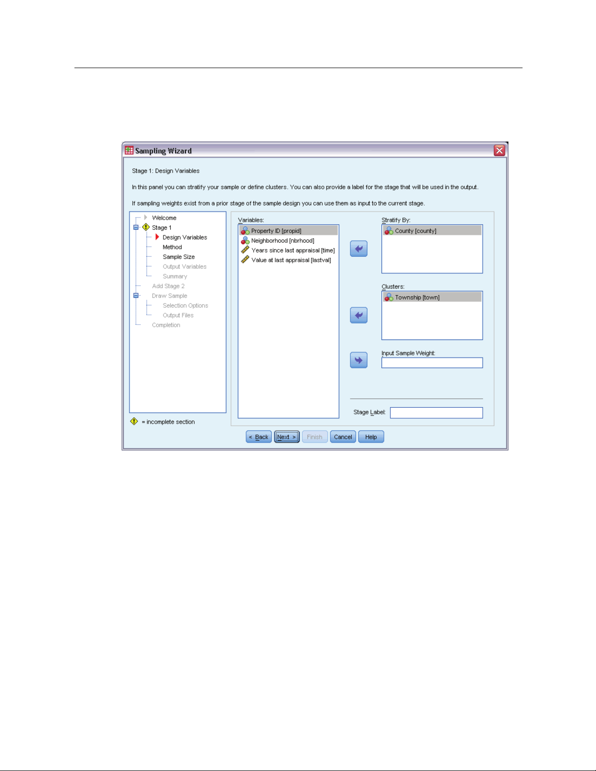
Figure 2-2

Sampling Wizard, Design Variables step

This step allows you to select stratiﬁcation and clustering variables and to deﬁne input sample weights. You can also specify a label for the stage.

Stratify By. The cross-classiﬁcation of stratiﬁcation variables deﬁnes distinct subpopulations, or

strata. Separate samples are obtained for each stratum. To improve the precision of your estimates, units within strata should be as homogeneous as possible for the characteristics of interest.

Clusters. Cluster variables deﬁne groups of observational units, or clusters. Clusters are useful

when directly sampling observational units from the population is expensive or impossible; instead, you can sample clusters from the population and then sample observational units from the selected clusters. However, the use of clusters can introduce correlations among sampling units, resulting in a loss of precision. To minimize this effect, units within clusters should be as heterogeneous as possible for the characteristics of interest. You must deﬁne at least one cluster variable in order to plan a multistage design. Clusters are also n ecessary in the use of several different sampling methods. For more information, see the topic Sampling Wizard: Sampling

Method on p. 8.

Input Sample Weight. If the current sample design is part of a larger sample design, you may have

sample weights from a previous stage of the larger design. You can specify a n umeric variable containing these weights in the ﬁrst stage of the current design. Sample weights are computed automatically for subsequent stages of the current design.

Stage Label. Youcanspecifyanoptionalstringlabelforeachstage. Thisisusedintheoutputto

help identify stagewise information.

Note: The source variable list has the same content across steps of the Wizard. In other words, variables removed from the source list in a particular step are removed from the list in all steps. Variables returned to t he source list appear in the list in all steps.

Tree Controls for Navigating the Sam pling Wizard

On the left side of each step in the Sampling Wizard is an outline of all the steps. You can navigate theWizardbyclickingonthenameofanenabled step in the outline. Steps are enabled as long as all previous steps are valid—that is, if each previous step has been given the minimum required speciﬁcations for that step. See the Help for individual steps for more information on whyagivenstepmaybeinvalid.

Sampling from a Complex Design

Chapter 2

Sampling Wizard: Sampling Method

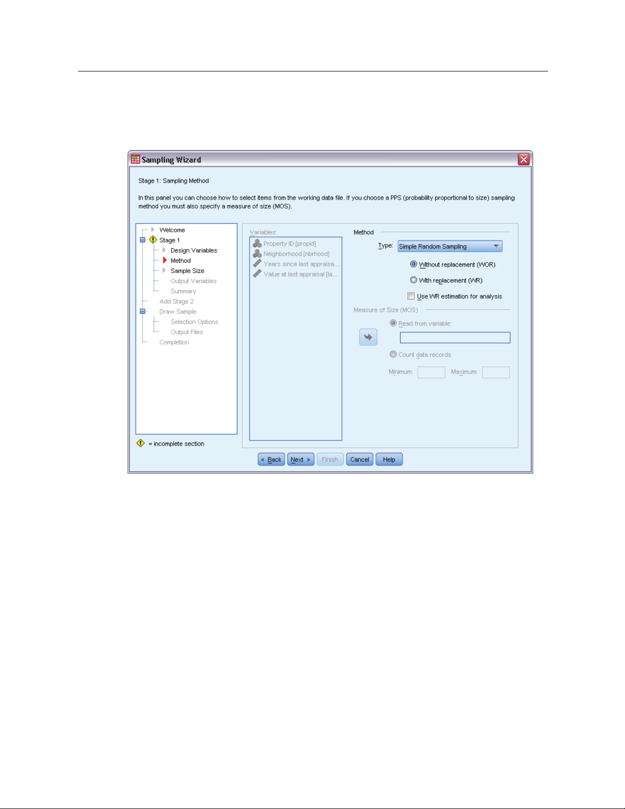
Figure 2-3

Sampling Wizard, Sampling Method step

This step allows you to specify how to select cases from the active dataset.

Method. Controls in this group are used to choose a selection method. Some sampling types allow

you to choose whether to sample with replacement (WR) or w ithout replacement (WOR). See the type descriptions for more information. Note that some probability-proportional-to-size (PPS) types are available only when clusters have been deﬁned and that all PPS types are available only in the ﬁrst stage of a design. Moreover, WR methods are available only in the last stage of a design.

 Simple Random Sampling. Units are selected with equal probability. They can be selected

with or without replacement.

 Simple Systematic. Units are selected at a ﬁxed interval throughout the sampling frame (or

strata, if they have been speciﬁed) and extracted without replacement. A randomly selected unit within the ﬁrst interval is chosen as the starting point.

 Simple Sequential. Units are selected sequentially with equal probability and without

replacement.

 PPS. This is a ﬁrst-stage method that selects units at random with probability proportional

to size. Any units can be selected with replacement; only clusters can be sampled without replacement.

Sampling from a Complex Design



PPS Systematic. This is a ﬁrst-stage method that systematically selects units with probability

proportional to size. They are selected without replacement.

 PPS Sequential. This is a ﬁrst-stage method that sequentially selects units with probability

proportional to cluster size and without replacement.

 PPS Brewer. This is a ﬁrst-stage method that selects two clusters from each stratum with

probability proportional to cluster size and without replacement. A cluster variable must be speciﬁed to use this method.

 PPS Murthy. This is a ﬁrst-stage method that selects two clusters from each stratum with

probability proportional to cluster size and without replacement. A cluster variable must be speciﬁed to use this method.

 PPS Sampford. This is a ﬁrst-stage method that selects more than two clusters from each

stratum with probability proportional to cluster size and without replacement. It is an extension of Brewer’s method. A cluster variable must be speciﬁed to use this method.

 Use WR estimation f or analysis. By default, an estimation method is speciﬁed in the plan ﬁle

that is consistent with the selected sampling method. This allows you to use with-replacement estimation even if the sampling method implies WOR estimation. This option is available only in stage 1.

Measure of Size (MOS). If a PPS method is selected, you must specify a measure of size that deﬁnes

the size of each unit. These sizes can be explicitly deﬁned in a variable or they can be computed from the data. Optionally, you can set lower and upper bounds on the MOS, overriding any values found in the MOS variable or computed from the data. These options are available only in stage 1.

Chapter 2

Sampling Wizard: Sample Size

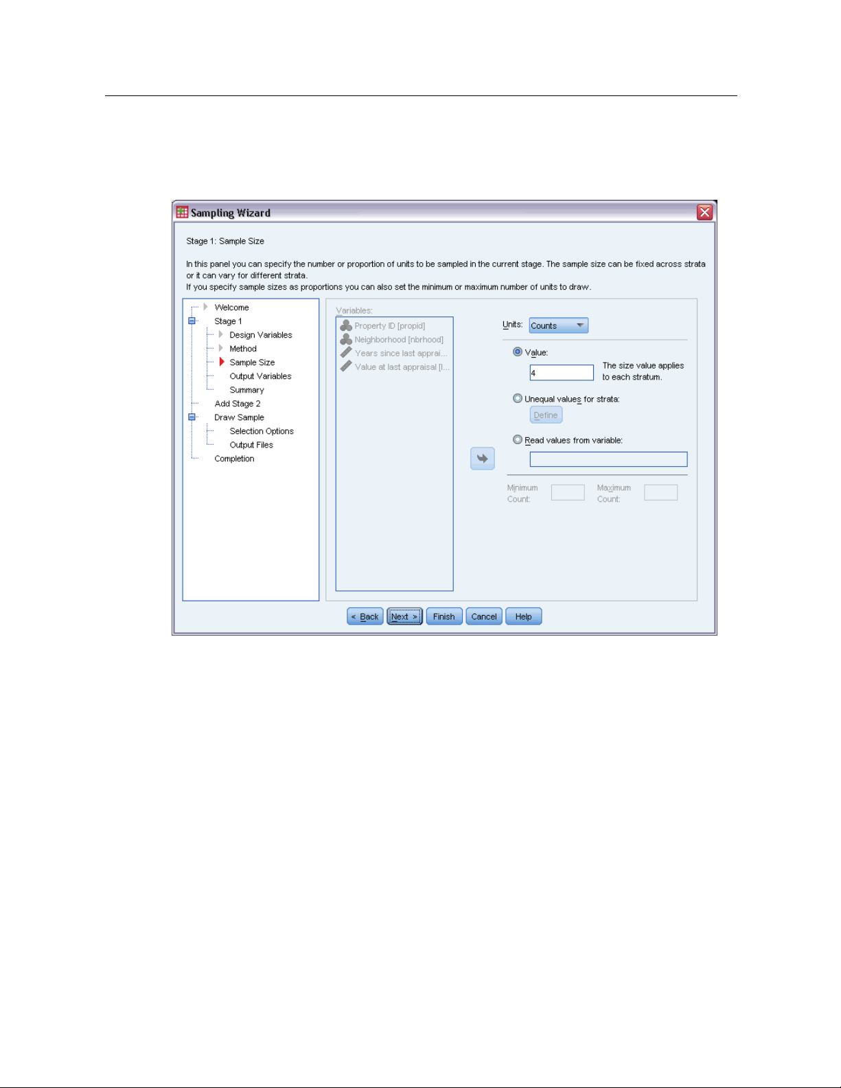
Figure 2-4

Sampling Wizard, Sample Size step

This step allows you to specify the number or proportion of units to sample within the current stage. The sample size can be ﬁxed or it can vary across strata. For the purpose of specifying sample size, clusters chosen in previous stages can be used to deﬁne strata.

Units. You can specify an exact sample size or a proportion of units to sample.

 Value. A single value is applied to all strata. If Counts is selected as the unit metric, you should

enter a positive integer. If

Proportions is selected, you should enter a non-negative value.

Unless sampling with replacement, proportion values should also be no greater than 1.

 Unequal values for strata. Allows you to enter size values on a per-stratum basis via the Deﬁne

Unequal Sizes dialog box.

 Read values from variable. Allows you to select a numeric variable that contains size values

for strata.

If Proportions is selected, you have the option to set lower and upper bounds on the number of units sampled.

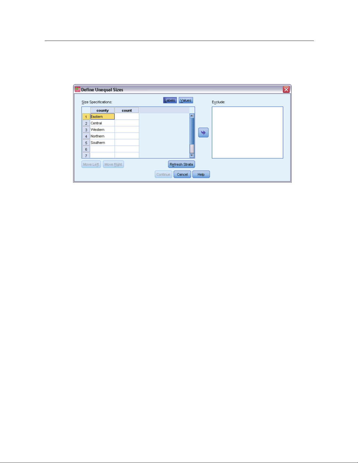
Define Unequal Sizes

Figure 2-5

Define Unequal Sizes dialog box

Sampling from a Complex Design

The Deﬁne U

Size Specifications grid. The grid displays the cross-classiﬁcations of up to ﬁve strata or

nequal Sizes dialog box allows you to enter sizes on a per-stratum basis.

cluster variables—one stratum/cluster combination per row. Eligible grid variables include all stratiﬁca

tion variables from the current and previous stages and all cluster variables from previous stages. Variables can be reordered within the grid or moved to the Exclude list. Enter sizes in the rightmost column. Click stratiﬁc

ation and cluster variables in the grid cells. Cells that contain unlabeled values always

show values. Click

Labels or Va lues to toggle the display of value labels and data values for

Refresh Strata to repopulate the grid with each combination of labeled data

values for variables in the grid.

Exclude.

To specify sizes for a subset of stratum/cluster combinations, move one or more variables

to the Exclude list. These variables are not used to deﬁne sample sizes.

Chapter 2

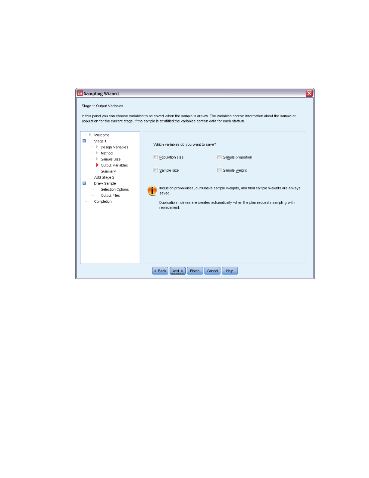
Sampling Wizard: Output Variables

Figure 2-6

Sampling Wizard, Output Variables step

This step allows you to choose variables to save when the sample is drawn.

Population size. The estimated number of units in the population for a given stage. The rootname

for the saved variable is PopulationSize_.

Sample proportion. The sampling rate at a given stage. The rootname for the saved variable is

SamplingRate_.

Sample size. The number of units drawn at a given stage. The rootname for the saved variable

is SampleSize_.

Sample weight. The inverse of the inclusion probabilities. The rootname for the saved variable is

SampleWeight_.

Some stagewise variables are generated automatically. These include:

Inclusion probabilities. The proportion of units drawn at a given stage. The rootname for the saved

variable is InclusionProbability_.

Cumulative weight. The cumulative sample weight over stages previous to and including the

current one. The rootname for the saved variable is SampleWeightCumulative_.

Index. Identiﬁes units selected multiple times within a given stage. The rootname for the saved

variable is Index_.

Note: Saved variable rootnames include an integer sufﬁxthatreﬂects the stage number—for example, PopulationSize_1_ for the saved population size for stage 1.

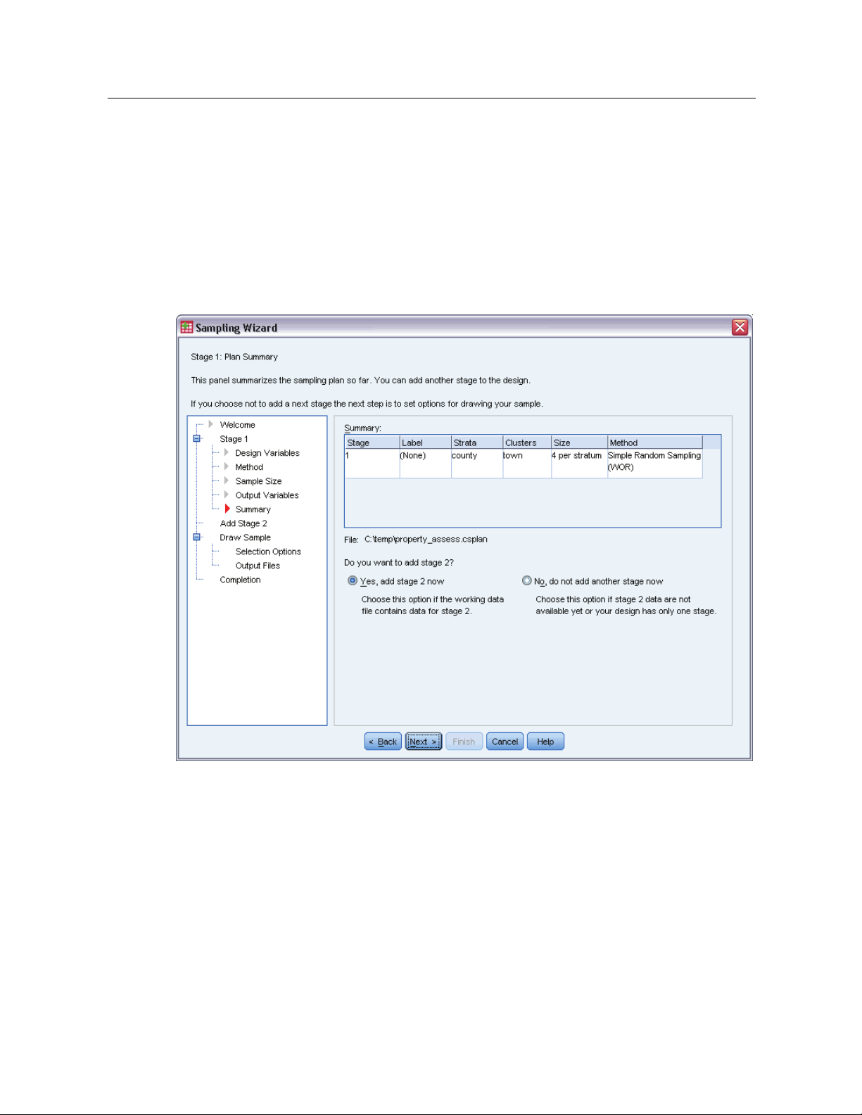
Sampling Wizard: Plan Summary

Figure 2-7

Sampling Wizard, Plan Summary step

Sampling from a Complex Design

This is the last step within each stage, providing a summary of the sample design speciﬁcations through the current stage. From here, you can either proceed to the next stage (creating it, if necessary) or set options for drawing the sample.

Chapter 2

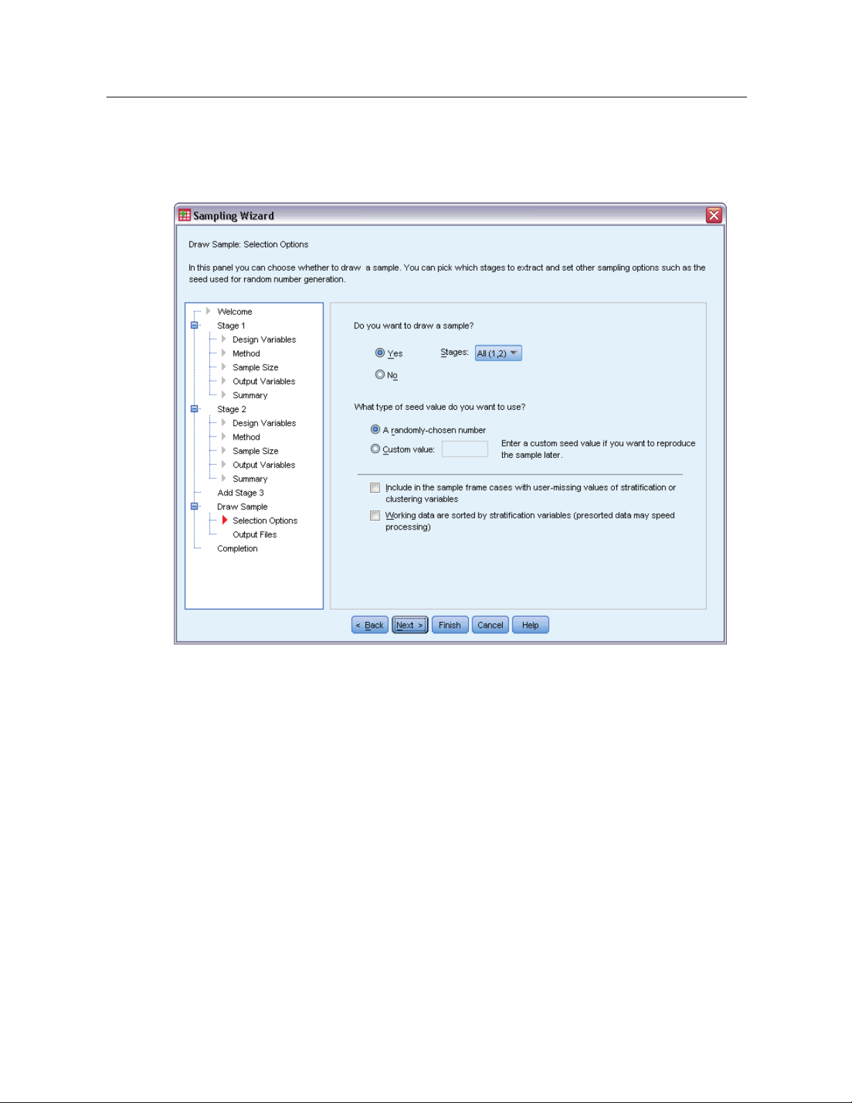
Sampling Wizard: Draw Sample Selection Options

Figure 2-8

Sampling Wizard, Draw Sample Selection Options step

This step allows you to choose whether to draw a sample. You can also control other sampling options, such as the random seed and missing-value handling.

Draw sample. In addition to choosing whether to draw a sample, you can also choose to execute

part of the sampling design. Stages must be drawn in order—that is, stage 2 cannot be drawn unless stage 1 is also drawn. When editing or executing a plan, you cannot resample locked stages.

Seed. This allows you to choose a seed value for random number generation.

Include user-missing values. This determines whether user-missing values are valid. If so,

user-missing values are treated as a separate category.

Data already sorted. If your sample frame is presorted by the values of the stratiﬁcation variables,

this option allows you to speed the selection process.

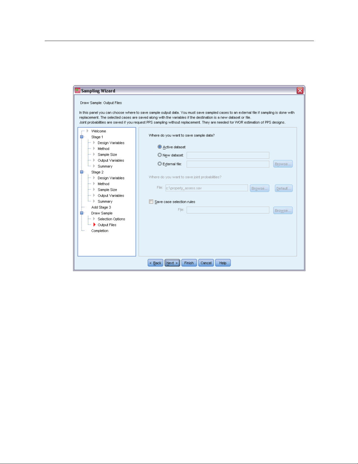
Sampling Wizard: Draw Sample Output Files

Figure 2-9

Sampling Wizard, Draw Sample Output Files step

Sampling from a Complex Design

This step allows you to choose where to direct sampled cases, weight variables, joint probabilities, and case selection rules.

Sample data. These options let you determine where sample output is written. It can be added to

the active dataset, written to a new dataset, or saved to an external IBM® SPSS® Statistics data ﬁle. Datasets are available during the current session but are not available in subsequent sessions unless you explicitly save them as data ﬁles. Dataset names must adhere to variable naming rules. If an external ﬁle or new dataset is speciﬁed, the sampling output variables and variables in the active dataset for the selected cases are written.

Joint probabilities. These options let you determine where joint probabilities are written. They are

saved to an external SPSS Statistics data ﬁle. Joint probabilities are produced if the PPS WOR, PPS Brewer, PPS Sampford, or PPS Murthy method is selected and WR estimation is not speciﬁed.

Case selection rules. If you are constructing your sample one stage at a time, you may want to

save the case selection rules to a text ﬁle. They are useful for constructing the subframe for subsequent stages.

Chapter 2

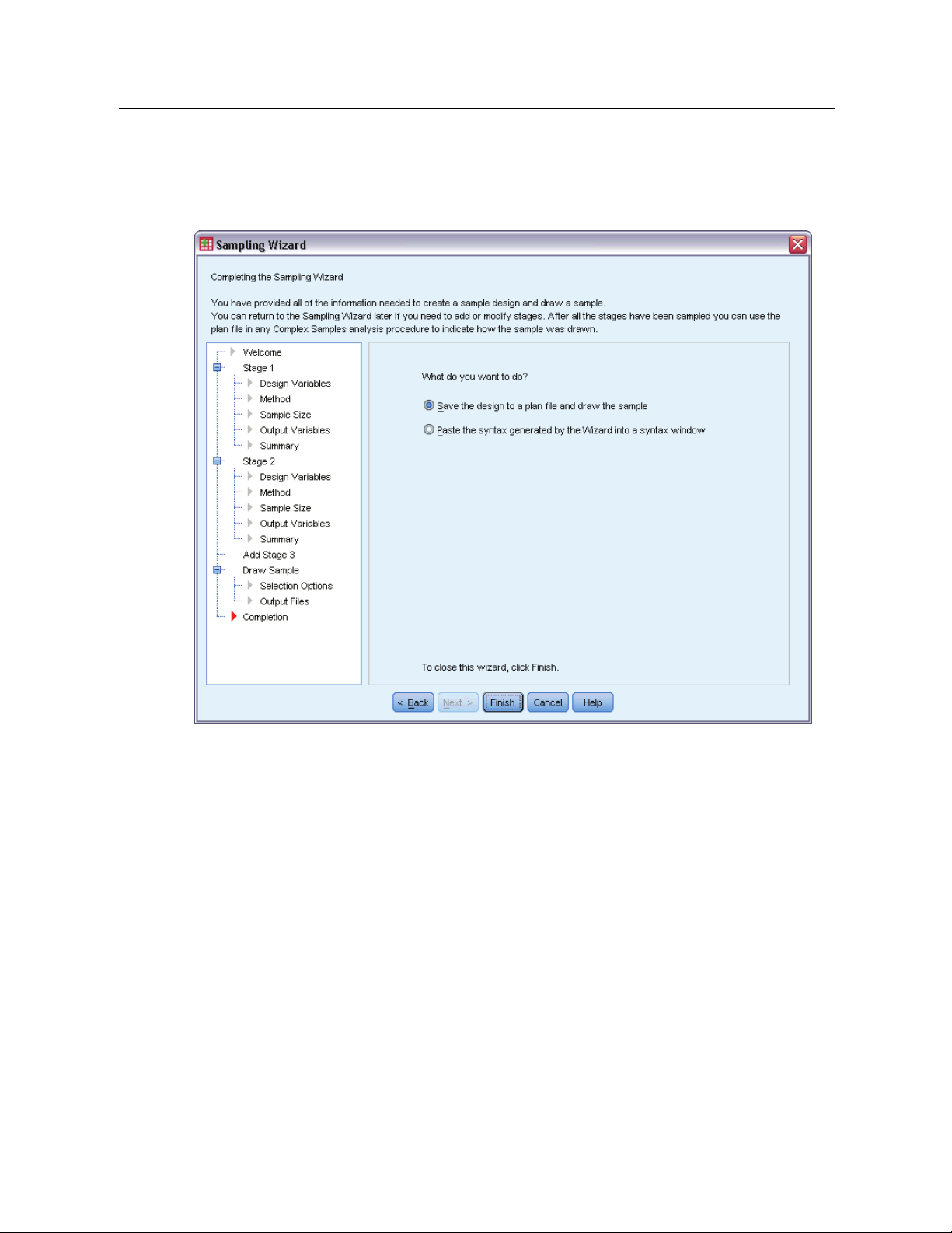
Sampling Wizard: Finish

Figure 2-10

Sampling Wizard, Finish step

This is the ﬁnal step. You can save the plan ﬁle and draw the sample now or paste your selections into a syntax window.

When making changes to stages in the existing plan ﬁle, you can save the edited plan to a new ﬁle or overwrite the existing ﬁle. When adding stages without making changes to existing stages, the Wizard automatically overwrites the existing plan ﬁle. If you want to save the plan to a new ﬁle, select

Paste the syntax generated by the Wizard into a syntax window and change the

ﬁlename in the syntax commands.

Modifying an Existing Sample Plan

E From the menus choose:

Analyze > Complex Samples > Select a Sample...

Select Editasampledesignand choose a plan ﬁle to edit.

E Click Next to continue through the Wizard.

ReviewthesamplingplaninthePlanSummarystep,andthenclickNext.

Subsequent steps are largely the same as for a new design. See the Help for individual steps for more information.

E Navigate to the Finish step, and specify a new name for the edited plan ﬁle or choose to overwrite

the existing plan ﬁle.

Optionally, you can:

 Specify stages that have already been sampled.

 Remove stages from the plan.

Sampling Wizard: Plan Summary

Figure 2-11

Sampling Wizard, Plan Summary step

Sampling from a Complex Design

This step allows you to review the sampling plan and indicate stages that have already been sampled. If editing a plan, you can also remove stages from the plan.

Previously sampled stages. If an extended sampling frame is not available, you will have to execute

a multistage sampling design one stage at a time. Select which stages have already been sampled from the drop-down list. Any stages that have been executed are locked; they are not available in the Draw Sample Selection Options step, and they cannot be altered when editing a plan.

Chapter 2

Remove stages. You can remove stages 2 and 3 from a multistage design.

Running an Existing Sample Plan

E From the menus choose:

Analyze > Complex Samples > Select a Sample...

Select Draw a sample and choose a plan ﬁle to run.

E Click Next to continue through the Wizard.

E ReviewthesamplingplaninthePlanSummarystep,andthenclickNext.

E The individual steps containing stage information are skipped when executing a sample plan. You

can now go on to the Finish step at any time.

Optionally, you can specify stages that have already been sampled.

CSPLAN and CSSELECT Commands Additional Features

The command syntax language also allows you to:

 Specify custom names for output variables.

 Control the output in the Viewer. For example, you can suppress the stagewise summary of

the plan that is displayed if a sample is designed or modiﬁed, suppress the summary of the distribution of sampled cases by strata that is shown if the sample design is executed, and request a case processing summary.

 Choose a subset of variables in the active dataset to write to an external sample ﬁle or to

a different dataset.

See the Command Syntax Reference for complete syntax information.

Preparing a Complex Sample for Analysis

Figure 3-1

Analysis Preparation Wizard, Welcome step

Chapter

The Analysis Preparation Wizard guides you through the steps for creating or modifying an analysis plan for use with the various Complex Samples analysis procedures. Before using the

rd, you should have a sample drawn according to a complex design.

Wiza

Creating a new plan is most useful when you do not have access to the samp ling plan ﬁle used to draw the sample (recall that the sampling plan contains a default analysis plan). If you do

access to the sampling plan ﬁle used to draw the sample, you can use the default analysis

have plan contained in the sampling plan ﬁle or override the default analysis speciﬁcations and save your changes to a new ﬁle.

Chapter 3

Creating a New Analysis Plan

E From the menus choose:

Analyze > Complex

Select Createaplanfile,andchooseaplanﬁlename to which you will save the analysis plan.

Samples > Prepare for Analysis...

E Click Next to continue t

E Specify the variable containing sample weights in the Design Variables step, optionally deﬁning

hrough the Wizard.

strata and clusters.

E You can now click Finish to save the plan.

Optionally, in further steps you can:

 Select the method for estimating standard errors in the Estimation Method step.

 Specify the number of units sampled or the inclusion probability per unit in the Size step.

 Add a second or third stage to the design.

 Paste your selections as command syntax.

Analysis Preparation Wizard: Design Variables

Figure 3-2

Analysis Preparation Wizard, Design Variables step

Preparing a Compl ex Sample for Analysis

This step allows you to identify t he stratiﬁcation and clustering variables and deﬁne sample weights. You can also provide a label for the stage.

Strata. The cross-classiﬁcation of stratiﬁcation variables deﬁnes distinct subpopulations, or strata.

Your total sample represents the combination of independent samples from each stratum.

Clusters. Cluster variables deﬁne groups of observational units, or clusters. Samples drawn in

multiple stages select clusters in the earlier stages and then subsample units from the s elected clusters. When analyzing a data ﬁle obtained by sampling clusters with replacement, you should include the duplication index as a cluster variable.

Sample Weight. You must provide sample weights in the ﬁrst stage. Sample weights are computed

automatically for subsequent stages of the current design.

Stage Label. Youcanspecifyanoptionalstringlabelforeachstage. Thisisusedintheoutputto

help identify stagewise information.

Note: The source variable list has the same contents across steps of the Wizard. In other words, variables removed from the source list in a particular step are removed from the list in all steps. Variables returned to the source list show up in all steps.

Tree Controls for Navigating the Analysis Wizard

At the left side of each step of the Analysis Wizard is an outline of all the steps. You can navigate the Wizard by clicking on the name of an enabled step in the outline. Steps are enabled as long as all previous steps are valid—that is, as long as each previous step has b een given the minimum required speciﬁcations for that step. For more information on why a given step may be invalid, see the Help for individual steps.

Chapter 3

Analysis Preparation Wizard: Estimation Method

Figure 3-3

Analysis Preparation Wizard, Estimation Method step

This step allows you to spec

WR (sampling with replacement). WR estimation does not include a correction for sampling from a

ify an estimation method for the stage.

ﬁnite population (FPC) when estimating the variance under the complex sampling design. You can choose to include or exclude the FPC when estimating the variance under simple random sampling (SRS).

Choosing not to include the FPC for SRS variance estimation is recommended when the analysis weights have been scaled so that they do not add up to the population size. The SRS variance estimate is used in computing statistics like the design effect. WR estimation can be speciﬁed only in the ﬁnal stage of a design; the Wizard will not allow you to add another stage if you select WR estimation.

Equal WOR (equal probability sampling without replacement). Equal WOR estimation includes the

ﬁnite population correction and assumes that units are sampled with equal probability. Equal WOR can be speciﬁed in any stage of a design.

Unequal WOR (unequal probability sampling without replacement). In addition to using the ﬁnite

population correction, Unequal WOR accounts for sampling units (usually clusters) selected with unequal probability. This estimation method is available only in the ﬁrst stage.

Analysis Preparation Wizard: Size

Figure 3-4

Analysis Preparation Wizard, Size step

Preparing a Compl ex Sample for Analysis

This step is used to specify inclusion probabilities or population sizes for the current stage. Sizes can be ﬁxed or can vary across strata. For the purpose of specifying sizes, clusters speciﬁed in

us stages can be used to deﬁne strata. Note that this step is necessary only when Equal

previo WOR is chosen as the Estimation Method.

Units. You can specify exact population sizes or the probabilities with which units were sampled.

 Value. A single value is applied to all strata. If Population Sizes is selected as the unit metric,

you should enter a non-negative integer. If avalue

 Unequ

between 0 and 1, inclusive.

al values for strata.

Allows you to enter size values on a per-stratum basis via the Deﬁne

Inclusion Probabilities is selected, you should enter

Unequal Sizes dialog box.

 Read values from variable. Allows you to select a numeric variable that contains size values

for strata.

Chapter 3

Define Unequal Sizes

Figure 3-5

Define Unequal Sizes dialog box

The Deﬁne U

Size Specifications grid. The grid displays the cross-classiﬁcations of up to ﬁve strata or

nequal Sizes dialog box allows you to enter sizes on a per-stratum basis.

cluster variables—one stratum/cluster combination per row. Eligible grid variables include all stratiﬁca

ation and cluster variables in the grid cells. Cells that contain unlabeled values always

show values. Click

Labels or Va lues to toggle the display of value labels and data values for

Refresh Strata to repopulate the grid with each combination of labeled data

values for variables in the grid.

Exclude.

To specify sizes for a subset of stratum/cluster combinations, move one or more variables

to the Exclude list. These variables are not used to deﬁne sample sizes.

Analysis Preparation Wizard: Plan Summary

Figure 3-6

Analysis Preparation Wizard, Plan Summary step

Preparing a Compl ex Sample for Analysis

This is the last step within each stage, providing a summary of the analysis design speciﬁcations through the current stage. From here, you can either proceed to the next stage (creating it if

ary) or save the analysis speciﬁcations.

necess

If you cannot add another stage, it is likely because:

 No cluster variable was speciﬁed in the Design Variables step.

 You selected WR estimation in the Estimation Method step.

 This is the third stage of the analysis, and the Wizard supports a maximum of three stages.

Chapter 3

Analysis Preparation Wizard: Finish

Figure 3-7

Analysis Preparation Wizard, Finish step

This is t

he ﬁnal step. You can save the plan ﬁle now or paste your selections to a syntax window.

When making changes to stages in the existing plan ﬁle,youcansavetheeditedplantoanew ﬁle or overwrite the existing ﬁle. When adding stages without making changes to existing stages, the Wiza new ﬁle, choose to

rd automatically overwrites the existing plan ﬁle. If you want to save the plan to a

Paste the syntax generated by the Wizard into a syntax window and change the

ﬁlename in the syntax commands.

Modifying an Existing Analysis Plan

E From the menus choose:

Analyze > Complex Samples > Prep are for Analysis...

Select Edit a plan file, and choose a plan ﬁlename to which you will save the analysis plan.

E Click Next to continue through the Wizard.

Review the analysis plan in the Plan Summary step, and then click Next.

Subsequent steps are largely the same as for a new design. For more information, see the Help for individual steps.

E Navigate to the Finish step, and specify a new name for the edited plan ﬁle, or choose to overwrite

the existing plan ﬁle.

Optionally, you can remove stages from the plan.

Analysis Preparation Wizard: Plan Summary

Figure 3-8

Analysis Preparation Wizard, Plan Summary step

Preparing a Compl ex Sample for Analysis

This step allows you to review the analysis plan and remove stages from the plan.

Remove Stages. You can remove stages 2 and 3 from a multistage design. Since a plan must have

at least one stage, you can edit but not remove stage 1 from the design.

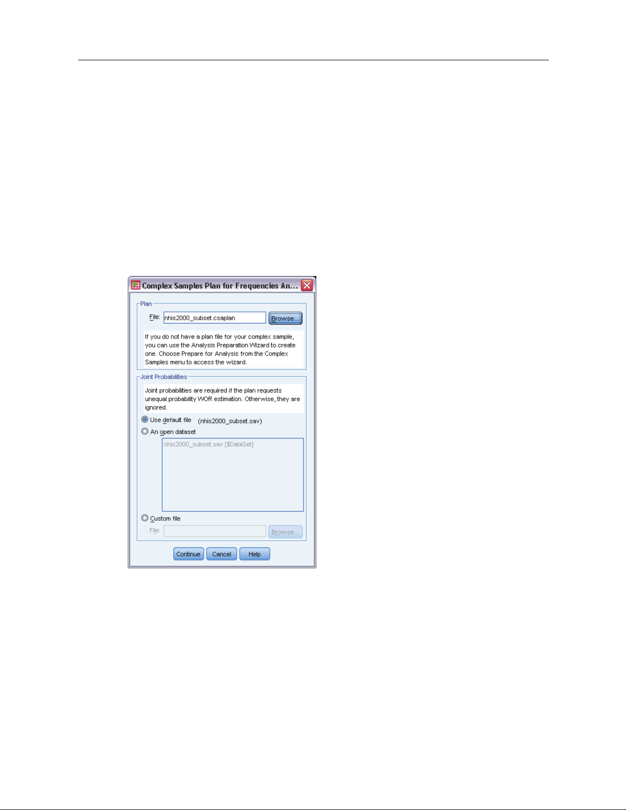
Complex Samples Plan

Complex Samples analysis procedures require analysis speciﬁcations from an analysis or sample plan ﬁle in order to provide valid results.

Figure 4-1

Complex Samples Plan dialog box

Chapter

Plan. Specify the path of an analysis or sample plan ﬁle.

Joint Probabilities. In order to use Unequal WOR estimation for clusters drawn using a PPS WOR

method, you need to specify a separate ﬁle or an open dataset containing the joint probabilities. This ﬁle or dataset is created by the Sampling Wizard during sampling.

Complex Samples Frequencies

The Complex Samples Frequencies procedure produces frequency tables for selected variables and displays univariate statistics. Optionally, you can request statistics by subgroups, deﬁned by one or more categorical variables.

Example. Using the Complex Samples Frequencies procedure, you can obtain univariate tabular

statistics for vitamin usage among U.S. citizens, based on the results of the National Health Interview Survey (NHIS) and with an appropriate analysis plan for this public-use data.

Statistics. The procedure produces estimates of cell population sizes and table percentages,

plus standard errors, conﬁdence intervals, coefﬁcients of variation, design effects, square roots of design effects, cumulative values, and unweighted counts for each estimate. Additionally, chi-square and likelihood-ratio statistics are computed for the test of equal cell proportions.

Chapter

Data. Variables for which frequency tables are produced should be categorical. Subpopulation

variables can be string or numeric but should be categorical.

Assumptions. The cases in the data ﬁle represent a sample from a complex design that should

be analyzed according to the speciﬁcations in the ﬁle selected in the Complex Samples Plan

dialog box.

Obtaining Complex Samples Freq uen cies

E From the menus choose:

Analyze > Complex Samples > Frequencies...

Select a plan ﬁle. Optionally, select a custom joint probabilities ﬁle.

E Click Continue.

Chapter 5

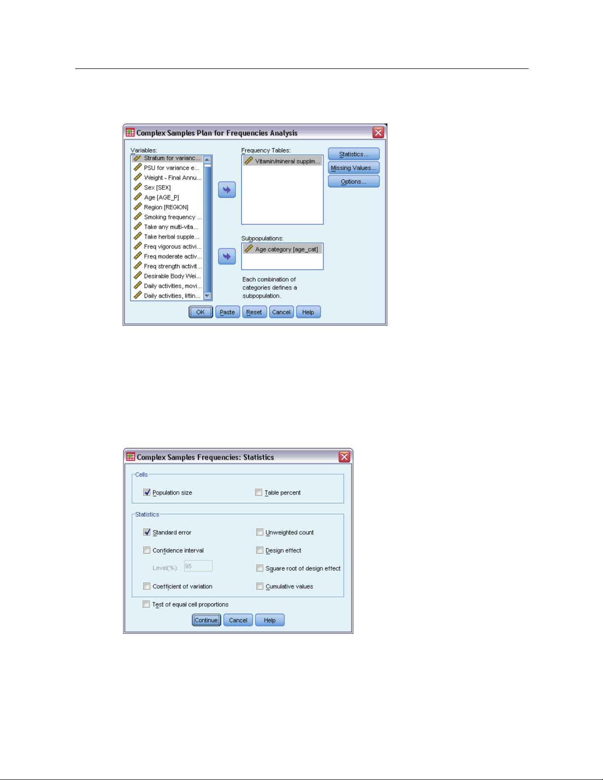
Figure 5-1

Frequencies dialog box

E Select at least one frequency variable.

Optionally, you can specify variables to deﬁne subpopulations. Statistics are computed separately for each subpopulation.

Complex Samples Frequencies Statistics

Figure 5-2

Frequencies Statistics dial og box

Cells. This group allows you to request estimates of the cell population sizes and table percentages.

Statistics. This group produces statistics associated with the population size or table percentage.

 Standard error. The standard error of the estimate.



Confidence interval. Aconﬁdence interval for the estimate, using the speciﬁed level.

 Coefficient of variation. The ratio of the standard error of the estimate to the estimate.

 Unweighted count. The number of units used to compute the estimate.

 Design effect. The ratio of the variance of the estimate to the variance obtained by assuming

that the sample is a simple random sample. This is a measure of the effect of specifying a complex design, where values further from 1 indicate greater effects.

 Square root of design effect. This is a measure of the effect of specifying a complex design,

where values further from 1 indicate greater effects.

 Cumulative values. The cumulative estimate through each value of the variable.

Test of equal cell proportions. This produces chi-square and likelihood-ratio tests of the hypothesis

that the categories of a variable have equal fre quencies. Separate tests are performed for each variable.

Complex Samples Missing Values

Figure 5-3

Missing Values dialog box

Complex Samples Frequencies

Tables. This group determines which cases are used in the analysis.

 Use all available data. Missing values are determined on a table-by-table basis. Thus, the cases

used to compute statistics may vary across frequency or crosstabulation tables.

 Use consistent case base. Missing values are determined across all variables. Thus, the cases

used to compute statistics are consistent across tables.

Categorical Design Variables. This group determines whether user-missing values are valid

or invalid.

Chapter 5

Complex Samples Options

Figure 5-4

Options dialog box

Subpopulation Display. You can choose to have subpopulations displayed in the same table or in

separate tables.

Complex Samples Descriptives

The Complex Samples Descriptives procedure displays univariate summary statistics for several variables. Optionally, you can request statistics by subgroups, deﬁned by one or more categorical variables.

Example. Using the Complex Samples Descriptives procedure, you can obtain univariate

descriptive statistics for the activity levels of U.S. citizens, based on the results of the National Health Interview Survey (NHIS) and with an appropriate analysis plan for this public-use data.

Statistics. The procedure produces means and sums, plus t tests, standard errors, conﬁdence

intervals, coefﬁcients of variation, unweighted counts, population sizes, design effects, and square roots of design effects for each estimate.

Data. Measures should be scale variables. Subpopulation variables can be string or numeric

but should be categorical.

Chapter

Assumptions. The cases in the data ﬁle represent a sample from a complex design that should

be analyzed according to the speciﬁcations in the ﬁle selected in the Complex Samples Plan

dialog box.

Obtaining Complex Samples Descriptives

E From the menus choose:

Analyze > Complex Samples > Descriptives...

Select a plan ﬁle. Optionally, select a custom joint probabilities ﬁle.

E Click Continue.

Chapter 6

Figure 6-1

Descriptives dialog box

E Select at least one measure variable.

Optionally, you can specify variables to deﬁne subpopulations. Statistics are computed separately for each subpopulation.

Complex Samples Descriptives Statistics

Figure 6-2

Descriptives Statistics dialog box

Summaries. This group allows you to request estimates of the means and sums of the measure

variables. Additionally, you can request t tests of the estimates against a speciﬁed value.

Statistics. This group produces statistics associated with the mean or sum.

 Standard error. The standard error of the estimate.

 Confidence interval. Aconﬁdence interval for the estimate, using the speciﬁed level.

 Coefficient of variation. The ratio of the standard error of the estimate to the estimate.

 Unweighted count. The number of units used to compute the estimate.

 Population size. The estimated number of units in the population.

 Design effect. The ratio of the variance of the estimate to the variance obtained by assuming

that the sample is a simple random sample. This is a measure of the effect of specifying a complex design, where values further from 1 indicate greater effects.

 Square root of design effect. This is a measure of the effect of specifying a complex design,

where values further from 1 indicate greater effects.

Complex Samples Descriptives Missing Values

Figure 6-3

Descriptives Missing Values dialog box

Complex Samples Descriptives

Statistics for Measure Variables. This group determines which cases are used in the analysis.

 Use all available data. Missing values are determined on a variable-by-variable basis, thus the

cases used to compute statistics may vary across measure variables.

 Ensure consistent case base. Missing values are determined across all variables, thus the

cases used to compute statistics are consistent.

Categorical Design Variables. This group determines whether user-missing values are valid

or invalid.

Chapter 6

Complex Samples Options

Figure 6-4

Options dialog box

Subpopulation Display. You can choose to have subpopulations displayed in the same table or in

separate tables.

Complex Samples Crosstabs

The Complex Samples Crosstabs procedure produces crosstabulation tables for pairs of selected variables and displays two-way statistics. Optionally, you can request statistics by subgroups, deﬁned by one or more categorical variables.

Example. Using the Complex Samples Crosstabs procedure, you can obtain cross-classiﬁcation

statistics for smoking frequency by vitamin usage of U.S. citizens, based on the results of the National Health Interview Survey (NHIS) and with an appropriate analysis plan for this public-use data.

Statistics. The procedure produces estimates of cell population sizes and row, column, and table

percentages, plus standard errors, conﬁdence intervals, coefﬁcients of variation, expected values, design effects, square roots of design effects, residuals, adjusted residuals, and unweighted counts for each estimate. The odds ratio, relative risk, and risk difference are computed for 2-by-2 tables. Additionally, Pearson and likelihood-ratio statistics are computed for the test of independence of the row and column variables.

Chapter

Data. Row and column variables should be categorical. Subpopulation variables can be string or

numeric but should be categorical.

Assumptions. The cases in the data ﬁle represent a sample from a complex design that should

be analyzed according to the speciﬁcations in the ﬁle selected in the Complex Samples Plan

dialog box.

Obtaining Complex Samples Crosstabs

E From the menus choose:

Analyze > Complex Samples > Crosstabs...

Select a plan ﬁle. Optionally, select a custom joint probabilities ﬁle.

E Click Continue.

Chapter 7

Figure 7-1

Crosstabs dialog box

E Select at least one row variable and one column variable.

Optionally, you can specify variables to deﬁne subpopulations. Statistics are computed separately for each subpopulation.

Complex Samples Crosstabs Statistics

Figure 7-2

Crosstabs Statistics dialog box

Complex Samples Crosstabs

Cells. This group allows you to request estimates of the cell population size and row, column,

and table percentages.

Statistics. This group produces statistics associated with the population size and row, column,

and table percentages.

 Standard error. The standard error of the estimate.

 Confidence interval. Aconﬁdence interval for the estimate, using the speciﬁed level.

 Coefficient of variation. The ratio of the standard error of the estimate to the estimate.

 Expected values. The expected value of the estimate, under the hypothesis of independence

of the row and column variable.

 Unweighted count. The number of units used to compute the estimate.

 Design effect. The ratio of the variance of the estimate to the variance obtained by assuming

that the sample is a simple random sample. This is a measure of the effect of specifying a complex design, where values further from 1 indicate greater effects.

 Square root of design effect. This is a measure of the effect of specifying a complex design,

where values further from 1 indicate greater effects.

 Residuals. The expected value is the number of cases that you would expect in the cell if there

were no relationship between the two variables. A positive residual indicates that there are more cases in the cell than there would be if the row and column variables were independent.

 Adjusted residuals. The residual for a cell (observed minus expected value) divided by an

estimate of its standard error. The resulting standardized residual is expressed in standard deviation units above or below the mean.

Chapter 7

Summaries for 2-by-2 Tables. This group produces statistics for tables in which the row and column

variable each have two categories. Each is a measure of the strength of the association between the presence of a factor and the occurrence of an event.

 Odds ratio. The odds ratio can be u sed as an estimate of relative risk when the occurrence

of the factor is rare.

 Relative risk. The ratio of the risk of an event in the presence of the factor to the risk of the

event in the absence of the factor.

 Risk difference. The difference between the risk of an event in the presence of the factor and

the risk of the event in the absence of the factor.

Test of independence of rows and columns. This produces chi-square and likelihood-ratio tests of

the hypothesis that a row and column variable are independent. Separate tests are performed for each pair of variables.

Complex Samples Missing Values

Figure 7-3

Missing Values dialog box

Tables. This group determines which cases are used in the analysis.

 Use all available data. Missing values are determined on a table-by-table basis. Thus, the cases

used to compute statistics may vary across frequency or crosstabulation tables.

 Use consistent case base. Missing values are determined across all variables. Thus, the cases

used to compute statistics are consistent across tables.

Categorical Design Variables. This group determines whether user-missing values are valid

or invalid.

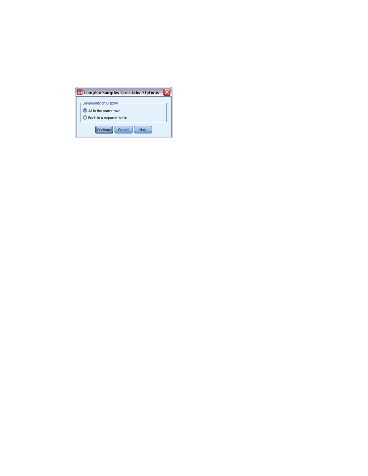
Complex Samples Options

Figure 7-4

Options dialog box

Subpopulation Display. You can choose to have subpopulations displayed in the same table or in

separate tables.

Complex Samples Crosstabs

Complex Samples Ratios

The Complex Samples Ratios procedure displays univariate summary statistics for ratios of variables. Optionally, you can request statistics by subgroups, deﬁned by one or more categorical variables.

Example. Using the Complex Samples Ratios procedure, you can obtain descriptive statistics for

the ratio of current property value to last assessed value, based on the results of a statewide survey carried out according to a complex design and with an appropriate analysis plan for the data.

Statistics. The procedure produces ratio estimates, t tests, standard errors, conﬁdence intervals,

coefﬁcients of variation, unweighted counts, population sizes, design effects, and square roots of design effects.

Data. Numerators and denominators should be positive-valued scale variables. Subpopulation

variables can be string or numeric but should be categorical.

Chapter

Assumptions. The cases in the data ﬁle represent a sample from a complex design that should

be analyzed according to the speciﬁcations in the ﬁle selected in the Complex Samples Plan

dialog box.

Obtaining Complex Samples Ratios

E From the menus choose:

Analyze > Complex Samples > Ratios...

Select a plan ﬁle. Optionally, select a custom joint probabilities ﬁle.

E Click Continue.

Figure 8-1

Ratios dialog box

E Select at least one numerator variable and denominator variable.

Complex Samples Ratios

Optionally, you can specify variables to deﬁne subgroups for which statistics are produced.

Complex Samples Ratios Statistics

Figure 8-2

Ratios Statistics dialog box

Statistics. This group produces statistics associated with the ratio estimate.

 Standard error. The standard error of the estimate.

 Confidence interval. Aconﬁdence interval for the estimate, using the speciﬁed level.

 Coefficient of variation. The ratio of the standard error of the estimate to the estimate.

 Unweighted count. The number of units used to compute the estimate.

 Population size. The estimated number of units in the population.

Chapter 8



Design effect. The ratio of the variance of the estimate to the variance obtained by assuming

that the sample is a simple random sample. This is a measure of the effect of specifying a complex design, where values further from 1 indicate greater effects.

 Square root of design effect. This is a measure of the effect of specifying a complex design,

where values further from 1 indicate greater effects.

Ttest. You can request t tests of the estimates against a speciﬁ

Complex Samples Ratios Missing Values

Figure 8-3

Ratios Missing Values dialog box

Ratios. This group determines which cases are used in the analysis.

 Use all available data. Missing values are determined on a ratio-by-ratio basis. Thus, the cases

used to compute statistics may vary across numerator-denominator pairs.

 Ensure consistent case base. Missing values are determined across all variables. Thus, the

cases used to compute statistics are consistent.

ed value.

Categorical Design Variables. This group determines whether user-missing values are valid

or invalid.

Complex Samples Options

Figure 8-4

Options dialog box

Subpopulation Display. You can choose to have subpopulations displayed in the same table or in

separate tables.

Complex Samples General Linear Model

The Complex Samples General Linear Model (CSGLM) procedure performs linear regression analysis, as well as analysis of variance and covariance, for samples drawn by complex sampling methods. Optionally, you can request analyses for a subpopulation.

Example. A grocery store chain surveyed a set of customers concerning their purchasing habits,

according to a complex design. Given the survey results and how much e ach customer spent in the previous month, the store wants to see if the frequency with which customers shop is related to the amount they spend in a month, controlling for the gender of the customer and incorporating the sampling design.

Chapter

Statistics. The procedure produces estimates, standard errors, conﬁdence intervals, t tests, design

effects, and square roots of design effects for model parameters, as well as the correlations and covariances between parameter estimates. Measures of model ﬁt and descriptive statistics for the dependent and independent variables are also available. Additionally, you can request estimated marginal means for levels of model factors and factor interactions.

Data. The dependent variable is quantitative. Factors are categorical. Covariates are quantitative

variables that are related to the dependent variable. Subpopulation variables can b e string or numeric but should be categorical.

Assumptions. The cases in the data ﬁle represent a sample from a complex design that should

be analyzed according to the speciﬁcations in the ﬁle selected in the Complex Samples Plan

dialog box.

Obtaining a Complex Samples General Linear M odel

From the menus choose:

Analyze > Complex Samples > General Linear Model...

Select a plan ﬁle. Optionally, select a custom joint probabilities ﬁle.

E Click Continue.

Chapter 9

Figure 9-1

General Linear Model dialog box

E Select a dependent variable.

Optionally, you can:

 Select variables for factors and covariates, as appropriate for your data.

 Specify a variable to deﬁne a subpopulation. The analysis is performed only for the selected

category of the subpopulation variable.

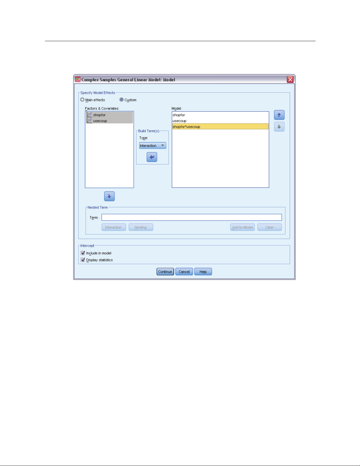
Figure 9-2

Model dialog box

Complex Samples Ge neral Linear Model

Specify Model Effects. By default, the procedure builds a main-effects model using the factors

and covariates speciﬁed in the main dialog box. Alternatively, you can build a custom model that includes interaction effects and nested terms.

Non-Nested Terms

For the selected factors and covariates:

Interaction. Creates the highest-level interaction term for all selected variables.

Main effects. Creates a main-effects term for each variable selected.

All 2-way. Creates all possible two-way interactions of the selected variables.

All 3-way. Creates all possible three-way interactions of the selected variables.

All 4-way. Creates all possible four-way interactions of the selected variables.

All 5-way. Creates all possible ﬁve-way interactions of the selected variables.

Chapter 9

Nested Terms

n may follow the spending habits of its customers a t several store locations. Since each customer frequents only one of these locations, the Customer effect can be said to be nested within the Store location effect.

Additionally, you can include in

teraction effects, such as polynomial terms involving the same

covariate, or add multiple levels of nesting to the nested term.

Limitations. Nested terms have the following restrictions:

 All factors within an interaction must be unique. Thus, if A is a factor, then specifying A*A

is invalid.

 All factors within a nested effect must be unique. Thus, if A is a factor, then specifying A(A)

is invalid.

 No effect can be nested within a covariate. Thus, if A is a factor and X is a covariate, then

specifying A(X) is invalid.

Intercept. The intercept is usually included in the model. If you can assume the data pass through

the origin, you can exclude the intercept. Even if you include the intercept in the model, you can choose to suppress statistics related to it.

Complex Samples General Linear Model Statistics

Figure 9-3

General Linear Model Statistics dialog box

Model Parameters. This group allows you to control the display of statistics related to the model

parameters.

 Estimate. Displays estimates of the coefﬁcients.

 Standard error. Displays the standard error for each coefﬁcient estimate

 Confidence interval. Displays a conﬁdence interval for each coefﬁcient e

conﬁdence level for the interval is set in the Options dialog box.

 Ttest. Displays a t test of each coefﬁcient estimate. The null hypothesis for each test is that

thevalueofthecoefﬁcient is 0.

stimate. The

Complex Samples Ge neral Linear Model



Covariances of parameter estimates. Displays an estimate of the covariance matrix for the

model coefﬁcients.

 Correlations of parameter estimates. Displays an estimate of the correlation matrix for the

model coefﬁcients.

 Design effect. The ratio of the variance of the estimate to the variance obtained by assuming

that the sample is a simple random sample. This is a measure of the effect of specifying a complex design, where values further from 1 indicate greater effects.

 Square root of design effect. This is a measure of the effect of specifying a complex design,

where values further from 1 indicate greater effects.

Model fit. Displays R

Population means of dependent variable and covariates. Displays summary information about the

and root mean squared error statistics.

dependent variable, covariates, and factors.

Sample design information. Displays summary information about the sample, including the

unweighted count and the population size.

Complex Samples Hypothesis Tests

Figure 9-4

Hypothesis Tests dialog box

Test Statistic. This group allows you to select the type of statistic used for testing hypotheses. You

can choose between F,adjustedF, chi-square, and adjusted chi-square.

Sampling Degrees of Freedom. This group gives you control over the sampling design degrees of

freedomusedtocomputep values for all test statistics. If based on the sampling design, the value is the difference between the number of primary sampling units and the number of strata in the

Chapter 9

ﬁrst stage of sampling. Alternatively, you can set a custom degrees of freedom by specifying a positive integer.

Adjustment for Multiple Comparisons. When performing hypothesis tests with multiple contrasts,

the overall signiﬁcance level can be adjusted from the signiﬁcance levels for the included contrasts. This group allows you to choose the adjustment method.

 Least significant difference. This method does not control the overall probability of rejecting

the hypotheses that some linear contrasts are different from the null hypothesis values.

 Sequential Sidak. This is a sequentially step-down rejective Sidak procedure that is much

less conservative in terms of rejecting individual hypotheses but maintains the same overall signiﬁcance level.

 Sequential Bonferroni. This is a sequentially step-down rejective Bonferroni procedure that is

much less conservative in terms of rejecting individual hypotheses but maintains the same overall signiﬁcance level.

 Sidak. This method provides tighter bounds than the Bonferroni approach.

 Bonferroni. This method adjusts the observed signiﬁcance level for the fact that multiple

contrasts are being tested.

Complex Samples General Linear Model Estimated Means

Figure 9-5

General Linear Model Estimated Means dialog box

Complex Samples Ge neral Linear Model

The Estimated Means dialog box allows you to display the model-estimated marginal means for levels of factors and factor interactions speciﬁed in the Model subdialog box. You can also request that the overall population mean be displayed.

Term. Estimated means are computed for the selected factors and factor interactions.

Contrast. The contrast determines how hypothesis tests are set up to compare the estimated means.

 Simple. Compares the mean of each level to the mean of a speciﬁed level. This type of contrast

is useful when there is a control group.

 Deviation. Compares the mean of each level (except a reference category) to the mean of all of

the levels (grand mean). The levels of the factor can be in any order.

 Difference. Compares the mean of each level (except the ﬁrst) to the mean of previous levels.

They are sometimes called reverse Helmert contrasts.

 Helmert. Compares the mean of each level of the factor (except the last) to the mean of

subsequent levels.

 Repeated. Compares the mean of each level (except the last) to the mean of the subsequent

level.

 Polynomial. Compares the linear effect, quadratic effect, cubic effect, and so on. The

ﬁrst degree of freedom contains the linear effect across all categories; the second degree of freedom, the quadratic effect; and so on. These contrasts are often used to estimate polynomial trends.

Reference Category. The simple and deviation contrasts require a reference category or factor

level against which the others are compared.

Complex Samples General Linear Model Save

Figure 9-6

General Linear Model Save dialog box

Save Variables. This group allows you to save the model predicted values and residuals as new

variables in the working ﬁle.

Chapter 9

Export model as SPSS Statistics data. Writes a dataset in IBM® SPSS® Statistics format containing

the parameter correlation or covariance matrix with parameter estimates, standard errors, signiﬁcance values, and degrees of freedom. The order of variables in the matrix ﬁ le is as follows.

 rowtype_. Takes values (and value labels), COV (Covariances), CORR (Correlations), EST

(Parameter estimates), SE (Standard errors), SIG (Signiﬁcance levels), and DF (Sampling design degrees of freedom). There is a separate case with row type COV (or CORR) for each model parameter, plus a separate case for each of the other row types.

 varname_. Takes values P1, P2, ..., corresponding to an ordered list of all model parameters,

for row types COV or CORR, with value labels corresponding to the parameter strings shown in the parameter estimates table. The cells are blank for other row types.

 P1, P2, ... These variables correspond to an ordered list of all model parameters, with variable

labels corresponding to the parameter strings shown in the parameter estimates table, and take values according to the row type. For redundant parameters, all covariances are set to zero; correlations are set to the system-missing value; all parameter estimates are set at zero; and all standard errors, signiﬁcance levels, and residual degrees of freedom are set to the system-missing value.

Note:Thisﬁle is not immediately usable for further analyses in other procedures that read a matrix ﬁle unless those procedures accept all the row types exported here.

Export Model as XML. Saves the parameter estimates and the parameter covariance matrix, if

selected, in XML (PMML) format. You can use this model ﬁle to apply the model information to other data ﬁles for scoring purposes.

Complex Samples General Linear Model Options

Figure 9-7

General Linear Model Options dialog box

User-Missing Values. All design variables, as well as the dependent variable and any covariates,

must have valid data. Cases with invalid data for any of these variables are deleted from the analysis. These controls allow you to decide whether user-missing values are treated as valid among the strata, cluster, subpopulation, and factor variables.

Confidence Interval. This is the conﬁdence interval level for coefﬁcient estimates and estimated

marginal means. Specify a value greater than or equal to 50 and less than 100.

CSGLM Command Additional Features

The command syntax language also allows you to:

 Specify custom tests of effects versus a linear combination of effects or a value (using the

CUSTOM subcommand).

 Fix covariates at values other than their means when computing estimated marginal means

(using the

 Specify a metric for polynomial contrasts (using the EMMEANS subcommand).

 Specify a tolerance value for checking singularity (using the CRITERIA subcommand).

 Create user-speciﬁed names for saved variables (using the SAVE subcommand).

 Produce a general estimable function table (using the PRINT subcommand).

See the Command Syntax Reference for complete syntax information.

EMMEANS subcommand).

Complex Samples Ge neral Linear Model

Chapter

Complex Samples Logistic Regression

The Complex Samples Logistic Regression procedure performs logistic regression analysis on a binary or multinomial dependent variable for samples drawn by complex sampling methods. Optionally, you can request analyses for a subpopulation.

Example. Aloanofﬁcer has collected past records of customers given loans at several different

branches, according to a complex design. While incorporating the sample design, the ofﬁcer wants to see if the probability with which a customer defaults is related to age, employment history, and amount of credit debt.

Statistics. The procedure produces estimates, exponentiated estimates, standard errors, conﬁdence

intervals, t tests, design effects, and square roots of design effects for model parameters, as well as

the correlations and covariances between parameter estimates. Pseudo R tables, and descriptive statistics for the dependent and independent variables are also available.

statistics, classiﬁcation

Data. The dependent variable is categorical. Factors are categorical. Covariates are quantitative

variables that are related to the dependent variable. Subpopulation variables can b e string or numeric but should be categorical.

Assumptions. The cases in the data ﬁle represent a sample from a complex design that should

be analyzed according to the speciﬁcations in the ﬁle selected in the Complex Samples Plan

dialog box.

Obtaining Complex Samples Logistic Regression

From the menus choose:

Analyze > Complex Samples > Logistic Regression...

Select a plan ﬁle. Optionally, select a custom joint probabilities ﬁle.

E Click Continue.

Figure 10-1

Logistic Regression dialog box

Complex Samples Logistic Regression

E Select a dependent variable.

Optionally, you can:

 Select variables for factors and covariates, as appropriate for your data.

 Specify a variable to deﬁne a subpopulation. The analysis is performed only for the selected

category of the subpopulation variable.

Complex Samples Logistic Regression Reference Category

Figure 10-2

Logistic Regression Reference Category dialog box

Chapter 10

By default, the Complex Samples Logistic Regression procedure makes the highest-valued category the reference category. This dialog box allows you to specify the highest value, the lowest value, or a custom category as the reference category.

Complex Samples Logistic Regression Model

Figure 10-3

Logistic Regression Model dialog box

Specify Model Effects. By default, the procedure builds a main-effects model using the factors

and covariates speciﬁed in the main dialog box. Alternatively, you can build a custom model that includes interaction effects and nested terms.

Non-Nested Terms

For the selected factors and covariates:

Interaction. Creates the highest-level interaction term for all selected variables.

Main effects. Creates a main-effects term for each variable selected.

All 2-way. Creates all possible two-way interactions of the selected variables.

Complex Samples Logistic Regression

All 3-way. Creates all possible three-way interactions of the selected variables.

All 4-way. Creates all possible four-way interactions of the selected variables.

All 5-way. Creates all possible ﬁve-way interactions of the selected variables.

Nested Terms

You can build nested terms for your model in this procedure. Nested terms are useful for modeling the effect of a factor or covariate whose values do not interact with the levels of anoth

er factor. For example, a grocery store chain may follow the spending habits of its customers at several store locations. Since each customer frequents only one of these locations, the Customer effect can be said to be nested within the Store location effect.

Additionally, you can include interaction effects, such as polynomial terms involving the same

covariate, or add multiple levels of nesting to the nested term.

Limitations. Nested terms have the following restrictions:

 All factors within an interaction must be unique. Thus, if A is a factor, then specifying A*A

is invalid.

 All factors within a nested effect must be unique. Thus, if A is a factor, then specifying A(A

)

is invalid.

 No effect can be nested within a covariate. Thus, if A is a factor and X is a covariate, then

specifying A(X) is invalid.

Intercept. The intercept is usually included in the model. If you can assume the data pass through

the origin, you can exclude the intercept. Even if you include the intercept in the model, you can choose to suppress statistics related to it.

Complex Samples Logistic Regression Statistics

Figure 10-4

Logistic Regression Statistics dialog box

Model Fit. Controls the display of statistics that measure the overall model performance.

Chapter 10



Pseudo R-square. The R

statistic from linear regression does not have an exact counterpart

among logistic regression models. There are, instead, multiple measures that attempt to mimic

the properties of the R

 Classification table. Displays the tabulated cross-classiﬁcations of the observed category by

statistic.

the model-predicted category on the dependent variable.

Parameters. This group allows you to control the display of statistics related to the model

parameters.

 Estimate. Displays estimates of the coefﬁcients.

 Exponentiated estimate. Displays the base of the natural logarithm raised to the power of the

estimates of the coefﬁcients. While the estimate has nice properties for statistical testing, the exponentiated estimate, or exp(B), is easier to interpret.

 Standard error. Displays the standard error for each coefﬁcient estimate.

 Confidence interval. Displays a conﬁdence interval for each coefﬁcient estimate. The

conﬁdence level for the interval is set in the Options dialog box.

 Ttest. Displays a t test of each coefﬁcient estimate. The null hypothesis for each test is that

thevalueofthecoefﬁcient is 0.

 Covariances of parameter estimates. Displays an estimate of the covariance matrix for the

model coefﬁcients.

 Correlations of parameter estimates. Displays an estimate of the correlation matrix for the

model coefﬁcients.

 Design effect. The ratio of the variance of the estimate to the variance obtained by assuming

that the sample is a simple random sample. This is a measure of the effect of specifying a complex design, where values further from 1 indicate greater effects.

 Square root of design effect. This is a measure of the effect of specifying a complex design,

where values further from 1 indicate greater effects.

Summary statistics for model variables. Displays summary information about the dependent

variable, covariates, and factors.

Sample design information. Displays summary information about the sample, including the

unweighted count and the population size.

Complex Samples Hypothesis Tests

Figure 10-5

Hypothesis Tests dialog box

Complex Samples Logistic Regression

Test Statistic. This group allows you to select the type of statistic used for testing hypotheses. You

can choose between F,adjustedF, chi-square, and adjusted chi-square.

Sampling Degrees of Freedom. This group gives you control over the sampling design degrees of

freedomusedtocomputep values for all test statistics. If based on the sampling design, the value is the difference between the number of primary sampling units and the number of strata in the ﬁrst stage of sampling. Alternatively, you can set a custom degrees of freedom by specifying a positive integer.