IBM SPSS Amos 21 User Manual

IBM® SPSS® Amos™ 21 User’s Guide

James L. Arbuckle

Note: Before using this information and the product it supports, read the information in the “Notices” section on page 631.

This edition applies to IBM® SPSS® Amos™ 21 and to all subsequent releases and modifications until otherwise indicated in new editions.

Microsoft product screenshots reproduced with permission from Microsoft Corporation.

Licensed Materials - Property of IBM

AMOS is a trademark of Amos Development Corporation.

Part I: Getting Started

1 Introduction 1

Featured Methods . . . . . . . . . . . . . . . . . . . . . . . . . . . . . . . . 2

About the Tutorial . . . . . . . . . . . . . . . . . . . . . . . . . . . . . . . . 3

About the Examples . . . . . . . . . . . . . . . . . . . . . . . . . . . . . . . 3

About the Documentation . . . . . . . . . . . . . . . . . . . . . . . . . . . .4

Other Sources of Information. . . . . . . . . . . . . . . . . . . . . . . . . . 4

Acknowledgements . . . . . . . . . . . . . . . . . . . . . . . . . . . . . . . 5

2 Tutorial: Getting Started with

Amos Graphics 7

Introduction . . . . . . . . . . . . . . . . . . . . . . . . . . . . . . . . . . . .7

About the Data . . . . . . . . . . . . . . . . . . . . . . . . . . . . . . . . . .8

Launching Amos Graphics . . . . . . . . . . . . . . . . . . . . . . . . . . . 9

Creating a New Model. . . . . . . . . . . . . . . . . . . . . . . . . . . . . 10

Specifying the Data File . . . . . . . . . . . . . . . . . . . . . . . . . . . . 11

Specifying the Model and Drawing Variables . . . . . . . . . . . . . . . 11

Naming the Variables . . . . . . . . . . . . . . . . . . . . . . . . . . . . . 12

Drawing Arrows . . . . . . . . . . . . . . . . . . . . . . . . . . . . . . . . 13

Constraining a Parameter . . . . . . . . . . . . . . . . . . . . . . . . . . . 14

Altering the Appearance of a Path Diagram . . . . . . . . . . . . . . . . 15

To Move an Object . . . . . . . . . . . . . . . . . . . . . . . . . . . . 15

To Reshape an Object or Double-Headed Arrow . . . . . . . . . . . 15

To Delete an Object. . . . . . . . . . . . . . . . . . . . . . . . . . . . 15

To Undo an Action . . . . . . . . . . . . . . . . . . . . . . . . . . . . 16

To Redo an Action . . . . . . . . . . . . . . . . . . . . . . . . . . . . 16

iii

Setting Up Optional Output . . . . . . . . . . . . . . . . . . . . . . . . . . 16

Performing the Analysis . . . . . . . . . . . . . . . . . . . . . . . . . . . . 18

Viewing Output . . . . . . . . . . . . . . . . . . . . . . . . . . . . . . . . . 18

To View Text Output . . . . . . . . . . . . . . . . . . . . . . . . . . . 18

To View Graphics Output . . . . . . . . . . . . . . . . . . . . . . . . 19

Printing the Path Diagram. . . . . . . . . . . . . . . . . . . . . . . . . . . 20

Copying the Path Diagram . . . . . . . . . . . . . . . . . . . . . . . . . . 21

Copying Text Output . . . . . . . . . . . . . . . . . . . . . . . . . . . . . . 21

Part II: Examples

1 Estimating Variances and Covariances 23

Introduction . . . . . . . . . . . . . . . . . . . . . . . . . . . . . . . . . . 23

About the Data . . . . . . . . . . . . . . . . . . . . . . . . . . . . . . . . . 23

Bringing In the Data . . . . . . . . . . . . . . . . . . . . . . . . . . . . . . 24

Analyzing the Data . . . . . . . . . . . . . . . . . . . . . . . . . . . . . . . 25

Specifying the Model. . . . . . . . . . . . . . . . . . . . . . . . . . . 25

Naming the Variables . . . . . . . . . . . . . . . . . . . . . . . . . . 26

Changing the Font . . . . . . . . . . . . . . . . . . . . . . . . . . . . 27

Establishing Covariances . . . . . . . . . . . . . . . . . . . . . . . . 27

Performing the Analysis . . . . . . . . . . . . . . . . . . . . . . . . . 28

Viewing Graphics Output . . . . . . . . . . . . . . . . . . . . . . . . . . . 28

Viewing Text Output . . . . . . . . . . . . . . . . . . . . . . . . . . . . . . 29

Optional Output . . . . . . . . . . . . . . . . . . . . . . . . . . . . . . . . . 33

Calculating Standardized Estimates . . . . . . . . . . . . . . . . . . 33

Rerunning the Analysis . . . . . . . . . . . . . . . . . . . . . . . . . 34

Viewing Correlation Estimates as Text Output . . . . . . . . . . . . 34

Distribution Assumptions for Amos Models . . . . . . . . . . . . . . . . 35

Modeling in VB.NET . . . . . . . . . . . . . . . . . . . . . . . . . . . . . . 36

Generating Additional Output . . . . . . . . . . . . . . . . . . . . . . 39

Modeling in C# . . . . . . . . . . . . . . . . . . . . . . . . . . . . . . . . . 39

Other Program Development Tools . . . . . . . . . . . . . . . . . . . . . 40

2 Testing Hypotheses 41

Introduction . . . . . . . . . . . . . . . . . . . . . . . . . . . . . . . . . . .41

About the Data. . . . . . . . . . . . . . . . . . . . . . . . . . . . . . . . . .41

Parameters Constraints . . . . . . . . . . . . . . . . . . . . . . . . . . . .41

Constraining Variances . . . . . . . . . . . . . . . . . . . . . . . . . .42

Specifying Equal Parameters. . . . . . . . . . . . . . . . . . . . . . .43

Constraining Covariances . . . . . . . . . . . . . . . . . . . . . . . .44

Moving and Formatting Objects . . . . . . . . . . . . . . . . . . . . . . . .45

Data Input . . . . . . . . . . . . . . . . . . . . . . . . . . . . . . . . . . . .46

Performing the Analysis. . . . . . . . . . . . . . . . . . . . . . . . . .47

Viewing Text Output . . . . . . . . . . . . . . . . . . . . . . . . . . . .47

Optional Output . . . . . . . . . . . . . . . . . . . . . . . . . . . . . . . . .48

Covariance Matrix Estimates. . . . . . . . . . . . . . . . . . . . . . .49

Displaying Covariance and Variance Estimates

on the Path Diagram. . . . . . . . . . . . . . . . . . . . . . . . . . . .51

Labeling Output . . . . . . . . . . . . . . . . . . . . . . . . . . . . . . . . .51

Hypothesis Testing . . . . . . . . . . . . . . . . . . . . . . . . . . . . . . .52

Displaying Chi-Square Statistics on the Path Diagram . . . . . . . . . . .53

Modeling in VB.NET. . . . . . . . . . . . . . . . . . . . . . . . . . . . . . .55

Timing Is Everything . . . . . . . . . . . . . . . . . . . . . . . . . . . .57

3 More Hypothesis Testing 59

Introduction . . . . . . . . . . . . . . . . . . . . . . . . . . . . . . . . . . .59

About the Data. . . . . . . . . . . . . . . . . . . . . . . . . . . . . . . . . .59

Bringing In the Data. . . . . . . . . . . . . . . . . . . . . . . . . . . . . . .59

Testing a Hypothesis That Two Variables Are Uncorrelated . . . . . . .60

Specifying the Model . . . . . . . . . . . . . . . . . . . . . . . . . . . . . .60

Viewing Text Output . . . . . . . . . . . . . . . . . . . . . . . . . . . . . .62

Viewing Graphics Output. . . . . . . . . . . . . . . . . . . . . . . . . . . .63

Modeling in VB.NET. . . . . . . . . . . . . . . . . . . . . . . . . . . . . . .65

4 Conventional Linear Regression 67

Introduction . . . . . . . . . . . . . . . . . . . . . . . . . . . . . . . . . . . 67

About the Data . . . . . . . . . . . . . . . . . . . . . . . . . . . . . . . . . 67

Analysis of the Data . . . . . . . . . . . . . . . . . . . . . . . . . . . . . . 68

Specifying the Model . . . . . . . . . . . . . . . . . . . . . . . . . . . . . 69

Identification . . . . . . . . . . . . . . . . . . . . . . . . . . . . . . . . . . 70

Fixing Regression Weights . . . . . . . . . . . . . . . . . . . . . . . . . . 70

Viewing the Text Output . . . . . . . . . . . . . . . . . . . . . . . . . . . . 72

Viewing Graphics Output . . . . . . . . . . . . . . . . . . . . . . . . . . . 74

Viewing Additional Text Output. . . . . . . . . . . . . . . . . . . . . . . . 75

Modeling in VB.NET . . . . . . . . . . . . . . . . . . . . . . . . . . . . . . 77

Assumptions about Correlations among Exogenous Variables . . . 77

Equation Format for the AStructure Method . . . . . . . . . . . . . 78

5 Unobserved Variables 81

Introduction . . . . . . . . . . . . . . . . . . . . . . . . . . . . . . . . . . . 81

About the Data . . . . . . . . . . . . . . . . . . . . . . . . . . . . . . . . . 81

Model A . . . . . . . . . . . . . . . . . . . . . . . . . . . . . . . . . . . . . 83

Measurement Model . . . . . . . . . . . . . . . . . . . . . . . . . . . . . 83

Structural Model . . . . . . . . . . . . . . . . . . . . . . . . . . . . . . . . 84

Identification . . . . . . . . . . . . . . . . . . . . . . . . . . . . . . . . . . 85

Specifying the Model . . . . . . . . . . . . . . . . . . . . . . . . . . . . . 85

Changing the Orientation of the Drawing Area . . . . . . . . . . . . 86

Creating the Path Diagram . . . . . . . . . . . . . . . . . . . . . . . 87

Rotating Indicators . . . . . . . . . . . . . . . . . . . . . . . . . . . . 88

Duplicating Measurement Models. . . . . . . . . . . . . . . . . . . 88

Entering Variable Names . . . . . . . . . . . . . . . . . . . . . . . . 90

Completing the Structural Model . . . . . . . . . . . . . . . . . . . . 90

Results for Model A . . . . . . . . . . . . . . . . . . . . . . . . . . . . . . 90

Viewing the Graphics Output . . . . . . . . . . . . . . . . . . . . . . 93

Model B . . . . . . . . . . . . . . . . . . . . . . . . . . . . . . . . . . . . .93

Results for Model B . . . . . . . . . . . . . . . . . . . . . . . . . . . . . . .94

Testing Model B against Model A. . . . . . . . . . . . . . . . . . . . . . .96

Modeling in VB.NET. . . . . . . . . . . . . . . . . . . . . . . . . . . . . . .98

Model A . . . . . . . . . . . . . . . . . . . . . . . . . . . . . . . . . . .98

Model B . . . . . . . . . . . . . . . . . . . . . . . . . . . . . . . . . . .99

6 Exploratory Analysis 101

Introduction . . . . . . . . . . . . . . . . . . . . . . . . . . . . . . . . . . 101

About the Data. . . . . . . . . . . . . . . . . . . . . . . . . . . . . . . . . 101

Model A for the Wheaton Data . . . . . . . . . . . . . . . . . . . . . . . 102

Specifying the Model . . . . . . . . . . . . . . . . . . . . . . . . . . 102

Identification . . . . . . . . . . . . . . . . . . . . . . . . . . . . . . . 103

Results of the Analysis . . . . . . . . . . . . . . . . . . . . . . . . . 103

Dealing with Rejection . . . . . . . . . . . . . . . . . . . . . . . . . 104

Modification Indices. . . . . . . . . . . . . . . . . . . . . . . . . . . 105

Model B for the Wheaton Data . . . . . . . . . . . . . . . . . . . . . . . 107

Text Output . . . . . . . . . . . . . . . . . . . . . . . . . . . . . . . . 108

Graphics Output for Model B . . . . . . . . . . . . . . . . . . . . . . 109

Misuse of Modification Indices . . . . . . . . . . . . . . . . . . . . 110

Improving a Model by Adding New Constraints . . . . . . . . . . . 110

Model C for the Wheaton Data . . . . . . . . . . . . . . . . . . . . . . . 114

Results for Model C . . . . . . . . . . . . . . . . . . . . . . . . . . . 114

Testing Model C . . . . . . . . . . . . . . . . . . . . . . . . . . . . . 115

Parameter Estimates for Model C . . . . . . . . . . . . . . . . . . . 115

Multiple Models in a Single Analysis . . . . . . . . . . . . . . . . . . . . 116

Output from Multiple Models . . . . . . . . . . . . . . . . . . . . . . . . 119

Viewing Graphics Output for Individual Models . . . . . . . . . . . 119

Viewing Fit Statistics for All Four Models. . . . . . . . . . . . . . . 119

Obtaining Optional Output . . . . . . . . . . . . . . . . . . . . . . . 121

Obtaining Tables of Indirect, Direct, and Total Effects . . . . . . . 122

vii

Modeling in VB.NET . . . . . . . . . . . . . . . . . . . . . . . . . . . . . 123

Model A . . . . . . . . . . . . . . . . . . . . . . . . . . . . . . . . . 123

Model B . . . . . . . . . . . . . . . . . . . . . . . . . . . . . . . . . 124

Model C . . . . . . . . . . . . . . . . . . . . . . . . . . . . . . . . . 125

Fitting Multiple Models. . . . . . . . . . . . . . . . . . . . . . . . . 126

7 A Nonrecursive Model 129

Introduction . . . . . . . . . . . . . . . . . . . . . . . . . . . . . . . . . . 129

About the Data . . . . . . . . . . . . . . . . . . . . . . . . . . . . . . . . 129

Felson and Bohrnstedt’s Model . . . . . . . . . . . . . . . . . . . . . . 130

Model Identification . . . . . . . . . . . . . . . . . . . . . . . . . . . . . 131

Results of the Analysis . . . . . . . . . . . . . . . . . . . . . . . . . . . 131

Text Output . . . . . . . . . . . . . . . . . . . . . . . . . . . . . . . 131

Obtaining Standardized Estimates . . . . . . . . . . . . . . . . . . 133

Obtaining Squared Multiple Correlations . . . . . . . . . . . . . . 133

Graphics Output. . . . . . . . . . . . . . . . . . . . . . . . . . . . . 134

Stability Index . . . . . . . . . . . . . . . . . . . . . . . . . . . . . . 135

Modeling in VB.NET . . . . . . . . . . . . . . . . . . . . . . . . . . . . . 136

8 Factor Analysis 137

Introduction . . . . . . . . . . . . . . . . . . . . . . . . . . . . . . . . . . 137

About the Data . . . . . . . . . . . . . . . . . . . . . . . . . . . . . . . . 137

A Common Factor Model . . . . . . . . . . . . . . . . . . . . . . . . . . 138

Identification . . . . . . . . . . . . . . . . . . . . . . . . . . . . . . . . . 139

Specifying the Model . . . . . . . . . . . . . . . . . . . . . . . . . . . . 140

Drawing the Model . . . . . . . . . . . . . . . . . . . . . . . . . . . 140

Results of the Analysis . . . . . . . . . . . . . . . . . . . . . . . . . . . 141

Obtaining Standardized Estimates . . . . . . . . . . . . . . . . . . 142

Viewing Standardized Estimates . . . . . . . . . . . . . . . . . . . 143

Modeling in VB.NET . . . . . . . . . . . . . . . . . . . . . . . . . . . . . 144

viii

9 An Alternative to Analysis of Covariance 145

Introduction . . . . . . . . . . . . . . . . . . . . . . . . . . . . . . . . . . 145

Analysis of Covariance and Its Alternative . . . . . . . . . . . . . . . . 145

About the Data. . . . . . . . . . . . . . . . . . . . . . . . . . . . . . . . . 146

Analysis of Covariance . . . . . . . . . . . . . . . . . . . . . . . . . . . . 147

Model A for the Olsson Data. . . . . . . . . . . . . . . . . . . . . . . . . 147

Identification. . . . . . . . . . . . . . . . . . . . . . . . . . . . . . . . . . 148

Specifying Model A . . . . . . . . . . . . . . . . . . . . . . . . . . . . . . 149

Results for Model A . . . . . . . . . . . . . . . . . . . . . . . . . . . . . . 149

Searching for a Better Model . . . . . . . . . . . . . . . . . . . . . . . . 149

Requesting Modification Indices . . . . . . . . . . . . . . . . . . . 149

Model B for the Olsson Data. . . . . . . . . . . . . . . . . . . . . . . . . 150

Results for Model B . . . . . . . . . . . . . . . . . . . . . . . . . . . . . . 151

Model C for the Olsson Data . . . . . . . . . . . . . . . . . . . . . . . . . 153

Drawing a Path Diagram for Model C . . . . . . . . . . . . . . . . . 154

Results for Model C . . . . . . . . . . . . . . . . . . . . . . . . . . . . . . 154

Fitting All Models At Once . . . . . . . . . . . . . . . . . . . . . . . . . . 154

Modeling in VB.NET. . . . . . . . . . . . . . . . . . . . . . . . . . . . . . 155

Model A . . . . . . . . . . . . . . . . . . . . . . . . . . . . . . . . . . 155

Model B . . . . . . . . . . . . . . . . . . . . . . . . . . . . . . . . . . 155

Model C . . . . . . . . . . . . . . . . . . . . . . . . . . . . . . . . . . 156

Fitting Multiple Models . . . . . . . . . . . . . . . . . . . . . . . . . 157

10 Simultaneous Analysis of Several Groups 159

Introduction . . . . . . . . . . . . . . . . . . . . . . . . . . . . . . . . . . 159

Analysis of Several Groups . . . . . . . . . . . . . . . . . . . . . . . . . 159

About the Data. . . . . . . . . . . . . . . . . . . . . . . . . . . . . . . . . 160

Model A . . . . . . . . . . . . . . . . . . . . . . . . . . . . . . . . . . . . 160

Conventions for Specifying Group Differences . . . . . . . . . . . 161

Specifying Model A . . . . . . . . . . . . . . . . . . . . . . . . . . . 161

Text Output . . . . . . . . . . . . . . . . . . . . . . . . . . . . . . . . 166

Graphics Output . . . . . . . . . . . . . . . . . . . . . . . . . . . . . 167

Model B . . . . . . . . . . . . . . . . . . . . . . . . . . . . . . . . . . . . 168

Text Output . . . . . . . . . . . . . . . . . . . . . . . . . . . . . . . 170

Graphics Output. . . . . . . . . . . . . . . . . . . . . . . . . . . . . 171

Modeling in VB.NET . . . . . . . . . . . . . . . . . . . . . . . . . . . . . 171

Model A . . . . . . . . . . . . . . . . . . . . . . . . . . . . . . . . . 171

Model B . . . . . . . . . . . . . . . . . . . . . . . . . . . . . . . . . 172

Multiple Model Input . . . . . . . . . . . . . . . . . . . . . . . . . . 173

11 Felson and Bohrnstedt’s Girls and Boys 175

Introduction . . . . . . . . . . . . . . . . . . . . . . . . . . . . . . . . . . 175

Felson and Bohrnstedt’s Model . . . . . . . . . . . . . . . . . . . . . . 175

About the Data . . . . . . . . . . . . . . . . . . . . . . . . . . . . . . . . 175

Specifying Model A for Girls and Boys . . . . . . . . . . . . . . . . . . 176

Specifying a Figure Caption . . . . . . . . . . . . . . . . . . . . . . 176

Text Output for Model A . . . . . . . . . . . . . . . . . . . . . . . . . . . 179

Graphics Output for Model A . . . . . . . . . . . . . . . . . . . . . . . . 181

Obtaining Critical Ratios for Parameter Differences . . . . . . . . 182

Model B for Girls and Boys . . . . . . . . . . . . . . . . . . . . . . . . . 182

Results for Model B . . . . . . . . . . . . . . . . . . . . . . . . . . . . . 184

Text Output . . . . . . . . . . . . . . . . . . . . . . . . . . . . . . . 184

Graphics Output. . . . . . . . . . . . . . . . . . . . . . . . . . . . . 187

Fitting Models A and B in a Single Analysis . . . . . . . . . . . . . . . 188

Model C for Girls and Boys . . . . . . . . . . . . . . . . . . . . . . . . . 188

Results for Model C . . . . . . . . . . . . . . . . . . . . . . . . . . . . . 191

Modeling in VB.NET . . . . . . . . . . . . . . . . . . . . . . . . . . . . . 192

Model A . . . . . . . . . . . . . . . . . . . . . . . . . . . . . . . . . 192

Model B . . . . . . . . . . . . . . . . . . . . . . . . . . . . . . . . . 193

Model C . . . . . . . . . . . . . . . . . . . . . . . . . . . . . . . . . 193

Fitting Multiple Models. . . . . . . . . . . . . . . . . . . . . . . . . 194

12 Simultaneous Factor Analysis for

Several Groups 195

Introduction . . . . . . . . . . . . . . . . . . . . . . . . . . . . . . . . . . 195

About the Data. . . . . . . . . . . . . . . . . . . . . . . . . . . . . . . . . 195

Model A for the Holzinger and Swineford Boys and Girls . . . . . . . . 196

Naming the Groups . . . . . . . . . . . . . . . . . . . . . . . . . . . 196

Specifying the Data . . . . . . . . . . . . . . . . . . . . . . . . . . . 197

Results for Model A . . . . . . . . . . . . . . . . . . . . . . . . . . . . . . 198

Text Output . . . . . . . . . . . . . . . . . . . . . . . . . . . . . . . . 198

Graphics Output . . . . . . . . . . . . . . . . . . . . . . . . . . . . . 199

Model B for the Holzinger and Swineford Boys and Girls . . . . . . . . 200

Results for Model B . . . . . . . . . . . . . . . . . . . . . . . . . . . . . . 202

Text Output . . . . . . . . . . . . . . . . . . . . . . . . . . . . . . . . 202

Graphics Output . . . . . . . . . . . . . . . . . . . . . . . . . . . . . 203

Modeling in VB.NET. . . . . . . . . . . . . . . . . . . . . . . . . . . . . . 206

Model A . . . . . . . . . . . . . . . . . . . . . . . . . . . . . . . . . . 206

Model B . . . . . . . . . . . . . . . . . . . . . . . . . . . . . . . . . . 207

13 Estimating and Testing Hypotheses

about Means 209

Introduction . . . . . . . . . . . . . . . . . . . . . . . . . . . . . . . . . . 209

Means and Intercept Modeling . . . . . . . . . . . . . . . . . . . . . . . 209

About the Data. . . . . . . . . . . . . . . . . . . . . . . . . . . . . . . . . 210

Model A for Young and Old Subjects . . . . . . . . . . . . . . . . . . . . 210

Mean Structure Modeling in Amos Graphics . . . . . . . . . . . . . . . 210

Results for Model A . . . . . . . . . . . . . . . . . . . . . . . . . . . . . . 212

Text Output . . . . . . . . . . . . . . . . . . . . . . . . . . . . . . . . 212

Graphics Output . . . . . . . . . . . . . . . . . . . . . . . . . . . . . 214

Model B for Young and Old Subjects . . . . . . . . . . . . . . . . . . . . 214

Results for Model B . . . . . . . . . . . . . . . . . . . . . . . . . . . . . . 216

Comparison of Model B with Model A . . . . . . . . . . . . . . . . . . . 216

Multiple Model Input. . . . . . . . . . . . . . . . . . . . . . . . . . . . . 216

Mean Structure Modeling in VB.NET . . . . . . . . . . . . . . . . . . . 217

Model A . . . . . . . . . . . . . . . . . . . . . . . . . . . . . . . . . 217

Model B . . . . . . . . . . . . . . . . . . . . . . . . . . . . . . . . . 218

Fitting Multiple Models. . . . . . . . . . . . . . . . . . . . . . . . . 219

14 Regression with an Explicit Intercept 221

Introduction . . . . . . . . . . . . . . . . . . . . . . . . . . . . . . . . . . 221

Assumptions Made by Amos . . . . . . . . . . . . . . . . . . . . . . . . 221

About the Data . . . . . . . . . . . . . . . . . . . . . . . . . . . . . . . . 222

Specifying the Model . . . . . . . . . . . . . . . . . . . . . . . . . . . . 222

Results of the Analysis . . . . . . . . . . . . . . . . . . . . . . . . . . . 223

Text Output . . . . . . . . . . . . . . . . . . . . . . . . . . . . . . . 223

Graphics Output. . . . . . . . . . . . . . . . . . . . . . . . . . . . . 225

Modeling in VB.NET . . . . . . . . . . . . . . . . . . . . . . . . . . . . . 225

15 Factor Analysis with Structured Means 229

Introduction . . . . . . . . . . . . . . . . . . . . . . . . . . . . . . . . . . 229

Factor Means . . . . . . . . . . . . . . . . . . . . . . . . . . . . . . . . . 229

About the Data . . . . . . . . . . . . . . . . . . . . . . . . . . . . . . . . 230

Model A for Boys and Girls . . . . . . . . . . . . . . . . . . . . . . . . . 230

Specifying the Model. . . . . . . . . . . . . . . . . . . . . . . . . . 230

Understanding the Cross-Group Constraints . . . . . . . . . . . . . . . 232

Results for Model A . . . . . . . . . . . . . . . . . . . . . . . . . . . . . 233

Text Output . . . . . . . . . . . . . . . . . . . . . . . . . . . . . . . 233

Graphics Output. . . . . . . . . . . . . . . . . . . . . . . . . . . . . 233

Model B for Boys and Girls . . . . . . . . . . . . . . . . . . . . . . . . . 235

Results for Model B . . . . . . . . . . . . . . . . . . . . . . . . . . . . . 237

Comparing Models A and B. . . . . . . . . . . . . . . . . . . . . . . . . 237

xii

Modeling in VB.NET. . . . . . . . . . . . . . . . . . . . . . . . . . . . . . 238

Model A . . . . . . . . . . . . . . . . . . . . . . . . . . . . . . . . . . 238

Model B . . . . . . . . . . . . . . . . . . . . . . . . . . . . . . . . . . 239

Fitting Multiple Models . . . . . . . . . . . . . . . . . . . . . . . . . 240

16 Sörbom’s Alternative to

Analysis of Covariance 241

Introduction . . . . . . . . . . . . . . . . . . . . . . . . . . . . . . . . . . 241

Assumptions . . . . . . . . . . . . . . . . . . . . . . . . . . . . . . . . . . 241

About the Data. . . . . . . . . . . . . . . . . . . . . . . . . . . . . . . . . 242

Changing the Default Behavior . . . . . . . . . . . . . . . . . . . . . . . 243

Model A . . . . . . . . . . . . . . . . . . . . . . . . . . . . . . . . . . . . 243

Specifying the Model . . . . . . . . . . . . . . . . . . . . . . . . . . 243

Results for Model A . . . . . . . . . . . . . . . . . . . . . . . . . . . . . . 245

Text Output . . . . . . . . . . . . . . . . . . . . . . . . . . . . . . . . 245

Model B . . . . . . . . . . . . . . . . . . . . . . . . . . . . . . . . . . . . 247

Results for Model B . . . . . . . . . . . . . . . . . . . . . . . . . . . . . . 249

Model C. . . . . . . . . . . . . . . . . . . . . . . . . . . . . . . . . . . . . 250

Results for Model C . . . . . . . . . . . . . . . . . . . . . . . . . . . . . . 251

Model D . . . . . . . . . . . . . . . . . . . . . . . . . . . . . . . . . . . . 252

Results for Model D . . . . . . . . . . . . . . . . . . . . . . . . . . . . . . 253

Model E. . . . . . . . . . . . . . . . . . . . . . . . . . . . . . . . . . . . . 255

Results for Model E . . . . . . . . . . . . . . . . . . . . . . . . . . . . . . 255

Fitting Models A Through E in a Single Analysis . . . . . . . . . . . . . 255

Comparison of Sörbom’s Method with the Method of Example 9 . . . . 256

Model X. . . . . . . . . . . . . . . . . . . . . . . . . . . . . . . . . . . . . 256

Modeling in Amos Graphics . . . . . . . . . . . . . . . . . . . . . . . . . 256

Results for Model X . . . . . . . . . . . . . . . . . . . . . . . . . . . . . . 257

Model Y. . . . . . . . . . . . . . . . . . . . . . . . . . . . . . . . . . . . . 257

Results for Model Y . . . . . . . . . . . . . . . . . . . . . . . . . . . . . . 259

Model Z. . . . . . . . . . . . . . . . . . . . . . . . . . . . . . . . . . . . . 260

xiii

Results for Model Z . . . . . . . . . . . . . . . . . . . . . . . . . . . . . 261

Modeling in VB.NET . . . . . . . . . . . . . . . . . . . . . . . . . . . . . 262

Model A . . . . . . . . . . . . . . . . . . . . . . . . . . . . . . . . . 262

Model B . . . . . . . . . . . . . . . . . . . . . . . . . . . . . . . . . 263

Model C . . . . . . . . . . . . . . . . . . . . . . . . . . . . . . . . . 264

Model D . . . . . . . . . . . . . . . . . . . . . . . . . . . . . . . . . 265

Model E . . . . . . . . . . . . . . . . . . . . . . . . . . . . . . . . . 266

Fitting Multiple Models. . . . . . . . . . . . . . . . . . . . . . . . . 267

Models X, Y, and Z . . . . . . . . . . . . . . . . . . . . . . . . . . . 268

17 Missing Data 269

Introduction . . . . . . . . . . . . . . . . . . . . . . . . . . . . . . . . . . 269

Incomplete Data . . . . . . . . . . . . . . . . . . . . . . . . . . . . . . . 269

About the Data . . . . . . . . . . . . . . . . . . . . . . . . . . . . . . . . 270

Specifying the Model . . . . . . . . . . . . . . . . . . . . . . . . . . . . 271

Saturated and Independence Models . . . . . . . . . . . . . . . . . . . 272

Results of the Analysis . . . . . . . . . . . . . . . . . . . . . . . . . . . 273

Text Output . . . . . . . . . . . . . . . . . . . . . . . . . . . . . . . 273

Graphics Output. . . . . . . . . . . . . . . . . . . . . . . . . . . . . 275

Modeling in VB.NET . . . . . . . . . . . . . . . . . . . . . . . . . . . . . 275

Fitting the Factor Model (Model A) . . . . . . . . . . . . . . . . . . 276

Fitting the Saturated Model (Model B) . . . . . . . . . . . . . . . . 277

Computing the Likelihood Ratio Chi-Square Statistic and P . . . . 281

Performing All Steps with One Program . . . . . . . . . . . . . . . 282

18 More about Missing Data 283

Introduction . . . . . . . . . . . . . . . . . . . . . . . . . . . . . . . . . . 283

Missing Data . . . . . . . . . . . . . . . . . . . . . . . . . . . . . . . . . 283

About the Data . . . . . . . . . . . . . . . . . . . . . . . . . . . . . . . . 284

Model A . . . . . . . . . . . . . . . . . . . . . . . . . . . . . . . . . . . . 285

Results for Model A . . . . . . . . . . . . . . . . . . . . . . . . . . . . . 287

xiv

Graphics Output . . . . . . . . . . . . . . . . . . . . . . . . . . . . . 287

Text Output. . . . . . . . . . . . . . . . . . . . . . . . . . . . . . . . 287

Model B . . . . . . . . . . . . . . . . . . . . . . . . . . . . . . . . . . . . 290

Output from Models A and B. . . . . . . . . . . . . . . . . . . . . . . . . 291

Modeling in VB.NET. . . . . . . . . . . . . . . . . . . . . . . . . . . . . . 292

Model A . . . . . . . . . . . . . . . . . . . . . . . . . . . . . . . . . . 292

Model B . . . . . . . . . . . . . . . . . . . . . . . . . . . . . . . . . . 293

19 Bootstrapping 295

Introduction . . . . . . . . . . . . . . . . . . . . . . . . . . . . . . . . . . 295

The Bootstrap Method . . . . . . . . . . . . . . . . . . . . . . . . . . . . 295

About the Data. . . . . . . . . . . . . . . . . . . . . . . . . . . . . . . . . 296

A Factor Analysis Model . . . . . . . . . . . . . . . . . . . . . . . . . . . 296

Monitoring the Progress of the Bootstrap . . . . . . . . . . . . . . . . . 297

Results of the Analysis . . . . . . . . . . . . . . . . . . . . . . . . . . . . 297

Modeling in VB.NET. . . . . . . . . . . . . . . . . . . . . . . . . . . . . . 301

20 Bootstrapping for Model Comparison 303

Introduction . . . . . . . . . . . . . . . . . . . . . . . . . . . . . . . . . . 303

Bootstrap Approach to Model Comparison . . . . . . . . . . . . . . . . 303

About the Data. . . . . . . . . . . . . . . . . . . . . . . . . . . . . . . . . 304

Five Models . . . . . . . . . . . . . . . . . . . . . . . . . . . . . . . . . . 304

Text Output . . . . . . . . . . . . . . . . . . . . . . . . . . . . . . . . 308

Summary . . . . . . . . . . . . . . . . . . . . . . . . . . . . . . . . . . . . 310

Modeling in VB.NET. . . . . . . . . . . . . . . . . . . . . . . . . . . . . . 310

21 Bootstrapping to Compare

Estimation Methods 311

Introduction . . . . . . . . . . . . . . . . . . . . . . . . . . . . . . . . . . 311

Estimation Methods. . . . . . . . . . . . . . . . . . . . . . . . . . . . . . 311

About the Data . . . . . . . . . . . . . . . . . . . . . . . . . . . . . . . . 312

About the Model . . . . . . . . . . . . . . . . . . . . . . . . . . . . . . . 312

Text Output . . . . . . . . . . . . . . . . . . . . . . . . . . . . . . . 315

Modeling in VB.NET . . . . . . . . . . . . . . . . . . . . . . . . . . . . . 318

22 Specification Search 319

Introduction . . . . . . . . . . . . . . . . . . . . . . . . . . . . . . . . . . 319

About the Data . . . . . . . . . . . . . . . . . . . . . . . . . . . . . . . . 319

About the Model . . . . . . . . . . . . . . . . . . . . . . . . . . . . . . . 319

Specification Search with Few Optional Arrows. . . . . . . . . . . . . 320

Specifying the Model. . . . . . . . . . . . . . . . . . . . . . . . . . 320

Selecting Program Options . . . . . . . . . . . . . . . . . . . . . . 322

Performing the Specification Search . . . . . . . . . . . . . . . . 323

Viewing Generated Models . . . . . . . . . . . . . . . . . . . . . . 324

Viewing Parameter Estimates for a Model . . . . . . . . . . . . . 325

Using BCC to Compare Models . . . . . . . . . . . . . . . . . . . . 326

Viewing the Akaike Weights . . . . . . . . . . . . . . . . . . . . . 327

Using BIC to Compare Models . . . . . . . . . . . . . . . . . . . . 328

Using Bayes Factors to Compare Models . . . . . . . . . . . . . . 329

Rescaling the Bayes Factors . . . . . . . . . . . . . . . . . . . . . 331

Examining the Short List of Models. . . . . . . . . . . . . . . . . . 332

Viewing a Scatterplot of Fit and Complexity. . . . . . . . . . . . . 333

Adjusting the Line Representing Constant Fit . . . . . . . . . . . . 335

Viewing the Line Representing Constant C – df. . . . . . . . . . . 336

Adjusting the Line Representing Constant C – df . . . . . . . . . . 337

Viewing Other Lines Representing Constant Fit. . . . . . . . . . . 338

Viewing the Best-Fit Graph for C . . . . . . . . . . . . . . . . . . . 338

Viewing the Best-Fit Graph for Other Fit Measures . . . . . . . . 339

Viewing the Scree Plot for C . . . . . . . . . . . . . . . . . . . . . 340

Viewing the Scree Plot for Other Fit Measures . . . . . . . . . . . 342

Specification Search with Many Optional Arrows . . . . . . . . . . . . 344

Specifying the Model. . . . . . . . . . . . . . . . . . . . . . . . . . 345

Making Some Arrows Optional . . . . . . . . . . . . . . . . . . . . 345

Setting Options to Their Defaults . . . . . . . . . . . . . . . . . . . 345

xvi

Performing the Specification Search . . . . . . . . . . . . . . . . . 346

Using BIC to Compare Models . . . . . . . . . . . . . . . . . . . . . 347

Viewing the Scree Plot . . . . . . . . . . . . . . . . . . . . . . . . . 348

Limitations . . . . . . . . . . . . . . . . . . . . . . . . . . . . . . . . . . . 348

23 Exploratory Factor Analysis by

Specification Search 349

Introduction . . . . . . . . . . . . . . . . . . . . . . . . . . . . . . . . . . 349

About the Data. . . . . . . . . . . . . . . . . . . . . . . . . . . . . . . . . 349

About the Model. . . . . . . . . . . . . . . . . . . . . . . . . . . . . . . . 349

Specifying the Model . . . . . . . . . . . . . . . . . . . . . . . . . . . . . 350

Opening the Specification Search Window . . . . . . . . . . . . . . . . 350

Making All Regression Weights Optional . . . . . . . . . . . . . . . . . 351

Setting Options to Their Defaults . . . . . . . . . . . . . . . . . . . . . . 351

Performing the Specification Search . . . . . . . . . . . . . . . . . . . . 353

Using BCC to Compare Models . . . . . . . . . . . . . . . . . . . . . . . 354

Viewing the Scree Plot . . . . . . . . . . . . . . . . . . . . . . . . . . . . 357

Viewing the Short List of Models . . . . . . . . . . . . . . . . . . . . . . 357

Heuristic Specification Search . . . . . . . . . . . . . . . . . . . . . . . 358

Performing a Stepwise Search . . . . . . . . . . . . . . . . . . . . . . . 359

Viewing the Scree Plot . . . . . . . . . . . . . . . . . . . . . . . . . . . . 360

Limitations of Heuristic Specification Searches . . . . . . . . . . . . . 361

24 Multiple-Group Factor Analysis 363

Introduction . . . . . . . . . . . . . . . . . . . . . . . . . . . . . . . . . . 363

About the Data. . . . . . . . . . . . . . . . . . . . . . . . . . . . . . . . . 363

Model 24a: Modeling Without Means and Intercepts . . . . . . . . . . 363

Specifying the Model . . . . . . . . . . . . . . . . . . . . . . . . . . 364

Opening the Multiple-Group Analysis Dialog Box . . . . . . . . . . 364

Viewing the Parameter Subsets . . . . . . . . . . . . . . . . . . . . 366

Viewing the Generated Models . . . . . . . . . . . . . . . . . . . . 367

Fitting All the Models and Viewing the Output . . . . . . . . . . . . 368

xvii

Customizing the Analysis . . . . . . . . . . . . . . . . . . . . . . . . . . 369

Model 24b: Comparing Factor Means . . . . . . . . . . . . . . . . . . . 370

Specifying the Model. . . . . . . . . . . . . . . . . . . . . . . . . . 370

Removing Constraints . . . . . . . . . . . . . . . . . . . . . . . . . 371

Generating the Cross-Group Constraints . . . . . . . . . . . . . . 372

Fitting the Models. . . . . . . . . . . . . . . . . . . . . . . . . . . . 373

Viewing the Output . . . . . . . . . . . . . . . . . . . . . . . . . . . 374

25 Multiple-Group Analysis 377

Introduction . . . . . . . . . . . . . . . . . . . . . . . . . . . . . . . . . . 377

About the Data . . . . . . . . . . . . . . . . . . . . . . . . . . . . . . . . 377

About the Model . . . . . . . . . . . . . . . . . . . . . . . . . . . . . . . 377

Specifying the Model . . . . . . . . . . . . . . . . . . . . . . . . . . . . 378

Constraining the Latent Variable Means and Intercepts . . . . . . . . 378

Generating Cross-Group Constraints . . . . . . . . . . . . . . . . . . . 379

Fitting the Models . . . . . . . . . . . . . . . . . . . . . . . . . . . . . . 381

Viewing the Text Output . . . . . . . . . . . . . . . . . . . . . . . . . . . 381

Examining the Modification Indices . . . . . . . . . . . . . . . . . . . . 382

Modifying the Model and Repeating the Analysis . . . . . . . . . 383

26 Bayesian Estimation 385

Introduction . . . . . . . . . . . . . . . . . . . . . . . . . . . . . . . . . . 385

Bayesian Estimation . . . . . . . . . . . . . . . . . . . . . . . . . . . . . 385

Selecting Priors . . . . . . . . . . . . . . . . . . . . . . . . . . . . . 387

Performing Bayesian Estimation Using Amos Graphics . . . . . . 388

Estimating the Covariance. . . . . . . . . . . . . . . . . . . . . . . 388

Results of Maximum Likelihood Analysis . . . . . . . . . . . . . . . . . 389

Bayesian Analysis . . . . . . . . . . . . . . . . . . . . . . . . . . . . . . 390

Replicating Bayesian Analysis and Data Imputation Results . . . . . . 392

Examining the Current Seed. . . . . . . . . . . . . . . . . . . . . . 392

Changing the Current Seed . . . . . . . . . . . . . . . . . . . . . . 393

Changing the Refresh Options . . . . . . . . . . . . . . . . . . . . 395

xviii

Assessing Convergence . . . . . . . . . . . . . . . . . . . . . . . . . . . 396

Diagnostic Plots . . . . . . . . . . . . . . . . . . . . . . . . . . . . . . . . 398

Bivariate Marginal Posterior Plots . . . . . . . . . . . . . . . . . . . . . 404

Credible Intervals . . . . . . . . . . . . . . . . . . . . . . . . . . . . . . . 407

Changing the Confidence Level . . . . . . . . . . . . . . . . . . . . 407

Learning More about Bayesian Estimation . . . . . . . . . . . . . . . . 408

27 Bayesian Estimation Using a

Non-Diffuse Prior Distribution 409

Introduction . . . . . . . . . . . . . . . . . . . . . . . . . . . . . . . . . . 409

About the Example . . . . . . . . . . . . . . . . . . . . . . . . . . . . . . 409

More about Bayesian Estimation . . . . . . . . . . . . . . . . . . . . . . 409

Bayesian Analysis and Improper Solutions . . . . . . . . . . . . . . . . 410

About the Data. . . . . . . . . . . . . . . . . . . . . . . . . . . . . . . . . 410

Fitting a Model by Maximum Likelihood . . . . . . . . . . . . . . . . . . 411

Bayesian Estimation with a Non-Informative (Diffuse) Prior. . . . . . . 412

Changing the Number of Burn-In Observations . . . . . . . . . . . 412

28 Bayesian Estimation of Values

Other Than Model Parameters 423

Introduction . . . . . . . . . . . . . . . . . . . . . . . . . . . . . . . . . . 423

About the Example . . . . . . . . . . . . . . . . . . . . . . . . . . . . . . 423

The Wheaton Data Revisited . . . . . . . . . . . . . . . . . . . . . . . . 423

Indirect Effects . . . . . . . . . . . . . . . . . . . . . . . . . . . . . . . . 424

Estimating Indirect Effects . . . . . . . . . . . . . . . . . . . . . . . 425

Bayesian Analysis of Model C . . . . . . . . . . . . . . . . . . . . . . . . 427

Additional Estimands . . . . . . . . . . . . . . . . . . . . . . . . . . . . . 428

Inferences about Indirect Effects . . . . . . . . . . . . . . . . . . . . . . 431

xix

29 Estimating a User-Defined Quantity

in Bayesian SEM 437

Introduction . . . . . . . . . . . . . . . . . . . . . . . . . . . . . . . . . . 437

About the Example . . . . . . . . . . . . . . . . . . . . . . . . . . . . . . 437

The Stability of Alienation Model . . . . . . . . . . . . . . . . . . . . . 437

Numeric Custom Estimands. . . . . . . . . . . . . . . . . . . . . . . . . 443

Dragging and Dropping . . . . . . . . . . . . . . . . . . . . . . . . 447

Dichotomous Custom Estimands . . . . . . . . . . . . . . . . . . . . . . 457

Defining a Dichotomous Estimand . . . . . . . . . . . . . . . . . . 457

30 Data Imputation 461

Introduction . . . . . . . . . . . . . . . . . . . . . . . . . . . . . . . . . . 461

About the Example . . . . . . . . . . . . . . . . . . . . . . . . . . . . . . 461

Multiple Imputation . . . . . . . . . . . . . . . . . . . . . . . . . . . . . 462

Model-Based Imputation . . . . . . . . . . . . . . . . . . . . . . . . . . 462

Performing Multiple Data Imputation Using Amos Graphics . . . . . . 462

31 Analyzing Multiply Imputed Datasets 469

Introduction . . . . . . . . . . . . . . . . . . . . . . . . . . . . . . . . . . 469

Analyzing the Imputed Data Files Using SPSS Statistics . . . . . . . . 469

Step 2: Ten Separate Analyses . . . . . . . . . . . . . . . . . . . . . . . 470

Step 3: Combining Results of Multiply Imputed Data Files . . . . . . . 471

Further Reading . . . . . . . . . . . . . . . . . . . . . . . . . . . . . . . 473

32 Censored Data 475

Introduction . . . . . . . . . . . . . . . . . . . . . . . . . . . . . . . . . . 475

About the Data . . . . . . . . . . . . . . . . . . . . . . . . . . . . . . . . 475

Recoding the Data . . . . . . . . . . . . . . . . . . . . . . . . . . . 477

Analyzing the Data . . . . . . . . . . . . . . . . . . . . . . . . . . . 477

Performing a Regression Analysis . . . . . . . . . . . . . . . . . . 478

Posterior Predictive Distributions . . . . . . . . . . . . . . . . . . . . . . 481

Imputation . . . . . . . . . . . . . . . . . . . . . . . . . . . . . . . . . . . 484

General Inequality Constraints on Data Values . . . . . . . . . . . . . . 488

33 Ordered-Categorical Data 489

Introduction . . . . . . . . . . . . . . . . . . . . . . . . . . . . . . . . . . 489

About the Data. . . . . . . . . . . . . . . . . . . . . . . . . . . . . . . . . 489

Specifying the Data File . . . . . . . . . . . . . . . . . . . . . . . . . 491

Recoding the Data within Amos . . . . . . . . . . . . . . . . . . . . 492

Specifying the Model . . . . . . . . . . . . . . . . . . . . . . . . . . 500

Fitting the Model . . . . . . . . . . . . . . . . . . . . . . . . . . . . . 501

MCMC Diagnostics . . . . . . . . . . . . . . . . . . . . . . . . . . . . . . 504

Posterior Predictive Distributions . . . . . . . . . . . . . . . . . . . . . . 506

Posterior Predictive Distributions for Latent Variables. . . . . . . . . . 511

Imputation . . . . . . . . . . . . . . . . . . . . . . . . . . . . . . . . . . . 516

34 Mixture Modeling with Training Data 521

Introduction . . . . . . . . . . . . . . . . . . . . . . . . . . . . . . . . . . 521

About the Data. . . . . . . . . . . . . . . . . . . . . . . . . . . . . . . . . 521

Performing the Analysis . . . . . . . . . . . . . . . . . . . . . . . . . . . 524

Specifying the Data File . . . . . . . . . . . . . . . . . . . . . . . . . . . 526

Specifying the Model . . . . . . . . . . . . . . . . . . . . . . . . . . . . . 530

Fitting the Model . . . . . . . . . . . . . . . . . . . . . . . . . . . . . . . 532

Classifying Individual Cases . . . . . . . . . . . . . . . . . . . . . . . . . 535

Latent Structure Analysis . . . . . . . . . . . . . . . . . . . . . . . . . . 537

35 Mixture Modeling without Training Data 539

Introduction . . . . . . . . . . . . . . . . . . . . . . . . . . . . . . . . . . 539

About the Data. . . . . . . . . . . . . . . . . . . . . . . . . . . . . . . . . 539

Performing the Analysis . . . . . . . . . . . . . . . . . . . . . . . . . . . 540

xxi

Specifying the Data File . . . . . . . . . . . . . . . . . . . . . . . . . . . 542

Specifying the Model . . . . . . . . . . . . . . . . . . . . . . . . . . . . 545

Constraining the Parameters . . . . . . . . . . . . . . . . . . . . . 546

Fitting the Model . . . . . . . . . . . . . . . . . . . . . . . . . . . . . . . 548

Classifying Individual Cases . . . . . . . . . . . . . . . . . . . . . . . . 551

Latent Structure Analysis . . . . . . . . . . . . . . . . . . . . . . . . . . 553

Label Switching . . . . . . . . . . . . . . . . . . . . . . . . . . . . . . . 554

36 Mixture Regression Modeling 557

Introduction . . . . . . . . . . . . . . . . . . . . . . . . . . . . . . . . . . 557

About the Data . . . . . . . . . . . . . . . . . . . . . . . . . . . . . . . . 557

First Dataset . . . . . . . . . . . . . . . . . . . . . . . . . . . . . . . 557

Second Dataset . . . . . . . . . . . . . . . . . . . . . . . . . . . . . 559

The Group Variable in the Dataset . . . . . . . . . . . . . . . . . . 560

Performing the Analysis . . . . . . . . . . . . . . . . . . . . . . . . . . . 561

Specifying the Data File . . . . . . . . . . . . . . . . . . . . . . . . . . . 563

Specifying the Model . . . . . . . . . . . . . . . . . . . . . . . . . . . . 566

Fitting the Model . . . . . . . . . . . . . . . . . . . . . . . . . . . . . . . 567

Classifying Individual Cases . . . . . . . . . . . . . . . . . . . . . . . . 572

Improving Parameter Estimates . . . . . . . . . . . . . . . . . . . . . . 573

Prior Distribution of Group Proportions . . . . . . . . . . . . . . . . . . 575

Label Switching . . . . . . . . . . . . . . . . . . . . . . . . . . . . . . . 576

37 Using Amos Graphics

without Drawing a Path Diagram 577

Introduction . . . . . . . . . . . . . . . . . . . . . . . . . . . . . . . . . . 577

About the Data . . . . . . . . . . . . . . . . . . . . . . . . . . . . . . . . 578

A Common Factor Model . . . . . . . . . . . . . . . . . . . . . . . . . . 578

Creating a Plugin to Specify the Model . . . . . . . . . . . . . . . 578

Controlling Undo Capability . . . . . . . . . . . . . . . . . . . . . . 583

Compiling and Saving the Plugin . . . . . . . . . . . . . . . . . . . 585

Using the Plugin. . . . . . . . . . . . . . . . . . . . . . . . . . . . . 586

xxii

Other Aspects of the Analysis in Addition to Model Specification . . . 588

Defining Program Variables that Correspond to

Model Variables . . . . . . . . . . . . . . . . . . . . . . . . . . . . . . . . 588

Part III: Appendices

A Notation 591

B Discrepancy Functions 593

C Measures of Fit 597

Measures of Parsimony . . . . . . . . . . . . . . . . . . . . . . . . . . . 598

NPAR . . . . . . . . . . . . . . . . . . . . . . . . . . . . . . . . . . . 598

DF . . . . . . . . . . . . . . . . . . . . . . . . . . . . . . . . . . . . . 598

PRATIO . . . . . . . . . . . . . . . . . . . . . . . . . . . . . . . . . . 599

Minimum Sample Discrepancy Function . . . . . . . . . . . . . . . . . . 599

CMIN . . . . . . . . . . . . . . . . . . . . . . . . . . . . . . . . . . . 599

P . . . . . . . . . . . . . . . . . . . . . . . . . . . . . . . . . . . . . . 599

CMIN/DF . . . . . . . . . . . . . . . . . . . . . . . . . . . . . . . . . 601

FMIN. . . . . . . . . . . . . . . . . . . . . . . . . . . . . . . . . . . . 602

Measures Based On the Population Discrepancy . . . . . . . . . . . . 602

NCP . . . . . . . . . . . . . . . . . . . . . . . . . . . . . . . . . . . . 602

F0. . . . . . . . . . . . . . . . . . . . . . . . . . . . . . . . . . . . . . 603

RMSEA . . . . . . . . . . . . . . . . . . . . . . . . . . . . . . . . . . 603

PCLOSE . . . . . . . . . . . . . . . . . . . . . . . . . . . . . . . . . . 605

Information-Theoretic Measures . . . . . . . . . . . . . . . . . . . . . . 605

AIC . . . . . . . . . . . . . . . . . . . . . . . . . . . . . . . . . . . . . 605

BCC . . . . . . . . . . . . . . . . . . . . . . . . . . . . . . . . . . . . 606

BIC . . . . . . . . . . . . . . . . . . . . . . . . . . . . . . . . . . . . . 606

CAIC . . . . . . . . . . . . . . . . . . . . . . . . . . . . . . . . . . . . 607

ECVI . . . . . . . . . . . . . . . . . . . . . . . . . . . . . . . . . . . . 607

MECVI . . . . . . . . . . . . . . . . . . . . . . . . . . . . . . . . . . . 608

xxiii

Comparisons to a Baseline Model . . . . . . . . . . . . . . . . . . . . . 608

NFI . . . . . . . . . . . . . . . . . . . . . . . . . . . . . . . . . . . . 609

RFI . . . . . . . . . . . . . . . . . . . . . . . . . . . . . . . . . . . . 610

IFI . . . . . . . . . . . . . . . . . . . . . . . . . . . . . . . . . . . . . 611

TLI . . . . . . . . . . . . . . . . . . . . . . . . . . . . . . . . . . . . 611

CFI . . . . . . . . . . . . . . . . . . . . . . . . . . . . . . . . . . . . 612

Parsimony Adjusted Measures. . . . . . . . . . . . . . . . . . . . . . . 612

PNFI . . . . . . . . . . . . . . . . . . . . . . . . . . . . . . . . . . . 613

PCFI. . . . . . . . . . . . . . . . . . . . . . . . . . . . . . . . . . . . 613

GFI and Related Measures . . . . . . . . . . . . . . . . . . . . . . . . . 613

GFI . . . . . . . . . . . . . . . . . . . . . . . . . . . . . . . . . . . . 613

AGFI . . . . . . . . . . . . . . . . . . . . . . . . . . . . . . . . . . . 614

PGFI . . . . . . . . . . . . . . . . . . . . . . . . . . . . . . . . . . . 615

Miscellaneous Measures . . . . . . . . . . . . . . . . . . . . . . . . . . 615

HI 90 . . . . . . . . . . . . . . . . . . . . . . . . . . . . . . . . . . . 615

HOELTER . . . . . . . . . . . . . . . . . . . . . . . . . . . . . . . . . 615

LO 90 . . . . . . . . . . . . . . . . . . . . . . . . . . . . . . . . . . . 616

RMR . . . . . . . . . . . . . . . . . . . . . . . . . . . . . . . . . . . 616

Selected List of Fit Measures. . . . . . . . . . . . . . . . . . . . . . . . 617

D Numeric Diagnosis of Non-Identifiability 619

E Using Fit Measures to Rank Models 621

F Baseline Models for

Descriptive Fit Measures 625

G Rescaling of AIC, BCC, and BIC 627

Zero-Based Rescaling . . . . . . . . . . . . . . . . . . . . . . . . . . . . 627

Akaike Weights and Bayes Factors (Sum = 1) . . . . . . . . . . . . . . 628

Akaike Weights and Bayes Factors (Max = 1) . . . . . . . . . . . . . . 629

xxiv

Notices 631

Bibliography 635

Index 647

xxv

spatial

visperc

cubes

lozenges

wordmean

paragraph

sentence

verbal

Input:

spatial

visperc

cubes

.43

lozenges

.54

wordmean

.71

paragraph

.77

sentence

.68

verbal

.70

.65

.74

.88

.83

.84

.49

Chi-square = 7.853 (8 df) p = .448

Output:

Introduction

IBM SPSS Amos implements the general approach to data analysis known as

structural equation modeling (SEM), also known as analysis of covariance structures, or causal modeling. This approach includes, as special cases, many well-

known conventional techniques, including the general linear model and common factor analysis.

Chapter

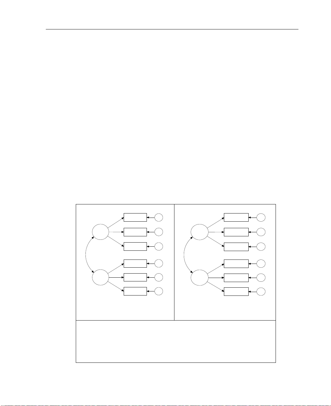
IBM SPSS Amos (Analysis of Moment Structures) is an easy-to-use program for visual SEM. With Amos, you can quickly specify, view, and modify your model graphically using simple drawing tools. Then you can assess your model’s fit, make any modifications, and print out a publication-quality graphic of your final model. Simply specify the model graphically (left). Amos quickly performs the computations and displays the results (right).

Chapter 1

Structural equation modeling (SEM) is sometimes thought of as esoteric and difficult to learn and use. This is incorrect. Indeed, the growing importance of SEM in data analysis is largely due to its ease of use. SEM opens the door for nonstatisticians to solve estimation and hypothesis testing problems that once would have required the services of a specialist.

IBM SPSS Amos was originally designed as a tool for teaching this powerful and fundamentally simple method. For this reason, every effort was made to see that it is easy to use. Amos integrates an easy-to-use graphical interface with an advanced computing engine for SEM. The publication-quality path diagrams of Amos provide a clear representation of models for students and fellow researchers. The numeric methods implemented in Amos are among the most effective and reliable available.

Featured Methods

Amos provides the following methods for estimating structural equation models:

 Maximum likelihood

 Unweighted least squares

 Generalized least squares

 Browne’s asymptotically distribution-free criterion

 Scale-free least squares

 Bayesian estimation

IBM SPSS Amos goes well beyond the usual capabilities found in other structural equation modeling programs. When confronted with missing data, Amos performs state-of-the-art estimation by full information maximum likelihood instead of relying on ad-hoc methods like listwise or pairwise deletion, or mean imputation. The program can analyze data from several populations at once. It can also estimate means for exogenous variables and intercepts in regression equations.

The program makes bootstrapped standard errors and confidence intervals available for all parameter estimates, effect estimates, sample means, variances, covariances, and correlations. It also implements percentile intervals and bias-corrected percentile intervals (Stine, 1989), as well as Bollen and Stine’s (1992) bootstrap approach to model testing.

Multiple models can be fitted in a single analysis. Amos examines every pair of models in which one model can be obtained by placing restrictions on the parameters of the other. The program reports several statistics appropriate for comparing such

models. It provides a test of univariate normality for each observed variable as well as a test of multivariate normality and attempts to detect outliers.

IBM SPSS Amos accepts a path diagram as a model specification and displays parameter estimates graphically on a path diagram. Path diagrams used for model specification and those that display parameter estimates are of presentation quality. They can be printed directly or imported into other applications such as word processors, desktop publishing programs, and general-purpose graphics programs.

About the Tutorial

The tutorial is designed to get you up and running with Amos Graphics. It covers some of the basic functions and features and guides you through your first Amos analysis.

Once you have worked through the tutorial, you can learn about more advanced functions using the online Help, or you can continue working through the examples to get a more extended introduction to structural modeling with IBM SPSS Amos.

Introduction

About the Examples

Many people like to learn by doing. Knowing this, we have developed many examples that quickly demonstrate practical ways to use IBM SPSS Amos. The initial examples introduce the basic capabilities of Amos as applied to simple problems. You learn which buttons to click, how to access the several supported data formats, and how to maneuver through the output. Later examples tackle more advanced modeling problems and are less concerned with program interface issues.

Examples 1 through 4 show how you can use Amos to do some conventional analyses—analyses that could be done using a standard statistics package. These examples show a new approach to some familiar problems while also demonstrating all of the basic features of Amos. There are sometimes good reasons for using Amos to do something simple, like estimating a mean or correlation or testing the hypothesis that two means are equal. For one thing, you might want to take advantage of the ability of Amos to handle missing data. Or maybe you want to use the bootstrapping capability of Amos, particularly to obtain confidence intervals.

Examples 5 through 8 illustrate the basic techniques that are commonly used nowadays in structural modeling.

Chapter 1

Example 9 and those that follow demonstrate advanced techniques that have so far not been used as much as they deserve. These techniques include:

 Simultaneous analysis of data from several different populations.

 Estimation of means and intercepts in regression equations.

 Maximum likelihood estimation in the presence of missing data.

 Bootstrapping to obtain estimated standard errors and confidence intervals. Amos

makes these techniques especially easy to use, and we hope that they will become more commonplace.

 Specification searches.

 Bayesian estimation.

 Imputation of missing values.

 Analysis of censored data.

 Analysis of ordered-categorical data.

 Mixture modeling.

Tip: If you have questions about a particular Amos feature, you can always refer to the

extensive online Help provided by the program.

About the Documentation

IBM SPSS Amos 21 comes with extensive documentation, including an online Help system, this user’s guide, and advanced reference material for Amos Basic and the Amos API (Application Programming Interface). If you performed a typical installation, you can find the IBM SPSS Amos 21 Programming Reference Guide in the following location: C:\Program Files\IBM\SPSS\Amos\21\Documentation\Programming Reference.pdf.

Other Sources of Information

Although this user’s guide contains a good bit of expository material, it is not by any means a complete guide to the correct and effective use of structural modeling. Many excellent SEM textbooks are available.



Structural Equation Modeling: A Multidisciplinary Journal contains methodological articles as well as applications of structural modeling. It is published by Taylor and Francis (http://www.tandf.co.uk).

 Carl Ferguson and Edward Rigdon established an electronic mailing list called

Semnet to provide a forum for discussions related to structural modeling. You can find information about subscribing to Semnet at www.gsu.edu/~mkteer/semnet.html.

Acknowledgements

Many users of previous versions of Amos provided valuable feedback, as did many users who tested the present version. Torsten B. Neilands wrote Examples 26 through 31 in this User’s Guide with contributions by Joseph L. Schafer. Eric Loken reviewed Examples 32 and 33. He also provided valuable insights into mixture modeling as well as important suggestions for future developments in Amos.

A last word of warning: While Amos Development Corporation has engaged in extensive program testing to ensure that Amos operates correctly, all complicated software, Amos included, is bound to contain some undetected bugs. We are committed to correcting any program errors. If you believe you have encountered one, please report it to technical support.

Introduction

James L. Arbuckle

Tutorial: Getting Started with Amos Graphics

Introduction

Remember your first statistics class when you sweated through memorizing formulas and laboriously calculating answers with pencil and paper? The professor had you do this so that you would understand some basic statistical concepts. Later, you discovered that a calculator or software program could do all of these calculations in a split second.

This tutorial is a little like that early statistics class. There are many shortcuts to drawing and labeling path diagrams in Amos Graphics that you will discover as you work through the examples in this user’s guide or as you refer to the online help. The intent of this tutorial is to simply get you started using Amos Graphics. It will cover some of the basic functions and features of IBM SPSS Amos and guide you through your first Amos analysis.

Once you have worked through the tutorial, you can learn about more advanced functions from the online help, or you can continue to learn incrementally by working your way through the examples.

If you performed a typical installation, you can find the path diagram constructed in this tutorial in this location: C:\Program Files\IBM\SPSS\Amos\21\Tutorial\<language>. The file Startsps.amw uses a data file in SPSS Statistics format. Getstart.amw is the same path diagram but uses data from a Microsoft Excel file.

Chapter

Tip: IBM SPSS Amos 21 provides more than one way to accomplish most tasks. For

all menu commands except Tools > Macro, there is a toolbar button that performs the same task. For many tasks, Amos also provides keyboard shortcuts. The user’s guide

Chapter 2

demonstrates the menu path. For information about the toolbar buttons and keyboard shortcuts, see the online help.

About the Data

Hamilton (1990) provided several measurements on each of 21 states. Three of the measurements will be used in this tutorial:

 Average SAT score

 Per capita income expressed in $1,000 units

 Median education for residents 25 years of age or older

You can find the data in the Tutorial directory within the Excel 8.0 workbook

Hamilton.xls in the worksheet named Hamilton. The data are as follows:

SAT Income Education

899 14.345 12.7 896 16.37 12.6 897 13.537 12.5 889 12.552 12.5 823 11.441 12.2 857 12.757 12.7 860 11.799 12.4 890 10.683 12.5 889 14.112 12.5 888 14.573 12.6 925 13.144 12.6 869 15.281 12.5 896 14.121 12.5 827 10.758 12.2 908 11.583 12.7 885 12.343 12.4 887 12.729 12.3 790 10.075 12.1 868 12.636 12.4 904 10.689 12.6 888 13.065 12.4

Tutorial: Getting Started with Amos Graphics

The following path diagram shows a model for these data:

This is a simple regression model where one observed variable, SAT, is predicted as a

linear combination of the other two observed variables, Education and Income. As with

nearly all empirical data, the prediction will not be perfect. The variable Other represents variables other than Education and Income that affect SAT.

Each single-headed arrow represents a regression weight. The number

1 in the

figure specifies that Other must have a weight of 1 in the prediction of SAT. Some such constraint must be imposed in order to make the model identified, and it is one of the features of the model that must be communicated to Amos.

Launching Amos Graphics

You can launch Amos Graphics in any of the following ways:

 Click Start on the Windows task bar, and choose All Programs > IBM SPSS

Statistics

 Double-click any path diagram (*.amw).

 Drag a path diagram (*.amw) file from Windows Explorer to the Amos Graphics

window.

 Click Start on the Windows task bar, and choose All Programs > IBM SPSS

Statistics

diagram in the View Path Diagrams window.

 From within SPSS Statistics, choose Analyze > IBM SPSS Amos from the menus.

> IBM SPSS Amos 21 > Amos Graphics.

> IBM SPSS Amos 21 > View Path Diagrams. Then double-click a path

Chapter 2

Creating a New Model

E From the menus, choose File > New.

Your work area appears. The large area on the right is where you draw path diagrams. The toolbar on the left provides one-click access to the most frequently used buttons. You can use either the toolbar or menu commands for most operations.

Specifying the Data File

The next step is to specify the file that contains the Hamilton data. This tutorial uses a Microsoft Excel 8.0 (*.xls) file, but Amos supports several common database formats, including SPSS Statistics *.sav files. If you launch Amos from the Add-ons menu in SPSS Statistics, Amos automatically uses the file that is open in SPSS Statistics.

E From the menus, choose File > Data Files.

E In the Data Files dialog box, click File Name.

E Browse to the Tutorial folder. If you performed a typical installation, the path is

C:\Program Files\IBM\SPSS\Amos\21\Tutorial\<language>.

E In the Files of type list, select Excel 8.0 (*.xls).

E Select Hamilton.xls, and then click Open.

E In the Data Files dialog box, click OK.

Tutorial: Getting Started with Amos Graphics

Specifying the Model and Drawing Variables

The next step is to draw the variables in your model. First, you’ll draw three rectangles to represent the observed variables, and then you’ll draw an ellipse to represent the unobserved variable.

E From the menus, choose Diagram > Draw Observed.

E In the drawing area, move your mouse pointer to where you want the Education

rectangle to appear. Click and drag to draw the rectangle. Don’t worry about the exact size or placement of the rectangle because you can change it later.

E Use the same method to draw two more rectangles for Income and SAT.

E From the menus, choose Diagram > Draw Unobserved.

Chapter 2

E In the drawing area, move your mouse pointer to the right of the three rectangles and

click and drag to draw the ellipse.

The model in your drawing area should now look similar to the following:

Naming the Variables

E In the drawing area, right-click the top left rectangle and choose Object Properties from

the pop-up menu.

E Click the Text tab.

E In the Variable name text box, type Education.

E Use the same method to name the remaining variables. Then close the Object

Properties dialog box.

Your path diagram should now look like this:

Drawing Arrows

Now you will add arrows to the path diagram, using the following model as your guide:

Tutorial: Getting Started with Amos Graphics

E From the menus, choose Diagram > Draw Path.

E Click and drag to draw an arrow between Education and SAT.

E Use this method to add each of the remaining single-headed arrows.

E From the menus, choose Diagram > Draw Covariances.

E Click and drag to draw a double-headed arrow between Income and Education. Don’t

worry about the curve of the arrow because you can adjust it later.

Chapter 2

Constraining a Parameter

To identify the regression model, you must define the scale of the latent variable Other.

You can do this by fixing either the variance of Other or the path coefficient from Other to SAT at some positive value. The following shows you how to fix the path coefficient at unity (1).

E In the drawing area, right-click the arrow between Other and SAT and choose Object

Properties

E Click the Parameters tab.

E In the Regression weight text box, type 1.

from the pop-up menu.

E Close the Object Properties dialog box.

There is now a

1 above the arrow between Other and SAT. Your path diagram is now

complete, other than any changes you may wish to make to its appearance. It should look something like this:

Tutorial: Getting Started with Amos Graphics

Altering the Appearance of a Path Diagram

You can change the appearance of your path diagram by moving and resizing objects. These changes are visual only; they do not affect the model specification.

To Move an Object

E From the menus, choose Edit > Move.

E In the drawing area, click and drag the object to its new location.

To Reshape an Object or Double-Headed Arrow

E From the menus, choose Edit > Shape of Object.

E In the drawing area, click and drag the object until you are satisfied with its size and

shape.

To Delete an Object

E From the menus, choose Edit > Erase.

E In the drawing area, click the object you wish to delete.

Chapter 2

To Undo an Action

E From the menus, choose Edit > Undo.

To Redo an Action

E From the menus, choose Edit > Redo.

Setting Up Optional Output

Some of the output in Amos is optional. In this step, you will choose which portions of the optional output you want Amos to display after the analysis.

E From the menus, choose View > Analysis Properties.

E Click the Output tab.

E Select the Minimization history, Standardized estimates, and Squared multiple correlations

check boxes.

Tutorial: Getting Started with Amos Graphics

Close the Analysis Properties dialog box.

Chapter 2

Performing the Analysis

The only thing left to do is perform the calculations for fitting the model. Note that in order to keep the parameter estimates up to date, you must do this every time you change the model, the data, or the options in the Analysis Properties dialog box.

E From the menus, click Analyze > Calculate Estimates.

E Because you have not yet saved the file, the Save As dialog box appears. Type a name

for the file and click Save.

Amos calculates the model estimates. The panel to the left of the path diagram displays a summary of the calculations.

Viewing Output

When Amos has completed the calculations, you have two options for viewing the output: text and graphics.

To View Text Output

E From the menus, choose View > Text Output.

The tree diagram in the upper left pane of the Amos Output window allows you to choose a portion of the text output for viewing.

E Click Estimates to view the parameter estimates.

Tutorial: Getting Started with Amos Graphics

To View Graphics Output

E Click the Show the output path diagram button .

E In the Parameter Formats pane to the left of the drawing area, click Standardized

estimates.

Chapter 2

Your path diagram now looks like this:

The value 0.49 is the correlation between Education and Income. The values 0.72 and

0.11 are standardized regression weights. The value 0.60 is the squared multiple correlation of SAT with Education and Income.

E In the Parameter Formats pane to the left of the drawing area, click Unstandardized

estimates

Your path diagram should now look like this:

Printing the Path Diagram

E From the menus, choose File > Print.

The Print dialog box appears.

E Click Print.

Copying the Path Diagram

Tutorial: Getting Started with Amos Graphics

Amos Graphics lets you easily export your path diagram to other applications such as Microsoft Word.

E From the menus, choose Edit > Copy (to Clipboard).

E Switch to the other application and use the Paste function to insert the path diagram.

Amos Graphics exports only the diagram; it does not export the background.

Copying Text Output

E In the Amos Output window, select the text you want to copy.

E Right-click the selected text, and choose Copy from the pop-up menu.

E Switch to the other application and use the Paste function to insert the text.

Estimating Variances and Covariances

Introduction

This example shows you how to estimate population variances and covariances. It also discusses the general format of Amos input and output.

Example

About the Data

Attig (1983) showed 40 subjects a booklet containing several pages of advertisements. Then each subject was given three memory performance tests.

Test Explanation

recall

cued

place

Attig repeated the study with the same 40 subjects after a training exercise intended to improve memory performance. There were thus three performance measures before training and three performance measures after training. In addition, she recorded scores on a vocabulary test, as well as age, sex, and level of education. Attig’s data files are included in the Examples folder provided by Amos.

The subject was asked to recall as many of the advertisements as possible. The subject’s score on this test was the number of advertisements recalled correctly.

The subject was given some cues and asked again to recall as many of the advertisements as possible. The subject’s score was the number of advertisements recalled correctly.

The subject was given a list of the advertisements that appeared in the booklet and was asked to recall the page location of each one. The subject’s score on this test was the number of advertisements whose location was recalled correctly.

Example 1

Bringing In the Data

E From the menus, choose File > New.

E From the menus, choose File > Data Files.

E In the Data Files dialog box, click File Name.

E Browse to the Examples folder. If you performed a typical installation, the path is

C:\Program Files\IBM\SPSS\Amos\21\Examples\<language>.

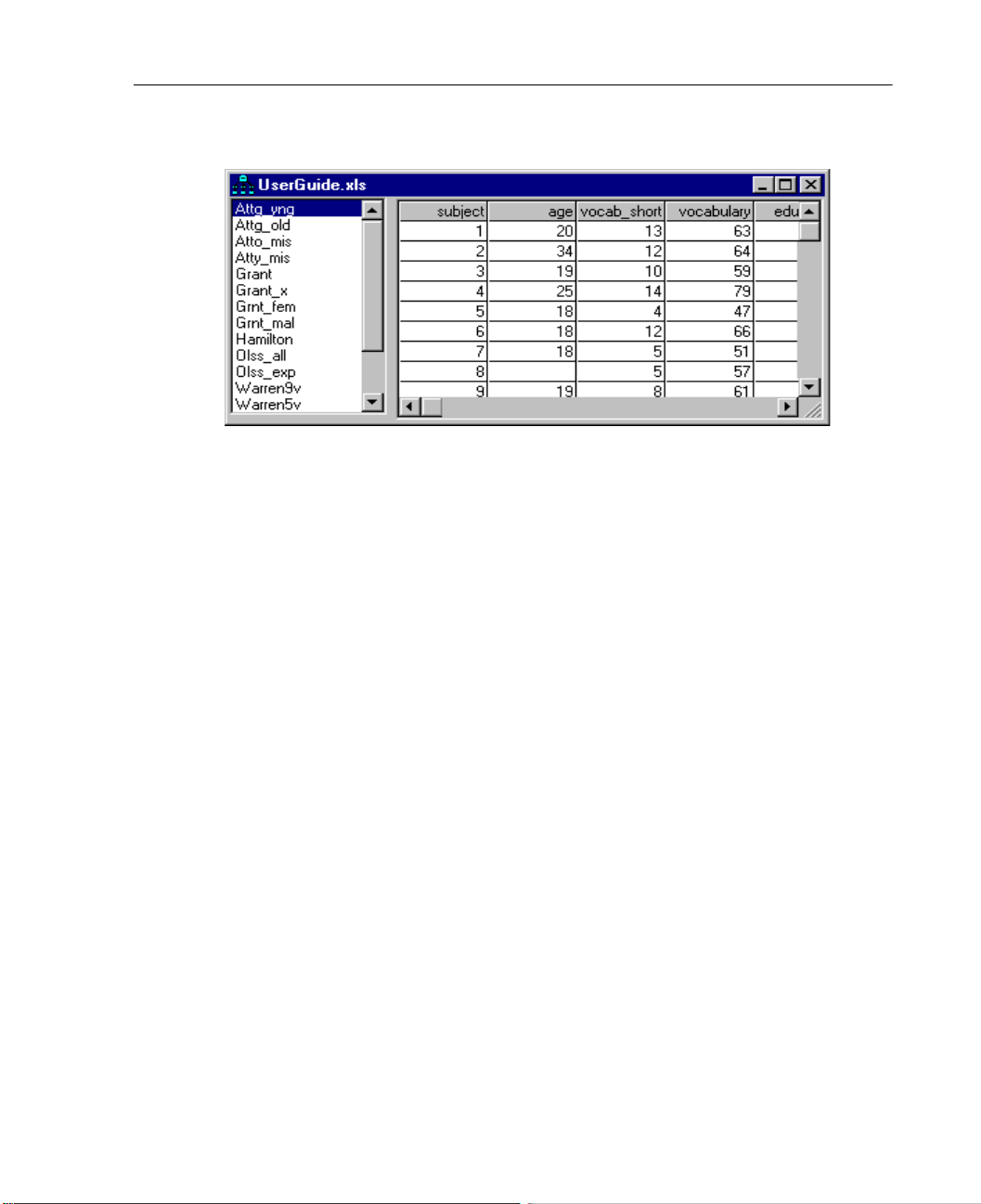
E In the Files of type list, select Excel 8.0 (*.xls), select UserGuide.xls, and then click

Open.

E In the Data Files dialog box, click OK.

Amos displays a list of worksheets in the UserGuide workbook. The worksheet Attg_yng contains the data for this example.

E In the Select a Data Table dialog box, select Attg_yng, then click View Data.

The Excel worksheet for the Attg_yng data file opens.

Estimating Variances and Covariances

As you scroll across the worksheet, you will see all of the test variables from the Attig study. This example uses only the following variables: recall1 (recall pretest), recall2 (recall posttest), place1 (place recall pretest), and place2 (place recall posttest).

E After you review the data, close the data window.

E In the Data Files dialog box, click OK.

Analyzing the Data

In this example, the analysis consists of estimating the variances and covariances of the recall and place variables before and after training.

Specifying the Model

E From the menus, choose Diagram > Draw Observed.

E In the drawing area, move your mouse pointer to where you want the first rectangle to

appear. Click and drag to draw the rectangle.

E From the menus, choose Edit > Duplicate.

E Click and drag a duplicate from the first rectangle. Release the mouse button to

position the duplicate.

Example 1

E Create two more duplicate rectangles until you have four rectangles side by side.

Tip: If you want to reposition a rectangle, choose Edit > Move from the menus and drag

the rectangle to its new position.

Naming the Variables

E From the menus, choose View > Variables in Dataset.

The Variables in Dataset dialog box appears.

E Click and drag the variable recall1 from the list to the first rectangle in the drawing

area.

E Use the same method to name the variables recall2, place1, and place2.

E Close the Variables in Dataset dialog box.

Changing the Font

E Right-click a variable and choose Object Properties from the pop-up menu.

The Object Properties dialog box appears.

E Click the Text tab and adjust the font attributes as desired.

Estimating Variances and Covariances

Establishing Covariances

If you leave the path diagram as it is, Amos Graphics will estimate the variances of the four variables, but it will not estimate the covariances between them. In Amos Graphics, the rule is to assume a correlation or covariance of 0 for any two variables that are not connected by arrows. To estimate the covariances between the observed variables, we must first connect all pairs with double-headed arrows.

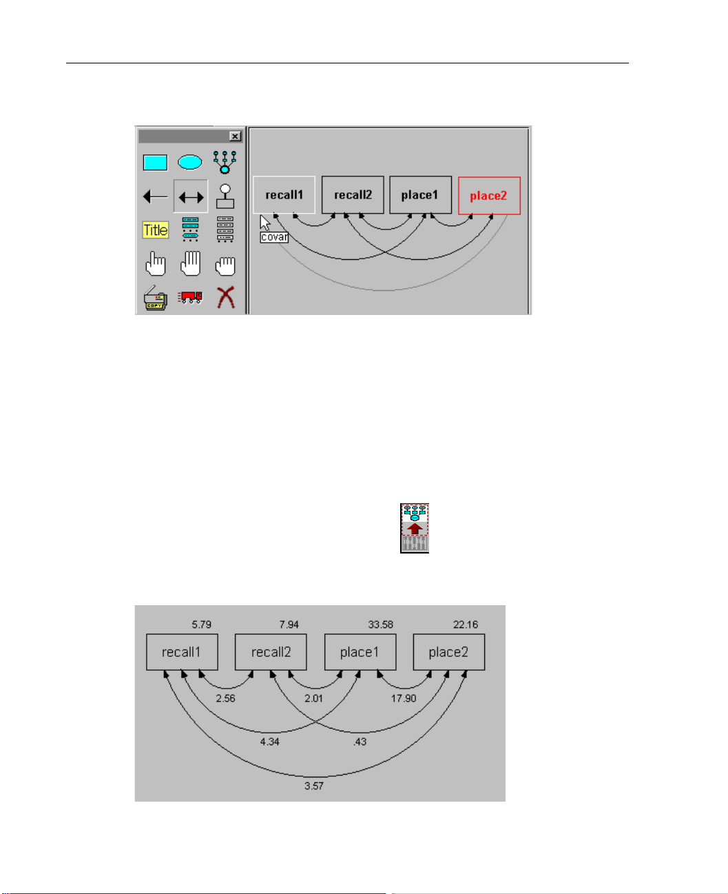
E From the menus, choose Diagram > Draw Covariances.

E Click and drag to draw arrows that connect each variable to every other variable.

Your path diagram should have six double-headed arrows.

Example 1

Performing the Analysis

E From the menus, choose Analyze > Calculate Estimates.

Because you have not yet saved the file, the Save As dialog box appears.

E Enter a name for the file and click Save.

Viewing Graphics Output

E Click the Show the output path diagram button .

Amos displays the output path diagram with parameter estimates.

In the output path diagram, the numbers displayed next to the boxes are estimated variances, and the numbers displayed next to the double-headed arrows are estimated covariances. For example, the variance of recall1 is estimated at 5.79, and that of place1 at 33.58. The estimated covariance between these two variables is 4.34.

Viewing Text Output

E From the menus, choose View > Text Output.

E In the tree diagram in the upper left pane of the Amos Output window, click Estimates.

Estimating Variances and Covariances

The first estimate displayed is of the covariance between recall1 and recall2. The covariance is estimated to be 2.56. Right next to that estimate, in the S.E

. column, is an

estimate of the standard error of the covariance, 1.16. The estimate 2.56 is an

2.56 1.96 1.160 2.56 2.27±=×±

2.20 2.56 1.16⁄=()

p 0.03=

Example 1

observation on an approximately normally distributed random variable centered around the population covariance with a standard deviation of about 1.16, that is, if the assumptions in the section “Distribution Assumptions for Amos Models” on p. 35 are met. For example, you can use these figures to construct a 95% confidence interval on the population covariance by computing . Later, you will see that you can use Amos to estimate many kinds of population parameters besides covariances and can follow the same procedure to set a confidence interval on any one of them.

Next to the standard error, in the

C.R. column, is the critical ratio obtained by

dividing the covariance estimate by its standard error . This ratio is relevant to the null hypothesis that, in the population from which Attig’s 40 subjects came, the covariance between recall1 and recall2 is 0. If this hypothesis is true, and still under the assumptions in the section “Distribution Assumptions for Amos Models” on p. 35, the critical ratio is an observation on a random variable that has an approximate standard normal distribution. Thus, using a significance level of 0.05, any critical ratio that exceeds 1.96 in magnitude would be called significant. In this example, since 2.20 is greater than 1.96, you would say that the covariance between recall1 and recall2 is significantly different from 0 at the 0.05 level.

The P column, to the right of C.R., gives an approximate two-tailed p value for testing the null hypothesis that the parameter value is 0 in the population. The table shows that the covariance between recall1 and recall2 is significantly different from 0 with . The calculation of P assumes that parameter estimates are normally distributed, and it is correct only in large samples. See Appendix A for more information.

The assertion that the parameter estimates are normally distributed is only an approximation. Moreover, the standard errors reported in the S.E. column are only approximations and may not be the best available. Consequently, the confidence interval and the hypothesis test just discussed are also only approximate. This is because the theory on which these results are based is asymptotic. Asymptotic means that it can be made to apply with any desired degree of accuracy, but only by using a sufficiently large sample. We will not discuss whether the approximation is satisfactory with the present sample size because there would be no way to generalize the conclusions to the many other kinds of analyses that you can do with Amos. However, you may want to re-examine the null hypothesis that recall1 and recall2 are uncorrelated, just to see what is meant by an approximate test. We previously concluded that the covariance is significantly different from 0 because 2.20 exceeds

1.96. The p value associated with a standard normal deviate of 2.20 is 0.028 (twotailed), which, of course, is less than 0.05. By contrast, the conventional t statistic (for

Estimating Variances and Covariances

p 0.016=()

example, Runyon and Haber, 1980, p. 226) is 2.509 with 38 degrees of freedom

. In this example, both p values are less than 0.05, so both tests agree in rejecting the null hypothesis at the 0.05 level. However, in other situations, the two p values might lie on opposite sides of 0.05. You might or might not regard this as especially serious—at any rate, the two tests can give different results. There should be no doubt about which test is better. The t test is exact under the assumptions of normality and independence of observations, no matter what the sample size. In Amos, the test based on critical ratio depends on the same assumptions; however, with a finite sample, the test is only approximate.

Note: For many interesting applications of Amos, there is no exact test or exact standard

error or exact confidence interval available.

On the bright side, when fitting a model for which conventional estimates exist, maximum likelihood point estimates (for example, the numbers in the Estimate column) are generally identical to the conventional estimates.

E Now click Notes for Model in the upper left pane of the Amos Output window.

The following table plays an important role in every Amos analysis:

Number of distinct sample moments: 10

Number of distinct parameters to be estimated: 10

Degrees of freedom (10 – 10): 0

Example 1

The Number of distinct sample moments referred to are sample means, variances, and covariances. In most analyses, including the present one, Amos ignores means, so that the sample moments are the sample variances of the four variables, recall1, recall2, place1, and place2, and their sample covariances. There are four sample variances and six sample covariances, for a total of 10 sample moments.

The Number of distinct parameters to be estimated are the corresponding population variances and covariances. There are, of course, four population variances and six population covariances, which makes 10 parameters to be estimated.

The Degrees of freedom is the amount by which the number of sample moments exceeds the number of parameters to be estimated. In this example, there is a one-toone correspondence between the sample moments and the parameters to be estimated, so it is no accident that there are zero degrees of freedom.

As we will see beginning with Example 2, any nontrivial null hypothesis about the parameters reduces the number of parameters that have to be estimated. The result will be positive degrees of freedom. For now, there is no null hypothesis being tested. Without a null hypothesis to test, the following table is not very interesting:

Chi-square = 0.00 Degrees of freedom = 0 Probability level cannot be computed

If there had been a hypothesis under test in this example, the chi-square value would have been a measure of the extent to which the data were incompatible with the hypothesis. A chi-square value of 0 would ordinarily indicate no departure from the null hypothesis. But in the present example, the 0 value for degrees of freedom and the 0 chi-square value merely reflect the fact that there was no null hypothesis in the first place.

Minimum was achieved

This line indicates that Amos successfully estimated the variances and covariances. Sometimes structural modeling programs like Amos fail to find estimates. Usually, when Amos fails, it is because you have posed a problem that has no solution, or no unique solution. For example, if you attempt maximum likelihood estimation with observed variables that are linearly dependent, Amos will fail because such an analysis cannot be done in principle. Problems that have no unique solution are discussed elsewhere in this user’s guide under the subject of identifiability. Less commonly, Amos can fail because an estimation problem is just too difficult. The possibility of such failures is generic to programs for analysis of moment structures. Although the computational method used by Amos is highly effective, no computer program that does the kind of analysis that Amos does can promise success in every case.

Optional Output

So far, we have discussed output that Amos generates by default. You can also request additional output.

Calculating Standardized Estimates

You may be surprised to learn that Amos displays estimates of covariances rather than correlations. When the scale of measurement is arbitrary or of no substantive interest, correlations have more descriptive meaning than covariances. Nevertheless, Amos and similar programs insist on estimating covariances. Also, as will soon be seen, Amos provides a simple method for testing hypotheses about covariances but not about correlations. This is mainly because it is easier to write programs that way. On the other hand, it is not hard to derive correlation estimates after the relevant variances and covariances have been estimated. To calculate standardized estimates:

E From the menus, choose View > Analysis Properties.

Estimating Variances and Covariances

E In the Analysis Properties dialog box, click the Output tab.

E Select the Standardized estimates check box.

E Close the Analysis Properties dialog box.

Example 1

Rerunning the Analysis

Because you have changed the options in the Analysis Properties dialog box, you must rerun the analysis.

E From the menus, choose Analyze > Calculate Estimates.

E Click the Show the output path diagram button.

E In the Parameter Formats pane to the left of the drawing area, click Standardized

estimates

Viewing Correlation Estimates as Text Output

E From the menus, choose View > Text Output.

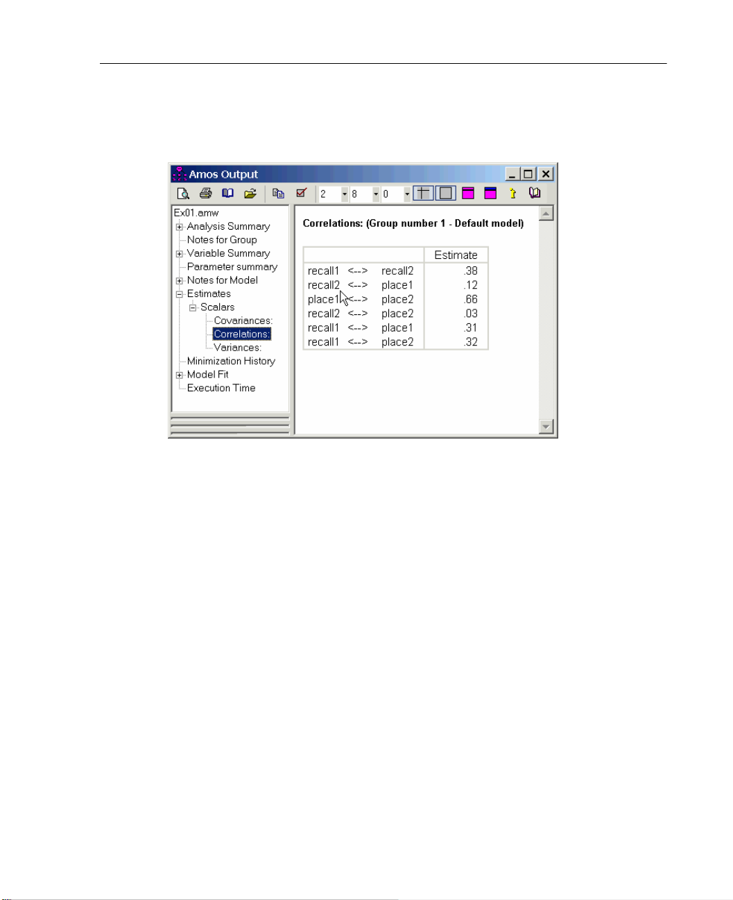
Estimating Variances and Covariances

In the tree diagram in the upper left pane of the Amos Output window, expand

Estimates, Scalars, and then click Correlations.

Distribution Assumptions for Amos Models

Hypothesis testing procedures, confidence intervals, and claims for efficiency in maximum likelihood or generalized least-squares estimation depend on certain assumptions. First, observations must be independent. For example, the 40 young people in the Attig study have to be picked independently from the population of young people. Second, the observed variables must meet some distributional requirements. If the observed variables have a multivariate normal distribution, that will suffice. Multivariate normality of all observed variables is a standard distribution assumption in many structural equation modeling and factor analysis applications.

There is another, more general, situation under which maximum likelihood estimation can be carried out. If some exogenous variables are fixed (that is, they are either known beforehand or measured without error), their distributions may have any shape, provided that:

 For any value pattern of the fixed variables, the remaining (random) variables have

a (conditional) normal distribution.

 The (conditional) variance-covariance matrix of the random variables is the same

for every pattern of the fixed variables.

Example 1

 The (conditional) expected values of the random variables depend linearly on the

values of the fixed variables.

A typical example of a fixed variable would be an experimental treatment, classifying respondents into a study group and a control group, respectively. It is all right that treatment is non-normally distributed, as long as the other exogenous variables are normally distributed for study and control cases alike, and with the same conditional variance-covariance matrix. Predictor variables in regression analysis (see Example 4) are often regarded as fixed variables.

Many people are accustomed to the requirements for normality and independent observations, since these are the usual requirements for many conventional procedures. However, with Amos, you have to remember that meeting these requirements leads only to asymptotic conclusions (that is, conclusions that are approximately true for large samples).

Modeling in VB.NET

It is possible to specify and fit a model by writing a program in VB.NET or in C#. Writing programs is an alternative to using Amos Graphics to specify a model by drawing its path diagram. This section shows how to write a VB.NET program to perform the analysis of Example 1. A later section explains how to do the same thing in C#.

Amos comes with its own built-in editor for VB.NET and C# programs. It is accessible from the Windows Start menu. To begin Example 1 using the built-in editor:

E From the Windows Start menu, choose All Programs > IBM SPSS Statistics >

IBM SPSS Amos 21 > Program Editor.

E In the Program Editor window, choose File > New VB Program.

Estimating Variances and Covariances

E Enter the VB.NET code for specifying and fitting the model in place of the ‘Your code

goes here

comment. The following figure shows the program editor after the complete

program has been entered.

Note: The Examples directory contains all of the pre-written examples.

Example 1

E From the Program Editor menus, choose File > Open.

E Select the file Ex01.vb in the \Amos\21\Examples\<language> directory.

To open the VB.NET file for the present example:

The following table gives a line-by-line explanation of the program.

Program Statement Explanation

Declares Sem as an object of type

Dim Sem As New AmosEngine

Sem.TextOutput

Sem.BeginGroup …

Sem.AStructure("recall1") Sem.AStructure("recall2") Sem.AStructure("place1") Sem.AStructure("place2")

Sem.FitModel()

Sem.Dispose()

Try/Finally/End Try

AmosEngine. The methods and properties of

the Sem object are used to specify and fit the model.

Creates an output file containing the results of the analysis. At the end of the analysis, the contents of the output file are displayed in a separate window.

Begins the model specification for a single group (that is, a single population). This line also specifies that the Attg_yng worksheet in the Excel workbook UserGuide.xls contains the input data.

Sem.AmosDir() is the location of the

Amos program directory. Specifies the model. The four AStructure

statements declare the variances of recall1, recall2, place1, and place2 to be free parameters. The other eight variables in the Attg_yng data file are left out of this analysis. In an Amos program (but not in Amos Graphics), observed exogenous variables are assumed by default to be correlated, so that Amos will estimate the six covariances among the four variables.

Fits the model. Releases resources used by the Sem object. It is

particularly important for your program to use an AmosEngine object’s

Dispose method before

creating another AmosEngine object. A process is allowed only one instance of an AmosEngine object at a time.

The Try block guarantees that the Dispose method will be called even if an error occurs during program execution.

E To perform the analysis, from the menus, choose File > Run.

Generating Additional Output

Some AmosEngine methods generate additional output. For example, the Standardized method displays standardized estimates. The following figure shows the use of the

Standardized method:

Estimating Variances and Covariances

Modeling in C#

Writing an Amos program in C# is similar to writing one in VB.NET. To start a new C# program, in the built-in program editor of Amos:

E Choose File > New C# Program (rather than File > New VB Program).

E Choose File > Open to open Ex01.cs, which is a C# version of the VB.NET program

Ex01.vb.

Example 1

Other Program Development Tools

The built-in program editor in Amos is used throughout this user’s guide for writing and executing Amos programs. However, you can use the development tool of your choice. The Examples folder contains a VisualStudio subfolder where you can find Visual Studio VB.NET and C# solutions for Example 1.

Testing Hypotheses

Introduction

This example demonstrates how you can use Amos to test simple hypotheses about variances and covariances. It also introduces the chi-square test for goodness of fit and elaborates on the concept of degrees of freedom.

Example

About the Data

We will use Attig’s (1983) spatial memory data, which were described in Example 1. We will also begin with the same path diagram as in Example 1. To demonstrate the ability of Amos to use different data formats, this example uses a data file in SPSS Statistics format instead of an Excel file.

Parameters Constraints

The following is the path diagram from Example 1. We can think of the variable objects as having small boxes nearby (representing the variances) that are filled in once Amos has estimated the parameters.

Example 2

You can fill these boxes yourself instead of letting Amos fill them.

Constraining Variances

Suppose you want to set the variance of recall1 to 6 and the variance of recall2 to 8.

E In the drawing area, right-click recall1 and choose Object Properties from the pop-up

menu.

E Click the Parameters tab.

E In the Variance text box, type 6.

E With the Object Properties dialog box still open, click recall2 and set its variance to 8.

Close the dialog box.

The path diagram displays the parameter values you just specified.

This is not a very realistic example because the numbers 6 and 8 were just picked out of the air. Meaningful parameter constraints must have some underlying rationale, perhaps being based on theory or on previous analyses of similar data.

Specifying Equal Parameters

Testing Hypotheses

Sometimes you will be interested in testing whether two parameters are equal in the population. You might, for example, think that the variances of recall1 and recall2 might be equal without having a particular value for the variances in mind. To investigate this possibility, do the following:

E In the drawing area, right-click recall1 and choose Object Properties from the pop-up

menu.

E Click the Parameters tab.

E In the Variance text box, type v_recall.

E Click recall2 and label its variance as v_recall.

E Use the same method to label the place1 and place2 variances as v_place.

It doesn’t matter what label you use. The important thing is to enter the same label for each variance you want to force to be equal. The effect of using the same label is to

Example 2

require both of the variances to have the same value without specifying ahead of time what that value is.

Benefits of Specifying Equal Parameters

Before adding any further constraints on the model parameters, let’s examine why we might want to specify that two parameters, like the variances of recall1 and recall2 or place1 and place2, are equal. Here are two benefits:

 If you specify that two parameters are equal in the population and if you are correct

in this specification, then you will get more accurate estimates, not only of the parameters that are equal but usually of the others as well. This is the only benefit if you happen to know that the parameters are equal.

 If the equality of two parameters is a mere hypothesis, requiring their estimates to

be equal will result in a test of that hypothesis.

Constraining Covariances

Your model may also include restrictions on parameters other than variances. For example, you may hypothesize that the covariance between recall1 and place1 is equal to the covariance between recall2 and place2. To impose this constraint:

E In the drawing area, right-click the double-headed arrow that connects recall1 and

place1, and choose

E Click the Parameters tab.

E In the Covariance text box, type a non-numeric string such as cov_rp.

E Use the same method to set the covariance between recall2 and place2 to cov_rp.

Object Properties from the pop-up menu.

Testing Hypotheses

Moving and Formatting Objects

While a horizontal layout is fine for small examples, it is not practical for analyses that are more complex. The following is a different layout of the path diagram on which we’ve been working:

Example 2

You can use the following tools to rearrange your path diagram until it looks like the one above:

 To move objects, choose Edit > Move from the menus, and then drag the object to

 To copy formatting from one object to another, choose Edit > Drag Properties from

For more information about the Drag Properties feature, refer to online help.

Data Input

This example uses a data file in SPSS Statistics format. If you have SPSS Statistics installed, you can view the data as you load it. Even if you don’t have SPSS Statistics installed, Amos will still read the data.

E From the menus, choose File > Data Files.

its new location. You can also use the

Move button to drag the endpoints of arrows.

the menus, select the properties you wish to apply, and then drag from one object to another.

E In the Data Files dialog box, click File Name.

E Browse to the Examples folder. If you performed a typical installation, the path is

C:\Program Files\IBM\SPSS\Amos\21\Examples\<language>.

E In the Files of type list, select SPSS Statistics (*.sav), click Attg_yng, and then click

Open.

E If you have SPSS Statistics installed, click the View Data button in the Data Files dialog

box. An SPSS Statistics window opens and displays the data.

Review the data and close the data view.

E In the Data Files dialog box, click OK.

Performing the Analysis

E From the menus, choose Analyze > Calculate Estimates.

E In the Save As dialog box, enter a name for the file and click Save.

Amos calculates the model estimates.

Viewing Text Output

E From the menus, choose View > Text Output.

E To view the parameter estimates, click Estimates in the tree diagram in the upper left

pane of the Amos Output window.

Testing Hypotheses

10 7 3=–

Example 2

E Now click Notes for Model in the upper left pane of the Amos Output window.

You can see that the parameters that were specified to be equal do have equal estimates. The standard errors here are generally smaller than the standard errors obtained in Example 1. Also, because of the constraints on the parameters, there are now positive degrees of freedom.

While there are still 10 sample variances and covariances, the number of parameters to be estimated is only seven. Here is how the number seven is arrived at: The variances of recall1 and recall2, labeled v_recall, are constrained to be equal, and thus count as

a single parameter. The variances of place1 and place2 (labeled v_place) count as

another single parameter. A third parameter corresponds to the equal covariances recall1 <> place1 and recall2 <> place2 (labeled cov_rp). These three parameters, plus the four unlabeled, unrestricted covariances, add up to seven parameters that have to be estimated.

The degrees of freedom ( ) may also be thought of as the number of constraints placed on the original 10 variances and covariances.

Optional Output

The output we just discussed is all generated by default. You can also request additional output:

E From the menus, choose View > Analysis Properties.

E Click the Output tab.

E Ensure that the following check boxes are selected: Minimization history, Standardized

estimates

, Sample moments, Implied moments, and Residual moments.

Testing Hypotheses

E From the menus, choose Analyze > Calculate Estimates.

Amos recalculates the model estimates.

Covariance Matrix Estimates

E To see the sample variances and covariances collected into a matrix, choose View > Text

from the menus.

Output

E Click Sample Moments in the tree diagram in the upper left corner of the Amos Output

window.

Example 2

E In the tree diagram, expand Estimates and then click Matrices.

The following is the sample covariance matrix:

The following is the matrix of implied covariances:

Note the differences between the sample and implied covariance matrices. Because the model imposes three constraints on the covariance structure, the implied variances and covariances are different from the sample values. For example, the sample variance of place1 is 33.58, but the implied variance is 27.53. To obtain a matrix of residual covariances (sample covariances minus implied covariances), put a check mark next to

Residual moments on the Output tab and repeat the analysis.

The following is the matrix of residual covariances:

Testing Hypotheses

Displaying Covariance and Variance Estimates on the Path Diagram

As in Example 1, you can display the covariance and variance estimates on the path diagram.

E Click the Show the output path diagram button.

E In the Parameter Formats pane to the left of the drawing area, click Unstandardized

estimates

clicking Standardized estimates.

The following is the path diagram showing correlations:

. Alternatively, you can request correlation estimates in the path diagram by

Labeling Output

It may be difficult to remember whether the displayed values are covariances or correlations. To avoid this problem, you can use Amos to label the output.

E Open the file Ex02.amw.

E Right-click the caption at the bottom of the path diagram, and choose Object Properties

from the pop-up menu.

E Click the Text tab.

Example 2

Notice the word \format in the bottom line of the figure caption. Words that begin with a backward slash, like information about the currently displayed model. The text macro \format will be replaced by the heading Model Specification, Unstandardized estimates, or Standardized estimates, depending on which version of the path diagram is displayed.

\format, are called text macros. Amos replaces text macros with

Hypothesis Testing

The implied covariances are the best estimates of the population variances and covariances under the null hypothesis. (The null hypothesis is that the parameters required to have equal estimates are truly equal in the population.) As we know from Example 1, the sample covariances are the best estimates obtained without making any assumptions about the population values. A comparison of these two matrices is relevant to the question of whether the null hypothesis is correct. If the null hypothesis is correct, both the implied and sample covariances are maximum likelihood estimates of the corresponding population values (although the implied covariances are better estimates). Consequently, you would expect the two matrices to resemble each other. On the other hand, if the null hypothesis is wrong, only the sample covariances are

Testing Hypotheses

maximum likelihood estimates, and there is no reason to expect them to resemble the implied covariances.

The chi-square statistic is an overall measure of how much the implied covariances

differ from the sample covariances.

Chi-square = 6.276 Degrees of freedom = 3 Probability level = 0.099

In general, the more the implied covariances differ from the sample covariances, the bigger the chi-square statistic will be. If the implied covariances had been identical to the sample covariances, as they were in Example 1, the chi-square statistic would have been 0. You can use the chi-square statistic to test the null hypothesis that the parameters required to have equal estimates are really equal in the population. However, it is not simply a matter of checking to see if the chi-square statistic is 0. Since the implied covariances and the sample covariances are merely estimates, you can’t expect them to be identical (even if they are both estimates of the same population covariances). Actually, you would expect them to differ enough to produce a chi-square in the neighborhood of the degrees of freedom, even if the null hypothesis is true. In other words, a chi-square value of 3 would not be out of the ordinary here, even with a true null hypothesis. You can say more than that: If the null hypothesis is true, the chisquare value (6.276) is a single observation on a random variable that has an approximate chi-square distribution with three degrees of freedom. The probability is about 0.099 that such an observation would be as large as 6.276. Consequently, the evidence against the null hypothesis is not significant at the 0.05 level.

Displaying Chi-Square Statistics on the Path Diagram

You can get the chi-square statistic and its degrees of freedom to appear in a figure caption on the path diagram using the text macros text macros with the numeric values of the chi-square statistic and its degrees of freedom. You can use the text macro

\p to display the corresponding right-tail

probability under the chi-square distribution.

E From the menus, choose Diagram > Figure Caption.

E Click the location on the path diagram where you want the figure caption to appear.

The Figure Caption dialog box appears.

\cmin and \df. Amos replaces these

Example 2

E In the Figure Caption dialog box, enter a caption that includes the \cmin, \df, and \p text

macros, as follows:

When Amos displays the path diagram containing this caption, it appears as follows:

Modeling in VB.NET

The following program fits the constrained model of Example 2:

Testing Hypotheses

Example 2

This table gives a line-by-line explanation of the program:

Program Statement Explanation

Declares Sem as an object of type

Dim Sem As New AmosEngine

Sem.TextOutput

Sem.Standardized() Sem.ImpliedMoments() Sem.SampleMoments() Sem.ResidualMoments()

Sem.BeginGroup …

Sem.AStructure("recall1 (v_recall)") Sem.AStructure("recall2 (v_recall)") Sem.AStructure("place1 (v_place)") Sem.AStructure("place2 (v_place)") Sem.AStructure("recall1 <> place1 (cov_rp)") Sem.AStructure("recall2 <> place2 (cov_rp)")

Sem.FitModel()

Sem.Dispose()

Try/Finally/End Try

AmosEngine. The methods and

properties of the Sem object are used to specify and fit the model.

Creates an output file containing the results of the analysis. At the end of the analysis, the contents of the output file are displayed in a separate window.

Displays standardized estimates, implied covariances, sample covariances, and residual covariances.

Begins the model specification for a single group (that is, a single population). This line also specifies that the SPSS Statistics file Attg_yng.sav contains the input data. is the location of the Amos program directory.

Specifies the model. The first four

AStructure statements constrain the

variances of the observed variables through the use of parameter names in parentheses. Recall1 and recall2 are required to have the same variance because both variances are labeled

v_recall. The variances of place1 and place2 are similarly constrained to be

equal. Each of the last two lines represents a covariance. The two covariances are both named cov_rp. Consequently, those covariances are constrained to be equal.

Fits the model. Releases resources used by the Sem

object. It is particularly important for your program to use an AmosEngine object’s

Dispose method before creating

another AmosEngine object. A process is allowed to have only one instance of an AmosEngine object at a time.

This Try block guarantees that the

Dispose method will be called even if an

error occurs during program execution.

Sem.AmosDir()

AStructure

To perform the analysis, from the menus, choose File > Run.

Timing Is Everything

The AStructure lines must appear after BeginGroup; otherwise, Amos will not recognize that the variables named in the attg_yng.sav dataset.

In general, the order of statements matters in an Amos program. In organizing an

Amos program, AmosEngine methods can be divided into three general groups

Group 1 — Declarative Methods

This group contains methods that tell Amos what results to compute and display.

TextOutput is a Group 1 method, as are Standardized, ImpliedMoments, SampleMoments,

and ResidualMoments. Many other Group 1 methods that are not used in this example are documented in the Amos 21 Programming Reference Guide.

Group 2 — Data and Model Specification Methods

Testing Hypotheses

AStructure lines are observed variables in the

This group consists of data description and model specification commands.

BeginGroup and AStructure are Group 2 methods. Others are documented in the Amos

21 Programming Reference Guide.

Group 3 — Methods for Retrieving Results

These are commands to…well, retrieve results. So far, we have not used any Group 3 methods. Examples using Group 3 methods are given in the Amos 21 Programming Reference Guide.

Tip: When you write an Amos program, it is important to pay close attention to the

order in which you call the Amos engine methods. The rule is that groups must appear in order: Group 1, then Group 2, and finally Group 3.

For more detailed information about timing rules and a complete listing of methods and their group membership, see the Amos 21 Programming Reference Guide.

1 There is also a fourth special group, consisting of only the Initialize Method. If the optional Initialize Method is used, it must come before the Group 1 methods.

More Hypothesis Testing

Introduction

This example demonstrates how to test the null hypothesis that two variables are uncorrelated, reinforces the concept of degrees of freedom, and demonstrates, in a concrete way, what is meant by an asymptotically correct test.

Example

About the Data

For this example, we use the group of older subjects from Attig’s (1983) spatial memory study and the two variables age and vocabulary. We will use data formatted as a tab-delimited text file.

Bringing In the Data

E From the menus, choose File > New.

E From the menus, choose File > Data Files.

E In the Data Files dialog box, select File Name.

E Browse to the Examples folder. If you performed a typical installation, the path is

C:\Program Files\IBM\SPSS\Amos\21\Examples\<language>.

Example 3

E In the Files of type list, select Text (*.txt), select Attg_old.txt, and then click Open.

E In the Data Files dialog box, click OK.

Testing a Hypothesis That Two Variables Are Uncorrelated

Among Attig’s 40 old subjects, the sample correlation between age and vocabulary is –0.09 (not very far from 0). Is this correlation nevertheless significant? To find out, we will test the null hypothesis that, in the population from which these 40 subjects came, the correlation between age and vocabulary is 0. We will do this by estimating the variance-covariance matrix under the constraint that age and vocabulary are uncorrelated.

Specifying the Model

Begin by drawing and naming the two observed variables, age and vocabulary, in the path diagram, using the methods you learned in Example 1.

Amos provides two ways to specify that the covariance between age and vocabulary

is 0. The most obvious way is simply to not draw a double-headed arrow connecting the two variables. The absence of a double-headed arrow connecting two exogenous variables implies that they are uncorrelated. So, without drawing anything more, the

More Hypothesis Testing

model specified by the simple path diagram above specifies that the covariance (and thus the correlation) between age and vocabulary is 0.

The second method of constraining a covariance parameter is the more general

procedure introduced in Example 1 and Example 2.

E From the menus, choose Diagram > Draw Covariances.

E Click and drag to draw an arrow that connects vocabulary and age.

E Right-click the arrow and choose Object Properties from the pop-up menu.

E Click the Parameters tab.

E Type 0 in the Covariance text box.

E Close the Object Properties dialog box.

Your path diagram now looks like this:

Example 3

E From the menus, choose Analyze > Calculate Estimates.

The Save As dialog box appears.

E Enter a name for the file and click Save.

Amos calculates the model estimates.

Viewing Text Output

E From the menus, choose View > Text Output.

E In the tree diagram in the upper left pane of the Amos Output window, click Estimates.

Although the parameter estimates are not of primary interest in this analysis, they are as follows:

In this analysis, there is one degree of freedom, corresponding to the single constraint that age and vocabulary be uncorrelated. The degrees of freedom can also be arrived at by the computation shown in the following text. To display this computation:

E Click Notes for Model in the upper left pane of the Amos Output window.

The three sample moments are the variances of age and vocabulary and their covariance. The two distinct parameters to be estimated are the two population variances. The covariance is fixed at 0 in the model, not estimated from the sample information.

Viewing Graphics Output

E Click the Show the output path diagram button.

E In the Parameter Formats pane to the left of the drawing area, click Unstandardized

estimates.

More Hypothesis Testing

The following is the path diagram output of the unstandardized estimates, along with the test of the null hypothesis that age and vocabulary are uncorrelated:

The probability of accidentally getting a departure this large from the null hypothesis is 0.555. The null hypothesis would not be rejected at any conventional significance level.

df 38=

p 0.56=

Example 3

The usual t statistic for testing this null hypothesis is 0.59 ( , two-sided). The probability level associated with the t statistic is exact. The probability level of 0.555 of the chi-square statistic is off, owing to the fact that it does not have an exact chi-square distribution in finite samples. Even so, the probability level of 0.555 is not bad.

Here is an interesting question: If you use the probability level displayed by Amos to test the null hypothesis at either the 0.05 or 0.01 level, then what is the actual probability of rejecting a true null hypothesis? In the case of the present null hypothesis, this question has an answer, although the answer depends on the sample size. The second column in the next table shows, for several sample sizes, the real probability of a Type I error when using Amos to test the null hypothesis of zero correlation at the 0.05 level. The third column shows the real probability of a Type I error if you use a significance level of 0.01. The table shows that the bigger the sample size, the closer the true significance level is to what it is supposed to be. It’s too bad that such a table cannot be constructed for every hypothesis that Amos can be used to test. However, this much can be said about any such table: Moving from top to bottom, the numbers in the 0.05 column would approach 0.05, and the numbers in the 0.01 column would approach 0.01. This is what is meant when it is said that hypothesis tests based on maximum likelihood theory are asymptotically correct.

The following table shows the actual probability of a Type I error when using Amos to test the hypothesis that two variables are uncorrelated:

Sample Size

Nominal Significance Level

0.05 0.01 3 0.250 0.122 4 0.150 0.056 5 0.115 0.038

10 0.073 0.018 20 0.060 0.013 30 0.056 0.012 40 0.055 0.012

50 0.054 0.011 100 0.052 0.011 150 0.051 0.010 200 0.051 0.010

500 0.050 0.010

Modeling in VB.NET

Here is a program for performing the analysis of this example:

More Hypothesis Testing

The

AStructure method constrains the covariance, fixing it at a constant 0. The program

does not refer explicitly to the variances of age and vocabulary. The default behavior of Amos is to estimate those variances without constraints. Amos treats the variance of every exogenous variable as a free parameter except for variances that are explicitly constrained by the program.

Conventional Linear Regression

Introduction

This example demonstrates a conventional regression analysis, predicting a single observed variable as a linear combination of three other observed variables. It also introduces the concept of identifiability.

Example

About the Data

Warren, White, and Fuller (1974) studied 98 managers of farm cooperatives. We will use the following four measurements:

Test Explanation

performance

knowledge

value

satisfaction

A fifth measure, past training, was also reported, but we will not use it.

In this example, you will use the Excel worksheet Warren5v in the file UserGuide.xls, which is located in the Examples folder. If you performed a typical installation, the path is C:\Program Files\IBM\SPSS\Amos\21\Examples\ <language>.

A 24-item test of performance related to “planning, organization, controlling, coordinating, and directing”

A 26-item test of knowledge of “economic phases of management directed toward profit-making...and product knowledge”

A 30-item test of “tendency to rationally evaluate means to an economic end”

An 11-item test of “gratification obtained...from performing the managerial role”

Example 4

Here are the sample variances and covariances:

Warren5v also contains the sample means. Raw data are not available, but they are not needed by Amos for most analyses, as long as the sample moments (that is, means, variances, and covariances) are provided. In fact, only sample variances and covariances are required in this example. We will not need the sample means in

Warren5v for the time being, and Amos will ignore them.

Analysis of the Data

Suppose you want to use scores on knowledge, value, and satisfaction to predict performance. More specifically, suppose you think that performance scores can be

approximated by a linear combination of knowledge, value, and satisfaction. The prediction will not be perfect, however, and the model should thus include an error variable.

Here is the initial path diagram for this relationship:

Conventional Linear Regression

The single-headed arrows represent linear dependencies. For example, the arrow leading from knowledge to performance indicates that performance scores depend, in part, on knowledge. The variable error is enclosed in a circle because it is not directly observed. Error represents much more than random fluctuations in performance scores due to measurement error. Error also represents a composite of age, socioeconomic status, verbal ability, and anything else on which performance may depend but which was not measured in this study. This variable is essential because the path diagram is supposed to show all variables that affect performance scores. Without the circle, the path diagram would make the implausible claim that performance is an exact linear combination of knowledge, value, and satisfaction.

The double-headed arrows in the path diagram connect variables that may be correlated with each other. The absence of a double-headed arrow connecting error with any other variable indicates that error is assumed to be uncorrelated with every other predictor variable—a fundamental assumption in linear regression. Performance is also not connected to any other variable by a double-headed arrow, but this is for a different reason. Since performance depends on the other variables, it goes without saying that it might be correlated with them.

Specifying the Model

Using what you learned in the first three examples, do the following:

E Start a new path diagram.

E Specify that the dataset to be analyzed is in the Excel worksheet Warren5v in the file

UserGuide.xls.

E Draw four rectangles and label them knowledge, value, satisfaction, and performance.

E Draw an ellipse for the error variable.

E Draw single-headed arrows that point from the exogenous, or predictor, variables

(knowledge, value, satisfaction, and error) to the endogenous, or response, variable (performance).

Note: Endogenous variables have at least one single-headed path pointing toward them.

Exogenous variables, in contrast, send out only single-headed paths but do not receive any.

Example 4

E Draw three double-headed arrows that connect the observed exogenous variables

(knowledge, satisfaction, and value).

Your path diagram should look like this:

Identification

In this example, it is impossible to estimate the regression weight for the regression of performance on error, and, at the same time, estimate the variance of error. It is like having someone tell you, “I bought $5 worth of widgets,” and attempting to infer both the price of each widget and the number of widgets purchased. There is just not enough information.

You can solve this identification problem by fixing either the regression weight applied to error in predicting performance, or the variance of the error variable itself, at an arbitrary, nonzero value. Let’s fix the regression weight at 1. This will yield the same estimates as conventional linear regression.

Fixing Regression Weights

E Right-click the arrow that points from error to performance and choose Object Properties

from the pop-up menu.

E Click the Parameters tab.

E Type 1 in the Regression weight box.

Conventional Linear Regression

Setting a regression weight equal to 1 for every error variable can be tedious. Fortunately, Amos Graphics provides a default solution that works well in most cases.

E Click the Add a unique variable to an existing variable button.

E Click an endogenous variable.

Amos automatically attaches an error variable to it, complete with a fixed regression weight of 1. Clicking the endogenous variable repeatedly changes the position of the error variable.

Example 4

Viewing the Text Output

Here are the maximum likelihood estimates:

Amos does not display the path performance <— error because its value is fixed at the default value of 1. You may wonder how much the other estimates would be affected if a different constant had been chosen. It turns out that only the variance estimate for error is affected by such a change.

The following table shows the variance estimate that results from various choices for the performance <— error regression weight.

Fixed regression weight Estimated variance of error

0.5 0.050

0.707 0.025

1.0 0.0125

1.414 0.00625

2.0 0.00313

Suppose you fixed the path coefficient at 2 instead of 1. Then the variance estimate would be divided by a factor of 4. You can extrapolate the rule that multiplying the path coefficient by a fixed factor goes along with dividing the error variance by the square

Conventional Linear Regression

of the same factor. Extending this, the product of the squared regression weight and the error variance is always a constant. This is what we mean when we say the regression weight (together with the error variance) is unidentified. If you assign a value to one of them, the other can be estimated, but they cannot both be estimated at the same time.

The identifiability problem just discussed arises from the fact that the variance of a variable, and any regression weights associated with it, depends on the units in which the variable is measured. Since error is an unobserved variable, there is no natural way to specify a measurement unit for it. Assigning an arbitrary value to a regression weight associated with error can be thought of as a way of indirectly choosing a unit of measurement for error. Every unobserved variable presents this identifiability problem, which must be resolved by imposing some constraint that determines its unit of measurement.

Changing the scale unit of the unobserved error variable does not change the overall model fit. In all the analyses, you get:

Chi-square = 0.00 Degrees of freedom = 0 Probability level cannot be computed

There are four sample variances and six sample covariances, for a total of 10 sample moments. There are three regression paths, four model variances, and three model covariances, for a total of 10 parameters that must be estimated. Hence, the model has zero degrees of freedom. Such a model is often called saturated or just-identified.

The standardized coefficient estimates are as follows:

Example 4

The standardized regression weights and the correlations are independent of the units in which all variables are measured; therefore, they are not affected by the choice of identification constraints.

Squared multiple correlations are also independent of units of measurement. Amos

displays a squared multiple correlation for each endogenous variable.

Note: The squared multiple correlation of a variable is the proportion of its variance that

is accounted for by its predictors. In the present example, knowledge, value, and satisfaction account for 40% of the variance of performance.

Viewing Graphics Output

The following path diagram output shows unstandardized values:

IBM SPSS Amos 21 User Manual

Specifications and Main Features

Frequently Asked Questions

User Manual

Contents

Part I: Getting Started

1 Introduction 1

Part II: Examples

1 Estimating Variances and Covariances 23

2 Testing Hypotheses 41

3 More Hypothesis Testing 59

4 Conventional Linear Regression 67

5 Unobserved Variables 81

6 Exploratory Analysis 101

7 A Nonrecursive Model 129

8 Factor Analysis 137

9 An Alternative to Analysis of Covariance 145

10 Simultaneous Analysis of Several Groups 159

11 Felson and Bohrnstedt’s Girls and Boys 175

14 Regression with an Explicit Intercept 221

15 Factor Analysis with Structured Means 229

17 Missing Data 269

18 More about Missing Data 283

19 Bootstrapping 295

20 Bootstrapping for Model Comparison 303

22 Specification Search 319

24 Multiple-Group Factor Analysis 363

25 Multiple-Group Analysis 377

26 Bayesian Estimation 385

30 Data Imputation 461

31 Analyzing Multiply Imputed Datasets 469

32 Censored Data 475

33 Ordered-Categorical Data 489

34 Mixture Modeling with Training Data 521

35 Mixture Modeling without Training Data 539

36 Mixture Regression Modeling 557

Part III: Appendices

A Notation 591

B Discrepancy Functions 593

C Measures of Fit 597

D Numeric Diagnosis of Non-Identifiability 619

E Using Fit Measures to Rank Models 621

G Rescaling of AIC, BCC, and BIC 627

Notices 631

Bibliography 635

Index 647

Introduction

Chapter

Featured Methods

About the Tutorial

About the Examples

About the Documentation

Other Sources of Information

Acknowledgements

Tutorial: Getting Started with Amos Graphics

Introduction

Chapter

About the Data

Launching Amos Graphics

Creating a New Model

Specifying the Data File

Specifying the Model and Drawing Variables

Naming the Variables

Drawing Arrows

Constraining a Parameter

Altering the Appearance of a Path Diagram

To Move an Object

To Reshape an Object or Double-Headed Arrow

To Delete an Object

To Undo an Action

To Redo an Action

Setting Up Optional Output

Performing the Analysis

Viewing Output

To View Text Output

To View Graphics Output

Printing the Path Diagram

Copying the Path Diagram

Copying Text Output

Estimating Variances and Covariances