

Page 1

HP XP P9000 Performance for Open and Mainframe Systems User Guide
Abstract
This guide describes and provides instructions for using HP XP P9000 Performance Monitor Software and HP XP P9000 Cache
Residency Manager Software to configure and perform operations on HP XP P9000 disk arrays. The intended audience is a
storage system administrator or authorized service provider with independent knowledge of HP XP P9000 disk arrays and the
HP StorageWorks Remote Web Console.
HP Part Number: AV400-96634
Published: March 2014
Edition: Twelfth
Page 2

© Copyright 2010, 2014 Hewlett-Packard Development Company, L.P.
Confidential computer software. Valid license from HP required for possession, use or copying. Consistent with FAR 12.211 and 12.212, Commercial
Computer Software, Computer Software Documentation, and Technical Data for Commercial Items are licensed to the U.S. Government under
vendor's standard commercial license.
The information contained herein is subject to change without notice. The only warranties for HP products and services are set forth in the express
warranty statements accompanying such products and services. Nothing herein should be construed as constituting an additional warranty. HP shall
not be liable for technical or editorial errors or omissions contained herein.
Acknowledgements
Microsoft®, Windows®, Windows® XP, and Windows NT® are U.S. registered trademarks of Microsoft Corporation.
UNIX® is a registered trademark of The Open Group.
Export Requirements
You may not export or re-export this document or any copy or adaptation in violation of export laws or regulations.
Without limiting the foregoing, this document may not be exported, re-exported, transferred or downloaded to or within (or to a national resident
of) countries under U.S. economic embargo, including Cuba, Iran, North Korea, Sudan, and Syria. This list is subject to change.
This document may not be exported, re-exported, transferred, or downloaded to persons or entities listed on the U.S. Department of Commerce
Denied Persons List, Entity List of proliferation concern or on any U.S. Treasury Department Designated Nationals exclusion list, or to parties directly
or indirectly involved in the development or production of nuclear, chemical, biological weapons, or in missile technology programs as specified
in the U.S. Export Administration Regulations (15 CFR 744).
Revision History
DescriptionDateEdition
Applies to microcode version 70-01-01-00/00 or later.October 2010First
Applies to microcode version 70-01-24-00/00 or later.November 2010Second
Applies to microcode version 70-01-62-00/00 or later.January 2011Third
Applies to microcode version 70-02-01-00/00 or later.May 2011Fourth
Applies to microcode version 70-02-5x-00/00 or later.September 2011Fifth
Applies to microcode version 70-03-00-00/00 or later.November 2011Sixth
Applies to microcode version 70-03-30-00/00 or later.April 2012Seventh
Applies to microcode version 70-04-00-00/00 or later.August 2012Eighth
Applies to microcode version 70-04-00-00/00 or later.November 2012Ninth
Applies to microcode version 70-06-04-00/00 or later.July 2013Tenth
Applies to microcode version 70-06-11-00/00 or later.January 2014Eleventh
Applies to microcode version 70-06-15-00/00 or later.March 2014Twelfth
Page 3

Contents
1 Performance overview.................................................................................8
Performance Monitor overview...................................................................................................8
Performance Control overview....................................................................................................8
Performance of high-priority hosts...........................................................................................8
Upper-limit control................................................................................................................9
Threshold control.................................................................................................................9
Cache Residency overview.........................................................................................................9
Prestaging data in cache......................................................................................................9
Priority mode (read data only).............................................................................................10
Bind mode (read and write data).........................................................................................11
2 About performance monitoring...................................................................13
Monitoring storage system resources.........................................................................................13
Placing data in cache.............................................................................................................13
Prestaging specific data...........................................................................................................13
Priority mode.........................................................................................................................14
Bind mode.............................................................................................................................14
3 Interoperability of Performance Monitor and other products............................17
Cautions and restrictions for monitoring.....................................................................................17
Cautions and restrictions for usage statistics...............................................................................18
Using Performance Control.......................................................................................................18
WWN monitoring data...........................................................................................................20
Microprogram replacement......................................................................................................20
Changing the time setting of SVP..............................................................................................21
Using Performance Control.......................................................................................................21
4 Monitoring WWNs..................................................................................23
Viewing the WWNs that are being monitored............................................................................23
Adding new WWNs to monitor...............................................................................................23
Removing WWNs to monitor...................................................................................................23
Adding WWNs to ports..........................................................................................................23
Editing the WWN nickname....................................................................................................24
Connecting WWNs to ports....................................................................................................24
Deleting unused WWNs from monitoring targets........................................................................25
5 Monitoring CUs.......................................................................................26
Displaying CUs to monitor.......................................................................................................26
Adding or removing CUs to monitor..........................................................................................26
Confirming the status of CUs to monitor ....................................................................................26
6 Monitoring operation................................................................................28
Performing monitoring operations.............................................................................................28
Starting monitoring.................................................................................................................28
Stopping monitoring...............................................................................................................28
7 Setting statistical storage ranges.................................................................30
About statistical storage ranges................................................................................................30
Viewing statistics................................................................................................................30
Setting the storing period of statistics.........................................................................................30
8 Working with graphs................................................................................32
Basic operation .....................................................................................................................32
Objects that can be displayed in graphs ...................................................................................33
Usage rates of MPs ................................................................................................................34
Contents 3
Page 4

Usage rate of a data recovery and reconstruction processor.........................................................35
Usage rate of cache memory...................................................................................................35
Write pending statistics...........................................................................................................35
Access paths usage statistics....................................................................................................36
Throughput of storage system...................................................................................................37
Size of data transferred...........................................................................................................38
Response times.......................................................................................................................39
Cache hit rates.......................................................................................................................40
Back-end performance.............................................................................................................42
Hard disk drive usage statistics.................................................................................................42
Hard disk drive access rates.....................................................................................................43
Business Copy usage statistics..................................................................................................43
Detailed information of resources on top 20 usage rates..............................................................44
9 Changing display of graphs......................................................................45
Graph operation....................................................................................................................45
Changing displayed items.......................................................................................................45
Changing a display period......................................................................................................45
Adding a new graph .............................................................................................................45
Deleting graph panel..............................................................................................................46
10 Performance Control operations................................................................47
Overview of Performance Control operations..............................................................................47
If one-to-one connections link HBAs and ports............................................................................47
If many-to-many connections link HBAs and ports........................................................................49
Port tab operations..................................................................................................................53
Analyzing traffic statistics....................................................................................................54
Setting priority for ports on the storage system.......................................................................54
Setting upper-limit values to traffic at non-prioritized ports........................................................55
Setting a threshold ............................................................................................................56
WWN tab operations.............................................................................................................57
Monitoring all traffic between HBAs and ports.......................................................................57
Excluding traffic between a host bus adapter and a port from the monitoring target...............59
Analyzing traffic statistics....................................................................................................59
Setting priority for host bus adapters....................................................................................60
Setting upper-limit values for non-prioritized WWNs...............................................................61
Setting a threshold.............................................................................................................62
Changing the PFC name of a host bus adapter......................................................................63
Registering a replacement host bus adapter...........................................................................64
Grouping host bus adapters................................................................................................65
Containing multiple HBAs in an PFC group.......................................................................65
Deleting an HBA from an PFC group...............................................................................65
Switching priority of an PFC group..................................................................................66
Setting an upper-limit value to HBAs in an PFC group........................................................66
Renaming an PFC group................................................................................................67
Deleting an PFC group...................................................................................................68
11 Estimating cache size...............................................................................69
About cache size....................................................................................................................69
Calculating cache size for open systems....................................................................................70
Calculating cache size for mainframe systems.............................................................................73
Cache Residency cache areas..................................................................................................73
Cache Residency system specifications......................................................................................74
12 Managing resident cache........................................................................75
Cache Residency rules, restrictions, and guidelines......................................................................75
Launching Cache Residency.....................................................................................................77
4 Contents
Page 5

Viewing Cache Residency information.......................................................................................77
Placing specific data into Cache Residency cache.......................................................................77
Placing LDEVs into Cache Residency cache................................................................................79
Releasing specific data from Cache Residency cache..................................................................80
Releasing LDEVs from Cache Residency cache............................................................................80
Changing mode after Cache Residency is registered in cache......................................................81
13 Troubleshooting......................................................................................82
Troubleshooting resources........................................................................................................82
14 Support and other resources.....................................................................83
Contacting HP........................................................................................................................83
Subscription service............................................................................................................83
Documentation feedback....................................................................................................83
Related information.................................................................................................................83
HP websites......................................................................................................................83
Conventions for storage capacity values....................................................................................84
Typographic conventions.........................................................................................................84
A Export Tool..............................................................................................86
About the Export Tool..............................................................................................................86
Installing the Export Tool..........................................................................................................86
System requirements...........................................................................................................86
Installing the Export Tool on a Windows system.....................................................................87
Installing the Export Tool on a UNIX system...........................................................................87
Using the Export Tool..............................................................................................................88
Preparing a command file...................................................................................................88
Preparing a batch file.........................................................................................................91
Running the Export Tool......................................................................................................92
File formats...................................................................................................................92
Processing time.............................................................................................................93
Termination code..........................................................................................................93
Log files.......................................................................................................................94
Error handling..............................................................................................................94
Export Tool command reference................................................................................................95
Export Tool command syntax...............................................................................................95
Conventions.................................................................................................................95
Syntax descriptions........................................................................................................95
Writing a script in the command file................................................................................96
Viewing the online Help for subcommands.......................................................................96
Subcommand list...............................................................................................................96
svpip................................................................................................................................96
retry.................................................................................................................................97
login................................................................................................................................98
show................................................................................................................................98
group...............................................................................................................................99
Short-range.....................................................................................................................109
long-range......................................................................................................................111
outpath...........................................................................................................................113
option............................................................................................................................113
apply.............................................................................................................................114
set.................................................................................................................................114
help...............................................................................................................................115
Java...............................................................................................................................116
Exported files.......................................................................................................................117
Monitoring data exported by the Export Tool.......................................................................117
Contents 5
Page 6

Resource usage and write-pending rate statistics..................................................................118
Parity groups, external volume groups, or V-VOL groups statistics............................................121
Volumes in parity/external volume groups or V-VOL groups statistics.......................................122
Volumes in parity groups, external volume groups, or V-VOL groups (at volumes controlled by a
particular CU).................................................................................................................123
Port statistics....................................................................................................................124
Host bus adapters connected to ports statistics.....................................................................125
Volumes (LU) statistics.......................................................................................................125
All host bus adapters connected to ports.............................................................................126
MP blades......................................................................................................................126
Remote copy operations by Cnt Ac-S/Cnt Ac-S Z (whole volumes)...........................................127
Remote copy operations by Cnt Ac-S and Cnt Ac-S Z (for each volume (LU)).............................127
Remote copy by Cnt Ac-S and Cnt Ac-S Z (volumes controlled by a particular CU)....................128
Remote copy by Cnt Ac-J and Cnt Ac-J Z (whole volumes)......................................................129
Remote copy by Cnt Ac-J and Cnt Ac-J Z (at journals)............................................................130
Remote copy by Cnt Ac-J and Cnt Ac-J Z (for each volume (LU))..............................................131
Remote copy by Cnt Ac-J and Cnt Ac-J Z (at volumes controlled by a particular CU)..................131
Causes of Invalid Monitoring Data..........................................................................................132
Troubleshooting the Export Tool..............................................................................................133
Messages issued by the Export tool....................................................................................134
B Performance Monitor GUI reference .........................................................137
Performance Monitor main window.........................................................................................137
Edit Monitoring Switch wizard................................................................................................139
Edit Monitoring Switch window..........................................................................................139
Confirm window..............................................................................................................140
Monitor Performance window.................................................................................................140
Edit CU Monitor Mode wizard...............................................................................................148
Edit CU Monitor Mode window.........................................................................................148
Confirm window..............................................................................................................150
View CU Matrix window.......................................................................................................152
Select by Parity Groups window.............................................................................................153
Parity Group Properties window..............................................................................................154
Edit WWN wizard...............................................................................................................155
Edit WWN window.........................................................................................................155
Confirm window..............................................................................................................155
Edit WWN Monitor Mode wizard..........................................................................................156
Edit WWN Monitor Mode window....................................................................................156
Confirm window..............................................................................................................158
Delete Unused WWNs window..............................................................................................160
Add New Monitored WWNs wizard......................................................................................160
Add New Monitored WWNs window................................................................................160
Confirm window..............................................................................................................162
Add to Ports wizard..............................................................................................................163
Add to Ports window........................................................................................................163
Confirm window..............................................................................................................164
Monitor window...................................................................................................................165
MP Properties window...........................................................................................................167
Edit Time Range window.......................................................................................................168
Edit Performance Objects window...........................................................................................169
Add Graph window..............................................................................................................177
Wizard buttons....................................................................................................................185
Navigation buttons...............................................................................................................185
C Performance Control GUI reference...........................................................187
Performance Control window..................................................................................................187
6 Contents
Page 7

Port tab of the Performance Control main window.....................................................................188
WWN tab of the Performance Control main window................................................................190
D Cache Residency GUI reference...............................................................195
Cache Residency window......................................................................................................195
Multi Set dialog box ............................................................................................................199
Multi Release dialog box ......................................................................................................200
Glossary..................................................................................................202
Index.......................................................................................................204
Contents 7
Page 8

1 Performance overview
Unless specified otherwise, the term HP XP P9000 refers to the HP XP P9500 Disk Array.
This chapter provides an overview of the Remote Web Console software products that enable you
to monitor and manage the performance of the HP XP P9500 storage system.
Performance Monitor overview
Performance Monitor enables you to monitor your HP XP P9500 storage system and collect detailed
usage and performance statistics. You can view the storage system data on graphs to identify
changes in usage rates, workloads, and traffic, analyze trends in disk I/O, and detect peak I/O
times. If there is a decrease in storage system performance (for example, delayed host response
times), Performance Monitor can help you detect the cause of the problem and resolve it.
Performance Monitor provides data about storage system resources such as drives, volumes, and
microprocessors as well as statistics about front-end (host I/O) and back-end (disk I/O) workloads.
Using the Performance Monitor data you can configure Performance Control, Cache Residency,
and Cache Partition operations to manage and fine-tune the performance of your storage system.
NOTE:
• To correctly display the performance statistics of a parity group, all volumes belonging to the
parity group must be specified as monitoring targets.
• To correctly display the performance statistics of a LUSE volume, all volumes making up the
LUSE volume must be specified as monitoring targets.
• The volumes to be monitored by Performance Monitor are specified by control unit (CU). If
the range of used CUs does not match the range of CUs monitored by Performance Monitor,
performance statistics may not be collected for some volumes.
Performance Control overview
Performance Control allows you to designate prioritized ports (for example, for production servers)
and non-prioritized ports (for example, for development servers) and set upper limits and thresholds
for the I/O activity of these ports to prevent low-priority activities from negatively impacting
high-prority activities. Performance Control operations can be performed only for ports connected
to open-systems hosts.
Performance of high-priority hosts
In a storage area network (SAN) environment, the storage system is usually connected with many
host servers. Some types of host servers often require higher performance than others. For example,
production servers such as database and application servers that are used to perform daily tasks
of business organizations usually require high performance. If production servers experience
decreased performance, productivity in business activities can be negatively impacted. To prevent
this from happening, the system administrator needs to maintain the performance of production
servers at a relatively high level.
Computer systems in business organizations often include development servers, which are used
for developing, testing, and debugging business applications, as well as production servers. If
development servers experience decreased performance, development activities can be negatively
impacted, but a drop in development server performance does not have as much negative impact
to the entire organization as a drop in production server performance. In this case, you can use
Performance Control to give higher priority to I/O activity from production servers than I/O activity
from development servers to manage and control the impact of development activities.
8 Performance overview
Page 9

Upper-limit control
Using Performance Control you can limit the number of I/O requests from servers to the storage
system as well as the amount of data that can be transferred between the servers and the storage
system to maintain production server performance at the required levels. This practice of limiting
the performance of low-priority host servers is called upper-limit control.
Threshold control
While upper-limit control can help production servers to perform at higher levels during periods
of heavy use, it may not be useful when production servers are not busy. For example, if the I/O
activity from production servers is high between 09:00 and 15:00 hours and decreases significantly
after 15:00, upper-limit control for development servers may not be required after 15:00.
To address this situation Performance Control provides threshold control, which automatically
disables upper-limit control when I/O traffic between production servers and the storage system
decreases to a user-specified level. This user-specified level at which upper-limit control is disabled
is called the threshold. You can specify the threshold as an I/O rate (number of I/Os per second)
and a data transfer rate (amount of data transferred per second).
For example, if you set a threshold of 500 I/Os per second to the storage system, the upper-limit
controls for development servers are disabled when the I/O rate of the production servers drops
below 500 I/Os per second. If the I/O rate of the production servers goes up and exceeds 500
I/Os per second, upper-limit control is restored to the development servers.
If you also set a threshold of 20 MB per second to the storage system, the data transfer rate limit
for the development servers is not reached when the amount of data transferred between the storage
system and the production servers is less than 20 MB per second.
Cache Residency overview
Cache Residency enables you to store frequently accessed data in the storage system's cache
memory so that it is immediately available to hosts. Using Cache Residency you can increase the
data access speed for specific data by enabling read and write I/Os to be performed at the higher
front-end access speeds. You can use Cache Residency for both open-systems and mainframe data.
When Cache Residency is used, total storage system cache capacity must be increased to avoid
data access performance degradation for non-cache-resident data. The maximum allowable Cache
Residency cache area is configured when the cache is installed, so you must plan carefully for
Cache Residency operations and work with your HP representative to calculate the required amount
of cache memory for your configuration and requirements.
Cache Residency provides the following functions:
• Prestaging data in cache
• Priority cache mode
• Bind cache mode
Once data has been placed in cache, the cache mode cannot be changed without cache extension.
If you need to change the cache mode without cache extension, you must release the data from
cache, and then place the data back in cache with the desired mode.
Prestaging data in cache
Using Cache Residency you can place specific data into user-defined Cache Residency cache
areas, also called cache extents, before it is accessed by the host. This is called prestaging data
in cache. When prestaging is used, the host locates the prestaged data in the Cache Residency
cache during the first access, thereby improving data access performance. Prestaging can be used
for both priority mode and bind mode operations.
Cache Residency overview 9
Page 10
Prestaging occurs under any of the following circumstances:
• When prestaging is performed using Cache Residency.
• When the storage system is powered on.
• When cache maintenance is performed.
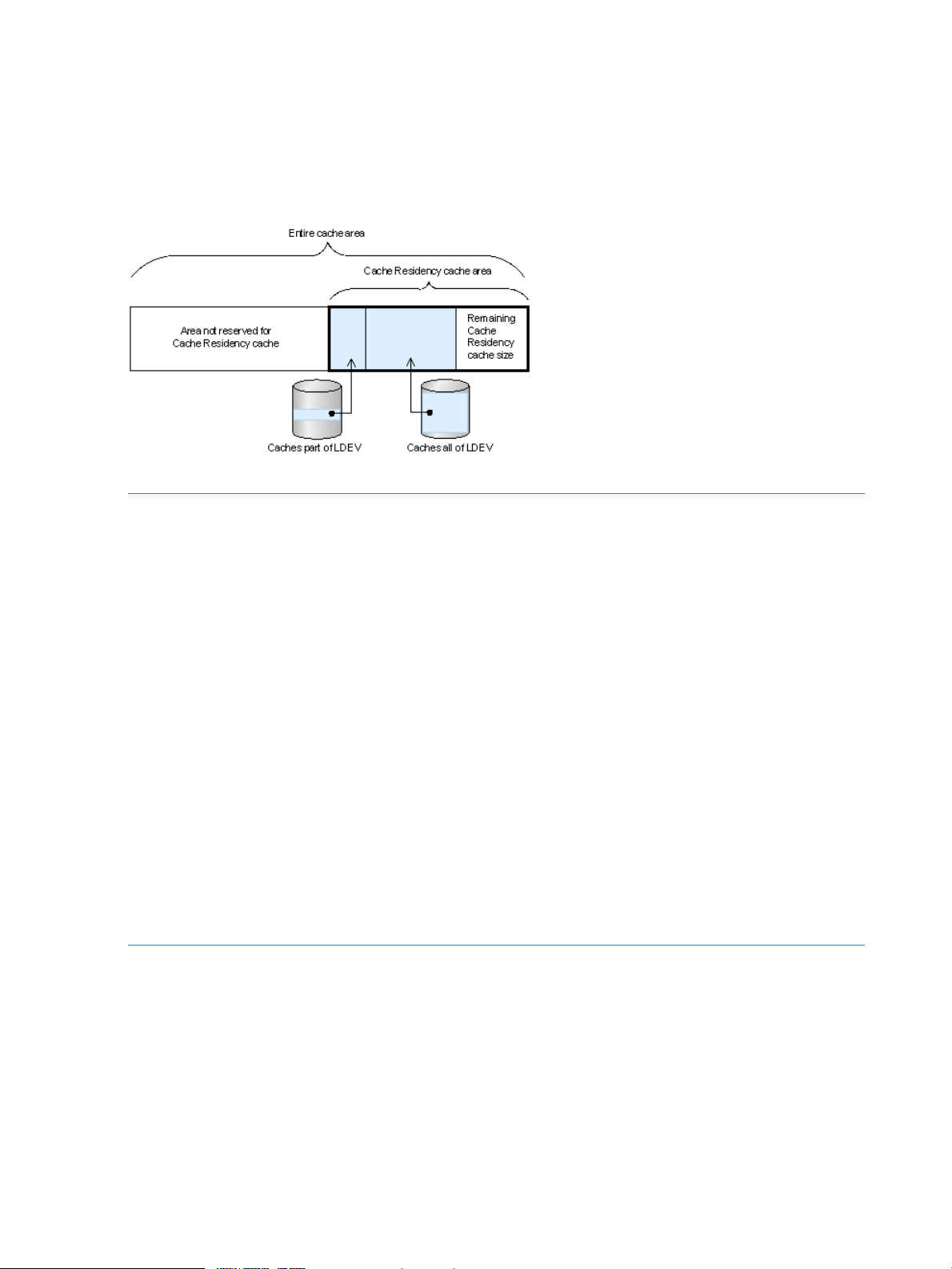
Figure 1 Cache Residency cache area
NOTE:
• If the Cache Residency cache area is accessed for I/O before the prestaging operation is
complete, the data may not be available in cache at the first I/O access.
• To prevent slow response times for host I/Os, the storage system may interrupt the prestaging
operation when the cache load is heavy.
• Do not use the prestaging function if you specify the Cache Residency setting on a volume
during the quick formatting operation. To use the prestaging function after the quick formatting
operation completes, first release the Cache Residency setting and then specify the setting
again with the prestaging setting enabled. For information about quick formatting, see the HP
XP P9000 Provisioning for Open Systems User Guide or HP XP P9000 Provisioning for
Mainframe Systems User Guide.
• When external volumes are configured in the storage system, you need to disconnect the
external storage system before powering off the storage system. If you power off the storage
system without performing the disconnect external storage system operation and then turn on
the power supply again, the prestaging process is aborted. If the prestaging process is aborted,
you need to perform the prestaging operation again.
The prestaging process is aborted if a volume is created, deleted, or restored during the
prestaging operation. If the prestaging process is aborted, you need to perform the prestaging
operation again after the create, delete, or restore volume operation is complete.
Priority mode (read data only)
In priority mode the Cache Residency extents are used to hold read data for specific extents on
volumes. Write data is write duplexed in cache other than Cache Residency cache, and the data
is destaged to the drives when disk utilization is low.
The required total cache capacity for priority mode (normal mode) is:
standard cache + Cache Residency cache + additional cache
The next table specifies the standard cache capacity requirements for priority mode operations.
Meeting these requirements is important for preventing performance degradation. For more
information about calculating cache size for priority mode, see “Estimating cache size” (page 69).
10 Performance overview
Page 11

Table 1 Cache capacity requirements for CR priority mode
capacity is 128 GB or less
capacity exceeds 128 GB
1 GB = 1,073,741,824 bytes
Bind mode (read and write data)
In bind mode the Cache Residency extents are used to hold read and write data for specific extents
on volumes. Data written to the Cache Residency bind area is not destaged to the drives. To ensure
data integrity, write data is duplexed in the Cache Residency cache area, which consumes a
significant amount of the Cache Residency cache.
Bind mode provides the following advantages over priority mode:
• The accessibility of read data is the same as Cache Residency priority mode.
• Write operations do not have to wait for available cache segments.
• There is no back-end contention caused by destaging data.
The required total cache capacity for bind mode is:
standard cache + Cache Residency cache
Cache Residency bind data that has write attributes is normally not destaged. However, the data
is destaged to disk in the following cases:
Standard cache capacitySettings of priority mode
16 GBSpecified number of cache areas is 8,192 or less and the specified
32 GBSpecified number of cache areas exceeds 8,192 or the specified
• During cache blockage that is caused by certain maintenance operations (for example, cache
upgrades) or by cache failure.
• When the storage system is powered off.
• When the volume is deleted from Cache Residency bind mode.
The next table specifies the cache requirements for bind mode operations. Meeting these
requirements is important for preventing performance degradation. For more information about
calculating cache size for bind mode, see “Estimating cache size” (page 69).
Table 2 Bind mode cache requirements
System Type
Open systems
Type
RAID 5 (3390) or RAID
6
RAID 1, or external
volumes
Capacity SpecificationsRAID Level or Volume
Slot capacity: 264 KB
Cache segment capacity: 16.5 KB
Cache segments needed per slot: 48
(slot capacity / cache segment
capacity)
Slot capacity: 264 KB
Cache segment capacity: 16.5 KB
Cache segments needed per slot: 32
(slot capacity / cache segment
capacity)
Cache Residency Cache
Requirement
3 times the space required for
user data: 1 slot = 3 × 264
KB = 792 KB = 48 cache
segments
2 times the space required for
user data: 1 slot = 2 × 264
KB = 528 KB = 32 cache
segments
Mainframe (for
example, 3390-3,
3390-9)
RAID 5 mainframe or
RAID 6
Slot capacity: 66 KB
Cache segment capacity: 16.5 KB
3 times the space required for
user data: 1 slot = 3 × 66 KB
Cache Residency overview 11
Page 12

Table 2 Bind mode cache requirements (continued)
System Type
Type
RAID 1 mainframe, or
external volumes
Capacity SpecificationsRAID Level or Volume
Cache segments needed per slot: 12
(slot capacity / cache segment
capacity)
Note: Even though a mainframe track
is 56 KB, because cache is divided
into 16.5 KB segments, it requires 4
segments.
Slot capacity: 66 KB
Cache segment capacity: 16.5 KB
Cache segments needed per slot: 8
(slot capacity / cache segment
capacity)
Cache Residency Cache
Requirement
= 198 KB = 12 cache
segments
2 times the space required for
user data: 1 slot = 2 × 66 KB
= 132 KB = 8 cache
segments
12 Performance overview
Page 13
2 About performance monitoring
This topic presents an overview of Performance Monitor and Cache Residency.
Monitoring storage system resources
Performance Monitor enables you to monitor your storage system and collect detailed usage and
performance statistics. If there is a decrease in storage system performance (for example, delayed
host response times), Performance Monitor can help you detect the cause of the problem and
resolve it.
Performance Control uses the data collected by Performance Monitor to identify and resolve
bottlenecks of activity on the ports.
Placing data in cache
Cache Residency enables you to place specific data into user-defined Cache Residency cache
areas, also called cache extents, so that the data is available to hosts at front-end data transfer
speeds. This is called prestaging data in cache.
Prestaging specific data
Cache Residency supports prestaging of data in which specific data is placed into the Cache
Residency cache before it is accessed by the host. When prestaging is used, the host locates the
prestaged data in the Cache Residency cache during the first access, thereby improving
performance.
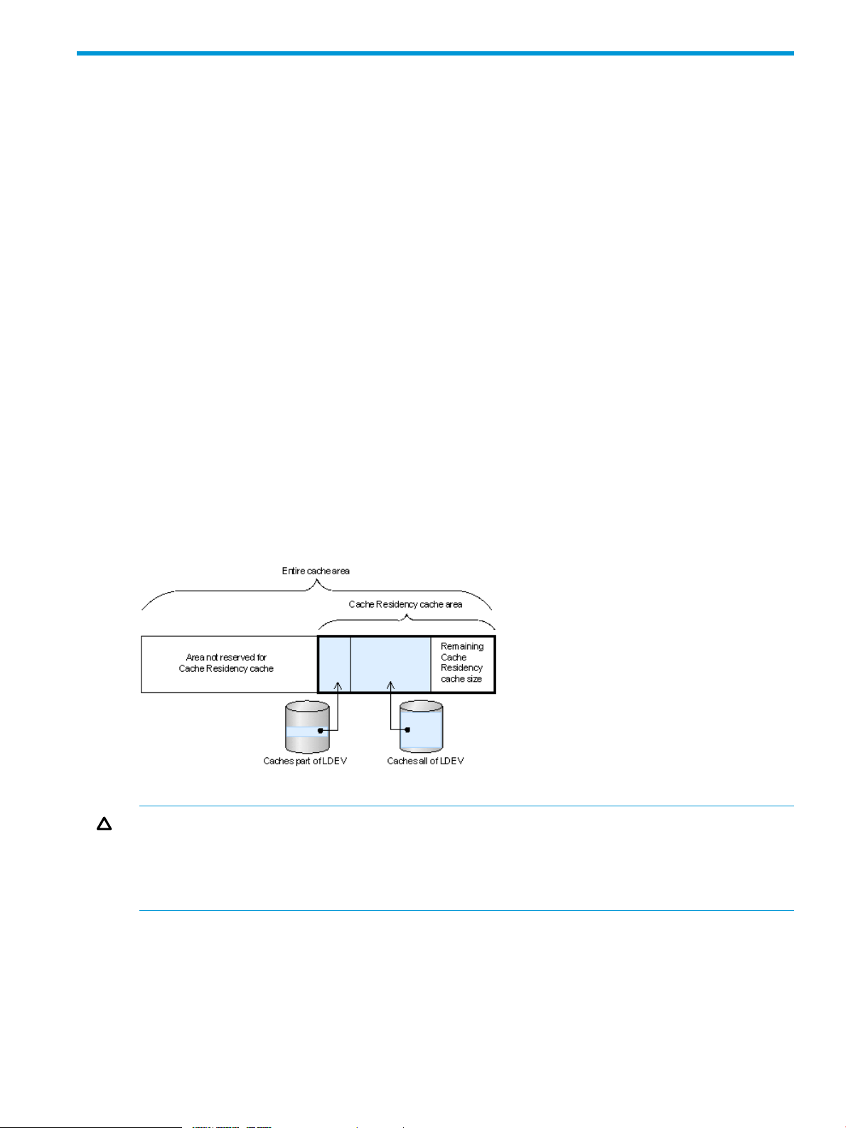
Figure 2 Cache Residency cache area
CAUTION: Total storage system cache capacity must be increased when using Cache Residency
to avoid data access performance degradation for non-cache-resident data. Cache Residency is
available only on HP XP P9500 storage systems configured with at least 512 MB of cache. The
HP representative configures the maximum allowable Cache Residency area when the cache is
installed.
Both priority mode and bind mode permit prestaging. Prestaging occurs under any of the following
circumstances:
• When prestaging is performed from the SVP or from Remote Web Console.
• When the power is turned on.
• When cache maintenance is performed.
Monitoring storage system resources 13
Page 14

NOTE:
• If you access the Cache Residency area for input and output before the prestaging operation
is performed from the SVP or Remote Web Console, the host may not be able to find data in
the cache at the first I/O access after Cache Residency is configured.
• To prevent the slow response time of the host I/O, the prestaging operation may be interrupted
when the cache load is heavy.
• If you specify the Cache Residency setting on the volume during the quick formatting, do not
use the prestaging function. If you want to use the prestaging function after the quick formatting
processing completes, first release the setting and then specify the Cache Residency setting
again, with the prestaging setting enabled. For information about the quick formatting, see
HP XP P9000 Provisioning for Open Systems User Guide or HP XP P9000 Provisioning for
Mainframe Systems User Guide.
• When external volumes are set in the storage system, execute the disconnect external storage
system operation to the external storage system before turning off the power supply of the
storage system. If you turn off the power supply of the storage system without executing the
disconnect external storage system operation to the external storage system and then turn on
the power supply again, the prestaging processing is aborted. If the prestaging processing is
aborted, perform the prestaging operation from SVP or Remote Web Console.
The prestaging processing is aborted if a volume is created, deleted, or restored during the
prestaging operation. If the prestaging processing is aborted, perform the prestaging operation
from SVP or Remote Web Console after finishing a volume create, delete, or restore volume
operation.
Priority mode
In priority mode the Cache Residency extents are used to hold read data for specific extents on
volumes. Write data is write duplexed in cache other than that of Cache Residency, and the data
is destaged to the disk drive when disk utilization is low.
In priority mode (normal mode), the total capacity of cache required is:
standard cache + Cache Residency cache + additional cache
The following table specifies the standard cache capacity requirements for Cache Residency priority
mode operations. Meeting these requirements is important for preventing performance degradation.
For more information about calculating cache size for priority mode, see “Estimating cache size”
(page 69).
Table 3 Cache capacity requirements for CR priority mode
and the specified capacity is 128 GB or less
or the specified capacity exceeds 128 GB
1 GB = 1,073,741,824 bytes
Bind mode
Standard cache capacitySettings of priority mode
16 GBSpecified number of cache areas is 8,192 or less
32 GBSpecified number of cache areas exceeds 8,192
Cache Residency uses extents to hold read and write data for specific extents on volumes. Data
written to the Cache Residency bind area is not destaged to the disk. To ensure data integrity,
write data is duplexed in the Cache Residency area, which consumes a significant amount of the
Cache Residency cache.
14 About performance monitoring
Page 15

Bind mode has the following advantages:
• The accessibility of read data is the same as Cache Residency priority mode.
• Write operations do not have to wait for available cache segments.
• There is no back-end contention caused by destaging data.
In Bind Mode, the total capacity of cache required is:
standard cache + Cache Residency cache
For more information about calculating case size for bind mode, see “Estimating cache size”
(page 69).
The next table specifies the cache requirements for bind mode operations:
Table 4 Bind mode cache requirements
System Type
OPEN Systems
Mainframe (for example,
3390-3, 3390-9)
Type
RAID 5 (3390) or RAID
6
RAID 1, or external
volumes
RAID 5 mainframe or
RAID 6
Capacity SpecificationsRAID Level or Volume
Slot capacity: 264 KB
Cache segment capacity: 16.5
KB
Cache segments needed per
slot: 48 (slot capacity / cache
segment capacity)
Slot capacity: 264 KB
Cache segment capacity: 16.5
KB
Cache segments needed per
slot: 32 (slot capacity / cache
segment capacity)
Slot capacity: 66 KB
Cache segment capacity: 16.5
KB
Cache segments needed per
slot: 12 (slot capacity / cache
segment capacity)
Note: Even though a mainframe
track is 56 KB, because cache
is divided into 16.5 KB
segments, it requires 4
segments.
Cache Residency Cache
Requirement
3 times the space required for
user data: 1 slot = 3 × 264
KB = 792 KB = 48 cache
segments
2 times the space required for
user data: 1 slot = 2 × 264
KB = 528 KB = 32 cache
segments
3 times the space required for
user data: 1 slot = 3 × 66 KB
= 198 KB = 12 cache
segments
RAID 1 mainframe, or
external volumes
Slot capacity: 66 KB
Cache segment capacity: 16.5
KB
Cache segments needed per
slot: 8 (slot capacity / cache
segment capacity)
2 times the space required for
user data: 1 slot = 2 × 66 KB
= 132 KB = 8 cache
segments
Cache Residency bind data that has write attributes is normally not destaged. However, the data
is destaged in the following cases:
• During cache blockage that is caused by certain maintenance operations (for example, cache
upgrades) or by cache failure.
• If the storage system is powered off.
• If the volume is deleted from Cache Residency bind mode.
Bind mode 15
Page 16

Changing the mode without cache extension requires reconfiguring Cache Residency (for example,
release the data from cache, and then place the data back in cache with the desired mode).
16 About performance monitoring
Page 17

3 Interoperability of Performance Monitor and other products
This chapter describes the interoperability of Performance Monitor and other products.
Cautions and restrictions for monitoring
• Storage system maintenance
If the storage system is undergoing the following maintenance operations during monitoring,
the monitoring data might contain extremely large values.
◦ Adding, replacing, or removing cache memory.
◦ Adding, replacing, or removing data drives.
◦ Changing the storage system configuration.
◦ Replacing the microprogram.
◦ Formatting or quick formatting logical devices
◦ Adding on, replacing, or removing MP blades
• Storage system power-off
If the storage system is powered off during monitoring, monitoring stops while the storage
system is powered off. When the storage system is powered up again, monitoring continues.
However, Performance Monitor cannot display information about the period while the storage
system is powered off. Therefore, the monitoring data immediately after powering on again
might contain extremely large values.
• Microprogram replacement
After the microprogram is replaced, monitoring data is not stored until the service engineer
releases the SVP from Modify mode. While the SVP is in Modify mode, inaccurate data is
displayed.
• Changing the SVP time setting
If the SVP time setting is changed while the monitoring switch is enabled, the following
monitoring errors can occur:
◦ Invalid monitoring data appears.
◦ No monitoring data is collected.
To change the SVP time setting, first disable the monitoring switch, change the SVP time setting,
and then re-enable the monitoring switch. After that, obtain the monitoring data. For details
about the monitoring switch, see “Starting monitoring” (page 28).
• WWN monitoring
You must configure some settings before the traffic between host bus adapters and storage
system ports can be monitored. For details, see “Adding new WWNs to monitor” (page 23),
“Adding WWNs to ports” (page 23), and “Connecting WWNs to ports” (page 24).
Cautions and restrictions for monitoring 17
Page 18

Cautions and restrictions for usage statistics
• Usage statistics for the last three months (93 days) are displayed in long-range monitoring,
and usage statistics for up to the last 15 days are displayed in short-range monitoring. Usage
statistics outside of these ranges are deleted from the storage system.
• In the short range, monitoring results are retained for the last 8 hours to 15 days depending
on the specified gathering interval. If the retention period has passed since a monitoring result
was obtained, the previous result has been deleted from the storage system and cannot be
displayed.
• When the monitoring switch is set to disabled, no monitoring data is collected. This applies
to both long-range and short-range data.
• For short-range monitoring, if the host I/O workload is high, the storage system gives higher
priority to I/O processing than to monitoring. If this occurs, some monitoring data might be
missing. If monitoring data is missing frequently, use the Edit Time Range option to lengthen
the collection interval. For details, see “Starting monitoring” (page 28).
• The monitoring data (short-range and long-range) may have a margin of error.
• If the SVP is overloaded, the system might require more time than the gathering interval allows
to update the display of monitoring data. If this occurs, some portion of monitoring data is
not displayed. For example, suppose that the gathering interval is 1 minute. In this case, if
the display in the Performance Management window is updated at 9:00 and the next update
occurs at 9:02, the window (including the graph) does not display the monitoring result for
the period of 9:00 to 9:01. This situation can occur when the following maintenance operations
are performed:
◦ Adding, replacing, or removing cache memory.
◦ Adding, replacing, or removing data drives.
◦ Changing the storage system configuration.
◦ Replacing the microprogram.
• Pool-VOLs of Fast Snap, Snapshot, Thin Provisioning, and Thin Provisioning Z are not monitored.
NOTE: When you run the RAID Manager horctakeover or pairresync-swaps command for a Cnt
Ac-J pair or the BCM YKRESYNC REVERSE command for a Cnt Ac-J Z pair, the primary and
secondary volumes are swapped. You can collect the before-swapped information immediately
after you run any of the commands. Incorrect monitoring data will be generated for a short time
but will be corrected automatically when the monitoring data gets updated. The incorrect data will
also be generated when the volume used for a secondary volume is used as a primary volume
after a Cnt Ac-J or Cnt Ac-J Z pair is deleted.
Using Performance Control
• Starting Performance Control. Ensure that the Time Range in the Monitor Performance window
is not set to Use Real Time. You cannot start Performance Control in real-time mode.
• I/O rates and transfer rates. Performance Control runs based on I/O rates and transfer rates
measured by Performance Monitor. Performance Monitor measures I/O rates and transfer
rates every second, and calculates the average I/O rate and the average transfer rate for
every gathering interval (specified between 1 and 15 minutes) regularly.
Suppose that 1 minute is specified as the gathering interval and the I/O rate at the port 1-A
changes as illustrated in Graph 1. When you use Performance Monitor to display the I/O
rate graph for 1A, the line in the graph indicates changes in the average I/O rate calculated
every minute (refer to Graph 2). If you select the Detail check box in the Performance Monitor
18 Interoperability of Performance Monitor and other products
Page 19
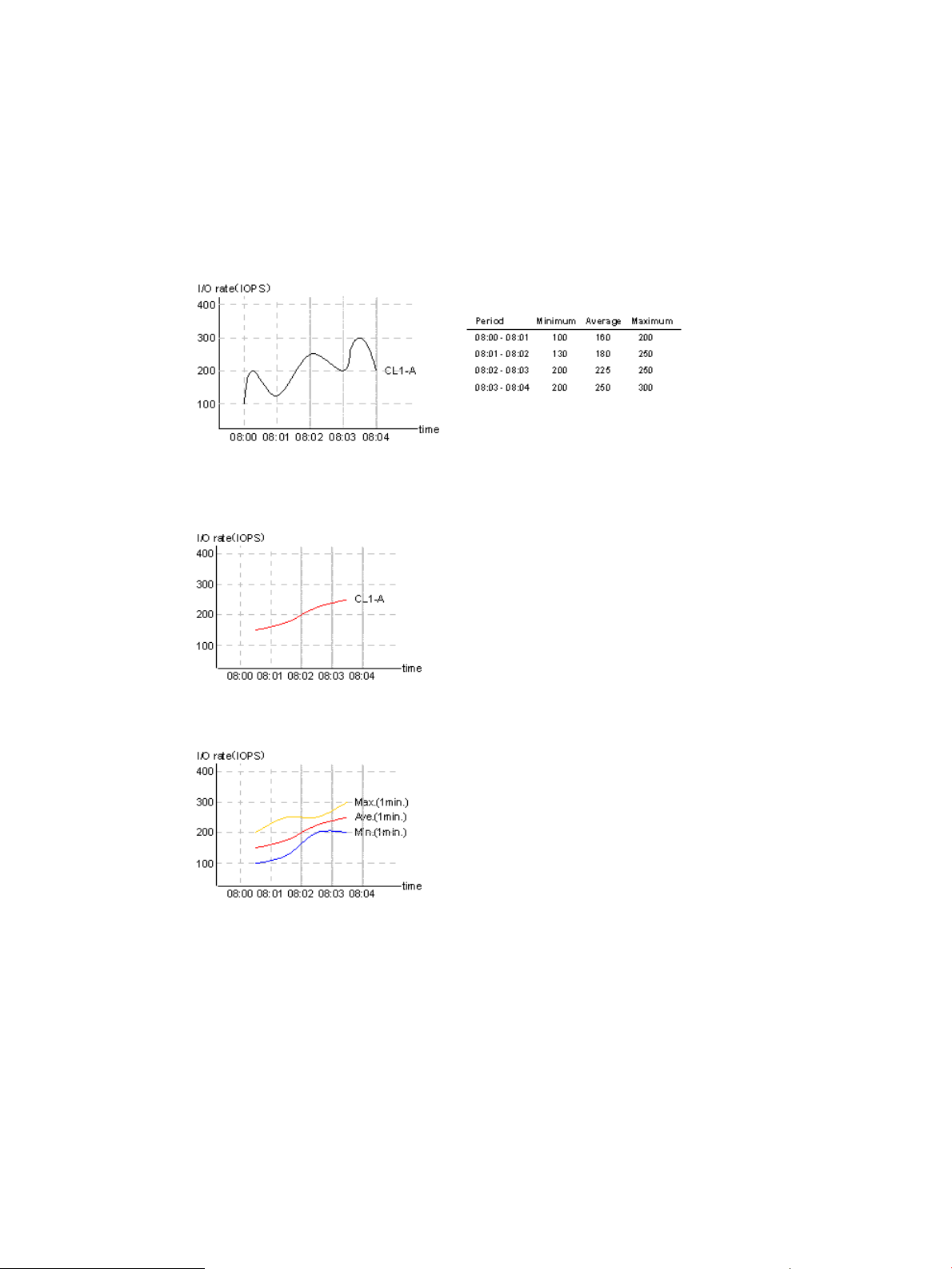
windows, the graph displays changes in the maximum, average, and minimum I/O rates in
one minute.
Performance Control applies upper limits and thresholds to the average I/O rate or the average
transfer rate calculated every gathering interval. For example, in the following figures in which
the gathering interval is 1 minute, if you set an upper limit of 150 I/Os to the port 1A, the
highest data point in the line CL1-A in Graph 2 and the line Ave.(1 min) in Graph 3 is
somewhere around 150 I/Os. It is possible that the lines Max (1 min.) and Min (1 min.) in
Graph 3 might exceed the upper limit.
Figure 3 Graph 1: actual I/O rate (measured every second)
Figure 4 Graph 2: I/O rate displayed in Performance Monitor (the Detail check box is not
selected)
Figure 5 Graph 3: I/O rate displayed in Performance Monitor (the Detail check box is selected)
Using Performance Control 19
Page 20

NOTE:
• Continuous Access Synchronous: Performance Control monitors write I/O requests issued from
initiator ports of your storage system.
• When the remote copy functions: (Continuous Access Synchronous, Continuous Access
Synchronous Z, Continuous Access Journal, and Continuous Access Journal Z) are used in
your environment, Performance Control monitors write I/O requests issued from initiator ports
of your storage system.
If you give a priority attribute to the RCU target port, all I/Os received on the port will be
controlled as the threshold control and its performance data will be added to the total number
of I/Os (or the transfer rate) of all prioritized ports. I/Os on the port will not be limited.
If you give a non priority attribute to the RCU target port, I/O requests from the initiator port
will not be controlled as threshold control and I/Os on the port will not be limited. On the
other hand, I/O requests from a host will be controlled as the upper limit control and I/Os
on the port will be limited.
• Statistics of Initiator/External ports: The initiator ports and external ports of your storage system
are not controlled by Performance Control. Although you can set Prioritize or Non-Prioritize
to initiator ports and external ports by using Performance Control, the initiator ports and the
external ports become the prioritized ports that are not under threshold control, regardless of
whether the setting of the ports are Prioritize or Non-Prioritize. If the port attributes are changed
from Initiator/External into Target/RCU Target, the settings by Performance Control take effect
instantly and the ports are subject to threshold or upper limit control.
The statistics of the Monitor Performance window are the sum of the statistics on Target/RCU
Target ports that are controlled by Performance Control. The statistics do not include the
statistics of Initiator/External ports. Because the statistics of Initiator/External ports and
Target/RCU Target ports are based on different calculation methods, it is impossible to sum
up the statistics of Initiator/External ports and Target/RCU Target ports.
• Settings of Performance Control main window: The Performance Control main window has
two tabs: the Port tab and the WWN tab. The settings on only one tab at a time can be applied
to the storage system. If you make settings on both tabs, the settings cannot be applied at the
same time. When you select Apply, the settings on the last tab on which you made settings
are applied, and the settings on the other tab are discarded.
NOTE:
• Settings for Performance Control from RAID Manager: You cannot operate Performance Control
from RAID Manager and Remote Web Console simultaneously.If you change some settings
for Performance Control from RAID Manager, you cannot change those settings from Remote
Web Console. If you do, some settings might not appear. Before you change features that
use Performance Control, delete all Performance Control settings from the currently used
features.
WWN monitoring data
You must configure some settings before you start monitoring traffic between host bus adapters
and storage system ports. For details, see topics between “Viewing the WWNs that are being
monitored” (page 23) and “Deleting unused WWNs from monitoring targets” (page 25).
Microprogram replacement
After the microprogram is replaced, the monitoring data is not stored until a service engineer
releases the SVP from Modify mode. While the SVP is in Modify mode, inaccurate data is displayed.
20 Interoperability of Performance Monitor and other products
Page 21
Changing the time setting of SVP
If the monitoring switch function is performed, do not change the time setting of the SVP. If the time
setting is changed, the following problems can happen:
• Invalid monitoring data appears.
• No monitoring data is collected.
If the time setting of the SVP is changed, turn off the monitoring switch, and then turn on the switch.
After that, obtain the monitoring data. For details about the monitoring switch, see “Starting
monitoring” (page 28).
Using Performance Control
• When starting Performance Control. Ensure that the Time Range in the Monitor Performance
window is not set to Use Real Time. You cannot start Performance Control in real-time mode.
• Performance Control runs based on I/O rates and transfer rates measured by Performance
Monitor. Performance Monitor measures I/O rates and transfer rates every second, and
calculates the average I/O rate and the average transfer rate for each gathering interval
(specified between 1 and 15 minutes).
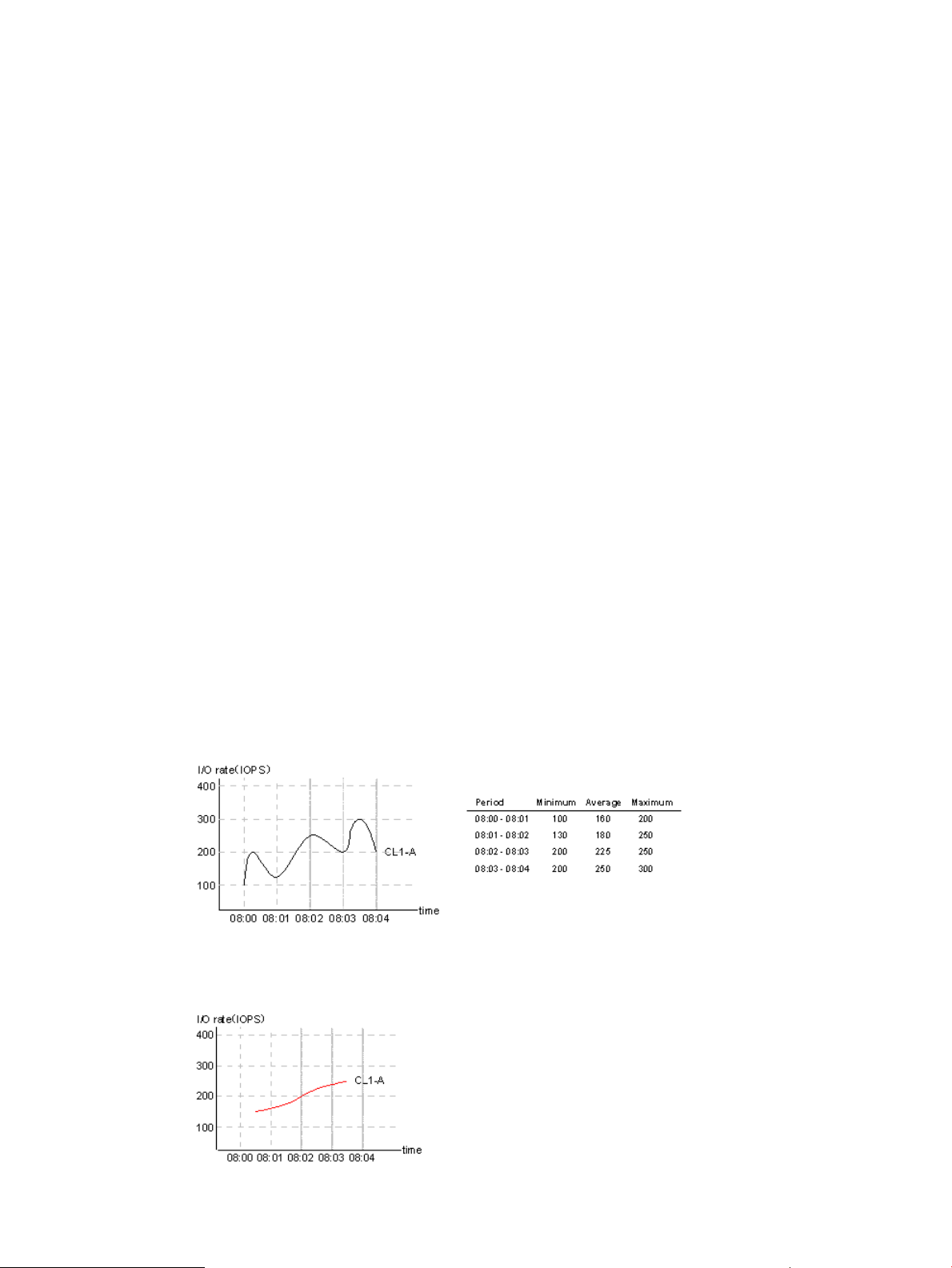
Suppose that 1 minute is specified as the gathering interval and the I/O rate at the port 1-A
changes as illustrated in Graph 1. When you use Performance Monitor to display the I/O
rate graph for 1A, the line in the graph indicates changes in the average I/O rate calculated
every minute (refer to Graph 2). If you select the Detail check box in the Performance Monitor
windows, the graph displays changes in the maximum, average, and minimum I/O rates in
one minute.
Performance Control applies upper limits and thresholds to the average I/O rate or the average
transfer rate calculated every gathering interval. For example, in the following figures in which
the gathering interval is 1 minute, if you set an upper limit of 150 I/Os to the port 1A, the
highest data point in the line CL1-A in Graph 2 and the line Ave.(1 min) in Graph 3 is
somewhere around 150 I/Os. It is possible that the lines Max (1 min.) and Min (1 min.) in
Graph 3 might exceed the upper limit.
Figure 6 Graph 1: actual I/O rate (measured every second)
Figure 7 Graph 2: I/O rate displayed in Performance Monitor (the Detail check box is not
selected)
Changing the time setting of SVP 21
Page 22
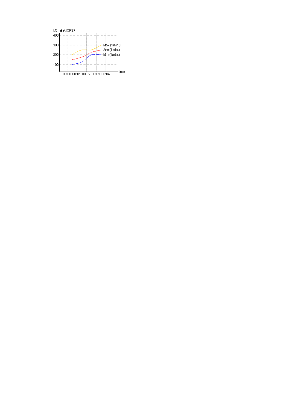
Figure 8 Graph 3: I/O rate displayed in Performance Monitor (the Detail check box is selected)
NOTE:
• Continuous Access Synchronous: Performance Control monitors write I/O requests issued from
initiator ports of your storage system.
• When the remote copy functions: (Continuous Access Synchronous, Continuous Access
Synchronous Z, Continuous Access Journal, and Continuous Access Journal Z) are used in
your environment, Performance Control monitors write I/O requests issued from initiator ports
of your storage system.
If you give a priority attribute to the RCU target port, all I/Os received on the port will be
controlled as the threshold control and its performance data will be added to the total number
of I/Os (or the transfer rate) of all prioritized ports. I/Os on the port will not be limited.
If you give a non priority attribute to the RCU target port, I/O requests from the initiator port
will not be controlled as threshold control and I/Os on the port will not be limited. On the
other hand, I/O requests from a host will be controlled as the upper limit control and I/Os
on the port will be limited.
• Statistics of Initiator/External ports: The initiator ports and external ports of your storage system
are not controlled by Performance Control. Although you can set Prioritize or Non-Prioritize
to initiator ports and external ports by using Performance Control, the initiator ports and the
external ports become the prioritized ports that are not under threshold control, regardless of
whether the setting of the ports are Prioritize or Non-Prioritize. If the port attributes are changed
from Initiator/External into Target/RCU Target, the settings by Performance Control take effect
instantly and the ports are subject to threshold or upper limit control.
The statistics of the Monitor Performance window are sum total of statistics on Target/RCU
Target ports that are controlled by Performance Control. The statistics does not include the
statistics of Initiator/External ports. Because the statistics of Initiator/External ports and
Target/RCU Target ports are based on different calculation methods, it is impossible to sum
up the statistics of Initiator/External ports and Target/RCU Target ports.
• Settings of Performance Control main window: The settings in the Port tab or the WWN tab
are valid as the current settings in the Performance Control main window. All port settings in
the invalid tab are invalid regardless of the resources that are assigned to you. You can confirm
the current status in Current Control Status which appears in the upper right of the Performance
Control main window.
NOTE:
• Settings for Performance Control from RAID Manager: You cannot operate Performance Control
from RAID Manager and Remote Web Console simultaneously.If you change some settings
for Performance Control from RAID Manager, you cannot change those settings from Remote
Web Console. If you do, some settings might not appear. Before you change features that
use Performance Control, delete all Performance Control settings from the currently used
features.
22 Interoperability of Performance Monitor and other products
Page 23

4 Monitoring WWNs
This topic describes how to set up WWNs to be monitored.
Viewing the WWNs that are being monitored
To view the WWNs that are being monitored:
1. Display the Remote Web Console main window.
2. Select Performance Monitor in Explorer, and select Performance Monitor in the tree.
The Performance Monitor window opens.
3. Select the Monitored WWNs tab to see the list of WWNs that are currently being monitored.
Adding new WWNs to monitor
To add new WWNs to monitor:
1. Display the Remote Web Console main window.
2. Select Performance Monitor in Explorer, and select Performance Monitor in the tree.
The Performance Monitor window opens.
3. Select the Monitored WWNs tab.
4. Click Edit WWN Monitor Mode.
The Edit WWN Monitor Mode window opens.
5. Select the WWNs in the Unmonitored WWNs list, and click Add.
6. Click Finish to display the Confirm window.
7. Click Apply in the Confirm window to apply the settings to the storage system.
Removing WWNs to monitor
To remove WWNs to monitor:
1. Display the Remote Web Console main window.
2. Select Performance Monitor in Explorer, and select Performance Monitor in the tree.
The Performance Monitor window opens.
3. Click the Monitored WWNs tab.
4. Click Edit WWN Monitor Mode.
The Edit WWN Monitor Mode window opens.
5. Select the WWNs in the Monitored WWNs list that you want to remove, and click Remove.
6. Click Finish to display the Confirm window.
7. Click Apply in the Confirm window.
8. When the warning message appears, click OK to close the message. The settings are applied
to the storage system.
Adding WWNs to ports
If you want to monitor WWNs that are not connected to the storage system, you can add them to
ports and set them up for monitoring with Performance Monitor.
1. Display the Remote Web Console main window.
2. Select Performance Monitor in Explorer, and select Performance Monitor in the tree.
The Performance Monitor window opens.
3. Click the Monitored WWNs tab.
Viewing the WWNs that are being monitored 23
Page 24

4. Click Add New Monitored WWNs.
The Add New Monitored WWNs window opens.
5. Specify the following information for each new WWN:
• HBA WWN (required)
Enter the 16-digit hexadecimal number.
• WWN Name (optional)
Enter the unique name to distinguish the host bus adapter from others. The WWN Name
must be less than 64 characters and must consist of alphanumeric characters and at least
one symbol.
• Port (In Available Ports)
In the Available Ports list select the port connected to the WWN. Ports connected to
mainframe hosts are not displayed, because they are not supported for Performance
Monitor.
6. Click Add. The added WWN is displayed in Selected WWNs.
7. If you need to remove a WWN from the Selected WWNs list, select the WWN and click
Remove.
8. When you are done adding new WWNs, click Finish.
9. Click Apply in the Confirm window to apply the settings to the storage system.
Editing the WWN nickname
To edit the nickname of a WWN being monitored:
1. Display the Remote Web Console main window.
2. Select Performance Monitor in Explorer, and select Performance Monitor in the tree.
The Performance Monitor window opens.
3. Click the Monitored WWNs tab to see the list of WWNs being monitored.
4. Select the WWN to edit, and click Edit WWN. You can edit only one WWN at a time. If you
select multiple WWNs, an error will occur.
The Edit WWN window opens.
5. Edit the HBA WWN and WWN Name fields as needed.
• HBA WWN
A 16-digit hexadecimal number. The value of HBA WWN must be unique in the storage
system.
• WWN Name
The nickname distinguishes the host bus adapter from others. The WWN Name must be
less than 64 digits and must consist of alphanumeric characters and at least one symbol.
6. Click Finish to display the Confirm window.
7. Click Apply in the Confirm window to apply the settings to the storage system.
Connecting WWNs to ports
To connect the WWNs to monitor to ports:
1. Display the Remote Web Console main window.
2. Select Performance Monitor in Explorer, and select Performance Monitor in the tree.
The Performance Monitor window opens.
3. Click the Monitored WWNs tab.
24 Monitoring WWNs
Page 25

4. Select the WWN to connect to the port, and click Add to Ports.
The Add to Ports window opens. If you select a WWN to connect, select one WWN in the
list. If you select multiple WWNs and click Add to Ports, an error occurs.
5. Select a port to connect in Available Ports, and then click Add. However, the ports of the
mainframe system are not displayed in the list because they are not supported for Performance
Monitor.
The added WWN and the port are specified for the Selected WWNs.
6. If necessary, select unnecessary row of a WWN and port in Selected WWNs, and then click
Remove.
WWNs are deleted.
7. Click Finish to display the Confirm window.
8. Click Apply in the Confirm window to apply the settings to the storage system.
Deleting unused WWNs from monitoring targets
To delete WWNs that are being monitored:
1. Display the Remote Web Console main window.
2. Select Performance Monitor in Explorer, and select Performance Monitor in the tree.
The Performance Monitor window opens.
3. Click the Monitored WWNs tab.
4. Click Delete Unused WWNs to display the Confirm window.
5. Click Apply in the Confirm window.
6. When the warning message appears, click OK to close the message. The settings are applied
to the storage system.
Deleting unused WWNs from monitoring targets 25
Page 26

5 Monitoring CUs
This topic describes how to set up CUs to be monitored.
Displaying CUs to monitor
To display the list of CUs to monitor:
1. Open the Remote Web Console main window.
2. Select Performance Monitor in Explorer and select Performance Monitor from the tree.
3. Open the Monitored CUs tab. View the list of CUs.
Adding or removing CUs to monitor
NOTE: When a CU is removed from monitoring, the monitor data for that CU is deleted. If you
want to save the data, export it first using the Export Tool (see “Export Tool” (page 86)), and then
remove the CU.
1. Display the Remote Web Console main window.
2. Select Performance Monitor in Explorer, and select Performance Monitor in the tree.
The Performance Monitor window opens.
3. Open the Monitored CUs tab.
4. Click Edit CU Monitor Mode.
The Edit CU Monitor Mode window opens.
5. To add CUs as monitoring target objects, select the CUs in the Unmonitored CUs list, and click
Add to move the selected CUs into the Monitored CUs list.
To add all CUs in a parity group as monitoring target objects:
1. Click Select by Parity Groups in the Unmonitored CUs area.
The Select by Parity Groups window opens. The available parity group IDs and number
of CUs are displayed.
2. Select the parity group ID from the list and click Detail.
The Parity Group Properties window opens. CUs and the number of LDEVs are displayed.
3. Confirm the properties of the parity group and click Close.
The Select by Parity Groups window opens.
4. Select the parity group to be the monitoring target in the Select by Parity Groups window,
and click OK.
The CUs in the parity group are selected in the Unmonitored CUs list.
5. Click Add to move the selected CUs into the Monitored CUs list.
6. To remove CUs as monitoring target objects, select the CUs in the Monitored CUs list, and
click Remove to move the selected CUs into the Unmonitored CUs list.
7. When you are done adding and/or deleting CUs, click Finish.
8. When the confirmation dialog box opens, click Apply.
If you are removing CUs, a warning message appears asking whether you want to continue
this operation even though monitor data will be deleted.
9. To add and remove the CUs, click OK. The new settings are registered in the system.
Confirming the status of CUs to monitor
To view the monitoring status of CUs:
26 Monitoring CUs
Page 27

1. Display the Remote Web Console main window.
2. Select Performance Monitor in Explorer, and select Performance Monitor in the tree.
The Performance Monitor window opens.
3. Open the Monitored CUs tab.
4. Click Edit CU Monitor Mode.
The Edit CU Monitor Mode window opens.
5. Click View CU Matrix in the Edit CU Monitor Mode window.
The View CU Matrix window opens. The following CUs are displayed in the Monitored CUs
window:
• Monitored CUs
• Set monitored CUs
• Release monitored CUs
6. Click Close.
The Edit CU Monitor Mode window opens.
Confirming the status of CUs to monitor 27
Page 28

6 Monitoring operation
This topic describes how to start and stop the monitoring operation.
Performing monitoring operations
This topic describes how to start or stop the monitoring operation.
• To start the monitoring operation, see “Starting monitoring” (page 28).
• To stop the monitoring operation, see “Stopping monitoring” (page 28).
Starting monitoring
To start monitoring the storage system, start Performance Monitor and open the Edit Monitoring
Switch window. If this operation is performed, the monitoring result will be deleted.
1. Display the Remote Web Console main window.
2. Select Performance Monitor in Explorer, and select Performance Monitor in the tree.
The Performance Monitor window opens.
3. Click Edit Monitoring Switch in the Performance Monitor window.
The Edit Monitoring Switch window opens.
4. Click Enable in the Monitoring Switch field.
5. Select the collecting interval in the Sample Interval.
Specify the interval to obtain usage statistics about the storage system for short range
monitoring. This option is activated when you specify Enable for Current Status. If CUs to be
monitored are 64 or less, you can specify the value between 1 and 15 minutes by minutes,
and the default setting is 1 minute. For example, if you specify 1 minute for the gathering
interval, Performance Monitor collect statistics (for example, I/O rates and transfer rates) every
one minute.
If CUs to be monitored are 65 or more, the gathering interval can be specified to the value
5, 10 or 15 minutes (in the 5 minuted interval), and default is 5 minutes. For example, if you
specify the gathering interval to 5 minutes, Performance Monitor gathers statistics (for example,
I/O rate and transfer rate) every 5 minutes.
6. Click Finish to display the Confirm window.
7. Click Apply in the Confirm window.
A warning message appears, asking whether you continue this operation although graph
data is deleted.
8. Click OK to start monitoring.
When statistics are collected, a heavy workload is likely to be placed on servers. Therefore,
the client processing might slow down.
Stopping monitoring
To stop monitoring the storage system:
1. Display the Remote Web Console main window.
2. Select Performance Monitor in Explorer, and select Performance Monitor in the tree.
The Performance Monitor window opens.
3. Click Edit Monitoring Switch in the Performance Monitor window.
The Edit Monitoring Switch window opens.
28 Monitoring operation
Page 29

4. Click Disable in the Monitoring Switch field.
The Sample Interval list is grayed out and becomes ineffective.
5. Click Finish to display the Confirm window.
6. Click Apply in the Confirm window to stop monitoring.
Stopping monitoring 29
Page 30

7 Setting statistical storage ranges
This topic describes setting statistical storage ranges.
About statistical storage ranges
Performance Monitor collects and stores statistics for two time periods (ranges): short range and
long range. The difference between the two ranges and the statistics they target are as follows:
• Short range
If the number of CUs to be monitored is 64 or less, statistics are collected at a user-specified
interval between 1 and 15 minutes, and stored between 1 and 15 days.
If the number of CUs to be monitored is 65 or more, statistics are collected at a user-specified
intervals of 5, 10, or 15 minutes, and stored for 8 hours, 16 hours, or 1 day, respectively.
• Long range
Statistics are collected at fixed 15-minute (0, 15, 30, and 45 minutes of every hour), and
stored for 93 days (for example, 3 months).
Usage statistics about storage system resources are collected and stored in long range, in
parallel with in short range. However, some of usage statistics about resources cannot be
collected in long range.
Viewing statistics
Use the Monitor Performance window to view statistics within short and long storage ranges. All
statistics, except some information related to Auto LUN V2, can be viewed in short range (for the
storing period corresponding to the collecting interval setting). In addition, usage statistics about
storage system resources can be viewed in both short range and long range because they are
monitored in both ranges. When viewing usage statistics about resources, you can specify the
range to view and which part of the storing period to depict on lists and graphics.
Setting the storing period of statistics
To set the storing period of statistics:
1. Display the Remote Web Console main window.
2. Select Performance Monitor in Explorer, and select Performance Monitor in the tree.
The Performance Monitor window opens.
3. Click Monitor Performance in the Performance Monitor window.
The Monitor Performance window opens.
4. Select Long-Range or Short-Range in the Data Range as the periods (ranges) for collecting
and storing statistics.
30 Setting statistical storage ranges
Page 31

5. Select Set Range or Use Real Time in the Time Range as the periods (ranges) for displaying
statistics.
If Long-Range is selected, you can specify only Set Range. If Short-Range is selected, you can
select Set Range or Use Real Time.
Performance Monitor saves the statistics obtained up to 1440 times in SVP. Therefore, you
can estimate the storing period of statistics with “gathering interval multiplied by 1440.” For
example, if you specify one minute for the gathering interval, the statistics for one day can be
stored at the maximum from the following formula:
1 minute x 1440 = 1440 minutes = 24 hours = 1 day
This storing period is the range of display in the Monitor Performance windows. When you
specify one minute for the gathering interval like the example above, Performance Monitor
can display the statistics for one day (for example, 24 hours) in the list and graph at the
maximum. Also, when you specify 15 minutes for the gathering interval, Performance Monitor
can display the statistics for 15 days in the list and graph at the maximum.
Setting the storing period of statistics 31
Page 32

8 Working with graphs
This topic describes how to display statistical graphs.
Basic operation
Use Monitor Performance window to display graphs.
1. Display the Performance Monitor main window.
2. Select Performance Monitor in Explorer, and select Performance Monitor in the tree.
The Performance Monitor window opens.
3. Click Monitor Performance in the Performance Monitor window.
The Monitor Performance window opens.
4. Select Long-Range or Short-Range as the storing period of statistics in the Data Range field.
5. Select Set Range or Use Real Time as the displaying period of statistics in the Time Range field.
However, Use Real Time can be specified when Short-Range is selected.
Specify items to display graphs in the Performance Objects field.
6. Select items in the Object field.
Select items in the left field and then select detailed items in the right field. Detailed item
changes by the items selected in the left field.
7. Select items in the Monitor Data field.
Select items in the left field and then select detailed items in the right field.
8. Select the item to display graph in the Performance Object Selection field.
Select the object in the Available Objects field.
9. Click Add.
The added object is displayed in the Selected Objects field.
10. To delete the unnecessary object, select the object and click Remove.
11. Click Apply.
The line graph is displayed on the graph panel in the Monitor window.
• Graphs appear on the left side and notes appear on the right of panels.
• You can change the size of the panel by clicking the icon in the upper right of the panel.
• You can view up to 8 lines in one panel.
• You can view up to 16 graphs across a total of four panels.
• In the graph panel, the unit of scale on vertical axis can be changed.
By using the list on the upper left of the graph panel, adjust the scale to display the
maximum value of the graph. If the graph is too big, the display may not be able to
displaying properly. For example, the line of the graph is too thick, or the graph panel
is painted out in the color of the graph.
• If you locate the mouse cursor to each point of the graph, a detailed value is displayed
with the tool tip.
• When you click the explanatory note on the right of the graph panel, you can display or
hide points on the graph panel. However, If the graph is displayed only the one point
on X axis, the graph is always displayed. Therefore you cannot switch the display of the
point to non-display by clicking the explanatory note.
• If Time Range is set to Use Real Time and the MP blades are displayed in explanatory
notes on the right in the graph panel, the MP blade names are displayed as text links. If
32 Working with graphs
Page 33

you click the text link, the resources assigned to an MP blade of top 20 in usage rates
are displayed on the detailed window.
12. To close the graph, click Delete Graph.
Objects that can be displayed in graphs
Set items to display graph in the Performance Objects field of the Monitor Performance window.
The outline of target objects and monitoring data that can be displayed in graphs is shown in the
following table. The monitoring data shows the average value of sampling interval. The sampling
intervals are 1 to 15 minutes and 15 minutes for Short Range and Long Range, respectively, that
can be set in the Edit Monitoring Switch window.
Monitoring dataMonitoring target object
Usage rates of MPs (%).Controller
Usage rates of DRR (%).
Usage rates of cache (%).Cache
Write pending rates (%).
Usage rates of access path between CHA and ESW (%).Access Path
Usage rates of access path between DKA and ESW (%).
Usage rates of access path between MP Blade and ESW (%).
Usage rates of access path between cache and ESW (%).
Throughput (IOPS).Port
Data transfer (MB/s).
Response time (ms).
Throughput of WWN (IOPS).WWN
Data transfer of WWN (MB/s).
Response time of WWN (ms).
Throughput of port (IOPS).
Data transfer of port (MB/s).
Response time of port (ms).
Total throughput (IOPS).Logical Device
Read throughput (IOPS).
Write throughput (IOPS).
Cache hit (%).
Data transfer (MB/s).
Response time (ms).
Back transfer (count/sec).
Drive usage rate (%). *
Drive access rate (%). *
Usage rates of Business Copy (%). *
Total throughput (IOPS).Parity Group
Read throughput (IOPS).
1
1
Objects that can be displayed in graphs 33
1
Page 34

Monitoring dataMonitoring target object
Write throughput (IOPS).
Cache hit (%).
Data transfer (MB/s).
Response time (ms).
Back transfer (count/sec).
Drive usage rate (%). *
Total throughput (IOPS).LUN
Read throughput (IOPS).
Write throughput (IOPS).
Cache hit (%).
Data transfer (MB/s).
Response time (ms).
Back transfer (count/sec).
Data transfer of logical devices (MB/s).External Storage
Response time of logical devices (ms).
1
1. Only information on internal volumes is displayed. Information on external volumes and FICON DM volumes is not
displayed.
2. The same value is output to all LUNs mapped to the LDEV.
Usage rates of MPs
Function
The usage rate of the MP shows the usage rate of an MP assigned to a logical device. If a usage
rate of an MP is high, I/Os concentrate to an MP. Examine the distribution of I/Os to other MP
blades.
Storing period
Short-Range or Long-Range can be specified.
Selection of monitoring objects
Select monitoring objects in Performance Objects field. The combination of items is shown as
follows.
Data transfer of parity groups (MB/s).
Response time of parity groups (ms).
Item on left side of Object
field
34 Working with graphs
Item on right side of Object
field
Item on left side of Monitor
Data field
Item on right side of Monitor
Data field
NoneUsage Rate (%)MPController
Page 35

Usage rate of a data recovery and reconstruction processor
Function
A data recovery and reconstruction processor (DRR) is a microprocessor (located on the DKAs and
channel adapters) that is used to generate parity data for RAID 5 or RAID 6 parity groups. The
DRR uses the formula "old data + new data + old parity" to generate new parity.
If the monitor data shows high DRR usage overall, this can indicate high write penalty condition.
Please consult your HP representative about high write penalty conditions.
Storing period
Short-Range or Long-Range can be specified.
Selection of monitoring objects
Select monitoring objects in Performance Objects field. The combination of items is shown as
follows.
Item on left side of Object
field
Item on right side of Object
field
Usage rate of cache memory
Function
When you display monitoring results in a short range, the window displays the usage rates about
the cache memory for the specified period of time.
Storing period
Short-Range can be specified.
Selection of monitoring objects
Select monitoring objects in Performance Objects field. The combination of items is shown as
follows.
Item on left side of Object
field
Item on right side of Object
field
Item on left side of Monitor
Data field
Item on left side of Monitor
Data field
Item on right side of Monitor
Data field
NoneUsage Rate (%)DRRController
Item on right side of Monitor
Data field
NoneUsage Rate (%)NoneCache
Write pending statistics
Function
The write pending rate indicates the ratio of write pending data to the cache memory capacity.
The Monitor Performance window displays the average and the maximum write pending rate for
the specified period of time.
Storing period
Short-Range or Long-Range can be specified.
Usage rate of a data recovery and reconstruction processor 35
Page 36

Selection of monitoring objects
Select monitoring objects in Performance Objects field. The combination of items is shown as
follows.
Item on left side of Object
field
Item on right side of Object
field
Access paths usage statistics
Function
An access path is a path through which data and commands are transferred within a storage
system.
In a storage system, channel adapters control data transfer between hosts and the cache memory.
Disk adapters control data transfer between the cache memory and hard disk drives. Data transfer
does not occur between channel adapters and disk adapters. Data is transferred via the ESW (PCI
Express Switch adapter) to the cache memory.
When hosts issue commands, the commands are transferred via channel adapters to the shared
memory (SM). The content of the shared memory is checked by disk adapters.
Performance Monitor tracks and displays the usage rate for the following access paths.
• Access paths between channel adapters and the cache switch (CHA ESW)
• Access paths between disk adapters and the cache switch (DKA ESW)
• Access paths between the cache switch and the cache memory (Cache ESW)
Item on left side of Monitor
Data field
Item on right side of Monitor
Data field
NoneWrite Pending Rate (%)NoneCache
• Access paths between the MP blade and the cache switch (MP Blade ESW)
Figure 9 Access paths
Storing period
Short-Range or Long-Range can be specified.
36 Working with graphs
Page 37

Selection of monitoring objects
Select monitoring objects in Performance Objects field. The combination of items is shown as
follows.
Item on left side of Object
field
Item on right side of Object
field
Throughput of storage system
Function
Total throughput is the sum of I/Os per second. The read throughput is I/Os to the disk per second
when the file read processing is performed. The write throughput is I/Os to the disk per second
when the file write processing is performed.
Throughput in the following modes can be displayed.
• Sequential access mode
• Random access mode
• Cache fast write (CFW) mode
• Total value in the above-mentioned mode
Item on left side of Monitor
Data field
Item on right side of Monitor
Data field
NoneUsage Rate (%)CHA ESWAccess Path
NoneUsage Rate (%)DKA ESW
NoneUsage Rate (%)MP Blade ESW
NoneUsage Rate (%)Cache ESW
Storing period
Short-Range can be specified.
Selection of monitoring objects
Select monitoring objects in Performance Objects field. The combination of items is shown as
follows.
Item on left side of Object
field
Item on right side of Object
field
Item on left side of Monitor
Data field
Item on right side of Monitor
Data field
NoneThroughput (IOPS)NonePort*
NoneThroughput (IOPS)WWNWWN*
NoneThroughput (IOPS)Port
TotalTotal Throughput (IOPS)NoneLogical Device*
Sequential
Random
CFW
TotalRead Throughput (IOPS)
Sequential
Random
CFW
Throughput of storage system 37
Page 38

Item on left side of Object
field
Item on right side of Object
field
Item on left side of Monitor
Data field
Item on right side of Monitor
Data field
TotalWrite Throughput (IOPS)
Sequential
Random
CFW
TotalTotal Throughput (IOPS)NoneParity Group*
Sequential
Random
CFW
TotalRead Throughput (IOPS)
Sequential
Random
CFW
TotalWrite Throughput (IOPS)
Sequential
* Volumes that do not accept I/O from the host, such as pool-VOLs, are not monitored.
Random
CFW
TotalTotal Throughput (IOPS)NoneLUN*
Sequential
Random
CFW
TotalRead Throughput (IOPS)
Sequential
Random
CFW
TotalWrite Throughput (IOPS)
Sequential
Random
CFW
Size of data transferred
Function
The amount of data per second transferred from the host server. The transferred data of reading
or writing process can be monitored.
Storing period
Short-Range can be specified.
38 Working with graphs
Page 39

Selection of monitoring objects
Select monitoring objects in Performance Objects field. The combination of items is shown as
follows.
Item on left side of Object
field
Item on right side of Object
field
Item on left side of Monitor
Data field
Item on right side of Monitor
Data field
NoneData Trans. (MB/s)NonePort*
NoneData Trans. (MB/s)WWNWWN*
NoneData Trans. (MB/s)Port
TotalData Trans. (MB/s)NoneLogical Device*
Read
Write
TotalData Trans. (MB/s)NoneParity Group*
Read
Write
TotalData Trans. (MB/s)NoneLUN*
Read
Write
TotalData Trans. (MB/s)Parity GroupExternal Storage*
Read
* Volumes that do not accept I/O from the host, such as pool-VOLs, are not monitored.
Response times
Function
Time (in milliseconds) for replying from an external volume group when I/O accesses are made
from the HP XP P9500 storage system to the external volume group. The average response time
in the period specified at Monitoring Term is displayed.
Items that can be monitored response times are ports, WWNs, LDEVs, parity groups, LUNs, and
external storages (parity groups and LDEVs).
Storing period
Short-Range can be specified.
Write
TotalData Trans. (MB/s)Logical Device
Read
Write
Response times 39
Page 40

Selection of monitoring objects
Select monitoring objects in Performance Objects field. The combination of items is shown as
follows.
Item on left side of Object
field
Item on right side of Object
field
Item on left side of Monitor
Data field
Item on right side of Monitor
Data field
NoneResponse Time (ms)NonePort*
NoneResponse Time (ms)WWNWWN*
NoneResponse Time (ms)Port
TotalResponse Time (ms)NoneLogical Device*
Read
Write
TotalResponse Time (ms)NoneParity Group*
Read
Write
TotalResponse Time (ms)NoneLUN*
Read
Write
TotalResponse Time (ms)Parity GroupExternal Storage*
Read
* Volumes that do not accept I/O from the host, such as pool-VOLs, are not monitored.
Cache hit rates
Function
The cash hit rate is a rate that the input or output data of the disk exists in the cache. The cash hit
rate is displayed for the sequential access mode, the random access mode, the cache fast write
(CFW) mode, and the entire these modes.
• Read hit ratio
For a read I/O, when the requested data is already in cache, the operation is classified as
a read hit. For example, if ten read requests have been made from hosts to devices in a given
time period and the read data was already on the cache memory three times out of ten, the
read hit ratio for that time period is 30 percent. A higher read hit ratio implies higher processing
speed because fewer data transfers are made between devices and the cache memory.
• Write hit ratio
For a write I/O, when the requested data is already in cache, the operation is classified as
a write hit. For example, if ten write requests were made from hosts to devices in a given time
period and the write data was already on the cache memory three cases out of ten, the write
Write
TotalResponse Time (ms)Logical Device
Read
Write
40 Working with graphs
Page 41

hit ratio for that time period is 30 percent. A higher write hit ratio implies higher processing
speed because fewer data transfers are made between devices and the cache memory.
Storing period
Short-Range can be specified.
Selection of monitoring objects
Select monitoring objects in Performance Objects field. The combination of items is shown as
follows.
Item on left side of Object
field
Item on right side of Object
field
Item on left side of Monitor
Data field
Item on right side of Monitor
Data field
Read (Total)Cache Hit (%)NoneLogical Device*
Read (Sequential)
Read (Random)
Read (CFW)
Write (Total)
Write (Sequential)
Write (Random)
Write (CFW)
Read (Total)Cache Hit (%)NoneParity Group*
Read (Sequential)
Read (Random)
Read (CFW)
Write (Total)
Write (Sequential)
* Volumes that do not accept I/O from the host, such as pool-VOLs, are not monitored.
Write (Random)
Write (CFW)
Read (Total)Cache Hit (%)NoneLUN*
Read (Sequential)
Read (Random)
Read (CFW)
Write (Total)
Write (Sequential)
Write (Random)
Write (CFW)
Cache hit rates 41
Page 42

Back-end performance
Function
The back-end transfer can be monitored. The back-end transfer is the number of data transfers
between the cache memory and the hard disk drive. The graph contains following information.
• Cache to Drive
The number of data transfers from the cache memory to hard disk drives.
• Drive to Cache Sequential
The number of data transfers from hard disk drives to the cache memory in sequential access
mode
• Drive to Cache Random
The number of data transfers from hard disk drives to the cache memory in random access
mode
Storing period
Short-Range can be specified.
Selection of monitoring objects
Select monitoring objects in Performance Objects field. The combination of items is shown as
follows.
Item on left side of Object
field
* Volumes that do not accept I/O from the host, such as pool-VOLs, are not monitored.
Item on right side of Object
field
Hard disk drive usage statistics
Item on left side of Monitor
Data field
Item on right side of Monitor
Data field
TotalBack Trans. (count/sec)NoneLogical Device*
Cache to Drive
Drive to Cache (Sequential)
Drive to Cache (Random)
TotalBack Trans. (count/sec)NoneParity Group*
Cache to Drive
Drive to Cache (Sequential)
Drive to Cache (Random)
TotalBack Trans. (count/sec)NoneLUN*
Cache to Drive
Drive to Cache (Sequential)
Drive to Cache (Random)
Function
The usage rates of the hard disk drive of each LDEV or parity group can be displayed.
42 Working with graphs
Page 43

Storing period
Short-Range can be specified.
Selection of monitoring objects
Select monitoring objects in Performance Objects field. The combination of items is shown as
follows.
Item on left side of Object
field
* Only information on internal volumes is displayed. Information about external volumes, FICON DM volumes, and
virtual volumes such as DP-VOLs, Fast Snap V-VOLs, and Snapshot V-VOLs is not displayed.
Item on right side of Object
field
Hard disk drive access rates
Function
The hard disk drive access rate shows the access rate of each hard disk drive (HDD).
The rate of the file reading Read (Sequential) or the file writing Write (Sequential) processing of
HDD in the sequential access mode is displayed.
The rate of file reading Read (Random) or file writing Write (Random) processing of HDD in the
random access mode is displayed.
Storing period
Long-Range or Short-Range can be specified.
Selection of monitoring objects
Item on left side of Monitor
Data field
Item on right side of Monitor
Data field
NoneDrive Usage Rate (%)NoneLogical Device*
NoneDrive Usage Rate (%)NoneParity Group*
Select monitoring objects in Performance Objects field. The combination of items is shown as
follows.
Item on left side of Object
field
* Only information on internal volumes is displayed. Information about external volumes, FICON DM volumes, and
virtual volumes such as DP-VOLs, Fast Snap V-VOLs, and Snapshot V-VOLs is not displayed.
Item on right side of Object
field
Business Copy usage statistics
Function
The access rate of volume by Business Copy can be displayed the percentage of the processing
of the program to all the processing of the physical drives, for each volume. This value is found
by dividing access time to physical drives by the program by all the access time to physical drives.
Item on left side of Monitor
Data field
Item on right side of Monitor
Data field
Read (Sequential)Drive Access Rate (%)NoneLogical Device*
Read (Random)
Write (Sequential)
Write (Random)
Hard disk drive access rates 43
Page 44

Storing period
Short-Range can be specified.
Selection of monitoring objects
Select monitoring objects in Performance Objects field. The combination of items is shown as
follows.
Item on left side of Object
field
* Only information on internal volumes is displayed. Information about external volumes, FICON DM volumes, and
virtual volumes such as DP-VOLs, Fast Snap V-VOLs, and Snapshot V-VOLs is not displayed.
Item on right side of Object
field
Item on left side of Monitor
Data field
Detailed information of resources on top 20 usage rates
Function
While the capability to view the top 20 most used MP blades is supported, the maximum number
of MP blades in a P9500 is 8. The blade information is displayed in the order of use.
Storing period
Only the Short-Range real time monitoring data can be supported.
Selection of monitoring objects
Select monitoring objects in Performance Objects field. The combination of items is shown as
follows.
Item on left side of Object
field
Item on right side of Object
field
Item on left side of Monitor
Data field
Item on right side of Monitor
Data field
NoneBusiness Copy (%)NoneLogical Device*
Item on right side of Monitor
Data field
NoneUsage Rate (%)MPController
Viewing MP blade resource details
To view the resources assigned to an individual MP blade, click the link to the name of the MP
blade in the right panel of the Monitor window. The MP Properties window lists the 20 most-used
resources by blade name.
44 Working with graphs
Page 45

9 Changing display of graphs
This topic describes how to change displaying of graphs.
Graph operation
Information displayed in the graph can be changed. The following operations can be performed:
• Displayed items in the graph can be changed.
For details, see “Changing displayed items” (page 45).
• Displayed periods in the graph can be changed.
For details, see “Changing a display period” (page 45)
• New graphs can be added.
For details, see “Adding a new graph ” (page 45).
• Graph panels can be deleted.
For detail, see “Deleting graph panel” (page 46).
Changing displayed items
Use the Edit Performance Objects window to change displayed items in the graph.
1. Display a graph in the Monitor Performance window.
For details, see “Basic operation ” (page 32).
2. Click Edit Performance Objects.
The Edit Performance Objects window opens.
3. Change displayed items in the information setting field at the left of the window.
For details, see “Basic operation ” (page 32) .
4. Click Add.
Items are added in the Selected Objects field.
5. If you want to delete the item, select the item and then click Remove.
6. Click OK.
The graph is displayed.
Changing a display period
To change a display period in the graph.
1. Display graph in the Monitor Performance window.
For details, see “Basic operation ” (page 32).
2. Click Edit Time Range.
The Edit Time Range window opens.
3. Input the date when the display of the graph begins in the From field. Input the date when the
display of the graph is ended in the To field.
4. Click OK.
The graph is displayed.
Adding a new graph
To add a new graph:
Graph operation 45
Page 46

1. Display graph in the Monitor Performance window.
For details, see “Basic operation ” (page 32).
2. Click Add Graph.
The Add Graph window opens.
3. Change displayed items in the information setting field at the left of the window.
For details, see “Basic operation ” (page 32).
4. Click Add.
Items are added in the Selected Objects field.
5. If you want to delete the item, select the item and then click Remove.
6. Click OK.
The graph is added.
Deleting graph panel
A graph panel can be deleted from the Monitor Performance window.
1. Display graph in the Monitor Performance window.
For details, see “Basic operation ” (page 32).
2. Click Delete Graph or the icon to close the window displayed in the upper right of the graph
panel.
A warning message appears, asking whether you want to delete the graph panel.
3. Click OK to close the message.
The graph panel is deleted.
46 Changing display of graphs
Page 47

10 Performance Control operations
This topic provides information and instructions for using Performance Control software to perform
upper-limit control.
Overview of Performance Control operations
Procedures for using Performance Control depend on the connection between host bus adapters
(HBAs) and storage system ports. HBAs are adapters contained in hosts and serve as host ports
for connecting the hosts and the storage system.
If one-to-one connections are established between host bus adapters and ports, you specify the
priority of I/O operations, upper limit value, and threshold value on each port. Because one port
connects to one HBA, you can define the server priority by the port.
However, if many-to-many connections are established between host bus adapters and ports, you
cannot define the server priority by the port, because one port can connect to multiple host bus
adapters, and also multiple ports can connect to one host bus adapter. Therefore, in the
many-to-many connection environment, you specify the priority of I/O operations and upper limit
value on each host bus adapter. In this case, you specify one threshold value for the entire storage
system.
If one-to-one connections are established between host bus adapters and ports, you use the Port
tab of the Performance Control main window. If many-to-many connections are established between
host bus adapters and ports, you use the WWN tab of the Performance Control main window.
This topic explains the operation procedures in each tab.
If one-to-one connections link HBAs and ports
The next figure shows an example of a network in which each host bus adapter is connected to
only one port on the storage system (henceforth, this network is referred to as network A). Host
bus adapters and the storage system ports are directly connected and are not connected via hubs
and switches.
Figure 10 Network A (1-to-1 connections between HBAs and ports)
If one-to-one connections are established between HBAs and ports, take the following major steps:
Overview of Performance Control operations 47
Page 48
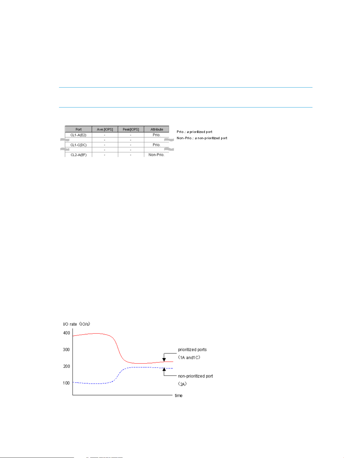
1. Set priority to ports on the storage system using the Port tab of the Performance Control main
window.
In network A, the ports 1A and 1C are connected to high-priority production servers. The port
2A is connected to a low-priority development server. Therefore, the ports 1A and 1C should
be given high priority, and the port 2A should be given low priority.
The next figure shows a portion of the Performance Control main window where the
abbreviation Prio. indicates that the associated port is given high priority, and the abbreviation
Non-Prio. indicates that the port is given low priority.
NOTE: The term prioritized port is used to refer to a high-priority port, and the term
non-prioritized port is used to refer to a low-priority port.
Figure 11 Priority specified in the Performance Control main window
2. Monitor traffic at ports. You must obtain statistics about traffic at each port on the storage
system.
There are two types of traffic statistics: the I/O rate and the transfer rate. The I/O rate is the
number of I/Os per second. The transfer rate is the size of data transferred between a host
and the storage system. When you view traffic statistics in the window, you select either the
I/O rate or the transfer rate. Use the Performance Monitor window of Performance Monitor
to view a line graph illustrating changes in traffic.
The next figure shows the changes in the I/O rate for the three ports (1A, 1C, and 2A).
According to the graph, the I/O rate for 1A and 1C was approximately 400 IO/s at first.
The I/O rate for 2A was approximately 100 IO/s at first. However, as the I/O rate for 2A
gradually increased from 100 IO/s to 200 IO/s, the I/O rate for 1A and 1C decreased from
400 IO/s to 200 IO/s. This fact indicates that the high-priority production servers have suffered
lowered performance. If you were the network administrator, you probably would like to
maintain the I/O rate for prioritized ports (1A and 1C) at 400 IO/s. To maintain the I/O rate
at 400 IO/s, you must set an upper limit to the I/O rate for the port 2A.
For detailed information about monitoring traffic, see “Setting priority for ports on the storage
system” (page 54) and “Analyzing traffic statistics” (page 54).
Figure 12 Traffic at ports
48 Performance Control operations
Page 49

3. Set an upper limit to traffic at the non-prioritized port. To prevent decline in I/O rates at
prioritized ports, you set upper limit values to the I/O rate for non-prioritized ports.
When you set an upper limit for the first time, it is recommended that the upper limit be
approximately 90 percent of the peak traffic. In network A, the peak I/O rate for the
non-prioritized port (2A) is 200 IO/s. So, the recommended upper limit for 2A is 180 IO/s.
For details on how to set an upper limit, see “Setting upper-limit values for non-prioritized
WWNs” (page 61).
4. Check the result of applying upper limit values. After applying upper limit values, you must
measure traffic at ports. You must view traffic statistics for prioritized ports 1A and 1C to check
whether the host performance is improved to a desirable level.
In network A, the desirable I/O rate for ports 1A and 1C is 400 IO/s. If the I/O rate reaches
400 IO/s, production server performance has reached to a desirable level. If production
server performance is not improved to a desirable level, you can change the upper limit to a
smaller value and then apply the new upper limit to the storage system. In network A, if the
upper limit is set to 180 IO/s but the I/O rate for 1A and 1C is still below 400 IO/s, the
administrator needs to change the upper limit until the I/O rate reaches 400 IO/s.
5. If necessary, apply a threshold. If you want to use threshold control, set threshold values in
the Port tab in the Performance Control main window. You can set threshold values in either
of the following ways:
• Set one threshold to each prioritized port
In network A, if you set a threshold of 200 IO/s to the port 1A and set a threshold of
100 IO/s to the port 1C, the upper limit on the non-prioritized port (2A) is disabled when
either of the following conditions is satisfied:
The I/O rate for the port 1A is 200 IO/s or lower.
The I/O rate for the port 1C is 100 IO/s or lower.
• Set only one threshold to the entire storage system
In network A, if you set a threshold of 500 IO/s to the storage system, the upper limit on
the non-prioritized port (2A) is disabled when the sum of the I/O rates for all prioritized
ports (1A and 1C) goes below 500 IO/s.
For details on how to set a threshold, see “Setting a threshold ” (page 56).
If many-to-many connections link HBAs and ports
The next figure shows an example of a network in which a production server and a development
server are connected to the storage system (Henceforth, this network is referred to as network B).
The host bus adapter (wwn01) in the production server is connected to four ports (1A, 1C, 2A and
2C). The host bus adapters (wwn02 and wwn03) in the development server are also connected
to the four ports.
If many-to-many connections link HBAs and ports 49
Page 50
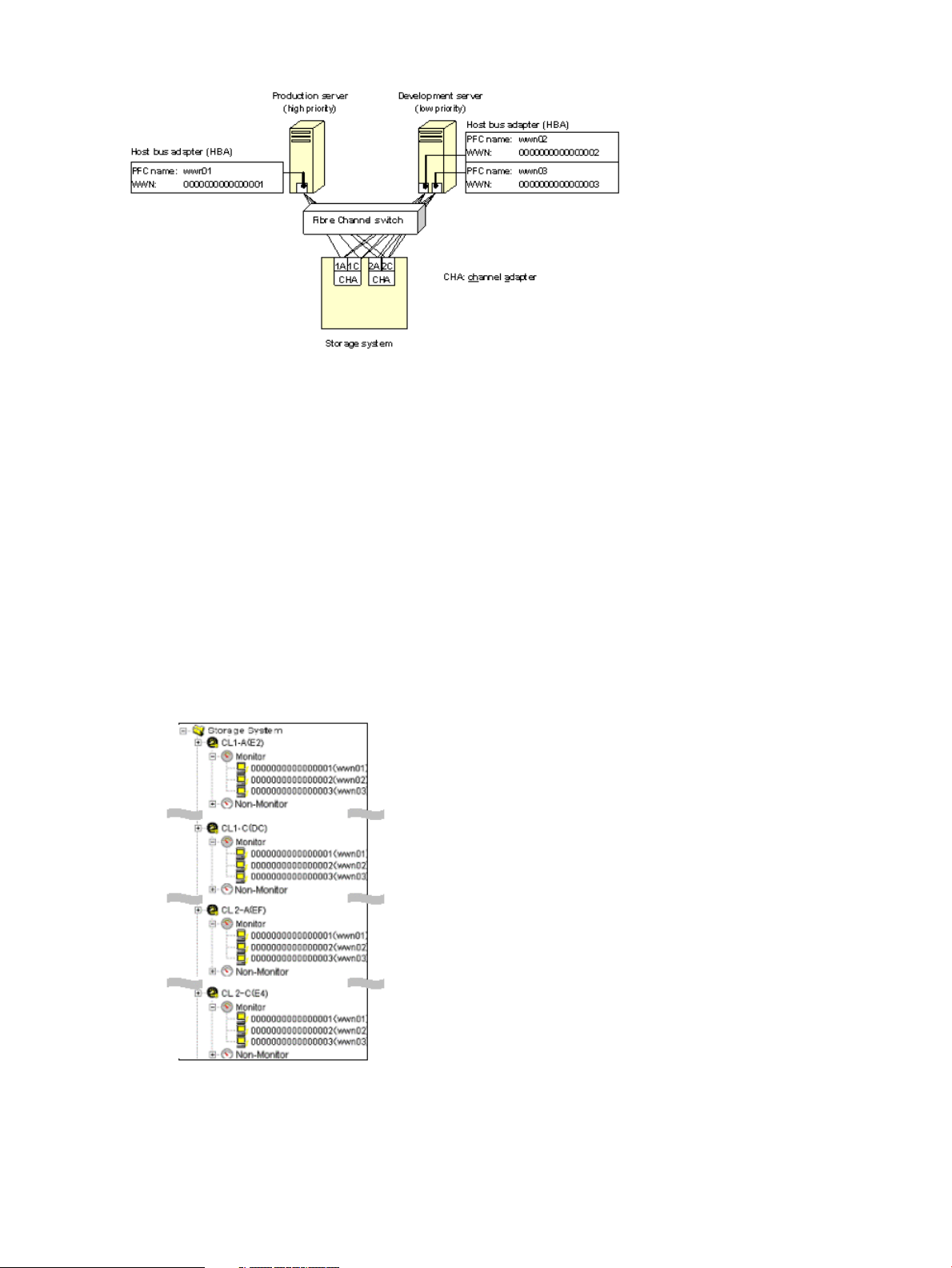
Figure 13 Network B (many-to-many connections are established between HBAs and ports)
If many-to-many connections are established between HBAs and ports, take the next steps:
1. Find WWNs of host bus adapters. Before using Performance Control, you must find the WWN
(Worldwide Name) of each host bus adapter in host servers. WWNs are 16-digit hexadecimal
numbers used to identify host bus adapters. For details on how to find WWNs, see the HP
XP P9000 Provisioning for Open Systems User Guide.
2. Ensure that all host bus adapters connected to ports in the storage system are monitored. Use
the WWN tab of the Performance Control main window to define which port is connected to
which host bus adapter. Place host bus adapters connected to each port below the Monitor
icons.
In network B, each of the four ports is connected to three host bus adapters (wwn01, wwn02,
and wwn03). Place the host bus adapter icons of wwn01, wwn02, and wwn03 below the
Monitor icons for all the four port icons.
The resulting definitions on the window are as follows:
Figure 14 Specifying host bus adapters to be monitored
For more detailed instruction, see “Setting priority for ports on the storage system” (page 54).
Performance Control is unable to monitor and control the performance of hosts whose host
bus adapters are placed below the Non-Monitor icon.
50 Performance Control operations
Page 51

3. Set priority to host bus adapters using the WWN tab of the Performance Control main window.
In network B, the production server is given high priority and the development server is given
low priority. If your network is configured as in Figure 13 (page 50), you must give high
priority to wwn01 and also give low priority to wwn02 and wwn03.
To give priority to the three host bus adapters, take the following steps:
• In the WWN tab, select one of the four ports that the HBAs are connected to (i.e., ports
1A, 1C, 2A, and 2C).
• Set Prio. to wwn01. Also, set Non-Prio. to wwn02 and wwn03.
Figure 15 Priority specified in the Performance Control main window
NOTE: The term prioritized WWN to refers to a high-priority host bus adapter (for example,
wwn01). The term non-prioritized port refers to a low-priority host bus adapter (for example,
wwn02 and wwn03).
4. Monitor traffic between host bus adapter and ports. You must obtain statistics about traffic
between host bus adapter and ports.
There are two types of traffic statistics: the I/O rate and the transfer rate. The I/O rate is the
number of I/Os per second. The transfer rate is the size of data transferred between a host
and the storage system. When you view traffic statistics in the window, you select either the
I/O rate or the transfer rate.
If your network is configured as network B, you must do the following:
• Measure traffic between the port 1A and the three host bus adapters (wwn01, wwn02
and wwn03.
• Measure traffic between the port 1C and the three host bus adapters (wwn01, wwn02
and wwn03.
• Measure traffic between the port 2A and the three host bus adapters (wwn01, wwn02
and wwn03.
• Measure traffic between the port 2C and the three host bus adapters (wwn01, wwn02
and wwn03.
The following graph illustrates the I/O rate at the paths between each port and the host
bus adapters. According to the graph, the I/O rate at the path between 1A and the
prioritized WWN (wwn01) was approximately 400 IO/s at first. The I/O rate at the
path between 1A and the non-prioritized WWNs (wwn02 and wwn03) was approximately
100 IO/s at first. However, as the I/O rate for non-prioritized WWNs (wwn02 and
wwn03) gradually increased from 100 IO/s to 200 IO/s, the I/O rate for the prioritized
WWN (wwn01) decreased from 400 IO/s to 200 IO/s. This indicates that the high-priority
production server has degraded. If you were the network administrator, you probably
would like to maintain the I/O rate for the prioritized WWN (wwn01) at 400 IO/s.
For more information about monitoring traffic, see “Setting priority for host bus adapters”
(page 60) and “Analyzing traffic statistics” (page 59).
If many-to-many connections link HBAs and ports 51
Page 52

Figure 16 Traffic at ports
5. Set an upper limit to traffic between ports and the non-prioritized WWN to prevent decline
in I/O rates at prioritized WWNs.
When you set an upper limit for the first time, the upper limit should be approximately 90
percent of the peak traffic level.
In network B, the peak I/O rate at the paths between port 1A and the non-prioritized WWNs
(wwn02 and wwn03) is 200 IO/s. The peak I/O rate at the paths between port 1C and the
non-prioritized WWNs is also 200 IO/s. The peak I/O rate at the paths between port 2A
and the non-prioritized WWNs is also 200 IO/s. The peak I/O rate at the paths between
port 2C and the non-prioritized WWNs is also 200 IO/s. So, the recommended upper limit
for the non-prioritized WWNs is 720 IO/s (= 200 ´ 4 ´ 0.90).
If your network is configured as in Figure 13 (page 50), you must do the following in this
order:
• In the WWN tab, select one of the four ports that the HBAs are connected to (i.e., ports
1A, 1C, 2A, and 2C).
• Set an upper limit to the non-prioritized WWNs (wwn02 and wwn03).
The following figure is the result of setting the upper limit of 720 IO/s to the paths between
1A and the non-prioritized WWNs. For details on how to set an upper limit, see “Setting
upper-limit values for non-prioritized WWNs” (page 61).
Figure 17 Setting upper limits
6. Check the result of applying upper limit values. After applying upper limit values, you must
measure traffic at ports. View traffic statistics for the prioritized WWN to check whether the
host performance is improved to a desirable level.
In network B, the desirable I/O rate for the prioritized WWN is 400 IO/s. If the I/O rate
reaches 400 IO/s, production server performance has reached to a desirable level. If
production server performance is not improved to a desirable level, you can change the upper
limit to a smaller value and then apply the new upper limit to the storage system. In network
B, if the upper limit is set to 720 IO/s but the I/O rate for wwn01 is still below 400 IO/s,
the administrator needs to change the upper limit until the I/O rate reaches 400 IO/s.
52 Performance Control operations
Page 53

If an upper limit of the non-prioritized WWN is set to zero or nearly zero, I/O performance
might be lowered. If I/O performance is lowered, the host cannot be connected to the storage
system in some cases.
7. If necessary, apply a threshold. If you want to use threshold control, set a threshold in the
WWN tab in the Performance Control main window.
In the WWN tab, you can specify only one threshold for the entire storage system, regardless
of the number of prioritized WWNs. For example, if there are three prioritized WWNs in the
network and the threshold is 100 IO/s, the upper limit on the non-prioritized WWNs is
disabled when the sum of the I/O rates for all prioritized WWNs goes below 100 IO/s.
For details on how to set a threshold, see “Setting a threshold” (page 62).
CAUTION: If you enter zero (0) in a cell to disable the upper limit, the cell displays a hyphen
(-) and the threshold for the prioritized port becomes ineffective. If the thresholds of all the
prioritized ports are ineffective, threshold control will not be performed but upper limit control
will be performed.
The following table shows the relationship between thresholds of a prioritized WWN and the
upper limits of a non-prioritized WWN.
Table 5 Prioritized WWN threshold setting relationships
Threshold settings
Threshold Is Set to The
Prioritized WWN
The Prioritized WWN
Port tab operations
If one-to-one connections are established between host bus adapters (HBAs) and storage system
ports, use the Port tab in the Performance Control main window to do the following:
• Analyze traffic statistics
• Measure traffic between host bus adapters and storage system ports
A number other than zero is set to the upper
limit of the non-prioritized WWN
When thresholds are set to prioritized
WWNs, depending on the I/O rate or the
transfer rate, the following controls are
executed.
• If the total value of I/O rate or transfer rate
exceeds the threshold in all prioritized
WWNs, upper limits of all the
non-prioritized WWNs take effect.
• If the total value of I/O rate or transfer rate
goes below the threshold in all prioritized
WWNs, upper limits of all the
non-prioritized WWNs do not take effect.
The specified upper limit always takes effect.Threshold Is Not Set to
Zero is set to the upper limit of the
non-prioritized WWN
The threshold control of the prioritized WWN
is not executed.
• Set priority to ports on the storage system
• Set an upper limit to traffic at each non-prioritized port
• Set a threshold to the storage system or to each prioritized port, if necessary
If one-to-one connections are established between host bus adapters and ports, you should specify
the priority of I/O operations on each port. You can specify the upper limit values on the
non-prioritized ports, and if necessary, you can also specify the threshold values on the prioritized
ports. Moreover, you can use one threshold value applied for the entire storage system.
Port tab operations 53
Page 54

For details on the system configuration of one-to-one connections between host bus adapters and
ports, see “If one-to-one connections link HBAs and ports” (page 47). This topic explains operation
procedures you can perform for ports and the entire storage system.
Analyzing traffic statistics
The traffic statistics reveal the number of I/Os that have been made via ports. The traffic statistics
also reveal the amount of data that have been transferred via ports. You must analyze the traffic
statistics to determine upper limit values that should be applied to I/O rates or transfer rates for
non-prioritized ports.
The following is the procedure for using the Performance Control main window to analyze traffic
statistics. You can also use the Performance Monitor window to analyze traffic statistics. Performance
Monitor can display a line graph that indicates changes in traffic.
1. Click Reports > Performance Monitor> Performance Control to open the Performance Control
window.
2. Click to change to Modify mode.
3. In the Performance Control window, click Performance Control. The Performance Control main
window appears.
4. Select the Port tab.
5. Select All from the list at the top right corner of the window.
6. Do one of the following:
• To analyze I/O rates, select IOPS from the list at the upper left corner of the list.
• To analyze transfer rates, select MB/s from the list at the upper left corner of the list.
The list displays traffic statistics (i.e., the average and peak I/O rates or transfer rates)
of the ports.
7. Analyze the information in the list and then determine upper limit values that should be applied
to non-prioritized ports. If necessary, determine threshold values that should be applied to
prioritized ports. For details on the upper limit values and threshold values, see “If one-to-one
connections link HBAs and ports” (page 47).
Setting priority for ports on the storage system
If one-to-one connection is established between HBAs and ports, you need to measure traffic
between high-priority HBAs and prioritized ports. You also need to measure traffic between
low-priority HBAs and non-prioritized ports.
Prioritized ports are ports on which the processing has high priority and non-prioritized ports are
ports on which the processing has low priority. Specify a port that connects to a high-priority host
bus adapter as a prioritized port. Specify a port that connects to a low-priority host bus adapter
as a non-prioritized port.
1. Click Reports >Performance Monitor> Performance Control to open the Performance Control
window.
2. Click to change to Modify mode.
3. In the Performance Control window, click Performance Control. The Performance Control main
window appears.
4. Ensure that the Port tab is displayed.
5. Select All from the list at the top right corner of the window.
6. Right-click a high-priority port and then select Non-Prio ->> Prio from the pop-up menu. If there
is more than one high-priority port, repeat this operation. The Attribute column displays Prio.
54 Performance Control operations
Page 55

7. Right-click a low-priority port and then select Prio ->> Non-Prio from the pop-up menu. If there
is more than one low-priority port, repeat this operation.
The Attribute column displays Non-Prio.
You must set upper limit values for the Non-prio. specified ports. For detail about the setting
of upper limit values, see “Setting upper-limit values to traffic at non-prioritized ports” (page 55).
8. Click Apply. The settings on the window are applied to the storage system.
After priority has been set, you can implement the procedure for measuring traffic (I/O rates and
transfer rates). See “Monitoring operation” (page 28).
Setting upper-limit values to traffic at non-prioritized ports
After you analyze traffic statistics, you must set upper limit values to I/O rates or transfer rates for
non-prioritized ports. Upper limit values for I/O rates are used to suppress the number of I/Os
from the low priority host servers and thus provide better performance for high-priority host servers.
Upper limit values for transfer rates are used to suppress the amount of data that should be
transferred between the storage system and the low priority ports, and thus provide better
performance for high-priority host servers.
1. Click Reports > Performance Monitor> Performance Control to open the Performance Control
window.
2. Click to change to Modify mode.
3. In the Performance Control window, click Performance Control. The Performance Control main
window appears.
4. Select the Port tab.
5. Do one of the following:
• To limit the I/O rate for the non-prioritized port, select IOPS from the list at the upper left
corner of the list.
• To limit the transfer rate for the non-prioritized port, select MB/s from the list at the upper
left corner of the list.
6. Locate the non-prioritized port in the list.
NOTE: The Attribute column of the list indicates whether ports are prioritized or non
prioritized. If you cannot find any non prioritized port in the list, check the list at the top right
corner of the window. If the list displays Prioritize, select All or Non Prioritize from the list.
7. Do one of the following:
• To limit the I/O rate for the non-prioritized port, double-click the desired cell in the IOPS
column in Upper. Next, enter the upper limit value in the cell.
• To limit the transfer rate for the non-prioritized port, double-click the desired cell in the
MB/s column in Upper. Next, enter the upper limit value in the cell.
In the list, either of IOPS or MB/s column is activated depending on the rate selected at
step 3 above. You can use either of them to specify the upper limit value for one port.
You can specify different types of rates (IOPS or MB/s) for the upper limit values of different
non-prioritized ports.
The upper limit value that you entered is displayed in blue.
8. Click Apply. The settings in the window are applied to the storage system. The upper limit
value that you entered turns black.
If an upper limit of the non-prioritized WWN is set to zero or nearly zero, I/O performance might
be lowered. If I/O performance is lowered, the host cannot be connected to the storage system
in some cases.
Port tab operations 55
Page 56

Setting a threshold
If threshold control is used, upper limit control is automatically disabled when traffic between
production servers and the storage system is reduced to a specified level. For details, see “Threshold
control” (page 9) and “If one-to-one connections link HBAs and ports” (page 47).
If one-to-one connections are established between HBAs and ports, you can set the threshold value
by the following two ways:
• Set a threshold value for each prioritized port
• Set one threshold value for the entire storage system
The procedures for these operations are explained below.
1. Click Reports > Performance Monitor> Performance Control to open the Performance Control
window.
2. Click to change to Modify mode.
3. In the Performance Control window, click Performance Control. The Performance Control main
window appears.
4. Select the Port tab.
5. To set a threshold value for each prioritized port, select the type of rates for the threshold value
from the list at the upper lest corner of the list.
• To use the I/O rates for the threshold value, select IOPS.
• To use the transfer rates for the threshold value, select MB/s.
NOTE: If you want to set one threshold value for the entire storage system, this step is
unnecessary.
6. Do one of the following:
• To set a threshold to each prioritized port, locate the desired prioritized port, which is
indicated by Prio. in the Attribute column. Next, double-click the cell in the IOPS or MB/s
column in Threshold, and then enter the threshold value. In the list, either of IOPS or MB/s
column is activated depending on the rate selected at step 5 above. Repeat this operation
to set the thresholds for all the prioritized ports. You can use different types of rates (IOPS
or MB/s) for thresholds of different prioritized ports.
CAUTION: If you enter zero (0) in a cell to disable the upper limit, the cell displays a
hyphen (-) and the threshold for the prioritized port becomes ineffective. If the thresholds
of all the prioritized ports are ineffective, threshold control will not be performed but upper
limit control will be performed. If you set thresholds for multiple prioritized ports and the
I/O rate or transfer rate becomes below the threshold at one of the prioritized port,
threshold control works in the entire storage system and the upper limits of the
non-prioritized ports are disabled. The following table shows the relationship between
the thresholds and the upper limits.
56 Performance Control operations
Page 57

Table 6 Relationship between the thresholds of the prioritized port and the upper limits
of the non-prioritized port
Thresholds settings
Threshold Is Set to
The Prioritized port
A number other than zero is set to the upper
limit of the non-prioritized port
When thresholds are set to multiple prioritized
ports, depending on the transfer rate, following
controls are executed.
Zero is set to the upper limit of the
non-prioritized port
The threshold control of the prioritized
port is not executed.
◦ If I/O rate or transfer rate exceeds the
threshold in any prioritized port, upper limits
of all the non-prioritized ports take effect.
◦ If I/O rate or transfer rate goes below the
threshold in any prioritized port, upper limits
of all the non-prioritized ports do not take
effect.
The specified upper limit always takes effect.Threshold Is Not
Set to The
Prioritized port
• To set one threshold to the entire storage system, select the All Thresholds check box.
Next, select IOPS or MB/s from the list of right side in All Thresholds and enter the threshold
value in the text box. Even if the types of rates for upper limit values and the threshold
are different, the threshold control can work for all the non-prioritized ports.
7. Click Apply. The settings in the window are applied to the storage system.
WWN tab operations
If many-to-many connections are established between host bus adapters (HBAs) and storage system
ports, you use the WWN tab in the Performance Control main window to do the following:
• Make all the traffics between host bus adapters and ports monitored
• Analyze traffic statistics
• Measure traffic between host bus adapters and storage system ports
• Set priority to host bus adapters
• Set an upper limit on traffic at non-prioritized WWNs
• Set a threshold, if necessary
If many-to-many connections are established between host bus adapters and ports, you should
specify the priority of I/O operations on each host bus adapter. You can specify the upper limit
values on the non-prioritized WWNs. If necessary, you can set one threshold value applied for
the entire storage system. When many-to-many connections are established between host bus
adapters and ports, you cannot set individual thresholds for prioritized WWNs.
For the system configuration of many-to-many connections between host bus adapters and ports,
see “If many-to-many connections link HBAs and ports” (page 49).
For details on the system configuration of many-to-many connections between host bus adapters
and ports, see “If many-to-many connections link HBAs and ports” (page 49). This topic explains
operation procedures you can perform for host bus adapters and the entire storage system.
Monitoring all traffic between HBAs and ports
When many-to-many connections are established between host bus adapters (HBAs) and ports,
you should make sure that all the traffic between HBAs and ports is monitored.
1. Click Reports > Performance Monitor> Performance Control to open the Performance Control
window.
WWN tab operations 57
Page 58

2. Click to change to Modify mode.
3. In the Performance Control window, click Performance Control. The Performance Control main
window appears.
4. Ensure that the WWN tab is visible.
The two trees are displayed in the left side of the WWN tab. The upper-left tree lists ports in
the storage system.
5. Select All from the list at the top right corner of the window.
6. In the upper-left tree, double-click a port.
7. Double-click Non-Monitor below the specified port.
If there are any host bus adapters whose traffics with the specified port are not monitored,
those host bus adapters are displayed below Non-Monitor.
8. Right-click Monitor and then select Add WWN.
The Add WWN window opens where you can add a WWN of a host bus adapter to Monitor.
9. In the Add WWN window, specify the WWN and the PFC name.
Expand the WWN list to show the WWNs of the host bus adapters that are connected to the
port but are not monitored. These host bus adapters are the same as that displayed in step 7.
From that list, select a WWN and specify the PFC name (up to 64 characters).
We recommend that you specify the same names for the PFC names and the nicknames of
the host bus adapters for convenience of host bus adapter management. Nicknames are
aliases of host bus adapters defined by LUN Manager. In the Performance Monitor window,
not only PFC names but also nicknames are displayed as the aliases of host bus adapters
(WWNs) in the list. Therefore, if you specify both the same aliases, the management of the
host bus adapters is easier.
10. Click OK. The selected WWN (of the host bus adapter) is moved from Non-Monitor to Monitor.
If the specified host bus adapter is connected to other ports, after clicking OK, a message
appears asking whether to change the settings of that host bus adapter for other ports, too.
Make the same setting for all the ports.
11. Repeat step 8 to 10 to move all the host bus adapters displayed below Non-Monitor to below
Monitor.
If you disconnect a host that has been connected via a cable to your storage system or change
the port to the another port of the host, the WWN for the host will remain in the WWN list
of the WWN tab. If you want to delete the WWN from the WWN list, you can delete the
WWN by using LUN Manager. For detail information of the deleting old WWNs from the
WWN list, see the HP XP P9000 Provisioning for Open Systems User Guide.
12. Click Apply in the Performance Control main window. The settings on the window are applied
to the storage system.
58 Performance Control operations
Page 59

If you add a port or host bus adapter to the storage system after the settings above, the traffics
about connections to the newly added port or host bus adapter will not be monitored. In this case,
follow the procedure above again to make all the traffics between host bus adapters and ports
monitored.
Up to 32 host bus adapters (WWNs) can be monitored for one port. If more than 32 host bus
adapters are connected to one port, the traffics about some host bus adapters will be obliged to
be excluded from the monitoring target. Consider the intended use of each host, and move the
host bus adapters that are not necessary to monitor to Non-Monitor by completing the steps in the
following section.
Excluding traffic between a host bus adapter and a port from the monitoring target
1. Click Reports > Performance Monitor> Performance Control to open the Performance Control
window.
2. Click to change to Modify mode.
3. In the Performance Control window, click Performance Control. The Performance Control main
window appears.
4. Ensure that the WWN tab is displayed.
5. Select All from the list at the top right corner of the window.
6. In the upper-left tree, double-click a port to which more than 32 host bus adapters are
connected.
7. Double-click Monitor below the specified port.
8. Right-click the WWN of a host bus adapter you want to exclude from the monitoring target
and then select Delete WWN from the pop-up menu.
NOTE:
• If the selected host bus adapter is connected to multiple ports, when you select the host
bus adapter and select the Delete WWN pop-up menu, a message will appear that asks
you whether to move the host bus adapter from Monitor to Non-Monitor below all other
ports, too.
• If the selected host bus adapter is contained in an PFC group, a message will appear
that tell you to delete the host bus adapter from the PFC group on ahead. You cannot
move a host bus adapter which is contained in an PFC group from Monitor to Non-Monitor.
For details on how to delete a host bus adapter from an PFC group, see “Deleting an
HBA from an PFC group” (page 65).
9. Click OK for the confirmation message that asks you whether to delete the host bus adapter.
The deleted host bus adapter (WWN) is moved from Monitor to Non-Monitor.
10. Click Apply in the Performance Control main window.
The settings on the window are applied to the storage system.
Analyzing traffic statistics
The traffic statistics reveal the number of I/Os that have been made via ports from HBAs. They
also reveal the amount of data that have been transferred between ports and HBAs. You must
analyze the traffic statistics to determine upper limit values that should be applied to I/O rates or
transfer rates for low-priority HBAs.
The following is the procedure for using the Performance Control main window to analyze traffic
statistics. You can also use the Performance Monitor window to analyze traffic statistics. Performance
Monitor can display a line graph that indicates changes in traffic.
1. Click Reports > Performance Monitor> Performance Control to open the Performance Control
window.
WWN tab operations 59
Page 60

2. Click to change to Modify mode.
3. In the Performance Control window, click Performance Control. The Performance Control main
window appears.
4. Select the WWN tab.
5. Select All from the list at the top right corner of the window.
6. Do one of the following:
• To analyze I/O rates, select IOPS from the list at the upper left corner.
• To analyze transfer rates, select MB/s from the list at the upper left corner of the list.
7. Below the Storage System folder in the upper-left tree, click the icon of the port whose traffic
statistics you want to collect.
The list displays traffic statistics (I/O rates or transfer rates) about the host bus adapters that
connect to the selected port.
The following two types of traffic are shown. The traffic has attributes including the average
and maximum values.
• Traffic between the host bus adapter and the selected port (shown in Per Port)
• Sum of the traffic between the host bus adapter and all the ports connected to the host
bus adapter (shown in WWN Total)
NOTE: The traffic statistics only about the host bus adapters below Monitor appear in
the list.
The WWN Total traffic statistics will also be displayed in the list when you click an icon
in the lower left tree. If you click the Storage System folder in the lower left tree, the sum
of the traffic of the host bus adapters registered on each PFC group is displayed. For
details on PFC groups, see “Grouping host bus adapters” (page 65).
8. Analyze the information in the list and then determine upper limit values that should be applied
to non-prioritized WWNs. If necessary, determine threshold values that should be applied to
prioritized WWNs. For details, see “If many-to-many connections link HBAs and ports”
(page 49).
Setting priority for host bus adapters
If many-to-many connection is established between host bus adapters (HBAs) and ports, you need
to define the priority of WWNs, measure traffic between each HBA and the port that the HBA is
connected to, and analyze the traffics.
The host bus adapters (HBAs) are divided into two types: Prioritized WWNs and non-prioritized
WWNs. Prioritized WWNs are the host bus adapters that are used for the high-priority processing,
and non-prioritized WWNs are the host bus adapters that are used for the low-priority processing.
Specify a host bus adapter existed in a server, on which the high-priority processing is performed,
as a prioritized WWNs. Specify a host bus adapter existed in a server, on which the low-priority
processing is performed, as a non-prioritized WWNs.
1. Click Reports > Performance Monitor> Performance Control to open the Performance Control
window.
2. Click to change to Modify mode.
3. In the Performance Control window, click Performance Control. The Performance Control main
window appears.
4. Select the WWN tab.
5. Select All from the list at the top right corner of the window.
6. In the upper-left tree, double-click a port.
60 Performance Control operations
Page 61

7. Double-click Monitor, which is displayed below the specified port.
8. Check to see if all the WWNs of the host bus adapters to be controlled by using Performance
Control appear below Monitor.
If some of the WWNs are missing, use the procedure in “Monitoring all traffic between HBAs
and ports” (page 57) to move all WWNs to below Monitor.
9. Click Monitor to display the information of the host bus adapters that are monitored in the list
on the right of the tree.
10. Right-click a host bus adapter (WWN) in the list and then select Non-Prio ->> Prio from the
pop-up menu.
The Attribute column of the selected WWN in the list displays Prio. If you want to specify
more than one prioritized WWN, repeat this operation.
NOTE: You cannot change the priority of a WWN that is contained in an PFC group. For
details on how to change the attribute of a WWN contained in an PFC group, see “Switching
priority of an PFC group” (page 66).
11. Right-click a host bus adapter (WWN) in the list and then select Prio ->> Non-Prio from the
pop-up menu.
The Attribute column of the selected WWN in the list displays Non-Prio. If you want to specify
more than one non-prioritized WWN, repeat this operation.
NOTE: You cannot change the priority of a WWN which is contained in an PFC group. For
details on how to change the attribute of a WWN contained in an PFC group, see “Switching
priority of an PFC group” (page 66).
You must set upper limit values for the Non-prio. specified ports. For details, see “Setting
upper-limit values for non-prioritized WWNs” (page 61).
12. Repeat steps 6 to 11 for ports (except for the port selected in step 6).
If one host bus adapter is connected to multiple ports and you specify the priority of the host
bus adapter for one port, the specified priority will be also applied to the host bus adapter
settings for other connected ports automatically.
13. Click Apply in the Performance Control main window. The settings on the window are applied
to the storage system.
Follow the instructions in “Starting monitoring” (page 28) to measure traffic (that is, I/O rates and
transfer rates).
Setting upper-limit values for non-prioritized WWNs
After you analyze traffic statistics about prioritized WWNs and non-prioritized WWNs, you must
set upper limit values to I/O rates or transfer rates for non-prioritized WWNs. Upper limit values
for I/O rates are used to suppress the number of I/Os from the low priority host servers and thus
provide better performance for high-priority host servers. Upper limit values for transfer rates are
used to suppress the amount of data that should be transferred between the storage system and
the low priority ports, thus providing better performance for high-priority host servers.
TIP: To set the same upper limit value to more than one non-prioritized WWN, use an PFC group.
For details on PFC groups, see “Grouping host bus adapters” (page 65).
1. Click Reports > Performance Monitor> Performance Control to open the Performance Control
window.
2. Click to change to Modify mode.
WWN tab operations 61
Page 62

3. In the Performance Control window, click Performance Control. The Performance Control main
window appears.
4. Ensure that the WWN tab is displayed.
5. Do one of the following:
• To limit the I/O rate of the non-prioritized WWN, select IOPS from the list at the upper
left corner.
• To limit the transfer rate of the non-prioritized WWN, select MB/s from the list at the
upper left corner.
6. In the upper-left tree, click the icon of the port whose traffic you want to limit below the Storage
System folder.
The information about the host bus adapters which connect to the selected port is displayed
in the list.
7. Locate the non-prioritized WWN in the list.
NOTE:
• The Attribute column of the list indicates whether WWNs are prioritized or non-prioritized.
The Attribute column of a non-prioritized WWN displays Non-Prio.
• If you cannot find any non-prioritized WWN in the list, check the list at the top right
corner of the window. If the list displays Prioritize, select All or Non-Prioritize.
8. Do one of the following:
• To limit the I/O rate of the non-prioritized WWN, double-click the desired cell in the IOPS
column in Upper. Next, enter the upper limit value in the cell.
• To limit the transfer rate of the non-prioritized WWN, double-click the desired cell in the
MB/s column in Upper. Next, enter the upper limit value in the cell.
In the list, either of the IOPS cells or MB/s cells are activated depending on the rate you
specified in step 5. You can specify the limit value by using either of the I/O rate or
transfer rate for each host bus adapter. The upper limit value that you entered is displayed
in blue. It is allowed that you specify upper limit values by using the I/O rate for some
host bus adapters and specify them by using the transfer rate for the other host bus
adapters.
NOTE:
◦ You cannot specify or change the upper limit value of a host bus adapter which is
contained in an PFC group. The upper limit value of such a host bus adapter is
defined by the PFC group settings. For details on how to specify an upper limit value
for an PFC group, see “Setting an upper-limit value to HBAs in an PFC group”
(page 66).
◦ If one host bus adapter is connected to multiple ports and you specify an upper limit
value of the host bus adapter for one port, the specified upper limit value will be
applied to the host bus adapter settings for other connected ports automatically.
9. Click Apply.
The settings in the window are applied to the storage system. The upper limit value that you
entered turns black.
Setting a threshold
If threshold control is used, upper limit control is automatically disabled when traffic between
production servers and the storage system is reduced to a specified level. For details, see “Threshold
control” (page 9) and “If many-to-many connections link HBAs and ports” (page 49).
62 Performance Control operations
Page 63

If many-to-many connections are established between host bus adapters and storage system ports,
you can set one threshold value for the entire storage system. In this environment, you cannot set
individual threshold values for each prioritized WWN.
1. Click Reports > Performance Monitor> Performance Control to open the Performance Control
window.
2. Click to change to Modify mode.
3. In the Performance Control window, click Performance Control. The Performance Control main
window appears.
4. Select the WWN tab.
5. Select the All Thresholds check box.
6. Select IOPS or MB/s from the All Thresholds list, and do one of the following:
• To specify the threshold value by using the I/O rate, select IOPS from the list below the
check box.
• To specify the threshold value by using the transfer rate, select MB/s from the list below
the check box.
Even if the types of rates differ between the upper limit values and the threshold value,
the threshold control is effective for all the non-prioritized WWNs.
7. Enter the threshold in the text box of All Thresholds.
8. Click Apply.
The settings in the window are applied to the storage system.
Changing the PFC name of a host bus adapter
Use the Performance Control main window to assign an PFC name to a host bus adapter (HBA).
Although you can identify HBAs by WWNs (Worldwide Names), you will be able to identify HBAs
more easily if you assign PFC names. WWNs are 16-digit hexadecimal numbers and cannot be
changed. However, PFC names should not necessarily be 16-digit hexadecimal numbers and can
be changed.
The following is the procedure for changing an already assigned PFC name. For details on how
to assign an PFC name, see “Monitoring all traffic between HBAs and ports” (page 57).
1. Click Reports > Performance Monitor> Performance Control to open the Performance Control
window.
2. Click to change to Modify mode.
3. In the Performance Control window, click Performance Control. The Performance Control main
window appears.
4. Ensure that the WWN tab is displayed.
5. In the upper-left tree, select a host bus adapter ( ) from below Monitor and then right-click
the selection.
6. From the pop-up menu, select Change WWN and PFC Name. The Change WWN and PFC
Name window opens.
WWN tab operations 63
Page 64
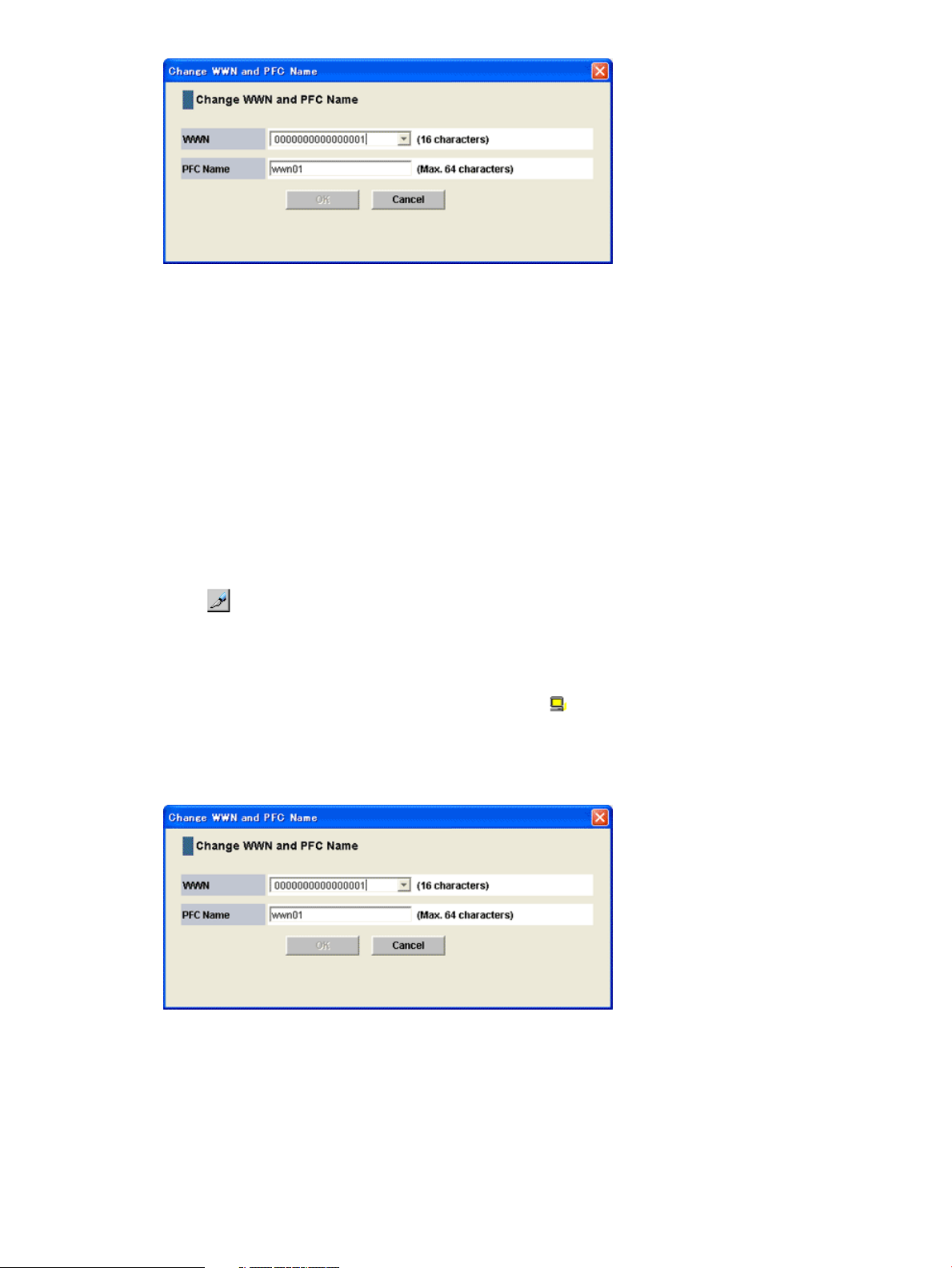
7. Enter a new PFC name in the PFC Name box and then select OK. You can use up to 64
characters for an PFC name.
8. In the Performance Control main window, click Apply. The settings in the window are applied
to the storage system.
Registering a replacement host bus adapter
If a host bus adapter fails, replace the adapter with a new one. After you finish replacement, you
will need to delete the old host bus adapter from the Performance Control main window and then
register the new host bus adapter.
When you add a new host bus adapter rather than replacing an old one, the WWN of the added
host bus adapter is automatically displayed below Non-Monitor for the connected port in the list.
1. Click Reports > Performance Monitor> Performance Control to open the Performance Control
window.
2. Click to change to Modify mode.
3. In the Performance Control window, click Performance Control. The Performance Control main
window appears.
4. Select the WWN tab.
5. In the upper-left tree, select the old host bus adapter ( ) from below Monitor and then right-click
the selection.
6. From the pop-up menu, select Change WWN and PFC Name. The Change WWN and PFC
Name window opens.
7. Enter the WWN of the new host bus adapter in the WWN combo box.
You can select the WWN of the newly connected host bus adapter in the WWN combo box.
8. If necessary, enter a new PFC name in the PFC Name box. You can use up to 64 characters
for an PFC name.
9. Select OK to close the Change WWN and PFC Name window.
10. In the Performance Control main window, click Apply. The settings in the window are applied
to the storage system.
64 Performance Control operations
Page 65

Grouping host bus adapters
Use Performance Control to create an PFC group to contain multiple host bus adapters. You can
include a maximum of 32 host bus adapters in a PFC group. You can create up to 512 PFC groups
in the storage system. All the host bus adapters (HBAs) in one PFC group must be of the same
priority. Prioritized WWNs and non-prioritized WWNs cannot be mixed in the same group.
You can use an PFC group to switch priority of multiple HBAs from prioritized to non-prioritized,
or vice versa. You can also use an PFC group to set the same upper limit value to all the HBAs in
the group.
Containing multiple HBAs in an PFC group
A host bus adapter can be contained in only one PFC group. To create an PFC group and contain
multiple host bus adapters in the group:
1. Click Reports > Performance Monitor> Performance Control to open the Performance Control
window.
2. Click to change to Modify mode.
3. In the Performance Control window, click Performance Control. The Performance Control main
window appears.
4. Select the WWN tab.
5. In the lower-left tree, select and right-click the Storage System folder.
6. From the pop-up menu, select Add New PFC Group.
7. In the Add New PFC Group window, enter the name of the PFC group and then select OK. An
PFC group is created and an PFC group icon ( ) is added to the lower-left tree.
8. Select an HBA from the upper-left tree and select an PFC group from the lower-left tree.
Next, click Add WWN.
Repeat this operation until all desired HBAs are added to the PFC group.
NOTE:
• Select a host bus adapter from below Monitor. You cannot add HBAs from below
Non-Monitor to PFC groups.
• When selecting a host bus adapter that is already contained in some PFC group from
the upper-left tree, the Add WWN button is not activated. Select a host bus adapter that
is not contained in any PFC groups.
9. Click Apply. The settings in the window are applied to the storage system.
Deleting an HBA from an PFC group
1. Click Reports > Performance Monitor> Performance Control to open the Performance Control
window.
2. Click to change to Modify mode.
3. In the Performance Control window, click Performance Control. The Performance Control main
window appears.
WWN tab operations 65
Page 66

4. Select the WWN tab.
5. In the lower-left tree, double-click the PFC group ( ) that contains the host bus adapter to be
deleted.
6. Below the PFC icon, right-click the icon the host bus adapter ( ) you want to delete.
7. Select Delete WWN from the pop-up menu.
The selected host bus adapter icon is deleted from the tree.
8. Click Apply. The settings on the window are applied to the storage system.
Switching priority of an PFC group
All the host bus adapters (HBAs) in one PFC group must be of the same priority. Prioritized WWNs
and non-prioritized WWNs cannot be mixed in one PFC group.
You can use an PFC group to switch priority of multiple HBAs from prioritized to non-prioritized,
or vice versa.
1. Click Reports > Performance Monitor> Performance Control to open the Performance Control
window.
2. Click to change to Modify mode.
3. In the Performance Control window, click Performance Control. The Performance Control main
window appears.
4. Select the WWN tab.
5. In the lower-left tree, select and right-click an PFC group ( ).
6. Do one of the following:
• To switch priority from prioritized to non-prioritized, select Prio ->> Non-Prio from the
pop-up menu.
• To switch priority from non-prioritized to prioritized, select Non-Prio ->> Prio from the
pop-up menu.
7. Click Apply. The settings in the window are applied to the storage system.
Setting an upper-limit value to HBAs in an PFC group
If all the host bus adapters in an PFC group are non-prioritized WWNs, you can set an upper limit
value to HBA performance (i.e., I/O rate or transfer rate). You can assign one upper limit value
for one PFC group.
For example, suppose that the upper limit value 100 IOPS is assigned to an PFC group consisting
of four host bus adapters. If the sum of the I/O rate of the four HBAs reaches 100 IOPS, Performance
Control controls the system so that the sum of the I/O rates will not exceed 100 IOPS.
1. Click Reports > Performance Monitor> Performance Control to open the Performance Control
window.
2. Click to change to Modify mode.
3. In the Performance Control window, click Performance Control. The Performance Control main
window appears.
4. Select the WWN tab.
5. In the lower-left tree, select and right-click the Storage System folder or an PFC group ( ).
66 Performance Control operations
Page 67
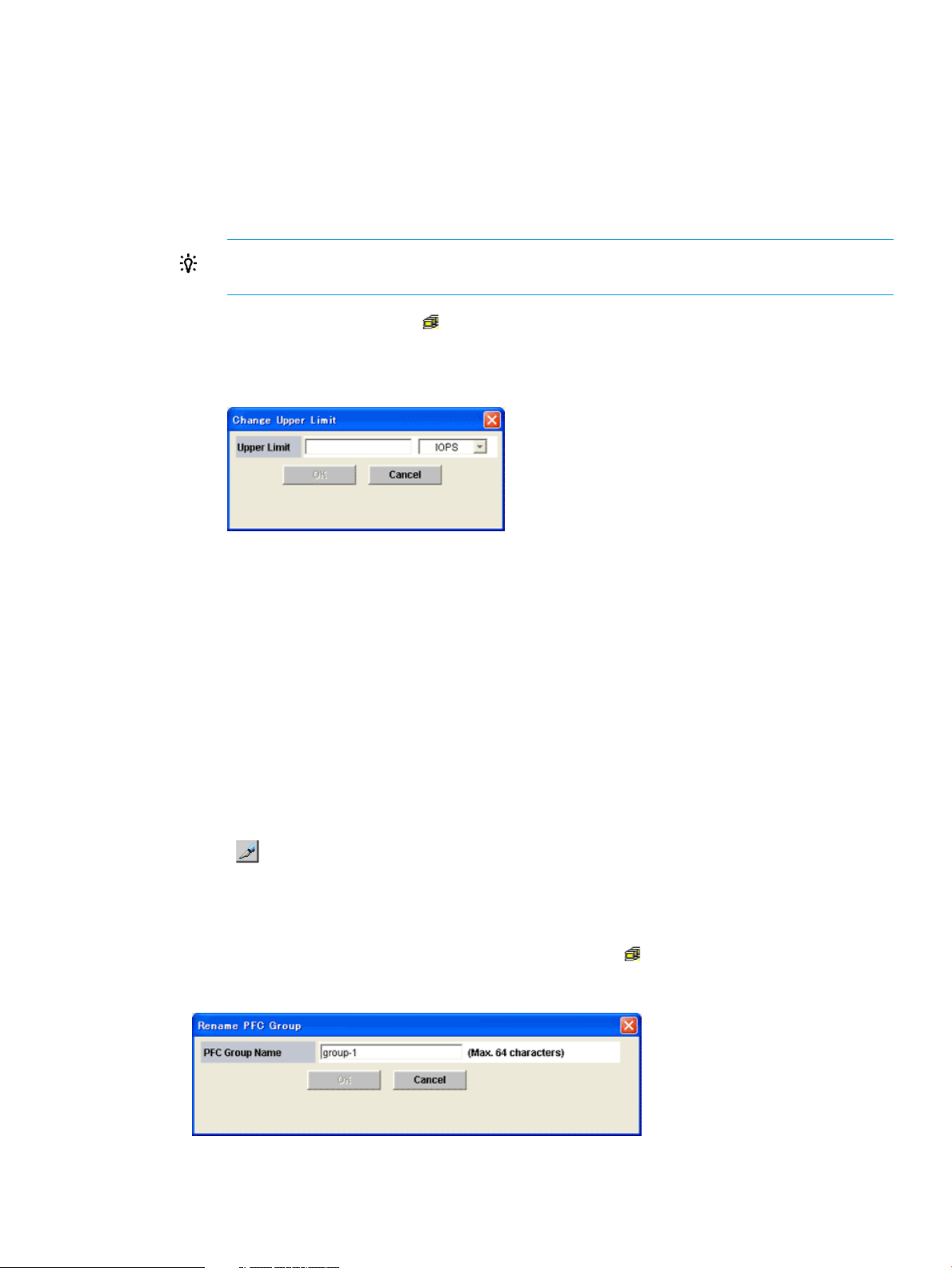
6. If you selected the Storage System folder, take the following steps:
• Select IOPS or MB/s from the list at the upper-left corner of the list. Select IOPS if you
want to assign an upper limit to the I/O rate. Select MB/s if you want to assign an upper
limit to the transfer rate.
• To assign an upper limit to the I/O rate, enter the upper limit value in the IOPS column
of the list. To assign an upper limit to the transfer rate, enter the upper limit value in the
MB/s column of the list.
TIP: If you cannot see the IOPS or MB/s column, scroll the list to the left. The column is
located at the right side of the list.
If you selected an PFC group ( ), take the following steps:
• Right-click the selected PFC group and then select Change Upper Limit from the pop-up
menu. The Change Upper Limit dialog box opens.
• To assign an upper limit to the I/O rate, enter the upper limit value and then select IOPS
from the list. Next, select OK. To assign an upper limit to the transfer rate, enter the upper
limit value and then select MB/s from the list. Next, select OK.
7. In the Performance Control main window, click Apply. The settings in the window are applied
to the storage system.
To confirm an upper limit value specified for each PFC group, select the Storage System folder
in the lower-left tree of the WWN tab. The PFC groups are displayed in the list and you can
confirm each upper limit value.
Renaming an PFC group
1. Click Reports > Performance Monitor> Performance Control to open the Performance Control
window.
2. Click to change to Modify mode.
3. In the Performance Control window, click Performance Control. The Performance Control main
window appears.
4. Select the WWN tab.
5. In the lower-left tree, select and right-click an PFC group ( ).
6. Select Rename PFC Group from the pop-up menu. The Rename PFC Group dialog box opens.
7. Enter the new name and select OK.
WWN tab operations 67
Page 68

8. In the Performance Control main window, click Apply.
The settings in the window are applied to the storage system.
Deleting an PFC group
1. Click Reports > Performance Monitor> Performance Control to open the Performance Control
window.
2. Click to change to Modify mode.
3. In the Performance Control window, click Performance Control. The Performance Control main
window appears.
4. Select the WWN tab.
5. In the lower-left tree, select and right-click an PFC group ( ).
6. Select Delete PFC Group from the pop-up menu.
7. In the Performance Control main window, click Apply. The settings in the window are applied
to the storage system.
68 Performance Control operations
Page 69

11 Estimating cache size
This topic describes how to estimate the cache size required for using Cache Residency.
About cache size
The required cache size for using Cache Residency differs according to operation modes or RAID
levels. For example, if the bind mode is set, RAID1 storage systems require twice the size of cache
for the user data to use Cache Residency. However, RAID5 or RAID6 storage systems require three
times the size of cache. If external volumes are used, twice the cache size for the user data is
required to use Cache Residency.
NOTE: If a RAID5 or RAID6 volume area is changed from priority mode to bind mode and no
cache is added, then only 33% of the user data will fit in the area previously assigned for priority
mode, and the remaining 67% is used to save read/write data.
If a RAID1 volume area is changed from priority mode to bind mode and no cache is added, then
only 50% of the user data will fit in the area previously assigned for priority mode, and the
remaining 50% is used to save read/write data.
Changing the mode without cache extension requires reconfiguring Cache Residency.
About cache size 69
Page 70

If the priority mode or the bind mode is set, the cache size is calculated assuming that one slot has
the following values.
• For open-systems volumes:
For OPEN-V, one slot is 264 KB (512 LBAs).◦
◦ For other than OPEN-V, one slot is 66 KB (128 LBAs).
• For mainframe (3390) volumes:
◦ One slot is 66 KB (128 LBAs).
Calculating cache size for open systems
70 Estimating cache size
Page 71

1. Calculate the converted values of the starting address and the ending address.
For all specified LDEVs:
1. For OPEN-V:
Number of LBAs = LDEV size (KB)×2
Convert the LDEV size to the number of LBAs.
Number of slots = ceil (Number of LBA ÷ 512)
Round up the value that is calculated from the formula enclosed by ceil().
Converted value of starting address = 0
Converted value of ending address = (Number of slots × 512) - 1
2. For emulation types other than OPEN-V:
Number of LBAs = LDEV size (KB) × 2
Convert the LDEV size to the number of LBAs
Number of slots = ceil (Number of LBAs ÷ 96)
Round up the value that is calculated from the formula enclosed by ceil().
Converted value of starting address = 0
Converted value of ending address = (Number of slots × 96) - 1
If the volumes are specified:
1. for OPEN-V:
Starting value = floor (Setting value of starting address (LBA) ÷ 512)
Round down the value that is calculated from the formula enclosed by floor(). "Setting
value of starting address (LBA)" is the value which is input on the Cache Residency
window.
Ending value = floor (Setting value of ending address (LBA) ÷ 512)
Round down the value that is calculated from the formula enclosed by floor(). "Setting
value of ending address (LBA)" is the value which is input on the Cache Residency window.
Converted value of starting address = Starting value × 512
Converted value of ending address = ((Ending value + 1) × 512) - 1
2. For emulation types other than OPEN-V:
Starting value = floor (Setting value of starting address (LBA) ÷ 96)
Round down the value that is calculated from the formula enclosed by floor(). "Setting
value of starting address (LBA)" is the value which is input on the Cache Residency
window.
Ending value = floor (Setting value of ending address (LBA) ÷ 96)
Round down the value that is calculated from the formula enclosed by floor(). "Setting
value of ending address (LBA)" is the value which is input on the Cache Residency window.
Converted value of starting address = Starting value × 96
Converted value of ending address = ((Ending value + 1) × 96) - 1
2. Calculate the number of addresses between the starting address and the ending address
calculated in step 1.
1. For OPEN-V:
Number of addresses = Converted value of ending address - Converted value of starting
address + 1
Calculate the number of LBAs that are used by the user data.
Calculating cache size for open systems 71
Page 72

2. For emulation types other than OPEN-V:
Number of LBAs = Converted value of ending address - Converted value of starting
address + 1
Calculate the number of LBAs that are used by the user data.
Number of slots = Number of LBAs ÷96
Convert the number of LBAs to the number of slots.
Number of addresses = Number of slots × 128
Convert the number of slots with 128 LBA.
3. Calculate the required cache size according to the operation modes, or the RAID levels to use
Cache Residency.
1. Where the bind mode is set:
For RAID1
Required cache size = No. of addresses × (512 + 16) × 2 ÷ 1,024
The unit is KB.
For RAID type other than RAID1:
Required cache size = No. of addresses × (512 + 16) × 3 ÷ 1,024
The unit is KB.
2. Where the priority mode is set:
Required cache size = Number of addresses × (512 + 16) ÷ 1,024
The unit is KB.
72 Estimating cache size
Page 73

Calculating cache size for mainframe systems
1. Calculate the converted values of the starting address and the ending address.
1. For all specified LDEVs:
Setting value of ending address (CC) = floor (((LDEV size × 15) - 1) ÷ 15)
Round down the value that is calculated from the formula enclosed by floor(). "Setting
value of ending address (CC)" is the value which is input on the Cache Residency window.
Setting value of ending address (HH) = ((LDEV size × 15) - 1) Mod 15
The remainder will be the setting value of ending address (HH).
"Setting value of ending address (HH)" is the value which is input on the Cache Residency
window.
Converted value of starting address = 0
Converted value of ending address = Setting value of ending address (CC) × 15 + Setting
value of ending address (HH)
"Setting value of ending address (CC)" and "Setting value of ending address (HH)" is
the value which is input on the Cache Residency window.
2. If the volumes are specified:
Converted value of starting address = Setting value of starting address (CC) × 15 +
Setting value of starting address (HH)
"Setting value of ending address (CC)" and "Setting value of ending address (HH)" is
the value which is input on the Cache Residency window.
Converted value of ending address = Setting value of ending address (CC) × 15 + Setting
value of ending address (HH)
"Setting value of ending address (CC)" and "Setting value of ending address (HH)" is
the value which is input on the Cache Residency window.
2. Calculate the number of addresses between the starting address and the ending address
calculated in step 1:
Number of addresses = Converted value of ending address - Converted value of starting
address + 1
Calculate the number of addresses of cache that are used by the user data.
3. Calculate the required cache size according to the operation modes, or the RAID levels to use
Cache Residency.
1. Where the bind mode is set:
For RAID1
Required cache size = (Number of addresses × ((128 × (512 + 16)) × 2) ÷ 1,024
The unit is KB.
2. Where the priority mode is set:
Required cache size = (Number of addresses × (128 × (512 + 16))) ÷ 1,024
The unit is KB.
Cache Residency cache areas
The Cache Residency cache areas have the following parameters:
• The cache areas are dynamic and can be added and deleted at any time.
• The HP XP P9500 supports a maximum of 1,024 addressable cache areas per LDEV and per
storage system.
Calculating cache size for mainframe systems 73
Page 74

• For OPEN-V volumes, Cache Residency cache areas must be defined in logical blocks using
logical block addresses (LBAs), with a minimum size of 512 LBAs (equivalent to 264 KB). In
most cases you will assign an entire open-systems volume for cache residency. If the remaining
cache memory is less than 256 MB, Cache Residency is not available.
• For mainframe volumes, Cache Residency cache areas must be defined on contiguous tracks
with a minimum size of one cache slot (or track) (equivalent to 66 KB) and a maximum size
of one LVI.
• You can prestage the data to the resident cache area. If prestaging is not used, the data will
be loaded into the Cache Residency area when the first “miss” occurs. If prestaging is used,
performance may be affected for a short time while the data is read into Cache Residency
cache.
CAUTION: Prestaging of Cache Residency data should not be performed during peak
activity.
• All write I/Os to Cache Residency data are duplex writes, guaranteeing full data integrity.
The Cache Residency data remains fixed in cache until you manually delete it. Deletion of
Cache Residency cache areas destages any write data to the affected volumes.
• It is possible to expand the amount of Cache Residency cache without canceling the existing
Cache Residency settings. For details, contact HP Technical Support.
Cache Residency system specifications
types
Unit of cache area allocation
SpecificationItem
OPEN-3, 8, 9, E, L
Virtual LUN volume
For OPEN-V, at least 512 LBAs:
Equivalent to 264 KB
For other than OPEN-V, at least 96 LBAs:
Equivalent to 66 KB
Per storage system: 16,384Number of cache areas
Per LDEV: 4,096
Minimum 512 MBTotal cache capacity
Mainframe systemOpen system
3380-3, 3A, 3B, 3C,OPEN-VSupported device emulation
3390-3, 3A, 3B, 3C, 3R, 9, 9A, 9B, 9C, L,
LA, LB, LC, M, MA, MB, MC, A
Virtual LVI volumeLUN Expansion (LUSE) volumeSupported volume types
At least one cache slot (or track): Equivalent
to 66 KB.Up to 1 LDEV.
74 Estimating cache size
Page 75

12 Managing resident cache
This topic provides instructions for using Cache Residency software to manage resident cache.
Cache Residency rules, restrictions, and guidelines
Rules
• Cache Residency must be enabled on Remote Web Console.
• Administrator or Cache Residency write access to the Remote Web Console software is required
to perform Cache Residency operations. Users without write access can view Cache Residency
information for the connected storage system but cannot set or change options.
• Do not attempt to allocate Cache Residency cache beyond the allocated capacity.
• Do not apply Cache Residency settings to volumes reserved for Auto LUN V2.
• Do not attempt to allocate Cache Residency cache redundantly over the cache area that is
already allocated to an LDEV.
• Do not apply or refer to Cache Residency settings to volumes from the host and Remote Web
Console at the same time. You can apply the settings from the host if you use Cache Manager.
• If you specify the Cache Residency setting on the volume during quick formatting, do not use
the prestaging function. If you want to use the prestaging function after the quick formatting
processing completes, release the setting and then specify the Cache Residency setting again,
with the prestaging setting enabled this time. For information about quick formatting, see the
HP XP P9000 Provisioning for Open Systems User Guide or the HP XP P9000 Provisioning
for Mainframe Systems User Guide.
• Do not perform the Business Copy quick restore operation or the Auto LUN V2 operation on
a Cache Residency volume. Also, do not specify the Cache Residency setting on the volume
on which the Business Copy quick restore or Auto LUN V2 operation is performed. These
operations swap the internal locations of the source and target volumes, which causes a loss
of data integrity. For additional information, see the HP XP P9000 Business Copy User Guide,
the HP XP P9000 Business Copy for Mainframe User Guide, and/or contact HP Technical
Support.
• To set Cache Residency for a LUSE volume, you must set Cache Residency for an LDEV that
is a component of the LUSE volume. To determine the LDEV for which you want to set Cache
Residency, you must know the exact number of LBAs in each LDEV that is a component of the
LUSE volume.
NOTE: The number of LBAs displayed on the Cache Residency window is different from the
actual number of LDEVs, and does not match the number of LBAs recognized by the host.
To identify the exact number of LBAs in a LDEV, first display the Remote Web Console main
window and search for the parity group to which the LDEV belongs according to the LDKC,
control unit (CU), and LDEV numbers. For further information about the Basic Information
Display window, see the HP XP P9000 Remote Web Console User Guide.
As shown in Figure 18 (page 76), the LUSE volume is composed of three LDEVs, for example,
00:01 (1,000 LBAs), 00:02 (1,002 LBAs), and 00:03 (1,020 LBAs). If you see from the host
and want to set Cache Residency to 500 LBAs starting from No. 1,020 LBA, you may set the
Cache Residency to 500 LBAs starting from No. 20 LBA of the 2nd LDEV because the first
LDEV size is 1,000 LBAs.
Cache Residency rules, restrictions, and guidelines 75
Page 76
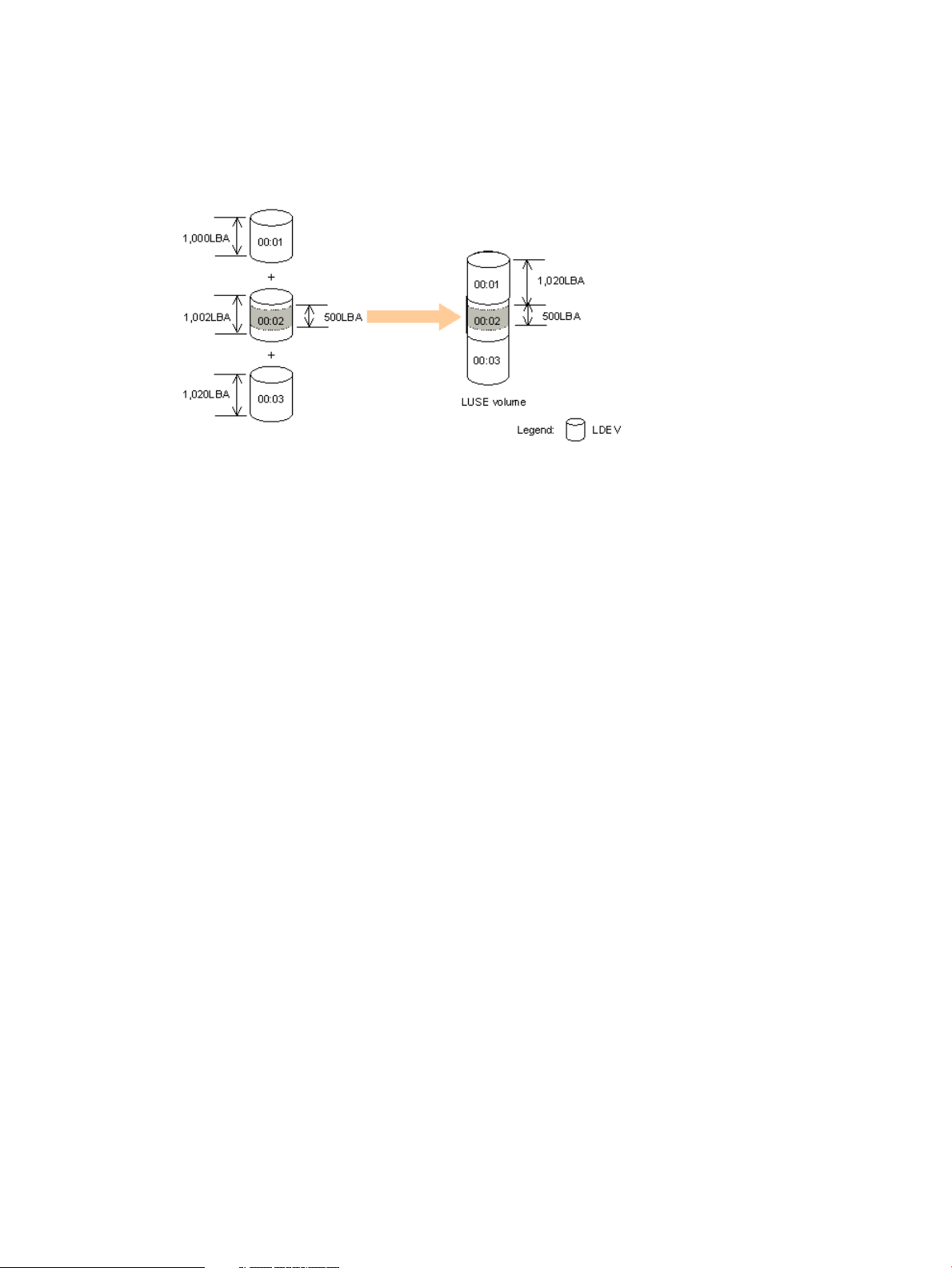
The following operations automatically reset Cache Residency cache:
◦ When LDEVs that is partly or wholly assigned to Cache Residency is deleted.
◦ When the parity group containing LDEVs that are assigned to Cache Residency is deleted.
Figure 18 Example of LBA Value Setting When Using LUSE
Restrictions
• The Cache Residency bind mode is not available to external volumes whose Cache mode is
set to Disable (which is the mode that disables the use of the cache when there is an I/O
request from the host).
• You cannot allocate pool-VOLs and V-VOLs for Cache Residency. For further information about
pool-VOLs and V-VOLs, see the HP XP P9000 Snapshot User Guide, the HP XP P9000
Provisioning for Open Systems User Guide, or the HP XP P9000 Provisioning for Mainframe
Systems User Guide
• You cannot allocate the journal volumes for Cache Residency. For additional information
about the journal volumes, see the HP XP P9000 Continuous Access Journal User Guide or
the HP XP P9000 Continuous Access Journal for Mainframe Systems User Guide.
• You cannot allocate the remote command device for Cache Residency. For further information
about the remote command device, see the HP XP P9000 External Storage for Open and
Mainframe Systems User Guide.
• You cannot allocate a quorum disk for Cache Residency.
• You cannot allocate the nondisruptive migration volumes for Cache Residency.
Guidelines
• Performing Cache Residency operations on many LDEVs during host I/O may cause the host
I/O response time to become slow. To avoid degradation of response time, set only one LDEV
at a time.
• Deleting data from cache during host I/O may cause the response time of host I/O to become
slow. To avoid degradation of host response time, limit the amount of data you delete in one
operation as follows:
If the host timeout period is set to 10 seconds or shorter, limit the total amount of data to:
◦ 1 GB or less for open systems
◦ 1,000 cylinders or less for mainframe systems
76 Managing resident cache
Page 77

If the host timeout period is set to 11 seconds or longer, limit the total amount of data to:
◦ 3 GB or less for open systems
◦ 3,000 cylinders or less for mainframe systems
Launching Cache Residency
1. Log on to the primary SVP.
2. On the menu bar of the Remote Web Console main window, click Actions > Other function
> Cache Residency.
3. In the Cache Residency window, change from View to Modify mode.
Viewing Cache Residency information
The Cache Residency information can be viewed in the following fields in the Cache Residency
window:
• CU:LDEV tree
• LDEV information table
• Cache information area
Placing specific data into Cache Residency cache
This procedure places specific data from one or more LDEVs into Cache Residency cache.
1. In the Cache Residency window, select the desired CLPR from the CLPR: list.
2. In the CU:LDEV tree, select the LDKC and the CU containing the desired LDEV, and then select
the desired LDEV.
The LDEV information table shows the information for the selected LDEV. A dash (-) in the Mode
column indicates an area not already allocated to Cache Residency cache.
Launching Cache Residency 77
Page 78

3. Select an unallocated area in the LDEV information table as the area to place specific data
from one or more LDEVs into Cache Residency cache. The starting and ending addresses of
the selected area appear in the Start and End fields.
NOTE: For OPEN-V LUs, Cache Residency identifies a logical area in units of 512 blocks.
If you enter 0 or 1 as the starting LBA and a value less than 511 as the ending LBA, Cache
Residency automatically changes the ending block address to 511.
4. In the Cache Residency window, select options to apply to all selected LDEVs:
1. In the Cache Residency Mode box, select the desired mode (Bind or Priority).
2. Select the desired Prestaging Mode setting (Yes or No). To set the prestaging function,
the Prestaging check box must already be selected.
3. Verify the starting and ending addresses of the area to be placed in Cache Residency
cache in the Start and End fields. Edit as needed. Make sure that the Select All Area box
is NOT checked.
CAUTION: Make sure to select the correct options because the options cannot be
changed after data is added to cache. To change between bind/priority modes, or to
enable/disable the prestaging function, release the cache extent that you want to change,
and then place the data back into Cache Residency cache with the desired settings.
5. If you do not want to apply the same options to any other LDEV, make sure that the Multi Set
/ Release box is not checked, click Set, and then click OK on the confirmation dialog box.
The requested Cache Residency operation appears in blue in the LDEV information table.
To apply the same options and data range to additional LDEVs:
1. On the Cache Residency window, select the Multi Set / Release box, click Set, and then
click OK. The Multi Set dialog box opens showing the data range and options selected
on the Cache Residency window.
2. In the Multi Set dialog box, select the desired LDKC and CU image, and select the desired
LDEVs. The data range and options displayed in the dialog box will be applied to all
selected LDEVs.
3. Click Set to return to the Cache Residency window. The requested Cache Residency
operations appear in blue in the LDEV information table.
6. Repeat steps 2 through 5 until all desired operations are listed. The Release is unavailable
until you apply (or cancel) your requested operations.
78 Managing resident cache
Page 79

7. Verify the Prestaging setting:
• To enable prestaging, select Prestaging.
• To disable prestaging, clear Prestaging.
8. To start the operations, click Apply. If Prestaging was selected, respond to the Yes/No
confirmation. To continue with prestaging, click Yes. To continue without it, click No.
9. Monitor the Cache Residency window to make sure that the operations complete successfully.
The cache information area shows the progress of the requested operations.
Placing LDEVs into Cache Residency cache
This procedure places all data on one or more LDEVs into Cache Residency cache.
1. In the Cache Residency window, select the desired CLPR from the CLPR list.
2. In the CU:LDEV tree, select the LDKC and the CU containing the desired LDEV, and then select
the desired LDEV.
The LDEV information table shows the information for the selected LDEV. A dash (-) in the Mode
column indicates an area not already allocated to Cache Residency cache.
3. In the Cache Residency window, select desired options:
1. In the Cache Residency Mode box, select the desired mode (Bind or Priority).
2. Select the desired Prestaging Mode setting (Yes or No). To set the prestaging function,
the Prestaging check box must already be selected.
3. Check the Select All Area box. Leave the Start and End fields blank.
CAUTION: Make sure to select the correct options, because the options cannot be
changed after data is added to cache. To change between bind and priority modes, or
to enable and disable the prestaging function, release the cache area that you want to
change, and then place the data back into Cache Residency cache with the desired
settings.
4. If you do not want to apply the same options to any other LDEVs, make sure that the Multi Set
/ Release box is not checked, click Set, and then click OK on the confirmation dialog box.
The requested operation appears in blue in the LDEV information table.
To apply the same options to additional LDEVs:
1. In the Cache Residency window, select the Multi Set / Release box, click Set, and then
click OK. The Multi Set dialog box opens showing the data range and options selected
on the Cache Residency window.
2. In the Multi Set dialog box, select the desired CU image, and select the desired LDEVs.
The options displayed on the dialog box will be applied to all selected LDEVs.
3. Click Set to return to the Cache Residency window. The requested Cache Residency
operations appears in blue in the LDEV information table.
5. Repeat steps 2 through 4 until all desired operations are listed. The Release is unavailable
until you apply (or cancel) your requested operations.
6. Verify the Prestaging setting:
• To enable prestaging, select Prestaging.
• To disable prestaging, clear Prestaging.
7. To start the operations, click Apply:
• If Prestaging was selected, respond to the Yes/No confirmation. To continue with
prestaging, select Yes. To continue without it, select No.
• To cancel the operation, click Cancel and click OK on the confirmation.
Placing LDEVs into Cache Residency cache 79
Page 80

8. Monitor the Cache Residency window to make sure that the operations complete successfully.
The cache information area shows the progress of the requested operations.
Releasing specific data from Cache Residency cache
This procedure releases specific data areas on one or more LDEVs from Cache Residency cache.
1. In the Cache Residency window, select the desired CLPR from the CLPR list.
2. In the CU:LDEV tree, select the LDKC and the CU containing the desired LDEV, and then select
the desired LDEV.
The LDEV information table shows the information for the selected LDEV. The Mode column
indicates Prio or Bind for each data area that is allocated to Cache Residency cache.
3. Select the data areas that you want to release from Cache Residency cache. This enables the
Release.
4. Click Release, and click OK on the confirmation message.
The requested operation is displayed in blue in the LDEV information table.
5. Repeat steps 2 through 4 for each LDEV for which you want to release specific data from
Cache Residency cache. The Set is unavailable until you apply (or cancel) your requested
operations.
6. Verify the Prestaging setting:
• To enable prestaging, select Prestaging.
• To disable prestaging, clear Prestaging.
7. To start the operations, click Apply:
• If Prestaging was selected, respond to the Yes/No confirmation. To continue with
prestaging, select Yes. To continue without it, select No.
• To cancel the operation, click Cancel and click OK on the confirmation.
8. When the delete confirmation message appears, click OK to begin the deletion, or click Cancel
to cancel your request to delete data.
9. Monitor the Cache Residency window to make sure that the operations complete successfully.
The cache information area shows the progress of the requested operations.
When the data has been released, the verification window will appear.
Releasing LDEVs from Cache Residency cache
This procedure releases ALL data on one or more LDEVs from Cache Residency cache.
1. In the Cache Residency window, select the desired CLPR from the CLPR list.
2. In the CU:LDEV tree, select the LDKC and the CU containing the desired LDEV, and then select
the desired LDEV.
The LDEV information table shows the information for the selected LDEV. The Release is available
if the selected LDEV has data that is stored in Cache Residency cache (indicated by Prio or
Bind in the Mode column).
3. If you do not want to release any other LDEVs from Cache Residency cache, make sure that
the Multi Set / Release box is not checked, click Release, and then click OK on the confirmation
dialog box. The requested operation appears in blue in the LDEV information table.
To release additional LDEVs from Cache Residency cache:
80 Managing resident cache
Page 81
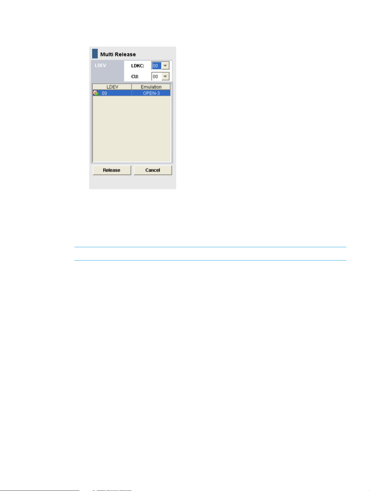
1. Check the Multi Set / Release box, click Release, and then click OK on the confirmation
message.
2. In the Multi Release dialog box, select the desired LDKC and CU image, and select the
desired LDEVs to release from Cache Residency cache.
3. Click Release to return to the Cache Residency window. The requested Cache Residency
operations appear in blue in the LDEV information table.
4. Repeat steps 2 and 3 until all desired operations are listed.
NOTE: The Set is unavailable until you apply (or cancel) your requested operations.
5. Verify the Prestaging setting:
• To enable prestaging, select Prestaging.
• To disable prestaging, clear Prestaging.
6. To start the operations, click Apply:
• If Prestaging was selected, respond to the Yes/No confirmation. To continue with
prestaging, click Yes. To continue without it, click No.
• To cancel the operation, click Cancel and click OK on the confirmation.
7. Monitor the Cache Residency window to make sure that the operations complete successfully.
The cache information area shows the progress of the requested operations.
Changing mode after Cache Residency is registered in cache
If Cache Residency is registered in the cache, the following mode options appear gray and are
unavailable for change:
• Cache Residency Mode (Bind, Priority)
• Prestaging Mode (Yes, No)
To change the mode options:
1. Release the specific data from the Cache Residency cache. For details, see “Releasing specific
data from Cache Residency cache” (page 80).
2. Restore the data with the new settings. For details, see “Placing specific data into Cache
Residency cache” (page 77).
Changing mode after Cache Residency is registered in cache 81
Page 82

13 Troubleshooting
This topic provides references to sources of troubleshooting and contact information for HP Technical
Support.
Troubleshooting resources
For troubleshooting information on the XP P9500, see the HP XP P9000 Owner Guide.
For troubleshooting information on the Remote Web Console software, see the HP XP P9000
Remote Web Console User Guide.
For information on Remote Web Console error codes, see the HP XP P9000 Remote Web Console
Messages.
82 Troubleshooting
Page 83

14 Support and other resources
Contacting HP
For worldwide technical support information, see the HP Support Center:
http://www.hp.com/go/hpsc
Before contacting HP, collect the following information:
• Product model names and numbers
• Technical support registration number (if applicable)
• Product serial numbers
• Error messages
• Operating system type and revision level
• Detailed questions
Subscription service
Receive, by email, support alerts announcing product support communications, driver updates,
software releases, firmware updates, and customer-replaceable component information by signing
up at http://www.hp.com/go/myadvisory.
To change options for support alerts you already receive, click the Sign in link on the right.
Documentation feedback
HP welcomes your feedback.
To make comments and suggestions about product documentation, please send a message to
storagedocsfeedback@hp.com. Include the document title and manufacturing part number. All
submissions become the property of HP.
Related information
The following documents provide related information:
• HP XP P9000 Remote Web Console Messages
• HP XP P9000 Remote Web Console User Guide
You can find these documents on the Manuals page of the HP Business Support Center website:
http://www.hp.com/support/manuals
In the Storage section, click Disk Storage Systems for hardware or Storage Software for software,
and then select your product.
HP websites
For additional information, see the following HP websites:
• http://www.hp.com
• http://www.hp.com/go/storage
• http://www.hp.com/service_locator
• http://www.hp.com/support/manuals
• http://www.hp.com/support/downloads
• http://www.hp.com/storage/whitepapers
Contacting HP 83
Page 84

Conventions for storage capacity values
XP P9000 disk arrays use the following values to calculate physical storage capacity values (hard
disk drives):
• 1 KB (kilobyte) = 1,000 bytes
• 1 MB (megabyte) = 1,0002bytes
• 1 GB (gigabyte) = 1,0003bytes
• 1 TB (terabyte) = 1,0004bytes
• 1 PB (petabyte) = 1,0005bytes
• 1 EB (exabyte) = 1,0006bytes
XP P9000 disk arrays use the following values to calculate logical storage capacity values (logical
devices):
• 1 KB (kilobyte) = 1,024 bytes
• 1 MB (megabyte) = 1,0242bytes
• 1 GB (gigabyte) = 1,0243bytes
• 1 TB (terabyte) = 1,0244bytes
• 1 PB (petabyte) = 1,0245bytes
• 1 EB (exabyte) = 1,0246bytes
Typographic conventions
Table 7 Document conventions
Blue text: Table 7 (page 84)
Bold text
Monospace text
ElementConvention
• Cross-reference links and e-mail addresses
• A cross reference to the glossary definition of the term
in blue text
email addressesBlue, bold, underlined text
Website addressesBlue, underlined text: http://www.hp.com
• Keys that are pressed
• Text typed into a GUI element, such as a box
• GUI elements that are clicked or selected, such as menu
and list items, buttons, tabs, and check boxes
Text emphasisItalic text
• File and directory names
• System output
• Code
• Commands, their arguments, and argument values
Monospace, italic text
WARNING! Indicates that failure to follow directions could result in bodily harm or death.
84 Support and other resources
• Code variables
• Command variables
Emphasized monospace textMonospace, bold text
Page 85

CAUTION: Indicates that failure to follow directions could result in damage to equipment or data.
IMPORTANT: Provides clarifying information or specific instructions.
NOTE: Provides additional information.
TIP: Provides helpful hints and shortcuts.
Typographic conventions 85
Page 86

A Export Tool
This topic explains how to export the monitoring data collected on your storage system into files.
About the Export Tool
Use the Export Tool to export the monitoring data (statistics) shown in the Monitor Performance
window to text files. You can also use the Export Tool to export monitoring data on remote copy
operations performed by Continuous Access Synchronous, Continuous Access Synchronous Z,
Continuous Access Journal, and Continuous Access Journal Z. After exporting monitoring data to
text files, you can import that data into desktop publishing applications, such as Microsoft Word,
or into spreadsheet or database applications for analysis.
Example of a text file
The following example is of a text file imported into spreadsheet software.
NOTE: In this LU_IOPS.csv file, the last four digits of a table column heading (such as 0001
and 0002) indicate a LUN. For example, the heading CL1-A.00(1A-G00).0001 indicates the port
CL1-A, the host group ID 00, the host group name 1A-G00, and the LUN 0001.
If you export monitoring data about concatenated parity groups, the resulting CSV file does not
contain column headings for the concatenated parity groups. For example, if you export monitoring
data about a concatenated parity group named 1-3[1-4], you will be unable to find 1- 3[1-4] in
column headings. To locate monitoring data about 1-3[1-4], find the 1-3 column or the 1-4 column.
Either of these columns contains monitoring data about 1-3[1-4].
Installing the Export Tool
• “System requirements” Page 86
• “Installing the Export Tool on a Windows system” (page 87)
• “Installing the Export Tool on a UNIX system” (page 87)
System requirements
The following components are required to use the Export Tool (for more information, see the HP
P9000 Remote Web Console User Guide):
• A Windows system or a UNIX system
The Export Tool runs on Windows systems and UNIX systems that can run the Remote Web
Console software. If your Windows or UNIX system is unable to run Remote Web Console,
your system is unable to run the Export Tool.
86 Export Tool
Page 87

NOTE: If a firewall exists between the Remote Web Console computer and the SVP, see
Chapter 2 of the HP P9000 Remote Web Console User Guide. In the section “Setting up
TCP/IP for a firewall”, the RMI port numbers listed are the only direct communication settings
required for the Export Tool.
• The Java Runtime Environment (JRE)
To be able to use the Export Tool, you must install Java Runtime Environment on your Windows
or UNIX system. If your system runs Remote Web Console, JRE is already installed on your
system and you can install the Export Tool. If your system does not run Remote Web Console
but contains an appropriate version of JRE, you can install the Export Tool on your system.
The JRE version required for running the Export Tool is the same as the JRE version required
for running Remote Web Console.
• A user ID for exclusive use of the Export Tool
Before you can use the Export Tool, you must create a user ID for exclusive use of the Export
Tool. Assign only the Storage Administrator (Performance Management) role to the user ID
for the Export Tool. It is recommended that you do not assign any roles other than the Storage
Administrator (Performance Management) role to this user ID. The user who is assigned to the
Storage Administrator (Performance Management) role can do the following:
◦ Save the monitoring data into files
◦ Change the gathering interval
◦ Start or stop monitoring by the set subcommand
For details on creating the user ID, see the HP P9000 Remote Web Console User Guide.
• The Export Tool program
CD-ROM Disc 2, which is named Host PP, contains the Export Tool software. For instructions
on installing the Export Tool, see:
◦ “Installing the Export Tool on a Windows system” (page 87)
◦ “Installing the Export Tool on a UNIX system” (page 87)
Installing the Export Tool on a Windows system
The Export Tool program is a Java class file and is located in the export\lib folder.
1. Log on with administrator privileges.
2. Create a new folder for the Export Tool application (for example, C:\Program Files\
monitor). If this folder already exists, skip this step.
3. Insert the Export Tool CD-ROM into the CD drive.
4. Locate the \program\monitor\win_nt folder on the CD-ROM, and copy the self-extracting
file export.exe from the CD-ROM into the new folder you just created.
5. Double-click export.exe to start the installation. The Export Tool is installed, and a new
folder named “export” is created.
Installing the Export Tool on a UNIX system
The Export Tool program is a Java class file and is located in the lib directory.
1. Log on as a superuser.
You do not need to remove a previous installation of Export Tool. The new installation overwrites
the older program.
2. Create a new directory for the Export Tool program (for example, /monitor).
3. Mount the Export Tool CD-ROM.
Installing the Export Tool 87
Page 88

4. Go to the /program/monitor/UNIX directory on the CD-ROM, and copy the export.tar
file to the new directory you just created.
5. Decompress the export.tar file on your system. The Export Tool is installed into the
installation directory.
Using the Export Tool
To be able to export monitoring data, you must first prepare a command file and a batch file, and
then you can run the Export Tool to export monitoring data.
• “Preparing a command file” (page 88)
• “Preparing a batch file” (page 91)
• “Running the Export Tool” (page 92)
Preparing a command file
Before you run the Export Tool, you must write scripts for exporting monitoring data. When writing
scripts, you need to write several subcommands in a command file. When you run the Export Tool,
the subcommands in the command file are executed sequentially, and then the monitoring data is
saved in files.
Example of a command file
svpip 158.214.135.57 ; Specifies IP address of SVP
login expusr passwd ; Logs user into SVP
show ; Outputs storing period to standard
; output
group PhyPG Long ; Specifies type of data to be
; exported and type of
; storing period
group RemoteCopy ; Specifies type of data to be
; exported
short-range 201210010850:201210010910
; Specifies term of data to be
; exported for data stored
; in short range
long-range 201209301430:201210011430
; Specifies term of data to be
; exported for data stored
; in long range
outpath out ; Specifies directory in which files
; will be saved
option compress ; Specifies whether to compress files
apply ; Executes processing for saving
; monitoring data in files
A semicolon (;) indicates the beginning of a comment. Characters from a semicolon to the end of
the line are comments.
The scripts in this command file are explained as follows:
• svpip 158.214.135.57
• login expusr passwd
88 Export Tool
This script specifies that you are logging into SVP whose IP address is 158.214.135.57.
You must log into SVP when using the Export Tool.
The svpip subcommand specifies the IP address of SVP. You must include the svpip
subcommand in your command file. For detailed information about the svpip subcommand,
see “svpip” (page 96).
This script specifies that you use the user ID expusr and the password passwd to log into
SVP.
Page 89

The login subcommand logs the specified user into SVP. You must include the login
subcommand in your command file. For detailed information about the login subcommand,
see “login” (page 98).
CAUTION: When you write the login subcommand in your command file, you must specify
a user ID that should be used exclusively for running the Export Tool. See “System requirements”
(page 86) for reference.
• show
The show subcommand checks SVP to find the period of monitoring data stored in SVP and
the data collection interval (called gathering interval in Performance Monitor), and then outputs
them to the standard output (for example, the command prompt) and the log file.
Performance Monitor collects statistics by the two types of storing periods: in short range and
in long range. The show subcommand displays the storing periods and the gathering intervals
for these two types of monitoring data.
The following is an example of information that the show subcommand outputs:
Short Range From: 2012/10/01 01:00 - To: 2012/10/01 15:00 Interval:
1min. Long Range From: 2012/09/01 00:00 - To: 2012/10/01 15:00
Interval: 15min.
Short Range indicates the storing period and gathering interval of the monitoring data
stored in short range. Long Range indicates those of the monitoring data stored in long
range. In the above example, the monitoring data in short range is stored every 1 minute in
the term of 1:00-15:00 on Oct. 1, 2012. Also, the monitoring data in long range is stored
every 15 minutes in the term of Sep. 1, 2012, 0:00 through Oct. 1, 2012, 15:00. When
you run the Export Tool, you can export monitoring data within these periods into files.
All the monitoring items are stored in short range, but a part of monitoring items is stored in
both the short range and long range. For details on monitoring items that can be stored in
long range, see “long-range” (page 111).
The use of the show subcommand is not mandatory, but it is recommended that you include
the show subcommand in your command file. If an error occurs when you run the Export Tool,
you might be able to find the error cause by checking the log file for information issued by
the show subcommand. For detailed information about the show subcommand, see “show”
(page 98).
• group PhyPG Long and group RemoteCopy
The group subcommand specifies the type of data that you want to export. Specify a operand
following group to define the type of data to be exported. Basically, monitoring data stored
in short range is exported. But you can direct to export monitoring data stored in long range
when you specify some of the operands.
The example script group PhyPG Long in “Preparing a command file” (page 88) specifies
to export usage statistics about parity groups in long range. Also, the script
group RemoteCopy specifies to export statistics about remote copy operations by Continuous
Access Synchronous and Continuous Access Synchronous Z in short range. You can describe
multiple lines of the group subcommand to export multiple monitoring items at the same time.
For detailed information about the group subcommand, see “group” (page 99).
• short-range 201210010850:201210010910 and long-range
201209301430:201210011430
The short-range and long-range subcommands specify the term of monitoring data to
be exported. Use these subcommands when you want to narrow the export-target term within
Using the Export Tool 89
Page 90

the stored data. You can specify both the short-range and long-range subcommands
at the same time. The difference between these subcommands is as follows:
◦ The short-range subcommand is valid for monitoring data in short range. You can
use this subcommand to narrow the export-target term for all the monitoring items you
can specify by the group subcommand.
Specify a term within "Short Range From XXX To XXX" which is output by the show
subcommand.
◦ The long-range subcommand is valid for monitoring data in long range. You can use
this subcommand only when you specify the PhyPG, PhyLDEV, PhyProc, or PhyESW
operand with the Long option in the group subcommand. (The items that can be saved
by these operands are the monitoring data displayed in the Physical tab of the Performance
Management window with selecting longrange.)
Specify a term within "Long Range From XXX To XXX" which is output by the show
subcommand.
In the sample file in “Preparing a command file” (page 88), the script short-range
201210010850:201210010910 specifies the term 8:50-9:10 on Oct. 1, 2012. This script
is applied to the group RemoteCopy subcommand in this example. When you run the
Export Tool, it will export the statistics about remote copy operations by Continuous Access
Synchronous and Continuous Access Synchronous Z in the term specified by the short-range
subcommand.
Also, in “Preparing a command file” (page 88), the script long-range
201209301430:201210011430 specifies the term from Sep. 30, 2012, 14:30 to Oct. 1,
2012, 14:30. This script is applied to the group PhyPG Long subcommand in this example.
When you run the Export Tool, it will export the usage statistics about parity groups in the
term specified by the long-range subcommand.
If you run the Export Tool without specifying the short-range or long-range subcommand,
the monitoring data in the whole storing period (data in the period displayed by the show
subcommand) will be exported.
◦ For detailed information about the short-range subcommand, see “Short-range”
(page 109).
◦ For detailed information about the long-range subcommand, see “long-range”
(page 111).
• outpath out
This script specifies that files should be saved in the directory named out in the current
directory.
The outpath subcommand specifies the directory in which files should be saved. For detailed
information about the outpath subcommand, see “outpath” (page 113).
• option compress
This script specifies that the Export Tool should compress monitoring data in ZIP files.
The option subcommand specifies whether to save files in ZIP format or in CSV format. For
detailed information about the option subcommand, see “option” (page 113).
• apply
The apply subcommand saves monitoring data in files. For detailed information about the
apply command, see “apply” (page 114).
When you install the Export Tool, the command.txt file is stored in the installation directory. This
file contains sample scripts for your command file. It is recommended that you customize scripts
in command.txt according to your needs. For details about subcommand syntax, see “Export
Tool command reference” (page 95).
90 Export Tool
Page 91

Preparing a batch file
A batch file is used to run the Export Tool. The Export Tool starts and saves monitoring data in files
when you execute the batch file.
The installation directory for the Export Tool contains two default batch files: runWin.bat for
Windows systems, and runUnix.bat for UNIX systems.
The following examples illustrate scripts in the runWin.bat and runUnix.bat batch files. These
batch files include a command line that executes a Java command. When you execute the batch
file, the Java command executes the subcommands specified in the command file and then saves
monitoring data in files.
Example batch file for Windows systems (runWin.bat):
java -classpath
"./lib/JSanExport.jar;./lib/JSanRmiApiEx.jar;./lib/JSanRmiServerUx.jar"
-Xmx536870912 -Dmd.command=command.txt -Dmd.logpath=log
sanproject.getmondat.RJMdMain<CR+LF> pause<CR+LF>
Example batch file for UNIX systems (runUnix.bat):
#! /bin/sh<LF> java -classpath
"./lib/JSanExport.jar:./lib/JSanRmiApiEx.jar:./lib/JSanRmiServerUx.jar"
-Xmx536870912 -Dmd.command=command.txt -Dmd.logpath=log
sanproject.getmondat.RJMdMain<LF>
In the previous scripts, <CR+LF> and <LF> indicate the end of a command line.
If the system running the Export Tool communicates directly with SVP, you usually do not need to
change scripts in runWin.bat and runUnix.bat. However, you might need to edit the Java
command script in a text editor in some cases, for example:
• if the name of your command file is not command.txt
• if you moved your command file to a different directory
• if you do not want to save in the log directory
• if you want to name log files as you like
If the system that runs the Export Tool communicates with SVP via a proxy host, edit the Java
command script in a text editor. to specify the host name (or the IP address) and the port number
of the proxy host. For example, if the host name is Jupiter and the port number is 8080, the resulting
command script would be as shown in the following examples:
Example of specifying a proxy host on Windows (runWin.bat):
java -classpath
"./lib/JSanExport.jar;./lib/JSanRmiApiEx.jar;./lib/JSanRmiServerUx.jar"
-Dhttp.proxyHost=Jupiter -Dhttp.proxyPort=8080 -Xmx536870912
-Dmd.command=command.txt -Dmd.logpath=log sanproject.getmondat.RJMdMain
<CR+LF> pause <CR+LF>
Example of specifying a proxy host on UNIX (runUnix.bat):
#! /bin/sh <LF> java -classpath
"./lib/JSanExport.jar:./lib/JSanRmiApiEx.jar:./lib/JSanRmiServerUx.jar"
-Dhttp.proxyHost=Jupiter -Dhttp.proxyPort=8080 -Xmx536870912
-Dmd.command=command.txt -Dmd.logpath=log sanproject.getmondat.RJMdMain
<LF>
In the preceding scripts, <CR+LF> and <LF> indicates the end of a command line.
If the IP address of the proxy host is 158.211.122.124 and the port number is 8080, the resulting
command script is as follows:
Example batch file for Windows systems (runWin.bat):
java -classpath
"./lib/JSanExport.jar;./lib/JSanRmiApiEx.jar;./lib/JSanRmiServerUx.jar"
-Dhttp.proxyHost=158.211.122.124 -Dhttp.proxyPort=8080 -Xmx536870912
Using the Export Tool 91
Page 92

-Dmd.command=command.txt -Dmd.logpath=log sanproject.getmondat.RJMdMain
<CR+LF> pause <CR+LF>
Example batch file for UNIX systems (runUnix.bat):
#! /bin/sh <LF> java -classpath
"./lib/JSanExport.jar:./lib/JSanRmiApiEx.jar:./lib/JSanRmiServerUx.jar"
-Dhttp.proxyHost=158.211.122.124 -Dhttp.proxyPort=8080 -Xmx536870912
-Dmd.command=command.txt -Dmd.logpath=log sanproject.getmondat.RJMdMain
<LF>
In the above scripts, <CR+LF> and <LF> indicates the end of a command line.
For detailed information about syntax of the Java command, see “Java” (page 116).
Running the Export Tool
CAUTION: Running multiple instances of the Export Tool simultaneously is not supported. If you
run multiple instances, the SVP might become overloaded and a timeout error might occur.
To save monitoring data in files, launch the Export Tool by running the batch file:
From a system running UNIX, enter the name of the batch file at the command prompt, and then
press the <Enter> key.
From a system running Windows, double-click the batch file to run it.
c:\WINDOWS> cd c:\export
c:\export> runWin.bat
Dots (...) appear on the screen until the system finishes exporting data. If an internal error occurs,
an exclamation mark (!) appears, and then the Export Tool restarts automatically.
Example of command prompt outputs from the Export Tool:
[ 2] svpip 158.214.135.57
[ 3] login User = expusr, Passwd = [****************]
:
:
[ 6] group Port
:
:
[20] apply
Start gathering port data
Target = 16, Total = 16
+----+----+----+----+----+----+----+----+----+----+
...........................!
.................................
End gathering port data
By default, the system compresses monitoring data files into a ZIP-format archive file. When you
want to view the monitoring data, you can decompress and extract the CSV files from the ZIP
archive. If your system is not able to extract files from a ZIP archive, you need to obtain software
to view the data.
NOTE: You can change the default method of exporting files to an uncompressed format. However,
the resulting files could be significantly larger and take longer to compile. For more information,
see option Subcommand “option” (page 113).
For a complete list of files to be saved by the Export Tool, see “Using the Export Tool” (page 88).
File formats
If you specify the nocompress operand for the option subcommand, the Export Tool saves files
in CSV format instead of ZIP format (For detailed information, see option Subcommand “option”
(page 113)). When files are saved in CSV format instead of ZIP format, the file saving process could
take longer and the resulting files could be larger.
92 Export Tool
Page 93

Processing time
Files saved by the Export Tool are often very large. The total file size for all the files can be as
large as approximately 2 GB. For this reason, the exporting process might take a lot of time. If
you want to export statistics spanning a long period of time, it is recommended that you run the
Export Tool multiple times for different periods, rather than run it one time to export the entire time
span as a single large file. For example, if you want to export statistics spanning 24 hours, run
the tool eight times to export statistics in three 3- hour increments.
The next table provides lists time estimates for exporting monitoring data files using different
operands in the group subcommand:
Table 8 Estimate of time required for exporting files
subcommand
RemarksEstimated timeOperand for the group
5 minutesPort
5 minutesPortWWN
This estimate assumes that the Export Tool should save statistics about
128 ports within a 24-hour period.
This estimate assumes that the Export Tool should save statistics about
128 ports within a 24-hour period.
This estimate assumes that:60 minutesLDEV
• The Export Tool should save statistics about 8,192 volumes within a
24-hour period.
• The Export Tool is used eight times. Each time the Export Tool is used,
the tool obtains statistics within a 3-hour period.
This estimate assumes that:60 minutesLU
• The Export Tool should save statistics about 12,288 LUs within a
24-hour period.
• The Export Tool is used eight times. Each time the Export Tool is used,
the tool obtains statistics within a 3-hour period.
NOTE:
• The estimated time in the table is for the 1-minute interval of data collection. If the interval is
2 minutes, "a 24-hour period" in the table will be "a 48-hour period", because the interval
is proportional to the stored time.
• The estimated time that includes the transfer time of the network might take a lot of time
depending on the transmission speed of the network.
• To shorten the acquisition time, specify the option of the group command to narrow acquisition
objects. For details about the group command, see “group” (page 99).
Termination code
If you want to use a reference to a termination code in your batch file, do the following:
• To use such a reference in a Windows batch file, write %errorlevel% in the batch file.
• To use such a reference in a UNIX Bourne shell script, write $? in the shell script.
• To use such a reference in a UNIX C shell script, write $status in the shell script.
A reference to a termination code is used in the following example of a Windows batch file. If this
batch file executes and the Export Tool returns the termination code 1 or 3, the command prompt
displays a message that indicates the set subcommand fails.
java -classpath
"./lib/JSanExport.jar;./lib/JSanRmiApiEx.jar;./lib/JSanRmiServerUx.jar"
-Xmx536870912 -Dmd.command=command.txt -Dmd.logpath=log
sanproject.getmondat.RJMdMain<CR+LF> if %errorlevel%==1 echo THE SET
SUBCOMMAND FAILED<CR+LF> if %errorlevel%==3 echo THE SET SUBCOMMAND
FAILED<CR+LF> pause<CR+LF>
Using the Export Tool 93
Page 94

Log files
In the previous scripts, <CR+LF> indicates the end of a command line.
When the Export Tool runs, the Export Tool creates a new log file on your system. Therefore, if
you run the Export Tool repeatedly, the size of free space on your system will be reduced. To secure
free space on your system, you are strongly recommended to delete the Export Tool log files
regularly. For details about the location of the log files, see “Java” (page 116).
The Export Tool returns a termination code when the Export Tool finishes.
Table 9 Termination codes returned by the export tool
MeaningTermination
code
The Export Tool finished successfully.0
1
3
Error handling
When an internal error occurs during export processing, an exclamation mark (!) appears to signal
an error. By default, the Export Tool makes up to three more attempts at processing. You can
change the maximum number of retries by using the retry subcommand. For detailed information
about the retry subcommand, see “retry” (page 97).
If export processing does not finish within three retries or if an internal error occurs other than those
listed in the following table, the Export Tool stops. If the Export Tool stops, quit the command
prompt, and then run the tool again.
For more information, see “Troubleshooting the Export Tool” (page 133).
Errors for which export tool retries processing
An error occurred when the set subcommand (see “set” (page 114)) executed, because an attempt
to switch to Modify mode failed. Some other user might have been logged on in Modify mode.
One of the following two errors occurred;2
• A command file has been corrupted or could not be read.
• An error occurred when a command was parsed.
An error occurred due to more than one reason. One of the reasons is that an attempt to switch to
Modify mode failed when the set subcommand (see “set” (page 114)) executed. Some other user
might have been logged on in Modify mode.
The Storage Administrator (Performance Management) role is not assigned to the user ID.4
94 Export Tool
Cause of errorError message ID
An error occurred during SVP processing.0001 4001
Because SVP is busy, the monitoring data cannot be obtained.0001 5400
An administrator is changing a system environment file.0001 5508
Array is refreshing, or the settings by the user are registered.0002 2016
The storage system is in internal process, or some other user is changing configuration.0002 5510
Now processing.0002 6502
Another user has lock.0002 9000
A service engineer is accessing the storage system in Modify mode.0003 2016
SVP is not ready yet, or an internal processing is being executed.0003 2033
An error occurred during SVP processing.0003 3006
The storage system status is invalid.0405 8003
Page 95

Cause of errorError message ID
An internal process is being executed, or maintenance is in progress.5205 2003
SVP is now updating the statistics data.5205 2033
SVP is now updating the statistics data.5305 2033
The storage system status is invalid.5305 8002
Export Tool command reference
This topic provides the syntax of the Export Tool subcommands that you can write in your command
file and the command that should be used in your batch file. “Subcommand list” (page 96) lists
the subcommands explained in this topic. The Java command is explained in “Java” (page 116).
Export Tool command syntax
This topic explains the syntax of Export tool subcommands that you can write in your command
file. This topic also explains the syntax of the Java command that should be used in your batch
file.
Conventions
The following conventions are used to explain syntax:
DescriptionConvention
italics
{ }
Syntax descriptions
Indicates characters that you must type exactly as they are shown.bold
Indicates a type of an operand. You do not need to type characters in italics exactly as they are
shown.
Indicates one or more operands that can be omitted.[ ]
If two or more operands are enclosed by these square brackets and are delimited by vertical bars
(|), you can select one of the operands.
Indicates that you must select one operand from the operands enclosed by the braces. Two or
more operands are enclosed by the braces and are delimited by vertical bars (|).
Indicates that a previously used operand can be repeated....
Vertical bar delimiter, indicating you can select one of the operands enclosed in square brackets.|
Indicates you can write this script...This syntax...
connect 123.01.22.33connect ip-address
destinationdestination [directory]
destination c:\temp
compresscompress [yes|no]
compress yes
compress no
answer yesanswer {yes|no}
answer no
portsports [name][...]
ports port-1
ports port-1 port-2
Export Tool command reference 95
Page 96

Writing a script in the command file
When you write a script in your command file, be aware of the following:
• Ensure that only one subcommand is used in one line.
• Empty lines in any command file will be ignored.
• Use a semicolon (;) if you want to insert a comment in your command file. If you enter a
semicolon in one line, the remaining characters in that line will be regarded as a comment.
Following are examples of comments in a command file:
;;;;;;; ;;;;;;;;;;;;;;;;;;;;;;;;;;;;;;;;
;;; COMMAND FILE: command.txt ;;;;
;;;;;;;;;; ;;;;;;;;;;;;;;;;;;;;;;;;;;;;;
svpip 158.214.135.57 ; IP address of SVP
login expusr "passwd" ; Log onto SVP
Viewing the online Help for subcommands
You can display the online Help to view the syntax of subcommands when you are working at the
command prompt. To be able to view the online Help, you must use the help subcommand of the
Export Tool. For more information about how to use the help subcommand, see “help” (page 115).
Subcommand list
FunctionSubcommand
“show” (page 98)
“Short-range” (page 109)
“long-range” (page 111)
“set” (page 114)
Specifies the IP address of SVP to be logged in.“svpip” (page 96)
Makes settings on retries of export processing.“retry” (page 97)
Logs the specified user into SVP.“login” (page 98)
Checks SVP to find the period of monitoring data stored in SVP and the data
collection interval (that is called “gathering interval”), and then outputs them to
the standard output and the log file.
Specifies the type of data that you want to export.“group” (page 99)
Specifies the term of monitoring data to be exported for short-range monitoring
data.
Specifies the term of monitoring data to be exported for long-range monitoring
data.
Specifies the directory in which files should be saved.“outpath” (page 113)
Specifies whether to save files in ZIP format or in CSV format.“option” (page 113)
Saves monitoring data in files.“apply” (page 114)
Starts or ends monitoring of the storage system, and specifies the gathering
interval in short-range monitoring.
Displays the online help for subcommands.“help” (page 115)
Starts the Export tool and writes monitoring data into files.“Java” (page 116)
svpip
Description
This subcommand specifies the IP address or the host name of SVP.
Syntax
svpip {ip-address|host-name}
96 Export Tool
Page 97

retry
Operands
DescriptionOperand
Specifies the IP address of SVP.ip-address
If SVP is managed with IPv6 (Internet Protocol Version 6), you must specify the ip-address operand
to match the format of IPv6. If the Export Tool runs on Windows XP, the interface identifier (for
example, "%5") must be added to the end of the specified IP address.
Specifies the host name of SVP.host-name
Alphanumeric characters, hyphen, and period can be specified. Underscore (_) cannot be
specified. The host name can include a hyphen but must be enclosed by double quotation marks
(").
Example
The following example specifies the IP address of SVP as 158.214.127.170.
svpip 158.214.127.170
Description
This subcommand makes settings on retries of export processing.
When an internal error occurs during export processing, the Export Tool stops processing and then
retries export processing. By default, the Export Tool can retry processing up to three times, but
you can change the maximum number of retries by using the retry subcommand.
By default, the interval between one retry and the next retry is two minutes. You can change the
interval by using the retry subcommand.
The retry subcommand must execute before the login subcommand executes.
Syntax
retry [time=m] [count=n]
Operands
DescriptionOperand
time=m
Specifies the interval between retries in minutes, where m is a value within the range of 1 to
59.
If this operand is omitted, the interval between retries is two minutes.
Specifies the maximum number of retries.count=n
If n is 0, the number of retries is unlimited.
If this operand is omitted, the maximum number of retries is 3.
Example
If the following command file is used, the interval between retries is 5 minutes and the maximum
number of retries is 10.
svpip 158.214.135.57 retry time=5 count=10login expusr passwd
show group Portshort-range 201204010850:201204010910outpath
outoption compressapply
Export Tool command reference 97
Page 98
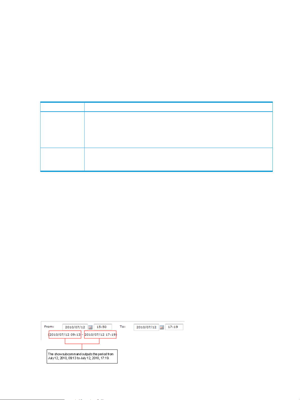
login
Description
This e subcommand uses a user ID and a password to log the specified user in SVP.
The svpip subcommand must execute before the login subcommand executes.
The login subcommand fails if monitoring data does not exist in SVP.
Syntax
login userid password
Operands
DescriptionOperand
Specifies the user ID for SVP.userid
If the user ID includes any non-alphanumeric character, the user ID must be enclosed by double
quotation marks (").
Be sure to specify a user ID that should be used exclusively with the Export Tool. For detailed
information, see “System requirements” (page 86).
Specifies the password of the user.password
If the password includes any non-alphanumeric character, the password ID must be enclosed
by double quotation marks (").
show
Example
This example logs the user expusr into SVP whose IP address is 158.214.127.170. The password
is pswd.
svpip 158.214.127.170 login expuser pswd
Description
This subcommand outputs the following information to the standard output (for example, to the
command prompt):
• the period during which monitoring data was collected onto SVP (storing period)
• the interval at which the monitoring data was collected (gathering interval)
Performance Monitor collects statistics by the two types of storing periods: in short range and in
long range. In short-range monitoring, the monitoring data between 8 hours and 15 days is stored
in SVP, and in long-range monitoring, the monitoring data up to 3 months is stored in SVP. For
details on the two storing periods, see “Short-range” (page 109) and “long-range” (page 111).
Storing periods output by the show subcommand are the same as the information displayed in the
Monitoring Term area of the Monitor Performance window.
Figure 19 The monitoring term area
The login command must execute before the show subcommand executes.
98 Export Tool
Page 99

group
Syntax
show
Outputs
The show subcommand displays the storing period and the gathering interval for these two types
of monitoring data: in short range and in long range. For example, the show subcommand outputs
the following information:
Short Range From: 2012/10/01 01:00 - To: 2012/10/01 15:00 Interval:
1min. Long Range From: 2012/09/01 00:00 - To: 2012/10/01 15:00 Interval:
15min.
Short Range indicates the storing period and gathering interval of the monitoring data stored
in short range. Long Range indicates those of the monitoring data stored in long range. When
you run the Export Tool, you can export the monitoring data within these periods into files. If you
use the short-range or long-range subcommand additionally, you can narrow the term of
data to be exported (see “Short-range” (page 109) or “long-range” (page 111)).
From indicates the starting time for collecting monitoring data. To indicates the ending time for
collecting monitoring data.
Interval indicates the interval at which the monitoring data was collected (gathering interval).
For example, Interval 15min. indicates that monitoring data was collected at 15-minute
intervals.
Description
The group subcommand specifies the type of monitoring data that you want to export. This
command uses an operand (for example, PhyPG and PhyLDEV above) to specify a type of
monitoring data.
Table 10 (page 100) shows the monitoring data that can be saved into files by each operand, and
the saved ZIP files. For details on the monitoring data saved in these files, see the tables listed in
the See column.
Export Tool command reference 99
Page 100

Table 10 Operands of the group subcommand and saved monitoring data
PhyPG
PhyLDEV
PhyExG
PhyExLDEV
PhyProc
PhyESW
GUI operationOperand
Select Parity Groups
from Object list in
Performance Objects
field in Monitor
Performance window.
Select Logical Device
from Object list in
Performance Objects
field in Monitor
Performance window.
Select Controller from
Object list in
Performance Objects
field in Monitor
Performance window.
Select Access Path from
Object list in
Performance Objects
field in Monitor
Performance window.
the file
Usage statistics about
parity groups
Usage statistics about
volumes
external volume groups
Usage conditions about
external volumes
Usage statistics about MPs
and data recovery and
reconstruction processors
Usage statistics about
access paths, write
pending rate, and cache
PhyPG_dat.ZIP
PhyLDEV_dat.ZIP
1
1
PhyExG_dat.ZIPUsage conditions about
PhyExLDEV_dat/PHY_ExLDEV_XXXXX.ZIP
2
PhyProc_dat.ZIP
PhyESW_dat.ZIP
1
1
SeeSaved ZIP fileMonitoring data saved in
Table 12 (page
118)
PG
LDEV
Port
PortWWN
LU
PPCGWWN
Select Parity Group
from Object list in
Performance Objects
field in Monitor
Performance window.
Select Logical Device
from Object list in
Performance Objects
field in Monitor
Performance window.
list in Performance
Objects field in Monitor
Performance window.
Select WWN from
Object list in
Performance Objects
field in Monitor
Performance window.
list in Performance
Objects field in Monitor
Performance window.
Select WWN from
Object list in
Performance Objects
field in Monitor
Performance window.
groups, external volume
groups, or V-VOL groups
Statistics about volumes in
parity groups, in external
volume groups, or in V-VOL
groups
adapters connected to
ports
are connected to ports
PG_dat.ZIPStatistics about parity
LDEV_dat/LDEV_XXXXX.ZIP
Port_dat.ZIPStatistics about portsSelect Port from Object
PortWWN_dat.ZIPStatistics about host bus
LU_dat.ZIPStatistics about LUsSelect LUN from Object
PPCGWWN_dat.ZIPAll host bus adapters that
Table 13 (page
121)
3
Table 14 (page
122)
Table 16 (page
125)
Table 17 (page
125)
Table 18 (page
125)
Table 19 (page
126)
RemoteCopy
100 Export Tool
Usage Monitor tab in
the Continuous Access
copy operations by
Continuous AccessSynchronous and
Synchronous and
RemoteCopy_dat.ZIPStatistics about remote
Table 21 (page
127)
 Loading...