HP e4401b, 252c02b, 252c03b, 252c04b, 252c05b schematic

...

Download

Measurement Guide and Programming

Examples

PSA and ESA Series Spectrum Analyzers

This manual provides documentation for the following instruments:

Agilent Technologies PSA Series

E4443A (3 Hz - 6.7 GHz) E4445A (3 Hz - 13.2 GHz) E4440A (3 Hz - 26.5 GHz)

E4446A (3 Hz - 44 GHz)

E4448A (3 Hz - 50 GHz)

Agilent Technologies ESA-E Series

E4401B (9 kHz - 1.5 GHz) E4402B (9 kHz - 3.0 GHz) E4404B (9 kHz - 6.7 GHz)

E4405B (9 kHz - 13.2 GHz)

E4407B (9 kHz - 26.5 GHz)

Agilent Technologies ESA-L Series

E4411B (9 kHz - 1.5 GHz) E4403B (9 kHz - 3.0 GHz)

E4408B (9 kHz - 26.5 GHz)

Manufacturing Part Number: E4401-90482

Supersedes: E4401-90466

Printed in USA

April 2004

Notice

The information contained in this document is subject to change without notice.

Agilent T echnologies makes no war ranty of any kind with r egard to this material, including but not limited to, the implied warranties of merchantability and fitness for a partic ular purpose. Agilent Technologies shall not be liable for errors contained herein or for incidental or consequential damages in connection with the furnishing, performance, or use of this material.

Safety Information

The following safety symbols are used throughout this manual. Familiarize yourself with the symbols and their meaning before operating this instrument.

WARNING Warning denotes a hazard. It calls attention to a procedure

which, if not correctly performed or adhered to, could result in injury or loss of life. Do not proceed beyond a warning note until the indicated conditions are fully understood and met.

CAUTION Caution denotes a hazard. It calls attention to a procedure that, if not

correctly performed or adhered to, could result in dam a g e to or destruction of the instrument. Do not proceed beyond a caution sign until the indicated conditions are fully understood and met.

NOTE Note calls out special information for the user’s attention. It provides

operational information or additional instructions of which the user should be aware.

The instruction documentation symbol. The product is

marked with this symbol when it is necessary for the user to refe r to th e instructions in the docu mentation .

This symbol is used to mark the on position of the

power line switch.

This symbol is used to mark the s tandby p osit ion o f the

power line switch.

This symbol indicates that the input power required is

AC.

WARNING This is a Safety Class 1 Product (provided with a protective

earth ground incorporated in the power cord). The mains plug shall be inserted only in a socket outlet provided with a protected earth contact. Any interruption of the protective conductor inside or outside of the product is likely to make the product dangerous. Intentional interruption i s prohib ited.

WARNING No operator serviceable parts inside. Refer servicing to

qualified personnel. To prevent electrical shock do not remove covers.

WARNING If this product is not used as specified, the protection provided

by the equipment could be impaired. This product must be used in a normal condition (in which all means for protection are intact) only.

CAUTION Always use the three-prong AC power cord supplied with this product.

Failure to ensure adequate grounding may cause product damage.

Where to Find the Latest Information

Documentation is updated periodically. Fo r the latest information about Agilent Technologies PSA and ESA spectrum analyzers, including firmware upgrades and application information, please visit the following Internet URL:

http://www .agilent.com/find/psa http://www.agilent.com/find/esa

Microsoft is a U.S. registered trademark of Microsoft Corporation.

Bluetooth is a trademark owned by its proprietor and used under license.

Contents

1. Recommended Test Equipment

2. Measuring Multiple Signals

Comparing Signals on the Same Screen Using Marker Delta . . . . . . . . . . . . . . . . . . . . . . . 12

Comparing Signals on the Same Screen Using Marker Delta Pair . . . . . . . . . . . . . . . . . . . . 14

Comparing Signals not on the Same Screen Using Marker Delta . . . . . . . . . . . . . . . . . . . . 15

Resolving Signals of Equal Amplitude . . . . . . . . . . . . . . . . . . . . . . . . . . . . . . . . . . . . . . . . . 17

Resolving Small Signals Hidden by Large Signals . . . . . . . . . . . . . . . . . . . . . . . . . . . . . . . 20

Decreasing the Frequency Span Around the Signal . . . . . . . . . . . . . . . . . . . . . . . . . . . . . . . 22

3. Measuring a Low−Level Signal

Reducing Input Attenuation . . . . . . . . . . . . . . . . . . . . . . . . . . . . . . . . . . . . . . . . . . . . . . . . . 26

Decreasing the Resolution Bandwidth . . . . . . . . . . . . . . . . . . . . . . . . . . . . . . . . . . . . . . . . . 28

Using the Average Detector and Increased Sweep Time . . . . . . . . . . . . . . . . . . . . . . . . . . . 29

Trace Averaging . . . . . . . . . . . . . . . . . . . . . . . . . . . . . . . . . . . . . . . . . . . . . . . . . . . . . . . . . . 30

4. Improving Frequency Resolution and Accuracy

Using a Frequency Counter to Improve Frequency Resolution and Accuracy . . . . . . . . . . 32

5. Tracking Drifting Signals

Measuring a Source’s Frequency Drift . . . . . . . . . . . . . . . . . . . . . . . . . . . . . . . . . . . . . . . . . 36

Tracking a Signal . . . . . . . . . . . . . . . . . . . . . . . . . . . . . . . . . . . . . . . . . . . . . . . . . . . . . . . . . 38

6. Making Distortion Measurements

Identifying Analyzer Generated Distortion . . . . . . . . . . . . . . . . . . . . . . . . . . . . . . . . . . . . . 40

Third-Order Intermodulation Distortion . . . . . . . . . . . . . . . . . . . . . . . . . . . . . . . . . . . . . . . . 42

Measuring TOI Distortion with a One-Button Measurement . . . . . . . . . . . . . . . . . . . . . . . . 44

Measuring Harmonics and Harmonic Distortion with a One-Button Measurement . . . . . . 45

7. Measuring Noise

Measuring Signal-to-Noise . . . . . . . . . . . . . . . . . . . . . . . . . . . . . . . . . . . . . . . . . . . . . . . . . . 48

Measuring Noise Using the Noise Marker . . . . . . . . . . . . . . . . . . . . . . . . . . . . . . . . . . . . . . 50

Measuring Noise-Like Signals Using Marker Pairs . . . . . . . . . . . . . . . . . . . . . . . . . . . . . . . 52

Measuring Noise-Like Signals Using the Channel Power Measurement . . . . . . . . . . . . . . . 54

8. Making Time-Gated Measurements

Generating a Pulsed-RF FM Signal . . . . . . . . . . . . . . . . . . . . . . . . . . . . . . . . . . . . . . . . . . . 58

Connecting the Instruments to Make Time-Gated Measurements . . . . . . . . . . . . . . . . . . . . 61

Gated LO Measurement (PSA) . . . . . . . . . . . . . . . . . . . . . . . . . . . . . . . . . . . . . . . . . . . . . . . 62

Gated Video Measurement (ESA) . . . . . . . . . . . . . . . . . . . . . . . . . . . . . . . . . . . . . . . . . . . . 64

Gated FFT Measurement (PSA) . . . . . . . . . . . . . . . . . . . . . . . . . . . . . . . . . . . . . . . . . . . . . . 66

Contents

Table of Contents

9. Measuring Digital Communications Signals

Making Burst Power Measurements . . . . . . . . . . . . . . . . . . . . . . . . . . . . . . . . . . . . . . . . . . .68

Making Statistical Power Measurements (CCDF) . . . . . . . . . . . . . . . . . . . . . . . . . . . . . . . . .71

Making Adjacent Channel Power (ACP) Measurements . . . . . . . . . . . . . . . . . . . . . . . . . . .74

Making Multi-Carrier Power (MCP) Measurements . . . . . . . . . . . . . . . . . . . . . . . . . . . . . . .77

10.Using External Millimeter Mixers (Option AYZ)

Making Measurements With Agilent 11970 Series Harmonic Mixers . . . . . . . . . . . . . . . . .82

Setting Harmonic Mixer Bias Current . . . . . . . . . . . . . . . . . . . . . . . . . . . . . . . . . . . . . . . . . .84

Entering Conversion-Loss Correction Data for Harmonic Mixers . . . . . . . . . . . . . . . . . . . .85

Making Measurements with Agilent 11974 Series Preselected Harmonic Mixers . . . . . . . .86

Frequency Tracking Calibration with Agilent 11974 Series Preselected Harmonic Mixers .88

11.Demodulating AM and FM Signals

Measuring the Modulation Rate of an AM Signal . . . . . . . . . . . . . . . . . . . . . . . . . . . . . . . . .92

Measuring the Modulation Index of an AM Signal . . . . . . . . . . . . . . . . . . . . . . . . . . . . . . . .94

Demodulating an AM Signal Using the ESA Series . . . . . . . . . . . . . . . . . . . . . . . . . . . . . . .96

Demodulating an FM Signal Using the ESA-E Series (Requires Option BAA) . . . . . . . . . .98

12.Using Segmented Sweep (ESA-E Series Spectrum Analyzers)

Measuring Harmonics Using Standard Sweep . . . . . . . . . . . . . . . . . . . . . . . . . . . . . . . . . .102

Measuring Harmonics Using Segmented Sweep . . . . . . . . . . . . . . . . . . . . . . . . . . . . . . . . .104

Using Segmented Sweep With Limit Lines . . . . . . . . . . . . . . . . . . . . . . . . . . . . . . . . . . . . .106

Using Segmented Sweep to Monitor the Cellular Activity of a cdmaOne Band . . . . . . . .108

13.Stimulus Response Measurements (ESA Options 1DN and 1DQ)

Making a Stimulus Response Transmission Measurement . . . . . . . . . . . . . . . . . . . . . . . . .112

Calculating the N dB Bandwidth Using Stimulus Response . . . . . . . . . . . . . . . . . . . . . . . .114

Measuring Stop Band Attenuation Using Log Sweep (ESA-E Series) . . . . . . . . . . . . . . . .116

Making a Reflection Calibration Measurement . . . . . . . . . . . . . . . . . . . . . . . . . . . . . . . . . .118

Measuring Return Loss using the Reflection Calibration Routine . . . . . . . . . . . . . . . . . . .120

14.Demodulating and Viewing Television Signals (ESA-E Series Option B7B)

Demodulating and Viewing Television Signals . . . . . . . . . . . . . . . . . . . . . . . . . . . . . . . . .122

Measuring Depth of Modulation . . . . . . . . . . . . . . . . . . . . . . . . . . . . . . . . . . . . . . . . . . . . .126

15.Concepts

Resolving Closely Spaced Signals . . . . . . . . . . . . . . . . . . . . . . . . . . . . . . . . . . . . . . . . . . . .130

Harmonic Distortion Calculations . . . . . . . . . . . . . . . . . . . . . . . . . . . . . . . . . . . . . . . . . . . .132

Time Gating Concepts . . . . . . . . . . . . . . . . . . . . . . . . . . . . . . . . . . . . . . . . . . . . . . . . . . . . .133

Trigger Concepts . . . . . . . . . . . . . . . . . . . . . . . . . . . . . . . . . . . . . . . . . . . . . . . . . . . . . . . . .153

Contents

AM and FM Demodulation Concepts . . . . . . . . . . . . . . . . . . . . . . . . . . . . . . . . . . . . . . . . . 157

Stimulus Response Measurement Concepts . . . . . . . . . . . . . . . . . . . . . . . . . . . . . . . . . . . . 158

16.ESA/PSA Programming Examples

Examples Included in this Chapter: . . . . . . . . . . . . . . . . . . . . . . . . . . . . . . . . . . . . . . . . . . 164

Finding Additional Examples and More Information . . . . . . . . . . . . . . . . . . . . . . . . . . . . . 165

Programming Examples Information and Requirements . . . . . . . . . . . . . . . . . . . . . . . . . . 166

Programming in C Using the VTL . . . . . . . . . . . . . . . . . . . . . . . . . . . . . . . . . . . . . . . . . . . 167

Using C to Make a Power Suite ACPR Measurement on a cdmaOne Signal . . . . . . . . . . 176

Using C to Serial Poll the Analyzer to Determine when an Auto-alignment is Complete . 179 Using C and Service Request (SRQ) to Determine When a Measurement is Complete . . 182

Using Visual Basic® 6 to Capture a Screen Image . . . . . . . . . . . . . . . . . . . . . . . . . . . . . . 188

Using Visual Basic® 6 to Transfer Binary Trace Data . . . . . . . . . . . . . . . . . . . . . . . . . . . 192

Using Agilent VEE to Transfer Trace Data . . . . . . . . . . . . . . . . . . . . . . . . . . . . . . . . . . . . 197

Table of Contents

17.ESA Programming Examples

Examples Included in this Chapter: . . . . . . . . . . . . . . . . . . . . . . . . . . . . . . . . . . . . . . . . . . 200

Programming Examples System Requirements . . . . . . . . . . . . . . . . . . . . . . . . . . . . . . . . . 201

Using C with Marker Peak Search and Peak Excursion Measurement Routines . . . . . . . 202

Using C for Marker Delta Mode and Marker Minimum Search Functions . . . . . . . . . . . . 206

Using C to Perform Internal Self-Alignment . . . . . . . . . . . . . . . . . . . . . . . . . . . . . . . . . . . 210

Using C to Read Trace Data in an ASCII Format (over GPIB) . . . . . . . . . . . . . . . . . . . . . 214

Using C to Read Trace Data in a 32-Bit Real Format (over GPIB) . . . . . . . . . . . . . . . . . . 218

Using C to Read Trace Data in an ASCII Format (over RS-232) . . . . . . . . . . . . . . . . . . . 223

Using C to Read Trace Data in a 32-bit Real Format (over RS-232) . . . . . . . . . . . . . . . . . 228

Using C to Add Limit Lines . . . . . . . . . . . . . . . . . . . . . . . . . . . . . . . . . . . . . . . . . . . . . . . . 233

Using C to Measure Noise . . . . . . . . . . . . . . . . . . . . . . . . . . . . . . . . . . . . . . . . . . . . . . . . . 239

Using C to Enter Amplitude Correction Data . . . . . . . . . . . . . . . . . . . . . . . . . . . . . . . . . . . 243

Using C to Determine if an Error has Occurred . . . . . . . . . . . . . . . . . . . . . . . . . . . . . . . . . 247

Using C to Measure Harmonic Distortion (over GPIB) . . . . . . . . . . . . . . . . . . . . . . . . . . . 253

Using C to Measure Harmonic Distortion (over RS-232) . . . . . . . . . . . . . . . . . . . . . . . . . 261

Using C to Make Faster Power Averaging Measurements . . . . . . . . . . . . . . . . . . . . . . . . . 269

18.PSA Programming Examples

Examples Included in this Chapter: . . . . . . . . . . . . . . . . . . . . . . . . . . . . . . . . . . . . . . . . . . 278

Programming Examples Information and Requirements . . . . . . . . . . . . . . . . . . . . . . . . . . 279

Using C with Marker Peak Search and Peak Excursion Measurement Routines . . . . . . . . 280

Using C for Saving and Recalling Instrument State Data . . . . . . . . . . . . . . . . . . . . . . . . . 283

Using C to Save Binary Trace Data . . . . . . . . . . . . . . . . . . . . . . . . . . . . . . . . . . . . . . . . . . 287

Using C to Make a Power Calibration Measurement for a GSM Mobile Handset . . . . . . 291

Using C with the CALCulate:DATA:COMPress? RMS Command . . . . . . . . . . . . . . . . . 297

Using C Over Socket LAN (UNIX) . . . . . . . . . . . . . . . . . . . . . . . . . . . . . . . . . . . . . . . . . . 303

Contents

Table of Contents

Using C Over Socket LAN (Windows NT) . . . . . . . . . . . . . . . . . . . . . . . . . . . . . . . . . . . . .323

Using Java Programming Over Socket LAN . . . . . . . . . . . . . . . . . . . . . . . . . . . . . . . . . . . .326

Using the VXI Plug-N-Play Driver in LabVIEW® . . . . . . . . . . . . . . . . . . . . . . . . . . . . . . .335

Using LabVIEW® 6 to Make an EDGE GSM Measurement . . . . . . . . . . . . . . . . . . . . . . .336

Using Visual Basic® .NET with the IVI-Com Driver . . . . . . . . . . . . . . . . . . . . . . . . . . . . .338

Using Agilent VEE to Capture the Equivalent SCPI Learn String . . . . . . . . . . . . . . . . . . .342

Recommended Test Equipment

1 Recommended Test Equipment

Recommended Test Equipment

NOTE To find descriptions of specific analyzer functions, for the ESA, refer to

the Agilent Technologies ESA Series Spectrum Analyzers User’s/Programmer’s Reference Guide and for the PSA, refer to the Agilent Technologies PSA Series Spectrum Analyzers User’s and Programmer’s Reference Guide.

Test Equipment Specifications Recommended Model

Signal Sources

Signal Generator (2) 0.25 MHz to 4.0 GHz

Ext Ref Input

Adapters

Type-N (m) to BNC (f) (3) 1250-0780 Termination, 50

Type-N (m)

Recommended Test Equipment

Cables

(3) BNC, 122-cm (48-in) 10503A

Miscellaneous

Directional Bridge 86205A Bandpass Filter Center Frequency:

Lowpass Filter (2) Cutoff Frequency:

RF Antenna 08920-61060

Ω

200 MHz Bandwidth: 10 MHz

300 MHz

E443XB series or E4438C

908A

0955-0455

10 Chapter 1

2 Measuring Multiple Signals

Measuring Multiple Signals

Comparing Signals on the Same Screen Using Marker Delta

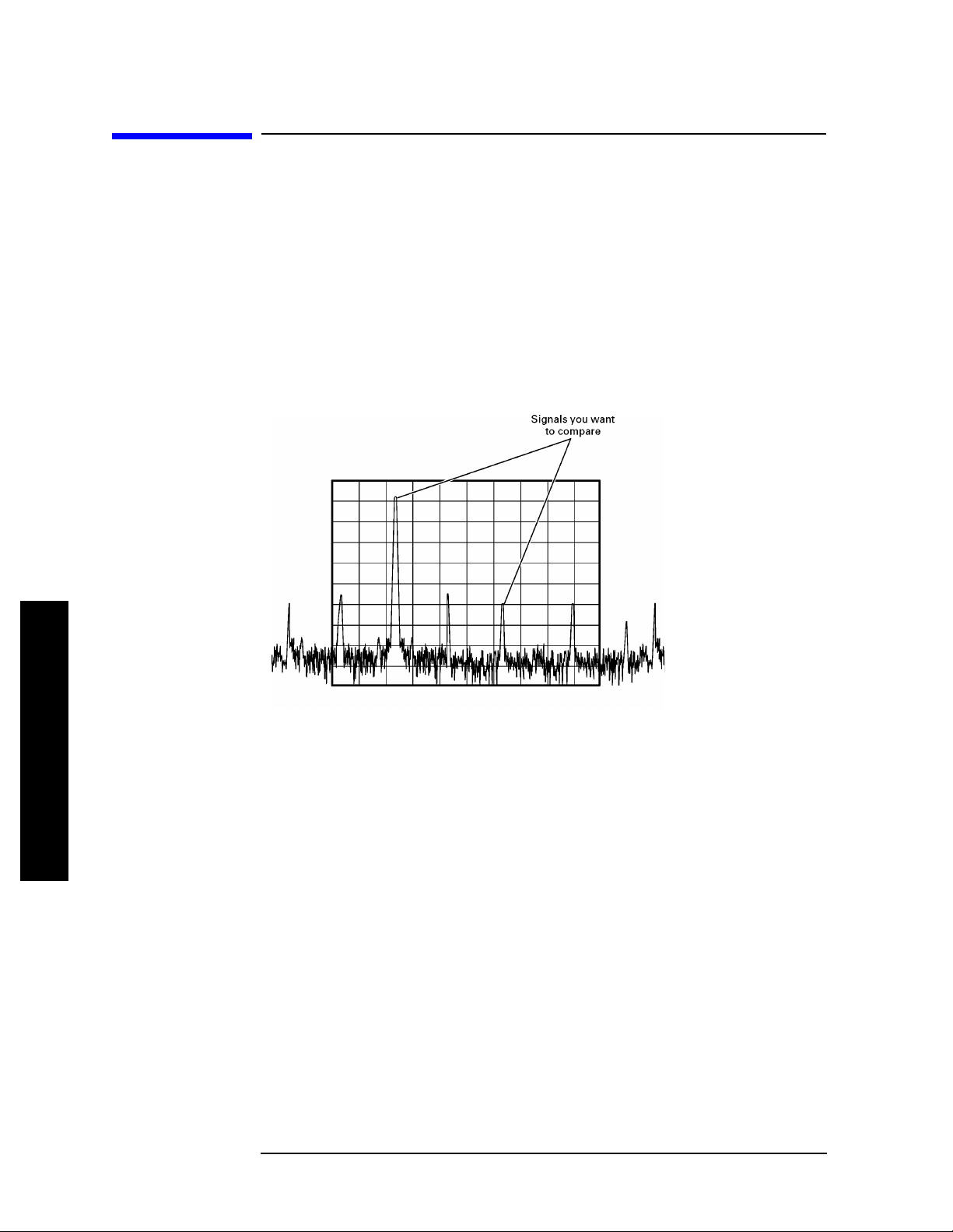
Using the analyzer, you can easily compare freque ncy and amplitude differences between signals, such as radio or television signal spectra. The analyzer delta marker function lets you compare two signals when both appear on the screen at one time .

In this procedure, the analyzer 10 MHz signal is used to measure frequency and amplitude differences between two signals on the same screen. Delta marker is used to demonstrate this comparison.

Figure 2-1 An Example of Comparing Signals on the Same Screen

Step 1. Preset the an alyzer:

Press

Step 2. (PSA)

Preset, Factory Preset (if present).

a. Enable the rear panel 10 MHz output.

Measuring Multiple Signals

Press

System, Reference, 10 MHz Out (On).

b. Connect the 10 MHz OUT (SWITCHED) from the rear panel to t he front panel RF input.

(ESA) Connect the rear panel 10 MHz REF OUT to the front panel RF input.

Step 3. Set the analyzer center frequency, span and reference level to view the

10 MHz signal and its harmonics up to 50 MHz: Press

Press Press

12 Chapter 2

FREQUENCY Channel, Center Freq, 30, MHz. SPAN X Scale, Span, 50, MHz. AMPLITUDE Y Scale, Ref Level, 10, dBm.

Measuring Multiple Signals

Comparing Signals on the Same Screen Using Marker Delta

Step 4. Place a marker at the highest peak on the display (10 MHz):

Press The

Peak Search.

Next Pk Right and Next Pk Left softkeys are available to move the

marker from peak to peak. The marker should be on the 10 MHz reference si g n a l :

Step 5. Anchor the first marker and activate a second marker:

Press

Marker, Delta.

The label on the first marker now reads 1R , indicating that it is the reference point.

Step 6. Move the second marker to another signal peak using the front-panel

knob or by using the Press

Press

Peak Search, Next Peak or Peak Search, Next Pk Right or Next Pk Left.

Peak Search key:

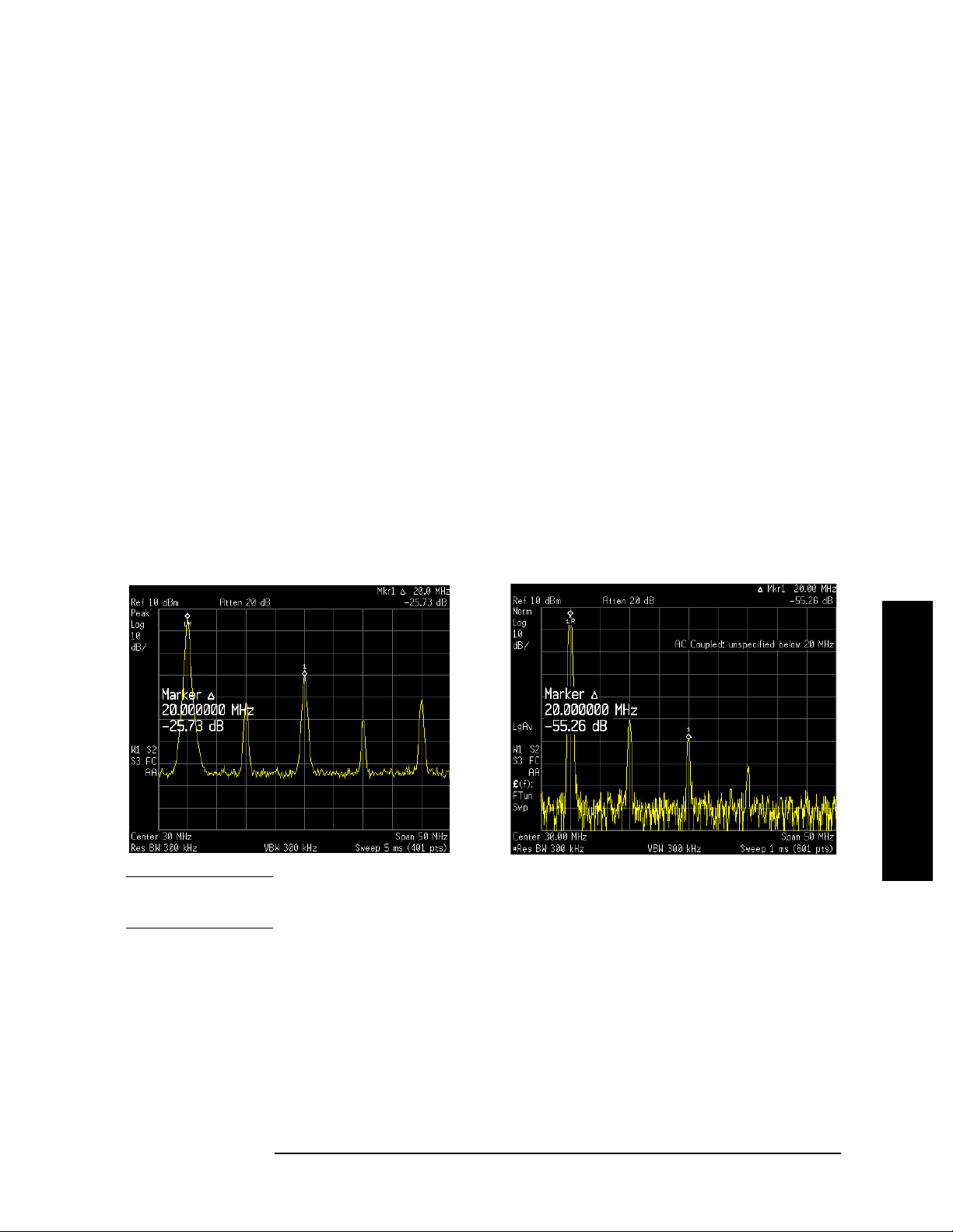
The amplitude and frequency difference between the markers is displayed in the active function block. For ESA see the lef t side of

Figure 2-2 and the right side for PSA.

Figure 2-2 Using the Delta Marker Function (ESA left, PSA right)

NOTE The resolution of the marker readings can be increased by turning on

the frequency count function.

Measuring Multiple Signals

Chapter 2 13

Measuring Multiple Signals

Comparing Signals on the Same Screen Using Marker Delta Pair

In this procedure, the analyzer 10 MHz signal is used to measure frequency and amplitude differences between two signals on the same screen using the delta pair marker function.

Step 1. Refer to the previous procedure “Comparing Signals on the Same

Screen Using Marker Delta” on page 12 and follow steps 1, 2 and 3.

Step 2. Turn on Delta Pair reference marker to compare the 10 MHz signal and

the 30 M Hz signal: Press Note that the

Step 3. Use the knob or Peak Search to move the second marker (labeled 1) to

Peak Search, Marker, Delta Pair (ref).

Delta Pair marker does not anchor the first marker.

the 30 MHz peak: Press

Step 4. Use the front panel knob to move the ref marker to the 20 MHz peak:

Peak Search, Next Peak or Next Pk Right.

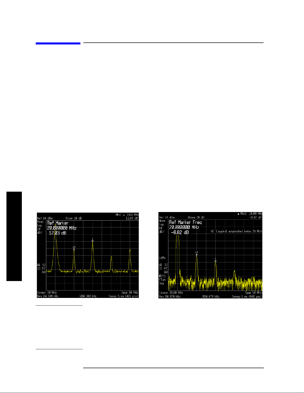
The active function displays the amplit ude and frequency difference between the 20 MHz and 30 MHz peaks as shown in Figure 2-3.

Figure 2-3 Using the Delta Pair Marker Function (ESA left, PSA right)

Measuring Multiple Signals

NOTE In Figure 2-3 notice that the active function reado ut has moved to the

top left of the analyzer display. The active function position has three positions: top, center and bott om. To modify the active function pos ition:

Press

Display, Active Fctn Position, Top (Center, or Bottom).

Center position is the factory default setting.

14 Chapter 2

Measuring Multiple Signals

Comparing Signals not on the Same Screen Using Marker Delta

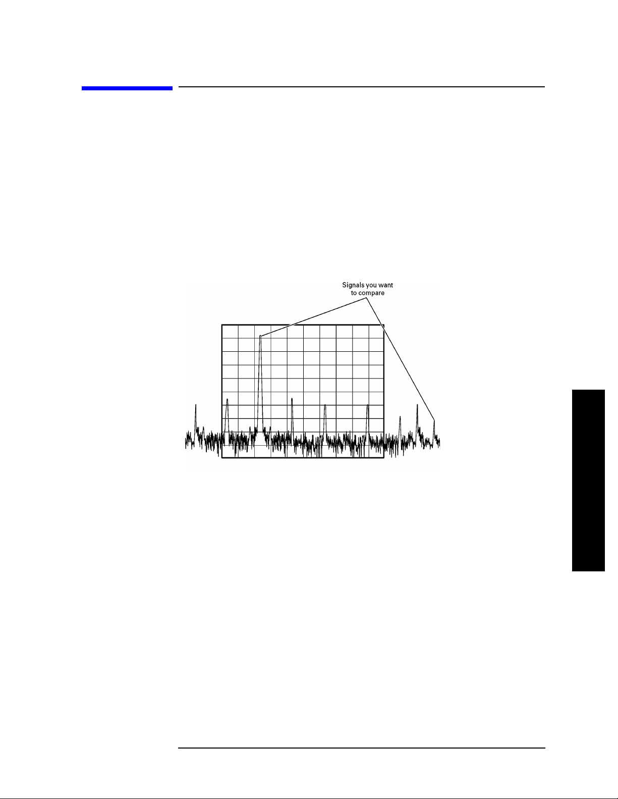
Measure the frequency and amplitude difference between two signals that do not appear on the screen at one time. (This technique is useful for harmonic distortion tes ts when narr ow span and narrow b andwidth are necessary to measure the low level harmonics.)

In this procedure, the analyzer 10 MHz signal is used to measure frequency and amplitude differences bet we en one signal on screen and one signal off screen. Delta marker is used to demonstrate this comparison.

Figure 2-4 Comparing One Signal on Screen with One Signal Off Screen

Step 1. Preset the an alyzer:

Press

Step 2. (PSA)

a. Enable the rear panel 10 MHz output: Press b. Connect the 10 MHz OUT (SWITCHED) from the rear panel to t he front

panel RF input: (ESA)

Connect the rear panel 10 MHz REF OUT to the front panel RF input.

Preset, Factory Preset (if present).

System, Reference, 10 MHz Out (On).

Measuring Multiple Signals

Chapter 2 15

Measuring Multiple Signals

Comparing Signals not on the Same Screen Using Marker Delta

Step 3. Set the center frequency, span and reference level to view only the

10 MHz signal: Press

Press Press

Step 4. Place a marker on the 10 MHz peak and then set the center frequency

FREQUENCY Channel, Center Freq, 10, MHz. SPAN X Scale, Span, 5, MHz. AMPLITUDE Y Scale, Ref Level, 10, dBm.

step size equal to the marker frequency (10 MHz): Press

Press

Step 5. Activate the marker delta function:

Press

Step 6. Increase the center frequency by 10 MHz:

Press

Peak Search. Marker →, Mkr → CF Step.

Marker, Delta.

FREQUENCY Channel, Center Freq, ↑.

The first marker moves to the left edge of the screen, at the amplitude of the first sign a l peak.

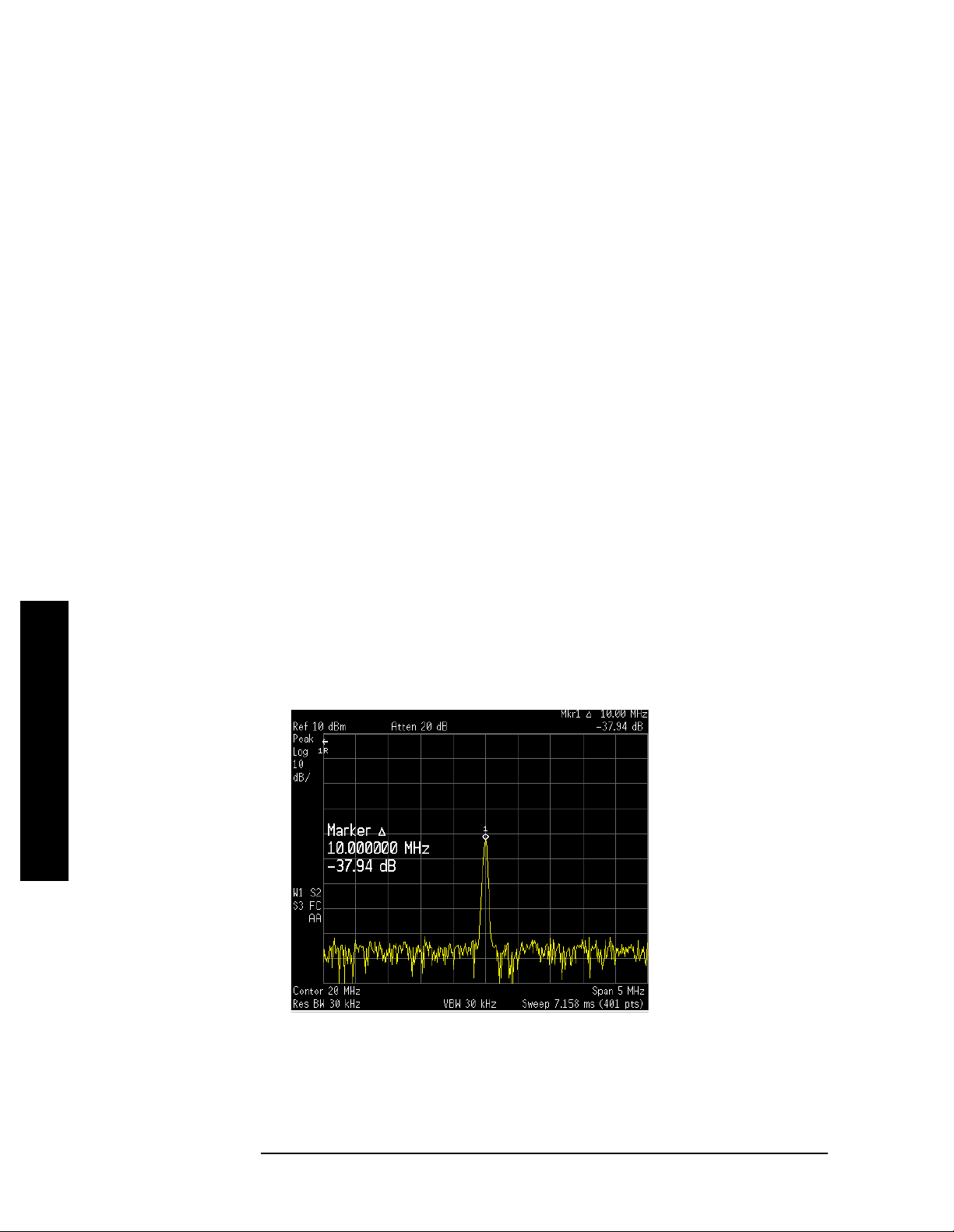
Figure 2-5 shows the reference annotation for the delta marker (1R) at

the left side o f th e display, indicating that th e 10 MHz refere n ce si g n a l is at a lower frequency than the frequency range currently displayed.

The delta marker appears on the peak of the 20 MHz component. The delta marker annotation displays the amplitude and frequency difference between the 10 and 20 MHz signal peaks.

Figure 2-5 Delta Marker with Reference Signal Off-Screen (ESA)

Measuring Multiple Signals

Step 7. Turn the markers off:

Press

Marker, Off.

16 Chapter 2

Resolving Signals of Equal Amplitude

In this procedure a decrease in resol ution bandwidth is used in combination with a decrease in video bandwidth to resolve two signals of equal amplitude with a freq uency s eparation of 100 kHz. Notice that the final RBW selection to resolve the signals is the same width as the signal separation while the VBW is slightly narrowe r than the RBW.

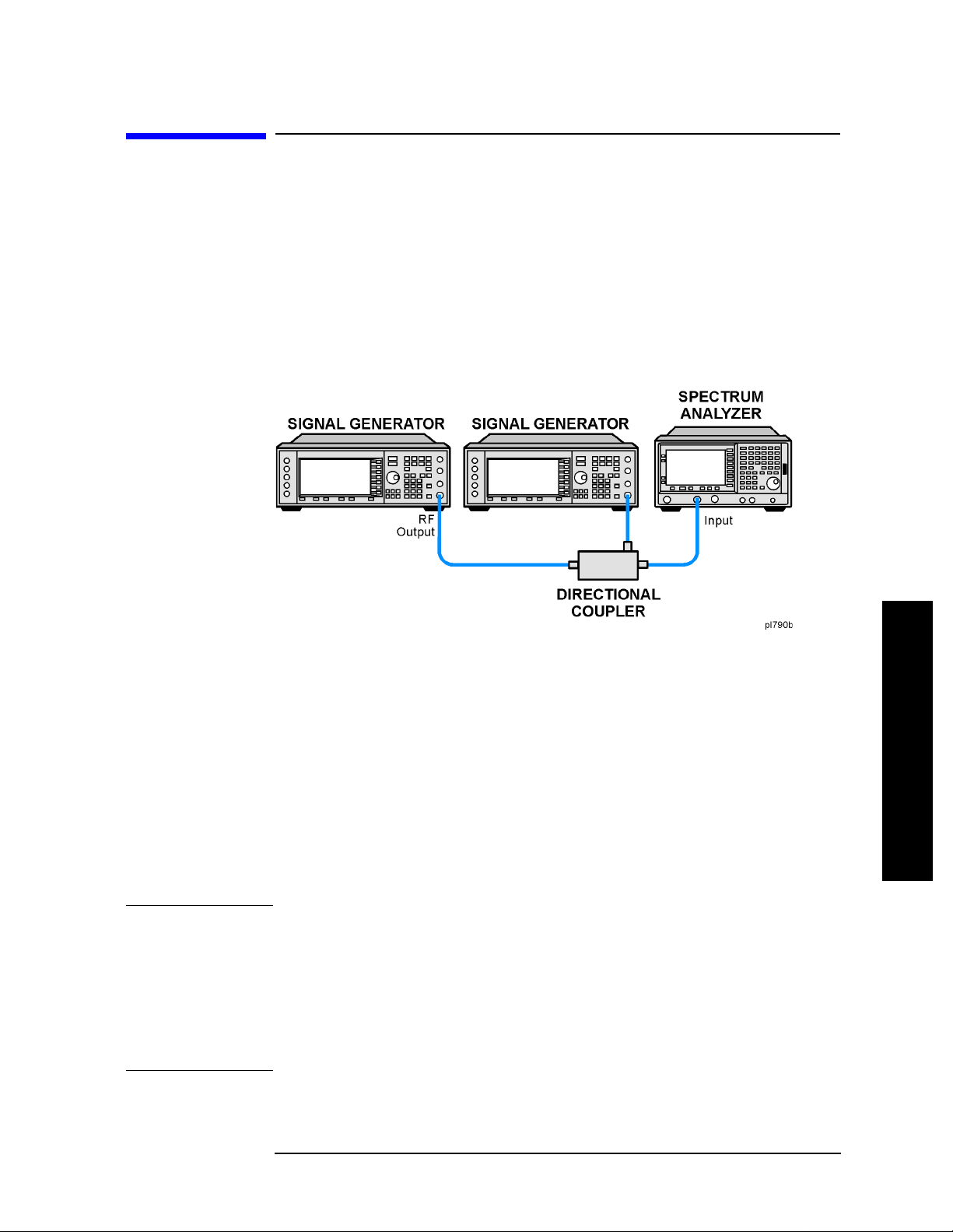
Step 1. Connect two sources to the analyzer input as shown in Figure 2-6.

Figure 2-6 Setup for Obtaining Two Signals

Measuring Multiple Signals

Resolving Signals of Equal Amplitude

Step 2. Set one source to 300 MHz. Set the frequency of the other source to

300.1 MHz. Set both source amplitudes to both signals should be approximately

−20 dBm. The amplitude of

−20 dBm at the output of the

bridge.

Step 3. Setup the analyzer to view the signals:

Press Press

Preset, Factory Preset (if present). FREQUENCY Channel, Center Freq, 300, MHz.

Press BW/Avg, Res BW, 300, kHz. Press

SPAN X Scale, Span, 2, MHz.

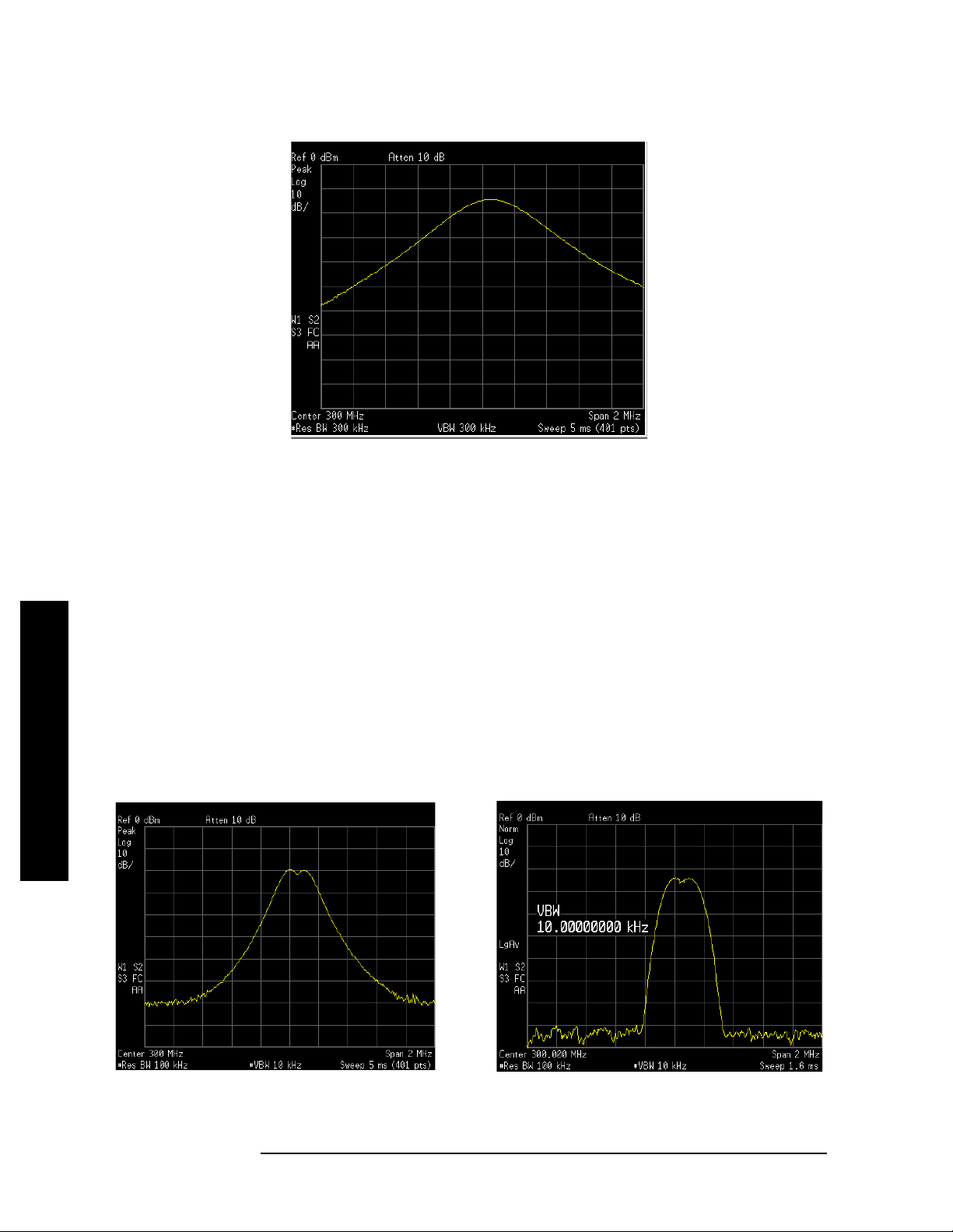
A single signal peak is visible. See Figure 2-7 for an ESA example.

NOTE If the signal peak is not present on the display, span out to 20 MHz,

turn signal tracking on, span back to 2 MHz and turn signal tracking off.:

Press Press Press

SPAN, Span, 20, MHz. Peak Search, FREQUENCY, Signal Track (On). SPAN, 2, MHz.

Press FREQUENCY, Signal Track (Off)

Measuring Multiple Signals

Chapter 2 17

Measuring Multiple Signals

Resolving Signals of Equal Amplitude

Figure 2-7 Unresolved Signals of Equal Amplitude (ESA)

Step 4. Change the resolution bandwidth (RBW) to 100 kHz so that the RBW

setting is less than or equal to the frequency separation of the two signals:

Press

BW/Avg, Res BW, 100, kHz.

Notice that the peak of the signal has become flattened indicating that two signals may be present .

Step 5. Decrease the vi d e o b a n dw i dth to 10 kHz:

Press

Video BW, 10, kHz.

Two signals are now visible as shown with the ESA on the left side in

Figure 2-8 and the PSA on the right side. Use the front-panel knob or

step keys to further reduce the resolution bandwidth and better resolve the signals.

Figure 2-8 Resolving Signals of Equal Amplitude (ESA left, PSA right)

Measuring Multiple Signals

18 Chapter 2

Measuring Multiple Signals

Resolving Signals of Equal Amplitude

As the resolution bandwidth is decreased, resolution of the individual signals is improved and the sweep time is increased. For fastest measurement times, use the widest possible resolution bandwidth. Under factor y pr eset conditi o n s, the re so l u ti on bandwidt h is “coupled” (or linked) to the span.

Since the resolution bandwidth has been changed from the coupled value, a # mark appears next to Res BW in the lower-left corner of the screen, indicating that the resolution bandwidth is uncoupled. (For more infor m a ti on on coupli n g, ref e r to the

Auto Couple key descr i ption

in the Agilent Technologies ESA Spectrum Analyzers User’s/Programmer’s Reference Guide and the PSA Spectrum Analyzers User’s/Programmer’s Reference Guide.)

NOTE To res olve two signals of equal amplitude with a frequency separation

of 200 kHz, the resolution bandwidth must be less than the signal separation so a resolution bandwidth of 100 kHz must be used. (For analyzers that use a 1-3-10 RBW step sequence, a 100 kHz RBW is the best choice for signal separation, but for high performance analyzers, like the PSA, a 180 kHz RBW can be selected by fine tuning the RBW filters at 10% increments.) Filter widths above 200 kHz exceed the 200 kHz signal separation and would not resolve the signals.

Measuring Multiple Signals

Chapter 2 19

Measuring Multiple Signals

Resolving Small Signals Hidden by Large Signals

This procedure uses narrow resoluti on bandwidths to res olve two input signals with a frequency separation of 155 kHz and an amplitude difference of 60 dB .

Step 1. Connect two sources to the analyzer input as shown in Figure 2-6. Step 2. Set one source to 300 MHz at −10 dBm. Set the second source to

300.05 MHz, so that the signal is 50 kHz higher than the first signal. Set the amplitude of the signal to signal).

Step 3. Set the analyzer as follows:

−70 dBm (60 dB below the first

Press Press Press Press

NOTE If the signal peak is not present on the display, span out to 20 MHz,

Preset, Factory Preset (if present). FREQUENCY Channel, Center Freq, 300, MHz. BW/Avg, 30, kHz. SPAN X Scale, Span, 500, kHz.

turn signal tracking on, span back to 2 MHz and turn signal tracking off:

Press Press Press

SPAN, Span, 20, MHz. Peak Search, FREQUENCY, Signal Track (On). SPAN, 2, MHz.

Press FREQUENCY, Signal Track (Off).

Step 4. Set the 300 MHz signal to the reference level:

Press

Measuring Multiple Signals

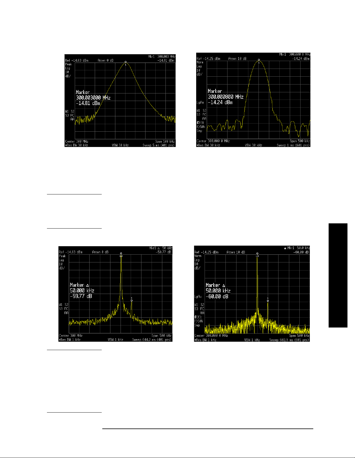
NOTE The ESA 30 kHz filter shape factor of 15:1 (PSA is 4.1:1) has a

bandwidth of 450 kHz at the 60 dB point (PSA has a BW of 123 kHz).

Peak Search, Mkr →, Mkr → Ref Lvl.

The half-bandwidth (225 kHz for ESA and 61.5 kHz for PSA) is NOT narrower than the frequency separation of 50 kHz, so the input signals can not be resolved.

20 Chapter 2

Measuring Multiple Signals

Resolving Small Signals Hidden by Large Signals

Figure 2-9 Signal Resolution with a 30 kHz RBW (ESA left, PSA right)

Step 5. Reduce the resolution bandwidth filter to view the smaller hidden

signal. Place a delta marker on the smaller signal: Press

Press

NOTE The ESA 1 kHz filter shape factor of 15:1 (PSA is 4.1:1) has a

BW/Avg, 1, kHz. Peak Search, Marker, 50, kHz.

bandwidth of 15 kHz at the 60 dB point (PSA has a BW of 4.1 kHz). The half-bandwidth (7.5 kHz for ESA and 2.05 kHz for PSA) is narrower than 50 kHz, so the input signals can be resolved.

Figure 2-10 Signal Resolution with a 1 kHz RBW (ESA left, PSA right)

Measuring Multiple Signals

NOTE To determine the resolution capability for intermediate amplitude

differences, assume the filter skirts between the 3 dB and 60 dB points are parabolic, like an ideal Gaussian filter. The resolution capability is approximately:

∆f



12.04 dB

-------------

•



RBW

where ∆f is the separation between the signals.

Chapter 2 21

Measuring Multiple Signals

Decreasing the Frequency Span Around the Signal

Using the analyzer signal track func tion, you can quickly decrease the span while keeping the signal at center frequency. This is a fast way to take a closer look at the area around the signal to identify signals that would otherwise not be resolved.

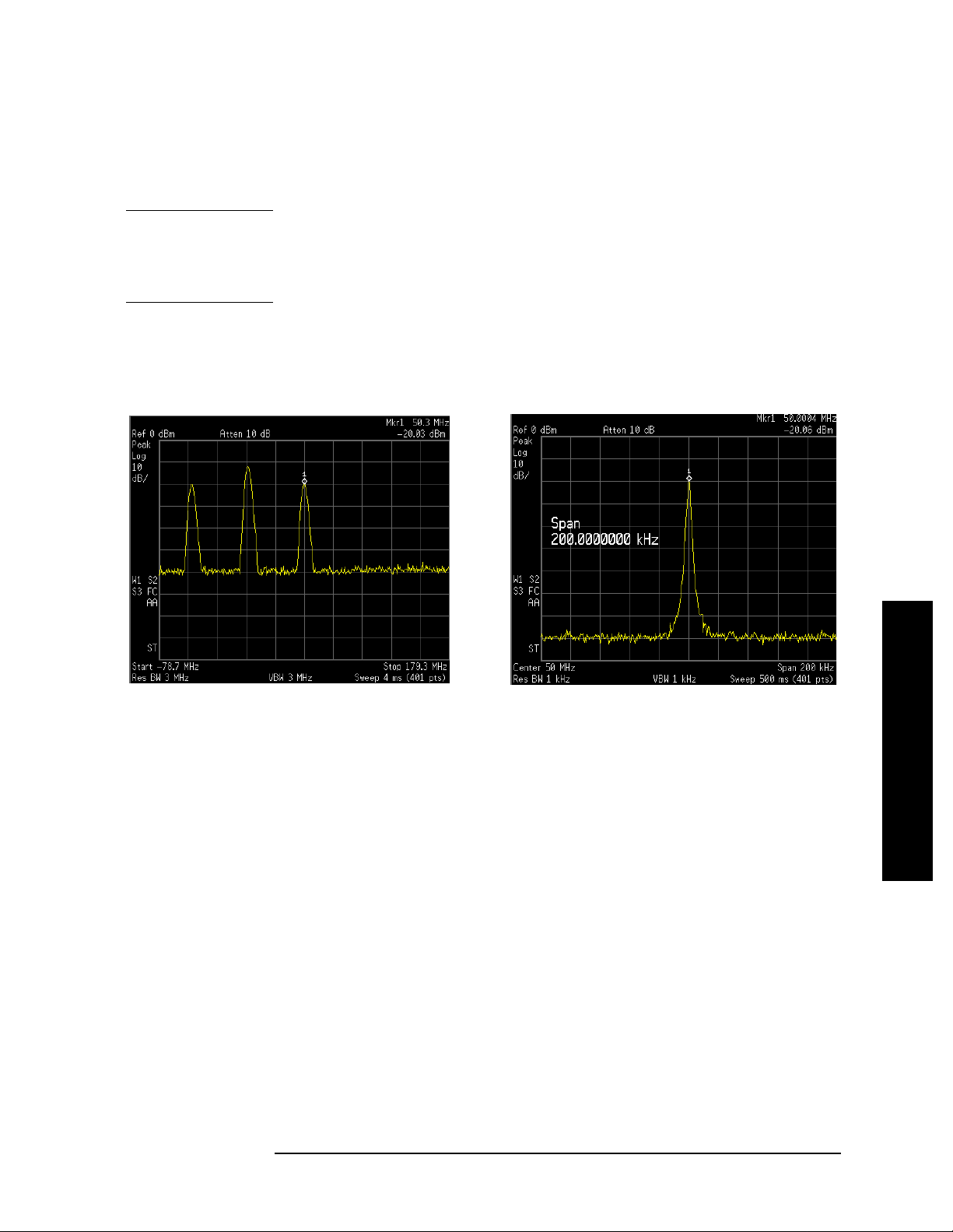
This procedure uses signal trac king and span zoom to view the analyzer 50 MHz reference signal in a 200 kHz span.

Step 1. Perform a factory preset:

Press

Step 2. Enable the internal 50 MHz amplitude reference signal of the analyzer

Preset, Factory Preset (if present).

as follows: (PSA)

Press

Input/Output, Input Port, Amptd Ref.

(ESA E4401B and E4411B) Press

Input/Output, Amptd Ref (On).

(ESA E4402B, E4403B, E4404B, E4405B, E4407B and E4408B) Connect a cable from the front panel AMPTD REF OUT to the analyz er RF input: Press

Step 3. Set the start frequency to 20 MHz and the stop frequency to 1 GHz:

Press Press

Step 4. Place a marker at the peak:

Press

Measuring Multiple Signals

Step 5. Turn on the signal tracking function to move the signal to the center of

Input/Output, Amptd Ref Out (On).

FREQUENCY Channel, Start Freq, 20, MHz. FREQUENCY Channel, Stop Freq, 1, GHz.

Peak Search.

the screen (if it is not already positioned there): Press

FREQUENCY Channel, Signal Track (On).

See the left-side of figure Figure 2-11. (Note that the marker must be on the signal before turning signal track on.)

NOTE Because the signal track f unction automaticall y maintains the sig nal at

the center of the screen, you can reduce the span quic k l y for a closer look. If the signal drifts off of the screen as you decrea se the span, use a wider frequency span. (You can also use as a quick way to perform the

SPAN key sequence.)

22 Chapter 2

Peak Search, FREQUENCY, Signal Track,

Span Zoom, in the SPAN menu,

Measuring Multiple Signals

Decreasing the Frequency Span Around the Signal

Step 6. Reduce span and resolution bandwidth to zoom in on the marked

signal: Press

NOTE If the span change is large enough, the span decreases in steps as

SPAN X Scale, Span, 200, kHz.

automatic zoom is completed . See Figure 2-11 on the right side. You can also use the front-panel knob or step k eys to decrease the span and resolution bandwidth values.

Step 7. Turn off signal tracking:

Press

FREQUENCY Channel, Signal Track (Off).

Figure 2-11 Signal Tracking

LEFT: Signal tracking on before span decrease RIGHT: After zooming in on the signal

Measuring Multiple Signals

Chapter 2 23

Measuring Multiple Signals

Decreasing the Frequency Span Around the Signal

Measuring Multiple Signals

24 Chapter 2

3 Measuring a Low−Level Signal

Measuring a Low

−

Level Signal

Measuring a Low−Level Signal

Reducing Input Attenuation

The ability to measure a low-level signal is limited by internally generated noise in the spectrum analyzer. The measurement setup can be changed in several ways to improve the analyzer sensitivity.

The input attenuator affects the level of a signal pas sing through the instrument. If a signal is very close to the noise floor, reducing input attenuation can bring the signal out of the noise.

CAUTION Ensure that the total power of all input signals at the analyzer RF

input does not exceed +30 dBm (1 watt).

Step 1. Preset the an a l y z er:

Press Preset, Factory Preset (if present).

Step 2. Set the freque n cy o f th e si g n a l so u r ce to 30 0 MHz. Set the source

amplitude to RF INPUT.

−80 dBm. Connect the source RF OUTPUT to the analyzer

Step 3. Set the center frequency, span and reference level:

Press Press Press

FREQUENCY Channel, Center Freq, 300, MHz. SPAN X Scale, Span, 5, MHz. AMPLITUDE Y Scale, Ref Level, 40, −dBm.

Step 4. Move the desired peak (in this example, 300 MHz) to the center of the

display: Press

Peak Search, Marker ➞, Mkr ➞ CF.

Step 5. Reduce the span to 1 MHz (as shown in Figure 3 -1) and if necessary

re-center the peak: Press

Span, 1, MHz.

Figure 3-1 Measuring a Low-Level Signal (ESA Display)

Level Signal

−

Measuring a Low

26 Chapter 3

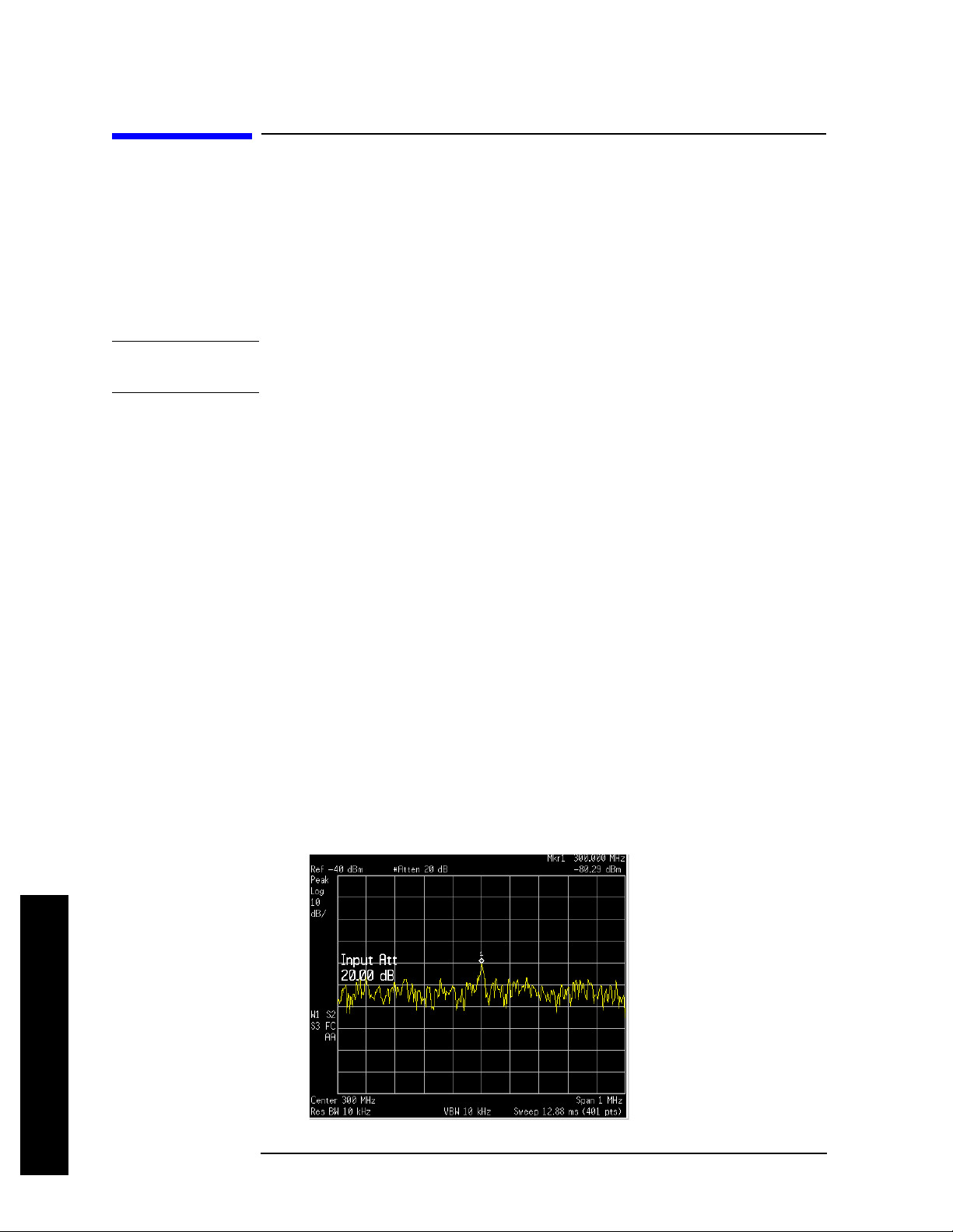
Step 6. Set the attenuation to 20 dB:

Measuring a Low−Level Signal

Reducing Input Attenuation

Press

AMPLITUDE Y Scale, Attenuation, 20, dB.

Note that increasing the attenuation moves the noise floor closer to the signal level.

A “#” mark appears next to the Atten annotation at the top of the display, indicating that the attenuation is no longer coupled to other analyzer settings.

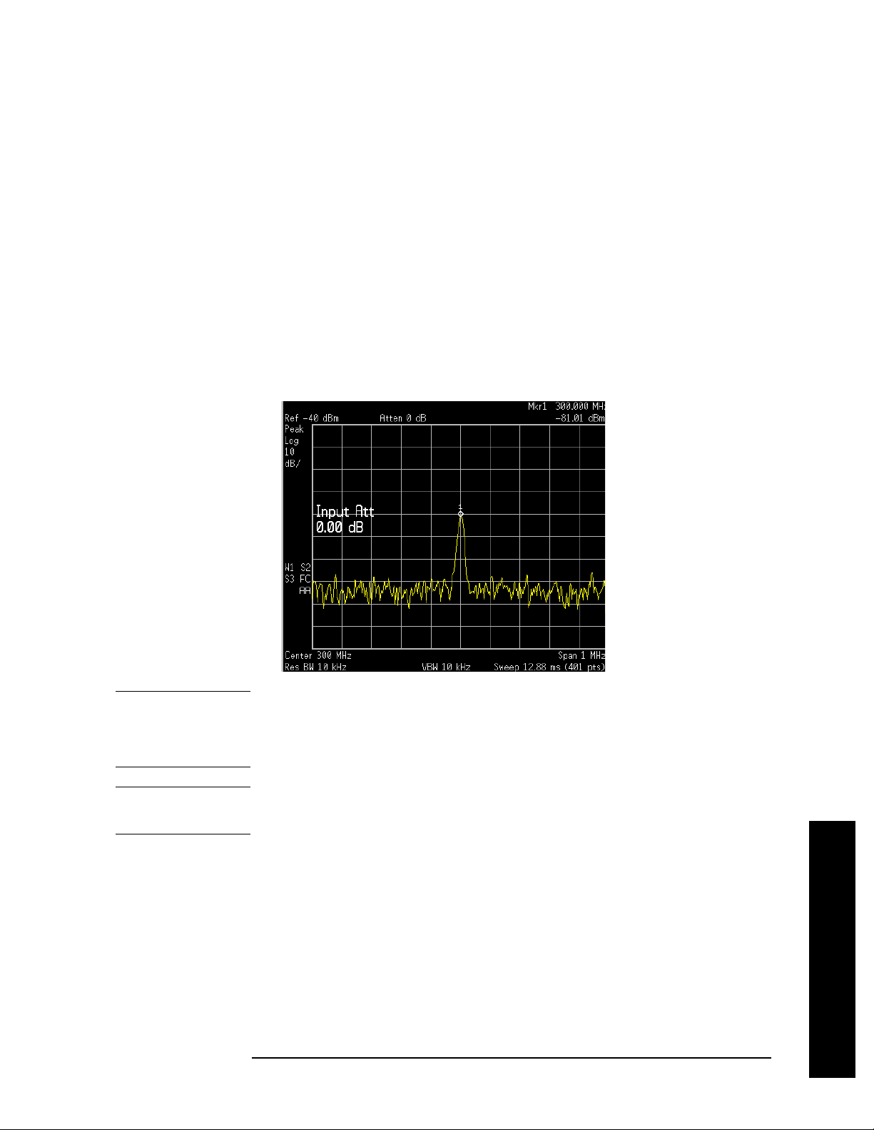
Step 7. To see the signal more clearly, set the attenuation to 0 dB:

Press

AMPLITUDE, Attenuation, 0, dB.

See Figure 3-2 shows 0 dB input attenuation.

Figure 3-2 Measuring a Low-Level Signal Using 0 dB Attenuation (ESA)

CAUTION When you finish this example, increase the attenuation to protect the

analyzer’s RF inpu t: Press AMPLITUDE Y Scale, Attenuation (Auto) or press Auto Couple.

NOTE All figures in this chapter are screen captures from an ESA. Display

and numerical results may be different for a PSA.

Chapter 3 27

Measuring a Low

−

Level Signal

Measuring a Low−Level Signal

Decreasing the Resolution Bandwidth

Resolution bandwidth settings affect the level of internal noise without affecting the level of continuous wave (CW) signals. Decreasing the RBW by a decade reduces the noise floor by 10 dB.

Step 1. Refer to the first procedure “Reducing In put Attenuation” on page 26 of

this chapter and follow steps 1, 2 and 3.

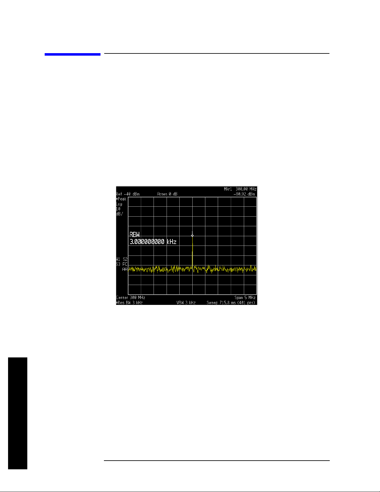
Step 2. Decrease the resolution bandwidth:

Press

BW/Avg, ↓.

The low-level signal appears more clearly because the noise level is reduced (see Figure 3-3).

Figure 3-3 Decreasing Resolution Bandwidth

A “#” mark appears next to the Res BW annotation in the lower left corner of the screen, indicating that the resolution bandwidth is uncoupled.

RBW Selections You can use the step keys to change the RBW in a 1

−3−10 sequence.

For ESA, RBWs below 1 kHz are digital and have a selectivity ratio of 5:1 while RBWs at 1 kHz and higher have a 15:1 selectivity ratio. The ESA’s maximum RBW is 5 MHz a nd the minimum is 1 Hz (optional).

All PSA RBWs are digital and have a selectivity ratio of 4.1:1. For PSA, choosing the next lower RBW for better sensitivity increases the sweep

Level Signal

−

time by about 10:1 for swept measurements, and about 3:1 for FFT measurements (within the limits of RBW). Using the knob or keypad, you can select RBWs from 1 Hz to 3 MHz in approximately 10% increments, plus 4, 5, 6 and 8 MHz. This enables you to make the trade off between sweep tim e a n d se n s i t ivity with finer resolut i on.

Measuring a Low

28 Chapter 3

Measuring a Low−Level Signal

Using the Average Detector and Increased Sweep Time

When the analyzer’s noise masks low-level signals, changing to the average detector and increasing the sweep time smooths the noise and improves the signal’s visibility. Slower sweeps are required to average more noise variations.

Step 1. Refer to the first procedure “Reducing In put Attenuation” on page 26 of

this chapter and follow steps 1, 2 and 3.

Step 2. Select the average detector:

Press

Det/Demod, Detector, Average.

A “#” mark appears next to the Avg annotation, indicating that the detector has been chosen manually (see Figure 3-4).

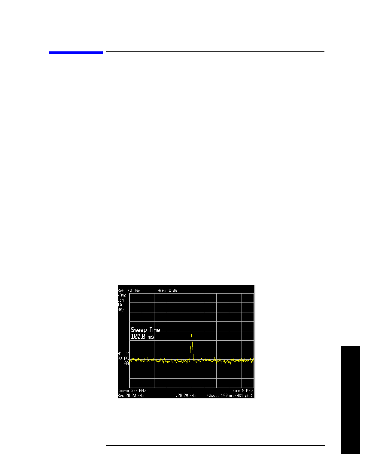
Step 3. Increase the sweep time to 100 ms:

Press

Sweep, Sweep Time, ↑.

Note how the noise smooths out, as there is more time to average the values for each of the displ ayed data points .

Step 4. With the sweep time at 100 ms, change the average type to

log averaging: (ESA) Press

(PSA) Press

BW/Avg, Avg Type, Video Avg. BW/Avg, Avg/VBW Type, Log-Pwr.

Figure 3-4 Varying the Sweep Time with the Average Detector

Chapter 3 29

Measuring a Low

−

Level Signal

Measuring a Low−Level Signal

Trace Averaging

Averaging is a digital proces s in which each trace point is aver aged with the previous average for the same trace point. Selecting averaging, when the analyzer is autocoupled, changes the detection mode (from peak in ESA and normal in PSA) to sample, smoothing the displa ye d noise level. ESA sample mode displays the instantaneous value of the signal at the end of the time or frequency interval represented by each display point (for PSA it is t he ce nter of the t ime or fr equency interval), rather than the value of the peak during the interval. Sample mode may not measure a signal’s amplitude as accurately as normal mode, because it may not find the true peak.

NOTE This is a trace processing function and is not the same as using the

average detector (as described on page 29).

Step 1. Refer to the first procedure “Reducing In put Attenuation” on page 26 of

this chapter and follow steps 1, 2 and 3.

Step 2. Turn video averaging on:

Press

BW/Avg, Average (On).

As the averaging routine smooths the trace, low level signals become more visible. Average 100 appears in the active function block.

Step 3. With average as the active function, set the number of averages to 25:

Press

25, Enter.

Annotation on the left side of the graticule shows the type of averaging (the annotation for ESA is VAvg and is LgAv for PSA), and the number of traces averaged.

Changing most active functions res tarts the averag ing , as do es toggling

Average key. Once the set number of sweeps com pletes , the analyzer

the continues to provide a running average based on this se t nu mbe r.

NOTE If you want the measurement to stop after the set number of sweeps,

use single sweep: Press

Sweep, Sweep (to select Single), or press Single

and then toggle the Average key.

Level Signal

−

Measuring a Low

30 Chapter 3

and Accuracy

Improving Frequency Resolution

4 Improving Frequency Resolution

and Accuracy

Improving Frequency Resolution and Accuracy

Using a Frequency Counter to Improve Frequency Resolution and Accuracy

Using a Frequency Counter to Improve

Improving Frequency Resolution

and Accuracy

Frequency Resolution and Accuracy

This procedure uses the spectrum analyzer internal frequency counter to increase the resolution and accuracy of the frequency readout.

Step 1. Preset the an alyzer:

Press

Step 2. Enable the internal 50 MHz amplitude reference signal as follows:

Preset, Factory Preset (if present).

(PSA) Press

Input/Output, Input Port, Amptd Ref.

(ESA E4401B and E4411B) Press

Input/Output, Amptd Ref (On).

(ESA E4402B, E4403B, E4404B, E4405B, E4407B and E4408B) Connect a cable from the front panel AMPTD REF OUT to the analyz er RF input: Press

Step 3. Set the center frequency to 50 MHz and the span to 80 MHz:

Press Press

Input/Output, Amptd Ref Out (On).

FREQUENCY Channel, Center Freq, 50, MHz. SPAN X Scale, Span, 80, MHz.

Step 4. Turn the frequency counter on:

(ESA) Press

Freq Count.

(PSA) Press Marker Fctn, Marker Count, Marker Count (On).

NOTE The frequency and amplitude of the marker and the word Marker

appears in the active function area (this is not the counte d res ult). The counted resu l t ap pears in the uppe r-righ t co rner of the dis pl ay to the right-side of Cntr1.

Step 5. Move the marker, with the front -panel k nob , half -way down the skirt of

the signal respon se. Notice that the readout in the active frequency function changes while

the counted frequency result (upper-right corner of display) does not. See Figure 4-1. To get an accurate count, you do not need to place the marker at the exact peak of the signal response.

NOTE Marker count properly functions on ly on CW signals or discrete spect ral

components. The marker must be

> 25 dB above the displayed noise

level.

32 Chapter 4

Improving Frequency Resolution and Accuracy

Using a Frequency Counter to Improve Frequency Resolution and Accuracy

Figure 4-1 Using Marker Counter (ESA Display)

Step 6. Change counter resolution:

Improving Frequency Resolution

and Accuracy

ESA frequency-counter resolution can be set from 1 Hz to 100 kHz by pressing

Freq Count, Resolution.

PSA frequency-counter resolution is fixed at 0.001 Hz for 2 ms and longer gate times. Longer gate times allow for greater averaging of signals whose frequency is "noisy", at the expense of throughput.

NOTE For PSA, if the Gate Time (under the Marker Count menu) is an integer

multiple of the length of a power-line cycle (20 ms for 50 Hz power,

16.67 ms for 60 Hz power), the counter rejects incid ental modulation at the power line rate. The shortest Hz modulation is 100 ms (100 ms is the default

Gate Time that rejects both 50 and 60

Gate Time setting when

set to Auto).

Step 7. The marker counter remains on until turned off. Turn off the marker

counter: (ESA) Press

(PSA) Press

Marker, Off.

NOTE When using the built-in frequency counter func tion with the ESA, if the

Freq Count, Marker Count (Off). Or Press Marker, Off. Marker Fctn, Marker Count, Marker Count (O ff) . O r Pr e s s

ratio of the resolution bandwidth to the span is too small (less than or equal to 0.002), the Marker Count: Widen Res BW message appears on the display. It indicates that the resolution bandwidth is too narrow.

Chapter 4 33

Improving Frequency Resolution

Improving Frequency Resolution and Accuracy

Using a Frequency Counter to Improve Frequency Resolution and Accuracy

and Accuracy

34 Chapter 4

Tracking Drifting Signals

5 Tracking Drifting Signals

Tracking Drifting Signals

Measuring a Source’s Frequency Drift

The analyzer can measure the short- and long-term stability of a source. The maximum amplitude level and the frequency dr ift of an input signal trace can be displayed and held by using the maximum-hold function. You can also use the maximum hold function if you want to determine how much of the frequency spectrum a signal occupies.

This procedure using signal tracking to keep the drifting signal in the center of the display. The drifting is captured by the analyzer using maximum h old.

Step 1. Connect the signal generator to the analyzer input. Step 2. Set the signal generator frequency to 300 MHz with an amplitude of

−20 dBm.

Step 3. Set the analyzer center frequency, span and reference level.

Tracking Drifting Signals

Press Press Press Press

Step 4. Place a marker on the peak of the signal and turn signal tracking on:

Press Press

Preset, Factory Preset (if present). FREQUENCY Channel, Center Freq, 300, MHz. SPAN X Scale, Span, 10, MHz. AMPLITUDE Y Scale, Ref Level, 10, −dBm.

Peak Search. FREQUENCY Channel, Signal Track (On).

Reduce the span to 500 kHz: Press

SPAN, Span Zoom, 500, kHz.

Notice that th e si g n a l is held in the ce n t er of the display.

Step 5. Turn off the signal track function:

Press

Step 6. Measure the excursion of the signal with maximum hold:

(ESA) Press (PSA) Press

FREQUENCY Channel, Signal Track (Off).

View/Trace, Max Hold.

Trace/View, Max Hold.

As the signal varies, maximum hold maintains the maximum responses of the input signal.

NOTE Annotation on the left side of the screen indicates the trace mode. For

example, M1 S2 S3 indicates trace 1 is in maximum-hold mode, trace 2 and trace 3 are in store-blank mode.

36 Chapter 5

Tracking Drifting Signals

Measuring a Source’s Frequency Drift

Step 7. Activate trace 2 (trace 2 should be underlined) and change the mode to

continuous sweeping: (ESA) Press

(PSA) Press Press

Clear Write.

View/Trace, Trace (2). Trace/View, Trace (2).

Trace 1 remains in maximum hold mode to show any drif t in the signal.

Step 8. Slowly change the frequency of the signal generator ± 50 kHz in 1 kHz

increments. Your analyzer display should look similar to Figure 5-1.

Figure 5-1 Viewing a Drifting Signal With Max Hold and Clear Write

Tracking Drifting Signals

Chapter 5 37

Tracking Drifting Signals

Tracking a Signal

The signal track function is useful for tracking drifting signals that drift relatively slowly by keeping the signal centered on the display as the signal drifts. This procedure tracks a drifting signal.

Note that the primary function of the si gn al track function is to track unstable signals, not to track a signal as the center frequency of the analyzer is changed. If you choose to use the signal track function when changing center frequency, check to ensure that the signal found by the tracking function is the corre ct signal.

Step 1. Set the source frequency to 300 MHz with an amplitude of −20 dBm. Step 2. Set the analyzer center frequency at a 1 MHz offset:

Tracking Drifting Signals

Press Press Press

Step 3. Turn the signal tracking function on:

Press

Preset, Factory Preset (if present). FREQUENCY Channel, Center Freq, 301, MHz. SPAN X Scale, Span, 10, MHz.

FREQUENCY Channel, Signal Track (On).

Notice that signal tracking places a marker on the highest amplitude peak and then brings the selected peak to the center of the display. After each sweep the center frequency of the analyzer is adjusted to keep the selected peak in the center.

Step 4. Turn the delta marker on to read signal drift:

Press

Step 5. Tune the frequency of the signal generator in 100 kHz increments.

Marker, Delta.

Notice that the center frequency of the analyzer also c h anges i n 100 kHz increments, centering the signal with each increment.

Figure 5-2 Tracking a Drifting Signal (ESA left, PSA right)

38 Chapter 5

6 Making Distortion

Measurements

Making Distortion Measurements

Identifying Analyzer Generated Distortion

Identifying Analyzer Generated Di stortion

High level input signals may cause analyzer distortion products that could mask the real distortion measured on the input signal. Using trace 2 and the RF attenuator, you can determine which signals, if any, are internally generated distortion products.

Using a signal from a signal generator, determine whether the harmonic distortion products are generated by the analyzer.

Step 1. Connect the signal generator to the analyzer input. Step 2. Set the source frequency to 200 MHz with an amplitude of 0 dBm. Step 3. Set the analyzer center frequency and span:

Press Press Press

Preset, Factory Preset (if present). FREQUENCY Channel, Center Freq, 400, MHz. SPAN X Scale, Span, 500, MHz.

The signal produces harmonic distortion products (spaced 200 MHz from the original 200 MHz signal) in the analyzer input mixer as shown in Figure 6-1.

Figure 6-1 Harmonic Distortion (ESA left, PSA right)

Making Distortion Measurements

Step 4. Change the center frequency to the value of the first harmonic:

Press

Step 5. Change the span to 50 MHz and re-center the signal:

Press Press

Step 6. Set the attenuation to 0 dB:

Press

40 Chapter 6

Peak Search, Next Peak, Marker→, Mkr→CF.

SPAN X Scale, Span, 50, MHz. Peak Search, Marker→, Mkr→CF.

AMPLITUDE Y Scale, Attenuation, 0, dB.

Making Distortion Measurements

Identifying Analyzer Generated Distortion

Step 7. To determine whether the harmonic distortion products are generated

by the analyzer, firs t save the trace data in trace 2 as follows: (ESA) Press

(PSA) Press

Step 8. Allow trace 2 to update (minimum two sweeps), then store the data

View/Trace, Trace (2), Clear Write. Trace/View, Trace (2), Clear Write.

from trace 2 and place a delta marker on the harmonic of trace 2: Press

Press

View. Peak Search, Marker, Delta.

The analyzer display sho ws the stored data in trace 2 an d the measured data in trace 1. The

∆Mkr1 amplitude reading is the difference in

amplitude between the reference and active markers.

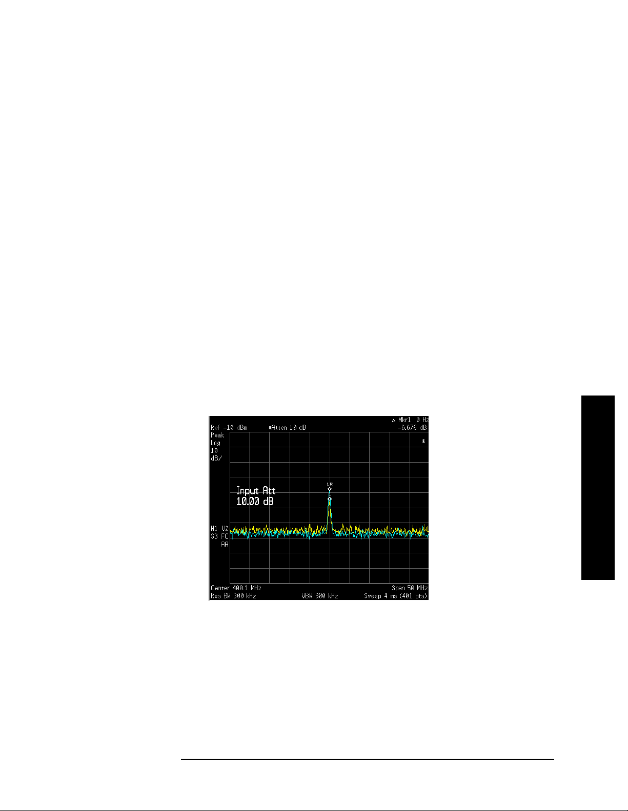
Step 9. Increase the RF attenuation to 10 dB:

Press Notice the

AMPLITUDE Y Scale, Attenuation, 10, dB.

∆Mkr1 amplitude reading. This is the difference in the

distortion product amplitud e readings between 0 dB and 10 dB input attenuation settings. If the approximately

≥1 dB for an input attenuator change, the distortion is

being generated, at least in part, by the analyzer. In this case more input attenuation is necessary. See Figure 6-2.

Figure 6-2 RF Attenuation of 10 dB

∆Mkr1 amplitude absolute value is

Making Distortion Measurements

∆Mkr1 amplitude reading comes from two sources:

The

1) Increased input attenuati on causes poorer signal-to-noise ratio. This can cause the

∆Mkr1 to be positive.

2) The reduced contribution of the analyzer circuits to the harmonic measurem e nt can cause t he

Large

∆Mkr1 measurements indicate significant measurement errors.

Set the input attenuator to minimize the absolute value of

Chapter 6 41

∆Mkr1 to be negative.

∆Mkr1.

Making Distortion Measurements

Third-Order Intermodulation Distortion

Two-tone, third-order intermodulation distortion is a common test in communication systems. When two signals are present in a non-linear system, they can interact and create third-order intermodulation distortion products that are located close to the original signals. These distortion products are generated by system components such as amplifiers and mixers.

For the quick setup TOI measurement example, refer to “Measuring

TOI Distortion with a One-Button Measurement” on page 44.

This procedure tests a device for third -order intermodulation using markers. Two sources are used, one set to 300 MHz and the other to 301 MHz.

Step 1. Connect the equipment as shown in Figure 6-3. This combination of

signal generators, low pass filters, and directional coupler (used as a combiner) results in a two-tone source with very low intermodulation distortion. Although the distortion from this setup may be better than the specified performance of the analyzer, it is useful for determining the TOI performance of the source/analyzer combination. After the performance of the source/analyzer combination has been verified, the device-under-test (DUT) (for example, an amplifier) would be inserted between the directional coupler output and the analyzer input.

Figure 6-3 Third-Order Intermodulation Equipment Setup

Making Distortion Measurements

NOTE The coupler should have a high degree of isolation between the two

input ports so the sources do not in termodulate.

Step 2. Set one source (signal generator) to 300 MHz and the other source to

301 MHz, for a frequency separation of 1 MHz. Set the sources equal in amplitude as measured by the anal yzer (in this example , they are set t o

−5dBm).

42 Chapter 6

Third-Order Intermodulation Distortion

Step 3. Set the analyzer center frequency and span:

Making Distortion Measurements

Press Press Press

Step 4. Reduce the RBW until the distortion produc ts are visible:

Press

Step 5. Set the mixer level to improve dynamic range:

(ESA) Press (PSA) Press

Preset, Factory Preset (if present). FREQUENCY Channel, Center Freq, 300.5, MHz. SPAN X Scale, Span, 5, MHz.

BW/Avg, Res BW, ↓.

AMPLITUDE Y Scale, More, Max Mixer Lvl, –30, dBm. AMPLITUDE Y Scale, More, More, Max Mixer Lvl, –30, dBm.

The analyzer automatically sets the attenuation so that a signal at the reference level has a maximum value of

Step 6. Move the signal to the reference level:

Press

Step 7. Reduce the RBW until the distortion produc ts are visible:

Press

Step 8. Activate the second marker and place it on the peak of the distortion

Peak Search, Mkr →, Mkr → Ref Lvl.

BW/Avg, Res BW, ↓.

product (beside the test signal) using the Press

Marker, Delta, Peak Search, Next Peak.

−30 dBm at the input mixer.

Next Peak key.

Making Distortion Measurements

Step 9. Measure the other distortion product:

Press

Step 10. Measure the difference between this test signal and the second

Marker, Normal, Peak Search, Next Peak.

distortion product (see Figure 6-4): Press

Delta, Peak Search, Next Peak.

Figure 6-4 Measuring the Distortion Product

Chapter 6 43

Making Distortion Measurements

Measuring TOI Distortion with a One-Button Measurement

One-button power measurements are a part of the Power Suite measurement utility and are standard on all ESA and PSA models. Power Suite uses preset analyzer states to measure some of the more common RF power tests. You can modify the preset states in the Power Suite measurements, giving you the flexibility to modify analyzer settings. Power Suite also has preset states for cellular, Bluetoot h and WiFi radio format s for fast, accurate and repeatable measurements.

This procedure uses the intermodulation one-button test from the Power Suite Measure menu to automate the TOI measurement. It is measuring the TOI performance as in the previous procedure

“Third-Order Intermodulation Distortio n” on page 42.

Step 1. Refer to the second procedure “Third-Order Intermodulation

Distortion” on page 42 of this chapter and follow steps 1 and 2.

Step 2. Set the analyzer center frequency to 300.5 MHz:

Press Press

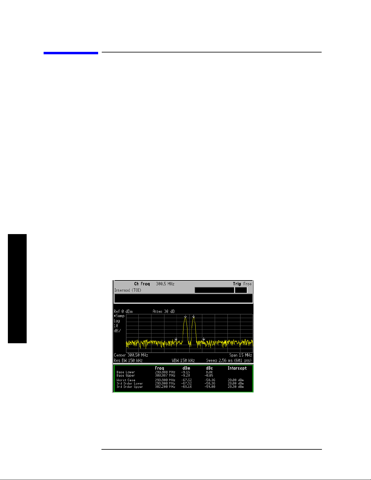
Step 3. Measure the intermodulation products using the Power Suite

Preset, Factory Preset (if present). FREQUENCY Channel, Center Freq, 300.5, MHz.

measurement tools: Press

Measure, More, Intermod (TOI).

Figure 6-5 Measuring the Distortion Products with Power Suite

Making Distortion Measurements

44 Chapter 6

Measuring Harmonics and Harmonic Distortion with a One-Button

Measuring Harmonics and Harmonic Distortion with a One-Button Measurement

This procedure measures the harmonics of the 10 MHz reference output signal. The harmonics and total harmonic distortion are measured using the one-button automated harmonic measurement.

Step 1. Preset the an alyzer:

Making Distortion Measurements

Measurement

Press

Step 2. Connect the ESA 10 MHz reference output from the rear of the

Preset, Factory Preset (if present).

analyzer to the INPUT. For PSA turn the internal 10 MHz reference signal on:

(PSA) Press

Step 3. Set the analyzer reference level, center frequency and RBW:

Press Press Press

Step 4. Run the Power Suite harmonic dis tortion measurement:

Press

Step 5. Set the number of harmonic distortion measurement averages to 3:

Press

Step 6.

Set the average mode to exponential to continuously update the result

AMPLITUDE Y Scale, Ref Level, 10, dBm. FREQUENCY Channel, Center Freq, 10, MHz. BW/Avg, Res BW, 300, kHz.

Measure, More, Harmonic Distortion.

Meas Setup, Avg Number (On), 3, Enter

System, Reference, 10MHz Out (On ) .

after each subsequent sweep: Press

Meas Setup, Avg Mode (Exp).

Making Distortion Measurements

Repeat average mode clears the averaged result after the specified number of averages is complete.

Step 7. Optimize th e analyzer ’s dynam i c ra n g e se ttings:

Press

Step 8. Display the total harmonic distort i on:

(ESA) Press (ESA) Press

Chapter 6 45

Meas Setup, Optimize Ref Level.

View/Trace, Harmonics & THD. Trace/View, Harmonics & THD.

Making Distortion Measurements

Measuring Harmonics and Harmonic Distortion with a One-Button Measurement

Figure 6-6 Measuring the Harmonic Distortion

The amplitudes of the harmonics are listed relative to the fundamental frequency.

NOTE An asterisk (*) appearing next to the total harmonic distortion value

indicates that the ideal resolution bandwidths for one or more harmonics co u l d not be set. These harmonic s fo r w hi ch th e re so l u tion bandwidths could not be set are flagged with an asterisk beside their amplitude value. The measurement is still accurate as long as the signal has little or no modulation.

Step 9. Exit out of the harmonic distortion measurement:

Press

Making Distortion Measurements

MEASURE, Meas Off.

46 Chapter 6

7 Measuring Noise

Measuring Noise

Measuring Signal-to-Noise

Signal-to-noise is a ratio used in many communication systems as an indication of noise in a system. Typically the more signals added to a system adds to the noise level, reducing the signal-to-noise ratio making it more difficult for modulated signals to be demodulated. This measurem e n t i s al so referred to as carrier-to-noise in some communication systems.

The signal-to-noise measurement procedure below may be adapt ed to measure any signal in a system if the signal (carrier) is a di screte tone. If the signal in your system is modulated, it is necessary to modify the procedure to correctly measure the modulated signal level.

In this example the 50 MHz amplitude reference signal is used as the fundamental signal. The amplitude reference signal is assumed to be the signal of interest and the inter nal noise of the anal yzer is measur ed as the system no i se. To do this, you need to se t the input atte n u a to r such that both th e si g n a l and the noise are well within the ca li b rated region of the display.

Step 1. Preset the an alyzer:

Press

Step 2. Enable the internal 50 MHz amplitude reference signal as follows:

Preset, Factory Preset (if present).

(PSA) Press

Input/Output, Input Port, Amptd Ref.

(ESA E4401B and E4411B) Press

Input/Output, Amptd Ref (On).

(ESA E4402B, E4403B, E4404B, E4405B, E4407B and E4408B) Connect a cable from the front panel AMPTD REF OUT to the analyz er RF input: Press

Step 3. Set the center frequency, span, reference level and attenuation:

Press Press Press Press

Step 4. Place a marker on the peak of the signal and then place a delta marker

Input/Output, Amptd Ref Out (On).

FREQUENCY Channel, Center Freq, 50, MHz. SPAN X Scale, Span, 1, MHz. AMPLITUDE Y Scale, Ref Level, −10, dBm. AMPLITUDE Y Scale, Attenuation, 40, dB.

in the noise at a 200 kHz offset: Press

Press

Measuring Noise

Step 5. Turn on the marker noise function to view the signal-to-noise

48 Chapter 7

Peak Search. Marker, Delta, 200, kHz.

measurement results:

Measuring Noise

Measuring Signal-to-Noise

(ESA) Press (PSA) Press

Marker, More, Function, Marker Noise. Marker Fctn, Marker Noise.

Figure 7-1 Measuring the Signal-to-Noise

Read the si gnal-to-no ise in dB/Hz , th a t is with the noi se value determined for a 1 Hz noise bandwidth. If you wish the noise value for a different bandwidth, decrease the ratio by . For example, if the analyzer reading is

−70 dB/Hz but you have a channel bandwidth of

30 kHz:

10 log× BW()

S/N 70– dB/Hz 10 30 kHz()log×+ 25.23 dB– 30 kHz()⁄==

NOTE The display detection mode is now ave rage. If the d elta marker is c loser

than one quarter of a division aw ay from the ed ge of the respo nse to the discrete signal, the amplitude reference signal in this case, there is a potential for error in the noise measurement . See “Measuring Noise

Using the Noise Marker” on page 50.

Measuring Noise

Chapter 7 49

Measuring Noise

Measuring Noise Using the Noise Marker

This procedure uses the marker function, Marker Noise, to measure noise in a 1 Hz bandwidth. In this example the noise marker measurement is made near the 50 M Hz reference signal to illustrate the use of

Marker Noise.

Step 1.

Enable the internal 50 MHz reference signal of the analyzer: (PSA)

Press

Input/Output, Input Port, Amptd Ref.

(ESA E4401B and E4411B) Press

Input/Output, Amptd Ref (On).

(ESA E4402B, E4403B, E4404B, E4405B, E4407B and E4408B) Connect a cable from the front panel AMPTD REF OUT to the INPUT : Press

Step 2. Preset the analyzer and modify the analyzer settings:

Press Press Press Press Press

Step 3. Activate the noise marker:

(ESA) Press (PSA) Press

Input/Output, Amptd Ref Out (On).

Preset, Factory Preset (if present). FREQUENCY Channel, Center Freq, 49.98, MHz. SPAN X Scale, Span, 100, kHz. AMPLITUDE Y Scale, Ref Level, −10, dBm. AMPLITUDE Y Scale, Attenuation, 40, dB.

Marker, More, Function, Marker Noise.

Marker Fctn, Marker Noise.

Note that display detection automatically changes to “Avg”; average detection calculates the noise marker from an average value of the displayed noise. Notice that the noise marker floats between the maximum and the minimum disp layed noise points . The marker readout is in dBm (1 Hz) or dBm per unit bandwidth.

For noise po we r in a diff ere nt bandw idth, ad d . For example, for noise power in a 1 kHz bandwidth, dBm (1 kHz), add or

10 log× BW()

10 log 1000()×

30 dB to the noise marker value.

NOTE ESA average detection is available for firmware revisions A.08.00 and

later. Earlier firmware revisions earlier use sample detection for marker noise calculations.

Step 4. Reduce the variations of the sweep-to-sweep marker value by

increasing the sweep time:

Measuring Noise

Press

50 Chapter 7

Sweep, Sweep Time, 3, s.

Measuring Noise Using the Noise Marker

Increasing the sweep time when the average detector is enabled allows the trace to average over a longer time interv al, thus reducing the variations in the results (increases measure ment repeatability).

Step 5. Move the marker to 50 MHz (left display Figure 7-2):

Measuring Noise

Press

Marker.

Rotate the front-panel knob until the noise marker reads 50 MHz. The noise marker value is based on the mean of 5% of the total number

of sweep points centered at the marker. The points that are averaged span one-half of a division. Notice that the marker does not go to the peak of the signal because there are not enough points at the peak of the signal. The noise marker is also averaging points below the peak due to the narrow RBW.

Step 6. Widen the resolution bandwidth to allow the marker to make a more

accurate pe ak power meas u r ement using th e no i se marker: Press

Press

BW/Avg, Res BW, 10, kHz. Marker.

Figure 7-2 Noise Marker (Left - ESA 1 kHz RBW, Right - PSA 10 kHz RBW))

Step 7. Set the analyzer to zero span at the marker frequency :

Press Press Press

Mkr →, Mkr → CF. SPAN X Scale, Zero Span. Marker.

Note that the marker amplitude value is now correct since all points averaged are at the same frequency and not influenced by the shape of the bandwidth filter.

Remember that the noise marker calculates a value based on an average of the points around the frequency of interest. Generally when making power measurements using the noise marker on discrete signals, firs t tune to the frequency of interest and then make your measurement in zero span (time-domain).

Chapter 7 51

Measuring Noise

Measuring Noise-Like Signals Using Marker Pairs

Marker pairs let you measure power over a frequency span. The markers allow you to easily and conveniently select any arbitrary portion of the displayed signal. However, while the analyzer, when autocoupled, makes sure the analysis is power-responding (rms voltage-responding), you must set all of the other parameters.

Step 1. Preset the an alyzer:

Press

Step 2. Set the center frequency, span, reference level and attenuation:

Press Press Press Press

Step 3. Turn on the marker span pair to setup the band power measureme nt in

Preset, Factory Preset (if present).

FREQUENCY Channel, Center Freq, 50, MHz. SPAN X Scale, Span, 100, kHz. AMPLITUDE Y Scale, Ref Level, −20, dBm. AMPLITUDE Y Scale, Attenuation, 40, dB.

step 5: Press

Step 4. Set the resolution and video bandwidths :

Press Press

Marker, Span Pair, Span Pair (Span), 40, kHz.

BW/Avg, Res BW, 1, kHz. BW/Avg, Video BW, 10, kHz.

Common practice is to set the resolution bandwidth from 1% to 3% of the measurement (marker) span, 40 kHz in this example. For ESA, the video bandwidth should be at least ten times wider than the resolution bandwidth.

Step 5. Measure the total noise power between the markers:

(ESA) (PSA)

Step 6. Add a discrete tone to see the effects on the re ading. Enable the int ernal

Marker, More, Function, Band Power.

Marker Fctn, Band/Intvl.

50 MHz amplitude reference signal of the analyzer as follows: (PSA)

Press

Input/Output, Input Port, Amptd Ref.

(ESA E4401B and E4411B) Press

Input/Output, Amptd Ref (On).

(ESA E4402B, E4403B, E4404B, E4405B, E4407B and E4408B) Connect a cable from the front panel AMPTD REF OUT to the analyz er

Measuring Noise

RF input: Press

52 Chapter 7

Input/Output, Amptd Ref Out (On).

Measuring Noise

Measuring Noise-Like Signals Using Marker Pairs

Figure 7-3 Band Power Marker Power Measurement (ESA left, PSA right)

Step 7. Set the marker span p air t o Center to move the markers (set at 40 kHz

span) around without changing the span. Use the front-panel knob to move the band power markers and note the change in the power reading:

Press

NOTE You can also use Delta Pair to set the meas urement start and stop points

Marker, Span Pair (Center), then rotate front-panel kno b.

independently.

Measuring Noise

Chapter 7 53

Measuring Noise

Measuring Noise-Like Signals Using the Channel Power Measurement

You may want to measure the total power of a noise-like signal that occupies some bandwidth. Typically, channel power measurements are used to measure the total (channel) power in a selecte d bandwidth for a modulated (noise-like) signal. Alternatively, to manually calculate the channel power for a modulated signal, use the noise ma rk er value and

10 log channel BW()×

add . However, if you are not certain of the characteristics of the signal, or if there ar e discrete spectral co mponents in the band of interest, you can use the channel power measurement. This example uses the noise of the analyzer, adds a discrete tone, and assumes a channel bandwidth of 50 kHz. If desired, a specific signal may be substituted.

Step 1. Preset the an alyzer:

Press

Step 2. Set the center frequency:

Press

Step 3. Start the chan nel power me a s u r ement:

Press

Step 4. Configur e t h e di splay to show th e c ombined spe c trum view wit h

Preset, Factory Preset (if present).

FREQUENCY Channel, Center Freq, 50, MHz.

MEASURE, Channel Power.

channel power limits (span highlighted in blue): (ESA) Press

(PSA) Press

Step 5. Turn averaging on:

Press

Step 6. Add a discrete tone to see the effects on the re ading. Enable the int ernal

Meas Setup, Avg Number (On).

View/Trace, Combined.

Trace/View, Combined.

50 MHz amplitude reference signal of the analyzer as follows: (PSA)

Press

Input/Output, Input Port, Amptd Ref.

(ESA E4401B and E4411B) Press

Input/Output, Amptd Ref (On).

(ESA E4402B, E4403B, E4404B, E4405B, E4407B and E4408B) Connect a cable from the front panel AMPTD REF OUT to the analyz er RF input: Press

Measuring Noise

54 Chapter 7

Input/Output, Amptd Ref Out (On).

Measuring Noise-Like Signals Using the Channel Power Measurement

Step 7. Optimize the analyzer reference level setting:

Measuring Noise

Press

Meas Setup, Optimize Ref Level.

Your display should be similar to Figure 7-4.

Figure 7-4 Measuring Channel Power (ESA left, PSA right)

The power reading is essentially that of the tone; that is, the total nois e power is far enough below that of the tone that the noise power contributes very little to the tot al.

The algorithm that computes the total power works equally well for signals of any statistical variant, whether tone-like, noise-like, or combination.

Chapter 7 55

Measuring Noise

Measuring Noise-Like Signals Using the Channel Power Measurement

Measuring Noise

56 Chapter 7

Making Time-Gated Measurements

8 Making Time-Gated

Measurements

Making Time-Gated Measurements

Generating a Pulsed-RF FM Signal

Traditional frequency-domain spectr um analysis pr ovides only limited information for certain signals. Examples of these difficult-to-analyze signal include the following:

• Pulsed-RF

• Time multiplexed

• Interleaved or intermittent

• Time domain multiple access (TDMA) radio formats

• Modulated burst

The time gating measurement examples use a simple frequency-modulated, pulsed-RF signal. The goal is to eliminate the pulse spectrum and then view the spectrum of the FM ca rrier as if it were continually on, rather than pulsed. This reveals low-level modulation components that are hidden by the pulse spectrum.

Refer back to these first three steps to setup the pulse signal, the pulsed-RF FM signal and the oscilloscop e settings when p erforming the gated LO procedure (page 62), the gated video procedure (page 64) and gated FFT procedure (page 66).

For an instrument block diagram and instrument connections see

“Connecti n g th e I n st ru ments to Make Tim e-Gated Measu rements” on page 61.

Step 1. Setup the pulse signal with a period of 5 ms and a width of 4 ms:

There are many ways to create a pulse signal. This example demonstrates how to creat e a pulse signal us ing a puls e generator or by using the in t ernal funct i o n g e n erator in the E SG. See Table 8-1 for setup information of a pulse generator and Table 8-2 for setup information of the internal generator of the ESG . Select either the pulse generator or a second ESG to create the pulse signal. You need two ESGs if you want to use the ESG internal function generator to create a pulse signal.

Table 8-1 81100 Family Pulse Generator Settings

Period 5 ms (or pulse frequency equal to 200 Hz) Pulse width 4 ms High output level 2.5 V Waveform pulse Low output level -2.5 V Delay 0 or minimum

58 Chapter 8

Making Time-Gated Measurements

Generating a Pulsed-RF FM Signal

Table 8-2 ESG #2 Internal Function Generator (LF OUT) Settings

LF Out Source FuncGen LF Out Waveform Pulse LF Out Period 5 ms

Making Time-Gated Measurements

LF Out Width (pulse width)

LF Out Amplitude 2.5 Vp LF Out On RF On/Off Off Mod On/Off On

4 ms

Step 2. Set up ESG #1 to transmit a pulsed-RF signal with frequency

modulation . Set the FM devi a ti o n to 1 kHz and the FM rate to 50 kHz: ESG #1 generates the pulsed FM signal by frequency modulating the

carrier signa l a n d then pulse modul a ti n g t he F M si gn a l . T h e pu l s e signal created in step 1 is connect ed to the EXT 2 INPUT (on the front of ESG #1). The ESG RF OUTPUT is the puls e d -R F F M sign a l to be analyzed by the spectrum analyzer.

Table 8-3 ESG #1 Instrument Connections

Frequency 40 MHz Amplitude 0 dBm Pulse On Pulse Source Ext2 DC FM On FM Path 1 FM Dev 1 kHz FM Source Internal FM Rate 50 kHz RF On/Off On Mod On/Off On

Chapter 8 59

Making Time-Gated Measurements

Generating a Pulsed-RF FM Signal

Step 3. Set up the oscilloscope to vie w the trig g er, gate and RF signals (see

Figure 8- 1 for an example of the oscilloscope display):

Table 8-4 Agilent Infiniium Oscilloscope with 3 or more input channels:

Instrument Connections

Timebase 1 ms/div

Making Time-Gated Measurements

Channel 1 ON, 2 V/div, OFFSET = 2 V, DC coupled, 1 M

connect to the pulse signal (ESG LF OUTPUT or pu ls e generator OUTPUT). Adjust channel 1 settings as necessary.

Channel 2 ON, 500 mV/div, OFFSET = 2 V, DC coupled, 1 M

input, connect to the ESA GATE/HI SWP OUT connector or PSA TRIGGER 2 OUT connector on the spectrum analyzer. Adjust channel 2 settings as needed when gate is active.

Channel 3 ON, 500 mV/div, OFFSET = 0 V, DC coupled, 50

input, connect to the ESG RF OUTPUT pulsed-RF

signal. Adjust channel 3 settings as necessary. Channel 4 OFF Trigger Edge, channel 1, level = 1.5 V, or as needed

Figure 8-1 Viewing the Gate Timing with an Oscilloscope

Ω input,

Ω

Figure 8- 1 oscilloscope channels:

1. Channel 1 (left display, top trace) - the trigger signal.

2. Channe l 2 (lef t displa y, bottom trace) - the gate signal (gate s ignal is not be activ e un t il th e gate is on in th e s pe ctrum analyzer).

3. Channel 3 (right display) - the RF output of the signal generator.

60 Chapter 8

Making Time-Gated Measurements

Connecting the Instruments to Make Time-Gated Measurements

Figure 8- 2 shows a block diagram of the test setup. ESG #1 produces a

pulsed FM signal by using an external pulse signal. The external pulse signal is connected to the front of the ESG #1 to the EXT 2 INPUT to control the pulsing. The pulse signal is also used as the trigger signal. The oscillo scope is usefu l f o r il l u strating timing intera ctions betw e en the trigger signal and the gate. PSA the oscilloscope.

Using this measurement setup allows you to view all signal spectra on the spectrum analyzer and all timing signals on the oscilloscope. This setup is helpful when you perform gated measurements on unknown signals.

Gate View could be used in place of

Making Time-Gated Measurements

Figure 8-2 Instrument Connection Diagram

Chapter 8 61

Making Time-Gated Measurements

Gated LO Measurement (PSA)

This procedure utilizes gated LO to gate the FM signal. F or conce pt and theory information about gated LO see “How Time Gating Works” on

page 135.

Step 1. Set the PSA center frequency, span and reference level:

Press Press Press

FREQUENCY Channel, Center Freq, 40, MHz. SPAN X Scale, Span, 500, kHz. AMPLITUDE Y Scale, Ref Level, −15, dBm.

In Figure 8-4 (left), the moving signals ar e a resul t of the puls ed signal. Using delta markers with a time readout, notice that the period of the spikes is at 5 ms (the same period as the pulse signal). Using time gating, these signals are be blocked out, leaving the original FM signal.

Step 2. Set the gate source to the rear external trigger input:

Press

Sweep, Gate Setup, Gate Source, Ext Rear.

Step 3. Set the gate delay to 2 ms and the gate length to 1 ms. Check that the

gate trigger is set to positive: Press

Press

Sweep, Gate Setup, Delay, 2, ms. Sweep, Gate Setup, Length, 1, ms.

Press Sweep, Gate Setup, Polarity (Pos).

Step 4. Use the PSA gate view display to confirm the gate “on” time is during

the RF burst interval (alternatively you could also use the oscilloscope to view the gate settings):

Press

Sweep, Gate Setup, Gate View (On).

Figure 8-3 Viewing the PSA Gate Settings with Gated LO

In Figure 8-3 the gray vertical line (the far left line outside of the RF envelope) represents the location equivalent to a zero gate delay.

62 Chapter 8

Making Time-Gated Measurements

Gated LO Measurement (PSA)

In Figure 8-3 the vertical green parallel bars represent the gate settings. The firs t (l e ft) bar is set at the de l ay ti m e w h il e th e s ec o n d (right) bar is set at the gate length, measured from the first bar. The trace of the signal in this time-domain view is the RF envelope. The gate signal is triggered off of the positive edge of the trigger signal.

When positioning the gate, a good starting point is to have it extend from 20% to 80% of the way through the pulse (for the PSA with linear-phase RBW filters).

While gate view mode is on, move the gate delay, length and polarity around. Notice the changes in t he vertical gate bars while making your changes. Set the gate delay, length and polarity back to the step 3 settings.

NOTE The PSA time gate triggering mode uses positive and negative edge

triggering. Level triggering is not available .

Making Time-Gated Measurements

Step 5. Turn the gate view off and enable the gate settings (see the right-side

display in Figu r e 8 - 4 ): Press

Press

Sweep, Gate Setup, Gate View (Off). Sweep, Gate (On).

Figure 8-4 Pulsed-RF FM Signal (Left), Gated FM Signal (Right)

Step 6. Turn off the pul se modulati on on ESG #1 by pressing

Pulse, Pulse so

that Off is selected. Notice that the gated spectrum is much cleaner than the ungated

spectrum (as seen in Figure 8-4). The spectrum you see with the gate on is the same as a frequency modulated signal without being pulsed. The displayed spectrum doe s not c h ang e and in both cases, you can see the two low-level modulation sidebands caused by the narrow-band FM.

Chapter 8 63

Making Time-Gated Measurements

Gated Video Measurement (ESA)

This procedure utilizes gated video to gate the FM signal. For concept and theory information about gated video see “How Time Gating

Works” on page 135.

Step 1. Set the ESA center frequency, span and reference level:

Press Press Press

FREQUENCY Channel, Center Freq, 40, MHz. SPAN X Scale, Span, 500, kHz. AMPLITUDE Y Scale, Ref Level, 0, dBm.

Step 2. Set analyzer sweep time to 2005 ms:

Press

Sweep, Sweep Time, 2005, ms.

For gated video, the calcula t ed sweep time sh o u l d b e se t to at least

# sweep points PRI (pulse repetition interval×)

to ensure that the gate is on at least once during each of the 401 sweep points. In this example, the PRI is 5 ms, so you should set the sweep time to 401 times 5 ms, or 2005 ms. If the sweep time is set too fast, some trace points may show values of zero power or other incorrect low readings. If the trace seems incomple te or erratic, try a longer sweep time.

NOTE Good practices for determining the minimum sweep time for

gated video:

In the event that the signal is not noisy, the sweep time can be set to less than (as calculated above).

# sweep points PRI (pulse repetition interval×)

Instead of using PRI in the previous sweep time calculation, we can use the “gate off time” where sweep time equals . In

# sweep points gate off time ×

our example we could use a sweep time of 401 points times 4 ms or

1.604 s. Increase the width of video bandwidth to improve the probability of capturing the pulse using “gate off time”. If trace points are still showing values of zero p ower, increase the sweep time by small increments until there are no more dropouts.

Figure 8-5 Viewing the Pulsed-RF FM Signal (without gating)

64 Chapter 8

Making Time-Gated Measurements

Gated Video Measurement (ESA)

Step 3. Set the gate delay to 2 ms and the gate length to 1 ms. Check that the

gate control is set to edge with a positive trigger:

Making Time-Gated Measurements

Press Press Press Press

Sweep, Gate, Gate Control (Edge). Edge Gate, Slope (Pos). Gate Delay, 2, ms. Gate Length, 1, ms.

Step 4. Turn the gate on:

Press

Sweep, Gate, Gate (On).

Figure 8-6 Viewing the FM Signal of a Pulsed RF Signal using Gated Video

Step 5. Notice that the gated spectrum is much cleaner than the ungated

spectrum (as seen in Figure 8-5). The spectrum you see is the same as a frequency modulated signal without being pulsed. To prove this, turn off the pulse modulation on ESG #1 by pressing is selected. The displa yed spectrum does not change.

Step 6. Check the oscilloscope display and ensure that the gate is positioned

under the pulse. The gate should be set so that it is on somewhere between 25% to 80% of the pulse. If necessary, adjust gate length and gate delay. Figure 8-7 shows the oscilloscope display when the gate is positioned correctly (the bottom trace).

Figure 8-7 The Oscilloscope Display

Pulse, Pulse so that Off

Chapter 8 65

Making Time-Gated Measurements

Gated FFT Measurement (PSA)

This procedure utilizes gated FFT to gate the FM signal. For concept and theory information about gat ed FFT see “How Time Gating Works”

on page 135.

Step 1. Set the PSA center frequency, span and reference level:

Press Press Press

FREQUENCY Channel, Center Freq, 40, MHz. SPAN X Scale, Span, 500, kHz. AMPLITUDE Y Scale, Ref Level, −15, dBm.

Step 2. Set the trigger to the external rear trigg er input:

Press

Trig, Ext Rear.

Step 3. Select the minimum resolution bandwidth required:

Press

BW/Avg, Res BW (Auto).

The duration of the analysis required is determined by the RBW. Divide

1.83 (always constant) by 4 ms to calculate the minimum RBW. The pulse width in ou r ca se is 4 ms so we need a minimu m RBW of 458 Hz. In this case because the RBW is so narrow let the analyzer choose the RBW for the current analyzer settings (span). Check that the RBW is greater tha n 458 Hz.

With the above PSA settings , the RBW s hould be 4.7 kHz. Note that the measurement speed is faster than the gated LO example. Typically gated FFT is faster than gated LO for spans less than 10 MHz.

Vary the RBW settings and note the signal changes shape as the RBW transitions from 1 kHz to 300 Hz.

Figure 8-8 Viewing the Gated FFT Measurement Results from the PSA

NOTE If the trigger event needs to be delayed use the Trig Delay function under

Trig menu. It is recommended to apply some small amount of trigger

the delay to allow time for the pulse modulator to settle.

66 Chapter 8

Measuring Digital Communications

Signals

9 Measuring Digital

Communications Signals

Measuring Digital Communications Signals

Making Burst Power Measurements

PSA and ESA spectrum analyzers make power measurements on digital communication signals fast and repea table by providing a comprehensive suite of power-based one-button automated measurements with pre-set standards-based format setups. The automated measurements also include pass/fail func tionality that allow the user to quickly check if the signal passed the measurement.

NOTE ESA spectrum analyzer sweep times: In zero-span, ESA can sweep as

fast as 10 sweep time is 1 ms. Option AYX or B7D is recommended when faster sweep times are required.

The following example demonstrates how to make a burst power

Signals

Step 1. Using an ESG, setup a Bluetooth signal transmitting DH1 pac k ets

measurement on a Bluetooth

continuously at 2.402 GHz and to the spectrum analyzer R F INP UT.

µs with 2 poin ts d i sp layed. For 101 points, the minimu m

 signal broadcasting at 2.402 GHz.

−10 dBm and connect the RF OUTPUT

Measuring Digital Communications

Step 2. Preset the analyzer, set the analyzer center frequency to 2.402 GHz:

Press Press

Step 3. Set the analyzer radio mode to Bluetooth and check to make sure

Preset, Factory Preset (if present). FREQUENCY Channel, Center Freq, 2.402, GHz.

packet type DH1 is selected: Press

Press

Step 4. Select the burst power one-button measurement from the measure

Mode Setup, Radio Std, More, Bluetooth. Mode Setup, Radio Std Setup, Packet Type (DH1).

menu and optimize the reference level: Press

Press

Step 5. View the results of the burst power measurement using the full screen

MEASURE, More, Burst Power. Meas Setup, Optimize Ref Level.

(See Figure 9-1): Press

Display, Full Screen.

68 Chapter 9

Measuring Digital Com munications Signals

Making Burst Power Measurements

Figure 9-1 Full Screen Display of Burst Power Measurement Results

NOTE Press the Return key to exit the full sc reen display wit h o u t ch anging

any parameter values.

Step 6. Select one of the following th ree trigger method s t o captur e th e burste d

signal (RF burst is recommended, if available):

Measuring Digital Communications

Signals

Press

Trig, RF Burst.

For more information on trigger selections see “Trigger Concepts” on

page 153.

NOTE Although the trigger level allows the analyzer to detect the presence of

a burst, the time samples contri buting to the burst p ower measurement are determined by the threshold level, as described next.

Step 7. Set the relative threshold level above which the burst power

measurement is calculated: Press

Meas Setup, Threshold Lvl (Rel), −10, dB.

The burst power measurement include s all points above the threshold and no points below. The threshold level is indicated on the display by the green horizontal line (for video triggering it is the upper line). In this example, the threshold level has been set to be 10 dB below the relative level of the burst. The mean power of the burst is measured from all data above the threshold level.

Step 8. Set the burst width to measure the central 200 µs of the burst:

Press (Man),

Meas Setup, Meas Method, Measured Burst Widt h, Burst Width

200, µs.

The burst width is indicated on the screen by two vertical white lines. Manually setting the burst width allows you to make it a long time interval (to include the rising and falling edges of the burst) or to make it a short time interval, measuring a small central section of the burst.

Chapter 9 69

Measuring Digital Communications Signals

Making Burst Power Measurements

NOTE If you set the burst width manually to be wider than the screen’s

display, the vertical white lines move off the edges of the screen. This could give misleading results as only the data on the screen can be measured.

NOTE The Bluetooth standard states that power measure me n ts should be

taken over at least 20% to 80% of the duration of the burst.

Step 9. Increase the sweep time to display mo re than one burst at a time:

Press

Sweep, Sweep Time, 6200, µs (or 6.2, ms).

The screen display shows several bursts in a single sweep as in

Figure 9-2. The burst power measurement measures the mean power of

the first burst, indicated by the vertical white lines.

Signals

Measuring Digital Communications

Figure 9-2 Setting Burst Width (Left) Displaying Multiple Bursts (Right)

NOTE Although th e bu r s t power measur e m e n t still runs correctly when

several bursts are disp layed simultaneously, the timing accuracy of the measurement is degraded. For the best results (including the best trade-off between measurement variations and averaging time), it is recommended that the measurement be performed on a single burst.

70 Chapter 9

Measuring Digital Com munications Signals

Making Statistical Power Measurements (CCDF)

NOTE CCDF can be measured with ESA-E series analyzers with option AYX

or B7D and with all PSA series analyzers. Complementary cumulative distribution function (CCDF) curves

characterize a signal by providing information about how much time the signal spends at or above a given power level. The CCDF measurement shows the percentage of time a signal spends at a particular power level. Percentage is on the vertical axis and power (in dB) is on the horizontal axis.

All CDMA signals, and W-CDMA signals in particular, are characterized by high power peaks that occur infrequently. It is important that these peaks are preserved otherwise separate data channels can not be received properly. Too many peak signals can also cause spectral regrowt h. If a CDMA syst em works wel l most of the time and only fails occasionally, this can often be caused by compression of the higher peak signals.

The following example shows how to make a CCDF measurement on a W-CDMA signal broadcasting at 1.96 GHz.

Step 1. Using an ESG, setup a W-CDMA signal transmitting at 1.96 GHz and

−10 dBm. Connect the RF OUTPUT to the spectrum analyzer RF

INPUT.

Step 2. Preset the analyzer and set the center frequency to 1.96 GHz:

Press Press

Preset, Factory Preset (if present). FREQUENCY Channel, Center Freq, 1.96, GHz.

Measuring Digital Communications

Signals

Step 3. Set the analyzer radio mode to 3GPP W-CDMA as a base stati on device:

Press Press

Step 4. Select the CCDF one-button measurement from the measure menu and

Mode Setup, Radio Std, 3GPP W-CDMA. Mode Setup, Radio Std Setup, Device (BTS).

then optim i z e th e reference le v e l an d attenuatio n settings sui table for the CCDF measurement:

Press Press

Chapter 9 71

MEASURE, Power Stat CCDF. Meas Setup, Optimize Ref Level.

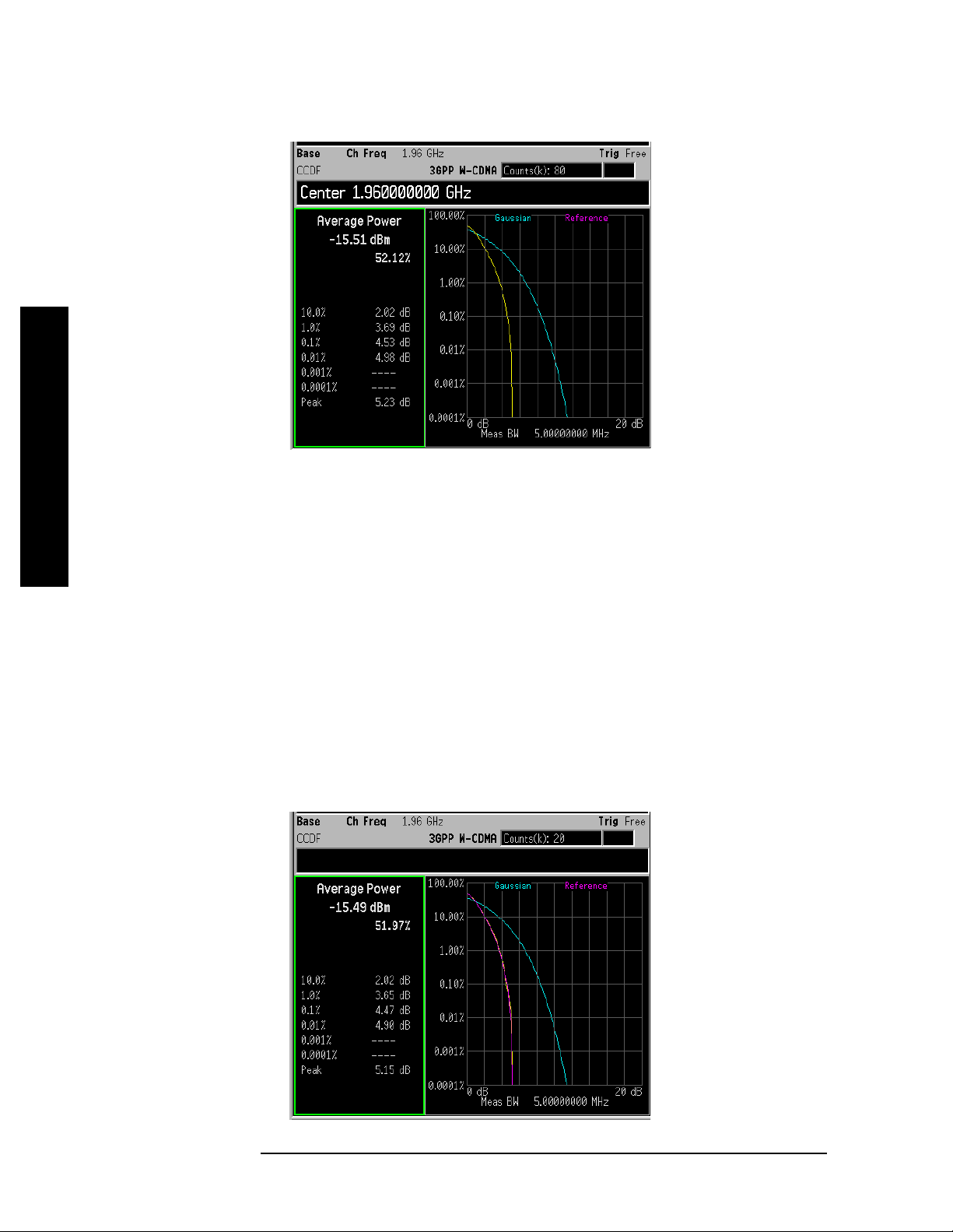
Measuring Digital Communications Signals

Making Statistical Power Measurements (CCDF)

Figure 9-3 Power Stat CCDF Measurement on a W-CDMA Signal

Signals

Step 5. Store your current measurement trace for future reference:

Press

Display, Store Ref Trace.

When the power stat CCDF measurement is first made, the graphical

Measuring Digital Communications

display should show a signal typical of pure noise. This is labelled Gaussian, and is shown in aqua. Your CCDF measurement is displayed as a yellow plot. You have stored this measurement’s plot to make for easy comparison with subsequent measurements.

Step 6. Display the stored trace:

Press

Display, Ref Trace (On).

The stored trace from your last measurement is displayed as a magenta plot (as shown in Figure 9-4), and allows direct comparison with your current measurement.

Figure 9-4 Storing and Displaying a Power Stat CCDF Measurement

72 Chapter 9

Measuring Digital Com munications Signals

Making Statistical Power Measurements (CCDF)

Step 7. Change the measurement bandwidth to 1 MHz:

Press

Meas Setup, Meas BW, 1, MHz.

Figure 9-5 Reducing the measurement ba ndwidth to 1 MHz

NOTE If you choose a measurement bandwidth setting that the analyzer

cannot displ ay, it automatically sets it se l f to th e clo se st available bandwidth setting.

Measuring Digital Communications

Signals

Step 8. Change the number of measured points from 100,000 (100k) to 1,000

(1k): Press

Meas Setup, Counts, 1, kpoints.

Reducing the number of points decreases the measurement time, however the number of points is a factor in determining measurement uncertainty and repeatability. Notice how the displayed plot loses a lot of its smoothness. You are gaining speed but reducing repeatability and increasing measurement uncertainty.

NOTE The number of points collected pe r swee p is dep enden t on the sampling

rate and the measurement interval. The number of samples that have been processed are in dicated at t he top o f the scre en. The graphical plot is continuously updated so you can see it getting smoother as measurement uncertainty is reduced and repeata bility improves.

Step 9. Change the scaling of the X-axis to 1 dB per division to optimize your

particular measurement: Press

SPAN X Scale, Scale/Div, 1, dB.

Chapter 9 73

Measuring Digital Communications Signals

Making Adjacent Channel Power (ACP) Measurements

The adjacen t ch a n n el po w e r (ACP) measu r e m e n t i s a lso referred to a s the adjacent channel power ratio (ACPR) and ad jacent channel leakage ratio (ACLR). We use the term ACP to refer to this measurement.

ACP measures the total power (rms voltage) in the specified channel and up to six pairs of offset frequencies. The measurement result reports the ratios of the offset powers to the main channel power.

The following example shows how to make an ACP measurement on a W-CDMA base station signal broadcasting at 1.96 GHz.

Step 1. Using an ESG, setup a W-CDMA signal transmitting at 1.96 GHz and

−10 dBm. Connect the RF OUTPUT to the spectrum analyzer RF

Signals

Step 2. Preset the analyzer, set the analyzer center frequency to 1.96 GHz.

INPUT.

Press Press

Measuring Digital Communications

Step 3. Set the analyzer radio mode to 3GPP W-CDMA as a base stati on device:

Press Press

Step 4. Select the adjacent channel power one-button measurement from the

Preset, Factory Preset (if present). FREQUENCY Channel, Center Freq, 1.96, GHz.

Mode Setup, Radio Std, 3GPP W-CDMA. Mode Setup, Radio Std Setup, Device (BTS).

measure menu and then optimize the reference level and attenuation settings suitable for the ACP measurement (see Figure 9-6):

Press Press

NOTE Optimize Ref Level protects against input signal overloads, but does not

MEASURE, ACP. Meas Setup, Optimize Ref Level.

necessarily set the input attenuation and reference level for optimum measurem e n t dynamic ran g e.

To improve the measurement repeatability, increase the sweep time to smooth out the trace (avera ge detecto r must be select ed). Meas urement repeatabi l it y ca n b e traded off wi th sweep time.

To increase dynamic range,

Noise Correction can be used to factor out

the added power of the noise floor effects . Noise correc tion is very useful when measuring signals near the noise floor of the analyzer.

74 Chapter 9

Measuring Digital Com munications Signals

Making Adjacent Channel Power (ACP) Measurements

Figure 9-6 ACP Measurement on a Base Station W-CDMA Signal

The frequency offsets , channel integration bandwidths, and span settings can all be modified from the default settings selected by the radio standard.

Measuring Digital Communications

Signals

Two vertical white lines indicate the bandwidth limit s of the central channel being measured.

Offsets A and B are designated by the adjacent pairs of red and yellow lines, in this case: 5 MHz and 10 MHz from the center frequency respectively.

Step 5. Select the combined spectrum and bar graph view of the results:

(ESA) Press (PSA) Press

Step 6. View the results using the full screen:

Press

NOTE Press the Return key to exit the full sc reen display wit h o u t ch anging

Display, Full Screen.

View/Trace, Combined. Trace/View, Combined.

any parameter values.

Step 7. Define a new third pair of offset frequencies:

Press

Meas Setup, Offset/Limits, Offset (C), Offset Freq (On), 15, MHz.

This third pair of offset frequencies is offset by 15.0 MHz from the center frequency (the outside offset pair) as shown in Figure 9-7. Three further pairs of offset frequencies (D, E and F) are also available.

Chapter 9 75

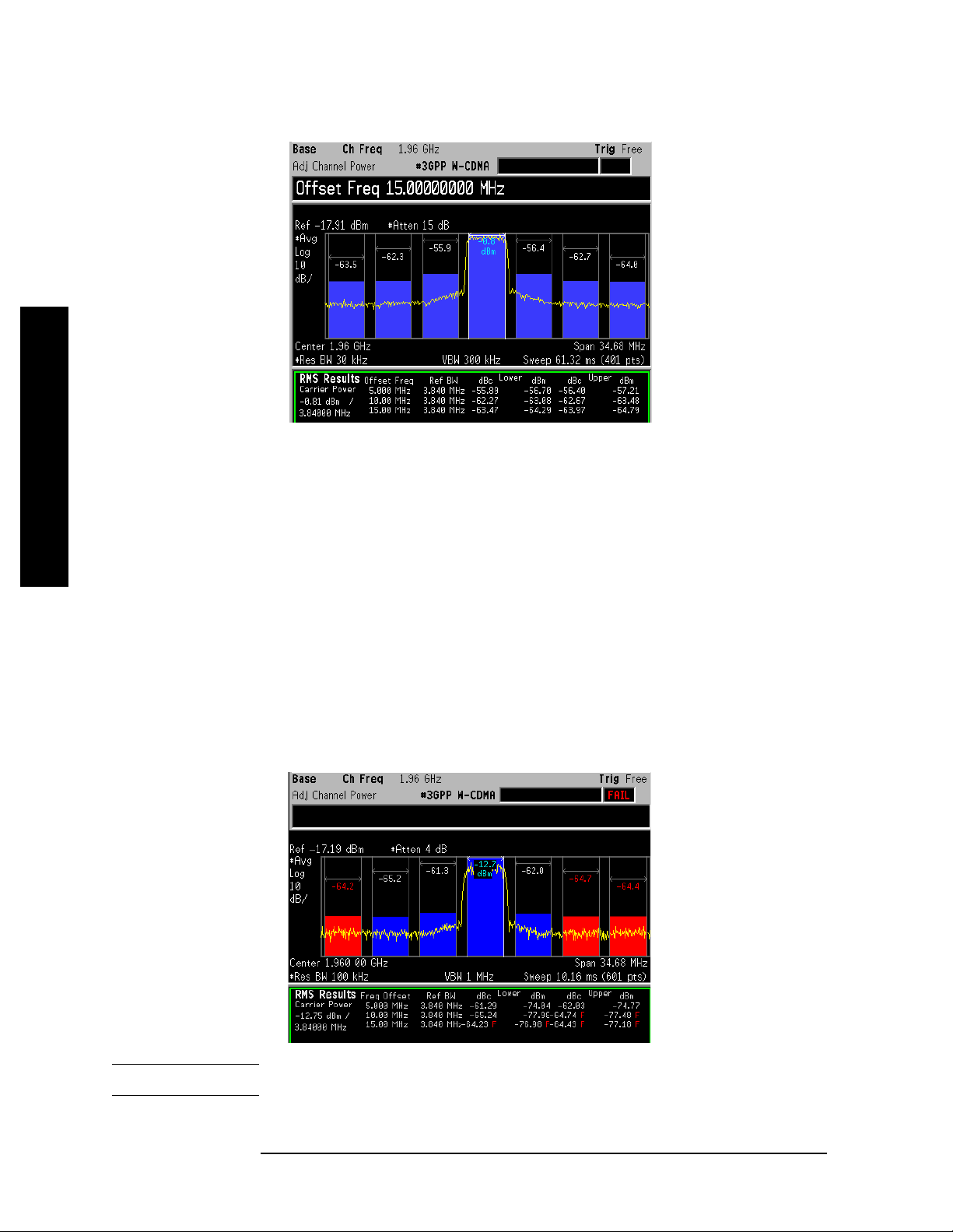
Measuring Digital Communications Signals

Making Adjacent Channel Power (ACP) Measurements

Figure 9-7 Measuring a Third Adjacent Channel

Step 8. Set pass/fail limits for each offset:

Signals

Press

Offset Limit

−65, dB, Offset (C), Neg Offset Limit, −65, dB, Pos Offset Limit, −65, dB.

Meas Setup, Offset/Limits, Offset (A), Neg Offset Limit, −55, dB, Pos

, −55, dB, Offset (B), Neg Offse t Limit, −65, dB, Pos Offset Limit,

Step 9. Turn the lim i t test on:

Measuring Digital Communications

Press

Meas Setup, More, Limit Test (On).

In Figure 9-8 notice that offset A has passed, however off sets B and C have failed. Power levels that fall below our specified

−65 dB for offsets

B and C, fail. Failures are identified by the red letter “F” next to the levels (dBc and dBm) listed in the lower portion of the window called , “RMS Results”. The offset bar graph is also shaded red to identify a failure.

Figure 9-8 Setting Offset Limits

NOTE You may increase the rep eatability by increasing the sweep time.

76 Chapter 9

Measuring Digital Com munications Signals

Making Multi-Carrier Power (MCP) Measurements

The multi-carrier power measurement measur es the total power of up to 12 carriers and their adjacent channels for up to three pairs of offset frequencies. The offset frequency properties can be modified, including the offset frequency, the integration bandwidth and upper/lower limits. The carrie r pa r a m e te rs can also be modified including carrie r w i d th , carrier integration bandwid th and whether the carrier is on or off . MCP can be setup with n o r ad i o stan da rd selected or wi th ra d i o sta n da r d settings for IS-95 and W-CDMA. Results for carriers without power present are displayed relative to the reference carrier. Results for adjacent channels are displayed in absolute power (dBm).

The following example shows how to make an MCP measurement on a W-CDMA base station broadcas ting with 8 carriers on and with two carriers off. The transmitting carriers are spaced at 5 MHz intervals at the following frequencies: 977.5 MHz, 982.5 MHz, 987.5 MHz,

992.5 MHz, 1.0075 GHz, 1.0125 GHz, 1.0175 GHz and 1.0225 GHz.

Measuring Digital Communications

Signals

NOTE Recommended equipment: The Agilent ESG signal generators can

be used to transmit W-CDMA multi-carrier signals of up to 4 carriers. The multi-carrier signal parameters can be modified inc luding channel setup, frequency offset and carrier power. An alternative way to setup multiple carriers is to use multiple ESGs, eac h transmitting one W-CDMA signal.

Step 1. Connect a W-CDMA signal with multiple carriers broadcasting at the

frequencies stated above.

Step 2. Set the center frequency of the analyzer to the midpoint of all the

carriers: Press

Press

Step 3. Set the analyzer radio mode to 3GPP W-CDMA as a base stati on device:

Press Press

Step 4. Select the multi-carrier power one-button measurement from the

Preset, Factory Preset (if present). FREQUENCY Channel, Center Freq, 1, GHz.

Mode Setup, Radio Std, 3GPP W-CDMA. Mode Setup, Radio Std Setup, Device (BTS).

measure menu and then optimize the reference level and attenuation settings suitable for the MCP measurement:

Press Press

Step 5. Set the carrier number to 10 (in our multi-carrier setup we have 8

MEASURE, Multi Carrier Power. Meas Setup, Optimize Ref Level.

carriers without 2 middle carriers):

Chapter 9 77

Measuring Digital Communications Signals

Making Multi-Carrier Power (MCP) Measurements

Press Meas Setup, Carrier Setup, Carriers, 10, Enter.

Step 6. Configure carrier 5 to have no power present:

Press

Carrier Pwr Present (No).

Step 7. Repeat step 6, configuring carrier 6 to hav e no power present. Step 8. Display the results in full screen view (see Figure 9-9):

Press

Meas Setup, Carrier Setup, Configure Carriers, Carrier, 5, Enter,

Display, Full Screen.

Figure 9-9 MCP Measurement on a Base Station W-CDMA Signal

Signals

Measuring Digital Communications

In this example, the intermodulation falls outside the transmit channels which are marked by the colored vertical lines. The white set indicates the reference car ri er. The red sets conta in th e carriers wi th power present and the blue lines mark the carriers without power present. Limits for the upp er and lower o ff sets can als o be set as s hown in the example: “Making Adjacent Channel Power (ACP)

Measurements” on page 74.

NOTE Press the Return key to exit the full sc reen display wit h o u t ch anging

any parameter values.

Step 9. View the results table of carriers 7-10:

Press

Step 10. View the results in a combined spectrum and bar graph (s ee

Meas Setup, Carrier Result, 7, Enter.

Figure 9-10):

(ESA) Press (PSA) Press

78 Chapter 9

View/Trace, Combined.

Trace/View, Combined.

Measuring Digital Com munications Signals

Making Multi-Carrier Power (MCP) Measurements

Figure 9-10 Combined Spectrum and Bar Graph View

Step 11. Save the results file to a disk.

Measuring Digital Communications

Signals

Press

File, Save, Type, More, Measurement Results, Save Now.

The results are stored in a comma separated value s format to be viewed by any personal computer spreadsheet application. All dat a shown on the display is included in this file.

Chapter 9 79

Measuring Digital Communications Signals

Making Multi-Carrier Power (MCP) Measurements

Signals

Measuring Digital Communications

80 Chapter 9

10 Using External Millimeter

Mixers (Option AYZ)

Using External Millimeter Mixers

(Option AYZ)

Using External Millimeter Mixers (Option AYZ)

Making Measurements With Agilent 11970 Series Harmonic Mixers

External harmonic mixers can be used t o extend the fre quency r ange of the E4407B, E4440A, E4446A and E4448A spec trum analyzers. Agilent Technologies manufactures external mixers that do not require biasing and cover frequency ranges from 18 GHz to 110 GHz. Fo r frequency ranges from 110 GHz up to 325 GHz, other mixers are available from other manufacturers (these mixers may require biasing). The Agilent Technologies E4407B, E4440A, E4446A, and E4448A spectrum analyzers support harmonic mixers and preselected harmonic mixers.

When using harmonic mixers, multiple mixing products are shown on the analyzer display. The output of a harmonic mixer contains the sum and difference frequencies of the in put signal with the LO and all of its harmonics. To display the correct signal, signal identification can be used to remove all undesired mixing products . Once the correct signal is identified, signal identification must be turned off to measure the amplitude accurately.

Step 1. Connect the signal sourc e and harmonic mixer to the analyzer as s hown

in Figure 10-1.

Figure 10-1 Instrument Connections with a 11970 Series Harmonic Mixer

(Option AYZ)

Using External Millimeter Mixers

CAUTION The analyzer local oscillator output power is approximately +16 dBm.

Be sure that your external harmonic mixer can accommodate the power level before connecting it to the analyzer.

NOTE Agilent 5061-5458 SMA type cables should be used t o connect the mixer

IF and LO ports to the analyzer. Do not over-tighten the cables. The maximum torque should not exceed 112 N-cm (10 in-lb.)

82 Chapter 10

Making Measurements With Agilent 11970 Series Harmonic Mixers

Step 2. Perform a factory preset:

Using External Millimeter Mixers (Option AYZ)

Press

Step 3. Set up a high frequency signal on a microwave signal generator (no

Preset, Factory Preset (if present).

modulation required). Set the frequency to 35 GHz and the amplitude to 0 dBm.

Step 4. Select external mixing, and then select band A (from 26.5 to 40 GHz):

Press Press

Input/Output, Input Mixer, Input Mixer (Ext). Ext Mix Band, 26.5−40 GHz (A).

The IF output of a harmonic mixer contains a signal at the intermediate frequency of the analyzer whenever the harmonic frequency of the LO and the frequency of the RF differ by the intermediate frequency. As a result, within a single harmonic band, a single input signal can pro d u ce m ul ti p le re sp o n se s o n the an alyzer display, only one of which is valid (see the left display in Figure 10-2). These responses come in pairs , where members of the valid response pair are separated by 642.8 MHz and either the right-most (for negative harmonics) or left-most (for posi tive harmonics) member of the pair is the correct re sponse.

Step 5. Turn on the signal identification feature to show the real s ignal

response at 35 GHz (by def au l t , th e ty p e of signal iden ti fi c a ti o n is Image Suppress):

Using External Millimeter Mixers

Press

Step 6. Place a marker on the real signal and turn off signal identification

Input/Output, Input Mixer, Signal ID (On).

before making the final amplitude measurement: Press

Press

Peak Search. Signal Ident (Off).

Figure 10-2 Signal Identification (Left - Signal Id Off; Right - Signal Id On)

(Option AYZ)

Chapter 10 83

Using External Millimeter Mixers (Option AYZ)

Setting Harmonic Mixer Bias Current

The Agilent 11970 Series harmonic mixers do not require an external bias current. Harmonic mixers that require bias can also be used. The conversion loss calibration data for mixers requiring an external bias current are most accurate when the correct bias conditions are applied.

Step 1. Before continuing, complete the previous procedure “Making

Measurements With Agilent 11970 Ser ies Harmonic Mixers” on page 82

to set up the ana l yz e r for extern a l mi x i n g in th e b an d of interest .

Step 2. Activate the bias:

Press A +I or

Step 3. Enter the desired bias current in mA.

Input/Output, Input Mixer, Mixer Config, Mixer Bias (On)

−I appears in the display annotation indicating bias is on.

The mixer bias is supplied from the IF INPUT port of the analyzer.

CAUTION The open-circuit bias voltage can be as great as ±3.5 V through a source

resistance of 500 ohms. Such voltage levels may appear when recalling an instrument state in which a bias setting has been stored.

NOTE The bias value that appears on the analyzer display is expressed in

terms of short-circuit current ( that is , the curr ent that would flow if the IF INPUT were shorted to ground). The actual current flowing in to the mixer is less.

(Option AYZ)

Using External Millimeter Mixers

84 Chapter 10

Using External Millimeter Mixers (Option AYZ)

Entering Conversion-Loss Correction Data for Harmonic Mixers

You may want to correct your measurement for the conversion-loss of the external harmonic mixer that you are using. The amplitude correction feature can be used for this.

Step 1. Access the correction factor tables for editing:

Press

AMPLITUDE Y Scale, More, Corrections, Other.

You must enter a set of amplitude correction values for the desired frequency range. Select a correction set for use with external mixing. The recommended correction set is

Step 2. Edit the conversion loss data for the mixer in use . For Agilent 11970

Other.

Series harmonic mixers and Agilent 119 74 Series pres elected harmonic mixers, these values are listed on the mixer:

Press

Edit.

The data consists of frequency/amplitude pairs. You can enter a single average value for correction over the entire fre quency band. Or you can improve frequency response accuracy by entering multiple correction points across the band. Up to 200 points may be defined for each set.

Step 3. Once the desired correction points are entered, you must turn on the

correction function to improv e dis play calibration: Press

Return, Correction (On).

Verify that the correction factors have been applied to the display data points by checking under the

Corrections menu that Apply Corrections is

set to Yes.

Using External Millimeter Mixers

(Option AYZ)

Once you have entered the correction set, save the correction set in internal memory or on floppy disk for future reference.

Chapter 10 85

Using External Millimeter Mixers (Option AYZ)

Making Measurements with Agilent 11974 Series Preselected Harmonic Mixers

Preselected mixers apply a tracking filter to the input signal before sending it to the mixer. This makes the displayed results easier to understand because it eliminates the multipl e mixing product s that are displayed using harmonic mixers (see “Making Measuremen t s With

Agilent 11970 Series Harmonic Mixers” on page 82).

Step 1. Connect the signal source and preselected mixer to the analyzer as

shown in Figure 10-3.

Figure 10-3 Instrument Connections with a Preselected Harmonic Mixer

(Option AYZ)

Step 2. Configur e t he analyzer f o r pr eselected external mi x i n g :

Using External Millimeter Mixers

Step 3. If necessary, adjust the tracking of the preselected harmonic mixer

(Presel).

Press

Input/Output, Input Mi xer, Input Mixer (Ext), Mixer Config, Mixer Type

using the procedure “Fre quency Tracking Calibration with Agilent

11974 Series Preselected Harmonic Mixers” on page 88.

Step 4. Select the desired mixing band. In this example an Agilent 11974Q (33

to 50 GH z m i x e r ) is used: Press

Step 5. Set the microwave so urce to a f requency of 40 GHz and an amplitude of

Input/Output, Input Mixer, Ext Mix Band, 33−50 GHz (Q).

−15 dBm.

Step 6. Enter the conversion-loss data for the mixer, to calibrate the amplitude

86 Chapter 10

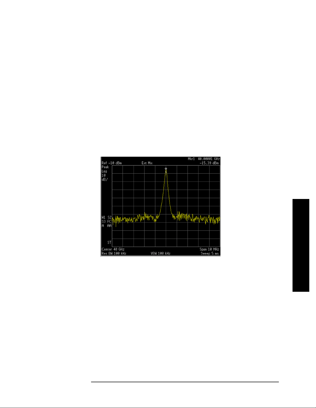
Using External Millimeter Mixers (Option AYZ)

Making Measurements with Agilent 11974 Series Preselected Harmonic

Mixers

of the display. The conversion-loss versus frequency data is on the calibration label on the bottom of the Agilent 11974, or on the supplied calibration sheet.

Use the procedure “Entering Conversion-Loss Correction Data for

Harmonic Mixers” on page 85.

Step 7. To complete the amplitude calibration process, the preselector must be

adjusted at each frequency of interest. Before making final amplitude measurements with the analyzer, perform the following:

Press Press Press

Peak Search. SPAN X Scale, Span Zoom, 10, MHz. AMPLITUDE Y Scale, Presel Center.

The final amplitude measurement can now be read out with a marker. See Figure 10-4.

Figure 10-4 Amplitude Reading of the Preselected Response

Using External Millimeter Mixers

(Option AYZ)

Chapter 10 87

Using External Millimeter Mixers (Option AYZ)

Frequency Tracking Calibration with Agilent 11974 Series Preselected Harmonic Mixers

This procedure is used to align the frequency of the pres elector filter of the Agilent 11974 to the tuned frequency of the analyzer. This procedure should be followed any time that the Agilent 11974 is connected to a different analyzer. The calibration should be periodically checked.

Step 1. Connect the signal source and preselected mixer to the analyzer as

shown in Figure 10-3.

Step 2. Set the Agilent 11974 rear-panel switches “Agilent 70907B” and

“LEDS” to the ON position, and the other two switches to the OFF

position, in order for the Agilent 11974 to properly scale to the tune signal of the analyzer.

Step 3. Configure the analyzer for a preselected external mixer:

Press Press

Preset, Factory Preset (if present). Input/Output, Input Mi xer, Input Mixer (Ext), Mixer Config, Mixer Type

(Presel).

Step 4. Set the desired frequency band of operati on for your mixer:

Press

Input/Output, Input Mixer, Ext Mix Band, t hen select external mixing

band (bands A, Q, U or V).

Step 5. Set the preselector adjustment to 0 MHz:

Press

Step 6. Set the analyzer to zero span:

(Option AYZ)

Step 7. Set the center frequency to the value in Table 10-1 for your mixer:

Using External Millimeter Mixers

Press

AMPLITUDE Y Scale, Presel Adjust, 0, MHz.

SPAN X Scale, Zero Span.

FREQUENCY Channel, Center Freq, frequency value.

On the rear panel of the Agilent 11974, adjust the corresponding potentiometer until one or both of the green LEDs are lit.

Table 10-1 Start Frequency Preselector Adjustment

Mixer Agilent P/N

Analyzer Center Frequency

Potentiometer

11974A 26.5 GHz “26.5 GHz Adjust” 11974Q 33.0 GHz “33.0 GHz Adjust” 11974U 40.0 GHz “40.0 GHz Adjust”

88 Chapter 10

Using External Millimeter Mixers (Option AYZ)

Frequency Tracking Calibration with Agilent 11974 Series Preselected

Table 10-1 Start Frequency Preselector Adjustment (Continued)

Harmonic Mixers

Mixer Agilent P/N

11974V 50.0 GHz “50.0 GHz Adjust”

Step 8. Change the analyzer center frequency to the value indicated in

Analyzer Center Frequency

Table 10-2 and again adjust the corresponding potentiometer on the

rear panel of the Agilent 11974 until one or both of the green LEDs are lit.

Table 10-2 Stop Frequency Preselector Adjustment

Mixer Agilent P/N

11974A 40.0 GHz “40.0 GHz Adjust” 11974Q 50.0 GHz “50.0 GHz Adjust” 11974U 60.0 GHz “60.0 GHz Adjust” 11974V 75.0 GHz “75.0 GHz Adjust”

Step 9. Repeat steps 6 and 7 until the green LEDs are lit at both frequencies.

Analyzer Center Frequency

Potentiometer

Using External Millimeter Mixers

(Option AYZ)

Chapter 10 89

Using External Millimeter Mixers (Option AYZ)

Frequency Tracking Calibration with Agilent 11974 Series Preselected Harmonic Mixers

(Option AYZ)

Using External Millimeter Mixers

90 Chapter 10

11 Demodulating AM and FM

Signals

Demodulating AM and FM Signals

Measuring the Modulation Rate of an AM Signal

This section demonstrates how to determine parameters of an AM signal, such as m od u l a ti on rate and modu l a tion index (de pth) by using frequency and time domain measurements (see the concepts chapter

“AM and FM Demodulation Co ncepts” on page 157 for more

information). Using the ESA built-in AM demodulator, you can also tune-in and listen to an AM signal (“Demodulating an AM Signal Using

the ESA Series” on page 96).

To obtain an AM signal, you can either connect a source transmitting an AM signal, or connect an antenna to the analyzer input and tune to a commercial AM broadcast statio n. For this demonst ration an RF sourc e is used to emulate an AM signal.

Step 1. Connect an Agilent ESG RF signal source to the analyzer INPUT. Set

the ESG frequency to 300 MHz and the amplitude to AM depth to 80%, the AM rate to 1 kHz and turn A M on .

−10 dBm. Set the

Step 2. Preset the an a l y z e r and then set the ce n ter frequen c y, span, RBW an d

the sweep time: Press

Press Press Press Press

Step 3. Set the y-axis units to volts:

Press

Step 4. Position the signal peak near the reference level:

Press

Step 5. Change the y-scale type to linear:

Press

Step 6. Set the analyzer in zero span to make time-domain measurements:

Press Press

Step 7. Use the video trigger to stabilize the trace:

Preset, Factory Preset (if present). FREQUENCY Channel, Center Freq, 300, MHz. SPAN X Scale, Span, 500, kHz. BW/Avg, Res BW, 30, kHz. Sweep, Sweep Time, 20, ms.

AMPLITUDE Y Scale, More, Y-Axis Units, Volts.

AMPLITUDE Y Scale, Ref Level, (rotate front-panel knob).

AMPLITUDE Y Scale, Scale Type (Lin).

SPAN X Scale, Zero Span. Sweep, Sweep Time, 5, ms.

Press

Trig, Video.

Since the modulation is a steady tone, you can use video trigger to trigger the analyzer sweep on the waveform and stabilize the trace, much like an oscilloscope. See Figure 11-1.

Demodulating AM and FM Signals

92 Chapter 11

Demodulating AM and FM Signals

Measuring the Modulation Rate of an AM Signal

NOTE If the trigger level is set too high or too low when video trigger mode is

activated, the sweep stops. You need to adjust the trigger level up or down with the front-panel knob until the sweep begins again.

Step 8. Measure the AM rate using delta markers:

Press

Left

Peak Search, Marker, Delta, Peak Search, Next Pk Right or Next Pk

Use markers and delta markers to measure the AM rat e. Place the marker on a peak and then use a delta marker to measure the time difference between the peaks (this is the AM rate of the signal)

NOTE Make sure the delta markers above are placed on adjacent peaks. See

Figure 11-1. The frequency or the AM rate is 1 divided by the time

between adjacent peaks: AM Rate = 1/1.0 ms = 1 kHz The spectrum analyzer can also make this rate calculation by cha nging

the marker readout to inverse time. Press Marker, More, Readout, Inverse Time.

In this example we calculated the time between time-domain peaks at the frequency of the peak of the AM signal. To make this measurement more accurately, set the center frequency to a point on the AM signal where the slope of the AM signal’s skir t is steep and then set the analyzer in zero span. Set the analyzer s weep t ime to a bout 2 times t he modulation rate and increase the number of sweep points.

Another way to calculate the modulation rate would be to view the signal in the frequency domain and measure the delta frequency between the peak of the carrier and the first sideband.

Figure 11-1 Measuring Time Parameters

Chapter 11 93

Demodulating AM and FM Signals

Measuring the Modulation Index of an AM Signal

This procedure demonstrates how to use the spect rum analyzer as a fixed-tuned (time-domain) recei ver to meas ure the mo dulation ind ex as a percent AM value of an AM signal. Using the ESA built-in AM demodulator, you can also tune-in and listen to an AM signal (“Demodulating an AM Signal Using the ESA Series” on page 96).

Step 1. Follow steps 1 through 7 of the procedure “Measuring the Modulation

Rate of an AM Signal” on page 92.

Step 2. Turn off all markers and place the analyzer in free run trigger mode:

Press Press

Step 3. Increase the sweep tim e and d ecreas e the VBW so t hat the w a v eform is

Marker, Off. Trig, Free Run.

displayed as a flat horizontal signal: Press

Press

Step 4. Center the flat waveform at the mid-point of the y-axis and then widen

Sweep, Sweep Time, 5, s. BW/Avg, Video BW, 30, Hz.

the VBW and decrease the sweep time to display the waveform as a sine wave:

Press Press Press

Step 5. Measure the modulation index of the AM signal:

AMPLITUDE Y Scale, Ref Level. BW/Avg, Video BW, 100, kHz. Sweep, Sweep Time, 5, ms.

To measure the modulation index as % AM, read the trace as follows (see Figure 11-2 for display examples): 100% AM extends from the top graticule down to the bottom graticule. 80% AM (as in this example) is when the top of the signal is at 1 division below the top graticule and 1 division above the bottom graticule. To determine % AM of your signal count each y-axis division as 10%.

Demodulating AM and FM Signals

94 Chapter 11

Demodulating AM and FM Signals

Measuring the Modulation Index of an AM Signal

Figure 11-2 AM Signal Measured in the Time Domain

LEFT: 100% AM Signal (Modulation Index = 1) RIGHT: 80% AM Signal (Modulation Index = 0.8)

Chapter 11 95

Demodulating AM and FM Signals

Demodulating an AM Signal Using the ESA Series

The demodulation functions listed in the menu under Det/Demod allow you to demodulate and hear signal information displayed on the analyzer. Simply place a marker on a signal of i nterest , set the analyzer in zero span, activate AM demodulation, turn the speaker on, and then listen.

NOTE AM demodulation is not available on the PSA Series spectrum

analyzers.

Step 1. Perform a factory preset:

Press

Step 2. Connect an antenna to the analyzer input. Step 3. Select a frequency range on the analyzer, such as the range for AM

Preset, Factory Preset (if present).

radio broadcasts. F or exampl e, the frequency range for AM broadcasts in the United States is 550 kHz to 1650 kHz:

Press

Step 4. Place a marker on the signal of interest (see Figure 11-3):

Press

FREQUENCY, Start Freq, 550, kHz, Stop Freq, 1650, kHz.

Peak Search, Next Pk Right or Next Pk Left.

Figure 11-3 AM Broadcast Signals

Step 5. Set the frequency of the signal of interest to center frequency:

Press and

Step 6. Reduce the span to 1 MHz by using the step down key (↓) and Mkr→CF

Demodulating AM and FM Signals

96 Chapter 11

Peak Searc h, Next Pk Right or Ne x t Pk Le f t (as necessary), Marker→,

Mkr→CF.

Demodulating AM and FM Signals

Demodulating an AM Signal Using the ESA Series

multiple times, keeping the signal of interest in the center of the display until the span is 1 MHz:

Press

Step 7. Set the analyzer into time-domain with zero span:

Press

Step 8. Change the resolution bandwidth to 100 kHz:

Press

Step 9. Set the top of the signal near the top of the display by changing the

SPAN X Scale, Span, (↓), Mkr→CF.

SPAN X Scale, Zero Span.

BW/Avg, Res BW, 100, kHz.

reference level with the f r on t-panel kno b : Press

Step 10. S et the amplitude scale to linear and then re-adjust the reference level

AMPLITUDE Y Scale, rotate front -panel knob.

to keep the signal centered in the display: Press

Press

Step 11. S et the detector type to sample and turn on AM demodulatio n :

Press Press

Step 12. Listen to the demodulated AM signal (adjust the volume as necessary):

AMPLITUDE Y Scale, Scale Type (Lin). AMPLITUDE Y Scale, Ref Level, rotate fron t - pa n el knob.

Det/Demod, Detector, Sample. Det/Demod, Demod, AM.

Press

Step 13. Measure the modulation index (AM depth as a percentage):

Press Press Press

Det/Demod, Demod, Speaker (On).

Sweep Time , 5, s. BW/Avg, Video BW, 30, Hz. AMPLITUDE Y Scale, Ref Level (use the front-panel knob to adjust

the trace to the middle of the scree n). Press Press

BW/Avg, Video BW, 100, kHz. Sweep, Sweep Time, 5, ms.

The middle horizontal graticule line repre sents 0% AM; the top and bottom horizontal lines represent 100% AM.

NOTE The signal to the speaker is interrupted during retrace because the

analyzer is performing automatic alignment routines. To eliminate the interruption and clicks betwe en sweeps, turn the auto alignment function off by pressing

System, Alignments, Auto Align, Off.

Refer to the specifications fo r info rmation about ope rati ng the analyzer with the alignments turned off.

Demodulating AM and FM Signals

Chapter 11 97

Demodulating AM and FM Signals

Demodulating an FM Signal Using the ESA-E Series (Requires Option BAA)

This section demonstrates how to demodulate and listen to an FM signal using the ESA built-in FM demodulator with option BAA.

Using the ESA’s built in FM demodulator you can tune to an FM signal and view the results of the detector output as displayed in the time domain. Alternatively, the demodulated signal is also available as an audio output (to the speaker or he adphone jack) and as vi deo output (on the rear panel of the ESA).

NOTE FM demodulation is not available on the PSA Series spectrum

analyzers.

Step 1. Perform a factory preset:

Press

Step 2. Use an ESG RF source or an antenna for an FM signal to analyze. In

Preset, Factory Preset (if present).

this example an ESG is used transmitting at 300 MHz with FM deviation of 10 kHz and FM rate of 1 kHz.

NOTE If you are using a broadcast FM signal in the United States, for

example, the FM channels are broadcasting between 87.7 MHz to

107.7 MHz.

Step 3. Before continuing with the demodulation of the FM signal, calibrate the

demodulator: Press

Step 4. Set the center frequency to the center of the FM signal (in this case

System, Alignments, Align Now, FM demod.

300 MHz): Press

Step 5. Set the analyzer to zero span for time-domain analysis:

Press Press

FREQUENCY Channel, Center Freq, 300, MHz.

SPAN X Scale, Zero Span. Sweep, Sweep Time, 4, ms.

Step 6. Set the resolution bandwidth to capture the full bandwidth of the FM

signal. T o calculate the required bandwidth use

RBW 2 x Frequency Deviation()2 x Modulation Rate()+()=

In our case the RBW should be: (2 x 10 kHz) + (2 x 1 kHz) = 22 kHz With E SA’s 1-3-10 sequence RBW selections, choose the next highest RBW of 30 kHz:

Demodulating AM and FM Signals

98 Chapter 11

Demodulating an FM Signal Using the ESA-E Series (Requires Option BAA)

Press BW/Avg, Res BW, 30, kHz.

Step 7. Turn on the FM demodulator:

Demodulating AM and FM Signals

Press

Step 8. Change the vertical scaling:

Press

Det/Demod, Demod, FM.

AMPLITUDE Y Scale, Scale/Div, 5, kHz.

Figure 11-4 FM Demodulation (ESG FM Signal with 10 kHz Deviation)

Step 9. Calculate the FM deviation using markers with max hold and min hold

functionality (also note that each division has 5 kHz of FM deviation if you wanted to visually calculate the deviation):

Press

View/Trace, Max Hold.

Wait until the trace appears to be a flat line before continuing to the next button sequence below:

Press

Marker, Delta, View/Trace, Min Hold.

The value on the screen from the delta value of max hold and min hold is the peak-to-peak deviation value. We are interested in the average value which we can calculate by dividing the peak-to-peak value by 2. In our case it should be approximately 20 kHz/2 or 10 kHz.

Demodulating AM and FM Signals

Chapter 11 99

Demodulating AM and FM Signals

Demodulating an FM Signal Using the ESA-E Series (Requires Option BAA)

Figure 11-5 Calculating Frequency Deviation

Step 10. Take a single sweep of the demodulated signal and then calculate the

FM rate using delta markers on adjacent peaks. Change the marker readout value to inverse time for a frequency calculation of the FM rate:

Press Press Press

Next Pk Left).

Press

Marker, Off. View/Trace, Clear Write. Single, Peak Search, Marker, Delta, Peak Search, Next Pk Right (or

Marker, More, Readout, Inverse Time.

Figure 11-6 Calculating Modulation Rate

Step 11. Listen to the FM signal (first put the analyzer back into continuous

sweeping mode): Press

Press

Sweep, Sweep (Cont). Det/Demod, Demod, Speaker (On).

Adjust the volume of the internal speaker with the volume knob on the front-panel. Alternatively you can also use the headphone jack ( located below the 3.5 inch floppy disk drive).

Demodulating AM and FM Signals

100 Chapter 11

HP e4401b, 252c02b, 252c03b, 252c04b, 252c05b schematic

Specifications and Main Features

Frequently Asked Questions

User Manual

Table of Contents

1 Recommended Test Equipment

2 Measuring Multiple Signals

Comparing Signals on the Same Screen Using Marker Delta

Comparing Signals on the Same Screen Using Marker Delta Pair

Resolving Signals of Equal Amplitude

Resolving Small Signals Hidden by Large Signals

Decreasing the Frequency Span Around the Signal

Reducing Input Attenuation

Decreasing the Resolution Bandwidth

Trace Averaging

Using a Frequency Counter to Improve Frequency Resolution and Accuracy

5 Tracking Drifting Signals

Measuring a Source’s Frequency Drift

Making Distortion Measurements

Identifying Analyzer Generated Distortion

Third-Order Intermodulation Distortion

Measuring TOI Distortion with a One-Button Measurement

Measuring Harmonics and Harmonic Distortion with a One-Button Measurement

7 Measuring Noise

Measuring Signal-to-Noise

Measuring Noise Using the Noise Marker

Measuring Noise-Like Signals Using Marker Pairs

Measuring Noise-Like Signals Using the Channel Power Measurement

Making Time-Gated Measurements

Generating a Pulsed-RF FM Signal

Connecting the Instruments to Make Time-Gated Measurements

Gated LO Measurement (PSA)

Gated Video Measurement (ESA)

Gated FFT Measurement (PSA)

Making Burst Power Measurements

Making Statistical Power Measurements (CCDF)

Making Adjacent Channel Power (ACP) Measurements

Making Multi-Carrier Power (MCP) Measurements

Making Measurements With Agilent 11970 Series Harmonic Mixers

Setting Harmonic Mixer Bias Current

Entering Conversion-Loss Correction Data for Harmonic Mixers

Making Measurements with Agilent 11974 Series Preselected Harmonic Mixers

Frequency Tracking Calibration with Agilent 11974 Series Preselected Harmonic Mixers

Demodulating AM and FM Signals

Measuring the Modulation Rate of an AM Signal

Measuring the Modulation Index of an AM Signal

Demodulating an AM Signal Using the ESA Series

Demodulating an FM Signal Using the ESA-E Series (Requires Option BAA)