HP an1337 schematic

Feeling Comfortable
with Logic Analyzers

Application Note 1337

2

Contents

Introduction

Oscilloscope or Logic Analyzer? . . . . . . . . . . . . . . . . . . . . . . . . . . . .3

What Is a Logic Analyzer? . . . . . . . . . . . . . . . . . . . . . . . . . . . . . . . . .5

Timing analyzer basics . . . . . . . . . . . . . . . . . . . . . . . . . . . . . . . . .5

State analyzer basics . . . . . . . . . . . . . . . . . . . . . . . . . . . . . . . . .12

Using Digital Tools Efficiently . . . . . . . . . . . . . . . . . . . . . . . . . . . . .17

How to Connect to Your Target System . . . . . . . . . . . . . . . . . . . . . .20

Summary . . . . . . . . . . . . . . . . . . . . . . . . . . . . . . . . . . . . . . . . . . . . . .23

If you use the right tools for the job, your attempts to conquer your digital
debug challenges will be more rewarding and less time consuming.
Before you can choose the right tool, it is important to understand the
tools at your disposal and what they do best.

This application note gives you a quick overview of logic analyzer
basics. It doesn't cover many detailed measurements, but it does give
you a good idea of what a logic analyzer can do. We explore questions
like "Why should I use a logic analyzer?" and "What will a logic analyzer
do for me?"

www.agilent.com/find/logic

3

Oscilloscope or
Logic Analyzer?

When given the choice between
using a scope or a logic analyzer,
many engineers will choose an
oscilloscope. Why? Because a scope
is more familiar to most users.
However, scopes have limited
usefulness in some applications.
Depending on what you are trying
to accomplish, a logic analyzer may
yield more useful information.
Because of overlapping capabilities
between scopes and logic analyz­ers, either may be used in some
cases. How do you determine
which is better for your applica­tion? Let's review some basic
guidelines.

When to use a scope

• When you need to see small
voltage excursions on your signal

• When you need high time-interval
accuracy

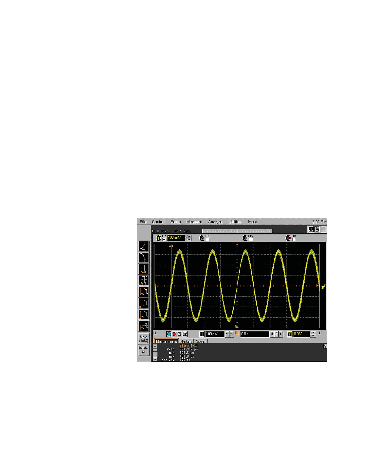
Generally, an oscilloscope is the
instrument to use when you need
high vertical or voltage resolution.
To say it another way, if you need
to see every voltage excursion, like
those shown in Figure 1, you should
use a scope.

Many scopes, including the new­generation digitizing ones, can also
provide very high time-interval
resolution. That is, they can measure
the time interval between two events
with very high accuracy. Overall, use
an oscilloscope when you need
parametric information.

Figure 1. Oscilloscope waveform

4

When to use a
logic analyzer

• When you need to see many
signals at once

• When you need to look at
signals in your system the
same way your hardware does

• When you need to trigger on a
pattern of highs and lows on
several lines and see the result

Logic analyzers grew out of
oscilloscopes. They present data
in the same general way that a
scope does: the horizontal axis is
time, the vertical axis is voltage
amplitude. But, rather than pro­viding high voltage resolution
or time-interval accuracy like a
scope, a logic analyzer can capture
and display hundreds of signals at
once, something that a scope
cannot do. A logic analyzer
reacts the same way as your
logic circuit does when a single
threshold is crossed by a signal
in your system. It recognizes the
signal to be either low or high.

It can also trigger on patterns of
highs and lows in these signals.

In general, use a logic analyzer
when you need to look at more
lines than your oscilloscope can
show you, provided you do not
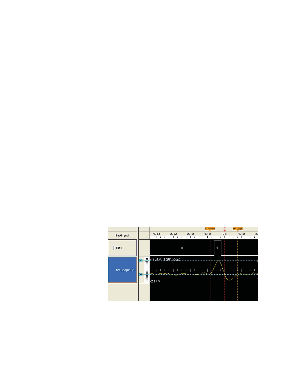
need precise time-interval infor­mation. If you need to look at
parametric information such as
rise time and fall time, a logic
analyzer is not a good choice (see
Figure 2). Logic analyzers are
particularly useful for looking
at time relationships or data on
a bus – for example, a micro­processor address, data, or
control bus. They can decode the
information on microprocessor
buses and presents it in a
meaningful form.

Generally, when you are past the
parametric stage of design, and
are interested in timing relation­ships among many signals and
need to trigger on patterns of
logic highs and lows, a logic
analyzer is the right tool.

Figure 2. Oscilloscope and timing waveforms

www.agilent.com/find/logic

5

Now that we have talked about
when to use a logic analyzer, let's
look in a bit more detail at what
a logic analyzer is. Up to now, we
have used the term "logic analyz­er" rather loosely. In fact, most
logic analyzers are really two
analyzers in one. The first part is
a timing analyzer, and the sec­ond part is a state analyzer.
Each has specific functions that
we will talk about in the follow­ing sections.

Timing analyzer basics

A timing analyzer is the part of a
logic analyzer that is analogous
to an oscilloscope. As a matter of
fact, you can think of them as
close cousins.
The timing analyzer displays
information in the same general
form as a scope, with the hori­zontal axis representing time
and the vertical axis as voltage
amplitude. Because the wave­forms on both instruments are
time-dependent, the display is
said to be in the time domain.

Choosing the right
sampling method

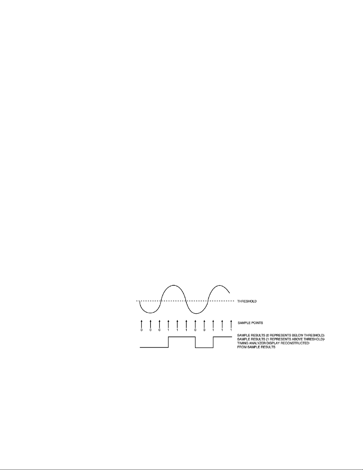
A timing analyzer works by sam­pling the input waveforms to
determine whether they are high
or low. It cares about only one
user-defined voltage-threshold. If
the signal is above the threshold
when it samples, it will be dis­played as a high or 1 by the ana­lyzer. Any signal sampled that is
below the threshold is displayed
as a 0 or low. From these sample
points, a list of ones and zeros is
generated that represents a one­bit picture of the input wave­form. As far as the analyzer is
concerned, the waveform is
either high or low – it does not
recognize intermediate steps.
This list is stored in memory and
is also used to reconstruct a one­bit picture of the input wave­form, as shown in Figure 3.

What Is a
Logic Analyzer?

Figure 3. Timing analyzer sample points

6

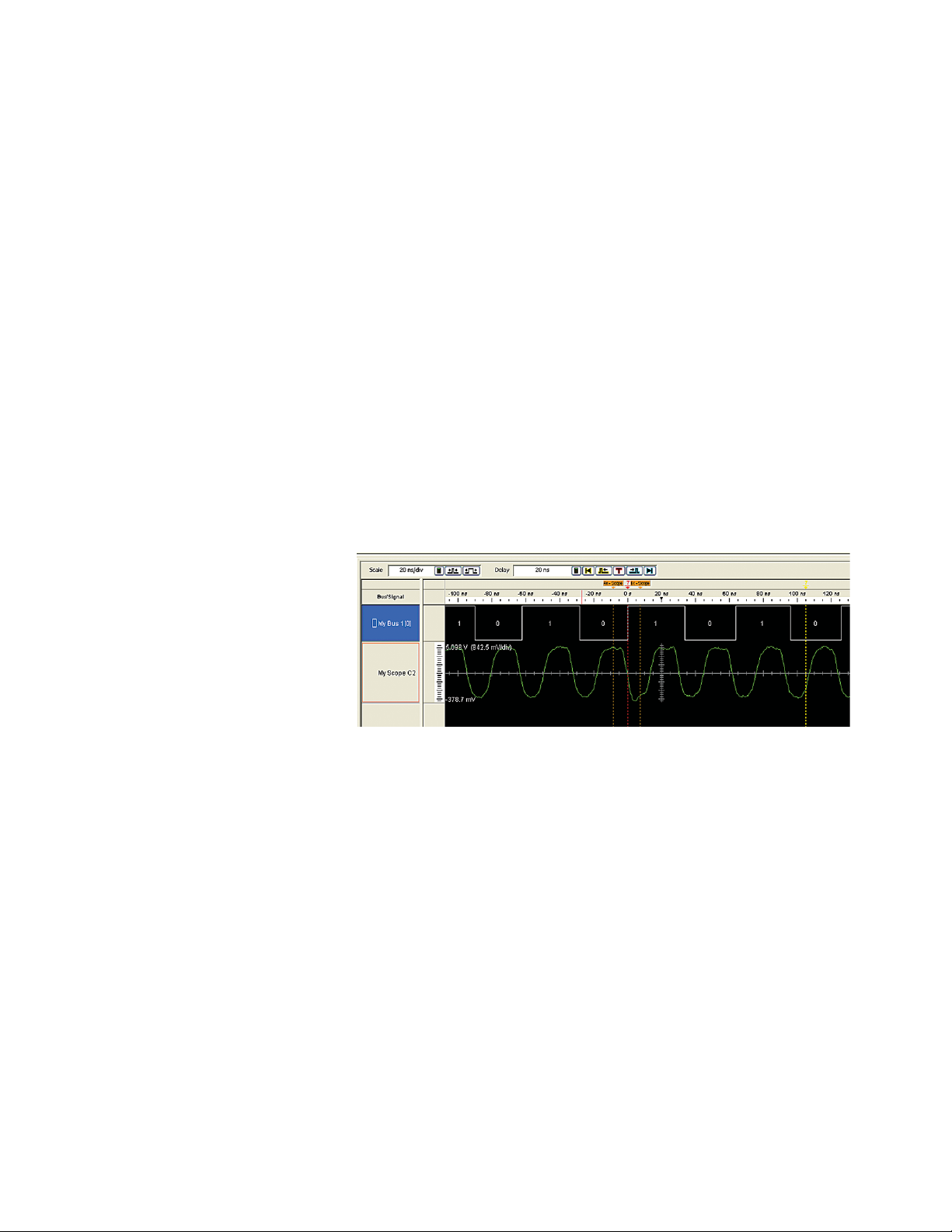
Take a look at the display shown
in Figure 4, These waveform dis­plays are actually the same sig­nal (a sine wave) displayed by a
digitizing scope and a timing
analyzer. The timing analyzer
tends to square everything up,
which would seem to limit its
usefulness. We should remember,
however, that the timing analyzer
is not intended to be a paramet­ric instrument. If you want to
check the rise time of a signal
with an analyzer, you should use
a scope. But if you need to verify
timing relationships among sev­eral or hundreds of lines by see­ing them all together, a timing
analyzer is the right choice.

For example, imagine that we
have a dynamic RAM in a system
that must be refreshed every 2
ms. To ensure that everything in
memory is refreshed within that
2 ms, a counter is used to count
up sequentially through all rows
of the RAMs and refresh each. If
we want to make certain that the
counter does indeed count up
through all rows before starting
over, a timing analyzer can be set
to trigger when the counter
starts and display all of the
counts. Parametrics are not of
great concern here – we merely
want to check that the counter
counts from 1 to N and then
starts over.

Figure 4. The same signal displayed by an oscilloscope and a timing analyzer

www.agilent.com/find/logic

7

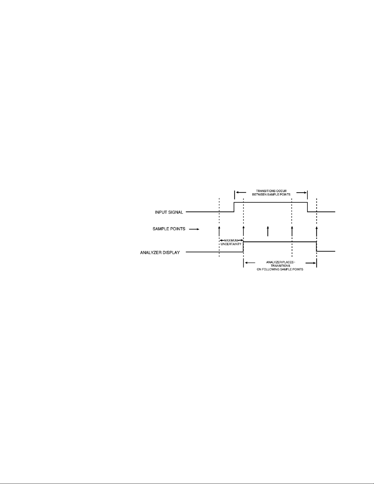
Figure 5. Timing analyzer sampling an input line

When the timing analyzer sam­ples an input line, it is either
high or low. If the line is at one
state (high or low) on one sam­ple and the opposite state on the
next sample, the analyzer
"knows" that the input signal
transitioned sometime in
between the two samples. It
doesn’t know when, so it places
the transition point at the next
sample, as shown in Figure 5.
This causes some ambiguity as to
when the transition actually
occurred and when it is dis­played by the analyzer.

The worst case for this ambiguity
is one sample period, assuming
that the transition occurred
immediately after the previous
sample point.

With this technique, however,
there is a trade-off between reso­lution and total acquisition time.
Remember that every sampling
point uses one memory location.
Thus, the higher the resolution
(faster sampling rate), the short­er the acquisition window.

8

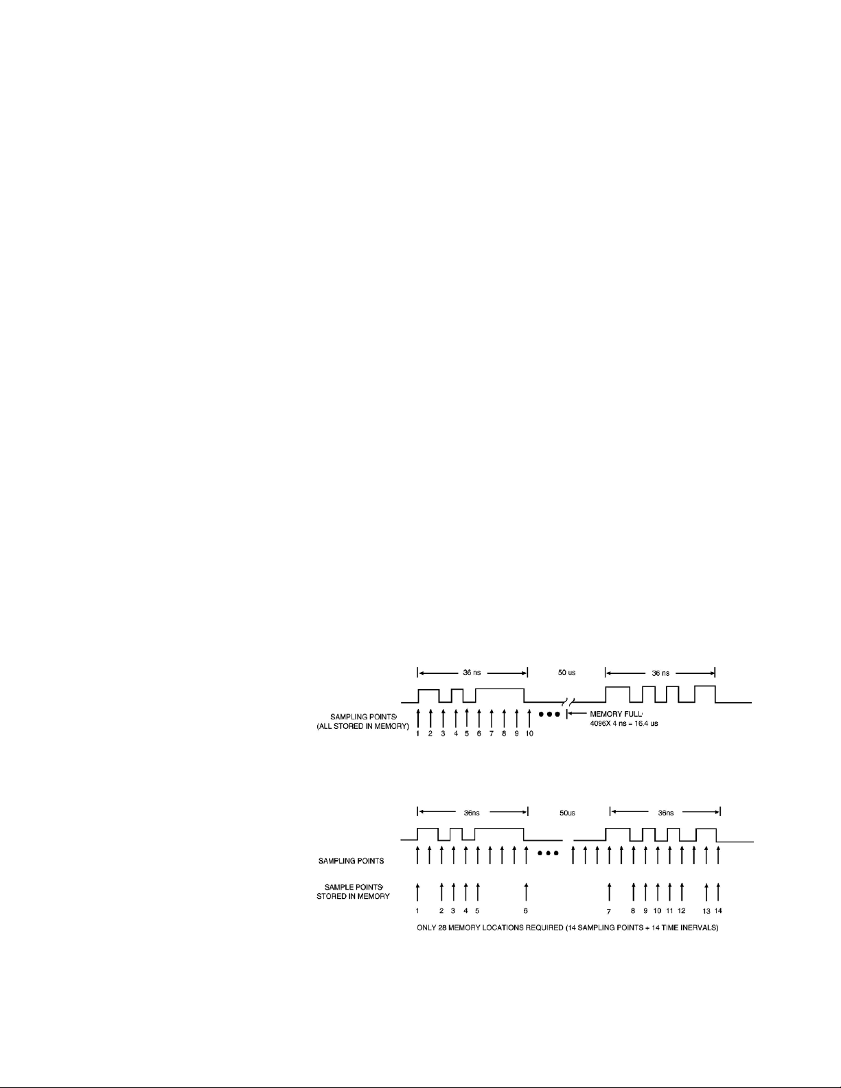
Transitional sampling

When we capture data on an
input line with data bursts, as
illustrated in Figure 6, we have to
adjust the sampling rate to high
resolution (for example, 4 ns) to
capture the fast pulses at the
beginning. This means that a
timing analyzer with 4K (4096
samples) memory would stop
acquiring data after 16.4 µs, and
you would not be able to capture
the second data burst.

Note that in our usual debugging
work we sample and store data
for a long time where there is no
activity. This uses up logic ana­lyzer memory without providing
additional information. We can
solve this problem if we know
when transitions occur and if
they are positive or negative.
This information is the basis for
transitional timing, which uses
memory efficiently.

To implement transitional timing,
we could use a “transition detector”

at the input of the timing analyzer
along with a counter. The timing
analyzer will now store only
those samples that are preceded
by a transition, together with the
elapsed time from the last transi­tion. With this approach, we use
only two memory locations per
transition and no memory at all
if there is no activity at the
input. This transitional timing
technique is used in Agilent
16800/900 Series logic analyzers.

In our example, we can capture
the second burst, and also the
third, fourth and fifth bursts,
depending on how many pulses
per burst are present. At the same
time, we can keep the timing res­olutions as high as 4 ns (Figure 7).

We can now talk about ‘effective
memory depth’, which equals the
total time data is captured divided
by the sampling period (4ns).

Note: This is a conceptual
description of the transitional
timing technique.

Figure 6. Sampling with a transition detector

Figure 7. Sampling at high resolution

www.agilent.com/find/logic

Glitch capture

Glitches in digital systems can
be problematic. Glitches have a
nasty habit of showing up at the
most inopportune times with the
most disastrous results. How do
you capture a glitch that occurs
once every 36 hours and sends
your system into the weeds?
Once again the timing analyzer
comes to the rescue. Agilent logic
analyzers have glitch capture and
trigger capability that makes it
easy to track down elusive
glitch problems.

A glitch can be caused by the
capacitive coupling between
traces, power supply ripples,
high instantaneous current
demands by several devices, or
any number of other events.
A timing analyzer samples the
incoming data and keeps track
of any transitions that occur
between samples, it can readily
recognize a glitch. In the case of
an analyzer, a glitch is defined as
any transition that crosses logic
threshold more than once
between samples. (Figure 8.)

The analyzer already keeps track
of all single transitions that occur
between samples, as we discussed
before. To recognize a glitch, we
“teach” the analyzer to keep
track of all multiple transitions
and display them as glitches.

While displaying glitches is a
useful capability, it can also be
helpful to have the ability to
trigger on a glitch and display
data that occurred before it. This
can help us to determine what
caused the glitch. This capability
also enables the analyzer to cap­ture data only when we want it –
when the glitch occurred.

Think about the example we
mentioned in the beginning para­graph of this section. We have a
system that crashes periodically
because a glitch appears on one
of the lines. Since it occurs
infrequently, to store data all the
time (assuming we had enough
storage capability) would result
in an incredible amount of infor­mation to sort through. Another
alternative is to use an analyzer
without glitch trigger capability
and sit in front of the machine
pressing the Run button and
waiting until you see the glitch.

Unfortunately, neither of the
above approaches are practical
alternatives. If we can tell the
analyzer to trigger on a glitch, it
can stop when it finds one, cap­turing all the data that happened
before it. We let the analyzer be
the babysitter, and when the
system crashes, we have a record
of what led up to the error.

9

Figure 8. A glitch

10

Triggering the timing analyzer

Another term that should be
familiar to oscilloscope users is
“triggering.” It is also used in
logic analyzers, but is often
called “trace point.” Unlike an
oscilloscope that starts the trace
right after the trigger, a logic
analyzer continuously captures
data and stops the acquisition
after the trace point is found.
Thus a logic analyzer can show
information prior to the trace
point, which is known as nega­tive time, as well as information
after the trace point.

Pattern trigger

Setting trace specifications on a
timing analyzer is a bit different
from setting trigger level and
slope on an oscilloscope. Many
analyzers trigger on a pattern of
highs and lows across input lines.

Notice the menu in Figure 9. We
have told the analyzer to start
capturing data when channels 0,
2, 4 and 6 of ‘INT4’ are high
(logical 1) and when channels
1,3,5 and 7 are low (logical 0).
Figure 10 shows the resulting
display with the line in the middle
indicating the trace point. At the
trace point channels 0, 2, 4 and 6
are all high while channels 1, 3,
5, and 7 are low.

To make things easier for some
users, the trigger point on most
analyzers can be set in binary
(1's and 0's) hex, octal, ASCII, or
decimal numbering. For instance,
to set the previous example in
hex, the trigger specification
would be 55 instead of 0101

0101. Using hex for the trigger
point is particularly helpful
when looking at buses that are
4, 8, 16, 24, or 32 bits wide.
Imagine how cumbersome it
would be to set a specification
for a 24-bit bus in binary.

Figure 9. INT4 set to trigger on a pattern of highs and lows

www.agilent.com/find/logic

11

Figure 11. Edge-triggered shift register

Figure 10. Waveform with the trace point

Edge trigger

Edge triggering is a familiar con­cept to those accustomed to
using an oscilloscope. When you
adjust the trigger level knob on a
scope, you could think of it as
setting the level of a voltage com­parator that tells the scope to
trigger when the input voltage
crosses that level. A timing ana­lyzer works essentially the same
on edge triggering except that
the trigger level is preset to logic
threshold.

Why include edge triggering in a
timing analyzer? While many
logic devices are level-dependent,
clock and control signals of these
devices are often edge-sensitive.
Edge triggering allows you to
start capturing data as the
device is clocked.

As a simple example, take the
case of an edge-triggered shift
register that is not shifting data
correctly. Is the problem with
the data or the clock edge? In
order to check the device, we
need to verify the data when it
is clocked – on the clock edge
(Figure 11).

You can tell the analyzer to cap­ture data when the clock edge
occurs (rising or falling) and
catch all of the outputs of the
shift register. Of course, in this
case we would have to delay the
trace point to take care of the
propagation delay through the
shift register.

12

State analyzer basics

In the first part of this application
note we talked about one of the
two major parts of a logic analyzer
– the timing analyzer. Next we
will talk about the other major
part of a logic analyzer – the
state analyzer.

If you’ve never used a state
analyzer, you may think it’s an
incredibly complex instrument
that would take a large time
investment to master. You might
say to yourself, “What use could
I have for a state analyzer? I
design hardware.”

The truth is many hardware
designers find a state analyzer
to be a very valuable tool, espe­cially when tracking down bugs
in software and hardware. A
state analyzer can eliminate
“finger-pointing” between hard­ware and software teams when
a problem comes up. Plus the
state analyzer is not any more
difficult to understand than the
timing analyzer.

When to use a state analyzer

If we want to understand when
to use a state analyzer, we need

to know first what a “state” is.
A “state” for a logic circuit is a
sample of a bus or line when its
data is valid.

For example, take a simple “D”
flip-flop, like the one shown in
Figure 12. Data at the “D” input
will not be valid until a positive­going clock edge comes along.
Thus, a state for the flip-flop is
when the positive clock edge occurs.

Now imagine that we have eight
of these flip-f lops in parallel. All
eight are connected to the same
clock signal (Figure 13).

When a positive transition
occurs on the clock line, all eight
will capture data at their “D”
inputs. Again, a state occurs
each time there is a positive
transition on the clock line.
These eight lines are analogous
to a microprocessor bus.

If we connected a state analyzer
to these eight lines and told it
to collect data when there is a
positive transition on the clock
line, the analyzer would do just
that. Any activity on the inputs
will not be captured by the state
analyzer unless the clock is
going high.

Figure 12. D flip-flop

Figure 13. Eight D flip-flops in parallel connected to the same clock signal

www.agilent.com/find/logic

13

Figure 14. RAM timing waveform

This points up the major differ­ence between timing and state
analyzers. The timing analyzer
has an internal clock to control
sampling, so it asynchronously
samples the system under test.
A state analyzer synchronously
samples the system since it gets its
sampling clock from the system.

As a rule of thumb, you might
remember to use a state analyzer
to check “what” happened on a
bus and a timing analyzer to see
“when” it happened. A state
analyzer generally displays data
in a listing format and a timing
analyzer displays data as a
waveform diagram. We have to
be extremely careful not to mis­interpret the data when the logic
analyzer is capable of displaying
state data as a waveform diagram
and timing data as a listing.

Understanding clocks

In the timing analyzer, sampling
is under direction of a single
internal clock. That makes things
very simple. However, in the world
of microprocessors, a system
may have several “clocks.” Let's
look at a brief example.

Suppose for a moment that we
want to trigger on a specific
address in RAM and see what
data is stored there. Further,
we'll assume that the system uses
a Zilog Z80.

In order to capture addresses
from the Z80 with our state ana­lyzer, we will want to capture
when the MREQ line goes low.
But to capture data, we will want
the analyzer to sample when the
WR line goes low (write cycle) or
when RD goes low (read cycle).
Some microprocessors multiplex
data and address on the same
lines. The analyzer must be able
to clock in information from the
same lines but different clocks.

During a read or write cycle,
the Z80 first puts an address on
the address bus. Next it asserts
MREQ, showing that the address
is valid for a memory read or
write. Last, the RD or WR line is
asserted, depending on whether
we are doing a read or write. The
WR line is asserted only after the
data on the bus is valid.

Thus, a timing analyzer acts as
a demultiplexer to capture an
address at the proper time and
then catch data that occurs on
the same lines.

14

Triggering the state analyzer

Like a timing analyzer, a state
analyzer has the capability to
qualify the data we want to store.
If we are looking for a specific
pattern of highs and lows on
the address bus, we can tell the
analyzer to start storing when it
finds the pattern and to continue
storing until the analyzer’s
memory is full. In the following
example, we have set the trigger
point as FFF03187 (hexadecimal)
(Figure 15). In this case, we want
to find out what is in location
FFF03187, so we set the data
trigger as don’t cares (XXXX).

This tells the analyzer to trigger
on address FFF03187 regardless
of what the data is at that point.

The analyzer captured address
FFF03187 and all following states.
Notice that data is 554103E7 at
address FFF03187 (Figure 16),
and that all of the information is
displayed in hexadecimal format.
We could display it in binary, if
that is helpful. However, it may
be more helpful to have the hex
decoded into assembly code.

If you specify that all information
on the buses is to be displayed in
hex, you will get a display that
resembles the one in Figure 16.

Figure 15. Trigger setup for the state analyzer

www.agilent.com/find/logic

What do these hex codes mean?
In the case of a processor, specific
hex characters comprise an
instruction. If you are very famil­iar with the hex codes, you may be
able to look at a hex listing like
the one in Figure 16 and know
what instruction it represents.
Most of us, however, can't do that.
For that reason, most analyzer
makers have designed software
packages called disassemblers or
inverse assemblers. The job of
these packages is to translate the
hex codes into assembly code to
make them easier to read.

For example, Figure 16 shows
0000 41B0 and 0000 41B1. If
we look those codes up in the
Motorola PowerQUICC manual,
we find that they represent mem
write 0x00 instructions. Rather
than having to look up each code,
the inverse assembler does it for
us. Look at Figure 17 and notice
the difference.

15

Figure 16. Data captured by the state analyzer

Figure 17. Hex codes translated into assembly code

16

Understanding sequence
levels

State analyzers have “sequence
levels” that aid triggering and
storage. Sequence levels allow
you to qualify data storage more
accurately than a single trigger
point. This means that you can
accurately window in on the data
without storing information you
don’t need. Sequence levels usu­ally look something like this:

1 find xxxx
else on xxxx go to level x 2

then find xxxx

else on xxxx go to level x 3

trigger on xxxx

Sequence levels are especially
useful for getting into a subrou­tine from a specific point in the
program.

Selective storage saves memory
and time

Sequence levels make possible
what we call selective storage.
Selective storage simply means
storing only a portion out of a
larger whole. For instance, sup­pose we have an assembly routine
that calculates the square of a
given number. If the routine is not
calculating the square correctly,
we can tell the state analyzer to
capture that routine. We do this
by first telling the analyzer to
find the start of the routine.
When it does find the start
address, we then tell it to look
for the ending address while
storing everything in-between.
When the end of the routine is
found, we tell the analyzer to
stop storing (store no states).
Figure 18 shows how selective
storage works.

Figure 18. Selective storage

Using trigger functions

Rather than defining each
sequence level from scratch,
you can use pre-defined trigger
functions. A library of common
trigger functions, such as “Find
Nth occurrence of an edge” and
“Find event ‘n’ times,” provide a
simple way to set up the analyzer
to trigger on common events and
conditions. Functions are available
for both the state and timing
acquisition modes.

You also can use pre-defined
trigger functions as a starting
point for creating custom func­tions. When you break down a
function, you gain access to all
the resource assignment fields
and branching options. You can
change these fields to change the
trigger structure.

You might need to do this to cre­ate a custom trigger specification
or to create loops and jumps in
your trigger sequence.

www.agilent.com/find/logic

17

Figure 19. Example of symptoms and cause in different domains

So far we have talked about oscil­loscopes and state and timing
analyzers and their applications.
If you are designing or servicing
digital hardware, you probably
have applications for each one of
the tools in your area. In this
section we’ll talk about how to
use these tools together to isolate
the faults in your system faster
and more efficiently.

Symptoms and their causes

If you troubleshoot digital circuitry
you often have to ask yourself,
“What causes this symptom?” It
might be quite easy to identify
the symptom of a fault, but you

need to find the cause to fix the
problem. Many times, causes
and symptoms are in different
domains. For example, a glitch
on a memory control line can
cause wrong data to be read from
or written to memory. The symp­tom (wrong data) can be found
in the data domain by using a
state analyzer and triggering on
the suspect memory address.
The cause, however, cannot be
identified in the data domain. It
is also possible that the symptom
is in the time domain (for example,
a bad handshake signal on I/O
lines), and the cause is in the
data domain (for example, wrong
software I/O routine).

Using Digital Tools
Efficiently

18

Intermodule measurements

A measurement that involves more
than one measurement instru­ment is called an “intermodule
measurement.” An intermodule
measurement requires that all
measurement tools are integrated
in a single instrument and are able
to capture data simultaneously.
Figure 20 shows the system
configuration menu from a 16800
Series logic analyzer with an
integrated oscilloscope display.
This setup provides the ability to
trace down a glitch in the oscillo­scope domain from a bad data in
the state analysis.

Cross-domain triggering

In our examples we talked about
triggering a module (state, timing
analyzer or scope) on the symptom
of the problem. Once the symptom
occurs and the appropriate ana­lyzer triggers, the module that
monitors the cause has to start
capturing data. This is achieved
by arming one module from the
trigger of the other module. For
full functionality it is necessary
that each module can receive and
send trigger signals. The bus, on
which these trigger signals are
transmitted, is called the "inter­module bus" or IMB (Figure 20).

Figure 20. System configuration menu and intermodule bus

www.agilent.com/find/logic

19

Figure 21. Setting up an intermodule measurement

Figure 22. Cross-domain measurements

Cross-domain time correlation

Once we have successfully trig­gered all our measurement mod­ules and finished data capture,
we need to look at the captured
data. We are all familiar with the
waveform display of a scope, and
we discussed how to present the
data captured by a state or tim­ing analyzer earlier. In order to
correlate from one domain to
another, it is convenient to dis­play data from both domains on
one screen. But how can we cor­relate between state and timing
other than the trace point?
Remember, the timing analyzer
uses an internal sampling clock
that is asynchronous to the sys­tem, while the state analyzer
samples synchronously to the
target system. If we count the

time between the external state
samples, we have enough time
information to correlate from
any point of the timing analyzer
waveform to the appropriate
location of the state analyzer
listing.

Application example

In Figure 22 you see the state
analyzer is used to trigger on a
certain memory access. Both the
timing analyzer and scope are
triggered by the state analyzer to
provide timing information over
multiple channels as well as
parametric information on fewer
channels. Note that the cursors
are used to correlate between
time domain (scope and timing
analyzer) and data domain
(state analyzer).

20

So far we’ve talked about some of
the differences between scopes
and timing and state analyzers.
Before we’re ready to apply
these new tools, we should talk
about one more subject – the
probing system.

From using an oscilloscope,
you're probably familiar with
passive probes. A scope probe is
designed to gain easy access to the
target system while minimizing
the signal distortion. Since we
want to look at parametric infor­mation like voltage levels and
rise times, it is important that
the probe doesn't load the circuit
under test significantly. A typical
scope probe has 1 MΩ impedance
shunted by 10 pF, depending on
the bandwidth required.

On the other hand, a logic ana­lyzer probe is designed to allow

connection of a large number of
channels to the target system
easily by trading off amplitude
accuracy of the signal under test.
Remember that a logic analyzer
only distinguishes between two
voltage levels! Traditionally, logic
analyzers used active probe pods
that had an integrated signal
detection circuitry for eight
channels capacitance, giving a
total of 16 pF per channel.

Resistive versus
capacitive loading

How does the probe impedance
affect my measurement?
Resistive and capacitive loading
are the two main cause of signal
distortion. Resistive loading
affects the amplitude of the
output through a resistive
divider effect.

How to Connect to
Your Target System

Figure 23. Resistor and capacitive loading error plot

www.agilent.com/find/logic

21

Capacitive loading affects the
timing of the signal under test by
rounding and slewing the edges.
Amplitude errors from resistive
loading are not significant
enough to affect the performance
of most circuits, even when you
are probing with 1-GHz scope
probes with 10-kΩ resistance. In
fact, most logic families can oper­ate correctly with as much as
10% error in amplitude. Because
most of these digital ICs exhibit
typical output impedance in the
low hundreds of ohms or less,
you can use a probe tip resist­ance measuring a few kΩ.

The capacitive loading of probes
becomes more important as clock
rates continue to increase in new
designs. Because of this new
increase of clock rates, circuits
are more sensitive to timing
errors of even a few nanosec­onds. The basic timing-error
immunity, on the other hand, is
limited by a circuit’s clock rate.
A CMOS circuit that drives a
given load may operate correctly
even with a higher clock rate, but
the extra capacitive loading of a
probe on that circuit can produce
unexpected timing problems.

Table 1. Increases in CMOS gate delay due to probe capacitance

Capacitance Standard CMOS delta T High-speed CMOS delta T
15 pF 25 ns 2.5 ns
8 pF 13 ns 1.3 ns
2 pF 3 ns 0.3 ns

22

Probing solutions

Physical connections to digital
systems for debugging must be
reliable and convenient to deliver
accurate data to the logic analyzer
with minimum intrusion to the
target system being debugged.
Agilent offers a broad selection
of probes and accessories for
connection to target systems.

A common probing solution is
the passive probe with sixteen
channels per cable. Each channel
is terminated at both ends with
100 kΩ and 8 pF. You can best
compare the passive probe elec­trically with the scope probe. The
advantage of the passive probing
system, besides small size and
high reliability, is that you can
terminate the probe right at the
point of connection to the target
system. This avoids additional
stray capacitance due to the
wires from the larger active pods
to the circuit under test. As a
result, your circuit under test
only "sees" 8 pF load capacitance
instead of 16 pF with previous
probing systems.

Analysis probe and other
accessories

Connecting a state analyzer to a
microprocessor system requires
some effort in terms of mechanical
connection and clock selection.
Remember, we have to clock the
state analyzer whenever data or
addresses on the bus are valid.
With some microprocessors it
might be necessary to use external
circuitry to decode several signals
to derive the clock for the state
analyzer. An analysis probe pro­vides not only fast, reliable and
correct mechanical connection to
your target system, but also the
necessary electrical adaptation
like clocking and demultiplexing
to capture your system’s
operation correctly.

Some microprocessors prefetch
information from memory that
may never get executed. Analysis
probes can also distinguish
prefetched information from exe­cuted information. Furthermore,
an analysis probe typically comes
together with a disassembler
to decode the hexadecimal infor­mation into microprocessor
mnemonics, as discussed earlier.

Figure 24. An analysis probe

www.agilent.com/find/logic

23

This application note has
explained what a logic analyzer
is and does. Since most analyzers
are made up of two major parts,
timing and state analyzers, we
have covered them separately. But
together, they make up a powerful
tool for the digital designer.

The timing analyzer is closely akin
to the oscilloscope, but is better
suited to bus-type structures or
applications where you are deal­ing with many lines. It also has
the ability to trigger on patterns
among the lines, or on glitches.

A state analyzer is most often
viewed as a software tool. In
reality, it also has many uses in
the hardware domain. Because
it gets its clock from the system
under test, it can be used to catch
data when the system sees it –
on the system's clock.

Armed with this fundamental
knowledge, you can now use a
logic analyzer with confidence
to debug your digital designs.

Related Agilent literature

• Agilent 16800 Series Portable
Logic Analyzers

Data sheet, 5989-5063EN

• Agilent 16900 Series Logic
Analysis System Mainframes

Data sheet, 5989-0421EN

For copies of this literature,
contact your Agilent representative
or visit

www.agilent.com/find/logic

Summary

Remove all doubt

Our repair and calibration services will get
your equipment back to you, performing
like new, when promised. You will get
full value out of your Agilent equipment
throughout its lifetime. Your equipment
will be serviced by Agilent-trained techni­cians using the latest factory calibration
procedures, automated repair diagnostics
and genuine parts. You will always have the
utmost confidence in your measurements.

Agilent offers a wide range of additional
expert test and measurement services for
your equipment, including initial start-up
assistance onsite education and training,
as well as design, system integration,
and project management.

For more information on repair and
calibration services, go to

www.agilent.com/find/ removealldoubt

www.agilent.com

For more information on Agilent
Technologies’ products, applications
or services, please contact your local
Agilent office. The complete list is
available at:

www.agilent.com/find/contactus

Phone or Fax

United States:

(tel) 800 829 4444
(fax) 800 829 4433

Canada:

(tel) 877 894 4414
(fax) 800 746 4866

China:

(tel) 800 810 0189
(fax) 800 820 2816

Europe:

(tel) 31 20 547 2111

Japan:

(tel) (81) 426 56 7832
(fax) (81) 426 56 7840

Korea:

(tel) [phone]
(fax) [phone]

Latin America:

(tel) [phone]

Taiwan:
(tel) 0800 047 866
(fax) 0800 286 331

Other Asia Pacific Countries:

(tel) (65) 6375 8100
(fax) (65) 6755 0042
Email: [e-mail]

Revised: 11/08/06

Product specifications and descriptions
in this document subject to change
without notice.

© Agilent Technologies, Inc. 2006
Printed in USA, December 1, 2006
5968-8291E

www.agilent.com/find/emailupdates

Get the latest information on the products
and applications you select.

www.agilent.com/find/agilentdirect

Quickly choose and use your test
equipment solutions with confidence.

www.agilent.com/find/open

Agilent Open simplifies the process of
connecting and programming test systems
to help engineers design, validate and
manufacture electronic products. Agilent
offers open connectivity for a broad range
of system-ready instruments, open industry
software, PC-standard I/O and global
support, which are combined to more
easily integrate test system development.

is the US registered trademark of

the LXI Consortium.