


Introduction
This Solutions Handbook has been designed to supplement the HP-12C Owner's
Handbook by providing a variety of applications in the financial area. Programs
and/or step-by-step keystroke procedures with corresponding examples in each
specific topic are explained. We hope that this book will serve as a reference
guide to many of your problems an d will show you how to redesign our examples
to fit your specific needs.

Real Estate
Refinancing
It can be mutually advantageous to both borrower and lender to refinance an
existing mortgage which has an interest rate substantially below the current
market rate, with a loan at a below-market rate. The borrower has the immediate
use of tax-free cash, while the lender has substantially increased debt service on
a relatively small cash outlay.
To find the benefits to both borrower and lender:
1. Calculate the monthly payment on the existing mortgage.
2. Calculate the monthly payment on the new mortgage.
3. Calculate the net monthly payment received by the lender (and paid by the borrower) by
adding the figure found in Step 1 to the figure found in Step 2.
4. Calculate the Net Present Value (NPV) to the lender of the net cash advanced.
5. Calculate the yield to the lender as an IRR.
6. Calculate the NPV to the borrower of the net cash received.
Example 1: An investment property has an existing mortgage which originated 8
years ago with an original term of 25 years, fully amortized in level monthly
payments at 6.5% interest. The current balance is $133,190.
Although the going current market interest rate is 11.5%, the lender has agreed
to refinance the property with a $200,000, 17 year, level-monthly-payment loan at
9.5% interest.
What are the NPV and effective yield to the lender on the net abount of cash
actually advanced?
What is the NPV to the borrower on this amount if he can earn a 15.25% equity
yield rate on the net proceeds of the loan?
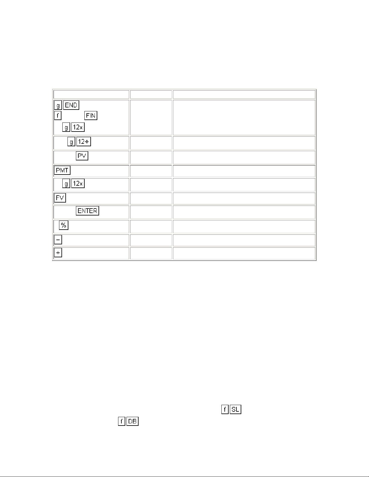
Keystrokes Display
CLEAR
17
6.5
-1,080.33
Monthly payment on existing mortgage received by
lender.
133190
0

9.5
200000
1,979.56 Monthly payment on new mortgage.
0
133190
11.5
0
0
12
15.25
0
0
899.23 Net monthly payment (to lender).
-66,810.00 Net amount of cash advanced (by lender).
-80,425.02 Present value of net
-13,615.02
14.83
-65,376.72 Present value of net monthly payment at 15.25%.
1,433.28
NPV to lender of net cash advanced
% nominal yield (IRR).
NPV to borrower.
Wrap-Around Mortgage
A wrap-around mortgage is essentially the same as a refinancing mortgage,
except that the new mortgage is granted by a different lender, who assumes the
payments on the existing mortgage, which remains in full force. The new
(second) mortgage is thus "wrapped around" the existing mortgage. The "wraparound" lender advances the net difference between the new (second) mortgage
and the existing mortgage in cash to the borrower, and receives as net cash flow,
the difference between debt service on the new (second) mortgage and debt
service on the existing mortgage.
When the terms of the origin al mortgage and the wrap-around are the same, the
procedures in calculating NPV and IRR to the lender and NPV to the borrower
are exactly the same as those presented in the preceding section on refinancing.
Example 1: A mortgage loan on an income property has a remaining balance of
$200,132.06. When the load originated 8 years ago, it had a 20-year term with
full amortization in level monthly payments at 6.75% interest.
A lender has agreed to "wrap" a $300,000 second mortgage at 10%, with full
amortization in level monthly payments over 12 years. What is the effective yield
(IRR) to the lender on the net cash advanced?
Keystrokes Display
144.00
Total number of months remaining in original load
(into n).
CLEAR
20
8
6.75
200132.06
10
300000
200132.06
12
0
0
0.56 Monthly interest rate (into i).
200,132.06 Loan amount (into PV).
-2,031.55 Monthly payment on existing mortgage (calculated).
0.83 Monthly interest on wrap-around.
-300,000.00 Amount of wrap-around (into PV).
3,585.23 Monthly payment on wrap-around (calculated).
1,553.69 Net monthly payment received (into PMT).
-99,867.94 Net cash advanced (into PV).
15.85
Nominal yield (IRR) to lender (calculated).
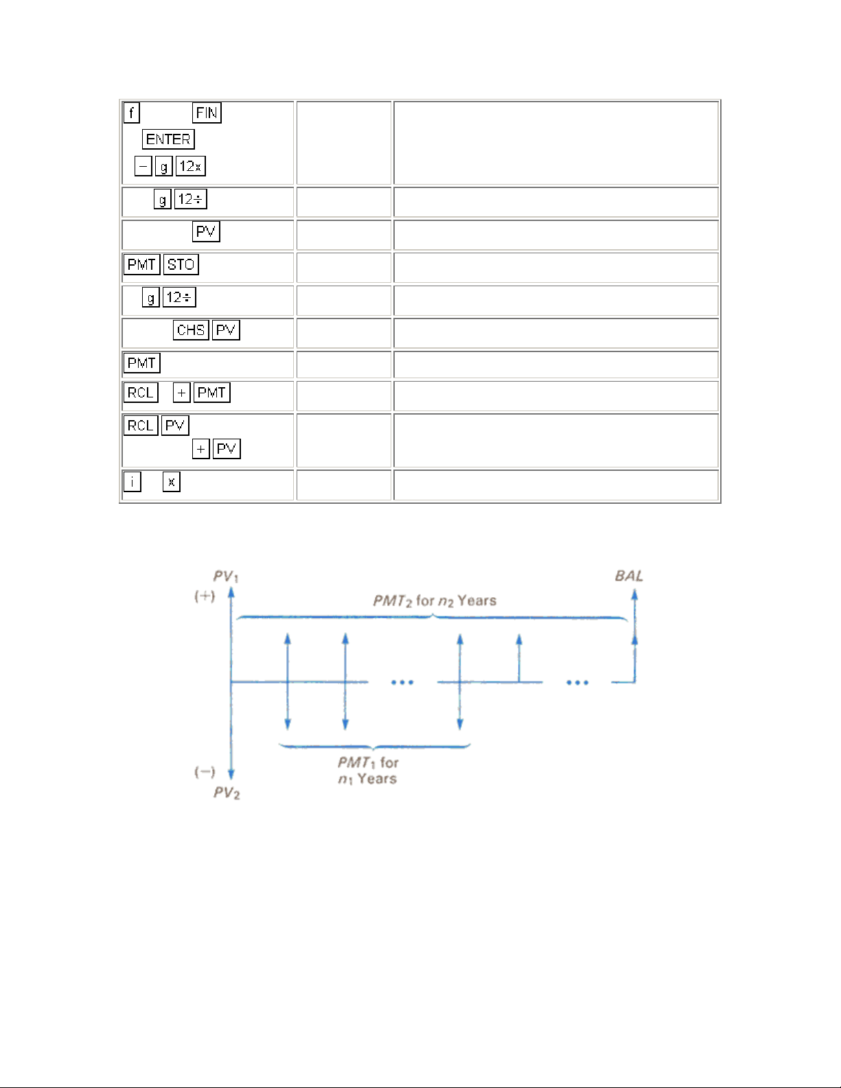
Sometimes the wrap around mortgage will have a longer payback period than the
original mortgage, or a balloon payment may exist.
where:
n1 = number of years remaining in original mortgage
PMT
= yearly payment of original m ortgage
1
= remaining balance of orig ina l m ort gage
PV
1
n
= number of years in wrap-around mortgage
2
PMT
= yearly payment of wrap-around m or tgage
2
PV
= total amount of wrap-around mortgage
2
BAL = balloon payment
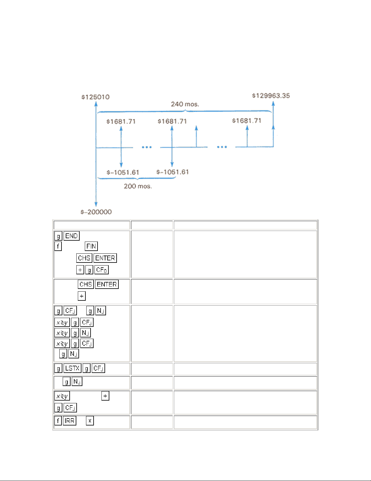
Example 2: A customer has an existing mortgage with a balance of $125.010, a
remaining term of 200 months, and a $1051.61 monthly payment. He wishes to
obtain a $200,000, 9 1/2% wrap-around with 240 monthly payments of $1681.71
and a balloon payment at the end of the 240th month of $129,963.35. If you, as a
lender, accept the proposal, what is your rate of return?
Keystrokes Display
CLEAR
200000
125010
1051.61
1681.71
2
39
99
129963.35
-74,990.00 Net investment.
630.10 Net cash flow received by lender.
The above cash flow occurs 200 times.
1,681.71 Next cash flow received by lender.
39.00 Cash flow occurs 39 times.
131,645.06 Final cash flow.
12
11.84 Rate of return to lender.
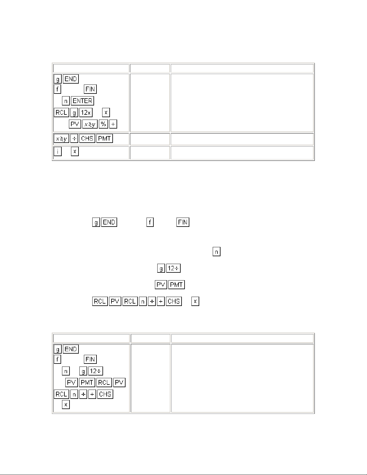
If you, as a lender, know the yield on the entire transaction, and you wish to
obtain the payment amount on the wrap-around mortgage to achieve this yield,
use the following procedure. Once the monthly payment is known, the borrower's
periodic interest rate may also be determined.
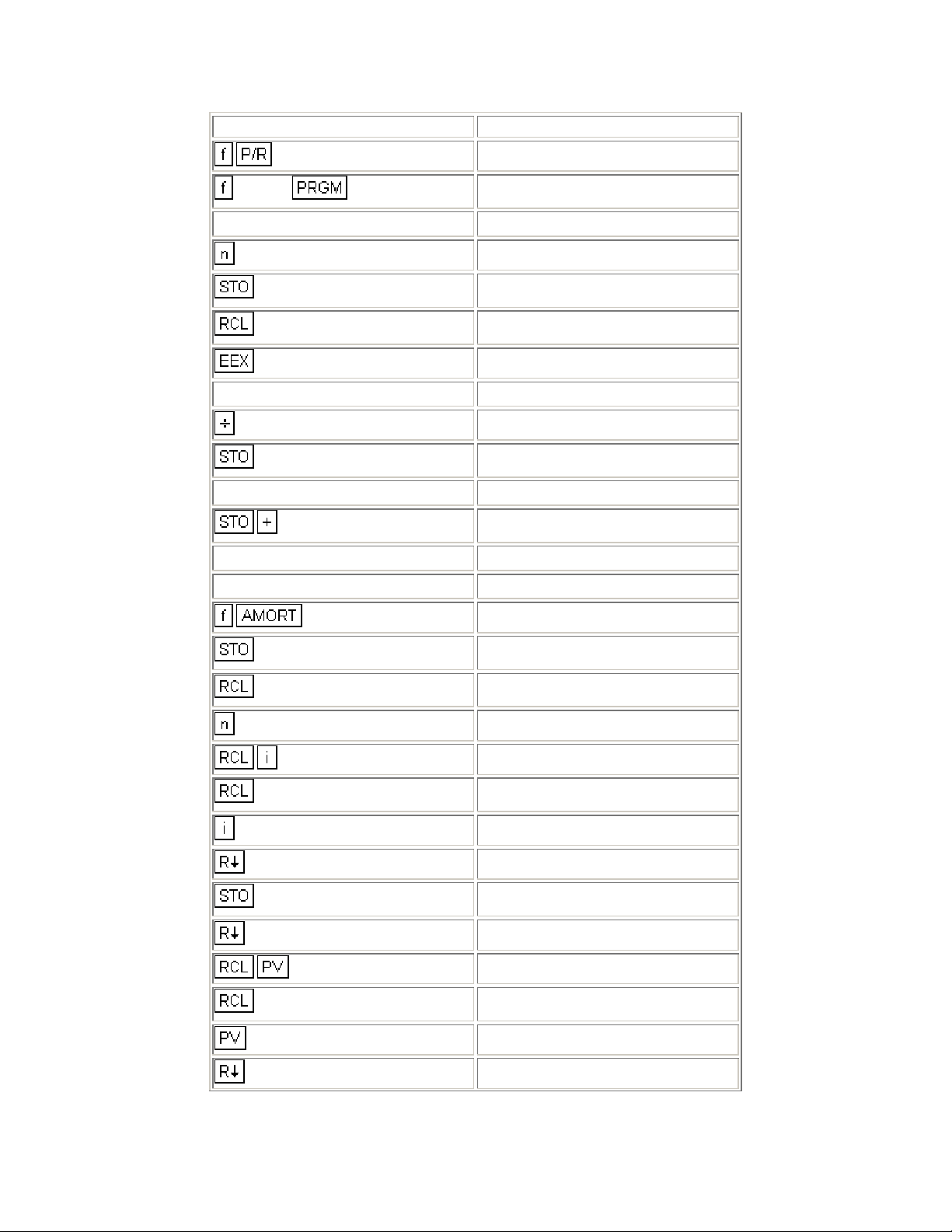
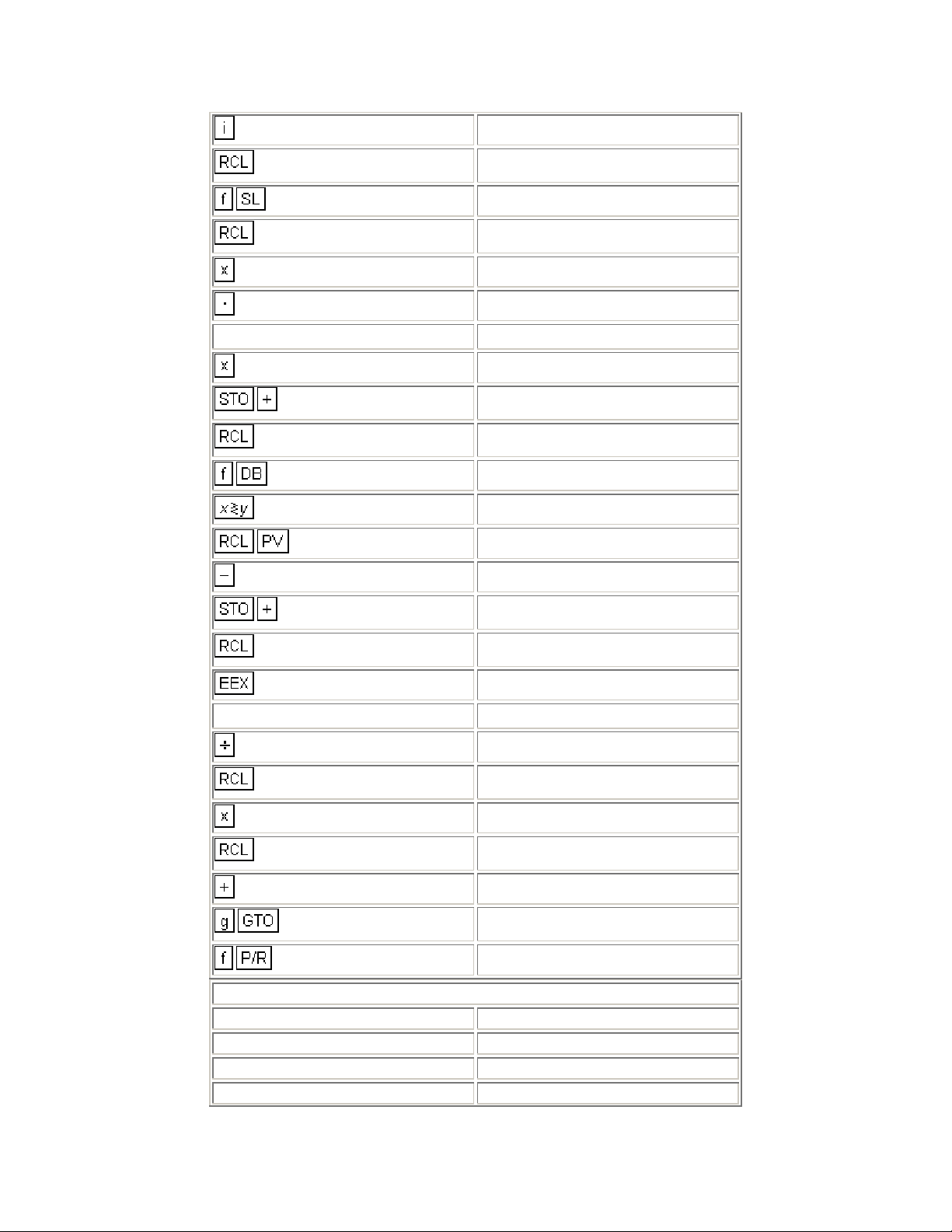
1. Press the and press CLEAR .
2. Key in the remaining periods of the original mortgage and press
3. Key in the desired annual yield and press
4. Key in the monthly payment to be made by the lender on the original mortgage and press
.
5. Press
6. Key in the net amount of cash advanced and press
7. Key in the total term of the wrap-around mortgage and press
8. If a balloon payment exists, key it in and press
9. Press
10. Key in the amount of the wrap-around mortgage and press
borrower's periodic interest rate.
.
to obtain the payment amount necessary to achieve the desired yield.
.
.
.
.
.
to obtain the
Example 3: Your firm has determined that the yield on a wrap-around mortgage
should be 12% annually. In the previous example, what monthly payment must
be received to achieve this yield on a $200,000 wrap-around? What interest rate
is the borrower paying?
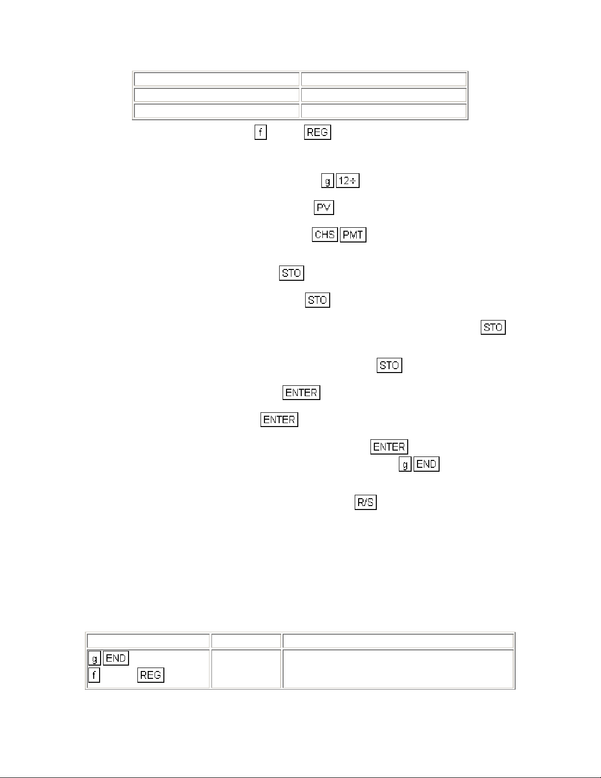
Keystrokes Display
CLEAR
200
1051.61
240
129963.35
12
74990
Number of periods and monthly interest rate.
-165,776.92 Present value of payments plus cash advanced.
1,693.97 Monthly payment received by lender
9.58 Annual interest rate paid by borrower.

12
Income Property Cash Flow Analysis
Before-Tax Cash Flows
The before-tax cash flows applicable to real estate analysis and problems are:
Potential Gross Income
•
Effective Gross Income
•
Net Operating Income (also called Net Income Before Recapture.)
•
Cash Throw-off to Equity (also called Gross Spendable Cash)
•
The derivation of these cash flows follows a set sequence:
1. Calculate Potential Gross Income by multiplying the rent per unit times the number of
units, times the number of rental payments periods per year. This gives the rental income
the property would generate if it were fully occupied.
2. Deduct Allowance for Vacancy and Rental Loss. This is usually expressed as a
percentage. The result is Rent Collections (which is also Effective Gross Income if there
is no "Other Income").
3. Add "Other Income" such as receipts from concessions (laundry equipment, etc.),
produced from sources other than the rental office space. This is Effective Gross Income.
4. Deduct Operating Expenses. These are expenditures the landlord-investor must make,
by contract or custom, to preserve the property and keep in capable of producing the
gross income. The result is the Net Operating Income.
5. Deduct Annual Debt Service on the mortgage. This produces Cash Throw-Off to Equity.
Thus:
Effective Gross Income =
Potential Gross Income - Vacancy Loss + Other Income.
Net Operating Income =
Effective Gross Income - Operating Expenses.
Cash Throw-Off =
Net Operating Income - Annual Dept Service.
Example: A 60-unit apartment building has rentals of $250 per unit per month.
With a 5% vacancy rate, the annual operating cost is $76,855.
The property has just been financed with a $700,000 mortgage, fully amortized in
a level monthly payments at 11.5% over 20 years.
a. What is he Effective Gross Income?
b. What is the Net Operating Income?
c. What is the Cash Throw-Off to Equity?
Keystrokes Display
CLEAR
60
250
5
76855
20
11.5
700000
12
12
180,000.00 Potential Gross Income.
9,000.00 Vacancy Loss.
171,000.00 Effective Gross Income.
94,145.00 Net Operating Income.
-89,580.09 Annual Debt Service.
4,564.91 Cash Throw-Off.
Before-Tax Reversions (Resale Proceeds)
The reversion receivable at the end of the income projection period is usually
based on forecast or anticipated resale of the property at that time. The beforetax reversion amount applicable to real estate analysis and problems are:
Sale Price.
•
Cash Proceeds of Resale.
•
Outstanding Mortgage Balance.
•
Net Cash Proceeds of Resale to Equity.
•
The derivation of these reversions are as follows:
1. Forecast or estimate Sales Price. Deduct sales and Transaction Costs. The result is the
Proceeds of Resale.
2. Calculate the Outstanding Balance of the Mortgage at the end of the Income Projection
Period and subtract it from Proceeds of Resale. The result is net Cash Proceeds of
Resale.
Thus:
Cash Proceeds of Resale =
Sales Price - Transaction Costs.
Net Cash Proceeds of Resale =
Cash Proceeds of Resale - Outstanding Mortgage Balance.
Example: The apartment property in the preceding example is expected to be
resold in 10 years. The anticipated resale price is $800,000. The transaction
costs are expected to be 7% of the resale price. The mortgage is the same as
that indicated in the preceding example.
What will the Mortgage Balance be in 10 years?
•
What are the Cash Proceeds of Resale and Net Cash Proceeds of Resale?
•
Keystrokes Display
CLEAR
240.00 Mortgage term.
20
11.5
700000
10
800000
7
0.96 Mortgage rate.
Property value.
-7,465.01 Monthly payment.
120.00 Projection period.
-530,956.57 Mortgage balance in 10 years.
Estimated resale.
56,000.00 Transaction costs.
744,000.00 Cash Proceeds of Resale.
213,043.43 Net Cash Proceeds of Resale.
After-Tax Cash Flows
The After-Tax Cash Flow (ATCF) is found for the each year by deducting the
Income Tax Liability for that year from the Cash Throw Off.
where:
Taxable Income =
Net Operating Income - interest - depreciation.
Tax Liability =
Taxable Income x Marginal Tax Rate.
After Tax Cash Flow =
Cash Throw Off - Tax Liability.
The After-Tax Cash Flow for the initial and successive years may be calculated
by the following HP-12C program. This program calculates the Net Operating
Income using the Potential Gross Income, operational cost and vacancy rate.
The Net Operating Income is readjusted each year from the growth rates in
Potential Gross Income and operational costs.
The user is able to change the method of finding the depreciation from declining
balance to straight line. To make the change, key in at line 32 of the
program in place of .
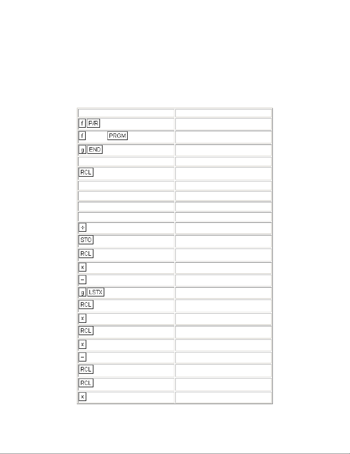
KEYSTROKES DISPLAY
CLEAR
0
1
7
2
7
1
1
1
2
0001- 0
02- 11
03- 44 1
04- 45 7
05- 26
06- 2
07- 10
08- 44 7
09- 1
10-44 40 1
11- 1
12- 2
0
5
6
6
4
13- 42 11
14- 44 0
15- 45 5
16- 11
17- 45 12
18- 45 6
19- 12
20- 33
21- 44 6
22- 33
23- 45 13
24- 45 4
25- 13
26- 33
4
27- 44 4
0
36
1
0
28- 33
29- 43 35
30-43,33 36
31- 45 1
32- 42 25
33-44 30 0
34- 0
17
2
8
2
35-43,33 17
36- 11
37- 45 2
38- 45 8
39- 25
40-44 40 2
1
0
3
9
3
41- 33
42-45 48 0
43- 25
44- 30
45- 45 3
46- 45 9
47- 25
48-44 40 3
49- 33
50- 30
51- 1
7
0
52- 45 7
53-44 20 0
54- 30
1
55- 20
56- 45 14
57- 1
2
0
1
09
REGISTERS
n: Used i: Annual %
PV: Used PMT: Monthly
FV: 0 R0: Used
R1: Counter
R3: Oper. cost R4: Dep. value
R5: Dep. life R6: Factor (DB)
R7: Tax Rate R8: % gr. (PGI)
R9: % gr. (op) R.0: Vacancy rt.
58- 2
59- 20
60- 40
61- 45 0
62- 30
63- 45 1
64- 43 31
65- 34
66- 31
67-43,33 09
R
: PGI
2
1. Press and press CLEAR .
2. Key in loan values:
Key in annual interest rate and press
•
Key in principal to be paid and press
•
Key in monthly payment and press
•
(If any of the values are not known, they should be solved for.)
3. Key in Potential Gross Income (PGI) and press
4. Key in Operational cost and press
3.
2.
5. Key in depreciable value and press 4.
6. Key in depreciable life and press
7. Key in factor (for declining balance only) and press
8. Key in the Marginal Tax Rate (as a percentage) and press
9. Key in the growth rate in Potential Gross Income ( 0 for no growth) and press
10. Key in the growth rate in operational cost (0 if no growth) and press
11. Key in the vacancy rate (0 for no vacancy rate) and press
12. Key in the desired depreciation function at line 32 in the program.
13. Press
with the ATCF for that year. The Y-register contains the year.
14. Continue pressing
to compute ATCF. The display will pause showing the year and then will stop
to compute successive After-Tax Cash Flows.
5.
6.
7.
8.
9.
0.
Example 1: A triplex was recently purchased for $100,000 with a 30-year loan at
12.25% and a 20% down payment. Not including a 5% annual vacancy rate, the
potential gross income is $9,900 with an annual growth rate of 6%. Operating
expenses are $3,291.75 with a 2.5% growth rate. The depreciable value is
$75,000 with a projected useful life of $20 years. Assuming a 125% declining
balance depreciation, what are the After-Tax Cash Flows for the first 10 years if
the investors Marginal Tax Rate is 35%?
Keystrokes Display
CLEAR
100000
20
12.25
30
9900 2
3291.75 3
75000 4
20 5
80,000.00 Mortgage amount.
1.02 Monthly interest rate.
360 Mortgage term.
-838.32 Monthly payment.
9,900.00 Potential Gross Income.
3,291.75 1st year operating cost.
75,000.00 Depreciable value.
20.00 Useful life.
125 6
125.00 Decline in balance factor.
35 7
6 8
2.5 9
5 .0
35.00 Marginal Tax Rate.
6.00 Potential Gross Income growth rate.
2.50 Operating cost growth.
5.00 Vacancy rate.
1.00
-1,020.88
2.00
-822.59
3.00
-598.85
4.00
-72.16
5.00
232.35
6.00
565.48
7.00
928.23
8.00
1,321.62
9.00
1,746.81
10.00
-1,020.88
Year 1
ATCF
1
Year 2
ATCF
2
Year 3
ATCF
3
Year 4
ATCF
4
Year 5
ATCF
5
Year 6
ATCF
6
Year 7
ATCF
7
Year 8
ATCF
8
Year 9
ATCF
9
Year 10
ATCF
10
Example 2: An office building was purchased for $1,400,000. The value of
depreciable improvements is $1,200,000.00 with a 35 year economic life.
Straight line depreciation will be used. The property is financed with a $1,050,000
loan. The terms of the loan are 9.5% interest and $9,173.81 monthly payments
for 25 years. The office building generates a Potential Gross Income of
$175,2000 which grows at a 3.5% annual rate. The operating cost is $40,296.00
with a 1.6% annual growth rate. Assuming a Marginal Tax Rate of 50% and a
vacancy rate of 7%, what are the After-Tax Cash Flows for the first 5 years?
Keystrokes Display
CLEAR
1050000
9173.81
175,200.00 Potential Gross Income.
25
175200
40296 3
1200000 4
35 5
50 7
3.5 8
1.6 9
7 0
2
31
40,296.00 1st year operating cost.
1,200,000.00 Depreciable value.
35.00 Depreciable life.
50.00 Marginal tax rate.
3.50 Potential Gross Income
1.60 Operating cost growth rate.
7.00 Vacancy rate.
7.00 Go to dep. step.
32- 42
23
1.00
18,021.07
2.00
20,014.26
3.00
22,048.90
4.00
24,123.14
5.00
26,234.69
Change to SL.
Year 1
ATCF
1
Year 2
ATCF
2
Year 3
ATCF
3
Year 4
ATCF
4
Year 5
ATCF
5
After-Tax Net Cash Proceeds of Resale
The After-Tax Net Cash Proceeds of Resale (ATNCPR) is the after-tax reversion
to equity; generally, the estimated resale price of the property less commissions,
outstanding debt and any tax claim.
The After-Tax Net Cash Proceeds can be found using the HP-12C program
which follows. In calculating the owner's income tax liability on resale, this
program assumes that the owner elects to have his capital gain taxed at 40% of
his Marginal Tax Rate. This assumption is in accordance with a 1978 Federal tax
ruling.
* (*
Federal Taxes, code sec. 1202 (32,036))
This program uses declining balance depreciation to find the amount of
depreciation from purchase to sal e. This amount is used to determine the excess
depreciation (which is equal to the amount of actual depreciation minus the
amount of the straight line depreciation).
The user may change to a different depreciation method by keying in the desired
function at line 35 in place of .
KEYSTROKES DISPLAY
CLEAR
2
4
1
0001- 43 8
02- 44 2
03- 33
04- 25
05- 30
06- 44 0
07- 30
08- 48
09- 4
10- 20
11- 44 1
12- 45 14
13- 42 14
14- 14
2
0
CLEAR
3
4
5
15- 45 2
16- 43 11
17- 15
18-44 40 0
19- 42 34
20- 45 3
21- 13
22- 45 4
23- 11
24- 45 5
25- 12
6
2
2
26- 45 2
27- 42 23
28- 45 2
29- 20
30- 48
31- 6
1
2
1
32- 20
33-44 40 1
34- 45 2
35- 42 25
36- 34
37- 45 13
38- 30
39-44 40 1
6
2
1
0
00
REGISTERS
n: Used i: Used
PV: Used PMT: Used
FV: Used R0: Used
R1: Used R2: Desired yr.
40- 45 6
41- 26
42- 2
43- 10
44- 45 1
45- 20
46- 45 0
47- 40
48-43,33 00
R3: Dep. value R4: Dep. life
R5: Factor R6: MTR
R7-R.3: Unused
1. Key in the program and press CLEAR .
2. Key in the loan values:
Key in annual interest rate and press
•
Key in mortgage amount and press
•
Key in monthly payment and press
•
(If any of the values are unknown, they should be solved for.)
3. Key in depreciable value and press
4. Key in depreciable life in years and press
5. Key in accelerated depreciation factor for the declining balance method and press
5.
6. Key in your Marginal Tax Rate as a percentage and press
7. Key in the purchase price and press
8. Key in the sale price and press
9. Key in the % commission charged on the sale and press
*
If a dollar value is desired instead of a commission rate, key in , which does
3.
4.
.
.
.
.
.
6.
.*
not affect the register values, at line 04 of the program.
10. Key in the number of years after purchase and press
.
Example 1: An apartment complex, purchased for $900,000 ten years ago, is
sold for $1,750,000. The closing cost are 8% of the sale price and the income tax
rate is 48%.
A $700,000 loan for 20 years at 9.5% annual interest was used to purchase the
complex. When it was purchased the depreciable value was $750,000 with a
useful life of 25 years. Using 125% declining balance depreciation, what are the
After-Tax Net Cash Proceeds in year 10?
Keystrokes Display
CLEAR
0.00

700000
700,000.00 Mortgage.
9.5
20
750000 3
25 4
125 5
48 6
900000
1750000
8
10
0.79 Monthly interest.
240.00 Number of payments.
-6,524.92 Monthly payment.
750,000.00 Depreci abl e value.
25.00 Depreciable life.
125.00 Factor.
48.00 Marginal Tax Rate.
900,000.00 Purchas e pr ice.
1,750,000.00 Sale price.
8.00 Commission rate.
911,372.04
ATNCPR.

Lending
Loan With a Constant Amount Paid Towards Principal
This type of loan is structured such that the principal is repaid in equal
installments with the interest paid in addition. Therefor each periodic payment
has a constant amount applied toward the principle and a varying amount of
interest.
Loan Reduction Schedule
If the constant periodic payment to principal, annual interest rate, and loan
amount are known, the total payment, interest portion of each payment, and
remaining balance after each successive payment may be calculated as follows:
1. Key in the constant periodic payment to principal and press 0.
2. Key in periodic interest rate and press
3. Key in the loan amount. If you wish to skip to another time period, press
key in the number of payments to be skipped, and press
4. Press
5. Press
6. Press
7. Return to step 4 for each successive payment.
to obtain the interest portion of the payment.
0 to obtain the total payment.
0 to obtain the remaining balance of the loan.
.
. Then
0 .
Example 1: A $60,000 land loan at 10% interest calls for equal semi-annual
principal payments over a 6-year maturity. What is the loan reduction schedule
for the first year? (Constant payment to principal is $5000 semi-annually). What
is the fourth year's schedule (skip 4 payments)?
Keystrokes Display
5000 0
10
2
5.00 Semi-annual interest rate.
60000
0
3,000.00 First payment's interest.
8,000.00 Total first payment.

0
55,000.00 Remaining balance.
0
0
4 0
0
0
0
0
2,750.00 Second payment's interest.
7,750.00 Total second payment.
50,000.00 Remaining balance after the first year.
1,500.00 Seventh payment's interest.
6,500.00 Total seventh payment.
25,000.00 Remaining balance.
1,250.00 Eighth payment's interest.
6,250.00 Total eighth payment.
20,000.00 Remaining balance after fourth year.
Add-On Interest Rate Converted to APR
An add-on interest rate determines what po rtion of the principal will be added on
for repayment of a loan. This sum is then divided by the number of months in a
loan to determine the monthly payment. For example, a 10% add-on rate for 36
months on $3000 means add one-tenth of $3000 for 3 years (300 x 3) - usually
called the "finance charge" - for a total of $3900. The monthly payment is
$3900/36.
This keystroke procedure converts an add-on interest rate to a annual
percentage rate when the add-on rate and number of months are known.
1. Press and press CLEAR .
2. Key in the number of months in loan and press
3. Key in the add-on rate and press
4. Key in the amount of the loan and press
cash paid out.)
5. Press
6. Press
12 to obtain the APR.
.
.
.
* (*
Positive for cash received; negative for
.
Example 1: Calculate the APR and monthly payment of a 12% $1000 add-on
loan which has a life of 18 months.
Keystrokes Display
CLEAR
18
12
1,180.00 Amount of loan.
1000
12
-65.56 Monthly payment.
21.64 Annual Percentage Rate.
APR Converted to Add-On Interest Rate.
Given the number of months and annual percentage rate, this procedure
calculates the corresponding add-on interest rate.
1. Press and press CLEAR .
2. Enter the following information:
a. Key in number of months of loan and press
b. Key in APR and press
c. Key in 100 and press
3. Press
.
.
12 to obtain the add-on rate.
.
Example 1: What is the equivalent add-on rate for an 18 month loan with an
APR of 14%.
Keystrokes Display
CLEAR
14
18
100
12
7.63 Add-On Interes t Rate .
Add-On Rate Loan with Credit Life.
This HP-12C program calculates the monthly payment amount, credit life amount
(an optional insurance which cancels any remaining indebtedness at the death of
the borrower), total finance charge, and annual percentage rate (APR) for an
add-on interest rate (AIR) loan. The monthly payment is rounded (in normal
manner) to the nearest cent. If other rounding techniques are used, slightly
different results may occur.
KEYSTROKES DISPLAY
CLEAR
1
0
1
2
0
0
4
2
0001- 43 8
02- 1
03- 45 0
04- 1
05- 2
06- 0
07- 0
08- 10
09- 44 4
10- 45 2
11- 20
12- 30
13- 43 36
1
4
4
1
14- 45 1
15- 20
16- 45 4
17- 20
18- 30
19- 45 4
20- 45 1
21- 20

1
22- 1
3
0
0
23- 40
24- 34
25- 10
26- 45 3
27- 20
28- 45 0
29- 10
30- 42 14
31- 16
32- 14
33- 31
34- 45 14
35- 45 0
36- 20
37- 16
38- 13
39- 45 13
1
2
2
2
0
40- 45 2
41- 25
42- 45 0
43- 20
44- 1
45- 2
5
46- 10
47- 44 5
48- 26
49- 2
50- 20

51- 43 35
52- 43 35
0
1
61
5
53-43,33 61
54- 45 5
55- 48
56- 0
57- 1
5
5
3
58- 40
59- 42 14
60- 44 5
61- 45 5
62- 31
63- 45 13
64- 34
65- 30
66- 45 3
5
3
0
00
67- 30
68- 16
69- 31
70- 45 5
71- 45 3
72- 40
73- 13
74- 45 0
75- 11
76- 12
77-45,43 12
78-43,33 00
n: N i: i
PV: Used
FV: 0
R1: AIR R
R3: Loan
R5: Used R6-R9: Unused
1. Key in the program.
REGISTERS
PMT: PMT
: N
R
0
: CL (%)
2
R
: N/1200
4
2. Press
3. Key in the number of monthly payments in the loan and press
4. Key in the annual add-on interest rate as a percentage and press
5. Key in the credit life as a percentage and press
6. Key in the loan amount and press
7. Press
8. Press
9. Press
10. Press
CLEAR .
0.
1.
2.
3.
to find the monthly payment amount.
to obtain the amount of credit life.
to calculate the total finance charge.
to calculate the annual percentage rate.
11. For a new loan return to step 3.
Example 1: You wish to quote a loan on a $3100 balance, payable over 36
months at an add-on rate of 6.75%. Credit life (CL) is 1%. What are the monthly
payment amount, credit life amount, total finance charge, and APR?
Keystrokes Display
CLEAR
36
0
6.75 1
1 2
3100 3
36.00 Months.
6.75 Add-on interest rate.
1.00 Credit life (%).
3100.00 Loan.
-107.42 Monthly payment.
116.02 Credit life.
-651.10 Total finance charge.
12.39
APR.
Interest Rebate - Rule of 78's
This procedure finds the unearned interest rebate, as well as the remaining
principal balance due for a prepaid consumer loan using the Rule of 78's. The
known values are the current installment number, the total number of
installments for which the loan was written, and the total finance charge (amount
of interest). The information is entered as fol l ows:
1. Key in number of months in the loan and press 1.
2. Key in payment number when prepayment occurs and press
3. Key in total finance charge and press
to obtain the unearned interest (rebate).
4. Key in periodic payment amount and press
principal outstanding.
1 1 2
2 to obtain the amount of
2 1 .
Example 1: A 30 month $1000 loan having a finance charge of $180, is being
repaid at $39.33 per month. What is the rebate and balance due after the 25th
regular payment?
Keystrokes Display
30 1
25
1
180
2
5.81 Rebate.
1
1
2
39.33 2
190.84 Outstanding principal.
The following HP-12C program can be used to evaluate the previous example.
KEYSTROKES DISPLAY
CLEAR
00-

0
01- 44 0
1
2
1
2
2
02- 33
03- 44 2
04- 33
05- 44 1
06- 45 2
07- 30
08- 44 2
09- 1
0
1
10- 40
11- 45 0
12- 20
13- 45 1
14- 36
15- 20
1
2
2
00
REGISTERS
n: Unused i: Unused
16- 45 1
17- 40
18- 10
19- 45 2
20- 20
21- 31
22- 45 2
23- 20
24- 34
25- 30
26-43,33 00
PV: Unused PMT: Unused
FV: Unused R0: Fin. charge
R1: Payment # R2: # months
R3-R.6: Unused
1. Key in the program.
2. Key in the number of months in the loan and press
3. Key in the payment number when prepayment occurs and press
4. Key in the total finance charge and press
5. Key in the periodic payment amount and press
outstanding.
6. For a new case return to step 2.
Keystrokes Display
30
25
180
39.33
5.81 Rebate.
190.84 Outstanding balance.
to obtain the unearned interest (rebate).
to find the amount of principal
Graduated Payment Mortgages
.
.
The Graduated Payment Mortgage is designed to meet the needs of young home
buyers who currently cannot afford high mortgage payments, but who have the
potential of increasing earning in the years on come.
Under the Graduated Payment Mortgage plan, the payments increase by a fixed
percentage at the end of each year for a specified number of years. Thereafter,
the payment amount remains constant for remaining life of the mortgage.
The result is that the borrower pays a reduced payment (a payment which is less
than a traditional mortgage payment) in the early years, and in the later years
makes larger payments than he would with a traditional loan. Over the entire
term of the mortgage, the borrower would pay more than he would with
conventional financing.
Given the term of the mortgage (in years), the annual percentage rate, the loan
amount, the percentage that the payments increase, and the number of years
that the payments increase, the following HP-12C program determines the
monthly payments and remaining balance for each year until the level payment is
reached.

KEYSTROKES DISPLAY
CLEAR
2
1
1
0
2
0001- 43 8
02- 44 2
03- 34
04- 1
05- 25
06- 1
07- 40
08- 44 0
09- 45 11
10- 45 2
11- 30
12- 43 11
13- 45 12
14- 43 12
15- 45 13
1
1
3
16- 44 3
17- 1
18- 16
19- 14
20- 13
21- 16
22- 15
23- 1
0
24- 43 11
25- 45 14
26- 45 0
27- 10

1
28- 14
29- 13
30- 16
31- 15
32- 1
1
1
1
2
40
25
3
4
3
33-44 40 1
34- 45 1
35- 45 2
36- 30
37- 43 35
38-43,33 40
39-43,33 25
40- 45 3
41- 45 13
42- 10
43- 44 4
44- 45 3
45- 13
46- 1
1
3
3
4
47- 44 3
48- 45 3
49- 31
50- 45 4
51- 1
0
1
52- 45 0
53- 45 1
54- 21
55- 10

1
56- 20
57- 16
58- 42 14
59- 14
60- 31
61- 15
62- 15
63- 42 14
64- 31
65- 16
66- 13
67- 1
3
1
1
74
48
4
76
REGISTERS
n: Used i: i/12
PV: Used PMT: Used
FV: Used R0: Used
R1: Used R2: Used
R3: Used R4: Level Pmt.
R5-R9: Unused
68-44 40 3
69-44 30 1
70- 45 1
71- 43 35
72-43,33 74
73-43,33 48
74- 45 4
75- 16
76- 31
77-43,33 76
1. Key in the program.

2. Press CLEAR .
3. Key in the term of the loan and press
4. Key in the annual interest rate and press
5. Key in the total loan amount and press
6. Key in the rate of graduation (as a percent) and press
7. Key in the number of years for which the loan graduates and press
information will be displayed for each year until a level payment is reached.
a. The current year.
Then press
b. The monthly payment for the current year.
Then press
c. The remaining balance to be paid on the loan at the end of the current year.
Then press
level payment has been reached, the program will stop, displaying the monthly
payment over the remaining term of the loan.
8. For a new case press
to continue.
to continue.
to return to step a. unless the level payment is reached. If the
00 and return to step 2.
.
.
.
.
. The following
Example: A young couple recently purchased a new house with a Graduated
Payment Mortgage. The loan is for $50,000 over a period of 30 years at an
annual interest rate of 12.5%. The monthly payments will be graduating at an
annual rate of 5% for the first 5 years and then will be level for the remaining 25
years. What are the monthly payment amount for the first 6 years?
Keystrokes Display
CLEAR
30
12.5
50000
5
5
0.00
30.00 Term
12.50 Annual interest rate
50,000.00 Loan amount
5.00 Rate of graduation
1.00 Year 1
-448.88 1st year monthly payment.
-50,914.67 Remaining balance after 1st year.
2.00 Year 2

-471.33 2nd year monthly payment.
-51,665.07 Remaining balance after 2nd year.
3.00 Year 3
-494.89 3rd year monthly payment.
-52,215.34 Remaining balance after 3rd year.
4.00 Year 4
-519.64 4th year monthly payment.
-52,523.34 Remaining balance after 4th year.
5.00 Year 5
-545.62 5th year monthly payment.
-52,542.97 Remaining balance after 5th year.
-572.90 Monthly payment for remainder of term.
Variable Rate Mortgages
As its name suggests, a variable rate mortgage is a mortgage loan which
provides for adjustment of its interest rate as market interest rates change. As a
result, the current interest rate on a variable rate mortgage may differ from its
origination rate (i.e., the rate when the loan was made). This is the difference
between a variable rate mortgage and the standard fixed payment mortgage,
where the interest rate and the monthly payment are constant throughout the
term.
Under the agreement of the variable rate mortgage, the mortgage is examined
periodically to determine any rate adjustments. The rate adjustment may be
implemented in two ways:
1. Adjusting the monthly payment.
2. Modifying the term of the mortgage.
The period and limits to interest rate increases vary from state to state.
Each periodic adjustment may be calculated by using the HP-12C with the
following keystroke procedure. The original terms of the mortgage are assumed
to be known.
1. Press and press CLEAR .

2. Key in the remaining balance of the loan and press . The remaining balance is the
difference between the loan amount and the total principal from the payments which have
been made.
To calculate the remaining balance, do the following:
a. Key in the previous remaining balance. If this is the first mortgage adjustment,
this value is the original amount of the loan. Pr ess
b. Key in the annual interest rate before the adjustment (as a percentage) and
press
c. Key in the number of years since the last adjustment. If this is the first mortgage
adjustment, then key in the number of years since the origination of the
mortgage. Press
.
.
.
d. Key in the monthly payment over this period and press
e. Press
.
3. Key in the adjusted annual interest rate (as a percentage) and press
To calculate the new monthly payment:
a. Key in the remaining life of the mortgage (years) and press
b. Press
To calculate the revised remaining term of the mortgage:
c. Key in the present monthly payment and press
d. Press
to find the remaining balance, then press CLEAR
to find the new monthly payment.
.
12 to find the remaining term of the mortgage in years.
.
.
.
Example: A homeowner purchased his house 3 years ago with a $50,000
variable rate mortgage. With a 30-year term, his current monthly payment is
$495.15. When the interest rate is adjusted from 11.5% to 11.75%, what will the
monthly payment be? If the monthly payment remained unchanged, find the
revised remaining term on the mortgage.
Keystrokes Display
CLEAR
50000
11.5
3
495.15
50,000.00 Original amount of loan.
0.96 Original monthly interest rate.
36.00 Period.
-495.15 Previous monthly payment.

-49,316.74
CLEAR
49,316.74 Remaining balance.
11.75
30 3
495.15
12
0.98 Adjusted monthly interest.
27.00 Remaining life of mortgage.
324.00
-504.35 New monthly payment.
-495.15 Previous monthly payment.
31.67 New remaining term (years).
Skipped Payments
Sometimes a loan (or lease) may be negotiated in which a specific set of monthly
payments are going to be skipped each year. Seasonally is usually the reason for
such an agreement. For example, because of heavy rainfall, a bulldozer cannot
be operated in Oregon during December, January, and February, and the lessee
wishes to make payments only when his machinery is being used. He will make
nine payments per year, but the interest will continue to accumulate over the
months in which a payment is not made.
To find the monthly payment amount necessary to amortize the loan in the
specified amount of time, information is entered as follows:
1. Press and press CLEAR .
2. Key in the number of the last payment period before payments close the first time and
press
3. Key in the annual interest rate as a percentage and press
4. Press
5. Key in the number of payments which are skipped and press
6. Press 0
7. Key in the total number of years in the loan and press
.
1 .
12 0 0 .
1 0
0.
12 100 CLEAR
.

8. Key in the loan amount and press 0 to obtain the monthly payment
amount when the payment is made at the end of the month.
9. Press
10. Key in the annual interest rate as a percent and press
payment amount when the payment is made at the beginning of the month.
0 1 .
to find the monthly
Example: A bulldozer worth $100,000 is being purchased in September. The first
payment is due one month later, and payments will continue over a period of 5
years. Due to the weather, the machinery will not be used during the winter
months, and the purchaser does not wish to make payments during January,
February, and March (months 4 thru 6). If the current interest rate is 14%, what is
the monthly payment necessary to amortize the loan?
Keystrokes Display
CLEAR
3
14
1
12
3.00
Number of payment made before a group of
payments is skipped.
0
3
1
0
100
5
0
0
12
CLEAR
100000
0
3,119.98 Monthly payment in arrears.
0

Savings
Initial Deposit with Periodic Deposits
Given an initial deposit into a savings account, and a series of periodic deposits
coincident with the compounding period, the future value (or accumulated
amount) may be calculated as follows:
1. Press and press CLEAR .
2. Key in the initial investment and press
3. Key in the number of additional periodic deposits and press
4. Key in the periodic interest rate and press
5. Key in the periodic deposit and press
6. Press
to determine the value of the account at the end of the time period.
.
.
.
.
Example: You have just opened a savings account with a $200 deposit. If you
deposit $50 a month, and the account earns 5 1/4 % compounded monthly, how
much will you have in 3 years?
Keystrokes Display
CLEAR
200
3
5.25
2,178.94 Value of the account.
50
Note: If the periodic deposits do not coincide with the compounding periods, the
account must be evaluated in another manner. First, find the future value of the
initial deposits and store it. Then use the procedure for compounding periods
different from payment periods to calculate the future value of the periodic
deposits. Recall the future value of the initial deposit and add to obtain the value
of the account.

Number of Periods to Deplete a Savings Account or to Reach a Specified Balance.
Given the current value of a savings account, the periodic interest rate, the
amount of the periodic withdrawal, and a specified balance, this procedure
determines the number of periods to reach that balance (the balance is zero if
the account is depleted).
1. Press and press CLEAR .
2. Key in the value of the savings account and press
3. Key in the periodic interest rate and press
4. Key in the amount of the periodic withdrawal and press
5. Key in the amount remaining in the account and press
the account is depleted (FV=0).
6. Press
to determine the number of periods to reach the specified balance.
.
.
.
. This step may be omitted if
Example: Your savings account presently contains $18,000 and earns 5 1/4%
compounded monthly. You wish to withdraw $300 a month until the account is
depleted. How long will this take? If you wish to reduce the account to $5,000,
how many withdrawals can you make?
Keystrokes Display
CLEAR
18000
71.00 Months to deplete account.
5.5
300
5000
53.00 Months to reduce the account to $5,000
Periodic Deposits and Withdrawals
This section is presented as a guideline for evaluating a savings plan when
deposits and withdrawals occur at irregular intervals. One problem is given, and
a step by step method for setting up and solving the problem is presented:
Example: You are presently depositing $50 and the end of each month into a
local savings and loan, earning 5 1/2% compounded monthly. Your current
balance is $1023.25. How much will you have accumulated in 5 months?

The cash flow diagram looks like this:
Keystrokes Display
CLEAR
50
5.5
1023.25
5
1,299.22 Amount in account.
Now suppose that at the beginning of the 6th month you withdrew $80.
What is the new balance?
Keystrokes Display
80
1,219.22 New balance.
You increase your monthly deposit to $65. How much will you have in 3 months?
The cash flow diagram looks like this:

65
Keystrokes Display
1,431.95 Account bal ance.
3
Suppose that for 2 months you decide not to make a periodi c dep osit. What is
the balance in the account?
Keystrokes Display
0
2
1,455.11 Account bal ance.
This type of procedure may be continued for any length of time, and may be
modified to meet the user's particular needs.
Savings Account Compounded Daily
This HP 12C program determines the value of a savings account when interest is
compounded daily, based on a 365 day year. The user is able to calculate the

total amount remaining in the account after a series of transactions on specified
dates.
KEYSTROKES DISPLAY
CLEAR
3
6
5
0
0001- 16
02- 13
03- 33
04- 3
05- 6
06- 5
07- 10
08- 12
09- 33
10- 44 0
11- 45 13
12- 16
13- 31
2
1
0
1
14- 44 2
15- 33
16- 44 1
17- 45 0
18- 45 1
19- 43 26
20- 11
21- 15
22- 42 14
23- 15
24- 36
25- 45 13

26- 40
3
2
1
0
13
REGISTERS
n: ∆days
PV: Used PMT: 0
FV: Used R0: Initial date
R1: Next date R2: $ amount
R3: Interest R4-R.4: Unused
27-44 40 3
28- 45 15
29- 45 2
30- 40
31- 16
32- 13
33- 45 1
34- 44 0
35- 45 13
36- 16
37-43,33 13
i: i/365
1. Key in the program
2. Press
3. Key in the date (MM.DDYYYY) of the first transaction and press
4. Key in the annual nominal interest rate as a percentage and press
5. Key in the amount of the initial deposit and press
6. Key in the date of the next transaction and press
7. Key in the amount of the transaction (positive for money deposited, negative for cash
withdrawn) and press to determine the amount in the account.
8. Repeat steps 6 and 7 for subsequent transactions.
9. To see the total interest to date, press
CLEAR and press .
.
.
.
.
3.

10. For a new case press and go to step 2.
Example: Compute the amount remaining in this 5.25% account after the
following transactions:
1. January 19, 1981 deposit $125.00
2. February 24, 1981 deposit $60.00
3. March 16, 1981 deposit $70.00
4. April 6, 1981 withdraw $50.00
5. June 1, 1981 deposit $175.00
6. July 6, 1981 withdraw $100.00
Keystrokes
CLEAR
1.191981
5.25
125
2.241981
60
3.161981
70
4.061981
50
6.0111981
175
Display
125.00 Initial Deposit.
185.65 Balance in account, February 24, 1981.
256.18 Balance in account, March 16, 1981.
206.95 Balance in account, April 6 1981 .
383.62 Balance in account, June 1, 1981.
7.061981
100
3
285.56 Balance in account, July 6, 1981.
5.56 Total interest.
Compounding Periods Different From Payment Periods
In financial calculations involving a series of payments equally spaced in time
with periodic compounding, both periods of time are normally equal and
coincident. This assumption is preprogrammed into the HP 12C.

I savings plans however, money may become available for deposit or investment
at a frequency different from the compounding frequencies offered. The HP 12C
can easily be used in these calculations. However, because of the assumptions
mentioned the periodic interest rate must be adjusted to correspond to an
equivalent rate for the payment period.
Payments deposited for a partial compounding period will accrue simple interest
for the remainder of the comp ounding period. T his is often th e case, but may not
be true for all institutions.
These procedures present solutions for future value, payment amount, an d
number of payments. In addition, it should be noted that only annuity due
(payments at the beginning of payment period) calculations are shown since this
is the most common in savings plan calculations.
To calculate the equivalent payment period interest rate, information is entered
as follows:
1. Press and press CLEAR .
2. Key in the annual interest rate (as a percent) and press
3. Key in the number of compounding periods per year and press
4. Key in 100 and press
5. Key in the number of payments (deposits) per year and press
.
.
.
CLEAR .
The interest rate which corresponds to the payment period is now in register "i"
and you are ready to proceed.
Example 1: Solving for future value.
Starting today you make monthly deposits of $25 into an account paying 5%
compounded daily (365-day basis). At the end of 7 years, how much will you
receive from the account?
Keystrokes Display
CLEAR
5
365
0.42 Equivalent periodic interest rate.
100
12
CLEAR
7
25
2,519.61 Future value.
Example 2: Solving for payment amount.
For 8 years you wish to make weekly deposits in a savings account paying 5.5%
compounded quarterly. What amount must you deposit each week to accumulate
$6000.
Keystrokes Display
CLEAR
5.5
4
100
52
CLEAR
8 52
6000
0.11 Equivalent periodic interest rate.
-11.49 Periodic payment.
Example 3: Solving for number of payment periods.
You can make weekly deposits of $10 in to an account paying 5.25%
compounded daily (365-day basis). How long will it take you to accumulate
$1000?
Keystrokes Display
CLEAR
5.25
365
0.10 Equivalent periodic interest rate.
100
52
CLEAR
10
1000
96.00 Weeks.

Investment Analysis
Lease vs. Purchase
An investment decision frequently encountered is the decision to lease or
purchase capital equipment or buildings. Although a thorough evaluation of a
complex acquisition usually requires the services of a qualified accountant, it is
possible to simplify a number of the assumptions to produce a first
approximation.
The following HP-12C program assumes that the purchase is financed with a
loan and that the loan is made for the term of the lease. The tax advantages of
interest paid, depreciation, and the investment credit which accrues from
ownership are compared to the tax advantage of treating the lease payment as
an expense. The resulting cash flows are discounted to the present at the firm's
after-tax cost of capital.
KEYSTROKES DISPLAY
CLEAR
1
0
3
8
1
1
9
0001- 30
02- 1
03-44 40 0
04- 45 3
05- 30
06- 20
07- 44 8
08- 1
09- 42 11
10- 44 1
11- 45 13
12- 44 9
0
13- 45 14
14-44 48 0

15- 45 11
1
2
5
6
7
0
1
9
16-44 48 1
17- 45 12
18-44 48 2
19- 45 5
20- 13
21- 45 6
22- 11
23- 45 7
24- 12
25- 45 0
26- 42 24
27-44 40 1
28- 45 9
0
1
2
1
3
8
29- 13
30-45 48 0
31- 14
32-45 48 1
33- 11
34-45 48 2
35- 12
36- 45 1
37- 45 3
38- 20
39- 45 14
40- 30
41- 45 8
42- 30

4
43- 45 4
0
2
00
REGISTERS
n: Used i: Used
PV: Used PMT: Used
FV: 0 R0: Used
R1: Used R2: Purch. Adv.
R3: Tax R4: Discount
R5: Dep. Value R6: Dep. life
R7: Factor (DB) R8: Used
R9: Used R.0: Used
R.1: Used R.2: Used
R.3: Unused
44- 45 0
45- 21
46- 10
47-44 40 2
48-43,33 00
Instructions:
1. Key in the program.
-Select the depreciation function and key in at line 26.
2. Press
3. Input the following information for the purchase of the loan:
-Key in the number of years for amortization and press
-Key in the annual interest rate and press
-Key in the loan amount (purchase price) and press
-Press
4. Key in the marginal effective tax rate (as a decimal) and press
5. Key in the discount rate (as a decimal) or cost of capital and press
6. Key in the depreciable value and press
7. Key in the depreciable live and press
and press CLEAR .
.
to find the annual payment.
5.
6.
.
.
3.
1 4.

8. For declining balance depreciation, key in the depreciation factor (as a percentage) and
00
00
press
9. Key in the total first lease payment (including any advance payments) and press
10. Key in the first year's maintenance expense that would be anticipated if the asset was
owned and press
not a factor in the lease vs. purchase decision and 0 expense should be used.
7.
1 3 2.
. If the lease contract does not include maintenance, then it is
11. Key in the next lease payment and press
payment does not occur (e.g. the last several payments of an advance payment contract)
use 0 for the payment.
12. Repeat steps 10 and 11 for all maintenance expenses and lease payments over the term
of the analysis.
Optional - If the investment tax credit is taken, key in the amount of the credit after
finishing steps 10 and 11 for the year in which the credit is taken and press
. Continue steps 10 and 11 for the remainder of the term.
13. After all the lease payments and expenses have been entered (steps 10 and 11), key in
the lease buy back option and press
buy back option exists, use the estimated salvage value of the purchased equipment at
the end of the term.
14. To find the net advantage of owning press
lease advantage.
. During any year in which a lease
43
1 3 43 . If no
2. A negative value represents a net
Example: Home Style Bagel Company is evaluating the acquisition of a mixer
which can be leased for $1700 a year with the first and last payments in advance
and a $750 buy back option at the end of 10 years (maintenance is included).
The same equipment could be purchased for $10,000 with a 12% loan amortized
over 10 years. Ownership maintenance is estimated to be 2% of the purchase
price per year for the first for years. A major overhaul is predicted for the 5th year
at a cost of $1500. Subsequent yearly maintenance of 3% is estimated for the
remainder of the 10-year term. The company would use sum of the years digits
depreciation on a 10 year life with $1500 salvage value. An accountant informs
management to take the 10% capital investment tax credit at the end of the
second year and to figure the cash flows at a 48% tax rate. The after tax cost of
capital (discounting rate) is 5 percent.
Because lease payments are made in advance and standard loan payments are
made in arrears the following cash flow schedule is appropriate for a lease with
the last payment in advance.
Year Maintenance Lease Payment Tax Credit Buy Back
0 1
1700 + 1700
2
17

200
2
200
3
200
4
1500
5
300
6
300
7
300
8
300
9
300
10
Keystrokes Display
1700
1700
1700
1700
1700
1700
1700
0
0
1000
750
CLEAR
10 12
10000
.48 3
.05
1
10000
1500
10 6
1700
1 3 2
200
1700
4
5
0.00
-10,000.00 Always use negative loan amount.
1,769.84 Purchase payment.
0.48 Marginal tax rate.
1.05 Discounting factor.
8,500.00 Depreciable value.
10.00 Depreciable life.
3,400.00 1st lease payment.
1,768.00 After-tax expense.
312.36 Pr esent va lu e of 1st year's net pur chas e.
200
1700
1000 43
200
1700
200
1700
200.43 2nd year's advantage.
1,000.00 Tax credit.
907.03 Present value of tax credit.
95.05 3rd year.
-4.38 4th year.

200
1700
-628.09 5th year.
200
1700
200
1700
200
1700
300 0
300 0
750
1 3
43
2
-226.44 6th year.
-309.48 7th year.
-388.81 8th year.
-1,034.72 9th year.
-1,080,88 10th year.
750.00 Buy back.
390.00 After tax buy back expense.
239.43 Present value.
-150.49 Net lease advantage.
Break-Even Analysis
Break-even analysis is basically a technique for analyzing the relationships
among fixed costs, variable costs, and income. Until the break even point is
reached at the intersection of the total income and total cost lines, the producer
operates at a loss. After the break-even point each unit produced and sold
makes a profit. Break even analysis may be represented as follows.

The variables are: fixed costs (F), Sales price per unit (P), variable cost per unit
(V), number of units sold (U), and gross profit (GP). One can readily evaluate
GP, U or P given the four other variables. To calculate the break-even volume,
simply let the gross profit equal zero and calculate the number of units sold (U).
To calculate the break-even volume:
1. Key in the fixed costs and press .
2. Key in the unit price and press
3. Key in the variable cost per unit and press
4. Press
to calculate the break-even volume.
.
.
To calculate the gross profit at a given volume:
1. Key in the unit price and press .
2. Key in the variable cost per unit and press
3. Key in the number of units sold and press
4. Key in the fixed cost and press
to calculate the gross profit.
.
.

To calculate the sales volume needed to achieve a specified gross profit:
1. Key in the desired gross profit and press .
2. Key in the fixed cost and press
3. Key in sales price per unit and press
4. Key in the variable cost per unit and press
5. Press
to calculate the sales volume.
.
.
.
To calculate the required sales price to achieve a given gross profit at a specified
sales volume:
1. Key in the fixed costs and press .
2. Key in the gross desired and press
3. Key in the specified sales volume in units and press
4. Key in the variable cost per unit and press
unit.
.
.
to calculate the required sales price per
Example 1: The E.Z. Sells company markets textbooks on salesmanship. The
fixed cost involved in setting up to print the books are $12,000. The variable cost
per copy, including printing and marketing the books are $6.75 per copy. The
sales price per copy is $13.00. How many copies must be sold to break even?
Keystrokes Display
12000
13
6.75
12,000.00 Fixed cost.
13.00 Sales price.
1,920.00 Break-even volume.
Find the gross profit if 2500 units are sold.
13
6.75
2500
12000
13.00 Sales price.
6.25 Profit per unit.
15,625.00
3,625.00 Gross profit.
If a gross profit of $4,500 is desired at a sales volume of 2500 units, what should
the sales price be?

12000
12,000.00 Fixed cost.
4500
2500
6.75
16,500.00
6.60
13.35 Sales price per unit to achieve desired gross profit.
For repeated calculation the following HP-12C program can be used.
KEYSTROKES DISPLAY
CLEAR
3
2
00
4
0001- 45 3
02- 45 2
03- 30
04-43,33 00
05- 45 4
06- 20
1
00
5
1
00
1
5
4
07- 45 1
08- 30
09-43,33 00
10- 45 5
11- 45 1
12- 40
13- 34
14- 10
15-43,33 00
16- 45 1
17- 45 5
18- 40
19- 45 4
20- 10

2
21- 45 2
00
22- 40
23-43,33 00
REGISTERS
n: Unused i: Unused
PV: Unused PMT: Unused
FV: Unused R0: Unused
R1: F R
R3: P R
R5: GP
R
2
4
6-R.6
: V
: U
: Unused
1. Key in the program and store the know variables as follows:
a. Key in the fixed costs, F and press
1.
b. Key in the variable costs per unit, V and press
c. Key in the unit price, P (if known) and press
d. Key in the sales volume, U, in units (if known) and press
2.
3.
4.
e. Key in the gross profit, GP, (if known) and press
5.
2. To calculate the sales volume to achieve a desired gross profit:
a. Store values as shown in 1a, 1b, and 1c.
b. Key in the desired gross profit (zero for break even) and press
c. Press
10 to calculate the required volume.
5.
3. To calculate the gross profit at a given sales volume.
a. Store values as shown in 1a, 1b, 1c, and 1d.
b. Press
05 to calculate gross profit.
4. To calculate the sales price per unit to achieve a desired gross profit at a specified sales
volume:
a. Store values as shown in 1a, 1b, 1d, and 1e.
b. Press
16 to calculate the required sales price.

Example 2: A manufacturer of automotive accessories produces rear view
mirrors. A new line of mirrors will require fixed costs of $35,00 to produce. Each
mirror has a variable cost of $8.25. The price of mirrors is tentatively set at
$12.50 each. What volume is needed to break even?
Keystrokes Display
35000 1
8.25 2
12.5 3
0 5
10
35,000.00 Fixed cost.
8.25 Variable cost.
12.50 Sales price.
0.00
8,235.29
Break-even volume is between 8,235 and 8,236
units.
What would be the gross profit if the price is raised to $14.00 and the sales
volume is 10,000 units?
Keystrokes Display
14 3
10000 4
05
14.00 Sales price.
F and V are already stored.
10,000.00 Volume.
22,500.00 Gross Profit.
Operating Leverage
The degree of operating leverage (OL) at a point is defined as the ratio of the
percentage change in net operating income to the percentage change in units
sold. The greatest degree of operating leverage is found near the break even
point where a small change in sales may produce a very large increase in profits.
Likewise, firms with a small degree of operating leverage are operating farther
form the break even point, and they are relatively insensitive to changes in sales
volume.
The necessary inputs to calculate the degree of operating leverage and fixed
costs (F), sales price per unit (P), variable cost per unit (V) and number of units
(U).
The operating leverage may be readily calculated as follows:
1. Key in the sales price per unit and press .
2. Key in the variable cost per unit and press
.

3. Key in the number of units and press .
4. Key in the fixed cost and press
to obtain the operating leverage.
Example 1: For the data given in example 1 of the Break-Even Analysis section,
calculate the operating leverage at 2000 units and at 5000 units when the sales
price is $13 a copy
Keystrokes Display
13
6.75
2000
12000
13
6.75
5000
12000
13.00 Price per copy.
6.25 Profit per copy.
25.00 Close to break-even point.
13.00 Price per copy.
6.25 Profit per copy.
1.62
Operating further from the break-even point and less
sensitive to changes in sales volume.
For repeated calculations the following HP-12C program can be used:
KEYSTROKES DISPLAY
CLEAR
3
2
1
00
0001- 45 3
02- 45 2
03- 30
04- 20
05- 36
06- 36
07- 45 1
08- 30
09- 10
10-43,33 00

REGISTERS
n: Unused i: Unused
PV: Unused PMT: Unused
FV: Unused R0: Unused
R1: F R
R3: P
1. Key in the program.
2. Key in and store input variables F, V and P as described in the Break-Even Analysis
program.
R
2
4-R.8
: V
: Unused
3. Key in the sales volume and press
4. To calculate a new operating leverage at a different sales volume, key in the new sales
volume and press
to calculate the operating leverage.
Example 2: For the figures given in example 2 of the Break-Even Analysis
section, calculate the operating leverage at a sales volume of 9,000 and 20,000
units if the sales price is $12.50 per unit.
Keystrokes Display
35000 1
8.25 2
12.5 3
9000
20000
35,000.00 Fixed costs.
8.25 Variable cost.
12.50 Sales price.
11.77 Operating leverage near break-even.
1.70 Operating leverage further from break-even.
Profit and Loss Analysis
The HP-12C may be programmed to perform simplified profit and loss analysis
using the standard profit income formula and can be used as a dynamic
simulator to quickly explore ra nges of variables affecting the profitability of a
marketing operation.
The program operates with net income return and operating expenses as
percentages. Both percentage fig ures ar e ba s ed on net sales price.
It may also be used to simulate a company wide income statement by replacing
list price with gross sales and manufacturing cost with cost of goods sold.

Any of the five variables: a) list price, b) discount (as a percentage of list price),
c) manufacturing cost, d) operating expense (as a percentage), e) net profit after
tax (as a percentage) may be calculated if the other four are known.
Since the tax rage varies from company to company, provision is made for
inputting your applicable tax rate. The example problem uses a tax rate of 48%.
KEYSTROKES DISPLAY
CLEAR
5
6
4
0
0
00
0001- 45 5
02- 45 6
03- 10
04- 45 4
05- 40
06- 16
07- 45 0
08- 40
09- 45 0
10- 10
11-43,33 00
1
3
1
2
0
12- 45 3
13- 45 1
14- 45 2
15- 45 0
16- 10
17- 16
18- 1
19- 40
20- 20
21- 31
22- 10

1
23- 16
24- 1
0
00
1
1
0
00
25- 40
26- 45 0
27- 20
28-43,33 00
29- 10
30- 16
31- 45 1
32- 40
33- 45 1
34- 10
35- 45 0
36- 20
37-43,33 00
5
6
00
4
6
00
REGISTERS
n: Unused i: Unused
PV: Unused PMT: Unused
38- 45 5
39- 45 6
40- 10
41- 30
42-43,33 00
43- 45 4
44- 30
45- 45 6
46- 20
47-43,33 00

FV: Unused R0: 100
R1: list price R2: % discount
R3: mfg. cost R4: % op. exp.
R5: % net profit R6: 1-% tax
R7-R.3: Unused
1. Key in the program and press CLEAR , then key in 100 and press 0.
2. Key in 1 and press
press
3.
a. Key in the list price in dollars (if known) and press 1.
b. Key in the discount in percent (if known) and press
c. Key in the manufacturing cost in dollars (if known) and press
d. Key in the operating expense in percent (if known) and press
e. Key in the net profit after tax in percent (if known) and press
4. To calculate list price:
a. Do steps 2 and 3b, c, d, e above.
b. Press
5. To calculate discount:
6.
3 1 14 00.
, then key in your appropriate tax rate as a decimal and
2.
3.
4.
5.
a. Do steps 2 and 3a, c, d, e above.
b. Press
6. To calculate manufacturing cost:
a. Do steps 2 and 3a, b, d, e, above.
b. Press
7. To calculate operating expense:
a. Do steps 2 and 3a, b, c, e, above.
b. Press
8. To calculate net profit after tax:
a. Do steps 2 and 3a, b, c, d, above.
3 29 .
13 01 .
12 38 .

b. Press 12 43 .
Example: What is the net return on an item that is sold for $11.9 8, di scoun ted
through distribution an average of 35% and has a manufacturing cost of $2.50?
The standard company operating expense is 32% of net shipping (sales) price
and tax rate is 48%.
Keystrokes Display
CLEAR
100
1 .48 6
11.98 1
35 2
2.50 3
32 4
0
12
43
100.00
0.52 48% tax rate.
11.98 List price ($).
35.00 Discount (%).
2.50 Manufacturing cost ($).
32.00 Operating expenses (%).
67.90
18.67 Net profit (%).
If manufacturing expenses increase to $3.25, what is the effect on net profit?
3.25
3.25 3
12
43
Manufacturing cost.
58.26
13.66 Net profit reduced to 13.66%
If the manufacturing cost is maintained at $3.25, how high could the overhead
(operating expense) be before the product begins to lose money?
0 5
12
38
0.00
58.26
58.26 Maximum operating expense (%).
At 32% operating expense and $3.25 manufacturing cost, what should the list
price be to generate 20% net profit?
20 5
3
1 14
20.00
11.00
16.93 List price ($).

What reduction in manufacturing cost would achieve the same result without
necessitating an increase in list price above $11.98?
13
01
7.79
2.30 Manufacturing cost ($).

Securities
After-Tax Yield
The following HP-12C program calculate the after tax yield to maturity of a bond
held for more than one year. The calculations assumes an actual/actual day
basis. For after-tax computations, the interest or coupon payments are
considered income, while the difference between the bond or note face value and
its purchase price is considered capital gains.
KEYSTROKES DISPLAY
CLEAR
CLEAR
7
6
2
1
4
2
2
0001- 42 34
02- 44 7
03- 33
04- 44 6
05- 45 2
06- 45 1
07- 30
08- 45 4
09- 25
10- 45 2
11- 34
12- 30
13- 26
14- 2
0
3
5
15- 10
16- 44 0
17- 45 3
18- 45 5

19- 25
20- 30
0
1
0
6
7
00
REGISTERS
n: Unused i: Yield
PV: Used PMT: Used
FV: 0 R0: Used
R1: Purchase price R2: Sales price
R3: Coupon rate R4: Capital rate
R5: Income rate R6: Used
R7: Used R8-R.5: Unused
21- 45 0
22- 10
23- 14
24- 45 1
25- 45 0
26- 10
27- 13
28- 45 6
29- 45 7
30- 42 22
31-43,33 00
1. Key in the program.
2. Key in the purchase price and press
3. Key in the sales price and press
4. Key in the annual coupon rate (as a percentage) and press
5. Key in capital gains tax rate (as a percentage) and press
6. Key in the income tax rate (as a percentage) and press
7. Press
.
1.
2.
3.
4.
5.

8. Key in the purchase date (MM.DDYYYY) and press .
9. Key in the assumed sell date (MM.DDYYYY) and press
a percentage).
10. For the same bond but different date return to step 8.
11. For a new case return to step 2.
to find the after-tax yield (as
Example: You can buy a 7% bond on October 1, 1981 for $70 and expect to sell
it in 5 years for $90. What is your net (after-tax) yield over the 5-year period if
interim coupon payments are considered as income, and your tax bracket is
50%?
(One-half of the long term capital gain is taxable at 50%, so the tax on capital
gains alone is 25%)
Keystrokes Display
70 1
90 2
7 3
25 4
10.00 Purchase pr ice.
90.00 Selling pric e.
7.00 Annual coupon rate.
25.00 Capital gains tax rate.
50 5
10.011981
10.011986
50.00 Income tax rate.
10.01 Purchase Date.
8.53 % after tax yield.
Discounted Notes
A note is a written agreement to pay a sum of money plus interest at a certain
rate. Notes to not have periodic coupons, since all interest is paid at maturity.
A discounted note is a note that is purchase below its face value. The following
HP 12C program finds the price and/or yield* (*The yield is a reflection of the
return on an investment) of a discounted note.
KEYSTROKES DISPLAY
CLEAR
00-
1
01- 45 1

2
02- 45 2
1
3
5
03- 43 26
04- 45 3
05- 10
06- 45 5
07- 25
08- 1
4
5
1
09- 34
10- 30
11- 45 4
12- 20
13- 44 5
14- 31
15- 45 1
1
2
2
3
4
5
16- 45 2
17- 43 26
18- 45 3
19- 34
20- 10
21- 45 4
22- 45 5
23- 10
24- 1
25- 30
26- 20
27- 26
28- 2
29- 20
00
30-43,33 00

n: Unused i: Unused
PV: Unused PMT: Unused
FV: Unused R0: Unused
R1: Settl. date R2: Mat. date
R3: 360 or 365 R4: redemp. value
R5: dis./price R6-R.5: Unused
1. Key in the program.
REGISTERS
2. Press
3. Key in the settlement date (MM.DDYYYY) and press
4. Key in the maturity date (MM.DDYYYY) and press
5. Key in the number of days in a year (360 or 365) and press
6. Key in the redemption value per $100 and press
7. To calculate the purchase price:
a. Key in the discount rate and press
b. Press
c. Press
d. For a new case, go to step 3.
8. To calculate the yield when the price is known:
a. Key in the price and press
.
2.
4.
5.
to calculate the purchase price.
to calculate the yield.
5.
1.
3.
b. Press
c. For a new case, go to step 3.
15 to calculate the yield.
Example 1: Calculate the price and yield on this U.S. Treasury Bill: settlement
date October 8, 1980; maturity date March 21, 1981; discount rate 7.80%.
Compute on a 360 day basis.
Keystrokes Display
10.081920
1
10.08 Settlement date.

3.211981 2
3.21 Maturity date.
360 3
100 4
7.8 5
360.00 360 day basis.
100.00 Redemption value per $100.
7.80 Discount rate.
96.45 Price.
8.09 Yield.
Example 2: Determine the yield of this security; settlement date June 25, 1980;
maturity date September 10, 1980; price $99.45; redemption value $101.33.
Assume 360 day basis.
Keystrokes Display
6.251980 1
9.101980 2
360 3
101.33 4
99.45 5
6.25 Settlement date.
9.10 Maturity date.
360.00 360 day basis.
101.33 Redemption value per $100.
99.45 Price.
15
8.84 Yield.

Forecasting
Simple Moving Average
Moving averages are often useful in recording of forecasting sales figures,
expenses or manufacturing volume. There are many different types of moving
average calculations. An often used, straightforward method of calculation is
presented here.
In a moving average a specified number of data points are averaged. When there
is a new piece of input data, the oldest piece of data is discarded to make room
for the latest input. This replacement scheme makes the moving average a
valuable tool in following trends. The fewer the number of data points, the more
trend sensitive the average becomes. With a large number of data points, the
average behaves more like a regular average, responding slowly to new input
data.
A simple moving average may be calculated with your HP 12C as follows.
1. Press CLEAR .
2. Key in the first m data points (where m is the number of data points in the average) and
press
3. Press
4. Key in the oldest (first value) entered in step 2 and press
5. Key in the newest data point (m + 1) and press
6. Press
7. Repeat steps 4 through 5 for the remaining data.
after each entry.
to obtain the first average.
.
.
to obtain the next value of the moving average.
Example: An electronics sales firm wished to calculate a 3-month moving
average for the dollar volume of components sole each month. Sales for the first
six months of this year were:
January $211,570
February 112,550
March 190,060
April 131,760
May 300,500
June 271,120
Keystrokes Display

CLEAR
0.00
211570
112550
190060
211570
131760
112550
300500
190060
271120
1.00
2.00
3.00
171,393.33 3-month average for March.
2.00
3.00
144,790.00 3-month average for April.
2.00
3.00
207.440.00 3-month average for May.
2.00
3.00
234,460.00 3-month average for June.
For repeated calculations the following HP 12C program can be used for up to a
12 element moving average:
KEYSTROKES DISPLAY
CLEAR
1
2
1
3
2
3
4
3
0001- 45 1
02- 45 2
03- 44 1
04- 40
05- 45 3
06- 44 2
07- 40
08- 45 4
09- 44 3

4
10- 40
5
4
5
6
5
6
7
6
7
8
7
8
9
11- 45 5
12- 44 4
13- 40
14- 45 6
15- 44 5
16- 40
17- 45 7
18- 44 6
19- 40
20- 45 8
21- 44 7
22- 40
23- 45 9
9
0
9
10
1
0
11
2
1
12
0
24- 44 8
25- 40
26-45 48 0
27- 44 9
28- 40
29-45 48 1
30-44 48 0
31- 40
32-45 48 2
33-44 48 1
34- 40
35- 45 0
36- 10

37- 31
m*
01
REGISTERS
n: Unused i: Unused
PV: Unused PMT: Unused
FV: Unused
R1: X1 R
R3: X3 R
R5: X5 R
R7: X7 R
R9: X9 R
R.1: X11 R
R.3-R.4: Unused
*
At step 38, m=number of elements in the moving average, i.e. fir a 5 element
38- 44 -39-43,33 01
: m
R
0
: X2
2
: X4
4
: X6
6
: X8
8
: X10
.0
: X12
.2
moving average line 38 would be 5 and for a 12-element average line 38
would be 2
This program can be used for a moving average of 2 to 12 elements. It may be
shortened considerably for moving averages with less than 12 elements. To do
this, key in the program, as shown, form line 01 until you reach a
superscripted with the number of elements you desire. Key in this line, then skip
the reset of the program down to line 35. Then key in lines 35 through 39, being
sure to specify the register number at line 38,
m, corresponding to the
number of elements you are using. (For instance, for a 5 element moving
average, key in lines 01 through 13 then go to line 35 in the listing and key in the
balance of the program. Obviously the program listing line 38, m becomes
the displayed line 17, 5).
To run the program:
1. Key in the program.
2. Press
3. Key in the second data point and press
CLEAR . Key in the number of elements, m, and press 0.
1.
4. Key in the second data point and press
2.

5. Continue as above, keying in and storing each data point in its appropriate register until
m data points have been stored.
6. Press
7. Key in the next data point and press
8. Repeat step 7 for each new data point.
00 to calculate the first moving average.
to calculate the next moving average.
Example 2: Calculate the 3-element moving average for the data given in
example 1. Your modified program listing will look like this:
KEYSTROKES DISPLAY
CLEAR
1
2
1
3
0001- 45 1
02- 45 2
03- 44 1
04- 40
05- 45 3
3
Keystrokes Display
CLEAR
3 0
211570 1
112550 2
2
0
06- 44 2
07- 40
08- 45 0
09- 10
3
01
0.00
3.00
211,570.00
112,550.00
10- 31
11- 44 3
12-43,33 01
190060 3
190,060.00

00
171.393.33 3-month average for March.
131760
300500
271120
144,790.00 3-month average for April.
207,440.00 3-month average for May.
234,460.00 3-month average for June.
Seasonal Variation Factors Based on Centered Moving Averages.
Seasonal variation factors are useful concepts in many types of forecasting.
There are several methods of developing seasonal moving averages, on the of
more common ways being to calculate them as a ration of the periodic value to a
centered moving average for the same period.
For instance, to determine the sales for the 3rd quarter of a given year a
centered moving average for that quarter would be calculated from sales figures
from the 1st, 2nd, 3rd and 4th quarters of the year and the 1st quarter of the
following year. The seasonal variation factor for that 3rd quarter would then be
the ration of the actual sales in the 3rd quarter to the centered moving average
for that quarter.
While quarterly seasonal variations are commonly used, the HP 12C can also be
programmed to calculate monthly seasonal variations using a centered 12 month
moving averages. Programs for both of these calculations are represented here:
An HP 12C program to calculate the quarterly seasonal variations based on a
centered 4-point moving average is:
KEYSTROKES DISPLAY
CLEAR
1
2
2
1
3
0001- 45 1
02- 2
03- 10
04- 45 2
05- 44 1
06- 40
07- 45 3

2
08- 44 2
2
4
4
3
5
4
09- 40
10- 45 4
11- 44 3
12- 40
13- 45 5
14- 44 4
15- 2
16- 10
17- 40
18- 4
2
19- 10
20- 31
21- 45 2
22- 23
23- 31
5
01
REGISTERS
n: Unused i: Unused
PV: Unused PMT: Unused
FV: Unused
R1: X1 R
R3: X3 R
R5: X5
1. Key in the program.
2. Press
3. Key in the quarterly sales figures starting with the first quarter:
CLEAR .
a. Key in 1st quarter sales and press 1.
24- 44 5
25-43,33 01
: n
R
0
: X2
2
: X4
4
R
: Unused
6-R.6

b. Key in 2nd quarter sales and press 2.
c. Key in 3rd quarter sales and press
d. Key in 4th quarter sales and press
e. Key in the 1st quarter sales for the next year and press
4. Press
the first year.
5. Press
6. Key in the next quarter's sales and press
next quarter.
7. Press
8. Repeat steps 6 and 7 for the balance of the data.
00 to calculate the centered moving average for the 3rd quarter of
to calculate the seasonal variation for this quarter.
to calculate the seasonal variation.
3.
4.
5.
to calculate the moving average for the
Example: Econo-Wise Home Appliance Company had quarterly sales for the
years 1978 thru 1980 as follows:
Sales (IN $K)
Quarterly 1st 2nd 3rd 4th
1978 397 376 460 501
1979 455 390 530 560
1980 513 434 562 593
Find the centered 4-quarter moving average and seasonal variation factor for
each quarter.
Keystrokes Display
CLEAR
397 1
376 2
460 3
501 4
455 5
00
0.00
397.00
376.00
460.00
501.00
455.00
440.75
104.37
Centered 4-element average for 3rd quarter, 1978
seasonal variation factor.

390
449.75 4th quarter, 1978.
530
560
513
434
562
593
111.40
460.25 1st quarter, 1979.
98.86
476.38 2nd quarter, 1979.
81.87
490.00 3rd quarter, 1979.
107.94
503.75 4th quarter, 1979.
111.17
513.25 1st quarter, 1980.
99.95
521.38 2nd quarter, 1980.
83.24
Now average each quarter's seasonal variation for the two years?
CLEAR
98.86
99.95
CLEAR
81.87
83.24
CLEAR
104.37
107.94
0.00
1.00
2.00
99.41 1st quarter average seasonal variation, %.
0.00
1.00
2.00
82.56 2nd quarter average seasonal variation, %.
0.00
1.00
2.00
106.16 3rd quarter average seasonal variation, %.

CLEAR
0.00
111.4
111.17
1.00
2.00
111.29 4th quarter average seasonal variation, %.
An HP-12C program to calculate a centered 12-month moving average and
seasonal variation factor is as follows:
KEYSTROKES DISPLAY
CLEAR
1
2 02- 2
2
1
0001- 45 1
03- 10
04- 45 2
05- 44 1
06- 40
3
2
4
3
5
4
6
5
7
07- 45 3
08- 44 2
09- 40
10- 45 4
11- 44 3
12- 40
13- 45 5
14- 44 4
15- 40
16- 45 6
17- 44 5
18- 40
19- 45 7

6
20- 44 6
8
7
9
8
0
9
1
0
21- 40
22- 45 8
23- 44 7
24- 40
25- 45 9
26- 44 8
27- 40
28-45 48 0
29- 44 9
30- 40
31-45 48 1
32-44 48 0
33- 40
2
2
1
3
2
34-45 48 2
35-44 48 1
36- 40
37-45 48 3
38-44 48 2
39- 2
0
6
40- 10
41- 40
42- 45 0
43- 10
44- 31
45- 45 6
46- 23
47- 31

3
48-44 48 3
01
n: Unused i: Unused
PV: Unused PMT: Unused
FV: Unused
R1: X1 R
R3: X3 R
R5: X5 R
R7: X7 R
R9: X9 R
R.1: X11 R
R.3: X13
1. Key in the program.
2. Press
CLEAR .
3. Key in 12 and press
0.
48-43,33 01
REGISTERS
R
: n
0
: X2
2
: X4
4
: X6
6
: X8
8
: X10
.0
: X12
.2
4. Key in the values for the first 13 months, storing them one at a time in registers 1 through
.3; i.e.
Key in the 1st month and press
Key in the 2nd month and press
Key in the 10th month and press
Key in the 13th month and press
5. Press
6. Press
00 to calculate the centered moving average for the 7th month.
to calculate the seasonal variation for that month.
7. Key in the value for the next month (14th) and press
1.
2, etc.,
0, etc.,
3.
to calculate the moving
average for the next month (8th).
8. Repeat steps 6 and 7 for the balance of the data.
These programs may be customized by the user for di ffere nt types o f centere d
moving averages. Inspection of the programs will show how they can be
modified.
Gompertz Curve Trend Analysis

A useful curve for evaluating sales trends, etc., is the Gompertz curve. This is a
"growth" curve having a general "S" shape and may be used to describe series of
data where the early rate of growth is small, then accelerates for a period of time
and then slows again as the time grows long. The sales curve for many products
follow this trend during the introductory, growth and maturity phases.
The data points to be fit to a Gompertz curve should be equally spaced along the
x (or time) axis and all the data points must be positive. The points are divided
serially into 3 groups for data entry.
The following HP 12C program processes the data, fits it to a Gompertz curve
and calculates estimated values for future data points. The 3 constants which
characterize the curve are available to the user if desired.
KEYSTROKES DISPLAY
CLEAR
3
1
1
4
4
2
0001- 43 23
02-44 40 3
03- 33
04- 43 23
05-44 40 2
06- 33
07- 43 23
08-44 40 1
09- 1
10-44 40 4
11- 45 4
00
3
2
2
1
12-43,33 00
13- 45 3
14- 45 2
15- 30
16- 45 2
17- 45 1

18- 30
19- 10
4
6
1
3
2
1
3
20- 45 4
21- 22
22- 21
23- 44 6
24- 45 1
25- 45 3
26- 20
27- 45 2
28- 36
29- 20
30- 30
31- 45 1
32- 45 3
2
1
2
33- 40
34- 45 2
35- 2
4
7
6
36- 20
37- 30
38- 10
39- 45 4
40- 10
41- 43 22
42- 44 7
43- 45 6
44- 1
45- 30

6
46- 45 6
1
4
47- 45 4
48- 21
49- 1
6
2
1
50- 30
51- 36
52- 20
53- 10
54- 45 6
55- 10
56- 45 2
57- 45 1
58- 30
59- 20
60- 43 22
5
5
7
62
REGISTERS
n: Unused i: Unused
61- 44 5
62- 31
63- 45 6
64- 34
65- 21
66- 45 5
67- 34
68- 21
69- 45 7
70- 20
71-43,33 62

PV: Unused PMT: Unused
FV: Unused R0: Unused
R1: S1 R
R3: S3 R
R5: a R
R7: c
R
2
4
6
8-R.0
: S2
: n
: b
: Unused
1. Key in the program and press CLEAR .
2. Divide the data points to be input into 3 equal consecutive groups. Label them Groups I,
II and III for convenience.
3. Key in the first point of group I and press
4. Key in the first point of group II and press
5. Key in the first point of group III and press
.
.
.
6. Repeat steps 3, 4, and 5 for the balance of the data in each group. After executing step 5
the display shows how many sets of data have been entered.
7. To fit the data to a Gompertz curve, press
curve constant "a". Constants "b" and "c" may be obtained by pressing
12 . The resultant display is the
6 and
7 respectively.
8. To calculate a projected value, key in the number of the period and press
.
9. Repeat step 8 for each period desired.
Example: The X-presso Company marked a revolutionary new coffee brewing
machine in 1968. Sales grew at a steady pace for several years, then began to
slow. The sales records for the first 9 years of the product's life were as follows.
Year Sales ($K)
1 18
2 41
3 49
4 151
5 188
6 260
7 282
8 322
9 340
What are the projected sales volumes for this product in its 10th and 12th year?
What is the maximum yearly sales volume for this product if the present trend

continues? What annual sales rate would the curve have predicted for the 5th
year of the product's life? (Arrange the data as follows:)
Keystrokes Display
CLEAR
18
151
282
41
188
322
49
260
Group
I
18 151 282
41 188 322
49 260 340
0.00
18.00
151.00
1.00
41.00
188.00
2.00
49.00
260.00
Group
II
Group
III
340
13
6
7
10
12
100
5
3.00 Total number of entries.
0.004
0.65
373.92
349.09 Sales in 10th year, (in $K).
363.36 Sales in 12th year (in $K).
373.92 Maximum annual sales (after very long product life).
202.60 Sales in 5th year (actual sales were $188K).
a
b
c
Forecasting with Exponential Smoothing
A common method for analyzing trends in sales, inventory and securities is the
moving average. Exponential smoothing is a version of the weighted moving
average which is readily adaptable to programmable calculator forecasting.

Exponential smoothing is often used for short term sales and inventory forecasts.
Typical forecast periods are monthly or quarterly. Unlike a moving average,
exponential smoothing does not require a great deal of historical data. However ,
it should not be used with data which has more than a moderate amount of up or
down trend.
When using exponential smoothing, a smoothing factor is chosen which affects
the sensitivity of the average much the same way as the length of the standard
moving average period. The correspondence between the two techniques can be
represented by the formula:
where α is the exponential smoothing factor (with values from 0 to 1) and n is the
length of the standard moving average. As the equation shows, the longer the
moving average period, the smaller the equivalent α and the less sensitive the
average becomes to fluctuations in current values.
Forecasting with exponential smoothing involves selecting the best smoothing
factor based on historical data and then using the factor for updating subsequent
data and forecasting. This procedure uses the following HP 12C program:
KEYSTROKES DISPLAY
CLEAR
6
4
0001- 36
02- 36
03- 45 6
04- 30
05- 36
06- 20
07-44 40 4
08- 43 36
09- 31
10- 33
11- 33
0
12- 45 0
13- 20

2
14- 45 2
1
2
2
0
1
3
15- 45 1
16- 20
17- 40
18- 45 2
19- 16
20- 34
21- 44 2
22- 40
23- 45 0
24- 20
25- 45 1
26- 45 3
27- 20
28- 40
3
1
0
2
3
0
2
29- 44 3
30- 45 1
31- 20
32- 45 0
33- 10
34- 45 2
35- 40
36- 44 5
37- 45 3
38- 45 0
39- 10
40- 45 2
41- 40

6
42- 44 6
00
43-43,33 00
REGISTERS
n: Unused i: Unused
PV: Unused PMT: Unused
FV: Unused
R1: 1 - α
R3: T
t-1
R5: D
t
R0: α
R2: S
R4: Σe
R6:
R7-R.4: Unused
Selecting the "best" smoothing constant (α):
1. Key in the program and press CLEAR .
2. Key in the number 1 and press
3. Key in the "trial α" and press
.
0 1.
t-1
2
t+1
4. Key in the first historical value (X
5. Key in the second historical value (X
between the forecast value (
6. Press
7. Optional: Press
; the display shows the next forecast (
5 to display the smoothed estimate of current demand.
8. Continue steps 5 and 6 for X
When doing step 5 merely key in the value and press
9. Press
4. This value represents the cumulative forecasting error (Σe2). Record the
value and the following additional values; press
S
), 3 (trend T
t-1
10. Press
CLEAR .
and 6 (forecast
t-1)
) and press 2.
1
) and press 6 . The result is the error
2
) and the true value (X
t+1
, X4, ... Xn until all historical values have been entered.
3
t+2
).
t+1
)
(do not press 6).
0 (α), 2 (smoothed average
).
t+1
11. Repeat steps 2 through 10 until a "best" α is selected based on the lowest cum ul ati ve
forecasting error (Register 4).
Forecasting:

1. Key in the number 1 and press .
2. Key in the selected α and press
0 1.
3. From the α selection routing or from a previous forecast:
o
Key in the smoothed average S
o
Key in the trend T
o
Key in the forecast
and press 3.
t-1
and press 6.
t+1
4. Key in the current data value and press
and press 2.
t-1
. The output is the error in forecasting the
value just entered.
5. Press
6. Record the following values:
for use as initial values in the next forecast. You may also wish to record
. The displayed value represents the forecast for the next period.
0 (α), 2 (S
), 3 (T
t-1
) and 6 (D
t-1
t+1
5 (Dt).
7. Repeat steps 4, 5, and 6 for the next forecast if available.
Example: Select the best smoothing constant based on sales (in thousands of
dollars) of 22, 23, 23, 25, 23, 27, 25. Given the current sales in month 8 of 26,
forecast the following month. Select the smoothing constant (α):
)
Keystrokes Display
CLEAR
1
.5 0
1
22 2
23 6
23
25
23
27
25
0.00
1.00
0.50
0.50
22.00
0.00
23.00
23.25
25.25
23.69
27.13
25.95

4
23.61
Cumulative error (Σe2).
0
2
3
6
0.50 Smoothing constant (a).
25.11
0.42
25.95
Smoothing average (S
Trend (T
Last forecast (D
The procedure is repeated for several α's.
Smoothing Constant (α)
Cumulative Error (Σe2)
For the selected α= .25
Forecasting:
Keystrokes Display
CLEAR
1
0.00
1.00
).
t-1
).
t-1
).
t+1
.5 .1 .25 .2
23.61 25.14 17.01 18.03
24.28
0.34
25.64
S
=
t+1
T
=
t-1
D
=
t+1
.25 0
1
24.28 2
.34 3
25.64 6
26
5
0
2
3
6
0.75
0.75
24.28
0.34
25.64
0.36
26.16
25.80
0.25
24.71
0.36
26.16
Forecast for month 9, (
t+1
).
Expected usage for current (month 8) period,
(Smoothed D
t
).
α
Record for initial values when month 9 actual figures
become available.
Note: At least 4 periods of current data should be entered before forecasting is
attempted.

Pricing Calculations
Markup and Margin Calculations
Sales work often involves calculating the various relations between markup,
margin, selling price and co sts. Markup is defined as the difference between
selling price and cost, divided by the cost. Margin is defined as the difference
between selling price and cost, divided by selling price. In other words, markup is
based on cost and margin is based on selling price.
The following keystroke sequences are given to readily make these calculations
on the HP-12C.
CALCULATE GIVEN KEYSTROKES
Selling Price Cost & Markup
Selling Price Cost & Margin
Cost Selling Pr ic e & Markup
Cost Selling Pr ic e & Margi n
Markup Cost and Selling Price
Markup Margin
Margin Selling Price & Cost
Margin Markup
Key in cost, , key in markup (in %), .
Key in cost, 1 , key in margin (in %),
.
Key in selling price, 1 , key in
markup (in %0,
Key in selling price 1 , key in margin
(in %0,
Key in cost, , key in selling price, .
Key in margin, 1 .
Key in selling price, , key in cost, .
Key in markup, 1 .
.
.
Example 1: If the cost of an item is $160 and the margin is 20%, what is the
selling price? What is the markup?
Keystrokes Display
160
1 20
20
1
160.00 Cost.
20.00 Margin (%).
200.00 Selling price.
20.00
25.00 Markup (%).

Example 2: If an item sells for $21.00 and has a markup of 50%, what is its
cost? What is the margin?
Keystrokes Display
21
1 50
50
1
21.00 Sel ling pr ic e.
50.00 Markup (%).
14.00 Cost.
50.00
33.33 Margin (%).
The following HP 12C program may be he lpful for repetitive calculations of selling
price and costs as well as conversions between markup and margin.
KEYSTROKES DISPLAY
CLEAR
04
1
0001- 36
02-43,33 04
03- 16
04- 1
REGISTERS
n: Unused i: Unused
PV: Unused PMT: Unused
05- 34
06- 25
07- 40
08- 10
09- 31
10- 43 36
11- 20
12- 43 36
13- 20
14-43,33 00

FV: Unused R0-R.8: Unused
1. Key in program.
2. To calculate selling price, given the markup, key in the cost, press
markup and press
3. To calculate cost, given the markup, key in the selling price, press
markup and press
4. To calculate selling price, given the margin, key in the cost, press
margin and press
5. To calculate cost given the margin, key in the selling price, press
margin and press
6. To calculate markup from the margin, key in the margin and press
.
7. To calculate margin from the markup, key in the markup and press
.
00 .
00 .
03 .
03 .
, key in the
, key in the
, key in the
, key in the
03
00
Example: Find the cost of an item selling for $38.00 with a margin of 30%. What
is the markup on the item? If the marku p is raised to 50%, what will the selling
price be?
Keystrokes Display
38
30 03
30 03
38.00 Sel ling pr ic e.
30.00 Margin (%).
26.60 Cost.
42.86 Markup (%).
26.6
50 00
26.60 Cost.
39.90 New selling price.
Calculations of List and Net prices With Discounts
If it often useful to be able to quickly calculate list or net price when the other
price and a series of discount rates are known. Alternatively, if the list and new

and several discounts are known it may be desirable to calculate a missing
discount. The following series of keystrokes may be used:
1. Key in 1, press 1.
2. Key in the first discount (as a percentage) and press
3. Repeat step 2 for each of the remaining known discount rates.
4. To calculate the list price, key in the net price and pres s
5. To calculate the net price, key in the list price and pres s
6. To calculate an unknown discount rate, immediately after doing step 3 (display should
show 1.00), key in the net price, press
7. Press
1 100 .
and key in the list price.
1 .
1 .
1 .
Example: The list price of an item is $3.28 and the net price is $1.45. Two of the
discount rates are 48% and 5%. What is the third discount rate?
Keystrokes Display
1
1
48 1
1.00
1.00
5 1
1.00
1.45
3.28
1
100
0.49
10.51 3rd discount rate (%).
The following program for the HP 12C will be helpful in performing the
calculations:
KEYSTROKES DISPLAY
CLEAR
1
0001- 1
02- 34
03- 25

04- 30
1
00
1
1
2
00
REGISTERS
n: Unused i: Unused
PV: Unused PMT: Unused
FV: Unused R0: Unused
R1: R1D1xD2...D
05-44 20 1
06-43,33 00
07- 45 1
08- 20
09- 10
10- 1
11- 34
12- 30
13- 26
14- 2
15- 20
16-43,33 00
R2-R7: Unused
1. Key in the program.
2. Key in 1 and press
3. Key in the first discount rate (as a percentage) and press
4. Repeat step 2 for each of the remaining discount rates.
5. To calculate the list price, key in the net price and pres s 1 .
6. To calculate the net price, key in the list price and pres s
7. To calculate the unknown discount rate, key in the net price, press
list price and press
1.
.
1 .
, key in the
07 .
Example: Calculate the unknown discount rate for the previous example. If the
list price is now raised to $3.75 what is the new net price?
Keystrokes Display

1 1
1.00
48
5
1.45
3.28
07
3.75 1
0.52
0.95
10.51 3rd discount rate (%).
0.89 Include 3rd discount rate in calculation.
1.66 New net price.

Statistics
Curve Fitting
Exponential Curve Fit
Using the function of the HP-12C, a least squares exponential curve fit may
be easily calculated according to the equation y=AeBx. The exponential curve
fitting technique is often used to determine the growth rate of a variable such as
a stock's value over time, when it is suspected that the performance is non-linear.
The value for B is the decimal value of the continuous growth rate. For instance,
assume after keying in several end-of-month price quotes for a particular stock it
is determined that the value of B is 0.10. This means that over the measured
growth period the stock has experienced a 10% continuous growth rate.
If B>0, you will have a growth curve. If B
Examples of these are given below.
The procedure is as follows:
1. Press CLEAR .
2. For each input pair of values, key in the y-value and press
corresponding x-value and press
3. After all data pairs are input, press
(between ln y and x).
4. Press 1
0 to obtain A in the equation above.
.
to obtain the correlation coefficient
, key in the
 Loading...