Hioki MR6000, MR6000-01 Instruction Manual

Download

Page 1

Instruction Manual

MR6000 MR6000-01

MEMORY HiCORDER

Feb. 2018 Edition 1 MR6000A966-00 18-02H

Page 2

Page 3

Contents

Introduction ................................................ 1

HowtoRefertoThisManual .................... 2

1 MeasurementMethod 3

1.1 MeasurementProcedure ................. 3

1.2 ConguringMeasurement

Conditions ........................................ 5

Sampling rate setting guideline .....................7

Using the envelope .......................................9

1.3 Setting Input Channels ...................11

Analog channels .........................................13

Logic channels ............................................17

1.4 Setting the Sheets .......................... 18

Switching sheets on the waveform

screen .........................................................19

1.5 Starting/Stopping the

Measurement .................................. 20

2 Operating the

Waveform Screen and Analyzing Data 21

2.1 ReadingMeasuredValues

(Trace Cursors) ............................... 22

2.2 Specifying the Waveform Range

(Section Cursor) ............................. 26

Changing the display magnication of

the waveforms while moving the section

cursor ..........................................................27

2.3 Displaying Vertical Scales

(Gauge Function) ........................... 28

2.4 Scrolling Waveforms ...................... 30

Scrolling waveforms ....................................30

Checking a position of waveforms with

the scroll bar ...............................................31

2.5 Changing the Display Position

andDisplayMagnicationofthe

Waveforms ...................................... 32

Differentiating the waveform display

position and display magnication for

each analog channel ...................................33

2.6 Operating the Rotary Knob ........... 36

2.7 Enlarging a Part of the

Waveform (Zoom Function) ........... 37

3 Advanced Functions 39

3.1 Overlaying New Waveforms With Previously Acquired

Waveforms ...................................... 40

3.2 Converting Input Values

(Scaling Function) .......................... 42

When using Model U8969 Strain Unit .........47

3.3 Fine-Adjusting Input Values

(Vernier Function) .......................... 48

3.4 Inverting the Waveform

(Invert Function) ............................. 49

3.5 Copying Settings

(Copy Function) .............................. 50

3.6 ConguringModule-Specic

Settings ........................................... 51

Setting Model 8968 High Resolution

Unit .............................................................51

Setting Model 8967 Temp Unit ....................52

Setting Model U8969 Strain Unit ................54

Setting Model 8970 Freq Unit .....................56

Setting Model 8971 Current Unit ................59

Setting Model 8972 DC/RMS Unit ..............61

Setting Model MR8990 Digital Voltmeter

Unit .............................................................62

Setting Model U8974 High Voltage Unit .....64

4 Saving/Loading Data

andManagingFiles 65

4.1 Data That Can Be Saved and

Loaded ............................................ 66

4.2 Saving Data ..................................... 67

Save types and setting procedure ..............67

Saving waveform data automatically ..........68

Real-time save ............................................72

Freely selecting data items to be saved

and save les (SAVE key) ..........................74

4.3 Loading Data .................................. 77

Data loading procedure ..............................77

Loading the settings automatically

(Auto-setup function) ..................................78

4.4 ManagingFiles ............................... 79

5 Setting the Trigger 81

5.1 Trigger Setting Procedure ............. 82

5.2 Enabling the Trigger Function ...... 83

5.3 Setting the Trigger Timing ............. 84

5.4 Setting the Pre-trigger and

Post-trigger ..................................... 86

To observe the input waveforms while

the instrument is waiting for a trigger ..........90

5.5 Setting the Trigger Logical Conditions (AND/OR) among

Trigger Sources .............................. 91

5.6 Triggering the Instrument Using

Analog Signals ............................... 93

5.7 Triggering the Instrument With

Logic Signals (Logic Trigger) ...... 102

Index

MR6000A966-00

Page 4

Contents

5.8 Triggering the Instrument at Regular Intervals

(Interval Trigger) ........................... 104

5.9 Triggering the Instrument

Externally (External Trigger) ....... 106

5.10 Triggering the Instrument

Manually(ForcibleTrigger) ......... 106

6 Search Function 107

6.1 Searching For Peak Values ......... 108

6.2 Searching For the Positions Where Trigger Condition Is

Satised .........................................110

6.3 Searching For Differences from the Fundamental Wave

(MemoryHiConcierge) ..................114

6.4 Allowing the Display to Jump to

theSpeciedPosition ...................116

7 Numerical Calculation

Function 119

7.1 Numerical Calculation

Procedure ..................................... 120

7.2 Setting Numerical Calculation .... 122

Displaying the numerical calculation

results .......................................................131

7.3 Evaluating the Calculation

Results on a Pass/Fail Basis ....... 132

Displaying the evaluation results and

outputting signals externally .....................135

7.4 Numerical Calculation Types

and Descriptions .......................... 136

9.3 Sending Data to a PC With the

FTP Client Function ..................... 158

Setting up an FTP server on a PC ............159

Setting the FTP client with the

instrument .................................................163

9.4 Operating the Instrument with a

Browser Installed in a PC ............ 164

Connecting the PC to the instrument

with Internet browser ................................165

Operating the instrument remotely ...........166

Starting/Stopping the instrument ..............167

Setting the comment .................................168

Acquiring data from the instrument ...........169

Setting the clock .......................................170

Handling les ............................................170

9.5 Sending Emails ............................ 171

Conguring the basic setting for sending

email .........................................................172

Setting email contents ..............................173

Setting authentication, compression,

and encryption for emails to be sent .........174

9.6 Controlling the Instrument with Command Communications

(LAN) ............................................. 176

10 Controlling the

Instrument Externally 179

10.1 External Input and Output ........... 180

External input (IN1), (IN2) .........................180

External output (OUT1), (OUT2) ...............181

Trigger output (TRIG.OUT) .......................183

External trigger terminal (EXT.TRIG) ........ 185

10.2 External Sampling

(EXT.SMPL) ................................... 187

8 Setting the System

Environment 143

9 Connecting the

Instrument to PCs 149

9.1 ConguringtheLANSettings

and Connecting to the

Network ......................................... 150

Conguring the LAN settings with the

instrument .................................................150

9.2 ManagingDataintheInstrument

With the FTP Server Function .... 155

Setting the FTP sever with the

instrument .................................................156

Operating the instrument with a PC

(FTP server function) ................................157

11 Appendix 189

11.1 Information for Reference

Purposes ....................................... 189

Waveform le size (for reference) .............189

Maximum recording time when the

real-time save is on (reference) ................193

Scaling method for strain gauges .............199

Example of a waveform text le ................200

Index Ind.1

Page 5

Introduction

Thank you for purchasing the HIOKI MR6000, MR6000-01 Memory HiCorder. To obtain maximum performance from the instrument over the long term, be sure to read this manual carefully and keep it handy for future reference. Model MR6000-01 Memory HiCorder is a model of Model MR6000 equipped with the following calculation functions (options):

• Digital lter calculation

• Real-time waveform calculation

Following manuals are provided along with these models. Refer to the relevant manual based on the usage.

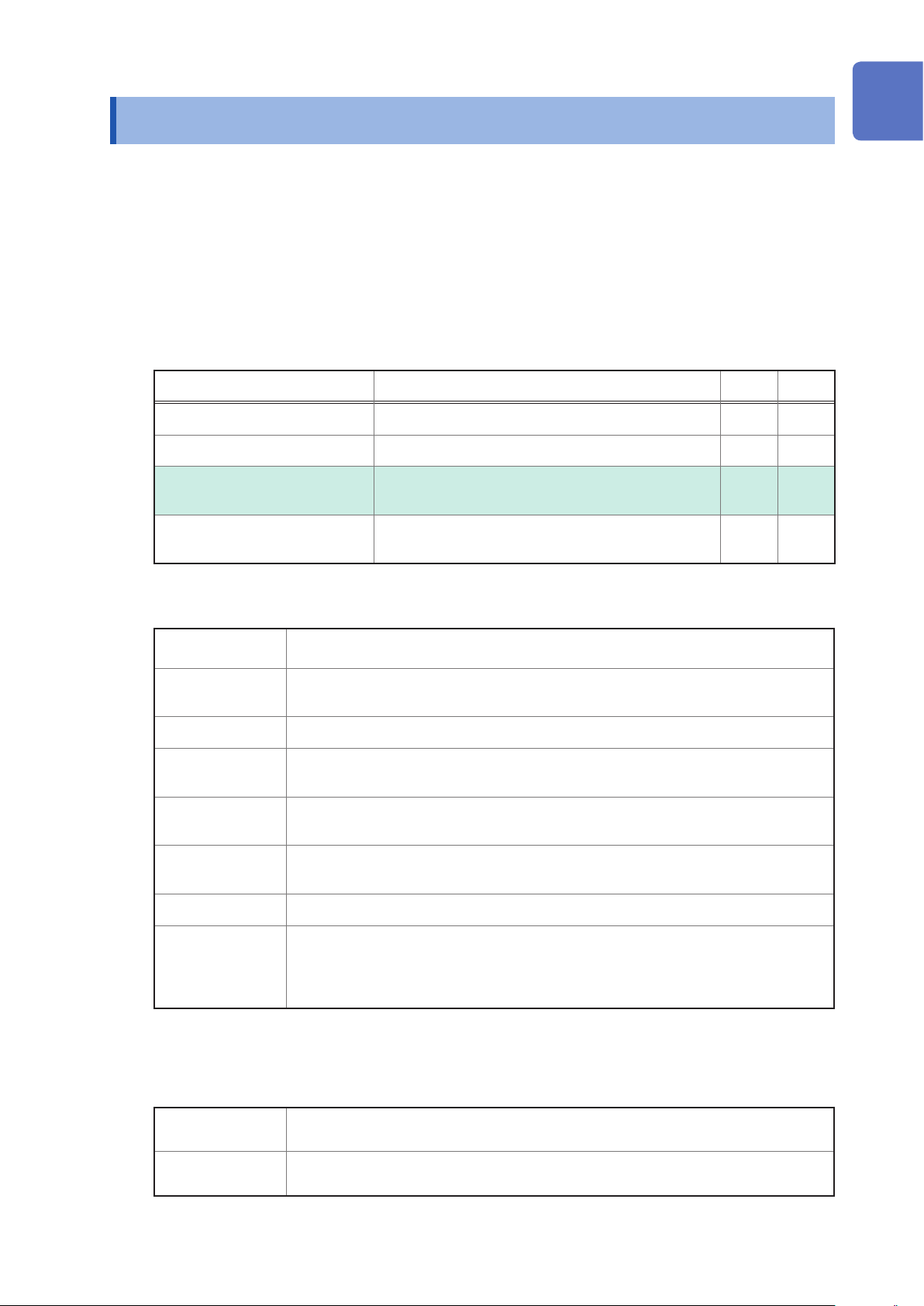
Type Contents Print PDF

Operating Precautions Information on the instrument for safe operation

Quick Start Manual Basic instructions and instrument specications

Instruction Manual (this document)

Calculation Guide (Options)

Notations

(Bold-faced)

Functions and instructions for the instrument –

Method to use the calculation functions, etc. available only with Model MR6000-01



(p. ) Indicates the location of reference information.

START

[ ]

Windows

Additional information is presented below.

Indicates the initial setting values of the items. Initialization sets the items to these values.

Indicates the names and keys on the windows in boldface.

Menus, dialogs, buttons in a dialog, and other names on the screen are indicated in brackets.

Unless otherwise specied, “Windows” represents Windows 7, Windows 8, and

Windows 10.



–



Current sensor Sensors measuring current are referred to as “current sensor.”

The number of times per second the analog input signals are digitized by the

S/s

instrument is expressed in terms of “samples per second (S/s).” Example: “20 MS/s” (20 megasamples per second) indicates that the signal is digitized

20 × 10

times per second.

Accuracy

We dene measurement tolerances in terms of f.s. (full scale), and rdg. (reading) with the following

meanings:

f.s.

rdg.

(maximum display value or scale length) The maximum displayable value or scale length.

(displayed value) The value presently being measured and indicated on the measuring instrument.

Page 6

How to Refer to This Manual

How to open a screen

Indicates the order of tapping the screens.

The button setting key.

Sequence numbers

Numbered same as a corresponding step-by-step instruction.

Options and explanations

Describes selectable settings when an item is tapped. The icon default setting of the item.

represents the



indicates the

Page 7

Measurement Method

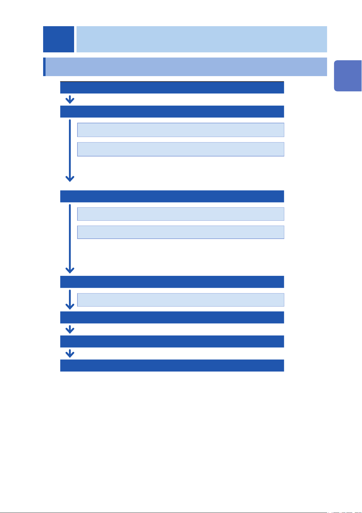
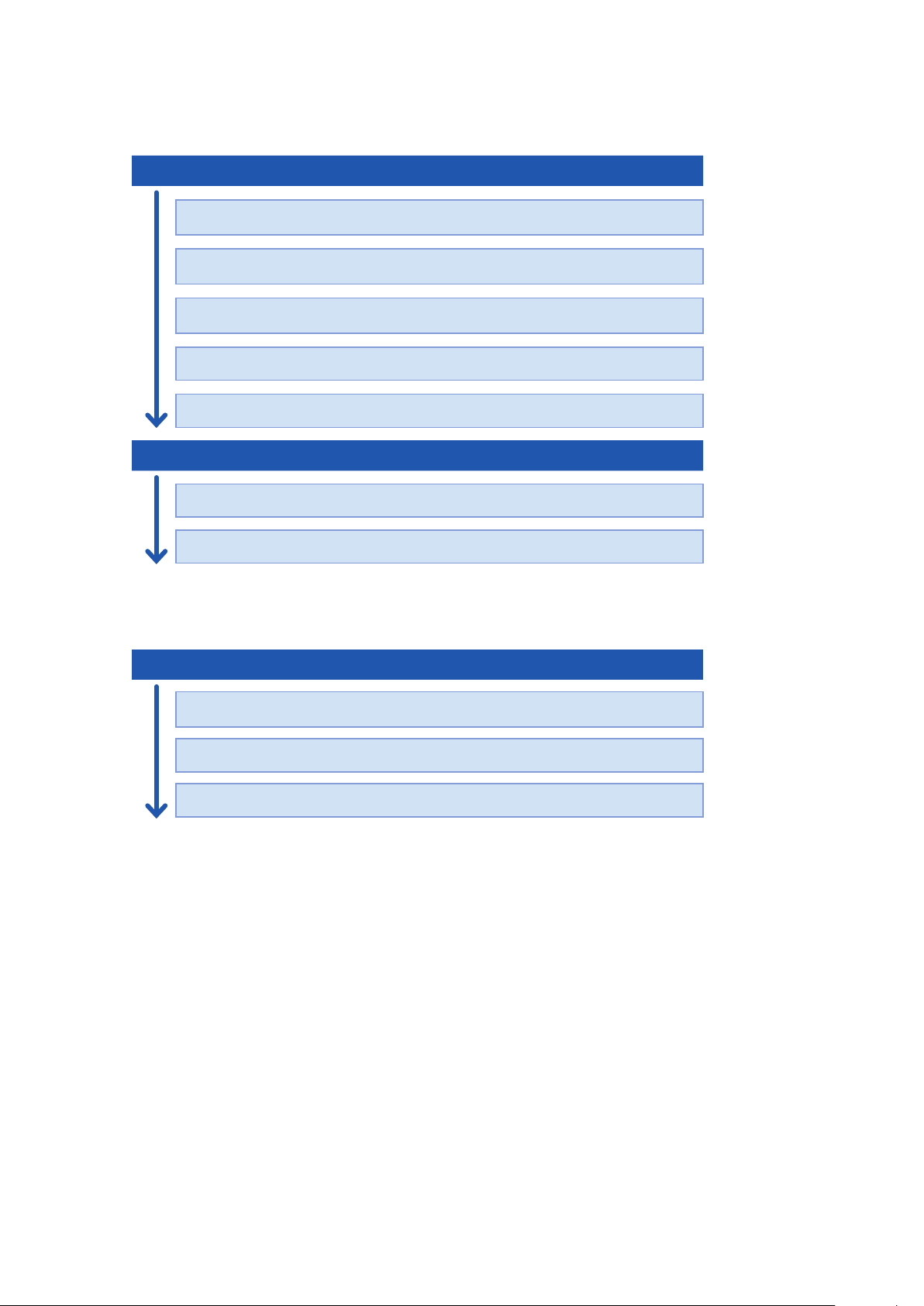
1.1 Measurement Procedure

Inspecting the instrument before measurement

Conguring the basic settings for measurement

Measurement Method

Set the sampling rate.

Set the recording length.

Advanced settings: “Using the envelope” (p. 9)

“3.1 Overlaying New Waveforms With Previously

Acquired Waveforms”

Setting the input channels

Set the analog channels.

Set the logic channels.

Advanced settings: “3.2 Converting Input Values (Scaling Function)” (p. 42)

“3.3 Fine-Adjusting Input Values (Vernier Function)” (p. 48)

“3.4 Inverting the Waveform (Invert Function)” (p. 49)

Setting the sheets

Set the display format of waveforms.

(p. 5)

(p. 6)

(p. 40)

(p. 11)

(p. 13)

(p. 17)

(p. 18)

Setting the triggers

Starting a measurement

Finishing the measurement

Advanced operation: “2.2 Specifying the Waveform Range (Section Cursor)” (p. 26)

“Scrolling waveforms” (p. 30)

“2.5 Changing the Display Position and Display

Magnication of the Waveforms”

“4 Saving/Loading Data and Managing Files” (p. 65)

“7 Numerical Calculation Function” (p. 119)

(p. 81)

(p. 20)

(p. 47)

Page 8

Measurement Procedure

To perform the automatic setup

On the waveform screen, tap [Auto range] to set the sampling rate, measurement range, and zero position of input waveforms automatically, and then start a measurement. Refer to “3.7 Measurement With the Auto-range Setting” in Quick Start Manual.

To load settings registered previously

Load the settings le on the le screen.

Refer to “4.3 Loading Data” (p. 77).

To load saved settings automatically at the time of startup

Congure the setting for the instrument so as to load the le containing the instrument settings at

the time of startup. Refer to “Loading the settings automatically (Auto-setup function)” (p. 78)

To initialize the instrument (restoring the basic settings)

Restore the instrument settings to the factory default by tapping [Initialize], which is accessible by proceeding in the following order:

> [System] > [Initialize]

The setting after the initialization is suitable for simple measurement. If any unexpected or complicated behavior is observed, initialize the instrument. Refer to “6.2 Initializing the Instrument” in Quick Start Manual.

Page 9

Conguring Measurement Conditions

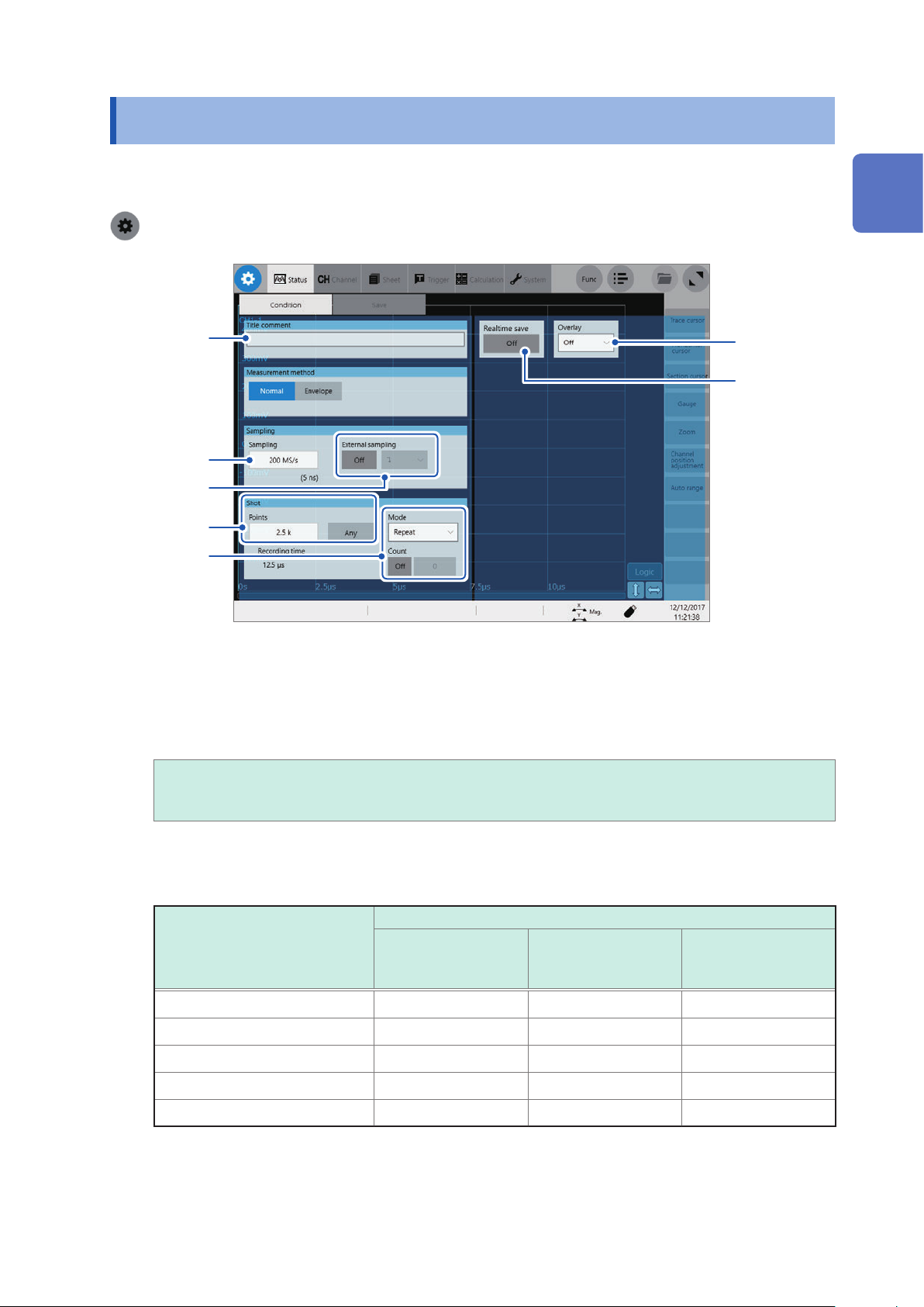
1.2 Conguring Measurement Conditions

Congure conditions required for measurement including the sampling rate ([Sampling]) and recording length ([Shot]).

> [Status] > [Condition]

Measurement Method

2 3

4 5

Type a comment in the [Title comment] box.

Number of characters: up to 40

Set [Sampling].

Refer to “Sampling rate setting guideline” (p. 7).

200 MS/s 500 kS/s, 200 kS/s, 100 kS/s, 50 kS/s, 20 kS/s, 10 kS/s, 5 kS/s, 2 kS/s, 1 kS/s, 500 S/s, 200 S/s, 100 S/s, 50 S/s, 20 S/s, 10 S/s, 5 S/s, 2 S/s, 1 S/s



, 100 MS/s, 50 MS/s, 20 MS/s, 10 MS/s, 5 MS/s, 2 MS/s, 1 MS/s,

When the real-time waveform calculation (Model MR6000-01 only) is set to [On], a sampling rate of 200 MS/s cannot be selected. When the real-time save is set to [On], due to the combination of the number of channels to be used and save destinations, the maximum sampling rate that can be set varies as follows:

Maximum sampling rate that can be set

Number of channels to be used

1 channel to 2 channels 20 MS/s 10 MS/s 5 MS/s

3 channels to 4 channels 10 MS/s 5 MS/s 2 MS/s

5 channels to 8 channels 5 MS/s 2 MS/s 1 MS/s

9 channels to 16 channels 2 MS/s 1 MS/s 500 kS/s

17 channels to 32 channels 1 MS/s 500 kS/s 200 kS/s

Only if the following Hioki-designated options are used, the real-time save operation with the instrument is guaranteed:

• Model U8332 SSD Unit

• Model U8333 HD Unit

• Model Z4006 USB Drive

• Model Z4001 and Model Z4003 SD Memory Card

SSD HDD

USB ash drive

SD card

FTP transmission

Page 10

Conguring Measurement Conditions

Set [External sampling].

The external sampling is disabled when the envelope is used.



Off

On Select this option to sample data at a sampling rate dened by a signal input into the



Set [Shot].

Tap [Points] to set the number of measurement points.



2.5 k

, 5 k, 10 k, 20 k, 50 k, 100 k, 200 k, 500 k, 1 M, 2 M, 5 M, 10 M, 20 M, 50 M, 100 M, 200 M,

500 M, 1 G

Enabling [Any] and tapping [Points] allows you to set the number of points in increments of 100. When the real-time save is set to [On], [Shot] cannot be set in terms of [Points]. Set [Recording time] on the [Save] screen. (p. 73) The maximum recording length that can be set varies depending on the number of channels to be measured.

Disables the external sampling function.

external sampling terminal (EXT.SMPL).

Samples data at rising edges of the input signal.

Samples data at falling edges of the input signal.

Set [Mode].

Single Measures waveforms only once. Pressing the START key starts recording waveforms,

and then stops when the specied recording length of the waveforms have been acquired.

Repeat

When [Repeat] mode is set and [Count] is set to [On], the specied number of measurements are performed. Only [Single] mode can be selected when [Realtime save] is set to [On].

Set [Overlay].

Refer to “3.1 Overlaying New Waveforms With Previously Acquired Waveforms” (p. 40).

Set [Realtime save] to [On].

Data can be recorded in the optional storage device while measuring waveforms. Refer to “Real-time save” (p. 72).



Measures waveforms repeatedly. Pressing the STOP key stops the measurement in progress.

Page 11

Sampling rate setting guideline

Select a sampling rate using the following table as a guideline.

Conguring Measurement Conditions

Maximum display

frequency

8 MHz 200 MS/s 400 Hz 10 kS/s

4 MHz 100 MS/s 200 Hz 5 kS/s

2 MHz 50 MS/s 80 Hz 2 kS/s

800 kHz 20 MS/s 40 Hz 1 kS/s

400 kHz 10 MS/s 20 Hz 500 S/s

200 kHz 5 MS/s 8 Hz 200 S/s

80 kHz 2 MS/s 4 Hz 100 S/s

40 kHz 1 MS/s 2 Hz 50 S/s

20 kHz 500 kS/s 0.8 Hz 20 S/s

8 kHz 200 kS/s 0.4 Hz 10 S/s

4 kHz 100 kS/s 0.2 Hz 5 S/s

2 kHz 50 kS/s 0.08 Hz 2 S/s

800 Hz 20 kS/s 0.04 Hz 1 S/s

Sampling rate

Maximum display

frequency

Sampling rate

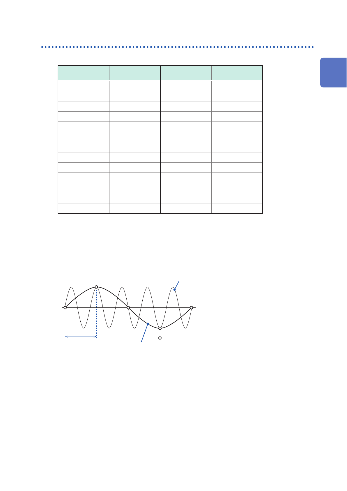
If the instrument plots non-existent waveforms (aliasing)

If a measured signal oscillates at a higher frequency compared to the specied sampling rate, the instrument may plot non-existent waveforms oscillating at a lower frequency than that of the actual signal when the signal frequency reaches a certain level. This phenomenon is called aliasing.

Measurement Method

Actual input signal

A sampling interval longer than the cycle of the input signal causes aliasing.

Sampling interval

To plot a sign wave that allows you to observe the peaks of the sine wave on the LCD without any aliasing, the instrument needs to sample the waveform at a minimum of 25 points per cycle.

Observed waveform

: Sampled points

To set the sampling rate automatically

Refer to “3.7 Measurement With the Auto-range setting” in Quick Start Manual.

Page 12

Conguring Measurement Conditions

Update rate of each module

The data update rate is not allowed to exceed the maximum sampling rate of each module. The same data are measured until they get updated, causing the instrument to plot a stair-step waveform. In addition, even though the same signal is measured simultaneously, values may vary due to

differences in the sampling rate, frequency range, and frequency characteristics of modules.

Module Sampling rate of module Reference

Model 8966 Analog Unit 20 MS/s (50 ns) –

Model 8967 Temp Unit

Model 8968 High Resolution Unit 1 MS/s (1 µs) –

Model U8969 Strain Unit 200 kS/s (5 µs) p. 54

Model 8970 Freq Unit Varies according to the setting. p. 56

Model 8971 Current Unit 1 MS/s (1 µs) p. 59

Model 8972 DC/RMS Unit Varies according to the response setting. p. 61

Model 8973 Logic Unit 20 MS/s (50 ns) –

MR8990 Digital Voltmeter Unit

Model U8974 High Voltage Unit 1 MS/s (1 µs) p. 64

Model U8975 4ch Analog Unit 5 MS/s (200 ns) –

Model U8976 High Speed Analog Unit 200 MS/s (5 ns) –

Varies according to the data refresh setting.

Varies according to the NPLC setting. p. 62

p. 52

Page 13

Using the envelope

> [Status] > [Condition]

Conguring Measurement Conditions

Measurement Method

Set [Measurement method] to [Envelope].

Normal

Envelope Uses the envelope.

• Normal:

• Envelope:

• Values to be acquired using the envelope

A set of sampled data acquired using the envelope consists of two values: the maximum value and the minimum value. These values are taken from the measured values acquired at an over-sampling rate during

the recording interval set in [Sampling]. When shown on the screen, they are displayed as if they range in amplitude. When saved in an external storage device, the data of the maximum and minimum values are stored for a single instance of measurement.



The instrument records data at the specied sampling rate.

At the specied recording interval, the instrument records the maximum and minimum values among data sampled within each specied recording interval at an over-sampling rate* of 100 MS/s. Hence, even though a relatively longer recording interval is set, peaks of uctuations can be recorded without being missed.

*: Over-sampled data (indicated by blue dots

Recording

interval

Oversampling interval (10 ns)

Does not use the envelope.

Maximum

Minimum

in the gure) are not saved.

: Over-sampled data : Stored data (data of the maximum and minimum

values)

: Waveform shown on the screen

Page 14

Conguring Measurement Conditions

Set [Sampling].

The following are the sampling rates that can be selected when the envelope is used.

10 MS/s 5 kS/s, 2 kS/s, 1 kS/s, 500 S/s, 200 S/s, 100 S/s, 50 S/s, 20 S/s, 10 S/s, 5 S/s, 2 S/s, 1 S/s, 30 S/min, 12 S/min, 6 S/min, 2 S/min, 1 S/min

Set [Shot].

Tap [Points] to set the number of measurement points.

2.5 k 500 M, 1 G

Enabling [Any] and tapping [Points] allows you to enter [Points] in increments of 100 points. When the real-time save is set to [On], [Shot] cannot be set in terms of [Points]. Set [Recording time] on the [Save] screen. (p. 73) The maximum recording length that can be set varies depending on the number of channels to be measured.



, 5 MS/s, 2 MS/s, 1 MS/s, 500 kS/s, 200 kS/s, 100 kS/s, 50 kS/s, 20 kS/s, 10 kS/s,



, 5 k, 10 k, 20 k, 50 k, 100 k, 200 k, 500 k, 1 M, 2 M, 5 M, 10 M, 20 M, 50 M, 100 M, 200 M,

Page 15

1.3 Setting Input Channels

Congure the settings of the analog and logic channels.

Setting Input Channels

> [Channel]

Operation available on the [Channel] screen

• Adding a comment to a channel

• Setting measurement conditions for a channel

• Setting the display method of waveforms

• Converting measured values into physical quantities and displaying them

Measurement Method

Page 16

Setting Input Channels

Channel setting procedure

Analog channels (CH1 through CH32) setting procedure

Conguring input settings

Set the measurement mode.

Select an appropriate range for measurement.

Convert input values. (Scaling function)

Set the input coupling.

Set the low-pass lter (if noise is observed).

Conguring the display settings

Set the display color of waveforms.

Convert input values. (Scaling function)

Logic channels (Model 8973 Logic Unit) setting procedure

(p. 13)

(p. 14)

(p. 16)

(p. 15)

(p. 16)

Conguring the display settings

Set the logic recording width.

Set the display positions of waveforms.

Set the display colors of waveforms.

(p. 17)

Page 17

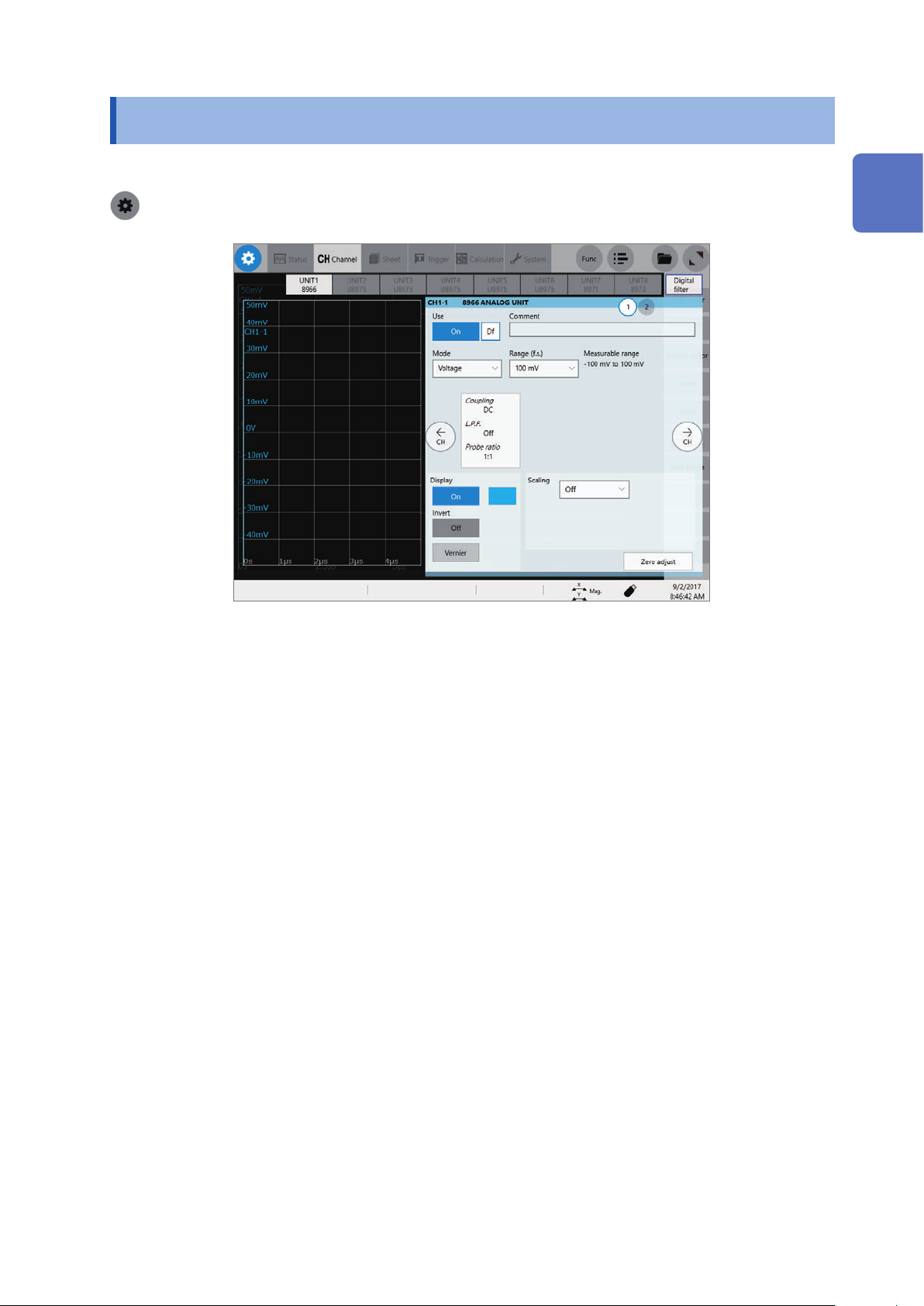
Setting Input Channels

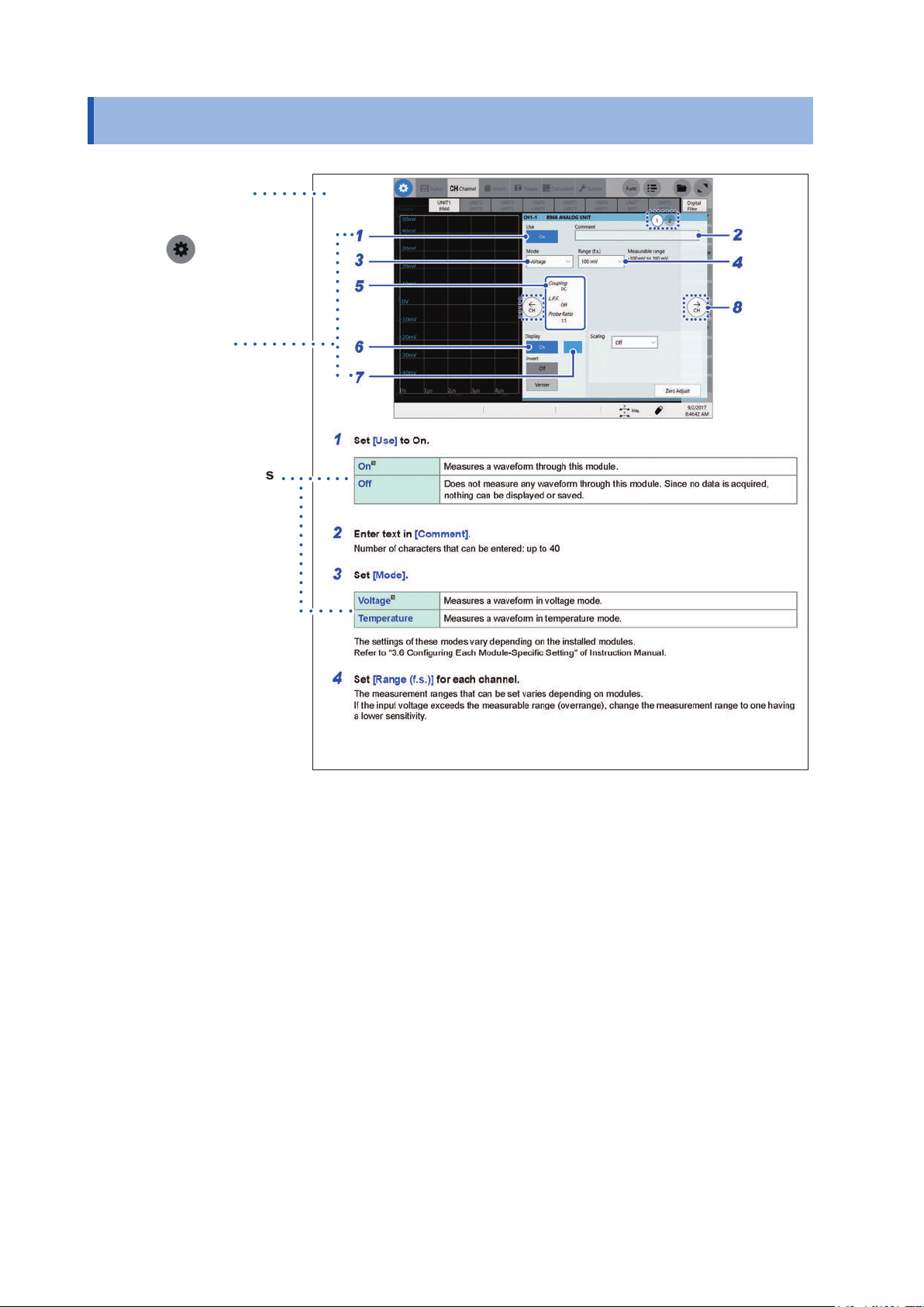
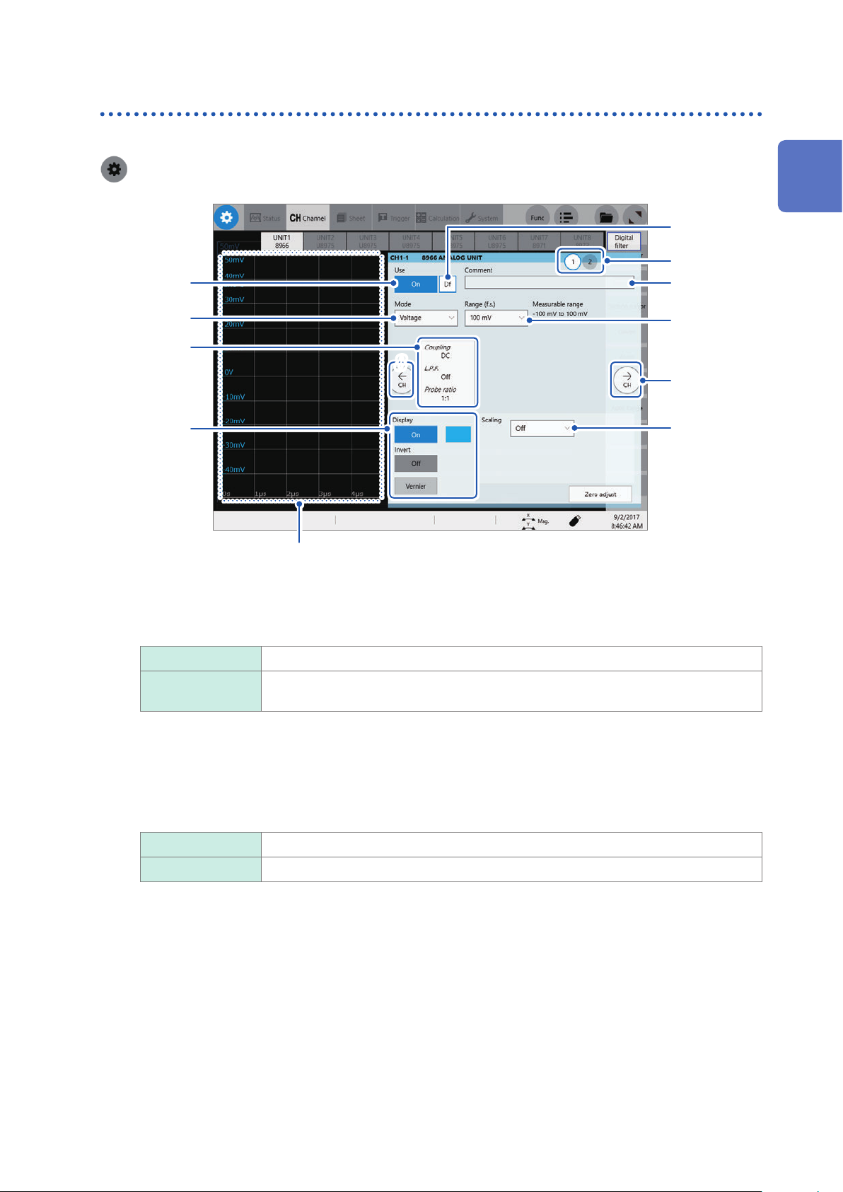
Analog channels

For details on setting each module, refer to “3.6 Conguring Module-Specic Settings” (p. 51).

> [Channel] > [UNIT]

Measurement Method

9 8

3 5

The waveform screen is displayed during measurement. When no measurement is not performed, the presently input waveforms are displayed on the monitor.

Set [Use] to [On] or [Off].



Off Does not set the module as the measurement device.

Sets the module as the measurement device.

Since no data is acquired, nothing can be displayed or saved.

Type a comment in the [Comment] box.

Number of characters: up to 40

Set [Mode].

Voltage

Temperature Measures a waveform in temperature mode.

Settings vary depending on the installed modules.

Refer to “3.6 Conguring Module-Specic Settings” (p. 51).



Measures a waveform in voltage mode.

Page 18

Setting Input Channels

Set [Range (f.s.)].

Set the measurement range for each channel. The value of the range represents its maximum displayable value (f.s.). See the following table for the full-scale resolution of each module. If the input voltage exceeds the measurable range (overrange occurs), change the measurement range to one having a lower sensitivity. After changing [Range (f.s.)], check the [Level], [Upper], [Lower], and other values of the trigger, search, and numerical calculation functions.

Module Resolution [LSB]

Model 8966 Analog Unit, Model 8971 Current Unit, Model 8972 DC/RMS Unit 2,000

Model 8967 Temp Unit 20,000

Model 8968 High Resolution Unit, Model U8974 High Voltage Unit, Model U8975 4ch Analog Unit

Model U8976 High Speed Analog Unit 1,600

Model U8969 Strain Unit 25,000

Model 8970 Freq Unit (Power frequency mode) 2,000

Model 8970 Freq Unit (Count mode) 40,000

Model 8970 Freq Unit (Frequency mode, rotation speed mode, duty ratio mode, pulse width mode)

Model MR8990 Digital Voltmeter Unit 1,000,000

*: For the Model 8967 Temp Unit, the valid range varies depending on the thermocouples. For more

information about resolution, refer to “Model 8967 Temp Unit” in “5.2 Specications for Options” in Quick

Start Manual.

32,000

10,000

Page 19

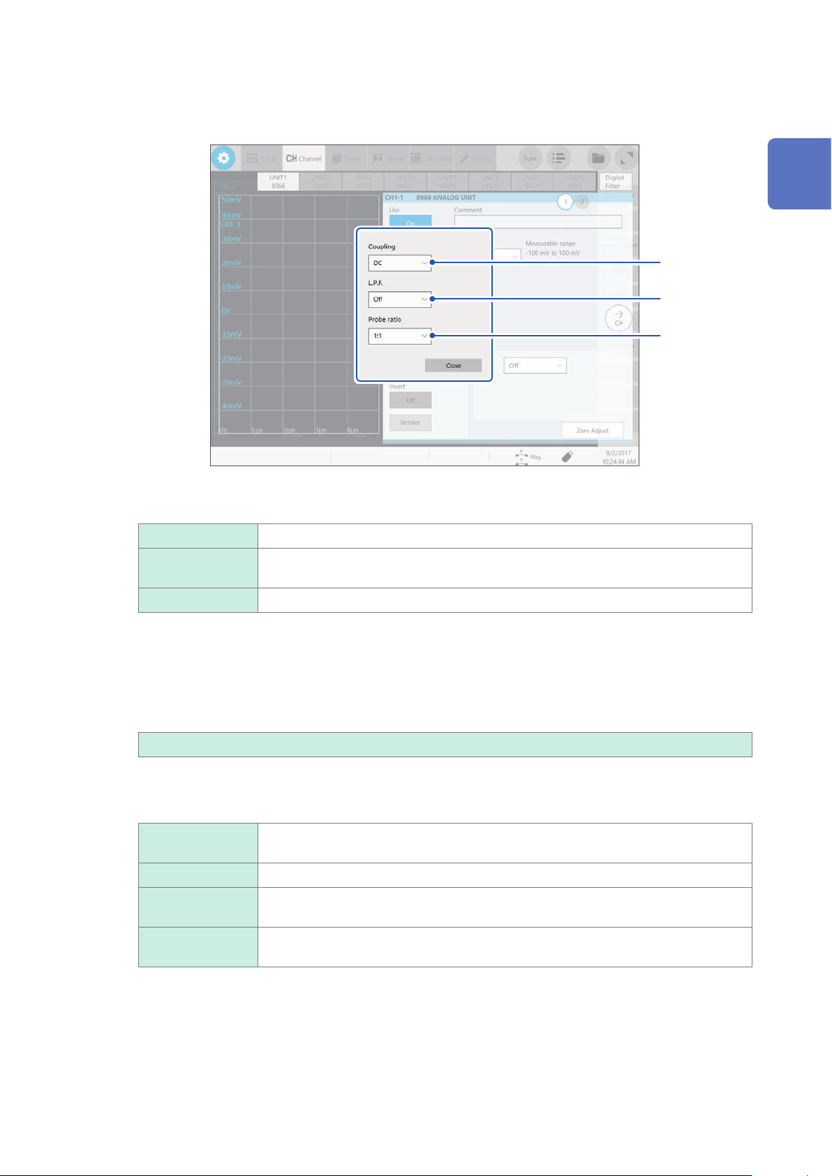
Set [Coupling], [L.P.F.], and [Probe ratio].

Tap the screen to open the settings dialog box.

Setting Input Channels

Measurement Method

(1)

(2)

(3)

(1) Set [Coupling].

The input signal coupling method can be specied. In general, use the DC coupling.



AC Measures an AC component only of an input signal. A DC component can be

GND Connect the input terminal to the ground (Enables you to check the zero position).

Measures both DC and AC components of an input signal.

eliminated.

(2) Set [L.P.F.] (low-pass lter).

Enabling the low-pass lter installed in the module allows elimination of unwanted high-frequency components. The lters that can be set varies depending on the type of modules. Select a lter according to the

characteristics of the input signals. Example: For Model 8966 Analog Unit



Off

, 5 Hz, 50 Hz, 500 Hz, 5 kHz, 50 kHz, 500 kHz

(3) Set [Probe ratio].

Select this setting when the measurement is to be performed with a connection cable or probe.



1:1

1:10 Select this option when using Model 9665 10:1 Probe.

Select this option when using Model L9197, Model L9198, Model L9790, or Model L9217 Connection Cord.

1:100 Select this option when using Model 9666 100:1 Probe, Model P9000-01 Differential

Probe, or Model P9000-02 Differential Probe.

1:1000 Select this option when using Model 9322 Differential Probe, Model P9000-01

Differential Probe, or Model P9000-02 Differential Probe.

Page 20

Setting Input Channels

Set [Display].



Displays the waveforms on the waveform screen.

Color Allows you to select display colors of the waveforms. You can also select the

same color as the lines acquired through other channels.

Invert



, On)

(Off

Vernier Allows you to ne-adjust the input voltage freely on the waveform screen

Off Displays no waveforms.

Set [Scaling].

Refer to “3.2 Converting Input Values (Scaling Function)” (p. 42).

Switch the channels.

Tap the corresponding location to switch the channels.

Set [Digital lter] for each channel. (Model MR6000-01 only)

The [Df] setting is displayed for only channels with [Digital lter] set to [On], allowing you to set the digital

lter for each channel.

For more information, refer to “Setting the Digital Filter Calculation” in Calculation Guide.

When the signs of displayed waveforms are reversed, the waveforms can be inverted. Refer to “3.4 Inverting the Waveform (Invert Function)” (p. 49).

(display adjustment only). When recording physical values such as noise, temperature, and acceleration with sensors, you can adjust those amplitudes,

facilitating calibration.

Refer to “3.3 Fine-Adjusting Input Values (Vernier Function)” (p. 48).

Page 21

Setting Input Channels

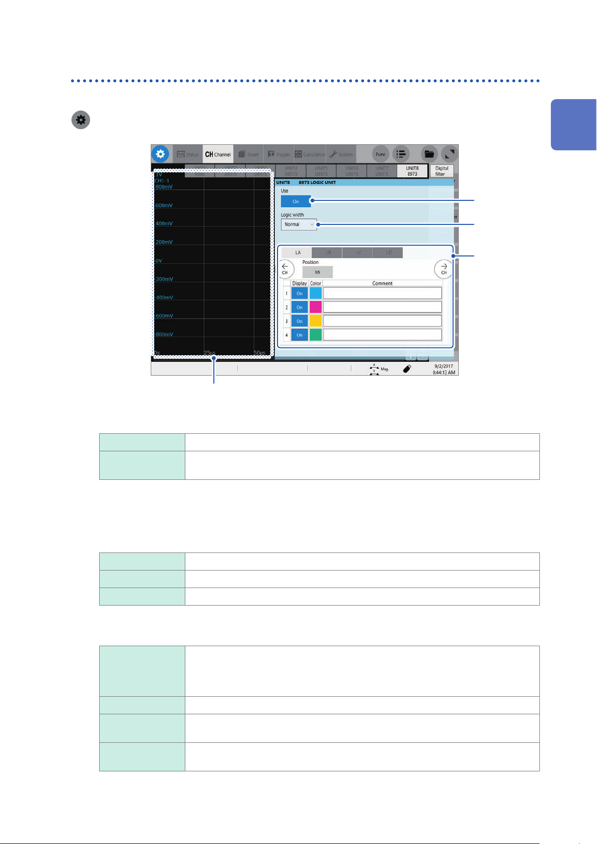
Logic channels

The logic sheet is displayed when the screen is in Single, Dual, Quad, Octa, or Hexadeca mode.

> [Channel]

Measurement Method

The waveform screen is displayed when a logic channel is selected. Positions of the logic display can be checked.

Set [Use] to [On] or [Off].



Off Does not set the module as the measurement device.

Set [Logic width].

You can change the display width of the logic waveforms. Making waveforms narrower can enhance the readability of a display that contains a large number of waveforms. This setting is shared by all installed logic modules.

Wide Increases the width of the waveforms.

Normal

Narrow Reduces the width of the waveforms.

Select a display method for each probe (LA through LD).

Position Allows you to set the position of the logic waveforms within the display range. The



Sets the module as the measurement device.

Since no data is acquired, nothing can be displayed or saved.

Displays the waveforms in normal width.

position of the waveforms can be set in increments of one percent point. This setting is shared by all probes (LA through LD). You can move the logic position freely within the screen limits.

Display Sets whether to display each logic waveform.

Color Allows you to select a display waveform of each waveform. You can also select the

same color as the lines acquired through other channels.

Comment Allows you to type a comment for each channel.

Number of characters: up to 40

Page 22

Setting the Sheets

1.4 Setting the Sheets

You can dene the display format of waveforms on the sheet. You can dene different display

formats for each of the 16 sheets. You can also switch the sheets to be displayed on the waveform screen.

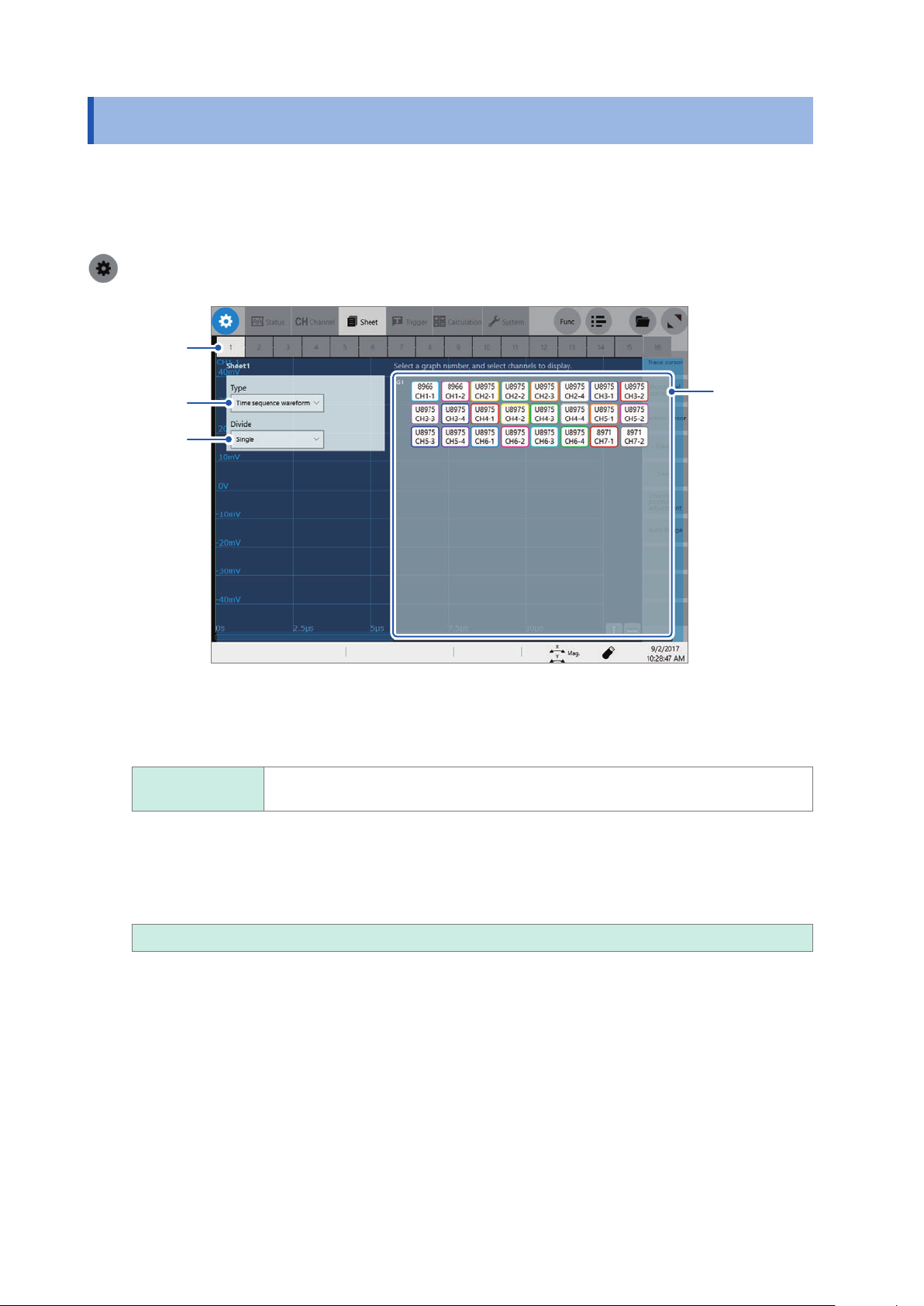
> [Sheet]

Select a sheet.

Set [Type].

Time sequence waveform

2 3



Displays time-sequence waveforms.

Set [Divide].

You can divide the screen into multiple screens (graphs). The options when [Type] is set to [Time sequence waveform] are as follows:



Single

Assign channels to the graph.

Tap the display panel of each graph to open the [Select the channel] dialog box.

, Dual, Quad, Octa, Hexadeca

Page 23

Setting the Sheets

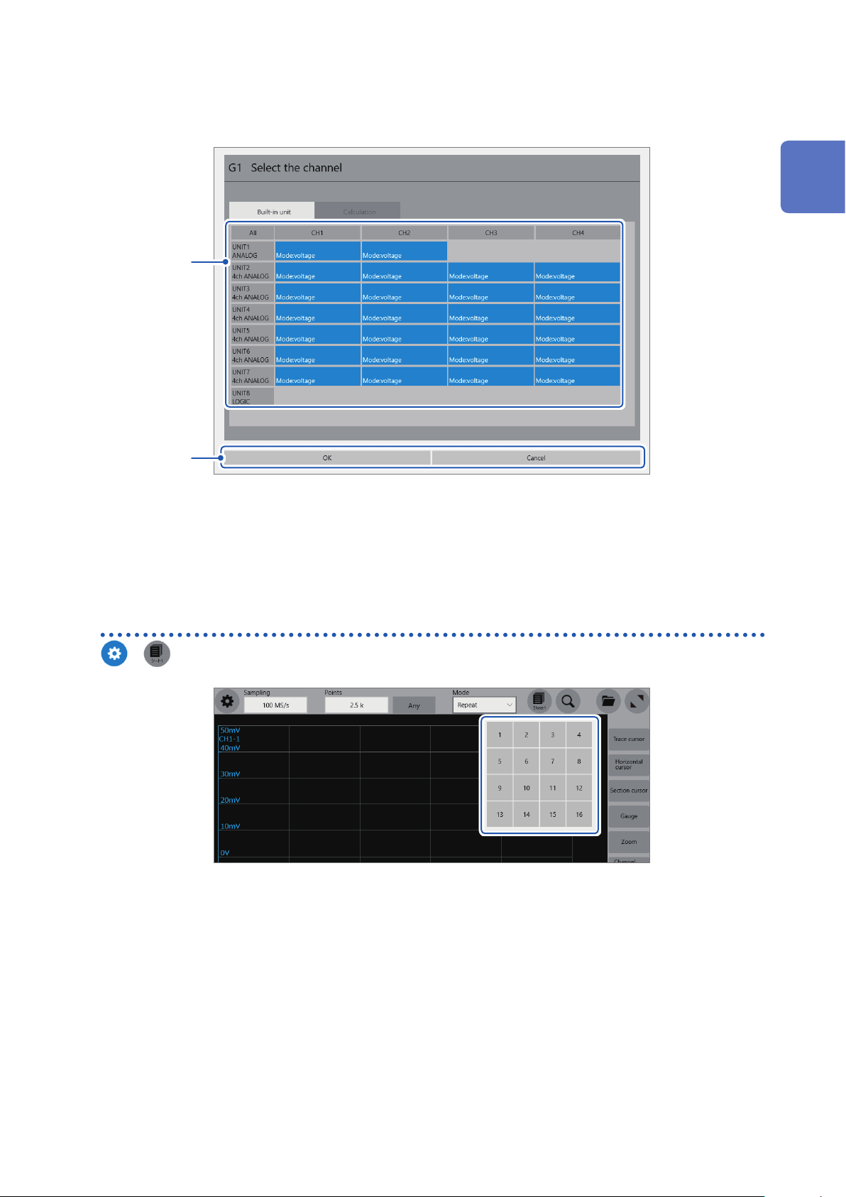
Select the channels to be displayed on the graph.

All channels are selected in the default setting. Tap a button to deselect a channel (Tap it again to select it).

Measurement Method

Tap [OK].

The selection is conrmed.

Tapping [Cancel] closes the dialog box without your selection conrmed.

Switching sheets on the waveform screen

Select the sheet numbers to be displayed.

Page 24

Starting/Stopping the Measurement

1.5 Starting/Stopping the Measurement

Starting a measurement

Pressing the START key starts a measurement.

• Waveform data displayed on the screen is cleared once the measurement starts.

• You can also start the measurement by inputting signal into the external control terminal.

Refer to “10 Controlling the Instrument Externally” (p. 179).

Waveform display during measurement

In general, the waveforms are displayed after the specied recording length of data has been acquired. When the measurement is performed at a relatively slow speed, the waveforms are displayed while the data is being acquired.

However, even if a slow-speed range is set, the waveforms are displayed after the data of the

whole waveform has been acquired, depending on the overlay or magnication setting.

To save data automatically during measurement

Refer to “Saving waveform data automatically” (p. 68).

Stopping the measurement

Pressing the STOP key once stops the measurement after the waveforms of the specied recording

length have been acquired.

Pressing the STOP key twice stops the measurement immediately.

Page 25

Operating the Waveform Screen

and Analyzing Data

You can analyze measured data with various functions including trace cursor measurement and search of input waveforms on the waveform screen. You can also change measurement conditions

or other conguration on this screen.

Operating the Waveform Screen and Analyzing Data

Operation available on the waveform screen

Use the trace cursors

• Reading measured values (p. 22)

Moving the waveform display position

• Moving waveforms by dragging them

• Moving waveforms with the scroll bar

Use the section cursors

• Specifying the waveform range (p. 26)

Changing the display magnication of

waveforms

• Magnifying/demagnifying waveforms (p. 32)

• Magnifying a part of waveforms horizontally (p. 37)

Page 26

Reading Measured Values (Trace Cursors)

2.1

Reading Measured Values (Trace Cursors)

Using trace cursors on the waveform screen allows you to read measured values (scaled value when the scaling is used). Up to eight trace cursors can be displayed simultaneously. You can read differences in times and measured values at any two selected among them. The time lag, for example, shows the difference in time between Trace cursor A and Trace cursor B when they are enabled.

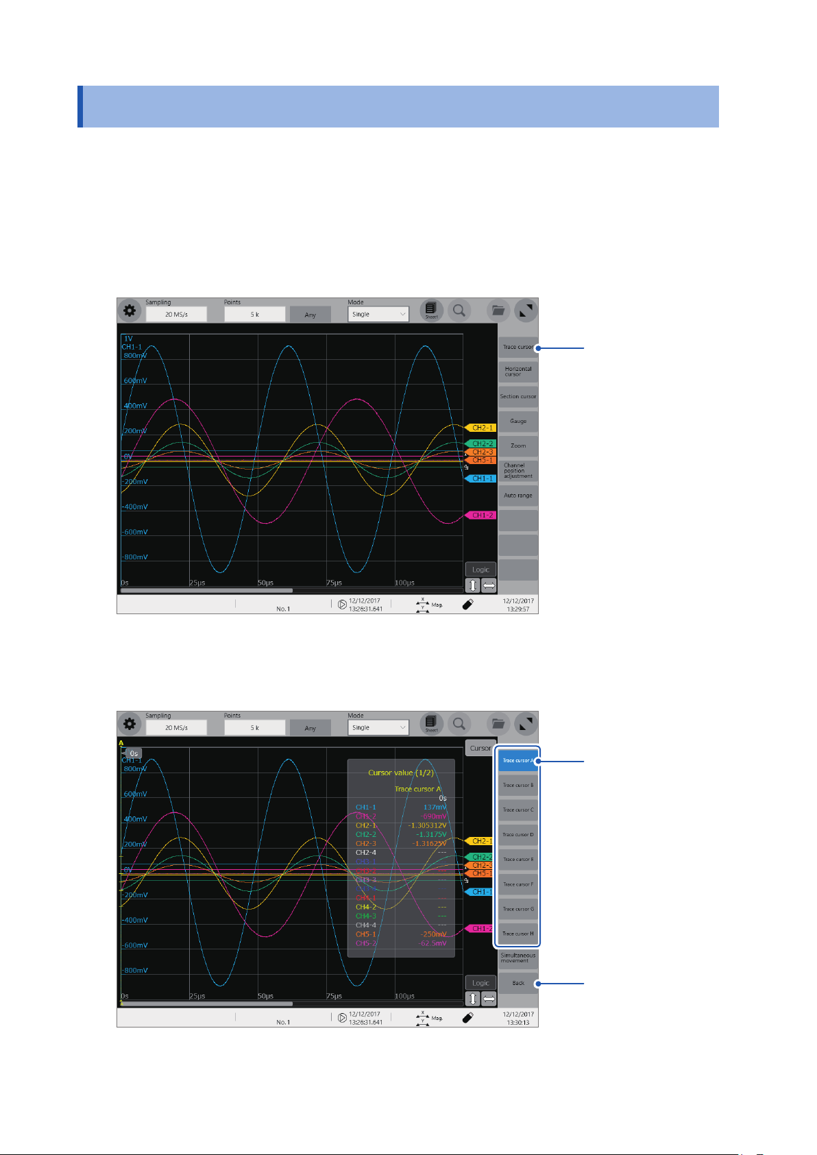
Tap [Trace cursor].

Select one or more cursors from [Trace cursor A] through [Trace cursor H] by tapping them.

The selected trace cursors are displayed on the waveform screen. Move the trace cursors by dragging them on the waveform screen.

Tap [Back].

Page 27

Reading Measured Values (Trace Cursors)

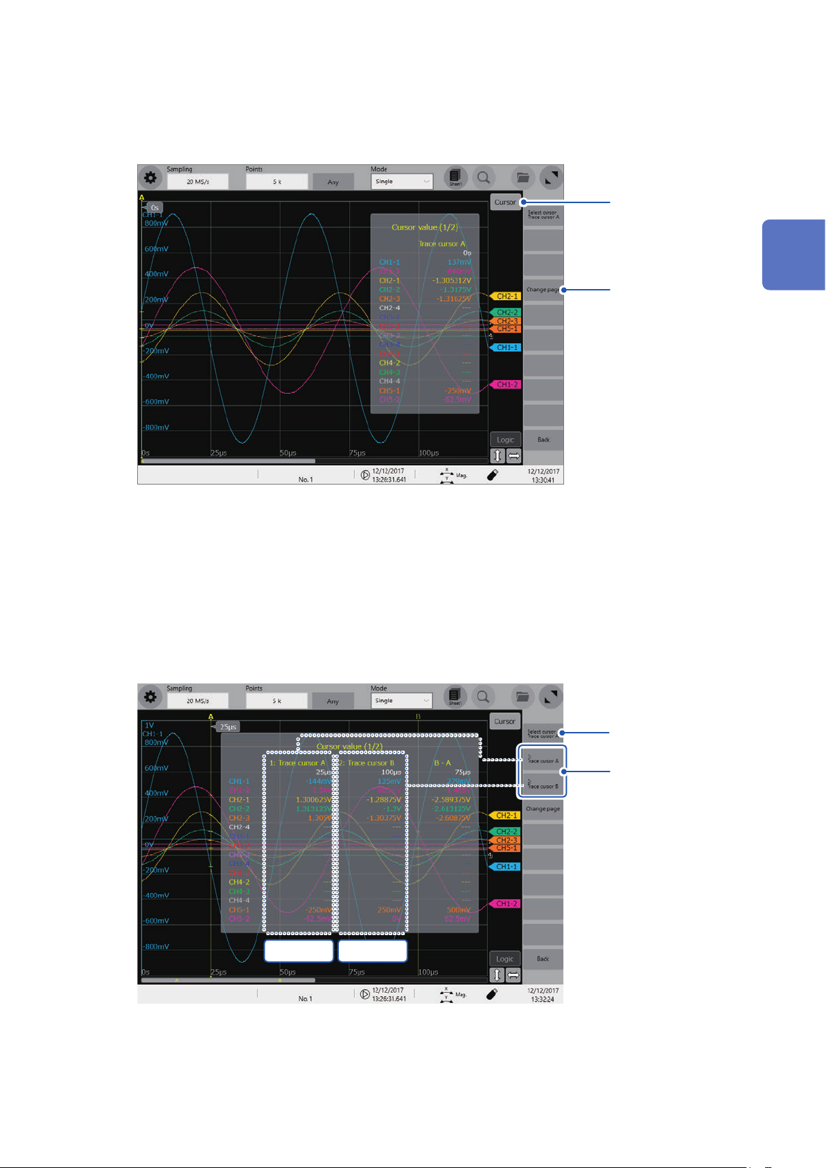
Tap [Cursor].

The cursor value display can be switched between on and off every time tapped.

[Cursor]

Tap [Change page].

If multiple channels are displayed, switch the pages to check the cursor values of each channel. Every time it is tapped, the pages are switched.

Tap [1: Trace cursor] or [2: Trace cursor].

When the multiple trace cursors are displayed, the cursor values acquired at the two trace cursors are displayed on the waveform screen (Cursor values 1 and 2). Every time you tap [1: Trace cursor] (or [2: Trace cursor]), the values of Cursor values 1 (or Cursor values 2) switches from one to another.

Operating the Waveform Screen and Analyzing Data

Cursor values 1 Cursor values 2

Page 28

Reading Measured Values (Trace Cursors)

Tap [Select cursor].

Every time you tap by one in sequence. In addition, you can activate any one of the cursors displayed on the screen by tapping it.

[Select cursor]

when the multiple trace cursors are displayed, a cursor is activated one

Changing the magnication of the waveform display while moving the trace

cursor

Sliding your nger upward on the screen while dragging the trace cursor enlarges the waveform display centered around the trace cursor in proportion to the dragging distance. Sliding your nger

downward compresses the waveform display. Once you have adjusted the display to a suitable size, move the trace cursor along the horizontal axis to change the display position.

Releasing your nger from the screen reverts the display to the original magnication.

To move the trace cursor using the rotary knob X

When [Cursor] is assigned to the rotary knob, you can move the active trace cursor with the rotary knob X.

If the trace cursor is not displayed on the screen even though it is enabled

Check the position of the trace cursor on the scroll bar. (p. 31)

Page 29

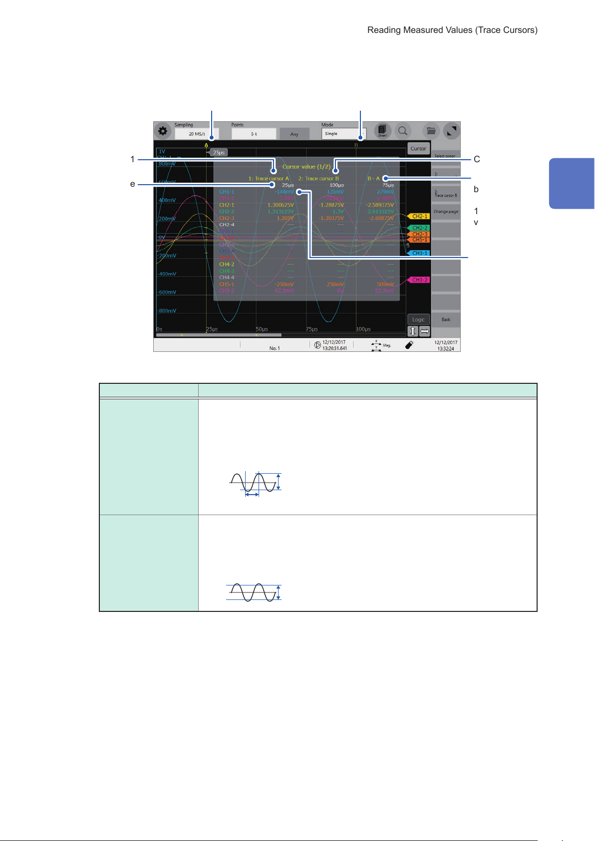
Reading measured values on the waveform screen

A B

When the trace cursor is selected

Reading Measured Values (Trace Cursors)

Trace cursor A

Cursor value 1 Cursor value 2

Time

Trace cursor B

Difference between Cursor value 1 and Cursor value 2

The values of the points at which each cursor crosses the waveforms are displayed.

The display of the cursor values vary depending on the selected cursor type.

Cursor type Cursor value

Trace cursor

When Trace cursor A is assigned to Cursor value 1; and Trace cursor B, to Cursor value 2. Time: A period of time from the trigger point or starting point of recording until the

trace cursor selected for Cursor value 1 or Cursor value 2

B − A: Difference in measured values between Trace cursor A and Trace cursor B

Operating the Waveform Screen and Analyzing Data

B − A (Difference between measured values)

B − A (Time lag)

Horizontal cursor

When Horizontal cursor A is assigned to Cursor value 1; and Horizontal cursor B, to Cursor value 2

Cursor value 1 or Cursor value 2: Measured value of the specied cursor B − A: Difference in measured values between Horizontal cursor A and Horizontal

cursor B

B − A

When the external sampling is used, the time is replaced with the number of samples.

Page 30

Specifying the Waveform Range (Section Cursor)

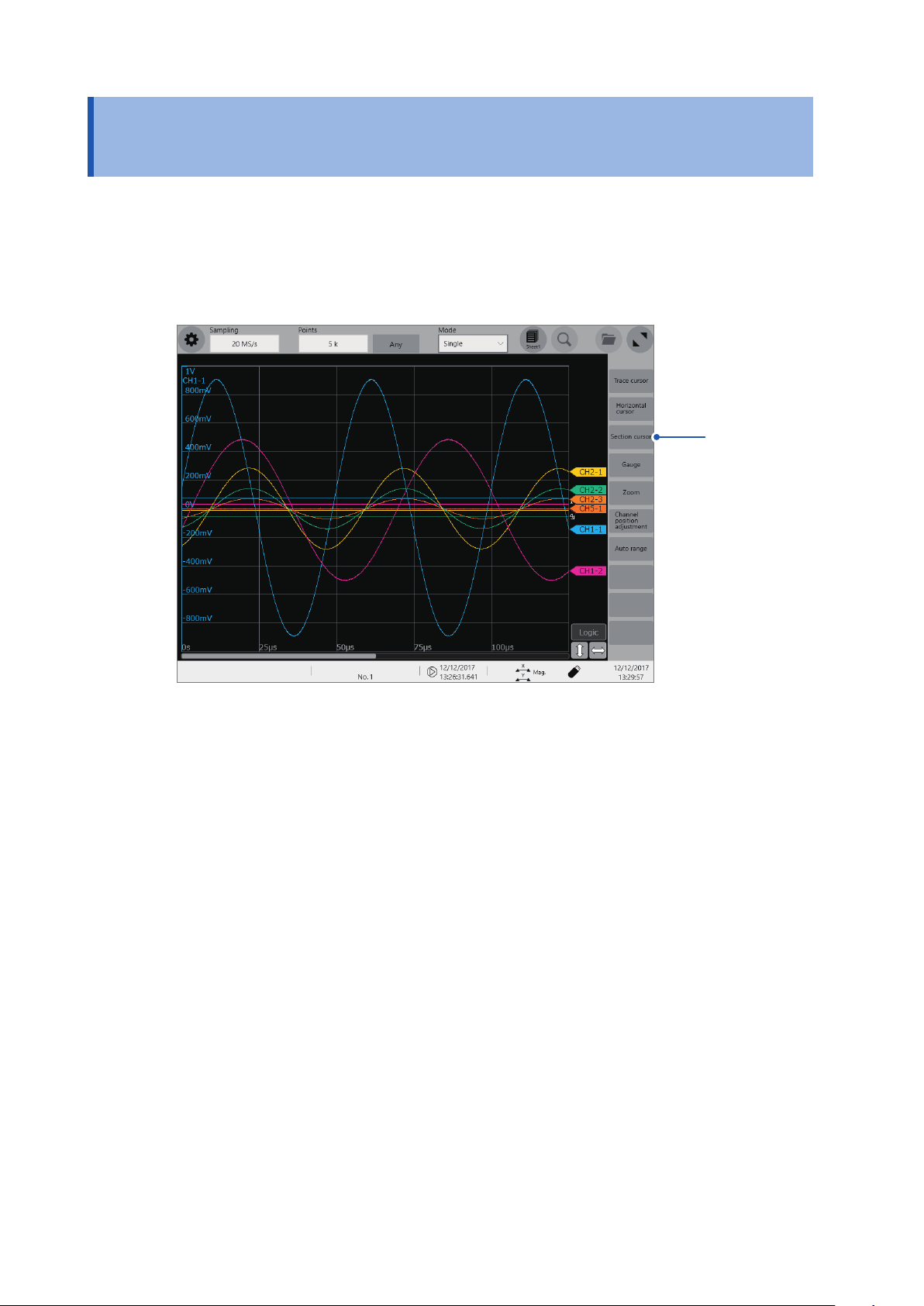
2.2 Specifying the Waveform Range (Section Cursor)

The range can be specied with section cursors. The specied range is applicable for le saving, the numerical calculation, and search. The range

selection remains to be common even when the waveform display format is changed.

Tap [Section cursor].

Page 31

Specifying the Waveform Range (Section Cursor)

Tap [Section cursor 1] or [Section cursor 2].

The cursor is displayed on the left side of the screen. You can move the section cursors or each cursor on the waveform screen by dragging one of them.

Section cursor 1 Species the section with Cursor 1A and Cursor 1B.

Section cursor 2 Species the section with Cursor 2A and Cursor 2B.

Cursor 1A Cursor 2B

Operating the Waveform Screen and Analyzing Data

Changing the display magnication of the waveforms while moving

the section cursor

Sliding your nger upward on the screen while dragging the section cursor enlarges the waveform

display centered around the section cursor in proportion to the dragging distance (Sliding your

nger downward compresses the waveform display.).

Once you have adjusted the display to a suitable size, move the section cursor along the horizontal axis to change the display position.

Releasing your nger from the screen reverts the display to the original magnication.

Page 32

Displaying Vertical Scales (Gauge Function)

2.3 Displaying Vertical Scales (Gauge Function)

Using the gauge function enable the vertical scales (for convenience, hereafter referred to as “gauges”) to be displayed overlapping waveforms.

Tap [Gauge].

Select gauges to be displayed from [Gauge A] through [Gauge H].

Gauges are displayed at the left of the screen. To move a gauge, tap the gauge, thereby it is selected, and drag it.

Tapping [Left-justied] aligns the gauges to the left.

Page 33

Tap [CH ] or [CH ].

You can switch channels to be displayed along with the guage.

Displaying Vertical Scales (Gauge Function)

Operating the Waveform Screen and Analyzing Data

Tapping [Hide] hides the gauges.

Tap [Upper and lower limit value].

The setting dialog box is displayed, which allow you to set the channel display range numerically. Type the upper and lower values in the [Upper] and [Lower] boxes, respectively, and then tap [OK].

Page 34

Scrolling Waveforms

2.4 Scrolling Waveforms

Scrolling waveforms

Dragging the waveform screen scroll the waveforms that are being measured or existing waveforms.

Scrolling direction

Screen display

Previous Latest

Dragging the waveform rightward: Scrolls the waveform backward from the present.

To anchor the waveforms vertically

Tap the button to deselect it as the scroll direction.

To anchor the waveforms horizontally

Dragging the waveform leftward: Scrolls the waveform forward from the present.

Tap the button to deselect it as the scroll direction.

To observe waveforms obtained previously during slow-speed measurement

When the waveform is being displayed during a slow-speed measurement, dragging the waveform screen allows you to observe waveforms obtained previously. To observe the waveform being measured presently again, tap [

] on the screen.



Page 35

Scrolling Waveforms

Checking a position of waveforms with the scroll bar

The scroll bar provides the position and size of the displayed part of the waveforms relative to the entire recording length of the waveforms. It also shows the positions of the trigger point, trace cursors, and section cursors.

Operating the Waveform Screen and Analyzing Data

Scroll bar

Verifying the position of the trigger point and cursors on the scroll bar

Trigger point

Section cursor position

Screen display range

With the display zoomed in, the scroll bars are displayed at both the top and bottom.

Trace cursor A

Recorded range

Page 36

Changing the Display Position and Display Magnication of the Waveforms

2.5 Changing the Display Position and Display Magnication of the Waveforms

Pinch in or out waveforms on the waveform screen to change the display magnication.

Pinch out

Pinch in

Magnies the waveforms.

Demagnies the waveforms.

To change the display position of logic channels in a batch

Select [Logic] and drag waveforms on the waveform screen to move logic channels only. When [Logic] is not selected, only analog channels can be moved.

Tap the button to select or deselect it.

Page 37

Changing the Display Position and Display Magnication of the Waveforms

Differentiating the waveform display position and display

magnication for each analog channel

Tap [Channel position adjustment].

Operating the Waveform Screen and Analyzing Data

The channel position adjustment screen is displayed.

The yellow area shows the display range of the waveform screen.

Page 38

Changing the Display Position and Display Magnication of the Waveforms

Tap a channel number the display position of which is to be changed.

Dragging and thereby moving the selected area changes the display position.

Tap a channel number the display magnication of which is to be changed.

Pinching in or out the selected area changes the display magnication.

Page 39

Changing the Display Position and Display Magnication of the Waveforms

Adjust the display position and magnication.

The display can be adjusted as follows depending on the selected state.

Initialize the position of all channels.

Initialize the position of select channels.

Align the position of all channels equidistantly.

Multiple selection Allows you to select the channels the displays of which are to be adjusted.

Restores all the channels to the initial positions and displays them at the default

magnication.

Restores only selected channels to the initial positions and displays them at the default

magnication.

Adjusts the display positions and magnications of all channels such that they are

aligned at the same intervals.

Operating the Waveform Screen and Analyzing Data

Page 40

Operating the Rotary Knob

2.6 Operating the Rotary Knob

Push the rotary knob to select an action and turn the knob to perform the action.

Operation of the rotary knob X

Rotate

Push

Pushing the rotary knob X selects one of the following actions in turn:

Magnication/ demagnication ratio

Position Changes the display position of all channels in the

Cursor Moves the selected cursor.

Setting Changes the sampling rate. This operation can be

Operation of the rotary knob Y

Rotate

Push

Pushing the rotary knob Y selects one of the following actions in turn:

Magnication/ demagnication ratio

Position Changes the display position of the selected channel

Cursor Moves the selected cursor.

Setting Changes the measurement range. This operation

Changes the magnication/demagnication ratio of

all channels in the horizontal axis direction.

horizontal axis direction.

used on the waveform screen only.

Changes the display magnication of the selected

channel in the vertical axis direction.

in the vertical axis direction.

can be used on the waveform screen only.

When a rotary knob is operated, the channel-selecting panel is displayed in some cases, which allows you to select an operational channel by tapping the [←] or [→] button. In addition, you can directly select an operational channel by tapping a channel marker.

Tap a channel marker.

Select a channel.

Page 41

Enlarging a Part of the Waveform (Zoom Function)

2.7 Enlarging a Part of the Waveform (Zoom Function)

Using the zoom function allows you to enlarge a part of the waveform.

Normal display Zoomed display

Normal waveform

Zoomed waveform

Operating the Waveform Screen and Analyzing Data

Set [Zoom].

When the zoom function is enabled, the screen is horizontally split into two: the upper and lower screens.

Upper screen: Displays the waveforms in the magnication specied before the zoom function was applied.

The part of the waveforms enclosed by the yellow frame represents the zoomed display range shown in the lower screen.

Lower screen: Displays the zoomed-in waveform

Change the display magnication.

Pinch in or out each screen to change the display magnication of waveforms on each screen.

Scroll the waveform to be observed.

Drag and scroll waveforms on each screen.

To cancel the zoomed display

Tap [Zoom] on the screen to cancel the zoomed display. When you cancel the zoomed display, the

display (the upper screen) restores that with the normal magnication.

Page 42

Operating the Rotary Knob

Page 43

Converting input values (scaling) (p. 42)

Fine-adjusting input values (p. 48)

Inverting waveforms (p. 49)

Copying a setting to another channel (p. 50)

Advanced Functions

Advanced measurements and settings

• Overlaying new waveforms with previously acquired waveforms (p. 40)

Detailed module settings (p. 51)

• Anti-aliasing lters

• Thermocouple types

• Reference junction compensation

• Detecting a burnout

• Updating data

• Executing the auto-balance

• Probe division ratio

• Response time

• Measurement mode

Advanced Functions

Page 44

Overlaying New Waveforms With Previously Acquired Waveforms

3.1 Overlaying New Waveforms With Previously Acquired Waveforms

The new waveform can be overlaid with the presently displayed waveforms.

• You can compare the new waveforms with those recorded before. (When [Mode] is set to

[Repeat]) (p. 6)

• There are two methods for overlaying waveforms: the automatic overlaying during measurement and the manual overlaying.

> [Status] > [Condition]

Set [Overlay].



Off

Auto Overlays the newly acquired waveforms with the presently displayed waveforms every

Manual Overlays the new waveforms manually with the presently displayed waveforms.

Refer to “When the overlay function is enabled (When [Overlay] is set to [Auto] or [Manual])” (p. 41).

Does not overlay the waveforms.

time the new ones are acquired. When [Mode] is set to [Repeat], the instrument overlays the new waveforms with the presently displayed waveforms beginning from the start until the stop of the measurement.

Refer to Step 3 “Overlay the waveforms manually (leaving any waveform to be displayed on the screen).” (p. 41).

Page 45

Overlaying New Waveforms With Previously Acquired Waveforms

Tap the button to display the waveform screen.

Overlay the waveforms manually (leaving any waveform to be displayed on the screen).

Tap the button on the right side of the waveform screen.

Overlay Leaves the acquired waveforms to be displayed on the screen.

The overlay setting continues to be available until the waveforms are cleared.

Clear Clears all the overlaid waveforms displayed on the screen.

No cleared waveforms can be displayed again.

When the overlay function is enabled (When [Overlay] is set to [Auto] or [Manual])

• The waveforms are always displayed after the data has been acquired.

• The trace cursors show the measured values of the waveforms acquired most recently.

• The following operation is not available on the waveform screen:

Scrolling waveforms, switching the zoom function between on and off, changing the magnication,

and changing the zero position.

• The instrument leaves only the waveforms most recently to be displayed and clears the others in the following cases:

Advanced Functions

• After changing the [Sheet] setting, which is accessible by proceeding the following order:

> [Sheet]

• After changing the waveform display settings (switching the display between on and off,

changing waveform color) in the [Channel] screen, which is accessible by proceeding in the

following order:

> [Channel]

• After executing the search.

Page 46

Converting Input Values (Scaling Function)

3.2 Converting Input Values (Scaling Function)

About the scaling function

The scaling function enables you to convert the measured voltage output from measuring devices such as sensors into physical quantities of measurement targets. Hereafter, the term “scale” refers to converting numerical values using the scaling function.

Gauge scales, scaled values (upper and lower limits of the vertical axis or voltage axis), and

measured values at trace cursors are expressed as scaled values in terms of the specied units.

You can scale the input values for each channel.

Before scaled After scaled

0.2

[V]

0.1

Scaling methods

The following six methods are available:

• Specifying a conversion ratio and offset

• Specifying two points

• Selecting a model name of a connected current sensor or differential probe

• Selecting an output rate

• Specifying an input value in decibels and value after scaled

• Specifying a rated capacity and rated output according to an inspection record of a strain gauge converter (for Model U8969 Strain Unit only)

[A]

5.0

Page 47

> [Channel]

Converting Input Values (Scaling Function)

Set [Scaling].



Off

On (ENG) Displays values in decimal notation with a unit prex (such as m and k).

On (SCI) Displays values in scientic notation (as a power of 10).

Tap the setting item.

The settings dialog box is displayed.

Does not scale any values.

Advanced Functions

Page 48

Converting Input Values (Scaling Function)

Set [Method].



Ratio

Allows you to specify a conversion ratio and offset.

2-Point Allows you to specify two scaling-reference points.

Sensor Allows you to select a model name and measurement range of a connected current

sensor or differential probe.

Output rate Allows you to select an output rate (ratio) of a current sensor or a division ratio of a

voltage dividing probe.

dB Allows you to specify an input value in decibels and value after scaled.

Rating Allows you to specify a rated capacity and rated output according to an inspection

record of a strain gauge converter to be used. (For Model U8969 Strain Unit only)

When using [Ratio]: Specify [Ratio] and [Offset].

Type a numerical value in the [Ratio] box.

−9.9999E+9 to 9.9999E+9

Type a numerical value in the [Offset] box.

−9.9999E+19 to 9.9999E+19

When converting the values in volts into those in amperes

Specify a physical quantity per volt (conversion ratio: [eu/ V]), an offset value, and a measurement unit to be used. The instrument converts (scales) measured values acquired in

terms of volts into values in the specied measurement unit.

(eu: engineering unit)

Example: Ratio: Change in terms of amperes per change in terms of volts; Offset value: B Unit: A

Scaling using slope (conversion ratio) and offset value

[A]

When using [2-Point]: Specify two input values and those after scaling.

Type a value in each of the following elds: [Input1], [Input2], [Scale1], [Scale2].

−9.9999E+29 to 9.9999E+29

Set two points of the input signal in terms of volts, those after scaled, and a measurement unit to be used. The instrument converts (scales) measured values acquired in terms of volts

into values in the specied measurement unit.

Example:

2 points of values in

Values after scaled

terms of volts

Scaling using conversion ratio and offset value, both of which are calculated using two points

[A]

[V]

: Higher potential point AH: Value for higher potential

point

: Lower potential point AL: Value for lower potential

point

Actual measured values

Values after scaled

[V]

Unit: A

When the [Ratio] setting is changed, VL and VH set as two points do not change, whereas the values for A

and AH change.

Page 49

Converting Input Values (Scaling Function)

When using [Sensor]: Select a connected current sensor or differential probe from the list.

Set a measurement range according to the current sensor.

Sensor Range

3273-50 30 A

3274 150 A

3275 500 A

3276 30 A



3283

3284 20 A

3285 200 A

9010-50 10 A

9018-50 10 A

9132-50 20 A

9322 –

9657-10 10 A

10 mA, 100 mA, 1 A, 10 A, 200 A



, 200 A



, 2000 A



, 20 A, 50 A, 100 A, 200 A, 500 A



, 20 A, 50 A, 100 A, 200 A, 500 A



, 50 A, 100 A, 200 A, 500 A, 1000 A

Advanced Functions

9675 10 A

CT6700 1 A

CT6701 1 A

Example of setting:

To display values measured with Model 9018-50 Clamp on Probe using the 10 A range as values in terms of amperes (A)

Sensor: 9018-50

Range: 10 A

When using [Output rate]: Select an output rate of a current sensor (ratio) or division ratio of a voltage dividing probe.

Select a scaled value for one volt.



10 mA 2500 A, 5000 A, 1000 V

, 100 mA, 1 A, 10 A, 20 A, 50 A, 100 A, 200 A, 250 A, 500 A, 1000 A, 2000 A,

When using [dB]: Specify a physical quantity per input signal (ratio) in terms of decibels.

−200 to +200

A ve-digit gures or less can be specied.

Setting example:

Converting (scaling) an input value of 40 dB into 60 dB

Input dB: 40

Output dB: 60

The conversion ratio corresponding to values entered in decibels is specied (The offset becomes

zero.).

Page 50

Converting Input Values (Scaling Function)

When using [Rating]: Specify a rated capacity and rated output of a strain gauge converter to be used.

(for Model U8969 Strain Unit only)

+1.0000E-9 to +9.9999E+9

A ve-digit gures or less can be specied.

Set the parameters such that the rated capacity divided by two times the rated output is less than or equal to 9.9999E+9.

For the rated capacity and rated output, see an inspection record of a strain gauge converter to be used.

Setting example: To display the data measured with the strain gauge converter having a rated capacity

of 20 G and rated output of 1000 Unit: G Rated capacity: 20 Rated output: 1000

μV/V as values in terms of gees (G)

The upper and lower values of the waveforms also change automatically according to the changes made in the scaling settings.

Type a unit in the [Units] box.

Specify the unit into which you wish to convert the values. (Number of characters: up to 7)

To copy the scaling setting to another channel

Refer to “3.5 Copying Settings (Copy Function)” (p. 50).

Page 51

Converting Input Values (Scaling Function)

When using Model U8969 Strain Unit

When an inspection record of a strain gauge converter provides a calibration factor

Example: To display data measured with the strain gauge converter having a calibration

factor of 0.001442 G/1 × 10−6 strain* as values in terms of gees (G)

(*: 10−6 strain = me)

Scaling On (ENG)

Method Ratio

Units G

Ratio 0.001442 [G] (Displayed as “1.4420 m”)

When an inspection record of a strain gauge converter provides the rated capacity and rated output

Refer to “When using [Rating]” in “3.2 Converting Input Values (Scaling Function)” (p. 46).

When using a strain gauge having a gauge factor of other than 2.0

Model U8969 Strain Unit measures outputs of the gauge supposing that the gauge factor stands at

2.0. When a strain gauge having a gauge factor of other than 2.0 is used, the gauge factor needs to be set as the conversion ratio. For example, if the gauge factor stands at 2.1, the conversion ratio will be 0.952 (≈ 2 / 2.1).

Example: To display data measured with a strain gauge (gauge factor: 2.1) as values in terms

of gees (G)

This conversion requires calculations based on both a gauge factor and a conversion ratio that converts data into physical quantities. In this case, specify the product of the conversion ratios of the gauge factor and the scaling ratio as the conversion ratio.

Where the conversion ratio of the gauge factor is 0.952, and the conversion ratio to convert data into physical quantities is 0.001442*. Conversion ratio = 0.952 × 0.001442 = 0.0013728

Advanced Functions

Type [0.0013728] as the conversion ratio.

*: To convert values measured with the strain gauge into physical quantities, calculate the conversion ratio

based on Young’s modulus or Poisson’s ratio of a measurement object. The conversion method varies depending on the conditions in which the strain gauge is used.

Refer to “Scaling method for strain gauges” (p. 199).

Page 52

Fine-Adjusting Input Values (Vernier Function)

3.3 Fine-Adjusting Input Values (Vernier Function)

You can ne-adjust the input voltage freely on the waveform screen. When recording physical

quantities such as noise, temperature, and acceleration with sensors, you can adjust those amplitudes, facilitating calibration.

Waveform processed by

Normal waveform

the vernier function

> [Channel]

1.2 V

1.0 V

When an input voltage of 1.2 V is

displayed as a voltage of 1.0 V

Adjust the set value in [Vernier].

• The adjustable range is from 50% to 200% of an original waveform.

• You cannot check if waveforms are adjusted by the vernier function only by observing waveforms.

• The waveform data (data saved as les) is that adjusted by the vernier function.

Page 53

Inverting the Waveform (Invert Function)

3.4 Inverting the Waveform (Invert Function)

This function can be used for analog channels only. The positive and negative sides of the waveform get reversed.

The waveform data (saved as les) is that inverted by the invert function.

Example

• When the signal is input with spring-pulling force being negative and spring-compressing force

being positive; however, you would like the results to be displayed with spring-pulling force being

positive and spring-compressing force being negative

• If the current sensor is attached around the wire with its current direction mark mistakenly in the

direction opposite to the current ow

> [Channel]

Set [Invert] to [On].

Advanced Functions

This setting is not available for Model 8967 Temp Unit, Model 8970 Freq Unit, and Model 8973 Logic Unit.

Page 54

Copying Settings (Copy Function)

3.5 Copying Settings (Copy Function)

You can copy settings of other channels, as well as the trigger settings and the real-time waveform calculation settings (Model MR6000-01 only).

The following procedure explains how to copy settings of another channel.

> [Func] > [Copy] > [Channel]

Set [Contents].

Depending on the type of module, some items may not be able to be copied.

Basic Copies the following settings: mode, measurement range, coupling, L.P.F., division

ratio, and module-specic settings.

Display Copies the display setting (excluding comments).

Comment Copies a comment.

Scaling Copies the scaling setting.

Set [Source].

Select the source channel to be copied.

Set [Destination].



CH1-1

(Channel selection)

All Copies settings to UNIT 1 through UNIT 8.

Tap [Copy].

After copying the settings, check that the [Range (f.s.)] setting as well as values in the [Level], [Upper],

[Lower] boxes of the numerical calculation function, the trigger function, and the search function are

appropriate.

Tap this option when you would like to copy the settings to any one of channels.

Select a destination channel from the list.

Page 55

Conguring Module-Specic Settings

3.6 Conguring Module-Specic Settings

The advanced settings can be congured for each module.

Setting Model 8968 High Resolution Unit

> [Channel] > [8968]

Advanced Functions

Set [A.A.F.] (anti-aliasing lter).

The anti-aliasing lter can prevent aliasing distortion when FFT calculations are performed. The cutoff

frequency changes automatically according to the sampling rate setting.



Off

On Enables the anti-aliasing lter.

Disables the anti-aliasing lter.

(Disabled when the external sampling is used or the sampling rate is set at a rate of

100 kS/s or faster)

Page 56

Conguring Module-Specic Settings

Setting Model 8967 Temp Unit

> [Channel] > [8967]

2 3 4

Set [Mode].

Choose an option depending on the type of thermocouple to be used.

Mode Measurable range Mode Measurable range



J −200°C to 1100°C S 0°C to 1700°C

E −200°C to 800°C B 400°C to 1800°C

T −200°C to 400°C W 0°C to 2000°C

N −200°C to 1300°C

Set [RJC].



Int.

Ext. Does not execute the reference junction compensation inside the module.

When connecting a thermocouple directly to the module, select [Int.]. When connecting a thermocouple via a reference junction device (e.g., zero-point bath), select [Ext.].

Set [Burn out].

You can detect a broken thermocouple wire during temperature measurement. If a thermocouple wire breaks, measured values will uctuate.



Off

−200°C to 1350°C R 0°C to 1700°C

Execute the reference junction compensation inside the module. (Measurement accuracy: The sum of the accuracy of the temperature measurement and that of the reference junction compensation)

(Measurement accuracy: The accuracy of the temperature measurement only)

Does not check wires for breaks.

On Check wires for breaks by owing approximately 100 nA of minuscule current through

the thermocouple.

If the thermocouple wires are long or have a relatively high resistance, set [Burn out] to [Off] to avoid measurement errors.

Page 57

Set [Data update].

The data update rate has 3 options:

Fast Updates data approximately every 1.2 ms.

Select this option for a quicker response; however, selecting this option caused some

increase in noise superimposed on input signals.

Normal

Slow Updates data approximately every 500 ms.



Updates data approximately every 100 ms. Selecting this option eliminates noise, leading to stable measurement.

Selecting this option leads to stabler measurement.

Conguring Module-Specic Settings

Advanced Functions

Page 58

Conguring Module-Specic Settings

Setting Model U8969 Strain Unit

For Model U8969 Strain Unit, the auto-balance can be executed.

Executing the auto-balance regulates the reference output level of a transducer at the specied

zero position. This function is available for Model U8969 Strain Unit only.

You can use Model 8969 Strain Unit you own with this instrument. The instrument displays the model name of Model 8969 Strain Unit as [U8969].

Before executing the auto-balance

• Turn on the instrument and leave it for 30 minutes to allow the internal temperature of the module to stabilize.

• After connecting a strain gauge converter to the module, execute the auto-balance without any input including distortion.

• The auto-balance cannot be executed during measurement.

• No key operation is accepted during the execution of the auto-balance.

To execute the auto-balance on the channel screen of each channel

> [Channel] > [U8969]

Tap [Auto balance].

One channel only Executes the auto-balance for only the channel displayed on the channel screen.

All channel Executes the auto-balance for all of the channels in which Model U8969 is installed.

Page 59

Conguring Module-Specic Settings

To execute the auto-balance on the list screen

> [Channel] > > [Operate] > [Auto balance]

Executes the auto-balance for all of the channels in which Model Strain Unit is installed.

In the following cases, execute the auto-balance again.

• After changing the vertical axis (strain axis) range

• After replacing any of modules

• After replacing the strain gauge converter

• After cycling the instrument

• After initializing the instrument

• When the ambient temperature has changed signicantly (The zero position may drift.)

If the auto-balance fails

Verify the following, and execute the auto-balance again.

• Is the strain gauge converter not subject to any load?

(Make sure that the strain gauge converter is not subject to vibration, etc.)

• Is the strain gauge converter connected properly?

Advanced Functions

Page 60

Conguring Module-Specic Settings

Setting Model 8970 Freq Unit

> [Channel] > [8970]

Set [Mode].



Freq

RPM Measures the number of rotations of a measurement target (in rotations per minute

P-Freq Measures power frequency uctuation (in hertz [Hz]).

Count Accumulates the number of input pulses.

Duty Measures duty ratios of a measurement waveform (in percent [%]).

Pulse width Measures pulse widths (in second [s]).

A pulse (having a frequency of 25 kHz or higher) that rises during the dead time (calculating period) cannot be

measured.

Set [Input voltage].

Set the maximum level of an input signal.



±10 V

, ±20 V, ±50 V, ±100 V, ±200 V, ±400 V

Measures the frequency of a waveform (in hertz [Hz]).

[r/min]).

Ignored

Calculation (40 μs)Acquisition of the waveform Acquisition of the waveform

Page 61

Conguring Module-Specic Settings

Specify [Threshold].

• Measured values are acquired based on the following: the interval between the times when measured waveform exceeds or falls below the threshold value, and the number of times when the waveform exceeds or falls below the threshold value.

• The upper and lower limits of the threshold value and the increment in the threshold value vary depending on the input voltage setting.

To prevent measurement errors due to noise, the hysteresis width that is approximately 3% of the input voltage is tolerated for the threshold. (When [Input voltage] is set to [±10 V], it stands at approximately ±0.3 V.)

Specify a threshold allowing for tolerance exceeding the hysteresis width relative to a peak voltage.

Set [Slope].

The instrument detects the waveform when the waveform crosses the specied threshold in the direction specied here, which is used in each measurement mode.



Detects the waveform when it exceeds the specied threshold value (in the positive

direction).

Detects the waveform when it falls below the specied threshold value (in the negative

direction).

Advanced Functions

Specify [Division].

The instrument determines the frequency every time the specied number of pulses has been counted.



to 4,096

Example: For the encoder that outputs 360 pulses per rotation, set [Division] to [360] to measure the

frequency of each rotation. When [Division] is not used, set [Division] to [1].

Set [Timing].

Only when [Mode] is set to [Count], this setting is available. You can set when to start accumulating the number of pulses.



Start

Trigger Starts the accumulation when the instrument is triggered.

• When [Timing] is set to [Start], some internal processing time is required between the pressing of the

START key and the start of measurement. Thus, the count value is not zero at the start point.

• When [Timing] is set to [Start], the instrument does not trigger even when the input signal exceeds the

specied trigger level while the pre-trigger length of data is being acquired. Furthermore, the time for internal

processing at the start and the trigger priority setting may cause the instrument not to trigger even when the

input signal exceeds the specied trigger level.

Set [Count over].

Only when [Mode] is set to [Count], this setting is available.



Hold

Starts the accumulation when the START key is pressed.

Counts pulses and stops counting when the number of pulses reaches the upper limit

(65535 for the 40 k range).

Back Starts counting pulses and brings the count back to zero when the number of pulses

reaches 25 times of the range (50000 for the 40 k range).

Set [Level].

Only when [Mode] is set to [Pulse width] or [Duty ratio], this setting is available. For the pulse width measurement and duty ratio measurement, you can select whether to detect the parts above the threshold level or those below the level.



HIGH

LOW Measures the parts of waveforms below the threshold value.

Measures the parts of waveforms above the threshold value.

Page 62

Conguring Module-Specic Settings

Set [Smoothing].

Only when [Mode] is set to [Freq] or [Revolution], this setting is available.



Off

On Interpolates the measured data to smooth the waveforms and outputs the waveforms.

Set [Hold].

Only when [Mode] is set to [Freq] or [Revolution], this setting is available. The hold for frequencies and number of rotations can be set.

Records the measured data without smoothing (resulting in a stair-step waveform).

(Upper limit: 10 kHz, outputting data with this setting set to On lags behind than with

this setting set to Off)

Off (1 Hz), Off (0.5 Hz), Off (0.2 Hz), Off (0.1 Hz)



When the instrument does not determine the measured value even when the

frequency reaches one of the values in the brackets, the measurement is dened to

stop and regards the measured value to be 0 Hz (0 rpm).

Retains the value settled last time.

Page 63

Setting Model 8971 Current Unit

> [Channel] > [8971]

Conguring Module-Specic Settings

Advanced Functions

Set [Mode].

The instrument automatically recognizes the current sensor connected to Model 8971 Current Unit and displays it as follows:

20A/2V When one of the following current sensors is connected: Model 9272-10 (20 A range) and

Model CT6841.

200A/2V When one of the following current sensors is connected: Model 9272-10 (200 A range), Model

CT6843, and CT6863.

50A/2V When the current sensor Model CT6862 is connected.

500A/2V When one of the following current sensors is connected: Model 9709, Model CT6844, Model

CT6845, Model CT6846*, and Model CT6865*.

None When no current sensor is connected.

IMPORTANT

*: When Model CT6846 or Model CT6865 is connected to Model 8971 Current Unit via Model

9318 Conversion Cable, the instrument recognizes the sensor as a 500 A AC/DC sensor. Set the conversion ratio to 2.00 in the scaling setting.

Make sure to execute the zero adjustment after you change the setting. Execute the zero adjustment without any

input.



Current measurement

RMS RMS measurement

Set [Range (f.s.)].

Select a measurement range from the scaled set values for the automatically recognized current sensor.

Page 64

Conguring Module-Specic Settings

IMPORTANT

The values displayed under [Range (f.s.)] represent the maximum displayable values (f.s. or full-scale) of Model 8971. Currents that exceed the rated current of the connected current sensor

cannot be measured. Check the specications of the current sensor.

Page 65

Setting Model 8972 DC/RMS Unit

> [Channel] > [8972]

Conguring Module-Specic Settings

Advanced Functions

Set [Mode].

Make sure to execute the zero adjustment after you change the setting. Execute the zero adjustment without

any input.



RMS RMS measurement

Set [Response].

Set the response time for RMS measurement. Usually, use [Fast]. Setting the response time to [Normal] or [Slow] can stabilize the measured values if the

frequency is relatively low or the voltage uctuates severely.



Fast

Normal Sets the response time to approximately 800 ms.

Slow Sets the response time to approximately 5 s.

Voltage measurement

Sets the response time to approximately 100 ms.

Page 66

Conguring Module-Specic Settings

Setting Model MR8990 Digital Voltmeter Unit

> [Channel] > [MR8990]

Set [Notch frequency].

Set the notch frequency according to the power frequency in your region.



50 Hz

60 Hz Sets the period to 16.67 ms.

If the power frequency is not set correctly, measured values will uctuate.

Set [NPLC].

The power line cycle (PLC) is the time equivalent to one period of the power frequency. Set the integration time based on 1 PLC.

0.1 to 0.9, 1

Example: When the power frequency is 50 Hz and NPLC is set to 10, then 20 ms × 10 = 200 ms.

Set [Response].

Data can be updated at high speed.



Off

On Calculates the moving average and thereby updates the data at high speed.



to 10, 20, 30, 40, 50, 60, 70, 80, 90, 100

The measured data update rate is calculated to be 200 ms.

Sets the period to 20 ms.

Updates data at intervals of the integration time specied under NPLC.

• Updates data at intervals of 0.1 PLC when NPLC is set to 9 or less.

• Updates data at intervals of 1 PLC when NPLC is set to 10 or more.

Page 67

Conguring Module-Specic Settings

Set [Calibration].

Enabling this setting calibrates the module or synchronizes the channels automatically when measurement starts. The synchronization between the channels allows the integration calculations to synchronize with each other.



Off

On Calibrates the instrument and synchronizes the channels.

Synchronization Only synchronizes the channels.

• It takes approximately 150 ms to calibrate the module. During this period of time, no measurement is performed.

• If the channels are synchronized, the signal that interrupts the integration is sent at the start of

measurement; thus, the instrument has to wait until the rst integration nishes.

The wait time required for this process stands at the sum of 10 ms and integration time*.

*: The integration time varies depending on the NPLC setting.

Even when synchronization is not performed, the wait time described above is required for measurement performed immediately after the settings Model MR8990 Digital Voltmeter Unit has been changed. No wait time is required when the measurement is performed with the same settings.

• When [Calibration] is set to [Off] (default setting), execute calibration manually.

Refer to “2.12 Executing Calibration (When Model MR8990 is Installed)” in Quick Start Manual.

Does not calibrate the module nor synchronize the channels.

Advanced Functions

Page 68

Conguring Module-Specic Settings

Setting Model U8974 High Voltage Unit

> [Channel] > [U8974]

Set [Mode].

Make sure to execute the zero adjustment after you change the setting. Execute the zero adjustment without

any input.



RMS RMS measurement

Set [Response].

Set the response time for RMS measurement. Setting the response time to [Slow] can stabilize the measured values if the frequency is relatively low or the

voltage uctuates severely.



Fast

Normal Sets the response time to 500 ms.

Slow Sets the response time to 2.5 s.

Voltage measurement

Sets the response time to 150 ms.

Page 69

Saving/Loading Data and

Managing Files

This chapter explains how to save and load data and manage les.

Before saving data, congure the save setting on the [Save] screen, which is accessible by

proceeding in the following order: [Status] > [Save]

The le screen allows you to load data. The explorer allows you to manage les. Refer to “4.4 Managing Files” (p. 79).

> [Status] > [Save]

Operation available on the [Save] screen

Auto-save

Setting the auto-save method of measured data (p. 68)

Real-time save

Setting the method of saving waveform data in real time (p. 72)

Saving/Loading Data and Managing Files

SAVE key operation

• Setting the operation implemented when the SAVE key is pressed (p. 74)

• Setting the contents to be saved when [Quick] is selected (p. 74)

Page 70

Data That Can Be Saved and Loaded

4.1 Data That Can Be Saved and Loaded

Files that exceed 2 GB cannot be saved. Data saved with another instrument cannot be loaded onto the instrument.

File type File format File extension and description

Setting data*

Waveform data*

The data of all waveforms or a part of waveforms within the range between

the section cursors (acquired in the instrument)

Binary SET

MEM Data measured normally

Binary

REC

FLT

Text

CSV, TXT

Setting data (measurement conditions)

Data measured using the

envelope

Waveform data in oating-

point format

Text data

Auto.

Saving

Manual

‒

 

  

–



 

Yes, ‒: No



on a PC

‒ *

– –

–



Data managing

data*

(Division save)

Screen image,

waveform image)

Numerical calculation results

(Index le) IDX

BMP*

PNG*

JPEG*

Text

BMP Image data

PNG Image data (PNG format)

JPG Image data (JPEG format)

CSV, TXT

Index data of the division save.

Text data

  

 

–

*1: The instrument loads the data automatically at the time of startup. (p. 78)

*2: To load data with the instrument: Save the data in binary format. Waveform data and a part of

measurement settings data are saved.

To load data with a PC: Save the data in text format. (p. 67)

To save a part of waveforms: Specify the saving range with section cursors. (p. 22, p. 26)

*3: Files can be loaded with Wave Viewer (Wv).

*4: To load a divided waveform data: Load the index data (INX).

*5: BMP format: Standard Windows

graphic format in which various graphics programs can open les

PNG format: Internationally standardized image format conforming to ISO/IEC15948

JPEG format: Internationally standardized image format conforming to ISO/IEC10918

*6: When one of the separators other than [Comma ,] is selected in the [Region] setting, les are saved with

the .TXT extension. (p. 147)

–



Page 71

4.2 Saving Data

Save types and setting procedure

There are mainly three types of save operation.

Saving Data

To save data automatically

during measurement (p. 68)

Auto-save,

Real-time save

Select a save destination and data type

before starting a measurement. (p. 68)

Auto-save: Saves data automatically every time the instrument acquires the recording length of the measured data.

Real-time save: Saves data automatically during the measurement.

After installation and connection,

turn on the instrument. Insert a storage device.

Set measurement conditions, etc.

To save data manually by pressing the SAVE key (p. 74)

To save data immediately

Quick save

This function enables you to save

waveforms repeatedly and to save

waveforms quickly while monitoring them. Specify a data type before pressing the SAVE key. (p. 74)

After installation and connection,

turn on the instrument.

Insert a storage device.

The [Save] screen The [Save] screen

Assign [Quick] to the SAVE key .

To save data after selecting items

Selection save

(Default setting) Pressing the SAVE key enables you to specify data types, and then saves the data.

After installation and connection,

turn on the instrument. Insert a storage device.

Assign [Select] to the SAVE key .

Press the SAVE key .

Saving/Loading Data and Managing Files

[Status] > [Save]

Set the auto-save/real-time

save to [On].

Select a save destination.

Set the save type.

• Waveform data

• Numerical calculation results

(Auto-save only)

• Screen image (Auto-save only)

Measures waveforms.

Saves the data automatically.

Check the following before saving data:

• Have you already inserted and initialized the storage device? Refer to “Formatting Media” in “2.7 Preparing Storage Devices (Recording Media)” in Quick Start Manual.

• Is the save destination specied correctly?

• When the auto-save is used, is [Auto save settings] set to [On]?

Select a save destination.

Set the save type. Set the save type.

Data that can be saved:

• Settings data

• Waveform data

• Screen image

• Numerical calculation

results

Press the SAVE key.

Saves the data.

Select a save destination.

Data that can be saved:

• Settings data

• Waveform data

• Screen image

• Numerical calculation

Dialog box

results

Select [Execute].

Saves the data.

Page 72

Saving Data

Saving waveform data automatically

The instrument saves data automatically every time it acquires the recording length of the measured data. Set a save destination and items to be saved before starting measurement.

> [Status] > [Save]

2 3

-(1)

-(2)

Set [Auto save settings] to [On] or [Off].

Set [Media].

Select a save destination.

SSD/HDD Built-in drive

SD Card SD memory card

USB Memory

Mail Sends measured data to a PC in the network or to a remote PC as an email

FTP Sends measured data to a PC connected to the network

When you select a save destination, the state of the storage device such as its drive letter and capacity is

(1)

displayed on the right. If no media is inserted, [None] is displayed.

When [USB Memory] is selected as the save destination, select which USB ash drive you would like to

(2)

use as a save destination from all attached USB ash drives.



USB ash drive

attachment.

• The [HIOKI_MR6000] folder is automatically created in the specied save destination, and sub-folders are automatically created according to [Type] in the folder.

Waveform (Binary), Waveform (Text), Waveform (Float): WAVE Setting: CONFIG Numerical calculation results: MEASURE

Screen image: PICT

When [FTP] is selected, set the LAN setting and the FTP client functions.

Refer to “Conguring the LAN settings with the instrument” (p. 150) and “9.3 Sending Data to a PC With

the FTP Client Function” (p. 158)

• For protecting data, use the following Hioki's options: Model U8332 SSD Unit, Model U8333 HD Unit, Model Z4006 USB Drive, Model Z4001, and Model Z4003 SD Memory Card

Page 73

Type a le name in the [File name] box.

• Number of characters of a le name: Up to 100 characters

• Maximum length of a le name including its path: 255 characters

Set [Waveform].



Off

On Saves waveforms.

[Type]

Does not save waveforms.

Saving Data

Waveform (Binary)

Waveform (Text) Saves waveform data in text format.

[Method]

Set the countermeasure method to be taken if the size of waveform data to be saved exceeds the capacity of the storage device.

Normal

Delete Deletes old les and continues the auto-save even when the storage device is full

[Channel]

All

Display Saves the data acquired through the channels the waveform display of which is set to



Saves waveform data in binary format. (Only data saved in binary format can be loaded onto the instrument)

(The instrument decimates the data and saves the remaining data as a le. The les can be opened with editors and spreadsheet software installed in PCs; however, they cannot be loaded onto the instrument.)

Stops the auto-save if the storage device is full.

(waveform les only). The instrument deletes les created after the measurement has started; it does not previously existing les.

Saves the data acquired through all measured channels (channels with measurement set to [On]). Saves the data acquired through the channels the waveform display of which is set to

[Off].

[On] on all sheets.

Saving/Loading Data and Managing Files

[Divide]

A folder is automatically created, and then waveform les and an index le (extension: .IDX) are created in the folder. Loading the IDX le allows the waveform les to be loaded in a batch.

[Divide] (when [Type] is set to [Waveform (Text)])

(when



Off

16 MB, 32 MB, 64 MB



Off

60,000 data, 1,000,000 data

[Type]

is set to

Saves a le without dividing it.

Select this option to divide a large le into several les and save them. A le is divided into several les each of which has the specied size. The instrument creates a folder with the specied name, divides a le into several les, and then saves them in the folder.

Saves a le without dividing it.

Divides a le into several les each of which contains the specied number of data points.

[Waveform (Binary)]

)

Page 74

Saving Data

[Thin out]

(when

[Type]

is set to

[Waveform (Text)]

)

Storing les in text format requires a lot of storage space. Data decimation can reduce the le size.



Off

No data is decimated.

On (2 to 1,000) Allows you to set the decimation number. One out of the specied number of data

points is retained.

Example: When [Thin out] is set to [2], every two pieces of data are saved. The number of data points is

reduced by half of the original amount.

Set [Calculation result].



Off

Does not save numerical calculation results.

On Saves numerical calculation results.

[File]



New

Creates a new le for each measurement and saves it.

Append Appends data to an existing le and saves it.

[Divide]



Off

Does not divide a le.

Split by Calc. No. Creates a le for each calculation number.

Set [Screen image].



Off

Does not save the screen image.

On Saves the screen image.

[Type]



BMP

, PNG, JPEG

When data in text format or numerical calculation results is selected to be saved

Characters or display items used on the instrument are converted as follows:

Character used on the instrument

Saved

character

Page 75

Structure of the save destination folder

The instrument saves folders under the folder “HIOKI_MR6000” as follows. Every folder can retain up to 5000 les and folders collectively.

Saving Data

HIOKI_MR6000 WAV E

MEASURE

PICT

0001DATA

0002DATA

9999DATA

0001AUTO.MEM

0001AUTO.CSV

Up to 5000 les

When the number of les in the xxxxDATA (No. 0001 to No. 9999) folder reaches 5000, a new folder with the next number is created automatically.

When [Method] is set to [Delete], the

xxxxDELSAVE (No. 0001 to No. 9999) folder is created and les are saved in this folder. Files in this folder are subject to being deleted.

0001MEAS.CSV

5000MEAS.CSV

0001SCR.BMP

5000SCR.BMP

Saving/Loading Data and Managing Files

CONFIG

0001CONF.SET

5000CONF.SET

Page 76

Saving Data

Real-time save

Since setting the real-time save to [On] allows the data to be saved in a storage device simultaneously with measurement, long-time measurement can be performed regardless of the capacity of the internal memory. The measurement condition settings are different between setting the real-time save to [On] and

[Off].

• When the real-time save is set to [On], the auto-save and the trigger functions cannot be used.

• No storage device can be removed or replaced during the real-time save.

• If the message, Error No. 235 [Real-time save could not be completed within available time.]

is displayed, normal data may not be recorded in a waveform le saved in a storage device.

• The operation may be automatically restricted or the magnication may be changed if there is a risk that saving data cannot be completed in time during the real-time save.

• When any numerical calculation is set, only manual calculation can be executed.

After the measurement has been complete, execute [Execute], which is accessible by

proceeding in the following order:

> [Calculation] > [Numeric calculation]

Maximum recording time

• When the real-time save is set to [On], the maximum recording time is determined based on the recording interval, the remaining capacity of the storage device, and the number of channels used.

• When the sampling rate is set to a slow rate, the recording time is set to a long term (1 year or more) depending on a condition. The operation cannot be guaranteed because the warranty period or product life may disturb it.

• When the external sampling is used, the maximum recording time is calculated assuming a recording interval of 10 Ms/s.

Refer to “Maximum recording time when the real-time save is on (reference)” (p. 193).

Measured data

When recording waveforms with the real-time save set to [On], measured waveform data (.MEM or .REC) is directly saved to a storage device. If the le size is large, the le is automatically divided into several les each of which has 512 MB and then saved.

Deleting and saving les when data is saved in real time

• If the capacity of the storage device becomes full while les are being stored, the instrument deletes the waveform les created after the measurement has started beginning from the oldest automatically, securing free space in the storage device. However, when free space in a storage device is less than the sum of the created le size and 512 MB before starting a measurement, the instrument cannot overwrite any new les over the older les. Use a storage device with as much free space as possible.

• Waveform les saved in the past are not deleted.

• When [Method] is set to [Delete], the recording length can be set to 10000 days at a maximum;

however, the data that is retained after the measurement has stopped limited to a free space size of a storage device at the start of recording (recording time of the normal saving).

Page 77

> [Status] > [Save]

Saving Data

On the [Condition] screen, congure the [Realtime save] and [Sampling] settings.

Refer to “1.2 Conguring Measurement Conditions” (p. 5).

Set [Media].

Set [Recording time].

Enter the recording time.

d 0 to 10000 (days)

h 0 to 23 (hours)

min 0 to 59 (minutes)

s 0 to 59 (seconds)

Set [Method].

Set the countermeasure method used if a space of a storage device is insufcient.

Normal

Delete Deletes old les and saves les in real time if the storage device is full (waveform les



Stops the real-time save and measurement if the storage device is full.

only). The instrument deletes les created after the measurement has started; it does not delete previously existing les.

Saving/Loading Data and Managing Files

Setting [Media] to [FTP] forces this setting into [Normal].

Check the input channel settings and other settings, and then start a measurement (by

pressing the START key).

The data is saved in the storage device in real time during the measurement.

Page 78

Saving Data

Freely selecting data items to be saved and save les (SAVE key)

To save a le immediately by pressing the SAVE key, you need to specify the items to be saved beforehand. You can save the following types of data: (Setting data, waveform data, screen images, and numerical calculation results)

> [Status] > [Save]

1 2 3

4 5

6 7

Set [Save key operation].

Selects the save method implemented when the SAVE key is pressed.



Select

Quick Saves data consisting of pre-specied items immediately.

When [Select] is selected, you can congure the subsequent settings in the dialog box that is displayed when the SAVE key is pressed at the start of measurement. This operation cannot be executed if another dialog box

is open.

Set [Media] (Refer to p. 68).

Type the le name in the [File name] box.

• Number of characters of a le name: Up to 100 characters

• Maximum length of a le name including its path: 255 characters

Displays the dialog box to allow you to select items to be saved and saves them. Refer to “Selection save” (p. 67).

Refer to “Quick save” (p. 67).

Page 79

Saving Data

Set [Type].

Waveform (Binary)

Waveform (Text) Saves waveform data in text format.

Waveform (Float) Saves waveform data in binary format (32-bit oating point).

Screen image Saves a screenshot.

Calc. Result Saves numerical calculation results.

Setting Saves the present measurement conditions.

Set [Channel].

When [Type] is set to [Waveform (Binary)] or [Waveform (Text)]

All Saves the data acquired through all measured channels (channels with measurement

Display

Set [Range].

When [Type] is set to [Waveform (Binary)] or [Waveform (Text)]

All



Saves waveform data in binary format. Select this option to reload the waveforms with the instrument.

Select this option to load the waveforms with a PC.

You can display the saved data on a PC with graphic viewing software.

set to [On]). Saves the data acquired through the channels with the display setting set to [Off].

Saves the data acquired through the channels with the display setting set to [On] on all sheets.

Saves the entire acquired data.

Saving/Loading Data and Managing Files

Segment 1 Saves data in the segment between Section cursors [1A] and [1B].

Segment 2 Saves data in the segment between Section cursors [2A] and [2B].

The instrument saves the data acquired through the channels displayed on the screen. Refer to “2.2 Specifying the Waveform Range (Section Cursor)” (p. 26). When no target section cursors are set, the entire data is saved regardless of the [Range] setting.

Set [Divide].

When [Type] is set to [Waveform (Binary)].



Off

16 MB, 32 MB Select this option to divide a large le into several les and save them. Divides a

The instrument creates a folder automatically, and then creates the waveform les and an index le (extension: .IDX) in the folder. Loading the IDX le allows the waveform les to be loaded in a batch.

When [Type] is set to [Waveform (Text)].



Off

60,000 Data, 1,000,000 Data

Saves a le without dividing it.

le into several les each of which has the specied size. Creates a folder with the specied name, divides a le into several les, and then saves them in the folder.

Saves a le without dividing it.

Divides a le into several les each of which contains the specied number of data points.

Page 80

Saving Data

Set details for each [Type].

Type Settings Description

Waveform (Text) Thin out Off

Screen image

(screenshot)

Calc. Result File New

On (2 to 1,000)

Data All



Event Saves only the data points at event marks.

Type BMP

JPEG



, PNG,

A large amount of space is required to save les in text format. Data decimation prior to saving it can reduce the le size. Allows you to set the decimation number (One out of the decimation number of data points is retained.).

Example: When [2] is set, every two data points

are saved. The number of data points is reduced by half of the original number.

Saves all data.

Allows you to set the type for saving the image le.

Saves les with a new le name each time. Sequence numbers are automatically allocated when the same name is given.

Append Appends data to the same le and saves it.

Divide Off



Saves all calculations in a single le.

Split by Calc. No. Creates a new folder, divides a le into several

les according to calculation number, and save them in the folder. The string “_K + sequential number” is appended following each le name.

Whenever the SAVE key is pressed, the instrument saves data in specied settings.

Page 81

4.3 Loading Data

You can load the data saved in a storage device or written in the internal memory of the instrument.

Data loading procedure

Before attempting to load the data, make sure that a storage device is inserted, and the save destination is correctly specied. Open the le screen, select a storage device, and double-click the le to be loaded. Waveform and settings les saved in waveform (binary) format can be loaded on the instrument. Only les that can be loaded on the instrument are displayed on the le screen.

Loading Data

Waveform data

Insert a storage device.

Select a data to be loaded

(Extension: .MEM, .REC).

Double tap the le

Select [Open].

Load the data.

Settings data

Insert a storage device.

Select data to be loaded

(Extension: .SET).

Double tap the le

Select [Open].

Load the data.

Saving/Loading Data and Managing Files

Page 82

Loading Data

To display the le screen

Open the le screen.

Select a storage device to be operated.

When loading data from a storage device

Insert a storage device before selecting it.

Others

• You can load data saved with Model MR6000 Memory HiCorder only.

• Loading a waveform le changes the settings of the instrument to those when the waveform le

was saved. When a measurement starts with this state, the instrument measures waveforms with the settings of the loaded waveform le; however, the settings of the modules are restored to those set before the waveform le was loaded. To discard the module settings of the loaded waveform le, execute [Initialize waveform data] (Refer to “6.2 Initializing the Instrument” in the Quick Start Manual.).

• Loading a waveform le suspends the waveform monitor until one of the following operation is performed:

• Starting a measurement

• Initializing the instrument by executing [Initialize waveform data], [Initialize Settings], or [Initialize all]

• Loading a setting le

Loading the settings automatically (Auto-setup function)

The instrument loads the setting data with the le name “STARTUP” in the [CONFIG] folder in the

[HIOKI_MR6000] folder at the time of startup. The instrument searches the drives beginning from

drive D in alphabetical order for the le “STARTUP.SET,” loading the le found rst.

Page 83

4.4 Managing Files

Opening the explorer allows you to manage data saved in storage devices.

Operation available on the explorer

Changing storage devices Storage devices can be changed.

Sorting les Files on a le list can be sorted based on the selected basis.

Moving les to a folder Files can be moved to a selected folder.

Copying les Files can be copied to a specied folder. When folders are selected to be

copied, the selected folders with les included are copied to the specied folder.

Creating a folder A new folder can be created.

Renaming a le A le or folder can be renamed.

Deleting les Files and folders can be deleted.

Managing Files

Formatting a storage device A storage device can be formatted.

To open the explorer

Saving/Loading Data and Managing Files

Tap [Func].

Select [Explorer].

Explorer is displayed. Select a storage device to be operated.

Page 84

Loading Data

Page 85

> [Trigger] > [Common]

Setting the Trigger

The trigger function allows the instrument to start and stop recording using specic signals. When recording is started or stopped by specic signals, it is referred to as “the instrument is triggered” or “the start/stop trigger is activated.” When the real-time save is set to [On], the trigger function cannot be used.

In this chapter, the mark

the point the stop trigger is activated.

In the descriptions of each trigger source, the mark

satised and the point each trigger is generated.

represents the point the start trigger is activated; the mark represents

represents the point each trigger condition is

Operation available on the [Trigger] screen

Setting the trigger

• Trigger timing (p. 84)

• Pre-trigger, post-trigger (p. 86)

• Trigger logical condition (logical AND or OR)

among the trigger sources (p. 91)

Setting the Trigger

Setting the trigger sources

Setting the analog trigger (p. 93)

• Level trigger

• Window trigger

• Period trigger

• Glitch trigger

• Voltage drop trigger

Setting the interval trigger (p. 104)

Setting the external trigger (p. 106)

Forcible trigger (p. 106)

Trigger output (p. 183)

Setting the logic trigger (p. 102)

• Logic-trigger conditions

• Trigger lter

• Trigger pattern

Page 86

Trigger Setting Procedure

5.1 Trigger Setting Procedure

• The instrument is triggered based on the trigger conditions (logical AND or logical OR) among trigger sources except for the forcible trigger. (p. 91)

• When triggered, the instrument outputs the TRIG OUT signal from the external control terminal. (p. 183)

Setting the trigger function

Setting the trigger timing

Setting the pre-trigger

Setting the post-trigger

Setting the trigger logical conditions (AND

or OR) among trigger sources

Setting trigger types

Enable the trigger function. (p. 83)

Set the start/stop timing of recordings controlled by triggers.

Set a recording length preceding the start

trigger point.

Set a recording length following the stop

trigger point.

Set the trigger logical conditions (AND or

OR) among the analog, logic, external, and interval triggers to trigger the instrument.

Set the trigger-source-specied trigger conditions.

• Analog trigger (p. 93)

• Logic trigger (p. 102)

• Interval trigger (p. 104)

(p. 84)

(p. 86)

(p. 91)

Setting the measurement mode

Starting a measurement

• External trigger (p. 106)

• Forcible trigger (p. 106)

Set whether the instrument waits for a trigger repeatedly after a measurement has

been stopped or not.

Press the START key to start a measurement. (The key

lights up in green.) When the trigger conditions are satised, the instrument starts to acquire data.

To stop the measurement, press the STOP key. Press the key once:

Press the key twice:

Stops the measurement once the instrument has acquired the

specied recording length of data. Stops the recording immediately.

(p. 6)

Page 87

5.2 Enabling the Trigger Function

> [Trigger] > [Common]

Enabling the Trigger Function

Set [Trigger] to [ON].



OFF

ON Enables the trigger function.

Disables the trigger function.

To copy settings to other channels

You can copy settings on the analog trigger setting screen. Refer to “3.5 Copying Settings (Copy Function)” (p. 50).

Setting the Trigger

Page 88

Setting the Trigger Timing

5.3 Setting the Trigger Timing

Congure the waveform recording settings the instrument follows when it is triggered.

> [Trigger] > [Common]



Start

Stop Starts recording when the START key is pressed, and stops the recording when the

Start/Stop Starts recording when a start trigger is activated and records data until a stop trigger is

Starts recording when the instrument is triggered, and stops the recording once the specied recording length of data has been recorded.

instrument is triggered.

activated.

When Model U8975 4ch Analog Unit or MR8990 Digital Voltmeter Unit or both are included in the measurement modules, the displayed trigger point may lag behind the actual trigger point by one sample.

Page 89

Trigger timing

Behavior varies depending on the mode.

Recording RecordingSTART key Recording

[Start] [Start/Stop][Stop]

Setting the Trigger Timing

Starts recording

Stops the recording

When the

mode is set to

[Single]

When the

mode is set to

[Repeat]

Starts recording when the

instrument is triggered.

Stops the recording after

acquiring the specied recording length of data.

When the instrument is not triggered even after the specied recording length has

elapsed:

[Stop] or [Start/Stop]: Stops the recording after acquiring the specied recording length of

data.

Starts recording, stops the recording after having acquired the specied recording length of the data, and then waits for a trigger. When triggered again, starts recording, stops the recording after having acquired the specied recording length of the data, and then waits

for a trigger (repeats this

sequence).

Starts recording when you press the START key.

Stops the recording when the

instrument is triggered.

When triggered, stops the recording, and then starts

another recording

(repeats this sequence).

Starts recording when a start

trigger is activated.

Stops the recording when a

stop trigger is activated.

When the stop trigger is activated, stops the recording,

and then waits for a start

trigger. When the start trigger is activated again, starts another

recording until the stop trigger

is activated one more time (repeats this sequence).

Setting the Trigger

When the instrument is not triggered even after the specied recording length has

elapsed:

[Stop]: After having acquired the specied recording length of the data, the instrument

starts another recording. The instrument repeats this sequence until triggered.

[Start/Stop]: Starts recording, stops the recording after having acquired the specied recording

length of the data, and then waits for a start trigger .

Example of trigger timing

When the trigger type is set to level trigger; level, to 0.000 V; and slope, to positive [

Setting of [Timing]

[Start/Stop][Stop][Start]

START key

0 V 0 V 0 V

Records the specied recording length of the data.

Starts recording when the

START key is pressed.

Continues the recording

until the stop trigger is

activated.

Starts recording when the

start trigger is activated. Continues the recording

until the stop trigger is

activated.

The above processes are repeated when trigger mode is set to [Repeat].

Page 90

Setting the Pre-trigger and Post-trigger

5.4 Setting the Pre-trigger and Post-trigger

Pre-Trigger You can record not only the

waveforms appearing after the

Also records the data before the start trigger.

Start

start trigger has been activated,

but also those appearing before

the trigger is activated.

Setting of timing:

[Start], [Start/Stop]

Post-Trigger You can also record waveforms

appearing after the specied

Specied

pre-trigger period

Also records the data after the stop trigger.

Recording length or recording time

Stop

recording length elapses from the

stop trigger point.

Setting of timing:

[Stop], [Start/Stop]

Recording length or recording time

Specied post-trigger

period

The pre-trigger and post-trigger are set in terms of percentage (%) relative to the recording length.

• Setting all the trigger sources (analog, interval trigger, etc.) to [Off] disables pre-trigger and post- trigger settings.

• The setting of the recording length or the recording time is prioritized over the post-trigger setting. Example: Suppose the recording length is set to 10,000 points and the post-trigger is set to 30%.

When the stop trigger is activated after 8000 points of the waveforms of has been measured, the instrument records only 2000 points of the waveforms after the stop trigger has been activated.

Page 91

> [Trigger] > [Common]

Setting the Pre-trigger and Post-trigger

Tap [Pre-Trigger 0%] or [Post-Trigger 0%].

The setting dialog box is displayed.

2 3

Setting the Trigger

Set [Pre-Trigger] or [Post-Trigger].

Pre-Trigger 0%

Post-Trigger 0%

Refer to “For saving data acquired by using the envelope on Model U8333 HDD Unit” (p. 197). When setting both [Pre-Trigger] and [Post-Trigger] in combination, make sure that the total percentage

points of [Pre-Trigger] and [Post-Trigger] is 80% or less.



to 100%



to 40%

Page 92

Setting the Pre-trigger and Post-trigger

Difference between [Waiting for Pre-Trigger] and [Waiting for Trigger]

When starting a measurement, the instrument starts lling the pre-trigger memory. During this period, the instrument displays the message [Waiting for Pre-Trigger]. After having lled the pre- trigger memory, the instrument displays the message [Waiting for Trigger] and starts to wait for a trigger. While [Waiting for Pre-Trigger] is being displayed, the instrument is not triggered even when the trigger conditions are satised.

Pre-trigger, post-trigger, and recording range

• Using the pre-trigger along with the start trigger setting

When the pre-trigger period is set to 95%: Records the recording length of the waveforms, 95% of which appear before the start trigger point.

When the pre-trigger period is set to 50%: Records the recording length of the waveforms, 50% of which appear before the start trigger point.

95%

• Using the post-trigger along with the stop trigger setting

When the post-trigger period is set to 20%: Records the recording length of the waveforms, 20% of which appear after the stop trigger point.

START key

Period shorter than the specied recording length

or recording time

Start

50% 50%

Stop

20%

• Using the pre-trigger and post-trigger along with the start and stop triggers setting

Start

Pre-trigger

30%

30% of the recording length

of the record acquired before the start trigger

20% of the recording length

of the record acquired after the stop trigger

Stop

Post-trigger

20%

Page 93

Setting the Pre-trigger and Post-trigger

Set [Trigger priority].

You can choose whether the instrument is triggered or not when the trigger conditions are satised while the instrument is lling the pre-trigger memory.

• When the pre-trigger is enabled, the instrument is not triggered once the measurement has started until a certain period has elapsed (while the instrument is lling the pre-trigger memory).

• The message [Waiting for Pre-Trigger] is displayed on the screen.



Off

On Accepts a trigger while lling the pre-trigger memory.

Ignores triggers while lling the pre-trigger memory.

When the trigger conditions are satised while the message [Waiting for Pre-Trigger] is

being displayed

Example: When the pre-trigger period is set to 50%

Trigger priority: [Off]

Starting a measurement

[Waiting for Pre-Trigger] [Waiting for

(After having recorded 50% of the specied recording length of the data internally, displays [Waiting for Trigger].)

Trigger priority: [On]

Recording length before the trigger

Starting a measurement

[Waiting for Pre-Trigger] [Storing]

(The instrument is triggered while 50% of the specied recording length is being recorded internally)

When the instrument is triggered while it is lling the pre-trigger memory, the length of the data actually recorded may be shorter than the specied recording length. (In this case, the pre-trigger recording length is shortened. The recording length after the trigger is calculated by subtracting the specied pre-trigger period from the specied recording length.)

Ignores triggers

Recording length before the trigger

Trigger]

The instrument is triggered

50% of recording length

after the trigger

50% of recording length

after the trigger

[Storing]

Setting the Trigger

Page 94

Setting the Pre-trigger and Post-trigger

To observe the input waveforms while the instrument is waiting for a trigger

Tap [Waveform monitor].

A waveform acquired through one of any channels is displayed.

Select a channel to be displayed by tapping [CH ] or [CH ].

Tap [Trigger].

The instrument can be triggered forcibly.

3 4

Tap [Close waveform monitor].

The screen restores to the waveform screen.

Page 95

Setting the Trigger Logical Conditions (AND/OR) among Trigger Sources

5.5 Setting the Trigger Logical Conditions (AND/OR) among Trigger Sources

Set the trigger logical conditions among the analog, logic, external, and interval triggers by choosing between logical AND and OR. The forcible trigger triggers the instrument regardless of the trigger logical conditions (AND or OR) setting. If all trigger sources are set to off (i.e., with no trigger setting), recording starts immediately (freely running).

> [Trigger] > [Common]

Tap [AND] or [OR], whichever is displayed, to switch to the other.



AND Only when all of the specied trigger conditions are satised, the instrument is triggered. Thus, if

When any one of the specied trigger conditions changes to be satised (at a changing point), the instrument is triggered. Thus, even though a trigger condition has been already satised when the instrument starts waiting for a trigger, the instrument is not triggered until a changing point is detected.

all the specied trigger conditions have been already satised at the start of waiting for a trigger, the instrument is triggered immediately.

Setting the Trigger

Page 96

Setting the Trigger Logical Conditions (AND/OR) among Trigger Sources

Setting example: To trigger the instrument when a waveform crosses the zero-volt level in the positive direction ([ ]*)

The instrument is triggered based on whether the trigger logical condition is set to logical AND or

OR in the following ways:

Channel Trigger Level Slope Filter

CH1, CH2 Level 0.00 V

Start Start

[AND] [OR]

One waveform is above 0 V, and the other is also above 0 V.

* Off

Either waveform crosses 0 V upwards.

When the trigger timing is set to [Start/Stop], the instrument determines that a logical AND or OR is satised in a set of trigger sources assigned to the start trigger or those assigned to the stop trigger. *: With the [AND] setting, the slope setting item is displayed as [HIGH].

Page 97

Triggering the Instrument Using Analog Signals

5.6 Triggering the Instrument Using Analog Signals

This section explains how to set the analog triggers and types of the analog triggers.

> [Trigger] > [Source]

Tap the trigger source to be set.

The setting dialog box is displayed.

2 3

Select a channel for which the trigger condition is to be set in the [Channel] box.

See “Settable channels for each trigger source” (p. 94).

Setting the Trigger

Select a type in the [Type] box.



Off

, Level, In, Out, Voltage drop, Period-in, Period-out, Glitch

Congure trigger-type-specied settings.

Page 98

Triggering the Instrument Using Analog Signals

Settable channels for each trigger source

Trigger source Unit channel Calculation channel

UNIT1 – T1, T3

Channels of UNIT1

UNIT1 – T2, T4 W2

UNIT2 – T1, T3

Channels of UNIT2

UNIT2 – T2, T4 W4

UNIT3 – T1, T3

Channels of UNIT3

UNIT3 – T2, T4 W6

UNIT4 – T1, T3

Channels of UNIT4

UNIT4 – T2, T4 W8

UNIT5 – T1, T3

Channels of UNIT5

UNIT5 – T2, T4 W10

UNIT6 – T1, T3

Channels of UNIT6

UNIT6 – T2, T4 W12

UNIT7 – T1, T3

Channels of UNIT7

UNIT7 – T2, T4 W14

UNIT8 – T1, T3

Channels of UNIT8

UNIT8 – T2, T4 W16

W11

W13

W15

Page 99

Triggering the Instrument Using Analog Signals

1. [Level] trigger

When the input signal crosses the specied level in the positive or negative direction, the analog trigger is generated.

Level

Input waveform

Setting Description

Level –f.s. to +f.s.

Default: 0

Slope With OR

With AND HIGH

Event With OR 1

With AND Not available

Filter Off

Off



, 10 to 10,000 Allows you to enter the lter in terms of the number of samples. Only



, 1 ms, 10 ms Allows you to enter the lter in terms of milliseconds when the envelope

Slope: [

Allows you to type a level of the level trigger.



The level-trigger condition is satised when a waveform crosses the threshold value (level) in the positive direction.

The level-trigger condition is satised when a waveform crosses the threshold value (level) in the negative direction.



The level-trigger condition is satised when a waveform is higher than the threshold value (level).

LOW The level-trigger condition is satised when a waveform is lower than the

threshold value (level).



Allows you to enter the number of events.

4,000

The instrument counts the number of times the level-trigger condition is satised. The analog trigger is generated when the number reaches the specied number of events.

after the level-trigger condition continues to be satised during the specied period, the analog trigger is generated. Setting this option prevents the instrument from being unintentionally triggered due to noise.

is used.

] [ ]

Setting the Trigger

With the [Filter] setting

Setting the lter duration prevents the analog trigger from being unintentionally generated due to noise, allowing it to be generated only after the level-trigger condition continues to be satised during the specied duration (period) or longer.

Filter

Level

Noise does not generate

any analog trigger.

Page 100

Triggering the Instrument Using Analog Signals

With the [Event] setting

If the trigger condition is repeatedly satised, setting the number of events prevents the analog trigger from being generated until the number of times the level-trigger condition is satised reaches the specied count number.

Example: When the number of events is set to [4] (Slope: [

5 V

Level 2.5 V

0 V

1 2 3 4

Number of events

]).

2. [In] trigger, [Out] trigger

When an input signal falls within (in) or gets out of a range (out), which is determined by specifying upper and lower values, the analog trigger is generated. These triggers are disabled when the sampling rate is set to 200 MS/s.

[In]

Upper limit

value

Lower limit

value

Setting Description

Event With OR 1



4,000

Allows you to enter the window trigger in terms of the number of events. The instrument counts the number of times the window-trigger condition is satised. Only after the number reaches the specied event number, the analog trigger is generated.

[Out]

Upper limit

value

Lower limit

value

With AND Not available

Filter Off

Upper –f.s. to +f.s. Allows you to type an upper limit value.

Lower –f.s. to +f.s. Allows you to type a lower limit value.



10 to 10,000



Off

1 ms, 10 ms

Allows you to enter the lter in terms of the number of samples. Only after the window-trigger condition continues to be satised during the specied period, the analog trigger is generated. Setting this option prevents the instrument from triggering unintentionally due to noise.

Allows you to enter the lter in terms of milliseconds when the envelope is used.

Hioki MR6000, MR6000-01 Instruction Manual

Specifications and Main Features

Frequently Asked Questions

User Manual

Contents

Introduction

How to Refer to This Manual

Measurement Method

1.1 Measurement Procedure

Sampling rate setting guideline

Using the envelope

1.3 Setting Input Channels

Analog channels

Logic channels

1.4 Setting the Sheets

Switching sheets on the waveform screen

1.5 Starting/Stopping the Measurement

Operating the Waveform Screen and Analyzing Data

Reading Measured Values (Trace Cursors)

2.2 Specifying the Waveform Range (Section Cursor)

2.3 Displaying Vertical Scales (Gauge Function)

Scrolling Waveforms

2.4 Scrolling Waveforms

Checking a position of waveforms with the scroll bar

2.6 Operating the Rotary Knob

2.7 Enlarging a Part of the Waveform (Zoom Function)

Advanced Functions

3.1 Overlaying New Waveforms With Previously Acquired Waveforms

3.2 Converting Input Values (Scaling Function)

When using Model U8969 Strain Unit

3.3 Fine-Adjusting Input Values (Vernier Function)

3.4 Inverting the Waveform (Invert Function)

3.5 Copying Settings (Copy Function)

Setting Model 8968 High Resolution Unit

Setting Model 8967 Temp Unit

Setting Model U8969 Strain Unit

Setting Model 8970 Freq Unit

Setting Model 8971 Current Unit

Setting Model 8972 DC/RMS Unit

Setting Model MR8990 Digital Voltmeter Unit

Setting Model U8974 High Voltage Unit

Saving/Loading Data and Managing Files

4.1 Data That Can Be Saved and Loaded

4.2 Saving Data

Save types and setting procedure

Saving waveform data automatically

Real-time save

4.3 Loading Data

Data loading procedure

Loading the settings automatically (Auto-setup function)

4.4 Managing Files

Setting the Trigger

5.1 Trigger Setting Procedure

5.2 Enabling the Trigger Function

5.3 Setting the Trigger Timing

5.4 Setting the Pre-trigger and Post-trigger

To observe the input waveforms while the instrument is waiting for a trigger

5.5 Setting the Trigger Logical Conditions (AND/OR) among Trigger Sources

5.6 Triggering the Instrument Using Analog Signals