

Page 1
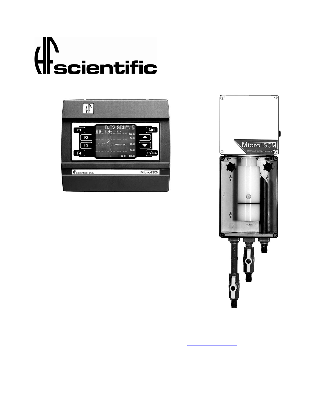
OWNER’S MANUAL
MicroTSCM
Streaming Current
Monitor
HF scientific
3170 Metro Parkway
Ft. Myers, FL 33916
Phone: 239-337-2116
Fax: 239-332-7643
EMail:HFinfo@Watts.com
Website: www.hfscientific.com
21648 (07/09)
REV 2.4
Page 2

Page 3

Table of Contents
Section Page
Specifications ................................................................................................... 1
1.0 Overview........................................................................................................... 2
1.1 Unpacking and Inspection of the Instrument and Accessories ....................2
2.0 Safety................................................................................................................ 2
2.1 Symbols Used In the MicroTSCM........................................................2
3.0 Theory of Operation........................................................................................ 3
3.1 Treatment of Water for Clarification..................................................... 4
3.2 Charge Analysis ....................................................................................5
4.0 Installation and Commissioning ................................................................... 6
4.1 Sample Point ........................................................................................ 6
4.2 Flow Rate .............................................................................................. 6
4.3 Sensor Mounting & Plumbing .............................................................. 7
4.4 Analyzer Mounting................................................................................ 8
4.5 Electrical Connections .......................................................................... 9
4.5.1 Power ........................................................................................ 9
4.5.2 Outputs – Voltage & Current .................................................. 9
4.5.3 Alarm Contacts........................................................................ 10
5.0 Operation ...................................................................................................... 11
5.1 The Sensor/Sampler ...........................................................................11
5.2 The Analyzer ....................................................................................... 11
5.3 The Graphing Screen........................................................................... 12
5.4 Menus ................................................................................................. 13
6.0 Calibration .................................................................................................... 14
6.1 Calibration Procedures ....................................................................... 14
6.2 EEPROM Programming Correction ................................................... 14
7.0 Automatic Control......................................................................................... 15
7.1 Optimization of Treatment Process..................................................... 15
7.2 PI Control Overview ........................................................................... 15
7.3 PI Control Procedure........................................................................... 16
7.3.1 Process Band Calculation........................................................ 16
7.3.2 Entering the Control Parameters ............................................ 17
7.3.3 Manual Control ....................................................................... 17
21648 (07/09)
REV 2.4
Page 4

Table of Contents (continued)
Section Page
8.0 Additional Features and Options ................................................................ 18
8.1 Sensor Gain Switch ............................................................................. 18
8.2 Remote Panel Meter ............................................................................ 18
8.3 Optional Flow Switch.......................................................................... 18
9.0 Routine Maintenance.................................................................................... 19
9.1 Preferred Method – Chemical Cleaning.............................................. 19
9.2 Manual Cleaning ................................................................................. 19
9.3 Analyzer Fuse ..................................................................................... 20
10.0 Troubleshooting............................................................................................. 21
10.1 Diagnostic Chart ................................................................................. 21
10.2 Technical & Customer Assistance ......................................................21
11.0 Accessories and Replacement Parts List .................................................... 22
12.0 Definitions ..................................................................................................... 23
13.0 Warranty........................................................................................................ 24
MICROTSCM (07/09)
REV 2.4
Page 5

Specifications
Measurement Range
Accuracy
Repeatability
Linearity
Resolution
Response Time
Analyzer Display
Alarms
Analog Output
Communications Port
Flow Rate
Flow Alarm
Operating Temperature
Storage Temperature
Wetted Materials
± 10.0 SCU or ICu
±1 % of Full Scale
1%
±1%
0.01 SCU or ICu
1 second
Backlit Graphical LCD with trending
Two Programmable, One Sensor, 120-240VAC 2A Form C Relay
Powered 4-20 mA, 1000 Ω drive
Optional RS-232 or RS-485
6.0 – 9.5.0 L/min. (1.5 -2.5 gpm)
Optional Float Switch
0°C – 50°C (32°F – 122°F)
-20°C – 60°C (-4°F – 140°F)
HDPE, PTFE, Stainless Steel, Neoprene, ABS
Standard Cable Length
Max. Sensor to Analyzer
Power Source
SCM Sensor Case
Analyzer Regulatory
Compliance And
Certifications
Shipping Weight
Shipping Dimensions
Warranty
7.62m (25 feet)
76.25 m (250 feet) Consult factory for lengths over 50 feet
120 or 240 VAC, 50/ 60 Hz, 40VA
Designed to meet IP 66 /NEMA 4X
CE Approved, ETL listed to UL 3111-1 &
ETL Certified to CSA 22.2 No. 1010-1-92
Instrument: 9.5 kg (21 lbs.)
Calibration kit: 5.5 kg (12 lbs.)
Instrument: 61 cm X 46 cm X 35cm (24“ X 18 “ X 14”)
Calibration kit: 41cm X 41 cm X 38 cm (16” X 16” X 15”)
1 Year from date of shipment
MICROTSCM (07/09) Page 1
REV 2.4
Page 6
1.0 Overview
The SCM–Streaming Current Monitor allows for optimizing and control of dosing
coagulants used for clarification of water. Although the analyzer is capable of displaying
the units in either SCU’s or ICu, this manual will always refer to SCU.
1.1 Unpacking and Inspection of the Instrument and Accessories
The table below indicates the items in the shipment.
Item Quantity
MicroTSCM Analyzer 1
SCM Sensor 1
Sample Chamber 1
Calibration Kit 1
Instruction Manual 1
Remove the instrument from the packing carton. Carefully inspect all items to ensure that
no visible damage has occurred during shipment. If the items received do not match the
order, please immediately contact the local distributor or the HF scientific Customer
Service Department.
2.0 Safety
This manual contains basic instructions that must be followed during the commissioning,
operation, care and maintenance of the instrument. The safety protection provided by this
equipment may be impaired if it is commissioned and/or used in a manner not described in
this manual. Consequently, all responsible personnel must read this manual prior to
working with this instrument.
In certain instances “Notes”, or helpful hints, have been highlighted to give further
clarification to the instructions. Refer to the Table of Contents to easily find specific
topics and to learn about unfamiliar terms.
2.1 Symbols Used In the MicroTSCM
Standard IEC symbols are used on the high voltage cover.
ISO 3864, No. B.3.6 Caution, risk of electric shock.
cover
This symbol indicates that hazardous voltages may be present under this
ISO 3864, No.B3.1 Caution refers to accompanying documents.
This symbol is a reminder to read the sections in the manual referring to the
electrical connections, and potential hazards.
MICROTSCM (07/09) Page 2
REV 2.4
Page 7

3.0 Theory of Operation
In a liquid form, water molecules move around each other at a fast rate. One affect of this
fast movement is the ability to suspend matter. This phenomenon is called “Brownian
Motion”. It occurs when microscopic particles are maintained dispersed in suspension due
to their random bombardment by the fast movement of water molecules. Typical particles
found in raw water entering WTP have finely divided clay particles and organic matter
collectively called silt.
A second phenomenon which stabilizes the suspension is the surface charge of the
suspended matter. When a salt such as sodium chloride is place in water, complete
dissolution occurs. This system reaches a stable energy level when the individual sodium
and chloride ions (Na+ and Cl-) are separated in the water phase by being surrounded by
water molecules.
In the case of large pseudo salts, e.g. Aluminosilicates (clay), only partial dissolution takes
place due to incomplete breakdown of the crystal to individual ions. The structure of these
clays is similar to silica or sand except that random silicon atoms in the crystal are
replaced by aluminum atoms in the cage structure, causing the clay to swell and crack
between adjacent aluminum atoms in the crystal. Thus a clay particle is formed with a size
of less than 1 micron with a negative charge. This particle is small enough to be
maintained in suspension by Brownian Motion. The particles in the suspension repel each
other due to their surface charge, preventing them from coming together and
agglomerating, or flocking to form a larger particle, which would settle out. The result is
an energetically stable system and is the reason why the particles remain dispersed.
The counter ions (say sodium for the sake of argument) are separated from the large cage
structure because they are dissolved in the water. Clay particles have a negative charge
associated with it, while the counter ions, typically cat-ions (or positively charged ions)
are dispersed in the water phase.
In the case of most naturally occurring substances, the larger ion, when in suspension, has
a negative net charge (anionic). The smaller, counter ion is positive (cationic). The
residual charge of the larger particles is negative, which causes them to repel each other,
preventing them from forming agglomerates. The size of the particles never becomes large
enough to settle out, so they remain dispersed in suspension.
This phenomenon creates an energetically stable system. In order to cause the suspended
particles to agglomerate and settle out, the energy of the system must be upset. There are
numerous mechanical means to accomplish this, but the addition of chemical flocking
agents to the suspension, drastically reduces the time and is far more efficient.
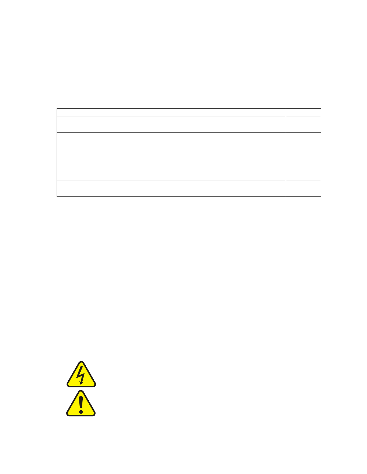
Chemical additives perform two functions, charge neutralization & bridging. Both of these
techniques allow the small particles to floc and grow sufficiently that Brownian motion
can no longer support them. Due to the high density of the particle, flocs will form and
settle as fine sludge.
MICROTSCM (07/09) Page 3
REV 2.4
Page 8
+
-
-
-
-
-
+
+
+
+
+
+
+
+
+
+
-
-
+
-
+
+
-
+
+
+
-
-
-
+
+
+
-
-
-
+
+
-
-
-
-
+
+
+
+
-
+
+
+
+
+
+
-
-
-
-
+
+
+
+
+
+
-
-
-
+
+
-
-
Additive Chemicals
+
-
+
-
-
-
-
-
+
+
-
+
-
+
+
+
Contaminant Particles
1. Charge Neutralization 2. Bridging
Figure 1: Effects of Chemicals
3.1 Treatment of Water for Clarification
Most water treatment chemicals consist of a cationic (positively charged) chemical e.g.
aluminum salts, ferric salts, polyamines or cationic polyacrylamides, some of which have
the cationic part tagged on to a long polymer chain. As stated earlier, raw water entering
the WTP is an energetically stable system of suspended particles with a net negative
charge. Cationic chemicals are added to bring the charge to neutral.
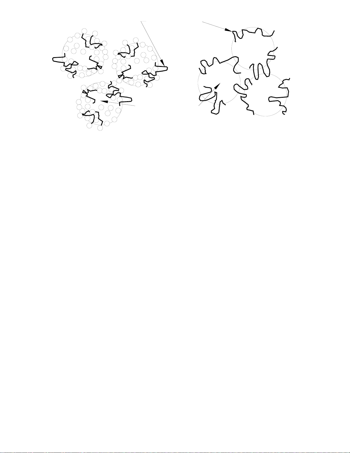
Before the development of Streaming Current technology, the best way to determine the
optimum dosage has been the jar test method. The jar test involves taking a representative
sample of the water being treated and placing it in several jars. Different amounts of
clarifying chemicals are added to each jar; stirred and comparing the clarity of the water in
the different jars. Jar tests are time consuming and it is difficult to reproduce the
conditions of the WTP in a jar. The tests can take several hours rendering them useless
when plant personnel are really responding to rapid changes in water quality. A typical
curve of Turbidity vs. Chemical dosage is shown in Figure 3.
Some considerations when treating the water are the rate of floc formation, the size of the
floc formed, how fast the floc settles, and the clarity of the final settled and filtered water.
Other techniques exist, such as a dosing curve, which indicates a recommended dosage for
a given water turbidity. This is generally built up over years of dosing experience with the
water, but has the disadvantage that turbidity caused by extremely small particles requires
a higher dosage than that caused by larger particles, and therefore can only be adapted for
use with known type turbidity on any given water.
MICROTSCM (07/09) Page 4
REV 2.4
Page 9
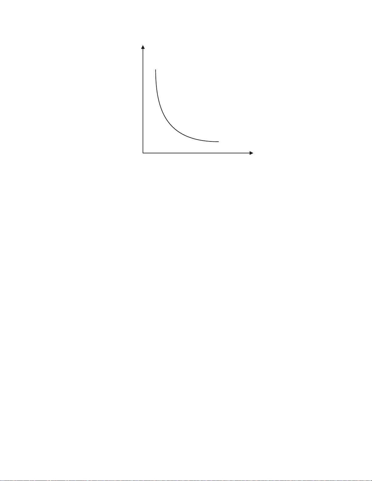
TURBIDITY
CHEMICAL DOSAGE ppm
Figure 3: Turbidity vs Dosage
3.2 Charge Analysis
Charge analysis is the measurement of the electro kinetic charge of a solution due to the
presence of charged particles. The electro kinetic charge can be measured by a number of
different methods.
1. Applied electric field
Measurement: The relative mobility of the solid or liquid phase.
This is the first method developed for calculating the Zeta Potential. The motion of
charged particles under the influence of an electric field was observed and the potential
required to achieve a certain amount of particle mobility was measured.
A cell consisting of two flat plates separated by approximately 0.1 mm and having an
electrode at each end of the cell is filled with water containing suspended matter. When an
electrical potential is applied to the electrodes, the particles can be observed to drift
toward one of the electrodes. The Zeta Potential is calculated from the measured speed of
particle drift.
2. Induced Electrical Potential
Measurement: The potential developed as the result of forced movement of particles in the
solution.
This is the method used by the MicroTSCM. Continuous sample water is directed into an
annulus, inside which a displacement piston oscillates vertically at a fixed frequency. This
action causes the liquid to move between the two stainless steel electrodes. The suspended
particles are absorbed onto the walls under the action of Van der Waal’s and electrostatic
forces. As the sample is moved rapidly back and forth, mobile counter ions surrounding
the colloids are sheared near the surface of the walls and moved past the electrodes. The
resultant A.C. signal or Streaming Current, proportional to charge density, is electronically
processed and displayed.
MICROTSCM (07/09) Page 5
REV 2.4
Page 10

4.0 Installation and Commissioning
4.1 Sample Point
Careful consideration must be given to where in the system the sample will be taken.
Streaming current monitoring requires sampling of the raw water after the introduction of
coagulant. It is critical that that the sample point is far enough from the dosage point to
ensure good mixing. The sample point should be at least 10 pipe diameters away from the
dosing point to ensure ample mixing.
Equally important is the lag time from when a change in dosage occurs to when it shows
up at the sensor. If the sample point is too far from the dosing point, it will take too long
for changes to reach the sensor and control of the loop will not be possible. A lag time not
greater than 10 minutes is recommended.
Figure 3: Typical Installation
4.2 Flow Rate
The absolute minimum flow required is 6 liters per minute (1.5 gpm). The sample is
designed to handle flow rates of up to 10 liters per minute (2.5 gpm). Run the flow as
close to the maximum as possible without overflowing the sample chamber.
Note: The sample flow must be free of large shells or other debris that might clog
the orifices or cause damage to the sensor. Supplying an adequate flow free of
debris is the responsibility of the installer.
Drains MUST be routed to a suitable drain. DO NOT reintroduce this water
back into the process stream.
Suggestion: If meeting the minimum flow rate may be a problem, the optional flow alarm
may be required. HF Catalog #19886. See section 8.3.
To prevent large debris from entering the sample chamber, a 40 mesh screen
strainer is recommended.
MICROTSCM (07/09) Page 6
REV 2.4
Page 11

4.3 Sensor Mounting & Plumbing
Locate the sensor as close to the sampling point as possible to reduce lag time. A site that
is protected from the elements (sun, rain etc.) is preferred, but the sensor is rated for use
under most outdoor conditions. The sample chamber is designed to be mounted with ¼”
diameter bolts. The sensor does not get firmly mounted, but just sits on top of the sample
pot. A light shield protects the clear sample pot cover & helps to prevent algae growth.
Refer to the diagram below for mounting dimensions.
SENSOR ELECTRONICS
THE SENSOR DOES NOT
GET MOUNTED TO THE
WALL. IT INSERTS INTO
THE SAMPLE CHAMBER
AND RESTS ON THE 4
RUBBER BUMBERS.
LIGHT SHIELD
THE LIGHT SHIELD IS USED
TO PREVENT ALGAE
GROWTH INSIDE THE
SAMPLE CHAMBER.
7.09 in
180 mm
10.00 in
254 mm
NOTES:
-THE INSTRUMENT REQUIRES A MINIMUM OF 6 AND A MAXIMUM OF
10 LITERS PER MINUTE CONSTANT FLOW.
-THE DRAIN MUST FLOW FREELY TO AN OPEN DRAIN. ANY
BACKPRESSURE MAY CAUSE THE SAMPLE CHAMBER TO
OVERFLOW.
-THE HOSE BARBS MAY BE REMOVED FOR DIRECT PVC PIPE
CONNECTIONS.
Figure 4: Sensor/Sample Chamber Mounting
STREAMING CURRENT MONITOR
MAIN DRAIN
3/4" HOSE BARB
INLET WATER 3/4"
HOSE BARB
REAR VIEW OF ENCLOSURESAMPLE CHAMBER COVER
1/4 in. (6.35mm) MOUNTING
HOLE (4 PLACES)
OVER-FLOW DRAIN 3/4"
HOSE BARB
7.75 in.
197mm
9.41 in.
239mm
MICROTSCM (07/09) Page 7
REV 2.4
Page 12

4.4 Analyzer Mounting
The analyzer is not weather tight and this must be taken into consideration during site
selection. The analyzer provides the control outputs via 4-20 mA and alarms. It is
recommended that the analyzers be mounted in a location for easy viewing and keypad
access. The analyzer can be flipped on its mount to gain access to the electrical
connections.
Please refer to the drawing below for mounting dimensions and hole location.
Figure 5: Analyzer Mounting
MICROTSCM (07/09) Page 8
REV 2.4
Page 13

4.5 Electrical Connections
All of the electrical connections to the instrument are made at the termination area which
is located in the back of the analyzer under the access cover. Refer to Figure 6 carefully as
the wire colors do not follow the actual PCB screen printing. For easy access, loosen the
two clamping knobs and rotate the instrument upside down. Remove the access cover.
Figure 6: Analyzer Electrical Connections
4.5.1 Power Note: Only qualified electricians should be allowed to perform the installation of the instrument as it involves a line voltage that could endanger life.
The power requirements for the analyzer are 40VA at 120 or 240 VAC. The voltage is set
at the factory based on the shipping destination; however the setting should be checked
prior to power connection.
To change the voltage, the fuse cartridge must be removed and rotated. The voltage is
indicated by the two arrows that point toward each other. A flat bladed screwdriver
inserted into the slot provided may be used to remove the fuse cartridge. See the Figure 11
in section 9.3.
4.5.2 Outputs -Voltage & Current
The analyzer can be set to output either
DISPLAY PARAMETERS menu of the analyzer.
voltage or 4-20 mA. This selection is made in the
Use twisted pair shielded cable 22AWG-14 AWG for the voltage or current outputs. Tie
the shield at the recorder end only. Do not connect the shield at the analyzer.
The voltage connections are made at J6 as shown below:
MICROTSCM (07/09) Page 9
REV 2.4
Page 14

Terminal J6 Connection Purpose Impedance
Terminal 1 0-10V 50K ohm or greater
Terminal 2 0-1V 5K ohm or greater
Terminal 3 0-100 mV 500 ohms or greater
Terminal 4 Common N/A
The 4-20 mA connection is made at J5. Terminal 1 is positive, Terminal 2 is negative. The
recorder load may be up to 1000 ohms.
Galvanic isolation may be achieved by removing the jumper at J13. This procedure will
require the removal of the entire rear cover assembly.
4.5.3 Alarm Contacts
Connections can be made to the two user settable alarms and the sensor alarm at the
terminal block labeled ALARMS.
Note: these alarms are fail safe and will revert to an alarm condition in the event of no
power being applied to the analyzer.
The maximum alarm contact ratings are 250VAC @ 5.0A. Ensure that loads do not
exceed these ratings.
As indicated on the PCB, the following are terminal blocks:
J1 – Alarm 1
J2 – Alarm 2
J3 – Alarm 3
In all cases the following connections apply:
Terminal 1: Normally Closed (N.C)
Terminal 2: Normally Open (N.O.)
Terminal 3: Common (C)
Do not use wire larger than #14 AWG as the terminal blocks will not accept it.
MICROTSCM (07/09) Page 10
REV 2.4
Page 15

5.0 Operation
The SCM system consists of three major components, The Sensor, the Sample Chamber
and the Analyzer.
5.1 The Sensor/Sample Chamber
The sensor module sits on top of the sample chamber, with the probe end below the water
level. The sample chamber has three valves to adjust the flow:
• The inlet should be adjusted such that there is always a sample present. A lack of
a sample will cause premature wear in the cell and piston.
• The main drain needs to be adjusted open as much as possible to allow the larger
particulates to drain while the sample water is measured.
• The overflow valve is usually connected to the main drain and is left fully open.
Its purpose is to keep the sample chamber from overflowing.
To prevent back flow and allow proper draining it is important that both drains are left
open to the atmosphere and kept at short as possible.
If heavy particulates can be present in the water it is important to install a 40 mesh strainer
before the inlet. The flow should also be kept low to allow large sand and larger debris to
fall to the bottom of the sample chamber and drain, without causing harm to the sensor.
The sample chamber has a cover to reduce algae growth. This cover may be easily
removed for service.
5.2 The Analyzer
Detail is not provided on individual menus as most are self explanatory. Notes are used,
where needed to bring attention to important information.
There are a few analyzer keys which have special purposes as described below.
This key resets the alarms after an alarm condition has been met. A screen
display of the alarm will continue until the alarm condition is relieved.
Alarms will also reset themselves without intervention if instrument
reading returns to a non- the alarm condition.
The Enter/Menu key is used to either invoke the Main Menu while in the
graphing screen or to return to the previous menu.
These two buttons are used to modify values or to scroll through possible
selections.
MICROTSCM (07/09) Page 11
REV 2.4
Page 16

5.3 The Graphing Screen
Shown below in Figurer 7 is the main graphing screen. The numbers are used to identify
various features.
1. The larger number area shows the current reading and units used.
2. The graph time base. Options are 8 or 24 hours and can be set in the Display
Parameters Menu.
3 & 4. The upper and lower display limits. These are settable in the Display Parameters
Menu. Please note that these settings also affect the 4-20 mA /Voltage range.
5 & 6. Alarms 1&2. These can be set in the Alarms Setup Menu. These will flash on the
graphing screen if in an alarm condition.
7 & 8. Current time & date. This can be set in the Monitor Setup Menu.
9. Streaming current graph.
Figure 7: Analyzer Screen
MICROTSCM (07/09) Page 12
REV 2.4
Page 17

5.4 Menus
The following flow chart can be referred to for the menu structure.
Figure 8: Menu Flow Chart
MICROTSCM (07/09) Page 13
REV 2.4
Page 18

6.0 Calibration
The MicroTSCM has been calibrated at the factory, however to ensure accuracy it is
recommended that the instrument be calibrated prior to being placed online. Long term
drift may occur in this instrument and HF scientific recommends calibration every three
months.
To facilitate the initial calibration, a calibration kit, Part # 19922 is supplied with this
instrument. When prepared according to the included instructions a +5.30 SCU Cationic
calibration solution is produced. Allow this solution to stand for one hour prior to use.
In preparation for calibration ensure that previously operated sensors are rinsed with, and
then operated in, clean water, for several minutes.
6.1 Calibration Procedures
Place the sensor in the Cationic Standard and allow it to stand for about 15 minutes.
Ensure that the gain switch is set to OFF. See section 8.1
On the Analyzer ensure that the Offset Level is set to 0.00 and the signal averaging is
turned OFF. To calibrate, on the Analyzer, go to Sensor Setup → Extended Setup → Full
Scale Cal. → Cal Time. The S key will initiate the calibration, which will take 60
seconds.
At the completion of the calibration, ensure that the reading is +5.10 to +5.50 SCU. If the
reading appears unstable initiate another calibration. If the +5.30 SCU calibration value is
not achievable, refer to section 6.2.
Rinse the sensor with clean water prior to returning to service.
As a check, an Anionic solution can be made using a 100mg/l dishwater detergent
solution. An acceptable reading would be -4.0 to -6.0 SCU.
Note: Do not attempt to calibrate on an Anionic solution.
6.2 EEPROM Programming Correction
If the calibration in the Cationic solution does not achieve a reading of +5.10 to +5.50
SCU, the EEPROM has probably lost the storage value and will need to be reprogrammed.
This will need to be performed at the sensor while operating in the calibration solution.
Remove the sensor cover by loosening the four corner captive fasteners. Inside locate a
small DIP switch with four white sliders labeled SW4. Above this switch are two push
buttons labeled SW2 and SW3. On the DIP switch flip the slider labeled 3 up. The
analyzer should display +5.30. If it does not adjust the value with the push buttons; SW2
will increase the value (UP) SW3 will decrease the value (DOWN). Adjust until the
Analyzer reads exactly +5.30 SCU. Flip the slider on the DIP switch down to store the
adjustment.
Attempt another calibration from the Analyzer as in section 6.1. If the correct calibration
values are still not achievable, call HF scientific Technical Service Department for
assistance.
MICROTSCM (07/09) Page 14
REV 2.4
Page 19

7.0 Automatic Control
This section describes the use of the SCM to control the process. It is recommended that a
review of section 4.1 (sample point) is made to ensure correct installation.
7.1 Optimization of Treatment Process
Prior to turning control over to the SCM, it is crucial to optimize coagulant dosing. The
optimum point is obtained when the minimum coagulant can be fed that produces the
desired results for any particular treatment process. This should be done slowly and in
steps.
Step 1: Track the water quality parameters over the course of several days to establish a
base line of data from which to measure acceptable water quality.
Suggestion: The Installation Evaluation format the back of this manual is a tool that can
be used to track water quality parameters.
Step 2: After the base line of acceptable water quality has been reached, reduce the
coagulant dosage by 5% and closely monitor the water quality.
Step 3: Continue reducing the dosage in 5% increments until there is a detectable
reduction in water quality. Increase the dosage from this point by 5% and
continue monitoring for another hour.
Step 4: Record the SCU value on the instrument as this will be the optimized set point
(SP) for operating the plant.
Note: There may be a different set point for extreme variations in raw water quality or
demand on the system e.g. winter versus summer.
7.2 PI Control Overview
The MicroTSCM can be incorporated into an existing control scheme using the 4-20mA
or serial outputs. Plant control can also be achieved using the optional Proportional
Integral feature included in the MicroTSCM analyzer (HF Catalog # 19550 only).
When the instrument is used to automatically control coagulant dosing, it monitors the
process value (PV) for a change in charge value and then adjusts the dosage up or down to
achieve the predetermined set point (SP). Using a control algorithm or process calculation,
the analyzer determines the pump speed that is required to keep the PV and SP values the
same, which is the function of any closed loop control system.
When placed under automatic control, the instrument performs the same tasks that an
operator would be required to make. An operator adjusts the dosage level, allows time to
account for mixing and then checks the process for the desired change. Additional changes
to the dosage level are made as required. Under automatic control, the instrument
constantly monitors the process value and makes adjustments as needed to maintain the
process reading at the set point.
In order to put the plant under automatic control, it is required to provide some basic
information to the analyzer that describes how the system responds to changes. The
variables that need to be determined are the Proportional Band and the Integral Time. The
Proportional Band tells the instrument what change in Streaming Current to expect for a
MICROTSCM (07/09) Page 15
REV 2.4
Page 20

given change in coagulant dosing. The Integral Time tells the instrument how long it will
take to fully realize the effects of a change in coagulant dosing.
7.3 PI Control Procedure
The assumption is that the wiring between the MicroTSCM analyzer and the dosing pump
has been installed. The following procedure is recommended to determine the correct
Proportional - Integral (PI) values for any particular system. The MicroTSCM analyzer is
used to slow down the control loop to prevent overdosing of coagulant. A calculation
based on test data determines the Proportional Band or P. Band and is the final value that
will be entered into the analyzer. A hypothetical example of the procedure will be used to
demonstrate the calculation of these values. These values will need to be determined for
any particular system and can be plugged into the following equations to determine the
appropriate analyzer settings.
Steps:
1. Ensure the plant is operating at a steady SCU reading with a fairly constant flow
rate. Record this SCU value.
2. Adjust the dosing pump to give a 10% increasing dosing output.
3. Start timing when the change was made (a stopwatch is helpful).
4. Monitor the MicroTSCM and stop timing when the SCU value has changed and
leveled off.
5. Record this time period in seconds. This is the Integral Time setting.
6. Record the new SCU value when the change has fully leveled off.
Figure 9: Effect of Dosing Change
7.3.1 Proportional Band Calculation
For our hypothetical example, the cause of change was the 10% increase in pump output
i.e. 10% more coagulant was dosed into the water. Due to the requirement to mix the
coagulant with the carrier water and move it through the volume of the sample pot, we
observed a time lag. The total time from when the change was made to when the full
effect was noticed was 100 seconds. This will be entered later as the Integral Time (INT.
TIME). The SCU reading changed was from -2.5 SCU to -2.0 SCU; a change of 0.5 SCU.
MICROTSCM (07/09) Page 16
REV 2.4
Page 21

Convert the effected change in SCU to a percentage. Since the instrument always operates
in a range of +10 SCU to -10 SCU, the range is 20 SCU.
% effect = Effect X 100
Range 1
Then calculate the proportion band or PB.
PB = % Effect X 100
% Cause 1
In our example calculating the Proportional Band or P. Band with a 10% change (cause):
% effect = 0.5 SCU X 100 = 2.5%
20.0 SCU 1
PB = 2.5%
10% 1
To prevent overshoot, it is desirable to slow the control loop down a little more. To do this
the PB is multiplied by 1.5.
In our example:
X 100 = 25%
PB = 25% X 1.5 ≈ 38%
Once the control parameters are set into the analyzer and the dosing pump has been set,
the SP may need to be adjusted to account for seasonal change, but other than routine
maintenance and monitoring, no other adjustments should be required.
7.3.2 Entering the Control Parameters
The next step is to enter the control parameters into the MicroTSCM analyzer. To do this,
follow the steps:
1. Press /Menu to enter the Main Menu screen.
2. Press F1 (Sensor Setup) to enter the Sensor Setup screen.
3. Press F4 (Extended Setup) to enter the Extended Setup screen.
4. Press F2 (PID Analyzer) to enter the PID Analyzer screen.
5. At F1 (Mode) toggle the highlighted setting to AUTO using the STbuttons.
6. Press F3 (Set Point) adjust the Set Point (from section 7.1) using the STbuttons.
7. Press F4 (P. BAND) adjust value using the STbuttons (in our example 38.00).
8. Press F4 again (INT. TIME) adjust value using the STbuttons (in our example 100).
9. Press /Menu four times to return to the graphic monitoring screen.
7.3.3 Manual Control
To operate the system in manual mode, follow the steps 1-4 above, on step 5 use the
STbuttons to adjust the setting to MANUAL. Select F2 and a new setting called
MANUAL OVERRIDE will show. Adjust the value using the STbuttons. A +10 will
increase the pump speed by 10% and -10 will decrease pump speed by 10%. Please note
that the speed change may not be representative of dosing rate.
MICROTSCM (07/09) Page 17
REV 2.4
Page 22

8.0 Additional Features and Options
8.1 Sensor Gain Switch
The gain toggle switch is mounted on the side of the sensor housing. The purpose of the
gain switch is to increase the magnitude of the sensor’s response. The gain switch can be
used in applications where little response is noted to changes in coagulant dosing. When
deciding to use the gain switch try the LOW setting first. If the response is not adequate,
use the HIGH setting. Always be sure this switch is turned to OFF (center position) when
calibrating.
As increasing the gain may over-range the reading, this feature should not be used unless
the reading is near zero.
8.2 Remote Panel Meter (Catalog # 19609)
The optional remote panel meter allows for remote indication of the SCU reading using
the 4-20 mA loop of the MicroTSCM. No external power is required, as the meter is
powered from the 4-20 mA source of the MicroTSCM analyzer.
8.3 Optional Flow Switch (Catalog # 19886L)
The flow switch is actually a float level switch. This is a factory installed option that will
alert an operator to a lack of flow. Once actuated a low flow condition will be indicated on
the screen as well as sending the 4-20 mA signal to ground and closing the alarm contacts.
There is a user setting in the analyzer to determine how long a lack of flow is required to
initiate an alarm.
MICROTSCM (07/09) Page 18
REV 2.4
Page 23

9.0 Routine Maintenance
The most important maintenance procedure is to keep the sensor clean. The need for
cleaning is indicated when normal readings cannot be maintained. As a preventative
measure, cleaning intervals of 30 days or less is recommended. There are two
recommended cleaning methods.
9.1 Preferred Method – Chemical Cleaning
Pour the SCM-1 cleaning solution (Catalog # 19402) into a suitable container, large
enough to immerse the lower 1/2 of the probe body. Run the sensor in this solution for
approximately 10 minutes. Then run the instrument for about 10 minutes in clean water.
For organic debris, replace the cleaning solution with a 5% chlorine solution.
Please refer to the Material Safety Data Sheet for proper handling of the SCM-1 cleaning
solution.
9.2 Manual Cleaning
In extreme conditions, the cell will have to be removed and cleaned with an abrasive
cleaning pad such as Scotch-Brite® and a small brush.
Always rinse the probe out with clean water prior to starting.
1. To expose the cell and probe area, remove the bottom cap by turning it CCW (as
viewed from the bottom). Be careful to retain o-rings and seals.
2. Carefully pull the Cell out of the probe end, about 25-50 mm (1-2 inches)
3. Clean the inside of the cell with a stiff toothbrush and an abrasive pad such as
(Scotch-Brite®). The aim is to remove all debris and polish all stainless steel
surfaces.
4. Rinse the cell with water.
5. Loosen the shaft-retaining nut with a 10mm wrench and from the bottom of the
sensor unscrew the probe.
6. Completely remove the nut then pull the probe out.
7. Polish the probe with the abrasive pad.
8. Reinstall the probe, adjusting the probe such that it misses the bottom of the cell by
1-2 mm, then snug the 10mm retaining nut. DO NOT OVER-TIGHTEN.
9. Completely dry off any water that is in and around the cell cap, the bottom of the
cell and the O-rings and seals.
10. Reassemble the lower seals and install the cap very firmly by hand.
11. Rotate the motor slowly by hand to ensure the probe does not hit the cell bottom. If
there appears to be any contact adjust the probe up slightly.
12. If the probe does not rotate freely inside the cell, check for obstructions. This
condition will cause premature motor wear.
MICROTSCM (07/09) Page 19
REV 2.4
Page 24

Figure 10: Sensor – Exploded View
9.3 Analyzer Fuse
The analyzer fuse located in a cartridge on the cord
receptacle in the back of the instrument. To gain access,
remove the four access cover screws and remove the
power cord. Insert a screwdriver into the slot and pry to
remove the cartridge. Be certain to match the desired
voltage with the indication arrow when reinserting the
cartridge.
Figure 11: Fuse
MICROTSCM (07/09) Page 20
REV 2.4
Page 25

10.0 Troubleshooting
10.1 Diagnostic Chart
Symptom Solutions
Analyzer Display Not Lit. 1. Make sure the unit is plugged in and turned on.
2. Make certain that the power source is providing the
correct voltage.
3. Make sure the analyzer is set for the correct voltage.
4. Check analyzer fuse.
Sensor probe not moving 1. Check the interconnect cable connection at the sensor.
2. Check the wiring of the interconnect cable on the back
of the analyzer and inside the sensor.
3. Check to ensure the probe is not jammed.
Display Response is Slow 1. Select a lower Signal Averaging period.
2. Separation between dosing and sample points too great.
Readings Different than expected 1. Sensor requires cleaning.
2. Sensor requires calibration.
3. Check Probe and Cell for wear. Replace parts as
required.
Unable to Achieve 5.3 SCU after
Calibration
Sensor Alarm Indication on
Analyzer
Reading Fluctuate, Unstable 1. Incomplete mixing of coagulant with sample water.
Reading Doesn’t Change with a
Change in Dosing
10.2 Technical and Customer Assistance
If for any reason assistance is needed regarding this instrument please do not hesitate to
contact either the HF scientific Service Department or the HF scientific Customer Service
Department.
1. Manually reprogram calibration as described in section
6.2 EEPROM Programming Correction.
1. Check that sensor is operating correctly.
2. Check wiring connections at both the analyzer and the
sensor.
2. Sensor and or sample chamber require cleaning.
3. Check coagulate dosing operation.
1. Sensor may require cleaning.
2. Check sample flow to sample chamber.
3. Ensure complete coagulant mix with water.
MICROTSCM (07/09) Page 21
REV 2.4
Page 26

11.0 Accessories and Replacement Parts List
The items shown below are recommended accessories and replacement parts.
Accessory Catalog Number
Cleaning and Descaling Solution 19402
Optical Isolated RS-485 Interface Kit 20519
RS-232 Interface Kit 19861
Flow Alarm 19886
Calibration Kit 19922
Interconnect Cable 7.6 meter (25 Ft.) 22480
Operating & Maintenance Manual 21648
To order any accessory or replacement part, please contact the HF scientific Customer
Service Department. If for any reason technical assistance is needed regarding this
instrument, please do not hesitate to contact the HF scientific Service Department.
HF scientific
3170 Metro Parkway
Fort Myers, Florida 33916-7597
Phone: (239) 337-2116
Fax: (239) 332-7643
Email: HFinfo@Watts.com
www.hfscientific.com
MICROTSCM (07/09) Page 22
REV 2.4
Page 27

12.0 Definitions
Anionic: Negative charged ions.
Automatic Control: Placing the control of the dosing pumps under the control of the
Brownian Motion: A phenomenon which occurs when microscopic particles are
Cationic: Positive charged ions.
ICu: Ion Charge unit. 1 ICu is approximately equal to 1 mA of charge.
Ion Charge
Analyzer: Another name for a Streaming Current Monitor.
PI Control: Proportional Integral Control .A process control algorithm that
PID Control: Proportional Integral Differential Control. A higher level control
Silt: A collective of finely divided clay particles and organic matter
Zeta Potential: The charge potential required to induce particle mobility when
SCU: Steaming current unit. 1 SCU = 1ICu.
Streaming current monitor. The Optional PI controller is
recommended.
suspended in a solution due to their random bombardment by the
fast movement of water molecules.
1 ICu = 1 SCU.
allows for a faster, tighter control.
algorithm than PI control, but not required in Streaming Current
applications.
suspended in water.
placed under the influence of an electric current.
MICROTSCM (07/09) Page 23
REV 2.4
Page 28

13.0 Warranty
HF scientific, as vendor, warrants to the original purchaser of this instrument that it will be
free of defects in material and workmanship, in normal use and service, for a period of one
year from date of delivery to the original purchaser. HF scientific’s, obligation under this
warranty is limited to replacing, at its factory, the instrument or any part thereof. Parts,
which by their nature are normally required to be replaced periodically, consistent with
normal maintenance, specifically reagent, desiccant, sensors, electrodes, tubing and fuses
are excluded. Also excluded are accessories and supply type items.
Original purchaser is responsible for return of the instruments, or parts thereof, to HF
scientific’s factory. This includes all freight charges incurred in shipping to and from HF
scientific’s factory.
HF scientific is not responsible for damage to the instrument, or parts thereof, resulting
from misuse, environmental corrosion, negligence or accident, or defects resulting from
repairs, alterations or installation made by any person or company not authorized by HF
scientific.
HF scientific assumes no liability for consequential damage of any kind, and the original
purchaser, by placement of any order for the instrument, or parts thereof, shall be deemed
liable for any and all damages incurred by the use or misuse of the instruments, or parts
thereof, by the purchaser, its employees, or others, following receipt thereof.
Carefully inspect this product for shipping damage, if damaged, immediately notify the
shipping company and arrange an on-site inspection. HF scientific cannot be responsible
for damage in shipment and cannot assist with claims without an on-site inspection of the
damage.
This warranty is given expressly and in lieu of all other warranties, expressed or implied.
Purchaser agrees that there is no warranty on merchantability and that there are no other
warranties, expressed or implied. No agent is authorized to assume for HF scientific, any
liability except as set forth above.
HF scientific, inc.
3170 Metro Parkway
Fort Myers, Florida 33916-7597
Phone: (239) 337-2116
Fax: (239) 332-7643
Email: HFinfo@Watts.com
Website:www.hfscientific.com
MICROTSCM (07/09) Page 24
REV 2.4
Page 29

HF scientific
Installation Evaluation
Use this worksheet to help establish a baseline for optimal dosing. Readings every 6 hours
are recommended.
Date
and
Time
pH
Before
Dosing
Additional Notes:
pH After
Clarification
Turbidity
Before
Clarification
Turbidity
After
Clarification
Color
Before
Dosing
Color After
Clarification
Target
Dosing
Level
Flow
Rate
(gpd)
Page 30

 Loading...