HEKA EPC 9 User Manual

8.52
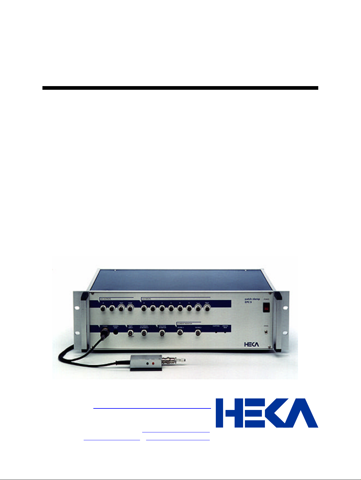
EPC 9 Manual

HEKA Elektronik Dr. Schulze GmbH

Wiesenstraße 71 • D-67466 Lambrecht • Germany

Tel: [phone] • Fax: [phone]

Web Site: http://www.heka.com

E-mail:

[email protected] •

[email protected]

Table of Contents

1. Introduction 5

Introducing the EPC 9 _____________________________________________ 5
References ____________________________________________________ 6
Naming Conventions______________________________________________ 8

EPC 9, EPC 9 Double, and EPC 9 Triple................................................................................... 8

Windows versions ................................................................................................................ 8

Support Hotline _________________________________________________ 9

2. Description of the Hardware 10

Probe _______________________________________________________ 10
Main Unit_____________________________________________________ 11
EPC 9 Double and Triple __________________________________________ 15

3. Installation 16

Installation Procedure ____________________________________________ 16
Calibrating the EPC 9 ____________________________________________ 16
Creating the C-fast Lookup Table_____________________________________ 18

4. Verifying and Testing the EPC 9 19

Testing the EPC9 with the Model Circuit ________________________________ 19

The Model Circuit MC 9....................................................................................................... 19

Step 1: Applying the Test Pulse.............................................................................................20

Step 2: ”On-Cell” Voltage-Clamp Recording.............................................................................23

Step 3: ”Whole-Cell” Voltage-Clamp Recording ........................................................................ 24

Step 4: ”Whole-Cell” Current-Clamp Recording.........................................................................26

Step 5: Measuring the Noise of the Amplifier............................................................................29

Making a ”Full Test” _____________________________________________ 31
Measuring the Frequency Response __________________________________ 34

Table of Contents EPC9 Manual 2

5. E9SCREEN Software 35

EPC9 Window _________________________________________________ 35

Main Controls.................................................................................................................... 35

Hidden Controls................................................................................................................. 46

Notebook Window_______________________________________________ 48
Drop-Down Menus ______________________________________________ 48

File Menu .........................................................................................................................48

Edit Menu......................................................................................................................... 49

EPC9 Menu ......................................................................................................................50

Notebook Menu ................................................................................................................. 52

Calibrate Menu .................................................................................................................. 53

6. Operating Modes 54

Voltage-Clamp Mode _____________________________________________ 54
Current-Clamp Mode _____________________________________________ 54
Test Mode ____________________________________________________ 57
Search Mode __________________________________________________ 58

7. Compensation Procedures 59

Series Resistance Compensation ____________________________________ 59
Capacitance Compensation ________________________________________ 62
Offset Compensation_____________________________________________ 63

8. Patch-Clamp Setup 67

Mounting the Probe ............................................................................................................ 67

Ground Wires.................................................................................................................... 67

Grounding the Microscope ................................................................................................... 67

External Shielding .............................................................................................................. 68

Connections to other Instruments .......................................................................................... 68

Pipette Holder and Electrode ................................................................................................ 68

Bath Electrode...................................................................................................................69

9. Patch-Pipettes 71

Glass Capillaries................................................................................................................ 71

Pulling..............................................................................................................................72

Table of Contents EPC9 Manual 3

Coating ............................................................................................................................ 72

Heat Polishing ................................................................................................................... 73

Use of Pipettes .................................................................................................................. 73

10. Using the Patch Clamp 75

Forming a Seal_________________________________________________ 75

Initial Setup.......................................................................................................................75

Entering the Bath ............................................................................................................... 75

Forming a Gigaseal ............................................................................................................76

Cell-Attached Recording __________________________________________ 76
Whole-Cell Recording ____________________________________________ 77

Breaking the Patch ............................................................................................................. 77

Capacitive Transient Cancellation..........................................................................................78

Series Resistance Compensation .......................................................................................... 78

Current-Clamp Recording__________________________________________ 79

11. Low-Noise Recording 80

Appendix I: Controlling E9SCREEN 83

Communication between E9Screen and other Programs _____________________ 83

Reserving the AD/DA-board for exclusive use .......................................................................... 83

The “EPC9out.EPC” file.......................................................................................................83

Controlling the EPC9 from another Program _____________________________ 85

Sending Commands to E9Screen.......................................................................................... 85

Error Messages..................................................................................................................87

Implemented Commands and Messages.................................................................................87

Notes to Programmers.........................................................................................................91

Sample program ................................................................................................................93

Appendix II: Technical Data 98

Digital I/O Connector_____________________________________________ 98

Standard EPC9..................................................................................................................98

EPC9 Double and Triple ...................................................................................................... 99

Index 101

Table of Contents EPC9 Manual 4

1. Introduction

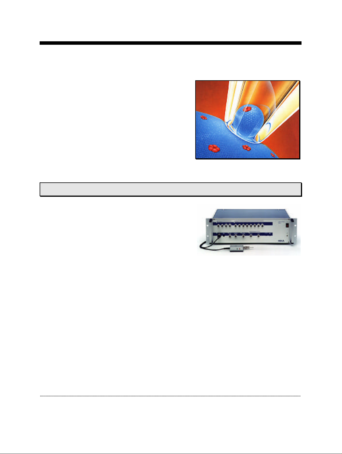
The patch-clamp technique was introduced by
Neher and Sakmann (1976) for recording the
currents in a small patch of membrane under
voltage-clamp conditions. In the intervening
years a number of changes have occurred, most
notably the development of the “gigaseal” by E.
Neher (1981). Various recording configurations
allow intracellular recordings to be made with
the same type of recording setup as used for
patch recording from the cell surface or cell-free
membrane patches (Hamill et al., 1981).

Introducing the EPC 9

The EPC9 represents roughly the ninth in the
series of patch-clamp designs in use in the
Göttingen laboratories. It is a logical successor to
the EPC7, retaining all of its features but adding
a number of capabilities, the most important
being implementation of full digital control of
the various functions. Thus, the new digitally
controlled EPC9 patch-clamp amplifier has no knobs, switches or dials. The Pulse
software replaces the analog controls of conventional amplifiers by using Macintosh
computers and a built-in ITC-16 interface. The convenient graphics display and
mouse operations provide unsurpassed versatility and ease of operation.

In addition to the controls for the amplifier and the built-in filters, the Pulse software
contains a powerful data acquisition system (sampling and storage in pulse, ramp
and continuous modes), a fully programmable pulse generator, and a digital
oscilloscope. Thus, the EPC9 offers all the features of a complete workstation for
controlling experiments and acquiring data. Furthermore, there is the PulseFit
software package as well as TAC (Threshold Analysis for single Channels) available,
which allow data analysis, data export, and graphics output.

The EPC9 also accepts a stimulus input and provides current monitor outputs just
like conventional amplifiers to operate in combination with a host computer running
custom and commercial software from other sources. The versatility of the EPC9 can

Introduction EPC9 Manual 5

best be appreciated by the variety of experiments that can be carried out with it.
Besides high-resolution recordings of single channels, it can be used in studies of
whole-cell voltage and current clamp, exocytosis (by monitoring changes in cell
membrane capacitance), and recordings from artificial membranes or loose-patch
experiments. Technically, the EPC9 is noteworthy for three special features, the
range-changing capability of the head stage, the extremely wide bandwidth available
from the current monitor circuitry, and the integrated transient cancellation
(automatically if desired) and series-resistance compensation functions. Together
these features mean that a single head stage suffices for both single-channel and
whole-cell recordings, and that both kinds of recordings can be made with high time
resolution and low noise.

This manual is designed to provide a general guide for setting up and using the
EPC9 for experiments. It covers general information about the hardware, the
E9Screen program, and basic principles o f the EPC9's functions and patch-clamp
techniques.

It is assumed that the reader has some familiarity with patch-clamp techniques;
should you be a newcomer to the field perhaps the best place to start would be the
paper by Hamill et al., where the basic gigaseal techniques are described and the first
three chapters of Single Channel Recording (B. Sakmann & E. Neher, eds., Plenum
Press, New York, 1995). Certainly, it will be worthwhile to read this manual
carefully. Many users will want to read some of the more advanced and complete
discussions of individual topics which can be be found in original articles and in the
books Single Channel Recording (B. Sakmann & E. Neher, eds., Plenum Press, New
York, 1995) and Methods in Enzymology, vol. 207 (Academic Press, New York, 1992).

References

Original Articles

Hamill, O. P., Marty, A., Neher, E., Sakmann, B. & Sigworth, F. J. (1981) Improved
patch clamp techniques for high-resolution current recording from cells and cell-free
membrane patches. Pflügers Arch. 391, 85-100.

Neher, E. (1981) Unit conductance studies in biological membranes. In: Techniques in
Cellular Physiology (P. F. Baker, ed.) Elsevier/North Holland.

Neher, E. & Sakmann, B. (1976) Single-channel currents recorded from membrane of
denervated frog muscle fibres. Nature 260, 779-802.

Introduction EPC9 Manual 6

Rae, J. & Levis, R. (1984) Patch clamp recordings from the epithelium of the lens obtained
using glasses selected for low noise and improved sealing properties. Biophys. J. 45, 144-

146.
Barry, P. H. & Lynch, J. W. (1991) Liquid junction potentials and small cell effects in

patch-clamp analysis. J. Memb. Biol. 121, 101-117.
Sigworth, F. J., Affolter, H. & Neher, E. (1995) Design of the EPC-9, a computer-

controlled patch-clamp amplifier. 2. Software. J. Neurosci. Methods 56, 203-221.
Book Chapters

Penner, R. (1995) Chapter 1: A practical guide to patch clamping. In: Single-Channel
Recording (B. Sakmann & E. Neher, eds.) Plenum Press, New York.

Marty, A. & Neher, E. (1995) Chapter 2: Tight-seal whole-cell recording. In: Single­Channel Recording (B. Sakmann & E. Neher, eds.) Plenum Press, New York.

Heinemann, S. H. (1995) Chapter 3: Guide to data acquisition and analysis. In: Single-
Channel Recording (B. Sakmann & E. Neher, eds.) Plenum Press, New York.

Sigworth, F. J. (1995) Chapter 4: Electronic design of the patch clamp. In: Single Channel­Recording (B. Sakmann & E. Neher, eds.) Plenum Press, New York.

Neher, E. (1995) Chapter 6: Voltage offsets in patch-clamp experiments. In: Single
Channel-Recording (B. Sakmann & E. Neher, eds.) Plenum Press, New York.

Colquhoun, D. & Sigworth, F. J. (1995) Chapter 19: Fitting and statistical analysis of
single-channel records. In: Single-Channel Recording (B. Sakmann & E. Neher, eds.)

Plenum Press, New York.
Neher, E. (1992) Correction for liquid junction potentials in patch clamp experiments. In:

Methods in Enzymology 207, 123-131, Academic Press, New York.

Introduction EPC9 Manual 7

Naming Conventions

EPC 9, EPC 9 Double, and EPC 9 Triple

Throughout the present manual we will address all three amplifier types as “EPC9”.
We will explicitly mention the particular amplifiers, where it is required.

Windows versions

The EPC9 is supported on Windows 3.1, Windows 95, Windows 98,
Windows NT 3.51, Windows NT 4.0, and Windows 2000.

Throughout the present manual we will address all the above Windows versions as
“Windows”. We will explicitly mention the particular Windows versions, whenever
it is required.

Introduction EPC9 Manual 8

Support Hotline

If you have any question, suggestion, or improvement, please contact HEKA’s
support team. The best way is to send us an e-mail or fax specifying:

• Your postal and e-mail address (or fax number)

• The program name:

E9SCREEN, PULSE, PULSEFIT, etc.

• The program version number:

v8.31, v8.50

• Your operating system and its version:

MacOS 7.6.1, MacOS 8.5,
Windows 98, Windows NT 4.0, etc.

• Your type of computer:

Mac PPC 8500, Pentium II 300 MHz, etc.

• Your acquisition hardware, if applicable:

EPC9, ITC–16, ITC–18

• Your amplifier, if applicable:

EPC9, EPC9 Double, Axon 200B, etc.

• The serial number and version of your EPC9, if applicable:

EPC9 single, version “920552 D”.

• The questions, problems, or suggestions you have

• Under which conditions and how often the problem occurs

We will address the problem as soon as possible.

HEKA Elektronik GmbH phone: [phone]
Wiesenstrasse 71 fax: [phone]
D-67466 Lambrecht/Pfalz e-mail: [email protected]
Germany web: http://www.heka.com

Introduction EPC9 Manual 9

2. Description of the Hardware

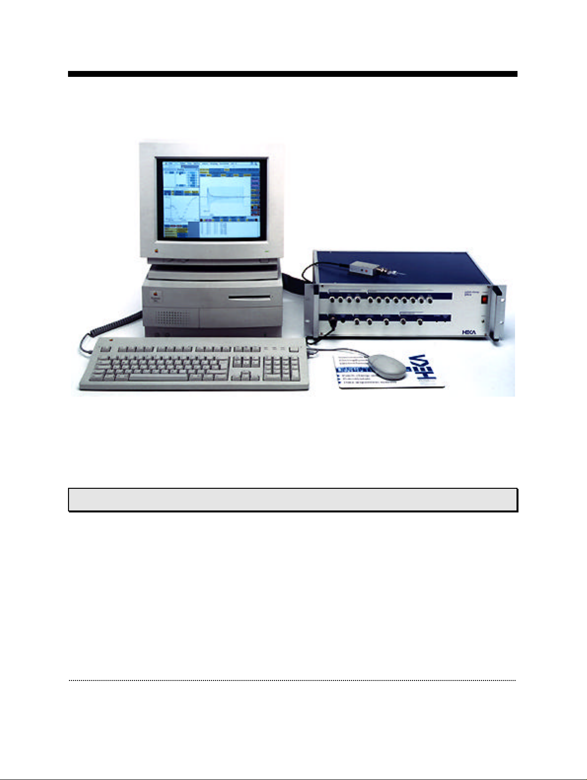
The hardware components of the EPC9 patch-clamp system consist of the head stage
(or probe), the amplifier main unit with the integrated ITC-16 interface board, and
the computer system. Specific information about the hardware installation is given
below in Chapter 3. Installation on page 16.

Probe

The probe, or “head stage” of the EPC9 is contained in a small enclosure designed to
be mounted on a micromanipulator and directly attached to the recording
micropipette. It contains the sensitive amplifier that constitutes the current-to­voltage converter, as well as components for injecting test signals into that amplifier.
On the probe are the following connectors:

Input Connector: This is a Teflon-insulated BNC connector. The standard pipette
holder plugs directly into this connector; the center pin is the amplifier input, and
the shield is driven with the command potential Vp.

Description of the Hardware EPC9 Manual 10

Note: Avoid touching the probe's input terminal, since the input circuitry of the probe can

be damaged by static electricity. When it is necessary to touch the input (e.g., while
inserting a pipette into the holder), ground yourself first by touching a grounded
metal surface.

Ref Output: The red 0.04" pin jack carries the command potential Vp.

Note: The metal case of the probe is also connected to this signal, and therefore must be

insulated from ground.

Gnd Connector: The black pin jack carries a high quality ground signal which is
useful for grounding the bath electrode and nearby shields without potential errors
that could arise from ground loops. This ground is connected directly to the signal
ground on the controller through the probe's cable. More details on grounding
practices will be provided in Chapter 8. Patch-Clamp Setup on page 67.

Main Unit

The main unit of the EPC9 contains the power supply, the signal processing
electronics, the AD and DA converters and the connectors for analog and digital
input/output. Essentially all of the calibration adjustments are made by digital
switches in the main unit, including those which depend on the properties of
components in the probe. The calibration parameters are preset by the manufacturer
and contained in the software package as the files “Scale.epc” and “CFast.epc”.
Unlike conventional amplifiers, hardware calibration of the EPC9 can also be
performed by the user if necessary (see section Calibrating the EPC 9 on page 16).

Note: Calibration parameters are unique to each amplifier and head stage combination.

Thus, if you exchange the head stage, be sure to perform a new hardware calibration.

Voltage Switch: A switch on the rear panel of the main unit selects between the 110
and 220 volt operation. Make sure that the switch is in the proper position and that
the correct fuse is installed.

Power Switch: In order to be initialized properly, the EPC9 must be switched on
before starting the software program that drives it, e.g., E9Screen or Pulse. These
programs however allow you to re-initialize the amplifier in case you forgot to turn
it on first.

Note: Since the calibration settings of the amplifier have been determined for a warmed-up

amplifier, switch on the amplifier ~15 min before starting an experiment. This will
ensure that the amplifier has warmed up to regular working temperature and
calibration parameters are most accurate.

Description of the Hardware EPC9 Manual 11

Chassis Gnd: The chassis is connected to the ground line of the power cord, as is
typical of most instruments. The Signal Ground is kept separate from the chassis to
avoid ground loops, but is connected to it through a 10 Ω resistor.

Test Input: This input is used for the Test mode. An external stimulus fed into the
Test Input is converted into a current (scaling is fixed at approximately -100 pA/V)

and injected as a test signal into the probe input. The current injection circuitry has a
very wide bandwidth (1 Hz to 1 MHz), allowing very precise determination of the
frequency response of the current monitor circuitry. With the Gain set to 10 mV/pA,
any signal applied to the Test Input connector will be reproduced with approximately
the same amplitude (but inverted) at the Current Monitor outputs.

Note: You can use the internal stimulator to generate a test pulse for determining the

accuracy of the calibration parameters. Simply connect the “Test Output” (DA 2)
with the “Test Input” and stimulate with the desired voltage pulse.

External Stim. Input: Signals from an external stimulus source are applied here;
they can be summed with the internal stimulus if desired. The combined stimulus
signal is passed through a 2-pole filter to round off stepwise changes in voltage. This
avoids nonlinearities (from slew-limiting amplifiers) in the command processing
circuitry and also reduces the amplitude of the current transients from rapid
charging of the pipette. Two degrees of filtering, specified as the risetimes (time from
10% to 90% of the amplitude of a step change) are available in the software: 2 µs,
which is the minimum required to avoid nonlinearities in the internal circuitry, and
20 µs, which is preferable for all but the fastest measurements, to reduce the
capacitive transients.

Voltage Monitor: This output signal provides a monitor of the pipette potential. It is
scaled up by a factor of 10 relative to the potential applied to the pipette. The output
impedance is 50 Ω. The unscaled signal may be viewed on the software oscilloscope.

Current Monitor: The output signals are filtered according to the settings in the
software. Positive voltages correspond to currents flowing out of the pipette.
Typically, the left-hand output (Filter 1) is fed to a data recorder (e.g., tape recorder,
PCM/VCR combination, or DAT recorder) to record the signal at wide bandwidth,
while the additionally-filtered signal from the right-hand output (Filter 2) is applied
to an oscilloscope for monitoring the progress of the experiment. Either signal may
be viewed on the software oscilloscope.

Probe: This input accepts the multi-pin connector of the head stage.
Signal GND: This banana jack is a high-quality signal ground connection that can be

used to ground other parts of the experimental setup as necessary (see Chapter 8.
Patch-Clamp Setup on page 67).

Description of the Hardware EPC9 Manual 12

Clipping: This LED lights whenever an amplifier saturates in the current monitor
pathway. The indicator is important in voltage-clamp experiments where capacitive
artifacts will be subtracted in a computer; the subtraction will work well only as long
as no saturation occurs, and this indicator serves as a simple monitor of this
condition. It is particularly useful since it will indicate clipping by internal amplifiers
even in cases where, because of filtering, the output voltage is not saturated.

Digital Bus: This LED lights whenever digital information is sent from the computer
to the EPC9 amplifier.

AD Inputs: The built-in laboratory interface (ITC-16) provides eight AD channels (0-

7). AD channels 6 and 7 are internally connected to the EPC9 and are used by the
software supplied. Channel 6 is labeled “I-Mon” and carries the Current Monitor 2
output. Channel 7 carries the output of the EPC9's internal multiplexer, which in
most operating modes is set to the voltage monitor signal. You normally should not
connect anything to channel 6 and 7, unless you wish to inspect the signals for
diagnostic reasons. However, channels 0-5 are freely available for application
programs. For example, the Pulse program can use these channels to monitor
temperature, pressure or outputs from other sensors.

DA Outputs: Four DA channels are provided (0-3). They carry the following signals:

• DA-0 - Free (C-slow during Cap. Track)

• DA-1 - Free (G-series during Cap. Track)

• DA-2 - Test output (used in self-test and calibration)

• DA-3 - Internal stimulus output (used to monitor the stimulus)

Note: These are output connectors! Make sure that you never feed stimuli into these

outputs.

DA-1 is typically used to trigger an oscilloscope or an isolation unit. In the
Capacitance-Tracking mode of E9Screen, DA channels 0 and 1 can be used to provide
optional special-purpose outputs. DA-2 can be used to inject test signals into the
EPC9 circuitry in the Test mode (see Chapter Measuring the Frequency Response on
page 34). DA-3 is wired internally as the internal stimulus generator.

The specific DA-channel assignments are made in the software (see Pulse Manual,
Chapter 6 - EPC9 Amplifier). DA channel 2 (Test) should normally not be used. Also,
DA-3 should normally not be used to monitor the stimulus output, because this may
degrade the noise performance of the EPC9. The buffered Voltage Monitor output
should be used instead. The voltage at the connector is 10 times the nominal
stimulus amplitude.

Description of the Hardware EPC9 Manual 13

Rear-panel connectors: Three 40-pin connectors and an analog trigger input allow
connection of the EPC9 to other devices:

• Computer-Interface: This is the connection to the Mac-23, AT-16, PCI-16, or

PCI-18 board in the host computer, that allows the computer to communicate
with the EPC9.

• Digital I/O: TTL-level, digital input and output lines are available here for the

control and monitoring of digital signals. See pin assignments in Appendix II:
Technical Data.

• VR10/100: This digital input port is provided by the ITC-16 but is not used by

the EPC9 and its software.

• Trigger In: Input for an external trigger to start data acquisition when the ITC-

16 is waiting for an external trigger. This mode is set in Pulse+PulseFit when
either Trigger Series or Trigger Sweeps is selected in the Pulse Generator.

Description of the Hardware EPC9 Manual 14

EPC 9 Double and Triple

The EPC9 Double and Triple contain two and three independent EPC9-amplifiers in
one case, respectively. All amplifiers share a single ITC-16 AD/DA-board.

The ITC-16 board provides 4 DA-channels which are sufficient to allow
simultaneous stimulation of every individual amplifier. The 8 available AD-channels
can independently read all voltage- and current-outputs of the individual amplifiers.

One amplifier is always selected as the "active" amplifier. The "active" amplifier is the
one which is enabled to receive configuration commands. One can visually identify
the "active" amplifier by checking the DIGITAL BUS light. The green LED-light of
the "active" amplifier flickers when the digital lines are alive during command
transmission. The notion "active amplifier" does not imply that the other amplifiers
are not active. They remain fully functional, but not enabled to receive programming
commands.

The internal, hardwired DA- and AD-channel assignments for the EPC9 Double and
Triple are as follows:

EPC9 amplifier board

1 2 3
Stim-DA 0 1 2
Vmon-AD 0 2 4
Imon2-AD 1 3 5
Test-DA
Mux-AD

1,2

1

3 3 3

7 7 7

Note 1: Mux-AD, Test-DA, and Clipping-lines are connected to the selected "active" EPC9

board only. Stim-DA, Vmon-AD, and Imon2-AD are always accessible for all
individual EPC9 boards.

Note 2: The Test-DA can be connected to the stimulus input of all 3 amplifiers. This allows

to simultaneously stimulate all 3 amplifiers. Separate scaling factors are available for
each individual amplifier.

Description of the Hardware EPC9 Manual 15

3. Installation

Installation Procedure

Please, installation procedure for the EPC9 and the required software is described in the
separate “Installation_8x5” manual.

Calibrating the EPC 9

If you wish to calibrate your amplifier proceed as stated in this section. Calibration is
usually not necessary with a new amplifier, since you can use the calibration files
supplied by HEKA. However, it is advisable to recalibrate the EPC9 twice a year or
whenever the frequency response of the amplifier is not accurate or offset currents
become noticeable.

Note: The calibration file contains the settings of the digital switches and controls of the

amplifier. These are unique to a given combination of amplifier and headstage (probe)
and cannot be used for another EPC9. Therefore, you have to recalibrate the amplifier,
when you replace the probe! This is a big advantage of the EPC9, since you can use any
probe with any amplifier and replace a broken probe without having to send the amplifier
in for recalibration.

Before starting the calibration make sure that the
amplifier has reached its operational temperature,
since the calibration depends on temperature. We
advice to let the EPC9 warm up for 60 minutes
after powering the amplifier on. Start the
E9SCREEN program. The default installation
copies it into the E9Scren folder inside the HEKA
folder. Windows users might alternatively use the

Start button to launch E9SCREEN from Programs

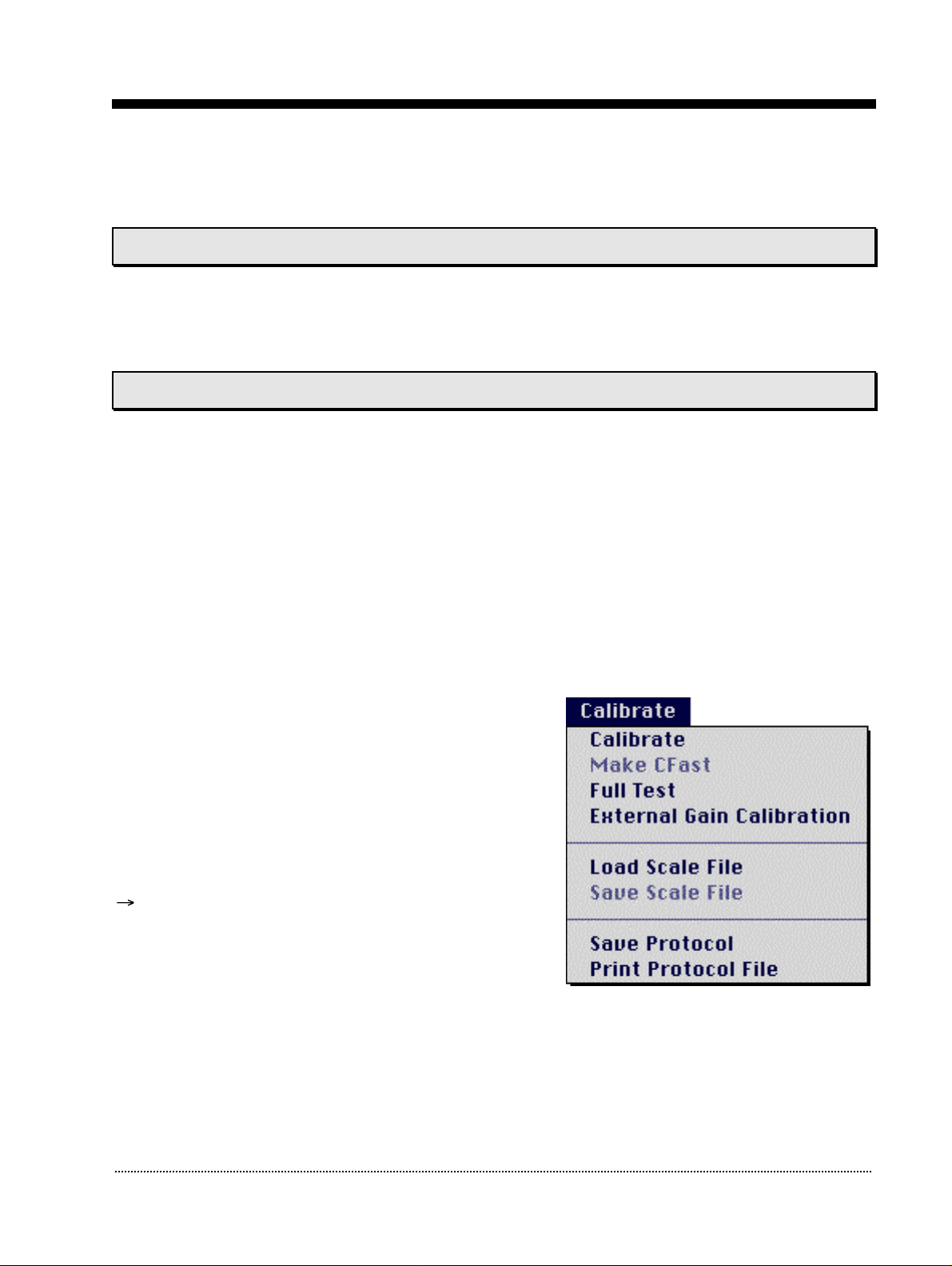
HEKA. In the program, go to the Calibrate

menu. This menu contains all the items involved in
calibration generation of scale files. If there is no
valid calibration, the menu item Make CFast will
be disabled. If you have an EPC9 Double or Triple
this menu item will also be disabled, unless each amplifier has been calibrated correctly.
To perform the calibration select Calibrate from the Calibrate menu. E9SCREEN will
warn you that this procedure may take up to 10 minutes, depending on the speed of
your computer (6 minutes on a 300 MHz PII system). Go ahead by clicking the Yes
button.

Installation EPC9 Installation 16

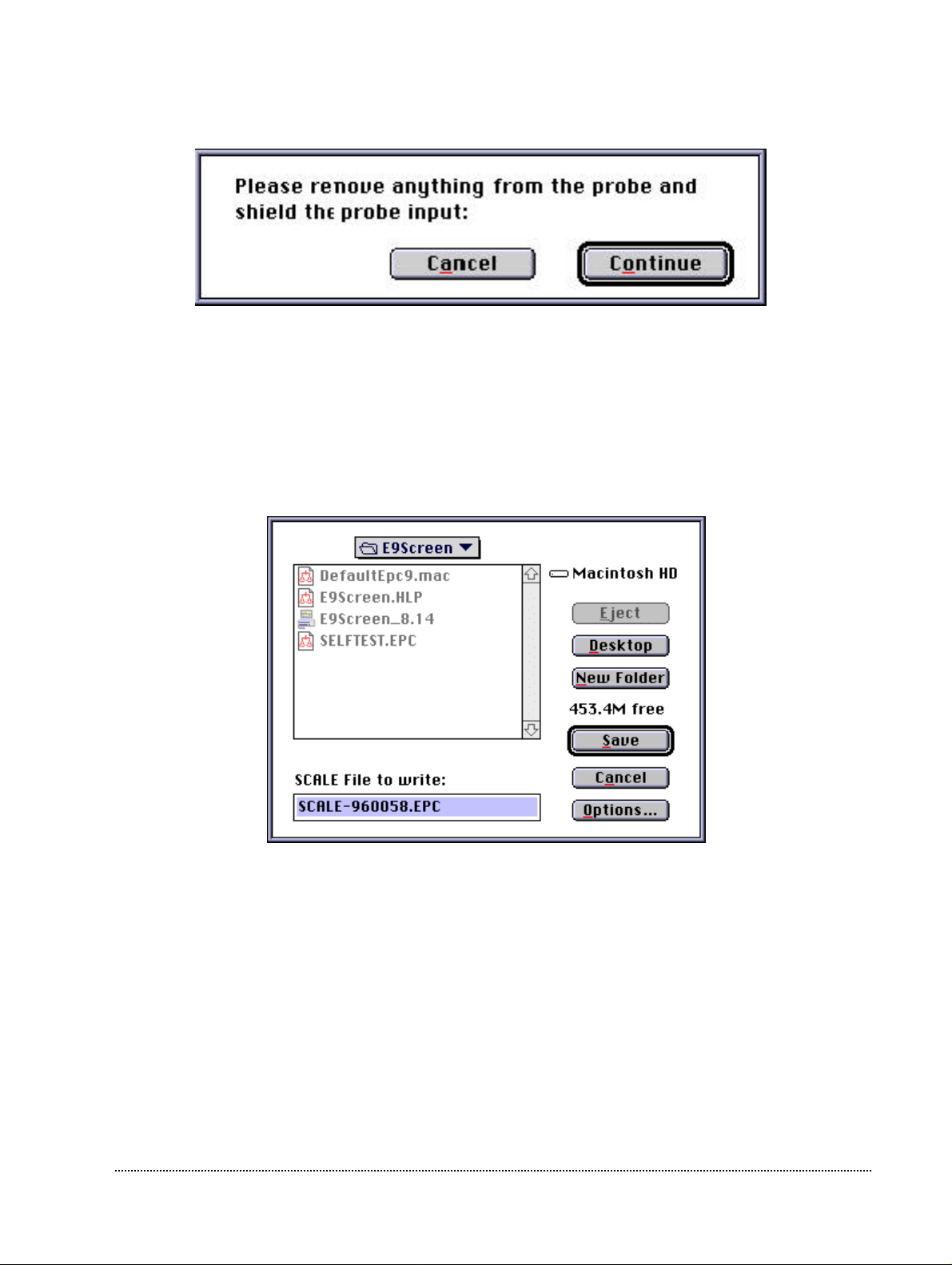
Then you are instructed to remove anything from the probe and shield its input:

You can use the metallic cap that came with your EPC9 and put it on the BNC connector
of the probe to shield it. Please make sure that really nothing except the metallic cap is
connected to the probe (the red and the black pin jack should be free) and that no BNC
cables are connected to the inputs and outputs of the EPC9 !

At the end of the calibration, E9SCREEN will let you know, whether the calibration
succeeded or failed. If it succeeded, the program will ask you, whether you want to save
the new calibration file and generates the proper name for the calibration file.

It is not advicable to save the file under a different name, because in that case you would
have to manually load the scale file during every initialization.

Note: It is very advisable to store the calibration files only in the one place. The best place to

put the calibration files is the E9Screen folder. Most users will run more than one
program which needs the calibration files to properly control the EPC9, e.g. PULSE and
E9SCREEN. Both programs will load by default the calibration files from the E9Screen
folder. If the calibration files are in multiple places the programs may load different
calibration files with possibly unpleasant consequences!

Finally, E9SCREEN re-initializes the amplifier.

Installation EPC9 Installation 17

If you have an EPC9 Double or Triple, you
should proceed to calibrate the second and
third amplifier as well. From the amplifier
pop-up menu, choose 2. Amplifier or 3.
Amplifier and repeat the steps listed above.

After having calibrated the amplifier (all amplifiers in case of an EPC9 Double or
Triple), you should also create a new C-fast lookup table for each amplifier as stated in
the next section.

Record

2. Amplifier Noise
WHOLE-CELLON-CELLSET-UP

Creating the C-fast Lookup Table

E9SCREEN and PULSE try to load the C-fast lookup table from the same location as the

calibration file when initializing the EPC9. You will get an appropriate error message, if
the Cfast file was not successfully loaded. To create a new C-fast lookup table select

Make CFast from the Calibrate menu in E9SCREEN. A confirmation dialog will be

displayed and will instruct you to remove anything from the probe and shield its input.
Again, please make sure that nothing is connected to the probe except for the metallic
cap that came with your amplifier. Now E9SCREEN will create the C-fast lookup table.
This usually takes a few minutes (30 seconds on a 300 MHz PII system). If you get the
message that the noise of the probe is suspiciously low this may indicate that your probe
is not connected to the main unit of the EPC9 – or you have a very good probe! Finally,
E9SCREEN will ask you to save the modified C-fast lookup table to disk and suggest a
reasonable path and file name corresponding to your active calibration.

Finally, E9SCREEN re-initializes the EPC9. If you have an EPC9 Double or Triple, you
should continue and create the C-fast lookup table of the second and third amplifier.
From the amplifier popup menu, choose ”2. Amplifier” or ”3. Amplifier” and repeat the
steps listed above.

Installation EPC9 Installation 18

4. Verifying and Testing the EPC 9

Testing the EPC9 with the Model Circuit

The following tutorial will guide you through most of the basic and some of the
unique and more sophisticated features of the EPC9 amplifier. At the same time it
allows you to check, whether the amplifier is functioning properly. You will use the
model circuit you got together with the amplifier as a substitute for a real patch­clamp recording and explore the virtual ”front panel” of the EPC9 supplied in the
program E9SCREEN.

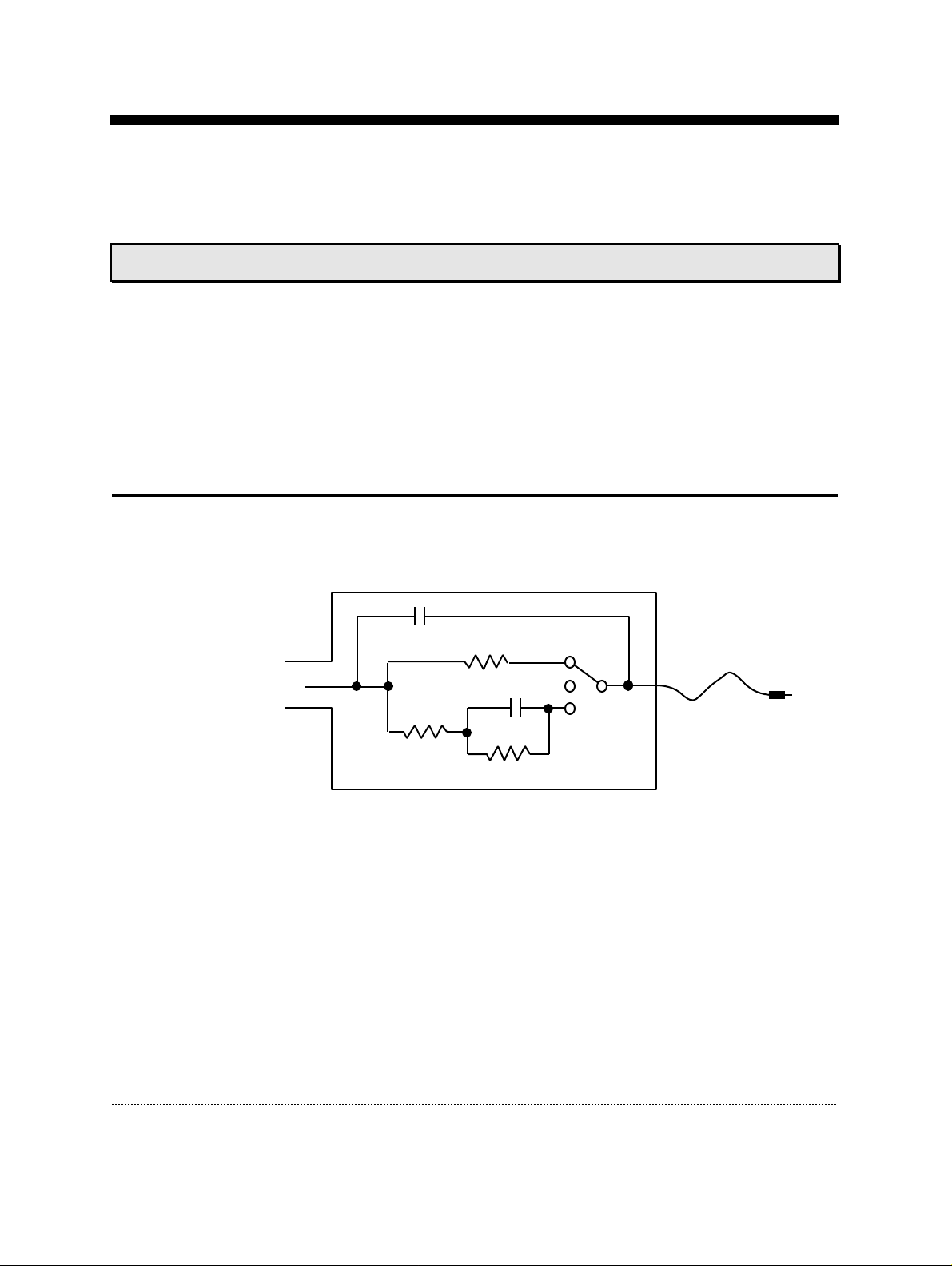
The Model Circuit MC 9

The model circuit connects to the probe input via a BNC adapter and the plug goes
to the black Gnd connector on the probe:

6 pF

BNC

(to probe

input)

5.1 MΩ

The model cell MC9

The model circuit provides a switch with three positions simulating the following
conditions typically observed during an electrophysiological experiment:

1. In the top position an ”open” pipette with a resistance of 10 MΩ is simulated.

This mode is useful for applying a test pulse and for correcting offset
potentials.

2. The middle position simulates a pipette attached to the cell membrane after

the Giga-Ohm seal formation. In this setting only a capacitance of 6pF is left
over corresponding to the ”fast” capacitance of a pipette sealed to the cell
membrane. This mode allows you to test the C-fast compensation.

10 MΩ

22 pF

Plug

(to GND

connector)

0.5 GΩ

Testing the EPC9 EPC9 Manual 19

3. In the bottom position a ”model cell” in the whole cell patch-clamp
configuration is simulated. The ”input resistance” is 5.1 MΩ, the ”membrane
resistance” is 500 MΩ and the ”membrane capacitance” is 22pF. This mode
lets you test the C-slow compensation and the current clamp mode.
Furthermore it is useful to check stimulation patterns you design within
PULSE.

Note: This model cell has a long “membrane” time constant (about 10 ms).

The following tutorial can be best executed with E9SCREEN. However, since PULSE
offers the same functionality with respect to the EPC9, you could use that program
instead. The figures shown were taken from E9SCREEN.

Step 1: Applying the Test Pulse

First, connect the model circuit to the probe input via a BNC adapter and plug the
black cable to the black ground connector on the probe. If E9SCREEN is not running
yet, start the program which is located in the E9SCREEN folder inside the HEKA folder.
Windows users might alternatively use the Start button to launch E9SCREEN from

Programs HEKA. The left side of the E9SCREEN window, the so called ”virtual front

panel”, provides a graphical representation of the EPC9 amplifier. The panel lets you
control all hardware settings of the amplifier(s) such as gain or filters. Signal display
is provided by an oscilloscope-like display in the right part of the window.

Testing the EPC9 EPC9 Manual 20

0.0 mV
Imon2

1. Amplifier

+/-

9

Vo -2.8 mV

Bessel 10 kHz

Record

8

LJ 0.0 mV

11

V-mon 0.0 mV

I-mon 3.53 pA

12

Filter 1
Filter 2 2.9 kHzBessel

EPC9 Patch-Clamp Amplifier, v8.3

Noise 0.00 A

WHOLE-CELLON-CELLSET-UP

Gain

5

5.0 mV/pA

Sound

Mode VC
Rmem 10.0 MΩ

Help

7

TrackAuto

emptyemptyemptyempty

ClipV-memb

Hz/MΩ Rmem

Sound

Volume

Last V-memb

2

6

Relative Value

CC Fast Speed

10

CC-range: 1pA/mV

Gentle CC-Switch: ON

100

100 %

1

Reset

CFast

Range Off Cap Track

CSlow

RSeries 5.0 MΩ

0.00 pF
50 %

1.00 pF

RsComp

0.5 µs

<>

Auto

Delay Off

<>

Auto

OffOff

500. pA

1.20 ms

Amplitude

Test Pulse

Duration

5.0 mV

5.0 ms

Stimulus External

Off20 µs

3

Scope

4

Off TrackAuto

Gain

OverlayClose

1.02 x

Leak Subtraction

Clear

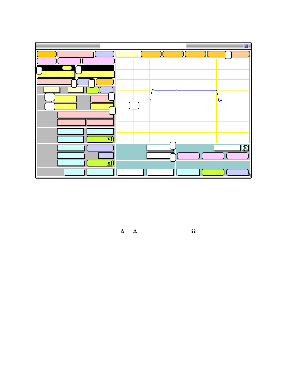
Put the model circuit into the ”10 MOhm” setting, which simulates a 10 MΩ-pipette
that is open to the bath solution. Reset the amplifier (1), set E9SCREEN to VC
(”voltage clamp”) mode (2) and apply a test pulse of 5 mV amplitude (3) and 5 ms
duration (4). The current response will be displayed on the digital oscilloscope. If
your gain range is appropriate, i.e. 5 mV/pA (5) you should a see a rectangular
current of about 500 pA in response to the test pulse. This represents the ohmic

resistor you are recording from: I = U / R = 5 mV / 10 M = 500 pA. E9SCREEN
will online calculate the pipette resistance and update it in the Rmem field (6) where

you should read a value close to 10 MΩ.
A possible voltage offset can be automatically canceled by clicking on the Auto-V0

button (7). After doing so, the command potential will be set to 0 mV (8) and the V0
control (9) displays the offset potential. The baseline of the current response (10), the
voltage monitor V-mon (11) and the current monitor I-mon (12) should be close to
zero. You could also do the offset potential cancellation in a more classical way by
clicking into the V0 control (9) and dragging the mouse up and down until the first
segment in the oscilloscope and the I-mon display (12) match zero.

The steps listed above can be automatically executed by clicking on the SET-UP
button or pressing the ‘1’ key on the numerical keypad. This will execute the

Testing the EPC9 EPC9 Manual 21

following built in macro that resets the amplifier, creates a rectangular test pulse, sets
the gain of the amplifier to 5 mV/pA and then performs an automatic compensation
of the voltage offsets:

1 : SET-UP
E Reset: ; reset the amplifier
E PulseAmp: 5.0mV ; set test pulse amplitude
E PulseDur: 5.0ms ; set test pulse duration
E Gain: 10 ; set gain to 5.0 mV/pA
E AutoZero: ; compensate voltage offsets
E SoundOn: TRUE ; beep
E SoundOn: FALSE ;

Note: E9SCREEN has a built in macro interpreter that executes command lines of the

form ”Window Control[: parameter; comment]”. E.g., the line ”E Gain: 10” would
instruct PULSE and E9SCREEN to set the gain popup in the EPC9 window to the

10th value (5 mV/pA). The predefined macros are stored in a text file called

”DefaultEpc9.mac” and can be edited with any text editor. For this tutorial it is not
necessary to know all possible commands and their syntax. Therefore, please, refer
to the PULSE manual for a detailed description on how to record and modify
macros.

Testing the EPC9 EPC9 Manual 22

Step 2: ”On-Cell” Voltage-Clamp Recording

Now move the switch of the model circuit to the center position which leaves only a
capacitance of about 6 pF connected. This simulates a Giga-Ohm seal and the C-fast
controls can be used to cancel the capacitive spikes resulting from the stimulus test
pulse.

EPC9 Patch-Clamp Amplifier, v8.3

Record

LJ 0.0 mV

V-mon 0.0 mV

I-mon -524. fA

1. Amplifier

+/-

0.0 mV
Imon2

Vo -2.5 mV

Noise 0.00 A

WHOLE-CELLON-CELLSET-UP

Gain

20 mV/pA

Sound

Mode VC
Rmem 94.3 GΩ

ClipV-memb

Help

TrackAuto

emptyemptyemptyempty

1

Before C-Fast compensation

After C-Fast compensation

Reset

Filter 1
Filter 2 2.9 kHzBessel

CFast

Range Off Cap Track

CSlow

RSeries 5.0 MΩ

RsComp

Bessel 10 kHz

2 3

6.23 pF
79 %

1.00 pF

8.0 µs
<>

Auto

4

Delay Off

<>

Auto

OffOff

128. pA

1.20 ms

5

Amplitude

Test Pulse

Duration

5.0 mV

5.0 ms

Stimulus External

Scope

Gain

OverlayClose

1.00 x
Clear

Leak Subtraction

Off20 µs

Off TrackAuto

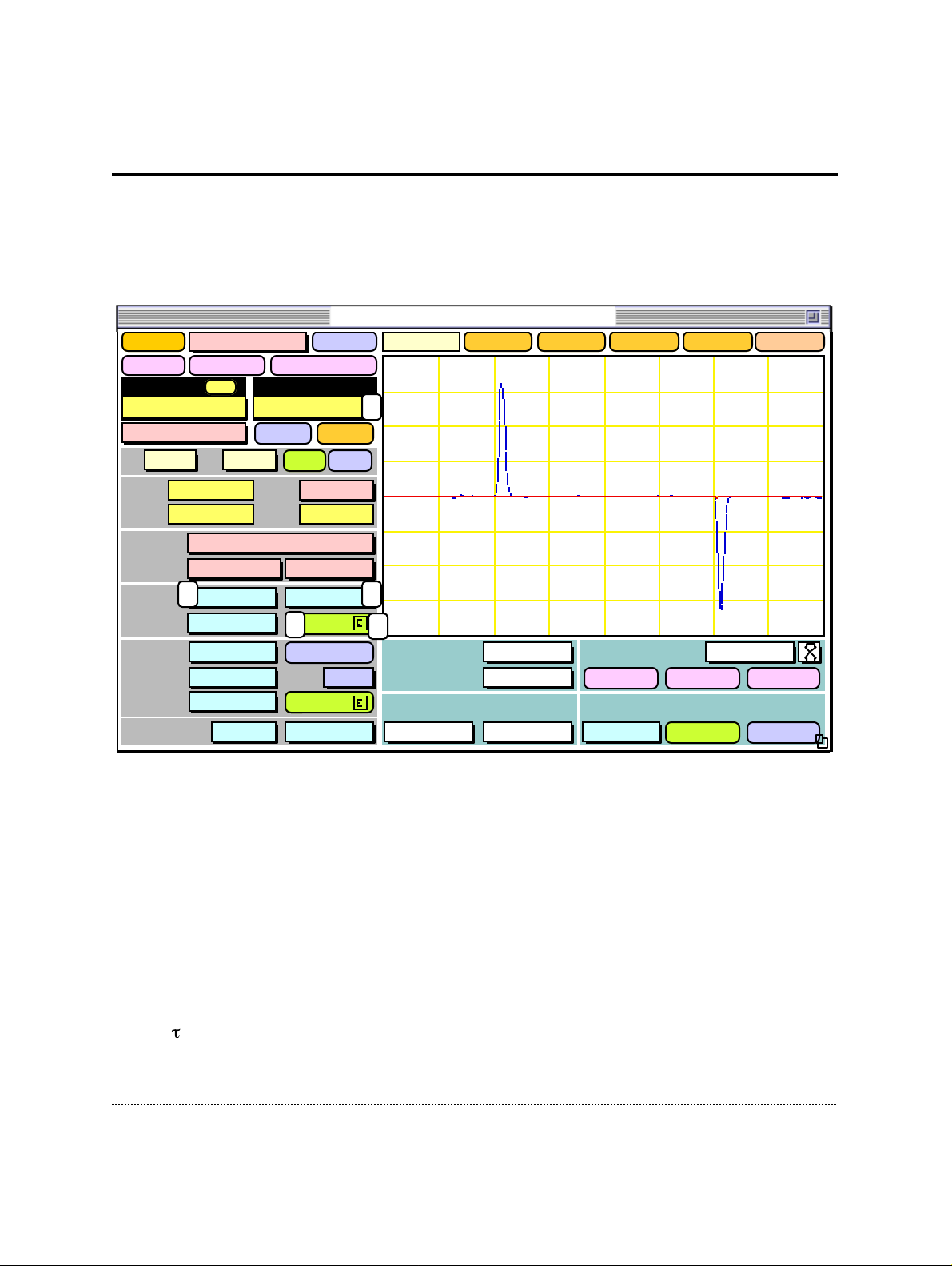
In order to see the small currents resulting from the high resistance of the model
circuit, set the gain to 50 mV/pA by either using the gain popup menu (1) or by
hitting 3 times the up arrow key.

Note: Alternatively to using the mouse, most of the controls can also be changed directly

by the keyboard. You can see the actual keyboard assignments, when you select

Show Keys from the Help menu.

In the oscilloscope you will see two fast capacitive transients (blue line) coming from
the 6 pF capacitor in the model circuit. Activate the C-fast compensation by clicking
into the C-fast field (2) and dragging the mouse upwards. While you are approaching
a value close to 6 pF you should see the spikes become smaller. You may have to

adjust -fast (3) in the same way. As soon as you are overcompensating you will see
the spikes going into the opposite direction. This indicates that you should decrease

Testing the EPC9 EPC9 Manual 23

C-fast – using the model circuit it is not very critical to misadjust -fast. Continue
adjusting C-fast and -fast unless you see an almost flat line in the oscilloscope (red

line). This should be the case at a around 6 pF (2).
Instead of compensating C-fast ”by hand” you can also press the Auto button (4) in

the CFast section of the amplifier control panel for an automatic compensation of C-
fast and -fast. If the compensation fails, the E-field (5) in the Auto button becomes

black. If this happens, you should repeat the auto-compensation, until it succeeds
and the E-field becomes normal again. The steps listed above can be automatically
executed by clicking on the ON-CELL button or pressing the ‘2’ key on the numerical
keypad. This will execute the following predefined macro that increases the gain and
then performs twice an auto-compensation – considering a possible failure in the
first attempt.

2 : ON-CELL
E Gain: 14 ; set gain to 50 mV/pA
E AutoCFast: ; automatic C-fast compensation
E AutoCFast: ; repeat compensation
E SoundOn: TRUE ; beep
E SoundOn: FALSE ;

Step 3: ”Whole-Cell” Voltage-Clamp Recording

After compensating C-fast well you can now switch into the “0.5 GOhm” position of
the model circuit. This will simulate a “model cell” with 22 pF ”membrane

capacitance”, 500 M Ω “membrane resistance” and 5.1 MΩ “input resistance” in the
whole-cell configuration. This mode can be used to verify the C-slow controls, the
action of series resistance compensation with C-slow enabled, and the current clamp
mode (see below).

After reducing the gain to 20 mV/pA (1), the Rmem field should reflect the changed
“membrane” resistance and display a value close to 500 MΩ (2). You should see in

the oscilloscope two capacitive transients (blue line) caused by the 22 pF capacitor in
the model circuit. The “slower” time constant of the model cell – compared to the

“fast” time constant from the middle position – is τ = Rs ⋅ Cm = 5.1 M Ω ⋅ 22pF = 112

µs. The peak current can be calculated from I

= Cm ⋅ U / = 22 pF ⋅ 5 mV / 112 µs

max

= 982 pA. With the actual gain setting of 20 mV/pA this would generate a voltage of

19.6 V at the current-to-voltage converter output, which exceeds the amplifier’s
voltage range. This is signalized by the red Clipping indicator at the amplifier and in
the ”virtual panel” in E9SCREEN (3).

Activate the C-slow compensation by selecting the 100-pF range from the Range field
(4). Now start the compensation by increasing the CSlow (5) and the RSeries (6)

Testing the EPC9 EPC9 Manual 24

values – again by clicking and dragging the mouse upwards. Since there are two
variables to adjust this is more difficult than the C-fast compensation. However, with
some praxis you will get a better feeling for these parameters and how they effect the
recording. With increasing quality of the compensation you should approach the real
values of the model circuit and the transients should disappear (red line). Instead of
compensating C-slow “by hand” you can also press the Auto button (7) in the CSlow
section of the amplifier control panel for an automatic compensation of C-slow and R-
series. If the compensation fails, the E-field (8) in the Auto button becomes black.
When this happens, you should repeat the auto-compensation, until it succeeds and
the E-field becomes normal again.

Note: The speed and success of automatic C-slow compensation depends on the actual

values of C-slow and R-series. These two values should be reasonably near to the
real values. Therefore, you should always check, whether the values are reasonable
before executing the automatic compensation. It is much better to have too large
estimates than too small ones.

Clicking the Cap Track button (9) does this automatic compensation repetitively after
a delay you specify in the Delay field (10). With a delay of 1 ms and a contemporary
computer (Pentium II, 300 MHz) this feature allows you to measure the membrane
capacitance at a rate of 15 Hz. You can output the results of the Cap-Track mode into
the notebook window, if you activate the option Log Tracking from the EPC9 menu.

Note: If you are a novice to patch-clamping it is useful to perform the C-fast and C-slow

compensation at least a couple of times manually before getting used too much to the
convenience of the automatic routines. Doing so you will get a better feeling for the
quality of a recording and how it is affected by the various parameters, especially the
input resistance R-series.

In a similar way as you explored the C-slow compensation, you could now have a
closer look into the Rs-Compensation. Turn the compensation on by setting an

appropriate compensation speed, 2, 10 or 100 µs (11), and gradually increase the
percentage of compensation from 0 to 95% by clicking and dragging the mouse
upwards (12). As soon as you are overcompensating the series resistance typical
oscillations will occur in the oscilloscope. Series Resistance Compensation is a more
complicated topic and is therefore treated in more detail in the EPC9 Manual.

The steps listed above can be automatically executed by clicking the WHOLE-CELL
button or pressing the ‘3’ key on the numerical keypad. This will execute the
following macro that sets the right gain, does a C-Slow compensation with
reasonable values:

Testing the EPC9 EPC9 Manual 25

3 : WHOLE-CELL
E Invert: TRUE ;
E Gain: 12 ; set gain to 20 mV/pA
E CSlow: 30.00pF ; set C-Slow value to 30 pF
E RSeries: 10.0MO ; set R-Series value to 10 MOhm
E AutoCSlow: ; automatic C-slow compensation
E AutoCSlow: ; repeat compensation
E SoundOn: TRUE ; beep
E SoundOn: FALSE ;

Step 4: ”Whole-Cell” Current-Clamp Recording

If C-Slow has been compensated so far, switch into the current-clamp mode by
selecting CC from the Mode popup (1). This should automatically select the voltage
monitor Vmon (2) to become your active channel displayed in the oscilloscope. If this
is not the case, e.g. with older versions of E9SCREEN or PULSE, change the active
channel to Vmon (2). Note, that the unit of the test pulse amplitude changes from
“mV” to “pA” as soon as you switch from voltage into current clamp mode (3).
E9SCREEN and PULSE use two different amplitudes for VC and CC modes,
therefore the test pulse is set to “0 pA” initially. Now you need to inject current into
the circuitry, 100 pA should be a reasonable value (3). The current injection will

charge the “membrane” of the “model cell” at a time constant = Rm Cm = 500 MΩ ⋅
22pF = 11 ms to a final value of V

slower time constant compared with voltage clamp conditions it takes much longer
to reach V

, therefore you should increase the duration of the test pulse to a more

max

appropriate value of 100 ms (4).

= Rm I = 500 MΩ ⋅ 100 pA = 50 mV. Due to the

max

Note: In contrast to voltage clamp conditions, were τ is proportional to the access- or series

resistance (Rs) of the pipette, in current clamp experiments τ depends on the
membrane resistance (Rm).

The normal setting of the oscilloscope scales the voltage monitor at 250 mV per
division. You should therefore increase the gain of the oscilloscope to 16 (5) which
scales the display to be 16 mV per division. Please remember that the oscilloscope
gain is different from the amplifier gain and only scales the display, not the
acquisition of data. Using a very high oscilloscope gain together with a low amplifier
gain allows you to determine the digital resolution of the analog-to-digital converter.

The EPC9 has two feedback circuitry for current clamp recordings. The so called
“fast” current clamp mode was introduced with the “C” version of the hardware in
1995 and is also available in the EPC8. The EPC7 and older EPC9 amplifiers (“A” and
“B” version) lack the fast current clamp mode. The board version of your EPC9
amplifier is displayed in the last menu item of the EPC9 menu. If your amplifier
supports the fast current clamp speed it will be activated by default (blue line in the
oscilloscope). To turn this mode off close the oscilloscope (6), click the red button

Testing the EPC9 EPC9 Manual 26

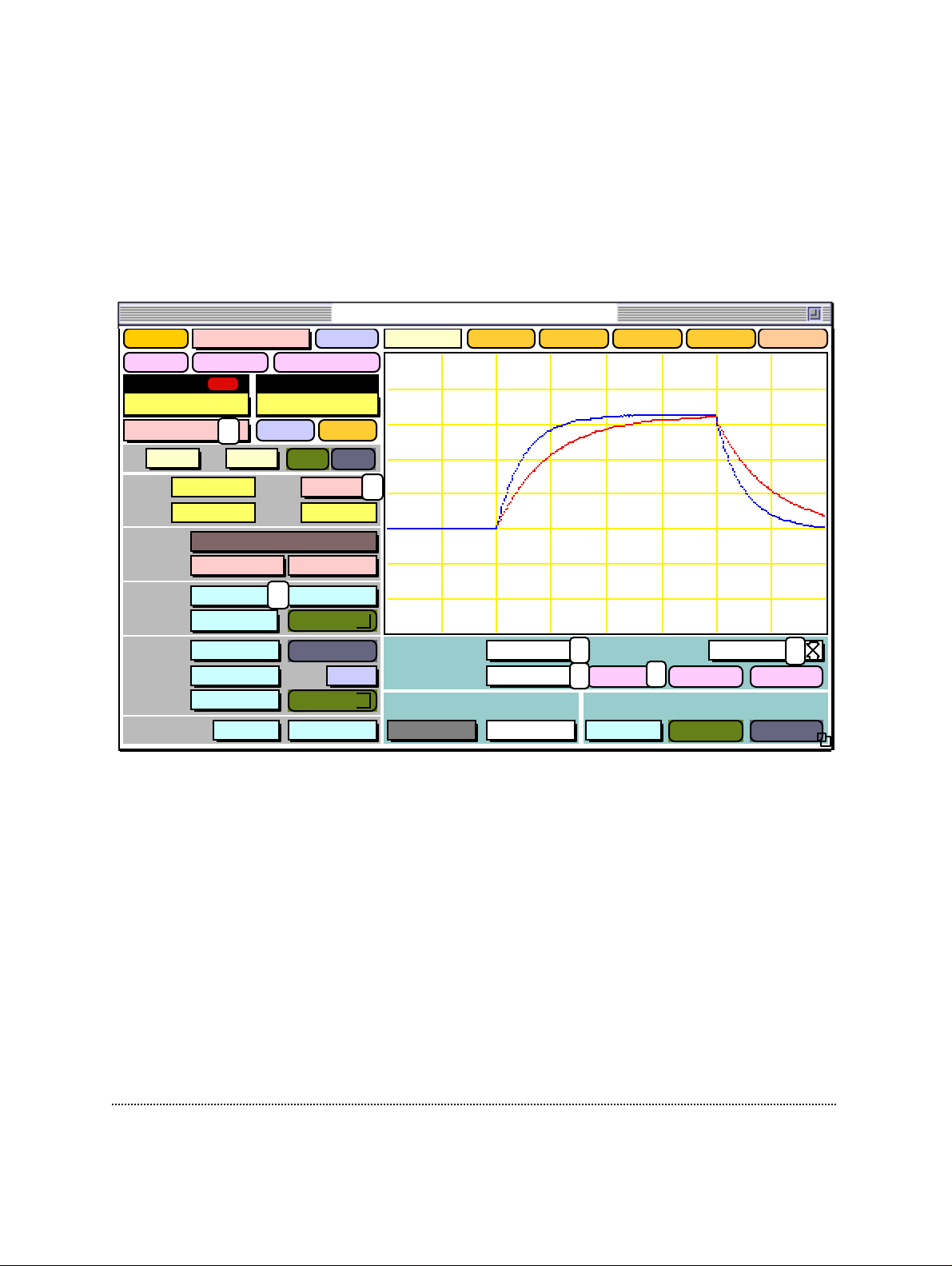
labeled CC Fast Speed and then open the oscilloscope again (6). Now, you will see a
much slower signal (red line in the oscilloscope). Please note, that the fast current
clamp mode is very sensitive to misadjustment of the C-fast setting. Especially
overcompensation causes the signal to oscillate. You can test this quickly by slightly
increasing C-fast from its value of about 6.5 pF (7). With the settings from this tutorial
you should see oscillations occur at a around 8.1 pF and above, when the fast current
clamp mode has been activated.

EPC9 Patch-Clamp Amplifier, v8.3

Record

-30.0 pA
Vmon

LJ 0.0 mV

1. Amplifier
WHOLE-CELLON-CELLSET-UP

+/-

10 mV/pA

Sound

2

Vo -2.2 mV

Noise 0.00 A

Gain

ClipI-hold

Help

TrackAuto

emptyemptyemptyempty

Fast Current-Clamp

Reset

V-mon -16.0 mV

I-mon -31.3 pA

Filter 1 Bessel 10 kHz
Filter 2 2.9 kHzBessel

6.50 pF

CFast

Range Off Cap Track

CSlow

RSeries 5.4 MΩ

21.71 pF

RsComp

Mode CC
Rmem 519. MΩ

67 %

8.0 µs

7

Auto

<>

Delay Off

<>

Auto

1

16.0 mV

25.0 ms

Amplitude

Test Pulse

Duration

Stimulus External

OffOff

Slow Current-Clamp

100.0 pA

100.0 ms

Off20 µs

Scope

3
4

Off TrackAuto

16.00 x

6

Gain

OverlayClose

Leak Subtraction

5

Clear

Note: The 500 MΩ setting of the model circuit is not a good method for testing the fast

clamp speed of the EPC9 due to the long time constant of 11 ms which the amplifier
can easily follow. If you want to have a better estimation of the amplifier’s speed
under current clamp conditions you should do the same test as above with the 10
MΩ setting. This results in a much shorter “membrane” time constant of only 60 µs.

Testing the EPC9 EPC9 Manual 27

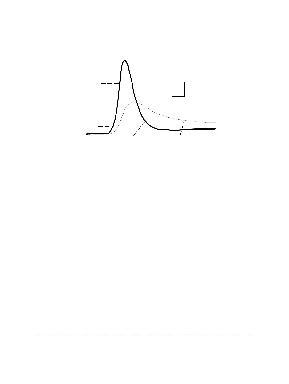
The following figure shows a recorded action potential (from H. Taschenberger & H.
von Germsdorff):

Presynaptic Action Potential

of the Calyx of Held

in the Rat Brainstem

0 mV

20 mV

250 µs

-60 mV

fast current clamp

normal current clamp

Testing the EPC9 EPC9 Manual 28

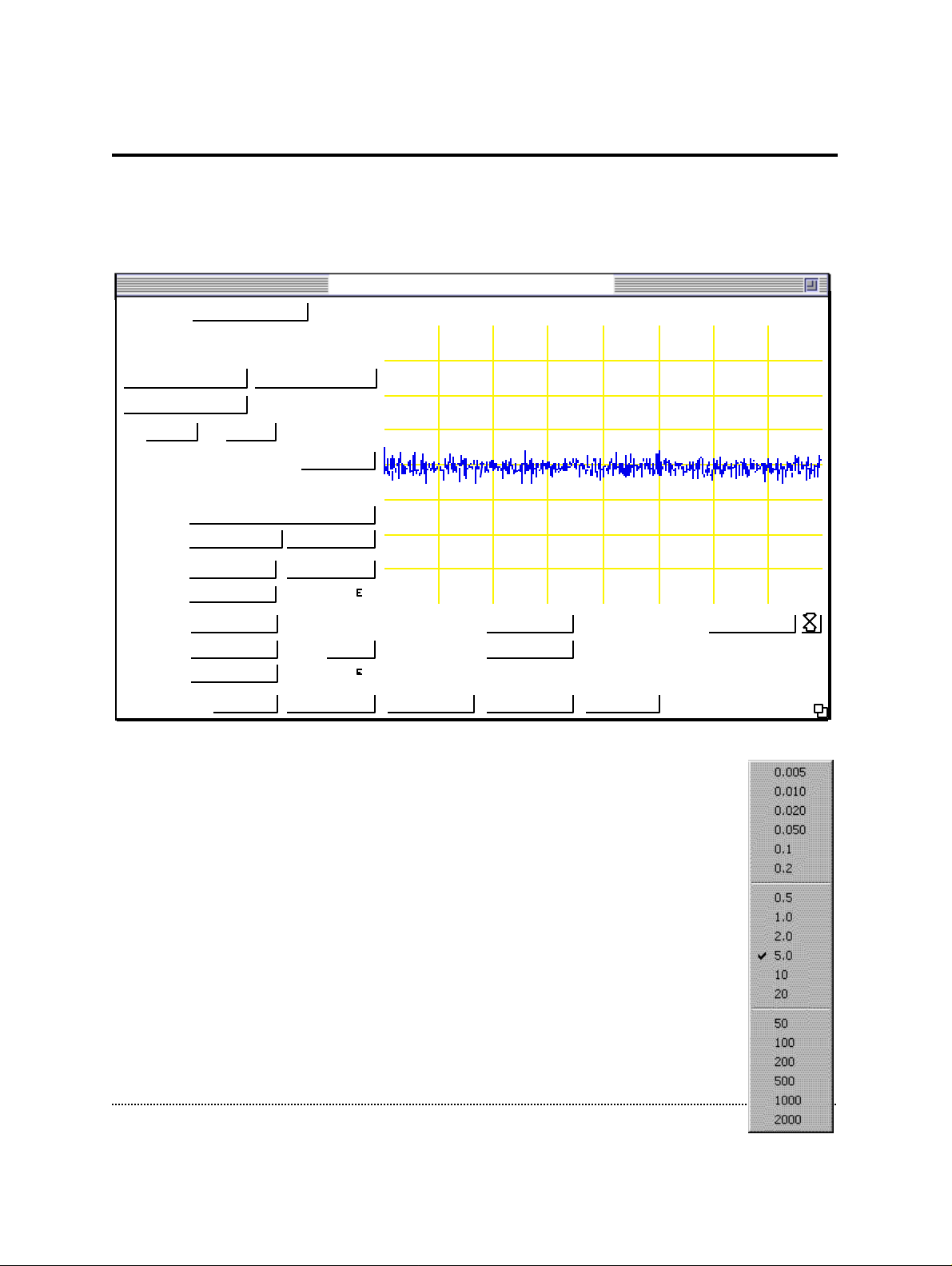
Step 5: Measuring the Noise of the Amplifier

Now let us come to the final section of the tutorial and check the intrinsic noise of the
amplifier. E9SCREEN has a built in feature that allows you to easily and quickly
check the noise of your amplifier and to minimize your setup’s noise, e.g., by
optimizing the grounding of the setup.

EPC9 Patch-Clamp Amplifier, v8.3

Record

0.0 mV
Imon2

1. Amplifier
WHOLE-CELLON-CELLSET-UP

+/-

50 mV/pA

Sound

Vo -2.7 mV TrackAutoLJ 0.0 mV

Noise 83.9 fA

1

Gain

ClipV-memb

3

Help

84.7 fA

2

emptyemptyemptyempty

Reset

V-mon 0.0 mV

I-mon -37.8 fA

Filter 1
Filter 2 2.9 kHzBessel

0.00 pF

CFast

Range Off Cap Track

CSlow

RSeries 5.0 MΩ

1.00 pF

RsComp

Mode VC
Rmem 41.4 MΩ

Bessel 10 kHz

8.0 µs

100 %

Auto

<>

Delay Off

<>

Auto

OffOff

4

512. fA

25.0 ms

Amplitude

Test Pulse

Duration

Stimulus External

100.0 ms

5.0 mV

Off20 µs

Scope

5

Off TrackAuto

Gain

100.00 x

OverlayClose

Leak Subtraction

6

Clear

First, remove anything from the probe and shield its input with the metallic cap.
Now click the Noise button (1) to start the noise test. In the noise-test
mode no stimulation will occur. Instead, E9SCREEN will calculate the
noise of the current monitor 2 (Imon2) and display it in (2). Select the
highest feedback resistor of the preamplifier, which has the lowest
intrinsic noise by switching into a gain of 50 mV/pA or higher (3).

Note: The three different gain ranges of the EPC9 are separated by lines in the

gain popup menu. The low-gain range goes from 0.005 to 0.2, the
medium-gain range from 0.5 to 20 and the high-gain range from 50 to
2000 mV/pA.

Note: Because of poor dielectric properties in the internal switch, the model

circuit introduces excess random noise above the level that can be
obtained with a gigaseal.

Testing the EPC9 EPC9 Manual 29

The action of the internal filters on the background noise level and the temporal
response can be observed by changing Filter 1 and Filter 2. An improved signal-to­noise ratio should be apparent when the Gain is increased to 50 mV/pA or greater
(which selects the 50 GΩ measuring resistor).

With filter 2 set to 2.9 kHz (4) and nothing attached to the probe you should read a
noise value between 90 and 110 fA (2).

Tip: If you wish to ground your setup you should now attach the pipette holder to the

probe, insert a glass pipette, bring the pipette tip into the recording position near the
recording chamber and power on every piece of equipment that introduces noise
(lamps, oscilloscope, camera, ...). Setting the duration of the test pulse to 100 ms (5)
and the gain of the E9SCREEN oscilloscope to a high value (6) will make the noise
and the 50/60 Hz pickup very obvious. In a well grounded setup all these
components should introduce no more than about 100 fA of additional noise.

Testing the EPC9 EPC9 Manual 30

Making a ”Full Test”

If you ever encounter any hardware problems that can not be solved by simply re­calibrating the amplifier (see Calibrating the EPC 9 on page 16) you can run the Full
Test in E9SCREEN. This feature is a diagnostic tool that allows us at HEKA
Elektronik to make some conclusions about possible defects of the amplifier.
Otherwise, this function and its output should only be of little interest for you.

Note: The Full Test sometimes reports errors although the amplifier is absolutely fine. This

may have multiple reasons. First, we opted to have stringent test specifications such
that possible problems are not missed. Second, errors may be caused by procedural
errors, or even because of defective BNC cables. If you get the message that your
hardware might be “not ok”, please contact HEKA first and supply us the report
before sending the amplifier in. You might save yourself valuable time!

Before starting the Full Test you should make sure to have nearby a shield for the
probe (e.g., the metallic cap delivered with the EPC9), a 10 MΩ resistor (e.g., the

model circuit) and 5 short BNC cables. Start
the E9SCREEN program. In case you have an
EPC9 Double or Triple, select the amplifier
you want to test from the amplifier popup: 1.
Amplifier, 2. Amplifier or 3. Amplifier.

Record

2. Amplifier Noise
WHOLE-CELLON-CELLSET-UP

Now select the menu item Full Test from the Calibrate menu. You will be told to
remove everything from the probe and shield its input. You can use the metallic cap
that came with your amplifier and put it on the BNC connector at the probe to shield
it. Please make sure that really nothing except the metallic cap is connected to the
probe and that especially the red and the black pin jacks are free. You should also
make sure that no BNC cables are connected to the main unit of the amplifier.

After a short while you will be prompted to connect 3-5 BNC cables, depending on
the amplifier you are testing, see table below. The following figure shows you how
to make the connections for the EPC9. Please note, that the description of the analog­to-digital converter part (top row of BNCs) is for the EPC9 Triple and looks different
for the EPC9 and the EPC9 Double. The DA- and AD-channels are numbered from 0
to 3, and 0 to 7, respectively.

Testing the EPC9 EPC9 Manual 31

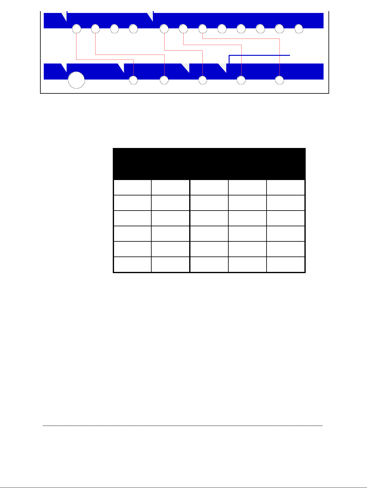
The following table shows you the combinations for the different amplifiers: EPC9,

EPC9

EPC9 Double

1. Amplifier

EPC9 Double

2. Amplifier

EPC9 Triple

1. Amplifier

EPC9 Triple

2. Amplifier

EPC9 Triple

3. Amplifier

0 0 11 22 3 3 54 6 7

PROBE

TEST

INPUT

EXTERNAL

STIM.INPUT

VOLTAGE
MONITOR

FILTER 1 FILTER 2

STIM1 STIM2 STIM3 TEST

IMON1 IMON2 IMON3 MUXVMON1 VMON2 VMON3

CURRENT MONITOR

EPC9 Double, and Triple. The EPC9 Triple has only one free AD input left (ADC-6),
the remaing channels are internally connected with the corresponding channels of
the amplifier. Therefore, only three connections (2 DA-channels and 1 AD-channel)
have to be made for the three amplifiers.

Amplifier Input Amplifier Output

Test Input External

Stim. Input

DAC 0 DAC 1 ADC 0 ADC 1 ADC 2

DAC 2 DAC 3 ADC 4 ADC 5 ADC 6

DAC 2 DAC 3 ADC 4 ADC 5 ADC 6

DAC 2 DAC 3 not tested not tested ADC 6

DAC 2 DAC 3 not tested not tested ADC 6

DAC 1 DAC 3 not tested not tested ADC 6

Voltage

Monitor

Filter 1 Filter 2

If the connection test fails, you will get an error message and the chance to repeat the
test an additional time. After the connection test you will have to remove all BNC

cables and connect a 10 MΩ resistor to the probe input. You can use the model circuit
and switch it into the “10 M” position. If the resistance is out of range (e.g. due to a
wrong position of the switch) you will see an error message and will be asked to
repeat the resistor test. After removing all BNC cables, you can proceed with the test.
It will continue for a while and you will get a final message reporting the status of
the amplifier, the probe and the connections. If any one of these fails you will see an
alert similar to the following one and get the chance to print out the error protocol.

Testing the EPC9 EPC9 Manual 32

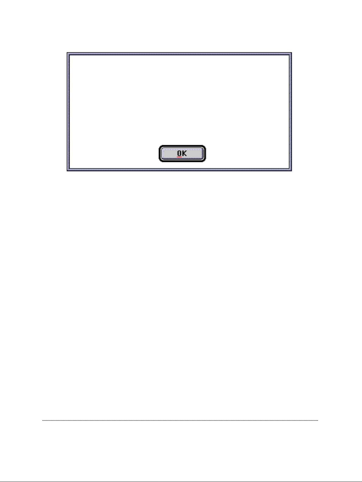
Status of EPC9:
Amplifier: OK
Probe: NOT ok
Connections: OK
Please, print now the protocol file, then conntact
HEKA or your EPC9 representative.
HEKA - Tel: [phone]

- Fax: [phone]

Important note:

Please, remind: if you get a message like this, please, contact HEKA first and
supply us the error protocol before sending the amplifier in. You might save
yourself valuable time and effort!

Testing the EPC9 EPC9 Manual 33

Measuring the Frequency Response

The Test mode allows one to easily check the basic current-measuring circuitry of the
EPC9. Select Test from the Mode list, connect a function generator or stimulator to
Test Input, and connect the right-hand Current Monitor Output (Filter 2) to an
oscilloscope. Alternatively, you can connect the Test Output of the internal
stimulator (DA 2) to the Test Input and look at the response. With the Gain set to 10
mV/pA, any signal applied to the Test Input connector should be reproduced with
the same amplitude at the Current Monitor Output. An applied signal amplitude of
about 1 volt is appropriate.

Note: The probe input usually needs to be shielded from low-frequency noise. A simple

way to do this is to cover the input connector with a cap made from aluminum foil.

Note: The Test mode current-injection system is intrinsically AC-coupled, which means

that long (>30 ms) pulses may be distorted in shape. Also, large low-frequency
inputs can cause the current-injection circuitry to saturate.

The action of the internal filters on the background noise level and the temporal
response can be observed by changing Filter 1 and Filter 2. An improved signal-to­noise ratio should be apparent when the Gain is increased to 50 mV/pA or greater
(which selects the 50 GΩ measuring resistor). If the signal source is a sine-wave
generator, the frequency response of the patch clamp can be verified directly.

Testing the EPC9 EPC9 Manual 34

5. E9SCREEN Software

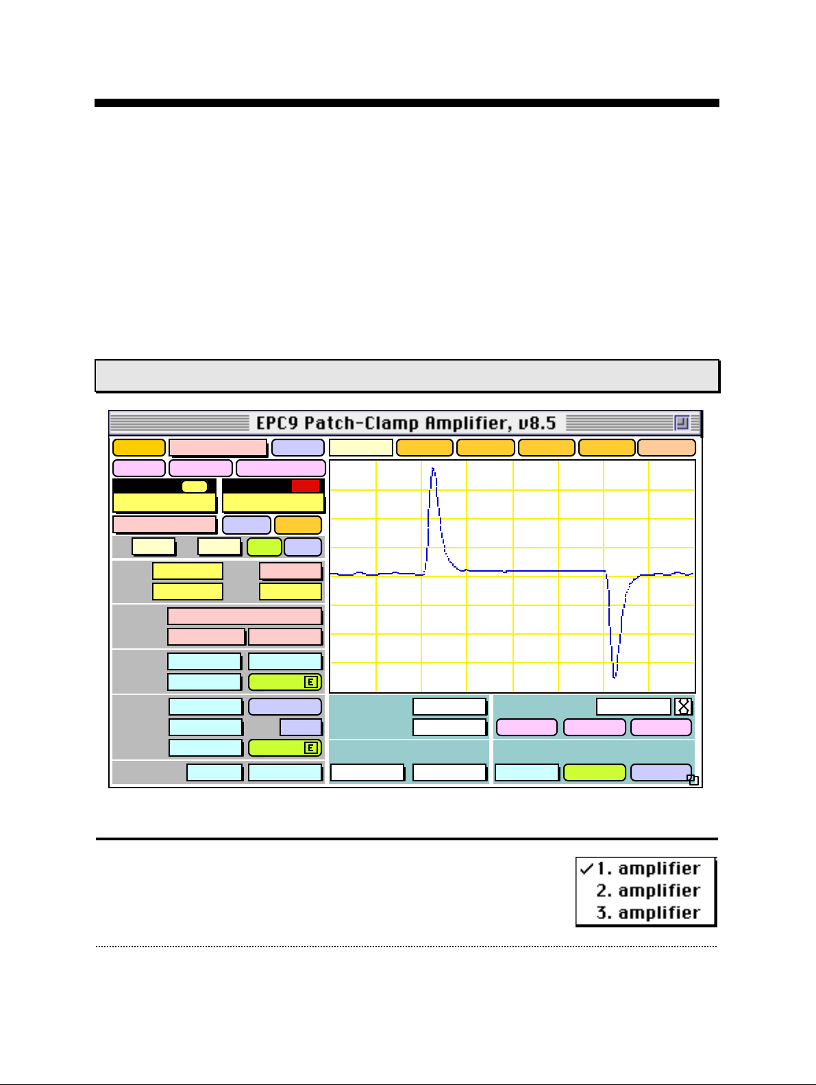
The E9Screen software provides the control and the graphical representation of the
EPC9 amplifier by a “virtual panel” with “buttons”. Signal display is provided by an
oscilloscope-like display. In addition, there is a Notebook window and drop-down
menus with options for the calibration procedures. E9Screen is mostly of interest to
those who use the EPC9 without Pulse, as it provides the only other means by which
the amplifier can be controlled. Pulse users will use E9Screen mainly for diagnostic or
calibration purposes.

EPC9 Window

ON-CELL

0.0 mV
Imon2

0.2 mV

12.2 pA

6.51 pF

1.00 pF

5.0 MΩ

1. Amplifier

+/-

-3.7 mV

Vo

Bessel 10 kHz

Bessel

65 %

Off

Off

Record

SET-UP

V-memb

LJ

0.0 mV

V-mon

I-mon

Filter 1
Filter 2

CFast

Range

CSlow

RSeries

RsComp

Main Controls

WHOLE-CELL

Gain

20 mV/pA

Sound

Auto

Mode
Rmem

535. MΩ

2.9 kHz

8.0 µs
Auto

<>

Cap Track

Delay

<>

Auto

Off

Noise

Clip

Help

Track

VC

Off

0.00 A

Hz/MΩ Rmem

Sound

CC-range: 1pA/mV

Gentle CC-Switch: ON

125. pA

1.00 ms

Test Pulse

Stimulus

20 µs

empty

Volume

Last V-memb

Relative Value

CC Fast Speed

Amplitude

Duration

6.0 mV

4.0 ms

External

100

100 %

Off

empty

Scope

Close

Gain

Overlay

Leak Subtraction

Off

emptyempty

Auto

Reset

1.02 x
Clear

Track

Amplifier Selection: On an EPC9 Double or Triple, one selects
the "active" amplifier from the "amplifier" pop-up list. Only the
available amplifiers can be selected in the amplifier list. When

E9Screen Software EPC9 Manual 35

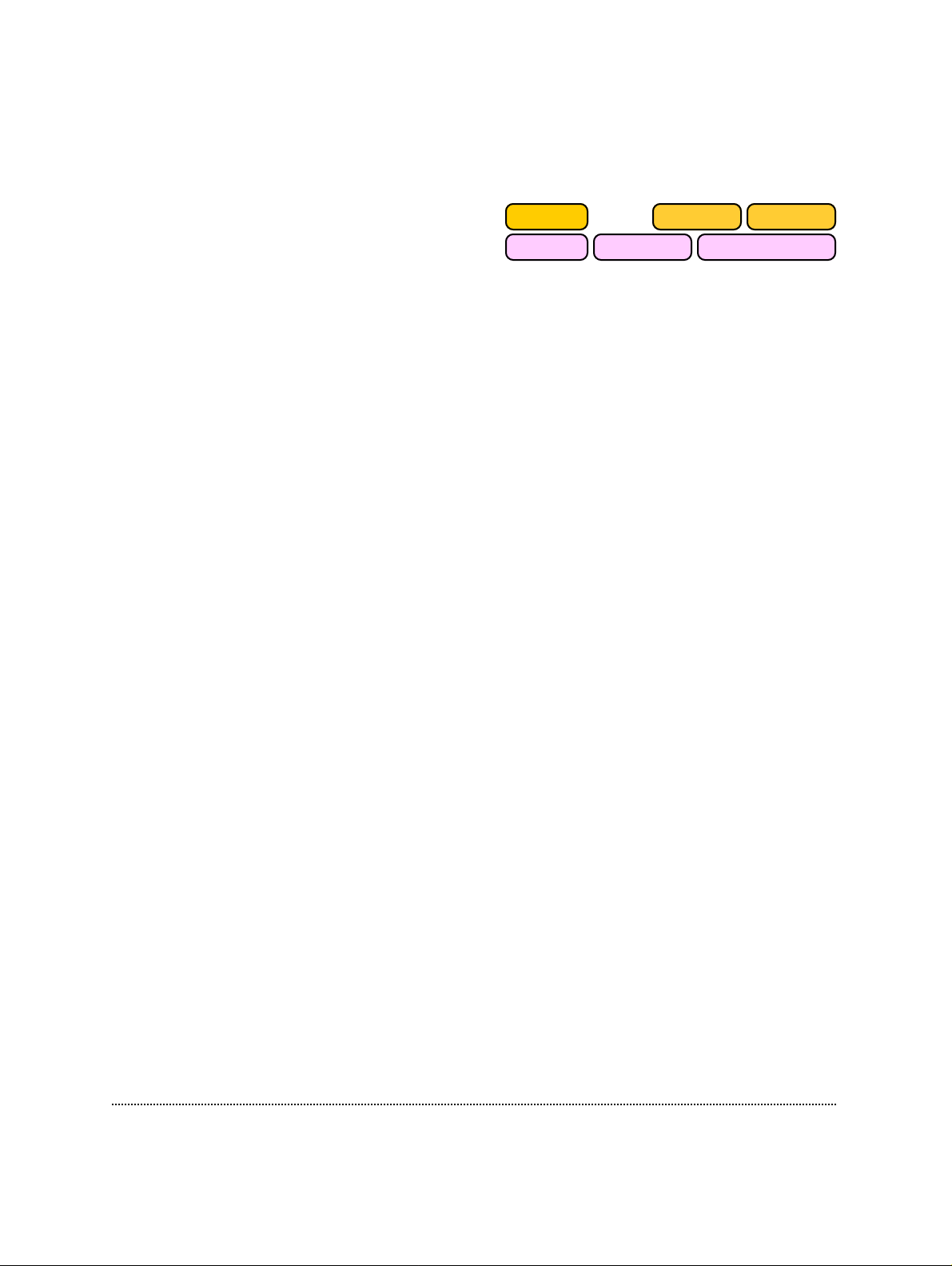
switching, E9Screen updates all parameters to show the state of the selected
amplifier. The state of each amplifier is independent of the settings of the other
amplifiers.

Macros: Macro buttons allow to record and

Record

emptyempty

play back a sequence of actions, such as
activation of buttons and parameter inputs

WHOLE-CELLON-CELLSET-UP

via mouse or keyboard. The macros Set-Up, On-Cell, and Whole-Cell are preset. Set-Up
resets all parameters (with the exception of LJ and V0), and defines the parameters of
the test pulse. On-Cell switches the Gain range to a typical setting for a cell-attached
patch recording, sets initial C-fast estimates, and invokes an Auto C-fast
compensation. Whole-Cell switches the Gain range to a typical setting for a whole-cell
recording, sets initial C-slow estimates, and invokes an Auto C-slow compensation.
These macros can be redefined and other macros be recorded using the macro record
function (see below). All macro controls that have nothing stored and therefore
perform no action are shown in white letters.

Note: The content of the macros can be written to the Notebook using the option

Macros…List in the EPC9 drop-down menu.

Record: To start macro recording, click on the Record button. Then, perform all
desired actions (the Notebook window will print a protocol of the macro actions).
While recording a macro you have the option of actually executing all actions as they
are entered or disable execution and only log the actions to the macro (see EPC9
menu Macro options). To specify a parameter value, enter it as usual by dragging or
typing. When clicking on a macro-button during recording, you will see a dialog
with the following options:

• Cancel: This will disregard the macro call. You can continue recording.

• Record call to macro itself: This will execute the macro as part of the macro

being recorded (embedded macro call).

• Copy contents of macro: This will copy each of the macro instructions of the

selected macro into the macro being recorded. This avoids the potential
problems of recursive macros (i.e., macros calling each other and causing an
infinite loop).

• Assign and name recorded macro: This will prompt you to give a name to the

macro. This name will become the button text.

Do not forget to save the macros in a file on disk (you can only save all 7 macros at
once). Otherwise they will only be remembered until you leave the program. The
default macro file is named “Default.Epc9_Macros” and it will be automatically
loaded next time the program is started.

E9Screen Software EPC9 Manual 36

Note: There is a limit of 50 actions per macro. To abort recording of a macro, click again

on “Record” and the just recorded sequence will be lost.

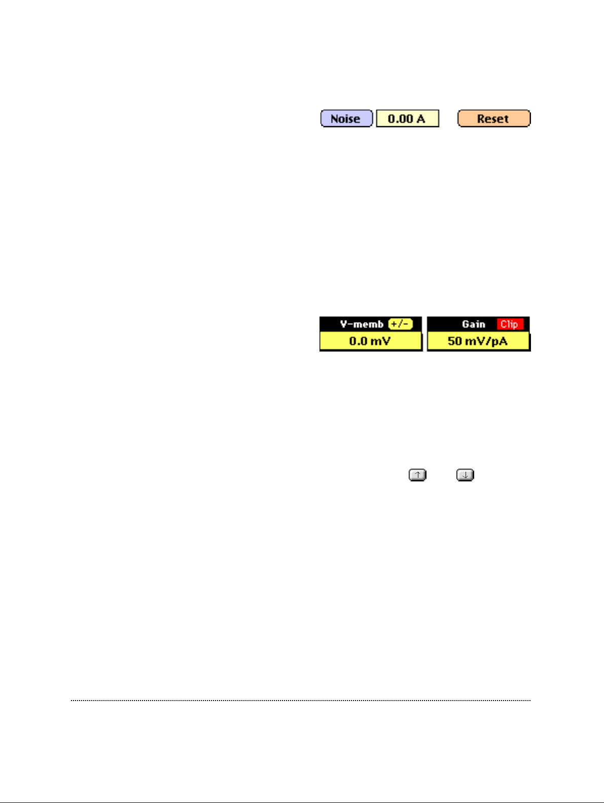
Noise: The rms noise is continuously
measured and updated when the noise
mode is selected with the button Noise. For the determination of the noise level, no
pulses are output and current is sampled via the active AD-channel using the current
filter settings (usually the Current Monitor 2 output, so that the bandwidth is
determined by Filter 2). It is sampled in sections of 10 times 256 points with a sample
interval of 100 µs, i.e., a total length of 256 ms.

I-monitor: DC current monitor.
Reset: Selecting this button will reset the EPC9 to its initial default configuration. It

will reset the DA channels to zero, which is useful to cancel the output of C-slow and
R-series set by Cap. Track. Also, Reset is very useful to define the initial state of the

EPC9, when recording a macro.
V-membrane: Displays the actually-

measured pipette voltage after correcting
for liquid-junction potentials and offsets
(provided the zero-current potential has been set correctly). This may differ
(temporarily) from the holding voltage (e.g., during long stimulation pulses) as it
indicates the average sum of V-membrane and the scaled stimulus voltage. V-
membrane is converted to I-hold in Current Clamp mode.

+/-: This button inverts the polarity of V-membrane.
Gain: Sets the scaling of the current monitor output. The range is 0.005 to 2000

mV/pA and can be set by dragging the mouse or pressing and . The gain
setting automatically selects one of the three available current-measuring feedback
resistors in the probe (5 MΩ, 500 MΩ, and 5 GΩ), corresponding to low, medium and
high gain ranges. The table below summarizes the main features and limitations of
the gain ranges:

E9Screen Software EPC9 Manual 37

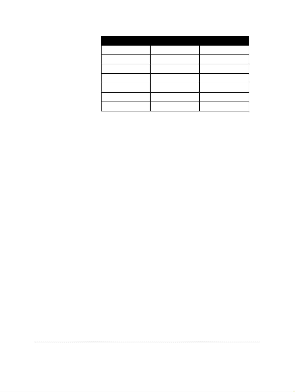
Low Medium High

Feedback Resistor 5 MΩ 500 MΩ 50 GΩ

Gain 0.005-0.002 0.5-20 50-2000

I

max

Bandwidth 100 kHz 100 kHz 60 kHz

C-slow Ranges 30 • 100 • 1000 30 • 100 • 1000 30 • 100

Current Clamp no yes no

Rs-compensation yes yes yes

± 2 µA ± 20 nA ± 200 pA

The lowest range may be used for experiments (e.g., bilayers, loose-patch, or large
cells) in which large currents need to be delivered (up to about 2 µA). Capacitance
compensation of up to 1 nF is available and Rs-compensation can be used for R

values down to 10 Ω in this range.
The medium and high gain ranges operate similarly to the EPC7. In the medium gain

range, the background noise is larger than in the high gain, but the full 100 kHz
bandwidth is available, and currents of up to about 20 nA can be recorded. This
range is used mainly for whole-cell recordings, and for this purpose the special
features of the 1000 pF transient cancellation range (see C-slow Ranges), series
resistance compensation, and the current-clamp modes are made available. On the
other hand, the high gain range is intended for single-channel recording. It has a
very low noise level, but this is obtained at the expense of a maximum current limit
of about 200 pA. The maximum available bandwidth is about 60 kHz, and the special
features mentioned above do not function in this range.

s

Slow capacitance cancellation ranges (30-100-1000 pF) can be set to any desired
value. However, in the high gain range (50 GΩ resistor) the 1000 pF range will not
operate. If the 1000 pF range is selected while the gain is higher than 20 mV/pA, the
gain will automatically be reduced to the highest possible setting (20 mV/pA).
Similarly, since the current-clamp mode is only possible in the intermediate gain
range (0.5-20 mV/pA), the gain will be reduced or increased appropriately when
selecting Current Clamp mode from an invalid gain range.

Clipping: A blinking box labeled “Clip” in the Gain title indicates saturation of
amplifiers in the current monitor circuitry. Like the Clipping LED on the EPC9 main
unit, this is a warning that excess artifacts or noise may occur due to the saturation of
amplifiers.

Note: This indicator may appear to be more sensitive than the LED on the EPC9. It is not;

it just latches the clipping status longer than the LED light.

E9Screen Software EPC9 Manual 38

AD-Channel: The oscilloscope can display the following:

• F2-Ext - External Stim. Input filtered by Filter 2

• Imon-1 - Current monitor 1

• Imon-2 - Current monitor 2

• Vmon - Voltage monitor output

• AD 0…5 - Any of the other AD channels.

The F2-Ext setting allows you to use Filter 2 as a general-purpose variable filter. In
this setting the External Stim Input becomes the filter input, and the filter output is
available at Filter 2 and is displayed in the Oscilloscope window.

Help: Displays keyboard equivalents that are assigned to EPC9 controls.
In this mode you can click on any control to have the Help window
display a short description of that control.

Sound: If this control is On, a sound is played with
its frequency coding for R-membrane. The sensitivity
(Hz/MΩ) and the volume can be specified. The
controls that set these parameters are normally
hidden, but may be accessed by closing the
Oscilloscope window.

V0 (Pipette Offset): V0 displays the offset

voltage (a voltage which is added to V­membrane to obtain the pipette command voltage). It can be set either by the Auto-V

operation or by manually dragging the mouse after clicking into the item.
Furthermore, V0 is changed automatically by the controlling program whenever the
user changes the variable LJ. This is necessary for LJ and the Auto-V0 operation to
interact properly. It is not recommended that the user changes V0 manually, because
this interferes with the software features for automatic offset correction.

Auto-V0: The Auto-V0 button calls a procedure for automatic zeroing of the pipette

current. Thereby, an offset voltage (V0) to the pipette potential is systematically
varied until pipette current is zero. Range of V0 is ± 200mV. Auto-V0 is typically
performed before seal formation. It works properly only when a pipette is inserted
into the bath.

The Auto-V0 procedure interacts with the variable LJ to provide for online correction
of liquid junction potentials and other offsets (see Chapter 7. Compensation

Procedures on page 59). This requires that V-membrane is set to the value of LJ (for On
Cell and In Out Recording Modes) or to the opposite polarity of LJ (for Whole Cell and

0

E9Screen Software EPC9 Manual 39

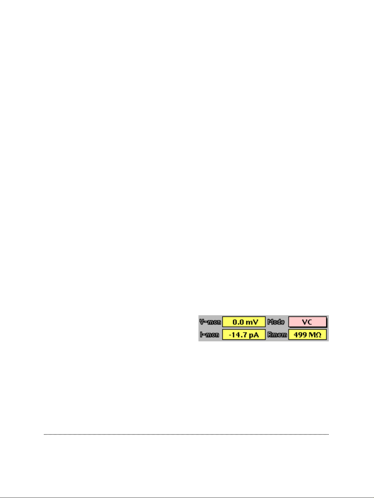
Out Out Recording Modes), before the actual zeroing operation is performed. Auto-V
does this automatically and leaves V-membrane at that value.

Note: V0 is not changed by the Reset function.
Track: This option implements a Search Mode (see Chapter 6. Operating Modes on

page 58), which is essentially a repetitive Auto-V0 procedure at a holding potential of

0 mV. The rate at which Auto-V0 is performed is determined by the Search Mode Delay
in the EPC9 menu.

LJ (Liquid Junction): LJ is a variable, to be set by the user, which allows to correct for
liquid junction potentials and other offsets. It works in conjunction with the V
operation. An online correction requires an Auto-V0 operation to be performed before
seal formation and LJ to be set to an appropriate value. No correction is performed if
LJ = 0. See Chapter 7. Compensation Procedures on page 59 for more information on
how to determine LJ.

LJ can be adjusted within ± 200 mV by dragging the mouse or typing after a double­click. Please note that LJ is not changed by the Reset function, and cannot be set by
macros. This restriction is imposed to avoid unintentional offset corrections.

LJ should be 0 mV when using identical pipette and bath solutions. It may be
changed to any desired value within ± 200 mV in case asymmetrical solutions are
used or the bath solution is changed during an experiment. For the standard liquid
junction potential correction, the polarity of the entered value should be such that it
represents the potential of the bath with respect to the pipette solution. For example,
if the pipette solution contains glutamate or aspartate (with chloride in the bath),
then the polarity of LJ should be positive (+10 mV). After an Auto-V0 operation, V-
membrane will be changed to -10 mV (in Whole Cell and Out Out Recording Modes) or
+10 mV (for On Cell and In Out Recording Modes), which corresponds to the true
zero-current potential.

0

0

V-mon: Displays the actually-measured
pipette voltage after correcting for liquid­junction potentials and offsets (provided the
zero-current potential has been set correctly). This may differ (temporarily) from the
holding voltage (e.g., during long stimulation pulses) as it indicates the average sum
of V-membrane and the scaled stimulus voltage.

I-mon: DC current monitor.
R-membrane: The Seal Resistance (R-membrane) is determined from the current

sampled during the baseline and the second half of the test pulse. R-membrane can be
encoded into a tone using the Sound feature.

E9Screen Software EPC9 Manual 40

Mode: Sets the Recording Mode (in the above example it is Voltage Clamp). For details
on the various recording modes see Chapter 6. Operating Modes on page 54.

• Test - Sets the Test mode.

• VC - Sets the Voltage Clamp mode.

• CC - Sets the Current Clamp mode.

When switching from voltage-clamp to current-clamp mode, I-hold will be set to
inject the holding current required to keep the membrane voltage constant (“gentle
switch”, see description of the Gentle CC-Switch control below, subchapter Hidden
Controls). Thus, V-mon will be identical to the original V-membrane commanded
under voltage clamp. In analogy, upon returning to voltage clamp, V-membrane will
be set according to the membrane potential under current clamp and rounded to the
next 2 mV.

Quite often, the membrane potential under current clamp will
have changed, and when returning to voltage clamp, V-

membrane will possibly differ from that set before switching to current-clamp mode.
Last V-membrane can then be used to conveniently restore the original V-membrane

value. This button is normally hidden behind the oscilloscope window; it can be seen
when closing the oscilloscope. For details see Chapter 6. Operating Modes on page 54.

Starting with the version “C” of the EPC9, the current-clamp
circuitry has two speed settings (which can be toggled by a
button that is normally hidden behind the oscilloscope window; it can be seen when
closing the oscilloscope). For details see Chapter 6. Operating Modes on page 54.

Filter 1: Controls an analog 3-pole filter in
the current monitor pathway. The pop-up
menu provides for the following settings:

• Bessel 100 kHz

• Bessel 30 kHz

• Bessel 10 kHz

• HQ 30 kHz

Under most conditions a 10 kHz bandwidth is more than ample, and the filtering
reduces the high-frequency noise substantially. The HQ 30 kHz setting is selected
automatically when fast Rs-compensation is in use; it is of little use otherwise.

Filter 2: Controls an analog 4-pole filter for
the current monitor 2 (I-mon 2). Filter 2 is in
series with Filter 1. Dragging the mouse or typing allows fine adjustment from 0.1-16

E9Screen Software EPC9 Manual 41

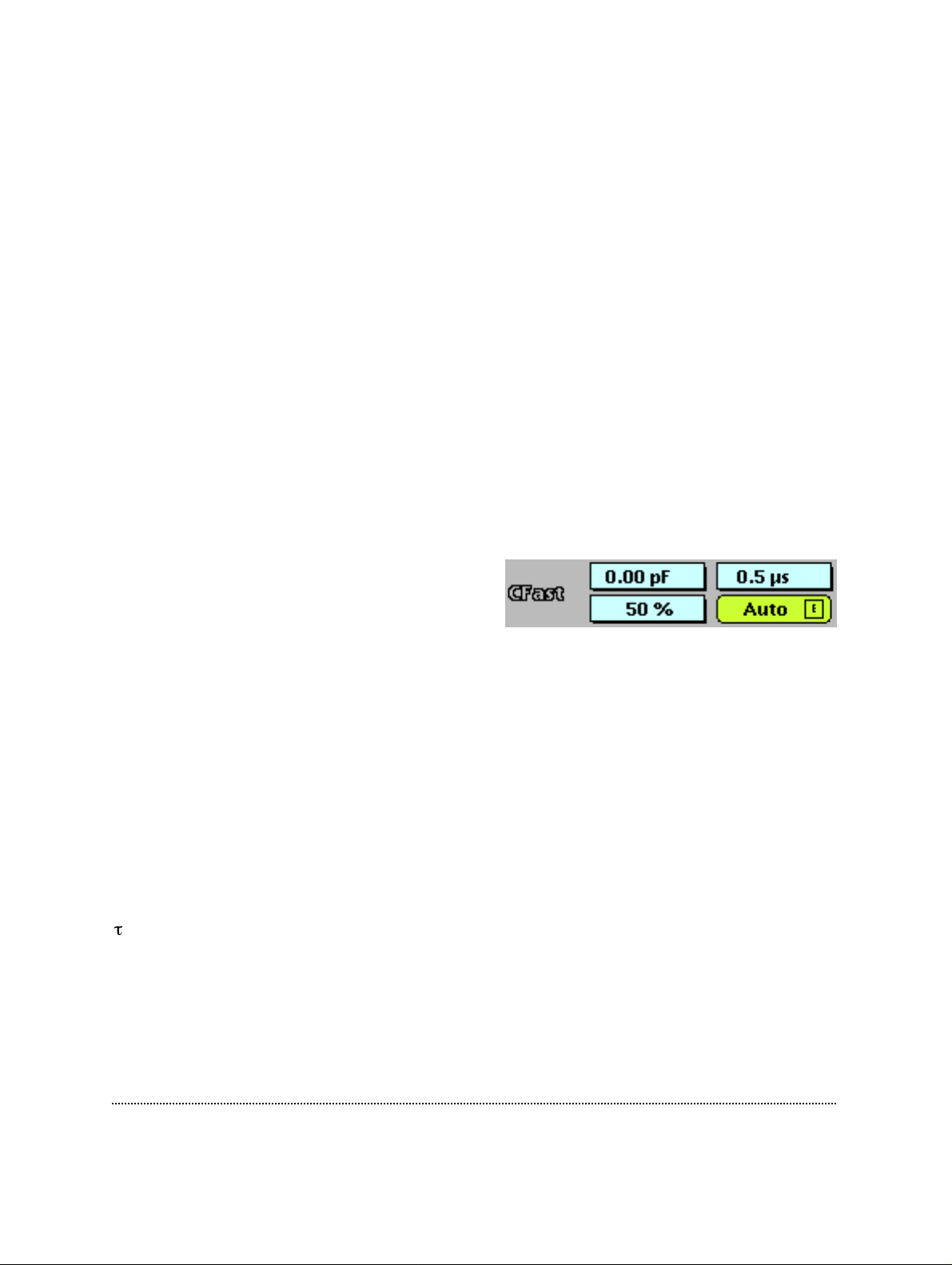
kHz in 0.1 kHz steps (guaranteed accuracy 0.5-15 kHz). Two filter characteristics can
be selected from the pop-up menu:

• Bessel

• Butterworth

The -3 dB point is given in both cases. Bessel is the best characteristic for general use;
the Butterworth response rolls off more rapidly with frequency and is mainly useful
for power spectral analysis. The setting of the Filter 2 control is the actual effective
bandwidth of the series combination of Filter 1 and Filter 2, i.e., the bandwidth of the
signal actually recorded at I-mon 2.

If you want to use an external filter rather than Filter 2, you can proceed as follows:
Connect current monitor 1 (I-mon 1) to the external filter input, feed the filter output
back into one of the AD channels (AD 0...AD 5), and select this channel as input
channel.

Note: Filter 2 is disabled when I-mon 1 is selected. This is to prevent the user to mistake the
Filter 2 bandwidth with the active filter bandwidth used for the sampled data, i.e., Filter 1
bandwidth. To change Filter 2 in this case, select I-mon 2 first.

C-fast: This is used to cancel fast capacitive
currents that charge the pipette and other
stray capacitances (range: 0-15 pF). With
nothing connected to the probe input, cancellation is typically obtained at a setting of
1-1.5 pF due to the residual input capacitance of the current-measuring amplifier.
The compensation can be performed manually by dragging the mouse or typing.
Actually, the setting consists of two components, a completely unfiltered one and a
second one filtered by τ-fast. The program allows you to set the amplitude of the sum
of the two components and the relative contribution of the filtered component (in %).
The %-setting acts like a vernier to τ-fast. A useful way of adjusting the values
manually would be to roughly adjust the value of C-fast at a setting of 50%
contribution and then adjust τ-fast. Thereafter, one can fine-tune the %-setting to
fully compensate capacitive transients. A much easier way of adjusting C-fast and τ-
fast is provided by the automatic compensation feature (simply select the Auto
button; see below).

-fast: This determines the time constant of C-fast (range: 0.5-8 µs in steps of 0.5 µs).

The degree to which the filtered component contributes to the compensation is
specified by the %-setting in C-fast. The value of τ-fast may be adjusted by dragging
the mouse, or typing, or automatically by selecting the Auto function.

E9Screen Software EPC9 Manual 42

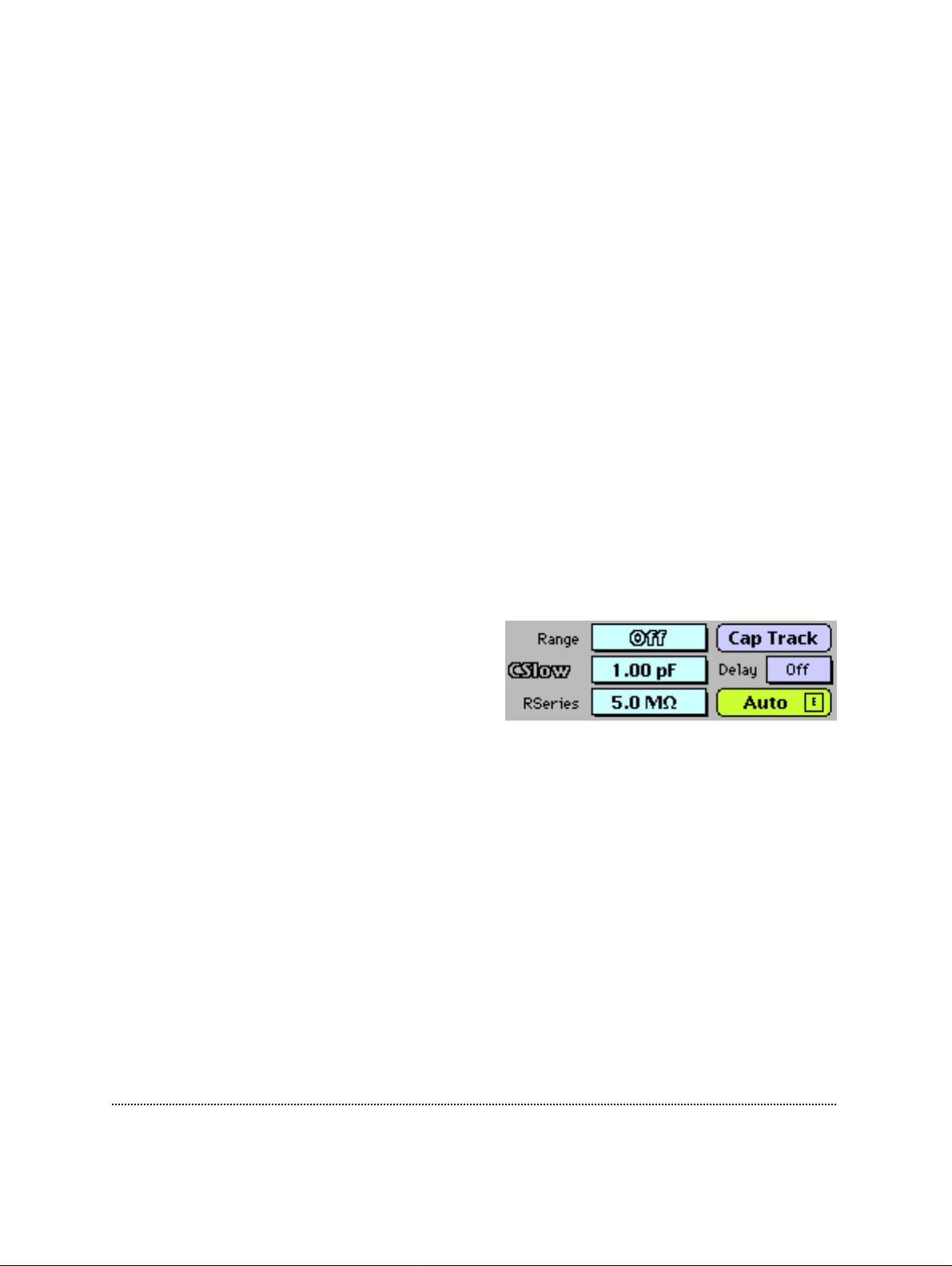
<>: This will select both amplitude and time constant of C-fast. Values for each may
be changed manually depending on whether the mouse is moved horizontally or
vertically.

Auto C-fast: Selection of this button performs an automatic compensation of C-fast
and τ-fast. The procedure uses a routine that applies a number of small pulses (5
mV), averages the resulting currents and fits an exponential to deduce the
capacitance compensation values required to cancel the current. During this
procedure some parameters are changed temporarily: Rs-comp is turned off, the
stimulation is interrupted and the Gain is internally set to an appropriate value (0.2, 2
or 50 mV/pA, depending on the effective gain range). The values are updated in the
respective displays. If the automatic compensation routine fails to converge to ideal
adjustment, the small box in the Auto button (E) will be darkened to indicate the
error. Auto compensation works best with Sylgard-coated pipettes in the cell­attached configuration with C-slow turned off.

The software allows for two ways of making the compensation. The fastest is to use a
look-up table for setting C-fast. In order to do this you have select the option Make C-
fast. If the file created by this procedure (“CFast.epc”) is found in the default
directory (“E9Screen”), the table will be used. Otherwise, when starting E9Screen, a
message will appear that the file could not be found and that the (slower) default
method will be used (iterative compensation).

C-slow Range: Selects the range for slow
capacitance compensation:

• Off - Turns cancellation off.

• 30 pF - Small cells.

• 100 pF - Small and medium-sized cells.

• 1000 pF- Large cells (low and intermediate Gain Range only).

The program will prevent oscillations by limiting compensation according to the
selected range and the effective capacitance values (R-series * C-slow > 5 µs). Selecting
the 1000 pF range will limit the Gain adjustment to a maximum of 20 mV/pA.

Note: If you are using the “Cap. Track” feature to measure small capacitance changes, it is

advantageous to use a higher C-slow range when possible. Counter-intuitive as it
may seem, the digital control of the C-slow circuitry is more precise in higher
ranges, resulting in higher resolution, consistent with the gain range and capacitance.

C-slow: This is used to cancel slow capacitive currents that charge the cell membrane
in the whole-cell configuration. The 30, 100 and 1000 pF ranges actually allow
capacitance values to be compensated in the ranges of 0.12-30 pF, 0.4-100 pF and 4­1000 pF, respectively. The adjustment range is also limited by the program in order

E9Screen Software EPC9 Manual 43

to make the time constant R-series * C-slow greater than 5 µs to prevent oscillations.
The C-slow value may be adjusted manually by dragging the mouse, or typing, or
automatically by selecting the Auto function. Auto-compensation will adjust C-slow
as well as R-series.

R-series: Adjusts the resistance in series with the slow capacitance (range: 0.1 MΩ ­10 GΩ) to determine the time constant of the C-slow transient and also for Rs-

compensation. Adjustment is limited by the capacitance values and the range as
described above. The value can be changed manually by dragging the mouse, or
typing, or automatically by clicking on Auto.

<>: This will select both C-slow and R-series. Values for each are changed depending
on whether the mouse is moved horizontally or vertically.

Auto C-slow: Selecting this function performs an automatic compensation of C-slow
and R-series. These settings are used by the Rs-compensation circuitry as the measure
of series resistance. The procedure uses a routine that applies short trains of square­wave pulses (number and amplitude of these pulses are specified by C-slow Num.
Cycles and C-slow Peak Amplitude), averages the resulting currents and fits an
exponential to deduce the compensation values required to cancel the current (see
Chapter 7. Compensation Procedures on page 59). During this procedure some
parameters are changed temporarily: Rs-comp is turned off, the stimulation is
interrupted and the gain is internally set to an appropriate value (0.2, 2 or 50
mV/pA, depending on the effective gain range). If the C-slow Range is set to Off, it
will automatically be set to the highest possible range, i.e., the 1000 pF range in the
low and medium gain ranges, and the 100 pF range in the high gain range.

Auto-compensation works best when C-fast is canceled beforehand in the cell­attached configuration. The compensation may be improved by alternating cycles of
Auto C-fast and Auto C-slow. If the compensation fails, the small box in the Auto button
(E) will be darkened to indicate the error. Continuous Auto-compensation can be
performed by selecting Cap. Track option, see below.

Note: It is necessary that reasonable estimates for C-slow and R-series are supplied before

the Auto C-slow is started, otherwise the auto-compensation may fail.

Cap. Track: Selecting this button will perform repetitive Auto C-slow compensation.
Clicking on Cap. Track again will turn it off.

Note: The “Output Cap. Track” option in the EPC9 menu determines whether the

capacitance and G-series values are output as voltages on the DA channels 0 and 1.
If selected, the C-slow value is available at DAC 0, and the G-series value (1/R­series) is available at DAC 1. The scaling for G-series is 100 nS/V; scalings for C­slow are 0.5, 5 or 50 pF/V for 30, 100 and 1000 pF ranges, respectively. The DAC
values will be reset to zero when activating “Reset”. Make sure that the trigger DAC
is neither DAC 0 nor DAC 1 when you want to activate "Output Cap. Track".

E9Screen Software EPC9 Manual 44

Delay: This determines how many seconds to wait before the next auto­compensation is started. With short delays (e.g., 1 ms), membrane capacitance will be
tracked at rates of >10 Hz (depending on the Macintosh model).

Note: You can increase the rate of Cap. Track (about two-fold) when closing the

Oscilloscope.

Rs-comp: The series resistance compensa­tion corrects for membrane voltage errors
under conditions of high access resistance between pipette and cell interior (see see
Chapter 7. Compensation Procedures on page 59). The amount of compensation can
be changed by dragging the mouse or typing (range 0-95%). The compensation is
based on the value of R-series and will be effective only when Rs-comp is not Off, i.e.,
set to a speed value. The following settings determine the speed of feedback
compensation:

• Off - Turns compensation off.

• 100 µs - Slow compensation.

• 10 µs- Fast compensation.

• 2 µs - Very fast compensation.

The choice of speed depends on the recording time constant and the degree of
compensation desired, as described in Chapter 7. Compensation Procedures on page

59. Fast Rs-compensation requires more critical adjustment of the controls but
provides the maximum voltage-clamp speed. In fast modes, Filter 1 will be

automatically switched to its HQ-30 kHz setting. In Current Clamp mode, Rs-comp
will act as a bridge compensation.

Test Pulses: Test pulses are added to the holding
potential and applied to the pipette; the current
responses are sampled and displayed. Test pulses are
applied at maximal rates depending on the durations
specified.

Amplitude / Duration: Duration and amplitude of built-in test pulses can be
specified in the dialog. The minimum pulse duration is 1 ms with 100 points
sampled per pulse, i.e., the sampling interval is 1/100 times the pulse duration.

Stimulus: The stimulus can be filtered (2-pole Bessel)
to reduce the amplitude of fast capacitance transients
when the speed of potential changes is not critical.
Two settings are available:

• 2 µs • 20 µs

E9Screen Software EPC9 Manual 45

Usually a setting of 20 µs is sufficient, unless very fast currents such as Na+ currents
are studied.

External: The external Stim. Input is scaled by an editable factor (range: ±0-10x), to
allow for different external stimulators. It is strongly recommended to set External to
Off (i.e., equal to zero), if no external stimulator is connected to the Stim. Input. This
will prevent pick-up of external noise. Please note that the internal V-membrane is not
affected by changing the external scale factor. If the user sets the holding potential
externally (e.g., with a stimulator or another computer), then the scaling will affect
the holding potential.

Gain: Sets the gain of the oscilloscope display.
Clicking on the arrow icon will cause the
sweeps to be centered in the oscilloscope.

Close: Closes the oscilloscope display. With the oscilloscope closed the controls for
sound encoding of R-membrane and Current-Clamp Speed (EPC9 version “C” and later)
become accessible. There will be no test pulse while the oscilloscope remains closed.

Overlay: Acquired sweeps will be overlayed if this switch is selected.
Clear: Wipes the oscilloscope display.
Leak Sub.: This controls a hardware leak

compensation which uses the inverted and
scaled stimulus signal and adds it to the
current monitor outputs. Leak can be adjusted manually by dragging the mouse, or
typing, or automatically by clicking on Auto. The maximal values attainable depend
on the Gain Range. They are 2 nS, 200 nS and 20 µS for high, medium, and low
ranges, respectively.

Auto: Determines and corrects for the leak conductance automatically.
Track: Continuously updates the leak compensation, thus tracking changes in

membrane conductance.

Hidden Controls

Some rarely used controls are hidden behind the oscilloscope display. They can be
accessed by closing the oscilloscope display:

E9Screen Software EPC9 Manual 46

Sound Settings: Sensitivity (Hz/MΩ) and volume
(in %) of the sound encoding of R-membrane can be

Hz/MΩ Rmem

Sound

specified here. To enable the sound option press the
Sound button.

CC Fast Speed: Clicking on this button enables the fast current­clamp mode (only version “C” and later versions of the EPC9).
For details see Chapter 6. Operating Modes on page 54).

Volume

100

100 %

Gentle CC-Switch: This control selects between the

Gentle CC-Switch: ON

two alternate modes of switching between voltage
and current clamp and back.
When selecting Gentle CC-Switch: On, I-hold will be set to inject the holding current
required to keep the membrane voltage constant while switching to current clamp
mode. Thus, V-mon will be identical to the original V-membrane commanded under
voltage clamp. In analogy, upon returning to voltage clamp, V-membrane will be set
according to the membrane potential under current clamp and rounded to the next 2
mV.
When selecting Gentle CC-Switch: Off, I-hold will be set to 0 pA when switching to
current clamp mode.

Last V-membrane: Quite often, the membrane potential under
current clamp will have changed, and when returning to voltage
clamp, V-membrane will possibly differ from that set before switching to current­clamp mode. Last V-membrane can then be used to conveniently restore the original
V-membrane value.

CC-range: Two current clamp scaling ranges can be

CC-range: 1pA/mV

selected: 1 and 10 pA/mV (with the exception of the
EPC9 version “A” and “C”, which have a fixed CC-scaling of 1 pA/mV). When the
CC-scaling is set to 1 pA/mV, a command pulse of 1 mV gives rise to 1 pA inCurrent
Clamp mode. This relationship of 1 and 10 pA/mV holds regardless of the Gain
setting. The maximal output current inCurrent Clamp mode is 1 and 10 nA,
respectively.

Relative Value: This button is useful when recording

Relative Value

macros. A change of any value will be recorded as a
relative change, e.g. if you hyperpolarize the holding potential from -60 to -70 mV
while recording a macro, a step of -10 mV will be recorded (see description of Macros
at the beginning of the subchapter Main Controls).

E9Screen Software EPC9 Manual 47

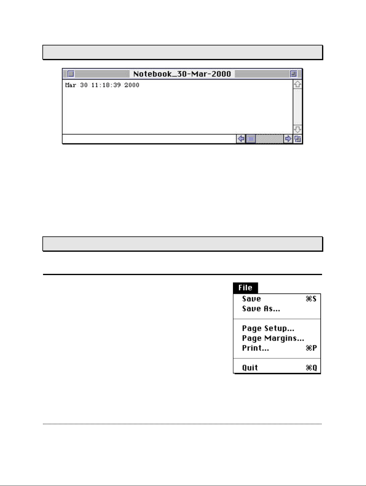
Notebook Window

The Notebook window is used to display printed output of the program, such as error
messages or information about calibration and diagnostic data, for example. The
content of the Notebook can be stored in a memory file; its maximal size can be to be
specified in the drop-down menu Notebook. One can modify text in the Notebook just
as in any other text file. One can add further information to the text file or delete
messages that should not be stored. While in the Notebook window you can copy to
and paste from the clipboard. Thus, you can exchange text with other applications,
such as spreadsheets.

Drop-Down Menus

File Menu

Save: Saves the Notebook content to disk.
Save As…: Asks for a filename before saving.
Page Setup…: Prompts for printer page format.
Page Margins…: Sets the page margins for printing.
Print…: Prints the Notebook content. If some text is se-

lected (i.e., highlighted), only that text selection is
printed.

Quit: Exits E9Screen.

E9Screen Software EPC9 Manual 48

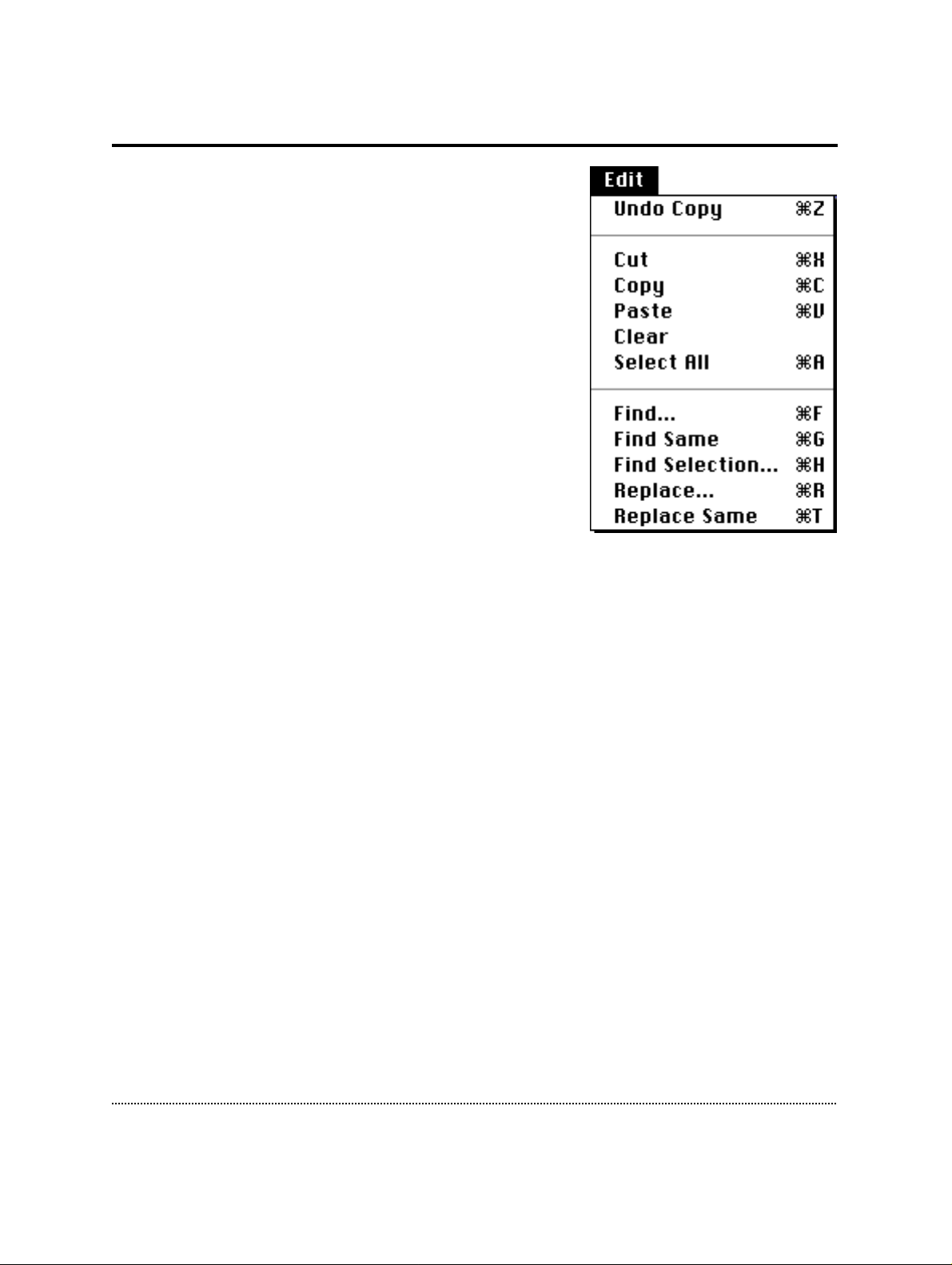
Edit Menu

The Edit menu is not used by E9Screen except for text
manipulation of the Notebook content. All entries are
normally disabled unless the Notebook is selected. The
menu entries conform to the standard Macintosh
functions.

The Cut, Copy, and Paste commands copy the text
selection to and from the clipboard. Clear removes the
text.

Find…, Find Same, Find selection…, Replace…, and
Replace same perform the obvious functions.

E9Screen Software EPC9 Manual 49

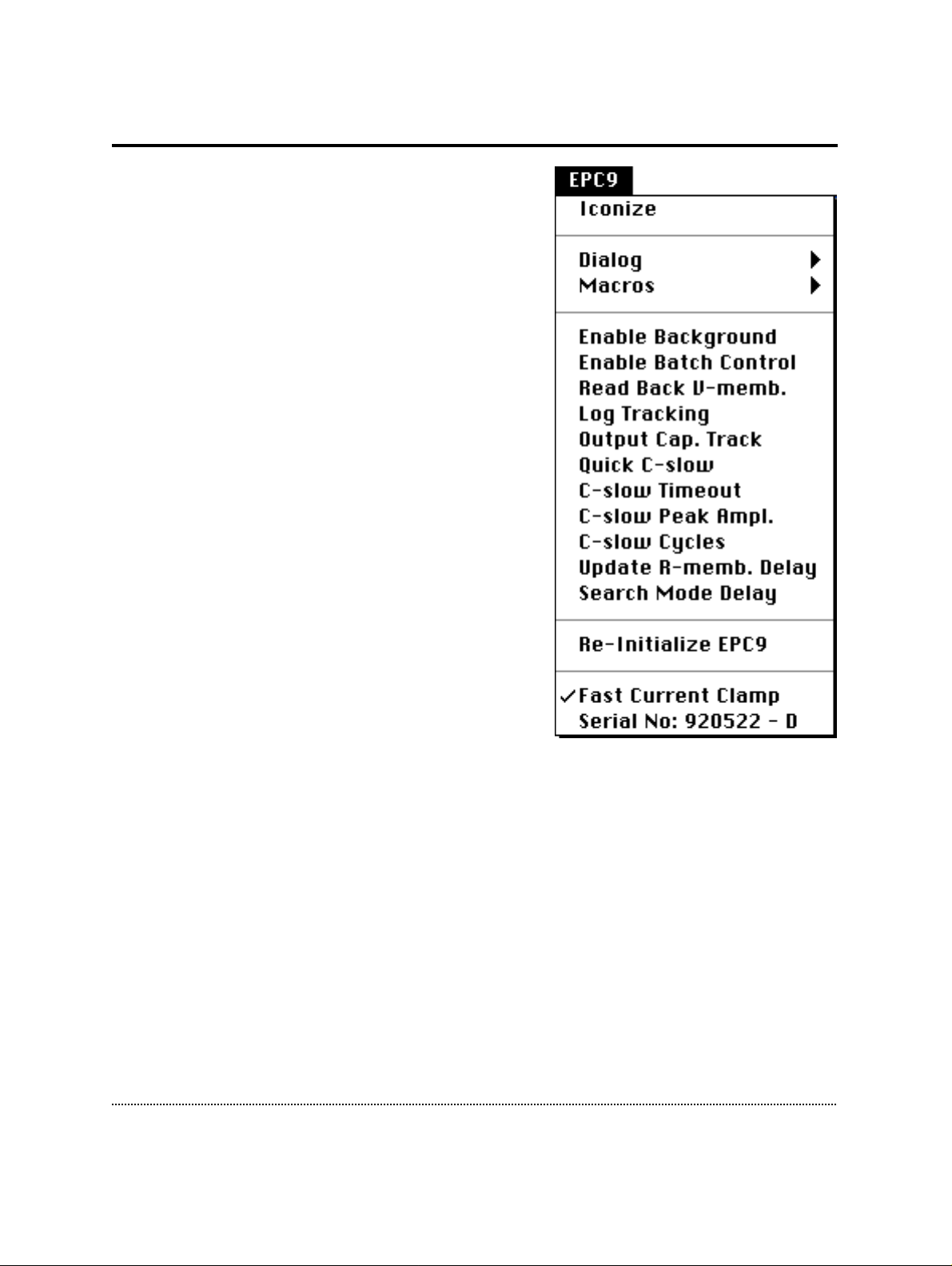
EPC9 Menu

Iconize: Collapses the window and leaves the
title bar of the window on the desktop.

Dialog: Selects a submenu for the Amplifier dialog
window. The following functions are available:

• Load…: Loads a saved dialog window.

• Save…: Saves a modified dialog window.

• Save as PICT…: Saves window as Pict file.

• Reset: Resets the dialog window to default.

• Enable Dragging: Enables the dragging fea-

ture for most amplifier controls.

Macros: Selects a submenu for macro functions.

• Load…: Loads a saved macro file.

• Save…: Saves a macro file.

• List: Prints the current macros in the Note-

book.

• Start Recording: Starts macro recording.

• Execute while recording: If checked, the

actions will be executed. Otherwise, the
actions will be logged to the macro but not
change any settings.

EPC9 Help: Enters the online Help mode for EPC9 functions.
Enable Background: Enable E9Screen to run in the background, i.e., when it is not

the front application. Thus, E9Screen will continue to perform Cap. Track and to scan
the clipboard for batch file instructions (see Appendix I).

Enable Batch Control: Enables E9Screen to communicate with other applications via
batch files (see Appendix I).

Read Back V-memb.: Required when using E9Screen in combination with another
acquisition program. When active, E9Screen will read the momentary V-membrane
when the user switches from another application to E9Screen. This allows E9Screen to
know the V-membrane this other application has set.

E9Screen Software EPC9 Manual 50

Log Tracking: Writes the updated values of C-slow, G-series, and G-leak to the
Notebook when capacitance tracking is on.

Output Cap. Track: Outputs the values of C-slow and G-series as analog voltages to
DA 0 and DA 1, respectively.

Quick C-slow: Selects an alternate procedure for Auto C-slow compensation. It
speeds up repetitive compensations, as it does not switch the gain, filter settings, etc.
This option does not check as thoroughly for proper convergence and will
sometimes adjust C-slow and R-series when the normal C-slow compensation would
have returned an error. Use this option with caution.

C-slow Timeout: The time after which E9Screen will terminate an Auto C-slow.
C-slow Peak Amplitude: The amplitude of the voltage pulses used to compute C-

slow and G-series.

C-slow Cycles: The number of voltage pulses used to compute C-slow and G-series.
Update R-membrane Delay: This option sets the refresh rate of R-membrane in the

EPC9 window. To suppress R-membrane calculation and update, enter a large value.
Search Mode Delay: The Search Mode (see Chapter 6. Operating Modes on page 58 )

is essentially a repetitive Auto-V0 procedure at a holding potential of 0 mV. The delay
specifies at what rate Auto-V0 is performed.

Re-Initialize EPC9: This is used to restart the AD/DA interface; e.g., when E9Screen
was started with the interface being turned off.

Fast Current Clamp: Selects the fast current-clamp mode (only version “C” and
later versions of the EPC9). For details see Chapter 6. Operating Modes on page 54).

Serial No: [Serial #] - [EPC9 version]: Displays the serial number and version of the
connected (and initialized) EPC9 amplifier.

E9Screen Software EPC9 Manual 51

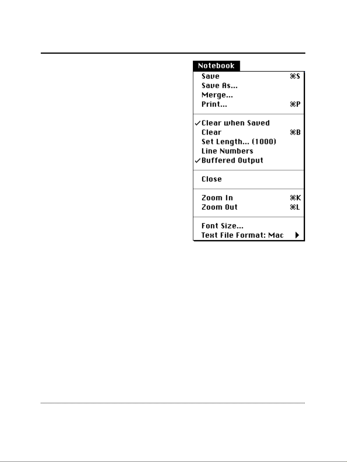
Notebook Menu

Save: Saves the Notebook under its default
name: “Notebook_Date”.

Save as…: Asks for a filename before saving.
Merge...: Appends the present Notebook to an

existing one.
Print…: Output content of Notebook to a

printer. If some text is selected (i.e.
highlighted), only that text selection is printed.

Clear when Saved: Automatically clears the
Notebook after the present content is saved to
disk.

Clear: Clears Notebook.
Set Length…: Specifies maximal number of

text lines in the Notebook. The maximal number
of lines is given in parentheses.

Note: Large notebook buffers require a lot of

CPU time and RAM. If execution time
during acquisition is an issue, the buffer size should be kept small or the “Buffered
Output” should be turned off. The RAM requirement is 260 bytes per line. Thus,
1000 lines consume 260 kbytes.

Line Numbers: Shows line and column numbers in the Notebook.
Buffered Output: Keeps all text written to the Notebook in the buffer. If deselected,

information printed to the Notebook window will not be saved.

Open/Close: Opens or closes a Notebook window.
Zoom In/Out: Expands and shrinks the Notebook window.
Font Size…: Specifies the font size of the Notebook text.
Text File Format: Specifies in which format the Notebook text is saved:

• Mac - Line Feed

• DOS- Line Feed + Carriage Return

E9Screen Software EPC9 Manual 52

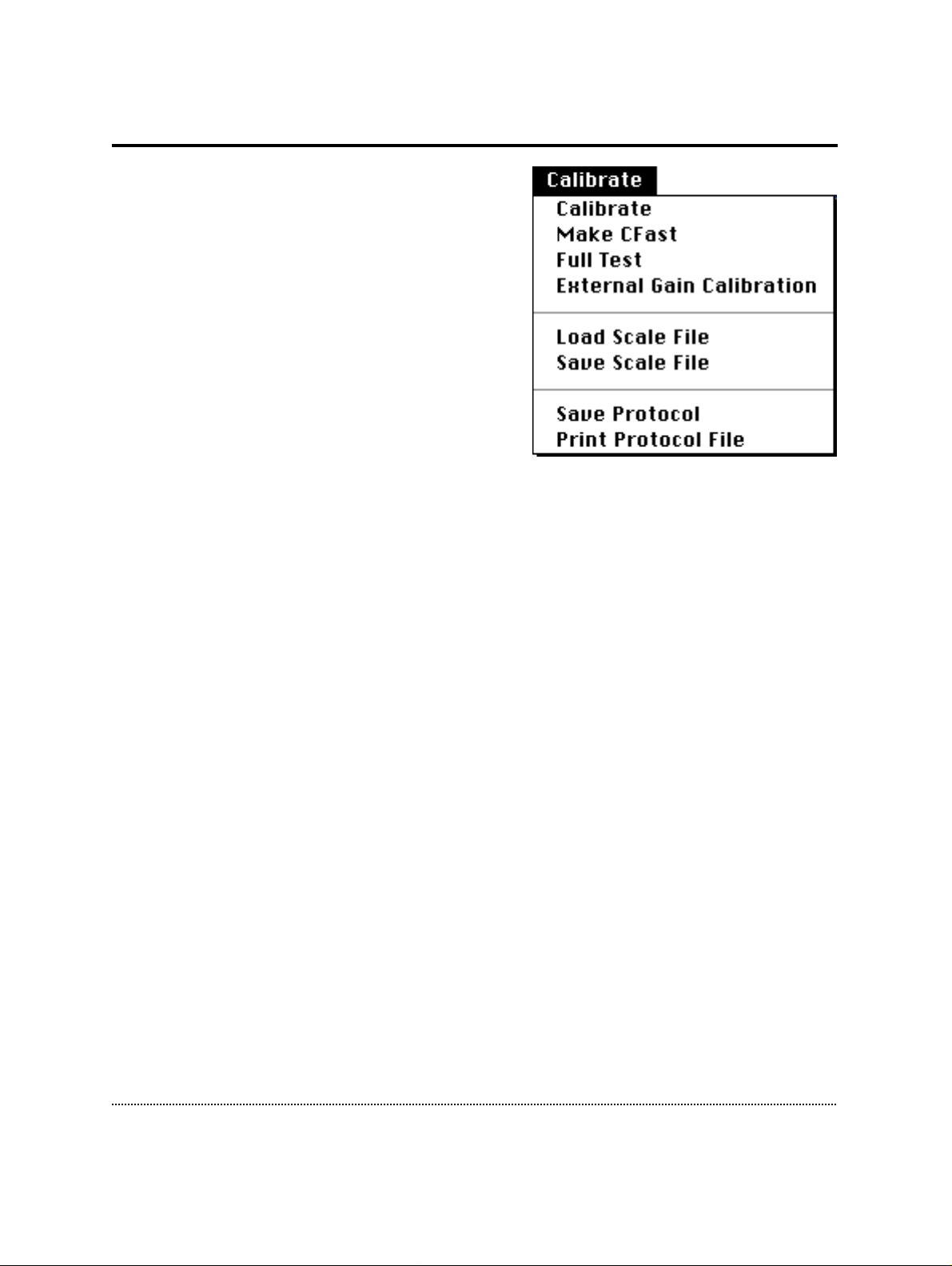
Calibrate Menu

Calibrate: Performs a full calibration of the
EPC9. The result of this calibration may be
stored as a “SCALE.EPC” file. This file contains
the settings of the digital switches and controls
of the amplifier. These are unique to the
amplifier and cannot be used for another EPC9.
A calibration should be performed in intervals
of about 6 months or whenever the frequency
response of the amplifier is not accurate or
offset currents become noticeable. Depending
on the speed of the computer, the calibration
process takes 5-10 minutes.

Note: Calibrations should be performed after

amplifier and probe have reached normal operation temperature (i.e., powered up for
about 15 min.utes)

Make C-fast: Generates a look-up table for Auto C-fast compensation. The file is
loaded automatically if it has the name “CFAST.EPC” and is found in the E9Screen
folder.

Full Test: Performs a hardware test. This generates a list of diagnostic values. This
may be used to inform the manufacturer (HEKA) about the condition of the EPC9. If
you have any doubts about your EPC9 test, please contact HEKA to find out whether
or not it needs to be serviced.

External Gain Calibration: This option allows to use an external precision resistor to
improve the internal, automatic gain calibration. Usually there is no need to perform
an external gain correction, but some users may chose to do so. A gain correction
factor can be given for each gain range, i.e., low, medium, and high gain. Thus, this
enables a “user specified” gain correction factor for matching the computed the R­membrane value with a calibration resistor.

Load / Save Scale File: Loads or saves calibration files.
Save Protocol: Saves the protocol file of a Full Test.
Print Protocol File: Prints the protocol file of a previously saved Full Test.

E9Screen Software EPC9 Manual 53

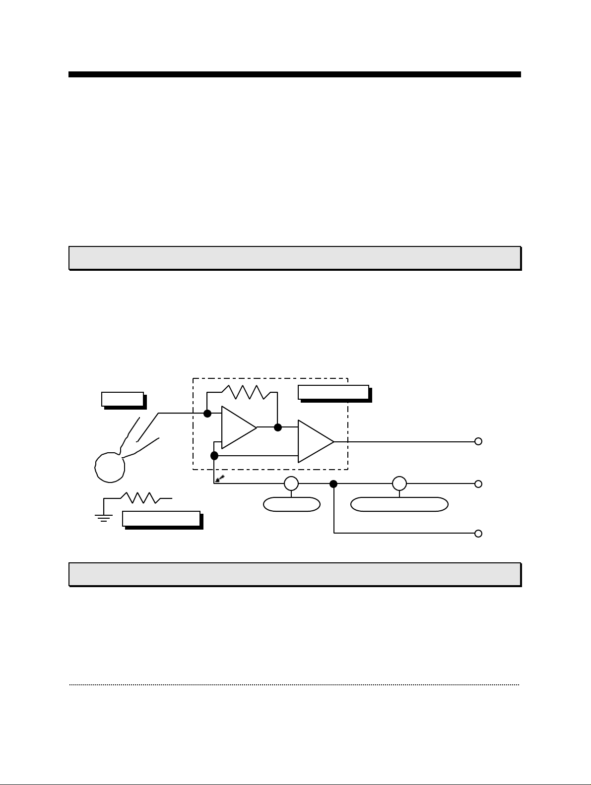
6. Operating Modes

The EPC9 is fundamentally an instrument for measuring small electrical currents. It
uses a current-to-voltage (I-V) converter circuit to convert the currents to an analog
voltage, which is then made available at the current monitor outputs for display or
recording. At the same time that pipette currents are being recorded, the potential
must be specified, and the various operating modes of the EPC9 correspond mainly
to different ways of controlling that potential.

Voltage-Clamp Mode

This is the basic patch-clamp mode, and is implemented by the circuitry shown in
the figure below. The pipette potential is derived from the signal applied to Stim. In,
with a variable offset added from the V-membrane control. The sum of these two
sources is displayed and monitored as the V-mon signal. Before being applied to the
pipette a further variable offset is added from V0 (which includes the value of LJ, see
Chapter 7. Compensation Procedures on page 59).

Pipette

Ref. Pot.

V0-Offset V-memb. + Stim. In

Bath Electrode

IV Converter

Current
Monitor

Stim. In

Σ Σ

Voltage
Monitor

Current-Clamp Mode

In the Current Clamp mode, the feedback is employed between the current monitor
signal and the pipette potential (see figure below). The feedback acts rapidly (with a
time constant of about 30 µs) to keep the current at zero by varying the pipette
potential appropriately; in this way, a high-impedance voltage follower is created,
with the output voltage available at the V-mon output. The original V-membrane

Operating Modes EPC9 Manual 54

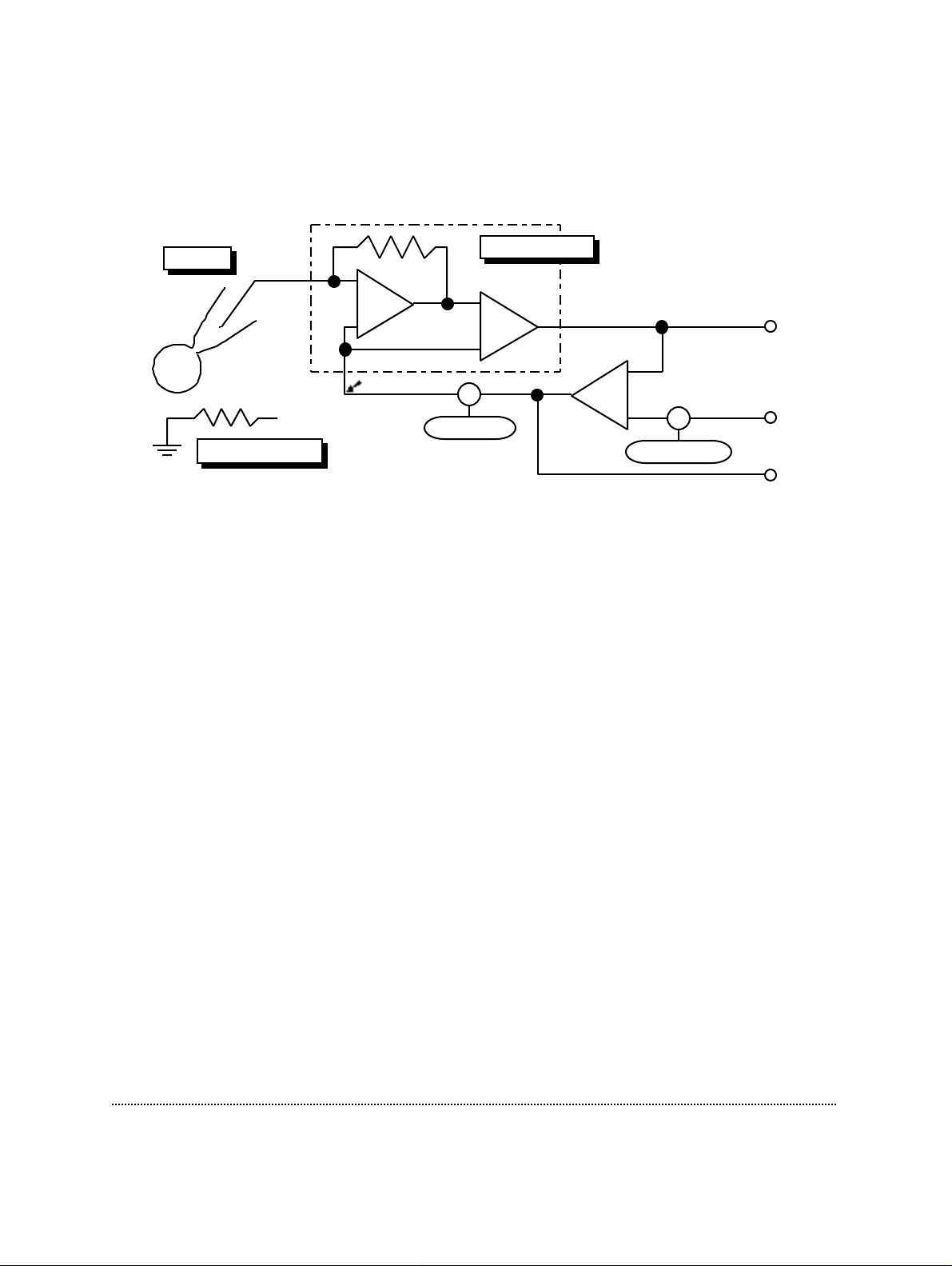
viewport now becomes an I-membrane display and may be used to inject a steady
command current through the action of the feedback amplifier. In E9Screen, the
membrane potential is shown in the I-mon display; in Pulse, the I-mon display is
converted to V-mon).

Pipette

Ref. Pot.

V0-Offset

Bath Electrode

IV Converter

Σ

Σ

I-membrane

Current
Monitor

Stim. In
Voltage

Monitor

You can use the Current Clamp mode to measure the resting potential or spontaneous
action potentials in a whole-cell recording, and the membrane potential will be
shown on the V-mon display. A commanded current can be injected while the pipette
potential is measured. The commanded current is determined by the sum of voltages
from the Stim. In signal and the I-membrane control.

Two current clamp scaling ranges can be selected: 1 and 10 pA/mV (with the
exception of the EPC9 versions “A” and “C” which have a fixed CC-scaling of 1
pA/mV). When the CC-scaling is set to 1 pA/mV, a command from the Pulse

Generator or from the I-membrane control that would give rise to 1 mV in the Voltage
Clamp mode instead gives rise to 1 pA in the Current Clamp mode. This relationship

of 1 and 10 pA/mV holds regardless of the Gain setting. The polarity is the usual
one, in which positive stimuli result in currents flowing out of the pipette.

Note: The “Gain” settings are restricted to the intermediate range, i.e. 0.5-20 mV/pA, in

current-clamp mode.

When switching from voltage-clamp to current-clamp mode, I-membrane will be set
to whatever is needed in order to keep the membrane voltage at the value that was
commanded in voltage clamp. Likewise, upon returning to voltage clamp, V-
membrane will be maintained. Thus, switching modes will be as gentle as possible,
since the membrane potential will always remain constant. If you wish to switch
modes under different conditions, it is convenient to program a macro to, for
example, set a holding current value immediately after switching to current clamp.
The EPC9 allows the functions of C-fast and Rs-comp to be on when entering current­clamp mode. C-fast then becomes a “negative capacitance” adjustment and Rs-comp
becomes a “bridge” adjustment.

Operating Modes EPC9 Manual 55

The main problem with current-clamp settings is stability, as the feedback loop will
oscillate when C-fast is set to its true value; the loop expects at least a small amount
of uncompensated C-fast for a phase lead at high frequencies. The EPC9 software will
assume that the user has compensated C-fast correctly, and in the process of
switching to current-clamp mode, it will set its value slightly lower (0.5 pF) to
optimize the speed of recording. The Current Monitor output can be used to monitor
the currents being passed, with the Gain control determining the sensitivity.

The new version “C” of the EPC9 hardware (and later verisons):

In the new EPC9 versions the current-clamp circuitry has been improved to better
follow rapid changes in membrane potential, such as in neuronal action potentials. In
the current-clamp mode a feedback circuit causes the effective input resistance of the
EPC9 headstage to be greater than 10e11 Ω. The speed of the feedback loop
determines the effective input capacitance of the amplifier; a high capacitance can
cause the time course of the action potential to be slowed. The capacitance of the
electrode, and to some extent the amplifier, can be neutralized by the C-fast setting,
which acts as a capacitance neutralization adjustment in the current-clamp mode.
However, like capacitance neutralization settings on conventional microelectrode
amplifiers, excessive capacitance neutralization can result in oscillation and
potentially the destruction of the cell membrane. The best way to use the C-fast
control is to first adjust it in the voltage-clamp mode, e.g., by using the Auto button; it
is then automatically adjusted to neutralize all but the amplifier input capacitance
when you switch to current-clamp mode.

The current-clamp circuitry now has two speed settings (which can be toggled by a
button that is normally hidden behind the oscilloscope window; it can be seen when
closing the oscilloscope). At the fast setting, the effective input capacitance of the
headstage is 2 pF. This amount of capacitance will cause little loading of most cells. If
desired you can neutralize a fraction of this capacitance as well by increasing the C-
fast setting by up to 2 pF from its initial value. Overshoot or ringing of the response
will occur as you approach complete compensation.

The fast current-clamp setting must be used with some caution because if C-fast is
grossly misadjusted, either by being too high (i.e., overcompensation) or too low,
oscillation may occur. The fast current-clamp mode may also oscillate in situations
where the impedance of the electrode and the cell are low, below about 5 MΩ at a
frequency of 10 kHz. Thus oscillation may occur when the pipette has a resistance
below 5 MΩ and is open to the bath solution, or in recording from a cell with
substantial membrane capacitance when the series resistance is less than 5 MΩ.

In the slow setting, the current-clamp system is more stable, but an effective input
capacitance of 24 pF is produced. Because this value is larger than the range of the C-
fast controls, misadjustment of C-fast will not cause oscillation; the amplifier is also

Operating Modes EPC9 Manual 56

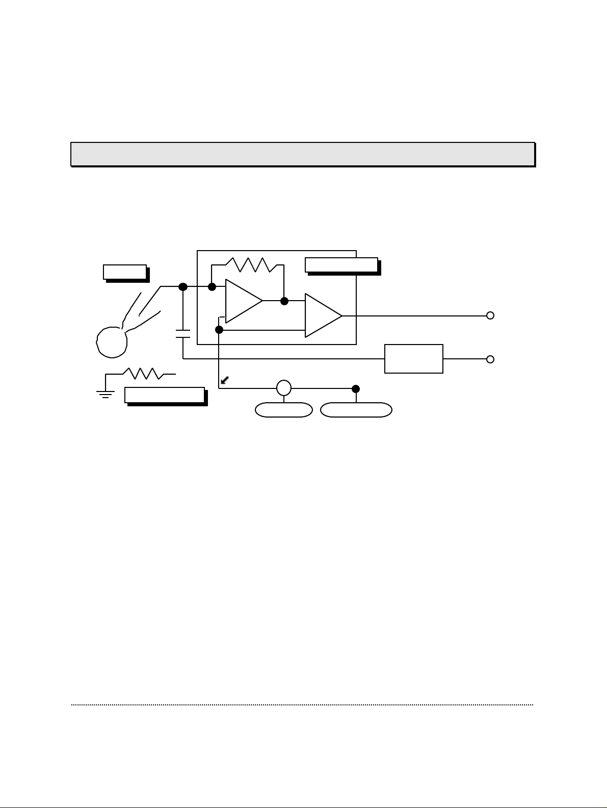
stable with pipette and series resistance down to 1 MΩ. The large capacitance will
however produce an extra load on small cells, slowing the time course of membrane
potential changes.

Test Mode

This mode is only available in E9Sreen. It is very much like the voltage-clamp mode
(see figure below) except that the Test Integrator signal is used to inject small test
currents into the I-V converter input. Internal stimulation can be used for this
purpose by connecting DA 2 (Test Output) to the Test Input.

Pipette

Bath Electrode

Ref. Pot.

V0-Offset

Σ

IV Converter

V-membrane

Test

Integrator

Current
Monitor

Test. In

The scaling of the current that is injected is fixed at approximately -100 pA per volt
applied at the Test Input. This scaling is independent of the Stim. scaling setting. The
exact scaling is measured in the calibration program and is stored in the “Scale.epc”
file. The signal is not DC-coupled, but square waves of >20 Hz, pulses >30 ms in
duration, and sine waves at >1 Hz are reproduced faithfully.

Note: The test integrator inverts the externally-supplied signal. For accurate frequency

response and to avoid degrading the sensitivity of the I-V converter, the test currents
are injected through a capacitor (rather than a resistor) into the probe's input
terminal. The applied signal is integrated by an auto-zeroing integrator before being
applied to the capacitor. The integrator may require several seconds of recovery time
when a signal with a substantial DC component is applied to the input.

The Test mode is particularly useful for measuring the step response of the entire
recording system, which is a necessary step in high-resolution channel analysis, as
described by Colquhoun and Sigworth (1995). The current-injection circuitry has a
useful bandwidth greater than 100 kHz in the high range of gain settings and can be
used for quantitative measurement of the step response.

Operating Modes EPC9 Manual 57

Search Mode

In the EPC9, this mode has no special analog circuitry. Rather, it is a software
emulation of the traditional search mode found in the EPC7 amplifier. The EPC7
accomplished the search mode by analog circuitry in order to ease the adjustment of
the zero-current potential V0. The EPC9 does not require special analog circuitry, as
the software provides for an easy way of doing this. The Search mode of the EPC9
simply forces V-hold to 0 mV and invokes the Auto-V0 procedure (at the rate specified
by Search Mode Delay in the EPC9 menu), which will adjust the offset potential
automatically in order to zero the current. Thus, the search mode is simply a
repetitive update of V0.

Operating Modes EPC9 Manual 58

7. Compensation Procedures

Series Resistance Compensation

In whole-cell voltage-clamp recording, the membrane potential of the cell is
controlled by the potential applied to the pipette electrode. This control of potential
is not complete, but depends on the size of the access resistance between the pipette
and the cell interior, and on the size of the currents that must flow through this
resistance. This access resistance is called the series resistance (Rs) because it

constitutes a resistance in series with the pipette electrode. Part of the series
resistance arises from the pipette itself, but normally the major part arises from the
residual resistance of the broken patch membrane, which provides the electrical
access to the cell interior. In practice, we find that the series resistance usually cannot
be reduced below a value about two times the resistance of the pipette alone.

Series resistance has two detrimental effects in practical recording situations. First, it
slows the charging of the cell membrane capacitance because it impedes the flow of
the capacitive charging currents when a voltage step is applied to the pipette
electrode. The time constant of charging is given by τu = Rs x Cm, where Cm is the

membrane capacitance. For typical values of Rs = 5 MΩ and Cm = 20 pF, the time
constant is 100 µs. This time constant is excessively long for studying rapid, voltage-

activated currents such as Na+ currents in neurons, especially since several time
constants are required for the membrane potential to settle at its new value after a
step change. The second detrimental effect of series resistance is that it yields errors
in membrane potential when large membrane currents flow. In the case of Rs = 5

MΩ, a current of 2 nA will give rise to a voltage error of 10 mV, which is a fairly
large error; for studying voltage-activated currents, errors need to be kept to ~2 mV
at most.

Electronic compensation for series resistance in voltage-clamp systems has been in
common use since the days of Hodgkin and Huxley. The principle of the
compensation in the case of a patch clamp is that a fraction of the current monitor
signal is scaled and added to the command potential (correction pathway, see figure
below). When a large current flows in the pipette, the pipette potential is altered in a
way that compensates for the potential drop in the series resistance. This
arrangement constitutes positive feedback, and can become unstable when
overcompensation occurs.

Compensation Procedures EPC9 Manual 59

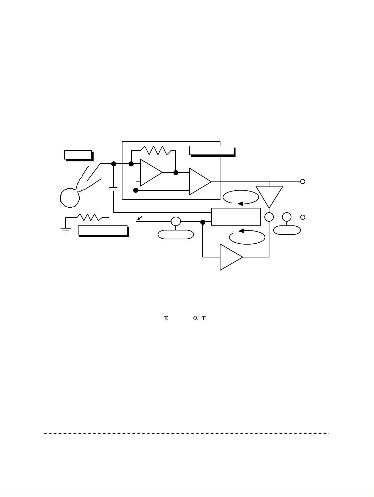
The EPC9 incorporates additional circuitry to allow capacitance transient
cancellation to occur while Rs-compensation is in use (see Sigworth, Chapter 4 in

Single Channel Recording). This is shown as the prediction pathway in the figure
below, and it accelerates the charging of the membrane capacitance by imposing
large, transient voltages on the pipette when step changes are commanded (this is
sometimes called “supercharging”). These voltages would occur due to the action of
the correction pathway alone as the large capacitive charging currents elicit pipette
voltage changes; however, when these currents are cancelled by the transient
cancellation, their effect must be predicted by the cancellation circuitry: hence the
prediction pathway.

Pipette

Bath Electrode

Ref. Pot.

V0-Offset

Σ

IV Converter

Transient Gen.

Corr. Loop

C-slow

Pred. Loop

Current
Monitor

Stim. In

Σ Σ

V-hold

Together, the two parts of the EPC9 Rs-compensation circuitry cancel the effects of a
fraction of the series resistance. This means that the charging of the membrane

capacitance is accelerated, with a time constant under compensation of

= 1 −

( )

c

u

where τu is the uncompensated time constant. Similarly, the voltage errors due to
membrane currents are also reduced by the factor (1-α). The fractional compensation

α is determined by the setting of the %-comp control on the EPC9 software. For

proper compensation, however, the circuitry needs to have an estimate of the total
series resistance (for the correction pathway), and both the series resistance and
membrane capacitance must be known for the capacitance transient cancellation (C-
slow) circuitry. In the EPC9, the estimation of series resistance has been combined
with the transient cancellation, in that the Rs control has a dual effect. Its setting

affects both the kinetics of the transient cancellation and the scaling of the correction
feedback signal. This means that in practice the estimation of the series resistance

Compensation Procedures EPC9 Manual 60

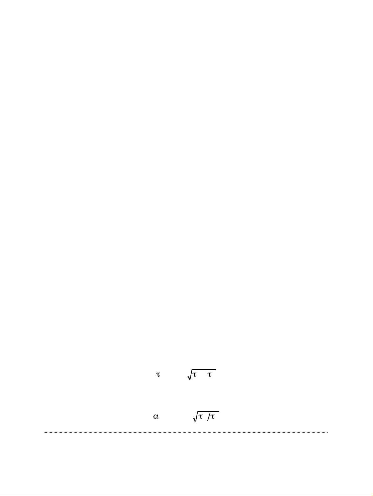
consists of adjusting C-slow and R-series to cancel the transient currents due to the
cell membrane capacitance. Once this has been done, the relative amount of Rs-

compensation can then be selected with the %-comp control.
Theoretically, it is desirable to compensate as much of the series resistance as

possible. In practice, however, a degree of compensation above 90% can involve
considerable technical problems, and in some recording situations a value below
90% is preferable. To illustrate one technical problem, consider the case when a 100
mV potential change is commanded and 90% compensation is in use. This degree of
compensation means that the cell membrane capacitance will be charged 10 times
faster than normally. The rapid charging is accomplished in the compensation
circuitry by forcing the pipette potential to (very transiently) reach a potential of 1V.
The resulting large current causes the membrane capacitance to charge quickly to its
final value of 100 mV. In general, when a voltage step of size ∆V is commanded, the
pipette potential actually receives an initial transient of size ∆V / (1-α) due to the
compensation effect. The technical problem comes from the fact that the maximum
pipette potential excursion in the EPC9 is about ±1.2 V, implying that 90%
compensation can be used for steps only up to about 120 mV in amplitude. Overload
of amplifiers (obvious in practical use due to the loss of proper transient cancel­lation) will occur if larger pulses are applied, unless the %-comp setting is reduced.

The degree of Rs-compensation is also limited by stability considerations. Stable Rs­compensation requires that the C-fast control is properly set to cancel the fast

capacitance transients; when the series resistance is high, say above 10 MΩ,
misadjustment of C-fast can easily cause oscillation. In cases where Rs is this size or

larger, it is often advisable to use the slower settings of the Rs switch which, in
slowing down the speed of the compensation feedback, makes it less susceptible to

high-frequency oscillations. In cases where Rs is relatively small, on the other hand,
it is sometimes not possible to use full 90% compensation because of the limited

speed of the compensation feedback, even in the fastest, 2 µs setting of the switch.
This problem arises when the time constant τu is smaller than about 100 µs, and

comes from the fact that compensated membrane time constant τc cannot be made
smaller than a value that depends on the speed of the Rs-compensation feedback. If
you turn up the %-comp control to try to obtain a smaller τc, you will observe
overshoot or ringing in the current monitor signal, due to an overshoot in the

membrane potential. The minimum value for τc is given approximately by

c(min)

=

−

u

f

where τf is the effective time constant of the feedback loop. The corresponding
maximum α values are given by

=1−

(max)

Compensation Procedures EPC9 Manual 61

f u

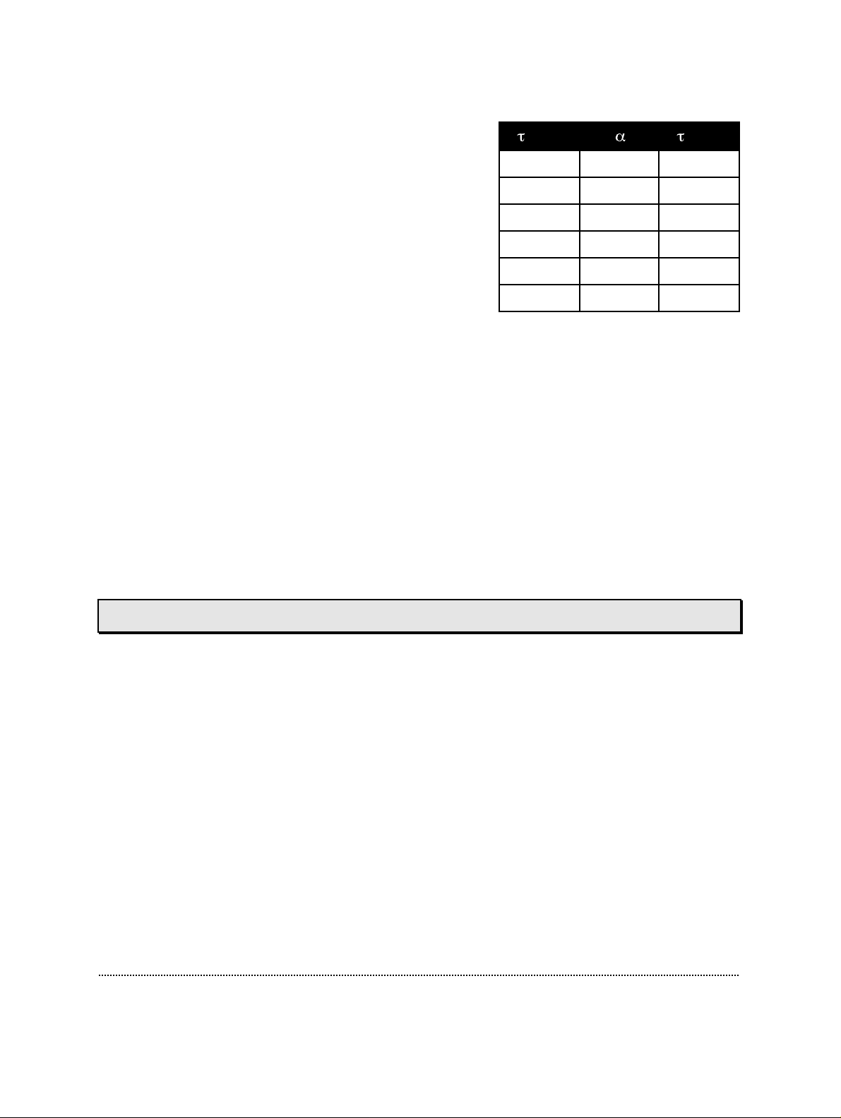
The table gives maximum α values (i.e., %-comp

(µs)

u

(µs)

c

settings) and the resulting τc values in the 2 µs
setting for some values of the uncompensated time

constant τu. At the 10 µs setting, full 90% com­pensation may be used without overshoot for time

90 0.85 13
50 0.80 10
30 0.75 8

constants τu greater than about 1 ms; the 100 µs
setting is appropriate for τu values on the order of
10 ms or longer. In practice, you can estimate τ
from the ratio of the settings of C-slow and R-series.

u

22 0.70 7
13 0.60 5

8 0.50 4

For example, if C-slow is 10 pF and Rs is 10 MΩ, the
time constant is 10 pF · 10 MΩ = 100 µs.

The use of the Rs-compensation circuitry can be summarized as follows: When you
set the capacitance transient cancellation (C-slow, R-series, C-fast, τ-fast) to minimize

the size of the transients when voltage pulses are applied, you have also properly set
them for series resistance compensation. Then you enable R-series and turn up the %-
comp control to the desired value. Any misadjustment of the transient cancellation
will be apparent and can be compensated. The EPC9 makes the procedure very easy:
C-slow and R-series values can be obtained automatically by clicking on Auto C-slow.
Beyond that, the pulse generator provides an option where Auto C-slow is performed
before each command pulse, achieving an accurate update of R-series. The procedure
will be described in more detail later (Chapter 10. Using the Patch Clamp on page 75).

Capacitance Compensation

The EPC9 provides automatic procedures for both fast and slow capacitance
subtraction. In both cases, the ongoing pulse protocols are suspended and short
trains of square-wave pulses are applied (number and amplitude of these pulses are
specified by C-slow Num. Cycles and C-slow Peak Amplitude). The resulting capacitive
transients are averaged, leak-subtracted, and then used to calculate the required
corrections to the components of the compensation network. A detailed description
of the procedures to estimate capacitance is found in Sigworth et. al (1995). The
procedure for C-fast compensation (pipette and stray capacitance) is concerned
mainly with the very initial portion of the transient (the first 10-30 µs), whereas the
procedure for C-slow compensation (whole-cell capacitance) regards a somewhat
later time window. The width of this window is based on an initial guess of what the
time constant of the slow transient might be. Therefore, it is a good idea to set typical
values for C-fast, τ-fast, C-slow and R-series in advance (they may be saved in the
macro for whole-cell recording, for example). This will provide the fitting routine
with reasonable starting values. Alternatively, the Auto procedures can be performed

Compensation Procedures EPC9 Manual 62

alternatingly to arrive at settings for which the remaining transient is minimal.
Settings for C-fast are left at their respective values whenever an Auto C-slow is
performed and vice versa. This way, a combined fit can be obtained by alternatingly
executing Auto C-slow and Auto C-fast. It is better, however, to perform Auto C-fast in
the cell-attached recording configuration and not to touch it any more when
proceeding to whole-cell.

During Auto C-fast and Auto C-slow, certain settings are changed temporarily and
restored upon completion. These are:

• Rs-compensation is switched off

• The gain is set to 0.2, 10 or 50 mV/pA, depending on the gain range in use

• External stimuli are disabled

• Filter 1 is set to 10 or 30 kHz, depending on the required bandwidth

These changes are not displayed on the screen, since they usually are only effective
for fractions of a second. In Cap. Track, however, the changed values are effective for
longer times, since the Auto C-slow procedure is called periodically. It should be kept
in mind that under this condition the parameters on the screen may not represent the
hardware settings.

The relationship between the values of the compensation network (C-slow and R-
series) and those of the pipette-cell assembly (Cm and Rs) is straightforward, if the
membrane conductance is negligible. In this case, perfect compensation will leave no
residual current and C-slow will be equal to Cm. If, however, there is a finite
membrane conductance, then some ambiguity exists, because a three-component
network is being approximated by a two-component compensation network. Details
of the compensation procedure will then determine the residual current (some
filtered version of the command waveform) and Cm is likely to be underestimated.
The Auto C-slow procedure is designed to provide unbiased estimates of the actual
membrane capacitance and series resistance (Sigworth, Neher & Affolter, 1995).

Offset Compensation

In all patch-clamp configurations a number of offsets have to be taken into account.
These include amplifier offsets (± 30 mV), electrode potentials (± 200 mV, depending

on Cl- concentration of pipette and reference electrode), liquid junction potentials,
and potentials of membrane(s) in series with the membrane under study. Some of
these offsets are fixed during an experiment (like amplifier and electrode offsets),
some are variable.

Compensation Procedures EPC9 Manual 63

It is standard practice to take care of the fixed offsets by performing a reference
measurement at the beginning of an experiment. Thereby an adjustable amplifier
offset is set for zero pipette current. Thereafter the command potential of the
amplifier (displayed as V-membrane) will be equal in magnitude to the membrane
potential if no changes in offset potentials occur. The polarity of the command
potential will be that of the membrane for whole-cell and outside-out configurations
but will be inverted in the cell-attached and inside-out configurations. In cell­attached configuration an additional offset is present due to the resting potential of
the cell under study. Liquid-junction potentials may appear or disappear during the
measurement when solution changes are performed or in the case that the pipette
solution is different from the bath solution (Barry & Lynch, 1991; Neher, 1992; Neher,

1995).
Conventionally, these problems are handled by applying the appropriate corrections

and sign inversions during offline analysis. The EPC9 software allows this to be done
at the time of data acquisition, considering the relevant Recording Mode, which may
or may not result in inversion of holding and commanded voltages. In addition, it
offers three features which interact in a way to provide for simple online handling of
offsets, such that V-membrane reads the correct membrane potential (correct both in
polarity and magnitude) at all times. These are:

V0: An adjustable hardware offset-voltage. The actual potential applied to the pipette

is the sum of V-membrane and V0.

Auto-V0: An automatic operation which systematically varies V0 for zero pipette

current. Before doing so, the procedure sets V-membrane to an appropriate value (see
below).

LJ: A software variable which can be set by the user. It represents the sum of all
“variable offsets” applicable at a given time (Offset Sum).

In order for the variable LJ to actually represent the various offsets, and to correct for
these, three conditions have to be met:

• The user has to calculate LJ correctly, according to the rules outlined below.
This value should then be entered in the LJ control.

• A Auto-V0 operation has to be performed at the start of an experiment. The
software will then set V-membrane to -LJ (for Out Out and Whole Cell mode) or
+LJ (for On Cell and In Out modes) at the start of an Auto-V0 operation.

• During experiments, V0 has to be changed in parallel with user-induced
changes in LJ. This is done automatically by Pulse and E9Screen.

Compensation Procedures EPC9 Manual 64

An analysis of the underlying offset problem and justification for the procedures can
be found in Neher (1995).

The rule for calculating the Offset Sum (LJ) is to form the sum of all changes in offsets
which occur between the reference measurement and the test measurement. The
polarity of a given offset voltage should be taken as viewed from the amplifier input
(positive, if positive side of the voltage source is closer to the input). A sign inversion
has to be applied if the offset under consideration disappears.

A procedure how to measure liquid junction potentials is described in Neher (1992).
Ion mobilities for calculation of liquid junction potentials can be found in Barry &
Lynch (1991). The table below lists the values for some typical solutions.

Solution LJ

145 K-glutamate, 8 NaCl, 1 MgCl2, 0.5 ATP, 10 NaOH-HEPES 10 mV
145 KCl, 8 NaCl, 1 MgCl2, 0.5 ATP, 10 NaOH-HEPES 3 mV
60 Cs-citrate, 10 CsCl, 8 NaCl, 1 MgCl2, 0.5 ATP, 20 CsOH-HEPES 12 mV
32 NaCl, 108 Tris-Cl, 2.8 KCl, 2 MgCl2, 1 CaCl2, 10 NaOH-HEPES –3 mV
70 Na2SO4, 70 sorbitol, 2.8 KCl, 2 MgCl2, 1 CaCl2, 10 NaOH-HEPES 6 mV

In each case, a liquid junction potential between the given solution and physiological
saline (main salt: 140 mM NaCl) is listed. Polarity is that of physiological saline with
respect to the given solution (according to the convention of Barry & Lynch).

Note: When applying the above rules for calculating the correction LJ, two sign inversions

of the liquid junction potential are effective for the standard liquid junction potential
correction. First, the liquid junction potential that was present during the reference
measurement disappears during the experiment (after seal formation). Second,
according to Barry & Lynch, the potentials are defined with opposite polarity as
those for patch-clamp experiments (bath vs. electrode instead of electrode vs. bath).
Thus, values in the table can be taken as they are and entered as such in the LJ
control. If however, a liquid junction potential appears during a measurement (e.g.,
during solution changes), then only one sign inversion applies. In that case, the sign
of the value in the table must be inverted before adding it to the “Correction Sum”.

In the following, some specific examples together with explanations will be given. In
all these cases it is assumed that the reference measurement is performed in standard
saline.

Example 1: An outside-out or whole-cell measurement with normal saline in the
pipette. In this case, LJ should be set to zero. This is one of the few measurements
which do not require any correction. It is quite unphysiological, however.

Compensation Procedures EPC9 Manual 65

Example 2: An outside-out or whole-cell measurement with KCl-based internal
solution in the pipette. LJ should be set to 3 mV (see table) in order to correct for the
disappearance of a liquid junction potential between the KCl containing pipette and
the NaCl-based bath solution.

Example 3: An episode with low-chloride bath solution during the experiment of
example 2. It is assumed that the reference electrode in the bath includes a salt bridge

such that the change in Cl- concentration is not “seen” by the Ag-AgCl--wire.
Nevertheless, a liquid junction potential will develop at the bath/salt-bridge
interface, unless a “bleeding” KCl-bridge is used (see Neher, 1992). Similarly, a
liquid junction potential will develop during local microperfusion. Thus, the
correction during the episode in low-chloride medium will be the sum of this liquid
junction potential and the correction of Example 2 (3 mV). Taking the value for a low

Cl- solution (e.g., sulfate Ringer; see table), we arrive at a value of LJ = 3 + (-6) = -3
mV, which should be set during that part of the experiment.

Note: The sulfate Ringer in this case is -6 mV (the inverse of the value in the table),

because this potential “appears” during the measurement with inverted polarity to the
convention of Barry & Lynch.

Example 4: An outside-out or whole-cell measurement with Cs-citrate-based
internal solution. In this case, LJ should be set to 12 mV (see table above).

Example 5: A cell-attached measurement with sulfate-Ringer in the pipette. Two
corrections apply: 1. the correction for the liquid junction potential during the
reference measurement (6 mV, see table above) and 2. the resting potential of the cell.
We assume the latter to be -60 mV and therefore set LJ to -54 mV. In the cell-attached
mode polarities of the amplifier readout are inverted, thus the amplifier will display
the “physiological” patch potential.

Compensation Procedures EPC9 Manual 66

8. Patch-Clamp Setup

Mounting the Probe

For low-noise recording, the pipette holder must be attached directly to the EPC9
probe. Although the probe amplifier can tolerate the additional capacitance of a
short connecting cable without instability or oscillations, we find that the dielectric
and electrostrictive properties of coaxial cables introduce excessive noise. In typical
setups, the probe is therefore mounted directly on a 3-axis micromanipulator. The
EPC9 probes are supplied with a plastic mounting plate for mounting on a flat
surface. Holes can be drilled through the protruding surfaces for attachment to a
matching plate or other surface. Please remember, that the metal case of the probe
must remain insulated from ground.

Because of the extreme sensitivity of the EPC9, special care must be taken in
grounding all surfaces that will be near the probe input in order to minimize line­frequency interference. Even one millivolt of AC on a nearby surface, which can
easily arise from a ground loop, can result in significant 50 or 60 Hz noise. A high­quality ground is available at the Gnd terminal of the probe; this is internally
connected through the probe's cable directly to the Signal Gnd in the main unit. The
Gnd terminal on the probe is best used for the bath electrode, and perhaps for
grounding nearby objects such as the microscope.

Ground Wires

It is a good idea to run a separate ground wire from the Signal Ground jack on the
main unit to ground large objects such as the table, Faraday cage, etc. It is best to
have the high quality ground wire run parallel to the probe's cable in order to avoid
magnetic pickup and ground loop effects. Besides 50 or 60 Hz magnetic pickup,
there may be some 35 kHz pickup from the magnetic deflection of the computer
monitor. This pickup becomes visible only when the EPC9 filters are set to high
frequencies; it can usually be nulled by changing the orientation or spacing of the
ground wire from the probe cable.

Grounding the Microscope

In most cases, the patch clamp is used in conjunction with a microscope; it and its
stage typically constitute the conducting surfaces nearest the pipette and holder. In a

Patch-Clamp Setup EPC9 Manual 67

well-grounded setup, the microscope can provide most of the shielding. Make sure
there is electrical continuity between the various parts of the microscope, especially
between the microscope frame and the stage and condenser, which are usually the
large parts nearest the pipette. Electrically floating surfaces can act as “antennas”,
picking up line-frequency signals and coupling them to the pipette. Make sure the
lamp housing is also grounded. It is usually not necessary to supply DC power to the
lamp, provided that the cable to the lamp is shielded and that this shield is grounded
at the microscope.

External Shielding

Especially when an unshielded pipette holder is used, some electrostatic shielding of
the experimental setup is necessary to avoid line-frequency pickup from lights and
power lines in the room. Most experimenters use a table-top Faraday cage with a
closable front, and lead all of the cables (e.g., from the microscope lamp, probe,
cooling system, ground lines) through a hole in the cage to an equipment rack
mounted outside. If the pipette holder is somewhat exposed, or if the Faraday cage
has an open front, a small grounded screen placed near the pipette holder may help.

Connections to other Instruments

Depending on the needs of the particular user, the EPC9 software can substitute (to a
great extent) for many analog instruments (e.g., variable filter, oscilloscope, pulse
generator, data storage). However, for test purposes, it is still a good idea to have an
oscilloscope connected to the EPC9. You may connect a PCM/VCR combination or
DAT tape recorder to Current Monitor 1, in order to record single-channel activity
continuously at high bandwidth. Also, it is often convenient to observe the voltage
and current monitor signals at the recorder's outputs, rather than directly from the
patch clamp. In most data recorders, the input signals are passed through to the
outputs, and observing the signals there can increase the experimenter's confidence
that the data are being recorded correctly.

Pipette Holder and Electrode

A shielded version of the pipette holder is available; this holder and a properly
grounded microscope can provide sufficient shielding from 50-60 Hz interference
even without the use of a Faraday cage. The shielded holder, however, introduces
much more random noise than the unshielded one. This random noise arises from
the non-ideal dielectric properties of the plastic in the holder and from thermal
voltage fluctuations in films of aqueous solutions; the metal shield allows more of
this noise to be coupled capacitively into the amplifier input. For single-channel

Patch-Clamp Setup EPC9 Manual 68

recordings, the unshielded holder is strongly recommended. The difference in
background noise level between the two holder types is roughly a factor of two.

The unshielded holder is made from polycarbonate, having low dielectric loss. If you
make your own holder, you should give some thought to the choice of materials. The
insulating parts of the holder should be of a low-loss material, and should have a
hydrophobic surface to prevent the formation of conducting water films.
Polycarbonate fulfills these criteria better than any material we have tried. You can
test the noise level of a holder by mounting it (with the electrode wire installed, but
dry) on the probe input, and measuring the noise using the Noise Test facility. The
probe should be in a shielded enclosure, so that no line-frequency pickup is visible
on an oscilloscope connected to the current monitor output at a bandwidth of 3 kHz
or less. A good holder increases the rms noise only by about 10%, e.g., from 95 to 105
fA. Noise sources are discussed in more detail later (Chapter 10. Using the Patch
Clamp on page 75).

The pipette electrode is simply a thin silver wire that is soldered onto the pin that
plugs into the probe's BNC connector. The chloride coating on the wire gets
scratched when exchanging pipettes, but we find that this does not degrade the
stability very much; the wire does need to be re-chlorided occasionally, perhaps once
per month. A wire for the standard electrode holder should be about 4.5 cm long;
after it is chlorided an O-ring is slipped onto it and the wire is inserted into the
holder. Chloriding can be done by passing current (e.g., 1 mA) between the wire and
another silver or platinum wire in a Cl-containing solution (e.g., 100 mM KCl, or
physiological saline). Current is passed in the direction which attracts Cl-ions to the
electrode wire; this produces a gray coating.

Bath Electrode

The main requirements for a bath electrode are that it have a stable electrode
potential and that it does not disturb the composition of the bathing solution. A bare,
chlorided silver wire makes a good bath electrode; however Ag-ions are tolerated
only by som†of cells, such as muscle cells. A good alternative is an electrode
incorporating an agar salt bridge, as illustrated below.

Patch-Clamp Setup EPC9 Manual 69

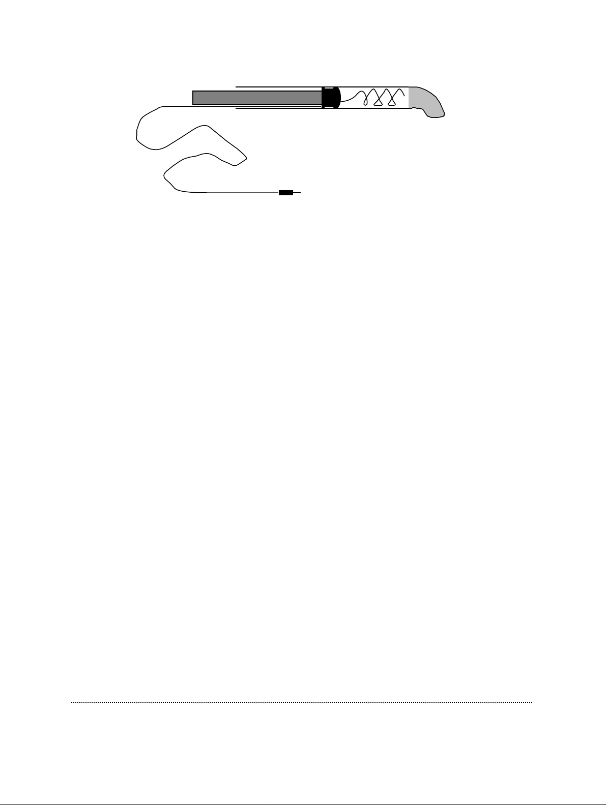
Ag-AgCl wire

to probe GND

agar

The body of the electrode is a 1 ml plastic syringe body that has been heated and
pulled to form a small, bent tip. The electrode proper is a chlorided Ag wire that is
first inserted with the plunger into the fluid-filled body; then hot agar is sucked into
the tip by withdrawing the plunger partially. The filling solution can be a typical
bath solution or something similar, such as 150 mM NaCl. More concentrated salt
solutions are not necessary, and they can leak out, changing the composition of the
bath solution.

Patch-Clamp Setup EPC9 Manual 70

9. Patch-Pipettes

Glass Capillaries

Procedures for fabricating pipettes are presented in some detail in the paper by
Hamill et al. We will summarize the procedure and present some tips that we have
found helpful. The main steps in pipette fabrication are to form a smooth tip on the
pipette (to allow seals to be formed without damaging the cell membrane) and to
coat the pipette with a suitable insulating coating to reduce the background noise.

Pipettes can be made from many different types of glass. Our impression is that
different types of glass work better on different cell types. Glass capillaries are
available from soft (soda glass, flint glass) or hard glasses (borosilicate,
aluminosilicate). Some sources of glass pipettes:

Soft Glass (Supplier) OD

Non-heparinized hematocrit tubing

any scientific supplier

Drummond Microcaps

Drummond Scientific, Bloomall, PA, U.S.A.

Hard Glass (Supplier) OD

Kimax 51

Kimble Products, Vineland, NJ, U.S.A.

Boralec 100

Rochester Scientific, Rochester, NY, U.S.A.

Corning Sealing Glass (#7052, #7040)

Dow Corning, Midland, MI, U.S.A.

GCASS 150-4 (aluminum glass)

A-M Systems, Everett, WA, U.S.A.

1.3 mm

1.4 mm

1.7 mm

1.7 mm

1.6 mm

1.5 mm

Soft-glass pipettes have a lower melting point (800 ˚C vs. 1200 ˚C), are easily
polished, and can be pulled to have a resistance of 1-2 MΩ. They are often used for
whole-cell recording, where series resistance rather than noise is the limiting
criterion. The large dielectric relaxation in soft glass sometimes results in additional
capacitive-transient components that interfere with good capacitance compensation.

Patch-Pipettes EPC9 Manual 71

Hard-glass pipettes often have a narrow shank after pulling and consequently a
higher resistance. Hard glasses tend to have better noise and relaxation properties,
however: the important parameter here is the dielectric loss parameter, which
describes the AC conductivity of the glass. Although the DC conductivity of most
glasses is very low, soft glasses in particular have a conductivity around 1 kHz; that
is sufficiently high to become the major source of thermal noise in a patch-clamp
recording. We find that Kimax glass is a good compromise for whole-cell recording.

Borosilicate and, especially, aluminosilicate glasses (Rae and Levis, 1984) have low
dielectric loss and are desirable for the lowest-noise recordings. They do not
necessarily form the best seals, however; this might be due to evaporation of metal
onto the glass surface during the high-temperature pulling and polishing steps.

Pulling

Pipettes are pulled in two stages: the first to thin the glass to 200-400 µm at the
narrowest point over a 7-10 mm region, and the second to pull the two halves apart,
leaving clean, symmetrical breaks. Both halves can be used. The length of the first
pull and the heat of the second pull are the main determinants of the tip diameter of
the final pipette.

A number of commercial pullers can be used to make pipettes. For reproducibility,
however, a regulated current supply to the heater coil is best. A mechanical stop to
set the length of the first pull is also important for reproducibility.

Coating

The capacitance between the pipette interior and the bath, and also the noise from
dielectric loss in the glass, can be reduced by coating the pipette with an insulating
agent such as Sylgard (Dow Corning Corp., Midland, MI, U.S.A.). Sylgard is pre-cured
by mixing the resin and catalyst oil and allowing it to sit at room temperature for
several hours (or in an oven at 50 ˚C for 20 min) until it begins to thicken. It can then
be stored at -18 ˚C for many weeks until use. The Sylgard is applied around the lower
few mm of the electrode to within 10-20 µm of the tip and then rapidly cured by a
hot-air jet or coil. Coating should be done before the final heat-polishing of the
pipette, so that the heat can evaporate or burn off any residue left from the coating
process.

Patch-Pipettes EPC9 Manual 72

Heat Polishing

Heat polishing is used to smooth the edges of the pipette tip and remove any
contaminants left on the tip from coating. It is done in a microforge or similar setup
in which the pipette tip can be observed at a magnification of 400-800x. The heat
source is typically a platinum or platinum-iridium wire; to avoid metal evaporation
onto the pipette, the filament is coated with glass at the point where the pipette will
approach it. To produce a steep temperature gradient near the filament (which helps
make the pipette tip sharply convergent), an airstream can be directed at the
filament. The amount of current to pass through the filament must be determined
empirically for each type of glass, but a good place to start is with sufficient current
to get the filament barely glowing. The typical practice is to turn on the filament
current and move the filament toward the pipette (which, being stationary, should
remain in focus). Since the opening in the pipette tip is usually at the limit of
resolution of viewing, you might not see the change in shape at the tip, but instead
only a darkening of the tip. You can tell whether you have melted the tip closed, and
also get an idea of the tip diameter, by blowing air bubbles in methanol with air
pressure supplied by a small syringe.

Use of Pipettes

Pipettes should be used within 2-3 hours after fabrication, even if stored in a covered
container; small dust particles from the air stick readily to the glass and can prevent
sealing. However, with some easy-sealing cells we have made the experience that
pipettes may even be used the next day. It is very important to filter the filling
solutions (e.g., using a 0.2 µm syringe filter). Pipettes can be filled by sucking up a
small amount of solution through the tip. This can be done by capillary force (simply
dipping the tip for a few seconds in a beaker containing the pipette solution), or by
applying negative pressure at the back of the pipette (e.g., using a 5 ml syringe).
Thereafter, the pipette is back-filled; the pipette should only be partially filled, just
far enough to make reasonable contact with the electrode wire (the pipette holder is
not filled with solution, but is left dry). Overfilling the pipette has disastrous
consequences for background noise because the solution can spill into the holder,
wetting its internal surfaces with films that introduce thermal noise. Bubbles left in
the pipette from filling can be removed by tapping the side of the pipette.

For low-noise recording, the electrode holder should be cleaned before each
experiment with a methanol flush, followed by drying with a nitrogen jet. Before you
insert a pipette into the holder, it is a good idea to touch a hand to a metal surface of
the setup to discharge any static electricity that you may have picked up. Be sure to
tighten the holder firmly enough that the pipette does not move (on a scale of 1 µm)
when you give suction. Then, when you change pipettes during an experiment,

Patch-Pipettes EPC9 Manual 73

check the noise level of the empty holder using the Noise Test function; if it increases,
solution has probably spilled inside the holder; in this case the holder should be
cleaned again and dried thoroughly.

Patch-Pipettes EPC9 Manual 74

10. Using the Patch Clamp

We give here a brief description of the techniques for establishing a seal and
recording from a membrane patch or from an entire small cell.

Forming a Seal

Initial Setup

The object is to apply voltage pulses to the pipette and observe the Current Monitor
signal on an oscilloscope to monitor the pipette resistance. A convenient way to set
the desired adjustments of the amplifier is by activating the Set-Up mode. The
approach to the cell membrane and the formation of a giga-seal cause the resistance
to increase, reducing the currents. A convenient pulse amplitude is 2 mV, which can
be obtained from the built-in pulse generator. The 2 mV pulses will cause 1 nA to
flow in a 2 MΩ pipette.

For observation of the current pulses, it is convenient to pick a Gain setting and
oscilloscope sensitivity such that the current through the open pipette is reasonably
sized. Other recommended settings are also preset in the Set-Up mode: Voltage Clamp
and V-membrane = 0; Filter 1 is set to 10 kHz and Filter 2 to 3 kHz, Rs-comp to Off, C­slow Range to Off and Stimulus Rise Time to 20 µs. Before the pipette is inserted into the
bath, the current trace should be flat, except for very small capacitive pulses due to
the stray capacitance of the pipette and holder.

Entering the Bath

The surface of the solution is relatively “dirty”, even if (as we strongly recommend)
you aspirate some solution from the surface to suck off dust and contaminants. For
this reason it is important to apply a small amount of positive pressure to the pipette
before you move its tip into the bath, and also to avoid going through the air-water
interface more than once before forming a seal. When you do move the pipette tip
into the bath, the current trace may go off-scale (check clipping); in that case, click on
the Auto-V0 button or reduce the gain until the trace reappears. From the size of the
current response to the test pulses, the pipette resistance can be calculated (the
pipette resistance is displayed in the EPC9 window as R-membrane). If there should
be no change in the trace upon entering the bath, check for an open circuit, for

Using the Patch Clamp EPC9 Manual 75

example: 1. a bubble in the pipette; 2. faulty connection to the probe input; 3. bath
electrode not connected.

There is invariably a small offset potential between the pipette and bath electrodes.
The V0 control is designed to provide a bucking potential to cancel this offset. With
the pipette in the bath, select the Auto-V0 button.

Forming a Gigaseal

When the pipette is pushed against a cell, the current pulses will become slightly
smaller to reflect the increasing seal resistance; when the positive pressure is
released, the resistance usually increases further. Some cell types require more
“push” from the pipette than others, but an increase in resistance of 1.5 (i.e., a
reduction in the current pulses by this factor) is typical.

Application of gentle suction should increase the resistance further, and result
(sometimes gradually, over maybe 30 s; sometimes suddenly) in the formation of a
gigaseal, which is characterized by the current trace becoming essentially flat again
(hyperpolarizing the pipette to -40 to -60 mV often helps to speed the seal
formation). To verify gigaseal formation, increase the Gain to perhaps 50 mV/pA; the
trace should still appear essentially flat except for capacitive spikes at the start and
end of the voltage pulse.

Cell-Attached Recording

You can now use the On Cell mode, which will automatically adjust C-fast and τ-fast
controls to minimize the size of these spikes (some improvement can sometimes be
obtained by manual adjustment). Transient cancellation will be essential if you will
be giving voltage pulses in your experiment. It is a good idea to start out with V-
membrane set to zero, as we specified above; an alternative is to start with V-membrane
set to the holding potential you desire (e.g., -70 mV). If no voltage jumps are
required, turn the stimulus off to avoid introducing artifacts. If voltage jumps are to
be applied, switch the Gain and Filters to the values you will be using (the settings
may be programmed under On Cell).

Be sure to use Gain settings of 50 mV/pA or above for lower noise in single-channel
recordings. Keep the Filter 1 switch set at 10 kHz unless you actually will need the
full 60 kHz bandwidth for some reason; otherwise you might drive the current
monitor output or your recorder's input amplifiers into saturation with the very
large amount of high-frequency noise. Should you use the full bandwidth, you
should avoid gain settings above 100 mV/pA for the same reason.

Using the Patch Clamp EPC9 Manual 76

If you are applying voltage pulses to the patch membrane, you probably will want to
subtract control traces from the traces containing the channels of interest in order to
remove the capacitive transients. Nevertheless, it is important to try to cancel the
capacitive transients as well as you can in order to avoid saturating any amplifiers,
the recording medium or the AD converter. It is a good idea to set the C-fast and τ-
fast controls while you observe the signal without any filtering beyond the internal
10 kHz filter. Then, during the recording, watch to see if the Clipping light blinks.
When it does, it means that internal amplifiers in the EPC9 are about to saturate,
and/or that the Current Monitor output voltage is going above 13 V peak, on the
peaks of the transients, and you should readjust the transient cancellation controls.
Otherwise, it is likely that the recording will be non-linear and subtraction will not
work correctly.

The fast transient cancellation is not sufficient to cancel all of the capacitive
transients in a patch recording. This is partly because the pipette capacitance is
distributed along the length of the pipette; therefore, each element of capacitance has
a different amount of resistance in series with it, so that a single value of τ-fast will
not provide perfect cancellation. The time course of the transients also reflects
dielectric relaxation in the plastic of the pipette holder and in the pipette glass. These
relaxations are not simple exponentials, but occur on time scales of about 1 ms. If
you use pipette glass with low dielectric loss (e.g., aluminosilicate glass) or if you are
careful to coat the pipette with a thick coating and near to the tip, the relaxations will
be smaller. You can cancel part of these slow relaxations by using the C-slow controls,
with the C-slow Range set to 3 pF.

Note: For cell-attached or inside-out patch configuration, positive pipette voltages

correspond to a hyperpolarization of the patch membrane, and inward membrane
currents appear as positive signals at the Current Monitor outputs. The E9Screen and
Pulse programs compensate for this by inverting digital stimulus and sampled values
in these recording configurations such that the stimulation protocols, holding
voltages, and displays of current records in the oscilloscope all follow the standard
electrophysiological convention. In this convention, outward currents are positive
and positive voltages are depolarized. However, the analog current and voltage
monitor outputs are not inverted in these recording modes.

Whole-Cell Recording

Breaking the Patch

After a gigaseal is formed, the patch membrane can be broken by additional suction
or, in some cells, by high voltage pulses (600-800 mV, see Zap function). Electrical
access to the cell's interior is indicated by a sudden increase in the capacitive
transients from the test pulse and, depending on the cell's input resistance, a shift in

Using the Patch Clamp EPC9 Manual 77

the current level. Additional suction sometimes lowers the access resistance, causing
the capacitive transients to become larger in amplitude but shorter. Low values of
the access (series) resistance are desirable and, when Rs-compensation is in use, it is

important that the resistance be stable as well. A high level of Ca2+ buffering
capacity in the pipette solution (e.g., with 10 mM EGTA) helps prevent spontaneous
increases in the access resistance due to partial resealing of the patch membrane.

Capacitive Transient Cancellation

If the fast capacitance cancellation was adjusted (as described above) before breaking
the patch, then all of the additional capacitance transient will be due to the cell
capacitance. Cancelling this transient using the C-slow and R-series controls will then
give estimates of the membrane capacitance and the series resistance. The easiest
way of cancellation is provided by the Auto C-slow function which may be activated
by selecting the Auto button or the Whole Cell mode (if included in the macro
function). In cases where the C-slow transient has a short time constant (100 µs or
smaller) , some improvement of the overall compensation may be achieved by
alternating cycles of Auto C-fast and Auto C-slow (if this doesn't work satisfactorily
you may fine-tune the compensation controls manually). After an iteration or two, it
should be possible to reduce the transient to only a few percent of its original
amplitude. However, if the cell has an unfavorable shape (for example, a long
cylindrical cell or one with long processes), the cell capacitance transient will not be a
single exponential, and the cancellation will not be as complete.

Series Resistance Compensation

Series resistance (Rs) compensation is important when the membrane capacitance is
large or when the ionic currents are large enough to introduce voltage errors. To use

Rs-compensation, you first adjust the transient-cancellation controls (including C-fast
and τ-fast if necessary) to provide the best cancellation. Then you select Rs-comp by

turning up the %-comp control to provide the desired degree of compensation.

Note: The “R-series” control determines (along with the “%-comp” control) the amount of
positive feedback being applied for compensation. It should be adjusted with some care, since
too high a setting causes overcompensation (the EPC9 will think that Rs is larger than it is);

this can cause oscillation and possible damage to the cell under observation.

How you should set the Rs-compensation controls depends on the approximate
value of the uncompensated membrane-charging time constant τu, which you can
calculate as the product of the C-slow and R-series settings (for example, suppose C-

slow is 20 pF and R-series is 10 MΩ; τu is then 20 pF · 10 MΩ = 200 µs). If τu is smaller
than about 500 µs, you should use the 2 µs setting of the Rs-compensation switch to

Using the Patch Clamp EPC9 Manual 78

provide the necessary rapid compensation; however, the slower settings will provide
compensation that is less prone to high-frequency oscillations from misadjustment of
the controls. How much compensation you can apply is also determined by tu. If τ

is larger than about 100 µs, you can use any degree up to the maximum of 90%
compensation without serious overshoot or ringing in the voltage-clamp response.
For smaller values of τu, the %-comp setting should be kept below the point where

ringing appears in the current trace.
As in the case of patch recording, there is rarely need to use the full bandwidth of the

Filter 1 in whole-cell recording. This is because typical membrane charging time
constants (even after Rs-compensation) are considerably longer than 16 µs, which is

the time constant corresponding to a 10 kHz bandwidth. Thus, the current monitor
signal is expected to contain no useful information beyond this bandwidth.

In whole-cell recording, the voltage and current monitor signals follow the usual
convention, with outward currents being positive. This is because the pipette has
electrical access to the cell interior.

Current-Clamp Recording

u

To switch from voltage-clamp to current-clamp recording, just select the Current
Clamp mode. This provides a recording of the cell membrane potential, which can be
monitored at the V-mon output of the EPC9.

When you switch to the Current Clamp mode, the following things happen inside the
EPC9 main unit: The current monitor circuitry is forced into the intermediate Gain
Range (if it was not before), I-membrane is set to a value that will keep the membrane
voltage constant, internal stimulation is stopped, the 10 kHz Bessel characteristic for
Filter 1 is selected, C-slow Ranges is set to Off, and the value of C-fast is reduced by 0.5
pF to avoid oscillations. Rs-compensation will now act as a “bridge balance”. For the

user, these changes are of little consequence and are mainly designed to make
current-clamp recording simple and reliable. The holding current will be displayed
in the original V-membrane display (now converted to I-membrane) and the membrane
potential is shown in the V-mon display of E9Screen. In Pulse, the I-mon display is
converted to V-mon.

Once you have switched to Current Clamp, you can use I-membrane to set a holding
current, and you can apply stimulus pulses via Stim. In. The rule for the scaling of
current stimuli is easy to remember: Any combination of applied stimulus and Stim.
Scale settings that would provide 1 mV of stimulus in the Voltage Clamp mode
provides 1 pA of stimulus in the Current Clamp mode.

Using the Patch Clamp EPC9 Manual 79

11. Low-Noise Recording

The EPC9 amplifier has a particularly low background noise level. The noise level is
in fact low enough that in most experimental situations it can be neglected in view of
other background noise sources that make larger contributions to the total. As we
consider these other sources, first let us make it clear that in this section we are
concerned with random noise, which is fundamentally due to the thermal motion of
electrons and ions; we assume that any user who is interested in low-noise recording
has shielded and grounded his setup sufficiently well to take care of any
synchronous noise due to line-frequency pickup, computer power supplies, TV
cameras, etc. Synchronous noise can be readily identified as stationary features on an
oscilloscope trace when the oscilloscope is triggered by the appropriate signal
source, for example, line-frequency triggering. Grounding and shielding is discussed
in Chapter 10. Using the Patch Clamp on page 75.

The Noise feature of the EPC9 makes it easy for the user to identify important noise
sources. When the Noise button is selected, the I-mon display shows the rms noise
current present in the Current Monitor signal in the frequency band selected by Filter
2 (3 kHz is recommended). For noise measurements, the standard setting of the Gain
control is 50 mV/pA. With the probe placed in a shielded enclosure and with
nothing connected to the input, the Noise reading is usually 80-100 fA. If you get a
reading higher than this, try varying the C-fast control. If you have a noisy stimulus
source connected to Stim. In, the induced current noise will vary with C-fast, with a
minimum occurring with the control set to 1-2 pF, i.e., for best cancellation.

Starting from the intrinsic noise reading of 80-100 fA, one observes increments in the
noise level when the holder and pipette are installed and when an actual recording is
made. By analyzing these increments, you can see where there is the most room for
improvement in your technique. Under the best conditions (i.e., with a clean holder,
an aluminosilicate pipette, etc.), we have observed the noise reading increase to
about 130 fA when the holder and pipette are present, and 160 fA when the pipette
tip is in the bath, sealed on a cell. These are rms current values, which means that
they are equal to the standard deviation of the fluctuating current.

Since the noise sources in the patch clamp amplifier, pipette holder, pipette and
patch membrane are statistically independent, their contributions to the total noise
do not add linearly; instead, their variances (the squares of the standard deviations)
add. This means that the rms reading on the EPC9's display represents the square
root of the sum of the squares of the rms currents from each source. Taking this into
account, one can calculate the relative contributions from the amplifier, pipette

Low-Noise Recording EPC9 Manual 80

holder, and the combination of pipette immersion and patch noise. The table below
shows the relative contributions calculated in this way for the “optimum” situation
just described.

The contributions to the variance

Noise Source Contribution rms Current

from the three sources are seen to
be comparable in size, and impro­vements in the amplifier noise
level will not help very much,

Amplifier 35 % 95 fA

Holder 21 % 73 fA

Pipette + Patch 44 % 105 fA

unless corresponding improvements are made in the other noise sources. As it is,
rms noise values as low as those quoted here are obtained only with considerable
care. Some of the important considerations are outlined below.

As we mentioned in Chapter 8. Patch-Clamp Setup on page 67, the unshielded holder
is greatly superior to the shielded one for low background noise. For low noise, the
holder must be made from a low-loss, hydrophobic plastic; polycarbonate is one of
the best, and plexiglas one of the worst materials. (For our purposes, low-loss
materials are those that show little dielectric relaxation in the frequency range of a
few kHz. Dielectric relaxation involves the reorientation of dipoles within the
material; since any dipoles will be in thermal motion, thermal reorientations in this
frequency range will result in current fluctuations coupled capacitively into the
pipette.)

It is very important that the pipette holder be kept clean and dry. Noise can be
coupled into the pipette from the thermal motion of ions in films of aqueous
solution, especially on the inside of the pipette. A good practice for low-noise work,
is to connect a valve to the pipette-suction line, and arrange for dry air or nitrogen to
flow into the suction line during the time while you change pipettes. This will dry
out any such aqueous films and keep the noise level low.

Films of aqueous solutions and dielectric relaxation are also serious problems with
pipette glass. Coating with Sylgard helps because it is hydrophobic and because it
has good dielectric properties. Also, its thickness helps to reduce the capacitance
between the pipette interior and the bath. This is mainly important because it
reduces the coupling of the glass's dielectric noise into the pipette interior. Clearly,
making thicker coatings (especially in the tip region) and coating closer to the tip will
reduce the pipette noise. The best glass type we know of is aluminosilicate; this glass
requires fairly high temperatures in pulling, and does not necessarily give the best
gigaseals; but its dielectric relaxation appears to be about a order of magnitude
smaller than soft glass.

Some improvement is probably to be gained by taking steps to prevent formation of
aqueous films on the back end of the pipette. It is a good idea to wipe the outside of

Low-Noise Recording EPC9 Manual 81

the pipette to remove any spilled solution, fingerprints, etc. before inserting it into
the holder. It might also help to treat the inside of the pipette to prevent the
formation of a film, for example, by shooting some dimethyl-dichlorosilane vapor
(caution: nasty stuff!) into the back of the pipette before or after filling it.

Lower noise is obtained by immersing the pipette a shorter distance into the bath:
this reduces the coupling of noise currents arising in the pipette glass. A significant
amount of noise seems to arise in the sealed membrane itself and is probably lower
in higher-resistance seals. This noise is generally more than one would calculate
from the resistance of the gigaseal.

The usual goal of low-noise recording is better time resolution: if the noise level is
lower, you can use a wider filter bandwidth to observe single-channel events of a
given amplitude. Judicious use of filtering can improve the time resolution of your
analysis. For example, if you are using the 50%-threshold-crossing analysis technique
to analyze channel open and closed times, the best filter bandwidth is the one that
makes the rms background noise about 1/10 of the channel amplitude. Since one
rarely wants to go through the process of choosing the optimum bandwidth during
an experiment, the best procedure is to record the data at a wide bandwidth and
perform any necessary filtering (analog or digital) later, during analysis of the data.

In typical voltage-clamp, whole-cell recordings the predominant noise source arises
from the combination of the access resistance Rs and the cell membrane capacitance

Cm. Above 1 kHz or so, the current variance from this source increases with this
resistance and capacitance as

2

= Rs C

m

so that it is clearly desirable to keep Rs as small as possible, and, even more
important, to select small cells, if one is interested in low noise. See the chapter by

Marty and Neher (1983) for a more complete description of this and other fine points
of whole-cell recording.

Low-Noise Recording EPC9 Manual 82

Appendix I: Controlling E9SCREEN

Communication between E9Screen and other Programs

E9Screen has two functions which enable a second acquisition program to share the
AD/DA-board. This allows the E9Screen to control the EPC9, while the second program
can use the AD/DA-board for acquisition:

1. E9Screen uses the two functions in the drivers of the AD/DA-board to reserve and
release the AD/DA-board for exclusive use.

2. E9Screen writes a file containing gain and holding potential applied to the EPC9,
and the user program can extract those information from it.

Reserving the AD/DA-board for exclusive use

E9Screen reserves the AD/DA-board for exclusive use, while it performs acquisition.
E9Screen can release the AD/DA-board, when it stops acquiring. This occurs when the
user switches to another application and the option "Enable Background" in the EPC9
drop-down menu is de-selected. E9Screen then resumes acquisition, when the user
switches back and the AD/DA-board driver is not reserved by another process. Thus,
both programs can use the AD/DA-board at well defined times. Please, read in the ITC­16 driver manual ("Driver.pdf") the description of the functions ITC16_Reserve and
ITC16_Release:

• E9Screen calls ITC16_Release, when it is switched to the background and option
"Enable Background" is de-selected.

• E9Screen calls ITC16_Reserve, when it is switched back to the foreground. E9Screen
will continue to call ITC16_Reserve until the function messages that the AD/DA­board has been released by the other application. Only then E9Screen will resume
acquisition.

The “EPC9out.EPC” file

E9Screen writes the file “EPC9out.EPC” in the “E9Screen” folder every time when
switching from E9Screen to another application. This feature can be used by other
acquisition programs to obtain the gain and holding potential applied to the EPC9. The
information in this file is as follows:

Controlling E9Screen EPC9 Installation 83

• In voltage clamp mode (VC-mode):

VHOLD: -0.080; IGAIN: 1.0000E+09
0 [V] 1.0000E+01
1 [-] 1.0000E+00
2 [-] 1.0000E+00
3 [-] 1.0000E+00
4 [-] 1.0000E+00
5 [-] 1.0000E+00
6 [A] 1.0000E+09
7 [A] 1.0000E+09

• In current clamp mode (CC-mode):

IHOLD: 1.0000E-10; IGAIN: 1.0000E+09
0 [V] 1.0000E+01
1 [-] 1.0000E+00
2 [-] 1.0000E+00
3 [-] 1.0000E+00
4 [-] 1.0000E+00
5 [-] 1.0000E+00
6 [A] 1.0000E+09
7 [A] 1.0000E+09

The meaning of the parameters in the first text line are:

• The first character (“V” in VHOLD and “I” in IHOLD, respectively) indicate the
amplifier mode (voltage and current clamp).

• VHOLD gives the applied holding potential in volts. IHOLD gives the applied
holding current in amperes.

• IGAIN gives the amplifier gain in ohms, i.e. V/A. To compute the real current from
a measured voltage, divide it by this value.

The meaning of the parameters in the following lines are:

• The first number is the index of the described AD-channel.

• The letter in the square brackets gives the logical unit of that channel, i.e., "V" for
the voltage monitor, and "A" for the current monitors. A hyphen marks AD­channels without a logical EPC9-function.

• The last number in the line is the gain of that AD-channel. You can derive the
voltage acquired from that AD-channel by the given number to get the correct
value, e.g. the control voltage and the pipette current.

Notes: The line marked "[V]" gives the value of the "Voltage Monitor" BNC-connector

on the EPC9 front panel.
The lines marked "[A]" give the values of the "Current Monitor" BNC­connectors on the EPC9 front panel.

Make sure that the option Enable Background is de-selected, when you want to acquire
data with the EPC9 acquisition board. When E9Screen is in the background, the AD­channel assignments are as follows:

• AD-6 is the I-mon 2 input, i.e., the current input after filter 1 and filter 2.

Controlling E9Screen EPC9 Installation 84

• AD-7 is the I-mon 1 input, i.e., the current input after filter 1.

To read V-mon, one has to connect the corresponding V-mon output of the EPC9 to any
suitable AD-input channel (but not 6 or 7). The user can now switch between two
programs. In this configuration, one can use the user program for data acquisition and
processing, while E9Screen is used to control the EPC9 settings, such as gain and
compensations. The holding potential is best set in E9Screen. If the holding potential
should be set from the user program, one has to control DA-3, which directly applies the
voltage to the EPC9 (scaling is 0.1, i.e., an input of 100 mV will translate to 10 mV).
Alternatively, voltages can be applied to the EPC9 by setting DA-0, DA-1, or DA-2, and
connecting that DAC to the external stimulus input of the EPC9. In this case, activate the
External Stimulus Input option in E9Screen, i.e., setting an appropriate external stimulus
scaling factor.

Controlling the EPC9 from another Program

Sending Commands to E9Screen

E9Screen can be controlled from another program by a simple “batch file control”
protocol. This “batch file control” protocol is simple, fast, and platform independent. The
new control protocol allows to control the EPC9 over a network, even one with different
platforms, such as Windows, Macintosh, Unix, OS/2, or workstations. Thus, it is now
possible to control the EPC9 from computers running a multitasking operating system
which can create and read shared files (e.g., Windows 95, Windows NT, MacOS, etc.).

Controlling E9Screen from another program is possible by communicating via two
ASCII-files. The user writes the commands to one file (the “command” file) and E9Screen
communicates back by writing to a second file (the “response” file). The user program
has write permission (plus sharing permission) on the “command” file it will write to.
E9Screen will access that file with read and shared permission only. The reverse is used
on the second file, the “response” file: E9Screen will have write and sharing permission,
and the user program read permission only (plus sharing permission, of course).

The first line in the “command” file must contain one positive number (as ASCII, e.g.,
“+1234”). This “command index” is interpreted by E9Screen as follows:

• If this number is zero or negative, E9Screen does not execute the commands in the
“command” file.

• If the number is larger than zero, E9Screen will execute the instructions
immediately. E9Screen will write that number to the “response” file to flag
execution once all commands have been executed.

• To prevent E9Screen to execute the instructions more than once, E9Screen will not
execute any further commands until the “command index” value is changed by the
user program.

Controlling E9Screen EPC9 Installation 85

• Every command plus the required parameters must be in one text line, i.e.,
terminated by a “CR” character code (any following linefeed character will be
ignored).

• E9Screen writes the responses to the “response” file. In the first line of that file,
E9Screen writes the “command index”. The following lines will contain the
responses, if any, one response per line.

• The name of the “command” file must be “E9Batch.In”, the one of the “response”
file “E9Batch.Out”. Both files will be inside the default folder of E9Screen, usually
the folder “E9Screen”.

Thus, communication would proceed as follows:

➊ The user program is started first:

It has to create a file in the “E9Screen” folder named “E9Batch.In”. It has to keep
this file open with “write” and “shared” access permission.

➋ Then E9Screen is started:

Enable the “Enable Batch Control” option. E9Screen will open the file
“E9Batch.In” with “read” and “shared” access permission. Also, E9Screen will
now create the "E9Batch.Out" file with “write” and “shared” access permission.

➌ Now, E9Screen will immediately execute the commands in the command file,

provided that the “command index” is larger than zero. E9Screen writes the
“command index” and eventually any error and requested answer to the
“response” file.

➍ Next, the user switches back to the user program.
➎ Any time the user program writes to the “command” file, E9Screen will scan the

command file and execute the commands, if the “command index” changed.
Windows 95 and Windows NT: On computers running Windows 95 or Windows

NT, E9Screen will immediately execute the commands.
Macintosh: On computers running MacOS, E9Screen will immediately execute

the commands, if it is the front application. If E9Screen is not the front
application, then E9Screen will get active when the front application calls the
“Toolbox” routine “GetNextEvent” or “WaitNextEvent”.

➏ The user program can now read the “response” file. The first line should mirror

the “command index”. Subsequent text lines may contain responses and error
messages (see list below). There are the following possibilities:

- There is no further line in the response file. This means, that no error occurred
during execution and that no response was requested.

- There is additional text in the file. The user can easily recognize error
messages, because the first character in an error message is a lower case letter.
All other responses start with an upper case letter.

Controlling E9Screen EPC9 Installation 86

➐ When the user program wants to issue new commands, it writes a new

“command index” and the new commands to the “command” file, then
continues with step 5.

Here is an example of such a command file:

1. line: "1234"

2. line: "SetVHold -0.080"

3. line: "GetCurrentRange"

4. line: "MakeAnError"

And this would be the content of the “response” file:

1. line: "1234"

2. line: "CurrentGain 1.000E+09"

3. line: "unknown"

Error Messages

Errors begin with lower case letters:

'syntax' : parameter missing or misspelled
'range' : parameter is out of allowed range
'unknown': command is unknown
'ioerror': error during an I/O-operation
'unknown error': an unidentified error occurred

Implemented Commands and Messages

Messages send by E9Screen. They do not contain a response string.

Started E9Screen started communication link
Terminated E9Screen terminated communication
InFront E9Screen got the front application
Running E9Screen was switched to the background
(see "Query" command below).
ADReserved E9Screen reserved the AD/DA-board for
exclusive use and resumed acquisition
ADRelease E9Screen released the AD/DA-board and
and stopped acquisition

Operations without parameters. They do not return a response.

AutoCFast
AutoCSlow
AutoGLeak
AutoVpOffset

“Get” operations: They have no parameters and return one parameter. The response
always repeats the command string without the “Get” sub-string.

GetCCFastSpeed
GetCCIHold
GetCCStimScale
GetCFast1
GetCFast2

Controlling E9Screen EPC9 Installation 87

GetCFastError
GetCFastTau
GetClipping
GetCSlow
GetCSlowError
GetCSlowRange
GetCurrentGain get gain in Ohms (i.e., V/A)
GetE9SBoard
GetE9SerialNo
GetF2Butterworth
GetF2Frequency
GetFilter1
GetGLeak
GetGSeries
GetIpipette
GetLastVHold
GetMode
GetRmembrane
GetRsFraction
GetRsMode
GetRsValue
GetStimFilterOn
GetVCStimScale
GetVersion
GetVHold
GetVLiquidJunction
GetVmonitor
GetVpOffset

“Set” operations: They have no or one parameter and do not return a response.

SetAdcChannel integer: 0 to 12 -> FExt, Vmon, Imon1, Imon2,

none, ADC0 .. ADC7
SetCCFastSpeed boolean: 0 or 1
SetCCIHold real: current in Amperes
SetCCRange boolean: 0 or 1
SetCFast2 real: capacitance in Farad
SetCFastTau real: tau in seconds
SetCSlow real: capacitance in Farad
SetCSlowRange integer: 0,1,2,3 -> off,30,100,1000pF range
SetCurrentGain set gain in Ohms (i.e., V/A)
SetE9Board integer: 1,2,3
SetF2Frequency real: bandwidth in Hertz
SetF2Butterworth boolean: 0 or 1
SetFilter1 integer: 0,1,2,3 -> 100,30,10kHz,HQ30kHz
SetGLeak real: in Siemens (i.e., 1/Ohms)
SetGSeries real: in Siemens (i.e., 1/Ohms)
SetLastVHold no parameters
SetMode 0 to 3, corresponding to Test, VC, and CC.
SetRsFraction real: 0.0 to 0.95
SetRsMode integer: 0,1,2,3 -> off,100,10,2 µs
SetRsValue real: in Ohms
SetStimFilterOn boolean: 0 or 1
SetStimScale real: -10.0 to +10.0 (0.0 means off)
SetTestPulse boolean: 0 or 1
SetVHold real: -1.0 to +1.0 Volt
SetVLiquidJunction real: -1.0 to +1.0 Volt minus VHold
SetVpOffset real: -0.2 to +0.2 Volt

Miscellaneous Operations

Controlling E9Screen EPC9 Installation 88

acknowledged (re-synchronize command index)
syntax: "acknowledged"
no parameters
no response

ADRead
syntax: "ADRead AD-channel"
AD-channel: integer 0 to 7
returns a real (read AD-value in Volts)

ADRelease
syntax: "ADRelease"
no parameters
returns string "ADReleased"

ADReserve
syntax: "ADReserve"
no parameters
returns:
if it could reserve the AD-board: string "ADReserved"
otherwise: string "ADReleased"

DAWrite
syntax: "DAWrite AD-channel Volts"
DA-channel: integer, 0 to 3
Volts: real, +/-10.24 volt
no response

ExecMacro
syntax: "ExecMacro MacroIndex"
MacroIndex: integer, 0 to 6
no response

MeasureNoise
syntax: "MeasureNoise"
no parameters
returns a real

Query
syntax: "Query"
no parameters
returns the string "Running"

Reset
syntax: "Reset"
no parameters
no response

Terminate
syntax: "Terminate"
no parameters
returns the string "Terminated"

Key
syntax: "Key ASCII-code Key-Code"

Key-Codes:
2 -> Normal character input

Controlling E9Screen EPC9 Installation 89

cursor keys:
3 -> KeyCursorUp
4 -> KeyCursorDown
5 -> KeyCursorLeft
6 -> KeyCursorRight

numeric keypad:
7 -> 0 (zero) on numeric keypad
8 -> 1 on numeric keypad
9 -> 2 on numeric keypad
10 -> 3 on numeric keypad
11 -> 4 on numeric keypad
12 -> 5 on numeric keypad
13 -> 6 on numeric keypad
14 -> 7 on numeric keypad
15 -> 8 on numeric keypad
16 -> 9 on numeric keypad
17 -> Enter
18 -> minus on numeric keypad
19 -> plus on numeric keypad
20 -> period on numeric keypad
21 -> clear on numeric keypad (above '7')
22 -> '=' on numeric keypad (above '8')
23 -> '/' on numeric keypad (above '9')
24 -> '*' on numeric keypad

function keys (F1 to F15):
24 + function key number, e.g., 25 for F1

key block above cursor keys:
40 -> HOME
41 -> END
42 -> PageUp
43 -> PageDown
44 -> HELP
45 -> Delete Left
46 -> Delete Right

Controlling E9Screen EPC9 Installation 90

Notes to Programmers

If one uses the EPC9 acquisition board to acquire data in a user program, one has to be
very aware that the EPC9 is controlled through its AD/DA-board as well. Thus, every
time E9Screen has to talk to the EPC9, it will unconditionally make use of the AD/DA­board. Yet, when E9Screen is not the front application (Windows programmers call it
"focus") and the "Enable Background" option is not selected, then E9Screen gets active
only when it receives a command through the "batch control" handshaking. Therefore,
the "Enable Background" option in the EPC9 drop-down menu must be off.

One other problem spot is to define when to open the message file. This file is created by
E9Screen. Therefore it cannot and should not be opened before E9Screen is running.
Thus, the user program has to delete any message file it finds upon starting. That file
may still be left around from a previous session. A good option is to create an empty
command file in the directory where E9Screen is located and to wait for the message file
to appear in the E9Screen directory. At that moment one can start E9Screen and enable
the option "Enable Batch Control" in the EPC9 drop-down menu. The message file will
then be created and the user program can now open it for reading and sharing.

The first response E9Screen writes to the message file is "Started". Thereafter the user can
proceed to send commands to E9Screen and read back the response.

It is advisable to write to the command file in an analogous way as it is done in the
example code below. In principle, one should proceed as follows:

1. Write a minus sign ("-") to the first byte of the command file. This prevents E9Screen
from interpreting anything in the file while the user programs writes to it. Please, recall
that some operating systems are multitasking. This means that both programs, E9Screen
as well as the user program, run concurrently. Thus, E9Screen may attempt to read from
the message file while the user program is writing to it!

2. Write the remaining of the first text line. The first text line must be the signature
number. The sample code below writes the negative value of the signature to achieve:

- a negative sign is placed in the first byte of the file;

- the signature value is written; and

- the final, positive signature can be obtained by replacing the negative sign with a

plus ("+").

3. Write to following text lines the required instructions, one instruction per text line.

4. Finally, replace the negative sign in the first byte of the file with a plus ("+"). This will
signal to E9Screen to proceed to read and interpret the command file.

5. Monitor the content of the message file. Do not interpret the content of the message
file, as long as the first byte is a minus sign ("-") or the signature value in the first line is
the one used in writing the last command.

Controlling E9Screen EPC9 Installation 91

6. E9Screen writes responses to the message files in the following situations:

- On starting "batch" processing, it messages "Started".

- Responding to a "Get", "Query", or "Terminate" instruction.

- When an error occurred while scanning the message file.

Controlling E9Screen EPC9 Installation 92

Sample program

The listing below is an excerpt from the program used to test the E9Screen
communication protocol. It demonstrates the functions needed to write an own program
to control the EPC9 through the E9Screen program. The code is written in Modula-2. The
code can be easily understood also by readers familiar with BASIC, PASCAL, C, C++, or
FORTRAN.

MODULE UserCommands;

CONST
CommandName = 'EPC9In.EPC';
MessageName = 'EPC9Out.EPC';

VAR
CommandFile : IOFiles.FileHandleType;
MessageFile : IOFiles.FileHandleType;
Signature : INTEGER;
LastSignature : INTEGER;

PROCEDURE WriteError( Text : ARRAY OF CHAR );
VAR
Work : ARRAY[0..79] OF CHAR;
BEGIN
IOFiles.Message( IOFiles.GetError(), Work );
TermIO.WriteString( Text );
TermIO.WriteString( ' failed: ' );
TermIO.WriteLine( Work );
Alert.Beep;
END WriteError;

PROCEDURE WriteToCommandFile( Text : ARRAY OF CHAR ): BOOLEAN;
VAR
Work : ARRAY[0..79] OF CHAR;
Count : INTEGER;
BEGIN

IF NOT CommandFile.IsOpen THEN RETURN FALSE; END;

IF Text[0] = 0C THEN RETURN TRUE; END;

Work[0] := 0C;
Decode.Integer( - ABS( Signature ), Work, 0 );
Count := Strings.Length( Work );

(* First, we write a negative signature to the first text line.
This prevents to the target E9Screen to read and interpret
the content of this file. We use the actual signature already
now, so that we can just change the sign from negative to
positive by overwriting one character!
*)

IF

Controlling E9Screen EPC9 Installation 93

( NOT IOBytes.SetLength( CommandFile, 0 ) ) OR
( NOT IOText.Write( CommandFile, Count, ADR( Work ) ) )
THEN
WriteError( 'Writing negative signature' );
RETURN FALSE;
END; (* IF *)

Count := Strings.Length( Text );

(* Second, we write the command text to the second (and following)
line.
*)

IF NOT IOText.Write( CommandFile, Count, ADR( Text ) ) THEN
WriteError( 'Writing to command file' );
RETURN FALSE;
END; (* IF *)

(* Third, if the signature should be positive, we now overwrite the
negative sign (i.e., "-") of the signature in the first line with
a plus (i.e., "+"), thus changing the negative signature to positive.
See above for the explanation.
*)

IF Signature >= 0 THEN
Work[0] := '+';
Count := 1;

IF
( NOT IOBytes.SetPosition( CommandFile, IOFiles.FromStart, 0 ) ) OR
( NOT IOBytes.Write( CommandFile, Count, ADR( Work ) ) )
THEN
WriteError( 'Writing positive signature' );
RETURN FALSE;
END; (* IF *)
END; (* IF *)

TermIO.WriteLn;
TermIO.WriteString( 'command : [' );
TermIO.WriteInt( Signature, 0 );
TermIO.WriteString( '] ' );
TermIO.WriteLine( Text );

INC( Signature );

IF Signature < 1 THEN Signature := 1; END;

RETURN TRUE;

END WriteToCommandFile;

PROCEDURE OpenMessageFile(): BOOLEAN;
BEGIN

IF NOT CommandFile.IsOpen THEN RETURN FALSE; END;

IF MessageFile.IsOpen THEN
Alert.String( 'Message file already open! ' );
RETURN FALSE;

Controlling E9Screen EPC9 Installation 94

END; (* IF *)

IF NOT
IOText.Open(
MessageName,
IOFiles.Read + IOFiles.Shared,
MessageFile )
THEN
IF IOFiles.GetError() <> IOFiles.FileNotFound THEN
WriteError( 'Opening message file' );
END; (* IF *)
RETURN FALSE;
END; (* IF *)

LastSignature := -1;

RETURN TRUE;

END OpenMessageFile;

PROCEDURE PollForCommands;
VAR
InputString : ARRAY[0..127] OF CHAR;
NewSignature : INTEGER;
Count : INTEGER;
Dummy : BOOLEAN;

BEGIN

IF NOT CommandFile.IsOpen THEN
RETURN;
END; (* IF *)

IF ( NOT MessageFile.IsOpen ) AND ( NOT OpenMessageFile() ) THEN
RETURN;
END; (* IF *)

(* Read the first text line. If reading fails, or converting to a number
fails, or the resulting number is negative, then the answer from the
target E9Screen is not ready.
*)

NewSignature := -2;
Count := HIGH( InputString );

IF
( NOT IOText.SetPosition( MessageFile, IOFiles.FromStart, 0 ) ) OR
( NOT IOText.Read( MessageFile, Count, ADR( InputString ) ) )
THEN
RETURN;
END; (* IF *)

IF ( InputString[0] = 0C ) OR ( InputString[0] = '-' ) THEN
RETURN;
END; (* IF *)

Count := Encode.Integer( InputString, NewSignature );

IF ( NewSignature < 0 ) OR ( LastSignature = NewSignature ) THEN

Controlling E9Screen EPC9 Installation 95

RETURN;
END; (* IF *)

TermIO.WriteString( 'response: [' );
TermIO.WriteInt( NewSignature, 0 );
TermIO.WriteString( '] ' );

Count := HIGH( InputString );

IF IOText.Read( MessageFile, Count, ADR( InputString ) ) THEN
TermIO.WriteLine( InputString );
ELSE
(*
If the "response" text is empty, then the command has been
sucessfully processed!
*)
TermIO.WriteLine( 'done.' );
END; (* IF *)

LastSignature := NewSignature;

IF ( NewSignature > Signature ) OR ( NewSignature = 0 ) THEN
Signature := NewSignature + 1;
Dummy := WriteToCommandFile( 'acknowledged' );
END; (* IF *)

END PollForCommands;

PROCEDURE Startup(): BOOLEAN;
VAR
Temp : IOFiles.FileNameType;
Path : IOFiles.FileNameType;
BEGIN

IF CommandFile.IsOpen THEN
Alert.String( 'Command file already open! ' );
RETURN FALSE;
END; (* IF *)

Strings.Assign( Temp, 'E9Screen.exe' );
Strings.Clear( Path );

IF NOT
FileSelect.Select(
Temp,
Path,
'*.*',
FileSelect.ExistingFile + FileSelect.ChangeDirectory,
'Select any file in target E9Screen folder:' )
THEN
RETURN FALSE;
END; (* IF *)

Controlling E9Screen EPC9 Installation 96

IF NOT
IOText.Open(
CommandName,
IOFiles.Create + IOFiles.Write + IOFiles.Shared,
CommandFile )
THEN
WriteError( 'Opening command file' );
RETURN FALSE;
END; (* IF *)

Signature := 1;

RETURN TRUE;

END Startup;

PROCEDURE InitModule;
BEGIN
CommandFile.IsOpen := FALSE;
MessageFile.IsOpen := FALSE;
Signature := 1;
LastSignature := -1;
END InitModule;

PROCEDURE Shutdown;
VAR
Dummy : BOOLEAN;
BEGIN
Dummy := WriteToCommandFile( 'Terminate' );
Dummy := IOText.Close( CommandFile );
Dummy := IOText.Close( MessageFile );

InitModule;
END Shutdown;

END UserCommands.

Controlling E9Screen EPC9 Installation 97

Appendix II: Technical Data

Pin number

EPC9

Pin number

EPC9

1

IN-0

2

OUT-14

3

Not connected

4

OUT-15

5

IN-2

6

IN-10

7

IN-3

8

IN-11

9

IN-4

10

IN-12

11

IN-5

12

IN-13

13

IN-6

14

IN-14

15

IN-7

16

IN-9

17

IN-1

18

CLIPPING

19

GND

20

GND

21

GND

22

GND

23

24

STROBE-out

25

OUT-0

26

OUT-8

27

OUT-1

28

OUT-9

29

OUT-2

30

OUT-10

31

OUT-3

32

OUT-11

33

OUT-4

34

OUT-12

35

OUT-5

36

OUT-13

37

OUT-6

38

IN-8

39

OUT-7

40

Not connected

Digital I/O Connector

EPC9

The pin assignment of the 40-pin connector on the EPC9 is:

Not connected

The digital IN and OUT lines carry TTL-compatible signals.

Technical Data EPC9 Manual 98

PIN 1 of the 40-pin connector is labled with a small arrow:

Pin number

EPC9

Pin number

EPC9

1

TRIGGER-0

2

TRIGGER-1

3

TRIGGER-2

4

TRIGGER-3

5

TRIGGER-4

6

TRIGGER-5

7

TRIGGER-6

8

TRIGGER-7

91011121314151617

Ground IN

18

Power IN

19

Ground IN

20

Power IN

21222324252627282930313233343536373839

40

PIN 39

PIN 40

PIN 1

PIN 2

EPC9 Double and Triple

The pin assignment of the 40-pin connector on the EPC9 Double and Triple is:

The TRIGGER OUT 0 to 7 are opto-coupled open collector outputs (max. 1A). One
can use these outputs to control external devices, e.g. solenoid driven valves. One
can also generate TTL signals. Below it is described how to generate both types of

Technical Data EPC9 Manual 99

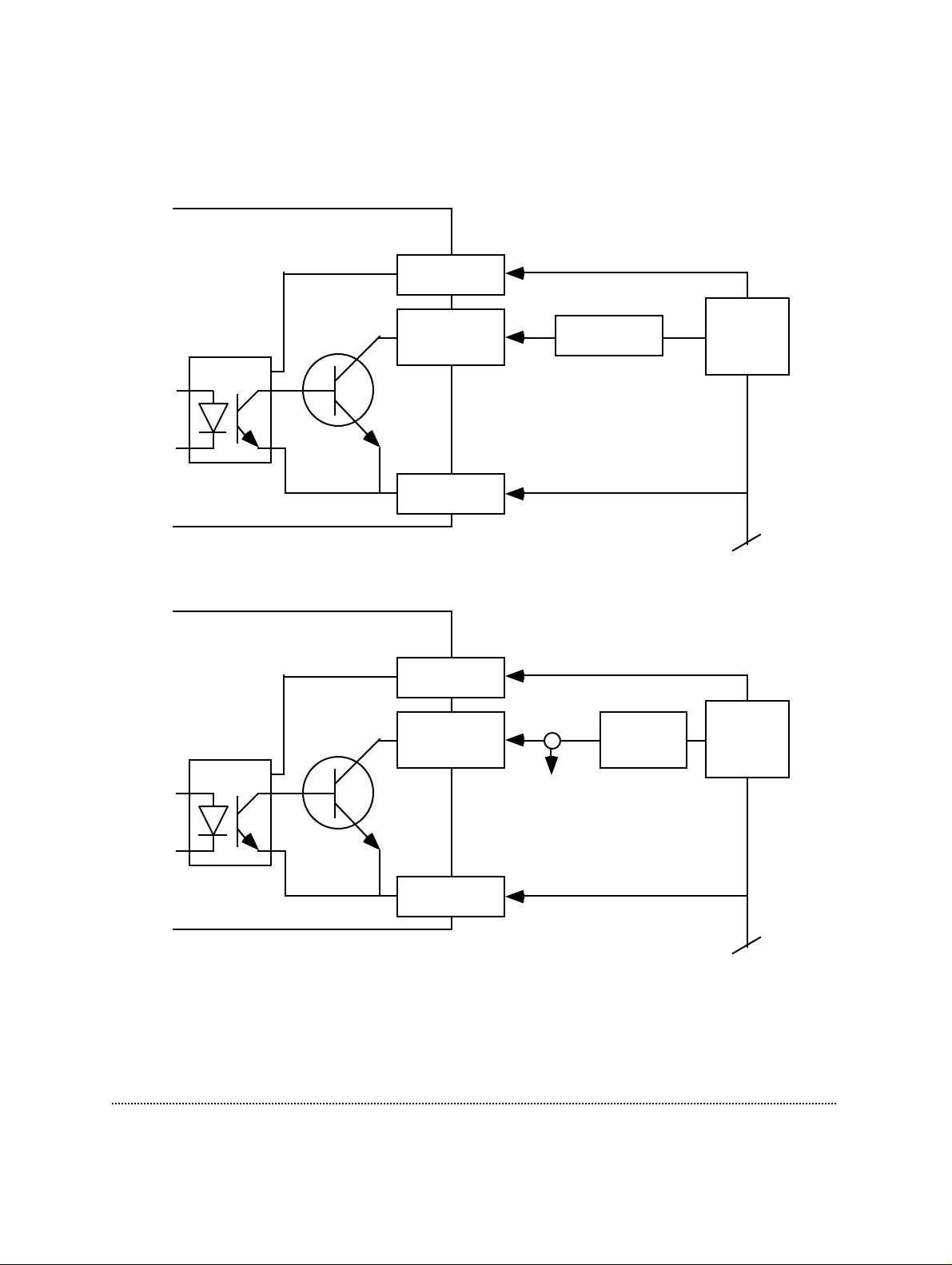
connections. The current drivers can sink up to 1 A current. The maximal power
supply voltage should not exceed 24V.

EPC 9 Double External

Power IN

+5 .. 24V

Power

supply

Ground

OPTO

TRIGGER

OUT

Ground IN

Arrangement for current driven devices

Valve

EPC 9 Double External

Power IN

TRIGGER

OUT

OPTO

Resistor
5 kOhm

Power

supply

TTL

+5V

Ground IN

Ground

Arrangement to generate TTL signals

Technical Data EPC9 Manual 100