

Page 1
OPERATIONAL MANUAL FOR THE HEATH
EDUCATIONAL ANALOG COMPUTER
MODEL EC-1
PREFACE
The purpose of this manual is threefold: first, to present, in elementary form, the fundamental
mathematical theory of analog computers; second, to provide instructions for operation of the
Heath Educational Analog Computer; and third, to show some illustrative examples of problems
which can be solved on the Computer.
This manual is not intended to be exhaustive but rather to be a guide in the operation of the
computer. For this reason frequent references are made to the available literature. Several
excellent books as well as many articles are available. Some of these are listed in the references at
the end of the manual. These should be available to and used by anyone with a serious interest in
analog computers.
3/20/59
Page 2

CONTENTS
Preface ...........................................................................................................1
Introduttion ................................................................................................... 3
Theory ............................................................................................................4
Circuit Description
DC Operational Amplifier .....................................................................13
Amplifier Powe r Supply ........................................................................14
Initial Co ndition Power Supplies .........................................................15
Control Circuit ......................................................................................15
Repetitive Oscillator ..............................................................................15
General Operating Instructions .................................................................16
Basic Mathematical Operations
Addition .................................................................................................17
Multiplication ........................................................................................19
Integration .............................................................................................19
Illustrative Problems
Falling Body ...........................................................................................21
Spring-Mass System .............................................................................24
Simultaneous Algebraic Equations ......................................................26
Proje ctile ................................................................................................27
Bouncing Ball ........................................................................................28
Reference s .......................................................................................................
....................................................................................................... 31
Specifications ..............................................................................................32
Parts List .....................................................................................................34
Page 2
Schematic ....................................................................................................38
Page 3

INTRODUCTION
One of the wonders of the modern Electronic Age is the computer or "Giant Brain", as it is
sometimes called. Actually, the computer is not a "Brain" at all, since it does not think but must
be "told" what to do. It is capable of doing mathematical operations at much greater speed and with
greater accuracy than human beings.
A computer is a machine which performs physical operations that can be described by mathematical operations. In general, computers may be classified as digital or analog. Digital computers
operate by discrete steps, that is, they actually count. Common examples of digital computers are
the abacus, desk calculator, punched-card machine, and the modern electronic digital computer.
The fundamental operations performed by the digital computer are usually addition and
subtraction. Multiplication, for example, is accomplished by repeated additions.
Analog computers operate continuously, that is, they measure. Examples of analog computers are
the slide rule (which measures lengths), the mechanical differential analyzer, the electromechanical analog computer and the all-electronic analog computer. The last three generally
measure electrical voltages or shaft rotations. Physical quantities such as weight, temperature or
area are represented by voltages. Voltage
Arbitrary scale factors are set up to relate the voltages in the computer to the variables in the
problem being solved. For example, 1 volt equals 5 feet or 10 volts equals 1 pound. The name
"analog" comes from the fact that the computer solves by analogy by using physical quantities to
represent numbers.
The fact that the analog computer operates continuously makes it very useful in such operations
as integration; for this reason computers used this way are sometimes known as Differential
Analyzers.
One of the most powerful applications of analog computers is simulation in which physical
properties, not easily varied, are represented by voltages which are easily varied. Thus the "knee
action" of an automobile front wheel suspension can be simulated on an analog computer in which
the weight of the automobile, the constant of the spring, the damping of the shock absorber, the
nature of the road surface, the tire pressure and other conditions can be represented by voltages.
In practice these factors cannot be readily changed, but on the computer any one or all of these
may be varied at will and the results observed as the changes are made.
Analog computers are especially useful in solving dynamic problems in which the motion can be
expressed in the form of a differential equation.
All mathematical operations necessary to the solution of ordinary differential equations can be
built up from addition, multiplication by a constant, and integration. * As will be shown later, the
analog computer can perform these operations and thus is a convenient device for the solution of
differential equations.
The combination of the six basic computer operations will perform any continuous function.
Some of the types of problems which can be solved by these methods are radioactive decay,
chemical reaction, beam oscillation and heat flow. With the addition of crystal diodes and re-lays,
simulation of discontinuous functions is possible. This makes possible solution of problems
involving saturation, backlash, hysteresis, friction, limit stops, vacuum tube characteristics, and
different modes of operation such as sonic vs. subsonic flow.
is the electrical analog of the variable being analyzed.
* Shannon, C. , JOURNAL MATH. AND PHYSICS, Vol. 20, Pages 337-354, 1941.
Page 3
Page 4
With the addition of special devices such as function generator and function multiplier, additional operations may be performed such as multiplication of variables, computation of trigonometric, exponential and logarithmic functions and generation of discontinuous functions. *
THEORY
In order to solve differential equations on an analog computer, it is necessary to have:
1. DC amplifiers (also called operational amplifiers) capable of performing the operation of
a. Integration
b. Addition (or summation)
c. Multiplication by a constant
d. Multiplication by -1(inversion)
2. A means of setting coefficients in a problem. This may be done by means of
a. Potentiometers
b. Changing the ratio of feedback resistance to input resistance.
3. A control system for starting and stopping solution of the problem, as well as resetting the
initial conditions so as to be ready for running a new solution with the same or new
coefficients and initial conditions.
The general procedure in solving a problem is to:
1. Set the machine variables (voltages) to the correct initial conditions.
2. Make the computing elements operative and force the voltages to vary in the manner
prescribed by the differential equations.
3. Observe and/or record the voltage variations, with respect to time, which constitute the
solution of the given problem.
4. Stop the machine and reset for a new run.
The heart of the analog computer is the DC operational amplifier which performs the basic
mathematical operations necessary for the solution of problems.
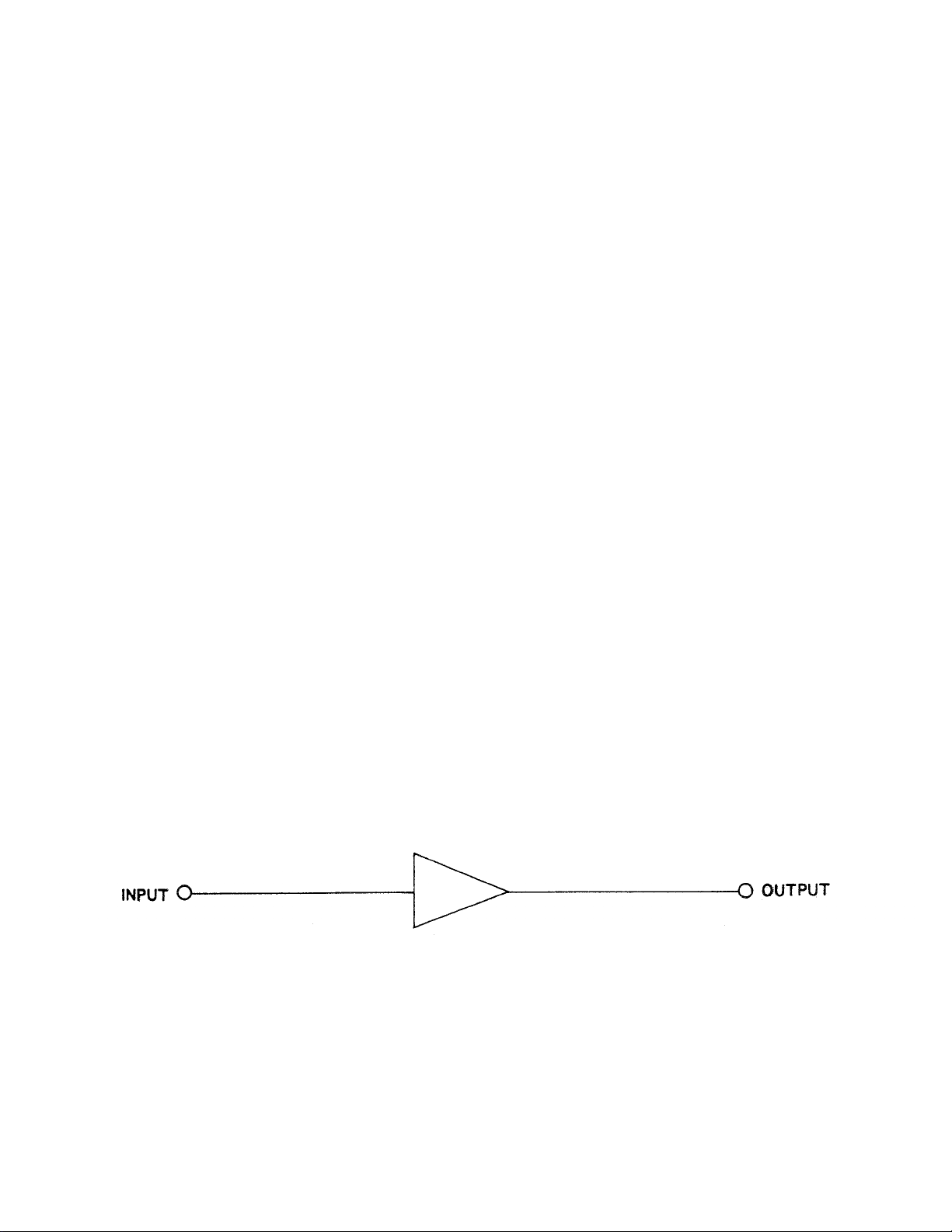
The amplifier used in the analog computer
feedback and is represented by a triangle with the base at the input end and the apex at the output end, as shown in Figure 1.
is a high gain direct-coupled amplifier with negative
Figure 1
AMPLIFIER SYMBOL
* Clarence L. Johnson, ANALOG COMPUTER TECHNIQUES (McGraw-Hill Book Company, Inc.,
New York 1956) Chapter 8, Pages 13 6-164.
Korn and Korn, ELECTRONIC ANALOG COMPUTERS (McGraw-Hill. Book Company, Inc. , New
York 1956) Second Edition, Chapter 6, Pages 251-344.
Page 4
Page 5
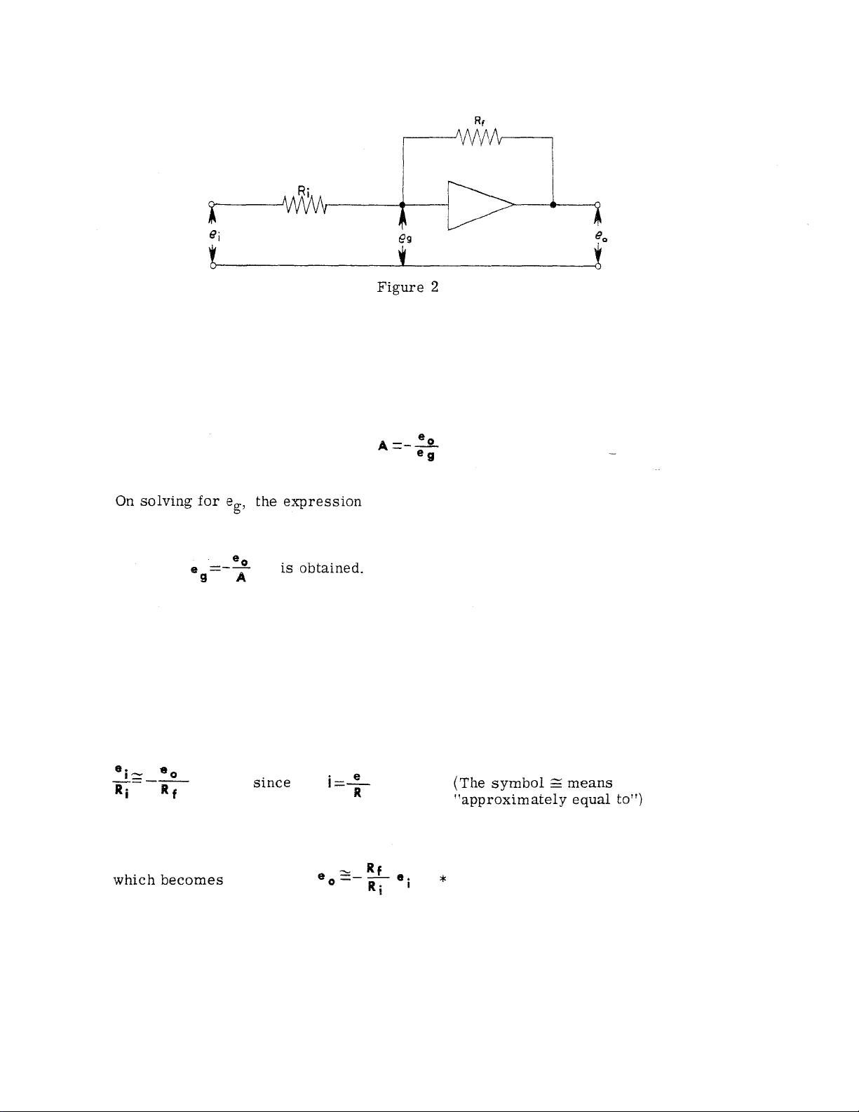
In use, resistors and capacitors are connected as input and feedback elements in such a way as to
perform various mathematical operations. For use as a multiplier, resistors are used as input
and feedback elements, as shown in Figure 2.
AMPLIFIER AS MULTIPLIER AND INVERTER
In this Figure, e
represents the input voltage, eg the grid voltage, eo the output voltage, Ri the
i
input resistor and Rf the feedback resistor.
The gain of an amplifier is given by
From this it can be seen that eg approaches zero as A approaches infinity. In practice, A is made
large with respect to e
by using high gain amplifiers so that eg becomes very small, and for
o
practical purposes eg can be considered to be at ground potential.
Since the input to the amplifier is the grid of a tube, the current through the amplifier from the
input can be considered to be zero, with the result that the current ii through the resistor Ri is, for
all practical purposes, equal to the current i
through the resistor Rf, with the result that
f
*For a more rigorous approach, see Korn and Korn, ELECTRONIC ANALOG COMPUTERS
(McGraw-Hill Book Company, Inc. , New York, 1956), Second Edition, Page 12.
Page 5
Page 6
The approximation which results from considering e = 0 will be used in the further discussion of
"
the DC amplifier but the "approximately equal to
considered to be equal to i
.
f
sign will not be used, that is, ii will be
In practice, the gain of DC computer amplifiers will vary from approximately 1000 for repetitive
computers to as high as 10 for a large commercial installation. Since the maximum output of an
amplifier is generally 100 volts, the value of eg will vary from about 0.1 volt to 1 micro-volt,
depending on the gain of the amplifier. Thus the amplifier gain is one factor in the accuracy of an
analog computer.
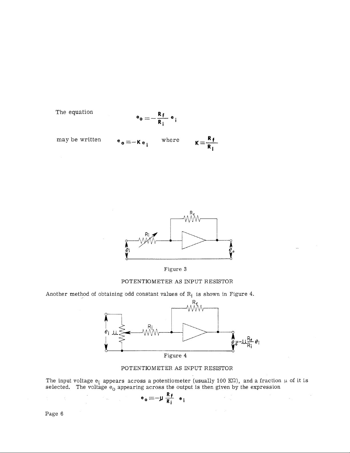
which is, in effect, multiplication by a constant. Since, in most cases, the output voltage is of the
opposite sign to the input voltage, the amplifier also acts as an inverter or sign changer.
To change the value of the constant K, it is necessary only to change R
at 1 megohm and R
is changed. This may be done by using a different value fixed resistor or by
i
using a potentiometer as shown in Figure 3.
or Rf. Generally, Rf is kept
i
Page 7
Suppose, for example, a ratio of 3.7 is desired. If is made equal to 0.37 and Rf/Ri = 10 (Rf = 1
megohm and R
= 100 K ohm), then eo = -3.7 ei. Generally this method is to be preferred over that
i
shown in Figure 3.
In actual practice, the ratio Rf/Ri is generally greater than unity, since the amplifiers tend to
become unstable for values less than unity. Also the ratio Rf/R
is 100 or less, as values greater
i
than 100 introduce inaccuracies in the solution of the problem.
If, instead of the one input resistor shown in Figure 2, two or more resistors are used as shown in
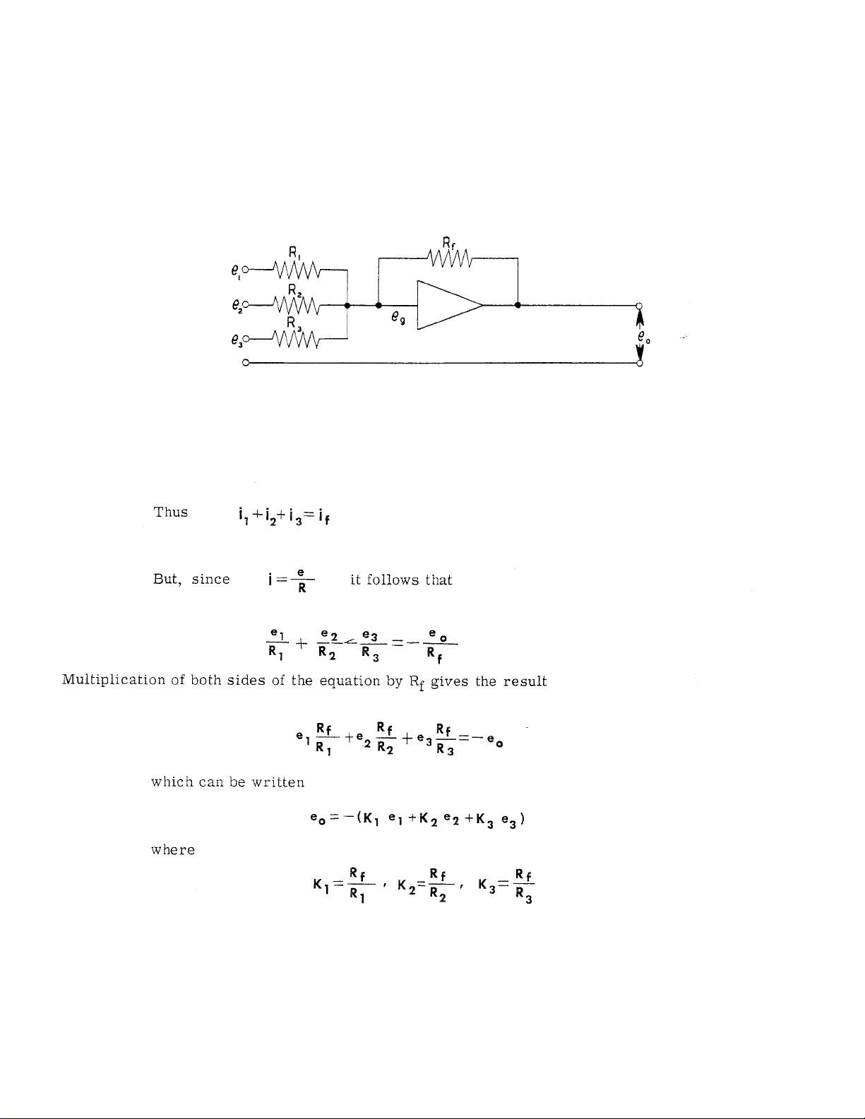
Figure 5, the operational amplifier becomes an adder.
Figure 5 AMPLIFIER AS ADDER
Again making use of eg 0, the sum of the currents in the input resistors equals the current
through the feedback resistor.
The operational amplifier can thus be used to add and at the same time multiply any of its in-puts
by constants. Any number of inputs can be used as long as the output voltage does not exceed the
nominal range of the amplifier.
Page 7
Page 8

Since subtraction can be considered to be the addition of negative numbers, subtraction can be
performed by using negative voltages for those quantities to be subtracted. The circuit shown in
g
Figure 6 would
ive the result
Figure 6
OPERATIONAL AMPLIFIER CIRCUIT USED FOR SUBTRACTION
Page 8
Page 9
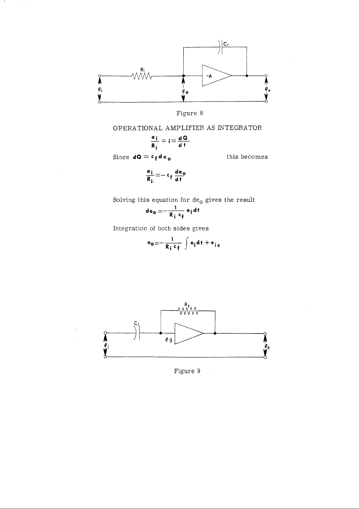
Where e
is the constant of integration
ic
(initial condition) and is the voltage
across the capacitor Cf at time t = o.
Thus the operational amplifier can integrate.
AMPLIFIER AS DIFFERENTIATOR
It is possible to show, by a similar analysis, that the operational amplifier can be used to
differentiate. The amplifier is used very seldom for this purpose, however, since noise in the input
tends to be magnified by differentiation, whereas it tends to cancel out in integration. Such
circuits also tend to be unstable.
In practice, the value of the feedback resistor Rf, when used, is generally 1 megohm and the value
of the feedback capacitor Cf, when used, is generally 1 microfarad. The value of the input resistor
usually varies from 0.1 megohm to 1.0 megohm, although in certain problems the values may be
different from these values.
g
e 10
Pa
Page 10

A combination of simple operations forms a complex operation. In general, an analog computer is
not used for addition alone or for multiplication by a constant as a single operation. These can be
better performed by other means. The value of the computer lies in its ability to combine these
simple operations into a complex operation.
An example of a complex operation is indicated by the circuit shown in Figure 10.
where eo (o) is the output voltage at time t = o (start of problem solution). Amplifier A is used for
sign inversion. It can be omitted if a minus result is acceptable.
Another example of a simple type of problem involving complex operation is that of an object
falling due to the force of gravity. The acceleration which the body experiences is constant near
the surface of the earth and due to the force exerted on the object by the gravitational field of the
earth. This may be written as an equation,
where y is the distance the object falls in time t, and g is the acceleration given the object by the
earth's gravitational field. By integrating twice, it is possible to obtain an expression for y in terms
of g and the time t during which the body has fallen. This can easily be set up on the computer,
using two amplifiers as shown in Figure 11.
Figure 11
AMPLIFIER CONNECTIONS FOR SOLVING "FALLING BODY PROBLEM"
The input voltage e
is supplied by a suitable power supply and the value of ei is chosen so that eo
i
does not exceed the output capacity of amplifier 2. Instructions for setting up this problem are
given on Page 21. It is suggested, however, that the actual setup and solution of the problem be
withheld until the CIRCUIT DESCRIPTION and OPERATION sections of this manual have been
thoroughly reviewed and are generally understood.
Page 11
Page 11

Other examples of the application of complex operation to the solution of problems are given in
the section on OPERATION.
SCALE FACTORS
In the operation of the analog computer two factors must be considered. The first of these is the
amplitude factor. In general, the output of each amplifier must be kept within the range ±100 volts,
the actual value depending on the amplifier used in the computer. In order to keep the output
within the specified limits, it is generally necessary to scale down the input voltages. It is not
always possible to determine before hand the range of the voltages, in which case a trial run can be
made and after the voltages are observed, the proper amplitude scale factors can be chosen.
Sometimes it is possible to estimate the range of voltages from the physics of the problem.
The other factor is time. If the product RiCf = 1 when Ri is measured in ohms and Cf is measured
in farads, the computation is said to be in real time. This is so, for example, when Ri = 1 megohm
6
and Cf = 1 µfd. (RiCf = 10
ohms x 10-6 farad = 1) If the computer is operated such that the
solution is obtained in less time than is required for the physical solution to occur, the operation is
said to be faster than real time. This is very useful if the physical occurrence which is being
simulated requires considerable time. Time is also saved, permitting the solution of more problems
in the same length of machine time.
Another advantage is that machine error is decreased, especially the error due to the leakage
resistance of the feedback capacitors. In general, the solution of a problem on the computer should
not require more than 1 to 5 minutes. Longer solution times require special precautions.*
REPETITIVE OPERATION
It is desirable, for many problems, to repeat the solution and observe the effect on the solution of
changing the various parameters of the problem. This is made possible by repetitive operation.
Some means is provided for automatically resetting the computer and re-running the problem. A
cathode ray oscilloscope is convenient for observing the solution in this case. Generally, one of the
computer amplifiers is used to provide the sweep for the oscilloscope . Details of operation will be
discussed in the section on OPERATION.
ACCURACY
As was shown previously, the higher the amplifier gain the less will be the error in each computing
operation. Thus the accuracy depends in part on the gain of the operational amplifier. Accuracy
also depends on the precision of the computing components, such as resistors and capacitors.
Time is also a factor in accuracy. In general, long runs introduce errors due to amplifier drift and
capacitor leakage.
* Goode and Machol, SYSTEM ENGINEERING (McGraw-Hill Book Company, Inc., New York, 1957),
Pages 278-283.
Clarence L. Johnson, ANALOG COMPUTER TECHNIQUES (McGraw-Hill Book Company, Inc. , New
York, 1956), Chapter 3, Pages 20-44.
Korn and Korn, ELECTRONIC ANALOG COMPUTERS (McGraw-Hill Book Company, Inc., New
York, 1956), Pages 30-35.
James B. Resnick, "Scale Factors for Analog Computers", Product Engineering, March, 1954.
Page 12
Page 12
Any variations in voltages in any part of the circuit of a direct-coupled amplifier cause variations
in the output voltage which in turn introduce errors in the solution. With constant input the
output will vary, resulting in "drift", which increases with amplifier gain. This introduces a
paradox since, as has been shown, error is reduced by increasing amplifier gain but this in turn
increases drift which increases errors. For this reason, very high gain amplifiers generally use
some means of stabilization in order to reduce drift. *
READ-OUT
For arithmetic problems in which a single numerical answer is obtained, the result can be read on
the meter. In problems having a continuous solution (changing with time) an oscilloscope is
desirable. It is possible in this case to watch the effect on the solution of varying the various
problem parameters. This is especially true when repetitive operation is used. In this case one of
the computer amplifiers is used to provide the sweep. The oscilloscope must be a DC scope.
If a permanent record of the solution is desired, a photograph of the oscilloscope trace may be
made or a recording galvanometer may be used. Examples of both methods are shown in the
illustrative problems.
NON-LINEAR OPERATION
A discussion of non-linear operation is beyond the scope of this manual. An excellent treatment of
non-linear operation can be found in ANALOG COMPUTER TECHNIQUES by Clarence L.
Johnson, Chapter 7, _Pages 107-127.
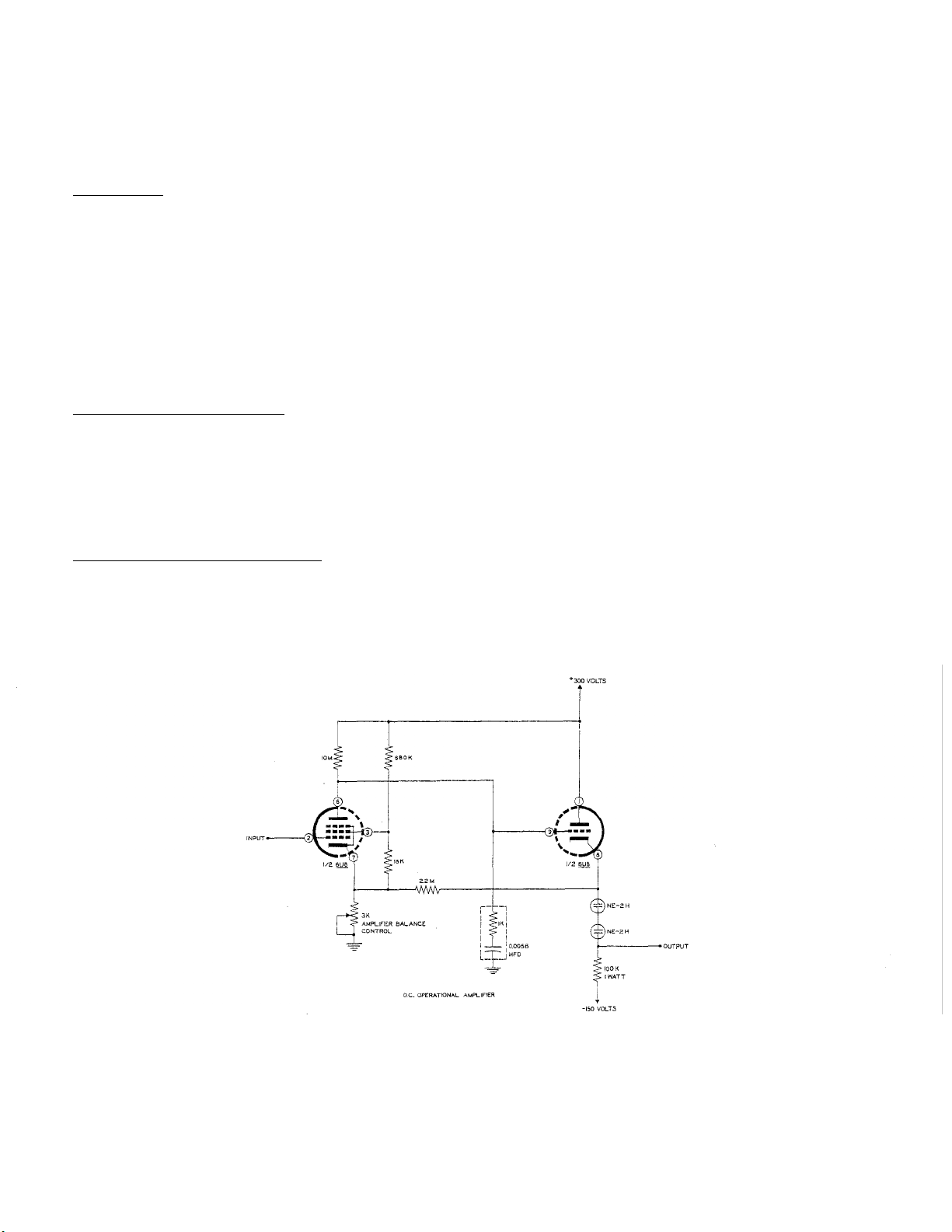
CIRCUIT DESCRIPTION
DC OPERATIONAL AMPLIFIER
The general requirements for a DC amplifier for computer use are high gain, high input impedance, low output impedance, good linearity and stability (low drift). The circuit of the amplifier
used in the Heath Analog Computer is shown in Figure
'
12.
Figure 12
DC OPERATIONAL AMPLIFIER FOR EC-1
* Korn and Korn, ELECTRONIC ANALOG COMPUTERS (McGraw-Hill Book Company, Inc., New
York, 1056) Second Edition, Pages 191-196 and 231-239.
Page 13
Page 13

The amplifier is designed around a 6U8 tube with which it is possible to achieve a gain of approximately 1000. This is adequate for the use for which this computer is designed. This high gain is
achieved by operating the pentode section of the 6U8 with a large plate load and with low volt-age
on the screen grid. * This gives a gain of approximately 700. The gain is increased to approximately 1000 by adding a small amount of positive feedback. The 2.2 megohm resistor provides this feedback. A high frequency filter consisting of a 1 K&2 resistor and a 5600 µµf capacitor
in series is used to prevent oscillation of the amplifier.
The 3 K2 control is used for adjusting the output of the amplifier to zero volts when there is no
input signal. One way of doing this (used in the EC-1) is to use a 1 megohm feedback resistor and
a 1 megohm resistor between input and ground, as shown in Figure 13.
AMPLIFIER BALANCE DIAGRAM
With the amplifier set up as in Figure 13, the 3 K2 zero adjust control is set for zero reading on
the meter. In the EC-1, this is accomplished by merely operating a switch to its BALANCE
position, which disconnects the amplifier from the problem board and connects the proper feedback and input resistors, thus simplifying the balancing operation.
The triode section of the 6U8 is connected as a cathode follower output stage. The two NE-2H
neon lamps are used as a reference voltage dropping element by which the output signal level can
be dropped from approximately 112 volts to zero volts without loss in gain, as would occur if a
purely resistive element were used.
The input and output terminals of the amplifier are on the panel or problem board with two of
each provided. These are so arranged that plug-in units may be easily and rapidly used to change
impedance values for various problems.
AMPLIFIER POWER SUPPLY
The +300 volt power supply is a conventional electronically regulated unit which provides the
+300 volts for operation of the amplifiers. The 250 K2 control adjusts the output voltage over a
range of approximately +250 to +350 volts. Provision is made for using the meter on the panel for
setting the voltage to +300 volts. The -150 volts DC required by the amplifier is supplied by a halfwave rectifier, the output of which is controlled by an OA2 regulator tube. The circuit is shown in
Figure 14.
* George E. Kaufer, "How to Design Starved Amplifiers", Tele-Tech and Electronic Industries, Vol.
14, No. 1, January 1955, Page 68.
Walter K. Volkers, "Ultra-High-Gain Direct-Coupled Amplifier Circuits", - paper read before 1950
IRE National Convention in New York.
Page 14
Page 14

+300 VOLT D.C. POWER SUPPLY
Figure 14
+300 VOLT DC POWER SUPPLY FOR EC-1
INITIAL CONDITION POWER SUPPLIES
The voltages for the initial conditions or the "given" quantities of the problem are supplied by
three initial condition power supplies. These use conventional half-wave rectifiers with OB2
regulator tubes and potentiometers so that any voltage from 0-100 may be obtained. The supplies are ungrounded, making them usable for either plus or minus voltages with respect to
amplifier ground.
CONTROL CIRCUIT
While the amplifiers perform the actual mathematical operations, it is necessary to provide
certain control functions. Before solution of the problem can commence, the voltage of the
amplifier must be set to the proper value and the amplifiers must be balanced. Provision is made
for this by means of a meter and a FUNCTION switch on the panel. By use of the FUNCTION
switch and meter, the output of any of the operational amplifiers may also be measured . An
OPERATION switch turns the computer on, starting solution of the problem. After the problem is
solved, it is necessary to reset the computer to the starting conditions,. This is accomplished by
setting the OPERATION switch to the RESET position, which operates a relay which in turn
removes residual voltages from the amplifiers and resets initial condition voltages so that the
computer is ready to again solve the problem.
REPETITIVE OSCILLATOR
Sometimes it is desirable to automatically repeat the solution a number of times. This is
accomplished in the EC-1 by means of a multivibrator which cycles the relay at an adjustable
rate of from approximately 0.1 to 15 times per second. In this way the effect on the solution of
changing any of the problem parameters may be observed. The rate of repetition is changed by a
control on the panel.
Page 15
Page 15

GENERAL OPERATING INSTRUCTIONS
Electrical power for the computer is controlled by two toggle switches marked FILAMENT and
HIGH VOLTAGE, with green and clear pilot lamps, respectively. These switches are wired so that
the filaments may be on with the high voltage off, but the high voltage will not be on unless the
filament switch is in the ON position. Thus the filaments may be left on when the computer is not
in actual use, doing away with the warming-up time otherwise necessary. The filaments should
be turned on several minutes (preferably at least one-half hour) before use and should then be
left on unless the computer is to be idle for a period of several hours or longer.
To adjust the amplifier power supply output, the METER FUNCTION switch is set to SET B+.
The OPERATION switch should be in the RESET position. With the HIGH VOLTAGE switch ON,
turn the control VC on the chassis (near the rear) until the meter pointer rests at the red mark
labeled SET B+. This sets the output of the amplifier power supply to +300 volts.
Leaving the OPERATION switch in the RESET position, set the METER RANGE switch to 100 V
and the METER FUNCTION switch to AMPLIFIER BALANCE. Starting with amplifier 1, press
downward the slide switch immediately below the amplifier terminals on the panel and, using a
screwdriver, turn the AMPLIFIER BALANCE CONTROL until the meter pointer reads zero. Repeat
this operation for each of the other eight amplifiers. With the METER RANGE switch set at 10 V,
repeat the above operation for each amplifier. Once again, repeat the above operation for each
amplifier with the METER RANGE switch set at 1 V. The amplifiers should be checked for
balance before each problem run. It is not necessary to remove computing components from the
problem board when balancing amplifiers as the slide switch on the panel disconnects the
amplifier from the problem board, as shown in Figure 15.
Figure 15 AMPLIFIER BALANCE CIRCUIT
Two binding posts above and to the right of the meter provide for external use of the meter. With
the METER FUNCTION switch in INPUT position, the meter is disconnected from the computer
and connected to the two binding posts labeled METER INPUT. The meter may then be used to
measure voltages of 100 or less applied to the METER INPUT binding posts. The METER RANGE
switch is used to select the proper range. The meter has a sensitivity of 10,000 ohms per volt.
The AMPLIFIER OUTPUT binding posts above and to the left of the meter provide for external
read-out, such as with an oscilloscope or pen recorder. By turning the METER FUNCTION switch
to any of the positions 1 through 9, the output of the corresponding amplifier may be read on the
meter or taken off at the terminals marked AMPLIFIER OUTPUT. If desired, the METER RANGE
switch may be set to OFF, thus disconnecting the meter from the output circuit and using only
the binding posts. The AMPLIFIER OUTPUT terminals are automatically disconnected
Page 16
Page 16

from the meter when the METER FUNCTION switch is at SET B+ or INPUT, making it unnecessary
to disconnect the external read-out unit when checking the power supply voltage. Likewise, the
METER INPUT terminals are disconnected at all positions of the METER FUNCTION switch except
INPUT.
The outputs of the three initial condition power supplies are connected to binding posts on the
panel immediately under the controls for the supplies. The outputs are not grounded, making it
possible to use either the plus (red) or minus (black) terminal for the "hot" terminal. Since the
supplies are not grounded, it is necessary to ground one of the terminals of each supply in use.
The output is zero when the control is full counterclockwise; turning the control clockwise
increases the output up to 105 volts, with a maximum current of 5 ma.
Five coefficient potentiometers are provided on the panel. One end terminal is grounded, with the
other end terminal and the center terminal connected to binding posts on the panel. The center
terminal of the control (black binding post) is grounded when the control is in full counter-clockwise
position. The ungrounded end terminal (red binding post) will be connected to the IC supply
voltage of the required potential.
A 4PST relay is used for inserting initial conditions and for removing residual voltages from the
amplifiers. For convenience, the connections to the relay contacts are brought to binding posts on
the panel where they may be connected across problem components as required. The relay
contacts are normally closed. Turning the OPERATION switch to MANUAL will start solution of a
problem by opening the relay contacts, which will remain open until the switch is returned to
RESET. Setting the OPERATION switch to REPETITIVE will connect the relay to the repetitive
oscillator, opening and closing the contacts at a rate determined by the REPETITION RATE control
on the panel. Turning the control clockwise increases the rate of operation from the minimum of
approximately 0.1 cps to the maximum of approximately 15 cps.
Computing components are connected to the amplifiers by means of 2-prong plugs inserted into
sockets on the panel. Suggested methods of mounting components on the plugs are shown in
Figure 25 in the Construction Manual.
BASIC MATHEMATICAL OPERATIONS
ADDITION
Two quantities can be added by feeding two voltages, proportional to the quantities, into an
amplifier, as shown in Figure 16.
Figure 16
AMPLIFIER USED FOR ADDITION
Page 17
Page 17

As an example, consider .the simple problem of finding the sum of 36 + 58. Since the sum of these
numbers is greater than 60, the voltages used cannot be equal to the numbers but must be scaled
down. In this case, voltages equal to 1/10 of the numbers will be suitable. The problem setup now
looks like Figure 17.
Figure 17
AMPLIFIER USED FOR ADDITION
Since the input voltages are equal to 1/-10 of the quantities being added, the output voltage will be
1/10 of the sum and so must be multiplied by 10 to obtain the answer. Notice that the answer is
negative with respect to the inputs. If this is undesirable, a second amplifier may be used for sign
inversion. See Figure 18.
The voltages are obtained from the initial condition power supplies and the answer is read on the
meter. Turn on the FILAMENT switch, after having plugged 1 megohm 1% precision resistors,
previously mounted on 2-prong plugs, into the two input sockets and the feedback socket of
amplifier 1. Plug in a patch cord between the black binding post of initial condition power supply 1
and the black binding post marked METER INPUT which is above the meter. Connect another patch
cord from the red binding post of IC-1 (initial condition power supplies will hereafter be called IC)
and the red binding post marked METER INPUT. Set the METER FUNCTION switch at 10 V and
the number 1 INITIAL CONDITION control to extreme counterclockwise position. Turn on the
HIGH VOLTAGE switch and turn the IC-1 control clockwise until the meter reads 3.6 volts. Now
unplug the end of the patch cord at the red METER INPUT binding post and plug it into either of the
INPUT binding posts of amplifier 1. In the same manner, connect IC-2 to the meter (connect the
black binding post of IC-2 to the black binding post marked ME TER INPUT) and set the control IC-2
so the meter reads 5.8 volts. Unplug the end of the patch cord at the red METER INPUT binding
post and plug it into the other INPUT binding post of amplifier 1. Set the METER FUNCTION
switch to AMPLIFIER OUTPUT 1 and read the voltage on the meter. Multiply this reading by 10 to
obtain the answer. CAUTION: In general, before using the meter for reading an answer, the METER
RANGE switch should be on the 100 V range so as not to damage the meter if the result exceeds 10
V. In this case, we knew the answer would be less than 10 V. Also remember that the output of any
amplifier should not exceed ±60 volts.
Since the red binding posts of the IC power supplies are connected to the amplifier inputs, the input
voltages are positive
The output read on the meter is negative (-) however, due to the action of the amplifier as an inverter
or sign changer. A plus answer can be obtained by use of a second amplifier with unity gain (Ri =
Rf, generally 1 megohm in each case). This is shown in Figure 18.
H.
Page 18
Page 18

MULTIPLICATION
Multiplication by a constant is performed by using different values of input resistor and feed-back
resistor. As an example, find the product of 10 x 37. See Figure 19. Plug a 100 K, 1% precision
resistor into either input socket and a 1 megohm resistor into the feedback socket of amplifier 1.
Set IC-1 to 3.7 volts and then connect this voltage to that input of amplifier 1 to which the 100 K
ohm resistor was connected. Read the output on the meter and multiply this reading by 10 to
obtain the answer. (The 37 was divided by 10 in order to keep the result under 60 volts.) Again
notice the result is negative with respect to the input, due to the 180 phase shift in the am
p
lifier.
INTERGRATION
It was shown on Page 10 that by replacing the feedback resistor of an amplifier with a capacitor,
the output of the amplifier is proportional to the integral of the input voltage, or more specific-ally,
Plug a 1 megohm precision resistor into either of the input sockets and a 1 µfd mylar capacitor
into the feedback socket of amplifier 1. When using an amplifier as an integrator, it is necessary to
remove the charge on the capacitor before using the amplifier again. If this is not done, an error
will be introduced in the next solution due to this residual change. In the EC-1, this is
accomplished by connecting a pair of the relay contacts across the feedback capacitor; the contacts are closed when the amplifier is not integrating and open when the computer is operating, as
shown in Figure 20 on Page 20.
Page 19
Page 19

When the OPERATION switch is in the RESET position, the relay contacts are all closed.
Connect the two binding posts on either end of the feedback socket to the two relay contacts 1, as
shown in Figure 21. Set IC-1 to 5 volts and connect to the input of amplifier 1, to which the 1
megohm resistor was connected. Turn the OPERATION switch to MANUAL. The meter reading
should increase rather uniformly from zero to approximately 100 V, but should be stopped at 60
volts by turning the OPERATION switch to RESET. This will stop integration and remove the
charge from the capacitor, leaving it ready for operation again. Turning the OPERATION switch to
REPETITIVE will start the computer operating, but now the oscillator will automatically reset the
initial conditions and start solution again at a rate control by the REPETITION RATE control. This
operation will continue until the OPERATE switch is returned to RESET.
. Page 20
Page 20

The operations just carried out illustrate the basic operations performed by the computer, but the
real value of the computer lies in combining these elementary operations in such a way as to solve
problems.
ILLUSTRATIVE PROBLEMS
The operations just described are the basic operations which can be performed by the computer.
They are given to illustrate the method of setup and operation rather than because they are useful
in themselves. Only when the basic operations are combined for the solutions of complex
problems does the computer become a valuable tool for problem solving.
The following problems will illustrate some of the types of problems, the solution of which can
readily be obtained on the computer.
Components are furnished for use in solving some of these problems. For other problems,
additional components are required. These may be standard radio components. Ordinary 5% or
10% resistors may be used where accuracy of results is not important, such as when only the
general nature of the problem solution is needed.
Additional problems will be found in the references at the back of the manual.
FALLING BODY PROBLEM: One of the simplest problems encountered in elementary physics is
that of a body moving under the influence of a constant force, such as the earth's gravitational
field near the surface of the earth. The equation for the motion of a body in such a field is
where g is the acceleration which a body experiences when in the earth's gravitational field and y
is the distance the body falls in time t. To find the value of y, it is necessary to integrate twice.
Page 21
Page 21

The value of g is supplied by one of the IC power supplies. Some way must be provided for discharging the capacitors at the end of the solution of the problem. This can be accomplished by
connecting the capacitor to the relay contacts which are open during solution of the problem and
closed during the "reset" time.
The 100 K potentiometer is the IC potentiometer. Connect a patch cord from the red binding post
of IC-1 to the INPUT binding post of amplifier 1, and another patch cord from the black binding
post of IC-1 to the black METER INPUT binding post above the meter. Plug a 1 megohm mounted
resistor into the input socket of amplifier 1 (the one to which the patch cord is connected) and a 1
megohm resistor into either input socket of amplifier 2. Plug mounted 1 µfd capacitors into the
feedback sockets of amplifiers 1 and 2. Connect a patch cord (short) from the output of amplifier 1
to the input of amplifier 2 (the one with the 1 megohm resistor). Connect patch cords from the
AMPLIFIER INPUT binding post and AMPLIFIER OUTPUT binding posts to relay contacts 1 for
amplifier 1 and relay contacts 2 for amplifier 2. Set IC-1 control to the first or second dot from the
extreme counterclockwise direction. Set the METER RANGE switch to 100 V and the METER
FUNCTION switch to AMPLIFIER OUTPUT 2. Turn the HIGH VOLT-AGE switch to ON (the filament
switch should previously have been turned to ON). Turn the OPERATION switch to MANUAL. The
meter needle should move to the right, slowly at first, gaining speed as it moves. When the needle
.
reaches 60-65 volts, turn the OPERATION switch to RESET which will discharge the capacitors,
making the computer ready to again solve the problem. If the meter needle moves too slowly, turn
the IC control clockwise; if the needle
Page 22
Page 22

moves too rapidly, turn the control counterclockwise. Turn the OPERATION switch to REPETITIVE.
The computer will now reset itself and repeat the solution at a rate controlled by the REPETITION
RATE control knob. This will continue until the OPERATION switch is returned to the RESET
position. If a permanent record of the solution is desired, a pen recorder may be connected to the
AMPLIFIER OUTPUT binding posts above the meter.
The solution may be viewed on a DC oscilloscope, such as the Heath DC Oscilloscope, by connecting the vertical input of the oscilloscope to the red AMPLIFIER OUTPUT binding post and the
ground to the black AMPLIFIER OUTPUT binding post. No sweep is needed to show the falling body,
but if one wants to show the path when an initial horizontal velocity is given the body, a sweep
voltage is necessary. To insure synchronization, one of the computer amplifiers should be used as
the sweep generator for the oscilloscope, as shown in Figure 26.
The ±100 volts is obtained from one of the IC power supplies, using + or -, depending on the
direction of sweep desired. Set the IC control until the desired rate of sweep is obtained. The
values of R
If a faster rate of solution is desired, the 1 megohm resistors should be replaced by 0.1 megohm
resistors and the 1 microfarad capacitors by 0.1 microfarad capacitors, adjusting the REPETITION
RATE control accordingly.
and of Cf should be the same as those used in the problem.
i
Page 23
Page 23

This circuit is setup on the computer as before, with the addition of a feedback resistor across the
first amplifier. For simplicity, the relay and ground connections are omitted as well as the initial
condition power supply connections. These are the same as in the previous problem.
The solution is shown in Figure 28.
Page 24
Page 24

The differential equation of the spring-mass system shown in Figure 29 is
g
The differential equation may be written
The simplified computer diagram is shown in Figure 30.
In this diagram all resistor values are megohms and all capacitor values are microfarads. Ground
connections are omitted for purpose of simplicity. F (t) is supplied by one of the initial condition
power supplies.
Various solutions are shown in Fi
ure 31.
Page 25
Page 25

SIMULTANEOUS ALGEBRAIC EQUATIONS
A different type of problem is one involving simultaneous algebraic equations. A system of two
equations in two unknowns may be represented by the equations
These equations may be rewritten in the form
The computer circuit for these equations is shown in Figure 32.
As an example, consider the equations
5X + 3 Y = 210
2 x + 5 Y = 160
These equations become
X/3 + Y / 5 = 14
X/5 + Y / 2 = 16
Page 26
Page 26

The computer circuit for these equations is shown in Figure 33.
The values of x and y are read on the meter.
Control A is set so that the voltage drop between the center lugs and ground is 1/3 the voltage
drop across the control. Control B is set so that the voltage drop between the center lug and
ground is 1/5 the voltage drop across the control. Controls C and D are likewise set for 1/2 and
1/5 the total voltage respectively.
PROJECTILE PROBLEM
A variation of the falling body problem is to fire a projectile upward at an angle from the horizontal
and see the path on the oscilloscope. * Air resistance may be introduced also. Thus the effects of
the initial velocity, gravity and air resistance may be observed.
In the X direction, the equation of motion is
and the equation in the Y direction is
*The setup of this problem is presented here through the courtesy of Prof. Harry F. Meiners of the
Department of Physics, Rensselaer Polytechnical Institute, Troy, New York.
Page 27
Page 27

The basic computer setup is shown in Figure 34.
The components of the initial velocity are controlled by IC-1 and IC-2, while the acceleration due
to gravity, g, is controlled by IC-3. Air resistance is controlled by the controls m/c. The solution is
shown in Figure 35.
BOUNCING BALL
A problem which is interesting to watch, as well as one which illustrates the more complex type of
problem that the computer is capable of handling, is the "Bouncing Ball" problem. For solving this
problem, a few additional components are required which are readily obtained from most any
dealer in radio supplies. The following additional components are needed:
Page 28
Page 28

1 20 K ohm (0.02 megohm) resistor
1 200 K ohm (0.2 megohm) resistor
1 500 K ohm (0.5 megohm) resistor
1 2 megohm resistor
1 5 megohm resistor
4 10 megohm resistors
The resistors should preferably be 1% tolerance, but 5% or even 10% resistors will be satisfactory
for demonstration purposes. The potentiometers can be of the ordinary radio type. Silicon diodes
are furnished with the computer. In addition to the above components, it is necessary to set up a
phase shifter to produce the Lissajous pattern which simulates the ball. The parts required for the
unit are:
1 6.3 V filament transformer (current rating not
important but must have center tap)
10 KO, 1/2 watt resistors
25 K ohm controls
0.1 µfd, 150 volt capacitor
1.0 µfd, 150 volt capacitor
100 KO controls
These components are standard radio components. The capacitors may be paper or plastic
tubular. The complete diagram for the problem, including the phase shifter, is shown in Figure 38.
Any good DC oscilloscope may be used for observing the motion of the ball. The Heath DC
Oscilloscope is especially suitable for use with the EC-1. The sweep circuit in the oscilloscope is
not used, as the sweep voltage is provided by the computer. Solution is shown in Figure 37.
Page 29
Page 29

Page 30

REFERENCE BOOKS
ANALOG COMPUTERS
Goode, Harry H. and Machol, Robert E., SYSTEM ENGINEERING, McGraw-Hill, 1957.
Johnson, Clarence L. , ANALOG COMPUTER TECHNIQUES, McGraw-Hill, 1956.
Karplus, Walter J., ANALOG SIMULATION, McGraw-Hill, New York, 1958. (Chapter 9).
Korn, Granino A. and Korn, Theresa M., ELECTRONIC ANALOG COMPUTERS, Second Edition,
McGraw-Hill, 1956.
Paynter, H. M. , A PALIMPSEST ON THE ELECTRONIC ANALOG ART, Geo. A. Philbrick Re-
searches, Inc., 230 Congress Street, Boston, Massachusetts, 1955.
Smith, George W. and Wood, Roger C., PRINCIPLES OF ANALOG COMPUTATION, McGraw-Hill,
1959.
Soroka, Walter W. , ANALOG METHODS IN COMPUTATION AND SIMULATION, McGraw- Hill,
1954.
Wass, C. A. A., INTRODUCTION TO ELECTRONIC ANALOGUE COMPUTERS, McGraw-Hill,
1955.
ANALOG AND DIGITAL COMPUTERS _
Berkeley, Edmund C. and Wainwright, Lawrence, COMPUTERS - THEIR OPERATION AND
APPLICATIONS, Reinhold, New York, 1956.
Engineering Research Associates Staff, HIGH-SPEED COMPUTING DEVICES, McGraw-Hill,
1950.
Ivall, T. E. , ELECTRONIC COMPUTERS - PRINCIPLES AND APPLICATIONS, Philosophical
Library, New York, 1956.
Proceedings of the NATIONAL ELECTRONICS CONFERENCE, Volume V, 1949, Chicago, 1950.
PAMPHLETS
Howe, C. E. and Howe, R. M. , A TABLETOP ELECTRONIC DIFFERENTIAL ANALYZER,
University of Michigan, Department of Aeronautical Engineering, Publication AIR-6, 1953.
Martinez, Hugo, AN INTRODUCTION TO THE APPLICATION OF ELECTRONIC ANALOG
COMPUTERS, Berkeley Division of Beckman Instruments Inc. , 2200 Wright Avenue, Richmond 3, California.
Nichols, M. H. and Hagelbarger, D. W. , A SIMPLE ELECTRONIC DIFFERENTIAL ANALYZER AS
A DEMONSTRATION AND LABORATORY AID TO INSTRUCTION ON ENGINEERING,
University of Michigan, Department of Aeronautical Engineering, 1951.
Haneman, V. S. Jr. and Howe, R. M. , SOLUTION OF PARTIAL DIFFERENTIAL EQUATIONS BY
DIFFERENCE METHODS USING THE ELECTRONIC DIFFERENTIAL ANALYZER, University
of Michigan, Department of Aeronautical Engineering, Engineering Research Institute,
Publication AIR-1, 1951.
ARTICLES
Page 31

Resnick, James B. , "Scale Factors For Analog Computers", Product Engineering, March, 1954.
Page 31
Page 32

Reque, S. G. , "Simulate the System With an Analog Computer", Control Engineering, September,
1956, Pages 138-144.
Heald, Carl, "Putting the Analog Computer to Work", ISA Journal, Vol. 3, No. 8, August 1956,
Page 270.
Howe, R. M. , and Haneman, V. S. , "Solution of Partial Differential Equations by Difference
Methods Using the Electronic Differential Analyzer", Proceedings IRE, Vol. 41, No. 10,
October, 1953.
Strong, John D., "A Practical Approach to Analog Computers", Instruments and Automation, Vol.
28, No. 4, April, 1955.
Symon, Keith R. and Poplawsky, "An Electronic Differential Analyzer", American Journal of
Physics, Vol. 21, No. 1, January 1953, Page 53.
Martinez, Hugo M., "Operational Electronic Analog Computers", ISA Journal, March and April
1957.
JOURNAL
IRE TRANSACTIONS ON ELECTRONIC COMPUTERS, Published quarterly by The Institute of
Radio Engineers, 1 East 79th Street, New York 21, New York.
SPECIFICATIONS
AMPLIFIERS:
Nine DC Operational Amplifiers using one 6U8 per amplifier.
Open loop gain approximately 1000.
Output -60 to +60 volts at 3 ma.
Two inputs and two outputs per amplifier.
Provision on panel for balancing amplifiers without removing problem setup.
Computing components mount on 2-prong plugs which fit into sockets on panel.
Power requirements - nine amplifiers. +300 volts at 25 ma. -150 volts at 40 ma.
POWER SUPPLIES:
+300 volts at 25 ma electronically regulated. Variable from +250 to +350 volts with provision for setting to +300 volts using meter on panel.
-150 volts at 40 ma regulated by VR tube.
Three initial condition power supplies providing 0 to 100 volts at 5 ma regulated by VR tube.
COEFFICIENT POTENTIOMETERS:
Five 100 K ohm potentiometers with terminals on panel.
REPETITIVE OPERATION:
A multivibrator provides for:
Repetitive operation at from approximately 0.1 to 15 cps.
Multivibrator operates relay with four sets of contacts.
Page 32
Page 33

METER:
50-0-50 microampere movement.
Reads 1-0-1, 10-0-10, 100-0-100 volts DC.
Panel switch selects output of any amplifier.
Provision for setting B+ power supply voltage.
Reads output of amplifiers for balancing amplifiers.
Terminals provided for external read-out such as CRO, recording galvanometer, etc.
COMPUTING COMPONENTS:
Precision resistors, Mylar capacitors, diodes and patch cords are provided for setting up
illustrative problems given in the instruction manual.
POWER REQUIREMENTS:
105-125 volts 50-60 cycles 100 watts
DIMENSIONS:
19 5 /8" wide, 11 1/2" high, 15" deep.
APPLICATIONS:
Teaching and demonstration in Engineering, Physics and Mathematics classes.
Laboratory use, especially in classes in analog computer design and use.
Industrial laboratories for preliminary runs of problems.
Page 33
Page 34

Page 35

Page 34
Page 36

Page 35
Page 37

Page 36
Page 38

Page 37
Page 39

Page 38
Page 40

 Loading...