HAMEG HZ530 User Manual

Download

Near Field Probes

HZ530

Handbuch / Manual / Manual

Deutsch / English / Español

CE Konformität CE marking

Conformidad CE .................................. 3

Deutsch ................................................ 4

English................................................ 23

Español............................................... 47

290601-zim/tke

Printed in Germany

Allgemeine Hinweise zur CE-Kennzeichnung

HAMEG Meßgeräte erfüllen die Bestimmungen der EMV Richtlinie. Bei der Konformitätsprüfung werden von HAMEG die gültigen Fachgrund- bzw. Produktnormen zu Grunde gelegt. In Fällen wo unterschiedliche Grenzwerte möglich sind, werden von HAMEG die härteren Prüfbedingungen angewendet. Für die Störaussendung werden die Grenzwerte für den Geschäfts- und Gewerbebereich sowie für Kleinbetriebe angewandt (Klasse 1B). Bezüglich der Störfestigkeit finden die für den Industriebereich geltenden Grenzwerte Anwendung. Die am Meßgerät notwendigerweise angeschlossenen Meß- und Datenleitungen beeinflussen die Einhaltung der vorgegebenen Grenzwerte in erheblicher Weise. Die verwendeten Leitungen sind jedoch je nach Anwendungsbereich unterschiedlich. Im praktischen Meßbetrieb sind daher in Bezug auf Störaussendung bzw. Störfestigkeit folgende Hinweise und Randbedingungen unbedingt zu beachten:

1. Datenleitungen

Die Verbindung von Meßgeräten bzw. ihren Schnittstellen mit externen Geräten (Drukkern, Rechnern, etc.) darf nur mit ausreichend abgeschirmten Leitungen erfolgen. Sofern die Bedienungsanleitung nicht eine geringere maximale Leitungslänge vorschreibt, dürfen Datenleitungen (Eingang/Ausgang, Signal/Steuerung) eine Länge von 3 Metern nicht erreichen und sich nicht außerhalb von Gebäuden befinden. Ist an einem Geräteinterface der Anschluß mehrerer Schnittstellenkabel möglich, so darf jeweils nur eines angeschlossen sein. Bei Datenleitungen ist generell auf doppelt abgeschirmtes Verbindungskabel zu achten. Als IEEE-Bus Kabel sind die von HAMEG beziehbaren doppelt geschirmten Kabel HZ72S bzw. HZ72L geeignet.

2. Signalleitungen

Meßleitungen zur Signalübertragung zwischen Meßstelle und Meßgerät sollten generell so kurz wie möglich gehalten werden. Falls keine geringere Länge vorgeschrieben ist, dürfen Signalleitungen (Eingang/Ausgang, Signal/Steuerung) eine Länge von 3 Metern nicht erreichen und sich nicht außerhalb von Gebäuden befinden. Alle Signalleitungen sind grundsätzlich als abgeschirmte Leitungen (Koaxialkabel - RG58/ U) zu verwenden. Für eine korrekte Masseverbindung muß Sorge getragen werden. Bei Signalgeneratoren müssen doppelt abgeschirmte Koaxialkabel (RG223/U, RG214/U) ver-

wendet werden.

3. Auswirkungen auf die Meßgeräte

Beim Vorliegen starker hochfrequenter elektrischer oder magnetischer Felder kann es trotz sorgfältigen Meßaufbaues über die angeschlossenen Meßkabel zu Einspeisung unerwünschter Signalteile in das Meßgerät kommen. Dies führt bei HAMEG Meßgeräten nicht zu einer Zerstörung oder Außerbetriebsetzung des Meßgerätes. Geringfügige Abweichungen des Meßwertes über die vorgegebenen Spezifikationen hinaus können durch die äußeren Umstände in Einzelfällen jedoch auftreten

Dezember 1995

HAMEG GmbH

Änderungen vorbehalten / Subject to change without notice

KONFORMITÄTSERKLÄRUNG DECLARATION OF CONFORMITY DECLARATION DE CONFORMITE

Name und Adresse des Herstellers HAMEG Instruments GmbH Manufacturer´s name and address Industriestraße 6 Nom et adresse du fabricant D - 63533 Mainhausen

Die HAMEG Instruments GmbH bescheinigt die Konformität für das Produkt The HAMEG Instruments GmbH herewith declares conformity of the product HAMEG Instruments GmbH déclare la conformite du produit

Bezeichnung / Product name / Designation:

Typ / Ty pe / Typ e:

mit / with / avec:

Optionen / Options / Options:

mit den folgenden Bestimmungen / with applicable regulations / avec les directives suivantes

EMV Richtlinie 89/336/EWG ergänzt durch 91/263/EWG, 92/31/EWG EMC Directive 89/336/EEC amended by 91/263/EWG, 92/31/EEC Directive EMC 89/336/CEE amendée par 91/263/EWG, 92/31/CEE

Niederspannungsrichtlinie 73/23/EWG ergänzt durch 93/68/EWG Low-Voltage Equipment Directive 73/23/EEC amended by 93/68/EEC Directive des equipements basse tension 73/23/CEE amendée par 93/68/CEE

Angewendete harmonisierte Normen / Harmonized standards applied / Normes harmonisées utilisées

Sicherheit / Safety / Sécurité

EN 61010-1: 1993 / IEC (CEI) 1010-1: 1990 A 1: 1992 / VDE 0411: 1994 Überspannungskategorie / Overvoltage category / Catégorie de surtension: II Verschmutzungsgrad / Degree of pollution / Degré de pollution: 2

Elektromagnetische Verträglichkeit / Electromagnetic compatibility / Compatibilité électromagnétique

EN 50082-2: 1995 / VDE 0839 T82-2 ENV 50140: 1993 / IEC (CEI) 1004-4-3: 1995 / VDE 0847 T3 ENV 50141: 1993 / IEC (CEI) 1000-4-6 / VDE 0843 / 6 EN 61000-4-2: 1995 / IEC (CEI) 1000-4-2: 1995 / VDE 0847 T4-2: Prüfschärfe / Level / Niveau = 2

EN 61000-4-4: 1995 / IEC (CEI) 1000-4-4: 1995 / VDE 0847 T4-4: Prüfschärfe / Level / Niveau = 3

EN 50081-1: 1992 / EN 55011: 1991 / CISPR11: 1991 / VDE0875 T11: 1992

Gruppe / group / groupe = 1, Klasse / Class / Classe = B

Near Field Sniffer Probes

HZ530

Datum /Date /Date Unterschrift / Signature /Signatur

23.01.1996

Dr. J. Herzog Technical Manager Directeur Technique

Änderungen vorbehalten / Reservado el derecho de modiﬁ cación

Inhaltsverzeichnis

Bedienungsanleitung

HZ530-Sondensatz für EMV-Diagnose ................................... 5

Bedienungsanleitung .............................................................. 7

Allgemeines ............................................................................. 7

Symbole ................................................................................... 7

Sicherheit.................................................................................. 7

Betriebsbedingungen ............................................................. 8

Gewährleistung ........................................................................ 8

Grundlagen der Meßtechnik mit Nahfeldmeßsonden .......... 9

Die H-Feld-Sonde ..................................................................... 9

Die Hochimpedanzsonde ........................................................ 9

Der E-Feld-Monopol ...............................................................10

Inbetriebnahme .......................................................................10

Sicherheitshinweis! ................................................................12

Applikationen für die Nahfeldsonden HZ 530 ......................13

Messung der Schirmdämpfung von Abschirmgehäusen ... 20

mit der E-Feld-Sonde ............................................................. 20

Operating instruction .......................................................... 23

Änderungen vorbehalten / Subject to change without notice

HZ530-Sondensatz für EMV-Diagnose

Technische Daten

Frequenzbereich:

100 kHz – ≥ 1000 MHz

(untere Grenzfreq. abhängig von Sondentyp)

Ausgangsimpedanz: 50Ω Anschluß: BNC-Buchse Eingangskapazität: ca. 2pF (Hoch-

impedanzsonde)

Max. Eingangspegel: +10dBm

(Zerstörungsfrei)

1dB-Kompressionspunkt: -2dBm

(frequenzabhängig)

Max. DC-Eingangsspg.: 20V Versorgungsspannung: 6V DC

Versorgungsspanung aus 5010/5011 oder 4 X 1.5 V Mignon Zelle

Stromaufnahme:

ca. 8mA; H-Feld Sonde ca. 15mA; E-Feld Sonde ca. 24mA; Hochimpedanzsonde

Sondenmaße: 40x19x195 mm (BxHxL) Gehäuse: Kunststoff

innen elektrisch geschirmt.

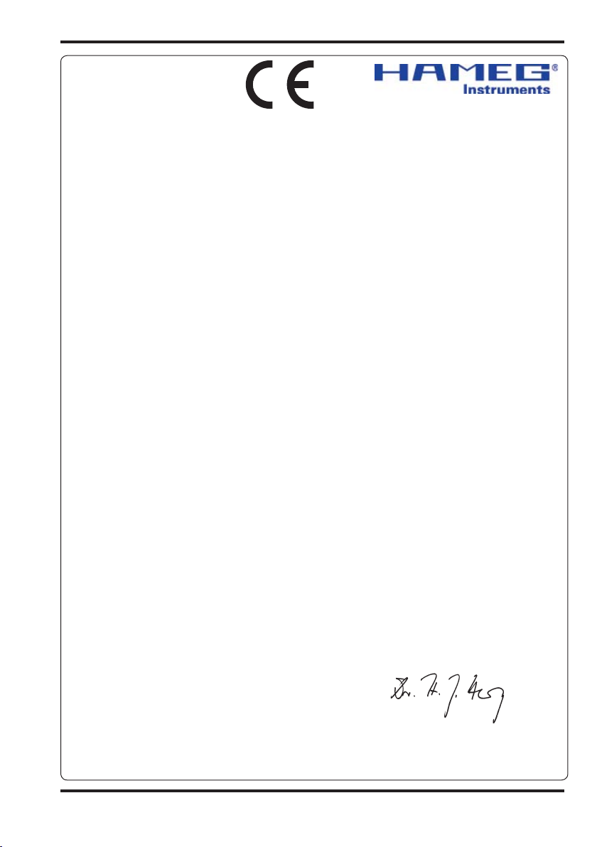
Lieferumfang: Transportkoffer

1 H-Feld Sonde 1 E-Feld Sonde 1 Hochimpedanzsonde 1 BNC-BNC Kabel 1 Spannungsversorgungskabel

Typischer Frequenzverlauf Hochimpedanz Sonde

Batterien (Typ Mignon) gehören

nicht zum Lieferumfang

SCALE = 10dB/DIV.

Typischer Frequenzverlauf E-Feld-Sonde Typischer Frequenzverlauf H-Feld-Sonde

Änderungen vorbehalten / Reservado el derecho de modificación

Der HZ530-Sondensatz besteht aus drei aktiven Breitbandsonden für die EMV-Diagnose bei der Entwicklung elektronischer Baugruppen und Geräte auf Laborebene. Er enthält eine aktive Magnetfeldsonde (H-Feld-Sonde), einen aktiven E-Feld-Monopol und eine aktive Hochimpedanzsonde. Die Sonden sind zum Anschluß an einen Spektrum-Analyzer vorgesehen und haben daher einen koaxialen Ausgang mit einem Wellenwiderstand von 50 Ω.

H-Feld Sonde

Die H-Feld-Sonde gibt einen der magnetischen Wechsel-Feldstärke proportionalen Pegel ab. Mit ihr können Störquellen in elektronischen Baugruppen relativ eng lokalisiert werden und Abschirmungen auf „undichte“ Stellen untersucht werden.

E-Feld Sonde

Der E-Feld-Monopol wird z.B. verwendet, um die Wirkung von Abschirmmaßnahmen zu prüfen. Mit ihm kann auch die Gesamtwirkung von Filtermaßnahmen beurteilt werden, soweit sie etwa das Gerätegehäuse verlassende Kabel und Leitungen betreffen. Ferner kann man mit dem E-Feld-Monopol Relativmessungen zu Abnahmeprotokollen durchführen.

High-Impedanz Sonde

Die Hochimpedanzsonde ermöglicht eine Untersuchung des Störpegels auf einzelnen Kontakten oder Leiterbahnen. Sie belastet den zu prüfenden Meßpunkt mit nur 2pF. Dadurch kann direkt in der Schaltung gemessen werden, ohne nennenswerte Veränderungen der Verhältnisse durch den Meßeingriff.

Allgemeines

Die Sonden haben je nach Typ eine Bandbreite von 100kHz bis über 1000MHz. Sie sind in modernster Technologie aufgebaut, und GaAsFET sowie monolitische integrierte Mikrowellen Schaltungen (MMIC) sorgen für Rauscharmut, hohe Verstärkung und Empfindlichkeit. Der Anschluß der Sonden an Spektrumanalysator, Meßempfänger oder Oszilloskop erfolgt über ein ca. 1,5m langes BNCKoaxial Kabel. Die in den Sonden schon eingebauten Vorverstärker (Verstärkung ca. 30 dB) erübrigen den Einsatz von externen Zusatzgeräten.

Die Sonden werden entweder durch einsetzbare Batterien/Akkus betrieben oder können direkt aus dem HAMEG Spektrumanalysator HM5010 mit Spannung versorgt werden. Die schlanke Bauform erlaubt guten Zugang zur zu prüfenden Schaltung auch in beengter Prüfumgebung. Mittels eines Akkusatzes hat jede Sonde eine Betriebsdauer von ca. 20 - 30 Stunden.

Änderungen vorbehalten / Subject to change without notice

Bedienungsanleitung

Allgemeines

Sofort nach dem Auspacken sollten die Sonden auf mechanische Beschädigungen und lose Teile im Innern überprüft werden. Falls ein Transportschaden vorliegt, ist sofort der Lieferant zu informieren. Die Sonden dürfen dann nicht in Betrieb gesetzt werden.

Symbole

Sicherheit

Die Sonden haben das Werk in sicherheitstechnisch einwandfreiem Zustand verlassen. Sie entsprechen damit auch den Bestimmungen der europäischen Norm EN 61010-1 bzw. der internationalen Norm IEC 1010-1. Um diesen Zustand zu erhalten und einen gefahrlosen Betrieb sicherzustellen, muß der Anwender die Hinweise und Warnvermerke beachten, die in dieser Bedienungsanleitung, im Testplan und in der Service-Anleitung enthalten sind.

Wenn anzunehmen ist daß ein gefahrloser Betrieb nicht mehr möglich ist, so ist so sind die Sonden außer Betrieb zu setzen und gegen unabsichtlichen Betrieb zu sichern. Diese Annahme ist berechtigt,

Bedienungsanleitung beachten

Hochspannung

Erde

• wenn die Sonden sichtbare Beschädigungen hat,

• wenn die Sonden lose Teile enthalten,

• wenn die Sonden nicht mehr arbeiten,

• nach längerer Lagerung unter ungünstigen Verhältnissen (z.B. im Freien oder in feuchten Räumen),

• nach schweren Transportbeanspruchungen (z.B. mit einer Verpackung, die nicht den Mindestbedin gungen von Post, Bahn oder Spedition entsprach).

Änderungen vorbehalten / Reservado el derecho de modificación

Betriebsbedingungen

Der zulässige Umgebungstemperaturbereich während des Betriebs reicht von +10°C... +40°C. Während der Lagerung oder des Transports darf die Temperatur zwischen -40°C und +70°C betragen. Hat sich während des Transports oder der Lagerung Kondenswasser gebildet, müssen die Sonden ca. 2 Stunden akklimatisiert werden, bevor sie in Betrieb genommen werden. Die Sonden sind zum Gebrauch in sauberen, trockenen Räumen bestimmt. Die Betriebslage ist beliebig.

Gewährleistung

Jede Sonde durchläuft vor dem Verlassen der Produktion einen Qualitätstest.

Dennoch ist es möglich, daß ein Bauteil erst nach längerer Betriebsdauer ausfällt. Daher wird auf alle Sonden eine Funktionsgewähr- leistung von 2 Jahren gewährt. Voraussetzung ist, daß im Gerät keine Veränderungen vorgenommen wurden. Für Versendungen per Post, Bahn oder Spedition wird empfohlen, die Originalverpakkung zu verwenden. Transport- oder sonstige Schäden, verursacht durch grobe Fahrlässigkeit, werden von der Gewährleistung nicht erfaßt. Bei einer Beanstandung sollte man am Gehäuse der Sonde eine stichwortartige Fehlerbeschreibung anbringen. Wenn dabei gleich der Name und die Telefon-Nr. (Vorwahl und Ruf- bzw. Durchwahl-Nr. oder Abteilungs bezeichnung) für evtl. Rückfragen angegeben wird, dient dies einer beschleunigten Abwicklung.

Änderungen vorbehalten / Subject to change without notice

Grundlagen der Meßtechnik mit Nahfeldmeßsonden

Die H-Feld-Sonde

Die H-Feld-Sonde gibt einen der magnetischen Wechsel-Feldstärke proportionalen Pegel an das angeschlossene Meßsystem ab. Mit ihr können Störquellen in elektronischen Baugruppen relativ eng lokalisiert werden. Dies hat seine Ursache darin, daß moderne elektronische Baugruppen als Störer meist niederohmig wirken (relativ kleine Spannungsänderungen bei entsprechend großen Stromänderungen). Die abgestrahlten Störungen beginnen daher an ihrer Quelle zunächst überwiegend mit einem magnetischen Wechselfeld. Da beim Übergang vom Nah- zum Fernfeld das Verhältnis vom magnetischen zum elektrischen Feld die 377 0hm Wellenwiderstand des freien Raumes erreichen muß, nimmt das HFeld zunächst mit der dritten Potenz des Abstandes vom Störer ab. Eine Verdoppelung des Abstandes bedeutet ein Abnehmen des Feldes auf ein Achtel.

Beim praktischen Gebrauch der H-Feld-Sonde bemerkt man deshalb ein sehr starkes Ansteigen des Pegels bei Annäherung an den Störer. Beim Absuchen einer Baugruppe mit der H-Feld-Sonde fallen die Störer daher sofort auf. Es kann z.B. schnell festgestellt werden, welcher IC stark stört und welcher nicht. Ferner kann hierbei auf einem Spektrumanalysator erkannt werden, wie sich die Störleistung über den Frequenzbereich verteilt. Somit kann man Bauelemente, die aus EMV-Gründen weniger geeignet sind, schon früh in der Entwicklung eliminieren. Die Wirkung von Gegenmaßnahmen läßt sich qualitativ gut beurteilen. Man kann Abschirmungen auf „undichte“ Stellen untersuchen, und Kabel oder Leitungen auf mitgeführte Störleistungen absuchen.

Die Hochimpedanzsonde

Die Hochimpedanzsonde ermöglicht eine Untersuchung des Störpegels auf einzelnen Kontakten oder Leiterbahnen. Sie ist sehr hochohmig (Isolationswiderstand des Leiterplattenmaterials) und belastet den zu prüfenden Meßpunkt mit nur 2pF. Dadurch kann direkt in der Schaltung gemessen werden, ohne nennenswerte Veränderungen der Verhältnisse durch den Meßeingriff.

Änderungen vorbehalten / Reservado el derecho de modificación

Es kann z.B. die Wirkung von Filter- und Abblockmaßnahmen quantitativ gemessen werden. Es können einzelne Anschlüsse von IC’s als Störer identifiziert werden. Innerhalb von Leiterplatten können problematische Leiterbahnen ermittelt werden. Mit dieser Sonde kann man jeden einzelnen Punkt einer Schaltung direkt dem Spektrumanalysator zugänglich machen. Die niedrige Eingangskapazität und der flache Amplitudenverlauf der Hochimpedanzsonde macht sie auch hervorragend zur Meßung von Frequenzen und Signalanteilen bis in den GHz-Bereich mittels eines Oszilloskopes nutzbar. Die geringe Belastung wird unter Anderem durch Einsatz eines kapazitiven Spannungteilers am Eingang der Sonde und den nachfolgenden Verstärker erreicht. Trotz des eingebauten Verstäkers hat die Sonde jedoch eine Abschwächung von ca. 30dB auf.

Der E-Feld-Monopol

Der E-Feld-Monopol hat von allen drei Sonden die höchste Empfindlichkeit. Er ist so empfindlich, daß man ihn ohne weiteres als Antenne zum Radio- oder Fernsehempfang benutzen könnte. Daher kann man mit ihm die Gesamtabstrahlung einer Baugruppe oder eines Gerätes beurteilen.

Er wird z.B. verwendet, um die Wirkung von Abschirmmaßnahmen zu prüfen. Mit ihm kann auch die Gesamtwirkung von Filtermaßnahmen beurteilt werden, soweit sie etwa das Gerätegehäuse vorlassende Kabel und Leitungen betreffen, und damit die Gesamtabstrahlung beeinflussen. Ferner kann man mit dem E-Feld-Monopol Relativmessungen zu Abnahmeprotokollen durchführen. Dies macht es möglich, erforderliche Nachbesserungen so gezielt auszuführen, daß man bei der Abnahmeprüfung nicht ein zweites Mal durchfällt. Ferner können Abnahmeprüfungen so gut vorbereitet werden, daß man im allgemeinen vor Überraschungen sicher ist.

Inbetriebnahme

Vor Beginn der ersten Messung mit den Sonden HZ530 sind die Hochimpedanzsonde und die E-Feld-Sonde mit den notwendigen Antennen zu versehen. Diese befinden sich in Form von ca. 0.8mm starken, geraden Drähten in einem kleinen Plastikbeutel im Transportkoffer des Sondensatzes. Das Einstecken der Antennen erfolgt mittels einer Zange und unter Anwendung von sanfter Gewalt. Die

Änderungen vorbehalten / Subject to change without notice

Öffnung zur Aufnahme der Antenne befindet sich jeweils im verjüngten vorderen Teil der Sonde. Die kurze Tastspitze ist für die Hochimpedanzsonde vorgesehen. Die zwei längeren Antennen werden für die E-Feld-Sonde verwendet. Je nach vorgesehenem Frequenzbereich kommt die kürzere (ca. 6.5cm) oder längere (9.5cm) Antenne zum Einsatz.

Anschließend wird die Spannungsversorgung der Sonden sichergestellt. Beim Einsatz eines HM5010/5011 kann dies direkt, mittels des mitgelieferten Spezialkabels, aus dem Spektrumanalysator geschehen. Batterien sind dann nicht erforderlich. Wird ein anderer Spektrumanalysator, ein Oszilloskop oder ein Meßempfänger für die Messungen verwendet, so erfolgt die Versorgung durch 4 Mignon-Zellen entweder in Form von Batterien oder entsprechender wiederaufladbarer Akkus.

Zu Beginn der Messung ist die jeweils verwendete Sonde mittels des neben dem BNC-Anschluß befindlichen Schalters in Betrieb zu nehmen. Dies ist unabhängig davon ob die Sonde durch Batterien oder den Spektrum-Analysator versorgt wird. Auf jeden Fall sollte man bei Verwendung von Batterien bei Nichtgebrauch der Sonden die Spannungsversorgung abschalten. Im Normalfall hat ein Satz Batterien eine Lebensdauer von ca. 20-30 Stunden.

Der Anschluß der Sonden an Spektrumanalysator, Meßempfänger oder Oszilloskop erfolgt durch ein mitgeliefertes BNC-Kabel von ca.

1.5m Läge. Dies ermöglicht im Allgemeinen genügend Spielraum

für die notwendigen Messungen. Sollte aus besonderen Gründen ein längeres Kabel verwendet werden, sind Abweichungen des Amplitudenganges bei höheren Frequenzen möglich.

Im Normalfall werden die Sonden in Verbindung mit einem Spektrumanalysator betrieben. Diese Geräte besitzen üblicherweise eine Eingangsimpedanz von 50 ter Abschluß der Sonden gewährleistet. Wird ein Oszilloskop oder ein Messempfänger mit abweichendem Eingangswiderstand angeschlossen, so ist unbedingt auf korrekten Abschluß der Sonden zu achten. Ansonsten ergeben sich erhebliche, nicht abschätzbare Beeinflussungen des Frequenzganges.

Die Sonden sind auf Grund Ihrer elektrischen Charakteristika für unterschiedliche Prüfungen vorgesehen. Die E-Feld-Sonde wird im

Änderungen vorbehalten / Reservado el derecho de modificación

ΩΩ

Ω

. Dadurch ist ein korrek-

ΩΩ

Allgemeinen für Messungen im Abstand von 1m bis 1.5m vom zu untersuchenden Objekt eingesetzt. Die dabei ermittelten Störfrequenzen lassen sich mit der H-Feld-Sonde im Nahbereich der Störquelle lokalisieren. Die Hochimpedanzsonde ermöglicht anschließend die exakte Eingrenzung der Störquelle und die gezielte Beurteilung der getroffenen Maßnahmen.

Die E-Feld-Sonde ist auf Grund Ihrer Eigenschaften nicht für Messungen innerhalb eines Gerätes oder direkt an spannungsführenden Teilen einer Schaltung vorgesehen. Elektrischer Kontakt der Antenne mit spannungsführenden Schaltungsteilen (DC max. 20V; AC max. +10dBm) kann zur Zerstörung des eingebauten Vorverstärkers führen. Die genannten Grenzwerte gelten auch für die Hochimpedanzsonde, hier ist jedoch elektrischer Kontakt für die Messung im Rahmen der vorgegebenen Grenzwerte vorgesehen.

Sicherheitshinweis!

Grundsätzlich ist die Messung an spannungsführenden Schaltungsteilen mit Spannungen höher als 40V mit den Sonden nicht zulässig. Da zu einem erheblichen Teil am geöffneten Gerät gemessen wird, ist Voraussetzung, daß der Benutzer mit den dabei auftretenden Gefahren vertraut ist. Netzbetriebene Geräte müssen bei der Messung über einen Sicherheitstrenntransformator galvanisch vom Netz getrennt werden (erdfrei) .

Es sei in diesem Zusammenhang darauf hingewiesen, daß mit den Sonden keine quantitativen Messungen durchgeführt werden können. Eine auf den Meßergebnissen direkt beruhende Berechnung der Störstrahlung zur Verwendung bei Abnahmeuntersuchungen ist nicht möglich. Der Sondensatz ist als Hilfsmittel zur qualitativen Erfassung von Störfrequenzen im Rahmen von entwicklungsbegleitenden Messungen entwickelt worden. Die Aussagekraft der erzielten Meßergebnisse ist stark von den jeweiligen Randbedingungen der Messungen abhängig. Denken auch Sie an unsere Umwelt. Zur Spannungsversorgung der Sonden sollten Sie möglichst das mitgelieferte Versorgungskabel einsetzen. Ist dies nicht möglich, sollten wiederaufladbare Akkus verwendet werden. Bei der Verwendung von Batterien stellen Sie bitte die sachgerechte Entsorgung sicher.

Änderungen vorbehalten / Subject to change without notice

Applikationen für die Nahfeldsonden HZ 530

Praxisorientierte Auswahl von Signalleitungsfiltern

Die durch die ständig steigende Arbeitsgeschwindigkeit moderner Digitallogik überproportional wachsenden EMV-Probleme werden seit dem 01.01.1996 allen Anbietern elektrischer und elektronischer Produkte drastisch vor Augen geführt. Die neue Gesetzgebung verschärft zwar nicht die Störstrahlungsproblematik, macht aber die Auseinandersetzung mit diesen Gegebenheiten zur Pflicht für jeden Entwickler.

Die Zeiten, in denen man die Lösung der Störstrahlungsproblematik einfach der EMV-Abteilung überlassen konnte, oder ein Produkt, welches nicht direkt durch Störstrahlungsprobleme auffiel unter EMV-Gesichtspunkten als quasi in Ordnung einstufte, sind längst vorbei. Jeder Entwickler muß heute schon vom Beginn des Entwurfs an EMV-Gesichtspunkte mitverfolgen, wenn später bei der Abnahme ein Erfolg überhaupt möglich sein soll. Leiterplatten müssen heute anders entworfen werden als noch vor wenigen Jahren. Eine vernünftige Breitbandentkopplung der Versorgungsspannung muß schon als Stand der Technik angesehen werden.

Aber auch der Bereich der Signalleitungen kann nicht mehr so bleiben wie früher. Digitale Signale haben Spektren, deren Bandbreite ungefähr

entspricht. Die Flankenzeit tr ist also der bestimmende Faktor. Je kürzer die Flankenzeit, desto größer die Bandbreite. Hierbei ist nicht die tabellarisch angegebene Bandbreite entscheidend, sondern nur die tatsächlich vorhandene. Diese kann sich von der angegebenen sehr erheblich unterscheiden. Das hat seinen Grund darin, daß der tabellarische Wert sich meistens auf kapazitive Vollast bezieht. In den meisten praktischen Fällen liegt diese Last aber nicht vor. Eine überschlägige Umrechnung ist recht einfach: Halbe kapazitive Last bedeutet doppelte Flankengeschwindigkeit.

Ein Beispiel möge dies verdeutlichen: ein Mikroprozessor ist mit 2ns Anstiegszeit der Flanke angegeben. Die zugrunde gelegte Last

Änderungen vorbehalten / Reservado el derecho de modificación

B = 1/(tr •

π)

ist 150pF. Wenn nun ein Signal dieses Prozessors mit nur einem CMOS-Gatter, also ca. 12,5pF, belastet wird, heißt dies, daß die Flanke etwa zwölfmal schneller wird. Es muß ein Wert von unter 200ps erwartet werden. Rechnet man dies in die entsprechende Bandbreite des Spektrums um, so erhält man 1,6GHz. Auch in praktischen Aufbauten, in denen noch etwas Schaltungskapazität hinzukommt, kann man tatsächlich Bandbreiten von über 1000MHz messen.

Unter EMV-Gesichtspunkten betrachtet ist dies natürlich äußerst schädlich. Die tatsächliche Flankengeschwindigkeit kann man aber auch bei modernen CMOS - Schaltungen in den meisten digitaltechnischen Labors nicht messen. Hierfür müßten Oszilloskope bereitstehen, die Zeiten von 100ps auflösen können. Diese sind jedoch nur zu sehr hohen Kosten erhältlich.

Für die Auflösung der digitalen Systemfunktionen braucht man diese Geschwindigkeit auch nicht, weshalb in den o.g. Labors meist wesentlich langsamere Geräte verwendet werden. Diese täuschen dem Benutzer Flankenzeiten vor, die in Wirklichkeit nicht existieren. Im allgemeinen sieht man nur die Anstiegszeit des Oszilloskops.

Dies legt ein meßtechnisches Problem offen: Die für die Beurteilung der EMV-relevanten Eigenschaften des Systems erforderlichen Messungen sind mit der existierenden Ausrüstung meist nicht möglich, erforderliche Oszilloskope aber sehr teuer.

Eine brauchbare Lösung besteht im Ausweichen in den Frequenzbereich: Die Beurteilung der digitalen Funktion geschieht weiterhin mit einem mittelschnellen Oszilloskop, die Untersuchung der EMVrelevanten Eigenschaften im Frequenzbereich mittels eines Spektrumanalysators. Da die Spektrum-Analyse entsprechender Frequenzbereiche technisch einfacher ist als die Auflösung im Zeitbereich, sind Geräte welche die Grundvoraussetzungen erfüllen schon vergleichsweise preisgünstig erhältlich. Für die Beurteilung von CMOS - Schaltungen reicht eine Bandbreite von 1000MHz. Entsprechende Oszilloskope sind sehr teuer.

Da Spektrumanalysator hochfrequenztechnische Geräte sind, haben sie üblicherweise einen 50Ω Eingang. Dies macht sie zur Messung in Digitalschaltungen ungeeignet, weil der Anschluß

Änderungen vorbehalten / Subject to change without notice

einer solchen Last in der Regel von der Schaltung nicht verkraftet wird. Zumindest würde das Meßergebnis stark verfälscht. Deshalb benötigt man für die Messung in Digitalschaltungen eine Hochimpedanz-Sonde, die das Meßobjekt nicht nennenswert belastet und das Signal breitbandig auf 50Ω umsetzt.

Im Prinzip könnte man auf den Gedanken kommen, Signalleitungsfilter nach Katalog auszusuchen. Namhafte Hersteller bieten zu ihren Filtern die entsprechenden Meßergebnisse in Zeit- und Frequenzbereich in ihren Katalogen an. Leider sind diese Messungen in der Regel in bezug auf eine ohmsche Last vorgenommen worden. Sie sehen dann auch immer recht gut aus. In der Praxis der Digitalelektronik liegt eine solche Last selten vor. Deshalb kann die verbindliche Beurteilung der Wirkung der Filter nur im realen Anwendungsfall gemessen werden. Es zeigt sich dann, daß die Filter nicht immer die erwarteten Ergebnisse erbringen.

Dies soll im folgenden an einer Reihe von Beispielen, die alle an der Logikfamilie 74ACT gemessen wurden, gezeigt werden. Die Gatter wurden stets mit 5MHz Takt betrieben.

SCALE = 10dB/DIV.

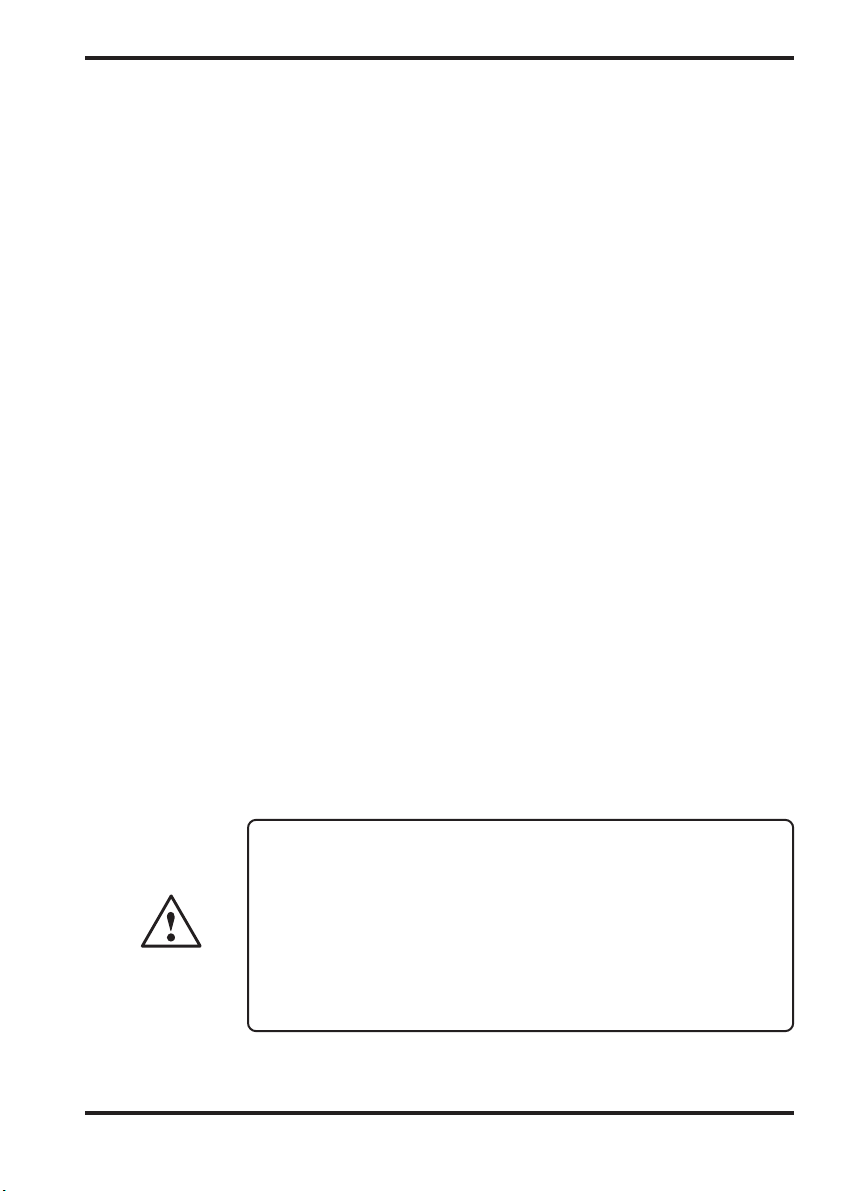
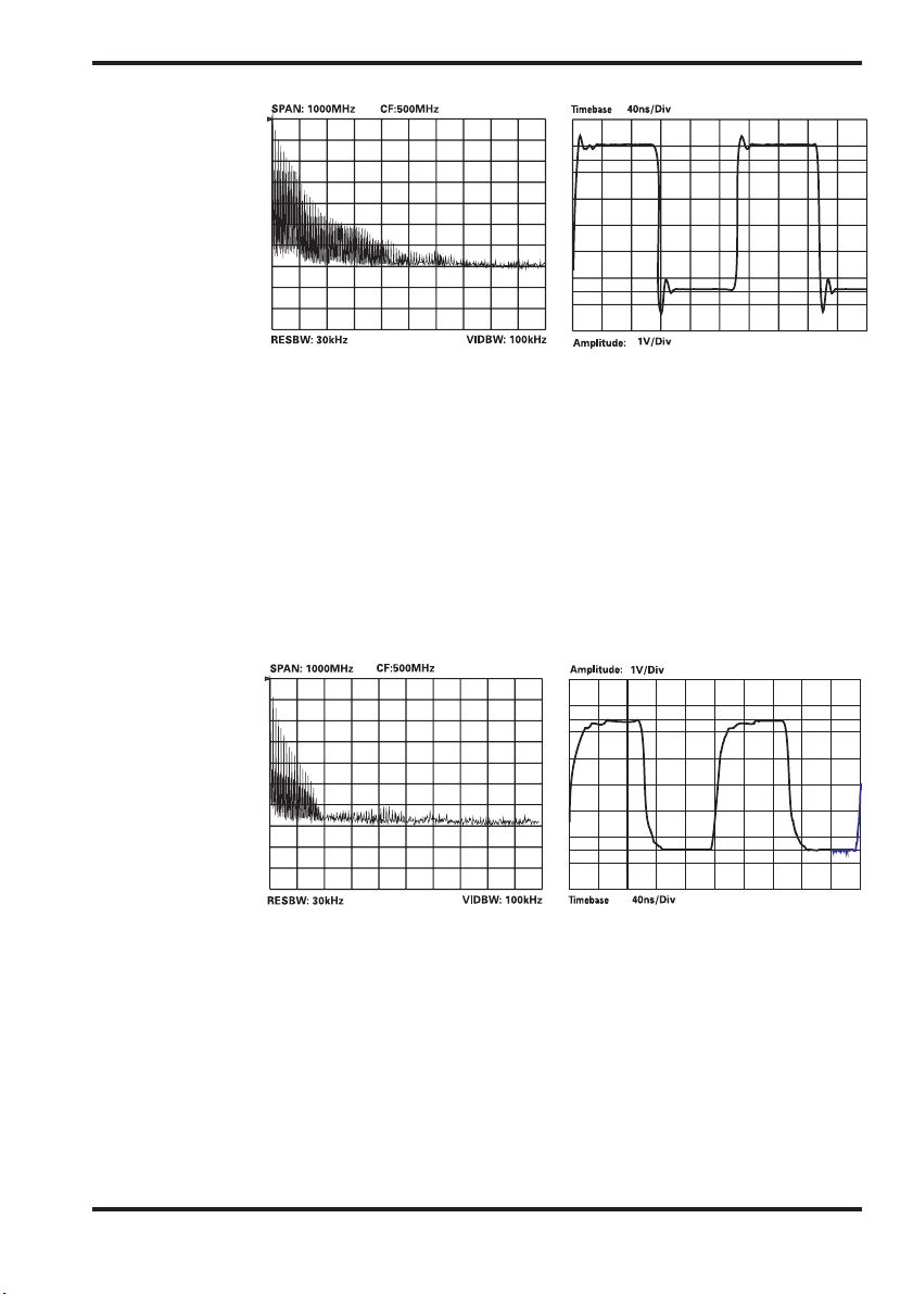
Bild 1 zeigt die Ergebnisse an einem solchen Gatter, welches auf einer Leiterplatte bestückt ist und dessen Ausgang im Leerlauf arbeitet. Das Spektrum deckt den gesamten Bereich bis 1000MHz ab. Tatsächlich reicht es noch darüber hinaus, aber die Spektren in den vorliegenden Bildern sind alle bis 1000MHz skaliert, um einen besseren Vergleich zu ermöglichen. Im Zeitbereich zeigen sich relativ starke Über- und Unterschwinger sowie steile Flanken. Das Signal ist in Bezug auf die EMV als sehr ungünstig einzustufen. Die hohe Bandbreite ermöglicht Abstrahlung schon aus relativ kleinen

Änderungen vorbehalten / Reservado el derecho de modificación

Leiterplatten. Insbesondere, wenn Signale Leiterplatten verlassen sollen, wird die Eingrenzung solcher Spektren unerläßlich, will man nicht erhebliche Abschirmmaßnahmen treffen.

Eine erste Maßnahme in dieser Richtung, die häufig empfohlen wird, ist das Einfügen eines Widerstandes zwischen Gatterausgang und Leitung. Die Leitung ist bei dieser Messung durch einen einzelnen Gattereingang abgeschlossen, um realistische Verhältnisse zu haben. Der Abschluß und auch die Leitungslänge müssen bei solchen Messungen immer den Verhältnissen entsprechen, die im tatsächlichen Anwendungsfall auch vorliegen, weil die Wirkung der Signalleitungsfilter stark von deren Abschluß beeinträchtigt wird.

SCALE = 10dB/DIV.

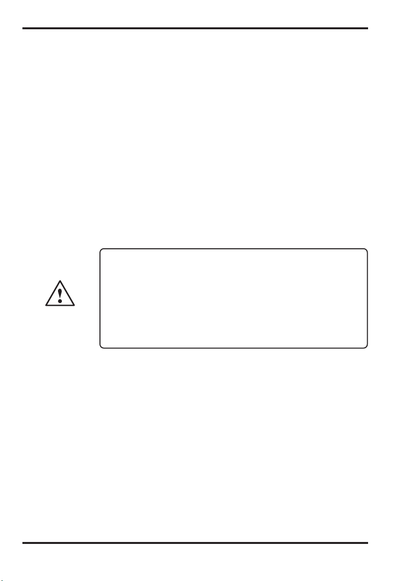
Bild 2 zeigt die entsprechenden Ergebnisse für einen 47Ω Wider- stand. Im Zeitbereich erkennt man eine deutliche Verbesserung: Die Überschwinger sind gemindert, die Flanken weniger steil. Leider täuscht das Ergebnis. Die geringe Dynamik der linearen Darstellung des Oszilloskops kann die EMV-relevanten Eigenschaften des Signals nicht richtig darstellen. Das Spektrum zeigt nur eine sehr geringe Dämpfung oberer Frequenzbereiche. Zum Teil ist an der Täuschung auch der Tastkopf des Oszilloskops beteiligt, da er immerhin mehr als 6pF kapazitive Last mitbringt. Die HochimpedanzSonde weist dagegen nur eine Belastungskapazität von 2pF auf. Mit der Auswahl des Widerstandswertes kann man an dem vorliegenden Ergebnis noch einiges ändern, aber ein durchschlagender Erfolg kann von einer so einfachen Maßnahme, wie sie das Einfügen des Widerstands darstellt, nicht erwartet werden.

Eine weitere Verbesserung läßt sich erzielen, wenn man den Widerstand mit einem Kondensator zu einem RC-Glied ergänzt.

Änderungen vorbehalten / Subject to change without notice

SCALE = 10dB/DIV.

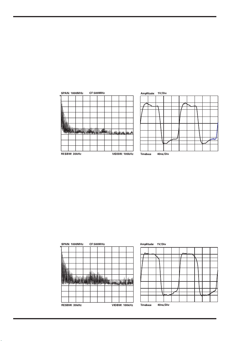
Bild 3 zeigt die Resultate für eine Bestückung mit 47Ω und 100pF. Auch hier erfolgt die Belastung des Aufbaus, wie bisher, mit der Leiterbahn und dem einzelnen Gattereingang. Im Zeitbereich ist im Vergleich zu Bild 2 kaum eine Veränderung erkennbar. Der Frequenzbereich zeigt aber besonders im mittleren und oberen Abschnitt eine deutliche Verbesserung. Besonders bei der Verwendung eines langsameren Oszilloskops würde die Veränderung im Zeitbereich überhaupt nicht mehr wahrnehmbar sein. Hier zeigt sich sehr deutlich die Schwäche einer reinen Zeitbereichsmessung: Man übersieht die EMV-Relevanz der Maßnahme.

SCALE = 10dB/DIV.

Bild 4

Der nächste Schritt besteht in dem Ausbau des Signalleitungsfilters zu einem R-C-R-Glied. Es wurde mit 47Ω, 100pF und 47Ω bestückt. Die Veränderung in Bezug zum vorherigen Zustand ist massiv. Der Frequenzbereich ist praktisch auf 200MHz eingeschränkt. Allerdings ist im Zeitbereich auch ein langsamer Verlauf der Flanke erkennbar. Hier muß die Frage gestellt werden, ob die logische Funktionalität der Digitalschaltung durch eine solche Flanke bereits beeinträchtigt wird. Man kann in einem solchen Falle aber durch

Änderungen vorbehalten / Reservado el derecho de modificación

eine entsprechende Anpassung der Bestückung des R-C-R-Gliedes den günstigsten Kompromiß zwischen Eingrenzung des Spektrums und der logischen Funktionalität aufsuchen. Dies ist ein besonders schönes Beispiel für die Wirksamkeit des hier vorgeschlagenen meßtechnischen Verfahrens.

Im Handel sind verschiedene komplette Signalleitungsfilter im Angebot. Auch die Wirksamkeit dieser Filter läßt sich meßtechnisch in der gleichen Weise verifizieren.

SCALE = 10dB/DIV.

Bild 5 zeigt den Einsatz eines Dreipol - Kondensators als Signalleitungsfilter in dem Aufbau, der auch bei den anderen Messungen verwendet wurde. Das Ergebnis ist enttäuschend: Trotz starker Verlangsamung der Flanken des Signals, ist das Spektrum mangelhaft eingegrenzt. Dies hängt damit zusammen, daß der Masseanschluß solcher Dreipol - Kondensatoren oftmals nicht so induktionsarm ausführbar ist, wie der eines R-C-R-Gliedes in SMD - Technik. Es werden sogar Dreipol - Kondensatoren angeboten, die in diesem Bereich fehlkonstruiert sind. Als weiteres Beispiel soll eine einzelne Breitband - Chip - Drossel als Signalleitungsfilter dienen.

SCALE = 10dB/DIV.

Änderungen vorbehalten / Subject to change without notice

In Bild 6 ist das Resultat zu sehen: Auch hier eine mangelhafte Begrenzung des Spektrums trotz starker Verlangsamung der Flanken. Man beachte: Hier würde eine ausschließliche Betrachtung des Zeitbereichs leicht zu völlig falschen Schlüssen führen: Eine teure Maßnahme, welche die digitale Funktion bereits erheblich belastet, mit enttäuschendem Ergebnis auf der Seite der EMV.

SCALE = 10dB/DIV.

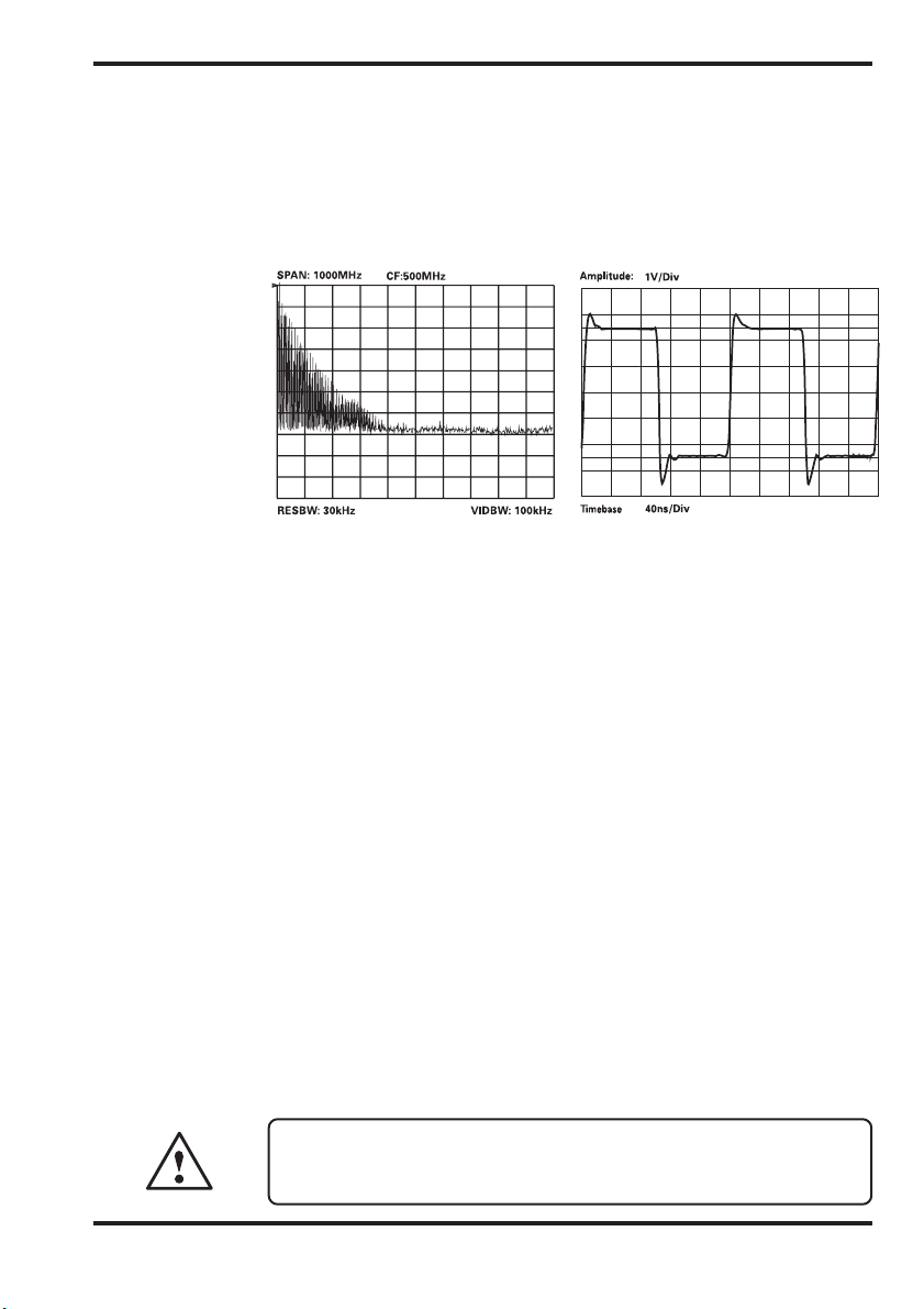
Bild 7

Schlußendlich soll einer der modernen SMD - Chip - Filter, die aus zwei Ferritperlen und einem Durchführungskondensator bestehen, betrachtet werden. Das Ergebnis, das in Bild 7 dargestellt ist, erscheint als recht gut. Das Spektrum ist sauber begrenzt, die Flanken sind noch erstaunlich steil. Lediglich die Über- und Unterschwinger trüben das sonst so gute Bild. Das ist leider ein Problem, das Filter begleitet, die neben kapazitiven auch induktive Komponenten aufweisen. Zusammenfassend kann festgestellt werden, daß für den Digitalelektroniker, der für EMV - Probleme bereits sensibilisiert ist, der Einblick in den Frequenzbereich eine unerläßliche Maßnahme ist, da die reine Betrachtung des Zeitbereichs leicht Anlaß zu Täuschungen gibt. Theoretisch ist zwar alles in der Darstellung im Zeitbereich enthalten, was im Frequenzbereich nur anders beschrieben wird. Die praktisch verfügbaren Meßgeräte lösen dies aber nur unvollkommen auf. Insbesondere die schwache Dynamik der linearen Darstellung im Oszilloskop und die oftmals zu geringe Geschwindigkeit desselben stehen dem Erreichen der theoretischen optimalen Lösung entgegen.

Für die in dieser Applikation dargestellten Meßergebnisse der Freqenzspektren diente die Hochimpedanz-Sonde aus dem Nahfeld-Sondensatz HZ530 als Aufnehmer.

Änderungen vorbehalten / Reservado el derecho de modificación

Messung der Schirmdämpfung von Abschirmgehäusen mit der E-Feld-Sonde

Was bringt es, wenn ich das ganze Gerät in ein Abschirmgehäuse stecke? Das wird sich mancher fragen, der bei der Abnahme zur CE-Zertifizierung durchgefallen ist. Leider kann man die Frage nicht pauschal beantworten, denn nicht jedes metallische Gehäuse schirmt auch gut ab. Kaum einer wird aber bis zur nächsten Abnahmemessung warten wollen. Was, wenn es wieder nicht stimmt? Es ist also erforderlich, ein einfaches Meßverfahren zu haben, mit dem man zunächst den relativen Erfolg beurteilen kann. Hierzu bieten sich hochempfindlichen E-Feld-Sonden an. Man kann sie auch als sehr breitbandige Meßantennen verwenden wodurch sie zur Klärung der o.g. Fragen gut dienen können.

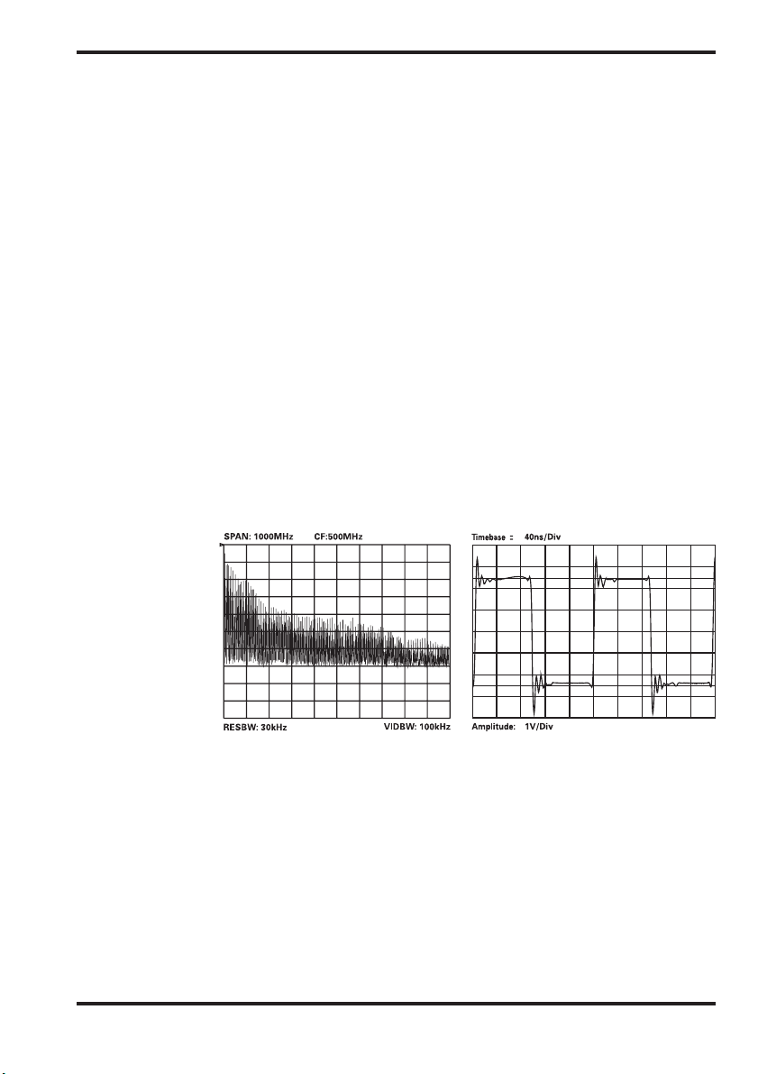
Zunächst muß vor der Verwendung der Sonde geklärt werden, ob sie ausreichend empfindlich ist. Grundsätzlich sind alle passiven Sonden meist unbrauchbar, weil sie zu unempfindlich sind. Die für den Praktiker einfachste Lösung zur Klärung dieser Frage ist die Aufnahme eines Breitbandspektrums von 0 bis 1000MHz in seinem Labor. Bild1 zeigt eine solche Aufnahme, die mittels aktiven E-Sonde aus dem HZ530 Sondensatz aufgenommen wurde. Im Bereich bis 50MHz zeigt sie relativ sehr hohe Pegel die von Rundfunksendern aus dem Mittel- und Kurzwellenbereich stammen. Im Bereich um 100MHz sieht man Signale von UKWRundfunksendern aus der Umgebung. Da es in diesem Fall keinen Ortssender am Platz der Aufnahme gibt fallen diese Signale etwas schwächer aus. Die stärkste Linie 474MHz stammt von einem Fernsehsender, der exponiert in ca. 15km Entfernung steht. Es folgen bis 800MHz mehrere Linien von Fernsehsendern aus der Umgebung. Den Abschluß bildet der Bereich knapp über 900MHz, der zu den örtlichen D-Netz-Stationen gehört. Die Aufnahme zeigt, daß die verwendete Sonde breitbandig und empfindlich ist. Beginnend vom Mittelwellenbereich bis zum DNetz sind Linien zu finden, die weit aus dem Rauschen herausreichen. Natürlich fällt dieses Bild an jedem Ort anders aus, aber da Deutschland überall mit Rundfunk und Fernsehen versorgt ist dürften die zugehörigen Linien nirgendwo fehlen. Auch in sehr ländlichen Bereichen darf heute auch nirgendwo das D-Netz in der Aufnahme fehlen: Es würde zeigen, daß die Sonde eine zu niedrige Grenzfrequenz hat.

Änderungen vorbehalten / Subject to change without notice

HintergrundSpektrum

SPAN: 1000MHz CF:500MHz

Bild 8

SCALE = 10dB/DIV.

RESBW: 10kHz VIDBW: 10kHz

Die Aufnahme des Hintergrundspektrums dient allerdings nicht nur der Prüfung der Sondenempfindlichkeit. Sie soll im Falle, daß man die folgenden Messungen nicht in der Schirmkabine ausführen kann als Referenz dienen, um die wichtigsten Spektrallinien erkennen zu können die nicht aus der zu untersuchenden Elektronik stammen.

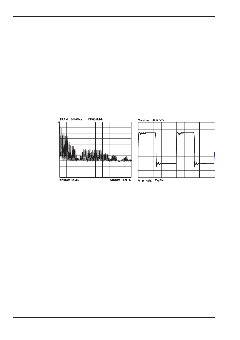
SPAN: 1000MHz CF:500MHz

Störer ohne Abschirmung

Bild 9

SCALE = 10dB/DIV.

RESBW: 10kHz VIDBW: 10kHz

Zur Durchführung der Messung stellt man nun den Prüfling zunächst ohne Abschirmung in einer Entfernung von mindestens 0,5m von der Sonde auf. Dann dreht man den Prüfling, bis man die Richtung des Abstrahlungsmaximums gefunden hat. In dieser Position wird die zweite Aufnahme gemacht (Bild 9). Man erkennt, daß im Vergleich zum Hintergrundspektrum Störleistung bis 1GHz vorhanden ist.

Das Maximum der Störstrahlung liegt im Bereich 250...350MHz. Die stärkste Linie ist mit dem Marker gekennzeichnet, der relative Pegel liegt bei –42.8dBm. Es folgt die zweite Messung: Hierbei trägt der Prüfling sein Abschirmgehäuse. Er wird zuerst so gedreht, daß wieder das Maximum der Störstrahlung gefunden wird. Dieses kann in einer anderen Richtung liegen als bei offenem Gerät.

Änderungen vorbehalten / Reservado el derecho de modificación

Störer mit Abschirmung

SPAN: 1000MHz CF:500MHz

Bild 10

SCALE = 10dB/DIV.

RESBW: 10kHz VIDBW: 10kHz

Bild 10 zeigt das Resultat. Man sieht, daß die Abstrahlung im gesamten Frequenzbereich geringer geworden ist. Aus den Pegeldifferenzen aus Bild 2 und Bild 3 kann die Schirmdämpfung für verschiedene Frequenzen ermittelt werden. Für die markierte Linien entnimmt man: –55,9dbm. Das ergibt eine Dämpfung von 13,1dB. Für Frequenzen bei 800MHz werden nur 9db erreicht. Schirmdämpfungen in dieser Größenordnung scheinen kaum das Blech wert zu sein, aber leider ist so ein Ergebnis nicht ungewöhnlich. Die Messungen wurden an einem handelsüblichen Frequenzzähler der unteren Preisklasse vorgenommen. Es gibt zahllose Geräte, deren Gehäuse keine besseren Werte erwarten lassen. Es lohnt sich also zu messen, bevor man zuviel Geld für Blech ausgibt.

Auch hier zeigt sich wieder die ausgezeichnete Verwendbarkeit der Meßsonden in der entwicklungsbegleitenden EMV-Meßtechnik.

Änderungen vorbehalten / Subject to change without notice

Operating instruction . ...............................................................24

Near Field Sniffer Probes HZ 530 ................................................. 24

Specifications ................................................................................ 24

General Information ....................................................................... 26

Safety ............................................................................................. 26

Operating Conditions ..................................................................... 27

Warranty ........................................................................................ 27

Introduction ...................................................................................28

Operation of the Probes ................................................................29

Battery Operation .......................................................................... 29

Output Impedance Matching ........................................................29

Use of different probe types ......................................................... 30

Safety Notice ................................................................................. 30

Accuracy Notice............................................................................. 31

Basis for Near-Field Probe Measurements ................................... 31

The H-Field Near-Field Probe ........................................................ 31

The High-Impedance Probe ........................................................... 32

The E-Field Monopole Probe ......................................................... 32

HZ 530 Near-Field Probe Applications .......................................... 33

Practical Selection of Signal-Line Filters ....................................... 33

Measurement of the Shielding Attenuation of .............................39

Shielded Housings with the E-Field Probe .................................. 39

Commonly asked questions about

pre-compliance emissions testing . ..........................................41

How can pre-compliance instruments be defined? ................ 42

Why is there such a cost difference between ....................... 42

compliance and pre-compliance test instruments? ................ 42

How important is EMC training? ............................................. 43

How important is an instrument’s amplitude accuracy? ........ 43

Should pre-compliance instruments

contain “CISPR bandwidths”? ................................................ 43

How will the level of ambient signals affect my radiated emissions measurements and will using fully

compliant measuring equipment help? ................................... 43

Will a screened room overcome

the problem of ambient signals?............................................. 44

Can I make meaningful radiated emissions measurements

with a near field probe instead of an antenna? ...................... 44

Do spectrum analyzers have any

advantages over receivers? .................................................... 45

Will a spectrum analyzer allow me to make

sensible emissions measurements?....................................... 45

Does a spectrum analyzer’s response to pulsed

interference influence the measurement result? ...................45

What are the results if I surround the entire

equipment under test in a shielded housing?......................... 46

Does the E-Field-Monopole of the HZ530 have

sufficient sensitivity for pre-compliance testing? ................... 46

Table of contents

Änderungen vorbehalten / Reservado el derecho de modificación

Near Field Sniffer Probes HZ 530

Specifications

Frequency range: 0.1MHz to 1000MHz

(lower frequency limit depends on probe type)

Output impedance: 50Ω Output connector: BNC-jack Input capacitance: 2pF

Max. Input Level: +10dBm

1dB-compression point: -2dBm

(frequency range dependent)

DC-input voltage: 20V max. Supply Voltage: 6V DC

Supply Current: 8mA (H-Field Probe)

Probe Dimensions: Housing: Plastic;

(electrically shielded internally)

(high imped. probe)

(without destruction)

4 AA size batteries Supply-power of HM5010/5011

15mA (E-FieldProbe) 24mA(High imp.Probe) 40x19x195mm (WxDxL)

Package contents: Carrying case

1 H-Field Probe 1 E-Field Probe 1 High Impedance

Probe

1 BNC cable (1.5m)

1 Power Supply Cable (Batteries or Ni-Cads are not included)

SCALE = 10dB/DIV.

Frequency Response High Impedance Probe (typical)

SCALE = 10dB/DIV.

Frequency Response H-Field Probe (typical)Frequency Response E-Field Probe (typical)

Änderungen vorbehalten / Subject to change without notice

The HZ530 is the ideal toolkit for the investigation of RF electromagnetic fields. It is indispensable for EMI pre-compliance testing during product development, prior to third party testing.

The set includes 3 hand-held probes with a built-in pre-amplifier covering the frequency range from 100kHz to over 1000 MHz.

The probes - one magnetic field probe, one electric field probe, and one high impedance probe - are all matched to the 50Ω inputs of spectrum analyzers or RF-receivers. The power can be supplied either from batteries, Ni-Cads or through a power cord directly connected to an HM5010/11 series spectrum analyzer.

Signal feed is via a 1.5m BNC-cable. When used in conjuction with a spectrum analyzer or a measuring receiver, the probes can be used to locate and qualify EMI sources, as well as evaluate EMC problems at the breadboard and prototype level. They enable the user to evaluate radiated fields and perform shield effectiveness comparisons. Mechanical screening performance and immunity tests on cables and components are easily performed.

The H-Field Probe

The magnetic probe incorporates a high degree of rejection of both stray and direct electric fields, and provides far greater repeatability than with conventional field probes. Measurements can be made on the very near field area that is close to components or radiation sources. It is especially suited to locate emission “hot spots” on PCBs and cables.

The E-Field Probe

The electric field (mono-pole) probe has the highest sensitivity of all three probes. It can be used to check screening and perform pre-

compliance testing on a comparative basis.

High Impedance Probe

The high impedance probe is used to measure directly on the components under test or at the conductive trace of a PC board. It has an input capacitance of only 2pF and supplies virtually no electrical charge to the device under test.

Änderungen vorbehalten / Reservado el derecho de modificación

General Information

Users are advised to read through these instructions so that all functions are understood. Immediately after unpacking, the instrument should be checked for mechanical damage and loose parts in the interior. If there is transport damage, the supplier must be informed immediately. The probes must then not be put into operation.

Symbols

Safety

The probes have been designed and tested in accordance with

Publication 1010-1, Safety requirements for electrical equipment for measurement, control, and laboratory use

regulations EN 61010-1 correspond to this standard. They have left the factory in a safe condition. This instruction manual contains important information and warnings which have to be followed by the user to ensure safe operation and to retain the probes in a safe condition.

ATTENTION - refer to manual

Danger - High voltage

Protective ground (earth) terminal

IEC

. The CENELEC

Whenever it is likely that protection has been impaired, the instrument shall be made inoperative and be secured against any unintended operation. The protection is likely to be impaired if, for example, the instrument

• shows visible damage,

• fails to perform the intended measurements,

• has been subjected to prolonged storage under unfavourable conditions (e.g. in the open or in moist environments),

• has been subject to severe transport stress (e.g. in poor packaging).

Änderungen vorbehalten / Subject to change without notice

Operating Conditions

The probes have been designed for indoor use. The permissible ambient temperature range during operation is +10°C (+50°F) ... +40°C (+104°F). It may occasionally be subjected to temperatures between +10°C (+50°F) and -10°C (+14°F) without degrading its safety. The permissible ambient temperature range for storage or transportation is -40°C (+14°F) ... +70°C (+158°F). The maximum relative humidity is up to 80%.

If condensed water exists in a probe it should be acclimatized before switching on. In some cases (e.g. probe extremely cold) two hours should be allowed before the probe is put into operation.

Warranty

Specifications:

Values without tolerances are typical for an

average instrument.

HAMEG warrants to its Customers that the products it manufactures and sells will be free from defects in materials and workmaship for

period of 2 years

a failure or damage caused by improper use or inadequate maintenance and care. HAMEG shall not be obliged to provide service under this warranty to repair damage resulting from attempts by personnel other than HAMEG representatives to install, repair, service or modify these products.

In order to obtain service under this warranty, the Customer must contact and notify the distributor who has sold the product.

Each probe is subjected to a quality test before leaving the production. In case of shipments by post, rail or carrier it is recommended that the original packing is carefully preserved. Transport damages and damage due to gross negligence are not covered by this warranty.

In case of a complaint, a label should be attached to the probe which describes briefly the faults observed. Indicating the name and telephone number (dialing code and telephone or direct number or department designation) will help speeding up the processing of warranty claims.

. This warranty shall not apply to any defect,

Änderungen vorbehalten / Reservado el derecho de modificación

Introduction

Electromagnetic compatibility continues to be an important issue in the electronics industry worldwide. The main goal of design engineers is to meet even more demanding specifications, while also making circuitry quieter and more robust to meet tough EMC regulations. The design of microcontroller-based products which fully comply with present and imminent EMC regulations isn’t an easy task to undertake with the use of current technologies. Even with the best PCB layout techniques and the most substantial decoupling, at the speeds of today’s designs, radiation from boards and the consequent noise impinging on PCBs is becoming a growing problem that will not go away.

By the date of January 1, 1996, every electronic instrument or device which can be imported to the European community must meet the EMC regulations according to EN 55011 to 22 , EN 500811 and CISPR-Publications 11 to 22. The EMC directive refers to both electromagnetic emissions and electromagnetic immunity. The manufacturer of electronic equipment or devices declares the conformity of his product with the above regulations by the placement the CE-sign on the device or equipment. By doing so the manufacturer is liable for all violations of the above regulations. Goods without the CE-sign are not allowed to be sold in the European Community.

In order to be sure that the manufactured equipment meets all specifications according to the EMC regulations, extensive test during the design phase of every electronic device must be done. One of the methods of CE certification is to use the services of a professional testing lab that specializes in the compliance certification process. The lab will have precise test equipment and a shielded, screen room within which the inspection is performed. Since many products being certified will require modification and redesign, the customer is charged on an hourly basis for test time used. Quite often, many trips are made between the test lab and the design/development facility. In order to minimize the cost of the test, it is recommended that a “Pre-Compliance” phase in product development first be conducted. This phase would use a spectrum analyzer such as the HM5010 in conjunction with HZ 530 close field sniffer probes, to inspect for emission and leakage; isolate the source, design and correct the problem and then retest.

Änderungen vorbehalten / Subject to change without notice

Once the product appears electromagnetically “quiet”, it is submitted to the compliance certification laboratory. This should save the expense for much of the test time, since the submitted unit has already been pretested. Typically, the test time and money saved should represent many times the purchase price of the spectrum analyzer.

Operation of the Probes

Before performing measurements with two of the HZ 530 probes, the High Impedance (Hi-Z) Probe and the E-Field Probe they must be configured for testing. The 0.8 mm diameter wires which are used as antennas are located in the plastic bag that is in the case for the probes. The wires are plugged into the probe by use of pliers and a light force. The opening for the antenna is located on the narrower front of the probes. The short wire is intended as a contact for the Hi-Z probe. The two longer antennas are to be used on the E-field probe. Depending on the frequency range either the short antenna (6.5cm) or the long antenna (9.5cm) is used.

Battery Operation

Next, power must be provided to the probes. If a HM 5010 spectrum analyzer is used, the necessary voltage is obtained from the HM 5010 by use of a provided special cable. In this case, batteries are not required. If another spectrum analyzer, oscilloscope or RFI measurement set is used for the measurement, the supply must be provided via 4 AA-Cells either NiCad or rechargeable batteries.

Prior to each measurement the switch needs to be actuated. This switch is located adjacent to the BNC connector. This switch must be turned on when either the battery or spectrum analyzer supply are used. However, when not in use, the switch must be turned off to save the batteries which have a life of 20 - 30 hours when turned on.

Output Impedance Matching

The connection of the probe to the spectrum analyzer, oscilloscope or measurement receiver is made via a supplied BNC cable of approximately 1.5 meters length. This length is generally sufficient

Änderungen vorbehalten / Reservado el derecho de modificación

for most measurements. If for special reasons a longer cable is used, the insertion loss of this cable must be added to the output values at the higher frequencies.

For the normal measurements, the probes are connected to a spectrum analyzer. These instruments generally have an input impedance of 50 impedance for the probes. If an oscilloscope or measurement receiver with a different impedance is used, the correct (50 termination impedance must be used. If the 50 impedance is not used, the probe output is not calibrated.

Use of different probe types

The different probes are used for different tests since their electric characteristics are quite different. The E-field probe is normally used at a distance of 0.5 to 1.5meters from the RFI source. The thereby observed frequencies are then further localized near the source by use of the H-field probe. The high impedance (Hi-Z) probe makes further localization possible by directly contacting the source and to judge the effectiveness of suppression measures.

Because of its electrical characteristics, the E-field probe is not intended to perform measurements within an equipment or directly on parts that are live. Electrical contact of the antenna with live parts exceeding 20 VDC or + 10 dBm at RF may cause damage to the built-in pre-amplifier. These limits also apply to the Hi-Z probe; however, electrical contact to parts that are below 20VDC or + 10dBm are permitted.

ΩΩ

Ω

s. This impedance is the normal termination

ΩΩ

Ω

termination

ΩΩ

Ω

)

ΩΩ

Safety Notice

Basically, it is not permissible to perform measurements on parts that are live above 40V. Since a significant part of the measurements are performed on exposed parts, it is a prerequisite that the user is familiar with any potential electrical hazard. Under no circumstances may the probes be used on equipment that is not safety grounded. When in doubt, a safety isolation transformer must be used.

Think also of ecology. The power supply for the probes should be,

Änderungen vorbehalten / Subject to change without notice

whenever possible, be made by use of the supplied 1.5 m supply cable connected to the spectrum analyzer. If this is not possible, rechargeable batteries should be used. If non-rechargeable batteries are used, they should be disposed of properly.

Accuracy Notice

The probes may not be used to perform accurate quantitative measurements. It is not possible to relate the probe measurements directly to final values of field strength in V/m necessary for certification tests. The probe kit is intended as an aid for developmental tests to obtain a qualitative amplitude as a function of frequency. These values are strongly influenced by the limiting conditions of the measurement which may change as a function of frequency.

Basis for Near-Field Probe Measurements The H-Field Near-Field Probe

The H-Field probe provides a voltage to the connected measurement system which is proportional to the magnetic radio frequency (RF) field strength existing at the probe location. With this probe, circuit RF sources may be localized in close proximity of each other. This effect is caused by the interference sources which in modern electronic circuits are of low resistance (relatively small changes in voltage cause large changes in current). The sources of radiated interference begin as a primarily magnetic radio frequency field ( HField) directly at its origin. Since in the transition from the near- to the far-field, the relationship between the magnetic- to the far-field must reach the free-space impedance of 377Ω, the H-field will decrease as the cube of the distance from the source. A doubling of the distance will reduce the H-field by a factor of eight (H = 1/d³); where d is the distance.

In the actual use of the H-field sensor one observes therefore a rapid increase of the probe’s output voltage as the interference source is approached. While investigating a circuit board, the sources are immediately obvious. It is easily noticed which (e.g.) IC causes interference and which does not. In addition, by use of a spectrum analyzer, the maximum amplitude as a function of frequency is easily identified. Therefore one can eliminate early in

Änderungen vorbehalten / Reservado el derecho de modificación

the development components which are not suitable for EMC purposes. The effectiveness of countermeasures can be judged easily. One can investigate shields for “leaking” areas and cables or wires for conducted interference.

The High-Impedance Probe

The high-impedance probe (Hi-Z) permits the determination of the radio frequency interference (RFI) on individual contacts or printed circuit traces. It is a direct-contact probe. The probe is of very high impedance (near the insulation resistance of the printed circuit material) and is loading the test point with only 2pF (80Ω at 1GHz). Thereby one can measure directly in a circuit without significantly influencing the relationships in the circuit with the probe.

One can, for example, measure the quantitative effectiveness of filters or other blocking measures. Individual pins of IC’s can be identified as RFI sources. On printed circuit boards, individual problem tracks can be identified. With this Hi-Z probe individual test points of a circuit can be connected to the 50Ω impedance of a spectrum analyzer.

The E-Field Monopole Probe

The E-field monopole probe has the highest sensitivity of the three probes. It is sensitive enough to be used as an antenna for radio or TV reception. With this probe the entire radiation from a circuit or an equipment can be measured.

It is used, for example, to determine the effectiveness of shielding measures. With this probe, the entire effectiveness of filters can be measured by measuring the RFI which is conducted along cables that leave the equipment and may influence the total radiation. In addition, the E-field probe may be used to perform relative measurements for certification tests. This makes it possible to apply remedial suppression measures so that any requalification results will be positive. In addition, pre-testing for certification tests may be performed so that no surprises are encountered during the certification tests.

Änderungen vorbehalten / Subject to change without notice

HZ 530 Near-Field Probe Applications Practical Selection of Signal-Line Filters

The steadily increasing operating speed of modern digital logic causes significantly greater concerns with EMC problems. This has become more noticed by all manufacturers of electrical and electronic devices since 1 January l996, the effective compliance date for the European Union EMC Directive. The EMC Directive does not cause the radiated interference problems, but it causes conflict with the requirements of compliance for each manufacturer.

The times are long gone when the EMC problems could be left to the EMC department or a non-compliant product was not noticed and could be sold anyhow. Every circuit designer must at the beginning of a development be aware of potential EMC problems to even allow the successful certification of a product. Printed circuit boards must be built differently than was possible several years ago. A reasonable broadband decoupling of the supply voltages is the present state-of-the-art. But also the design of signal lines must be considered and can not be left to chance. Digital signals have a spectrum with a bandwidth, B, that is related by:

B = 1 / (3.14 • tr), where tr is the risetime.

Consequently, the risetime of a digital signal transition is the determinant. The shorter the risetime, the wider the frequency range. However, the calculated bandwidth is not as important as the one that actually exists which can be significantly different than the calculated one. The reason for this is that the calculated value is referenced to a capacitive total load. For most practical cases this does not occur. An approximate calculation shows that one half of the capacitive load means a twice faster risetime; e.g. a microprocessor has a specified risetime of 2 x 10E-9 s (2ns). The capacitive load is supposed to be 150 pF. If a signal from this processor is loaded only with a CMOS gate of 12.5 pF, the risetime will be 12 times faster and a value of 200 x 10E-12 s (200ps) must be expected. In the frequency domain, 200ps is equivalent to a bandwidth of 1.6GHz. Even in practical circuits, where additional capacitance can be expected, actual bandwidths of over 1GHz are measurable.

Änderungen vorbehalten / Reservado el derecho de modificación

From an EMC point of view, this is naturally very damaging. The actual risetime in CMOS circuits is not easily measurable in most digital labs. To measure the actual risetimes, oscilloscopes with the ability to measure 100ps (10E-10s) must be used. Such oscilloscopes are available but at a significant price.

Such fast oscilloscopes are not really necessary to observe the digital system operation. This is the reason that these fast oscilloscopes are not used in digital laboratories and slower oscilloscopes are used. However, slow scopes simulate a risetime which in reality do not exist because they measure only the internal risetimes of the oscilloscope.

This exposes a measurement problem: The relevant EMC characteristics cannot be measured with existing equipment in many cases and the necessary oscilloscope is very expensive.

A practical solution is to perform the measurements in the frequency domain: The digital function is observed with a slower and economical oscilloscope and the relevant EMC characteristics are measured with a spectrum analyzer. Since the spectrum analysis of corresponding frequency ranges is technically simpler than the measurement of the equivalent risetimes, basic spectrum equipment can be obtained which is relatively more economical. Spectrum analyzers with a bandwidth of 1,000MHz are already suitable for analyzing CMOS circuits. The corresponding oscilloscopes are still very expensive.

Spectrum analyzers are high frequency equipment and have therefore an input impedance of 50Ω. They are therefore not suitable to measure directly in digital circuits because of this impedance which will influence the circuit behavior. As a minimum the measurement results are false. Consequently, for the measurement in digital circuits a high impedance probe is required which does not load the circuit and convert the signal to a 50Ω system over a wide frequency range.

The following measurement results were measured with the High Impedance Probe HZ530 connected to a Spectrum Analyzer and with a digital scope.

Änderungen vorbehalten / Subject to change without notice

In principle, it is easy to assume that it is possible to select signalline filters from catalog values. Well-known manufacturers offer filters with measurement data in the time- and frequency- domain. Unfortunately, the filter data is performed with an entirely resistive load and therefore the data looks very good. However, in practice an entirely resistive circuit seldom exists. Therefore, the filters must be evaluated when installed in a practical circuit. It is then observed that the performance of the filters is not as promised in the catalog. This shall be demonstrated with a series of illustrative examples which are measured in circuits of the 74 ACT family. The gates are always operated with a 5MHz frequency.

SCALE = 10dB/DIV.

Figure 1 shows the time and frequency domain outputs of such a gate which is mounted on a printed circuit and is not loaded. The frequency spectrum is measurable to 1,000MHz. In fact, it extends even above 1,000MHz, but for comparison purposes all measurements are scaled only 1,000MHz. In the time domain relatively strong over and under shoot and fast risetimes are observable. This signal is very poor relative to the EMC characteristics. The excessive bandwidth permits radiation to take place on relatively small printed circuit boards. When this signal is conducted to other parts, it is especially important to limit the spectrum to avoid excessive shielding structures.

As a first measure to limit the spectrum, a resistor is recommended between the gate output and the conductor connection. The conductor is simulated by an individual gate input to obtain a realistic circuit. The connection and the conductor length must correspond to the actual relationship to make the measurements of signal line filter evaluation meaningful. The effectiveness of line filters is strongly influenced by their termination.

Änderungen vorbehalten / Reservado el derecho de modificación

SCALE = 10dB/DIV.

Figure 2 shows the results when a 47Ω resistor is used. In the time domain a significant improvement occurs. The overshoot is reduced and the risetimes are somewhat slower. The linear dynamic range of an oscilloscope can not demonstrate adequately the EMC characteristics of the signal. The frequency spectrum shows only a slight decrease of the upper frequencies. The oscilloscope probe is partially responsible for this error since the probe has a capacitance of 6pF. The Hi-Z probe has only a load capacitance of 2pF. By selecting specific values of resistors the EMC characteristics may be slightly improved, but an EMC success can not be scored with only the insertion of a resistor. Another improvement can be made by inserting a capacitor to form an RC filter.

SCALE = 10dB/DIV.

Figure 3 shows the results when 100pF is added to the 47Ω

resistor. The load continues to be the printed circuit track and another gate input. In the time domain, the difference appears negligible. In the frequency domain, the middle and upper frequency range is significantly improved. If a slower oscilloscope is used, any improvement would no longer be recognizable in the time domain. The limitation of using an oscilloscope and using only time domain

Änderungen vorbehalten / Subject to change without notice

measurements is easily recognizable: The EMC relevance of a suppression measure is not noticeable. The next step is to insert a 47Ω, 100 pF, 47Ω T-filter.

SCALE = 10dB/DIV.

Figure 4 shows that the change is quite noticeable when compared to Figure 3. The frequency range is now practically reduced to 200 MHz. At the same time the risetime is significantly slowed down. The approach may be questionable if this slow risetime influences the digital operation. In this case, the component values may be varied to find a compromise between desired EMC characteristics and digital functionality. This suitable example demonstrates the effectiveness of the measurement procedures recommended here.

Several complete signal-line filters are commercially available. The effectiveness of these filters can be evaluated using the same procedures.

SCALE = 10dB/DIV.

Figure 5 shows the use of a three-pole capacitor used as a signalline filter in the same circuit as used in the previous examples. The results are disappointing: Even though the risetime is significantly reduced, the frequency spectrum is only marginally reduced. This

Änderungen vorbehalten / Reservado el derecho de modificación

results from the generally poor ground connection of a three-pole capacitor which is relatively high in inductance compared to a R-CR combination in surface mount technology (SMT). Some offered three-pole capacitors are poor high frequency filters.

Another example is a wideband choke used as a signal line filter.

SCALE = 10dB/DIV.

Figure 6 shows the results. The frequency spectrum is poorly suppressed, but the risetimes are significantly slowed down. It should be noticed here that a time domain analysis only will lead to poor EMC performance and the wrong conclusions. This is an expensive measure that will influence the digital function with disappointing EMC suppression.

As a final example a modern SMT chip filter consisting of two ferrite beads and a feed-through capacitor is shown.

SCALE = 10dB/DIV.

Figure 7 shows the results which are relatively good. The spectrum is limited and the risetime is surprisingly fast. The overand under-shoot is somewhat disappointing. This occurs in filters which consist of only inductance and capacitance.

Änderungen vorbehalten / Subject to change without notice

In conclusion, it is observed that the digital circuit designer who is aware of EMC problems, must look at the frequency domain and not only at the time domain or a false picture may result. Theoretically, everything is contained in the time domain which is only differently presented in the frequency domain. The problem rests with the linear presentation and the resolution of the oscilloscope. Using a generally poor oscilloscope will not lead to a theoretically optimal solution.

Measurement of the Shielding Attenuation of Shielded Housings with the E-Field Probe

What are the results if I surround the entire equipment in a shielded housing? This question will be asked if I fail the CE-Mark EMC test. Unfortunately, this question can not be answered in general because a metallic housing is not always a good shield. No one wants to wait until the next full-scale EMC test for the results. What if the EUT fails again? What is needed is a simple measurement procedure to determine the relative improvement of the radiated RFI. For this purpose the highly sensitive E-Field probe is used, which is used as broad bandwidth measurement antennas to help answer the above questions.

First, before the E-field probe is used, determination must be made if the probe has sufficient sensitivity and bandwidth. In general, all passive probes are not usable since they have insufficient sensitivity. The simplest solution to determine the sensitivity and bandwidth is to measure the existing ambient field in the practitioner’s laboratory that is generated by the surrounding transmitters from 0 to 1,000MHz. Figure 8 shows the result of such a measurement which was made with the active E-field probe from the HZ530 probe kit connected to a spectrum analyzer. From 0 to 50MHz, Figure 8 shows relative high levels which originate from transmitters in the broadcast band and shortwave region. In the frequency range near 100MHz signals from FM stations are noticeable. Since in the particular case measured, there were no nearby FM transmitters, the amplitudes are relatively low. The strongest signal observed was a UHF TV transmitter at 474MHz which was located only 15 km from the laboratory. Then up to 800MHz are several weaker (more distant) UHF TV transmitters. The final signals occur above 900MHz which are related to cellular telephones. This data shows that the probe is wideband and has sufficient sensitivity. From the

Änderungen vorbehalten / Reservado el derecho de modificación

AM band around 1MHz to the cellular telephone band there are spectrum lines which are significantly above the noise level. Of course, the spectrum display will be different at each location depending on the relative distance of transmitters. Even in rural areas cellular telephone lines must show the absence of which would show that the probe has insufficient sensitivity at the higher frequencies.

Measurement of the Ambient Spectrum.

SCALE = 10dB/DIV.

Figure 8

The measurement of the ambient spectrum serves not only to determine probe sensitivity. If the measurements are not performed in a shielded room, the ambient signals can also serve as a reference to recognize the most important frequencies which do not originate from the EUT.

To perform the measurements, the EUT is set up, without the additional shield, at a minimum distance of 0.5 meter from the probe. Then the EUT is rotated in azimuth to find the maximum of the radiation from the EUT. At this point the data is recorded as shown in Figure 9.

EUT RFI Characteristics without Additional Shield

SCALE = 10dB/DIV.

Figure 9

Comparison of Figure 9 with Figure 8 shows that RFI is radiated up to a frequency of 1GHz. The maximum of the radiated power occurs at frequencies between 250 to 350MHz. The strongest signal is at the marker frequency of 275MHz at a level of 42.8 dBm.

Änderungen vorbehalten / Subject to change without notice

Next, the same measurement is performed with the additional shielding around the EUT. Again the EUT must be rotated in azimuth until the maximum RFI is observed. The direction may be different than in the non-shielded equipment.

EUT RFI Characteristics with the Additional Shielding

SCALE = 10dB/DIV.

Figure 10

Figure 10 shows the data with the additional shield. By comparing Figure 10 with Figure 9, it is observed that the entire spectrum is lower. The shielding attenuation can be determined from these two figures. For the marker frequency of 275MHz a signal of -55.9 dBm gives a shielding effectiveness of [-42.8(-)-55.9 dBm] of 13.1 dB. For the frequency of 800MHz, the shielding effectiveness is only 9 dB. Shielding effectiveness of this magnitude are hardly worth the additional sheet metal. But such results are quite common. These measurements were performed on an EUT which was low-price frequency counter. There is other equipment where similar results are obtained because the radiation may also occur from windows and other openings in the housing or cables connected to the EUT. However, it is cost-effective to measure before spending money for sheet metal.

Änderungen vorbehalten / Reservado el derecho de modificación

Commonly asked questions about pre-compliance emissions testing

The EMC Directive has prompted a large selection in the choice of EMC test instruments. In particular, a new class of low-cost precompliance instruments has opened an debate on the merits of this new class of instruments compared with established high-cost EMC compliance test equipment. In this situation it’s not surprising that a high degree of confusion prevails. In order to get a clear view of the situation, the first step is to define compliance and precompliance EMC test equipment and then establish how they differ. HAMEG Instruments has considerable experience with both types of equipment. We use high-cost equipment for compliance testing and also specify and design low-cost pre-compliance equipment. As a result, we are well positioned to express a balanced view in this debate. The following questionnaire is a summary of commonly asked questions concerning the practical use of HAMEG measuring equipment for EMC pre-compliance testing and how useful EMC pre-compliance instruments are in general.

How can pre-compliance instruments be defined?

EMC standards for both radiated and conducted emissions require that compliance measuring equipment conforms to CISPR 16-1. This requirement implies that for full compliance tests you need expensive, high-quality receivers. On the other hand, you can use pre-compliance equipment as tools to build EMC conformance into your products during design and development. Often the debate over compliance or pre-compliance instruments reduces to a choice between a test receiver or a spectrum analyzer. However, these definitions and choices are not the whole story because the way you make EMC measurements can have more influence on the validity of a test than the type of equipment you use.

Why is there such a cost difference between compliance and pre-compliance test instruments?

Instruments for making compliance measurements must conform to CISPR 16. This standard details stringent requirements, and some are costly to implement. Pre-compliance instruments provide

Änderungen vorbehalten / Subject to change without notice

valuable measurements and possess some of the features of compliance equipment. Generally, though, precompliance instruments do not need to conform fully to CISPR 16 and therefore can cost less. Compliance equipment is your first choice if money is no object. In reality, often you cannot justify the cost of such equipment and need a more economical approach. Pre-compliance instruments cost less and can provide useful measurements, but you must be aware of the difference between the two types of equipment and what you get as a measurement result. It is entirely possible to make meaningless measurements with a US$50,000 CISPRcompliant receiver. Equally, you can make valuable measurements with a US$5,000 pre-compliance set-up.

How important is EMC training?

EMC training is vital irrespective of whether you make compliance or pre-compliance measurements. Much of the current debate regarding the two types of instruments is rooted in misconceptions that arise because of lack of knowledge and training. Without proper training you can make meaningless measurements irrespective of the type of equipment you use.

How important is an instrument’s amplitude accuracy?

An instrument’s amplitude accuracy is important, but uncertainty for the whole measurement is of equal importance. If total measurement uncertainty is ±6dB, the additional uncertainty between a ±0.5dB receiver accuracy and a ±2dB spectrum analyzer accuracy is small.

Should pre-compliance instruments contain “CISPR bandwidths”?

The significance of CISPR bandwidths depends if your objective is full compliance or pre-compliance testing. Not all pre-compliance equipment necessarily contains CISPR-compliant bandwidths.

How will the level of ambient signals affect my radiated emissions measurements and will using fully compliant measuring equipment help?

The level of ambient signals that exist in your laboratory or at a particular “open area test site” directly affects your ability to make

Änderungen vorbehalten / Reservado el derecho de modificación

radiated emissions measurements. In some industrial environments, the existing ambient may make obtaining radiated emissions measurements very difficult. There is no advantage in using compliance instruments in such locations.

Will a screened room overcome the problem of ambient signals?

Any Faraday cage structure provides screening from externally generated ambient signals. However, in an unlined screened room, any electromagnetic energy inside from the unit under test, for instance - reflects from all the metallic surfaces of the room. The result is a very uneven and position sensitive field, and you will measure different levels depending on the positions of both the unit and the antenna. You may encounter errors up to ±40dB irrespective of the instruments you use.

Can I make meaningful radiated emissions measurements with a near field probe instead of an antenna?

The two types of measurements are different. In fact, they are complementary and not alternatives. A near field probe only operates in the “near field”, whereas an antenna operates in the “far field”. In the near field you cannot easily quantify the impedance of the source, whereas in the far field the impedance of free space is a constant 377Ω.

For example, a near field probe allows you to detect RF currents on printed circuit boards, and consequently enables you to pin-point problem signals that you first observed using an antenna on an open area test site. If you are going down to detect the source of the radiation (e.g. a transistor, IC, or any other component) on the contact-level, the high-impedance probe of the HZ530 probe set is indispensable for measurements due to its ultra-low input capacitance of 2pF only.

Do spectrum analyzers have any advantages over receivers?

Yes. Spectrum analyzers are generally more flexible, particularly for design and diagnostic testing. The main advantage is that you can observe large frequency spans, whereas a receiver only displays one amplitude and one frequency at a time. An additional

Änderungen vorbehalten / Subject to change without notice

advantage of the HM5000 Spectrum Analyzer series is its fast sweep rate. The display is “updated” every 23ms which allows very fast tracking of the test signal.

Will a spectrum analyzer allow me to make sensible emissions measurements?

The main problem with noise floor occurs when you make radiated emissions measurements. Radiated emissions limits for residential, commercial, or light industrial environments with a 10-meter separation between a unit under test and an antenna are 30 to 230 MHz for 30 dB uV/m, and 230 to 1000 MHz for 37 dB uV/m. A typical maximum receiver noise floor is 1-5 dB uV, whereas for a spectrum analyzer the noise floor is around 10-20 dB uV. Clearly, sensible measurements at some frequencies are not easily obtained with a spectrum analyzer because the noise floor is comparable with the limit.

You can overcome this limitation by using a 3-meter test distance, or by use of a pre-selector or preamplifier (which is built-in for example in the E-Field probe of the HZ530) with the spectrum analyzer. Each of these methods effectively increases the limit or reduces the noise floor of the measurement.

On the other hand we observed in many cases clearly noticeable radiation from the test receiver or measuring equipment itself. Concerning this phenomena the HM 5000 series spectrum analyzer has a big advantage due to its strictly analog design. There is no self generated radiation measurable from the analyzer within its own sensitivity range.

Does a spectrum analyzer’s response to pulsed interference influence the measurement result?

CISPR 16 contains a curve that defines how quasi-peak detectors respond to a pulsed signal. The curve is based upon the signal’s pulse repetition frequency (PRF). For a 30MHz to 1000MHz radiated emissions measurement, the measured value of the input signal can potentially be reduced by a figure up to about 40dB. This number is also known as the overload factor. The design of a compliance receiver ensures this response. However, pulsed

Änderungen vorbehalten / Reservado el derecho de modificación

signals can overload a spectrum analyzer’s input circuitry, particularly on signals with a very low PRF. In practice, few signals have such a low PRF and therefore errors occur infrequently.

What are the results if I surround the entire equipment under test in a shielded housing?

This question is often asked if a CE-Mark EMC test is failed. Unfortunately, this question can not be answered in general because a metallic housing is not always a good shield. No one wants to wait until the next full-scale EMC test for the results. What if the EUT fails again? What is needed is a simple measurement procedure to determine the relative improvement of the radiated RFI. For this purpose the highly sensitive E-Field probe is used, which is used as broad bandwidth measurement antenna to help answer the above questions.

Does the E-Field-Monopole of the HZ530 have sufficient sensitivity for pre-compliance testing?

First, before the E-field probe is used, determination must be made if the probe has sufficient sensitivity and bandwidth. In general, all passive probes are not usable since they have insufficient sensitivity. The E-Field-Monopole is sensitive enough to be used as an antenna for radio or TV reception. With this probe the entire radiation from a circuit or an equipment can be measured.

Änderungen vorbehalten / Subject to change without notice

Conjunto de sondas HZ530

para la diagnosis de EMC ................................48

Sonda de campo H ........................................... 49

Sonda de campo E ............................................ 49

Sonda de alta impedancia ................................. 49

Generalidades ................................................... 49

Instrucciones de manejo .................................. 50

Generalidades ................................................... 50

Símbolos ........................................................... 50

Seguridad ..........................................................50

Condiciones de funcionamiento .......................51

Garantía ............................................................. 51

Principios básicos de la técnica de medida

con sondas de campo cercano ......................... 51

Sonda de campo H ........................................... 51

Sonda de alta impedancia ................................. 52

Sonda monopolo de campo E .......................... 52

Puesta en funcionamiento ................................ 53

Indicación de seguridad ....................................54

Aplicaciones para las sondas

de campo cercano HZ530 ................................. 55

Elección práctica de filtros

de conductos de señal ...................................... 55

Medición de la atenuación de aislamiento

de blindajes mediante la sonda de campo E. ...61

Índice

Änderungen vorbehalten / Reservado el derecho de modificación

Conjunto de sondas HZ530 para la diagnosis de EMC

Datos técnicos Margen de frecuencias:

100kHz - ≥ 1000MHz (frecuencia límite inferior dependiente del tipo de sonda)

Impedancia de salida: 50Ω Conexión: Borne BNC Capacidad de entrada: aprox 2pF

(sonda de alta impedancia)

Nivel de entrada máx.: +10dBm (no deteriorable) Punto de compresión de 1dB:

-2dBm (dependiente de la frecuencia)

Tensión de entrada CC máx.: 20V Tensión de alimentación:

6V CC (Pila o HM5010)

Consumo:

aprox 8mA; sonda campo H aprox.15mA; sonda campo E aprox.24mA; sonda de alta impedancia

Dimensiones de la sonda:

40x19x195 mm (A x Al x L) Caja: Plástico con aislamiento

eléctrico en el interior

Contenido :

Maleta de transporte 1 sonda de campo H 1 sonda de campo E 1 sonda de alta impedancia 1 cable BNC - BNC 1 cable de alimentación

SCALE = 10dB/DIV.

Las pilas (tipo Mignon) no van incluidas en el suministro!

SCALE = 10dB/DIV.

Curva de respuesta de la sonda de campo E

Curva de respuesta de la sonda de alta impedancia

SCALE = 10dB/DIV.

Curva de respuesta de la sonda de campo H

Änderungen vorbehalten / Subject to change without notice

El conjunto de sondas HZ530 se compone de tres sondas activas de banda ancha para la diagnosis de EMC durante el diseño de grupos electrónicos y aparatos. Contiene una sonda activa de campo magnético (sonda campo H), una sonda activa de campo eléctrico de un polo (campo E) y una sonda activa de alta impedancia. Están previstas para ser conectadas a un analizador de espectros y llevan por esta razón una salida coaxial con una impedancia de 50 ohmios.

Sonda de campo H

Sonda de campo E

Sonda de alta impedancia

La sonda de alta impedancia permite la investigación del nivel de ruido sobre los diferentes contactos y circuitos. Sólo carga el punto de medida con 2pF. Gracias a esto se puede medir directamente en el circuito, sin generar variaciones importantes durante la medición.

Generalidades

Todas las sondas tienen un ancho de banda de 100kHz hasta por encima de los 1000MHz. Para su construcción se han utilizado las tecnologías más modernas. Los GaAsFet utilizados así como los circuitos integrados para microondas (MMIC) garantizan un nivel de ruido bajo, una amplificación elevada y alta sensibilidad. La conexión de las sondas al analizador de espectros, receptor de medida u osciloscopio se realiza mediante un cable coaxial BNC de 1,5m de longitud. Los preamplificadores incorporados en las sondas (aprox. 30 dB) hacen innecesario la utilización adicional de aparatos externos, hecho que facilita el manejo considerablemente.

Las sondas se autoalimentan por una pila/batería interna o directamente a través de los analizadores de espectros de HAMEG

Änderungen vorbehalten / Reservado el derecho de modificación

HM5010 y HM5011. Su diseño estilizado permite medir cómodamente el circuito que se desea comprobar, aún con difícil acceso al mismo. Un set de baterías adquirible como opción, suministra una autonomía de trabajo entre 20 a 30 horas. Posteriormente se deberá utilizar adicionalmente un cargador, suministrable como accesorio.

Las sondas se suministran en un conjunto de tres dentro de una maleta robusta y de aspecto profesional.

Instrucciones de manejo Generalidades

Después de desembalar las sondas, compruebe primero que estas no tengan daños externos ni piezas sueltas en su interior. Si muestran daños de transporte, hay que avisar inmediatamente al suministrador o transportista. En tal caso no ponga las sondas en funcionamiento

Símbolos

Atender las instrucciones de manejo

Alta tensión

Masa

Seguridad

Las sondas han salido de fábrica en perfecto estado de seguridad y funcionamiento. Se corresponden con la normativa europea EN 61010 y la norma internacional IEC 1010-1. El manual de instrucciones, el plan de chequeo y las instrucciones de mantenimiento contienen informaciones y advertencias importantes que deberán ser observadas por el usuario para conservar el estado de seguridad de las sondas y garantizar un manejo seguro.

Cuando haya razones para suponer que ya no es posible trabajar con seguridad, hay que apagar el aparato y asegurar que no pueda ser puesto en marcha involuntariamente. Tales razones pueden ser:

• las sondas muestran daños visibles,

• las sondas contienen piezas sueltas,

• las sondas ya no funcionan,

Änderungen vorbehalten / Subject to change without notice

• han pasado un largo tiempo de almacenamiento en condiciones adversas (p.ej. al aire libre o en espacios húmedos),

• su transporte no fue correcto (p.ej. en un embalaje que no correspondía a las condiciones mínimas requeridas por los transportistas).

Condiciones de funcionamiento

El margen de temperatura ambiental admisible durante el funcionamiento va desde +10°C hasta +40°C. La temperatura permitida durante el almacenaje y el transporte es de 40°C hasta +70°C. Si durante el almacenaje se ha producido condensación, habrá que climatizar las sondas durante 2 horas antes de ponerlas en marcha. Las sondas están destinadas para ser utilizadas en espacios limpios y secos. La posición de funcionamiento es a libre elección.

Garantía

Antes de abandonar la producción, todas las sondas se someten a una prueba de calidad. Pero aún así, es posible que algún componente se averíe después de un tiempo de funcionamiento más prolongado. Por esta razón, todas las sondas tienen una garantía de 2 años. La condición es que no se haya efectuado ningún cambio en ellas y se remita el registro de garantía a HAMEG (dirección ver tapa trasera del manual). Se aconseja guardar cuidadosamente el embalaje original para posibles envíos de las sondas por correo, tren o transportista. Los daños de transporte y los daños por grave negligencia no quedan cubiertos por la garantía. En caso de reclamaciones, aconsejamos adjuntar una nota con una breve descripción de la anomalía. Además puede acelerar nuestro servicio si en la mismo nota indica su nombre y número de teléfono (prefijo, número de teléfono y nombre del departamento) para que podamos solicitarle más información respecto a la avería.

Principios básicos de la técnica de medida con sondas de campo cercano

Sonda de campo H

La sonda de campo H suministra al analizador de espectros un nivel proporcional a la intensidad del campo alterno. Esto permite localizar en un margen relativamente estrecho ruidos de grupos electrónicos. El origen está, en que los grupos electrónicos de moderna generación generan ruidos de baja impedancia (variaciones de tensión relativamente pequeñas con variaciones de intensidad

Änderungen vorbehalten / Reservado el derecho de modificación

relativamente altas). Los ruidos emitidos comienzan por esta razón en su origen, con un campo magnético alterno. Como para alcanzar la transición del campo cercano al lejano, se tiene que llegar a la relación de campo magnético/eléctrico de 337 ohmios de resistencia de onda del libre espacio, el campo H se reduce a niveles de la tercera potencia de la distancia de la fuente del ruido. El doble en distancia se corresponde a una reducción del campo a un octavo.

Durante la utilización práctica de la sonda H, se evidencia un fuerte incremento del nivel con la aproximación a la fuente de ruido. Durante el proceso de búsqueda de la fuente de ruido, se detecta por esto rápidamente el componente emisor. Es fácil de comprobar p. ej. cual de los CI está emitiendo un alto grado en ruido y cual no.

Gracias al analizador de espectros se puede reconocer entonces como se distribuye el ruido en el margen de frecuencias. Así es posible, eliminar ya en un estado preliminar del diseño, componentes poco idóneos por razones de compatibilidad electromagnética (EMC). Las contramedidas realizadas se pueden valorar cualitativamente bien. Se pueden analizar los blindajes en busca de puntos “permeables” y controlar cables y conductos eléctricos por ruidos.

Sonda de alta impedancia

La sonda de alta impedancia permite la investigación del nivel de ruido sobre los diferentes contactos y circuitos. Es de muy alta impedancia (resistencia de aislamiento del material de los circuitos) y sólo carga el punto de medida con 2pF. Gracias a esto se puede medir directamente en el circuito, sin generar variaciones importantes durante la medición.

Se puede medir p. ej. la reacción de filtros y de medidas de bloqueo cuantitativamente. Se pueden identificar también las diferentes conexiones de IC como fuentes de ruido. Dentro de la circuitería se pueden localizar las zonas problemáticas. Mediante esta sonda se puede hacer accesible cualquier punto del circuito al analizador de espectros.

Sonda monopolo de campo E

El monopolo de campo E tiene la mayor sensibilidad de las tres sondas. Es tán sensible, que se podría utilizar como antena de recepción de radio o TV. Por esta razón se puede evaluar la emisión total de un grupo electrónico o de un aparato.

Änderungen vorbehalten / Subject to change without notice

Se utiliza para comprobar la eficacia de medidas de aislamiento. También se puede evaluar la eficacia total de filtrado, si corresponden a cables y conductos que se derivan de la carcasa del aparato y que influyen en la irradiación total. Además se pueden realizar mediciones relativas para la documentación de la homologación. Esto permite realizar posteriormente mejoras necesarias tán específicamente, que no se denegará una segunda tramitación a la homologación. Se pueden preparar las homologaciones tan bien, como para asegurarse de sorpresas indeseadas.

Puesta en funcionamiento

Antes de comenzar la medición con las sondas HZ530 se les deben acoplar a la sonda de alta impedancia y a la sonda de campo E las antenas correspondientes. Estas se suministran en una bolsita de plástico que contiene la maleta de transporte y tienen el aspecto de unas varillas de 0,8mm de espesor. Se introducen las antenas mediante unas pinzas - alicate con cierta presión. La abertura en la sonda se encuentra en la parte conificada delantera de la sonda. La antena más corta es para la sonda de alta impedancia. Las dos antenas más largas se utilizan para la sonda de campo E. Según el margen de frecuencia que se desee captar se utiliza la antena de aprox. 6,5cm o la de 9,5cm de longitud.

A continuación se elige el sistema de alimentación para la sonda. Si se utiliza el analizador de espectros HM5010, esta se autoalimenta a través del cable especial de alimentación adjuntado en el suministro. Entonces no se precisan pilas. Si se utiliza otro analizador de espectros al mencionado, entonces se debe realizar la alimentación a través de 4 pilas tipo Mignon o los correspondientes acumuladores recargables.

Antes de efectuar la medición se debe de poner en funcionamiento la sonda mediante el conmutador posicionado al lado del borne BNC. Esto es independiente al sistema de alimentación utilizado. En todo caso es conveniente apagar la sonda si no está en uso. Durante una utilización normal, se dispone de entre 20 y 30 horas de funcionamiento con la alimentación por pilas.

La conexión de las sondas al analizador de espectros, receptor de medida u osciloscopio, se realiza mediante un cable BNC de 1,5m de longitud incluido en el suministro. Esto permite la suficiente movilidad durante las mediciones. Si por alguna razón se utilizara

Änderungen vorbehalten / Reservado el derecho de modificación

un cable de mayor longitud, podría ocasionar variaciones en el margen de la amplitud en frecuencias elevadas.

El caso normal es la utilización de las sondas con un analizador de espectros. Los aparatos tienen normalmente una impedancia de entrada de 50

ΩΩ

Ω

. Entonces se cargan las

ΩΩ

sondas correctamente. Si se conecta un osciloscopio o un receptor de medida con una impedancia de entrada diferente, se debe atender a cargar las sondas con una carga terminal correcta. Sino pueden aparecer influencias inprevisibles en la frecuencia.

Las sondas están previstas para diferentes aplicaciones, según sus características eléctricas. La sonda de campo E se utiliza normalmente para distancias de 1 a 1,5m del objeto a analizar. Las frecuencias perturbadoras se pueden captar con la sonda de campo H en las inmediaciones de la fuente de emisión. La sonda de alta impedancia permite después la circunscripción exacta de la fuente perturbadora y la evaluación precisa de las medidas correctoras realizadas.

La sonda de campo E no es idónea, en base a sus características, para las mediciones dentro de un aparato o directamente en partes de un circuito conectado a una tensión. El contacto directo de la antena con piezas que estén bajo una tensión (DC max 20V; AC max. +10dBm) pueden ocasionar el deterioro del preamplificador de la sonda. Los valores indicados también son válidos para la sonda de alta impedancia, pero el contacto eléctrico para una medición está previsto dentro de los márgenes preestablecidos.

Indicación de seguridad

Por norma, no está permitida la medición con las sondas en piezas de circuitería bajo tensiones superiores a los 40V. Ya que se suelen efectuar muchas mediciones con el aparato abierto, es condición que el operario conozca los riesgos que esto lleva consigo. Bajo ningún concepto es permisible utilizar las sondas en mediciones sin conducto de protección (masa). En otro caso se debe utilizar un transformador separador.

Debemos indicar en este contexto, que no se pueden realizar con las sondas medidas cuantitativas. Un cálculo directo de la

Änderungen vorbehalten / Subject to change without notice

emisión de ruido para la obtención de homologaciones basado en los resultados de la medición no es posible. El conjunto de sondas se ha diseñado para la captación cualitativa de frecuencias perturbantes dentro del marco de mediciones auxiliares de I+D. Los resultados de la medición son muy dependientes de las condiciones marco de cada medida.

Piense en nuestro entorno. Para alimentar las sondas es conveniente utilizar el cable de alimentación especial adjuntado. Si esto no es posible es conveniente utilizar pilas recargables. Si utiliza pilas normales deshéchelas en un contenedor especial.

Aplicaciones para las sondas de campo cercano HZ530

Elección práctica de filtros de conductos de señal

Los problemas en EMC que se ocasionan a través de la velocidad de trabajo creciente de la lógica digital moderna, se constatan drásticamente a los producentes de productos eléctricos y electrónicos desde el 01.01.1996. La nueva legislación no encrudece la problemática de las emisiones, pero sí obliga a ocuparse a los diseñadores del asunto.

Pasaron ya los tiempos en los que se podía dejar en manos del departamento de EMC la solución de los problemas ocasionados por las emisiones, o dejar sin control exhaustivo los productos que no tenían una problemática constatable. Actualmente, los diseñadores deben seguir desde un principio las emisiones posibles del producto, para obtener a su finalización la homologación. Los circuitos impresos deben diseñarse hoy en día de otra forma que hace unos años. Un desacoplamiento adecuado de banda ancha debe tomarse ya como una base de la técnica.

También los conductos de las señales deben modificarse, hoy en día. Las señales digitales tienen espectros, cuyo ancho de banda se corresponde a aprox.: B = 1/(tr * π). El tiempo del flanco tr es el factor determinante. Como más breve sea el tiempo de flanco, más amplio será el ancho de banda. Para esto no es relevante el ancho de banda descrito en la tabla, sino la realmente existente. Esta se puede diferenciar de la descrita sensiblemente. Su razón está, en que el valor de la tabla se refiere bajo carga total capacitativa. En la mayoría de los casos pero, no se da esta carga máxima. Un cálculo

Änderungen vorbehalten / Reservado el derecho de modificación

aproximado se obtiene de forma fácil: Carga capacitativa media corresponde a velocidad de flanco doble.

Un ejemplo dará claridad: un microprocesador se especifica con 2ns de tiempo de subida de flanco. La carga empleada es de 150pF. Si una señal de este µ-procesador se carga con un sólo CMOS de aprox 12,5pF, quiere decir que el flanco se acelera 12 veces. Se debe esperar entonces un valor inferior a los 200ps. Si esto se recalcula en el ancho de banda del espectro, se obtienen 1,6GHz. Diseños prácticos, que incluyen algo más de capacidad por la circuitería, se pueden medir realmente anchos de banda superiores a los 1000MHz.

Bajo aspectos EMC esto es realmente dañino. La velocidad real de flanco pero, en los circuitos con CMOS, no es medible en la mayoría de laboratorios digitales técnicos. Para esto se precisan osciloscopios que puedan presentar señales de 100ps y estos sólo se obtienen en base a un gran desembolso monetario.

Para la resolución de funciones de sistema digitales no es realmente necesaria esa velocidad, por lo que en los laboratorios mencionados anteriormente se suelen encontrar aparatos mucho más lentos. Estos fingen al usuario unos tiempos de flancos que no existen realmente. Generalmente sólo se ve el tiempo de subida del osciloscopio.

Esto revela un problema de técnica de medida: La evaluación de las características relevantes EMC del sistema para las medidas necesarias no se pueden realizar con el equipamiento existente, pero los osciloscopios necesarios son demasiado caros.

Una solución es la separación en el margen de frecuencia: La evaluación de la función digital se realiza mediante un osciloscopio medianamente rápido, mientras que las características relevantes de EMC en frecuencia se obtienen mediante un analizador de espectros. Ya que el análisis de espectros de los correspondientes márgenes de frecuencia es técnicamente más fácil que la resolución en el margen de tiempo, se obtienen estos instrumentos a un coste relativamente bajo. Para la observación de circuitería CMOS es suficiente un ancho de banda de 1000MHz. Los osciloscopios correspondientes son muy caros.

Änderungen vorbehalten / Subject to change without notice

Ya que los analizadores de espectros son instrumentos que incluyen partes de alta frecuencia, llevan normalmente bornes de entrada de 50Ω. Esto les excluye normalmente para las mediciones en circuitería digital, ya que esta no permite cargas de esta magnitud. El resultado de medición quedaría, como mínimo altamente deformado. Por esta razón se necesita, para las mediciones en circuitos digitales, una sonda de alta impedancia, que no carga el circuito a medir y que traspasa la señal en banda ancha a los 50Ω. Los resultados de las mediciones presentadas a continuación se obtuvieron mediante la utilización de un analizador de espectros Anritsu 2601A, así como de un osciloscopio Hewlett-Packard 54502A con sonda HP10430A. Como receptor se utilizó la sonda de alta impedancia del conjunto HZ530.

En principio se podría tener la idea, de seleccionar los filtros en conductos de señal, por catálogo. Hay fabricantes importantes que ofrecen sus filtros en catálogos con las características técnicas correspondientes de medida, en márgenes de tiempo y frecuencia (gráficos). Sin embargo estas mediciones se han realizado en referencia a una carga óhmica. Entonces su visualización queda muy positiva. En la práctica de la electrónica digital no se trabaja normalmente con una carga de estas características. Por esta razón sólo se puede evaluar la respuesta del filtro mediante la prueba real en la práctica y en el circuito. Entonces se detecta, que los filtros no dan los resultados deseados.

Esto se demuestra a continuación en base a unos ejemplos, medidos todos en una familia lógica 74ACT. Las puertas se utilizaron con frecuencias de 5MHz.

SCALE = 10dB/DIV.

Figura 1 muestra los resultados de así una puerta (gate), incorporada en un circuito impreso y cuya salida trabaja sin carga. El espectro

Änderungen vorbehalten / Reservado el derecho de modificación

cubre toda la gama desde 1000MHz. Realmente lo sobrepasa, pero los espectros de las imágenes presentes van con escalas hasta los 1000MHz, para permitir una mejor comparación. En el margen del tiempo se observan variaciones importantes de sobreoscilaciones así como flancos empinados. Esta señal se puede determinar como muy mala respecto a su EMC. Su ancho de banda alto genera una emisión ya desde circuitos impresos relativamente pequeños. Especialmente cuando se pretende que las señales se transmitan a otros circuitos impresos, es imprescindible la limitación de estos espectros, si no se quieren tomar medidas de blindaje elevadas.

Una primera medida que se puede tomar en este caso, sería la incorporación de una resistencia entre la salida de la puerta y el conducto. El conducto queda cerrado en esta medición por una entrada única de puerta, para obtener condiciones reales. La terminación y la longitud del conducto deberán corresponder durante estas mediciones, siempre a las condiciones reales a las que corresponde el caso real, ya que el efecto de los filtros del conducto de la señal dependen en gran medida de su terminación.

SCALE = 10dB/DIV.

Figura 2 muestra los resultados correspondientes para una resistencia de 47Ω. En tiempo se reconoce una mejora notable: las sobreoscilaciones se han reducido y los flancos son menos empinados. Pero el resultado realmente confunde. La pobre dinámica del osciloscopio en la presentación lineal no puede presentar correctamente las características relevantes de EMC. El espectro muestra sólo una atenuación mínima en los márgenes de frecuencia superiores. Parte de la confusión va a cuenta de la sonda del osciloscopio, ya que carga con una capacidad de 6pF. La sonda de alta impedancia en cambio, sólo carga la línea con 2pF. Mediante

Änderungen vorbehalten / Subject to change without notice

la elección del valor de la resistencia se puede modificar en algo el resultado actual, pero la variación no será espectacular. Otra mejora se conseguirá combinando la resistencia mediante un condensador a un conjunto RC.

SCALE = 10dB/DIV.

Figura 3

La figura 3 muestra los resultados de una composición con 47Ω y 100pF. También aquí se carga el circuito mediante el conducto y la entrada única de la puerta. En tiempo no se podrá observar casi diferencia con figura 2. Pero el margen de frecuencias muestra en la zona mediana y superior una mejora contundente. La variación en el tiempo no sería visible si se utilizara aquí un osciloscopio más lento, por lo que se observa claramente las limitaciones de la medición real en tiempo, ya que no se aprecia la relevancia de EMC en las medidas.

SCALE = 10dB/DIV.

Figura 4

El siguiente paso se emprende ampliando el filtro del conducto de la señal mediante un componente R-C-R. Se estableció mediante 47Ω, 100pF y 47Ω. La variación referente al estado anterior es importante. El margen de frecuencia ha quedado limitado a 200MHz. Pero también se observa un flanco más lento. Se debe cuestionar

Änderungen vorbehalten / Reservado el derecho de modificación

en este momento , si la funcionalidad lógica del circuito digital ha sufrido algún perjuicio. Pero en así un caso se puede buscar un compromiso adaptando el componente R-C-R entre la limitación del espectro y la funcionalidad lógica. Este es un buen ejemplo para la eficacia del procedimiento de medición descrito. Se pueden adquirir en el mercado varios filtros completos de conducto de la señal. La eficacia de estos filtros se puede verificar con el procedimiento de medición descrito.

SCALE = 10dB/DIV.

Figura 5

La figura 5 muestra la utilización de un condensador de tres polos, utilizado como filtro de conducto de señal y que ha sido utilizado también en las otras mediciones. El resultado es decepcionante. A pesar de una reducción de los flancos de la señal, el espectro queda insuficientemente delimitado. Esto ocurre porque los condensadores de tres polos no se pueden obtener con una inducción baja como la de los componentes R-C-R en tecnología SMD. Existen hasta condensadores de tres polos, que no están construidos, en este ámbito, correctamente. Como siguiente ejemplo se toma una bobina - chip de banda ancha como filtro de conducto de señal.

SCALE = 10dB/DIV.

Figura 6

Änderungen vorbehalten / Subject to change without notice

En la figura 6 se puede observar el resultado: aquí también aparece una delimitación insuficiente a pesar de la ralentización del flanco. Obsérvese: sería erróneo analizar únicamente el tiempo y sería una medida cara que carga la función digital con resultados decepcionantes en lo que se refiere a EMC.

SCALE = 10dB/DIV.

Figura 7

Finalmente se observará un filtro Chip moderno en SMD, compuesto de dos perlas de ferrita y un condensador de paso. El resultado, visualizado en figura 7, es aceptable. El espectro queda bien delimitado, mientras que los flancos permanecen sorprendentemente empinados. Sólo aparecen los sobreimpulsos y enturbian la buena imagen. Es un problema, que acompaña los filtros que incorporan además de componentes capacitativos también inductivos. Como resumen se puede constatar, que para el diseñador de la electrónica digital, sensibilizado con por los problemas de EMC, es indispensable la observación en el margen de frecuencias, ya que la observación sólo del tiempo puede llevar a un resultado engañoso. Teóricamente la presentación en el margen de tiempo incorpora todo el contenido, pero este es presentado en margen de frecuencia de otra forma. Los instrumentos disponibles y asequibles resuelven esto sólo parcialmente. Especialmente la pobre dinámica de la presentación lineal del osciloscopio y la velocidad insuficiente en la mayoría de los casos impiden la solución optima de la teoría.

Medición de la atenuación de aislamiento de blindajes mediante la sonda de campo E.

¿Que ventajas traería consigo blindar todo el aparato? Esta es la pregunta que se hará algún que otro diseñador, ante un expediente de homologación de CE devuelto. Lamentablemente, no se puede dar una respuesta general, ya que no todas las cajas

Änderungen vorbehalten / Reservado el derecho de modificación

metálicas blindan bien. Será necesario proveerse de un sistema de medición simple, con el cual se pueda evaluar el éxito de las medidas de aislamiento tomadas. Para esto se tienen a disposición las sondas de campo E de alta sensibilidad. También se pueden utilizar como antenas de banda ancha para dar respuesta a la pregunta arriba efectuada.

Antes de utilizar la sonda, deberá aclararse si es suficientemente sensible. Generalmente las sondas pasivas son todas insuficientes, ya que son poco sensibles. La solución más simple para el usuario para responder esta cuestión es la de obtener un espectro amplio de 0 hasta 1000MHz en su laboratorio. La figura 1 presenta así una imagen, obtenida mediante la sonda activa E del conjunto de sondas HZ530. En el margen hasta 50MHz se visualizan niveles altos de señal, procedentes de las emisoras de radio de onda media y corta. El margen comprendido alrededor de los 100MHz presenta señales procedentes de emisoras en FM de los alrededores. Ya que en este caso no existía ninguna emisora cercana, el nivel de las señales es relativamente bajo. La línea más elevada en los 474MHz proviene de una emisora de TV, situado a unos 15km de distancia a vista directa. Hasta los 800MHz siguen varias señales de emisoras de TV de las proximidades. Al final, a los 900MHz se visualizan también unas señales correspondientes a estaciones locales de telefonía móvil. La presentación muestra la sensibilidad suficiente de la sonda y su banda ancha. Comenzando en el margen de la onda media hasta la zona de la telefonía móvil, que sobresalen del ruido general. Naturalmente que estas imágenes difieren en relación a la situación de la recepción, pero como en España el país queda con cobertura total de TV y telefonía se recibirán incluso en los rincones más remotos las señales indicadas. Sino es así, sería señal de que la sonda tiene una frecuencia de límite demasiado baja. Espectro de fondo

SCALE = 10dB/DIV.

Figura 8

La presentación del espectro de fondo no sólo sirve para comprobar la sensibilidad de la sonda. Debe servir, para el caso de

Änderungen vorbehalten / Subject to change without notice

que no se puedan realizar las mediciones en una cabina blindada, como referencia, para reconocer las líneas espectrales más importantes que no provienen del producto electrónico elaborado.

Ruidos sin blindaje

SCALE = 10dB/DIV.

Figura 9

Para realizar la medición se posiciona el objeto a medir a una distancia de 0,5m de la sonda sin blindaje. Entonces se gira el objeto hasta obtener el máximo de recepción de señal. En esta posición obtenida, se realiza la segunda observación (figura 9). Se puede reconocer, que en comparación con el espectro de fondo, existen ruidos hasta 1GHz. El máximo se encuentra en el margen de los 250 - 350 MHz. La línea más significante se ha determinado con el marcador, el nivel relativo queda en -42dBm. Se realiza la segunda medición: ahora el objeto lleva su blindaje. Se gira nuevamente hasta obtener el máximo de ruido emitido. Esta puede no coincidir con la dirección del objeto sin blindaje.

Ruido con blindaje

SCALE = 10dB/DIV.

Figura 10

La figura 10 muestra el resultado. Se observa, que la emisión en todo el margen de frecuencias se ha reducido. Las diferencias de nivel de figura 2 y 3 permiten calcular la atenuación de la señal por blindaje para las diferentes frecuencias. Para las líneas marcadas se toma: -55,9dBm. Se obtiene una atenuación de 13,1dB. Para frecuencias de 800MHz solo se logran 9dB. Las atenuaciones por aislamiento de esta magnitud no son útiles y por lo tanto el blindaje no tiene valor, aunque el valor presentado aquí se de frecuentemente

Änderungen vorbehalten / Reservado el derecho de modificación

en la realidad. Las mediciones se obtuvieron con un contador de frecuencias de bajo coste. Hay cantidad de aparatos, cuyas cajas metálicas no proporcionan valores mejores. Es por esto realmente aconsejable medir antes de desembolsar demasiado dinero por chapa con un factor de aislamiento insuficiente.

Änderungen vorbehalten / Subject to change without notice

Oscilloscopes

Spectrum-Analyzer

Power Supplies

Modular system

8000 Series

Programmable Instruments

8100 Series

authorized dealer

www.hameg.de

Subject to change without notice 40-0530-0000 HAMEG Instruments GmbH © HAMEG Instruments GmbH Industriestraße 6 A Rohde & Schwarz Company D-63533 Mainhausen ® registered Trademark Tel +49 (0) 61 82 800-0

DQS-Zertiﬁ cation: DIN EN ISO 9001:2000 Fax +49 (0) 61 82 800-100 Reg.-Nr.: DE-071040 QM sales@hameg.de

HAMEG HZ530 User Manual

Specifications and Main Features

Frequently Asked Questions

User Manual