HAMEG HM504-2 User Manual

Download

Page 1

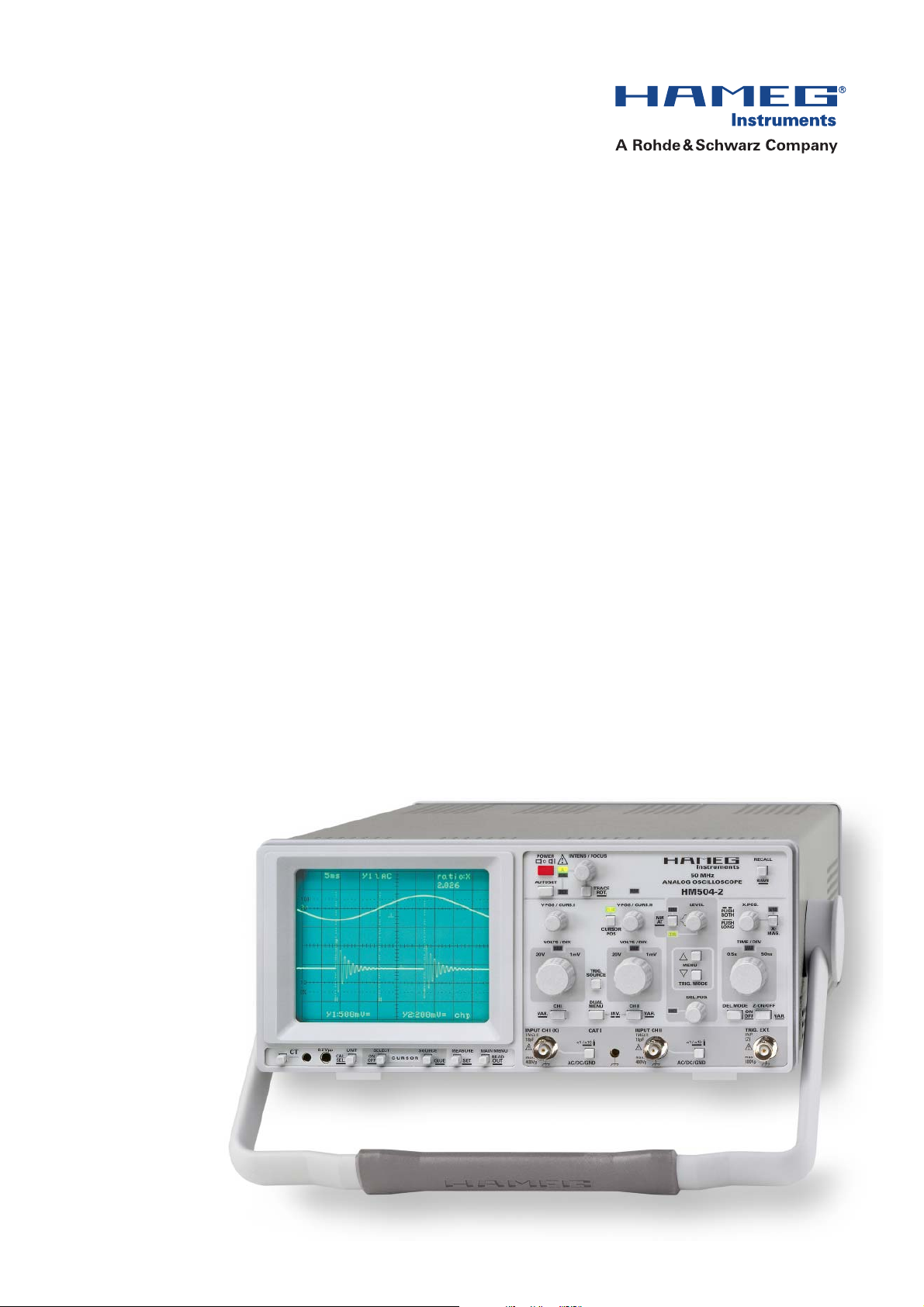
Oscilloscope

HM504-2

Manual

English

Page 2

Contents

CE-Declaration of Conformity ........................................... 4

General Information regarding the CE-marking .............. 4

Specifications ...................................................................... 5

General Information ........................................................... 6

Symbols............................................................................ 6

Use of tilt handle .............................................................. 6

Safety ............................................................................... 6

Intended purpose and operating conditions .................... 6

EMC ................................................................................. 7

Warranty ........................................................................... 7

Maintenance .................................................................... 7

Protective Switch-Off ....................................................... 7

Power supply .................................................................... 7

Type of signal voltage .................................................... 8

Amplitude Measurements ............................................... 8

Total value of input voltage .............................................. 9

Time Measurements........................................................ 9

Rise Time Measurement .................................................. 10

Connection of Test Signal................................................. 10

Controls and Readout ........................................................ 11

A: Menu Display and Operation....................................... 11

B: READOUT Information................................................. 12

C: Descriptions of Controls .............................................. 12

3 3

Oscilloscope

HM504-2

Menu .................................................................................... 23

First Time Operation ........................................................... 24

Trace Rotation TR ............................................................. 24

Probe compensation and use .......................................... 24

Adjustment at 1 kHz......................................................... 24

Adjustment at 1 MHz ....................................................... 24

Operating modes of the vertical

amplifiers in Yt mode. ........................................................ 25

X-Y Operation ................................................................... 25

Phase comparison with Lissajous figures ....................... 26

Phase difference measurement

in DUAL mode (Yt) ........................................................... 26

Phase difference measurement in DUAL mode .............. 26

Measurement of an amplitude modulation ..................... 26

Triggering and time base ................................................... 27

Automatic Peak (value) -Triggering................................... 27

Normal Triggering ............................................................. 28

SLOPE ....................................................................... 28

Trigger coupling ................................................................ 28

Triggering of video signals ............................................... 28

Line / Mains triggering (~)................................................ 29

Alternate triggering .......................................................... 29

External triggering ............................................................ 29

Trigger indicator ”TR” ...................................................... 30

HOLD OFF-time adjustment ............................................ 30

Delay / After Delay Triggering ........................................... 30

AUTO SET ............................................................................ 32

Mean Value Display ............................................................ 32

Component Tester ............................................................... 33

General ............................................................................. 33

Using the Component Tester ........................................... 33

Test Procedure ................................................................. 33

Test Pattern Displays ........................................................ 33

Testing Resistors .............................................................. 33

Testing Capacitors and Inductors..................................... 33

Testing Semiconductors .................................................. 34

Testing Diodes.................................................................. 34

Testing Transistors ............................................................ 34

In-Circuit Tests .................................................................. 34

Adjustments ........................................................................ 35

RS-232 Interface - Remote Control ................................... 35

Safety ............................................................................... 35

Operation ......................................................................... 35

RS-232 Cable.................................................................... 35

RS-232 protocol................................................................ 35

Baud-Rate Setting ............................................................ 35

Data Communication ....................................................... 35

Front Panel HM504-2 .......................................................... 36

Subject to change without notice

Page 3

General information regarding the CE marking

Herstellers HAMEG Instruments GmbH Manufacturer Industriestraße 6 Fabricant D-63533 Mainhausen

Die HAMEG Instruments GmbH bescheinigt die Konformität für das Produkt The HAMEG Instruments GmbH herewith declares conformity of the product HAMEG Instruments GmbH déclare la conformite du produit

Bezeichnung / Product name / Designation:

Oszilloskop/Oscilloscope/Oscilloscope

Typ / Type / Type: HM504-2

mit / with / avec: –

Optionen / Options / Options: –

mit den folgenden Bestimmungen / with applicable regulations / avec les directives suivantes

EMV Richtlinie 89/336/EWG ergänzt durch 91/263/EWG, 92/31/EWG EMC Directive 89/336/EEC amended by 91/263/EWG, 92/31/EEC Directive EMC 89/336/CEE amendée par 91/263/EWG, 92/31/CEE

Niederspannungsrichtlinie 73/23/EWG ergänzt durch 93/68/EWG Low-Voltage Equipment Directive 73/23/EEC amended by 93/68/EEC Directive des equipements basse tension 73/23/CEE amendée par 93/68/CEE

KONFORMITÄTSERKLÄRUNG DECLARATION OF CONFORMITY DECLARATION DE CONFORMITE

Angewendete harmonisierte Normen / Harmonized standards applied / Normes harmonisées utilisées

Sicherheit / Safety / Sécurité EN 61010-1: 2001 / IEC (CEI) 1010-1: 2001

Messkategorie / Measuring category / Catégorie de mesure: I Verschmutzungsgrad / Degree of pollution / Degré de pollution: 2

Elektromagnetische Verträglichkeit / Electromagnetic compatibility / Compatibilité électromagnétique

EN 61326-1/A1 :1997 + A1:1998 + A2 :2001/IEC 61326 :1997 + A1 :1998 + A2 :2001 Störaussendung / Radiation / Emission: Tabelle / table / tableau 4; Klasse / Class /Classe Störfestigkeit / Immunity / Imunitee: Tabelle / table / tableau A1.

EN 61000-3-2/A14 Oberschwingungsströme / Harmonic current emissions / Émissions de courant harmonique: Klasse / Class / Classe D.

EN 61000-3-3 Spannungsschwankungen u. Flicker / Voltage ﬂ uctuations and ﬂ icker / Fluctuations de tension et du ﬂ icker.

Datum / Date / Date Unterschrift / Signature / Signatur

25.6.2003

G. Hübenett Product Manager

General information regarding the CE marking

HAMEG instruments fulﬁ ll the regulations of the EMC directive. The conformity test made by HAMEG is based on the actual generic- and product standards. In cases where different limit values are applicable, HAMEG applies the severer standard. For emission the limits for residential, commercial and light industry are applied. Regarding the immunity (susceptibility) the limits for industrial environment have been used. The measuring- and data lines of the instrument have much inﬂ uence on emmission and immunity and therefore on meeting the acceptance limits. For different applications the lines and/or cables used may be different. For measurement operation the following hints and conditions regarding emission and immunity should be observed:

1. Data cables

For the connection between instruments resp. their interfaces and external devices, (computer, printer etc.) sufﬁ ciently screened cables must be used. Without a special instruction in the manual for a reduced cable length, the maximum cable length of a dataline must be less than 3 meters and not be used outside buildings. If an interface has several connectors only one connector must have a connection to a cable. Basically interconnections must have a double screening. For IEEEbus purposes the double screened cables HZ72S and HZ72L from HAMEG are suitable.

cable HZ72 from HAMEG is suitable.

2. Signal cables

Basically test leads for signal interconnection between test point and instrument should be as short as possible. Without instruction in the manual for a shorter length, signal lines must be less than 3 meters and not be used outside buildings. Signal lines must screened (coaxial cable - RG58/U). A proper ground connection is required. In combination with signal generators double screened cables (RG223/U, RG214/U) must be used.

3. Inﬂ uence on measuring instruments

Under the presence of strong high frequency electric or magnetic ﬁ elds, even with careful setup of the measuring equipment an inﬂ uence of such signals is unavoidable. This will not cause damage or put the instrument out of operation. Small deviations of the measuring value (reading) exceeding the instruments speciﬁ cations may result from such conditions in individual cases.

4. RF immunity of oscilloscopes

4.1 Electromagnetic RF ﬁ eld The inﬂ uence of electric and magnetic RF ﬁ elds may become visible (e.g. RF superimposed), if the ﬁ eld intensity is high. In most cases the coupling into the oscilloscope takes place via the device under test, mains/line supply, test leads, control cables and/or radiation. The device under test as well as the oscilloscope may be effected by such ﬁ elds. Although the interior of the oscilloscope is screened by the cabinet, direct radiation can occur via the CRT gap. As the bandwidth of each ampliﬁ er stage is higher than the total –3dB bandwidth of the oscilloscope, the inﬂ uence RF ﬁ elds of even higher frequencies may be noticeable.

4.2 Electrical fast transients / electrostatic discharge Electrical fast transient signals (burst) may be coupled into the oscilloscope directly via the mains/line supply, or indirectly via test leads and /or control cables. Due to the high trigger and input sensitivity of the oscilloscopes, such normally high signals may effect the trigger unit and/or may become visible on the CRT, which is unavoidable. These effects can also be caused by direct or indirect electrostatic discharge.

HAMEG Instruments GmbH

Subject to change without notice

Page 4

Subject to change without notice

HM504-2

� 2 Channels with deflection coefficients 1mV/div.…20V/div.

� Time Base 50ns /div.…0.5s/div.,

with X Magnification to 10ns/div.

� Low Noise Measuring Amplifiers with high pulse fidelity

� Triggering 0…100MHz from 5mm signal level

� Time Base delay provide high X Magnification

of any portion of the signal

� 100MHz 4-Digit Frequency Counter,

Cursor and Automatic Measurement

� Save/Recall Memories for Instrument Settings

� Readout, Autoset, no Fan

� Yt, XY and component-test modes

� RS-232 Interface (for parameter queries and control only)

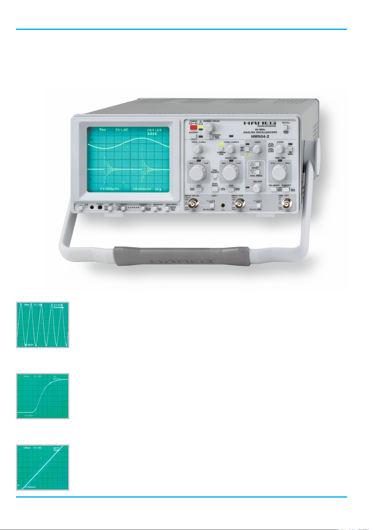
5 0 M H z An a lo g O s c i ll o s co p e

H M 5 04 - 2

HM504-2

Optimum deflection linearity

Rise-time measurement with cursor

Full screen display of 50 MHz sine wave

Page 5

50MHz Analog Oscilloscope HM504-2

All data valid at 23 °C after 30 minute warm-up

Vertical Deflection

Operating Modes: Channel 1 or 2 only

Channels 1 and 2 (alternate or chopped) Sum or Difference of CH 1 and CH 2

Invert: CH 2 XY Mode: CH 1 (X) and CH 2 (Y) Bandwidth: 2 x 0…50 MHz (-3 dB) Rise Time: ‹ 7 ns Deflection Coefficient: 1-2-5 Sequence

1…2 mV/div.: ±

5 % (0…10 MHz (-3 dB)) 5 mV/div.…20V/div.: ± 3 % (0…50MHz (-3 dB)) Variable (uncalibrated): ›2.5:1 to ›50 V/div.

Input Impedance: 1 MΩ II 15 pF Input Coupling: DC, AC, GND (ground) Max. Input Voltage: 400 V (DC + peak AC)

Triggering

Automatic (Peak to Peak): 20 Hz…100MHz (≥ 5 mm) Normal with Level Control: 0…100 MHz (≥ 5 mm) Slope: Rising or falling Sources: Channel 1 or 2, CH 1/CH 2 alternate

(≥ 8 mm), Line and External

Coupling: AC (10 Hz…100MHz), DC (0…100 MHz),

HF (50 kHz…100MHz), LF (0…1.5 kHz)

Trigger Indicator: LED Triggering after Delay: with Level Control and Slope selection External Trigger Signal: ≥ 0.3 V

(0…50 MHz)

Active TV sync. separator: Field and Line, +/-

Horizontal Deflection

Time Base: 50 ns/div.…0.5 s/div. (1-2-5 Sequence)

Accuracy: ± 3 % Variable (uncalibrated): › 2.5 :1 to › 1.25 s/div.

X Magnification x 10: up to 10 ns/div. (± 5 %)

Accuracy: ± 5 %

Delay (selectable): 200

ns…140 ms (variable)

Hold-Off Time: variable to approx. 10 : 1 XY Bandwidth X amplifier: 0…3 MHz (-3dB) XY Phase shift ‹ 3 °: ‹120 kHz

Operation/Readout/Control

Manual: via controls Autoset: automatic signal related parameter settings Save and Recall: 9 instrument parameter settings Readout: display of menu, parameters, cursors and

results

Autom. Measurement: Freq./Period, V

, Vpp, Vp+, Vp-,

Trigger Level

Cursor Measurement: Δt, 1/Δt, tr, ΔV, V to GND, Gain, Ratio X and Y Frequency counter: 4 digit (0.01 % ± 1 digit) 0.5 Hz…100MHz Interface: RS-232

Component Tester

Test Voltage: approx. 7V

rms

(open circuit)

Test Current: max. 7 mA

rms

(short-circuit)

Test Frequency: approx. 50Hz Test Connection: 2 banana jacks 4 mm Ø

One test circuit lead is grounded via protective earth (PE)

Miscellaneous

CRT: D14-363GY, 8 x 10 div. with internal graticule Acceleration Voltage: approx. 2kV Trace Rotation: adjustable on front panel Z-input (Intens. modulation): max. + 5 V (TTL) Calibrator Signal (Square Wave):0.2V, 1 Hz…1MHz (tr ‹ 4 ns), DC Power Supply (Mains): 105…253 V, 50/60 Hz ± 10 %, CAT II Power Consumption: approx. 34Watt at 230 V/50 Hz Safety class: Safety class I (EN61010-1) Operating temperature: +5…+40°C Storage temperature: -20…+70°C Rel. humidity: 5…80% (non condensing) Dimensions (W x H x D): 285 x 125 x 380 mm Weight: approx. 5.4kg

Device control and Parameter query, no CRT content transfer possible.

Accessories supplied: Line Cord, Operators Manual and Software for Windows on CD-ROM, 2 Probes 1:1 /10:1 (HZ154), RS-232 Interface

Optional accessories:

HZ14 Interface cable (serial) 1:1 HZ20 Adapter, BNC to 4mm banana HZ33 Test cable 50Ω, BNC/BNC, 0,5m HZ34 Test cable 50Ω, BNC/BNC, 1m HZ43 19''-Rackmount Kit 3RU HZ51 Probe 10:1 (150MHz) HZ52 Probe 10:1 RF (250MHz) HZ53 Probe 100:1 (100MHz) HZ56-2 AC/DC Current probe HZ70 Opto Interface (with optical fiber cable) HZ100 Differential probe 20:1 / 200:1 HZ109 Differential probe 1:1 / 10:1 HZ115 Differential probe 100:1 / 1000:1 HZ200 Probe 10:1 with auto attenuation ID (250MHz) HZ350 Probe 10:1 with automatically identification (350MHz) HZ355 Slimline probe 10:1 with automatically identification (500MHz) HZO20 High voltage probe 1000:1 (400MHz,1000Vrms) HZO30 Active probe 1GHz (0,9pF, 1MΩ, including many accessories) HZO50 AC/DC Current probe 20A, DC...100kHz HZO51 AC/DC Current probe 1000A, DC...20kHz

HM504-2E/091109/ce · Subject to changes · © HAMEG Instruments GmbH®· DQS-certified in accordance with DIN EN ISO 9001:2000, Reg.-No.: DE-071040 QM

HAMEG Instruments GmbH · Industriestr. 6 · D-63533 Mainhausen · Tel +49 (0) 6182 800 0 · Fax +49 (0) 6182 800100 · www.hameg.com · info@hameg.com

w w w . h a m e g . c o m

50MHz Analog Oscilloscope HM504-2

All data valid at 23 °C after 30 minute warm-up

Vertical Deflection

Operating Modes: Channel 1 or 2 only

Channels 1 and 2 (alternate or chopped) Sum or Difference of CH 1 and CH 2

Invert: CH 2 XY Mode: CH 1 (X) and CH 2 (Y) Bandwidth: 2 x 0…50 MHz (-3 dB) Rise Time: ‹ 7 ns Deflection Coefficient: 1-2-5 Sequence

1…2 mV/div.: ±

5 % (0…10 MHz (-3 dB)) 5 mV/div.…20V/div.: ± 3 % (0…50MHz (-3 dB)) Variable (uncalibrated): › 2.5:1 to › 50V/div.

Input Impedance: 1 MΩ II 15 pF Input Coupling: DC, AC, GND (ground) Max. Input Voltage: 400 V (DC + peak AC)

Triggering

Automatic (Peak to Peak): 20 Hz…100MHz (≥ 5 mm) Normal with Level Control: 0…100 MHz (≥ 5 mm) Slope: Rising or falling Sources: Channel 1 or 2, CH 1/CH 2 alternate

(≥ 8 mm), Line and External

Coupling: AC (10 Hz…100MHz), DC (0…100 MHz),

HF (50 kHz…100MHz), LF (0…1.5 kHz)

Trigger Indicator: LED Triggering after Delay: with Level Control and Slope selection External Trigger Signal: ≥ 0.3 V

(0…50 MHz)

Active TV sync. separator: Field and Line, +/-

Horizontal Deflection

Time Base: 50 ns/div.…0.5 s/div. (1-2-5 Sequence)

Accuracy: ± 3 % Variable (uncalibrated): › 2.5 :1 to › 1.25 s/div.

X Magnification x 10: up to 10 ns/div. (± 5 %)

Accuracy: ± 5 %

Delay (selectable): 200

ns…140 ms (variable)

Hold-Off Time: variable to approx. 10 : 1 XY Bandwidth X amplifier: 0…3 MHz (-3dB) XY Phase shift ‹ 3 °: ‹120 kHz

Operation/Readout/Control

Manual: via controls Autoset: automatic signal related parameter settings Save and Recall: 9 instrument parameter settings Readout: display of menu, parameters, cursors and

results

Autom. Measurement: Freq./Period, V

, Vpp, Vp+, Vp-,

Trigger Level

Cursor Measurement: Δt, 1/Δt, tr, ΔV, V to GND, Gain, Ratio X and Y Frequency counter: 4 digit (0.01 % ± 1 digit) 0.5 Hz…100MHz Interface: RS-232

Component Tester

Test Voltage: approx. 7V

rms

(open circuit)

Test Current: max. 7 mA

rms

(short-circuit)

Test Frequency: approx. 50Hz Test Connection: 2 banana jacks 4 mm Ø

One test circuit lead is grounded via protective earth (PE)

Miscellaneous

Device control and Parameter query, no CRT content transfer possible.

Accessories supplied: Line Cord, Operators Manual and Software for Windows on CD-ROM, 2 Probes 1:1 /10:1 (HZ154), RS-232 Interface

Optional accessories:

Speciﬁcations

Subject to change without notice

Page 6

General information

Please check the instrument for mechanical damage or loose parts immediately after unpacking. In case of damage we advise to contact the sender. Do not operate.

List of symbols used

Consult the manual High voltage

Important note Ground

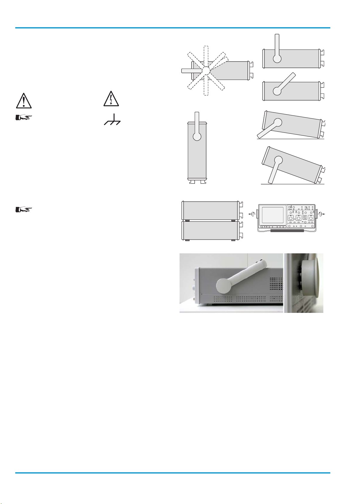
Positioning the instrument

As can be seen from the ﬁ gures, the handle can be set into different positions: A and B = carrying C = horizontal operating D and E = operating at different angles F = handle removal T = shipping (handle unlocked)

Attention!

When changing the handle position, the instru-

ment must be placed so that it can not fall (e.g. placed on a table). Then the handle locking knobs must be simultaneously pulled outwards and rotated to the required position. Without pulling the locking knobs they will latch in into the next locking position.

PUOPFGkT

PUOPFGkT PUOPFGkT

PUOPFGkT

PUOGkT

PUOPFGkT

HM507

PUOPFGkT

PUOPFGkT PUOPFGkT PUOPFGkT PUOPFGkT

PUOPFGkT

PUOPFGkT PUOPFGkT

PUk PUk PUk PUk PUk PUk

PUkT

HGOPFFD

PUOPFGkT

PUkT

INPUT CHI OPK HJ

PUkT

VBN

PUOPFGkT

HJKL

PUOPFGkT

PUkT

PUOPFGkT

HGOFFD

PUkT

INPUT CHI

HAMEG

OPK

VBN

PUOPFGkT

HJKL

Handle mounting/dismounting

The handle can be removed by pulling it out further, depending on the instrument model in position B or F.

Safety

The instrument fulﬁ ls the VDE 0411 part 1 regulations for electrical measuring, control and laboratory instruments and was manufactured and tested accordingly. It left the factory in perfect safe condition. Hence it also corresponds to European Standard EN 61010-1 resp. International Standard IEC 1010-1. In order to maintain this condition and to ensure safe operation the user is required to observe the warnings and other directions for use in this manual. Housing, chassis as well as all measuring terminals are connected to safety ground of the mains. All accessible metal parts were tested against the mains with 200 V

The oscilloscope may only be operated from mains outlets with a safety ground connector. The plug has to be installed prior to connecting any signals. It is prohibited to separate the safety ground connection.

Most electron tubes generate X-rays; the ion dose rate of this instrument remains well below the 36 pA /kg permitted by law.

In case safe operation may not be guaranteed do not use the instrument any more and lock it away in a secure place.

. The instrument conforms to safety class I.

Safe operation may be endangered if any of the following was noticed:

– in case of visible damage. – in case loose parts were noticed – if it does not function any more. – after prolonged storage under unfavourable conditions (e.g.

like in the open or in moist atmosphere).

– after any improper transport (e.g. insufﬁ cient packing not

conforming to the minimum standards of post, rail or transport company)

Proper operation

Please note: This instrument is only destined for use by personnel well instructed and familiar with the dangers of electrical measurements.

For safety reasons the oscilloscope may only be operated from mains outlets with safety ground connector. It is prohibited to separate the safety ground connection. The plug must be inserted prior to connecting any signals.

Subject to change without notice

Page 7

General information

CAT I

This oscilloscope is destined for measurements in circuits not connected to the mains or only indirectly. Direct measurements, i.e. with a galvanic connection to circuits corresponding to the categories II, III, or IV are prohibited!

The measuring circuits are considered not connected to the mains if a suitable isolation transformer fulﬁ lling safety class II is used. Measurements on the mains are also possible if suitable probes like current probes are used which fulﬁ l the safety class II. The measurement category of such probes must be checked and observed.

Measurement categories

The measurement categories were derived corresponding to the distance from the power station and the transients to be expected hence. Transients are short, very fast voltage or current excursions which may be periodic or not.

Measurement CAT IV: Measurements close to the power station, e.g. on electricity meters

Measurement CAT III: M e a su r e me n t s in t h e in t e r io r o f b u il d i n gs ( p o w e r d i s t ri b u t i on i n s ta l lations, mains outlets, motors which are permanently installed).

Measurement CAT II: Measurements in circuits directly connected to the mains (household appliances, power tools etc).

Measurement CAT I: Electronic instruments and circuits which contain circuit breakers resp. fuses.

Warranty and repair

HAMEG instruments are subjected to a strict quality control. Prior to leaving the factory, each instrument is burnt-in for 10 hours. By intermittent operation during this period almost all defects are detected. Following the burn-in, each instrument is tested for function and quality, the speciﬁ cations are checked in all operating modes; the test gear is calibrated to national standards.

The warranty standards applicable are those of the country in which the instrument was sold. Reclamations should be directed to the dealer.

Only valid in EU countries

In order to speed reclamations customers in EU countries may also contact HAMEG directly. Also, after the warranty expired, the HAMEG service will be at your disposal for any repairs.

Return material authorization (RMA):

Prior to returning an instrument to HAMEG ask for a RMA number either by internet (http://www.hameg.com) or fax. If you do not have an original shipping carton, you may obtain one by calling the HAMEG service dept (++49 (0) 6182 800 500) or by sending an email to service@hameg.com.

Maintenance

Clean the outer shell using a dust brush in regular intervals. Dirt can be removed from housing, handle, all metal and plastic parts using a cloth moistened with water and 1 % detergent. Greasy dirt may be removed with benzene (petroleum ether) or alcohol, there after wipe the surfaces with a dry cloth. Plastic parts should be treated with an antistatic solution destined for such parts. No ﬂ uid may enter the instrument. Do not use other cleansing agents as they may adversely affect the plastic or lacquered surfaces.

Environment of use.

The oscilloscope is destined for operation in industrial, business, manufacturing, and living sites.

Environmental conditions

Operating ambient temperature: +5 °C to +40 °C. During transport or storage the temperature may be –20 °C to +70°C.

Please note that after exposure to such temperatures or in case of condensation proper time must be allowed until the instrument has reached the permissible temperature, resp. until the condensation has evaporated before it may be turned on! Ordinarily this will be the case after 2 hours. The oscilloscope is destined for use in clean and dry environments. Do not operate in dusty or chemically aggressive atmosphere or if there is danger of explosion.

The operating position may be any, however, sufﬁ cient ventilation must be ensured (convecti on cooling). P rolonged operation requires the horizontal or inclined position.

Do not obstruct the ventilation holes!

Speciﬁ cations are valid after a 30 minute warm-up period between 15 and 30 degr. C. Speciﬁ cations without tolerances are average values.

Line voltage

The instrument has a wide range power supply from 105 to 253 V, 50 or 60 Hz ±10%. There is hence no line voltage selector.

The line fuse is accessible on the rear panel and part of the line input connector. Prior to exchanging a fuse the line cord must be pulled out. Exchange is only allowed if the fuse holder is undamaged, it can be taken out using a screwdriver put into the slot. The fuse can be pushed out of its holder and exchanged.

The holder with the new fuse can then be pushed back in place against the spring. It is prohibited to ”repair“ blown fuses or to bridge the fuse. Any damages incurred by such measures will void the warranty.

Type of fuse:

Size 5 x 20 mm; 250V~, C; IEC 127, Bl. III; DIN 41 662 (or DIN 41 571, Bl. 3). Cut off: slow blow (T) 0,8A.

Subject to change without notice

Page 8

Type of signal voltage

The oscilloscope HM504-2 allows examination of DC voltages and most repetitive signals in the frequency range up to at least 50 MHz (–3 dB). The Y amplifiers have been designed for minimum overshoot and therefore permit a true signal display.

The display of sinusoidal signals within the bandwidth limits causes no problems, but an increasing error in measurement due to gain reduction must be taken into account when measuring high frequency signals. This error becomes noticeable at approx. 14 MHz. At approx. 30 MHz the reduction is approx. 10% and the real voltage value is 11% higher. The gain reduction error can not be defined exactly as the –3 dB bandwidth of the Y amplifiers differs between 50 MHz and 55 MHz.

When examining square or pulse type waveforms, attention must be paid to the harmonic content of such signals. The repetition frequency (fundamental frequency) of the signal must therefore be significantly smaller than the upper limit frequency of the Y amplifiers.

Displaying composite signals can be difficult, especially if they contain no repetitive higher amplitude content that can be used for triggering. This is the case with bursts, for instance. To obtain a well triggered display in this case, the assistance of the variable holdoff function or the delayed time base may be required. Television video signals are relatively easy to trigger using the built in TV Sync Separator (TV).

For optional operation as a DC or AC voltage amplifier, each Y amplifier input is provided with a DC/AC switch. DC coupling should only be used with a series connected attenuator probe or at very low frequencies, or if the measurement of the DC voltage content of the signal is absolutely necessary.

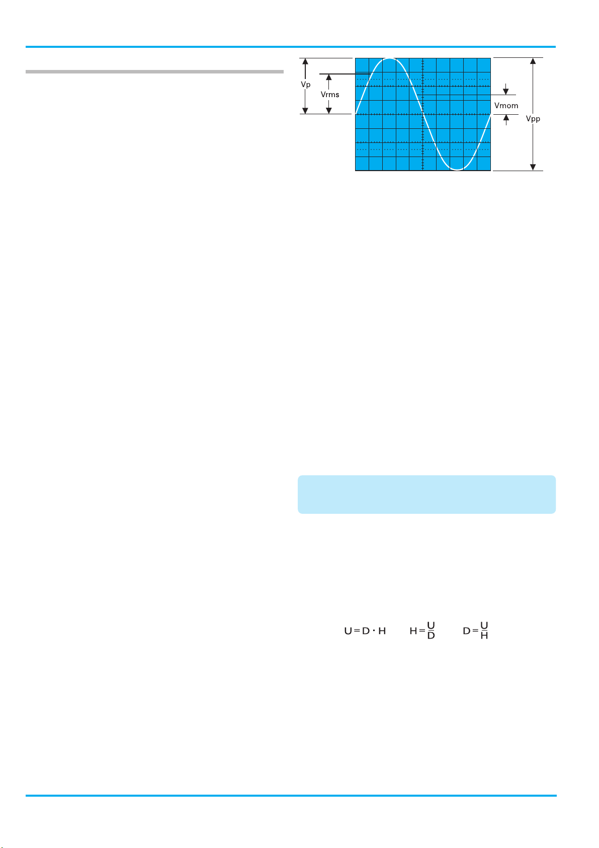
Voltage values of a sine curve

= effective value; Vp = simple peak or crest value;

rms

= peak to peak value; V

= momentary value.

mom

The minimum signal voltage which must be applied to the Y input for a trace of 1div height is 1mV

(± 5%) with this deflection

coefficient displayed on the screen (readout) and the vernier switched off (VAR-LED dark). However, smaller signals than this may also be displayed. The deflection coefficients are indicated in mV/div or V/div (peak to peak value).

The magnitude of the applied voltage is ascertained by multiplying the selected deflection coefficient by the vertical display height in div. If an attenuator probe x10 is used, a further multiplication by a factor of 10 is required to ascertain the correct voltage value. This factor can be entered into the oscilloscope’s memory for automatic calculation.

For exact amplitude measurements, the variable control (VAR) must be set to its calibrated detent CAL position.

With the variable control activated the deflection sensitivity can be reduced up to a ratio of 2.5 to 1 (

readout”

). Therefore any intermediate value is possible within

please note ”controls and

the 1-2-5 sequence of the attenuator(s).

When displaying very low frequency pulses, the flat tops may be sloping with AC coupling of the Y amplifier (AC limit frequency approx. 1.6 Hz for 3dB). In this case, DC operation is preferred, provided the signal voltage is not superimposed on too high a DC level. Otherwise a capacitor of adequate capacitance must be connected to the input of the Y amplifier with DC coupling. This capacitor must have a sufficiently high breakdown voltage rating. DC coupling is also recommended for the display of logic and pulse signals, especially if the pulse duty factor changes constantly. Otherwise the display will move upwards or downwards at each change. Pure direct voltages can only be measured with DC coupling.

Amplitude Measurements

In general electrical engineering, alternating voltage data normally refers to effective values (rms = root mean square value). However, for signal magnitudes and voltage designations in oscilloscope measurements, the peak to peak voltage (V

) value

is applied. The latter corresponds to the real potential difference between the most positive and most negative points of a signal waveform.

If a sinusoidal waveform, displayed on the oscilloscope screen, is to be converted into an effective (rms) value, the resulting peak to peak value must be divided by 2 x √2 = 2.83. Conversely, it should be observed that sinusoidal voltages indicated in Vrms

) have 2.83 times the potential difference in Vpp. The

eff

relationship between the different voltage magnitudes can be seen from the following figure.

With direct connection to the Y input, signals up to 400 V

may be displayed (attenuator set to 20 V/div, variable control to 2.5:1).

With the designations

H = display height in div, U = signal voltage in V

at the Y input,

D = deflection coefficient in V/div at attenuator switch,

the required value can be calculated from the two given quantities:

However, these three values are not freely selectable. They have to be within the following limits (trigger threshold, accuracy of reading):

H between 0.5 and 8div, if possible 3.2 to 8div, U between 0.5 mV

and 160 Vpp,

D between 1 mV/div and 20 V/div in 1-2-5 sequence.

Examples:

Set deflection coefficient D = 50 mV/div 0.05 V/div, observed display height H = 4.6 div, required voltage U = 0.05x4.6 = 0.23 V

Subject to change without notice

Page 9

Type of signal voltage

Input voltage U = 5 Vpp, set deflection coefficient D = 1 V/div, required display height H = 5:1 = 5 div.

Signal voltage U = 230 V

x 2√2 = 651 V

rms

(voltage > 160 Vpp, with probe 10:1: U = 65.1 Vpp), desired display height H = min. 3.2 div, max. 8 div,

max. deflection coefficient D = 65.1:3.2 = 20.3 V/div, min. deflection coefficient D = 65.1:8 = 8.1 V/div, adjusted deflection coefficient D = 10 V/div.

The previous examples are related to the CRT graticule reading. The results can also be determined with the aid of the DV cursor measurement (

please note ”controls and readout”

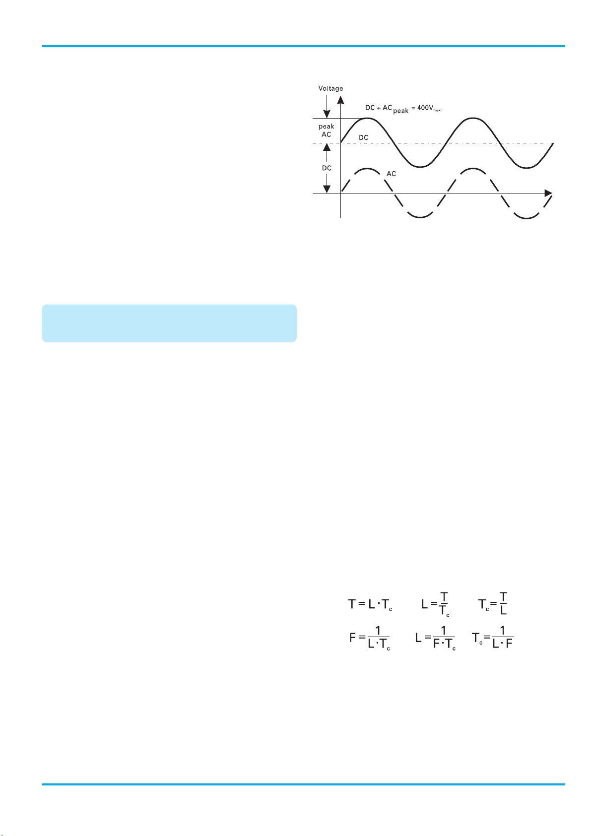
The input voltage must not exceed 400 V, irrespective of polarity.

If an AC voltage which is superimposed on a DC voltage is applied, the maximum peak value of both voltages must not exceed + or –400 V. So for AC voltages with a mean value of zero volt the maximum peak to peak value is 800 Vpp.

If attenuator probes with higher limits are used, the probes limits are valid only if the oscilloscope is set to DC input coupling.

If DC voltages are applied under AC input coupling conditions the oscilloscope maximum input voltage value remains 400 V.

The attenuator consists of a resistor in the probe and the 1 MOhm input resistor of the oscilloscope, which is disabled by the AC input coupling capacity when AC coupling is selected. This also applies to DC voltages with superimposed AC voltages.

It also must be noted that due to the capacitive reactance of the AC input coupling capacitor, the attenuation ratio depends on the signal frequency. For sine wave signals with frequencies higher than 40 Hz this influence is negligible.

Apart from the above listed exceptions, HAMEG 10:1 probes can be used for DC measurements up to 600 V or AC voltages (with a mean value of zero volt) of 1200 V allows for use up to 1200 V DC or 2400 V

. The 100 :1 probe HZ53

for AC.

It should be noted that its AC peak value is derated at higher frequencies. If a normal x10 probe is used to measure high voltages, there is the risk that the compensation trimmer bridging the attenuator series resistor will break down, causing damage to the input of the oscilloscope.

Total value of input voltage

The dotted line shows a voltage alternating at zero volt level. If superimposed on a DC voltage, the addition of the positive peak and the DC voltage results in the max. voltage (DC + ACpeak).

Time Measurements

As a rule, most signals to be displayed are periodically repeating processes, also called periods. The number of periods per second is the repetition frequency. Depending on the time base setting (TIME/DIV. knob) indicated by the readout, one or several signal periods or only a part of a period can be displayed. The time coefficients are stated in ms/div, µs/div or ns/div. The following examples are related to the CRT graticule reading. The results can also be determined with the aid of the Dt and 1/Dt cursor measurement (

please note ”controls and readout”

The duration of a signal period or a part of it is determined by multiplying the relevant time (horizontal distance in div) by the (calibrated) time coefficient displayed in the readout.

Uncalibrated, the time base speed can be reduced until a maximum factor of 2.5 is reached. Therefore any intermediate value is possible within the 1-2-5 sequence.

With the designations

L = displayed wave length in div of one period, T = time in seconds for one period, F = recurrence frequency in Hz of the signal, Tc = time coefficient in ms, µs or ns/div and the relation F = 1/T, the following can be stated:

However, if for example only the residual ripple of a high voltage is to be displayed on the oscilloscope, a normal x10 probe is sufficient. In this case, an appropriate high voltage capacitor (approx. 22 - 68nF) must be connected in series with the input tip of the probe.

With Y-POS. control (input coupling to GD) it is possible to use a horizontal graticule line as reference line for ground potential before the measurement. It can lie below or above the horizontal central line according to whether positive and/or negative deviations from the ground potential are to be measured.

Subject to change without notice

However, these four values are not freely selectable. They have to be within the following limits:

L between 0.2 and 10 div, if possible 4 to 10 div, T between 10 ns and 5 s, F between 0.5 Hz and 100 MHz, Tc between 100 ns/div and 500 ms/div in 1-2-5 sequence

(with X-MAG. (x10) inactive), and

Tc between 10 ns/div and 50 ms/div in 1-2-5 sequence (with

X-MAG. (x10) active).

Page 10

Type of signal voltage

Examples:

Displayed wavelength L = 7 div, set time coefficient Tc = 100 ns/div,

-9

thus period T = 7 x 100 x 10 thus freq. F = 1/(0.7 x 10

= 0.7 µs

-6

) = 1.428 MHz.

Signal period T = 1s, set time coefficient Tc = 0.2 s/div, thus wavelength L = 1/0.2 = 5 div.

Displayed ripple wavelength L = 1 div, set time coefficient Tc = 10 ms/div,

-3

thus ripple freq. F = 1/(1 x 10 x 10

) = 100 Hz.

TV Line frequency F = 15625 Hz, set time coefficient Tc = 10 µs/div, required wavelength L = 1/(15,625 x 10-5) = 6.4 div.

Sine wavelength L = min. 4 div, max. 10 div, Frequency F = 1 kHz, max. time coefficient Tc = 1/(4 x 10 min. time coefficient Tc = 1/(10 x 10

) = 0.25 ms/div,

) = 0.1 ms/div, set time coefficient Tc = 0.2 ms/div, required wavelength L = 1/(103 x 0.2 x 10-3) = 5 div.

Displayed wavelength L = 0.8 div, set time coefficient Tc = 0.5 µs/div, pressed X-MAG. (x10) button: Tc = 0.05 µs/div,

-6

thus freq. F = 1/(0.8 x 0.05 x 10 thus period T = 1/(25 x 10

) = 25 MHz,

) = 40 ns.

If the time is relatively short as compared with the complete signal period, an expanded time scale should always be applied (X-MAG. (x10) active). In this case, the time interval of interest can be shifted to the screen center using the X-POS. control.

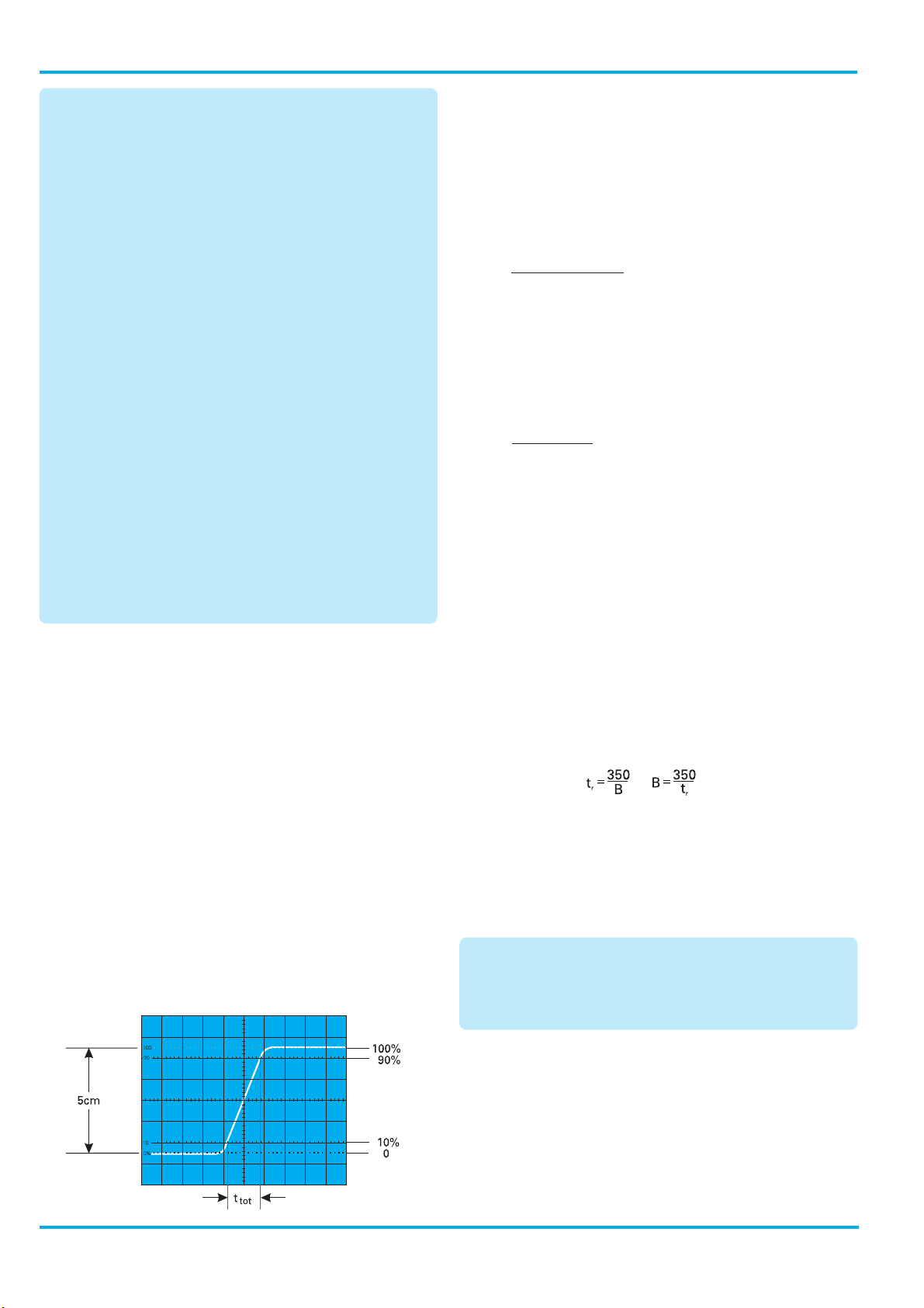
Rise Time Measurement

When investigating pulse or square waveforms, the critical feature is the rise time of the voltage step. To ensure that transients, ramp-offs, and bandwidth limits do not unduly influence the measuring accuracy, the rise time is generally measured between 10% and 90% of the vertical pulse height. For measurement, adjust the Y deflection coefficient using its variable function (uncalibrated) together with the Y-POS. control so that the pulse height is precisely aligned with the 0% and 100% lines of the internal graticule. The 10% and 90% points of the signal will now coincide with the 10% and 90% graticule lines. The risetime is given by the product of the horizontal distance in div between these two coincident points and the calibrated time coefficient setting. The fall time of a pulse can also be measured by using this method. The following figure shows correct positioning of the oscilloscope trace for accurate rise time measurement.

With a time coefficient of 10 ns/div (X x10 magnification active), the example shown in the above figure results in a total measured risetime of

= 1.6 div x 10 ns/div = 16 ns

tot

When very fast risetimes are being measured, the risetimes of the oscilloscope amplifier and of the attenuator probe have to be deducted from the measured time value. The risetime of the signal can be calculated using the following formula.

= √ t

In this t

– t

tot

osc

is the total measured risetime, t

tot

oscilloscope amplifier (approx. 7 ns), and t probe (e.g. = 2 ns). If t

– t

is the risetime of the

osc

is greater than 100 ns, then t

tot

the risetime of the

can be

tot

taken as the risetime of the pulse, and calculation is unnecessary.

Calculation of the example in the figure above results in a signal risetime:

= √162 – 72 – 22 = 14.25 ns

The measurement of the rise or fall time is not limited to the trace dimensions shown in the above diagram. It is only particularly simple in this way. In principle it is possible to measure in any display position and at any signal amplitude. It is only important that the full height of the signal edge of interest is visible in its full length at not too great steepness and that the horizontal distance at 10% and 90% of the amplitude is measured. If the edge shows rounding or overshooting, the 100% should not be related to the peak values but to the mean pulse heights. Breaks or peaks (glitches) next to the edge are also not taken into account. With very severe transient distortions, the rise and fall time measurement has little meaning. For amplifiers with approximately constant group delay (therefore good pulse transmission performance) the following numerical relationship between rise time tr (in ns) and bandwidth B (in MHz) applies:

Connection of Test Signal

In most cases, briefly depressing the AUTOSET causes a useful signal related instrument setting. The following explanations refer to special applications and/or signals, demanding a manual instrument setting.

in the section ”controls and readout”.

Caution: When connecting unknown signals to the oscilloscope input, always use automatic triggering and set the input coupling switch to AC. The attenuator should initially be set to 20 V/div.

The description of the controls is explained

Sometimes the trace will disappear after an input signal has been applied. Then a higher deflection coefficient (lower input sensitivity) must be chosen until the vertical signal height is only 3 – 8 div. With a signal amplitude greater than 160 V

and the deflection

coefficient (VOLTS/DIV.) in calibrated condition, an attenuator probe must be inserted before the Y input. If, after applying the signal, the trace is nearly blanked, the period of the signal is probably substantially longer than the set time deflection coefficient (TIME/DIV.). It should be switched to an adequately larger time coefficient.

Subject to change without notice

Page 11

Controls and Readout

The signal to be displayed can be connected directly to the Y input of the oscilloscope with a shielded test cable such as HZ32 or HZ34, or reduced through a x10 or x100 attenuator probe. The use of test cables with high impedance circuits is only recommended for relatively low frequencies (up to approx. 50 kHz). For higher frequencies, the signal source must be of low impedance, i.e. matched to the characteristic resistance of the cable (as a rule 50 Ohm). Especially when transmitting square and pulse signals, a resistor equal to the characteristic impedance of the cable must also be connected across the cable directly at the Y-input of the oscilloscope. When using a 50 Ohm cable such as the HZ34, a 50 Ohm through termination type HZ22 is available from HAMEG. When transmitting square signals with short rise times, transient phenomena on the edges and top of the signal may become visible if the correct termination is not used. A terminating resistance is sometimes recommended with sine signals as well. Certain amplifiers, generators or their attenuators maintain the nominal output voltage independent of frequency only if their connection cable is terminated with the prescribed resistance. Here it must be noted that the terminating resistor HZ22 will only dissipate a maximum of 2 Watts. This power is reached with 10 V attenuator probe is used, no termination is necessary. In this case, the connecting cable is matched directly to the high impedance input of the oscilloscope. When using attenuator probes, even high internal impedance sources are only slightly loaded (approx. 10 MOhm II 12 pF or 100 MOhm II 5 pF with HZ53). Therefore, if the voltage loss due to the attenuation of the probe can be compensated by a higher amplitude setting, the probe should always be used. The series impedance of the probe provides a certain amount of protection for the input of the Y amplifier. Because of their separate manufacture, all attenuator probes are only partially compensated, therefore accurate compensation must be performed on the oscilloscope

compensation )

Standard attenuator probes on the oscilloscope normally reduce its bandwidth and increase the rise time. In all cases where the oscilloscope bandwidth must be fully utilized (e.g. for pulses with steep edges) we strongly advise using the probes HZ51 (x10) HZ52 (x10 HF) and HZ54 (x1 and x10). This can save the purchase of an oscilloscope with larger bandwidth. The probes mentioned have an HF-adjustment in addition to low frequency calibration adjustment. Thus a group delay correction to the upper limit frequency of the oscilloscope is possible with the aid of a 1 MHz calibrator, e.g. HZ60.

In fact the bandwidth and rise time of the oscilloscope are not noticeably changed with these probe types and the waveform reproduction fidelity can even be improved because the probe can be matched to the oscilloscope’s individual pulse response.

If a x10 or x100 attenuator probe is used, DC input coupling must always be used at voltages above 400 V. With AC coupling of low frequency signals, the attenuation is no longer independent of frequency, pulse tops can show pulse tilts. Direct voltages are suppressed but charge the oscilloscope input coupling capacitor concerned. Its voltage rating is max. 400 V (DC + peak AC). DC input coupling is therefore of quite special importance with a x100 attenuation probe which usually has a voltage rating of max. 1200 V (DC + peak AC). A capacitor of corresponding capacitance and voltage rating may be connected in series with the attenuator probe input for blocking DC voltage (e.g. for hum voltage measurement).

(28.3 Vpp) with sine signal. If a x10 or x100

rms

(see Probe

With all attenuator probes, the maximum AC input voltage must be derated with frequency, usually above 20 kHz. Therefore the derating curve of the attenuator probe type concerned must be taken into account. The selection of the ground point on the test object is important when displaying small signal voltages. It should always be as close as possible to the measuring point. If this is not done, serious signal distortion may result from spurious currents through the ground leads or chassis parts. The ground leads on attenuator probes are also particularly critical. They should be as short and thick as possible. When the attenuator probe is connected to a BNC-socket, a BNC adapter should be used. In this way ground and matching problems are eliminated. Hum or interference appearing in the measuring circuit (especially when a small deflection coefficient is used) is possibly caused by multiple grounding because equalizing currents can flow in the shielding of the test cables (voltage drop between the protective conductor connections, caused by external equipment connected to the mains/line, e.g. signal generators with interference protection capacitors).

Controls and Readout

A: Basic settings

The following description assumes that:

1. “Component Tester” is switched off.

2. The following settings are present under MAIN MENU > SETUP & INFO > MISCELLANEOUS:

2.1 CONTROL BEEP and ERROR BEEP activated (x),

2.2 QUICK START not activated.

3. The screen Readout is visible.

The LED indicators on the large front panel facilitate operation and provide additional information. Electrical end positions of controls are indicated by acoustic signal (beep).

All controls, except the power switch (POWER), are electronically set and interrogated. Thus, all electronically set functions and their current settings can be stored and also remotely controlled.

B: Menu Display and Operation

Operation of some pushbuttons activates the display of menus. There are Standard and Pulldown Menus.

Standard menus:

When a standard menu is displayed, all other readout information (e.g. parameter settings) are switched off. The readout then consists of the menu headline, and the respective menu functions. At the bottom of the graticule are displayed symbols and commands which can be operated by the pushbuttons related to them below.

“Esc” CT pushbutton [37] switches one step back in the menu hierarchy.

“Exit” SELECT – ON/OFF pushbutton [34] closes the menu and switches back to the operating conditions present before calling the menu.

The pushbuttons underneath the triangle symbols pointing upwards UNIT CAL.SEL. [35] and downwards SOURCE GLUE [33] enable you to select one item which becomes highlighted.

Subject to change without notice

Page 12

Controls and Readout

“SET” MAIN MENU-pushbutton [31] calls the selected menu

item, starts a function or switches a function on/off.

Pulldown menus:

After pressing a pushbutton which calls a Pulldown menu, the instrument parameter settings are still displayed. The readout only changes in respect to the called parameter (e.g. input coupling) and now shows all selectable parameter options (in case of input coupling: AC, DC and GND). The previously displayed parameter doesn‘t change but is displayed highlighted. Each time the pushbutton is briefly pressed the next parameter becomes active and highlighted, as long as the Pulldown menu is displayed. Without further pressing the pushbutton, the Pulldown menu extinguishes after a few seconds and the selected parameter is displayed in the normal way.

C: READOUT Information

The readout alphanumerically displays the scope parameter settings, measurement results and CURSOR lines. Which information is displayed depends on the actual instrument settings. The following list contains the most important display information.

Top of the graticule from left to right: 1st time deflection coefficient 2nd trigger source, slope and coupling 3rd operating condition of delay time base 4th measuring results

Bottom of the graticule from left to right: 1st probe symbol (x10), Y deflection coefficient and input

coupling channel I 2nd “+” symbol (addition) 3rd probe symbol (x10), Y deflection coefficient and input

coupling channel II 4th channel mode

The trigger point symbol is displayed at the left graticule border line. The CURSOR lines can take any position within the graticule.

[2] AUTOSET

Briefly pressing this pushbutton results in an automatic instrument setting selecting Yt mode as the default. The instrument is set to the last used Yt mode setting (CH I, CH II or DUAL). The instrument is set automatically to normal (undelayed) time base mode, even if the previous Yt mode was present in combination with search (“sea”), delay (“del”) or triggered delay (“dTr”) time base mode.

Please also note ”AUTO-

SET” in section “First Time Operation”.

Automatic CURSOR positioning:

If CURSOR lines are displayed and AUTOSET is chosen the CURSOR lines are set automatically under suitable conditions and the readout briefly displays “SETTING CURSOR”.

If the signal height is insufficient, the CURSOR lines do not change. In DUAL mode the CURSOR lines are related to the signal which is used for internal triggering.

Voltage CURSOR

If voltage measurement is present, the CURSOR lines are automatically set to the positive and negative peak value of the signal. The accuracy of this function decreases with higher frequencies and is also influenced by the signal‘s pulse duty factor.

Time/Frequency CURSOR

If complex waveforms such as video signals are applied, the cursor lines may not align exactly with one period and give a false reading.

[3] INTENS/FOCUS – Knob with associated LEDs and TRACE

ROT.-pushbutton. If the readout (RO) is not switched off, briefly pressing the READOUT pushbutton switches over the INTENS/FOCUS knob function indicated by a LED in the sequence A, FOC, RO, A. In condition READOUT deactivated, the switching sequence is A, FOC, A.

Description of Controls

The large front panel is, as usual with Hameg oscilloscopes, marked with several fields.

The following controls and LED indicators are located on the top, to the right of the screen, above the horizontal line.

1 3 4 5

POWER

AUTOSET

[1] POWER – Pushbutton and symbols for ON (I) and OFF (O).

INTENS / FOCUS

TRACE

ROT.

Instruments

50 MHz

ANALOG OSCILLOSCOPE

HM504-2

RECALL

SAVE

After the oscilloscope is switched on, all LEDs are lit and an automated instrument test is performed. During this time the HAMEG logo and the software version are displayed on the screen. After the internal test is completed successfully, the overlay is switched off and the normal operation mode is present. Then the last used settings become activated and LED [3] indicates the ON condition.

“A”:

The INTENS/FOCUS control knob adjusts the signal(s) intensity. Turning this knob clockwise increases the intensity. Only the minimum required trace intensity should be used, depending on signal parameters, oscilloscope settings and light conditions.

“FOC”:

The INTENS/FOCUS control knob adjusts both the trace and the readout sharpness. Note: The electron beam diameter gets larger with a higher trace intensity and the trace sharpness decreases. This can be corrected to a certain extent. Assuming that the trace sharpness was set to optimum in the screen centre, it is unavoidable that the trace sharpness decreases with an increasing distance from the centre. Since the settings of the signal(s) intensity (A) and the READOUT (RO) are usually different, the FOCUS should be set for optimum signal(s) sharpness. The sharpness of the READOUT then can be improved by reducing the READOUT intensity.

“RO”:

The INTENS/FOCUS control knob adjusts the READOUT intensity. Turning this knob clockwise increases and counter clockwise decreases the intensity. Only the minimum required intensity should be used.

Subject to change without notice

Page 13

Controls and Readout

TRACE ROT. (trace rotation) is selected by pressing and

holding the pushbutton. This causes the display “Trace Rot. with Int.” (trace rotation by use of INTENS/FOCUS knob) and allows you to compensate the influence of the Earth’s magnetic field on the trace deflection. To avoid misadjustment due to unavoidable deflection non linearities, set the trace to the graticule centre (Y-POS/CURS.I and X-POS. control). After the trace has been set parallel to the horizontal graticule line using INTENS/FOCUS, press “SAVE” to store the last setting. Further information can be found in section “First Time Operation” under “Trace Rotation”.

1 3 4 5

POWER

AUTOSET

INTENS / FOCUS

TRACE

ROT.

Instruments

50 MHz

ANALOG OSCILLOSCOPE

HM504-2

RECALL

SAVE

[4] RM

The remote control mode can be switched on or off (”RM” LED dark) via the RS-232 interface. When the ”RM” LED is lit, all electronically selectable controls on the front panel are inactive. This state can be cancelled by depressing the AUTO SET pushbutton provided it was not deactivated via the interface.

[5] SAVE / RECALL – Pushbutton for instrument settings

The instrument contains 9 non volatile memories. These can be used by the operator to save instrument settings and to recall them.

SAVE:

Press and hold the RECALL/SAVE button to start a storage process. This causes the SAVE menu (Standard menu, note “B: Menu-Display and Operation”) to be displayed. Choose the memory location cipher (highlighted) by pressing a pushbutton underneath the triangle symbols. Briefly press the pushbutton underneath “SET” to store the last instrument setting and return from menu display to previous mode. If the SAVE function was called inadvertently, it can be switched off with “Esc”. Switching the instrument off automatically stores the current settings in memory location 9 (PWR OFF = Power Off), with the effect that different settings previously stored in this location get lost. To prevent this, RECALL 9 before switching the instrument off.

RECALL:

Briefly pressing calls the RECALL menu. You can select the required memory location using a “triangle” pushbutton. Recall the previously stored instrument settings by briefly pressing the “SET” pushbutton or briefly press “Esc” if the function was called inadvertently.

Attention: When an instrument setting is recalled, the current signal may not be optimally displayed unless similar (frequency, amplitude) to that used when the setting was stored.

The setting controls and LED’s for the Y amplifiers, modes, triggering and time base are located underneath the sector of the front panel described above.

Y-POS / CURS.I

VOLTS / DIV.

20V 1mV 20V 1mV 0.5s 50ns

CH I CH II DEL.MODE Z-ON/OFF

VAR .

7 98 11 131210

Y-POS / CURS.II LEVEL X-POS.

TRIG.

SOURCE

DUAL

CURSOR

POS

VOLTS / DI V.

INV.

TRIG. MODE

DEL.POS.

VAR .

PUSH BOTH

PUSH LONG

TIME / DIV.

OFF

x10

X-

MAG.

VAR .

[6] Y-POS/CURS. I – Control knob with two functions.

This knob allows position control of channel I trace or CURSOR line(s). Briefly pressing the CURSOR POS pushbutton [7] selects the function. If the CURSOR line(s) are not displayed the CURS. I function is not selectable.

Y-POS:

The vertical trace position of channel I can be set with this control knob, if the CURSOR POS LED isn’t lit. In addition (“add”) mode both Y-POS/CURS. I [6] and Y-POS/CURS. II [8] control knobs are active. If the instrument is set to XY mode this control knob is inactive and the X-POS. [12] knob must be used for horizontal positioning.

DC voltage measurement:

If no signal is applied at the INPUT CH I [25], the vertical trace position represents 0 Volt. This is the case if INPUT CH I [25] or in addition (ADD) mode, both INPUT CH I [25] and INPUT CH II [28], are set to GND (ground) [26; 29] and automatic triggering AT [9] is present to make the trace visible. The trace can then be set to the vertical position best suited for the following DC voltage measurement. After switching GND (ground) off and selecting DC input coupling, a DC signal applied at the input changes the trace position in vertical direction. The DC voltage then can be determined by taking the deflection coefficient, the probe factor and the trace position change with respect to the previous 0 Volt position into account.

”0-Volt”-Symbol:

The READOUT indicates the “0-Volt” trace position of channel

⊥⊥

I by a ”

⊥” symbol to the left of the screen‘s vertical centre line

⊥⊥

in CHI and DUAL mode. When Y position is used, this symbol changes to an “arrow” symbol pointing outside the graticule just before the trace goes outside the graticule limits. If addition mode (“add”) is present just one ”⊥” symbol is visible. In XY mode the “0-Volt” trace position for channel I (X) and channel II (Y) is symbolised by “triangle” symbols at the right graticule border (Y) and above the Y deflection coefficient display. The “triangle” symbol(s) point(s) outside the graticule when the “0-Volt” trace position is outside the graticule.

CURS.I:

The CURSOR lines marked by the symbol “I” can be shifted by the Y-POS/CURS. I control knob, if the CURSOR POS LED [7] lit.

Subject to change without notice

Page 14

Controls and Readout

[7] CURSOR POS – Pushbutton and LED.

Briefly pressing this pushbutton determines the function of the Y-POS/CURS.I [6] and Y-POS/CURS.II [8] controls. If the LED is not lit the Y position control function is active. Provided that the CURSOR lines are activated, the LED can be switched on by briefly pressing the CURSOR POSpushbutton. Then the controls [6] and [8] are switched over from Y position to CURSOR position control CURS.I [6] and CURS.II [8]. Briefly pressing this pushbutton once again switches back to the Y position control function.

Y-POS / CURS.I

VOLTS / DIV.

20V 1mV 20V 1mV 0.5s 50ns

CH I CH II DEL.MODE Z-ON/OFF

VAR .

7 98 11 131210

Y-POS / CURS.II LEVEL X-POS.

TRIG.

SOURCE

DUAL

CURSOR

POS

VOLTS / DIV.

INV.

TRIG. MODE

DEL.POS.

VAR .

PUSH BOTH

PUSH LONG

TIME / DIV.

OFF

[8] Y-POS/CURS. II – Control knob with two functions.

This knob enables position control of channel II trace or CURSOR line(s). Briefly pressing the CURSOR POSpushbutton [7] selects the function. If the CURSOR line(s) are not displayed the CURS. I function is not selectable.

Y-POS:

The vertical trace position of channel II can be set with this control knob, if the CURSOR POS LED isn’t lit. In addition (“add”) mode both, Y-POS/CURS. I [6] and Y-POS/CURS. II [8] control knobs are active. If the instrument is set to XY mode, this control knob is inactive and the X-POS.-knob [12] must be used for horizontal positioning.

x10

X-

MAG.

If addition mode (“add”) is present just one ”^” symbol is visible. In XY mode the “0 Volt” trace position for channel I (X) and channel II (Y) is symbolised by “triangle” symbols at the right graticule border (Y) and above the Y deflection coefficient display. The “triangle” symbol (s) point (s) outside the graticule when the “0-Volt” trace position is outside the graticule.

CURS. II:

The CURSOR lines marked by the symbol “II” can be shifted by the Y-POS/CURS. II control knob, if the CURSOR POS LED [7] lit.

[9] NM AT – Pushbutton with a double function and asso-

ciated NM LED.

NM / AT selection:

Press and hold the pushbutton to switch over from automatic (peak value) to normal triggering (NM LED above the pushbutton lit) and vice versa. If the LED is dark, automatic or automatic peak value triggering is selected.

VAR .

AT:

Automatic triggering can be carried out with or without peak capture. In both cases the LEVEL control [11] is effective and

the trace is visible even if no signal is applied or trigger settings are unsuitable. Signal frequencies below the automatic trigger frequency can not be triggered as the automatic trigger cycle starts to early for such signals.

In the automatic peak value triggering condition the LEVEL control [11] range is limited to the trigger signal positive and negative peak values. Automatic triggering without peak value detection enables the trigger point to be set outside the signal amplitude range. In the latter case, although untriggered, there is still a signal display.

Whether the peak value detection is active or not depends on the operating mode and the selected trigger coupling. The actual state is recognised by the behaviour of the trigger point symbol when changing the LEVEL setting.

DC voltage measurement:

If no signal is applied at the INPUT CH II [28], the vertical trace position represents 0 Volt. This is the case if INPUT CH

II [28] or in addition (ADD) mode, both, INPUT CH I [25] and INPUT CH II [28], are set to GND (ground) [26; 29] and

automatic triggering AT [9] is present to make the trace visible.

The trace can then be set to the vertical position best suited for the following DC voltage measurement. After switching GND (ground) off and selecting DC input coupling, a DC signal applied at the input changes the trace position in vertical direction. The DC voltage then can be determined by taking the deflection coefficient,

the probe factor and the trace position change with respect to the previous 0 Volt position into account.

”0-Volt”-Symbol:

The READOUT indicates the “0-Volt” trace position of channel II by a ”^” symbol to the right of the screen‘s vertical centre line in CH II and DUAL mode. When Y-position is used, this symbol changes to an “arrow” symbol pointing outside the graticule just before the trace goes outside the graticule limits.

NM:

Normal triggering disables both the automatic trigger and the peak value detection so even low frequency signals can be displayed in a stable manner. Without suitable input signal height, trigger coupling and LEVEL settings, no trace will be displayed. The last LEVEL setting of the time base is stored, then the control again becomes active when selecting triggering after delay DEL.MODE (“dTr”) time base mode (quasi 2 base). In combination with In “dTr” mode the LEVEL control is operative for the “2nd time base”.

/ \ (Slope selection): Each time this pushbutton is briefly pressed, the slope direction switches from falling edge to rising edge and vice versa. The current setting is displayed in the readout by a slope symbol. The last setting in undelayed time base mode is stored and still active if triggered delay (“dTr”) time base mode is selected. This allows for a different slope setting for the triggered DELAY (DTR) time base mode.

[10] TR – Trigger indicator LED.

The TR LED is lit in Yt mode if the triggering conditions are met for the first trigger unit used in undelayed time base

Subject to change without notice

time

Page 15

Controls and Readout

mode. Whether the LED flashes or is lit constantly depends on the frequency of the trigger signal.

[11] LEVEL – Control knob.

Turning the LEVEL knob causes a different trigger point setting (voltage). The trigger unit starts the time base when the edge of a trigger signal crosses the trigger point. In most Yt modes the trigger point is displayed in the readout by the symbol on the left vertical graticule line. If the trigger point symbol would overwrite other readout information or would be invisible when being set above or below the screen, the symbol changes and an arrow indicates in which vertical direction the trigger point has left the screen. The trigger point symbol is automatically switched off in those modes where there is no direct relation between the trigger signal and the displayed signal. The last setting in undelayed time base mode is stored and still active if triggered delay (“dTr”) time base mode is selected. This allows for a different level setting for the triggered delay (“dTr”) time base mode.

[12] X-POS. – Control knob.

This control knob enables an X position shift of the signal(s) in Yt and XY mode. In combination with X magnification x10 (Yt mode) this function makes it possible to shift any part of the signal on the screen.

[13] X-MAG. x10 – Pushbutton and LED.

Each time this pushbutton is pressed the x10 LED located above is switched on or off. If the x10 LED is lit, the signal display is expanded 10 fold in all time deflection settings > 50ns/div. At 50 ns/div only the expansion is 5 fold and yields 10ns/div. As the X expansion results in a higher time base speed (lower time deflection coefficient), all time and frequency relevant information in the readout is switched over. After activating X MAG. x10, the visible part of the signal is that which was previously at the graticule centre. The interesting part of the signal can be made visible with aid of the X-POS. [12] control.

This pushbutton is not operative in XY mode.

[15] CH I VAR. – Pushbutton with two functions.

Pressing and holding this pushbutton selects the VOLTS/ DIV. [14] control knob function between attenuator and

vernier (variable). The current setting is displayed by the

VAR-LED located above the knob.

CH I mode:

Briefly pressing the CHI button sets the instrument to channel I (Mono CH I) mode. The deflection coefficient displayed in the readout indicates the current conditions (”Y1...”). If neither external nor line (mains) triggering was active, the internal trigger source automatically switches over to channel I and the READOUT displays “Y1, trigger slope, trigger coupling”. The last function setting of the VOLTS/DIV [14] knob remains unchanged. All channel I related controls are active if the input [25] is not set to GND [26].

VAR.:

After switching the VAR-LED [14] on, the deflection coefficient is still calibrated. Turning the VOLTS/DIV. [14] control knob counter clockwise reduces the signal height and the deflection coefficient becomes uncalibrated. The readout then displays e.g. ”Y1>...” indicating the uncalibrated condition instead of ”Y1:...”. Pressing and holding the CHI pushbutton again switches the LED off, sets the deflection coefficient into calibrated condition and activates the attenuator function. The previous vernier setting will not be stored.

[16] DUAL MENU – Pushbutton with multiple functions.

Switchover on DUAL (two channel), ADDITION and XY operation: Briefly pressing selects DUAL mode if channel I (mono) or channel II (mono) mode had been present before. Then the deflection coefficients of both channels and the channel switchover mode (alt or chp) become visible on the READOUT. The last trigger conditions (source, slope and coupling) remain unchanged, but can be changed. Pressing and holding the DUAL pushbutton switches directly to XY mode if channel I (mono) or channel II (mono) mode had been present before. On condition XY mode pressing the pushbutton switches back to DUAL mode.

[14] VOLTS/DIV. – Control knob for channel I with a double

function. This control is active only if channel I is enabled and it‘s input coupling (AC or DC) is activated. Channel I is active in CH I (Mono), DUAL, Addition (“add”) and XY mode. The knob is automatically disabled if the channel related to it is switched off, or if the input coupling is set to GND (ground). Y-deflection coefficient setting (input attenuator): This function is available if the VAR. LED is dark. Turning the control knob clockwise increases the sensitivity (decreases the deflection coefficient) in a 1-2-5 sequence and decreases the sensitivity (increases the deflection coefficient) if turned in the opposite direction (ccw.). The available range is from 1mV/div up to 20V/div. The deflection coefficients and additional information regarding the active channel(s) are displayed in the readout, e.g. ”Y1: deflection coefficient, input coupling”. The ”:” symbolizes calibrated measuring conditions and is replaced by the ”>” symbol in uncalibrated conditions.

VAR.: The vernier (variable) function is described under item VAR [15].

Subject to change without notice

Choosing the channel switch over or sub menu: Once DUAL mode is active, briefly pressing the (Dual) pushbutton opens a Pulldown menu with the current mode displayed highlighted. The menu offers “chp” (chopped DUAL), “alt” (alternate DUAL), “add” (Addition) and “XY” mode.

As long as the Pulldown menu is displayed, briefly pressing the pushbutton selects the next mode and highlights the actual setting. Please note “B: Menu Display and Operation“. If “add” (Addition) mode is activated, briefly pressing the pushbutton switches over to DUAL mode, without displaying the Pulldown menu. All channel related controls are effective as long as the input coupling is not set to GND [26, 29].

DUAL mode:

On the right of the channel II (Y2:...) deflection coefficient the READOUT displays the channel switch over mode. “alt” indicates alternate and „chp“, chopped switch over. The channel switch over is automatically selected by the time

Page 16

Controls and Readout

base setting, but can be changed in the pulldown menu. The oscilloscope automatically determines the channel switching mode after a change of the time base setting.

“chp” (Chopped):

Indicates chopped mode, whereby the channel switching occurs constantly between channel I and II during each sweep. This channel switching mode occurs when any time base setting between 500 ms/div and 500 µs/div has been chosen.

“alt” (Alternate):

Indicates alternate channel switching. After each time base sweep the instrument internally switches over from channel I to channel II and vice versa. This channel switching mode is automatically selected if any time coefficient from 200 µs/ div to 50 ns/div is active.

“add” (Addition):

The readout indicates this mode by a ”+” sign located between both channel deflection coefficients. In addition mode, two signals (channel I and II) are displayed as one signal. The Y position of the signal can be influenced by both Y-POS/CURS.I [6] and Y-POS/CURS.II [8] controls. For correct measurements the deflection coefficients for both channels must be equal. While the trigger mode is not affected, the trigger point symbol is switched off. Whether the algebraic sum (addition) or the difference (subtraction) of both input signals is displayed, depends on the phase relationship and the INV (invert function) setting.

XY mode: In XY mode the deflection coefficients are displayed as ”X...” for channel I and ”Y...” for channel II, followed by ”XY”. The following READOUT information is switched off:

time deflection coefficient, trigger source, slope, coupling and trigger point symbol. In addition to all trigger and time base related controls, the Y- POS/CURS.I-knob [7] is deactivated. For X-position alteration, the X-POS.-knob [12] can be used.

The front panel shows that the DUAL MENU push button [16] can also be depressed together with the CH II pushbutton [19]. Please note item [19].

the signal used for triggering originates. The measuring amplifiers (internal triggering) or the BNC socket which serves as an input for externally applied signals (external triggering) can be used as a trigger source.

Single channel operation (CH I or CH II):

Briefly pressing switches the trigger source over without displaying the Pulldown menu. During single channel operation the internal trigger signal (originating from channel I or channel II) or the external trigger signal can be chosen.

DUAL and Addition mode:

Briefly pressing opens the trigger source Pulldown menu with the actual setting highlighted. Please note “B: Menu

Display and Operation”.

The following listing shows the possible trigger sources and how they are indicated by the READOUT. Their availability depends on the actual channel operation mode.

„Y1“: The measurement amplifier of channel I serves as Pulldown trigger source.

„Y2“: The measurement amplifier of channel II serves as trigger source.

„alt“: Alternate triggering can be chosen if DUAL mode is present. In alternate trigger mode, the switch over of the internal trigger sources “Y1” and “Y2” is carried out synchronously with the alternate channel switching and the trigger point symbol is switched off.

As alternate triggering requires alternate channel operation, alternate channel switching is set automatically. A change of the time coefficient then has no affect regarding the channel switching mode. The following trigger coupling settings can not be chosen in combination with alternate triggering: TVL, TVF and line (mains).

If “add” (addition) or delayed time base mode (“sea”, “del” or “dTr”) is present, alternate triggering is not available. Therefore alternate triggering is automatically switched off if one of these modes has been chosen.

Y-POS / CURS.I

VOLTS / DIV.

20V 1mV 20V 1mV 0.5s 50ns

CH I CH II DEL.MODE Z-ON/OFF

VAR .

TRIG.

SOURCE

DUAL MENU

CURSOR

POS

[17] TRIG. SOURCE – Pushbutton.

This pushbutton is for trigger source selection and deactivated if line (mains) triggering is selected or XY operation is chosen. The term “trigger source” describes the source from which

7 98 11 131210

Y-POS / CURS.II LEVEL X-POS.

VOLTS / DIV.

TRIG. MODE

INV.

VAR .

DEL.POS.

PUSH BOTH

PUSH LONG

OFF

TIME / DIV.

x10

X-

MAG.

“ext”: External trigger mode is available in all time base and trigger coupling modes except line/mains triggering. Then the TRIG.EXT. BNC-socket [30] serves as the external trigger signal input. On external triggering mode, the intensity modulation (Z), which might have been present before, is automatically switched off.

[18] VOLTS/DIV. – Control knob for channel II with a double

function. This control is active only if channel II is enabled and it‘s input coupling (AC or DC) is activated. Channel II is active in CH II (Mono), DUAL, Addition (“add”) and XY mode. The knob is

VAR .

automatically disabled if the channel related to it is switched off, or if the input coupling is set to GND (ground).

Y-deflection coefficient setting (input attenuator):

This function is available if the VAR. LED is dark.

Turning the control knob clockwise increases the sensitivity (decreases the deflection coefficient) in a 1-2-5-sequence and decreases the sensitivity (increases the deflection

Subject to change without notice

Page 17

Controls and Readout

coefficient) if turned in the opposite direction (ccw.). The available range is from 1mV/div up to 20V/div.

The deflection coefficients and additional information regarding the active channel(s) are displayed in the readout, e.g. ”Y2: deflection coefficient, input coupling”. The ”:” symbolizes calibrated measuring conditions and is replaced by the ”>” symbol in uncalibrated conditions.

VAR.: The vernier (variable) function is described under item VAR [19].

[19] CH II - VAR. – Pushbutton with several functions.

Pressing and holding this pushbutton selects the VOLTS/ DIV. [18] control knob function between attenuator and vernier (variable). The current setting is displayed by the

VAR-LED located above the knob.

CH II mode:

Briefly pressing the CH II-button sets the instrument to channel II (Mono CH II) mode. The deflection coefficient displayed in the readout indicates the current conditions (”Y2...”). If neither external nor line (mains) triggering was active, the internal trigger source automatically switches over to channel II and the READOUT displays “Y2, trigger slope, trigger coupling”. The last function setting of the VOLTS/DIV-knob [18] remains unchanged. All channel II related controls are active if the input [28] is not set to GND [29].

VAR.:

After switching the VAR-LED [18] on, the deflection coefficient is still calibrated. Turning the VOLTS/DIV.-control knob [18] counter clockwise reduces the signal height and the deflection coefficient becomes uncalibrated.

Y-POS / CURS.I

VOLTS / DIV.

20V 1mV 20V 1mV 0.5s 50ns

CH I CH II DEL.MODE Z-ON/OFF

VAR .

7 98 11 131210

Y-POS / CURS.II LEVEL X-POS.

TRIG.

SOURCE

DUAL MENU

CURSOR

POS

VOLTS / DI V.

INV.

TRIG. MODE

DEL.POS.

VAR .

PUSH

BOTH

PUSH LONG

TIME / DIV.

OFF

x10

X-

MAG.

VAR .

TVL: TV signal, line pulse triggering,

trigger point symbol switched off,

TVF: TV signal, frame pulse triggering,

trigger point symbol switched off.

~: line/mains triggering,

trigger point symbol switched off.

Line/mains triggering inactivates the TRIG. SOURCE-pushbutton [17].

In some trigger modes such as alternate triggering, some trigger coupling modes are automatically disabled and can not be selected.

[21] DEL.POS. HO LED – Control knob with double function and

related HO LED. The DEL.POS. -knob has two functions which depend on the actual time base mode.

The readout then displays e.g. ”Y2>...” indicating the uncalibrated condition instead of ”Y2:...”. Pressing and holding the CHI pushbutton again switches the LED off, sets the deflection coefficient into calibrated condition and activates the attenuator function. The previous vernier setting will not be stored.

INV.:

Briefly and simultaneously pressing the CHII and the DUALMENU (16) pushbutton switches the channel II invert function on or off. The invert ”on” condition is indicated by the readout with a horizontal bar above ”Y2” (Yt mode). The invert function causes the signal display of channel II to be inverted by 180°.

[20] TRIG. MODE – Pushbuttons.

Pressing one of these pushbuttons opens the trigger coupling Pulldown menu with the actual setting highlighted. Briefly pressing a pushbutton selects the trigger coupling. Please note “B: Menu Display and Operation”.

The term “trigger coupling” describes the way the trigger signal is connected to the trigger unit.

AC: DC content suppressed, DC: peak value detection inactive, HF: high pass filter cuts off frequencies below

approx. 50 kHz, trigger point symbol switched off

LF: low pass filter cuts off frequencies above

approx. 1.5 kHz,

1. DEL.POS. (delay position).

In the delay time base modes “sea” (search), “del”(delay) and “dTr” (triggered after delay) a delay time between the trigger event and the start of the trace can be set with the DEL.POS. control.

See DEL.MODE [23].

2. HO (holdoff time).

The holdoff time function can be activated if normal (undelayed) time base mode is present. On condition that the HO LED is not lit the holdoff time is set to minimum. The HO LED lights up and the holdoff time increases as the knob is rotated clockwise. A signal sounds on reaching the maximum holdoff time. Similarly in the opposite direction until minimum holdoff time is reached (HO LED extinguishes).

The holdoff time is automatically set to minimum when the time base is changed. (For the application of holdoff time setting see the paragraph with the same heading).

[22] TIME/DIV. – Control knob with a double function.

This control can be used for time coefficient selection in 1-25-sequence under calibrated condition when the VAR LED is not lit or as a vernier (variable) control (VAR LED lit).

Time coefficient setting:

In undelayed, delayed (“del”) and as delayed triggered (“dTr”) time base mode, this control serves as a time deflection coefficient selector. Rotating anticlockwise increases the deflection coefficient and rotating clockwise decreases the coefficient. The setting is displayed at the top left in the

Subject to change without notice

Page 18

Controls and Readout

Readout (e.g. “10 µs”). Depending on the time base mode the following ranges are available without taking X x10 into account.

Undelayed: 500 ms/div – 50 ns/div.

The following (principle) values depend on the time base setting in undelayed mode, as the undelayed time base always has to have the higher coefficient.

Search (“sea”): 20 ms/div – 100 ns/div.

Delay (“del”): 20 ms/div. – 50 ns/div.

Triggered after delay (“dTr): 20 ms/div – 50 ns/div.

VAR.:

The vernier (variable) function is described under item Z ON/ OFF VAR [24].

Y-POS / CURS.I

VOLTS / DIV.

20V 1mV 20V 1mV 0.5s 50ns

CH I CH II DEL.MODE Z-ON/OFF

VAR .

7 98 11 131210

Y-POS / CURS.II LEVEL X-POS.

TRIG.

SOURCE

DUAL MENU

CURSOR

POS

VOLTS / DIV.

INV.

TRIG. MODE

DEL.POS.

VAR .

PUSH BOTH

PUSH LONG

TIME / DIV.

OFF

x10

X-

MAG.

VAR .

Functions

“sea”:

In SEARCH mode, the holdoff time is automatically set to minimum and for the first few divisions the trace is blanked. The point at which the trace is unblanked can be varied with the DEL.POS [21] control (fine adjustment) from about 2 to 7 divisions. The blanked section serves as a guide to the delay time. The delay time is based on the current time deflection coefficient setting and can also be coarsely set with the TIME/DIV control (range: 20 ms to 100 ns). The signal position at which the unblanking occurs marks the trace start position which is present after switching over from “sea” to “del”. This enables lower time deflection coefficient settings for signal expansion.

“del”:

In DELAY mode, a trigger event does not start the trace at once but only initiates the delay time. After the delay time has elapsed the trace is started. Selecting lower time deflection coefficients (higher time base speed) cause a signal expansion in X direction. The DEL.POS [21] control can still be used for correcting the signal start position affected by the TIME/DIV setting.

Note: With higher expansion rates the trace intensity may reduce drastically.

“dTr”:

In triggered DELAY mode the first trigger unit, used for triggering in undelayed time base mode, starts the delay time as in “del” mode. After the delay time has elapsed the delay time base must be triggered by the second trigger unit, to

start and unblank the trace. The latter requires suited instrument settings (LEVEL, SLOPE) to enable triggering.

[23] DEL.MODE ON/OFF – Pushbutton with two functions.

ON/OFF function:

Pressing and holding this pushbutton switches over between delayed and undelayed time base mode. The actual setting is indicated by the READOUT. The delayed time base operation enables a magnified display in X direction which is otherwise only possible with a second time base.

a) Undelayed time base mode.

If on the right of the trigger READOUT information (source, slope, coupling) neither “sea”, “del” nor “dTr” is indicated, undelayed time base mode is present. Note: When the intensity modulation function is switched on, the letter “Z” is visible in this position on the screen.

b) Delayed time base mode.

Is indicated by the READOUT showing “sea”, “del” or “dTr”. If intensity modulation was chosen before switching over to delay time base mode, this function is automatically switched off and consequently the letter “Z” deleted.

Switching over from undelayed to delayed time base mode automatically selects “sea” (search) mode. Briefly pressing the pushbutton then opens a Pulldown menu for operating mode selection. Please note “B: Menu Display and Operation”. The following description assumes that in undelayed time base mode the trace starts at left edge of the graticule, with x10 X MAG. switched off.

Note: The trigger indicator LED (TR) [10] only indicates the trigger condition of the first trigger unit. It may be lit although the trigger conditions for the second time base are not met and the trace remains blanked.

As in “del” mode the DEL.POS [21] control can still be used. In contrast to complex signals the effect of this function may not be noticed with simple repetitive signals as the trigger point ‘hops’ from cycle to cycle, each being the same.

[24] Z ON/OFF VAR. – Pushbutton with two functions.

Z ON/OFF:

Briefly pressing the pushbutton switches over the function of the TRIG.EXT. BNC-socket [30] from external trigger input to intensity modulation input and vice versa. In connection with external triggering, delay time base (“sea”, “del” or “dTr”) and “Component Tester” mode, Z modulation can not be enabled.

Z modulation is shown on the READOUT to the right of “trigger source, slope and coupling” indicated by the letter “Z”. High TTL level (positive logic) gives blanking, dark, low level gives unblanking, bright. No higher voltages than +5 Volt are permitted.

VAR.:

Pressing and holding the button changes the function of the TIME/DIV. -knob [22] from time deflection coefficient switch to time vernier (fine adjustment) control and vice versa.

Subject to change without notice

Page 19

Controls and Readout

The current function is indicated by the VAR LED. The TIME/ DIV. knob functions as a vernier when the VAR LED is

switched on, but the time base setting remains calibrated until the (vernier) knob is operated. The readout now indicates e.g. ”>10ms” instead of ”10ms”. Rotating further anticlockwise increases the time deflection coefficient (uncalibrated) until the maximum is reached indicated by a beep. Rotating the knob clockwise has the opposite effect. Now, the vernier is again in the calibrated position and the symbol ”>” extinguishes.

Underneath the front panel sector described above, the BNC sockets and two pushbuttons are located.

INPUT CHI (X)

1MΩ II 18pF

! ! !

max. 400Vp

x1 / x10

AC/DC/GND

26 27

CAT

INPUT CHI (X)

1MΩ II 18pF

max. 400Vp

28 29 30

x1 / x10

AC/DC/GND

TRIG. EXT.

INP. (Z)

max. 100Vp

[25] INPUT CH I (X) – BNC socket.

This BNC socket is the signal input for channel I. The outer (ground) connection is galvanically connected to the instrument ground and consequently to the safety earth contact of the line/mains plug. The AC/DC/GND pushbutton [26] is assigned to the input. In XY mode, signals at this input are used for the X deflection.

[26] AC/DC/GND x1/x10 – Pushbutton with several functions.

AC/DC/GND:

Briefly pressing this pushbutton opens the input coupling Pulldown menu if a channel mode is present in which channel I is activated. The following input couplings are available: AC, DC and GND (ground). Please note “B: Menu Display and Operation”.

After the Pulldown menu has extinguished, the READOUT displays the present input coupling at the bottom right hand of ”Y1: deflection coefficient”; the “~“ symbol indicates AC, the “=” symbol DC and “GND” is for ground. The GND setting disables the input signal and the VOLTS/ DIV [14] knob. Then in automatic trigger mode (Yt) the undeflected trace is visible representing the 0 Volt trace position; in XY mode the X deflection is deactivated.

x1/x10:

Probe factor selection is performed by pressing and holding the pushbutton. This selects the indicated deflection coefficient of channel I displayed in the readout, between 1:1 and 10:1. In condition 10:1, the probe factor is thus indicated by a probe symbol displayed by the readout in front the channel information (e.g. ”probe symbol”, Y1...). In the case of cursor voltage measurement, the probe factor is automatically included.

Please note: The symbol should not be activated unless a x10 (10:1) attenuator probe is used.

[27] Ground socket 4mm banana socket galvanically connected

to safety earth. This socket can be used as reference potential connection for DC and low frequency signal measurement purposes and in “Component Tester” mode.

[28] INPUT CH II – BNC socket.

This BNC socket is the signal input for channel II. The outer (ground) connection is galvanically connected to the instrument ground and consequently to the safety earth contact of the line/mains plug. The AC/DC/GND pushbutton (29) is assigned to the input.

In XY mode, signals at this input are used for the Y deflection.

[29] AC/DC/GND x1/x10 – Pushbutton with several functions.

AC/DC/GND:

Briefly pressing this pushbutton opens the input coupling Pulldown menu if a channel mode is present in which channel II is activated.

The following input couplings are available: AC, DC and GND (ground). Please note “B: Menu Display and Operation”.

After the Pulldown menu has extinguished, the READOUT displays the present input coupling at the bottom right hand of ”Y2: deflection coefficient”; the “~“ symbol indicates AC, the “=” symbol DC and “GND” is for ground.

The GND setting disables the input signal and the VOLTS/ DIV (18) knob. Then in automatic trigger mode (Yt) the undeflected trace is visible representing the 0 Volt trace position; in XY mode the Y deflection is deactivated.

x1/x10:

Probe factor selection is performed by pressing and holding the pushbutton. This selects the indicated deflection coefficient of channel II displayed in the readout, between 1:1 and 10:1. In condition 10:1 the probe factor is thus indicated by a probe symbol displayed by the readout in front the channel information (e.g. ”probe symbol”, Y2...). In the case of cursor voltage measurement, the probe factor is automatically included.

Please note: The symbol should not be activated unless a x10 (10:1) attenuator probe is used.

[30] TRIG. EXT. / INPUT (Z) – BNC socket with two functions.

The outer (ground) connection is galvanically connected to the instrument ground and consequently to the safety earth contact of the line/mains plug. The input impedance is approx. 1 MOhm II 20pF. Briefly pressing the Z ON/OFF VAR [24] pushbutton switches over the function of this socket.

TRIG. EXT:

The BNC socket serves as external trigger signal input, if external triggering is selected. The trigger coupling depends on the TRIG. MODE [20] setting.

Z-Input:

If neither “Component Tester”, delayed time base mode (“sea”, “del” or “dTr”) nor external trigger coupling (“ext”) is chosen, the socket is operative as a Z (trace intensity modulation) input. High TTL level (positive logic) affects blanking, low level gives unblanking. No higher voltages than +5 Volt are permitted. Below the CRT are the controls for the readout, the component tester and the squarewave calibrator with their outputs.[31]

Subject to change without notice

Page 20

Controls and Readout

[31] MAIN MENU – READOUT – Pushbutton with double

function.

MAIN MENU

Briefly pressing calls the MAIN MENU. It contains the submenus ADJUSTMENT and SETUP & INFO partly containing further submenus. A menu description can be found under „E: MAIN MENU“.

Although self explanatory, a description of the menu selection and other operating functions can be found in this part of the manual under „B: Menu Display and Operation“.

READOUT

Pressing and holding the pushbutton switches the readout on or off. With the readout switched off, the INTENS/FOCUS function can consequently not be set to RO. It may be required to switch off the readout if interference is visible on the signal(s). Such interference may also originate from the chopper generator if the instrument is operated in chopped DUAL mode.

All intensity and focus (INT./FOC.) settings are stored after the instrument is switched off and present when switching the instrument on again; however the READOUT will always be switched on.

For voltage measurement, AC or DC trigger coupling is required. DC voltage measurement assumes DC input coupling. In the case of high frequency signals, the different frequency responses of the trigger amplifier and Y amplifier cause a reduction of the measurement accuracy.

If relatively low frequency signals (<20 Hz) are present, the measurement value continuously changes, following the waveform. The pulse duty factor of such signals also affects the measurement result as well as the trigger slope setting.

Frequency and Period measurement assume that the trigger condition is met (TR LED lit) and normal triggering active for signals >20 Hz. Very low frequency signals require a measuring time of several seconds.

To avoid measuring errors the complete signal must be displayed within the vertical graticule limits; i.e. without overranging.

DC shows the DC Mean Value (please note “Mean Value Display”)

Frequency for frequency measurement. Depending on the trigger point setting, complex signals cause different results.

INPUT CHI (X)

1MΩ II 18pF

! ! !

max. 400Vp

x1 / x10

AC/DC/GND

26 27

CAT

INPUT CHI (X)

1MΩ II 18pF

max. 400Vp

28 29 30

x1 / x10

AC/DC/GND

TRIG. EXT.

INP. (Z)

max. 100Vp

[32] MEASURE SET – Pushbutton with double function.

a) MEASURE:

Briefly pressing calls the “AUTO MEASURE” menu, if CURSOR lines are not activated. Otherwise the “CURSOR MEASURE” menu is displayed. Pressing and holding the SELECT - ON/OFF-pushbutton [34] activates or deactivates the CURSOR lines.

Applicability of measuring functions

Where a measuring function is not supported in conjunction with an operating mode, instead of a measuring value the READOUT indicates “n/a” (not applicable). For example the READOUT displays “∆t: n/a” if ∆t measurement is selected in combination with XY mode.

Uncalibrated Settings / Overflow Indication

If the deflection coefficient is uncalibrated the READOUT indicates e.g. “Y1>2V= or >500 µs. Such conditions are indicated by a “>” or “<” sign automatically put in front of the displayed measuring value. Measurement range overflow (exceeding) is indicated in front of the measuring value by the “>” sign.

Non executability of measurements

A question mark (?) is displayed if the measuring unit can‘t find a useful value (e.g. frequency measurement without a signal).

b) AUTO MEASURE

The measurement results of the various menu items explained under 32.x are related to the signal used for triggering.

Period measures the period length. Depending on the trigger point setting, complex signals cause different results.

Peak + determines the positive peak value of an AC voltage. The DC content is considered if DC input coupling is present.

Peak – determines the negative peak value of an AC voltage. The DC content is considered if DC input coupling is present.

Peak Peak measures the difference voltage (AC) between the positive and the negative peak values.

Trigger Level displays the trigger comparator reference voltage which must be exceed for triggering.

Off automatic measurement switched off.

c) CURSOR MEASURE:

Briefly pressing the MEASURE SET pushbutton on condition CURSOR ON [34] calls this menu. The measurement results of the different menu items then are related to the CURSOR settings referring to the signal.

The Y-POS/CURS.I- [6] and Y-POS/CURS.II-knobs [8] enable CURSOR line setting if the CURSOR POS LED is lit. Then each CURSOR line is marked by a symbol (“I“, “II”) indicating the relationship between each Y POS/CURS. knob and CURSOR line. In cases where more than two CURSOR lines or additionally “+” symbols are displayed, the SELECT [34] function switches over the assignment. If both CURSOR lines or “+” symbols have the same marking, both can be shifted simultaneously (Tracking function).

∆∆

∆t (display “∆t: measured value“)

∆∆

Enables time measurement by aid of two vertical CURSOR lines in Yt mode (not in XY mode). Briefly pressing the UNIT (35) pushbutton directly switches over from

∆∆

∆t to 1/

∆∆

∆t

∆∆

(frequency) measurement and vice versa.

Subject to change without notice

Page 21

∆∆

∆t (display “1/∆t: measured value“)

∆∆

Two vertical CURSOR lines enable frequency measurement in Yt mode (not in XY mode). Briefly pressing the UNIT [35]

∆∆

pushbutton directly switches over from 1/

∆t to

∆∆

∆t (time)

∆∆

measurement and vice versa.

Rise Time (display “tr 10: measured value”) Rise time measurement by aid of two horizontal CURSOR lines and two “+” symbols which have the following meaning.

Lower CURSOR line = 0%.

Lower “+” symbol = 10% of the CURSOR lines

distance.

3rdUpper “+” symbol = 90% of the CURSOR lines

distance.

4thUpper CURSOR line = 100%.

SET [32] enables an automatic signal related CURSOR line setting (in DUAL mode related to the signal used for triggering), which can later be changed manually. The distance between the “+” symbols and the CURSOR lines are set automatically. For rise time measurement the horizontal position of the “+” symbols must be set manually to the signal slope. This requires that the CURSOR POS is active and each “+” symbol is marked (“I”, “II”) by the aid of the SELECT [34] function.

Controls and Readout

The unit to be displayed must be selected by briefly pressing the UNIT [35] pushbutton to call the UNIT menu. Then the following units are being offered: ratio, %, ° (angle unit: degree of angle and pi. The long CURSOR line in the left position always serves as reference line. A “–“ (minus) sign indicates measurement results if the short CURSOR line is placed left of the reference line.

Ratio:

Enables the measurement of pulse duty ratio. The distance between the long CURSOR lines is equivalent to1 (whole cycle). Example for a pulse signal with 4 div. pulse and 1 div. space: The long CURSOR lines must coincide with the start position of first and the second pulse (distance = 5 div.) as the reference distance (1). Then the “I” symbol must be assigned to the short CURSOR line SELECT [34] which must then be set to the pulse end position (4 div. after the pulse start). Corresponding to the ratio of pulse duration to period length (4:5 = 0.8) “0.8” will be displayed.

Same function as described before under “Ratio”. The measurement result is displayed in % (unit).

Note: For maximum “+” symbol positioning and measuring accuracy first set the signal slope to the screen centre XPOS. [12] and then activate X-magnifier X-MAG. x10 [13].

To avoid CURSOR line and “+” symbol changes after each change of a signal position in X and/or Y direction, a fixed relation between signal and CURSOR display can be made by activating the GLUE (33) function. GLUE is indicated by a reduced number of dots in the CURSOR lines and the “+” symbols. Further information about this item can be found in this manual under “Type of signal voltage” in section “Rise Time Measurement”.

∆∆

∆V (display ∆V: channel, measured value)

∆∆

CURSOR supported voltage measurement. In Yt (time base) mode two horizontal CURSOR lines are displayed: Single channel (CH I or CH II) mode automatically relates one signal and the CURSOR lines. The measurement value is connected with the Y deflection coefficient. DUAL mode requires selection between channel I and II with the SOURCE -pushbutton [33]. The CURSOR line must be placed on the signal (channel) chosen by the SOURCE function. Addition (“add”) mode requires equal Y deflection coefficients for both channels. XY mode causes the display of two vertical or horizontal CURSOR lines: The SOURCE-pushbutton [33] allows selection between X (CH I) and Y (CH II) voltage measurement. In the case of X voltage measurement, vertical CURSOR lines are displayed.

V to GND (display V: channel, measured value) One CURSOR line is displayed for voltage measurement related to the trace 0 Volt position. This is the only exception to the description of item ∆V.

Ratio X (display “ratio:X, measured value, unit”) Ratio X measurement causes the display of two long and one short CURSOR lines and is enabled in Yt (time base) mode only.

°: Angle measurement referring to the CURSOR line distances. The distance between the long CURSOR lines should cover one signal period, equivalent to 360°. Angle measurement then can be performed by shifting the short CURSOR line. Additional information can be found in section “Operating modes of the vertical amplifiers in Yt mode” under “Phase difference measurement in DUAL mode”.

pi:

Determination of the value for “pi” referring to the CURSOR line distances. The equivalent for “2 pi” is one sine wave period; thus the distance between the long CURSOR lines must be 1 period. If the distance between the long CURSOR in left hand position and the short CURSOR line referring to it is 1.5 periods, “3 pi” will be indicated.

Ratio Y (display “ratio:Y, measured value, unit”) Ratio Y measurement causes the display of two long and one short CURSOR lines and is enabled only in Yt (time base) mode. Briefly pressing the UNIT-pushbutton [35] switches over between the ratio (unnamed) and ratio in %. The long CURSOR line in the lower position always serves as the reference line. A “–“ (minus) sign indicates measurement results if the short CURSOR line is placed below the reference line.

Ratio: The distance between both long CURSOR lines is equivalent to1.

Example:

If the distance between the long CURSOR lines is 6 div. and the short CURSOR line is activated SELECT [34] and set 4 div. above the reference CURSOR line, the ratio is 4:6, causing “0.667” (without unit) to be displayed.

The only difference between previous item “Ratio” and “%” is that the distance between the long CURSOR lines is equivalent to100% and the measuring result is displayed as a % value.

Subject to change without notice

Page 22

Controls and Readout

Gain (display “gain: measured value, unit”)

Ratio measurement of signal voltages by the aid of two long and two short CURSOR lines; enabled only in Yt (time base) mode. Briefly pressing the UNIT-pushbutton [35] selects ratio (unnamed), % or dB.

The application of Gain measurement depends whether one or two signals are displayed.

1th: One signal (CH I, CH II or “add” mode). A measurement can be made on one signal before and after a signal frequency change. The distance between the long CURSOR lines serves as the reference value. The measured value is calculated from the distance between the short CURSOR lines compared to the reference value. This method is suitable to determine e.g. the oscilloscope‘s frequency response.

2nd: DUAL mode.

Enables two port measurements (amplifier, attenuator) by determination of the ratio of input and output voltages. For correct measuring results you must determine which channel is applied to the input and output ports respectively.

Both long CURSOR lines must be placed on the channel I signal while the short CURSOR lines must be set on the channel II signal. Briefly pressing the SOURCE pushbutton calls a menu which offers “g1→2:“ and “g2→1:“. The selection of the required setting can then be made by briefly pressing the SOURCE pushbutton until the setting is highlighted. If channel I is connected to the input and channel II the output of the two ports, “g1→2:“ must be chosen. Conversely if the channels are reversed choose “g2→1:“.

SET

Pressing and holding SET in condition CURSOR supported voltage measurement, causes an automatic signal related CURSOR line setting within certain limits. As it is the trigger signal that is measured, (trigger source CH I or CH II) the trigger coupling affects the measuring result. Without a signal or with an untriggered signal, the CURSOR lines do not change. SET is activated on condition that:

1. The CURSOR lines are visible.

2. A CURSOR MEASURE menu function must have been chosen which causes the display of horizontal CURSOR lines (Rise Time, ∆V, V to GND, Ratio Y and Gain).

3. CH I, CH II or DUAL mode is activated.

0.2 Vpp

UNIT

SELECT SOURCE

CAL. SEL.

363735 34 33 32 31

ON OFF

CURSOR

MEASURE MAIN MENU

GLUE SET

[33] SOURCE GLUE – Pushbutton with double function.

SOURCE

Briefly pressing selects the source (channel) the measurement display refers too. Consequently this function is inactive during one channel operation (CH I, CH II or “add“ mode).

READ

OUT

“∆V“ and “V to GND“) two long CURSOR lines are displayed. Briefly pressing SOURCE selects the channel and it`s deflection coefficient for the measurement. The CURSOR lines must be set to the signal according to the selected channel.

b) DUAL mode in combination with “Gain“ (two port)

measurement allows you to determine the input and output voltage ratio with two long and two short CURSOR lines being visible. A correct measurement requires the input of the conditions which channel is connected to the input and output respectively.

GLUE

Pressing and holding switches this function on or off, which is indicated by the way the CURSOR lines are displayed. In GLUE on condition the number of dots from which CURSOR lines and “+” symbols consist is reduced. GLUE combines the CURSOR lines and “+” symbol position with the Y and X position controls. Y and X position changes then affect both the signal and the CURSOR lines and “+” symbols.

[34] SELECT ON OFF – Pushbutton with double function.

ON OFF

Pressing and holding switches the CURSOR lines on or off. When the CURSOR lines are activated, the READOUT displays the last activated measuring function of the CURSOR MEASURE menu. Briefly pressing MEASURE [32] opens this menu. Switching the CURSOR lines off additionally switches over to last used AUTO MEASURE function. Briefly pressing MEASURE [32] opens this menu.

SELECT

If the CURSOR lines are visible (CURSOR MEASURE) and the CURSOR POS function [7] is active, the symbols “I” and “II” are assigned to CURSOR lines or “+” symbols. The “I” and “II” symbols indicate by which Y-POS/CURS. (I or II) control the CURSOR line(s) position can be changed. Briefly pressing the SELECT pushbutton changes the assignment.

Only the CURSOR lines and “+” symbols which are assigned can be shifted. Tracking mode is present when two CURSOR line or “+”symbols have the same assignment; i.e. they are shifted simultaneously by the same control.

[35] UNIT CAL. SEL – Pushbutton with double function.

UNIT

Briefly pressing changes the unit of the displayed measuring value. If CURSOR MEASURE is active (CURSOR lines visible) and more then two units are selectable, a menu opens; otherwise the switch over appears directly without a menu. On condition AUTO MEASURE the UNIT function selects between frequency and period or PEAK+ and PEAK–.

CAL. SEL.

Pressing and holding opens the CAL. FREQUENCY menu, which offers DC and AC (1Hz to 1MHz) voltage signals. In setting “dependent on TB” the output signal frequency depends on the time coefficient setting TIME/DIV. [22].

a) If DUAL or XY mode is present in combination with

CURSOR voltage measurement (CURSOR MEASURE:

The “0.2V

” [36] marked socket serves as an output for the

selected signal.

Subject to change without notice

Page 23

Main Menue

1 Hz – 1 MHz

These AC square wave signals can be used for probe adjustment and judgement of the frequency response. As the frequency and the pulse duty factor accuracy are not important for such purposes, these values are not specified and are therefore relatively inaccurate.

Dependent on TB

The square wave signal’s pulse duty factor differs widely in most settings from 1:1. In time deflection ranges from 500 ms/div to 1µs/div. the period length and the time deflection coefficient are equal; this allows you to check the time base accuracy. The smallest period length is 1 µs (1 MHz) and consequently time coefficients <1µs/div do not change it.

[36] 0.2 V

0.2 Vpp

Concentric socket

UNIT

SELECT SOURCE

CAL. SEL.

363735 34 33 32 31

ON OFF

CURSOR

MEASURE MAIN MENU

GLUE SET

This socket serves as the output for the signals described under item CAL. SEL. [35]. The output impedance is approx.

READ

OUT

50 Ohm. For high impedance loads (Oscilloscope approx. 1 M Ohm, Digital Voltmeter approx. 10 MOhm) the output voltage is either 0.2 Volt DC or 0.2 V

(AC, square wave).

Under “First Time Operation” section “Probe compensation and use” the most important applications of this signal can be found.

[37] CT – Pushbutton and 4mm banana jack

Briefly pressing the pushbutton switches the instrument over from oscilloscope to “Component Tester” mode and vice versa.

This mode is indicated by the READOUT which displays

”Component Tester”.

One test lead is connected to the CT socket. The second test lead uses the ground socket [27].

Please note ”Component

Tester”.

The maximum test voltage is approx. 20 Vpp under open circuit conditions, while the max. test current under short circuit condition is approx. 20 mApp. Briefly pressing the CT-pushbutton switches back to the previous oscilloscope operating conditions.

MAIN MENU

The instrument software contains several menus. The following menus, submenus and menu items are available:

1. ADJUSTMENT contains the submenus:

1.1 AUTO ADJUSTMENT with the menu items

1.1.1 SWEEP START POSITION

1.1.2 Y AMP

1.1.3 TRIGGER AMP

1.1.4 X MAG POS

1.1.5 CT X POS

Calling one of these menu items requires that no signal is applied on any input. For further information note „Adjustments“.

1.2 MANUAL ADJUSTMENT contains menu items that are

only accessible for HAMEG workshops.

2. SETUP & INFO contains the submenus:

Subject to change without notice

2.1 MISCELLANEOUS

Active functions are indicated by „x“. SET switches over from active to inactive and vice versa.

2.1.1 CONTROL BEEP. Acoustic signal confirms error free operation.

2.1.2 ERROR BEEP. Sounds in case of operating error.

2.1.3 QUICK START. Reduces the waiting time after POWER

ON, as neither the HAMEG logo nor the check and initialisation are displayed.

2.2 FACTORY

Submenus are available only for HAMEG authorized service workshops

2.3 INFO

Displays information regarding the instrument’s hardware and software.

Page 24

First Time Operation

The following text assumes that the ”SAFETY” section of this manual has been read carefully and understood.

Each time before the instrument is put into operation check that the oscilloscope is connected to protective earth. For that reason the power cable must be connected to the oscilloscope and the power outlet. Then the test lead(s) must be connected to the oscilloscope input(s). Check that the device under test is switched off and connect the test lead(s) to the test point(s). Then switch on the instrument and afterwards the device under test.

The oscilloscope is switched on by depressing the red POWER pushbutton. After a few seconds the HAMEG logo and the instrument software release is displayed on the screen, if this function is active. As long as the HAMEG logo is visible different internal checks are made. Thereafter the instrument will revert to its last used operating mode.

If after that no trace is visible, the AUTO SET pushbutton should be pressed briefly. This selects the Yt mode and medium trace and readout intensity ( POS.I and X-POS. controls to centre the baseline. Set INTENS. for suitable brightness (intensity) and FOCUS for optimum sharpness (input(s) grounded) of the trace. The oscilloscope is now ready for use.

If the AUTOSET function was not used and only a spot appears (CAUTION! CRT phosphor can be damaged), reduce the intensity immediately and check that the XY mode is not selected (XY not displayed in the readout).

To obtain the maximum life from the cathode ray tube, the minimum intensity setting necessary for the measurement in hand and the ambient light conditions should be used.

please note ”AUTOSET”

). Adjust Y-

The built in calibration generator provides a square wave signal with selectable frequencies and a very fast rise time (<4 ns) from the output socket below the CRT screen.

As the square wave signals are used for probe compensation adjustments, neither the frequency accuracy nor the pulse duty factor are of importance and therefore not specified. The output provides 0.2 Vpp ±1% (tr <4 ns) for 10:1 probes. When the Ydeflection coefficient is set to 5 mV/div, the calibration voltage corresponds to a vertical display of 4 divisions (10:1 probe). The output socket has an internal diameter of 4.9 mm to accommodate the internationally accepted shielding tube diameter of modern probes and F series slimline probes. Only this type of construction ensures the extremely short ground connections which are essential for an undistorted waveform reproduction of non sinusoidal high frequency signals.

Adjustment at 1 kHz

The C-trimmer adjustment (low frequency) compensates the capacitive loading on the oscilloscope input. By this adjustment, the capacitive division assumes the same ratio as the ohmic voltage divider to ensure the same division ratio for high and low frequencies, as for DC. (For 1:1 probes or switchable probes set to 1:1, this adjustment is neither required nor possible). A baseline parallel to the horizontal graticule lines is essential for accurate probe adjustments.

Connect the 10:1 probe to the input of the channel it is to be adjusted for and don‘t mix up the probes later (always use that particular probe with the same channel). Set the deflection coefficient to 5mV/div and the input coupling to DC. The time deflection coefficient should be set to 0.2ms/div. All deflection coefficients should be calibrated (Variable controls at CAL position). Plug the probe tip into the calibrator output socket.

(See also ”Trace rotation TR”).

Particular care is required when a single spot is displayed, as a very high intensity setting may cause damage to the fluorescent screen of the CRT. Switching the oscilloscope off and on at short intervals stresses the cathode of the CRT and should therefore be avoided.

The instrument is so designed that even incorrect operation will not cause serious damage.

Trace Rotation TR

In spite of Mumetal shielding of the CRT, effects of the Earth’s magnetic field on the horizontal trace position cannot be completely avoided. This is dependent upon the orientation of the oscilloscope on the place of work. A centred trace may not align exactly with the horizontal center line of the graticule. A few degrees of misalignment can be corrected. Please note “Controls and Readout” section “E: MAIN MENU item 1. TRACE ROT”.

Probe compensation and use

To display an undistorted waveform on an oscilloscope, the probe must be matched to the individual input impedance of the Y amplifier.

For this purpose a square wave signal with a very fast rise time and minimum overshoot should be used, as the sinusoidal contents cover a wide frequency range.

Approximately 2 complete waveform periods are displayed on the CRT screen. The compensation trimmer should be adjusted. The location of the low frequency compensation trimmer can be found in the probe information sheet. Adjust the trimmer with the insulated screwdriver provided, until the tops of the square wave signal are exactly parallel to the horizontal graticule lines (see 1kHz diagram). The signal height should then be 4div ± 0.16div (= 4 % (oscilloscope 3% and probe 1%). During this adjustment, the signal edges will remain invisible.

Adjustment at 1 MHz

Probes HZ51, 52 and 54 can also be HF compensated. They incorporate resonance de-emphasing networks (R-trimmer in conjunction with capacitor) which permit probe compensation in the range of the upper frequency limit of the Y amplifier. Only this compensation adjustment ensures optimum utilization of the full bandwidth, together with constant group delay at the high frequency end, thereby reducing characteristic transient distortion near the leading edge (e.g. overshoot, rounding, ringing, holes or bumps) to an absolute minimum. Using the probes HZ51, 52 and 54, the full bandwidth of the oscilloscope can be utilized without risk of unwanted waveform distortion.

Subject to change without notice

Page 25

Operating modes oft the Y amplifiers in Yt mode

Prerequisite for this HF compensation is a square wave generator with fast risetime (typically 4 ns), and low output impedance (approx. 50 Ohm), providing 0.2 V at a frequency of approx. 1MHz. The calibrator output of this instrument meets these requirements.

Connect the probe to the input previously used when 1 kHz adjustment was made. Select 1 MHz output frequency. Operate the oscilloscope as described under 1 kHz but select for 0.2 µs/ div time deflection coefficient setting.

Insert the probe tip into the output socket. A waveform will be displayed on the CRT screen, with leading and trailing edges clearly visible. For the HF-adjustment now to be performed, it will be necessary to observe the rising edge as well as the upper left corner of the pulse top. The location of the high frequency compensation trimmer(s) can also be found in the probe information sheet. These R-trimmer(s) have to be adjusted such that the beginning of the pulse is as straight as possible. Overshoot or excessive rounding is unacceptable. The adjustment is relatively easy if only one adjusting point is present. In case of several adjusting points the adjustment is slightly more difficult, but causes a better result. The rising edge should be as steep as possible, with a pulse top remaining as straight and horizontal as possible.

After completion of the HF adjustment, the signal amplitude displayed on the CRT screen should have the same value as during the 1 kHz adjustment.

Probes other than those mentioned above, normally have a larger tip diameter and may not fit into the calibrator output. Whilst it is not difficult for an experienced operator to build a suitable adapter, it should be pointed out that most of these probes have a slower rise time with the effect that the total bandwidth of scope together with probe may fall far below that of the oscilloscope. Furthermore, the HF adjustment feature is nearly always missing so that waveform distortion can not be entirely excluded. The adjustment sequence must be followed in the order described, i.e. first at 1 kHz, then at 1 MHz.

Operating modes of the Y amplifiers in Yt mode

The most important controls regarding the operating modes of the Y amplifiers are the pushbuttons: CH I [15], DUAL [16] and CH II [19]. Their functions are described in the section ”Controls and Readout”.

In most cases oscilloscopes are used to display signals in Yt mode. Then the signal amplitude deflects the beam in vertical direction while the time base causes an X deflection (from left to right) at the same time. Thereafter the beam becomes blanked and fly back occurs.

The following Yt operation modes are available:

Single channel operation of channel I (Mono CH I).

Single channel operation of channel II (Mono CH II).

Two channel operation of channel I and channel II (DUAL).

Two channel operation of channel I and channel II displaying

the algebraic result as the sum or difference (“add”).

The way the channel switching is determined in DUAL mode depends on the time base setting and is described in the section ”Controls and Readout”.

In ADD mode the signals of both channels are algebraically added and displayed as one signal. Whether the resulting display shows the sum or difference is dependent on the phase relationship or the polarity of the signals and on the invert function.

In ADD mode the following combinations are possible for

In phase input voltages:

Channel II invert function inactive = sum. Channel II invert function active = difference.

Antiphase input voltages:

Channel II invert function inactive = difference. Channel II invert function active = sum.

Prerequisites for precise and easy probe adjustments, as well as checks of deflection coefficients, are straight horizontal pulse tops, calibrated pulse amplitude, and zero-potential at the pulse base. Frequency and duty cycle are relatively uncritical. For interpretation of transient response, fast pulse rise times and low impedance generator outputs are of particular importance.

Providing these essential features, as well as selectable output frequencies, the calibrator of the instrument can, under certain conditions, replace expensive square wave generators when testing or compensating wideband attenuators or amplifiers. In such a case, the input to an appropriate circuit will be connected to the calibrator output via a suitable probe.

The voltage provided by the probe to a high impedance input (1 MOhm II 15 - 30 pF) will correspond to the division ratio of the probe used (10:1 = 20 mV

output). Suitable probes are HZ51,

52 and 54.

In the ADD mode the vertical display position is dependent upon the Y position setting of both channels. The same Y deflection coefficient is normally used for both channels with algebraic addition.

Please note, that the Y-position settings are also added but are not affected by the invert function.

Differential measurement techniques allow direct measurement of the voltage drop across floating components (both ends above ground). Two identical probes should be used for both Y inputs. In order to avoid ground loops, use a separate ground connection and do not use the probe ground leads or cable shields.

X-Y Operation

The important control for this mode is the pushbutton labelled DUAL and MENU [16]. In XY mode the time base is deactivated. The signal applied to the input of channel I front panel marking INPUT CHI (X) causes the X deflection. The input related controls (AC/DC/GND pushbutton and the VOLTS/DIV knob) consequently affect the X deflection. For X position alteration, the X-POS.-control knob must be used, as the Y-POS./CURS.I control is automatically deactivated. The input deflection coefficient ranges are the same for both channels, because the X x10 magnifier is inactive in XY mode.

Subject to change without notice

Page 26

Operating modes oft the Y amplifiers in Yt mode

The bandwidth of the X amplifier, is lower than the Y amplifier and the phase angle which increases with higher frequencies, must be taken into account (please note data sheet).

The Y signal applied at INPUT CHII can be inverted.

Lissajous figures can be displayed in the X-Y mode for certain measuring tasks:

I Comparing two signals of different frequency or bringing

one frequency up to the frequency of the other signal. This also applies for whole number multiples or fractions of the one signal frequency.

I Phase comparison between two signals of the same

frequency.

Phase comparison with Lissajous figures

The following diagrams show two sine signals of the same frequency and amplitude with different phase angles.

Phase difference measurement in DUAL mode (Yt)

Phase differences between two input signals of the same frequency and shape can be measured very simply on the screen in Dual mode. The time base should be triggered by the reference signal (phase position 0). The other signal can then have a leading or lagging phase angle. In alternate triggering condition, phase difference measurement is not possible. For greatest accuracy, adjust the time base for slightly over one period and set approximately the same height of both signals on the screen. The Y-deflection coefficients, the time base coefficient and the trigger level setting can be used for this adjustment, without influence on the result. Both base lines are set onto the horizontal graticule center line using the Y-POS.-knobs before the measurement. With sinusoidal signals, use the zero (crossover point) transitions; the sine peaks are less accurate. If a sine signal is noticeably distorted by even harmonics, or if a DC voltage is present, AC coupling is recommended for both channels. If it is a question of pulses of the same shape, read off at steep edges.

It must be noted that the phase difference cannot be determined if alternate triggering is selected.

Phase difference measurement in DUAL mode

Calculation of the phase angle or the phase shift between the X and Y input voltages (after measuring the distances a and b on the screen) is quite simple with the following formula, and a pocket calculator with trigonometric functions. Apart from the reading accuracy, the signal height has no influence on the result.

The following must be noted here:

I Because of the periodic nature of the trigonometric functions,

the calculation should be limited to angles ≤90° However here is the advantage of the method.

I Due to phase shift, do not use too high a test frequency.

I It cannot be seen as a matter of course from the screen display

if the test voltage leads or lags the reference voltage. A CR network before the test voltage input of the oscilloscope can help here. The 1MOhm input resistance can equally serve as R here, so that only a suitable capacitor C needs to be connected in series. If the aperture width of the ellipse is increased (compared with C short-circuited), then the test voltage leads the reference voltage and vice versa. This applies only in the region up to 90° phase shift. Therefore C should be sufficiently large and produce only a relatively small, just observable phase shift.

Should both input voltages be missing or fail in the XY mode, a very bright light dot is displayed on the screen. This dot can burn into the phosphor at too high a brightness setting (INTENS. setting) which causes either a lasting loss of brightness, or in the extreme case, complete destruction of the phosphor at this point.

t = horizontal spacing of the zero transitions in div T = horizontal spacing for one period in div

In the example illustrated, t = 3 div and T = 10 div, the phase difference in degrees is calculated from

or expressed in radians

Relatively small phase angles at not too high frequencies can be measured more accurately in the X-Y mode with Lissajous figures.

Measurement of an amplitude modulation

The momentary amplitude u at time t of a HF carrier voltage, which is amplitude modulated without distortion by a sinusoidal AF voltage, is in accordance with the equation

where: UT= unmodulated carrier amplitude

Ω = 2 pF = angular carrier frequency ω = 2 pf = modulation angular frequency

m = modulation factor.

As well as the carrier frequency F, a lower side frequency F-f and upper side frequency F+f arise because of the modulation.

Subject to change without notice

Page 27

Figure 1: Amplitude and frequency spectrum for AM display (m = 50%)

Triggering and time base

base generator moves the beam from the left to the right of the screen (time deflection = t).

Normally there are periodically repeating waveforms to be displayed. Therefore the time base must repeat the time deflection periodically too. To produce a stationary display, the time base must only be triggered if the signal height and slope condition coincide with the former time base start conditions. A DC voltage signal can not be triggered as it is a constant signal with no slope.

The display of an amplitude modulated HF oscillation can be evaluated with the oscilloscope provided the frequency spectrum is inside the oscilloscope bandwidth. The time base is set so that several cycles of the modulation frequency are visible. Strictly speaking, triggering should be external with modulation frequency (from the AF generator or a demodulator). However, internal triggering is frequently possible with normal triggering using a suitable trigger level setting and possibly also using the time vernier (variable) adjustment.

Oscilloscope setting for a signal according to figure 2:

I Y: CH. I; 20mV/div; AC. I TIME/DIV.: 0.2ms/div. I Triggering: Normal; with LEVEL-setting; internal

(or external) triggering.

Figure 2: Amplitude modulated oscillation (F = 1 MHz; f = 1 kHz; m = 50 %; U

If the two values a and b are read from the screen, the modulation factor is calculated from

where

a = UT (1+ m) and b = UT (1- m).

The variable controls for amplitude and time can be set arbitrarily in the modulation factor measurement. Their position does not influence the result.

= 28.3 mV

rms

)

Triggering and time base

All controls regarding trigger and time base are located on the right of the VOLTS/DIV.-knobs.

”Controls and Readout”.

Time related amplitude changes on a measuring signal (AC voltage) are displayable in Yt mode. In this mode the signal voltage deflects the beam in vertical direction (Y) while the time

They are described in the section

Triggering can be performed by the measuring signal itself (internal triggering) or by an external supplied but synchronous voltage (external triggering).

The trigger voltage should have a certain minimum amplitude. This value is called the trigger threshold. It is measured with a sine signal. Except when external trigger is used the trigger threshold can be stated as vertical display height in div, at which the time base generator starts, the display is stable, and the trigger indicator LED lights or flashes.

The internal trigger threshold of the oscilloscope is given as £

0.5div. When the trigger voltage is externally supplied, it can be

measured in Vpp at that input. Normally, the trigger threshold may be exceeded up to a maximum factor of 20.

The instrument has two trigger modes, which are characterized as Automatic Peak and Normal triggering.

Automatic Peak (Value) Triggering

Instrument specific information can be drawn from the items NM

- AT - [9], LEVEL [11] and TRIG. MODE [20] in the section

”Controls and Readout”.

This trigger mode is automatically selected after the AUTO SET pushbutton is pressed. As the peak value detection makes no sense in combination with DC and TV (television) signals, it is switched off automatically in DC, TVL and TVF trigger coupling conditions as well as in alternate trigger mode. In this case the automatic is still present, but a wrong trigger level setting causes an untriggered display.

In automatic trigger mode the sweep generator can run without an input signal or external trigger voltage. A base line will always be displayed even with no signal. With an applied AC signal, peak value triggering enables the user to select the trigger point on the displayed signal, by the adjustment of the trigger level control. The control range depends on the peak to peak value of the signal. This trigger mode is therefore called Automatic Peak (Value) Triggering.

Operation of the scope needs only correct amplitude and time base settings, for a constantly visible trace. Automatic mode is recommended for all uncomplicated measuring tasks. However, automatic triggering is also the appropriate operation mode for the ”entry” into difficult measuring problems, e.g. when the test signal is unknown relating to amplitude, frequency or shape. Presetting of all parameters is now possible with automatic triggering; the change to normal triggering can follow thereafter. The automatic triggering works above 20Hz. The failure of automatic triggering at frequencies below 20Hz is abrupt. However, it is not signified by the trigger indicator LED which may still be blinking. Break down of triggering is best recognizable at the left screen edge (the start of the trace in differing display height).

Subject to change without notice

Page 28

Triggering and time base

The automatic peak (value) triggering operates over all variations or fluctuations of the test signal above 20 Hz. However, if the pulse duty factor of a square wave signal exceeds a ratio of 100 : 1, switching over to normal triggering will be necessary. Automatic triggering is practicable with internal and external trigger voltage.

Normal Triggering

Information specific to the instrument is given in the sections NM

- AT - [9], LEVEL [11] and TRIG. MODE [20] in the paragraphs

”Controls and Readout”. The time fine adjustment (VAR.), and the holdoff time setting assist in triggering under specially difficult signal conditions.

With normal triggering, the sweep can be started by AC signals within the frequency range defined by the trigger coupling setting. In the absence of an adequate trigger signal or when the trigger controls (particularly the trigger LEVEL control) are misadjusted, no trace is visible.

When using the internal normal triggering mode, it is possible to trigger at any amplitude point of a signal edge, even with very complex signal shapes, by adjusting the trigger LEVEL control. If the signal applied at the Y input is used for triggering (internal trigger source), its adjusting range is directly dependent on the display height, which should be at least 0.5div. If it is smaller than 1div, the trigger LEVEL adjustment needs to be operated with a sensitive touch. In the external normal triggering mode, the same applies to approx. 0.3 V

Other measures for triggering of very complex signals are the use of the time base variable control and HOLDOFF time control, mentioned below.

external trigger voltage amplitude.

As the automatic triggering does not work below 20 Hz, normal triggering should be used in DC and LF trigger coupling mode. The coupling mode and accordingly the frequency range of the trigger signal should meet the signal requirements.

AC: This is the most frequently used trigger mode. The trigger

threshold increases below and above the frequency limits mentioned in the data sheet. This filter cuts off both the DC content of the trigger signal and the lowest frequency range.

DC: In this coupling mode the trigger signal is coupled galvanically

to the trigger unit if normal triggering (NM) is present. Therefore there is no low frequency limit.

DC triggering is recommended if the signal is to be triggered with quite slow processes or if pulse signals with constantly changing pulse duty factors have to be displayed.

HF: In this coupling mode the transmission range equals a high

pass filter. It cuts off the DC content of the trigger signal and the lower frequency range.

LF: LF trigger coupling has a low pass filter function characteristic.

As in DC trigger coupling, there is no limit for the pass frequency range in connection with normal triggering.

The LF trigger coupling is often more suitable for low frequency signals than DC trigger coupling because the noise components of the trigger signals are strongly suppressed. This avoids or reduces, under borderline conditions, jitter or double traces especially with very low signal voltages. The trigger threshold rises continuously above the pass band.

TVL: The built in active TV Sync Separator provides the separation

of line sync pulses from the video signal.

SLOPE

Please note item [9] in section ”Controls and Readout” for instrument specific information.

The actual slope setting is displayed in the readout. The setting is not changed by the AUTO SET function. The slope setting can be changed for the delay time base trigger unit in delay mode if the delay trigger function is active. The previous slope setting for the undelayed time base trigger is stored and still active. For further information please note ”Controls and Readout”.

The time base generator can be triggered by a rising or falling edge of the test signal. Whether the rising or the falling edge is used for triggering, depends on the slope direction setting. This is valid with automatic and normal triggering. The positive slope direction means an edge going from a negative potential and rising to a positive potential. This has nothing to do with zero or ground potential or absolute voltage values. The positive slope may also lie in a negative part of a signal.

However the trigger point may be varied within certain limits on the chosen edge using the LEVEL control. The slope direction is always related to the input signal and the non inverted display.

Trigger coupling

Instrument specific information regarding this item can be noted in the ”Data Sheet”. The coupling setting TRIG. MODE [20] and indication are described under ”Controls and Readout”.

Even distorted video signals are triggered and displayed in a stable manner. This mode is described under paragraph ”Triggering of video signals”.

TVF: The built in active TV Sync Separator also provides the

separation of frame sync pulses from the video signal. Even distorted video signals are triggered and displayed in a stable manner.

This mode is described under paragraph ”Triggering

of video signals”.

~: Indicates “line/mains triggering” and is described under the

paragraph of the same name.

Triggering of video signals

In TVL and TVF trigger coupling mode the instrument is automatically set to automatic triggering and the trigger point indicator is switched off. As only the separated synchronization pulses are used for triggering the relationship between the displayed signal and the trigger signal is lost. In TVF mode interference may occur if chopped DUAL mode is chosen or the readout is active.

Video signals are triggered in the automatic mode. The internal triggering is virtually independent of the display height, but the sync pulse must exceed 0.5div height.

The polarity of the synchronization pulse is critical for the slope selection. If the displayed sync pulses are above the picture (field) contents (leading edge positive going), then the slope setting for

Subject to change without notice

Page 29

Triggering and time base

positive going edges must be chosen. In the case of sync pulses below the field/line, the leading edge is negative and consequently the slope selection must be set for falling edges. Since the invert function may cause a misleading display, it must not be activated.

On the 2 ms/div setting and field TV triggering selected, 1 field is visible if a 50 fields/s signal is applied. If the holdoff control is in fully ccw position, it triggers without line interlacing affects caused by the consecutive field.

The display can be expanded by switching on the X-MAG. x10 function so that individual lines are recognizable. Commencing with a frame synchronizing pulse, the display can also be expanded with the knob TIME/DIV. But note that this can result in an apparently unsynchronized display as each frame (half picture) triggers. This is due to the off set of half a line between frames.

The influence of the integrating network which forms a trigger pulse from the vertical sync pulses may become visible under certain conditions. Due to the integrating network time constant not all vertical sync pulses starting the trace are visible.

On the 10µs/div setting and line TV triggering selected, approx. 1½ lines are visible. Those lines originate from the odd and even fields at random.

The sync-separator-circuit also operates with external triggering. It is important that the voltage range (0.3 V

to 3 Vpp) for external

triggering should be noted. Again the correct slope setting is critical, because the external trigger signal may not have the same polarity or pulse edge as the test signal displayed on the CRT. This can be checked, if the external trigger voltage itself is displayed first (with internal triggering).

In most cases, the composite video signal has a high DC content. With constant video information (e.g. test pattern or colour bar generator), the DC content can be suppressed easily by AC input coupling of the oscilloscope amplifier. With a changing picture content (e.g. normal program), DC input coupling is recommended, because the display varies its vertical position on screen with AC input coupling at each change of the picture content. The DC content can be compensated using the Y-POS. control so that the signal display lies in the graticule area. Then the composite video signal should not exceed a vertical height of 6div.

In this trigger mode the slope direction pushbutton selects the positive or negative portion of the line/mains sine wave. The trigger level control can be used for trigger point adjustment.

Magnetic leakage (e.g. from a power transformer) can be investigated for direction and amplitude using a search or pick up coil. The coil should be wound on a small former with a maximum of turns of a thin lacquered wire and connected to a BNC connector (for scope input) via a shielded cable. Between cable and BNC centre conductor a resistor of at least 100 Ohm should be series connected (RF decoupling). Often it is advisable to statically shield the surface of the coil. However, no shorted turns are permissible. Maximum, minimum, and direction to the magnetic source are detectable at the measuring point by turning and shifting the coil.

Alternate triggering

This trigger mode can be selected in DUAL mode by the aid of the TRIG. SOURCE [17] pushbutton (

Readout”

). In the case of chopped DUAL mode, selecting

alternate trigger mode automatically sets the instrument to alternate DUAL mode. Under TVL, TVF and line/mains triggering conditions alternate triggering can not be chosen. Thus only the following trigger coupling modes are available in alternate trigger mode: AC, DC, HF and LF. The trigger point symbol is not displayed in alternate trigger mode.

With alternate triggering it is possible to trigger two signals from different frequency sources (asynchronous). In this case the oscilloscope must be operated in DUAL alternate mode with internal triggering and each input signal must be of sufficient height to enable trigger. To avoid trigger problems due to different DC voltage components, AC input coupling for both channels is recommended.

The internal trigger source is switched in alternate trigger mode in the same way as the channel switching system in DUAL alternate mode, i.e. after each time base sweep. Phase difference measurement is not possible in this trigger mode as the trigger level and slope setting are equal for both signals. Even with 180° phase difference between both signals, they appear with the same slope direction.

please note ”Controls and

Line/Mains triggering (~)

The instrument specific information regarding this mode is part of the section ”Controls and Readout” paragraph TRIG. MODE [20].

This trigger mode is present if the READOUT indicates the “~” symbol instead of the “trigger source”, “slope” and “coupling” information. The trigger point symbol is inactive in line/mains trigger mode as there is no direct amplitude relationship between the trigger voltage and the signal voltage.

A voltage originating from mains/line (50 to 60 Hz) is used for triggering purposes if the trigger coupling is set to ~. This trigger mode is independent of amplitude and frequency of the Y signal and is recommended for all mains/line synchronous signals. This also applies within certain limits, to whole number multiples or fractions of the line frequency. Line triggering can also be useful to display signals below the trigger threshold (less than 0.5 div). It is therefore particularly suitable for measuring small ripple voltages of mains/line rectifiers or stray magnetic field in a circuit.

Subject to change without notice

If signals are applied with a high frequency ratio (difference), the trace intensity then becomes reduced if the time base is set to smaller time coefficients (faster sweep). This happens as the number of sweeps does not increase because it depends on the lower frequency signal, but with a faster sweep the phosphor becomes less activated.

External triggering

The external trigger input is activated with the aid of the TRIG. SOURCE [17] pushbutton (see ”Controls and Readout”), if the

trigger coupling is not set to line/mains trigger coupling. Then the internal trigger source is deactivated. As the external trigger signal applied at the TRIG. EXT socket normally has no relation to the signal height of the displayed signal, the trigger point symbol is switched off. The external trigger voltage must have a minimum amplitude of 0.3 V

. The input impedance of the TRIG. EXT. socket is approx.

and should not increase above

1 MOhm II 20 pF. The maximum input voltage of the input circuit is 100V (DC+peak AC). The external trigger voltage may have a completely different

Page 30

Triggering and time base

form from the test signal voltage, but must be synchronous with the test signal. Triggering is even possible in certain limits with whole number multiples or fractions of the test frequency.

It must be noted that a different phase angle between the measuring and the triggering signal may cause a display not coinciding with the slope selection setting.

The trigger coupling selection can also be used in external triggering mode.

Trigger indicator ”TR”

The following description applies to the ”TR” LED.

[10]

item

An LED on condition indicates that the trigger signal has a sufficient amplitude and the trigger level control setting is correct. This is valid with automatic and with normal triggering. By observing the trigger LED, sensitive trigger level adjustment is possible when normal triggering is used, particularly at very low signal frequencies. The indication pulses are of only 100ms duration. Thus for fast signals the LED appears to glow continuously, for low repetition rate signals, the LED flashes at the repetition rate or at a display of several signal periods not only at the start of the sweep at the left screen edge, but also at each signal period.

In automatic triggering mode the sweep generator starts repeatedly without test signal or external trigger voltage. If the trigger signal frequency decreases the sweep generator starts without awaiting the trigger pulse. This causes an untriggered display and a flashing trigger LED.

under ”Controls and Readout”.

Please note

HOLDOFF time adjustment

For instrument specific information please note DEL.POS. / HO LED [21] in section ”Controls and Readout”.

If it is found that a trigger point cannot be found on extremely complex signals, even after careful adjustment of the trigger level control, a stable display may often be obtained using the holdoff control. This facility varies the holdoff time between two sweep periods approx. up to the ratio 10:1. Pulses or other signal waveforms appearing during this off period cannot trigger the time base.

Particularly with burst signals or aperiodic pulse trains of the same amplitude, the start of the sweep can be delayed until the optimum or required time.

A very noisy signal or a signal with a higher interfering frequency is at times displayed double. It is possible that trigger level adjustment only controls the mutual phase shift, but not the double display. The stable single display of the signal, required for evaluation, is easily obtainable by expanding the holdoff time until one signal is displayed. A double display is possible with certain pulse signals, where the pulses alternately show a small difference of the peak amplitudes. Only a very exact trigger level adjustment makes a single display possible. The use of the holdoff control simplifies the right adjustment. After specific use the holdoff control should be reset into its calibration detent (fully ccw), otherwise the brightness of the display may be reduced drastically. The function is shown in the following figures.

Fig. 1 shows a case where the holdoff control is in the minimum position and various different waveforms are overlapped on the screen, making the signal observation unsuccessful.

Fig. 2 shows a case where only the desired parts of the signal are stably displayed.

Delay / After Delay Triggering

The instrument specific information regarding this mode is part of the section ”Controls and Readout” paragraph DEL.POS. / HO LED [21] and DEL.MODE / ON OFF [23].

As mentioned before, triggering starts the time base sweep and unblanks the beam. After the maximum X deflection to the right, the beam is blanked and flies back to the (left) start position. After the holdoff period the sweep is started automatically by the automatic trigger or the next trigger signal. In normal triggering mode the automatic trigger is switched off and will only start on receipt of a trigger signal. As the trigger point is always at the trace start position, trace expansion in X direction with the aid of the time base is limited to the display on the left of the trace. Parts of the signal to be expanded which are displayed near the trace end (right side of the screen) are lost when the time base speed is increased (time coefficient reduced). The delay function delays the trace start by a variable time from the trigger point. This allows the sweep to begin on any portion of a signal. The time base speed can then be increased to expand the display in X direction. With higher expansion rates, the intensity reduces and within certain limits this can be compensated by a higher intensity (INTENS) setting.

If the display shows jitter, it is possible to select for (second) triggering after the elapsed delay time (“dTr”). As mentioned before, it is possible to display video signals using the frame sync pulses for triggering (TVF). After the delay time set by the operator, the next line sync pulse or the line content may be used for triggering. So data lines and test lines can be displayed separately.

Operation of the delay function is relatively simple. Without delay function set the time coefficient setting (TIME/DIV) until 1 to 3 signal periods are displayed. Display of less than two periods should be avoided as it limits the selection of the signal section to be expanded.

The X MAG (x10) function should be switched off in the beginning but may be activated later. The signal must be triggered and stable.

Subject to change without notice

Page 31

Triggering and time base

The following explanation assumes that the trace starts on the left vertical graticule line.

Photo 1 (composite video signal)

MODE: “DEL. MODE” OFF TIME/DIV: 5ms/div Trigger coupling: TvF Trigger slope: falling (-)

Switching over from undelayed to delayed time base automatically sets the holdoff time to minimum so that the HO LED extinguishes, the DEL. POS. knob function changes from holdoff time to delay time control and the READOUT indicates “sea”.

In search (“sea”) mode a part of the previously complete visible trace becomes blank. The length of the blanked sector depends on the delay time (DEL. POS.) setting and can be set between approx. two and seven divisions after the normal trace start position. Consequently the trace is displayed with reduced length.

If the maximum delay time is not sufficient, the time coefficient must be increased (TIME/DIV-knob) and the DEL. POS.-knob set to the later starting point.

Note: Actually the trace start is not really delayed in “sea” (search) condition, as the blank sector serves only as an adjusting indicator making visible the delay time which will be active after selecting “del” (delay time base) or “dTr” (delay time base in triggered condition).

Photo 2

Please note that the previous time coefficient chosen in “del” and “dTr” mode is stored and automatically set after activating one of those modes. If the stored time coefficient in “del” / ”dTr” mode was higher than the actual value in “sea” (search) mode, the time coefficient in “del” / ”dTr” mode is automatically set to the value used during “sea” (search) operation.

Photo 3

MODE: “del” (DELAY) TIME/DIV: 5ms/div Trigger coupling: TvF Trigger slope: falling (-) Delay time: 4div x 5ms/div = 20ms

Reducing the time coefficient (increasing the time base speed) now expands the signal. If the signal start position is not set to the optimum, it can still be shifted in the X direction by changing the delay time.

Photo 4 shows a 50 fold X magnification caused by setting the time coefficient to 0.1 ms/div (5 ms/div : 0.1 ms/div = 50). The reading accuracy also increases with higher X magnification.

Photo 4

MODE: “del” (DELAY) TIME/DIV: 0.1ms/div Trigger coupling: TvF Trigger slope: falling (-) Delay time: 20ms

MODE: “sea” (SEARCH) TIME/DIV: 5ms/div Trigger coupling: TvF Trigger slope: falling (-) Delay time: 4div x 5ms = 20ms

Figure 2 shows that the delay time can be measured. It is identical with the displacement of the start of the trace. One can calculate this by multiplying the blanked out section (horizontal) by the time deflection coefficient setting.

The full length trace will be visible when switched from “sea” (SEARCH) to “del” (DELAY), starting with the section previously selected, providing the (stored) current time deflection coefficient is not too small.

If the trace is invisible or hardly visible because of too much expansion (too small deflection coefficient), the time deflection coefficient must be increased with TIME / DIV knob. A larger deflection coefficient than in the “sea” (SEARCH) mode cannot be set.

Example: The SEARCH setting selected in figure 2 is 5 ms/cm. The display in “del” (DELAY) mode, also with 5ms/div is delayed but unexpanded (1:1). A further increase in the deflection coefficient, e.g. 10ms/div would be meaningless and therefore automatically blocked.

The delayed and expanded signal display can be triggered again if a signal slope suitable for triggering appears after the delay time. For this, one must switch to “dTr” (2nd triggering after the expiry of the delay time - after Delay Triggering). The settings selected before switching, automatic Peak value triggering / Normal triggering, trigger coupling, the trigger LEVEL setting and slope setting, remain valid and trigger the start of the delay time.

The ”After Delay” Triggering automatically switches to normal triggering (indicated by the NM LED) and DC trigger coupling. These default conditions cannot be changed. But the trigger level (LEVEL) and the trigger slope direction can be altered in order to enable the triggering at the desired signal section. The trace does not start and the screen remains blank if the signal amplitude is not sufficient for triggering or if the setting of the trigger LEVEL is unsuitable.

The expanded display can also be displaced in the X direction by changing the delay time (DEL.POS.) under suitable settings. However, the displacement is not continuous as in the untriggered “del” (DELAY) operation but jumps from one trigger slope to another - with most signals this is not evident. This means, in the case of TV Triggering, that it is possible to trigger not only with line synchronizing pulses but also on suitable slopes occurring within the line.

Of course, the magnification is not restricted to a factor 50 as mentioned in the example. The limit is given by the increasing loss of trace intensity as the magnification is increased.

Subject to change without notice

Page 32

AUTOSET

The manipulation of time delay requires a certain experience, especially with complicated signal combinations which are difficult to display. The display of sections of simple signals is, in contrast, fairly easy. The time delayed display is also possible in the dual channel, addition and difference modes.

In chopped DUAL mode, if after switching over to “del” or “dTr”, the time deflection coefficient is reduced (TIME/DIV.), the channel switching mode doesn`t change automatically to alternate.

Attention: In chopped DUAL mode, using high expansion ratios in “del” mode, chop interference may be visible. This can be overcome by selecting alternate DUAL mode. A similar effect can be caused by the READOUT with the result that parts of a signal displayed in CH I, CH II or DUAL mode are blanked (unsynchronised). In such a case the READOUT can be switched off.

AUTOSET

The instrument specific information regarding this function is part of the section ”Controls and Readout” paragraph AUTOSET [2]. As also mentioned in that section, all controls are electronically selected with the exception of the POWER pushbutton.

Thus automatic, signal related instrument set up in Yt (time base) mode is possible. In most cases no additional manual instrument setting is required.

I X x10 magnifier switched off I Optimum X and Y position settings I Trace and readout visible.

If DC trigger coupling had been selected, AC trigger coupling will not be chosen and the automatic trigger is operative without the peak value detection.

The X position is set to the CRT centre as well as the Y position in CH I or CH II mode. In DUAL mode the channel I trace is set to the upper half and the channel II trace to the lower half of the CRT.

The 1 mV/div and 2 mV/div deflection coefficient will not be selected by AUTOSET as the bandwidth is reduced on these settings.

Attention!

If a signal is applied with a pulse duty factor of approx. 400 :1 or larger, an automatic signal display can not be performed. The pulse duty factor causes too low a Y deflection coefficient (sensitivity too high) and too high a time deflection coefficient (time base speed to slow) and results in a display in which only the baseline is visible.

In such cases it is recommended to select normal triggering and to set the trigger point approx. 0.5div above or below the trace. If under one of these conditions the trigger indicator LED is lit, this indicates the presence of a signal. Then both the time coefficient and Y deflection coefficient should be reduced. Please note that a reduction in intensity may occur, which could result in a blank screen when the physical limits are reached.

Briefly pressing the AUTOSET pushbutton causes the instrument to switch over to the last Yt mode settings regarding CH I, CH II and DUAL. If the instrument was operated in Yt mode, the actual setting will not be affected with the exception of ADD mode which will be switched off. At the same time the attenuator(s) (VOLTS/DIV) are automatically set for a signal display height of approx. 6 div in mono channel mode or if in DUAL mode for approx. 4 div height for each channel. In the determination of the time deflection coefficient, it is assumed that the pulse duty factor of the input signal is approx. 1:1.

The time deflection coefficient is also set automatically for a display of approx. 2 signal periods. The time base setting occurs randomly if complex signals consisting several frequencies e.g. video signals are present. If cursor voltage measurement is selected, AUTOSET also affects the position of the CURSOR

Please note AUTOSET

lines.

[2]

in section ”Controls and

Readout”.

AUTOSET sets the instrument automatically to the following operating conditions:

I AC or DC input coupling unaltered

or in GND condition the last used setting

I Internal triggering (channel I or channel II) I Automatic triggering I Trigger level in electrical midrange position I Optimum calibrated Y deflection coefficient(s) 5 mV - 20 mv/div I Optimum calibrated Time base deflection coefficient I AC trigger coupling (except if DC trigger coupling last present I Undelayed time base mode

Mean Value Display

The DC Mean Value is displayed in place of the cursor line measurement, if the cursor lines are switched off, the AUTO MEASURE menu function “DC” is activated and further condition are met: The signal to be measured (AC > 20 Hz) must be applied at input CH I [25] or CH II [28] with its DC content at the measuring amplifier; DC input coupling [26; 29] required. Yt (time base) mode in combination with internal triggering (trigger source CH I or CH II; not alternated triggering) must be present. AC or DC trigger coupling must be selected. If the above conditions are not met, ”n/a” will be displayed.

The mean value is acquired using the trigger signal amplifiers used for internal triggering. With the exception of DUAL mode, the indicated mean value is automatically related to the active channel (CH I or CH II), as the channel selection also assigns the trigger amplifier. In DUAL mode one can select between trigger amplifier CH I or CH II for triggering. The indicated mean value refers to the channel from which the trigger signal originates.

The DC mean value is displayed with an algebraic sign (e.g. ”dc:Y1 501mV” resp. ”dc:Y1 -501mV). Overranging is indicated by ” < ” resp. ” > ” sign (e.g. ”dc:Y1 <1.80V” resp. ”dc:Y1 >1.80V”). Being dependent on a necessary time constant for mean value creation, the display update requires a few seconds after a voltage change. The reading accuracy is dependent on the instrument specifications (Y deflection tolerance max. 3% from 5 mV/div. to 20 V/div.). Although the tolerances are significantly smaller in

Subject to change without notice

Page 33

Component Tester

reality, other deviations such as unavoidable offset voltages must be taken into account, which may cause a display deviating from 0 Volt without signal applied at the input. The display shows the arithmetic (linear) mean value. The DC content is displayed if DC or AC superimposed DC voltages are applied. In case of square wave voltages, the mean value depends on the pulse duty factor.

Component Tester

General

The instrument specific information regarding the control and terminals are part of item [37] in section ”Controls and Readout”.

The instrument has a built in electronic Component Tester, which is used for instant display of a test pattern to indicate whether or not components are faulty. It can be used for quick checks of semiconductors (e.g. diodes and transistors), resistors, capacitors, and inductors. Certain tests can also be made to integrated circuits. All these components can be tested individually, or in circuit provided that it is unpowered.

The test principle is fascinatingly simple. A built in generator provides a sine voltage, which is applied across the component under test and a built in fixed resistor. The sine voltage across the test object is used for the horizontal deflection, and the voltage drop across the resistor (i.e. current through test object) is used for Y deflection of the oscilloscope. The test pattern shows the current/voltage characteristic of the test object.

The measurement range of the component tester is limited and depends on the maximum test voltage and current (please note data sheet). The impedance of the component under test is limited to a range from approx. 20 Ohm to 4.7 kOhm. Below and above these values, the test pattern shows only short circuit or open circuit. For the interpretation of the displayed test pattern, these limits should always be born in mind. However, most electronic components can normally be tested without any restriction.

Using the Component Tester

After the component tester is switched on, the Y amplifier and the time base generator are inoperative. A shortened horizontal trace will be observed. It is not necessary to disconnect scope input cables unless in circuit measurements are to be carried out. For the component connection, two simple test leads with 4 mm Ø banana plugs, and test prods, alligator clips or sprung hooks, are required.

”Controls and Readout”.

Test Procedure

Caution! Do not test any component in live circuitry, remove all

grounds, power and signals connected to the component under test. Set up Component Tester as stated. Connect test leads across component to be tested. Observe oscilloscope display. –

The test leads are connected as described in section

Only discharged capacitors should be tested!

Test Pattern Displays

The following ”Test patterns” show typical patterns displayed by the various components under test.

I Open circuit is indicated by a straight horizontal line.

I Short circuit is shown by a straight vertical line.

Testing Resistors

If the test object has a linear ohmic resistance, both deflecting voltages are in the same phase. The test pattern expected from a resistor is therefore a sloping straight line. The angle of slope is determined by the value of the resistor under test. With high values of resistance, the slope will tend towards the horizontal axis, and with low values, the slope will move towards the vertical axis. Values of resistance from 20 Ohm to 4.7 kOhm can be approximately evaluated. The determination of actual values will come with experience, or by direct comparison with a component of known value.

Testing Capacitors and Inductors

Capacitors and inductors cause a phase difference between current and voltage, and therefore between the X and Y deflection, giving an ellipse shaped display. The position and opening width of the ellipse will vary according to the impedance value (at 50Hz) of the component under test.

I A horizontal ellipse indicates a high impedance or a relatively

small capacitance or a relatively high inductance.

I A vertical ellipse indicates a low impedance or a relatively

large capacitance or a relatively small inductance.

I A sloping ellipse means that the component has a considerable

ohmic resistance in addition to its reactance.

The values of capacitance of normal or electrolytic capacitors from 0.1µF to 1000µF can be displayed and approximate values obtained. More precise measurement can be obtained in a smaller range by comparing the capacitor under test with a capacitor of known value. Inductive components (coils, transformers) can also be tested. The determination of the value of inductance needs some experience, because inductors have usually a higher ohmic series resistance. However, the impedance value (at 50 Hz) of an inductor in the range from 20 Ohm to

4.7 kOhm can easily be obtained or compared.

Testing Semiconductors

Most semiconductor devices, such as diodes, Z-diodes, transistors and FETs can be tested. The test pattern displays vary according to the component type as shown in the figures below. The main characteristic displayed during semiconductor testing is the voltage dependent knee caused by the junction changing from the conducting state to the non conducting state. It should be noted that both the forward and reverse characteristic are displayed simultaneously. This is a two terminal test, therefore testing of transistor amplification is not possible, but testing of a single junction is easily and quickly possible. Since the test voltage applied is only very low, all sections of most semiconductors can be tested without damage. However, checking the breakdown or reverse voltage of high voltage semiconductors is not possible. More important is testing components for open or short circuit, which from experience is most frequently needed.

Subject to change without notice

Page 34

AUTOSET

Testing Diodes

Diodes normally show at least their knee in the forward characteristic. This is not valid for some high voltage diode types, because they contain a series connection of several diodes.

Possibly only a small portion of the knee is visible. Zener diodes always show their forward knee and, depending on the test voltage, their zener breakdown forms a second knee in the opposite direction. If the breakdown voltage is higher than the positive or negative voltage peak of the test voltage, it can not be displayed.

The polarity of an unknown diode can be identified by comparison with a known diode.

Testing Transistors

Three different tests can be made to transistors: base-emitter, base-collector and emitter-collector. The resulting test patterns are shown below. The basic equivalent circuit of a transistor is a Z-diode between base and emitter and a normal diode with reverse polarity between base and collector in series connection. There are three different test patterns:

In-Circuit Tests

Caution! During in circuit tests make sure the circuit is dead. No power from mains/line or battery and no signal inputs are permitted. Remove all ground connections including Safety Earth (pull out power plug from outlet). Remove all measuring cables including probes between oscilloscope and circuit under test. Otherwise both COMPONENT TESTER leads are not isolated against the circuit under test.

In-Circuit tests are possible in many cases. However, they are not well defined. Complex displays may be caused by a shunt connection of real or complex impedance, especially if they are of relatively low impedance at 50Hz, to the component under test, often results differ greatly when compared with single components. In case of doubt, one component terminal should be unsoldered. This terminal should then not be connected to the ground socket avoiding hum distortion of the test pattern.

Another way is a test pattern comparison to an identical circuit which is known to be operational (likewise without power and any external connections). Using the test prods, identical test points in each circuit can be checked, and a defect can be determined quickly and easily. Possibly the device under test itself may contain a reference circuit (e.g. a second stereo channel, pushpull amplifier, symmetrical bridge circuit), which is not defective and can therefore be used for comparison.

For a transistor the figures b-e and b-c are important. The figure e-c can vary; but a vertical line only shows short circuit condition.

These transistor test patterns are valid in most cases, but there are exceptions to the rule (e.g. Darlington, FETs). With the COMPONENT TESTER, the distinction between a P-N-P to an NP-N transistor is discernible. In case of doubt, comparison with a known type is helpful. It should be noted that the same socket connection (CT or ground) for the same terminal is then absolutely necessary. A connection inversion effects a rotation of the test pattern by 180 degrees about the centre point of the scope graticule.

Pay attention to the usual caution with single MOS components relating to static discharge or frictional electricity!

Subject to change without notice

Page 35

RS-232 Interface – Remote Control

Adjustments

After calling MAIN MENU > ADJUSTMENT > AUTO ADJUSTMENT, several menu items are displayed. Each item can be called and causes an automatic adjustment.

All items are subject to the instrument’s temperature response under extreme environmental temperature conditions and results are stored in a non volatile memory. Incorrect adjustment settings can be caused by component failures as a result of the application of excessive voltage inputs and therefore cannot be compensated by the automatic adjustment procedure.

Before starting an automatic adjustment procedure a warm up time of 20 minutes must be allowed. During these automatic adjustments there must be no signal applied to any input.

The following items are available:

1. SWEEP START POSITIONS

In Yt (time base) mode the trace start position is affected by time base setting. The automatic adjustment minimises such effects. During execution the readout indicates “WORKING”.

2. Y AMP (measuring amplifier CH I and CH II)

Different Y deflection coefficient settings cause minor Y position changes. Changes higher than ± 0.2 div (5 mV/div to 20 V/div) become corrected. This value relates on open but screened inputs. The automatic adjustment affects both channels. After execution the readout displays the AUTO ADJUSTMENT MENU.

3. TRIGGER AMP

This adjustment reduces trigger amplifiers dc offset to a minimum. After completion the AUTO ADJUSTMENT MENU becomes visible again.

4. X MAG POS

This adjustment coordinates the X-POS control setting range in unmagnified and magnified (X-MAG. x10) condition.

5. CT X-POS

This adjustment adapts the setting range of the X-POS control setting in “Component Tester” and Yt (X-MAG. x1) mode.

Operation

The oscilloscope is supplied with a serial interface for control purposes. The interface connector (9 pole D SUB female) is located on the rear of the instrument. Via this bidirectional port, the instrument parameter settings can be transmitted to, or received from a PC.

RS-232 Cable

The maximum connecting cable length must be less then 3 meters and must contain 9 screened lines connected 1:1. The oscilloscope RS-232 connection (9 pole D SUB female) is determined as follows:

Pin 2 Tx data (data from oscilloscope to external device) 3 Rx data (data from external device to oscilloscope) 7 CTS (clear to send) 8 RTS (request to send) 5 Ground (reference potential - connected via the

oscilloscope’s power cord with protective earth)

9 +5 V supply for external device (max. 400 mA).

The maximum voltage swing at pin 2, 3, 7 and 8 is ± 12 Volt.

RS-232 protocol

N-8-2 (no parity bit, 8 data bits, 2 stop bits, RTS/CTS hardware protocol).

Baud-Rate Setting

After the first POWER UP (switching on of the oscilloscope ) and the first command SPACE CR (20 hex, 0 Dhex) sent from the PC, the baud rate is recognized and set automatically between 110 baud and 115200 baud. The oscilloscope is then switched over to

REMOTE control mode. The oscilloscope then transmits the RETURNCODE: 0 CR LF to the PC. In this status all settings (with

the exception of those functions mentioned under ”Controls and Readout”) can be controlled via the interface only.

The only ways to quit this status are:

I Switching the oscilloscope off,

or transmitting the command

I RM= 0 from the PC to the oscilloscope, or I depressing the AUTOSET (LOCAL) pushbutton,

if in unlocked condition (command LK=1... was not sent)

RS-232 Interface - Remote Control

Safety

Caution: All terminals of the RS-232 interface are galvanically connected with the oscilloscope and subsequently with protective (safety) earth potential.

Measurement on a high level reference potential is not permitted and endangers operator, oscilloscope, interface and peripheral devices.

In case of disregard of the safety warnings contained in this manual, HAMEG refuses any liability regarding personal injury and/or damage of equipment.

Subject to change without notice

After the remote state has been switched off the RM LED is dark.

Please note:

A minimum time must elapse between the commands RM=1... (remote on) and RM=0... (remote off) and vice versa. The time can be calculated with the formula:

= 2x(1/baud rate) + 60µs.

min

If at the beginning no SPACE CR command is recognizable, the oscilloscope pulls the TxD line low for approx. 0.2ms and causes a break on the PC.

Data Communication

After successfully being set to remote control mode, the oscilloscope is prepared for command reception.

A CompactDisc with programming examples, a command list and a program executable under Windows 95, 98, Me, 2000, NT

4.0 (with Service Pack 4 or higher) and XP is part of the delivery.

Page 36

Front Panel HM504-2

23 22

1916 17

28 29 30

26 27

DEL.POS.

DUAL

CH I CH II DEL.MODE Z-ON/OFF

VAR.

OFF

VAR.

INV.

VAR.

TRIG. EXT.

INP.

(Z)

x1 / x10

INPUT CHI (X)

18pF

1MΩ II

CAT

x1 / x10

! ! !

INPUT CHI (X)

1MΩ II

18pF

max.

100Vp

AC/DC/GND

max.

400Vp

AC/DC/GND

max.

400Vp

X-

SAVE

RECALL

PUSH

Instruments

50 MHz

HM504-2

ANALOG OSCILLOSCOPE

Y-POS / CURS.II LEVEL X-POS.

7 98 11 131210

INTENS / FOCUS

1 3 4 5

POWER

AUTOSET

TRACE

ROT.

Y-POS / CURS.I

BOTH

PUSH

LONG

MAG.

TIME / DIV.

VOLTS / DIV.

POS

CURSOR

VOLTS / DIV.

20V 1mV 20V 1mV 0.5s 50ns

TRIG.

SOURCE

TRIG. MODE

OUT

READ

MEASURE MAIN MENU

GLUE SET

CURSOR

SELECT SOURCE

OFF

T sm005:BD 5RS sn001:t

UNIT

CAL.

SEL.

CH1:=100mV CH2 :~100mV CHP

0.2 Vpp

35 34 33 32 31

Subject to change without notice

Page 37

Front Panel HM504-2

Subject to change without notice

Page 38

Page 39

LEER

Page 40

41-0504-02E1

authorized dealer

Oscilloscopes

Spectrum Analyzer

Power Supplies

Modular System

Series 8000

Programmable Instruments

Series 8100

w w w . h a m e g . c o m

 Subjecttochangewithoutnotice HAMEGInstrumentsGmbH 41-0504-02E1(3)19112009-gw Industriestraße6 ©HAMEGInstrumentsGmbH D-63533Mainhausen ARohde&SchwarzCompany Tel+49(0)6182800-0

DQS-Zertikation:DINENISO9001:2000 Fax+49(0)6182800-100 Reg.-Nr.:071040QM sales@hameg.de

HAMEG HM504-2 User Manual

Specifications and Main Features

Frequently Asked Questions

User Manual