Guralp Systems Scream User Manual

Scream! 4.5

Seismic Monitoring Software

User guide

Part No. MAN-SWA-0001

Designed and manufactured by Güralp Systems Limited 3 Midas House, Calleva Park Aldermaston RG7 8EA England

Proprietary Notice: The information in this manual is proprietary to Güralp Systems Limited and may not be copied or distributed outside the approved recipient's organisation without the approval of Güralp Systems Limited. Güralp Systems Limited shall not be liable for technical or editorial errors or omissions made herein, nor for incidental or consequential damages resulting from the furnishing, performance, or usage of this material.

Issue K 2014-01-13

Scream! 4.5

Table of Contents

1 Introduction............................................................................................................... 6

1.1 Scream! as a real time application.....................................................................6

1.1.1 Diagnostic features...................................................................................... 7

1.1.2 Digitiser configuration................................................................................ 7

1.1.3 Networking.................................................................................................. 7

1.1.4 Recording and replay..................................................................................7

1.2 Scream! as a data viewer....................................................................................8

2 Installation and Configuration.................................................................................9

2.1 Installation on Windows....................................................................................9

2.2 Installation on Unix or Linux.............................................................................9

2.2.1 Installation from an RPM or .deb................................................................9

2.2.2 Installation from a .tar.gz archive...............................................................9

2.3 Initial Configuration – all platforms................................................................ 10

3 The main window................................................................................................... 11

3.1 Serial ports........................................................................................................ 11

3.2 The stream buffer............................................................................................. 14

3.3 The source tree................................................................................................. 14

3.3.1 Icons........................................................................................................... 15

3.4 The stream list.................................................................................................. 16

3.4.1 Sorting options..........................................................................................18

3.5 The status bar................................................................................................... 19

3.6 Viewing streams............................................................................................... 19

3.7 Connecting to instruments...............................................................................21

3.8 Calibration data................................................................................................ 21

3.8.1 Examples.................................................................................................... 25

3.9 Other features...................................................................................................26

4 Waveview windows................................................................................................27

4.1 Window functions............................................................................................ 28

4.1.1 Zooming in and out...................................................................................28

4.1.2 Making measurements..............................................................................29

4.1.3 Printing...................................................................................................... 30

4.1.4 Filtering..................................................................................................... 30

4.1.5 Paused mode.............................................................................................. 31

4.1.6 Other icons................................................................................................34

4.1.7 Context menu............................................................................................ 35

2 Issue K

User guide

4.2 Stream functions..............................................................................................36

4.2.1 Identifying streams....................................................................................37

4.2.2 Changing the appearance of streams........................................................37

4.2.3 Scaling streams..........................................................................................38

4.2.4 Viewing offsets, ranges and averages........................................................38

4.2.5 Spectrogram...............................................................................................39

4.3 The Filter Design window................................................................................40

4.3.1 Filter parameters....................................................................................... 41

4.3.2 Viewing spectra.........................................................................................44

4.3.3 Display options..........................................................................................46

4.3.4 Pre-sets.......................................................................................................47

4.4 Display options................................................................................................. 48

4.4.1 Display set-up............................................................................................ 48

4.4.2 Stream mapping........................................................................................49

5 Networking.............................................................................................................. 53

5.1 My Client.......................................................................................................... 53

5.1.1 TCP clients................................................................................................. 55

5.1.2 Multicast clients........................................................................................55

5.2 My Server.......................................................................................................... 56

5.3 Server Buffer.....................................................................................................59

5.4 Gap recovery..................................................................................................... 59

5.5 Retrieving data over dial-up links....................................................................59

6 Supplementary windows........................................................................................63

6.1 Terminal windows............................................................................................63

6.1.1 Communicating with instruments............................................................63

6.1.2 Macro commands...................................................................................... 65

6.1.3 Direct connections..................................................................................... 65

6.2 Digitiser status streams.....................................................................................66

6.2.1 GPS............................................................................................................ 67

6.2.2 Graphing status information.....................................................................69

6.3 The summary window...................................................................................... 70

6.3.1 Timing....................................................................................................... 71

6.3.2 Mass position.............................................................................................71

6.3.3 Age............................................................................................................. 72

6.3.4 Errors......................................................................................................... 72

6.3.5 Triggers...................................................................................................... 72

6.4 The ViewInfo window...................................................................................... 74

7 Configuring digitisers..............................................................................................76

7.1 System ID..........................................................................................................77

7.2 Output control..................................................................................................78

7.3 Triggering.......................................................................................................... 80

January 2014 3

Scream! 4.5

7.3.1 STA/LTA.................................................................................................... 81

7.3.2 Level........................................................................................................... 85

7.3.3 External triggering.....................................................................................85

7.3.4 Pre-trigger and post-trigger recording.......................................................86

7.4 Mux Channels...................................................................................................86

7.5 Ports.................................................................................................................. 87

8 Controlling digitisers............................................................................................... 89

8.1 System............................................................................................................... 89

8.2 Triggering.......................................................................................................... 90

8.3 Calibration........................................................................................................ 91

8.4 Mass Control.....................................................................................................92

8.5 Data flow...........................................................................................................93

8.5.1 DIRECT...................................................................................................... 94

8.5.2 FILING....................................................................................................... 95

8.5.3 DUPLICATE...............................................................................................96

8.5.4 DUAL......................................................................................................... 97

8.5.5 FIFO (First In First Out)............................................................................ 97

8.5.6 ADAPTIVE................................................................................................. 98

8.5.7 Transmission mode summary...................................................................99

8.6 Buffer Memory Usage.......................................................................................99

8.6.1 RE-USE / RECYCLE................................................................................... 99

8.6.2 WRITE-ONCE.......................................................................................... 100

9 Recording and playback.......................................................................................101

9.1 Recording........................................................................................................101

9.2 Files.................................................................................................................103

9.2.1 UFF file format........................................................................................106

9.2.2 MiniSEED file format..............................................................................107

9.2.3 SAC file format........................................................................................109

9.2.4 SUDS file format.....................................................................................110

9.2.5 GSE file format........................................................................................111

9.2.6 CSS file format........................................................................................ 111

9.2.7 SEG-y file format..................................................................................... 112

9.3 Playback..........................................................................................................112

9.3.1 GCF files.................................................................................................. 112

9.3.2 Reading hard disks..................................................................................115

9.3.3 SCSI tapes................................................................................................116

9.4 Automatic playback........................................................................................117

10 Printing options...................................................................................................119

10.1 Page printout.................................................................................................119

10.1.1 Automatic printing................................................................................ 119

10.1.2 Automatic screen-shots.........................................................................121

4 Issue K

User guide

10.2 Continuous printout.....................................................................................122

10.2.1 Port capturing........................................................................................125

11 Logging and notification..................................................................................... 126

11.1 Log files.........................................................................................................126

11.2 E-mail notification........................................................................................128

12 Extending Scream!.............................................................................................. 130

12.1 Installing new extensions.............................................................................130

12.2 Running extensions......................................................................................131

13 Keyboard short-cuts............................................................................................ 133

13.1 The main window......................................................................................... 133

13.2 Waveview windows......................................................................................134

13.3 Details window.............................................................................................135

14 Inside Scream!..................................................................................................... 137

14.1 Command line options................................................................................. 137

14.2 The calvals.txt file........................................................................................138

14.3 File and directory locations..........................................................................138

14.3.1 Windows version...................................................................................138

14.3.2 Linux version.........................................................................................139

14.4 Error messages.............................................................................................. 140

15 Revision history...................................................................................................142

January 2014 5

Scream! 4.5

1 Introduction

Scream! 4.5 is a software application for seismometer configuration, real-time acquisition and monitoring. It runs on Linux and Windows

(from 98 onwards). It can be used for decompressing, viewing, printing, recording, transmitting and replaying GCF data from any Güralp Systems digital device.

Scream! 4.5 can be used in two modes:

• as a stand-alone, real time application for real-time data

acquisition, including a network server and client, file replay, recording and analysis tools; or

• as a “helper” application for viewing pre-recorded GCF files,

which also allows you to convert data formats and launch analysis tools.

1.1 Scream! as a real time application

When you run Scream! by double-clicking on its icon, or by launching it from the command line, it opens a main window showing all the data streams coming in.

Scream! can listen for streams in GCF format on local serial ports or network interfaces.

The main window is the control centre for the whole program. If you close this window, Scream! will quit. All of Scream!'s functions are invoked from this window: see Chapter 3 on page 11.

You can view a data stream by opening a Waveview window for it. Any number of Waveview windows can be opened, each containing any number of streams. The same stream can appear in several Waveview windows, if desired. Each Waveview window has its own amplitude and time scaling, colour scheme, and display parameters. For example:

• a data stream can be viewed simultaneously at different zoom

factors in different windows;

• different groups of data streams can be viewed simultaneously,

each group having the same zoom factor; or

• an entire array can be monitored in one window, using another

for detailed examination of incoming data.

6 Issue K

User guide

Waveview windows provide simple filtering capabilities, allowing you to examine seismic signals in a particular frequency range of interest. When more detailed analysis is required, data can be passed to a range of Scream! extensions with a simple selection.

Waveview windows are fully described in Chapter 4 on page 27; Scream! extensions are covered in Chapter 12 on page 130.

1.1.1 Diagnostic features

Scream! performs extensive checks on all incoming GCF data, and logs errors to disk. You can see details about the incoming data, including any errors detected by Scream!, using ShowInfo, Network Control, Summary and Status windows. These are described in Chapter 6 on page 63.

Scream! also provides logging facilities, and can e-mail operators when a potential problem is detected. See Chapter 11 on page 126.

1.1.2 Digitiser configuration

Scream! provides an easy-to-use graphical interface for configuring Güralp Systems digitisers. Output streams, triggering, calibration and mass control can all be managed by Scream!.

See Chapter 7 on page 76 and Chapter 8 on page 89 for more information on these features.

1.1.3 Networking

The real time Scream! application provides a built-in network server and client for data in GCF format. A Network Control window provides full control of Scream!'s network connections. The Scream! server can be configured to allow remote clients to configure digitisers and control instruments over the network.

Chapter 5 on page 53 describes the networking functions Scream! offers.

1.1.4 Recording and replay

You can instruct Scream! to record data to disk with the click of a button. Scream! supports GCF, SAC, miniSEED, SEGy, PEPP, SUDs and GSE formats, among others, allowing you to transfer the data quickly and easily for further analysis or processing.

GCF data files, including data from Güralp Systems NAM, EAM or DCM units, can be read, replayed at variable time-scales, viewed, converted or printed with a few mouse clicks.

January 2014 7

Scream! 4.5

Support for SCSI tape devices is also included for secondary backup or large volume archival.

See Chapter 9 on page 101 and Chapter 10 on page 119 for details of these features.

1.2 Scream! as a data viewer

Scream! can also be run in a slimmed-down viewing mode, which loads in a GCF file, selection of files, or a directory containing files, and displays the data in a Waveview window.

To use these features:

• Double-click on a GCF file to open a WaveView window

showing the data in the file.

Any valid GCF file can be loaded, including multi-stream files and files with gaps or out-of-order data.

• To open a WaveView window showing all the data in several

GCF files, select the files, right-click and choose View in Scream from the pop-up menu.

• To search one or more directories for GCF files and display all

the data in these files, select the directories, right-click and choose View in Scream.

WaveView windows opened this way behave exactly like windows from the real-time application, except that the “pause” button ( ) is replaced with a button which resets the view to its initial settings.

You can design and apply filters, draw spectrograms, or send data to Scream! extensions just as you would from real-time Scream!. See Chapter 4 on page 27, for full details of what you can do.

From the command line, Scream! can be run in viewing mode with

scream -view filename [filename…]

Scream! cannot switch between real-time mode and viewing mode. If you want to load GCF files into the real-time application, you should use the Replay Files facility (see Section 9.3 on page 112). However, you can have both real-time Scream! and Scream! viewer windows open at the same time.

8 Issue K

User guide

2 Installation and Configuration

The Scream! software is available free-of-charge by request to

mailto:scream@guralp.com. Please specify, when ordering, the

operating system on which you wish to run the software.

2.1 Installation on Windows

Scream! for Windows is delivered as an installer packaged application so you will receive a single .exe file. Run this file and follow the instructions on screen. Please see Section 2.3 on page 10 for initial configuration steps.

2.2 Installation on Unix or Linux

Scream! for Unix/Linux can be delivered as either an RPM package or a .tar.gz compressed archive: please specify whichever is most appropriate when ordering. For users of Debian GNU Linux-based distributions, such as Ubuntu, the alien command can be used to create a .deb package from the RPM.

2.2.1 Installation from an RPM or .deb

You can normally use your package manager to install in the usual fashion. On some systems, however, you may need to use the

--nodeps option with rpm, the --force-depends option with dpkg or a similar option with other package managers. Please see Section

2.3 on page 10 for initial configuration steps.

2.2.2 Installation from a .tar.gz archive

The archive is created with relative file-paths and contains, at its root, a single directory, scream-4.5. It should be unpacked (using tar -xzf scream-4.5.tar.gz or an equivalent command) into a suitable location, such as /usr/lib. After unpacking, you need to copy a file to the system library directory (usually /usr/lib) and create a symbolic link. You normally need to have root authority to do this. Change your working directory to the scream- 4.5 directory and issue the following commands:

cp libborqt-6.9.0-qt2.3.so /usr/lib cd /usr/lib ln -s libborqt-6.9.0-qt2.3.so libborqt-6.9-qt2.3.so

You may wish to change the owner and group of the extracted files according to your local policy.

January 2014 9

Scream! 4.5

Once fully installed, the application should be started by with the command /{install_path}/scream-4.5/scream. Please see Section 2.3 on page 10 for initial configuration steps.

2.3 Initial Configuration – all platforms

Scream!'s … screen (available under the File menu) allows you, amongst other things, to set the location of data files and log-files. It is wise to set these before proceeding. You can view the set-up screen

at any time by keying + .

The directories in which you choose to place these files must be writeable by you. They will be created when needed (if they do not already exist) as long as the parent directory is writeable by you.

Configured paths are not parsed by any command shell, so sequences such as ~ (home directory for Linux/Unix users) or %AppData% (the application data directory for Windows users) will not do what you might expect.

As the data files can grow quite large, Windows users who use roaming profiles should pick a location which avoids having to transfer these files over the network each time they log on or off. Similar concerns may apply to Linux/Unix users in complex network environments.

The directory used for storing incoming stream data is set using the Base Directory item on the Files tab of the set-up dialogue. For detailed control of the file-names used, see Section 9.2 on page 103.

The directory used for storing logging information is set using the Directory item on the Event Log tab of the set-up dialogue. For more information, see Section 11 on page 126.

10 Issue K

User guide

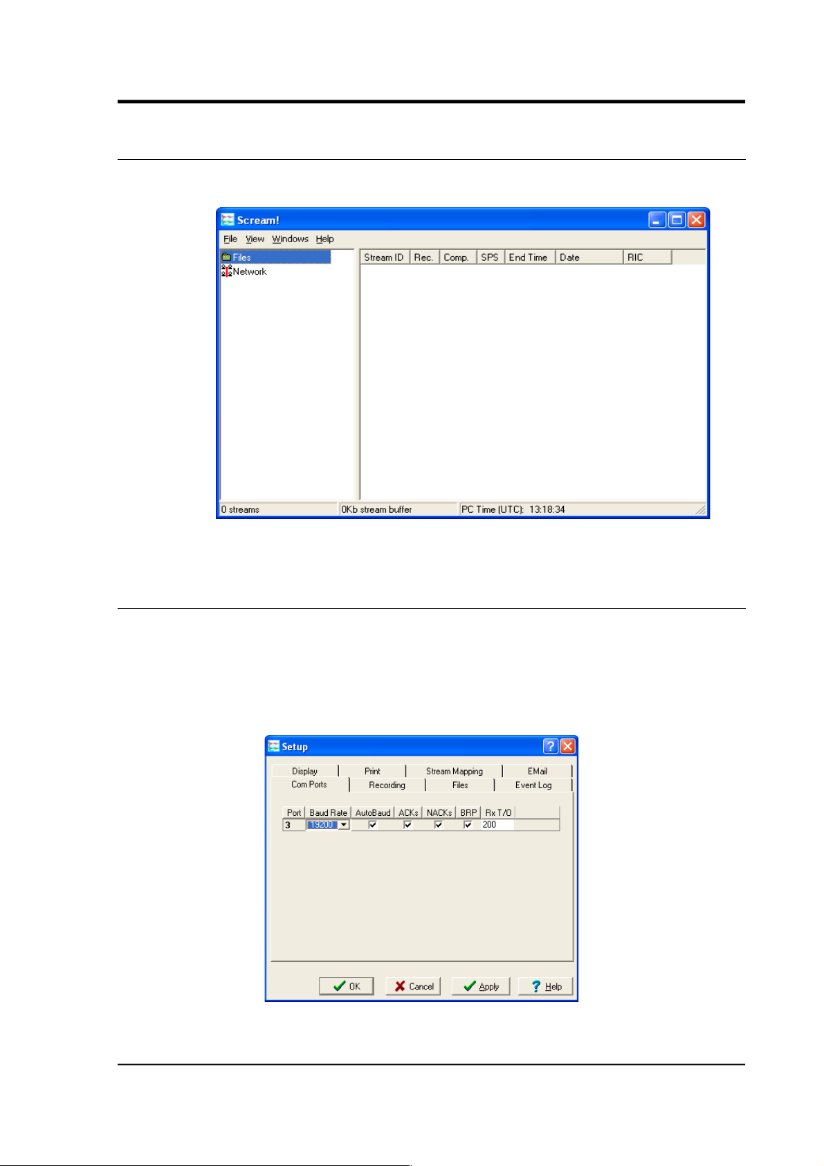
3 The main window

When you start Scream!, you will be shown an empty main window:

Scream! is now ready for you to start adding data sources.

3.1 Serial ports

1. Select File Setup…→ . If the Com Ports tab is not visible, bring it to the front.

If you are running Scream! for the first time, this window will automatically appear, together with a short tutorial.

January 2014 11

Scream! 4.5

2. The serial ports available to Scream! are listed in the table. Identify each port, and the instrument connected to it.

If you are using Microsoft Windows, the Port number corresponds to the COMn number of the serial port. If you are using Linux, Port numbers 1 – 64 refer to the built-in serial ports /dev/ttyS0 – /dev/ttyS63. Ports 65 and above refer to USB-connected serial ports beginning /dev/ttyUSB0.

A port may not be listed if it is not installed, suitable drivers are not available or if another program is using it. Scream! scans your computer for new ports each time you open the Setup window. To make Scream! scan the ports again, click the Port column heading.

3. Configure each port according to the settings of the instruments connected to them:

Baud Rate : The speed of the serial link to the instrument. The current digitiser product range defaults to 38,400 baud. Older 3-channel Güralp digitisers default to a speed of 9,600 baud; 6-channel digitisers use 19,200 baud; EAM units use a baud rate of 115,200 by default. If you do not know the baud rate of your digitiser's output port, select Auto-Detect from the drop-down menu to have Scream! attempt to detect it for you. The instrument must be producing data for this to work.

You can set all ports to the same baud rate by clicking on the column heading and choosing a suitable value from the drop-down menu.

If you are using Scream! for real time data, you will not need to change any of the remaining settings.

AutoBaud : Once connected, Scream! dynamically alters its baud rate to fit with the instrument to which it is connected. However, this can interfere with transmission over very noisy links. If you have problems, clear this box.

ACKs : Whether Scream! should send Acknowledged messages to this instrument.

NACKs : Whether Scream! should send Not Acknowledged messages to this instrument, when it detects a failure in transmission.

12 Issue K

User guide

BRP : Whether Scream! should attempt to recover dropped blocks from the instrument using the Güralp Block Recovery Protocol. You should clear this box if you are using a single-direction (simplex) communications link.

If you clear all three check-boxes (ACKs, NACKs and BRP), Scream! will never acknowledge data packets that it is sent. This is particularly useful in situations where you need to connect to a digitiser without altering the flow of data. For example, a digitiser in FIFO or ADAPTIVE mode will normally save data in Flash memory only if data packets are not acknowledged. When you come to download the saved data from such a digitiser, you should clear these check-boxes before connecting the digitiser. Doing this will ensure that incoming data continues to be saved on the digitiser, rather than transmitted to Scream!.

Rx T/O (receive time-out) : The time, in seconds, that Scream! will wait for the sender to finish transmitting a block, before assuming that it is complete. If the instrument stops transmitting in the middle of a block, Scream!'s diagnostics will detect it and request retransmission next time the instrument is on-line.

You can tick or clear all the check-boxes in a column by clicking on the column heading.

4. Click .

If any instruments are connected, data streams should now begin appearing in the right-hand portion of Scream!'s main window.

Another way to configure a serial port is to right-click on its entry in the streams list (the left-hand panel in the main window) and selecting Configure… However, you can only do this if data have already arrived through the port, making it appear in the streams list.

From this page, you can double-click on the port number of an open Com port to go directly to a terminal session on that port.

If you want to access Scream! servers on the network (i.e. EAMs, or other instances of Scream!), you will need to add the servers to the list using the Network Control window. See Section 5.1 on page 53, for more details.

January 2014 13

Scream! 4.5

Scream! will remember all the data sources you have specified on exit. When you next open the program, it will automatically try to re-establish all the connections.

3.2 The stream buffer

Scream! works by recording incoming streams into a fixed area of memory, called the stream buffer. All of Scream!'s operations work with the data in this buffer.

When you start Scream! for the first time, this buffer is empty. You can add data to it either by receiving it from local serial ports, connecting to Scream! network servers, or replaying GCF files.

Once the stream buffer is full, Scream! will start discarding the oldest data. If you have not told Scream! to record the incoming streams (see Chapter 9 on page 101), then you will not be able to get discarded data back.

You can change the size of the stream buffer in the Display pane of the Setup window (see Section 4.4 on page 48).

If you have enabled GCF recording, Scream! keeps track of the files which contain data in the stream buffer, and saves this information in a .lst file in the current recording directory (set using the Base Directory item on the Files tab of the set-up dialogue). When Scream! is restarted, it reads this file and tries to rebuild the stream buffer as it was when it was shut down. Otherwise, the buffer starts off empty as before.

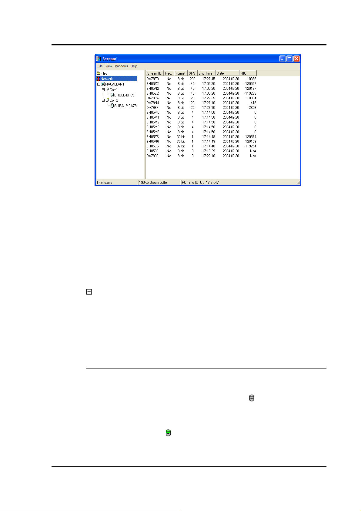
3.3 The source tree

The tree in the left panel of the main window shows all the data sources currently connected to Scream!, whether local instruments, networked instruments, or files being replayed.

Scream!'s source tree has two main parts: Files, which contains all the files you have replayed (including automatic replay: see Section 9.3 on page 112), and Network, which represents your seismic network.

Beneath Network is a list of all the network servers Scream! is connected to, plus the entry Local for your computer's own serial ports.

The next layer contains the serial ports themselves. These icons are provided to help you identify the instruments, as well as providing direct terminal access.

14 Issue K

User guide

As an example, the screen shot above shows Scream! running on a computer which is not directly attached to any instruments. It receives data from a single network source, MACALLAN1, which has two serial ports Com1 and Com2. These ports are attached to the instruments BHOLE-BH05 and GURALP-DA79 respectively: if your installation uses a CRM (Combiner-Repeater Module) or EAM connected to a serial port, several instruments may be listed under a single serial port icon.

The MACALLAN1 server icon has been “unrolled” to reveal the serial port icons. You can “roll up” icons and save space by clicking on the

box.

You can tell Scream! to ignore a particular instrument by right-clicking on its icon and selecting Ignore. When you do this, Scream! will discard any blocks it receives from the instrument. They will not appear in the stream buffer or be recorded to disk. Select Ignore again to stop ignoring the instrument.

3.3.1 Icons

Instrument icons change colour to provide you with a quick overview of the instrument's timing and mass position status:

If both halves of the instrument icon are clear , Scream! has not received any information from the instrument since the program started.

If the top half is green , the instrument has reported a satisfactory timing fix.

January 2014 15

Scream! 4.5

If the top half is yellow , the instrument has reported a gap in the timing stream. This will occur if the GPS signal deteriorates to the point where the receiver cannot keep a lock on the satellites.

If the top half is red , the instrument has not reported a satisfactory timing fix for over an hour. This will happen if the instrument has reported failures (as above), but also if it has not reported anything. If you have set the GPS system to power down for intervals longer than an hour, the icon will turn red even if the system is working normally.

If the bottom half is red , the instrument (or one of its components) is running with a mass position over 15000 counts—roughly 50% of its travel. You should re-centre the component if possible, to avoid clipping after large ground movements.

If the instrument appears as a green box , the instrument has sent status blocks to Scream!, but no data. The box represents a Güralp CRM/SAM; these modules store or forward data from other instruments, but occasionally produce status blocks themselves. If a digitiser produces a status block before any data, perhaps because you have configured very slow data rates, or are using FILING or DUAL transmission modes (see Section 8.5 on page 93), it will temporarily appear with this icon.

3.4 The stream list

If Network is selected in the source tree, the right-hand panel will list all the data streams which Scream! receives (and is not ignoring). If an entry in the source tree is selected, the stream list will only show the streams beneath that entry—selecting a serial port will only show streams from instruments connected to that port, and so on.

The columns in the table provide useful information about each stream.

Stream ID : A unique name for the data stream, being a combination of six letters A – Z and numbers 0 – 9. The first four characters of this name identify the digitiser, and the last two characters identify the individual stream.

The first four characters are set by default to the serial number of the digitiser; you can change this on the System ID pane of the Configuration Setup window (see Section 7.1 on page 77) or from the digitiser's console.

16 Issue K

User guide

The last two characters tell you the type, component, and output tap of the stream.

• Z0, N0, E0 correspond to input channels Z, N, and E of the

digitiser's SENSOR A port, continuously output through Tap 0.

• Z2, N2, E2 correspond to the same input channels, output

through Tap 1 at a lower sample rate.

• Likewise, Z4, N4, E4 and Z6, N6, E6 correspond to Taps 2 and 3.

• Z1, N1, E1; Z3, N3, E3; Z5, N5, E5; and Z7, N7, E7 correspond to

Taps 0, 1, 2, and 3 of SENSOR B, when you connect a 6-channel digitiser.

• 00 is the digitiser status stream (notice: zero sample rate).

• M8, M9, MA are slow-rate Mux channels reporting the sensor

mass positions for the Z, N, and E components (Section 7.4 on page 86).

• MB is a slow-rate Mux channel used for user input, or calibration

signals on older Güralp Systems digitisers.

• MC-F are further Mux channels, used for user input or the

digitiser's internal temperature.

• X0-X7 denote the auxiliary analogue input channel on newer

DM24 units, digitized using the same tap settings as Z, N and E.

• C0-C7 denote the same input channel, when it is being used for

an input calibration signal.

• Z, N, EG-N are the channels Z, N, E0-7, respectively, when they

output triggered data.

• IB denotes digitiser Information Blocks containing user

information. Scream! tries to interpret these blocks and automatically extracts data from them for use in WaveView windows or Matlab extensions.

• CD, BP are digitiser streams for specialised use.

Scream! can replace these designations with more helpful names if you wish: see Section 4.4.2 on page 49.

January 2014 17

Scream! 4.5

Rec. : Whether Scream! is currently recording the data stream to the computer's on-board hard disk (not the digitiser's memory). If another device on your network is recording the data stream independently of Scream!, the entry in this column will still be No. If this entry shows ERR, then there has been an error whilst writing data for this stream. Investigate the cause, then re-enable recording to clear the error.

Comp. : The compression factor of the data in the stream, expressed as the number of bits occupied by each record (8, 16 or 32 bits). This can vary block-by-block.

SPS : The sampling rate of the data stream, in samples per second. Status streams, ending in 00, do not constantly output data and have an SPS of 0. By default, the stream list is sorted in order of sample rate, with the status streams at the bottom.

End time and Date : the date and time of the most recent data, as measured by the data's own time-stamps. These are not necessarily the latest data to arrive.

RIC : The ‘Reverse Integrating Constant’. In effect this is the value of the last sample received. This is most useful for reading mass positions or other environmental streams. Status streams have a RIC of N/A.

If a stream is currently recording, on Windows the option “Explore Recording Folder” will open a Windows Explorer window at the folder where the data are currently recorded. This is useful to quickly browse to the recorded files.

3.4.1 Sorting options

Sorting options are available from the View → Sort By menu:

• Alphabetical : Strict alphabetical order, 0 – 9 then A(a) – Z(z).

• Component : Vertical components (ending Zx), followed by Nx

and Ex components, then Mux channels Mx. Within a component type, sort by the first four characters of the Stream ID.

• Instrument : Sort by the first four characters of the Stream ID.

Within an instrument, sort by tap, then by component.

• Sample Rate : Sort by sample rate, highest to lowest. Within a

sample rate, sort as Instrument.

18 Issue K

User guide

• Tap : Sort by tap (the last character of the Stream ID). Within a

tap, sort by instrument, then by component.

• Select the Reversed option to reverse any of these sort orders.

You can also sort the list by Stream ID or SPS by clicking on the relevant heading; click again to reverse the sort order.

3.5 The status bar

At the bottom of Scream!'s main window is a status bar containing summary information about Scream!'s state:

• The server address from where the data for the currently

selected instrument is being received;

• The number of different data streams currently accessible from

the window, including those that have been “rolled up”;

• The amount of memory currently being used by Scream!'s

stream buffer. You can change the maximum size of the stream buffer from the Setup window (see Section 4.4.1on page 48). If this number approaches the capacity of your computer, it may become slow and difficult to use; and

• The current time, according to the local computer (not the

timestamps of incoming data).

To disable the status bar, deselect View Status Bar → on the menu.

3.6 Viewing streams

Double-click on one of the streams to open a window for viewing the data, or right-click on it and select View…. Alternatively, make a selection of streams from the list and double-click on the selection or press ENTER.

January 2014 19

Scream! 4.5

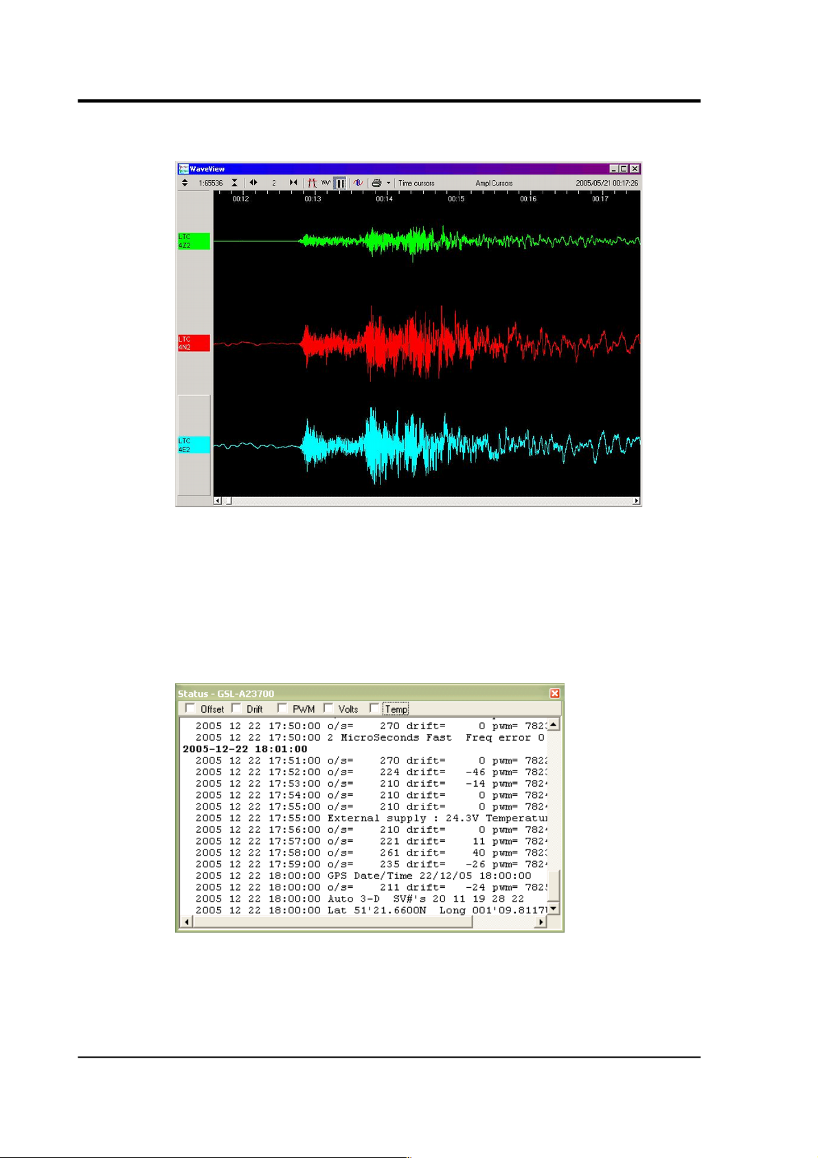
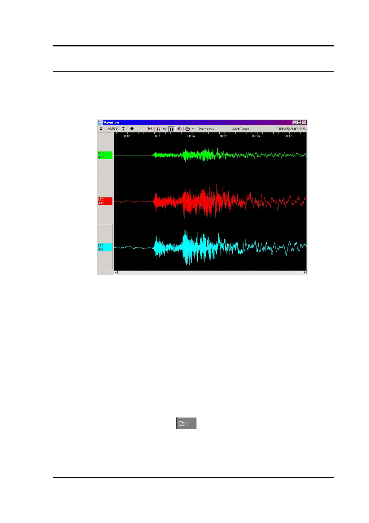
Data streams are opened in a Waveview window:

This window allows you to see real-time data coming in. You can also pause the window and examine any features held in the stream buffer. For full information on the features provided by Waveview windows, see Chapter 4on page 27.

Status streams (ending 00) consist of plain text. Double-clicking on a status stream produces the Status window:

The first blocks will give the boot message from the digitiser, including its software revision and the data streams selected for downloading and triggering. Later blocks give information on visible GPS satellites, the location of the GPS antenna and time synchronization status. Also

20 Issue K

User guide

displayed are the baud rates currently used for each channel and for the data link.

For more information on status streams and GPS, see Section 6.2 on page 66.

If you View a selection which includes both status and data streams, the status streams will be collected together and displayed in a tabbed

Status window, whilst the data streams will appear in a single Waveview window.

3.7 Connecting to instruments

Digitiser configuration and other common operations can be performed from Scream! by right-clicking on the digitiser in the source tree and selecting Configure… or Control… See Chapter 7 on page 76 and Chapter 8 on page 89 for more information.

Scream! also allows you to access the serial terminal of any connected digitiser and issue commands directly, by right-clicking on it and selecting Terminal…. See Section 6.1 on page 63 for more information about the serial terminal.

An instrument may connected to Scream! through a series of other units (NAMs, EAMs, DCMs, etc). Scream! will negotiate with each unit in turn to reach the instrument you are interested in. However, the process may take a little time.

Right-clicking on a digitiser and selecting Triggers… brings up a window describing all the digitiser triggers that have been detected. This window can also be reached from the Summary window: see section 6.3 on page 70 for more information.

3.8 Calibration data

Scream! can display data streams from displacement, velocity, and acceleration sensors in physical units. To be able to do this, it needs to know the calibration information provided with the sensor and digitiser.

Newer Güralp digitisers transmit calibration information in an information block when they reboot. When Scream! receives an information block that it understands, it automatically extracts this information and remembers it.

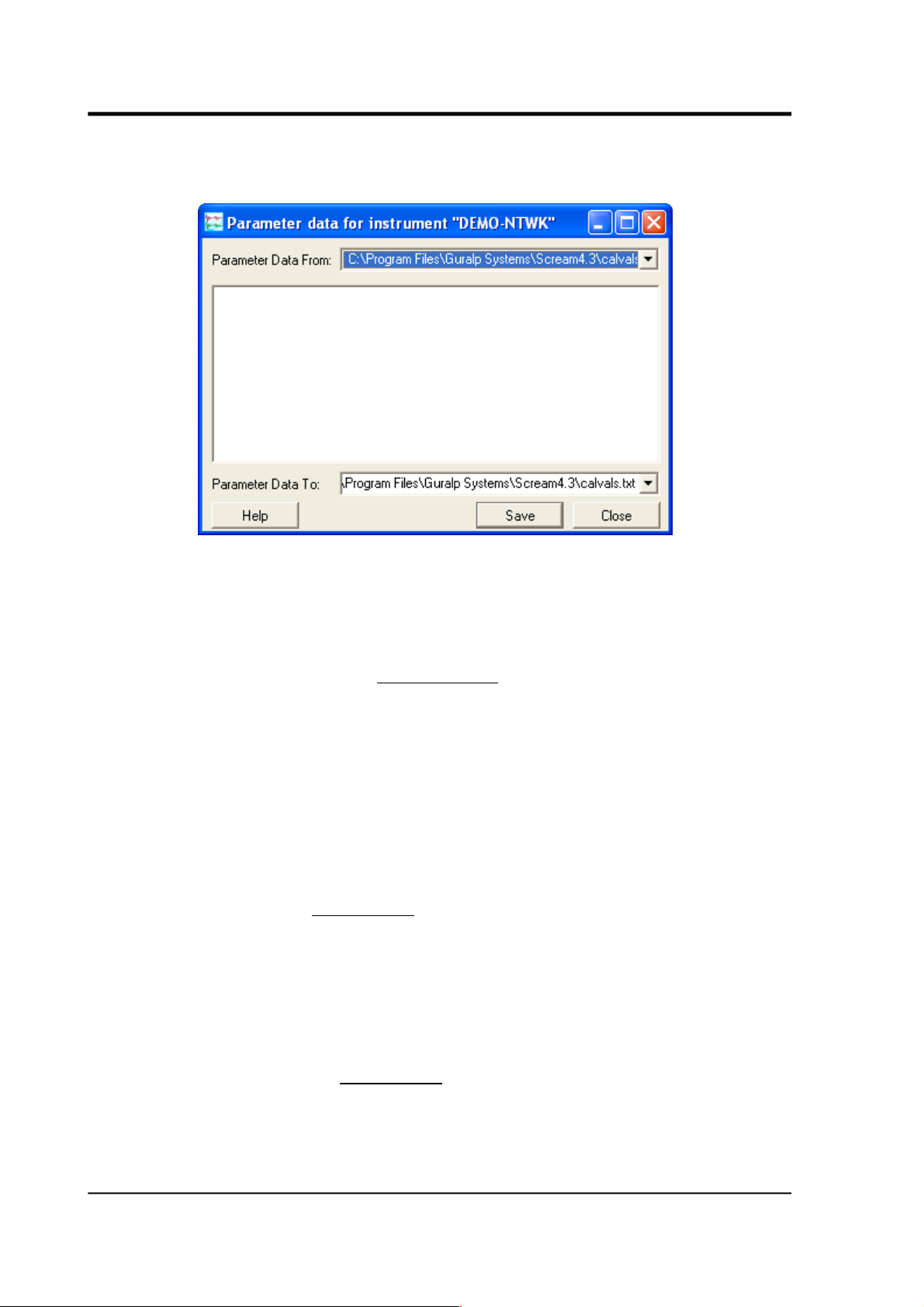
You can also enter and edit calibration information manually. Right-click on the digitiser's icon and select Calvals…. A window will

January 2014 21

Scream! 4.5

open with a text entry box. This window lets you edit Scream!'s calibration values file.

Fill in the text box with calibration information for your digitiser and the instrument connected to it, in the format described below.

• To set the serial number of the instrument, include the line

Serial-Nos=serial-number

Scream! cannot tell what instrument is connected to the digitiser. This line is provided to help you remember which set of calibration values you have used, and to provide a title for calibration graphs. If you attach a different instrument to the same digitiser, you will need to enter new calibration values to reflect the new instrument.

• To set the sensitivity of the digitiser, include the line

VPC=sensitivity

VPC stands for voltage per count, measured in units of V/coμ unt.

This is sometimes given as V/Bitμ on the digitiser calibration sheet.

• To set the sensitivity of the calibration channel, include the line

CALVPC=sensitivity

as for the other digitiser channels.

22 Issue K

User guide

• To set the value of the calibration resistor, include the line

CALRES=resistance

Güralp Systems digitisers normally use a 51 kΩ resistor (CALRES=51000).

• To set the sensor type, include the line

TYPE=model-number

e.g. 3T, 5T, etc..

• To set the response of the sensor, include the line

RESPONSE=response-type unit

Some of the values you can use are given in the table below. If none of these match the response of your instrument, please contact support for advice.

Sensor Sensor type code

Units

(V/A)

CMG-5T or 5TD, DC – 100 Hz response

CMG-5_100HZ A

CMG-40T-1 or 6T-1, 1 s – 100 Hz response

CMG-40_1S_100HZ V

CMG-40T-1 or 6T-1, 2 s – 100 Hz response

CMG-40_2S_100HZ V

CMG-40T-1 or 6T-1, 10 s – 100 Hz response

CMG-40_10S_100HZ V

CMG-40T, 20 s – 50 Hz response

CMG-40_20S_50HZ V

CMG-40T, 30 s – 50 Hz response

CMG-40_30S_50HZ V

CMG-3T or 3ESP, 30 s – 50 Hz response

CMG-3_30S_50HZ V

CMG-40T, 60 s – 50 Hz response

CMG-40_60S_50HZ V

CMG-3T or 3ESP, 60 s – 50 Hz response

CMG-3_60S_50HZ V

CMG-3T or 3ESP, 100 s – 50 Hz response

CMG-3_100S_50HZ V

CMG-3T or 3ESP, 120 s – 50 Hz response

CMG-3_120S_50HZ V

January 2014 23

Scream! 4.5

Sensor Sensor type code

Units

(V/A)

CMG-3T, 360 s – 50 Hz response

CMG-3_360S_50HZ V

CMG-3TB or 3V / 3ESP borehole, 30 s – 50 Hz response

CMG-3B_30S_50HZ V

CMG-3TB or 3V / 3ESP borehole, 100 s – 50 Hz response

CMG-3B_100S_50HZ V

CMG-3TB or 3V / 3ESP borehole, 120 s – 50 Hz response

CMG-3B_120S_50HZ V

CMG-3TB or 3V / 3ESP borehole, 360 s – 50 Hz response

CMG-3B_360S_50HZ V

CMG-3TB or 3V / 3ESP borehole, 360 s – 100 Hz response

CMG-3B_360S_100HZ V

Some English descriptions are also accepted, e.g. “120s velocity”, “100Hz acceleration” but this is not a free-format,

parsed field.

• To set the sensitivity (or gain) of the sensor components,

include the line

G=vertical-sensitivity,N/S-sensitivity,E/W-sensitivity

These values are given on the sensor calibration sheet. For velocity sensors, they are given in units of V m

-1

s (V/ms-1). The gain of an accelerometer is expressed in V m-1 s2 (V/ms-2). Because Güralp Systems sensors and digitisers use differential inputs and outputs, the sensitivity is quoted as 2 × (single-ended sensitivity) on the calibration sheet.

• To set the coil constants of the sensor components, include the

line

COILCONST=vertical-constant,N/S-constant,E/W-constant

These values are given on the sensor calibration sheet.

• To set the local acceleration due to gravity, include the line

GRAVITY=acceleration

You should give this value in ms-2, if you know it. If you miss out this line, Scream! will use a standard average g value of

9.80665 ms-2.

24 Issue K

User guide

When you have filled in all the values, click .

Any WaveView windows that are open will change to show streams in physical units. New WaveView windows will also use these units where possible.

Each digitiser System ID and serial number can have only one instrument connected to it. If you have a 6-channel digitiser with two connected sensors, you will need to make the digitiser announce different serial numbers for each one. On newer Güralp Systems DM24 digitisers, this can be done with the command SERIAL2. See the manual for your digitiser for more information.

3.8.1 Examples

The calibration information for a CMG-3T weak-motion velocity sensor might look like the following:

Serial-Nos=T3X99 VPC=3.153,3.147,3.159 G=1010,1007,1002 COILCONST=0.02575,0.01778,0.01774 CALVPC=3.161 CALRES=51000 TYPE=CMG-3T RESPONSE=CMG-3_30S_50HZ V GRAVITY=9.80122

CMG-5TD accelerometers use 1 Ω calibration resistors, and their coil constant is set to unity. Older CMG-5TD instruments, based on Mk2 digitiser hardware, do not have calibration input facilities, and thus the CALVPC entry is omitted. For example:

January 2014 25

Scream! 4.5

Serial-Nos=T5585 VPC=2.013,2.028,2.036 G=0.256,0.255,0.255 COILCONST=1,1,1 CALRES=1 TYPE=CMG-5T RESPONSE=CMG-5_100HZ A GRAVITY=9.81089

For information on the file, calvals.txt, which stores these values, see section 14.2 on page 138.

3.9 Other features

The main menu also provides some miscellaneous facilities.

Choose File Save Program State → to save Scream!'s configuration file immediately. This file is read whenever you start Scream!, and any changes are written back whenever you close it. Under Microsoft Windows, the configuration file appears as scream.ini in the c:\scream directory; under Linux, it is saved in $HOME if this variable is set, otherwise the same directory as the Scream! program file. You can change the name and location of the configuration file with a command line option (see Section 14.1 on page 137).

Choose File Application Caption… → to change the title of Scream!'s main window. This is useful if you have several copies of Scream! running on the same computer (e.g. to run multiple network services).

Choose View Stay On Top → to keep Scream!'s main window on top of all other Scream! windows at all times. Other applications may still cover Scream!'s main window.

26 Issue K

User guide

4 Waveview windows

The most commonly used features of Scream! are accessed through Waveview windows. You can open as many Waveview windows as you like, on any combination of streams; the same stream can be part of several Waveview windows at once, at several different scales.

To open a Waveview window from Scream!'s main window:

• select Window New Waveview Window… → from the main

menu;

• double-click on a stream ID in the streams list;

• right-click on a stream in the list and select View; or

• make a selection of streams and double-click the selection (or

press ENTER).

You can add further streams to the Waveview window by selecting them from the streams list and dragging the selection into the Waveview window, or by dragging them from other Waveview

windows. Dragging with held down will copy the stream from one window to another; otherwise, the stream will be moved to the

new window.

January 2014 27

Scream! 4.5

If you are running Scream! in real-time mode, and you double-click on a GCF file to view it (or open the Scream! viewer in some other way), you will have both real-time and “view” windows open. In this case, you can drag streams from real-time windows to other real-time windows, but not from these to view windows, or from view windows to other view windows. This is because the windows are handled by different instances of the Scream! program.

You can also drag streams within a Waveview window to reorder them. (If you have paused a Waveview window with the icon ( ), you will need to drag from the panel on the left, since dragging across the window will zoom in; see below.)

To the left of the stream display is a panel identifying the stream by its System ID and Stream ID, or another label if you have set one (see Section 4.4.2 on page 49). If the label is too long to read, you can resize the panel by dragging its edge across the Waveview window. You can also hide the panel this way.

4.1 Window functions

Above the stream display is a toolbar, containing icons which act on all of the streams within the window.

4.1.1 Zooming in and out

To zoom in and out vertically, click the vertical scale icons

at the top left of the window, or use your mouse wheel. The current zoom factor is shown between the icons, as a ratio of pixels to counts. Zooming in and out affects every stream in the window.

To zoom in and out horizontally, click the horizontal scale icons

, or hold down the shift-key ( ) whilst turning your

mouse wheel. The current zoom factor is shown between the icons, in pixels per second. To convert to pixels per sample, divide the zoom factor by the sample rate for the stream.

If you have a large window which takes some time to scroll, especially at a high horizontal zoom factor, Scream! may not be able to finish drawing new data before it needs to scroll again. If this happens, Scream! will delay scrolling until it can display in real time once more. To prevent this, decrease the time scale.

If you have paused the window with the icon, you can zoom into an area of interest by dragging a rectangle across the streams. Scream! displays the time span in the top right corner of the rectangle, and the

28 Issue K

User guide

number of counts in the bottom left corner. You can drag across one stream, or several; the resulting window will still include all streams.

Whilst the window is paused, you can also adjust the view start and end times by dragging the ends of the horizontal scroll bar button, at the bottom of the window.

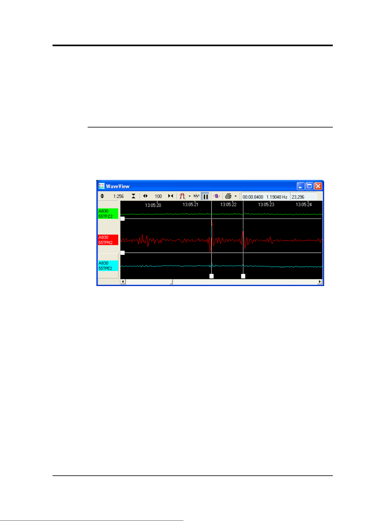
4.1.2 Making measurements

Click the Time Cursors or Ampl Cursors button to display a pair of vertical or horizontal cursors. Each cursor has a square at one end, which can be dragged across the Waveview window to measure features. If two cursors coincide, you will only be able to see the squares.

The distance between the cursors is given in the text of the Time Cursors or Ampl Cursors icon, in seconds and Hz or counts. You can have both vertical and horizontal cursors active at the same time. Because the limit of accuracy of the cursors is one pixel, you should zoom in to the range of interest before measuring.

The Ampl Cursors measure distances in counts according to the current zoom settings. However, if you have applied a scaling factor to an individual stream (see below), the Ampl Cursors do not take this scaling into account, so the measured distance will no longer be in digitiser counts; they will be in the scaled units of the stream.

To obtain the true value in counts, divide the value displayed in the Ampl Cursors icon by the scale factor for that stream, as displayed beneath its ID on the left-hand panel.

If a stream is shown with a physical unit (e.g. nm s-1), Scream! has scaled it so that the Ampl Cursors display a value in that unit. To do

January 2014 29

Scream! 4.5

this, Scream! needs to know the sensitivities of your digitiser and instrument (see Section 3.8 on page 21).

4.1.3 Printing

To print the data currently being displayed in the Waveview window,

click on the Print icon . Scream! will use the current default printer settings to print a full page view of the window, using the current amplitude and time scaling, filtering and other display options. You can print at any time, in either real-time or paused mode.

To print the same data in black and white (on a colour or grey-scale printer), click on the arrow beside the Print icon and select Page Print (monochrome) from the drop-down menu. Black and white output is more suitable for copying or faxing.

You can also set up Scream! to print automatically, or send data directly to a connected plotter. For full details on the printing options available in Scream!, see Chapter 10 on page 119.

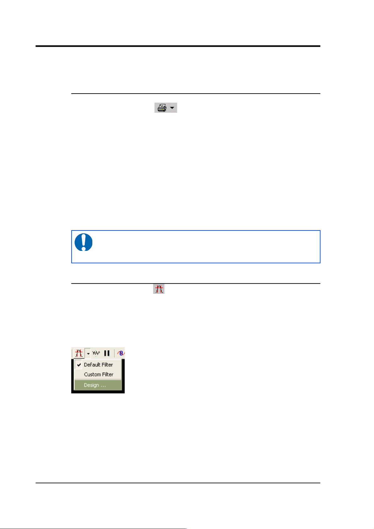
4.1.4 Filtering

Clicking the Filter icon makes Scream! apply a filter to each of the displayed streams. Click the icon again to disable the filter.

Scream! can be configured to apply different filters to each WaveView window. To select the filter, click on the arrow beside the Filter icon. A drop-down menu will appear.

• Select Default filter to apply Scream's built-in FIR bandpass

filter. The properties of this filter depend on the sample rate of the stream. Data at 1 or 2 samples per second are filtered with a 10 – 30 second pass-band, whilst data at other sample rates are filtered with corner frequencies at 0.1 and 0.9 times the Nyquist frequency of the stream. For example, the pass band for the filter applied to a stream at 100 samples per second will be 5 – 45 Hz.

30 Issue K

Note: The “print” facility is a good way to produce PDF outputs of waveforms, by using a PDF printer-driver (e.g. PDFcreator).

User guide

• Select Custom filter to activate the filter you have designed. If

you have not designed a filter, a 10 – 30 second pass band filter will be used for all sample rates.

• Select Design… to open the Filter Design window (see Section

4.3 on page 40).

• If you have saved some filter designs as presets, they will be

listed below Design…. Select an entry to switch to a Custom filter with these settings.

• If you have saved some filter designs as presets, a Delete preset

sub-menu will also appear. Select an entry in this sub-menu to

delete that filter design.

4.1.5 Paused mode

Click the Pause icon to stop the window scrolling. If new blocks arrive which contain data from the time period displayed, Scream! will add them to the window.

Whilst a window is paused, you can:

• Scroll the waveform to left and right to view all the data that

Scream! has in memory. Alternatively, hold down whilst turning your mouse wheel to scroll through the data. Because

new data are still being added to the memory buffer, the scroll bar will move slowly to the left as long as the display is paused.

• Zoom in and out to examine features in the data.

• Select data from several different streams by holding down the

shift-key ( ) and dragging:

January 2014 31

Scream! 4.5

• If the region you have selected is entirely filled with

contiguous data, the selection is shown as a solid block. If there are gaps or overlaps in any stream, the selection is shown in a hatched style.

32 Issue K

User guide

• Select data from two streams by holding down and

dragging from one to the other.

• Save data to a file by selecting one or more streams (using either

of the methods above) and choosing Save…:

Select the directory and format for the file, and click to save the data with one file for each stream (using the format shown).

Some formats support multiple streams per file. For these formats, you can select Single File to combine the streams.

The number at the top left of the selection is the number of samples from each stream that you have selected.

• Use data in a filter design by selecting a single stream and

choosing Use in Filter Design… from the pop-up menu. See Section 4.3 on page 40 for details.

• Pass data to a Scream! extension by selecting one or more

streams (using either of the methods above) and choosing the

January 2014 33

Scream! 4.5

extension from the pop-up menu. See Chapter 12 on page 130 for more details.

Click the Pause icon ( ) again to return to real-time mode. If you have changed the zoom settings, the window will return to its previous state, with the window once more following the real-time data.

4.1.6 Other icons

Click the Block Boundaries icon to display a dotted line at the end of every GCF block displayed in the window:

The number beside each line is the number of bits used to store each sample in the block. A fixed-length GCF block with 8-bit samples (which can encode differences up to ±127 counts) can store 4 times as many samples as a block using 32 bits for each one (encoding differences as large as ±4,294,967,296 counts). Clicking the icon again removes the block markers. Block markers can also show icons for re-boots and re-syncs .

Click the Zero Streams icon to set the offset of each stream in its “lane” so as to centre its mean value over the time period displayed. If you do not want a particular stream to be zeroed when you click this icon, right-click on the stream beforehand and select Locked Offset. This option is particularly useful when first setting up an instrument, since its output is often offset by a constant DC voltage.

When Scream! is used as a data viewer, the Pause icon ( ) is replaced with a Restore View icon . Click this icon to reset the time and amplitude zoom settings to their initial values, i.e. to display the entire selected data set within the window.

34 Issue K

User guide

4.1.7 Context menu

Right-clicking inside a Waveview window brings up a context-sensitive menu in two sections. The upper section of this menu contains options which affect a particular stream (see below). Options in the lower section affect the whole window:

Select Background Colour… to change the background colour for the window.

Select Label… to change the title of the window. This also changes the name of the window's entry in Scream's Windows menu, and is used on printouts (see Chapter 10 on page 119).

Select Clear Window to remove all streams from the window. This does not remove the streams from memory; you can retrieve them by dragging from Scream's main window onto the now-empty Waveview window.

Select No Caption to remove the title decoration and toolbar from the window. To maximise the screen area occupied by streams, first maximise the Waveview window, then choose No Caption. You can still use the mouse wheel or keyboard short-cuts (see Chapter 13 on page 133) to perform the actions of icons on the toolbar.

Select Duplicate to open a new Waveview window identical to the current one. (If you have renamed a stream using Stream Name Mapping, the new window will use the new name.)

Select Overlay Streams to draw all visible streams in the middle of the window, overlaid one on top of another.

January 2014 35

Scream! 4.5

This is useful if you want to compare event records from several instruments in an array. Select the Overlay Streams option again to return to the normal display settings.

4.2 Stream functions

There are also several actions you can perform on individual streams, which can be accessed from the context-sensitive menu. Each stream has its own “focus lane”, although large signals or high zoom factors may make the trace extend outside the lane.

When you move the mouse pointer over a lane, a selection box is drawn around the corresponding stream's label in the panel to the left. Right-clicking will bring up the menu options for this stream.

If you have selected Overlay Streams for the window, the focus lanes are still present even though the streams are not drawn inside them. Right-clicking in the window anywhere to the right of a stream identifier will bring up the context menu for that stream.

36 Issue K

User guide

4.2.1 Identifying streams

Every stream is identified in its icon in the left-hand panel. For more details, right-click on the stream. The topmost option in the menu displays the full network path to the instrument, including its System ID and Stream ID:

Here, a stream from a digitiser with the System ID BHOLE has a mapped name of Z (see “Stream mapping” in page 49). Right-clicking on the stream shows that the true Stream ID is DA62Z2, and that it comes from a GCF file with the name da62z2_20060112_1900z.gcf.

Selecting this option brings Scream!'s main window to the front, with the digitiser and stream selected.

4.2.2 Changing the appearance of streams

To change the colour of a stream's trace, right-click on the stream in the Waveview window and choose Colour…. Select the colour you

want to use and click .

You can also set up Scream! to use particular colours automatically according to the name of the stream, and to label them differently in the Waveview window. See Section 4.4.2 on page 49 for more details.

January 2014 37

Scream! 4.5

4.2.3 Scaling streams

To scale an individual stream, right-click on it and select Scale…:

Enter the new scale factor and click . You can scale whole instruments at a time by ticking the Copy to all components in this window box. This overrides any previous scale factor active for those streams.

If you have configured Scream! to scale streams to physical units, this box will display the scale factor Scream! is using. If you enter ed a different scale factor, it will override the factor Scream! has chosen. To return to physical units, in the scaling box, enter the word “auto”. You can also apply relative scaling by entering * and / operators. For example, entering a scaling of *2 will double the existing scale factor.

4.2.4 Viewing offsets, ranges and averages

To see the range and average value for a stream, right-click on it and select Details…. A small window will appear beside the stream giving the current offset, mean, maximum and minimum values for the data in the window, together with the Diff (difference between minimum and maximum values). The values are scaled according to the current scale factor for the stream, or to any physical unit you have selected.

To alter the offset of a stream, type a new value (in counts) into the Offset box and press ENTER. You can do this even if the stream is locked. The offset is changed for the current Waveview window only.

If you move a Waveview window, all its Details windows will move with it. You can change their relative position by dragging the title bar of each Details window.

Whilst the Details window is open, the mean value is displayed on the WaveView window as a dotted horizontal line, whilst the maximum and minimum values are displayed as solid lines.

You can also change the offset of a stream with the keyboard. With the mouse over the Details window, pressing the and arrow keys

moves the current stream up or down by one pixel, whilst and move the stream by the height of one “lane”. This feature lets you

38 Issue K

User guide

compare streams by placing one directly on top of another. The lane used for selecting the streams stays the same.

4.2.5 Spectrogram

Scream! can perform real-time spectral analysis on incoming data. To enable this feature, right-click on the stream of interest in the Waveview window and choose Spectrogram from the pop-up menu.

The vertical axis of the spectrum is linear, with the Nyquist frequency (= half the sample rate) at the top and 0 Hz (DC) at the bottom. The colouring is logarithmic, giving a large total range whilst retaining sensitivity at low signal levels.

The width of the spectrum can be changed in the Display options pane of the Setup window. The and keys adjusts the colour contrast of the spectrogram.

The spectrogram supports zooming in by dragging a selection on the frequency scale. To apply the zoom to all spectrograms in the

January 2014 39

Scream! 4.5

window, hold at the same time. To zoom out, right-click on the

frequency scale, holding , if necessary, to apply to all spectrograms.

The example below shows data from a CMG-5TD which is sensing a signal of approximately 40 Hz (green trace at the top). The Red trace shows the N/S component, with the spectrogram zoomed in once, and the blue trace where the spectrogram is zoomed in again, to the 39-40.5 Hz region. On closer inspection, it can be seen that the signal frequency is changing over time, which was not apparent from the un-zoomed green trace.

4.3 The Filter Design window

The Filter Design window allows you to alter the appearance of streams in Waveview windows by applying low-pass, high-pass or band-pass filters. Each Waveview window can have its own Filter Design settings.

40 Issue K

User guide

To open the Filter Design window, click on the arrow to the right of the Filter icon and select Design… from the drop-down menu.

From top to bottom, the window contains

• the parameters of the current high-pass (red) and low-pass

(green) filter in numerical form,

• a graph of the response of the current filter, showing the –3 dB

level and corner frequencies,

• (at bottom left) display settings for the graph, and

• (at bottom right) control buttons for the window.

4.3.1 Filter parameters

The filter parameters are shown at the top of the Filter Design window.

• Select Highpass to switch on the high-pass filter, and enter the

value of the corner frequency required in either the Hz or the Secs (seconds) box. You are not allowed to enter a value of 0 in

either box.

January 2014 41

Scream! 4.5

While the cursor is in one of the frequency boxes, pressing the

and keys will nudge the corner frequency up and

down.

Alternatively, change the corner frequency by clicking on the graph with the left mouse button. If the low-pass filter is active, and you click to the right of the low-pass corner, both frequencies will be moved.

If the frequency you want is not shown in the window, it may be above the Nyquist frequency for the currently-selected sample rate. Change the value in the n sps box at the bottom left and try again.

Change the order of the filter by entering a number in the nth Order box.

• Select Lowpass to switch on the low-pass filter, and enter the

value of the corner frequency required in either the Hz or the Secs (seconds) box.

Alternatively, change the corner frequency by clicking on the

graph with the right mouse button. If the high-pass filter is active, and you click to the left of the high-pass corner, both frequencies will be moved.

Change the order of the filter by entering a number in the nth Order box.

42 Issue K

User guide

• To create a band-pass filter, select both Highpass and Lowpass.

Enter values into the text boxes, or click in the graph with the left and right mouse buttons to set the two corner frequencies.

When both filters are active, the individual filters are shown on the graph in light blue.

• Enter a value in the Gain (dB) box to change the gain of the

filter.

In the example above, the overall gain of the band-pass filter has been set to 10 dB. This is done by applying a 5 dB gain to each of the component filters. As a result, the light blue traces appear 5 dB below the dark blue trace.

January 2014 43

Scream! 4.5

4.3.2 Viewing spectra

You can overlay the power spectra of up to two streams on the frequency graph. This is intended to help you design filters for specific events by focussing on the frequencies at which the event has significantly more energy than the background noise.

To design a filter for a specific event:

1. View the relevant stream in a Waveview window and click the Pause icon ( ). Zoom in to a time period where the stream is quiet.

2. Holding down the shift-key ( ), select a single stream across this quiet time range. Choose Use in Filter Design… from the

drop-down menu. The Filter Design window will appear, with the spectrum of the background noise overlaid.

44 Issue K

User guide

If you do not see the Use in Filter Design… option, check that only one stream is selected.

3. Leaving the Filter Design window open, switch to the Waveview window and view the event of interest.

4. Holding down the shift-key ( ), select data from the same stream during an event. Choose Use in Filter Design… from the

drop-down menu. A dialogue box will open asking you if you want to replace the previous spectrum or add to it.

Click . The spectrum of the event will be overlaid on the background noise spectrum, in a lighter shade.

You can now click in the graph to move the filter's corner frequencies to suit the event.

January 2014 45

Scream! 4.5

5. If you want to view the spectrum of a different event, follow steps 3 – 4, choosing Yes when you are asked if you want to overlay the spectra. The old event spectrum will be replaced with the new one.

6. If you want to change the background spectrum, follow steps 1 – 2 and choose No when you are asked if you want to overlay the spectra. The old event spectrum will be erased, and the background spectrum will be replaced with the new one. Now follow steps 3 – 5 to overlay the spectrum of events as desired.

4.3.3 Display options

The icons at the bottom left of the Filter Design window change the properties of the graph.

• The Log/Lin selection box allows you to choose a logarithmic or

linear time axis. (The magnitude axis is always displayed in dB, and is therefore logarithmic.)

• Enter a value in the n sps box to display a time range suitable

for streams at that rate. The graph displays a four-decade frequency range, up to the Nyquist frequency (i.e. half of the sample rate).

• When power spectra are being displayed on the graph, there is

an additional selection box to the right of the Log/Lin icon.

The power spectrum calculation uses the Welch averaging periodogram algorithm. This algorithm produces frequency graphs by splitting the range into windows of a certain size.

46 Issue K

User guide

You can alter the size of window used by changing the value in this selection box.

Using a smaller window size produces a smoother graph, at the expense of losing information about lower frequencies. To examine lower frequencies, you will need to increase the window size; however, doing this will increase the noise visible at high frequency.

4.3.4 Pre-sets

When you are happy with your filter design:

• Click to apply the filter to the Waveview window and

close the Filter Design window.

• Alternatively, click to apply the filter and leave the

Filter Design window open.

Ticking the Auto-Apply check-box makes the Filter Design window apply immediately any changes you make to the filter. Since applying a filter may take some time, you should not tick Auto-Apply if you are viewing a large amount of data.

To save the design in Scream!'s configuration file, click and enter a name for the filter. You can now select the filter from the drop-down menu next to the Waveview window's Filter icon.

January 2014 47

Scream! 4.5

4.4 Display options

There are a number of Scream! set-up options which affect how Waveview windows are displayed.

4.4.1 Display set-up

To change default display options for new Waveview windows, choose

File Setup… → from the main menu and click on the Display tab.

Stream Buffering : You can change the size of Scream's stream buffer

by altering the value and unit in these boxes. Scream! will discard any data older than this. If you want to record data to your computer's hard disk, you should use the Recording and Files panels; when you enable recording on a stream, any data in the stream buffer will be included in the recorded files. Scream! can also play back recorded GCF files (see Chapter 9 on page 101).

Status Font : Click to change the font used in status streams. The change comes into effect on new and existing Status

windows as soon as you click click or .

Waveview Defaults : Allows you to take the default properties for new Waveview windows from a window already on the screen.

Click and then on the window you wish to copy. When you

48 Issue K

User guide

click or , new Waveview windows will have the same horizontal zoom factor, filter and block boundary options, background colour, and time/amplitude cursor state as are currently in place on that window. The vertical zoom factor is used only for new, blank Waveview windows, since Scream! automatically chooses a suitable factor if it can.

Colour-coded Components : When this box is ticked, Scream! will look for stream names ending Zn, Nn, En or Xn and automatically display them in the colours shown. To change the default colours, click on the boxes. Other streams are assigned a colour in rotation as they arrive. To define more specific colour defaults, you can use stream mapping (see below).

Spectrogram : Alter this value to change the height of spectrograms displayed in Waveview windows, in pixels. When you click or , newly-drawn spectrograms in all Waveview windows will

use the new height. Pressing will cause a Waveview window to be redrawn, as will resizing it, changing the zoom factor or using other

buttons on the toolbar. Moving a window, or obscuring it and then revealing it, may or may not cause a redraw, depending on your operating system.

Units : Scream! can automatically scale new WaveView windows to physical displacement, velocity, acceleration units using sensitivity information you provide (see Section 3.8 on page 21). To enable this feature, first edit the calibration values for your digitiser, then select a suitable unit from the Displacement, Velocity, or Acceleration drop-down lists.

Once you have done this, streams from the digitiser will be scaled automatically. Other instruments will default to displaying in counts.

A simple linear scaling algorithm is used, which does not take into account the response profile of the instrument, although where the instrument has a flat response in the pass-band, it is normally a sufficient approximation. For accelerometers, this is usually sufficient to be useful.

4.4.2 Stream mapping

You can tell Scream! to look for streams with a particular Stream ID, and to display them in Waveview windows with their own colour and label. This is done from the set-up window. As with all set-up options, Scream! will remember any mappings you create, and restore them next time you run the program.

January 2014 49

Scream! 4.5

To create a new stream mapping:

1. From Scream!'s main window, choose File Setup…→ . Switch to the Stream Mapping tab.

2. Tick Use Stream Name Mapping. The pane will change to show the new options:

3. Click and fill in the Stream ID you want to change, the new label and colour.

The label can be any length, but may not contain any of the characters

50 Issue K

User guide

\ / : * ? " < > |

because these characters are not allowed in DOS or Windows file-names.

4. Click . In this example, new Waveview windows containing the DEMOZ2 stream will now automatically show it in the new colour, and with the label My 6TD vertical. The new label is also used in the main window, on printouts and in the file-names of recorded data streams (if your format specifier includes the Stream ID). Identifiers inside exported files will still use the original Stream ID.

Waveview windows which are already open will not change until they are refreshed (e.g. by resizing or zooming them, or by

pressing ).

You can edit an existing mapping by double-clicking on its entry in the table, or by selecting it and clicking Edit…. To change the default colour only, click the colour panel under Col in the table.

To delete a stream name mapping, select it and click .

January 2014 51

Scream! 4.5

Clicking enables you to import a scream.ini file from another Scream! installation and extract the mappings from it. This is useful when you want to use a standard set of names and colours for several Scream! installations.

52 Issue K

User guide

5 Networking

You can use Scream! to access the data from a digitiser (or from another copy of Scream!) from anywhere on a local or remote network.

Once a network connection is set up, Scream! can act as a server to provide data to other computers running Scream! or archival programs. To view the currently active Scream! network connections, select Network Control from the Window menu of the main window:

Scream! uses a single local port to communicate with all servers and clients. You can change the number of this port by editing the Port used for all network communications box. You may need to do this if you want to run several instances of Scream! on the same computer.

5.1 My Client

The standard mode of transmission in Scream! uses UDP. Blocks of data are received in UDP packets, which are shown in the Block Rx pane. UDP does not guarantee that data will be successfully received. If data are lost and subsequently recovered, a diagnostic message will appear in the Control pane.

Scream! has two methods for serving data. In the first, Scream! keeps a list of clients which need to be provided with data. This method is known as “server push”:

January 2014 53

Scream! 4.5

All data received on the server's serial ports will be sent to these clients automatically. On the client side, to begin receiving data, you should simply tick the Receive Data box on the My Client tab. No other action is necessary. If your client is behind a firewall, you will need to unblock the UDP port at the client side.

See Section 1.1.4 on page 56 for details of how to set up the server.

Additional clients may also request data from the Scream! server. This method is known as “client pull”:

The requests are placed in UDP packets which the server can recognize. If your server is behind a firewall, you will need to unblock the UDP port at both client and server side.

To request data from the server by this method:

1. Switch to the My Client tab.

2. Tick Receive Data to start Scream! listening.

3. Right-click anywhere in the Servers list box, and select Add UDP Server…. Enter the IP address (in numerical form or as a hostname) followed by a colon (:) and the port number on which the server waits for requests; e.g. 192.168.42.98:1567.

4. Test communications by right-clicking on the newly-added server, and selecting GCFPING. A message appears in the Control pane logging the ping being sent. If communication is good and the server is enabled for client requests, you will receive a GCFACKN message (acknowledgement) from the server. This will also appear in the Control pane.

5. Request data by right-clicking on the server and selecting GCFSEND:B from the pop-up menu (B for big-endian byte order). Streams should soon begin to appear in Scream!'s main window.

54 Issue K

User guide

6. To stop the link, right-click as before and select GCFSTOP from the pop-up menu. If you do not GCFSTOP, the server will continue to transmit to a client that is no longer listening. You should ensure that the server replies with a GCFACKN message: If an acknowledgement does not appear in the Control pane, repeat the GCFSTOP command.

Scream! automatically issues a GCFSTOP to all connected servers when it exits.

The steps above can be repeated as many times as necessary to pull data from several servers. Scream! remembers all the network settings when it exits, and automatically tries to reconnect when you start it again.

5.1.1 TCP clients

Clients can also make a TCP connection to Scream! and request data. Using this method, block re-transmission requests are delegated to the network protocol stack but there is a significant overhead involved in keeping the connection active.

Clients using TCP can access the server by its host name as well as by its IP address. This is useful for installations where the IP address may change.

5.1.2 Multicast clients

Multicasting is a feature of TCP/IP which allows you to send network packets to several clients at once. These are most often used on local networks. Multicast servers use addresses between 224.0.0.0 and

239.255.255.255. CMG-EAMs and CMG-NAMs, for example, always listen on the multicast address 239.193.15.67. (Mnemonic: 239.193 is in the privately-assignable block and 1567 is the default scream port.)

When you Add a multicast server, right-clicking on its entry in the Servers list box pops up a menu with Connect and Disconnect options in place of the GCFxxxx commands.

Selecting Connect instructs Scream! to join the multicast group with that address. If the server is running, data should begin appearing immediately.

Selecting Disconnect makes Scream! leave the multicast group. You can be in several multicast groups simultaneously, and join or leave each one independently of the others.

January 2014 55

Scream! 4.5

5.2 My Server

Scream!'s server transmits data over the network via UDP. To prevent network loops, separate options are available to serve local data (from directly connected instruments), or to relay data that were received by the Client (Transmit data from Network).

The list of clients to which Scream! is currently sending data is shown in the Clients table at the top of the My Server pane. Block-by-block details of the data being transmitted are shown in the Block Tx pane. Other server operations are reported in the Control pane to its right.

Both “server push” and “client pull” clients are listed in this pane. You can see which clients are using which method by looking in the Time-out column. When a pull clients requests data, its time-out is reset, and then starts counting down toward zero. If a pull client's time-out value reaches zero, Scream! assumes it has stopped listening and removes it from the list. On the other hand, push clients do not have a time-out, because Scream! will always try and transmit to them. Thus, clients using pull have a time-out figure listed in this column, whilst pull clients are shown with the entry None.

To start a server and listen for pull requests from clients, tick the Transmit data from local Com Ports check-box on the My Server pane. No other action is necessary. If your server is behind a firewall, you will need to unblock the UDP port at the server side to receive these requests.

To push data to a particular client:

• Switch to the My Server pane.

• Tick the Transmit data from local Com Ports box.

56 Issue K

User guide

• Right-click anywhere in the Clients list box and select Add…

Enter the IP address (or DNS name) and port number on which the server is waiting for requests, separated by a colon : (e.g.

192.168.42.98:1567)

You can add any number of clients, including broadcast addresses and multicast groups. If you want to broadcast or multicast UDP packets, you should obtain suitable addresses from your network administrator.

• To broadcast to all connected computers, use the IP address

255.255.255.255.

• To restrict broadcasts to a particular subnet, use the broadcast

address for that subnet: for example 192.168.60.255:1567 will broadcast data on port 1567 to all clients on a

192.168.60.0/24 subnet – i.e. those with IP addresses beginning 192.168.60.

• To send data to all instances of Scream! in a multicast group,

use a multicast IP address. The address range from

239.255.0.0 to 239.255.255.255 is available for local networks, and that from 239.192.0.0 to 239.195.255.255 for organisation-level networks. Most other multicast addresses on the Internet must be specially registered.

The server will automatically start transmitting.

• To send data to another Scream! running on the same computer,

use the IP address 127.0.0.1.

To send data to more than one Scream! running on the same computer, use the local broadcast address 127.0.0.255, or set up a multicast group.

You can limit the data Scream! sends by setting a maximum sample rate for transmitted streams. Enter a value into the x sps transmitted block limit box to set this rate. This is useful if your network connection is slow or congested. The default value is 1,000 samples per second.

For example, if a digitiser is configured to generate 4 samples per second and 100 samples per second continuous data, you could monitor the data remotely over a low-bandwidth network by setting this value to 10. The high-rate data can still be recorded on the server if Scream! is so configured (see Chapter 9 on page 101) but they will not be sent over the network.

January 2014 57

Scream! 4.5

Setting this value to zero suppresses all data streams, but still transmits status streams.

You can configure Scream! to let remote clients configure the instruments connected to your computer. To enable this, select Allow remote access to Com Ports. If you are concerned about security, or there are potential problems from outside interference, disable this option. You should never enable this option if you are transmitting data across the Internet.

To alter the IP address or destination port of a client, right-click on it and select Edit…. Enter the new IP address and port as for Add…, and

click

To remove a client from the list, right-click on it and select Delete.

The Scream server must store a history of the data transmitted in case the client does not receive all data. Scream! versions prior to 4.5 used a memory buffer for this purpose, which was relatively small, and only offered a small amount of backfilling to the clients.

Starting with Scream! 4.5, the user can specify a backfill buffer that is stored on disk, and can thus be very large. The Server Buffer page allows the configuration of the size and location of this disk-based buffering.

If the disk-based buffering is not enabled, Scream! will use the memory-based buffering which was used in previous versions.

58 Issue K

User guide

5.3 Server Buffer

It is recommended that the user ensures there is sufficient disk space available on the drive selected to hold the buffer. The buffer size can be specified in either time (Days, Weeks, Years), or in terms of disk usage (Mb/Gb/Tb).

5.4 Gap recovery

In addition to the normal UDP data protocol, Scream! has facilities for attempting to recover missing data. When Scream! receives a block of data that indicates a gap, it connects to the server over a TCP link (from the same port). Once this connection is made, Scream! requests the missing data and, if they are available, the server transmits them over the TCP connection. The UDP data stream is unaffected.

If you are using a firewall on either side of the connection and want Scream! to be able to recover missing data in this way, you will need to unblock the relevant port for both UDP and TCP traffic.

5.5 Retrieving data over dial-up links

Scream! can manage the retrieval of data from your installation using modems attached to your local PC. This feature is intended for use in conjunction with the triggering capabilities and Flash recording modes of Güralp digitisers.

1. Click File Setup… → on Scream's menu bar. Select the Com Ports tab.

January 2014 59

Scream! 4.5

You will see a list of all the serial ports available on your computer. This example shows a computer with a single serial port, COM3, which is attached to a modem.

2. Make sure the baud rate and other flags are set up correctly for the modem, and click .

60 Issue K

User guide

3. Enter the telephone number of the remote modem. If you want to contact several remote installations in turn, list their numbers, one per line.

4. In the right-hand panel, tick Every (12) hours, and set the value to 12.

5. Tick the Limit each call to… box, and enter a suitable call length. Scream! will also hang up if it fails to receive any data for a specified length of time.

Ensure that you allow enough time in each call to download all the new data given the sample rates and baud rate that you have chosen. For example, if the modem connection can achieve 19200 baud, then a station outputting continuous 200 samples/s data for 3 components would require a continuous connection to collect all the data. If the data rate were only 20sps, then the modem would only need to be connected for 10% of the time (e.g. a 6-minute call every hour).

6. If the local modem needs extra commands, you can add these under Additional Modem Settings. Some useful commands are Q1 to enter “quiet mode”; E0 to turn off local echo, and S0=1 to turn on the auto-answering facility. Modem commands normally start with the attention sequence AT; Scream! adds this sequence automatically, so you do not need to enter it in this box.

Some modems have dip-switches which allow you to set permanent defaults for each command. These can be useful for autonomous installations, when you want to ensure that the modem does not enter an unrecoverable state.

7. When all the settings are correct, tick the Active check-box and click to start polling.

8. To switch off polling without losing your settings, clear the Active check-box.

If you have more than one modem attached to your computer, you can set each one up with a different set of numbers and polling times. You might want to do this if:

• you want to collect data from several stations simultaneously; or

January 2014 61

Scream! 4.5

• using several modems allows you to reduce call charges (e.g.

you might use a cellular modem to contact installations on GSM networks, and a standard PSTN modem to contact those on land lines).

You can have up to 99 modems collecting data simultaneously, each with an unlimited number of scheduled dial-up times and telephone numbers. Scream! will remember all the settings when you exit.

62 Issue K

User guide

6 Supplementary windows

Aside from the main window, Waveview windows and Network control window, Scream! includes facilities for monitoring status streams, the status of your network, the integrity of incoming data, and for accessing the serial console of attached digitisers.

6.1 Terminal windows

Scream! can open a terminal session with any connected digitiser or EAM, either using a serial link or over the network (if the server permits it: see Section 5.2 on page 56).

6.1.1 Communicating with instruments

To open a terminal session with an instrument, right-click on its entry in the left pane of Scream's main window and choose Terminal… from the pop-up menu:

Scream! automatically negotiates with any other Güralp devices or software in the chain until it reaches the one you want to contact, and then attempts to place the target digitiser in command mode. If this

fails, press + in the Terminal window to enter command mode manually.

If you see an ok prompt as shown below, the digitiser is ready to receive commands. Otherwise, press ENTER to display a prompt. You can now type terminal commands into the window.

January 2014 63

Scream! 4.5

The + and + arrow keys let you browse through the history of typed commands. This history is common to all

Terminal windows, so you can easily (for example) send the same command to several digitisers in turn.

To begin capturing a session in terminal mode, including every command you type as well as the instrument's response, right-click in the Terminal window and select Capture to File…. All subsequent actions will be saved to the file you select. Capturing stays in effect through digitiser restarts and, also, if you close Scream! and restart it later. The capture file's name is displayed in the caption of the Terminal window.

To send a file to a digitiser, right-click in the Terminal window and select Send File…. This can be used to read in lists of commands that you have prepared; for example, to set up a number of digitisers identically. It is also used to update a digitiser's firmware. For details on how to set up firmware transfers, refer to the documentation for the relevant digitiser.

To close the connection, close the Terminal window. Scream! will automatically instruct the digitiser to start transmitting data. If the digitiser begins transmitting data whilst the Terminal window is still open (e.g. because you have issued the close or go command, or because of a time-out), the window will close automatically with the message Terminal session closed by instrument.

64 Issue K

User guide

6.1.2 Macro commands

The Terminal window provides icons for the keys – , which can be programmed with commonly-used commands (“macros”). To

define such a macro, right-click on an Fn icon, and enter the command (or commands) in the text box.

You can enter these commands by

• left-clicking one of the Fn icons in the Terminal window,

• pressing the corresponding function key whilst the Terminal is

open, or

• right-clicking on the digitiser's entry in Scream!'s main window,

and selecting the command from the drop-down menu. Scream! will automatically start a terminal session with the instrument, send the command and then close the link.

Scream! remembers all your macro settings when you close the program.

6.1.3 Direct connections

You can also open a terminal session directly to your computer's serial ports or over a network. This is useful for communicating directly with modems, or with third-party equipment.

To do this, select File Terminal…→ from Scream's main menu:

• To make a serial connection, choose Direct Serial as the Link

Type, select the name of the serial port you want to use, and

January 2014 65

Scream! 4.5

check that it has the expected baud rate. If it does not, you can change it in the Setup window (see Section 3.1 on page 11).

Click .

• Scream! servers can provide access to their own serial ports over

the network. To connect to the serial port of a remote Scream! server, choose Remote Serial and fill in the IP address of the remote computer, together with the port name or number.

Click .

You will need to enable serial access on the Scream! server to use this feature. In the My Server tab of the Network Control window, tick Allow remote access to Com ports.

If your Scream! server is a CMG-EAM, you will need to ensure that the “Disable terminal access” check-box is not ticked in the server configuration dialogue. Similarly, if your Scream! server is a DCM running native firmware (i.e. not upgraded to run Platinum firmware), you will need to set the option datatransfer.scream.server.allowserialaccess to yes.

This option is most useful for accessing serial ports on a remote computer which is not producing GCF data. If a remote port does emit GCF data, it will appear in the source tree as normal, and you can open a session with it by right-clicking and selecting Terminal….

• To connect over a TCP/IP terminal link, either to a remote

Scream! server or to a TCP terminal device (e.g. a serial to network converter), choose TCP/IP and fill in the IP address of

the remote computer. Click .

The terminal window will then open as described above.

6.2 Digitiser status streams

All Güralp digitisers have a separate stream for reporting information about the system, such as their GPS and time synchronization status. This status information is in plain ASCII text format.

To see a Status window for any digitiser, double-click on the Stream ID xxxx00. This stream always has a reported sample rate of 0 samples per second.

During boot-up, each unit reports its model type, firmware revision number, its System ID and serial number. This information is

66 Issue K

User guide

followed by the number of resets that have occurred and the time of the latest reboot from its internal clock. The following lines report the current configuration of the unit's sample rates, output taps, and baud rates. A typical digitiser re-boot status message looks like this:

The system will produce a similar status message whenever it is powered up and whenever you reboot it (for example, after changing its configuration).

6.2.1 GPS

If a GPS unit is fitted, its operational status is reported on reboot and the behaviour of the time synchronisation software will also be shown.

From a cold start, GPS will initially report No GPS time together with its last position (taken from the internal backup). All messages from the GPS that involve a change of its status are automatically reported. Repeated status messages are not shown to avoid unnecessary clutter.

January 2014 67

Scream! 4.5

A typical GPS status report from a DM24 digitiser looks like this:

This report shows the satellites the system has found, along with their corresponding signal strengths.

If the system has not been moved from its previous location, it should be able to find enough satellites to obtain an accurate GPS time fairly quickly; if the GPS receiver has difficulty finding satellites, there may be a delay of several minutes before a new message is displayed.

Before beginning, the digitiser's internal time synchronisation software will wait for the GPS unit to report a good position fix from at least three satellites, for at least six consecutive messages. Messages are normally received every 10 to 20 seconds.

The system will then set the internal clock and re-synchronise the Analogue to Digital Converters so that the data are accurately time-stamped to the new reference. Any data transmitted up to this point will be stamped with the time from the internal backup clock, which is set to the new accurate time at the end of this process. The re-synchronisation will result in a discontinuity in the data received.

From this point, the control process will attempt to keep the internal time-base synchronised to the GPS 1 pulse-per-second (PPS) output, by adjusting a voltage-controlled crystal oscillator. First it alters the voltage control to minimise the error. Next it attempts to minimise both the “phase error” (i.e. the offset between the internal 1 Hz signal and the GPS) and the drift (the frequency error relative to GPS). During the control process the system reports the measured errors and the control signal applied, as a PWM (Pulse Width Modulation) value.

During the initial, coarse adjustment stage, only the coarse voltage control is used and no drift calculation is made. If the system is operating in a similar environment to that when the system was last powered (most importantly, the same temperature), the saved control

68 Issue K

User guide

parameters will be appropriate and the system should rapidly switch to the ‘fine’ control mode. The system reports its control status and parameters each minute, with error measurements given in nominal timebase units. In a stable temperature environment, the system should soon settle down showing an offset error of only a few thousand (average error < 100 microseconds) and a drift rate under

100 counts (< 1 in 10-6).

6.2.2 Graphing status information

Newer Güralp digitisers output a status block every few minutes giving information about the GPS status, ambient temperature, etc:

Scream! can automatically extract measurements from these messages and show them in graphical form. For each field Scream! finds, a check-box is displayed at the top of the Status window. In the example above, Scream! has found Offset, Drift, PWM, Volts (i.e. user input) and Temp (temperature) fields in the status messages. Not all digitisers output all of these fields, so some of these check-boxes may not be present.

To display any or all of these fields in graphical form, tick the check-box(es) for the field(s) you want to examine:

January 2014 69

Scream! 4.5

You can resize the Status window, or drag the bar between the graphs and the block display area, to see the graphs in more detail.

6.3 The summary window

This window provides at-a-glance state of health information about all instruments on your network. To open it, choose Windows → Summary window from Scream!'s main window.

Every instrument known to Scream! is listed in this window, with coloured icons representing their timing, mass position and data flow status. The window also reports how many triggers have been communicated to Scream! in status blocks. To make Scream! forget all

this information and start afresh, click . This will not remove streams from the main window, the Waveview windows or the stream buffer.

In the leftmost four columns, each entry is a coloured rectangle with a border. A grey rectangle indicates that no relevant data have been received from the instrument since Scream! was started. Green indicates that this measurement is satisfactory; yellow indicates that some attention may be necessary, and red indicates that there is probably a problem.

If a box has a coloured border, an unsatisfactory reading has been received since the last reset, but the status has since improved. Thus, if a box goes from yellow to green, the border will be coloured yellow until you reset. If the same box subsequently turns red momentarily and then returns to yellow or green, the border will change to red.

70 Issue K

User guide

6.3.1 Timing

This column details the instrument's GPS timing status. The colours are the same as those used for the top half of the instrument's icon in the main window. Double-click on a column entry to see the status messages coming from that instrument.

Grey : Scream! has not received any GPS information from the

instrument since the last reset.

Green : The instrument has reported a satisfactory GPS timing fix.

Yellow : The instrument has reported a gap in the timing stream. This

may occur if the GPS signal deteriorates to the point where the receiver cannot keep a lock on the satellites.

Red : The instrument has not reported a satisfactory timing fix for over

an hour. This will happen if there have been gaps in the signal (as above), but also if it has not reported anything. If you have set the GPS system to power down for intervals longer than an hour, the icon will turn red even if the system is working normally.

6.3.2 Mass position

This column details the instrument's mass position status. Double-click on a column entry to open a Waveview window on the instrument's mass position channels.

Grey : Scream! has not received any mass positions information from

the instrument since the last reset.

Green : The instrument has reported satisfactory mass positions (all

components < 25% of full scale).

Yellow : One or more components are reporting mass positions

between 25% and 50% of full scale. Most instrument types will still function normally, but the masses should be re-centred when it is next convenient.

Red : One or more components are reporting mass positions over 50%

of full scale. Most instrument types will still function adequately, but the masses should be re-centred as a matter of urgency.

January 2014 71

Note: some instruments must be switched to one-second response mode for these channels to give meaningful data.

Scream! 4.5

6.3.3 Age

This column records the time the instrument last sent data to Scream!.

When a data block is received, the box turns green. Over the next two minutes, if no more data are received, the box gradually changes through shades of yellow, to orange, and finally red.

If more than two minutes pass before the next data block is received, the border of the box will change to red to alert you that a suspicious gap in data has been detected. If you do not expect real-time data from this instrument, or you are using low sample rates exclusively, you may allow this column to turn red. For example, a 1 sample per second stream will transmit a block only once every four minutes under quiet conditions.

Double-click on a column entry to select the instrument in Scream!'s main window.

6.3.4 Errors

This column records the number of corrupted blocks Scream! has received. A corrupted block is one whose checksum does not match the data, or which fails one of Scream!'s integrity checks. To see which checks are failing:

• Open a ViewInfo window on the suspect stream, where

erroneous values are shown in red (see Section 1.1.4 on page

74).

• Alternatively, double-click on the column entry to open the error

log file (if you are recording one) in Notepad or an xterm.

The meaning of the colours is as follows:

Green : Fewer than two corrupted data blocks have been received in

the last minute, or the window was reset less than a minute ago.

Yellow : between two and ten corrupted data blocks have been received

in the last minute.

Red : More than ten corrupted data blocks have been received in the

last minute.

6.3.5 Triggers

This column records the number of times the digitiser has sent a trigger status message since Scream! was started. New triggers are

72 Issue K

User guide

coloured in green; when you Reset window, the green shading will disappear, but the number will remain.

Double-clicking on a column entry opens a window with details of the trigger events.

The top half of the window lists all the trigger events, with information extracted from each trigger's status message. The full status message is reported in the lower half.

Double-clicking on an entry in the table (or selecting it and pressing ENTER) opens a paused Waveview window containing all the streams from the digitiser which triggered, for the time period of the trigger. This time period is marked with the Time Cursors to show the duration of the event.

If you have instructed the digitiser to record pre- or post-trigger data, Scream! will attempt to include these as well. If two triggers from the same digitiser overlap, Scream! may show both triggers in the Waveview window, because the point where one trigger ends and the next begins is essentially arbitrary.

Scream! can only display data which is still in its stream buffer. If the buffer is full and the data have already been purged, double-clicking on a trigger will show a blank window. To view the data, you will need to retrieve it from the hard disk or your recording system and replay it into Scream!.

The columns contain the following information:

Start : The start time of the trigger, prefixed with a * if the trigger occurred since the last time you reset the Summary window.

January 2014 73

Scream! 4.5

End : The end time of the trigger.

Type : What caused the trigger: R if the STA/LTA ratio exceeded the

set threshold, L if the level exceeded the threshold, E for an external trigger (if the digitiser supports it) or S for a trigger generated in software.

You can also open the Trigs window by right-clicking on a digitiser's entry in the main window and selecting Triggers… from the menu.

6.4 The ViewInfo window

Detailed header information from incoming data blocks is available from the ViewInfo window, accessible by selecting Windows Info→ Display… from Scream!'s main window.

If ALL is selected as the Source at the top of this window, details of every incoming data block will be shown as they arrive. You can narrow the selection to a particular source using the drop-down menu.

Scream! makes a number of validity checks for incoming blocks. Any suspect fields are shown in red in the ViewInfo window.

The first three fields come from the transport header, which is added to each GCF block to aid with data transmission:

Block ID character : Must be a ‘G’ for GCF format blocks.

Block Number : An incrementing counter, modulo 256 (i.e. 255 + 1 =

0) for blocks from a data source. This box reports the Block Number for every incoming block, so this value will not appear sequential if

74 Issue K

User guide

you are using several sources. Unless the field turns red, the value is what Scream! expected.

Block Size : The size, in bytes, of the GCF block following, not including transport information.

The remaining fields constitute the information available from the GCF block's internal header and mostly duplicate the information available in the stream list. The following additional information is available:

Decimation Index : A reserved field in older implementations of the GCF format. Newer digitisers use this byte to provide information about the filter-chain configuration of the digitiser, among other things. When the byte is non-zero, Scream! will interpret it if it can, and display the corresponding filter set-up. Refer to the Güralp Systems technical notes (available on the web site) for more details.

Sample Rate and Compression : The current sample rate and compression code, also displayed in Scream!'s main window.

Number of Records : GCF blocks are divided into 4-byte records. Each record can contain 1, 2 or 4 samples, depending on the current compression factor. Since all GCF blocks are 1024 bytes long, allowing for the 24-byte header, a full GCF block should always contain 250 records. However, it is permissible for a GCF block to be only partially full.

RIC / Calculated : The Reverse Integrating Constant (effectively the value of the last sample in the block) and its calculated value from the differences in the block.

Checksum / Calculated : Received and calculated checksum values for the data in the block. If these differ, Scream! assumes the data are corrupt and asks the digitiser to re-transmit the corrupt block. If you are using a simplex communications link, this will fail and the data block will be lost.

Scream! also logs any errors it detects. For more information on Scream!'s logging system, see Chapter 11 on page 126.

January 2014 75

Scream! 4.5

7 Configuring digitisers

Scream! distinguishes between configuration and control of digitisers. The most important difference is that a digitiser may be controlled through Scream! at any time whilst it is acquiring data, whereas configuration options only take effect after a reboot (with consequent loss of data).

To change the configuration of any connected digitiser:

1. Locate the digitiser you want to configure. All connected digitisers have an entry in the tree on the left of Scream!'s main window. If the digitiser is transmitting data through a remote server or EAM, you may need to “unroll” the entry for that server (by clicking on the icon) to see the digitisers connected to it.

2. Right-click on the digitiser's entry (not the icon for the server or any Comxx icon).

3. Click Configure…. Scream! will then contact the digitiser and retrieve its current configuration, a process which will take a few seconds. When this is done, the Configuration set-up window will be displayed.

4. Once you are happy with any changes you have made in the Configuration Setup window, click UPLOAD to send them to the digitiser and reboot. This will take around a minute.

To control a digitiser while it is running, either right-click on the digitiser's entry in the list and click Control…, or double-click the entry. In either case Scream! will contact the digitiser to retrieve control information and display the Control window. The options you can control immediately are:

• the type of sensor you are using,

• GPS power cycling options,

• the short-term and long-term average values for triggering (but

not which streams perform the trigger, or which are output by it) (see Section 7.3 on page 80),

• the length of pre-trigger and post-trigger periods,

• calibration signal options, and

76 Issue K

User guide

• mass control functions.

Some of these options can also be altered in the Configuration set-up window. For more information on the Control window, see Chapter 8 on page 89.

7.1 System ID

The System ID pane gives information about the digitiser and its internal software, and allows you to change GPS timing parameters.

System Identifier and Serial Number : The digitiser type is identified by its system identifier and serial number. Every data and status block generated by the digitiser includes these two fields at the beginning, so that the block’s origin can be identified. On delivery from the factory, the system identifier and the serial number are set to the GSL works order number and the digitiser’s serial number, but any combination of letters A-Z and numbers can be used, such as an abbreviation of your institution’s name, etc. The system identifier can be up to 5 characters long, whilst the serial number cannot be longer than 4.

Sensor Type : If the sensor attached to the digitiser is a Güralp velocity sensor, useful seismometer functions (such as sensor locking, centring, and calibration) may be controlled through the digitiser. The Sensor Type you set here determines which functions will be available through the Scream! digitiser configuration set-up interface or through interactive commands.

January 2014 77

Scream! 4.5

GPS Type : The digitiser needs to be able to time-stamp accurately all data that passes through it. It can set its clock either by receiving time signals from the GPS satellite network using an attached Garmin-compatible (NMEA output) unit, or by taking time information from a central site (stream sync mode). In stream sync mode, the digitiser expects to receive two-byte packets from the central timing source, which may have its own GPS unit, or take signals from one of the radio time standards. Choose the mode you require from the drop-down menu.

Enable GPS power cycling : If you are using a GPS unit to receive time signals, but do not experience significant drift in the system's clock (for example, in a stable-temperature environment), you can save power by selecting Enable GPS power cycling. With this option in use, the GPS time is only checked at intervals of a specified number of hours. Disabling this option keeps the GPS unit running constantly; if you have ample power, this will give the most accurate results. You can choose any whole number of hours for the interval.

7.2 Output control

The Output control tab allows you to configure which data streams are sent to Scream! from the digitiser.

Güralp digitisers initially sample incoming data at a high rate ( e.g. 2000 Hz for the DM24), which is then filtered and reduced to a lower rate (decimated) using an on-board digital signal processing unit, or

78 Issue K

User guide

DSP. The DSP has several filtering-decimation stages, which run one after the other. Stages which can produce output are called taps. The Güralp DM24 and CD24 digitiser can both output four taps simultaneously.

Each configurable tap can be set to a different decimation factor by choosing values from the drop-down menus on the left. Decimation factors of 2, 4, 5, 8, and 10 are available. The numbers visible in the drop-down menu of each tap are the data rates that each of the possible decimation factors will provide, given the settings of the taps above it. Only integer (Hz) data rates are allowed: thus, for example, if one tap produces data at 25 Hz, the only possible further decimation factor is 5.

To the right of each decimation factor menu is a grid of check-boxes. These boxes mark which streams of data to generate at each sample rate. The screen-shot above shows a possible configuration for 6-channel digitiser with two triaxial instruments connected. Every channel of the digitiser may be output at any tap; currently, all three axes are being output at Tap 3 (100 Hz).

If you want to change the names used for the channels, click in the white box containing a Z in the above picture, and type a letter or number. It will name the channels with a sequence of letters or numbers beginning with the one you choose (e.g. A, B, C; 2, 3, 4; 9, A, B), unless you type Z in which case they will revert to Z, N, and E.

Each combination of channel and tap has two check-boxes. The upper check-box of each pair activates continuous output, whilst the lower activates triggered output. In the example above, the digitiser will output data continuously for all six channels at Tap 3, but never for any other taps. You cannot tick both continuous and triggered output for the same channel and tap.

When you enable a triggered stream, the digitiser will output data in that stream only when a particular set of trigger criteria are met. This is pictured in the window as a switch. For example, to generate high-rate data from Tap 2 only when an event registers at some other tap, the lower check-boxes of Tap 1 should be ticked.

January 2014 79

Scream! 4.5

With this configuration uploaded, Tap 3 will continue to produce output at all times, but Tap 2 will also emit data whenever the trigger criteria are met. The Triggering button is now shown in red to remind you that the trigger is active.

Every ticked box in this window will give rise to a data stream coming from the digitiser, which will be displayed in Scream!'s main window when Scream! first receives some data from it.

7.3 Triggering

In its standard configuration, the digitiser outputs continuous data at a sample rate you specify. In addition to this, Güralp digitisers can run a triggering algorithm on the data they acquire. This allows you to record data continuously at a relatively low sample rate, but record at a much higher sample rate during short periods when the trigger is active. The parameters controlling the triggering algorithm, and controlling the data output once the system is triggered, are all selectable by the user, permitting maximum flexibility of operation and the most efficient use of available storage space.

The digitiser can be set up for triggered output, that is, to generate certain data streams only when a particular trigger criterion is met. The trigger criterion can be tested with data from the same or some other stream. For example, you could use a later tap (with a lower sample rate) as a trigger for output from an earlier, more detailed tap.

80 Issue K

User guide

Scream! also allows you to configure each digitiser to receive triggers from other digitisers.

To create a new stream with a trigger, open Scream!'s Digitiser

configuration window for the relevant digitiser, and click on the Output control tab. In the Output control pane, a tap which gives rise

to a triggered stream has a tick in the lower row of its grid of check-boxes. You cannot configure the trigger criteria until you have selected at least one stream to be affected by the trigger.

Once you have decided which streams should be output when the trigger is activated, you will be able to click on the Triggering button to describe the trigger condition. Alternatively, click on the Triggering tab at the top of the window. Either action will open the Triggering pane:

There are two triggering algorithms which Güralp digitisers can use. However, not all models can use both methods. Scream! will find out from the digitiser whether its on-board software supports each method.

In addition, some digitisers support external and software triggering.

7.3.1 STA/LTA

The STA/LTA algorithm applies a simple short-term average ÷ long-term average calculation to the triggering stream. It works by identifying sections of an incoming data stream when the signal

January 2014 81

Scream! 4.5

amplitude increases. The purpose of taking a short term average, rather than triggering on signal amplitude directly, is to make it less likely that spurious spikes or generally elevated background noise will trigger the device. Averaging also introduces an element of frequency selectivity into the triggering process.

You can select which tap is tested for the trigger from the Data source drop-down menu. The tap does not have to output data to Scream! for you to be able to use it here.

Any or all of the channels available at that tap may be used to determine a trigger. You can select which channels are considered by ticking the boxes in the Channel column of the table. If any of the ticked channels passes the trigger condition, the trigger will activate, and will not de-trigger until all of the ticked channels have fallen below their respective ratio values.

The STA and LTA columns allow you to set, in seconds, the intervals over which the two averages are calculated. Typically, the time interval for the short term average should be about as long as the signals you want to trigger on, while the long term average should be taken over a much longer interval. Both the STA and LTA values are recalculated continually, even during a trigger.

The Ratio column determines by what factor the STA and LTA must differ for the trigger to be passed. Finding the ratio most suited to your needs is best done by experiment. Too high a value will result in events being missed, while too low a value will result in spurious non-seismic noise triggering the system. Like the averages, their ratio is continuously recalculated for all components.

For example, setting the STA to 1 second, the LTA to 10 seconds and the Ratio to 4 would give rise to the trigger behaviour depicted in the following illustration:

82 Issue K

Note: None of the boxes are allowed to be empty, and so you will need to enter the new value before removing

the old one. Alternatively, you can use the and cursor keys to change the values.

User guide

Usually, the values of the STA and LTA periods, and of the Ratio, will be the same for all ticked channels. For convenience, Scream! will automatically fill in other values to match ones you enter. If you want to use different values for some channels, you should clear the Common values check-box before altering them.

Once you have enabled the STA/LTA triggering method on a particular channel, you can use the Control window to change the values of the STA and LTA periods, together with the Ratio, without restarting the digitiser (see Chapter 8 on page 89).

January 2014 83

Scream! 4.5

Since it is not generally advisable to trigger from broadband data, the digitiser provides a set of standard bandpass filters to apply to the data streams before they are tested for the trigger condition. This filtering serves to maximise sensitivity within the frequency band of interest, and filter out noise outside this band. You can select which bandpass filter to use from the Bandpass filter drop-down menu. The corner frequencies of the pass band of the filter are determined by the Nyquist frequency, which is given by the sampling rate of the triggering data. The three filter options have pass bands between 10% and 90%, between 20% and 90% and between 50% and 90% of the data’s Nyquist frequency, respectively.

The possible filter configurations are:

Tap #.

Rate

(samples/

Bandwidth 1

(Hz)

Bandwidth 2

(Hz)

Bandwidth 5

(Hz)

0 200 10 – 90 20 – 90 50 – 90

100 5 – 45 10 – 45 25 – 45

50 2.5 – 22.5 5 – 22.5 12.5 – 22.5

40 2 – 18 4 – 18 10 – 18

25 1.25 – 11.25 2.5 – 11.25 6.25 – 11.25

20 1 – 9 2 – 9 5 – 9

50 2.5 – 22.5 5 – 22.5 12.5 – 22.5

25 1.25 – 11.25 2.5 – 11.25 6.25 – 11.25

20 1 – 9 2 – 9 5 – 9

10 0.5 – 4.5 1 – 4.5 2.5 – 4.5

8 0.4 – 3.6 0.8 – 3.6 2 – 3.6

5 0.25 – 2.25 0.5 – 2.25 1.25 – 2.25

4 0.2 – 1.8 0.4 – 1.8 1 – 1.8

2 0.1 – 0.9 0.2 – 0.9 0.5 – 0.9

25 1.25 – 11.25 12.5 – 11.25 6.25 – 11.25

10 0.5 – 4.5 1 – 4.5 2.5 – 4.5

5 0.25 – 2.25 0.5 – 2.25 1.25 – 2.25

4 0.2 – 1.8 0.4 – 1.8 1 – 1.8

2 0.1 – 0.9 0.2 – 0.9 0.5 – 0.9

1 0.05 – 0.45 0.1 – 0.45 0.25 – 0.45

84 Issue K

User guide

As can be seen, the filter you choose defines the set of permissible sample rates.

7.3.2 Level

Using the Level triggering method, a trigger is generated whenever one of the ticked components reaches a certain level above the baseline. You can select which tap is monitored from the Data source drop-down menu, and the channel(s) to be considered from the Channel column of the table. The values in the Level column are the number of counts above the baseline that channel must reach before a trigger is generated.

As with the STA/LTA method, the values of the Level will often be the same for all ticked channels. If you want to use different values for some channels, you should clear the Common values check-box before altering them.

Once you have enabled the Level triggering method on a particular channel, you can use the Control window to change the level at which the system triggers without restarting the digitiser (see Chapter 8 on page 89).

If an InfoBlock has been loaded into the digitiser, then the digitiser will interpret the level values so that they are in physical units (e.g. micro-g for accelerometers).

For level triggering configurations, it is recommended that you enable the high-pass filter in the “Output Control” page, in order to remove any DC offsets from the data.

7.3.3 External triggering

When a digitiser or digital sensor triggers, it can transmits the fact to connected devices, as well as any extra data that it has been configured to record. You can configure other digitisers to respond to this signal by triggering themselves. This is an option which you can specify at the time of manufacture.

As an example, to instruct a stand-alone digitiser with digital inputs to respond to triggers generated by an attached digital sensor:

1. Open the Configuration set-up window for the digital sensor, and tick Enable External Trigger Output to make it send triggers to connected devices.

2. UPLOAD the new configuration to the digital sensor.

January 2014 85

Scream! 4.5

3. Open the Configuration set-up window for the digitiser, and tick Enable External Trigger Input to make it listen for triggers coming from the digital instrument, and record data from attached analogue instruments when it receives one (depending on its Output control configuration).

4. UPLOAD the new configuration to the digitiser,

If a digitiser has both Enable External Trigger Output and Enable External Trigger Input selected, it will record data when it receives an external trigger as if it had triggered itself, but it will not send that trigger on to other digitisers. It will only send a trigger message if its own triggering criteria are satisfied.

For full details on external triggering, see the manual for your digitiser or the technical notes available on the Güralp Systems website.

7.3.4 Pre-trigger and post-trigger recording

In order to capture all of a seismic event, it is often useful to be able to record data immediately preceding the trigger. Güralp digitisers have an internal buffer of some seconds which allows this data to be added to the triggered stream. Pre-trigger data are particularly useful for emergent-type signals, where the system does not trigger until one phase after the first arrival. In addition, to ensure that the coda of each event is included, some seconds of data are recorded after the system detriggers.

The two boxes at bottom right of the Triggering pane allow the user to set the pre-trigger and post-trigger periods, in seconds. These values determine the minimum length of time during which data will be saved before the trigger condition occurs, and after it has lapsed. Regardless of the intervals chosen, the data in the triggered streams will begin on an integer second.

7.4 Mux Channels

Güralp digitisers provide a range of slow-rate auxiliary channels for reporting the system's state of health and other diagnostic information, known as multiplexed (“Mux”) channels. The number of Mux channels depends on the model and configuration of your digitiser. Generally, three channels are used to report the sensor mass position. In addition to these, depending on the digitiser options selected, up to twelve Mux channels may be configured for the user's own purposes.

Some digitisers have a separate AUXILIARY port which can be used to input signals which are digitised to these channels.

86 Issue K

User guide

The collection and transmission of Mux channels is controlled using the Mux Channels pane:

If a tick is placed in the box next to a channel, its data will be collected and transmitted as a data stream in GCF format, just as with the normal data channels. To indicate that the data comes from a Mux channel, the Stream ID will take the form ****Mx, where M stands for Mux and x is a hexadecimal integer (i.e. 0 – 9, and A – F for 10 through

15).

Depending on the type of digitiser you connect, Scream! may be able to replace the legends with descriptions appropriate to the digitiser. For example, on DM24 digitisers, the Mux channels M8, M9 and MA appear with the legends Z, N/S and E/W Mass Position respectively, as shown above.

7.5 Ports

The Ports pane of the Configuration set-up window allows you to program the baud rate and stop bits for the digitiser's output port.

The baud rate you choose must satisfy two conditions:

• It must be high enough to allow all the transmission of all data

generated by the digitiser at the sampling rates you have chosen. For three streams of data at 100 Hz, for example, 9,600 baud will

January 2014 87

Scream! 4.5

usually be sufficient. If you wish to transmit 200 Hz data, however, the baud rate must be at least 19,200.

• It must be low enough to fit within the operating range of the

telemetry equipment you are using. While modern modems often offer transfer rates up to 56 kBaud, the telephone or transmission lines may not support these rates. The same holds true for radio telemetry.

Usually, the transmit and receive rates of the data port will be the same. If not, you may select different data rates by clearing the Identical TX/RX rates check-box.

The Stop Bits option allows you to choose whether the serial link uses one or two stop bits. In most cases this can be left at one, although two may be required if you are sending data over ‘difficult’ transmission lines (for example, some types of radio link). Using two stop bits will add a 10% overhead to the data.

You will also need to set the data rate for Scream's local serial port, as well as for the NAM/EAM/DCM or other communications device (if you are using one). In Scream!, you can configure a serial port by right-clicking on its icon (not that of the digitiser) and selecting Configure… from the pop-up menu: see Section 3.1 on page 11. If you are using an additional communications device, you should consult its documentation to learn how to set its baud rate.

88 Issue K

User guide

8 Controlling digitisers

To control a digitiser whilst it is running, either right-click on the digitiser's entry in the list to the left of Scream!'s main window (not the Local or Comxx icons) and click Control…, or simply double-click the entry. Scream! will then contact the digitiser and retrieve its current status (a process which will take a few seconds), after which the Control window will be displayed. Once you are happy with any

changes you have made in the Control window, click to send them to the digitiser, where they will take effect immediately.

If you cannot find the setting you want in the Control window, it may be because the digitiser needs to reboot after a change. Look in the Configure window instead.

8.1 System

When the Control window is first opened, it will be showing the System pane.

Sensor Type : If the sensor attached to the digitiser requires mass control, you can send control commands to it from the Mass Control tab (see below). Which functions are available on this tab depends on the Sensor Type you have set on the System tab.

January 2014 89

Scream! 4.5

If you change the Sensor Type, you may have to Apply the change, close the Control window, and open a new one to access the Mass Control options.

Output Unified Status packets : Unified status packets are a binary formatted status information packet that is intended for use with CMG-EAM and CMG-NAM modules. If your digitiser is connected directly to an EAM or NAM, you should enable this option. Unified status packets report GPS and channel status every second, so may consume a lot of bandwidth if a digitiser is connected via some type of link other than a direct connection to an EAM.

Enable GPS power cycling : If you are using a GPS unit to receive time signals, but do not experience significant drift in the system's clock (for example, in a stable-temperature environment), you can save power by selecting Enable GPS power cycling. The digitiser will power up the GPS receiver and keep it powered up until a satisfactory timing fix has been achieved. It will then power it down for the specified duration before powering it up again.

8.2 Triggering

The Triggering pane is very similar to the corresponding pane of the Configuration set-up window, although not all options are available

because some changes require rebooting the digitiser. See Section 7.3 on page 80 for more details.

90 Issue K

User guide

8.3 Calibration

You can check that your instrumentation is correctly calibrated by injecting known signals into the sensor's feedback loop. The Calibration pane allows you to do this once the sensors are installed.

Each channel can be calibrated separately. For most triaxial digital instruments, each channel calibrates the corresponding axis of the instrument; simply select one of the Z, N/S and E/W check-boxes to calibrate that axis. Alternatively, click ALL to calibrate all channels simultaneously.

Some instruments have only one calibration input, which is applied to all three components: if you have one of these instruments, you should select Z to calibrate the sensor.

The Duration box tells the digitiser how long to maintain the calibration signal before disconnecting. This avoids the system being inadvertently left in calibration mode. The default is two minutes. If you change this setting, it will revert to the default value after one calibration invocation.

All Güralp digitisers can produce either sine-wave or square-wave (step) calibration signals; newer models can also carry out broadband noise calibration. The Sine wave calibration signal always starts and stops on the zero crossing. The frequency or period is specified by the boxes at the top right. Only integers between 1 and 10 may be specified for either frequency or period, so to generate a 0.5 Hz signal you should select Period and set the time to 2 (seconds). Likewise, if you require a 0.25 second period you should select Frequency and set

January 2014 91

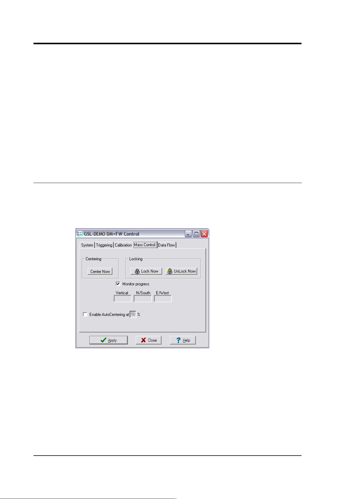
Scream! 4.5

the rate to 4 (Hz). In this manner, you can select frequencies ranging from 0.1 to 10 Hz (10 to 0.1 s periods).

You can specify step calibration by selecting the Square wave button. The square wave consists of a positive step at the start of the next minute of the digitiser’s internal clock, followed by a negative step after a specified number of minutes. After a further delay of the same number of minutes, the calibration signal is disconnected. The default is two minutes. The Period and Frequency are ignored.

The Broadband Noise calibration signal consists of a constant stream of white noise, which lasts for the specified number of minutes. The Period and Frequency are ignored.

8.4 Mass Control

Many Güralp instruments respond to control signals to centre, unlock, and lock the sensor masses. These signals are generated by the digitiser. You can tell the digitiser to send a signal using the Centre Now, Lock Now and UnLock Now buttons on the Mass Control tab.

If you tick the Monitor progress check-box, the window will remain open during the process, and the mass positions will be displayed in the Vertical, N/South and E/West boxes. If you leave Monitor progress clear, the window will close while the operation takes place. You can still monitor the mass positions by selecting the appropriate streams and opening a WaveView window for them.

Depending on which Sensor Type you have chosen in the System tab (see above), not all the control signals will be available. For example, CMG-3ESP sensors can be centred from Scream!, but must be locked

92 Issue K

User guide

and unlocked manually, whilst a CMG-3T has remote lock and unlock commands.

CMG-40T, CMG-6T seismometers and CMG-5T strong-motion instruments do not need locking or unlocking. If you have set the Sensor Type to one of these sensors, the Mass Control tab will not be available.

8.5 Data flow

The digitiser operates in one of several transmission modes. These modes relate to how the unit uses its Flash memory:

• as a simple data store, from which you can request data (FILING

and DUAL modes);

• as a buffer holding unacknowledged blocks, which are

transmitted in preference to real-time data (FIFO mode);

• as a buffer holding unacknowledged blocks, which are

transmitted whenever the transmission is free and no real-time data blocks are ready (ADAPTIVE mode);

• not at all (DIRECT mode).

Separate from these modes are buffering modes, which tell the unit what to do when its Flash memory becomes full: It can either

• carry on, overwriting the oldest data held, or

• stop writing and switch the digitiser into DIRECT mode.

You can switch between transmission modes in Scream! by right-clicking on the digitiser and clicking on Control…, then navigating to the Data Flow pane:

January 2014 93

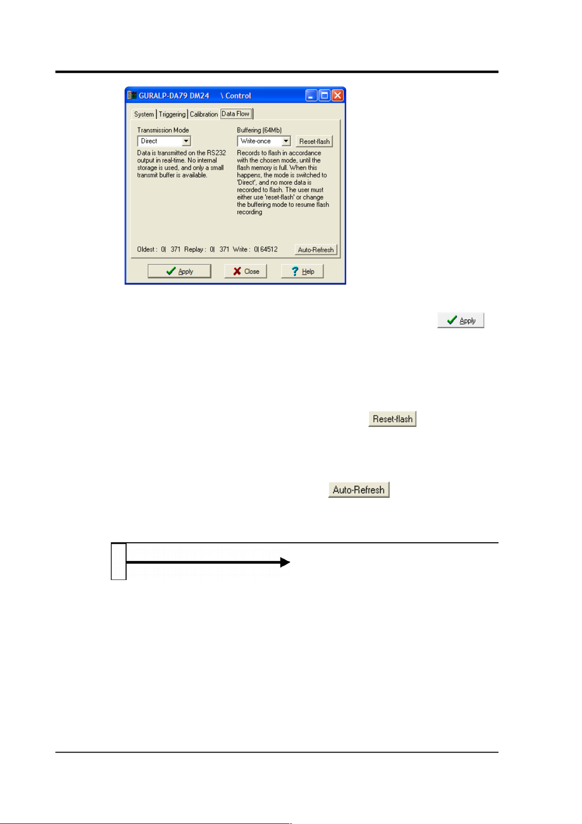
Scream! 4.5

To choose a transmission or buffering mode, choose options from the Transmission Mode or Buffering drop-down menus, and click .

An explanation of the chosen mode is displayed beneath each menu. The following sections also explain the transmission modes available.

The Buffering legend also displays the amount of Flash memory present in your digitiser.

To clear the Flash memory of the digitiser, click . You will be asked for confirmation before the memory is cleared.

At the bottom of the tab is a line describing the current state of the digitiser's memory pointers. You can use this line to check that data

are being written into memory. Click to make the line update automatically.

8.5.1 DIRECT

Instructs the digitiser not to use Flash memory for storage. Instead, all data are transmitted directly to clients. An instrument in DIRECT mode still honours the GCF Block Recovery Protocol: a temporary RAM buffer always holds the last 256 blocks generated, and if a client fails to receive a block it can request its retransmission.

If you expect breaks in communication between the instrument and its client to last more than 256 blocks, or if you want the instrument to handle breaks in transmission (rather than relying on the client to request missed blocks), you should use

94 Issue K

User guide

• ADAPTIVE mode, if you want data to stay as near to real time as

possible (but do not mind if blocks are received out of order) or

• FIFO mode, if you need blocks to be received in strict order (but

do not mind if the instrument takes a while to catch up to real time).

8.5.2 FILING

Instructs the digitiser not to transmit blocks to clients automatically, but to store all digitized data in the Flash memory. If you have chosen the RECYCLE buffering mode (see below), the memory is used in circular fashion, i.e. if it becomes full, incoming blocks begin overwriting the oldest in memory. If the WRITE-ONCE mode is active, the instrument will switch to DIRECT mode (see above) when the memory becomes full.

Heartbeat messages

When in FILING mode, an instrument transmits “heartbeat” messages over its data port. These short messages take the place of data blocks, and ensure that programs such as Scream! know that an instrument is present.

If your digitiser is in FILING mode, Scream! will displays a slider at the bottom of the tab. Moving this slider changes the interval between heartbeat blocks.

You can tell Scream! to download new data automatically whenever it receives a heartbeat message from an instrument in FILING mode. This is useful, for example, in autonomous installations connected by intermittent modem links. To enable this feature:

January 2014 95

Scream! 4.5

1. Choose File Setup… → from Scream!'s main menu, and navigate to the Recording pane.

2. Tick Auto-download on heartbeat.

3. Click

Using FILING mode with Auto-download on heartbeat ensures that Scream! receives all new data whenever it can, regardless of the configuration of any devices between Scream! and the instrument.

8.5.3 DUPLICATE

Instructs the DM24 to transmit streams directly to clients (as for

DIRECT mode) but also to store all data into Flash storage (as for FILING mode).

If a client fails to acknowledge a block, the digitiser does not attempt to retransmit it.

Heartbeat messages are not sent in DUPLICATE mode.

96 Issue K

User guide

8.5.4 DUAL

Instructs the digitiser to transmit any continuous streams directly to clients as for DIRECT mode, but to store triggered data into Flash storage as for FILING mode.

If you choose DUAL mode but do not select any continuous streams for output, the instrument will send heartbeat messages as for FILING mode. Scream! can pick these up and download new data as necessary.

8.5.5 FIFO (First In First Out)

Instructs the digitiser to begin writing blocks to Flash memory as for FILING mode, but also to transmit data to clients. Data are transmitted in strict order, oldest first; the digitiser will only transmit the next block when it receives an explicit acknowledgement of the previous block.

If the communications link is only marginally faster than the data rate, it will take some time to catch up with the real-time data after an outage. If you want data to be transmitted in real-time where possible, but are worried about possible breaks in communication, you should use ADAPTIVE mode instead.

FIFO mode will consider a data block successfully transmitted once it has received an acknowledgement from the next device in the chain. If there are several devices between you and the instrument, you will need to set up the transmission mode for each device (if applicable) to ensure that data flow works the way you expect.

Like all the transmission modes, FIFO mode does not delete data once it has been transmitted. You can still request anything in the Flash memory using Scream! or over the command line. The only way data

January 2014 97

Scream! 4.5

can be deleted is if it is overwritten (in the RECYCLE buffering mode, see below) or if you delete it manually.

8.5.6 ADAPTIVE

Instructs the digitiser to transmit current blocks to clients if possible, but to store all unacknowledged blocks in the Flash memory and re-send them, oldest first, when time allows. ADAPTIVE mode is best suited for “real-time” installations where the link between digitiser and client is intermittent or difficult of access.

If the communications link is only marginally faster than the data rate, it will usually be busy transmitting real-time data. Thus, it may take a while for the instrument to work through the missed blocks. In this case, and if your client supports it, you may prefer to use the Block Recovery Protocol to request missed blocks where possible.

Some software packages (most commonly Earthworm) cannot handle blocks being received out of time order. If you are using such a package, ADAPTIVE mode will not work, and may crash the software.

98 Issue K

User guide

8.5.7 Transmission mode summary

Transmission Mode:

DIRECT

FILING

DUPLICATE

DUAL

FIFO

ADAPTIVE

Transmit continuous data: ✔ ✘ ✔ ✔ ✔ ✔

Store continuous data: ✘ ✔ ✔ ✘ ✔ ✘

Transmit trigger data: ✔ ✘ ✔ ✘ ✔ ✔

Store trigger data: ✘ ✔ ✔ ✔ ✔ ✘

Heartbeat messages:

✘ ✔ ✘ ?

✘ ✘

Strict time order: ✔2n/a ✔2✔

✔ ✘

Retransmit unacknowledged blocks: ✔4n/a ✘ ✘ ✔5✔

Notes:

1. Heartbeat messages will only be sent if no continuous streams are enabled

2. The receiver can request a “rewind” if blocks are not received correctly but retransmission resumes in strict time order

3. Real-time data are prioritised over missed blocks

4. Up to 256 blocks can be buffered to satisfy rewind requests

5. The whole of flash memory is used as a retransmission buffer

8.6 Buffer Memory Usage

8.6.1 RE-USE / RECYCLE

Instructs the digitiser to carry on using the current transmission mode when the Flash memory becomes full, overwriting the oldest data held. This buffering mode is called RECYCLE in Scream! and on the EAM.

For example, in DUAL mode with RECYCLE buffering, the latest continuous data will be transmitted to you as normal, and the latest triggered data may be retrieved from the Flash memory using Scream! or the command line. However, if you do not download data regularly from the Flash memory, you may lose older blocks. This mode thus lets you prioritise the most recent data held by the instrument.

January 2014 99

Scream! 4.5

8.6.2 WRITE-ONCE

Instructs the digitiser to stop writing data to the Flash memory when it is full, and to switch to DIRECT mode automatically.

For example, in FIFO mode with WRITE-ONCE buffering, the station will transmit data to you continuously, but also save it in the Flash memory until it is full. Once full, the instrument will switch to DIRECT mode and continue transmitting, though no further data will be saved. This mode thus lets you prioritise the earliest data held by the instrument.

100 Issue K

Guralp Systems Scream User Manual

Specifications and Main Features

Frequently Asked Questions

User Manual