Guralp Systems ART User Manual

ART 3.0

Seismic Analysis and Research
Tool

User guide

Part No. MAN-SWA-0003

Designed and manufactured by
Güralp Systems Limited
3 Midas House, Calleva Park
Aldermaston RG7 8EA
England

Proprietary Notice: The information in this
manual is proprietary to Güralp Systems Limited
and may not be copied or distributed outside the
approved recipient's organisation without the
approval of Güralp Systems Limited. Güralp
Systems Limited shall not be liable for technical
or editorial errors or omissions made herein, nor
for incidental or consequential damages resulting
from the furnishing, performance, or usage of this
material.

Issue C 2009-05-01

ART

Table of Contents

1 Introduction...........................................................................4

2 Getting Started.......................................................................7

2.1 Installing ART.....................................................................................7

2.2 Setting up sensor information............................................................7

2.2.1 Examples......................................................................10

2.3 Starting ART.....................................................................................11

2.3.1 Start from the ART icon................................................11

2.3.2 Starting from SCREAM..................................................11

3 Using ART.............................................................................13

3.1 Importing data from Scream!...........................................................13

3.2 The main ART window......................................................................13

3.2.1 Import data .................................................................14

3.2.2 Options.........................................................................15

3.2.3 Interactive selection of filter parameters.....................19

3.2.4 Add/edit metadata.......................................................20

3.2.5 Filter time-histories......................................................23

3.2.6 Export data...................................................................23

3.2.7 Clear time-histories......................................................26

3.2.8 Event Manager.............................................................27

3.2.9 ‘Unfiltered?’ check box.................................................27

3.2.10 Central list box.............................................................27

3.2.11 Strong-motion parameters...........................................28

3.2.12 View time-histories.......................................................34

3.2.13 View time-histories on map..........................................36

3.2.14 Particle motions...........................................................37

3.2.15 Husid (Arias intensity) plot...........................................39

3.2.16 Energy density plot......................................................40

3.2.17 Fourier amplitude spectrum.........................................42

3.2.18 Elastic response spectra..............................................45

3.2.19 Elastic input energy spectra.........................................47

3.2.20 Drift spectra.................................................................49

3.2.21 Comparisons................................................................50

4 References...........................................................................54

2 Issue C

User guide

5 Software Change History.......................................................60

5.1 Changes from ART 2.........................................................................60

5.2 Changes from ART 1.........................................................................61

6 Revision history....................................................................63

May 2009 3

ART

1 Introduction

ART 3.0, Güralp Systems' Strong-Motion Analysis and Research
Tool is a windows program which allows users of seismometers
(accelerometers or velocimeters) produced by Güralp Systems
Ltd, to process and analyze their recorded data for engineering
seismology and earthquake engineering purposes. The time­histories can be exported in a number of different strong­motion record formats that are currently in use today.

ART3.0 is a major update of the second version of ART
(ART2.0), which was released in 2006. A number of
improvements were made following requests received from
users, which are listed in section 5.1, page 60.

ART 3.0 is supplied in the standard distribution of Scream!
versions 4.5 and later. It is also compatible with older versions
of Scream!.

ART works closely with Scream! to make analysing seismic data
easy. Scream!'s visualization and filtering capabilities allow you
to view time series and quickly identify events. Strong-motion
records can then be directly imported into ART from Scream!
by selecting the appropriate portion of the record in Scream! ­this will automatically start ART. Previously recorded data in
Güralp Compressed Format (GCF) can be read in from pre­recorded files and analyzed. In addition, data can be imported
into ART via a modem.

Currently the following functions, which are important for
engineering seismologists and earthquake engineers, are
supported (in addition most of these functions allow selection
of multiple time-histories so a comparison between records is
possible).

• plotting uncorrected acceleration, velocity and

displacement against relative or absolute time;

• automatic correcting of recorded time-history for

instrument response to obtain ground acceleration;

• filtering of acceleration time-history using user-defined

filters;

• plotting corrected acceleration, velocity and

displacement against relative or absolute time;

4 Issue C

User guide

• calculation and plotting of Fourier amplitude spectra of

time-histories and of pre-event portions of records
including the signal-to-noise ratios;

• calculation and plotting of Arias intensities against time;

• calculation and plotting of energy densities against time;

• calculation and plotting, both on standard and tripartite

graphs, of linear elastic response spectra;

• calculation and plotting of linear elastic absolute and

relative input energy spectra;

• calculation and plotting of drift spectra for a cantilever

shear-beam for different material types;

• calculation of peak ground acceleration (PGA), peak

ground velocity (PGV) and peak ground displacement
(PGD);

• calculation of PGV/PGA;

• calculation of A95 parameter;

• calculation of sustained maximum acceleration and

velocity;

• calculation of JMA instrumental intensities;

• calculation of response spectrum intensities using user-

defined limits;

• calculation of acceleration spectrum intensities using

user-defined limits;

• calculation of RMS acceleration, velocity and

displacement;

• calculation of cumulative absolute velocities using user-

defined minimum acceleration thresholds;

• calculation of absolute and relative bracketed, significant

and uniform strong-motion durations using user-defined
limits;

May 2009 5

ART

• calculation of number of absolute and effective cycles of

acceleration using peak counting - including or excluding
non-zero crossings and rainflow counting techniques;

• calculation of mean, predominant spectral, smoothed

spectral predominant and average spectral periods;

• plotting particle motions both in two and three

dimensions;

• basic database functionality to allow earthquake and

station metadata to be added, used and exported;

• comparison of observed elastic response spectra to

predicted spectra from various ground-motion prediction
equations and seismic design codes;

• plotting of acceleration, velocity and displacement time-

histories on map;

• exporting the uncorrected and corrected spectra in these

commonly used strong-motion record formats:

• Columns;

• CSMIP as used by the California Strong-Motion

Instrumentation Program;

• ISESD as used by the Internet Site for European

Strong-Motion Data;

• K-Net as used by Kyoshin Net;

• PEER as used by Pacific Earthquake Engineering

Research Center;

• SMC as used by the US Geological Survey;

• SAC as used by Seismic Analysis Code;

• Microsoft Excel .xls;

• Matlab .mat.

6 Issue C

User guide

2 Getting Started

The material in this chapter covers the installation,
configuration and invocation of ART 3.0.

2.1 Installing ART

ART is included in the standard Scream! distribution for
Windows, which is available for free download.

ART uses the Matlab runtime library for its mathematical
routines. This is supplied as part of the installer and may be
freely distributed.

To download Scream!, send an e-mail to [e-mail],
including information about your institution and the type(s) of
equipment you are using.

To install the package, double-click on its icon and follow the
instructions in the installer. Choose the Typical installation
option to ensure that ART and its supporting libraries are all
installed.

2.2 Setting up sensor information

Before it can analyse data from your instruments, ART needs to
know detailed calibration information for each one.

Note:

If you start ART from within Scream! (as in section 2.3.2
on page 11) without setting up the relevant sensor information,
you will receive an error message saying:

A VPC= entry for {SYSTEM_ID-SERIAL} was not found in
calvals.txt

and you should follow the procedure in this section before re­trying.

The calibration information must be provided in a file called
calvals.txt, which should be kept in the ART/Scream!
program directory. You can create and edit this file from inside
Scream! by right-clicking on the digitizer's icon in the main

window and selecting Calvals....

The file is divided into sections, each beginning with a title in
square brackets. The title gives the System ID and serial

May 2009 7

ART

number (as given by the first four characters of the Stream ID)
for the digitizer which produces the data stream.

For example: to add calibration information for a digitizer with
System ID GURALP outputting streams DEMOZ2, DEMON2,
DEMOE2, etc., you would add a section beginning with the line

[GURALP-DEMO]

If you move an instrument from one digitizer to another, you
will need to update the calvals.txt file to reflect the change.

• To set the serial number of the instrument, include the

line

Serial-Nos=serial-number

• Scream! cannot tell what instrument is connected to the

digitizer. This line is provided to help you remember
which set of calibration values you have used, and to
provide a title for calibration graphs. If you attach a
different instrument to the same digitizer, you will need
to enter new calibration values to reflect the new
instrument.

• To set the sensitivity of the digitizer, include the line

VPC=sensitivity

VPC stands for voltage per count, measured in units of
μV/count. This is sometimes given as μV/Bit on the digitizer
calibration sheet.

• To set the sensitivity of the calibration channel, include

the line

CALVPC=sensitivity

as for the other digitizer channels.

• To set the value of the calibration resistor, include the

line

CALRES=resistance

Güralp Systems digitizers normally use a 51 kΩ resistor
(CALRES=51000).

• To set the sensor type, include the line

8 Issue C

User guide

TYPE=model-number

e.g. 3T, 5T, etc..

• To set the response of the sensor, include the line

RESPONSE=response-type unit

The values you can use are given in the table below.

Sensor

Sensor type code
(response-type)

Units
(V/A)

CMG-5T or 5TD,
DC – 100 Hz response

CMG-5_100HZ

A

CMG-40T-1 or 6T-1,
1 s – 100 Hz response

CMG-40_1S_100HZ

V

CMG-40T-1 or 6T-1,
2 s – 100 Hz response

CMG-40_2S_100HZ

V

CMG-40T-1 or 6T-1,
10 s – 100 Hz response

CMG-40_10S_100HZ

V

CMG-40, 20 s – 50 Hz response

CMG-40_20S_50HZ

V

CMG-40, 30 s – 50 Hz response

CMG-40_30S_50HZ

V

CMG-3T or 3ESP,
30 s – 50 Hz response

CMG-3_30S_50HZ

V

CMG-40, 60 s – 50 Hz response

CMG-40_60S_50HZ

V

CMG-3T or 3ESP,
60 s – 50 Hz response

CMG-3_60S_50HZ

V

CMG-3T or 3ESP,
100 s – 50 Hz response

CMG-3_100S_50HZ

V

CMG-3T or 3ESP,
120 s – 50 Hz response

CMG-3_120S_50HZ

V

CMG-3T, 360 s – 50 Hz response

CMG-3_360S_50HZ

V

CMG-3TB or 3V / 3ESP borehole,
30 s – 50 Hz response

CMG-3B_30S_50HZ

V

CMG-3TB or 3V / 3ESP borehole,
100 s – 50 Hz response

CMG-3B_100S_50HZ

V

CMG-3TB or 3V / 3ESP borehole,
120 s – 50 Hz response

CMG-3B_120S_50HZ

V

CMG-3TB or 3V / 3ESP borehole,
360 s – 50 Hz response

CMG-3B_360S_50HZ

V

May 2009 9

ART

Sensor

Sensor type code
(response-type)

Units
(V/A)

CMG-3TB or 3V / 3ESP borehole,
360 s – 50 Hz response

CMG-3B_360S_100HZ

V

Some English descriptions are also accepted, e.g.
“120s velocity”, “100Hz acceleration”.

• To set the sensitivities (or gains) of the sensor

components, include the line

G=vertical-sens,N/S-sens,E/W-sens

These values are given on the sensor calibration sheet. For
velocity sensors, they are given in units of V m–1 s (V/m/s).
The gain of an accelerometer is expressed in V m-1 s2 (V/m/
s2). Because Güralp Systems sensors and digitizers use
differential inputs and outputs, the sensitivity is quoted as
2 × (single-ended sensitivity) on the calibration sheet.

• To set the coil constants of the sensor components,

include the line

COILCONST=ZCC,NCC,ECC

Where ZCC is the vertical coil constant, NCC is the
North/South coil constant and ECC is the East/West cost
constant. These values are given on the sensor calibration
sheet.

• To set the local acceleration due to gravity, include the

line

GRAVITY=acceleration

You should give this value in m s–2, if you know it. If you
miss out this line, Scream! will use a standard average
g value of 9.80665 m s–2.

2.2.1 Examples

The calibration information for a CMG-3T weak-motion velocity
sensor might look like the following:

[GURALP-CMG3]
Serial-Nos=T3X99
VPC=3.153,3.147,3.159
G=1010,1007,1002

10 Issue C

User guide

COILCONST=0.02575,0.01778,0.01774
CALVPC=3.161
CALRES=51000
TYPE=CMG-3T
RESPONSE=CMG-3_30S_50HZ V
GRAVITY=9.80122

CMG-5TD accelerometers use 1 Ω calibration resistors, and
their coil constant is set to unity. Older CMG-5TD instruments,
based on Mk2 digitizer hardware, do not have calibration input
facilities, and thus the CALVPC entry is omitted. For example:

[GURALP-CMG5]
Serial-Nos=T5585
VPC=2.013,2.028,2.036
G=0.256,0.255,0.255
COILCONST=1,1,1
CALRES=1
TYPE=CMG-5T
RESPONSE=CMG-5_100HZ A
GRAVITY=9.81089

2.3 Starting ART

ART can be started in two ways, either from SCREAM or by
double clicking on the ART icon.

2.3.1 Start from the ART icon

Double-clicking on the ART icon will start the application and
cause the main ART window to open.

Clicking on the ‘Import data’ button at the top of the left-hand
column of the main ART window opens up a file selection
window from which a GCF time-history can be selected to
import and analyze.

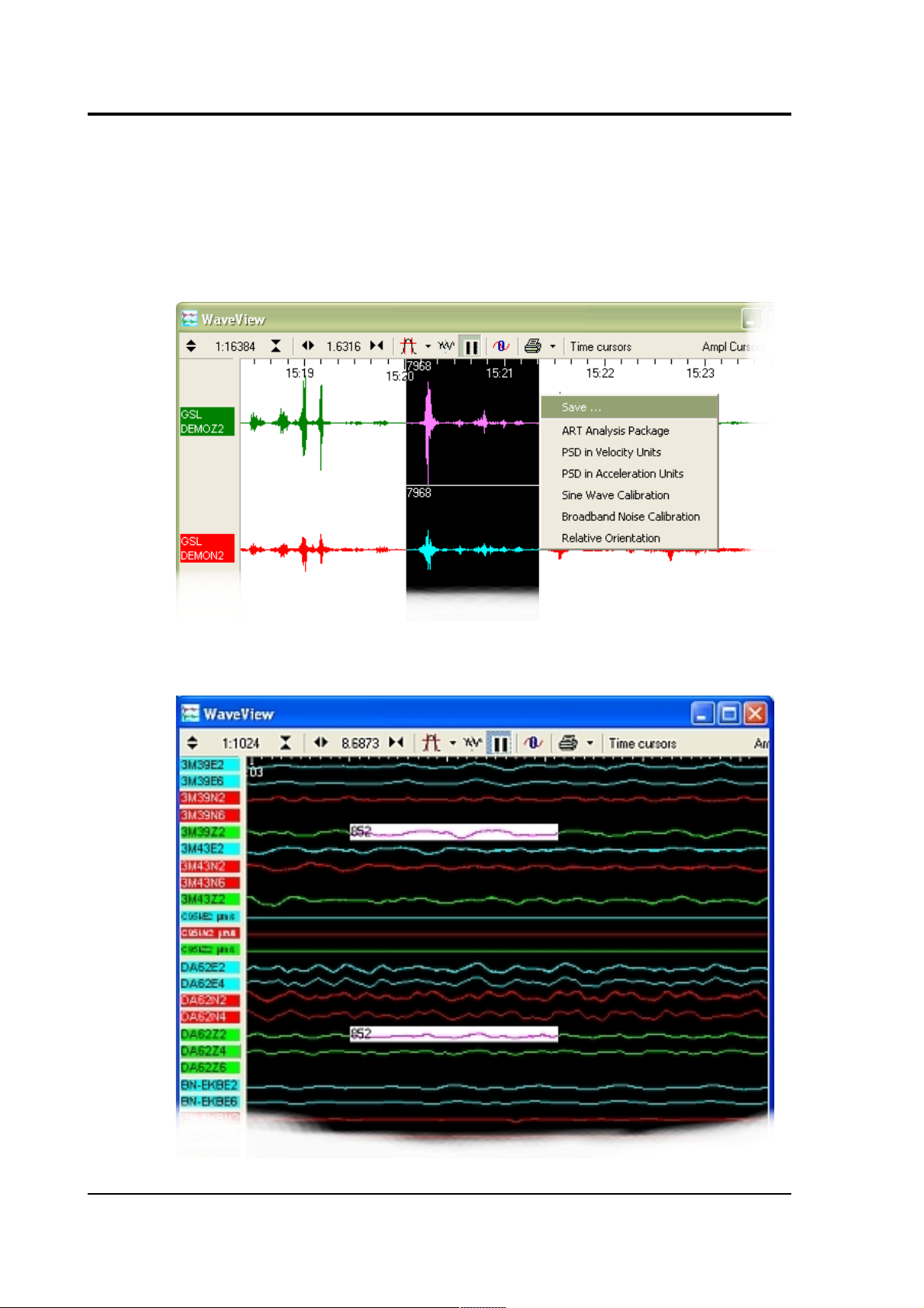
2.3.2 Starting from SCREAM

Within Scream!, open a WaveView window displaying the event
you are interested in. Click on the Pause icon to stop the

traces moving then, using the mouse, select the parts of the
time-histories that you want to analyze while holding down
either the Ctrl or Shift keys.

If you use the Ctrl key, the

first

and

last

streams in the selected
area will be analyzed. This is useful for picking two streams
from many for comparison. If you use the Shift key, a
contiguous set of streams are selected.

May 2009 11

ART

When the Ctrl or Shift key is released, a pop-up menu will
appear (after a short delay) asking which add-on program you
want to run. Select ART and the main ART window will open
with the selected time-histories automatically loaded.

The picture below shows a Scream! WaveView window with two
streams selected (using the Shift key).

The second illustration shows the selection of two non-adjacent
streams for comparison, using the Ctrl key

12 Issue C

User guide

3 Using ART

The following sections discuss the features currently
implemented in ART and how to use them.

When a time-history is loaded into ART, either via SCREAM, via
the Import Data button (see below) or via the Event Manager, a
correction for instrument response and, if required, a
conversion to acceleration is automatically performed. Low­pass filtering with a transition band given in ‘Options’ window
(see below) is also undertaken, The algorithm used to remove
the instrument response is the same as that used in BAP v1.0
(Converse & Brady, 1992) but the transfer function used to
correct the time-history is derived from the poles and zeros of
the originating instrument (e.g. a CMG-5T).

3.1 Importing data from Scream!

The most common and convenient way to get data into ART is
to import it directly from a WaveView window within Scream!.
This is fully described in section 2.3.2 on page 11. It is also
straightforward to import GCF files without running scream.
This is described in section 3.2.1 on page 14.

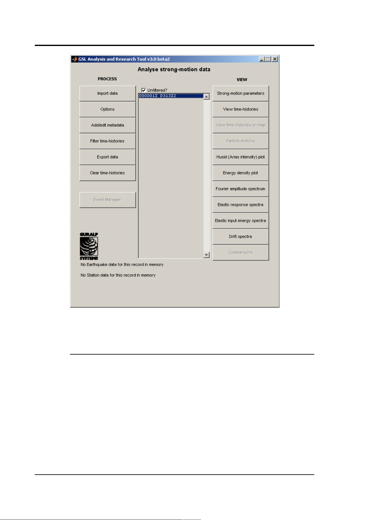
3.2 The main ART window

The main ART window has:

• two columns of buttons (PROCESS and VIEW) for

analyzing and processing the selected time-histories;

• a list box in the middle for choosing which time-history is

being processed and analyzed; and

• a text box at the bottom for displaying the metadata on

the earthquake and station associated with the selected
time-history (this information is only displayed if a single
time-history is selected).

The full window is shown overleaf.

The following sections discuss the available functions starting
with the left-hand column of buttons (PROCESS).

May 2009 13

ART

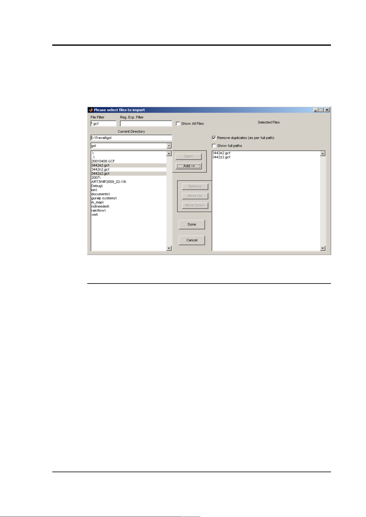
3.2.1 Import data

Clicking on the ‘Import data’ button at the top of the left-hand
column opens up a file selection window from which the GCF
time-history to import can be selected (see below).

Many time-histories can be loaded into ART using this file
selection window and, in addition, the window can be opened
as many times as required to load in all the data required.
Once the required time-histories have been located, double
clicking on the filenames (multiple records can be selected by
holding down the Shift or Ctrl keys) or clicking on the filenames
and clicking ‘Add’ will add them to the list of files to import (in
the right-hand list box). To import the data listed in the right-

14 Issue C

User guide

hand list box) click on ‘Done’ and their names will be added to
the list given in the central box. As stated above, the data is
automatically corrected for instrument response and converted
to acceleration, if required.

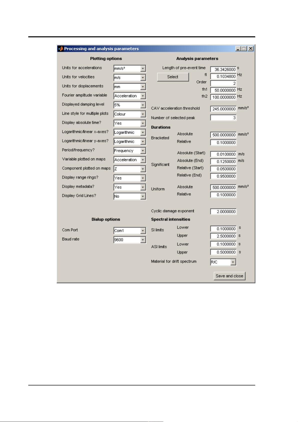
3.2.2 Options

Clicking on the ‘Options’ button opens a window (see below)
displaying the options that are currently used for display of
acceleration, velocity and displacement parameters,
appearance of some windows, filtering and for the calculation
of the strong-motion parameters. The parameters given in this
window can be altered either by clicking in the white box next
to the name of the parameter and editing its contents or by
using the pull-down menus.

May 2009 15

ART

The parameters that can be changed in this window are:

1. units used for display of accelerations (‘Units for
accelerations’) (g, m/s2, cm/s2 or mm/s2);

2. units used for display of velocities (‘Units for velocities’)

(m/s, cm/s or mm/s);

3. units used for display of displacements (‘Units for

accelerations’) (m, cm or mm);

4. variable used for calculation of Fourier amplitude spectra

(acceleration, velocity or displacement);

5. damping level used in figures comparing the response

16 Issue C

User guide

spectra of two or more records (0, 2, 5, 10 or 20%);

6. line styles used for figures comparing the derived strong­motion parameters of two or more records (monochrome or
colour);

7. whether absolute time is reported on the graphs showing
acceleration, velocity and displacement time-histories (yes
or no);

8. whether to use logarithmic or linear x-axes for graphs
(logarithmic or linear);

9. whether to use logarithmic or linear y-axes for graphs
(logarithmic or linear);

10. whether to use period or frequency for graphs and
parameter display (period or frequency);

11. which variable to plot on maps displaying time-histories
(acceleration, velocity or displacement);

12. which component to plot on maps displaying time-histories
(Z, N or E);

13. whether to display range rings on maps displaying time­histories (yes or no);

14. whether to display metadata in title of figures (yes or no);

15. whether to display grid lines on figures (yes or no):

16. what COM port to use for dialling stations (COM1 is the only
option currently supported);

17. what baud rate to use for dialling stations (2400, 4800,
9600, 19200, 38400, 57600 or 115200);

18. length of pre-event time to use for calculating noise
estimate (‘Length of pre-event time’) in seconds (if this is
set to zero then a noise spectrum is not calculated). This can
be selected interactively by clicking on the ‘Select’ button,
see below;

19. corner frequency (‘fl’) in Hz of the bi-directional filter used
for high pass filtering time-histories (usually this is about

0.05Hz for records from CMG-5Ts and it cannot be less than
0Hz). This can be selected interactively by clicking on the
‘Select’ button, see below;

20. order (‘Order’) of the Butterworth filter used for high pass
filtering time-histories (the default value for the order is 2, a
higher order filter has a steeper transition band but requires
more zero padding and the filtering takes a longer time).
This can be selected interactively by clicking on the ‘Select’
button, see below;

21. frequency where cosine taper of low pass filter starts (‘fh1’)
in Hz (usually this should be about 50Hz for records from
CMG-5s);

22. frequency where cosine taper of low pass filter ends (‘fh2’)
in Hz (usually this should be about 100Hz for records from
CMG-5s);

May 2009 17

ART

23. acceleration threshold to use within the computation of
cumulative absolute velocity (CAV) (this must be positive). A
commonly-used threshold is 0.025g [0.245m/s2];

24. the number of the peak to select for computation of the
sustained maximum acceleration and velocity (this must be
a positive integer). A commonly-used value is 3, denoting
the third peak;

25. acceleration used as the limit acceleration in the calculation
of bracketed absolute duration (‘Bracketed Absolute’) in the
selected units of acceleration. A commonly used limit
acceleration is 0.05g [0.49m/s2];

26. proportion of peak ground acceleration used as the limit
acceleration in the calculation of bracketed relative duration
(‘Bracketed Relative’). This must be between 0 and 1;

27. value of Arias intensity used as the lower threshold in the
calculation of significant absolute (effective) duration in the
selected units of velocity (see Bommer & Martinez-Pereira,

1999) (‘Significant Absolute (Start)’). A commonly used
lower limit is 0.01m/s;

28. value of Arias intensity used as the upper threshold in the
calculation of significant absolute (effective) duration in the
selected units of velocity (see Bommer & Martinez-Pereira,

1999) (‘Significant Absolute (End)’). A commonly used lower
limit is 0.125m/s;

29. proportion of Arias intensity used as the lower limit in the
calculation of significant relative duration (‘Significant
Relative (Start)’). This value must be between 0 and 1 - a
commonly used lower limit is 0.05;

30. proportion of Arias intensity used as the upper limit in the
calculation of significant relative duration (‘Significant
Relative (End)’). This value must be between 0 and 1 - a
commonly used upper limit is 0.95;

31. acceleration used as the limit acceleration in the calculation
of uniform absolute duration (‘Uniform Absolute’) in the
selected units of acceleration. A commonly used limit
acceleration is 0.05g [0.49m/s2];

32. proportion of peak ground acceleration used as the limit
acceleration in the calculation of uniform relative duration
(‘Uniform Relative’). This value must be between 0 and 1;

33. cyclic damage exponent to use for the computation of the
effective number of cycles. A commonly used value is 2;

34. period used as lower limit in calculation of spectral intensity
(‘SI limits Lower’). A commonly used lower limit is 0.1s;

35. period used as upper limit in calculation of spectral intensity
(‘SI limits Upper’). A commonly used upper limit is 2.5s;

36. period used as lower limit in calculation of acceleration
spectral intensity (‘ASI limits Lower’). A commonly used

18 Issue C

User guide

lower limit is 0.1s;

37. period used as upper limit in calculation of acceleration

spectral intensity (‘ASI limits Upper’). A commonly used
upper limit is 0.5s.

38. the material to assume for the computation of the drift

spectra (steel, R/C or other)

Clicking on the ‘Save’ button saves the chosen parameters to a
file called art_default.dat which is loaded each time ART is
used. The parameters are not automatically saved when the
window is close using the close icon; however, they are used
for the rest of the session.

3.2.3 Interactive selection of filter parameters

The

Order

and corner frequency

fl

of the Butterworth filter, as

well as the

Length of pre-event time

, can be set interactively.

1. Select a single stream in the centre panel of the main
window. Click Options.

2. In the

Options

window, beneath the legend

Length of

pre-event time

, click the Select button. A window will

pop up displaying the stream you have selected.

3. The top two graphs show the acceleration and
displacement time histories for the selected stream, with
the current low-pass filter applied.

4. The red line shows the current

Length of pre-event time

setting. Data before the line is used to calculate spectra
of ambient ground motion; data after it is treated as part
of the event.

Click in either graph to move the line. The spectra below
are updated automatically.

5. The plot at bottom left shows the Fourier amplitude
spectrum of ambient ground motion (in blue) and of the
event (in black), using the current filter settings.

The plot at bottom right shows the ratio between the two
spectra (

i.e.

the signal-to-noise ratio). The horizontal red
lines represent signal-to-noise ratios of 2:1 and 1:2; the
blue lines represent ratios of 3:1 and 1:3.

May 2009 19

ART

The vertical red line in each graph shows the corner
frequency currently being used for the low-pass filter.
Click in the graph to move it. The time histories above
are updated automatically.

6. To change the order of the applied filter, choose an
option from the

Order

drop-down menu. Filters of first to

sixth order can be applied.

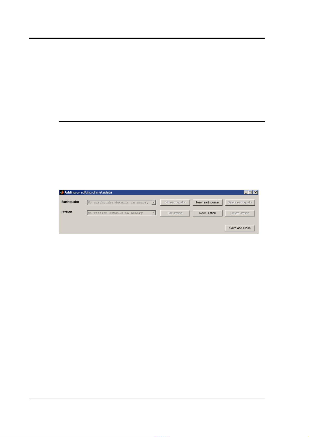
3.2.4 Add/edit metadata

Clicking on this button (this button is only enabled when a
single time-history is selected in the central list box) will open a
window that enables the user to enter, edit and delete basic
metadata on the earthquake and station concerning the record
selected. Metadata that has already been entered in a previous
use of ART is loaded into memory when ART is launched. In
addition, the meta-data is automatically saved to a file when
this metadata window is closed.

Clicking on the ‘New earthquake’ button (or the ‘Edit
earthquake’ button once a record is assigned to an earthquake)
will open up a window where basic meta-data on the
earthquake can be added (or edited).

Clicking on the ‘New station’ button (or the ‘Edit station’ button
once a record is assigned to a station) will open up a window
where basic metadata on the station can be added (or edited).

Clicking on the ‘Save and Close’ button saves the metadata
and closes the window.

When metadata on earthquakes is in memory the selected
time-history can be associated (or re-associated) to an event
by using the Earthquake combo box. Similarly, when metadata
on stations is in memory the selected time-history can be
associated (or re-associated) to a station by using the Station
combo box.

20 Issue C

User guide

Adding or editing earthquake information

The earthquake date and time fields are automatically filled by
ART by using the time at which the time-history begins.
However, this information can be modified by the user by
clicking in the white boxes and modifying the values. Similarly
the user can modify the other event information reported in
this window by clicking in the white boxes and modifying the
text or by using the pull-down menus.

Once the user has entered the information on the event
clicking on the OK button will store the entered metadata in
memory and close the window. If the Cancel button is selected
the window is closed without storing the entered metadata.

May 2009 21

ART

Deleting earthquake information

If the user wishes to delete the entire set of information
concerning the earthquake associated with a time-history then
they should click on the ‘Delete earthquake’ button in the
Adding and editing metadata window. This will clear the
metadata from memory and also will remove the link between
the record and the event.

Adding or editing station information

The user can modify the information by clicking in the white
boxes and changing the text or by using the pull-down menus.

Once the user has entered the information on the station
clicking on the OK button will store the entered metadata in
memory and close the window. If the Cancel button is selected
the window is closed without storing the entered metadata.

Deleting station information

If the user wishes to delete the entire set of information
concerning the station associated with a time-history then they
should click on the ‘Delete station’ button in the ‘Adding and
editing metadata’ window. This will clear the metadata from
memory and also will remove the link between the record and
the station.

22 Issue C

User guide

3.2.5 Filter time-histories

Clicking on this button will filter the currently selected time­histories using a high pass bi-directional Butterworth filter with
corner frequency and order given in ‘Options’ window (‘fl’ and
‘order’ are the corner frequency and order used for the
filtering). The algorithm used to do the filtering is the same as
that used in BAP v1.0 (Converse & Brady, 1992), which zero­pads the time-history. Note that the time to accomplish the
filtering has been significantly reduced in ART3.0 in comparison
to earlier versions.

3.2.6 Export data

Clicking on this button opens
up a window that enables the
user to export uncorrected
acceleration time-histories,
corrected acceleration, velocity
and displacement time­histories, Fourier amplitude
spectra, elastic response
spectra, input energy spectra
and drift spectra in a variety of
different formats. A new
window is opened with six
buttons.

Clicking on the top button will
export uncorrected
acceleration time-histories.
Clicking on the next button
down will export the corrected
acceleration, velocity and

displacement time-histories (if
the time-histories selected have not been filtered then the
uncorrected time-histories will be exported). Clicking on the
next button will export the Fourier amplitude spectra (the
spectra will be calculated). Clicking on the next button down
will export the calculated elastic response spectra (the spectra
will be calculated). Clicking on the next button will export the
input energy spectra (the spectra will be calculated) and
clicking on the lowest button will export the calculated drift
spectra.

May 2009 23

ART

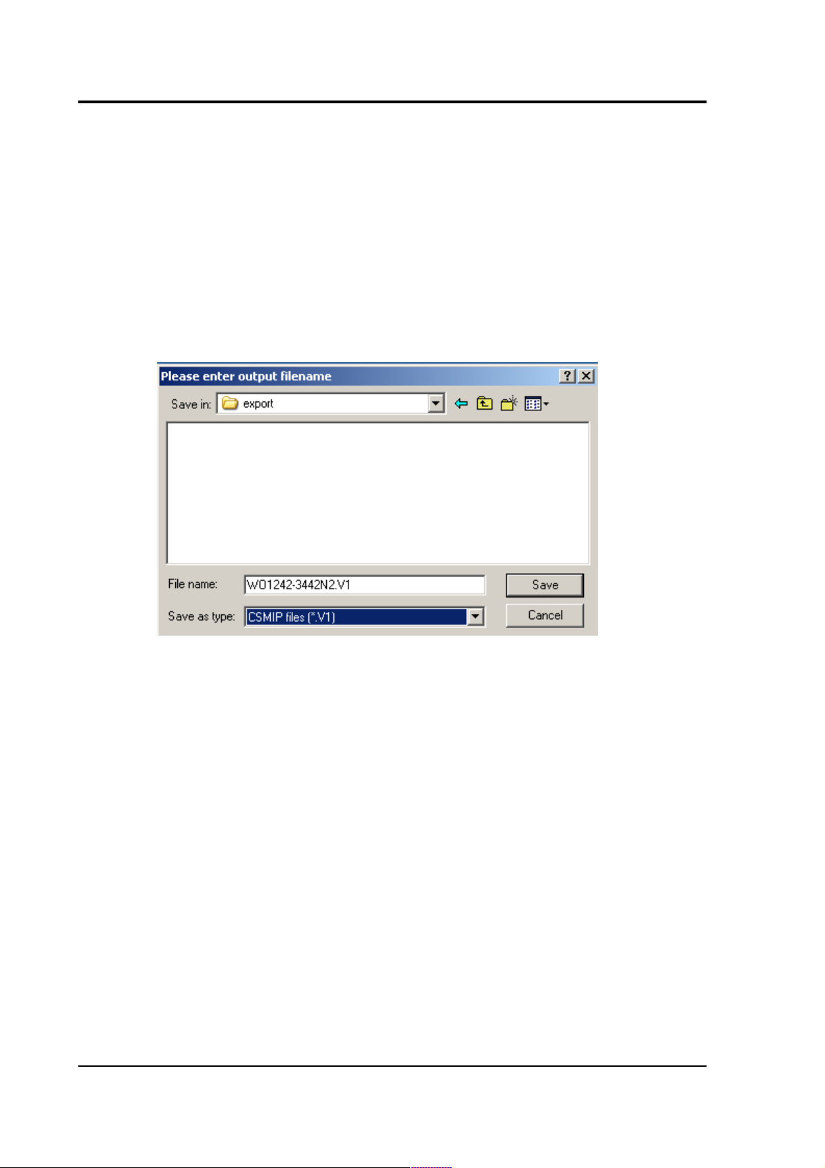
When any of the six buttons are pressed a file selection dialog
box is opened that allows the user to specify the name of the
output file and the extension of this file. The extension must be
given for the program to recognize which data format to export
the data in. A filename is automatically suggested by ART
based on the name listed in the central list box. If the user has
entered metadata concerning the earthquake and station
associated with a time-history these information are included
within the exported files in agreement with the selected file
format. This is a significant improvement with respect to
previous versions of ART.

ISESD

ART allows the exporting of uncorrected and corrected time­histories, response spectra and Fourier amplitude spectra in
the data format of the Internet Site for European Strong-Motion
Data (http://www.isesd.cv.ic.ac.uk) and associated CD-ROM
collections.

When exporting data, choose the file extension for the export
file according to the following table:

24 Issue C

User guide

Type of data being exported file extension to use

uncorrected time-histories

.raw

corrected time-histories

.cor

Fourier amplitude spectra

.fas

elastic response spectra

.spc

input energy spectra

.ene

drift spectra

.ids

SMC

ART allows the exporting of uncorrected and corrected time­histories and response spectra in the SMC data format of the
US National Strong Motion Program
(http://nsmp.wr.usgs.gov/smcfmt.html). When exporting any
form of data use extension .smc. For uncorrected time-histories
and response spectra one output file is created with the
specified name. For corrected time-histories three output files
are created, one with the stem (i.e. the file without the
extension) plus _a.smc (for corrected acceleration), one with
the stem plus _v.smc (for corrected velocity) and one with the
stem plus _d.smc (for corrected displacement).

CSMIP

ART allows the exporting of uncorrected and corrected time­histories and response spectra in the data format of the
California Strong Motion Instrumentation Program
(http://www.conservation.ca.gov/dmg/csmip). When exporting
uncorrected time-histories use extension .v1, when exporting
corrected time-histories use extension .v2 and when exporting
elastic response spectra use extension .v3.

K-NET

ART allows the exporting of uncorrected time-histories in the
data format of Kyoshin-NET in Japan (http://www.k­net.bosai.go.jp/k-net/index_en.shtml). When exporting
uncorrected time-histories use extension .ns, .ew or .ud
depending on the component direction.

PEER

ART allows the exporting of corrected time-histories and
response spectra in the data format of the Pacific Earthquake
Engineering Research Centre (http://peer.berkeley.edu/nga/).

May 2009 25

ART

When exporting corrected time-histories use the extension
.at2 and when exporting response spectra use extension .000.
For corrected time-histories three output files are created, one
with the name specified (for corrected acceleration), one with
the stem specified plus the extension .vt2 (for corrected
velocity) and one with the stem specified plus the extension
.dt2 (for corrected displacement). For response spectra five
output files are created, one with the name specified (for 0%
damping spectrum), one with the stem specified and extension
.020 (for 2% damping spectrum), one with the stem specified
and extension .050 (for 5% damping spectrum), one with the
stem specified and extension .100 (for 10% damping
spectrum) and one with the stem specified and extension .200
(for 20% damping spectrum).

Columns

ART allows the exporting of uncorrected and corrected time­histories, Fourier amplitude spectra, elastic response spectra,
input energy spectra and drift spectra in a column ASCII format.
When exporting files in this format use extension .txt.

SAC

ART allows the exporting of uncorrected and corrected time­histories in the data format of the Seismic Analysis Code
(http://www.llnl.gov/sac/). When exporting files in this format
use extension .sac.

Microsoft Excel

ART allows the exporting of uncorrected and corrected time­histories, Fourier amplitude spectra, elastic response spectra,
input energy spectra and drift spectra in Microsoft Excel .xls
format. When exporting files in this format use extension .xls.

Note that to able to successfully export files in Microsoft Excel
format Excel itself must be installed on the user’s computer

.

Matlab

ART allows the exporting of uncorrected and corrected time­histories, Fourier amplitude spectra, elastic response spectra,
input energy spectra and drift spectra in Matlab native .mat
format. When exporting files in this format use extension .mat.

3.2.7 Clear time-histories

The ‘Clear time-histories’ button clears all the opened time­histories from memory. A confirmation dialog-box asks the user

26 Issue C

User guide

whether they are sure that they wish to clear all the time­histories from memory. Clicking on ‘Yes’ clears the time­histories and clicking on ‘No’ retains the time-histories in
memory.

3.2.8 Event Manager

This feature will be fully documented in Revision D of this
manual. Please contact [e-mail] for further
information.

3.2.9 ‘Unfiltered?’ check box

For each time-history in ART’s memory, either the unfiltered or
filtered (if filtering has been applied) data can be used. If the
‘Unfiltered?’ check box is ticked then the unfiltered version of
the time-history will be selected. Once filtering has been
applied to the selected time-history then the ‘Unfiltered?’ check
box will be un-ticked. To return to the unfiltered version simply
click in the check box to tick the box again. To then return to
the filtered version click in the check box again.

3.2.10 Central list box

This box lists those time-histories currently loaded into ART. If
the time-histories were selected in SCREAM then the time­histories are referred to by their work order and digitizer
number. If the time-histories were loaded through the ‘Import
data’ file selection window the time-histories are referred to by
their filename.

In addition, the time-histories are allocated a unique six-digit
identity number and a letter indicating the component direction
so that they can be used by the ART database. The files are
listed in the order in which they were imported into ART.

Clicking on time-histories' names will select those records to be
processed and analyzed. Multiple time-histories can be
selected for processing and analysis by holding down either the
Ctrl or Shift keys. Clicking on two or three time-histories from
the same record will activate the ‘Particle motions’ button to
enable the plotting of the motion of a particle (hodogram) at
the station. Clicking on time-histories with associated
earthquake and station metadata will active the ‘View time­histories on map’ button to enable the plotting of the time­histories on a map and also the ‘Comparisons’ button to enable

May 2009 27

ART

comparisons between the observed response spectra and
predictions by GMPEs and seismic design codes.

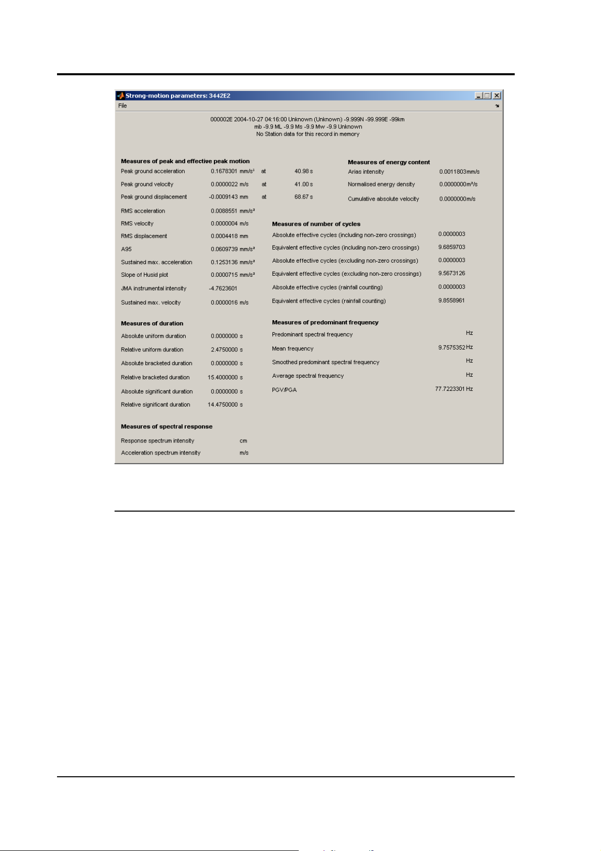
3.2.11 Strong-motion parameters

Clicking on the ‘Strong-motion parameters’ button opens
windows displaying a selection of strong-motion parameters for
the selected time-histories. The parameters that are displayed
are (divided into the characteristic of the motion that the
parameter seeks to measure):

1. peak ground acceleration (PGA) in selected
acceleration units and the time at which this occurs;

2. peak ground velocity (PGV) in selected velocity units
and the time at which this occurs;

3. peak ground displacement (PGD) in selected
displacement units and the time at which this occurs;

4. RMS acceleration in selected acceleration units
calculated from

where T is length of record and a(t) is ground
acceleration;

5. RMS velocity in selected velocity units calculated from

where T is length of record and v(t) is ground velocity;

6. RMS displacement in selected displacement units
calculated from

where T is length of record and d(t) is ground
displacement;

7. A95 parameter in selected acceleration units, which is
defined by Sarma & Yang (1987) as the level of
acceleration that contains up to 95% of the total Arias
intensity;

28 Issue C

A

RMS

=



∫

at2dt

T



1/ 2

V

RMS

=



∫

vt 2dt

T



1/ 2

D

RMS

=



∫

d t 2dt

T



1/ 2

User guide

8. sustained maximum acceleration in selected

acceleration units, which is defined by Nuttli (1979) as
the third (user-defined) highest absolute peak in the
acceleration time-history;

9. slope of Husid plot in selected acceleration units,

which is defined as the slope of the Arias intensity plot
(Husid plot) between user-defined percentages (those
used for calculation of the relative significant
duration) of the total Arias intensity (Bommer et al.,

2004);

10. .Japan Meteorological Agency (JMA) instrumental

intensity, which is defined in
http://www.hp1039.jishin.go.jp/eqchreng/at2-4.htm
(see also Sokolov & Furumura, 2008) based on band­filtered acceleration time-histories (N.B. JMA
instrumental intensity is usually defined for three
orthogonal components but in ART it is computed for
each component individually);

11. sustained maximum velocity in selected velocity

units, which is defined by Nuttli (1979) as the third
(user-defined) highest absolute peak in the velocity
time-history;

12. absolute uniform duration in seconds, which is the

total time that the square of the ground acceleration
is above the square of the ground acceleration
specified in the ‘Options’ window;

13. relative uniform duration in seconds, which is the total

time that the square of the ground acceleration is
above the proportion specified in the ‘Options’ window
of the square of the PGA;

14. absolute bracketed duration in seconds, which is the

interval between the first and last instants where the
square of the ground acceleration exceeds that
specified in the ‘Options’ window;

15. relative bracketed duration in seconds, which is the

interval between the first and last instants where the
ground acceleration exceeds a proportion (specified in
the ‘Options’ window) of the maximum absolute
acceleration.

May 2009 29

ART

16. absolute significant (effective) duration in seconds,
which is the interval between the Arias intensity
exceeding an absolute threshold specified in the
‘Options’ window (‘Significant Absolute (Begin)’) and
the Arias intensity exceeding the total Arias intensity
minus another threshold specified in the ‘Options’
window (‘Significant Absolute (End)’) (Bommer &
Martinez-Pereira, 1999).

For example, if the thresholds are given as 0.1 and

0.125ms-1 then the duration is given as the interval
between the Arias intensity exceeding for the first
time 0.1ms-1 to the total Arias intensity (e.g 0.5)
minus 0.125ms-1 (e.g. 0.375);

17. relative significant duration in seconds, which is the
interval between the proportion of Arias intensity
exceeding that specified in the ‘Options’ window
(‘Significant Relative (Begin)’) and the proportion of
Arias intensity exceeding that specified in the
‘Options’ window (‘Significant Relative (End)’).

18. response spectrum intensity (SI) in selected
displacement units calculated from

with the limits specified in ‘Options’ window, where
PSV(5%,T) is pseudo-spectral velocity for 5% damping
and T is natural period [see Kramer (1996, p. 83)]
(note that this parameter is only calculated if the
response spectrum of the time-history has already
been calculated. The response spectra calculation
must be run again if the limits given in the ‘Options’
window are changed after the response spectra
calculation was made);

19. acceleration spectrum intensity (ASI) in selected
velocity units calculated from

with the limits specified in ‘Options’ window, where
SA(5%,T) is spectral acceleration for 5% damping and
T is natural period [see Kramer (1996, p. 83)] (note
that this parameter is only calculated if the response
spectrum of the time-history has already been

30 Issue C

SI =∫PSV 5% ,T dT

ASI =∫SA 5% , dT

User guide

calculated. The response spectra calculation must be
run again if the limits given in the ‘Options’ window
are changed after the response spectra calculation
was made);

20. Arias intensity (AI) in velocity units based on the

selected acceleration unit calculated from

where g is acceleration due to gravity in ms-2 (i.e.
g=9.80665ms-2) and a(t) is ground acceleration (Arias,

1970);

21. normalized energy density (ED) in units based on the

selected velocity unit calculated from

where v(t) is ground velocity [see Sarma (1971)] [note
that, to get the true energy density, the normalized
energy density should be multiplied by Vρ/4 where V
is wave velocity and ρ is mass density of the
recording site (Sarma, 1971)];

22. cumulative absolute velocity (CAV) in selected

velocity units calculated from

where

a(t)

is the ground acceleration, N is the number

of 1-second time windows in the time series,

PGA

i

is

the PGA (in g) during time window i,

t

i

is the start time

of time window i,

a

min

is an acceleration threshold
(user-defined but commonly 0.025g) to exclude low
amplitude motions contributing to the sum and

H(x)

is
the Heaviside step function (unity for x>0 and 0
otherwise) (EPRI, 2006);

23. number of absolute effective cycles (peak counting
including non-zero crossings) in acceleration time­history (Hancock & Bommer, 2005);

24. number of equivalent effective cycles using user­defined damage exponent (peak counting including
non-zero crossings) in acceleration time-history
(Hancock & Bommer, 2005);

May 2009 31

AI =



2g

∫

at2dt

ED=∫vt2dt

CAV =

∑

i=1

N

H  PGAi−a

min



∫

t=t

i

t

i 1

∣at ∣ dt

ART

25. number of absolute effective cycles (peak counting
excluding non-zero crossings) in acceleration time­history (Hancock & Bommer, 2005);

26. number of equivalent effective cycles using user­defined damage exponent (peak counting excluding
non-zero crossings) in acceleration time-history
(Hancock & Bommer, 2005);

27. number of absolute effective cycles (rainflow counting
technique) in acceleration time-history (Hancock &
Bommer, 2005);

28. number of equivalent effective cycles using user­defined damage exponent (rainflow counting
technique) in acceleration time-history (Hancock &
Bommer, 2005);

29. predominant spectral period (or frequency) defined by
Rathje et al. (2004) as the period at which the
maximum spectral acceleration (using user-defined
damping level) occurs;

30. mean period (or frequency) defined by Rathje et al.
(2004) as:

where

C

i

are Fourier amplitudes at frequencies

f

i

;

31. smoothed predominant spectral period (or frequency)
defined by Rathje et al. (2004) as:

for T

i

with SA/PGA≥ 1.2 where T

i

are periods at which
the spectral accelerations SA are defined (using user­defined damping level);

32 Issue C

Tm=

∑

i

C

i

2

 1/ fi

∑

i

C

i

2

T0=

∑

i

Tiln

[

SATi

PGA

]

∑

i

ln

[

SA Ti

PGA

]

User guide

32. average spectral period (or frequency) defined by

Rathje et al. (2004): .

33. PGV/PGA in seconds (or Hz) (the ratio is computed

using ms-1 for PGV and ms-2 for PGA), which gives an
indication of the period (or frequency) content of the
time-history;

At the top of this window there is a menu entitled ‘File’ with
three options: ‘Save figure’, which saves a copy of the window
as a graphics file (in .bmp, .eps, .jpg, .png or .tif format);
‘Print figure’, which prints a copy of the window; and ‘Export
values’, which exports the strong-motion parameters to a text
file in a space-delimited format.

Also given as a header to the strong-motion parameter table (if
the ‘Display metadata’ option is selected in the ‘Options’
window) are the basic earthquake, station and waveform
metadata corresponding to the selected time-history (if
available).

A typical strong motion analysis screen is shown overleaf.

May 2009 33

ART

3.2.12 View time-histories

Clicking on this button displays the time-histories of the record
that is currently selected (uncorrected if the ‘Unfiltered?’ check
box is ticked and corrected if the ‘Unfiltered?’ check box is
unticked) (see below).

If a single component is selected (or components from different
instruments or with different start times) then the acceleration,
velocity and displacement time-histories of each time-history
are displayed in separate windows. If two or three components
from the same instrument and the same start time are selected
then clicking on this button displays the acceleration time­histories of the selected components in a single window. If the
user requested to display the absolute time of the record this is
displayed as a second x-axis on the figure. The accelerations,
velocities and displacements are displayed using their selected
units.

34 Issue C

User guide

Also shown in this figure (if the ‘Display metadata’ option is
selected in the ‘Options’ window) are the basic earthquake,
waveform and station metadata of the selected time-history (if
available).

The user can zoom in on the three sub-figures by drawing a
bounding box or by clicking on the sub-figures (the sub-figures
are linked together so zooming in on one retains the correct
time relation between the three sub-figures). To zoom out
again, right-click.

At the top of this window there is a menu called ‘File’ with two
items: ‘Save figure’, which saves a copy of the window as a
graphics file (in .bmp, .eps, .jpg, .png or .tif format) and
‘Print figure’, which prints a copy of the window. In addition,
there is a menu called ‘Options’ that allows the user to modify
the variable plotted (acceleration, velocity or displacement),
the units used and whether to display grid lines on the figures.
Changes made here to these options are local and do not affect
the global options that can be modified in the Options window
discussed above.

May 2009 35

ART

3.2.13 View time-histories on map

If the user has entered earthquake and station metadata for
the selected time-histories, the ‘View time-histories on map’
button is enabled. Clicking on this button produces a map
displaying the selected time-histories (only those for the same
earthquake as the first time-history selected in the central list­box and for the component direction selected in the ‘Options’
window) at their geographical positions. In addition, the
epicenter of the earthquake is indicated as an asterisk as are
range rings (if this option is selected in the ‘Options’ window)
marking epicentral distances of 1, 2, 5, 10, 20, 50, 100, 200,
500 and 1000km.

At the top of this window there is a menu called ‘File’ with two
items: ‘Save figure’, which saves a copy of the window as a
graphics file (in .bmp, .eps, .jpg, .png or .tif format) and
‘Print figure’, which prints a copy of the window. Also at the top
of the window there is a menu called ‘Options’ that allows the
user to modify the drawing options of this figure.

36 Issue C

User guide

Also shown in this figure (if the ‘Display metadata’ option is
selected in the ‘Options’ window) are the basic earthquake,
waveform and station metadata of the selected time-history.

3.2.14 Particle motions

When two or three components of the same record are
selected the particle motions button becomes active. Clicking
on this button produces a plot of the motion of a particle
(hodogram) at the station using the acceleration, velocity and
displacement of the two or three time-histories.

If two time-histories are selected a 2D plot is created with three
graphs:

• the left-hand graph shows the acceleration of the first

component (on the x-axis) against the acceleration of
the second component (on the y-axis);

• the middle graph shows the velocity of the first

component (on the x-axis) against the velocity of the
second component (on the y-axis); and

• the right-hand graph shows the displacement of the

first component (on the x-axis) against the
displacement of the second component (on the y-axis).

If three time-histories are selected a 3D plot is created with
three graphs:

• the left-hand graph shows the acceleration of the first

component (on the x-axis) against the acceleration of
the second component (on the y-axis) and the
acceleration of the third component (z-axis);

• the middle graph shows the velocity of the first

component (on the x-axis) against the velocity of the
second component (on the y-axis) and the velocity of
the third component (z-axis); and

• the right-hand graph shows the displacement of the

first component (on the x-axis) against the
displacement of the second component (on the y-axis)
and the displacement of the third component (z-axis).

The order of the components is always the same as that given
in the list of time-histories currently in memory. When three

May 2009 37

ART

components are selected the 3D particle motions plots also
display projections of the motions onto the x-y, x-z and y-z 2D
planes (if requested in the ‘Options’ menu at the top of the
window).

The accelerations, velocities and displacements are displayed
using their selected units. Also shown in this figure (if the
‘Display metadata’ option is selected in the ‘Options’ window)
are the basic earthquake, waveform and station metadata of
the selected time-history.

At the top of this window there is a menu called ‘File’ with two
items: ‘Save figure’, which saves a copy of the window as a
graphics file (in these formats: .bmp, .eps, .jpg, .png or
.tif) and ‘Print figure’, which prints a copy of the window.
Also at the top of the window there is a menu called ‘Options’
that allows the user to modify the drawing options of this
figure.

38 Issue C

User guide

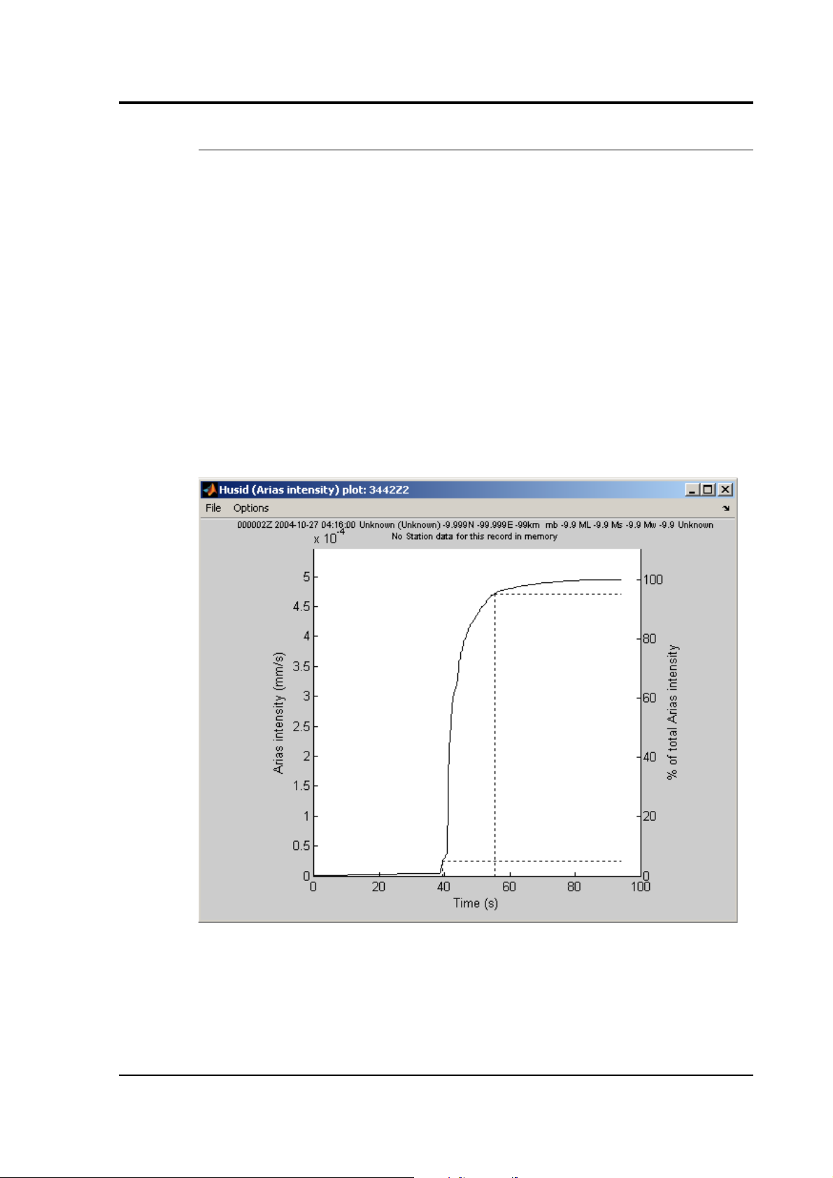
3.2.15 Husid (Arias intensity) plot

As for other functions, this button has two behaviours
depending on whether single or multiple time-histories have
been selected. The windows produced can be saved in different
graphical formats (.bmp, .eps, .jpg, .png or .tif) using the
‘Save figure’ option on the ‘File’ menu and printed using the
‘Print figure’ option the ‘File’ menu. Also the values plotted can
be saved in a column format using the ‘Export data’ option on
the ‘File’ menu. The options used to create the figure can be
changed within the ‘Options’ menu located at the top of the
window.

The Arias intensities are displayed using units based on the
selected acceleration unit.

Single time-history selected

Clicking on this button will calculate and display the Husid plot
(i.e. Arias intensity against time) of the currently selected time­history (see below). The left hand axis gives the Arias intensity
and the right hand side gives the percentage of Arias intensity.

May 2009 39

ART

Also displayed on the graph are dashed lines showing the times
the intensity first exceeds the proportion of final Arias intensity
given in the ‘Options’ window (‘Significant Relative (Start)’ and
‘Significant Relative (End)’.)

Also shown in this figure (if the ‘Display metadata’ option is
selected in the ‘Options’ window) are the basic earthquake,
waveform and station metadata of the selected time-history.

Multiple time-histories selected

Clicking on this button when two or more time-histories are
selected calculates and displays the Husid plots for all the
selected time-histories on the same graph so that they can be
easily compared (see below). The figure is either displayed in
colour or in monochrome depending on the option selected by
the user within the ‘Options’ window.

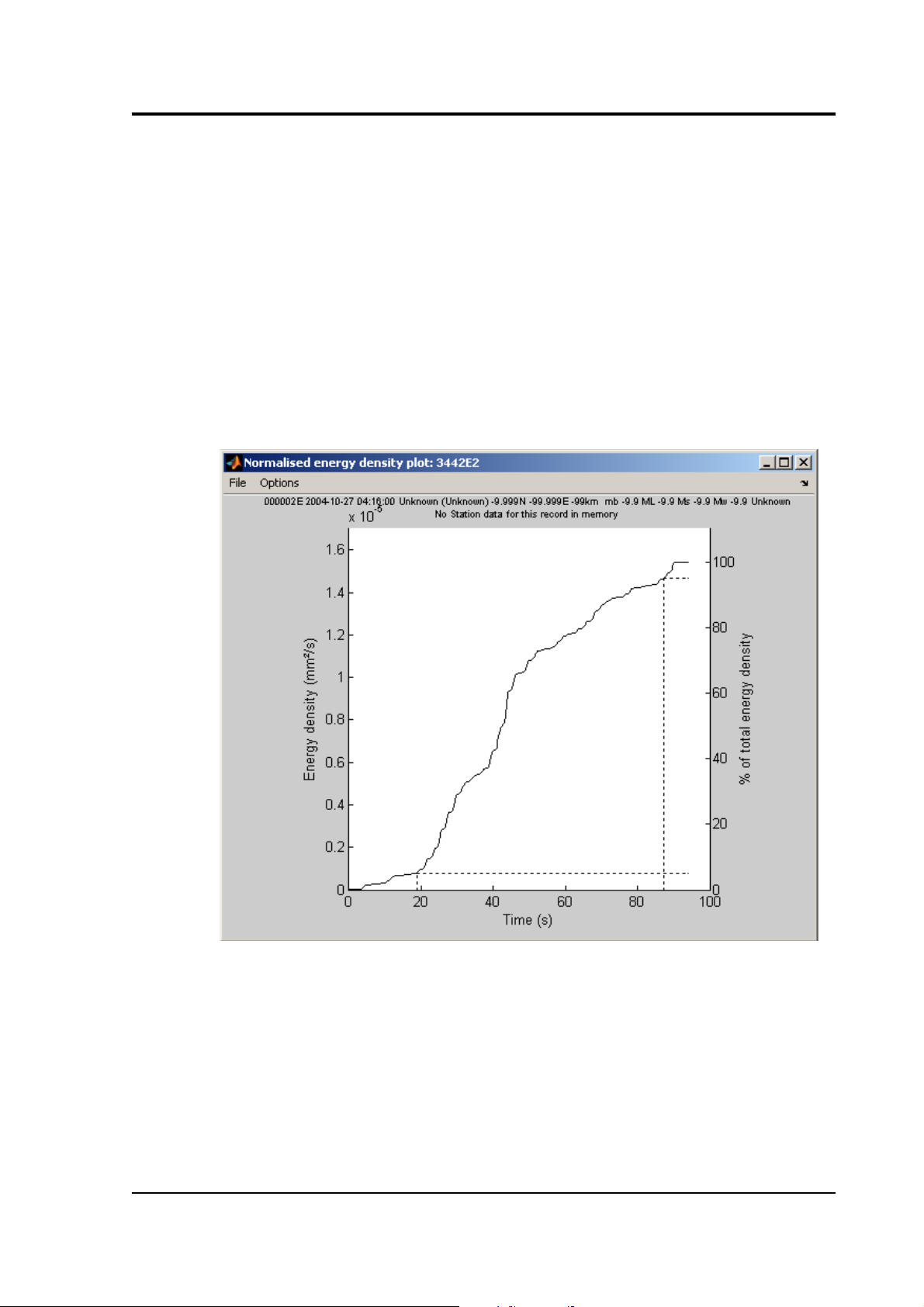
3.2.16 Energy density plot

As for other functions this button also has two behaviours
depending on whether a single or multiple time-histories have
been selected. The windows produced can be saved in different

40 Issue C

User guide

graphical formats (.bmp, .eps, .jpg, .png or .tif) using the
‘Save figure’ option on the ‘File’ menu and printed using the
‘Print figure’ option the ‘File’ menu.

The values plotted can also be saved in a column format using
the ‘Export data’ option on the ‘File’ menu. The options used to
create the figure can be changed within the ‘Options’ menu
located at the top of the window.

The normalized energy densities are displayed using units
based on the selected velocity unit.

Single time-history selected

Clicking on this button will calculate and display the normalized
energy density plot [i.e. energy density against time (Sarma,

1971)] of the currently selected time-history. The left hand axis
gives the normalized energy density [note that, to get the true
energy density, the normalized energy density should be
multiplied by Vρ/4 where V is wave velocity and ρ is mass
density (Sarma, 1971)] and the right hand side gives the
percentage of normalized energy density. Also displayed on the

May 2009 41

ART

graph are dotted lines showing the times the energy density
first exceeds the proportions of final normalized energy density
given in the ‘Options’ window (‘Significant Relative (Start)’ and
‘Significant Relative (End)’).

Also shown in this figure (if the ‘Display metadata’ option is
selected in the ‘Options’ window) are the basic earthquake,
waveform and station metadata of the selected time-history.

Multiple time-histories selected

Clicking on this button when two or more time-histories are
selected calculates and displays the energy density plots for all
the selected time-histories on the same graph so that they can
be easily compared (see below). The figure is either displayed
in colour or in monochrome depending on the option selected
by the user within the ‘Options’ window.

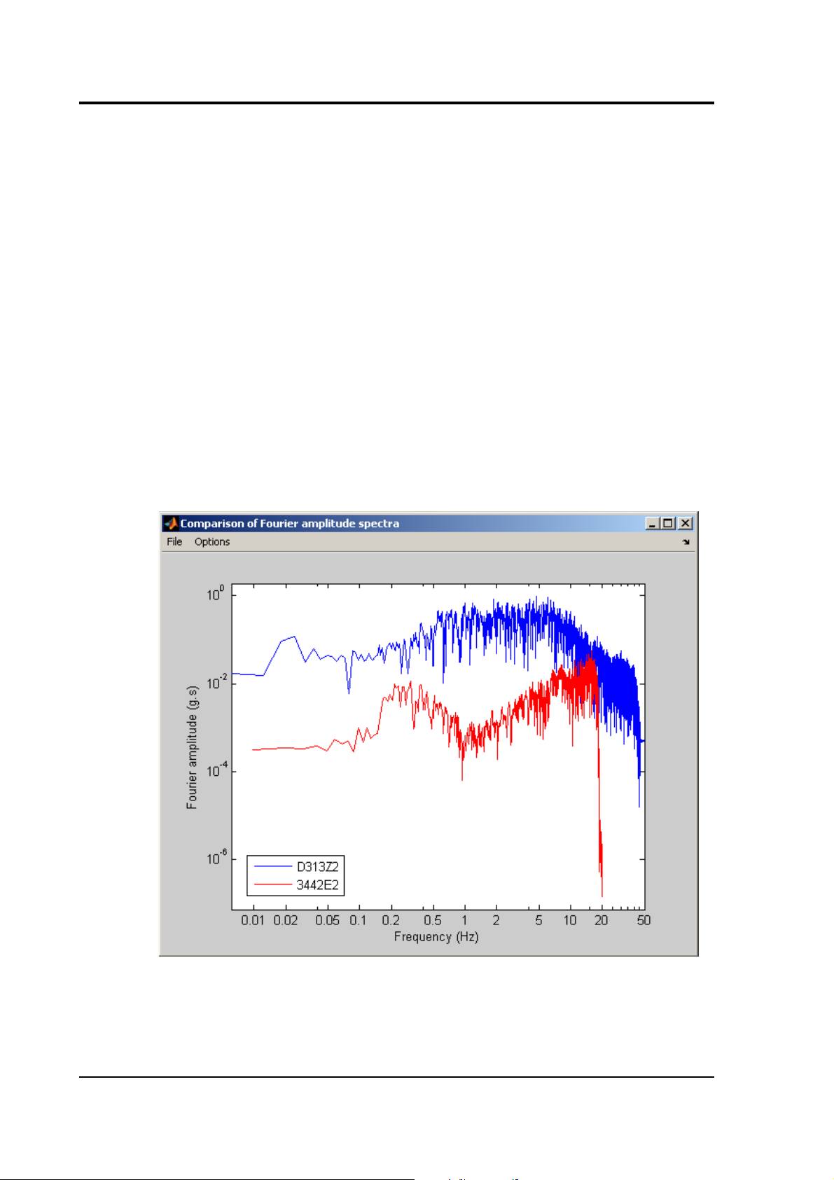
3.2.17 Fourier amplitude spectrum

Like the other buttons, this function has two behaviours
depending on whether single or multiple time-histories have
been selected. The windows produced can be saved in different

42 Issue C

User guide

graphical formats (.bmp, .eps, .jpg, .png or .tif) using the
‘Save figure’ option on the ‘File’ menu and printed using the
‘Print figure’ option the ‘File’ menu. The figures are either
displayed in colour or in monochrome depending on the option
selected by the user within the ‘Options’ window. The options
used to create the figure can be changed within the ‘Options’
menu located at the top of the window.

The Fourier amplitude spectra are displayed using units based
on the selected unit for the selected variable (e.g. a unit based
on the selected acceleration unit is used if the variable chosen
to be displayed is acceleration).

Single time-history selected

Clicking on this button when a single time-history has been
selected will calculate and display the Fourier amplitude
spectrum of the currently selected time-history. No smoothing
of the Fourier amplitude spectrum is applied. Two Fourier
amplitude spectra are calculated: one using the pre-event
portion of the record and one using the remainder of the

May 2009 43

ART

record. Comparing these two spectra enables a choice of the
high-pass cut-off frequency to be made.

The figure above shows an example where a cut-off frequency
of about 1.5Hz is suggested by comparing the two spectra
because for lower frequencies the signal-to-noise ratio is quite
low.

A sub-figure underneath can be requested in the ‘Options’
menu at the top of the figure to show the signal-to-noise
spectral ratio computed using the Fourier amplitude spectra of
the pre-event portion (as an estimate of the noise) and the
remainder of the record (as an estimate of the signal).

Also shown in this figure (if the ‘Display metadata’ option is
selected in the ‘Options’ window) are the basic earthquake,
waveform and station metadata of the selected time-history.

Multiple time-histories selected

Clicking on this button when multiple time-histories have been
selected calculates and plots the Fourier amplitude spectra of

44 Issue C

User guide

the currently selected time-histories for the period after the
pre-event portion of the record.

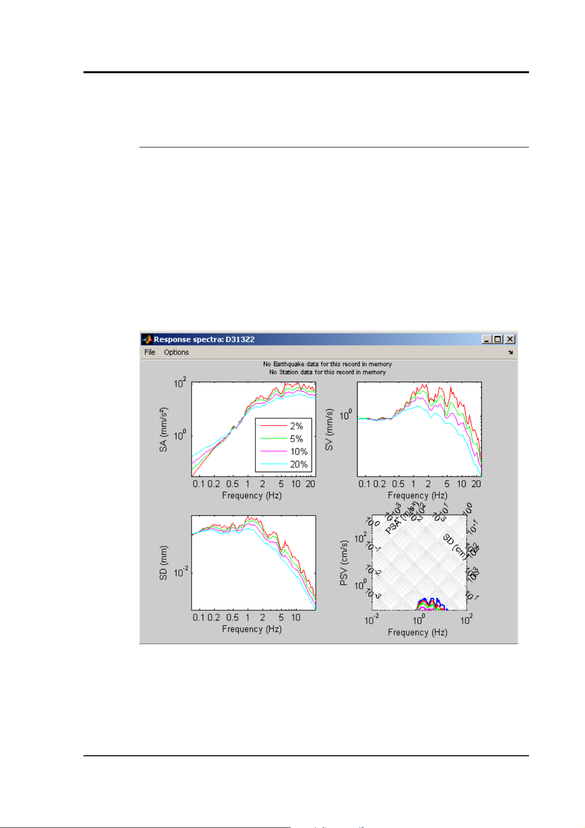
3.2.18 Elastic response spectra

This function has two behaviours, depending on whether single
or multiple time-histories have been selected. The windows
produced can be saved in different graphical formats (.bmp,
.eps, .jpg, .png or .tif) using the ‘Save figure’ option on
the ‘File’ menu and printed using the ‘Print figure’ option the
‘File’ menu. The figures are either displayed in colour or in
monochrome depending on the option selected by the user
within the ‘Options’ window. The options used to create the
figure can be changed within the ‘Options’ menu located at the
top of the window.

Single time-history selected

Clicking on this button when only a single time-history has
been selected calculates and plots the elastic response spectra
of the currently selected time-history for 2, 5, 10 and 20%
damping and periods between 0.04 and 15 seconds. (The un­damped spectra are also computed but are not displayed due

May 2009 45

ART

to their limited applicability in engineering
seismology/earthquake engineering). This calculation takes a
few seconds for a normal length time-history. The method
given in Beaudet & Wolfson (1970) is used to calculate the
spectra. The spectra are plotted on tripartite and standard
(logarithmic or linear, depending on the choice made in the
‘Options’ window) plots for spectral acceleration, spectral
velocity and spectral displacement. The spectra are displayed
using the units selected by the user in the ‘Options’ window.

Also shown in this figure (if the ‘Display metadata’ option is
selected in the ‘Options’ window) are the basic earthquake,
waveform and station metadata of the selected time-history.

Multiple time-histories selected

Clicking on this button when multiple time-histories have been
selected calculates and plots the elastic response spectra of
the currently selected time-histories for the damping level
specified in the ‘Options’ window and displays them on the
same sub-figures so that they can be easily compared (see
below).

46 Issue C

User guide

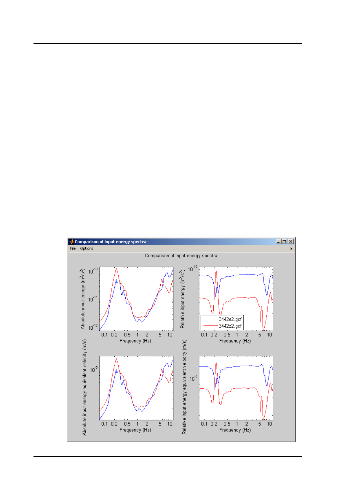
3.2.19 Elastic input energy spectra

This function has two behaviours, depending on whether single
or multiple time-histories have been selected. The windows
produced can be saved in different graphical formats (.bmp,
.eps, .jpg, .png or .tif) using the ‘Save figure’ option on
the ‘File’ menu and printed using the ‘Print figure’ option the
‘File’ menu. The figures are either displayed in colour or in
monochrome depending on the option selected by the user
within the ‘Options’ window. The options used to create the
figure can be changed within the ‘Options’ menu located at the
top of the window.

Single time-history selected

Clicking on this button when only a single time-history has
been selected calculates and plots the elastic absolute and
relative input energy spectra and their equivalent velocities
(e.g. Chapman, 1999) of the currently selected time-history for
2, 5, 10 and 20% damping and periods between 0.04 and 15s.

May 2009 47

ART

The undamped spectra are also computed but are not
displayed due to their limited applicability in engineering
seismology/earthquake engineering. The calculation takes a
few seconds for a normal length time-history. The method
given in Beaudet & Wolfson (1970) is used to calculate the
spectra. The spectra are displayed using the units selected by
the user in the ‘Options’ window and using the other selected
options.

Also shown in this figure (if the ‘Display metadata’ option is
selected in the ‘Options’ window) are the basic earthquake,
waveform and station metadata of the selected time-history.

Multiple time-histories selected

Clicking on this button when multiple time-histories have been
selected calculates and plots the elastic absolute and relative
input energy spectra and their equivalent velocities (e.g.
Chapman, 1999) of the currently selected time-histories for the
damping level specified in the ‘Options’ window and displays
them on the same sub-figures so that they can easily be
compared (see below).

48 Issue C

User guide

3.2.20 Drift spectra

This function has two behaviours depending on whether a
single or multiple time-histories have been selected. The
windows produced can be saved in different graphical formats
(.bmp, .eps, .jpg, .png or .tif) using the ‘Save figure’
option on the ‘File’ menu and printed using the ‘Print figure’
option the ‘File’ menu. The figures are either displayed in
colour or in monochrome depending on the option selected by
the user within the ‘Options’ window. The options used to
create the figure can be changed within the ‘Options’ menu
located at the top of the window.

Single time-history selected

Clicking on this button when only a single time-history has
been selected calculates and plots the drift spectrum (e.g.
Iwan, 1997) of the currently selected time-history for the
selected damping level and material type and periods between

0.5 and 15s (see below). This calculation can take many
seconds for a long time-history. The method given in Wang
(1996) is used to calculate the spectra. The spectra are
displayed in terms of percentage of maximum inter-storey drift.

May 2009 49

ART

Also shown in this figure (if the ‘Display metadata’ option is
selected in the ‘Options’ window) are the basic earthquake,
waveform and station metadata of the selected time-history.

Multiple time-histories selected

Clicking on this button when multiple time-histories have been
selected calculates and plots the drift spectra (e.g. Iwan, 1997)
of the currently selected time-histories for the damping level
and material type specified in the ‘Options’ window and
displays them on the same graph so that they can be easily
compared (see below).

3.2.21 Comparisons

Clicking on this button opens a new window (see below) that
allows the user to compare the observed elastic response
spectra of the selected time-histories with predicted median
spectra from 21 recent GMPEs (e.g. Douglas, 2003) and three
seismic design codes. The GMPEs that can be selected by
clicking on the check-boxes are the following:

1. Abrahamson & Silva (1997) (AS97);

50 Issue C

User guide

2. Ambraseys & Douglas (2003) (AD03);

3. Ambraseys et al. (1996) /
Ambraseys & Simpson (1996) (AETAL96, AS96);

4. Ambraseys et al. (2005a, b) (AETAL05);

5. Atkinson & Boore (1997) (AB97);

6. Atkinson & Boore (2003) (AB03);

7. Berge-Thierry et al. (2003) (BTETAL03);

8. Bindi et al. (2006) (BETAL06);

9. Boore et al. (1997) (BETAL97);

10. Campbell (1997) (C97);

11. Campbell & Bozorgina (2003a, b, c) (CB03);

12. Crouse (1991) (C91);

13. Kalkan & Gülkan (2004) (KG04);

14. Lussou et al. (2001) (LETAL01);

15. Ozbey et al. (2004) (OETAL04);

16. Sabetta & Pugliese (1996) (SP96);

17. Sadigh et al. (1997) (SETAL97);

18. Spudich et al. (1999) (SETAL99);

19. Toro et al. (1997) (TETAL97);

20. Youngs et al. (1997) (YETAL97);

21. Zonno & Montaldo (2002) (ZM02).

Predictions from these GMPEs are only displayed on the
comparison graph if the required metadata (e.g. mechanism
type) is available for the selected time-histories. In addition,
some of the GMPEs are only for horizontal motions and
therefore no predictions are displayed if only vertical

May 2009 51

ART

components are selected. Also, some GMPEs are for specific
site conditions (e.g. rock) and therefore no predictions are
displayed if the selected time-histories were recorded at sites
with different conditions. The user is encouraged to study the
original references [or the summaries by Douglas (2004, 2006,

2008)] for the limits of validity of the models and for which
metadata are required.

The seismic design codes that can be selected are the
following:

1. Eurocode 8 (European Committee for Standardization,

2002) (EC8);

2. Uniform Building Code 1997 (International Conference of
Building Officials, 1997) (UBC1997);

3. International Building Code 2000 (International Code
Council, 2000) (IBC2000).

UBC1997 and IBC2000 do not provide predictions for vertical
spectra and so these are not displayed if the time-histories
selected are for the vertical component. The user is
encouraged to study these references for the limits of the
validity of these seismic design code spectra.

Once the user has selected the GMPEs and the codes to
compare with the observed elastic response spectra for the
selected time-histories (and, if a seismic design code has been

52 Issue C

User guide

selected, entered the necessary information), clicking on the
Compare button opens a new window displaying the predicted
and observed spectra (see below). The predicted spectra are
referred to by the abbreviations given above.

May 2009 53

ART

4 References

Abrahamson, N. A., & Silva, W. J. (1997),

Empirical response

spectral attenuation relations for shallow crustal earthquakes

.

Seismological Research Letters, 68(1), 94–127.

Ambraseys, N. N., & Douglas, J. (2003),

Near-field horizontal

and vertical earthquake ground motions

. Soil Dynamics and

Earthquake Engineering, 23(1), 1–18.

Ambraseys, N. N., & Simpson, K. A. (1996),

Prediction of

vertical response spectra in Europe

. Earthquake Engineering

and Structural Dynamics, 25(4), 401–412.

Ambraseys, N. N., Simpson, K. A., & Bommer, J. J. (1996),

Prediction of horizontal response spectra in Europe

. Earthquake

Engineering and Structural Dynamics, 25(4), 371–400.

Ambraseys, N. N., Douglas, J., Sarma, S. K., & Smit, P. M.
(2005a),

Equations for the estimation of strong ground motions
from shallow crustal earthquakes using data from Europe and
the Middle East: Horizontal peak ground acceleration and
spectral acceleration

. Bulletin of Earthquake Engineering, 3(1),

1–53.

Ambraseys, N. N., Douglas, J., Sarma, S. K., & Smit, P. M.
(2005b),

Equations for the estimation of strong ground motions
from shallow crustal earthquakes using data from Europe and
the Middle East: Vertical peak ground acceleration and spectral
acceleration

. Bulletin of Earthquake Engineering, 3(1), 55–73.

Arias, A. (1970),

A measure of earthquake intensity, Seismic

Design for Nuclear Power Plants (ed. R.J. Hansen)

, MIT Press,

Cambridge, Massachusetts, 438-483.

Atkinson, G. M. and Boore, D. M. (1997),

Some comparisons

between recent ground-motion relations

. Seismological

Research Letters, 68(1), 24–40.

Atkinson, G. M., & Boore, D. M. (2003),

Empirical ground­motion relations for subduction zone earthquakes and their
application to Cascadia and other regions

. Bulletin of the

Seismological Society of America, 93(4), 1703–1729.

54 Issue C

User guide

Beaudet, P. R. & Wolfson, S. J. (1970),

Digital filters for

response spectra

, Bulletin of the Seismological Society of

America, 60(3), 1001-1013.

Berge-Thierry, C., Cotton, F., Scotti, O., Griot-Pommera, D.-A., &
Fukushima, Y. (2003),

New empirical response spectral

attenuation laws for moderate European earthquakes

. Journal

of Earthquake Engineering, 7(2), 193–222.

Bindi, D., Luzi, L., Pacor, F., Franceshina, G., & Castro, R. R.
(2006),

Ground-motion predictions from empirical attenuation
relationships versus recorded data: The case of the 1997–1998
Umbria-Marche, central Italy, strong-motion data set

. Bulletin of

the Seismological Society of America, 96(3), 984–1002.

Bommer, J. J. & Martinez-Pereira (1999),

The effective duration

of earthquake strong motion

, Journal of Earthquake

Engineering, 3(2), 127-172.

Bommer, J. J., Magenes, G., Hancock, J., Penazzo, P. (2004),

The
influence of strong motion duration on the seismic response of
masonry structures

, Bulletin of Earthquake Engineering, 2(1),

1-26. DOI: 10.1023/B:BEEE.0000038948.95616.bf.

Boore, D. M., Joyner, W. B., & Fumal, T. E. (1997),

Equations for
estimating horizontal response spectra and peak acceleration
from western North American earthquakes: A summary of
recent work

. Seismological Research Letters, 68(1), 128–153.

Campbell, K. W. (1997),

Empirical near-source attenuation
relationships for horizontal and vertical components of peak
ground acceleration, peak ground velocity, and pseudo­absolute acceleration response spectra

. Seismological

Research Letters, 68(1), 154–179.

Campbell, K. W., & Bozorgnia, Y. (2003a),

Updated near-source
ground-motion (attenuation) relations for the horizontal and
vertical components of peak ground acceleration and
acceleration response spectra

. Bulletin of the Seismological

Society of America, 93(1), 314–331.

Campbell, K. W., & Bozorgnia, Y. (2003b),

Erratum: Updated
near-source ground-motion (attenuation) relations for the
horizontal and vertical components of peak ground
acceleration and acceleration response spectra

. Bulletin of the

Seismological Society of America, 93(3), 1413.

May 2009 55

ART

Campbell, K. W., & Bozorgnia, Y. (2003c),

Erratum: Updated
near-source ground-motion (attenuation) relations for the
horizontal and vertical components of peak ground
acceleration and acceleration response spectra

. Bulletin of the

Seismological Society of America, 93(4), 1872.

Chapman, M. C. (1999),

On the use of elastic input energy for

seismic hazard analysis

, Earthquake Spectra, 15(4), 607-635.

Consortium of Organizations for Strong-Motion Observation
Systems (2001),

COSMOS Strong Motion Data Format

, Version

1.20, August 15.

Converse, A. M. & Brady, A.G. (1992),

BAP: Basic Strong-Motion

Accelerogram Processing Software Version 1.0

, Open-File

Report 92-296A, U.S. Geological Survey.

Crouse, C. B. (1991),

Ground-motion attenuation equations for

earthquakes on the Cascadia subduction zones

. Earthquake

Spectra, 7(2), 201–236.

Douglas, J. (2003),

Earthquake ground motion estimation using
strong-motion records: A review of equations for the estimation
of peak ground acceleration and response spectral ordinates

.

Earth-Science Reviews, 61(1-2), 43–104.

Douglas, J. (2004a),

Ground motion estimation equations 1964–
2003: Reissue of ESEE Report No. 01-1: ‘A comprehensive
worldwide summary of strong-motion attenuation relationships
for peak ground acceleration and spectral ordinates (1969 to

2000)’ with corrections and additions

. Technical Report 04-001­SM, Department of Civil and Environmental Engineering;
Imperial College of Science, Technology and Medicine; London;
U.K.

Douglas, J. (2006),

Errata of and additions to ‘Ground motion

estimation equations 1964–2003’

. Intermediary report RP-

54603-FR, BRGM, Orléans, France.

Douglas, J. (2008),

Further errata of and additions to ‘Ground

motion estimation equations 1964-2003’

. Final report RP-

56187-FR, BRGM, Orléans, France.

Electric Power Research Institute (2006),

Program on
Technology Innovation: Use of Cumulative Absolute Velocity
(CAV) in Determining Effects of Small Magnitude Earthquakes

56 Issue C

User guide

on Seismic Hazard Analyses

. EPRI, Palo Alto, CA, and the U.S.

Department of Energy, Germantown, MD: 2006 1014099.

European Committee for Standardization (2002).

Eurocode 8:
Design of structures for earthquake resistance Part 1: General
rules, seismic actions and rules for buildings

. Tech. rept. Doc
CEN/TC250/SC8/N317. Central Secretariat: rue de Stassart 36,
B1050 Brussels.

Hancock, J. & Bommer, J. J. (2005),

The effective number of

cycles of earthquake ground motion

, Earthquake Engineering &

Structural Dynamics, 34, 637-664.

International Code Council, Inc. (2000). 2000

International

Building Code. USA

: International Code Council, Inc.

International Conference of Building Officials (1997).

1997

Uniform Building Code. Vol. 2

. Whittier, USA: International

Conference of Building Officials.

Internet Site for European Strong-Motion Data (2002),
http://www.isesd.cv.ic.ac.uk

Iwan, W. D. (1997),

The drift spectrum: a measure of demand

for earthquake ground motions

. Journal of Structural

Engineering (ASCE), 123, 397–404.

K-NET (2002),

About K-NET data format

, http://www.k-

net.bosai.go.jp/k-net/man/knetform_en.html

Kramer, S. L. (1996),

Geotechnical Earthquake Engineering

,

Prentice Hall.

Kalkan, E., & Gülkan, P. (2004),

Site-dependent spectra derived

from ground motion records in Turkey

. Earthquake Spectra,

20(4), 1111–1138.

Lussou, P., Bard, P. Y., Cotton, F., & Fukushima, Y. (2001),

Seismic design regulation codes: Contribution of K-Net data to
site effect evaluation

. Journal of Earthquake Engineering, 5(1),

13–33.

National Strong-Motion Program (2002),

SMC-format Data files

,

http://nsmp.wr.usgs.gov/smcfmt.html

Nuttli, O.W. (1979),

The relation of sustained maximum ground

acceleration and velocity to earthquake intensity and

May 2009 57

ART

magnitude

, Miscellaneous Paper S-71-1, Report 16, U.S. Army
Corps of Engineers, Waterways Experiment Station, Vicksburg,
Mississippi. Not seen.

Ozbey, C., Sari, A., Manuel, L., Erdik, M., & Fahjan, Y. (2004),

An empirical attenuation relationship for northwestern Turkey
ground motion using a random effects approach

. Soil Dynamics

and Earthquake Engineering, 24, 115–125.

PEER Strong Motion Database (2002), http://peer.berkeley.edu/
smcat/data.html.

Rathje, E.M., Faraj, F., Russell, S., & Bray, J.D. (2004),

Empirical
relationships for frequency content parameters of earthquake
ground motions

, Earthquake Spectra, 20(1), 119-144.

Sabetta, F., & Pugliese, A. (1996),

Estimation of response
spectra and simulation of nonstationary earthquake ground
motions

. Bulletin of the Seismological Society of America,

86(2), 337–352.

Sadigh, K., Chang, C.-Y., Egan, J. A., Makdisi, F., & Youngs, R. R.
(1997),

Attenuation relationships for shallow crustal

earthquakes based on California strong motion data

.

Seismological Research Letters, 68(1), 180–189.

Sarma, S. K. (1971),

Energy flux of strong earthquakes

,

Tectonophysics, 11, 159-173.

Sarma, S. K. & Yang, K. S. (1987),

An evaluation of strong

motion records and a new parameter A95

, Earthquake

Engineering & Structural Dynamics, 15(1), 119-132.

Shakal, A. F. & Huang, M. J. (1985),

Standard tape format for

CSMIP strong-motion data tapes

, California Strong Motion

Instrumentation Program, Report OSMS 85-03.

Sokolov, V. & Furumura, T. (2008),

Comparative analysis of two
methods for instrumental intensity estimations using the
database accumulated during recent large earthquakes in
Japan

, Earthquake Spectra, 24(2), 513-532.

Spudich, P., Joyner, W. B., Lindh, A. G., Boore, D. M., Margaris,
B. M., & Fletcher, J. B. (1999), SEA99:

A revised ground motion

prediction relation for use in extensional tectonic regimes

.

Bulletin of the Seismological Society of America, 89(5), 1156–

1170.

58 Issue C

User guide

Toro, G.R., Abrahamson, N.A. & Schneider, J.F. (1997).

Model of
strong ground motions from earthquakes in Central and
Eastern North America: Best estimates and uncertainties

.

Seismological Research Letters 68(1), 41-57.

Wang, L.-J. (1996),

Processing of near-field earthquake

accelerograms, Report no. EERL 96-04

, Earthquake Engineering
Research Laboratory, California Institute of Technology,
Pasadena, USA.

Youngs, R. R., Chiou, S.-J., Silva, W. J., & Humphrey, J. R.
(1997).

Strong ground motion attenuation relationships for

subduction zone earthquakes

. Seismological Research Letters,

68(1), 58–73.

Zonno, G., & Montaldo, V. (2002).

Analysis of strong ground

motions to evaluate regional attenuation relationships

. Annals

of Geophysics, 45(3–4), 439–454.

May 2009 59

ART

5 Software Change History

5.1 Changes from ART 2

• Multiple time-histories can be selected for importation

into ART.

• Absolute and relative input energy spectra can be

computed, plotted and exported.

• Drift spectra for a cantilever shear-beam can be

computed, plotted and exported.

• Various strong-motion parameters based on cycle

counting can be computed and exported.

• Various additional strong-motion parameters can be

computed and exported.

• Graphs can be customized in more ways compared to

ART2.0.

• Records and derived parameters can be exported in

Microsoft Excel .xls and Matlab .mat format.

• Basic database functionality was added so that

earthquake and station meta-data can be recorded and
used.

• Comparisons can be made between observed elastic

response spectra and spectra predicted by various
ground-motion prediction equations (GMPEs) and seismic
design codes.

• Time-histories can be plotted on to maps to show the

geographical distribution of ground motions.

• The software now supports accessing modem-connected

instruments.

• The code was made more efficient leading to better

performance.

• The software was made more user-friendly.

60 Issue C

User guide

5.2 Changes from ART 1

• Adjusted absolute time of record to account for zero-

padding added before instrument correction and filtering
in display and when exporting.

• Added ability to export all derived strong-motion

parameters (e.g. Arias intensity and Fourier amplitudes).

• Correction for instrument response is now performed

automatically when a time-history is loaded.

• Added ability to process and view many records at once.

• Comparisons between derived parameters (e.g. response

spectral ordinates) from different records can by made.

• Added zoom in and out functionality to time-history

windows.

• Graphs can now be exported in a variety of graphical

formats (formats supported are: .bmp, .eps, .jpg, .png
and .tif).

• Graphs can now be printed.

• Time-histories and derived strong-motion parameters can

be displayed using different units.

• Data from instruments with a velocity response can be

imported, converted to acceleration and processed
appropriately.

• A filename is automatically suggested for the export of

time-histories and derived parameters.

• Some minor bugs were corrected.

• The appearance of some windows was improved.

• Options have been add to allow the user to customize the

appearance and functioning of some features.

• The code was made more efficient leading to slightly

better performance.

May 2009 61

ART

• The polarity of the peak ground motion parameters is

now displayed.

• The absolute significant (effective) duration is now

computed.

• The cut-off frequency and order of the high-pass

Butterworth filter can be chosen interactively using
Fourier amplitude spectra of the signal and the noise
(estimated from the pre-event portion of the time­history).

• The units used to display accelerations, velocities and

displacements can be chosen.

62 Issue C

User guide

6 Revision history

2009-04-21 C Rewritten for ART 3.0

2006-09-25 B Rewritten for ART 2.0

2006-04-28 A Added revision history

May 2009 63