

Page 1

Page 2

Copyright© 2003-2015 Geophysical Survey Systems, Inc.
All rights reserved
including the right of reproduction
in whole or in part in any form
Published by Geophysical Survey Systems, Inc.
40 Simon Street
Nashua, New Hampshire 03060-3075 USA
Printed in the United States
SIR, RADAN and UtilityScan are registered trademarks of Geophysical Survey Systems, Inc.
Page 3

Geophysical Survey Systems, Inc. hereinafter referred to as GSSI, warrants that for a period of
24 months from the delivery date to the original purchaser this product will be free from defects
in materials and workmanship. EXCEPT FOR THE FOREGOING LIMITED WARRANTY,
GSSI DISCLAIMS ALL WARRANTIES, EXPRESS OR IMPLIED, INCLUDING ANY
WARRANTY OF MERCHANTABILITY OR FITNESS FOR A PARTICULAR PURPOSE.
GSSI's obligation is limited to repairing or replacing parts or equipment which are returned to
GSSI, transportation and insurance pre-paid, without alteration or further damage, and which in
GSSI's judgment, were defective or became defective during normal use.
GSSI ASSUMES NO LIABILITY FOR ANY DIRECT, INDIRECT, SPECIAL, INCIDENTAL
OR CONSEQUENTIAL DAMAGES OR INJURIES CAUSED BY PROPER OR IMPROPER
OPERATION OF ITS EQUIPMENT, WHETHER OR NOT DEFECTIVE.
Before returning any equipment to GSSI, a Return Material Authorization (RMA) number must
be obtained. Please call the GSSI Customer Service Manager who will assign an RMA number.
Be sure to have the serial number of the unit available
This device complies with Part 15 of the FCC Rules. Operation is subject to the following two
conditions: (1) this device may not cause harmful interference, and (2) this device must accept
any interference received, including interference that may cause undesired operation.
Warning: Changes or modifications to this unit not expressly approved by the party responsible
for compliance could void the user’s authority to operate the equipment.
Note: This equipment has been tested and found to comply with the limits for a Class B digital
device, pursuant to Part 15 of the FCC Rules. These limits are designed to provide reasonable
protection against harmful interference when the equipment is operated in a commercial
environment or residential installation. This equipment generates, uses, and can radiate radio
frequency energy and, if not installed and used in accordance with the introduction manual, may
cause harmful interference to radio communications. However, there is not guarantee that
interference will not occur in a particular installation.
Shielded cables must be used with this unit to ensure compliance with the Class B FCC
limits.
This Class B digital apparatus complies with Canadian ICES-003.
Cet appareil numerique de la classe B est conforme a la norme NMB-003 du Canada.
Operation is subject to the following two conditions: (1) this device may not cause interference, and (2)
this device must accept any interference, including interference that may cause undesired operation of the
device.
Page 4

Page 5
Page 6

Page 7
This manual is designed for both the novice and experienced user of ground penetrating radar. It is
intended as both a reference and a teaching tool and it is recommended that you read the entire manual,
regardless of your level of GPR experience. For information about GPR theory, please see the list of
general geophysics references that can be found in Appendix F.
If you experience operation problems with your system, GSSI Tech Support can be reached MondayFriday, 9 am - 5 pm EST, at 1-800-524-3011, or at (603) 893-1109 (International).
Thank you for purchasing a GSSI TerraSIRch SIR® System-3000 (hereafter referred to as SIR 3000). A
packing list is included with your shipment that identifies all of the items that are in your order. You
should check your shipment against the packing list upon receipt of your shipment. If you find an item is
missing or was damaged during the shipment, please call or fax your sales representative immediately so
that we can correct the problem.
Your SIR 3000 system contains the following items:
1- Digital Control Unit (DC-3000) with preloaded operating system.
1 - Transit Case
2 - Batteries
1 - Charger
1 - AC Adaptor
1- Sunshade
1- Operation Manual
Your choice of antenna, cables, and post-processing software is available for an additional purchase.
The SIR 3000 is a lightweight, portable, single-channel ground penetrating radar system that is ideal for a
wide variety of applications. The various components of the SIR 3000 are described below.
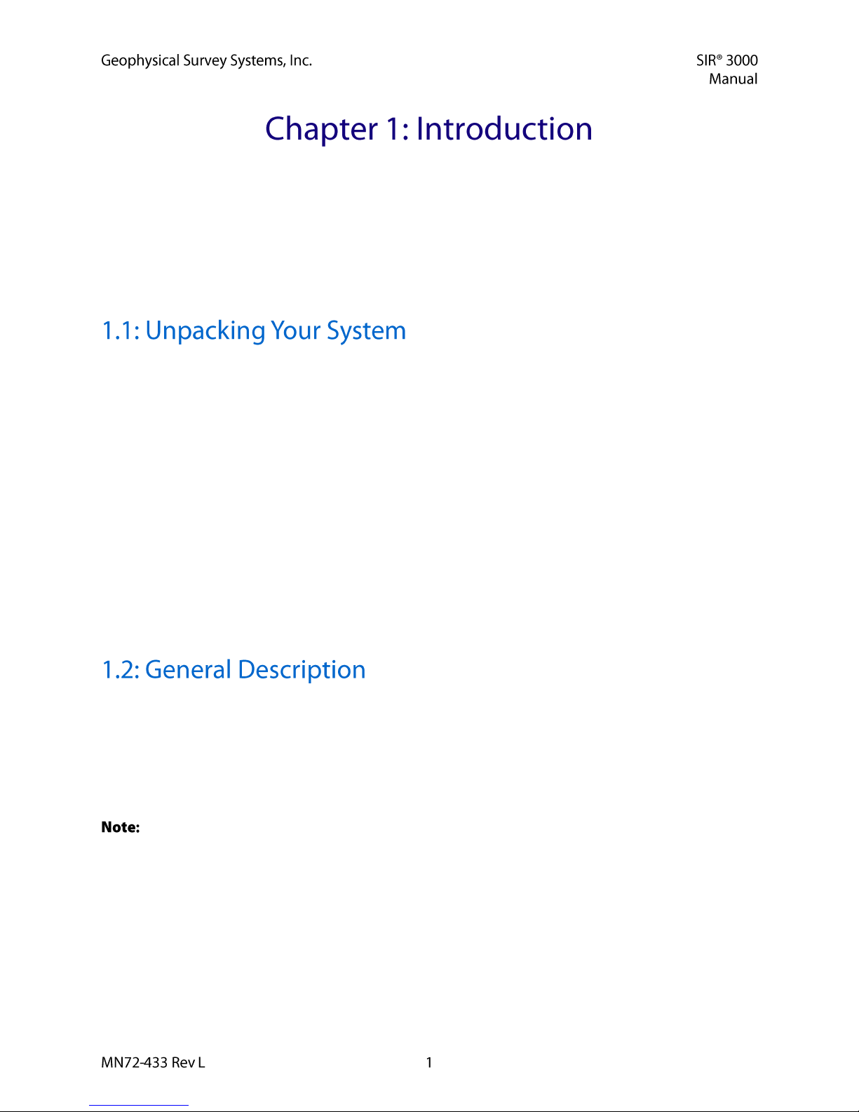
The major external features of the control unit are the keypad, color SVGA video screen, connector panel,
battery slot, and indicator lights. The video screen allows you to view data in real time or in playback
mode. It is readable in bright sunlight, although an optional sunshade for the unit is available. Prolonged
exposure to direct sunlight will cause the screen to heat up and may affect screen visibility.
Do not use Windex or other ammonia-based glass cleaner to clean the display screen as this may
damage the coating. Use only a clean, slightly damp cloth to gently clean the screen. Due to the screen’s
special coating for direct sun viewing, it is very susceptible to scratches. Take extreme care not to use any
abrasive materials or any solvents to clean the screen. The only recommended cleaning tool is a camera
quality lens cloth. Screen replacement due to scratching is not covered under the system’s warranty.
Page 8

The battery slot in the front of the unit accepts the 10.8 V Lithium-Ion rechargeable battery provided.
Survey time with a fully charged battery is approximately 3 hours. Batteries are recharged with the
optional battery charger or by simply leaving the battery in the unit and connecting the unit to a standard
AC source and leaving the system in standby mode. Time to recharge a battery is approximately
4-5 hours. Be sure to keep the battery slot cover on the unit while in use to ensure that no dust or dirt
enters the unit’s interior.
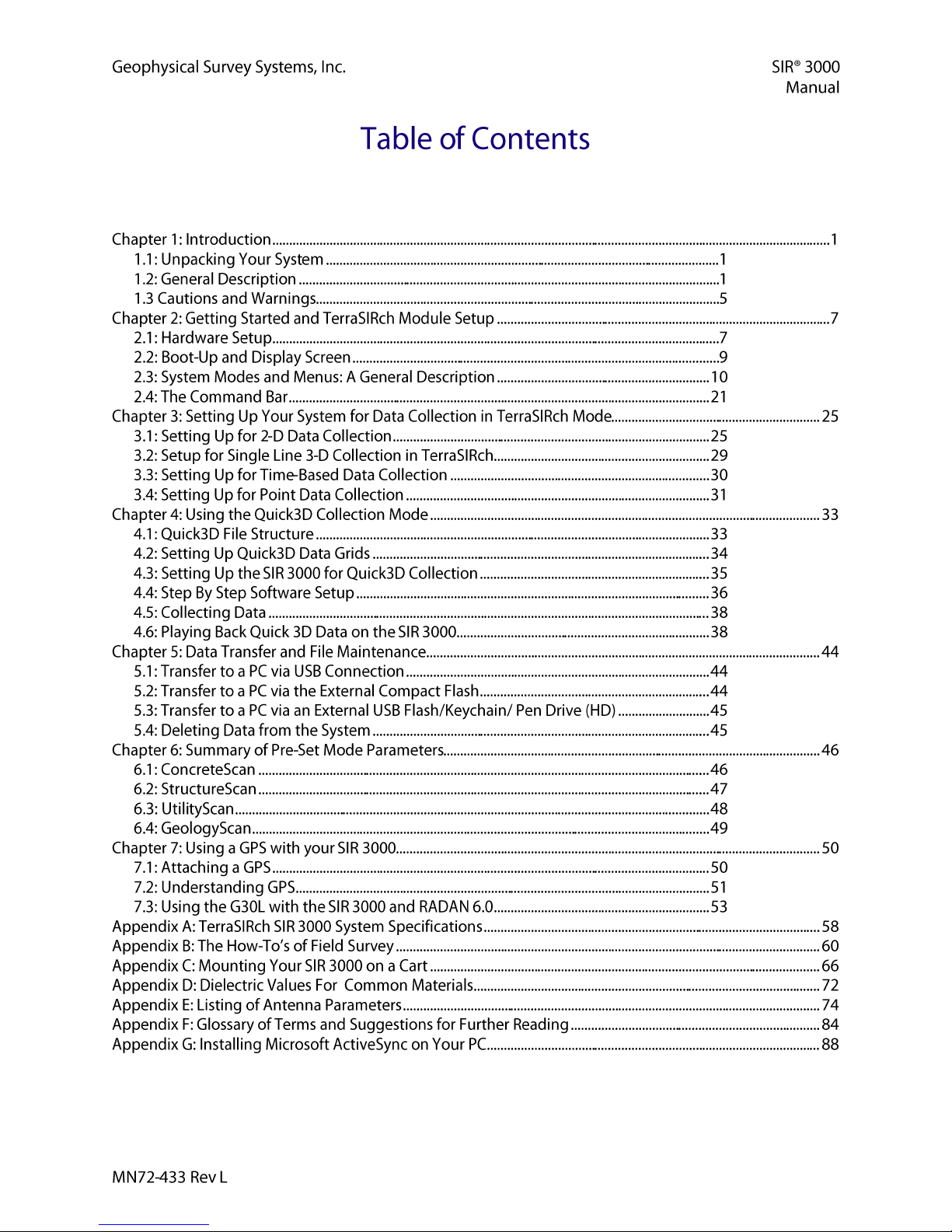
On the back edge of the unit, the SIR 3000 has six connectors and one slot for the memory card. The five
top-row connectors are, from left to right: AC Power, Serial I/O (RS232), Ethernet, USB-B, and USB-A.
Data can be stored on Compact Flash cards, USB key drives (Compact Flash format), or
IBM Microdrives for transfer to PC for processing. These cards are widely available and are the same
type used in other digital devices such as cameras, MP3 players, and camcorders. The amount of system
card memory is totally dependent on your choice of memory card size.
Since radar profiles can sometimes be several megabytes in size, GSSI recommends that you
purchase a high capacity card.
If there is no memory card inserted when the system is first turned on, the system will save the
data profile to its internal system memory and data will have to be transferred with the USB
connection or by later inserting a memory card. The internal memory capacity is approximately 1
gigabyte. Please see Chapter 4: Data Transfer and File Maintenance for additional information on
transfer.
The large, protruding 19-pin connector at the back of the system is for the antenna
control cable. You will notice that antenna connection on the SIR 3000 has five notches cut from the
metal. These mate with the five raised nubs on the control cable to ensure that the pins line up properly.
Screw the cable connector collar onto the SIR 3000 to make proper contact. The cable should
only be hand-tightened. Do not use a wrench to tighten the connection as over-tightening will
result in damage. The cable connector collar should be screwed down far enough to cover the red
line on the SIR 3000 connector.
The only proper time to attach or detach an antenna is with system power off. Be sure to unplug
any external power and to remove the battery before attaching or detaching antennas. Putting the
SIR 3000 in Sleep Mode is not sufficient.
: Use of a Model 3207 pair (100 MHz) or a Model 3200 Multiple Low Frequency antenna
without a TR fiber optic link will cause damage to the SIR 3000’s transmit circuitry. Always be sure to
use a Model 570 Fiber Optic Transmit Link with the Model 3207 pair and use the fiber optic transmit
cable for the 3200 MLF.
Page 9
Plug in the supplied universal AC power adaptor to run the system from 110-240 V, 47-63 Hz
power.
This is a standard serial connection that can be used to establish communication
between the SIR 3000 and a GPS. Please see Chapter 7: Using a GPS with your SIR 3000 for additional
information. This port is also used to connect the serial lead from the StructureScan Optical barcode
reader cart to the SIR 3000.
Functionality for this port is not currently available.
These ports are for connection to a variety of USB peripherals, including a keyboard
and memory device.
Page 10

The keypad on the front of the unit has fifteen (15) buttons and two indicator lights.
This button turns the SIR 3000 on and off. To start up the system, insert a battery or connect AC
power and push the power button.
This grouping of five buttons is located right below the power button. The Enter key
is the one in the center. These buttons allow you to navigate through the menu tree.
Highlighting a menu item by pushing Up or Down on the menu tree and then pushing the Right
arrow will open any menus that are under that menu choice. Left arrow will collapse those menu
items to refresh the menu tree.
Pushing the Enter key on some menu items will cause a pop-up menu to appear so you can toggle
between two or more parameter choices.
For example: To setup data collection mode, pushing Enter when COLLECT > RADAR > MODE is
highlighted will bring up a pop-up menu which will allow you to choose from Time (continuous data
collect), Distance (survey wheel), or Point measurement. Highlight your choice and push Enter to see
your choice applied, and then Right arrow to accept and cause the pop-up menu to disappear.
This button is located below the Enter/Arrow Pad. Pushing this button while collecting data
will cause the system to set a User mark in the data.
User marks are helpful for noting distance traveled if you are not using a survey wheel and for
noting the location of obstacles such as columns, trees, pits, etc.
User marks will appear as long, dashed, vertical white lines through the data window.
This button is located below the Insert Mark button. Pushing the Run/Stop button in
COLLECT > RUN stops data collection and brings up a set of crosshairs. Clicking this button again
closes a data collection file and causes the system to ask if you want to save that file. Clicking this button
during Setup in modes other than TerraSIRch or Quick 3D will cause the system to re-initialize the gain
and position servos. This will reset the gains to the area under the antenna and could minimize clipping.
This button is located under the Start/Stop button. Pushing the Help button will bring up a menu of
help topics. The onscreen help is only accessible from the TerraSIRch splash screen. Use the Mark
button to highlight links and Enter to jump to a help topic. Pushing the Run/Stop button on the right hand
side of the unit will take you back to the previously viewed screen.
These six (6) buttons are located below the video screen. Pushing one of these from the
initial start screen will cause the SIR 3000 to operate in the desired software module.
Page 11

Do not use Windex or other ammonia-based glass cleaner to clean the display
screen as this may damage the glare reduction coating. Use only a clean, slightly damp cloth to gently
clean the screen. Due to the screen’s special coating for direct sun viewing, it is very susceptible to
scratches. Take extreme care not to use any abrasive materials or any solvents to clean the screen. The
only recommended cleaning tool is a camera quality lens cloth. Screen replacement due to scratching
is not covered under the system’s warranty
Antennas are not hot-swappable. You
must turn off the SIR 3000 before connecting or disconnecting an antenna. Failure to remove power
may cause damage to the SIR 3000.
The SIR 3000 is weather resistant, but not weather proof. Try to avoid getting
the system wet. If you believe that water has gotten inside of the system, disconnect power, open the
battery compartment and input connector compartment on the back and allow the system to
thoroughly dry.
Use of a Model 3207 pair (100 MHz) or a Model 3200
Multiple Low Frequency antenna without a TR fiber optic link will cause damage to the SIR 3000’s
transmit circuitry. Always be sure to use a Model 570 Fiber Optic Transmit Link with the Model
3207 pair and use the fiber optic transmit cable for the 3200 MLF.
Page 12

Page 13

In Chapter 2, you will find instructions for connecting all of the hardware inputs and an introduction to
the different menus and functions that are available to you in TerraSIRch mode. TerraSIRch mode allows
you total control over all collection parameters and is the most versatile data collection method, usable for
all GPR applications. If desired, these 2-D profiles can later be transferred to a PC for processing in
GSSI’s RADAN™ post-processing software.
Hardware setup for the SIR 3000 is very simple. We will assume the 400 MHz (Model 5103) antenna for
this example, but the hardware connections are the same for other GSSI antennas, and the cable
connections are clearly marked. Follow the steps below.
Attach the survey handle between the two vertical mounting plates on the top of the antenna with the
two removable pins, adjust the angle for comfort, and connect the marker cable to the antenna at the
MARK port.
Page 14
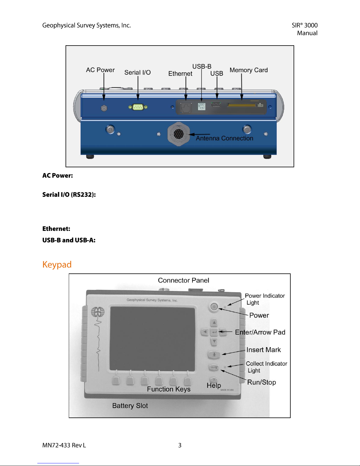
Connect the female end of the antenna control cable to your antenna. Then connect the male end to
the antenna connection on the back of the SIR 3000. Connect the two protective caps together. Attach
the survey wheel to the brackets at the back of the antenna (as shown below) and connect the cable to
the SURVEY port on the top of the antenna. Be sure that the triangular plate protecting the survey
wheel encoder faces down.
Connect power source (battery or AC) to the SIR 3000 and push the power button to turn on the
system.
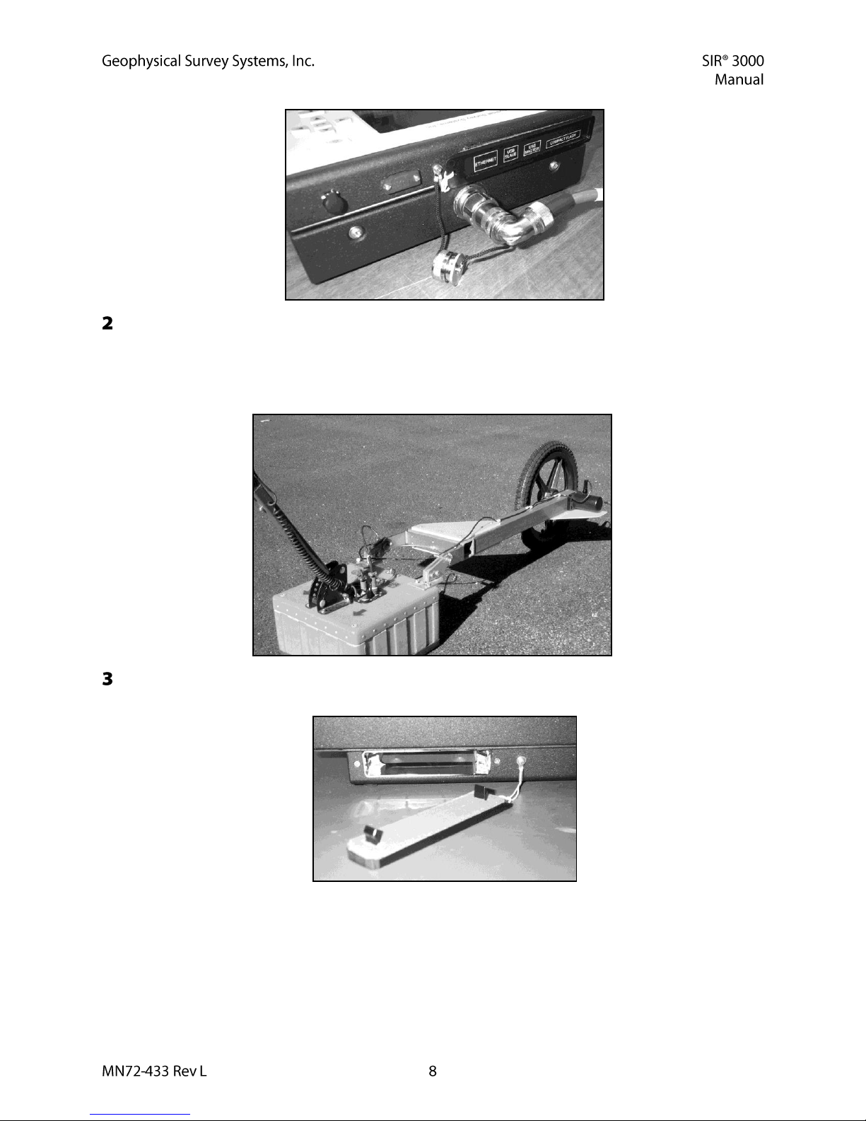
If you purchased your SIR 3000 with a cart as in the UtilityScan System, or purchased the cart system
separately, please see Appendix C: Mounting your SIR 3000 on a Cart. The cart also incorporates a
survey wheel that is used in place of the survey wheel pictured earlier. If you have a StructureScan™
Standard or StructureScan™ Optical system, please consult the hardware setup instructions in the small,
laminated QuickStart Guides that came with the system.
Page 15
After the SIR 3000 boots up, you will see the introductory screen. There will be 6 icons positioned over
the Function Keys. The first one is TerraSIRch.
Pushing the Mark button switches your desired units between English and Metric.
TerraSIRch mode gives you complete control over all data collection parameters. Quick Start guides are
available for StructureScan and UtilityScan. The StructureScan Quick Start guide also covers the
ConcreteScan functionality. Push the TerraSIRch button. After a moment, you will see a screen divided
into three windows and there will be a bar running across the bottom with commands above each of the 6
Function Keys.
After entering one of the six data collection modes, you can return to this screen by either clicking the
Power button twice or by removing the battery and AC power and reinserting it to re-boot.
For information on other modes, please see Chapter 6.
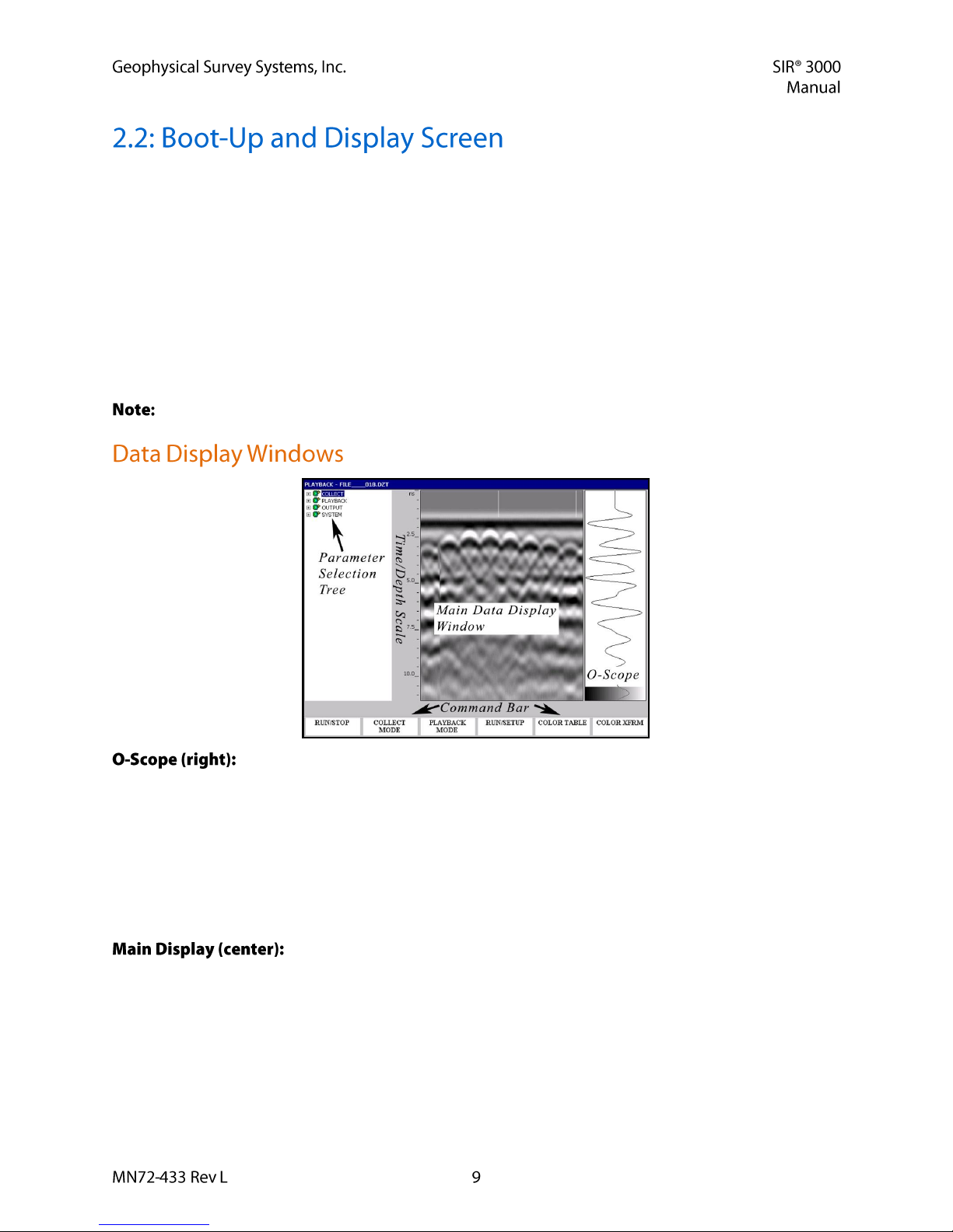
On the far right of the screen you will see a window that shows a single radar scan in
an oscilloscope-style (O-scope) depiction. This will show successive single scans as you move your
antenna across an area while in Setup mode.
Time (depth) increases down the screen.
At the bottom of the window you will see a color bar. This shows you the distribution of colors
across the range of reflection amplitudes (size of the peaks of the scan to the left and the right of
center). The exact color and distribution depends on your choice of color table and color
transform.
The main data display window in the center shows a radar profile in linescan
format. In this depiction, successive single scans are assigned color values and stacked next to each other
in sequence to form a continuous image.
The vertical scale on the left of this data display window shows time, depth, or sample number.
New scans will be placed at the right side of the window and data will scroll from right to left.
Page 16
The bar across the bottom of the screen is the Command bar and allows you
different toggles and functions depending on whichever system mode you are in at the time. You can
activate these commands by pushing the function key right below the wording. These commands are each
explained in more detail later on when the different system modes are discussed.
To the left of the main data display window is the parameter selection tree
window. This window is where you will navigate through the various commands, set system parameters,
and enter file name information. The tree is similar to the basic folder and file browser seen in many
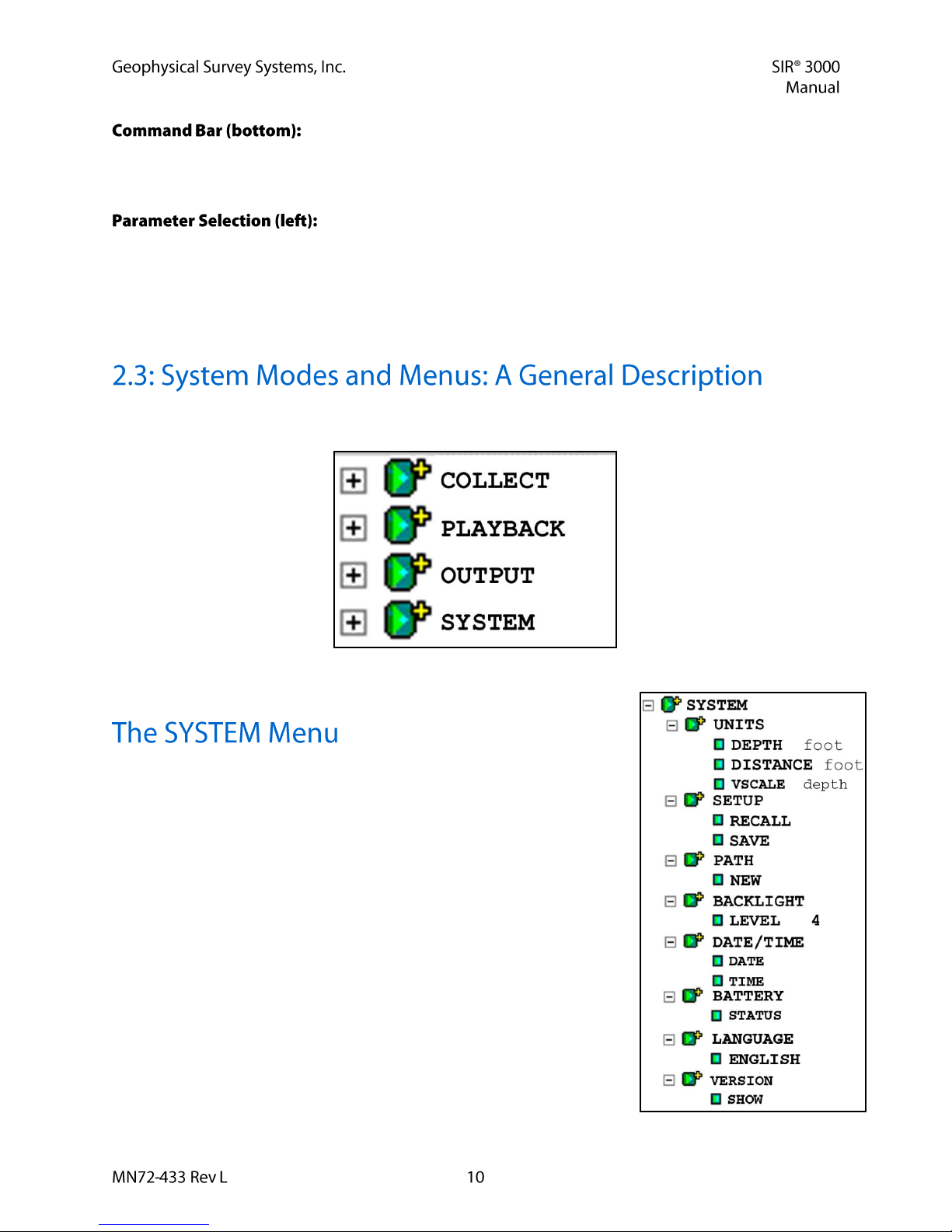
Windows-based applications. Upon setup, you will see three choices that indicate the three modes of the
SIR 3000, COLLECT, PLAYBACK, and OUTPUT, as well as the SYSTEM menu used to change
system parameters.
The SIR 3000 has four main system menus, Collect, Playback, Output, and System. We will first look
briefly at the System menu.
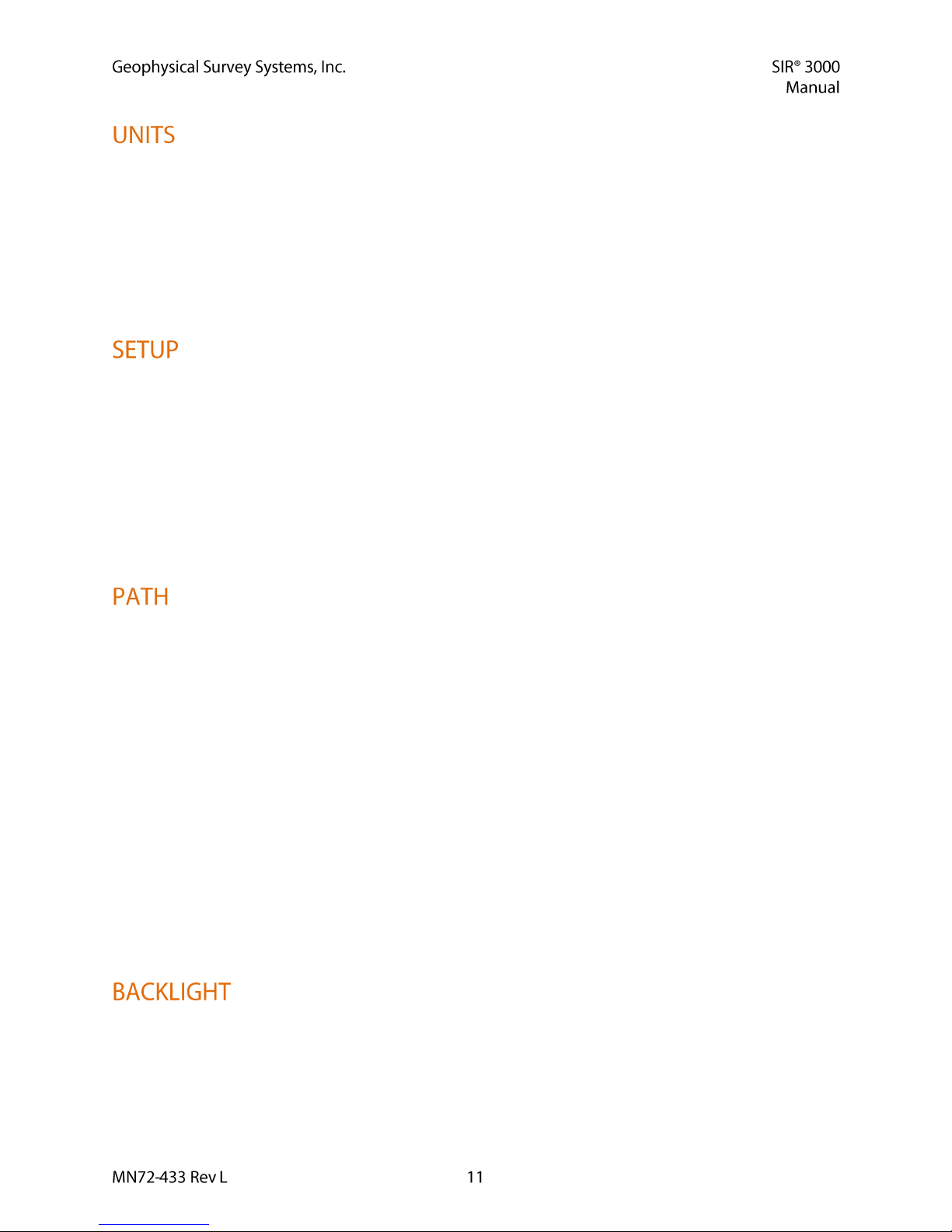
If you are using your SIR 3000 for the first time or if you need to change
some system parameters, you should enter this menu first. Highlighting
SYSTEM and pushing the Right arrow will bring out seven additional
menu choices:
UNITS (page 11)
SETUP (page 11)
PATH (page 11)
BACKLIGHT (page 11)
DATE/TIME (page 12)
BATTERY (page 12)
LANGUAGE (page 12)
VERSION (page 12)
Page 17
You can select appropriate units for DEPTH and DISTANCE, as well as the appropriate scale. For
example, if you are using a very high frequency antenna to scan 18 inches into concrete, you may choose
to display depth in inches and distance in feet. Under VSCALE, you can choose to display in depth, time,
or height. Time is measured in units of nanoseconds (ns). When set to time, the vertical scale displays two
way travel time (TWTT). If you set to depth, then the SIR 3000 will perform a time to depth conversion
based on the dielectric value that you have set in COLLECT > SCAN. It will then display the vertical
scale in depth. Height will invert the screen so that time-zero is at the bottom. This can be a useful display
if you are scanning upside-down.
This allows you to either save the current list of data collection parameters (hereafter called a setup),
recall saved setup, or a factory loaded one.
Factory setups cannot be overwritten, but the system has 16 slots where single user setups can be
saved.
After choosing your antenna under the COLLECT mode, you will have to find the correct setup
for that antenna and recall it.
These are named SETUP01 to SETUP16. SETUP00 is a default setup that contains the
parameters the system was collecting the last time that it was used.
Think of this as the location in which your files are stored on the SIR 3000. There are two basic types of
paths: Common and User-defined.
Each file in the Common path will be named with the word FILE and then a number. For
example, the first data file will be FILE001, then FILE002, and so on.
The user-defined path allows you to change the root name (instead of FILE) and the location of
your data. This is useful if you are surveying multiple areas or if you prefer to name your files
during collection with a site name instead of doing it later after download.
To create a user-defined path, select NEW from the Path menu. This will bring up a window with
six letters and an Up/Down arrow. Enter the new name by scrolling through the letters with the
Up/Down arrow. You can advance to the next ‘digit’ by using the Enter button. Once you are
finished, click the Right arrow.
To delete a Path you must first delete all of the data files. Then select TRANSFER > DELETE
again, the Remove Files window will pop-up, and you will see an option to REMOVE PATH.
Click Enter to put a check in that box and then Right Arrow to accept. The path will be removed
and the system will default to the Common path.
This controls screen brightness. The scale runs from 1 to 4 with 4 being the brightest. The darker the
screen is, the longer the battery will last because powering the screen is a large draw on the power supply.
Page 18

Use this selection to set the system’s internal clock to the current date and local time. The SIR 3000 will
attach this information to each radar profile you collect. This information is saved and will not be lost
each time you turn the system off or remove the battery.
This selection allows you to check the remaining charge on the battery. The value here is rough
estimation of the remaining time until the battery is too low to power the SIR 3000. If you have external
power connected, the window will say External Power Supply.
This allows you to change the display language of the SIR 3000 to a number of pre-loaded language
packs. If your native language is not available, check the GSSI website periodically to see if the language
patch is available for download.
This allows you to check the current version of the TerraSIRch operating software. You should check the
GSSI website for updates to the Graphical User Interface (GUI) software. The GUI is listed at the bottom
of the Version pop-up window. Note which GUI version you have, then go to the GSSI Technical Support
website at , and click on the SIR 3000 Updates tab. You should also
download the instructions for the download. You will need a USB cable to link your SIR 3000 to your
PC, and you will also need a password and username for the secure section of GSSI’s website. You may
register for a password on the Technical Support section of the website.
Page 19
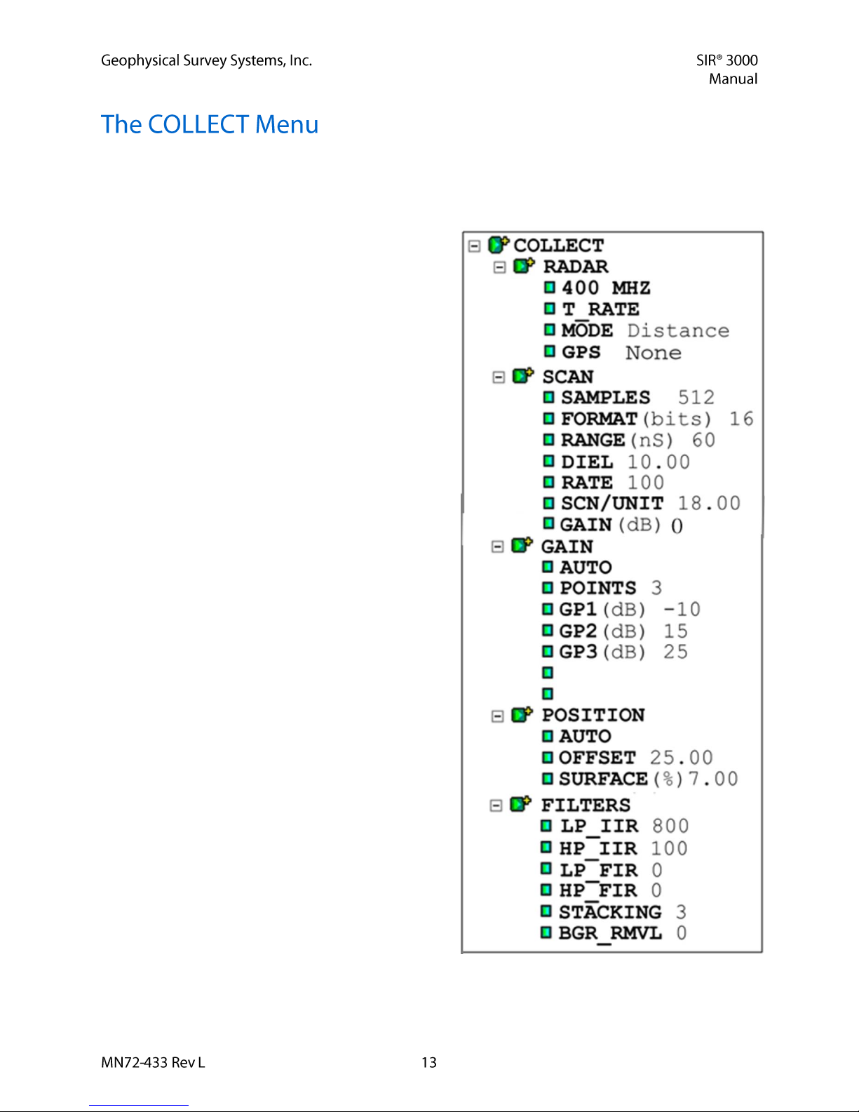
The COLLECT menu is similar to the Collect Setup mode on the older GSSI SIR 2 and SIR 2000. If you
are familiar with those systems, you will notice a lot of similarities here. Under COLLECT, there are five
main sub-menus that can each be accessed by pushing the Down arrow to highlight the sub-menu, then
the Right arrow to see additional menus inside the sub-menu. These are:
SCAN (page 14)
GAIN (page 16)
POSITION (page 17)
FILTERS (page 17)
Page 20
This sub-menu has four main choices: Antenna, T_RATE, MODE, and GPS.
Under this menu, you will be able to enter the center frequency of the particular
antenna you are using. This will allow the SIR 3000 to perform the auto-surface operation.
The T_RATE is the antenna transmit rate in KHz. This rate is capped at 100 KHz. A higher
transmit rate equals faster data collection ability. Some older antennas however, are not capable of
transmitting at high speeds and setting them at a high transmit rate may cause error. Please consult your
antenna documentation or call GSSI Tech Support if you have any question about transmit rate. All GSSI
5100 and 52000 series antennas (2.6 GHz, 2.0 GHz Palm, 1.6 GHz, 1.5 GHz, 1.0 GHz, 400 MHz, 270
MHz, 200 MHz) can be driven at 100 KHz. If you are using another GSSI antenna, consult Appendix E
for the proper transmit rate.
If your SIR 3000 beeps repeatedly with an older/high power antenna, you may have your T_RATE
set too high. This beeping is a high-voltage overload warning. A prolonged overload could damage your
system. Lower your T_RATE until the beeping stops.
The MODE selection allows you to collect data as point, distance, or time based. Point data
collection is commonly selected only for very deep applications or very difficult terrain. The system will
record one scan every time the external marker or Run/Stop button is pressed. The antenna is then moved
to the next location and the next scan is taken. In time based data collection, the system is recording a
certain amount of scans per second. The data density over an area depends on the speed that the antenna is
moved over the ground. The rate (scans/second) is set in the SCAN submenu. Distance-based collection is
performed with a survey wheel. The system records a certain number of scans per unit of distance. This is
the most accurate data collection method and it is strongly recommended that you collect data in this
mode if possible. Distance-based data is required for 3D files
This selection allows you to toggle the GPS capability on and off. Connect the GPS to the serial
port, and toggle this either to G30L if you are using the GPS receiver obtained from GSSI, or to
CUSTOM if you are using another GPS receiver.
If you are using the Acumen SDR Data Bridge/Logger purchased from GSSI, attach the serial lead from
the GPS to the Data port and attach the lead from the SIR 3000 to the Config port, and then select SDR
from the list under RADAR > GPS.
Consult Chapter 7 of this manual for additional instructions and setting up the GPS and working with it.
GSSI publishes information about GPS integration as Technical Notes that are available on the GSSI
Technical Support website at .
Scan contains six additional menus: SAMPLES, FORMAT, RANGE, DIEL, RATE, and SCN/UNIT.
Each scan curve is made up of a set number of individual data points, called Samples. The
more samples you collect, the smoother the scan curve and the better your vertical resolution will be.
You can choose from a preset list of 256, 512, 1024, 2048, 4096, or 8192 samples per scan. FIR
filters should not be used with 4096 or 8192 samples per scan.
Note that as sample number increases, maximum scan rate drops and file size increases.
GSSI recommends sampling at 512 or 1024 samples per scan for most applications. More
samples will be required for deep geologic or polar ice thickness applications.
Page 21

Data can be collected in either 8-bit or 16-bit format. 16-bit data is recommended for most
applications because it has a greater dynamic range, meaning there is more information in the data. If you
are only collecting data to be viewed on the screen (no processing), or are collecting very high
samples/scan data, you should set this to 8-bit data. 16-bit data profiles are twice as large in terms of
computer storage.
RANGE is the time window in nanoseconds (ns) that the SIR 3000 will record reflections. The
time range is proportional to depth viewed because a longer range will allow more time for energy to
penetrate deeper and give reflections from deeper down.
It is important to remember that the range is two-way travel time, so that a range of 50 ns means
that the deepest reflector is 25 ns deep.
Bear in mind that you still have a set number of samples to draw a curve and a very long range
may require a greater number of samples. The range can be set from 5-8000 ns.
Please see Appendix B for a list of common ranges for individual antennas.
DIEL refers to the dielectric constant of a material. Basically it reflects the velocity that radar
energy moves through a material.
If you know the dielectric value of the material that you are surveying through, you can enter it
here and get an in-field time to depth calculation.
Higher dielectric values mean slower travel time and shallower penetration.
Generally speaking, water raises a material’s dielectric constant, and surveys should be performed
on dry material whenever possible.
Please see Appendix D for a chart of dielectric values of common materials and a deeper
discussion of dielectrics. Possible values are 1-81.
Example: In air, which has a dielectric constant of 1, radar energy will travel at 12 inches per ns. Since
the time range is two-way travel time, 1 ns on the vertical scale translates to 6 inches if the DIEL is set to
1. The distance traveled per ns is reduced by the square root of the dielectric constant. The dielectric
constant of water is 81, so that water slows down the radar wave by a factor of 9 (√81=9). The range in
water is thus 6/9 inches per ns.
The next selection is scan RATE. This value is the number of scans the system will record in its
RAM memory per second.
If you are collecting data based on time, this is the number of scans that will be saved each
second.
If you are collecting data based on distance with a survey wheel, this number should be set very
high.
If you tell the system that you want to collect 60 scans a foot, and you move more than one foot per
second, the system is going to look for scans which aren’t available. This is called dropping a scan.
Assuming your T_RATE is 100 KHz, this setting should be at 120 whenever you are collecting with a
survey wheel and are collecting a max of 512 samp/scan.
If you set this value higher than possible given the 100 KHz T_RATE and the number of samples/scan,
the SIR 3000 will automatically lower it to the maximum possible.
Page 22
The last choice is SCN/UNIT, or scans per unit of horizontal distance. This parameter is the
scan spacing when you are collecting with the survey wheel.
Having a smaller scan spacing produces higher resolution data, but larger file sizes. The number
here is the number of scans that the system will collect per unit of distance. So for example, if
you see a 12 here and the system is set to English feet, rather than Metric units, you will collect
12 scans per foot, or 1 per inch.
The StructureScan setting for shallow structural features in concrete is 60 scans/foot or
5 scans/inch. The StructureScan setting also allows you to set to 7.5 and 10 scans/inch. Ten per
inch is the densest recommended scan spacing, and it is only meant for the 1.5/1.6 GHz, 2.0 GHz
Palm and the 2.6 GHz antennas.
Lower frequency antennas, like the 400 MHz will require coarser scan densities
(12-24 scans/foot).
This value is for display purposes. It will apply a display gain to the data that may make the data
easier to view while collecting. This will not be saved with the data file.
Gain is the artificial addition of signal in order to counteract the natural effects of attenuation. As a radar
scan travels into the ground, some of the scan is reflected, some of it is absorbed, and some of it keeps
traveling down. As the scan gets deeper, it becomes weaker. We apply gain to the scan to make the subtle
variations in weaker data more visible. The two choices under the gain menu are a MANUAL/AUTO
toggle and a listing of point numbers.
Setting the GAIN to MANUAL will allow you to change the number of gain points and to add
strength to the signal at your own discretion. This is not recommended for inexperienced users as
it is possible to ‘create’ features in the data by over-gaining areas.
Setting the gain back to Auto will cause the system to re-initialize and adjust its gains to the area
under the antenna. This is useful if you find that your data is clipped (over-gained) over a
particular section of your survey area. Just place the antenna on the area where the data is clipped
area and toggle the gain to Manual, and then back to Auto. This will cause the system to reset the
gains to a lower level, and prevent clipping.
Gain is applied at a number of evenly spaced points throughout the data scan. You can select up
to 5 gain points, and then manually add or subtract gain values from individual points.
The gain curve is visually represented by a red line in the O-Scope window on the Setup screen.
Values increase from left to right and the location of gain points is shown by a change in the
slope of the curve.
Use caution not to add too much gain to a single point because you may create what will look like
a layer in the data. The software will automatically adjust lower gain points to be equal to or
greater than higher points. This is done to avoid a negative gain slope.
The SIR 3000 is only displaying about 25% of the amplitude range. This means that even if your
data appears slightly clipped, the SIR 3000 is likely still recording the full amplitude range of the
reflection. If you use a –12 dB display gain, you will see an accurate representation of the recorded scan.
This also means that when you view your data in RADAN, it will appear under-gained and you will need
to add some display gain.
Page 23

This menu controls the position of Time-Zero. Time-Zero is the location of the beginning of the time
range, and thus the beginning of the scan. Typically, having the system auto locate itself is enough to
adequately set the position. If however, you need to manually adjust the location of Time-Zero, this is the
place to do it. Position contains three additional menus: MANUAL/AUTO, OFFSET, and SURFACE.
The MANUAL/AUTO toggle will allow you to make adjustments in manual mode
and cause the system to re-servo (just like in the gain menu) when switched back to auto. GSSI
recommends that inexperienced users keep the position set to Auto. This choice is automatically set to
MANUAL if you are using sample densities of 4098 or 8192.
This is an internal system parameter that describes the time lag (in ns) from the SIR 3000
triggering the pulse inside of the control unit until we consider it to have transmitted from the antenna
itself. Since there is no way to accurately measure the exact moment the pulse leaves the antenna, we use
the antenna’s direct coupling to figure out the appropriate point to set the offset (and thus the transmit
pulse). The direct coupling is the pulse that travels inside of the antenna housing, directly from the
transmitter to the receiver, and it is generally considered to be the first response in the data.
As long as the antenna dipoles are not very far apart, as is the case with a separated bistatic antenna pair,
the direct coupling happens before any reflections from the ground. So if we make sure that we have the
direct coupling visible in the data, we can be sure that we have 100% of our data and most importantly,
the ground surface to perform a depth calculation. The number here is nanoseconds from trigger pulse
inside the SIR 3000. If you need to adjust this parameter, use caution not to lose that direct coupling
wave.
SURFACE, is a useful display
option and is new to the SIR 3000. This
allows you to visually ‘cut out’ the flat part
of the scan and the direct wave, and show
the scan from the first reflected target,
which should be the ground surface. The
other information is still collected and
saved, but not displayed. This allows you
to set the display to show an in-field time
to depth calculation. For simplicity, the
value is set as a percentage of the total
vertical window. The SIR 3000 will
examine the offset and the antenna type
you entered under RADAR to find the
proper surface automatically. It will set
near to the first positive peak of the direct coupling. In the image at the right, the antenna was moved up
and down over the ground surface. Notice how the surface reflection moves up to join the direct wave.
This menu allows you to set data collection filters to either remove interference or smooth noise. Many of
these are antenna-specific, especially the High and Low Pass filters. In ConcreteScan, StructureScan,
UtilityScan, and GeologyScan, these will be automatically set when you choose your antenna under the
RADAR menu. In order to set factory values for the filters you must recall a factory setup for the
antenna you are using under SYSTEM > SETUP > RECALL. There are six menu selections here:
Page 24

LP_IIR
HP_IIR
LP_FIR
HP_FIR
STACKING
BGR_REMOVAL
The first four are frequency filters and the values are all expressed in
MHz.
The two types of filters that we are using are the Finite Impulse Response (FIR), and Infinite Impulse
Response (IIR). We are using these to downplay external interference, and thus clean up the signal. The
FIR filter does this without altering the phase of the signal. For some antennas we also use a very low IIR
filter to clean certain characteristics of that antenna’s signal. These filters are antenna-specific and are set
automatically when you recall the proper setup for your antenna.
FIR filters should not be used with 4096 or 8192 samples per scan.
LP stands for low-pass, which means that any frequency lower than the one entered here will be
allowed to pass by and be recorded by the system.
HP stands for high pass, which means that any frequency higher than the one entered here will be
allowed to pass by and be recorded by the system.
By setting these at different ends of the antenna’s bandwidth, you are determining the range of
frequencies that the antenna is filtering out.
The default values will be adequate in almost all situations.
After the frequency filters, the next choice is Stacking. Stacking is a high-frequency noise
reduction technique. It is an IIR filter which operates in the horizontal direction. Each new scan has a 1/n
influence in the data, so this filter has a tendency to smooth high frequency targets and accentuate low
frequency horizontal features, such as layers. As the number of scans you stack (n) increases, the
influence of each new scan drops. If you put in a very high number, you will filter out high frequency
targets in your data. This might lead to missing real targets in your data.
High frequency noise generally has a ‘snowy’ appearance.
The larger the number you put in here, the smoother the data will be. It is possible to over smooth
and ‘smudge’ out real data.
A larger number also means that the system is performing a great deal of extra calculations and
data collection speed will then be reduced.
The Background Removal filter is a horizontal high pass (remove low frequency
noise) operation meant to remove flat-lying noise associated with antenna ringing.
The input number here is scans, so in order to use this filter, find the length in scans of the feature that
you want to remove and put that number into the system. Features of this size or larger will be removed
from the data.
Also please note that this filter will remove your direct coupling, making positive identification of
Time Zero difficult. To preserve data integrity it is best to collect data without this filter and then
apply it in playback or post-processing if needed.
Page 25
If you want to review the data you just collected or access any of the Playback functions, push the Down
arrow to highlight the particular menu choice.
If you would like to review a previously collected file, pushing the Playback function key will bring up a
window that lists stored data files.
If you select a single file, it will cycle through that one, or you can choose multiple files and the system
will play them back in sequence.
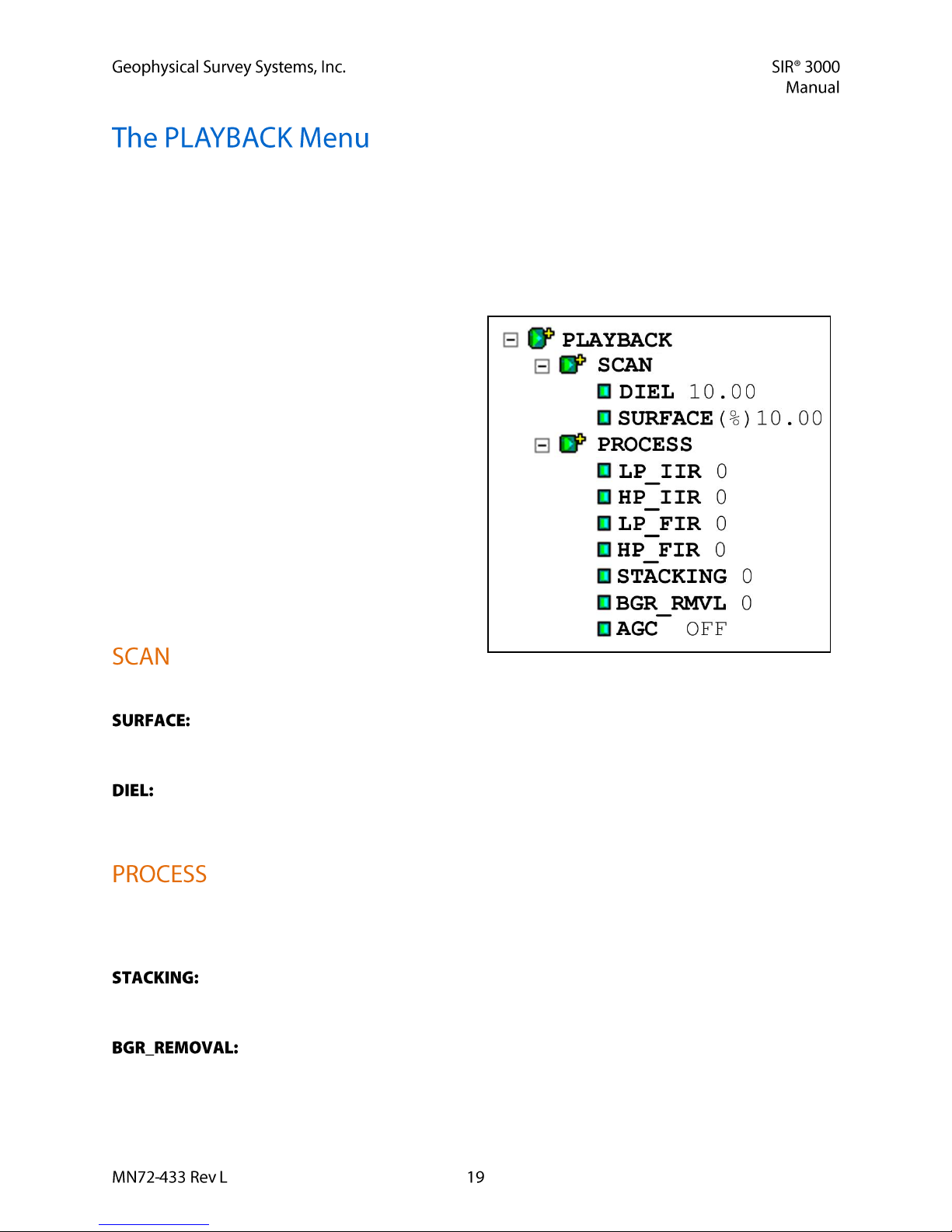
The playback menu has two sub-menus:
SCAN (page 19)
PROCESS (page 19)
The scan sub-menu contains two parameters: DIEL, and SURFACE.
Surface operates just like the surface item in the Position sub-menu of Collect menu, and it
has been duplicated here for convenience. Once again, this input is percentage based. Changing the
surface position here will not permanently eliminate any data.
The Diel parameter allows you to input the dielectric constant so that the system can do a time to
depth calculation. Once again, for convenience, this parameter is duplicated from the Scan sub-menu of
the Collect menu. Possible values are 1-81.
This menu allows you to apply different filters and mathematical operations to the data in order to remove
noise or make subtle features more visible. These functions do not permanently alter the data, but are only
for display purposes.
Stacking in Playback Mode differs from the Stacking function in Collect Mode. The
Playback Stacking is also a horizontal, high-frequency noise reduction technique, but here it is an FIR
filter with a boxcar shape.
The Background Removal filter is a horizontal high pass (removes low frequency
noise) operation meant to remove flat-lying noise associated with antenna ringing.
Page 26
The input number here is scans, so in order to use this filter, find the length in scans of the feature that
you want to remove and put that number into the system. Features of this size or larger will be removed
from the data.
AGC stands for Automatic Gain Control. AGC lets you choose a set number of gain points (2, 3, or
5) distributed evenly through the vertical scale. The object of AGC is to normalize (make even-looking)
the scan by reducing the gain for areas where the signal is very strong (usually near the surface), but
adding gain with increasing attenuation (usually with depth). This dramatically slows the scroll speed of
the data, especially if 5 points are used. A faster option is Display Gain, located under the Display submenu in Output.
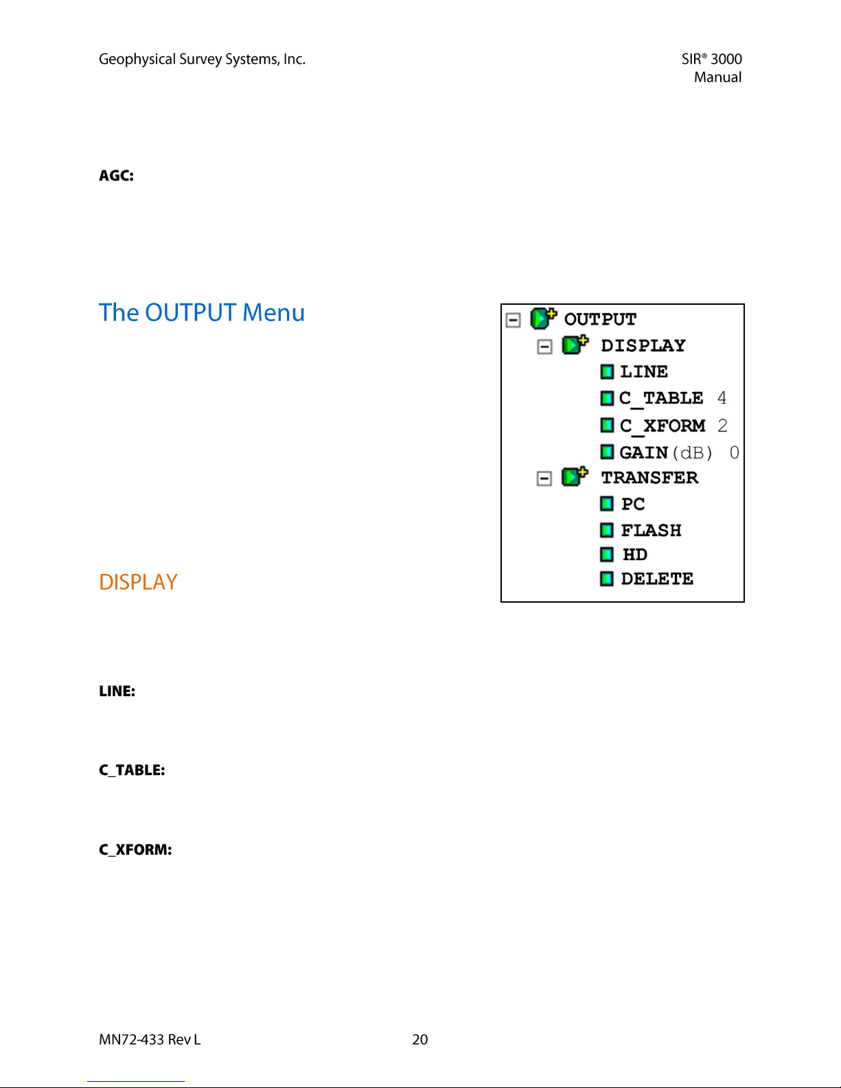
This menu controls the data display, printing, and file
maintenance. There are two sub-menus to the Output menu:
DISPLAY (page 20)
TRANSFER (page 21)
This sub-menu controls the ‘look and feel’ of the data
displayed on the screen. Here is where you can change the mode of display, color table and distribution
(transform), and add screen gain. There are four parameter inputs here: Mode (LINE/SCOPE),
C_TABLE, C_XFORM, and GAIN(dB).
This is really the Mode option which allows you to toggle between Linescan and Scope display
modes. Linescan is the conventional way of looking at GPR data with each scan stacked next to its
neighbor and amplitude values along that scan assigned a color value. Scope, or oscilloscope, mode
shows you the waveform of the individual scan.
This option lets you choose which of the pre-loaded color tables to use to view your data. In
addition to grayscale, there are several full color tables. It is sometimes useful to examine your data in a
number of different palettes because altering the colors may help you to see different aspects of your data.
There are 5 tables to choose from.
Once you have the data displayed in the proper color table, you may alter the distribution of
color shades across your data by changing the color transform under the C_XFORM option. This will
spread out your color shades over different sections of the scan’s amplitude range. You would do this to
show more color shades over the extremes or the mid-range values, or just a simple black to white.
Stretching more colors over a particular value ranges allows you to see more subtle variations in the data.
Bear in mind that not every transform is available for every color table. There are up to 4 different
transforms available.
Page 27
: The final display option is GAIN. This is often referred to as display gain, because it basically just
increases the amplitude of your data by multiplying every sample throughout your scan by a constant
value. The result is that you will be able to better see weaker reflections, but those already strong
reflections will be over-gained. This function is useful for a quick viewing of data that is attenuated or
otherwise under-gained to guarantee that it was not clipped.
This sub-menu allows you to perform file maintenance. The four options for this sub-menu are: PC,
FLASH, HD (hard drive), and DELETE. PC, HD, and FLASH allow you to move data from the internal
system memory to an external device, such as a PC, flash card, Microdrive, or an external USB keychain
drive. Transfer to a PC will be controlled by the external computer through Microsoft ActiveSync, while
transfer to the removable Flash card can be done using the SIR 3000’s buttons. For detailed instructions
on data transfer, please see Chapter 5: Data Transfer and File Maintenance.
The six keys across the bottom of the data display window have different functions depending on whether
you are in Setup (3 display windows) mode or in Run (1 display window) mode.
You are in Setup mode if you can see 3 display windows with the parameter selection tree at the left. If
you only see a single data screen (and no parameter selection tree), you are in Run mode.
***You can only collect data in Run mode. ***
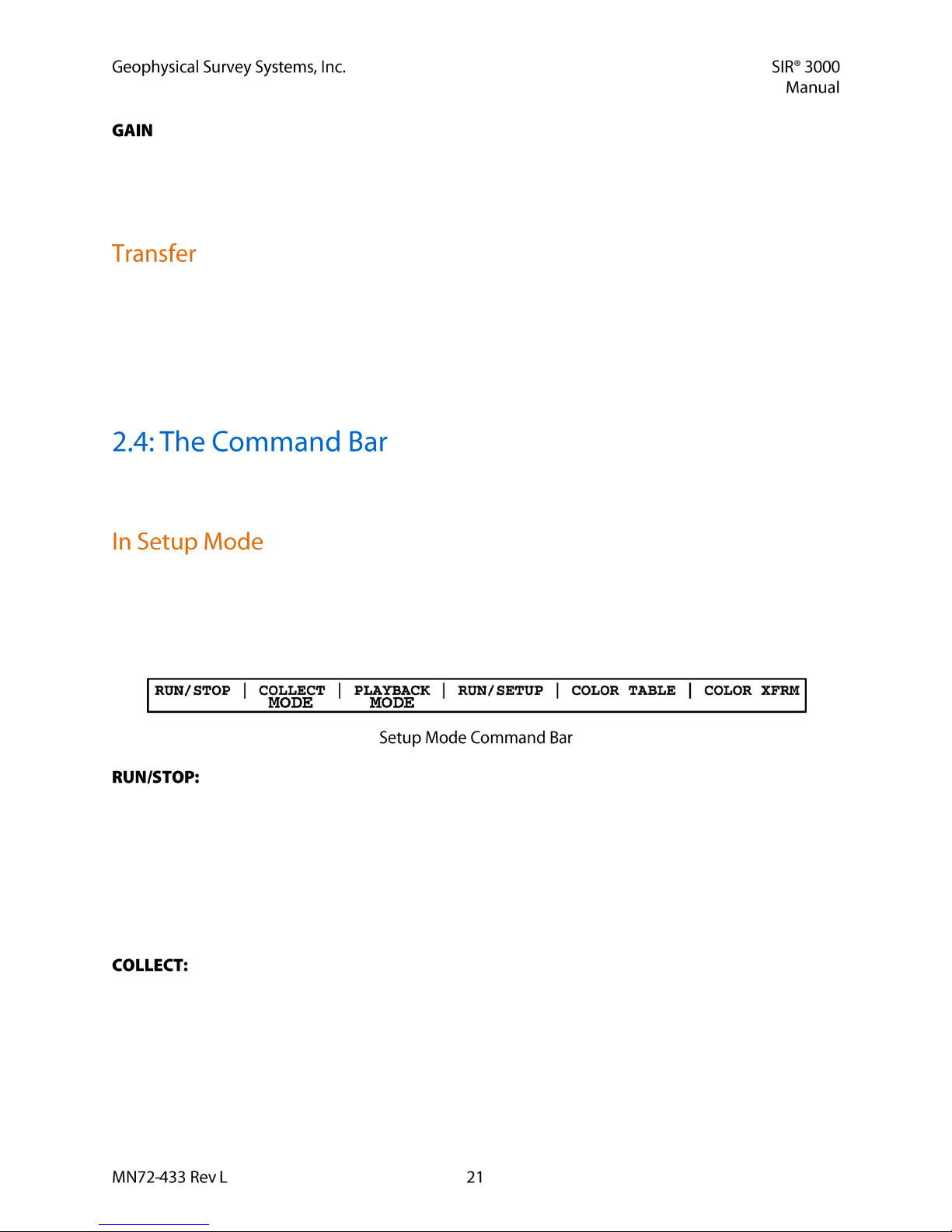
In Setup mode, the Command Bar will look like this:
This button stops the transmitter. The green light to the right of the Run/Stop button will
turn off. If you are in Setup mode (3 display windows), this will stop data from continuously scrolling
across the screen. If you are in RUN mode (a single display window), this will stop the data collection
and bring up crosshairs. You can then use the arrow keys to move the crosshairs over your data. You will
see two sets of numbers at the bottom-right of the screen. These give the location of the crosshairs. The
first number is the distance from the beginning of the profile, and the second is depth. Pushing this button
again will bring up the Save File window. After selecting YES or NO, you will automatically begin
collecting the next profile. The Run/Stop button under the marker button on the right hand side of the
system has the same function as this key.
This button has three main functions. The first is to toggle between the Collect and Playback
modes. You will know which mode you are in by looking at the top-left corner of the screen. It will say
either COLLECT or PLAYBACK, then the File that you are on.
The second function is only in Collect Setup mode. From Collect Setup (3 display windows), pushing this
button will cause the transmitter to momentarily turn off, then back on. This dumps the display buffer and
restarts the data scroll.
Page 28
The third function is during the Collect Run mode (1 data window). Pushing this button while collecting
data stops data collection, brings up the Save File dialog, then immediately opens another data file
collection.
: Pushing this button from the Collect Setup mode (3 display windows, COLLECT in the topleft corner), brings up the File Open window. This window shows stored data files that are in the current
directory on the memory card. Highlight a data file with the arrow keys and push Enter to put a check in
the box next to it. Click the Right arrow to enter and accept. The data will start to scroll across the screen.
Make any necessary changes under the Process menu and then click Run/Setup to toggle to the Playback
Run screen (1 display window). The whole data profile will scroll across the screen. When it has finished
scrolling, it will stop and crosshairs will come up. This will allow you to check distance and depth of
targets and to scroll back and forth through your data.
This button toggles between Run mode (1 window) and Setup mode
(3 windows). Pushing this while in Collect Setup begins data collection. The TerraSIRch will beep twice,
then switch to Run mode. It will then beep twice again, and then it is ready to accept data. Pushing this
while collecting data will cause it to beep twice again and bring up the Save File dialog. It will then go to
Setup (3 windows) mode.
Pushing this while in Playback Setup will open the Playback Run mode (1 window). The data file you
selected in the Open File window will scroll to the end, then stop. Crosshairs will come up. Pushing this
again will take you back to the Playback Setup (3 windows).
Pushing this key will allow you to scroll through the 5 available color tables. The
TerraSIRch will redraw the data from the beginning of the display buffer in that new color. You can also
change the color table under the OUTPUT > DISPLAY menu. This function is only available in Setup
Mode.
This button allows you to scroll through the different color transforms available for
some of the color tables. A color transform is a different spread of the same colors over the amplitude
range of the scan. You might use a transform that has a lot of colors spread over the middle if you want to
highlight variation in weak targets. Only 3 of the 5 color tables have transforms available. The
red/white/blue and one of the grayscales are linear color tables and cannot be transformed. You can also
change the color transform under the OUTPUT > DISPLAY menu. This function is only available in
Setup Mode.
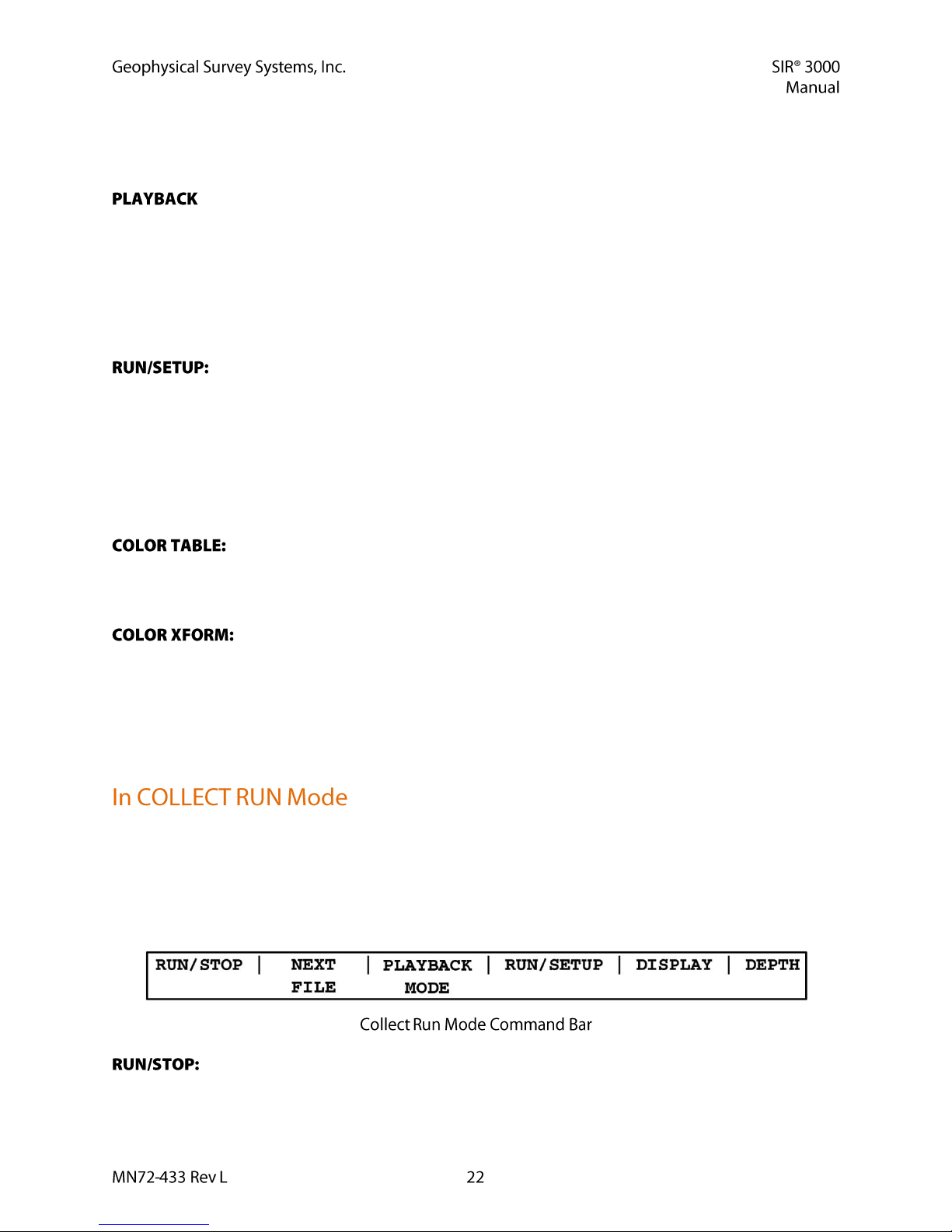
This is what the Command Bar will look like if you are in Collect Run mode. You are in Collect Run
mode if you can see 1 display window. If you see 3 data display windows and the parameter selection
tree), you are in Setup mode.
***You can only collect data in Run mode. ***
In Run mode, the Command Bar will look like this:
Pushing this button in Collect mode will stop data collection and bring up crosshairs.
Pushing this again will close the data file, bring up the Save File window, then start a new data file
collection.
Page 29

Pushing this in Playback mode will toggle the system from Stop to Run and the selected file will scroll
across the screen to the end and bring up crosshairs. Clicking the button after the file has stopped will
cause it to scroll through again.
Clicking this button in Collect Run will stop the current data and bring up the File Save
dialog. After saving the file, the system will immediately begin collecting the next file. This command is
unavailable in Playback Mode.
Clicking this button in Playback Run will bring up the Open File dialog so that you
can select another file to view. Clicking this in Collect Run will close the current collection, ask you to
save the data, and open the Open File window so you can choose a file to view. Clicking this in Playback
Mode will bring up the playback file selection box.
Pushing this in Collect mode will cause the Save File window to come up and close the
current data file. You will then toggle to Setup Mode (3 windows). In Playback mode this key toggles
between Run and Setup.
Pushing this key toggles between a linescan data display and a single scan O-scope style
display. The function is the same in Collect or Playback.
This button allows you to calibrate the system to a target with known depth. This will update the
vertical scale and the dielectric and give you a more accurate depth calculation than simply guessing
dielectric or soil type.
Scan over your area and find a target. Once you do, do not stop data collection, but just move the
system away from that area.
Drill or dig down and measure the depth.
Back at the system, click Run/Stop to bring up crosshairs.
After the crosshairs come up, target them on the first positive peak of that target if it is metal, and the
first negative peak if it is air. Positive peaks stick out to the right (white in a grayscale color table),
and negative peaks stick out to the left (black in a grayscale color table). Push DEPTH and scroll to
the correct depth. Click right to take effect.
If you are on dirt, the dielectric value may only be an approximation.
If you are on a homogenous material, like concrete, this calibration is good for all like material. If you are
on soils, know that the dielectric of the soils can change dramatically with depth and across an area, so
this is only an approximation.
Calibrating the depth in TerraSIRch mode updates the dielectric constant but keeps the fixed time range.
This function in ConcreteScan, StructureScan, UtilityScan, and GeologyScan keeps the entered depth
(under scan) but updates the time range required to scan to that depth given the new dielectric. After
calibrating in one of these four programs (not TerraSIRch) click Run/Stop twice to reinitialize the gains.
Page 30
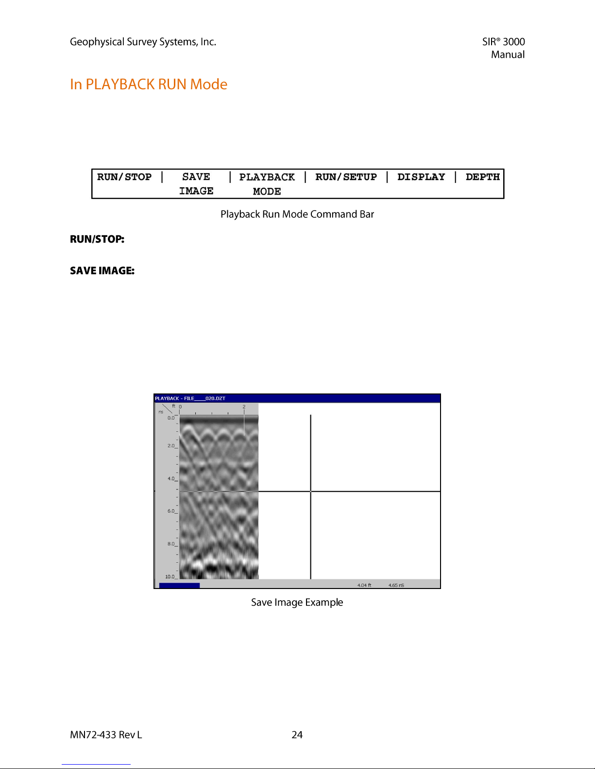
This is what the Command Bar will look like in Playback Run mode. This mode is accessible from the
Playback Setup screen by clicking Run/Setup. After clicking Run/Setup the data file will scroll out to the
end and a set of crosshairs will appear. You can use the arrow keys on the keypad to scroll left and right
to view long data files. The functions here operate very similarly to Collect Setup with two main
differences. These differences are in Run/Stop and Save Image.
This button functions as a screen refresh in Playback Run. Pressing this will cause the data
file to re-scroll from the beginning.
This function will take a screen shot of the data file and save it as a bitmap (.bmp) in your
working directory. Although bitmaps cannot be viewed on the SIR 3000, you can transfer them to a PC
and view, email, or print them later. Bitmaps do not require any special software to view on the PC and
anyone with a PC or Mac will be able to view them. They are automatically transferred when you transfer
a data file and are automatically deleted when you delete that data file. The filename of the bitmap is
similar to the radar data file name. For example, if you are playing back FILE____020.DZT and want to
save an image, then the bitmap will be called FILE____020A.BMP. The “A” tag is there if you want to
take multiple images of the same file. The next bitmap will be called “B”. The Save Image function will
only take a view of the current screen, so if you have a very long data file, then multiple image saves will
be required.
Page 31

In this chapter you will find instructions for configuring your SIR 3000 to collect single 2-D profiles of
data that can be interpreted by themselves or stacked together in software to produce a 3-D image. You
will find instructions for setting up and collecting a 3-D project using the Quick3D Collection mode in
Chapter 4.
The first section of this chapter includes a step-by-step checklist to set up your system. This refers to the
software setup only, not the hardware setup. If you are using a survey cart, please see Appendix C,
otherwise see section 2.1.
These first two parts also assume that you are collecting distance-based data with the survey wheel. If you
are collecting data where the scan spacing is based on time (Time-based), see section 3.3, and if you are
collecting single Point data, please see section 3.4.
If the external memory card is inserted into the system before you turn it on, all data files will be
automatically collected to that memory card. They will not be saved to the internal memory.
Due to constraints on the internal memory, the largest single profile you can collect is 64 MB.
At 512 samples/scan and 12 scans/foot, this translates to 5200 feet, or roughly one mile.
You can collect up to 70 files before you need to power down the system and restart it. If you
collect more than 70 without restarting the system, the SIR 3000 will hang up and you will lose that data
profile that you are collecting and will need to restart the system. Remember to reload any saved setups
and recheck your collection parameters to be sure that they are the same as they were before you powered
down. This may also corrupt your setup file.
After system boot-up, press the TerraSIRch function key. After a few seconds, you will see a split screen
with a wiggle trace on the right, the parameter selection tree on the left, and the main data display window
in the center. If you have an antenna connected, a blue wait bar will scroll twice across the bottom left
corner of the screen (initializing the antenna), and data will appear in the center window.
Examine the parameters in the Collect tree to ensure that the system is properly configured for the
antenna you are using.
Load SETUP
Under the System menu, open SETUP and RECALL a factory setup for the antenna that you are using or
a saved setup that you have worked with previously. A setup will also sometimes contain a preloaded
survey wheel calibration value that makes it easier to use your antenna with a survey cart. These setups
will have the antenna frequency value and then “cart” or “sw.” Setups with cart are for the large three
wheeled survey cart. Those with sw are for the tow-behind survey wheel. For example, if you have a
400 MHz, use a setup which begins with 400.
Page 32

If you are using the 1500 MHz or the 1600 MHz antenna with the blue metal minicart, use
setup 1500BlueCart or 1600BlueCart.
Make sure that MODE is set to DISTANCE. Once you select DISTANCE, the survey wheel calibration
dialogue will come up. You can either enter the factory setting (for smooth terrain) or calibrate it to local
conditions. If DISTANCE already is shown as the selection, you should still check that the calibration is
correct by selecting another choice and then selecting DISTANCE.
In order to manually calibrate the antenna for difficult terrain, you will need to lay out a measured line on
your survey surface. It can be of any length, but the longer the line, the more accurate the calibration.
Enter the calibration distance and position the antenna at the start of the calibration line. The exact part of
the antenna (front, center, rear) that is positioned at the beginning of the line must finish at the end of the
survey line. This is critical for an accurate calibration. Follow the onscreen instructions to calibrate the
wheel. Once you are satisfied with the calibration value, click the right arrow to save this value and exit
the calibration window. Repeat this procedure several times and take the average result.
If you prefer to enter in the value manually, click the mark button to highlight the New Calibration Value
choice and use the up and down arrows to enter in the correct value. Then click the right arrow to save
and exit.
These default values are provided for convenience, but it is always advisable to calibrate
your survey wheel to obtain a more accurate value.
(3 5/6’ wheel):
or single wheel (900 MHz)
2000 ticks/meter
609.6 ticks/foot
(16” wheel ):
400 MHz and 200 MHz tow-behind
417 ticks/meter
127 ticks/foot
Page 33

UtilityScan Cart:
-1785 ticks/meter
-544 ticks/foot
3140 ticks/meter
960 ticks/foot
Blue metal StructureScan Cart with or without bar code reader
4030 ticks/meter
1229 ticks/foot
If you set the horizontal units on the SIR 3000 (under SYSTEM > UNITS > DISTANCE) to
inches or cm, you will need to input the calibration default in ticks/inch(cm). For inches, divide the
ticks/ft by 12 and for cm, divide by 100.
To quickly input a default calibration number, open the calibration dialogue and simply spin the wheel
until the total number of ticks is equal to 10 times the default value.
With the system in Collect Setup mode and data scrolling across the screen, drag the antenna over the
area and find a target that you want to image. Note its position on the screen and at what time/depth it
occurs. Ideally, it should be halfway down the screen so that you can image targets above and below it. If
it is not properly located, change the range under the Scan menu. You may also take one quick profile
over your targets and note where they fall on the data window. If your vertical scale is set to depth, you
can change it to Time under SYSTEM > UNITS > VSCALE. This may help you to estimate the correct
range value.
Page 34

Generally you need a minimum of 10 scans to draw a recognizable hyperbola. The rule of thumb is to
have 10 scans divided by the depth of the shallowest object. So if you want to image something 10 feet
deep, 10 scans / 10 feet = 1 scan/foot. For 5 feet, 10 scans / 5 feet = 2 scans/foot.
For locating structural features in concrete with the 1.5/1.6 GHz antenna, we usually recommend 90/ft.
For utility and tank location, we usually recommend 6-24/ft. While this is more than the minimum rule of
thumb, GSSI has found these densities to work well in the widest variety of situations.
The image below shows hyperbolas from objects of similar size. The hyperbolas vary in size because, due
to the spreading of the radar signal, a deeper target shows reflections in more scans than a shallow one,
The thin, red line superimposed over the scan in the O-Scope window is the gain curve. The centerline of
the scan is zero and to the left of it is negative (decreasing gain) and the right is positive (adding gain).
Ensure that the scan is visible (you can see curves). Gain is applied in dB along an exponential function to
more closely model loss.
If not, select AUTO under the Gain menu. This will cause the system to re-initialize and add/subtract gain
to produce a visible signal. Drag the antenna over the area and look for evidence of clipping. If your data
becomes clipped, leave the antenna over the area where it is occurring and re-initialize by changing
AUTO to MANUAL and then back to AUTO. This will depress the gains so that the data will not clip.
Once you find gain settings which are workable (you can see targets and the signal does not clip), it is
usually best to set the gain to MANUAL. This will allow you to collect multiple profiles that you will be
able to compare without the gains being altered automatically.
Push the function key under RUN/SETUP to begin collecting a profile of data. The system will beep
twice to open the Collect Run window (1 display window) and then beep again when it is ready to receive
data. You can also click the marker button on your antenna handle to open a data collection. At the end of
your profile, push and hold down the Run/Setup key to stop data collection. The profile will be saved and
can be viewed in Playback mode.
Page 35

If you wish to collect another profile with the same settings, you can click NEXT FILE. The SIR 3000
will ask you if you want to save the data. The system is in a paused state, so with that dialog open, move
the system to the beginning of the next profile line and then click Right arrow to save. The SIR 3000 will
save the data and then begin collecting another profile.
Follow these instructions if you want to build a 3D area out of multiple individual survey profiles. You
will save each profile as a different file and create the 3D project in RADAN’s 3D QuickDraw module.
This is an alternative to the Quick3D Data Collection mode discussed in section 3.5.
Follow all the above steps for 2D in order to set your SIR 3000 to local conditions and antenna choice.
After you have set the gains so that you do not clip, set the POSITION and GAIN under the Collect menu
to MANUAL. This will ensure that you do not accidentally auto-gain or auto-position over a different
area while collecting. Gaining over a different area will produce data that is ‘mosaiced.’ Gain differences
will mask features and create edge-effects.
You must lay out your survey grid so that you can cross your targets with at least 3 profiles. Three
profiles will allow you to tell the difference between a point target and a linear target. For example, if you
are looking for graves 2 meters in length, your survey profiles should be spaced no more than 0.5 m apart,
and try to orient your survey grid so that you cross the graves perpendicular to their long axis in order to
have the greatest possibility of hitting them.
In order for your data to be properly positioned in RADAN 5.0 (or higher), you must be able to tell the
software your survey grid origin, line direction, and line orientation. You may begin your survey in any
corner of the grid and survey either in one direction, or zig-zig back and forth.
Collect the data. Collect each survey profile as a separate file. Do not reset the gains or do anything to
cause the system to re-initialize the gains. If you accidentally reset the gains, either reinitialize the system
over the area that you originally set the gains on, or manually enter the gain values you have used
previously. It is best to set the gain to manual before beginning a 3D survey. That way, if you need to
change batteries in the middle of a grid, you will not cause the system to auto-gain. Be sure to keep
accurate notes showing the location of each file in relation to other files and immovable objects. You will
assemble the 3D project in RADAN and 3D QuickDraw after downloading the data to a PC.
Page 36

The scan spacing (horizontal resolution) of Time-based data profiles is a function of the speed that the
system is collecting data and the rate that the antenna is moving over the survey surface. The higher you
set the RATE (in scans/second) and the slower you move the antenna, the denser the data will be.
Time-based data has no real distance tag, so the software has no idea how far you actually traveled. It is
extremely important to move the antenna at a constant speed and to add user marks (by clicking the mark
button) at consistent intervals. Time-based data requires additional processing in RADAN to create a 3-D
image. If 3-D imaging is your goal, you should collect Distance based data with a survey wheel.
After system boot-up, press the TerraSIRch function key. After a few seconds, you will see a split screen
with a wiggle trace on the right, the parameter selection tree on the left, and the main data display window
in the center. If you have an antenna connected, a blue wait bar will scroll twice across the bottom left
corner of the screen (initializing the antenna), and data will appear in the center window.
Examine the parameters in the Collect tree to ensure that the system is properly configured for the
antenna you are using.
Load SETUP
Under the System menu, open SETUP and RECALL a factory setup for the antenna that you are using or
a saved setup that you have worked with previously.
Under the Collect > Radar menu, ensure that MODE is set to TIME.
With the system in Collect Setup mode and data scrolling across the screen, drag the antenna over the
area and find a target that you want to image. Note its position on the screen and at what time/depth it
occurs. Ideally, it should be halfway down the screen so that you can image targets above and below it. If
it is not properly located, change the range under the Scan menu.
This number will be scans per second. Your data density now depends on the rate you move the antenna
over the survey surface. Typically this value is set much lower than the maximum.
The thin, red line superimposed over the scan in the O-Scope window is the gain curve. The centerline of
the scan is zero and to the left of it is negative (removing gain) and the right is positive (adding gain).
Ensure that the scan is visible (you can see curves). If not, select AUTO under the GAIN menu. This will
cause the system to re-initialize and ADD/REDUCE gain to produce a visible signal. Drag the antenna
over the area and look for evidence of clipping. If your data becomes clipped, leave the antenna over the
area where it is occurring and re-initialize by changing AUTO to MANUAL and then back to AUTO.
This will depress the gains so that the data will not clip.
Page 37

Push the function key under RUN/SETUP to begin collecting a profile of data. The system will emit a
beep when it is ready to receive data. At the end of your profile, push and hold down the Run/Setup key
to stop data collection. The profile will be saved and can be viewed in Playback mode.
The third data collection mode on the SIR 3000 is for Point data collection. This mode is most useful for
deep geophysical investigations or data collection over difficult, broken terrain.
In Point mode, we are recording single scans over an area. The scan spacing (horizontal resolution) of
Point-based data profiles is a function of how far apart you set your collection points.
After system boot-up, press the TerraSIRch function key. After a few seconds, you will see a split screen
with a wiggle trace on the right, the parameter selection tree on the left, and the main data display window
in the center. If you have an antenna connected, a blue wait bar will scroll twice across the bottom left
corner of the screen (initializing the antenna), and data will appear in the center window.
Examine the parameters in the Collect tree to ensure that the system is properly configured for the
antenna you are using.
Load SETUP
Under the System menu, open SETUP and RECALL a factory setup for the antenna that you are using or
a saved setup that you have worked with previously.
Under the Collect > Radar menu, ensure that MODE is set to POINT.
With the system in Collect Setup mode and data scrolling across the screen, drag the antenna over the
area and find a target that you want to image. Note its position on the screen and at what time/depth it
occurs. Ideally, it should be halfway down the screen so that you can image targets above and below it. If
it is not properly located, change the range under the Scan menu.
The thin, red line superimposed over the scan in the O-Scope window is the gain curve. The centerline of
the scan is zero and to the left of it is negative (reducing gain) and the right is positive (adding gain).
Ensure that the scan is visible (you can see curves). If not, select AUTO under the Gain menu. This will
cause the system to re-initialize and add/reduce gain to produce a visible signal. Drag the antenna over the
area and look for evidence of clipping. If your data becomes clipped, leave the antenna over the area
where it is occurring and re-initialize by changing AUTO to MANUAL and then back to AUTO. This
will depress the gains so that the data will not clip.
Page 38

Point data is typically collected with some static stacking. The default value here is 64. The system will
take 64 scans at that location and average them together to output a single scan. This is done to minimize
high-frequency, random noise.
Position the antenna at the first data point station and press Run/Setup. You will see the blank, 1-pane
Run screen. Press Run/Stop to collect a point of data. The blue wait bar will scroll at the bottom-left of
the screen while the system is busy recording and stacking your data. When it is finished, the collected
scan number will appear above the Command Bar. Re-position your antenna at the next collection point
and push Run/Stop to collect another point. When finished with the collection, press Run/Setup to return
to the setup screen and save your data.
Page 39

This mode is designed to help you easily collect 3D data on an area of any size and surface. This will
allow you to enter in a grid size and profile spacing and the SIR 3000 will show your current survey
location and guide you through your survey position. During the survey, each individual survey profile is
saved as it is collected, and at the end, the SIR 3000 will create a special folder and file which will
contain positioning information that RADAN needs to display your data. In essence, Quick3D allows you
to skip the 3D file creation step in RADAN.
The next section explains the file structure of a Quick3D file and the sections following explain the field
use and implementation in RADAN of Quick3D files.
The Quick3D data collection mode creates a folder on your SIR 3000 memory card with the name of the
grid followed by the extension .3DS. Inside of that folder are all of the DZT files and a file with the
extension B3D (Build 3D).
DZT files are your actual survey profiles. When you open a radar file in RADAN, you are opening up the
DZT file. In the Windows XP screenshot example below, a 25 foot wide area was surveyed in one
direction only with profiles every 1 foot. We end up with 26 DZT files (1 every foot and the beginning
line) and 1 B3D file. The Grid was named GRID__006.3DS. This grid name was automatically generated
by the SIR 3000.
: The example window is not a SIR 3000 screen image. It is an image from a PC after the data were
downloaded.
The B3D file is an information file which tells the RADAN software where each of your DZT files is
positioned and allows the software to create your 3D file with the proper positioning information. To
open the grid in RADAN, you need to open the B3D file. In RADAN go to FILE > OPEN and change the
Save as Type to 3D Project File. It will have defaulted to DZT file. You may have to click Open once in
order for Windows to display the B3D file.
When you transfer your data from the SIR 3000 to a PC running RADAN, you must transfer the whole
Grid folder. Furthermore, do not remove the files from the Grid folder. Keep all files pertaining to that
grid in the Grid folder.
Page 40

So, to sum up: each grid you collect is a separate folder. Inside that folder are all of your radar data lines
(DZT files). Also inside that folder is the B3D file which you will open in RADAN. Once RADAN reads
that B3D file, it will know which of your data lines to put where. You must keep that B3D file and all
of you data files together in the same grid folder.
Collecting data for 3D imaging is easiest when you have a guide grid laid out to follow. You should lay
out a grid with chalk, paint, ropes, or some other method. Your grid can be any size, but your data quality
will be much better if you make sure that your grid corners are square. Your grid itself does not have to be
a square, it can be a rectangle, or can be irregularly shaped, but if you follow the tips below, you will save
yourself a lot of trouble.
If you are scanning in one direction only with a normal profile order (one direction only), you need
the grid edge that you start your profiles from (the baseline) to be straight. We understand ‘one
direction only’ to mean scanning along only the X or the Y axis, but not both. A ‘normal’ profile
order is one where you are collecting data along your profile in one direction. In other words, you
start at the baseline, collect your data until the end of the line, pick up your system and move it back
to the baseline to collect the next profile in the same direction. This is different from zig-zag where
you are simply turning around and collecting the next data file in the opposite direction from the
previous. If you are collection with a zig-zag order, both the start and finish baselines should be
straight.
Your grid can be irregular, but as long as the line that your profiles start from is straight, the
RADAN software will have no problem lining things up.
Make sure that your grid corners are right angles and that your grid lines are actually perpendicular
to your baseline. The graphic below illustrates how to put together a square, 10×10 grid.
Locate the origin point (0,0) and pull a tape measure 10 to
find the point 10,0 (blue line: a). This is your baseline.
Pull one tape measure 10 from 0,0 (line b) to 0,10. Pull the
other one from 10,0 to 0,10 (line c).
Move both tapes together so that 10 on line b connects to
14.14 on line c. The point that they connect is the grid
corner. You will know that the corner at 0,0 is square
because this method produces a right triangle.
Repeat for the corner 10,10.
You can use this method for grids of any size. You can also use this for rectangular grids.
Make sure to assign X to one axis and Y to the other.
Photograph or make a sketch map of the grid.
Page 41

Pictured at the right is the full Collect Menu tree from the Quick3D
mode. The blue boxes enclose the menu choices which are new to
the Quick3D. The following sections explain what they are and
present a step by step guide to set up the software.
This menu controls the grid size, profile line spacing,
and survey direction.
Normal/Zig-Zag. This controls the survey line direction.
Normal profiles are all surveyed in one direction. At the end of
each line, you must move the antenna back to the starting baseline
before moving to the next line and collect along that same direction.
A zig-zag order allows you to collect data in both directions.
These two items tell the system the coordinate of your
origin point. Typically these will both be 0. If you are working on a
pre-existing site grid and you want your survey grid origin to have
that coordinate, you can put it in here.
The SIR 3000 uses this coordinate to figure out the size
of your grid. In the menu tree, the numbers for both the X and Y are
20. This means that the X axis and the Y axis both end at 20, and
since the origin is at 0,0 the grid is 20×20.
These numbers are coordinates, not line length. So if you
have a 20×20 grid and X/Y START is 10×10, then X/Y END is
30×30.
This is the spacing between your survey lines. X
lines are parallel to the X axis and Y lines are parallel to the Y axis.
The X spacing can be different from the Y spacing, but the spacing
must be regular. For example, you cannot start your grid at one interval and change halfway through to
another. If you need to change the line spacing, you must start a new grid with the new parameters. If you
only want to collect on the X or the Y, set the line spacing of the direction you are not collecting to 0.
If you intend to collect data in both X and Y and to process that data, you must collect the grid
twice: once in X and once in Y, and then combine them in RADAN.
Page 42

This function allows you to test the dielectric of the material you are scanning through by
Hyperbolas have not
collapsed into points.
Still are shaped like
hyperbolas.
Hyperbola tails have
turned upward into
‘smiles.’
Hyperbolas have
collapsed into narrow
targets.
collecting a section of data and then performing a migration on that data. This is important because if
your dielectric is correct, then you know what depth you are scanning to. Highlight this choice and click
Enter to bring up a pop-up menu. You will notice that data has stopped scrolling across the screen. With
that pop-up menu on the screen, collect a profile of at least 10 feet in length. This profile must go over
known targets and must cut across those targets at a right angle. You will now use the Up and Down
arrows to adjust the dielectric value so that those hyperbolas collapse to points. After selecting a dielectric
value, press Enter to see that take effect. Once you have established the correct dielectric value, click the
Right arrow. This will also cause the system to re-initialize.
Dielectrics in soils are rarely constant. This method is best suited to find the dielectric in engineered
or homogenous materials. Do not use this method to establish a depth approximation in soils.
After system boot-up, press the Quick3D function key. After a few seconds, you will see a split screen
with a wiggle trace on the right, the parameter selection tree on the left, and the main data display window
in the center. If you have an antenna connected, a blue wait bar will scroll twice across the bottom left
corner of the screen (initializing the antenna), and data will appear in the center window.
Under SYSTEM > SETUP > RECALL, find the appropriate Setup. Highlight the one that you want and
click the Right arrow to load it. Note that the SIR 3000 will reinitialize. Wait for the data to start scrolling
across the screen before continuing. Please see Appendix E for a list of saved Setups. If you do not wish
to use one of the saved Setups, you should still recall the Setup that closely matches your antenna’s
frequency. You should then modify that Setup accordingly.
Page 43

This is a critical step in 3D file collection because proper positioning of your data is so important.
Make sure that MODE is set to DISTANCE. Once you select DISTANCE, the survey wheel calibration
dialogue will come up. You can either enter the factory setting (for smooth terrain) or calibrate it to local
conditions. If DISTANCE already is shown as the selection, you should still check that the calibration is
correct by selecting another choice and then selecting DISTANCE.
In order to manually calibrate the antenna for difficult terrain, you will need to lay out a measured line on
your survey surface. It can be of any length, but the longer the line, the more accurate the calibration.
Enter the calibration distance and position the antenna at the start of the calibration line. The exact part of
the antenna (front, center, rear) that is positioned at the beginning of the line must finish at the end of the
survey line. This is critical for an accurate calibration. Follow the onscreen instructions to calibrate the
wheel. Once you are satisfied with the calibration value, click the right arrow to save this value and exit
the calibration window. Repeat this procedure several times and take the average result.
Under the COLLECT > 3D-GRID menu, set your grid limits and line spacing. Normally the X-START
and the Y-START should both be set to 0. If your grid is not starting at 0,0 you should put in the
coordinates of the origin point here. The only time that you would not want your grid to start at 0 is if it is
just a small part of a larger site grid. If you are going to combine grids later in Super3D, you can just
leave this number at 0,0 and add real coordinates later. Just remember that your X-END and Y-END are
coordinates, not line lengths. If you intend to process the data, you should only collect a 3D file along
either the X or the Y, not both. If you want 3D with both directions, you must collect the area twice. For
the X, set up the file with a 0 in the Y line spacing, and vice versa if you want to collect for the Y. Collect
and save the file, then collect and save a separate file for the other direction. You will thus end up with
two 3D files.
Push the function key under RUN/SETUP to begin data collection. The system will beep twice to open
the Collection Run window (2 display windows). You will see the Linescan window at the right (it will be
blank at first), the Position window at the left, and the Prompt Area at the top. Position your antenna so
that its center is in the middle of your start line and push the Mark button.
The ‘MARK TO START’ message will turn into a ‘COLLECT DATA’ message. Move the antenna along
your survey line. You will see data scrolling across the screen. Once the SIR 3000 has collected enough
data (based on your setup parameters), it will stop recoding automatically. Reposition your antenna at the
beginning of the next line and continue by following the instructions shown in the Prompt Area.
Page 44

After you have clicked RUN/SETUP from the
setup screen, you will see the Run screen
(2 windows at right). You will need to click the
Mark button on the SIR 3000 to start data
collection. Each successive line can be started
with the remote marker switch on your antenna.
The Prompt Area tells you positioning
information and also what to do during
collection. The image at the right tells you at that
you are on your second line, you are scanning
parallel to the X direction, and that you should be
on the 1 foot mark along your Y baseline.
Once you have clicked the Mark button, you will see COLLECT DATA in the prompt area. Wait for the
green light to come on next to the RUN/STOP button. Collect the profile line. Once you have gone the
distance that you specified in the Setup, the SIR 3000 will stop collecting data automatically. It will save
the file and automatically increment to the next line.
If you need to skip or redo a profile, use the arrow keys to highlight that file and then press Mark. The
new data file will then be stored with the proper positioning info and any old data will be overwritten.
You can go directly into Playback by clicking the Playback
Mode button.
Your data will be automatically saved and it will generate
a top-down view.
Depending on the size of your collected area, this could
take anywhere from seconds to minutes. Be patient.
(previous section, 2 windows)
Page 45
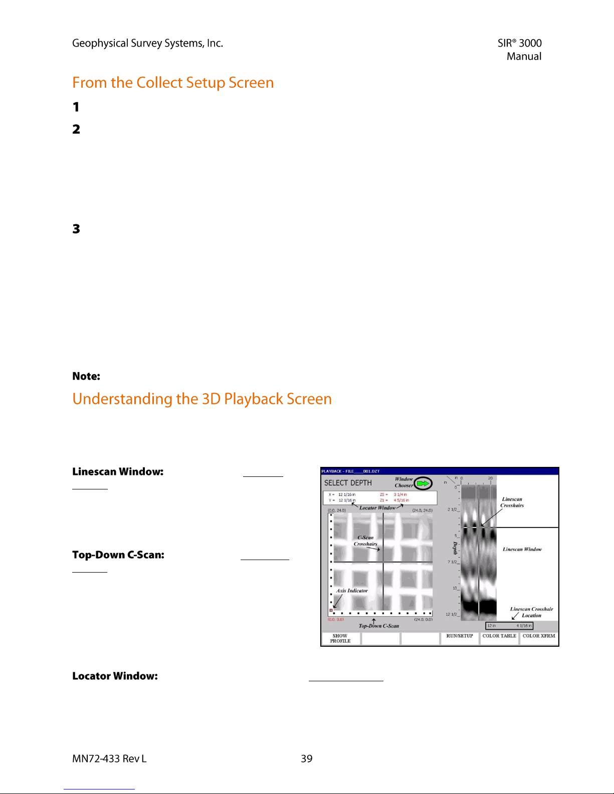
(3 windows with the parameter selection tree at the left)
Click the Playback Mode button. You will see a pop-up window with all of the stored data.
Choose the grid file you want to play back and click the Right arrow. The data will scroll across the
screen.
You can change the Display Gain setting (OUTPUT > DISPLAY > GAIN) or any of the process
settings, including toggling the Migration on and off and selecting the proper material dielectric
for that migration.
A table of dielectrics of common materials can be found in Appendix D.
When you have made the necessary changes, click Run/Setup to go to Playback Run. The SIR 3000
will generate the top-down view of your area.
Depending on the size of your collected area, this could take anywhere from seconds to minutes.
Be patient.
The SIR 3000 will also process the data by applying a background removal filter to take out constant
horizontal banding (including the direct wave). If you have the Migration process turned on under the
PLAYBACK > PROCESS menu, then the computer migrates with the dielectric that you have specified
under PLAYBACK > SCAN. Just like under the Test_Diel function in Collect Setup, if you have too low
a dielectric specified, the hyperbolas will turn into ‘smiles.’ If you have too high a number, they will
remain hyperbolas.
The SIR 3000 is only performing a constant velocity migration.
Once you get to this display you can toggle to different color tables or transforms by using the Command
Bar buttons, or go back to the Setup (3 windows) screen by clicking Run/Setup.
The C-scan (top-down) display window is split into 3 important areas.
At the right is the Linescan
window which shows a 2D vertical profile. Depth is
shown on the vertical axis and distance along the
survey profile is shown on the horizontal. Underneath
this display are two coordinates. The first is distance,
and the second is depth.
At the left is the Top-Down
C-Scan map. This map shows the location of targets
as if you were standing above your survey area and
looking straight down. At the lower left corner is 0,0.
The X axis is horizontal and the Y is vertical. The
black dots along two of the sides are the locations of
profiles. You will also see a red box (Axis Indicator)
covering one of the dots. That is the currently
selected profile and the one that will be displayed in the linescan window if you press Show Profile.
Above the C-Scan window is the Locator Window. This window gives positioning
information for the C-Scan crosshairs and also shows the highest (Z0) and lowest (Z1) points of the depth
slice shown in the C-Scan.
Page 46

The C-Scan display has three main functions: Select Depth, Select Profile, and Select X/Y Position. You
toggle between each one by clicking Enter. When you click Enter, the window chooser arrow changes.
This arrow shows you which window (Linescan or C-Scan) to browse with the arrow keys.
For example, if you click Enter until the Select X/Y Position wording appears, you will notice
that the window chooser arrow points down to the C-Scan window. Now if you click the arrow
keys, you will notice that the C-Scan crosshairs move and you will get location information in the
Locator Window.
You may also see the first number change in the Linescan Crosshair locator, but the locator
window information is more accurate. Each of the modes are explained below.
This mode allows you to find the horizontal location of targets or clear areas to
drill. The window chooser arrow will point down to the C-Scan window, telling you that you should only
work with this window to make decisions.
You can move the C-Scan crosshairs around with the arrow keys to get locations on anything you
see in the data.
You will also notice that the vertical crosshair on the Linescan Window is also moving and that it
is giving a location below that window (right above the Color Table button). That location is not
as accurate as the one on the C-Scan window. You should always read X/Y coordinates from the
C-Scan Locator Window.
You MUST pay close attention to the Z0 and Z1 numbers on the C-Scan Locator Window. The
C-Scan is only showing targets within that depth range. For example, in the screenshot on the previous
page, that map is of targets between 3 ¼ and 4 5/16 only. Anything above or below that depth is not being
displayed.
Page 47

This mode allows you to find out how deep
something is and to change the display depth of the C-Scan window.
You will notice that the Window Chooser arrow is pointed to the
Linescan Window on the right.
If your scan is 12” (or up to 50 cm) deep, then it will be
divided into 12 equal slices.
If it is deeper than this, then it will be divided into 15 slices.
You will use the Up/Down arrow to move the horizontal
crosshair on the Linescan Window up and down. That will
give you depth information which will be displayed below
the Linescan Window (above the Color Xform button).
Page 48

Remember that the top of a piece of metal is the middle of the first bright white part of the target.
In the example on the right, the black dot is at the middle of the white target which is the location
of the top edge of the metal target. In order for this to be true, make sure that you are in the
grayscale color table and that the positive amplitudes are being displayed as white. To get the
depth of that you should set the horizontal linescan crosshair at that location.
If you scroll to the top or the bottom of the image, you will get a C-Scan display of the full depth
range. The image is displaying strongest targets in the full range. If you look at the C-Scan
Locator Window, you will see that Z0 is set to 0 and that Z1 shows the maximum depth.
Otherwise as you scroll up and down the profile, these numbers will change once the horizontal
crosshair on the Linescan Window crosses a distance threshold. The C-Scan will then change to
show the new slice data and the Z0 and Z1 will update to give you the new depth range.
The accuracy of the depth reading is 100% dependent on your accurate guess of the dielectric.
Remember that dielectrics in soils often change with depth, and since the SIR 3000 is performing a
constant velocity migration, then it will not take those changes into account.
This mode lets you display individual profiles in the Linescan Window at the right. You
would do this to show a target that you can then find the depth of by using the Select Depth mode. You
will notice that the window chooser arrow is now pointing down to the C-Scan window.
You can select the X profiles by clicking Up/Down and the Y profiles by clicking Left/Right. The
profile line number will be displayed in the C-Scan Locator Window.
Once you have selected your profile, click the Show Profile button on the Command Bar to
display it in the Linescan Window. Each profile begins at the red box and ends at the tip of the
arrow. In the Linescan Window, the profiles read from left to right with the beginning (red box
location) being at the left.
Page 49

Page 50

This section describes how to transfer data from the SIR 3000 to a PC for processing and interpretation,
and also how to clear unwanted data from the system’s memory. These functions are all accomplished
under the Output menu.
If the external memory card was inserted into the system before you turned it on, all data files were
automatically collected to that memory card. They were not saved to the internal memory.
If this is your first time transferring data via the USB connection, please see Appendix G: Installing
Microsoft ActiveSync on Your PC.
Turn on PC and SIR 3000. (If SIR 3000 has been running, stop all collection and playback functions
prior to continuing) Connect Master (rectangular) end of USB cable to computer. Connect Slave
(square) end of USB cable to SIR 3000.
Enter the TerraSIRch mode and click Run/Stop to pause the system.
Under the OUTPUT > TRANSFER submenu, click on PC.
Wait for ActiveSync light to turn green and then right click on green ActiveSync icon located in
system tray. Next click Explore; you will see the mobile device explorer. You are now accessing the
SIR 3000’s memory.
Navigate to My Computer > Storage Card and go to the folder containing your projects. You will now
be able to copy from one location on the storage card to the external storage card or to a folder on the
PC by ‘drag and drop.’ When transfer is complete (wait a couple of seconds after completion)
disconnect USB cable from SIR 3000.
Turn on PC and SIR 3000. If the SIR 3000 has been running, stop all collection and playback
functions prior to continuing. Make sure that your Flash card is inserted AFTER powering up the
system.
Enter the TerraSIRch mode and click Run/Stop to pause the system.
Under the OUTPUT > TRANSFER submenu, click on FLASH.
A window will appear showing all files on the internal memory. Highlight the files and click Enter
once on each file to add a ‘check’ next to them. Once all files are ‘checked,’ click the Right arrow to
begin the transfer. This process will not delete the data from the internal memory.
Remove Compact Flash card from the SIR 3000 and insert it into a USB CF card reader or similar
and attach the card reader to your computer. You can now access the data as if you had another disk
drive on your computer.
Page 51

If you get an Error #3, this indicates that the SIR 3000 has not recognized the card. Pop the card out,
wait 5 seconds and reinsert.
This choice is available to allow you to use a USB ‘memory stick’ to transfer your data.
Any keychain drive that requires installation, drivers, or restart of a computer in order to have it
recognized will not work with the SIR 3000. GSSI has tested the Attaché USB 2.0 Flash drive by PNY
Technologies and has found it to work.
Turn on PC and SIR 3000. If the SIR 3000 has been running, stop all collection and playback
functions prior to continuing. Make sure that your memory stick is inserted AFTER powering up the
system.
Enter the TerraSIRch mode and click Run/Stop to pause the system.
Under the OUTPUT > TRANSFER submenu, click on HD.
A window will appear showing all files on the internal memory. Highlight the files and click Enter
once on each file to add a ‘check’ next to them. Once all files are ‘checked,’ click the Right arrow to
begin the transfer. This process will not delete the data from the internal memory.
Remove the USB Keychain/Pen Drive from the SIR 3000 and insert it into a USB port on your
computer. You can now access the data as if you had another disk drive on your computer.
While it is always advisable to keep the data on your system until you have downloaded it (if desired) and
checked the integrity of the data, eventually the memory may fill up or you may simply want to do some
‘housecleaning.’ GSSI suggests that you download all of the data from a particular jobsite and
completely delete the data before starting a new job. This will help to avoid confusion over which files
belong to specific projects.
Highlight Delete under the TRANSFER submenu, and push Enter. You will see a window with a list
of files.
Using the Up and Down arrow keys, highlight the file to be deleted and push Enter to place a ‘check’
in the empty box to the left of the file name.
Repeat until there are ‘checks’ next to all of the files you want to delete. Click the Right arrow key to
accept and delete those files.
When you attempt to collect a new file, the system will find the lowest number it can to assign to
the new file. For example: if you have 25 files, and you delete File_001, the next file will not be File_026,
it will be File_001. In other words, it will fill in any gaps in the memory before adding new files.
Page 52

The section briefly describes four out of the six operation modes for the SIR 3000. These modes are more
limited in their customization because they are meant for specific applications or to collect data for onscreen target location as opposed to post-processing. As noted earlier, TerraSIRch mode allows you full
reign over all collection parameters. The 3Dscan mode is similar to TerraSIRch in that it is fully
customizable, but with the added feature of defining an easy 3D data collection project. Please note that
some of these modes may require additional equipment purchase in order to get full functionality.
Expanded instructions for each of these modes are available in the form of separate QuickStart manuals.
Contact your GSSI sales consultant for more details. The four additional modes are:
ConcreteScan
StructureScan
UtilityScan
GeologyScan
ConcreteScan is meant for a ‘quick and dirty’ scan of concrete. You would use this mode to locate
shallow structural features in concrete and mark their location directly on the survey surface prior to any
cutting, coring, or drilling. It works with the 2.6 GHz, 1.6 GHz, 1.5 GHz, 1.0 GHz and 900 MHz
antennas.
First choose English or Metric units and then click on the ConcreteScan button. You will then see the data
display screen and, if an antenna is connected, it will initialize and data will start to scroll across.
ConcreteScan includes the backup cursor function. This allows you to back the antenna over the line you
just surveyed and get an on-screen cursor that will help you relate the location of targets in the data back
to the slab. The backup line in the data is the location of the midpoint of the antenna.
You will choose your antenna (2.6 GHz, 2.0 GHz Palm 1.6 GHz, 1.5 GHz, 1.0 GHz or 900 MHz) under
the RADAR submenu, and also select DISTANCE or TIME based collection under MODE. Remember to
check the survey wheel calibration if you are using DISTANCE.
Under the Scan submenu, choose your maximum penetration depth from a number of presets:
6, 12, 18, 36 inches, or 15, 30, 50, 100 cm.
Select your SCN/UNIT from 5/7.5/10 per inch or 2/4/5 per cm.
Also set your concrete type from a number of presets ranging from Dry to Wet. This sets the dielectric
constant and gives you a rough depth calculation.
Page 53

T_RATE: 100
Samples/Scan: 512 deep, 256 shallow (12” and less)
Format/Bits: 16
RATE: 100 (deep) 200 Shallow (12” and less)
Gain: 5 point Auto
Filters (All)
Offset position
Surface position
This mode is for collecting very high-resolution 3D data over a concrete slab or wall with the 2.6 GHz,
1.6 GHz, 1.5 GHz or 1.0 GHz antenna and GSSI’s patented scan pad. This will produce a 3D cube of data
that can be viewed in planview at differing depths so as to note clear locations for coring and cutting. You
must use the scan pad for this mode and collect data in a prescribed fashion. Consult the StructureScan
QuickStart guide for more details.
Under the Scan submenu, choose your maximum penetration depth from a number of presets: 6, 12, or 18
inches, or 20, 30, 50 cm.
Also set your concrete type from a number of presets ranging from Dry to Wet. This sets the dielectric
constant and gives you a rough depth calculation.
T_RATE: 100
Samples/Scan: 512 deep, 256 shallow (12” and less)
Mode: Distance
Format/Bits: 16
RATE: 100 (deep), 200 shallow (12” and less)
Scn/Unit: 5/inch, 2/cm
Gain: 1 point Auto
Filters (All)
Offset position
Surface position
Page 54

UtilityScan is meant for a quick examination of an area in order to locate utilities in soils under concrete
slabs or asphalt. UtilityScan can be used with the 270 MHz, 400 MHz, and 900 MHz antennas. Both the
400 MHz and the 270 MHz can be used with the survey cart. UtilityScan will allow you to create 2D
profiles so that you can mark the location of utilities on pavement prior to trenching or excavation.
Upon clicking the UtilityScan button, you will be asked to click Right for English or Left for Metric units.
You will then see the data display screen and, if an antenna is connected, it will initialize and data will
start to scroll across.
UtilityScan includes the backup cursor function. This allows you to back the antenna over the line you
just surveyed and get an on-screen cursor that will help you relate the location of targets in the data back
to the slab. The backup line in the data is the location of the midpoint of the antenna.
Choose your antenna by selecting the proper center frequency from the list under the Radar submenu.
Select DISTANCE based or TIME based data collection under MODE. Remember to check the survey
wheel calibration. Choose 512 (recommended) or 256 samples/scan under the SAMPLES submenu, and
then choose 16 (default) or 8 bit data collection under FORMAT.
Next select your maximum depth of penetration from the list of 5 presets (3, 5, 10, 15, 20 ft) (1, 3, 5, 7
meters). Select the appropriate soil type from the list of 4 presents (Soil Type 1-4). This will set your
dielectric and affect your maximum depth of penetration.
Then select your scans per unit from the list of presets. GSSI recommends a scan density of either 12 or
18 per foot, or 25 per meter.
Type 1: Dielectric 4, dry sand or dry grade
Type 2: Dielectric 8, damp sand or grade, dry silt
Type 3: Dielectric 16, agricultural fields, sandy silt, wet sand
Type 4: Dielectric 32, wet conditions, clay
T_RATE: 100
RATE: 100
Gain: 3 point Auto
Filters (All)
Offset position
Surface position
Page 55

This mode is optimized for 2D profiling of shallow geological features such as high bedrock, sediment
bedding, water tables, etc. It is also useful for archaeological profiling. GeologyScan works with the 400
MHz, 270 MHz, 200 MHz, and 100 MHz antennas, though only the 400 and 270 MHz are small enough
to be mobilized on the survey cart. Other antennas will need to be dragged over the ground surface.
Upon clicking the GeologyScan button, you will be asked to click Right for English or Left for Metric
units. You will then see the data display screen and, if an antenna is connected, it will initialize and data
will start to scroll across.
There is no QuickStart Guide available for GeologyScan.
Choose your antenna by selecting the proper center frequency from the list under the RADAR submenu.
Select DISTANCE based or TIME based data collection under MODE. Remember to check the survey
wheel calibration. Choose 1024 (recommended), 512, or 256 samples/scan under the Samples submenu,
and then choose 16 (default) or 8 bit data collection under FORMAT.
Select the appropriate soil type from the list of 4 presents. This will set your dielectric and affect your
maximum depth of penetration.
Then select your scans per unit from the list of presets. The presets are 6, 12, 18 per foot for English, or
10, 25, 50 per meter for Metric units.
T_RATE: 100
RATE: 80
Range: Max for antenna
Gain: 5point Auto
Filters (All)
Offset position
Surface position
Page 56

Your SIR 3000 is capable of attaching GPS coordinates to individual data profiles. This will allow you to
place the beginning and the end of your survey lines into a larger, real-world coordinate system provided
that you: 1) Survey in straight lines and 2) Have a GPS with sufficient accuracy for your application.
GSSI will publish specific integration information as a series of Technical Notes available on the GSSI
Technical Support website at .
Attaching a GPS with its own data logger, such as the G30L available from GSSI, will allow you to
collect GPS data points with a much finer resolution. RADAN 6 will then be able to wrap data files and
show coordinates with a GPR X, Y, and Z.
The GPS you do choose must have the following:
1. Provide data output through a serial (RS232) port.
2. Output data at a baud rate of 4800.
3. Output the NMEA GGA data string.
GSSI only supports the G30L receiver or integration with the Acumen serial data bridge logger
available from GSSI.
Try your GPS to determine if you are getting a good position and an adequate number of satellites.
Setup and power up your SIR 3000 as normal.
Under COLLECT > RADAR, highlight the GPS menu choice and click Enter. Toggle to G30L for
the GSSI provided receiver or to CUSTOM for any other receiver and click the Right arrow.
The Enable GPS dialogue box will pop up. Follow the instructions in the window to connect your
GPS. You should ensure that your receiver is tracking at least 4 satellites. If you are using the G30L,
4 is the minimum number of satellites you can use.
When you start a data profile, the SIR 3000 will capture a GPS coordinate and place it in the file
header. It will do the same when you stop the data file and save it. These coordinates will be visible
when you view the file header in RADAN 5.0 or higher.
The .TMF file. You will notice that the SIR 3000 has created 2 files: the data profile (.DZT) and
another file with the same name but a different extension (.TMF). This file will be used for some
added GPS functionality which is not yet available.
East vs. West. The SIR 3000 is set to capture Latitude and Longitude coordinates rather than UTM.
It does not however tag a North/South or East/West to those numbers. If you are west of the Prime
Meridian, the Longitude will be negative and if you are south of the Equator, the Latitude will be
negative.
Page 57

This is a brief description of GPS and how to use it with our SIR 3000. GPS information gets attached to
Ionospheric
Refraction
Tropospheric
Refraction
MultiPath
Reflection
GPS
Satellite
Ionospheric
Refraction
Tropospheric
Refraction
MultiPath
Reflection
GPS
Satellite
our data two different ways. First, the start and end positions are stored in the header of each *.DZT file.
Second, the timing of each marked scan is stored in a separate *.TMF file, which RADAN 6.0
incorporates into its database.
This paper gives a quick GPS overview and then describes what you need to know in order to effectively
use the SIR 3000 with a GPS.
GPS is a satellite navigation system (provided free by the USDoD) designed to provide
instantaneous position, velocity and time information almost anywhere on the globe at
any time, and in any weather. It typically provides positioning accuracies ranging from 3
meters (costing $150) to 1cm ($15,000). Since it needs to see much of the sky, it works
poorly indoors, in woods and in “concrete canyons” like Manhattan.
You probably don’t! In fact for many Ground Penetration Radar applications you can just use a survey
wheel to measure your distance and take simple notes about your start and stop locations. And since
digging or drilling often requires more precision than 3meters, knowing “sort of” where you are is not
helpful.
However, as surveys become larger and as technologies improve, GPS can be very helpful in telling you
where you are on a map, or what road you turned onto, or what section of the avalanche you have already
covered, or even where you were in the middle of a lake. And of course if you actually need expensive
survey-grade GPS accuracy, we want to give you the hooks you need to place our RADAR data correctly.
Increasingly GPS is claiming a legitimate place in the ever increasing size and variety of GPR
applications.
GPS works by triangulating the distance from satellites in space. Like our
RADARs, these satellites just transmit time very accurately and estimate the
distance using the speed of light. Getting the travel-time from just three
satellites is enough to know where you are on the earth. Getting the traveltime from 12 satellites greatly decreases the uncertainty of your position.
Typically around buildings and trees you might “see” six satellites, plenty to
know where you are to within 3 meters. The degree of precision depends on
many things, like how well distributed the satellites are in the sky, or the
travel path the signal took to get to your receiver.
GPR and GPS share a lot in common. The travel times and paths are directly affected by the medium. For
GPS, this means the signal from the satellites to your receiver can get slowed down and bent by changes
in the Ionosphere, the Troposphere and even nearby objects. These sources of error can be reduced using
expensive tricks like dual frequency, Klobuchar modeling and Real-Time Kinematic (RTK) solutions.
Page 58

The least expensive way to correct for these errors is through Differential GPS (DGPS), where data from
a second stationary “Base” GPS is subtracted from a Roving GPS. Compared to the distance from the
satellite, distance between Base and Rover is insignificant, which means the travel paths through the
ionosphere and troposphere are basically identical. So the difference between the two positions subtracts
out atmospheric effects, leaving just the Rover position.
The Wide Area Augmentation System (WAAS) is a form of differential GPS that uses geostationary
satellites to transmit an error correction estimate back down to your receiver. The measured positions of
ground reference stations, strategically positioned across the country, are sent up to the WAAS satellites.
Your receiver reads the reference station closest to you.
“WAAS testing in September 2002 confirmed accuracy performance of 1 – 2 meters horizontal and 2 –3
meters vertical throughout the majority of the continental U.S. and portions of Alaska.”
( ) This is with a clear view of the sky. Typically WAAS
can improve your error from less than 5 meters 95% of the time to less than 3 meters. WAAS is now
available even in the less expensive GPS units and is recommended.
The National Marine Electronics Association ( , pronounced “NEE’ma”) has generated a standard
set of messages for communicating GPS information. We use the NMEA 0183 version 2.1 protocol.
We have chosen to go with a GPS Datalogger, mostly because it is so simple. No buttons, nothing to
control and everything is handled automatically inside the SIR 3000. Yet it produces results as good as
the other consumer-grade, WAAS enabled units.
However if you already have a GPS, we have tested the Garmin eTrex, GPS Map76S, Magellan SporTrak
Pro, Teletype PocketPC GPS, and a few others. These should all work fine, but not as seamlessly.
Our requirements are rather flexible. Any unit that sends the NMEA GGA command should work. Since
each company sells its own interface, we have chosen to work with the popular shareware, OziExplorer
( ), as our interface. Oziexplorer can talk to Garmin, Magellan, Eagle, Lowrance,
Brunton/Silva and MLR units. It will even interface with other NMEA compatible units that output
waypoints in the NMEA sentences:
$GPRMC or
$GPGGA and $GPVTG or
$GPGLL and $GPVTG
If your GPS outputs a GGA command every second in a standard serial fashion (4800 baud, 8 bit, no
parity,1 stop bit), and if you can get your tracklog into OziExplorer, then we can talk to your GPS with
RADAN 6.0.
Page 59

The G30L was an optional accessory to our SIR 3000. It is no longer available new and this section is
presented for those who had previously purchased the G30L. It is a GPS datalogger with no external
controls. It will store up to 15 hours of GPS data that can be downloaded at any time. The only caveat is
that once it fills its memory, it stops. For this reason, we stop and clear its internal memory at the end of
each survey. To simplify the interface we also needed to make changes in RADAN, which will next
appear in version 6.0. Here’s all you need to do.
Turn on your SIR 3000.
Plug your GPS unit in the serial port and the USB port (for power)
Enable GPS in the RADAR Menu (always off on Startup).
GPS Start/Stop positions and times go in the header of your DZT data file. (see Addendum A). These
positions are all you’ll need for most surveys.
The GPS positions between Start and Stop get matched up with the Mark positions in RADAN 6.0 and
are stored in the new database (Microsoft Access compatible).
First Collect the GPS/GPR Data.
Turn on your SIR 3000.
Plug your GPS unit in the serial port.
Enable GPS in the RADAR Menu (always off on Startup).
Set your GPS to output NMEA (the standard 0183 version 2.1) at 4800 baud.
Set your GPS to start logging track data. On the Garmin units this means going to the “Track” menu,
turning it on and setting the track interval (i.e. every 2 seconds or every 10meters.)
Start Data Acquisition:
Stop Data Acquisition and Close the file.
GPS Start and Stop positions and times go in the header. In our header, rh_version is set to 2. (see
Addendum A).
So far this is not complicated at all. And since most surveys will require nothing more than these two
begin/end positions, any standard GPS outputting GGA will do this job nicely.
Next Time-Synchronize GPS/GPR files.
But if the survey is along a curve, you will need to work out the GPS position of each scan.
This can be done in Microsoft Visual Basic or with Simulink MatLab to get the two data files together.
Page 60

Our Binary file extension is *.TMF. The tracklog output of your GPS software will have a unique
extension. (that’s why we prefer the Oziexplorer *.plt file so that all the various GPS’s can output data in
one format).
For based data acquisition.
Match GPS Start/Stop position/time with records in the GPS log.
The scan rate is used to time tag individual scans.
For based data acquisition or data with user marks.
Match GPS Start/Stop position/time and file filename.TMF (see Addendum B) to synchronize
marked scans with the time/position records from the GPS log. Interpolate time/distance data between
the marked scans as necessary.
Please see the protocols listed below in the following Addenda for help on how to extract the necessary
information.
Page 61

This information is being provided for informational use only. It is not supported by GSSI
technical support and is only provided for those users who are already comfortable working in a C
programming environment.
struct tagRFDate // File header date/time structure
{
unsigned sec2 : 5; // second/2 (0-29)
unsigned min : 6; // minute (0-59)
unsigned hour : 5; // hour (0-23)
unsigned day : 5; // day (1-31)
unsigned month: 4; // month (1=Jan, 2=Feb, etc.)
unsigned year : 7; // year-1980 (0-127 = 1980-2107)
};
struct tagRFCoords // Start/End position
{
float rh_fstart;
float rh_fend;
};
struct RGPS // GPS record/system time SYNC
{
char RecordType[4]; // “GGA”
DWORD TickCount; // CPU tick count
double PositionGPS[4]; // Latitude (positive if 'N'), Longitude (positive if ‘E’),
// Altitude, FIXUTC
};
// constants
const int MINHEADSIZE = 1024;
const int PARAREASIZE = 128;
const int GPSAREASIZE = 2 * sizeof(RGPS);
const int INFOAREASIZE (MINHEADSIZE - PARAREASIZE- GPSAREASIZE) ;
// structure member alignment macros
#define TYPEBYTE(x,n) BYTE x##[n]
#define SHORTBYTE(x) TYPEBYTE(x,2) // short int (16 bit)
#define FLOATBYTE(x) TYPEBYTE(x,4) // float
#define RFDATEBYTE(x) TYPEBYTE(x,4) // tagRFDate
#define COORDBYTE(x) TYPEBYTE(x,8) // tagRFCoords
Page 62

struct tagRFHeader
{ // Offset in bytes
short rh_tag; // 0x00ff if header, 0xfnff for old file 00
short rh_data; // constant 1024 (obsolete) 02
short rh_nsamp; // samples per scan 04
short rh_bits; // bits per data word (8 or 16) 06
short rh_zero; // Offset (0x80 or 0x8000 depends on rh_bits) 08
FLOATBYTE(rhf_sps); // scans per second 10
FLOATBYTE(rhf_spm); // scans per meter 14
FLOATBYTE(rhf_mpm); // meters per mark 18
FLOATBYTE(rhf_position); // position (ns) 22
FLOATBYTE(rhf_range); // range (ns) 26
short rh_npass; // num of passes for 2-D files 30
RFDATEBYTE(rhb_cdt); // Creation date & time 32
RFDATEBYTE(rhb_mdt); // Last modification date & time 36
short rh_rgain; // offset to range gain function 40
short rh_nrgain; // size of range gain function 42
short rh_text; // offset to text 44
short rh_ntext; // size of text 46
short rh_proc; // offset to processing history 48
short rh_nproc; // size of processing history 50
short rh_nchan; // number of channels 52
FLOATBYTE(rhf_epsr); // average dielectric constant 54
FLOATBYTE(rhf_top); // position in meters 58
FLOATBYTE(rhf_depth); // range in meters 62
COORDBYTE(rh_coordX); // X coordinates 66
FLOATBYTE(rhf_servo_level); // gain servo level 74
char reserved[3]; // reserved 78
BYTE rh_accomp; // Ant Conf component 81
short rh_sconfig; // setup config number 82
short rh_spp; // scans per pass 84
short rh_linenum; // line number 86
COORDBYTE(rh_coordY); // Y coordinates 88
BYTE rh_lineorder:4; // 96
BYTE rh_slicetype:4; // 96
char rh_dtype; // 97
char rh_antname[14]; // Antenna name 98
BYTE rh_pass0TX:4; // Activ Transmit mask 112
BYTE rh_pass1TX:4; // Activ Transmit mask 112
BYTE rh_version:3; // 1 – no GPS; 2 - GPS 113
BYTE rh_system:5; // 3 for SIR3000 113
char rh_name[12]; // Initial File Name 114
short rh_chksum; // checksum for header 126
char variable[INFOAREASIZE]; // Variable data 128
RGPS rh_RGPS[2]; // GPS info 944
}; // End of tagRFHeader
Page 63

struct RGPS // GPS record/system time SYNC
{
char RecordType[4]; // “GGA”
DWORD TickCount; // CPU tick count
double PositionGPS[4]; // Latitude (positive if 'N'),
//Longitude (positive if ‘E’),
// Altitude, FIXUTC
};
struct RDMT // Distance mark/system time SYNC
{
DWORD ScanNumber; // 24 bit scan number
DWORD TickCount; // 32 bit internal clock tick count in mS
};
// constants
const int GPSAREASIZE = 2 * sizeof(RGPS);
struct RGPS startGPSpos; // the same as in RADAN file header
struct RDMT markTime[nMarks]; // one record for every distance or user mark
struct RGPS endGPSpos // the same as in RADAN file header
Minimum file size is GPSAREASIZE. // Header and footer only; file has no marks
nMarks can be calculated from file size as (FileSize – GPSAREASIZE)/ sizeof(RDMT); v
Page 64

Compatible with all GSSI Antennas
1 (one)
Internal memory 1 GB
Compact Flash port: Accepts industry standard Compact Flash memory or IBM Microdrive up to
2 GB (user provided)
Marvell PXA 320 with 128 MB of RAM, 806 MHz
Enhanced 8.4” TFT, 800 600 resolution, 64K colors
Linescan and O-scope display modes.
Antenna input (control cable)
DC power
Ethernet I/O
RS232 Serial I/O (GPS port)
Compact Flash memory
USB master
USB slave
Dimensions: 31.5 cm 22 cm 10.5 cm (2.4” 8.7” 4.1”)
Weight: 4.1 kg (9 lbs) including battery
Temperature: -10C to 40C
Charging Power Requirements: 15 V DC, 4 amps
Battery: 10.8 V DC, internal
Transmit Rate: Up to 100 KHz
The SIR 3000 will not work with the short, orange attenuated control cable that was sold with the
SIR 2000. The SIR 3000 will only work with non-attenuated cables (blue or black in color).
Page 65

RADAN (.dzt)
220 scans/sec at 256 samples/scan
120 scans/sec at 512 samples/scan
8-bit or 16-bit, user-selectable
User-selectable
256, 512, 1024, 2048, 4096, 8192
Free Run, Survey Wheel, Point Collection
5-8000 nanoseconds full scale, user selectable
Manual or automatic gain, 1-5 points, (-20 to +80 dB)
Vertical: Low-Pass and High-Pass IIR and FIR
Horizontal: Stacking, Background Removal
SIR 3000 control unit
Transit case
AC adaptor
User manual
2 batteries
Sun shade
Page 66

As the old saying goes: “Garbage in, Garbage out”. The biggest single factor affecting the quality of your
data and your ability to make decisions based on it, is the accuracy of your data collection. This appendix
has instructions and helpful hints to get you into the habit of collecting quality data from the beginning.
While many of these points are only relevant to data collection over the ground, as opposed to concrete
structures, you may find this section helpful no matter what your application.
Radar is not the proper technique for every situation. If you are unable to inspect the site, have
prospective clients send a photograph of the area. As you gain experience, you will find it easy to judge
an area’s or an application’s suitability. In the meantime, consider the four following issues before
deciding whether you should conduct work at an area:
o Topography
o Ground Cover
o Subsurface Conditions
o Site Accessibility
One of the first things you should consider about a new survey area is the topography. In the first place,
you need to be able to physically move the antenna over the ground surface in a fairly smooth fashion.
Areas that are full of trenches or extreme slopes are not ideal. You can still survey an area of broken
terrain, but it may require collecting point data rather than continuous data profiles.
Radar energy travels into the ground perpendicular to the surface. This means that if the antenna is flat on
the ground, and level, you are reading right under the antenna. This forward-scanning of the antenna
could lead to serious position errors.
If your antenna is floating on top of thick grass or a layer of gravel, you may get errors in your data
because the signal is taking too long to couple (penetrate) with the ground. When this happens, more of
the signal than was intended bounces off of the ground surface instead of going into the ground. Always
try to keep your antenna flat on the ground surface. The systems will have no problem penetrating
carpeting or low grass. A good rule of thumb for the 1500 MHz is no thicker than low carpet, and for the
400 MHz, no more than 1 inch. NEVER survey through standing water, no matter how shallow the
puddle.
Page 67

If you are working with concrete, try to make sure that the concrete has had some curing time. Three
months is usually adequate for a standard slab on grade, while a suspended slab may cure faster. The best
solution is to practice on slabs of different ages so that you have a first-hand feel of the way they will
look. Concrete that is not well cured will be difficult to see into.
Try and find out some information about the area’s soil and water content. Generally speaking, clay and
water cause attenuation and impede penetration. Finding out the soil grain size (sand, silt, clay) will help
you to guess the dielectric constant of the material to help you set up survey parameters and make time to
depth estimations. If you have never worked with soils before, you should consult the US Department of
Agriculture soils website at . The site has a number of free and low cost resources
including soil maps of most of the United States and guides to help you understand soils.
Simply put, can you feasibly work in the proposed area? Is the site in the middle of a dense thicket of
trees, or is it the outside of a tall building, or a tight elevator shaft? Remember that GPR and geophysics
depends on your ability to see contrasts in the data. The area has to be large enough for you to collect
enough data to be able to make an interpretation. For example, if you need to survey an area in advance of
an 18” utility trench, you want to make sure that you have some coverage over areas outside of that trench
so you can see normal conditions. Always give yourself some elbow room.
The type of targets you are trying to find will govern your choice of antennas, setup parameters, or even
the feasibility of radar for the application. There are two main criteria to consider:
Target Size
Target Composition
All things being equal, antenna choice determines how deeply you are able to penetrate and the minimum
size of the targets that you are able to see. Lower frequency antennas see deep, but the minimum target
size that they can see is larger. Rather than focus on what each antenna can see, the table below lists the
appropriate antenna by application and depth range.
Page 68

2.6 GHz
Structural Concrete, Roadways,
Bridge Decks
1 (0.3)
10
1.6 GHz
Structural Concrete, Roadways,
Bridge Decks
1.5 (0.5)
10-15
900 MHz
Concrete, Shallow Soils,
Archaeology
3 (1)
10-20
400 MHz
Shallow Geology, Utility,
Environmental, Archaeology
9 (3)
20-100
200 MHz
Geology, Environmental
25 (8)
70-300
100 MHz
Geology, Environmental
60 (20)
300-500
Radar is also not a continuous measurement along a survey line. The system takes readings (scans)at a set
spacing. If your scan spacing is too wide, you risk not hitting your target with enough scans to draw a
recognizable hyperbola, or worse, missing the target altogether.
Generally you need a minimum of 10 scans to draw a recognizable hyperbola. The rule of thumb is to
have 10 scans divided by the depth of the shallowest object. So if you want to image something 10 feet
deep, 10 scans / 10 feet = 1 scan/foot. For 5 feet, 10 scans / 5 feet = 2 scans/foot.
For locating structural features in concrete with the 1.6 GHz antenna, we usually recommend 60-90/ft.
For utility and tank location, we usually recommend 6-24/ft. While this is more than the minimum rule of
thumb, GSSI has found these densities to work well in the widest variety of situations.
The image above shows hyperbolas from objects of similar size. The hyperbolas vary in size because, due
to the spreading of the radar signal, a deeper target shows reflections in more scans than a shallow one.
Page 69

Lower frequency antennas, like the 200 MHz and 400 MHz, will
2.6 GHz
0.5 (1)
1.6 GHz
1 (2.5)
900 MHz
4 (10)
400 MHz
6 (15.25)
200 MHz
12 (30.5)
sometimes not image targets close to the surface very well. While not
strictly a ‘dead zone’ you should be aware that it may be difficult (but
not impossible!) to see targets in this area. As a general rule of thumb,
this zone is equal to the spacing between the transmitter and receiver
dipoles, but this can vary with soil composition. See the chart at right
for a general idea. If your application requires you to see deep and
shallow, consider surveying the area with two different antennas.
Your ability to see a target depends on the contrast between the
dielectric values of the target’s material and the material that the radar energy was traveling through just
before it hit the target. The greater the contrast between the dielectric values, the more visible the target
is. For applications which involve finding metal targets like rebar, pipes, and drums, this is not a great
issue because there will always be a great contrast. The dielectric of metals is so high that the actual
number is meaningless. You will always have a visible contrast where metals are concerned.
Composition can affect your ability to see things in different ways. For example, the contact between a
dry sand (3-6) and a water table (water being 81) will be easy to image, while the contact between
sandstone (6) and limestone (7-8) will be much more difficult. Also remember that it is the electrical
property of the material that most governs dielectric. Even though concrete and grade are qualitatively
very different, they are made of similar materials and react to radar energy similarly. It is usually
extremely difficult to tell the top of grade from the bottom of the slab. You should practice trying to
image different materials so that you can build up a body of experience. See Appendix D for a chart of the
dielectric constants of different materials.
Time is money. Whether you are a university-based researcher working off a grant or performing NDT
work for pay, the faster you can get the survey done the better off you will be. Those charging by the hour
understand the fine balance between a price that reflects a realistic estimate of how long it will take to get
the job done, and padding the cost with unnecessary work. The point of this discussion is to get you to
think about how much information you really need to make a decision.
Two-dimensional data collection means that you will be collecting and interpreting single profiles of data.
This is useful for quickly following a pipe by scanning over an area, noting the location of the pipe
hyperbola on the ground, then moving some distance away and scanning again for the pipe. The real
benefit of 2D data collection is speed and ease of use. Processing is certainly possible on 2D data to clean
up the image, but most clients will only use it for visually noting the presence/absence of targets in the
field. 2D data collection is also useful for geologic applications such as bedrock and water table mapping.
Page 70

Collecting data for 3D imaging obviously takes more time than 2D collection. While the SIR 3000 makes
it faster and easier than it has ever been before, it can still add significant time (and cost) to a job. It also
requires some software processing to produce an interpretable image. These two issues may frighten some
users away from 3D data collection, but like GPR in general, it only requires some practice to gain
confidence.
Three-dimensional data can be a great aid in interpretation. The question many people ask is “When do I
use 3D?” Aside from producing a 3D map for its own sake, there are really only three main reasons: a
complicated area, prospecting, or dangerous targets in the subsurface. A complicated area might be a city
street with many different types of pipes running in different directions. In a situation like that, the best
option is usually to do 3D data collection so that you are able to visually track targets as they twist and
turn around other targets. Prospecting is mainly what those doing Archaeology will face. In this case, you
don’t have any concrete information about the subsurface so you will need to do 3D over the area and
look for human-made patterns that could be targets. An example of the final reason would be coring or
cutting into an area that has live high-voltage in the floor. When the safety of your crew is at stake, the
more information, the better.
Page 71

Page 72

Mobilizing your system on the GSSI Model 623 survey cart allows you to cover ground much more easily
and conveniently than with the conventional system configuration described in Chapter 2.1. The cart can
accommodate the 400 MHz, 900 MHz, 1.5/1.6 GHz and 2.6 GHz antennas. It also incorporates a survey
wheel for high-precision distance measurements. If you have purchased a 643 cart, please see the
assembly instruction cart shipped with it.
Unfolding the cart and attaching the wheels.
Mounting the antenna.
Attaching the SIR 3000.
Optional mounting of the 400MHz on the front
of
the cart.
Page 73

Unfold the cart frame and insert the black tips of
the top assembly into the receivers on the front
wheel fork. Secure with the attached pin.
Squeeze the silver wheel-lock clamps, and insert the wheel shaft
into the axle. It will slide all the way in and lock securely. To
remove wheels, squeeze the wheel-lock clamp again and pull the
wheel straight out. Note: The wheels are foam filled and do not
require inflation.
Slide the front wheel onto the front wheel fork and
tighten clamp. When the clamp is slightly tight,
turn the handle to the locked position (shown). This
will further tighten the clamp. Exercise care not to
over-tighten the front wheel as this may result in
damage to the front fork.
Page 74

Ensure that the survey wheel encoder is correctly
positioned on the inside of rear left wheel and that
the survey wheel is making contact with the tire’s
rim.
Place the antenna into the white plastic tub and
secure with the attached straps. If you are using
the cart system with the 1.5 GHz (Model 5100)
antennas, place the antenna in the tub, and then
sandwich it between the bottom of the tub and the
white plastic Velcro plate. Fix the straps over the
top of the plate to secure.
With the arrows on the top of the antenna housing pointing
toward the front of the cart, place the tub under the cart so
that the tub handles face the front and the back of the cart.
Lift the tub to fit the brackets under the handle and insert
them through the 2 double holes on the frame.
Secure with the metal pins.
Page 75

The antenna tub should just touch the ground
surface. It is intended to be loose because it needs
to be able to float over small obstacles. If you are
using a small, higher frequency antenna, be sure
that the antenna is centered in the tub.
Connect the female end of the control cable to port that is labeled
CONTROL and connect the lead from the survey wheel (4 pin) to
the SURVEY port. These leads should only be hand tightened.
Hold the SIR 3000 in the mounting bracket so that
all of the holes line up. Beginning with the top 2
holes, attach the SIR 3000 with the thumb screws.
Pivot the SIR 3000 back and forth to get the most
comfortable viewing position, and screw in the
bottom 2 thumb screws. Be sure to only handtighten the screws. If you purchased the optional
sunshade, be sure that it is positioned on the outside
of the bracket rather than being sandwiched
between the mounting bracket and the SIR 3000.
Page 76

Attach the male end of the control cable to the
antenna port on the back of the SIR 3000. Be sure
to only hand-tighten this connection as over
tightening may cause system damage.
Collect the front mount kit parts.
Attach the kit to the 400 MHz antenna as shown.
Page 77

Remove the front wheel from the cart by
loosening the front axel release.
Attach the front fork of the cart to the antenna as
shown. Tighten down the clamp at the rear of the
antenna. All screws should be lightly snugged
down.
Completed mount. This configuration allows you to
scan much closer to a curbside or building.
Page 78

Air 1 300
Water (fresh)
81
33
Water (sea)
81
33
Polar snow
1.4 – 3
194 - 252
Polar ice
3 - 3.15
168
Temperate ice
3.2
167
Pure ice
3.2
167
Freshwater
lake ice
4
150
Sea ice
2.5 – 8
78 – 157
Permafrost
1 – 8
106 – 300
Coastal sand
(dry)
10
95
Sand (dry)
3 – 6
120 - 170
Sand (wet)
25 – 30
55 – 60
Silt (wet)
10
95
Clay (wet)
8 – 15
86 – 110
Clay soil (dry)
3
173
Marsh
12
86
Agricultural
land
15
77
Pastoral land
13
83
“Average soil”
16
75
Granite
5 – 8
106 – 120
Limestone
7 – 9
100 – 113
Dolomite
6.8 – 8
106 – 115
Basalt (wet)
8
106
Shale (wet)
7
113
Sandstone
(wet)
6
112
Coal
4 – 5
134 – 150
Quartz
4.3
145
Concrete
5 – 8
55 – 120
Asphalt
3 – 5
134 – 173
PVC
3
173
**Meter to English conversion factor: 2.54 cm in 1 inch.
** Table of Dielectric values adapted from:
Reynolds, John M.
1997 An Introduction to Applied and Environmental Geophysics, John Wiley & Sones, New
York.
Page 79

Page 80

The SIR 3000 comes with preloaded setups to fit the system’s data collection parameters and filters to the
most commonly used, currently available GSSI antennas. Settings for additional antennae are also
provided below to assist you in creating a setup for an older or specialized antenna. Please note that these
are only generalized setups, and it may be necessary to alter these to your particular situation. For
example, deeper penetration can be set by increasing the range in the COLLECT > SCAN menu. Please
note that this is not an exhaustive list and you should consult the antenna documentation saved on the
Manual CD Compendium or on the GSSI Support Website, www.support.geophysical.com.
2.6 GHz ground coupled antenna. Depth of viewing window is approximately 10 inches in concrete.
Setting is optimized for scanning of structural features in concrete.
Range: 8 ns
Samples per Scan: 512
Resolution: 16 bits
Number of gain points: 2
Vertical High Pass Filter: 400 MHz
Vertical Low Pass Filter: 5000 MHz
Scans per second: 100
Vertical IIR High Pass N=2F=10 MHz
Transmit Rate: 100 KHz
1.5 GHz ground coupled antenna. Depth of viewing window is approximately 18 inches in concrete.
Setting is optimized for scanning of structural features in concrete.
Range: 12 ns
Samples per Scan: 512
Resolution: 16 bits
Number of gain points: 5
Vertical High Pass Filter: 250 MHz
Vertical Low Pass Filter: 3000 MHz
Scans per second: 100
Vertical IIR High Pass N=2F=10 MHz
Transmit Rate: 100 KHz
Page 81

900 MHz ground coupled antenna. Depth of viewing window is approximately 1 m assuming a dielectric
constant of 5.
Range: 15 ns
Samples per Scan: 512
Resolution: 16 bits
Number of gain points: 2
Vertical High Pass Filter: 225 MHz
Vertical Low Pass Filter: 2500 MHz
Scans per second: 120
Transmit Rate: 100 KHz
500 MHz antenna. Not Model 3102 HP or 3102 DP
Data Collection Mode: Continuous
Range: 60ns
Samples per Scan: 512
Resolution: 16 bits
Number of gain points: 3
Vertical High Pass Filter: 125 MHz
Vertical Low Pass Filter: 1000 MHz
Scans per second: 120
Transmit Rate: 100 KHz
400 MHz ground coupled antenna. Depth of viewing window is approximately 3m assuming a dielectric
constant of 5.
Range: 50 ns
Samples per Scan: 512
Resolution: 16 bits
Number of gain points: 3
Vertical High Pass Filter: 100 MHz
Vertical Low Pass Filter: 800 MHz
Scans per second: 120
Transmit Rate: 100 KHz
Page 82

270 MHz ground coupled antenna. Depth of viewing window is approximately 4m assuming a dielectric
constant of 5.
Range: 75 ns
Samples per Scan: 512
Resolution: 16 bits
Number of gain points: 3
Vertical High Pass Filter: 75 MHz
Vertical Low Pass Filter: 700 MHz
Scans per second: 120
Transmit Rate: 100 KHz
200 MHz ground coupled antenna. Lower frequency antenna optimized for mid-range profiling.
Range: 100ns
Samples per Scan: 512
Resolution: 16 bits
Number of gain points: 5
Vertical High Pass Filter: 50 MHz
Vertical Low Pass Filter: 600 MHz
Scans per second: 64
Transmit Rate: 100 KHz
100 MHz ground coupled antenna. Low frequency for deeper profiling.
Range: 500ns
Samples per Scan: 512
Resolution: 16 bits
Number of gain points: 5
Vertical High Pass Filter: 25 MHz
Vertical Low Pass Filter: 300 MHz
Scans per second: 16
Transmit Rate: 50 KHz
Page 83

The following list of antenna setups is provided to assist you in using the SIR 3000 with additional
antennae. To use this list, you must enter the correct parameters. You may wish to save any special
parameters in a separate setup (under the System menu) to help you easily recall them. Some of these are
no longer commercially available, but the system does function with all older antennas. They are
designated by their center frequency, and in some cases a D or S which noted whether that setup is for
Deep or Shallow prospecting. Please note that many of these antennae have a different listed transmit rate
than the default one on the SIR 3000. The transmit rate listed here is the rate that the antenna was tested
and rated at. It may function correctly at a higher transmit rate and allow you to collect data faster, but
you must pay careful attention to your data to decide if the antenna is functioning correctly at the different
rate.
If your system is beeping, it indicates that your T_RATE is too high for this antenna.
Old 300 MHz antenna.
Data Collection Mode: Continuous
Range: 300ns
Samples per Scan: 1024
Resolution: 16 bits
Number of gain points: 5
Vertical High Pass Filter: 100 MHz
Vertical Low Pass Filter: 1000 MHz
Scans per second: 32
Horizontal Smoothing: 5 scans
Transmit Rate: 50 KHz
Old 300 MHz antenna.
Data Collection Mode: Continuous
Range: 150ns
Samples per Scan: 512
Resolution: 16 bits
Number of gain points: 5
Vertical High Pass Filter: 100 MHz
Vertical Low Pass Filter: 1000 MHz
Scans per second: 32
Horizontal Smoothing: 5 scans
Transmit Rate: 50 KHz
Page 84

120 MHz standard antenna.
Data Collection Mode: Continuous
Range: 400ns
Samples per Scan: 512
Resolution: 16 bits
Number of gain points: 5
Vertical High Pass Filter: 30 MHz
Vertical Low Pass Filter: 240 MHz
Scans per second: 32
Horizontal Smoothing: 5 scans
Transmit Rate: 50 KHz
120 MHz standard antenna.
Data Collection Mode: Continuous
Range: 200ns
Samples per Scan: 512
Resolution: 16 bits
Number of gain points: 5
Vertical High Pass Filter: 30 MHz
Vertical Low Pass Filter: 240 MHz
Scans per second: 32
Horizontal Smoothing: 5 scans
Transmit Rate: 50KHz
100 MHz antenna with very high power
transmitter.
Data Collection Mode: Continuous
Range: 500ns
Samples per Scan: 512
Resolution: 16 bits
Number of gain points: 5
Vertical High Pass Filter: 25 MHz
Vertical Low Pass Filter: 200 MHz
Scans per second: 16
Horizontal Smoothing: 5 scans
Transmit Rate: 6 KHz
70 MHz antenna with high power transmitter.
Data Collection Mode: Continuous
Range: 500ns
Samples per Scan: 512
Resolution: 16 bits
Number of gain points: 5
Vertical High Pass Filter: 15 MHz
Vertical Low Pass Filter: 150 MHz
Scans per second: 16
Horizontal Smoothing: 5 scans
Transmit Rate: 12 KHz
100 MHz antenna with high power transmitter.
Data Collection Mode: Continuous
Range: 500ns
Samples per Scan: 512
Resolution: 16 bits
Number of gain points: 5
Vertical High Pass Filter: 25 MHz
Vertical Low Pass Filter: 200 MHz
Scans per second: 16
Horizontal Smoothing: 5 scans
Transmit Rate: 12 KHz
Data Collection Mode: Continuous
Range: 1000ns
Samples per Scan: 512
Resolution: 16 bits
Number of gain points: 5
Vertical High Pass Filter: 10 MHz
Vertical Low Pass Filter: 80 MHz
Scans per second: 32
Transmit Rate: 12KHz
Page 85

80 MHz folded bow-tie antenna. Note: The 80
MHz antenna is unshielded.
Data Collection Mode: Continuous
Range: 500ns
Samples per Scan: 512
Resolution: 16 bits
Number of gain points: 5
Vertical High Pass Filter: 25 MHz
Vertical Low Pass Filter: 200 MHz
Scans per second: 32
Stacking: 32 scans
Transmit Rate: 50 KHz
Low Frequency antenna 1.2m length. Note: The
MLF antennas are unshielded.
Data Collection Mode: Point
Range: 250ns
Samples per Scan: 512
Resolution: 16 bits
Number of gain points: 5
Vertical High Pass Filter: 30 MHz
Vertical Low Pass Filter: 160 MHz
Scans per second: 32
Stacking: 32 scans
Transmit Rate: 12 KHz
Low Frequency antenna length 3.6m
Data Collection Mode: Point
Range: 750ns
Samples per Scan: 512
Resolution: 16 bits
Number of gain points: 5
Vertical High Pass Filter: 10
Vertical Low Pass Filter: 60
Scans per second: 32
Stacking: 32 scans
Transmit Rate: 12 KHz
Low Frequency antenna set to a length of 4.8m
Data Collection Mode: Point
Range: 1000ns
Samples per Scan: 512
Resolution: 16 bits
Number of gain points: 5
Vertical High Pass Filter: 6
Vertical Low Pass Filter: 40
Scans per second: 32
Stacking: 32 scans
Transmit Rate: 12KHz
Low Frequency antenna length 2.4m
Data Collection Mode: Point
Range: 500ns
Samples per Scan: 512
Resolution: 16 bits
Number of gain points: 5
Vertical High Pass Filter: 15 MHz
Vertical Low Pass Filter: 90 MHz
Scans per second: 32
Stacking: 32 scans
Transmit Rate: 12 KHz
Low Frequency antenna set to a length of 6.0m
Data Collection Mode: Point
Range: 1000ns
Samples per Scan: 512
Resolution: 16 bits
Number of gain points: 5
Vertical High Pass Filter: 1
Vertical Low Pass Filter: 50
Scans per second: 32
Stacking: 32 scans
Transmit Rate: 12 KHz
Page 86

Borehole antenna frequency 120 MHz. Note:
The borehole antennas are unshielded.
Data Collection Mode: Point
Range: 500ns
Samples per Scan: 512
Resolution: 16 bits
Number of gain points: 5
Vertical High Pass Filter: 30 MHz
Vertical Low Pass Filter: 240 MHz
Scans per second: 32
Stacking: 32 scans
Transmit Rate: 64 KHz
Borehole antenna frequency 300 MHz.
Data Collection Mode: Point
Range: 300ns
Samples per Scan: 512
Resolution: 16 bits
Number of gain points: 5
Vertical High Pass Filter: 38 MHz
Vertical Low Pass Filter: 600 MHz
Scans per second: 32
Stacking: 32 scans
Transmit Rate: 64 KHz
Page 87

SetupName
200_SW
200_SW
400_Cart
400_Cart
900_Cart
900_Cart
1500_B_5x
1500_B_10x
1600_B_5x
1600_B_10x
2600_B_2x
2600_B_5x
UNITS
Metric
English
Metric
English
Metric
English
Metric
English
Metric
English
Metric
English
ANTENNA
200MHz
200MHz
400MHz
400MHz
900MHz
900MHz
1.5/1.6GHz
1.5/1.6GHz
1.5/1.6GHz
1.5/1.6GHz
2.6 GHz
2.6 GHz
SW Cal
417/m
127/ft
-1785/m
-544/ft
-1785/m
-544/ft
4031/m
1228/ft
4031/m
1228/ft
4031/m
1228/ft
ORDER
zigzag
zigzag
normal
normal
normal
normal
normal
normal
normal
normal
normal
normal
Size
20x20m
50x50ft
20x20m
50x50ft
5x5m
10x10ft
5x5m
10x10ft
5x5m
10x10ft
2x2m
5x5ft
Spacing
1m
2ft
0.5m
2ft
0.25m
1ft
0.25m
1ft
0.25m
1ft
0.1 m
0.5 ft
Direction
Yonly
Yonly
Yonly
Yonly
X and Y
X and Y
X and Y
X and Y
X and Y
X and Y
X and Y
X and Y
RANGE
110ns
110ns
50ns
50ns
30ns
30ns
10ns
10ns
10ns
10ns
8ns
8ns
DIEL
8 8 8 8 6.25
6.25
6.25
6.25
6.25
6.25
6.25
6.25
RATE
120
120
120
120
120
120
120
120
120
120
120
120
SCN/UNIT
50/m
12/ft
50/m
18/ft
100/m
30/ft
200/m
60/ft
200/m
60/ft
200/m
60/ft
GAIN
auto
auto
auto
auto
auto
auto
manual
manual
manual
manual
manual
manual
POINTS
3 3 3 3 2 2 1/-6
1/-6
1/-6
1/-6
1/-6
1/-6
LP_IIR
600
600
800
800
2500
2500 0 0 0 0 0 0
HP_IIR
50
50
100
100
225
225
10
10
10
10
10
10
LP_FIR
0 0 0 0 0 0 3000
3000
3000
3000
5000
5000
HP_FIR
0 0 0 0 0 0 250
250
250
250
400
400
STACKING
0 0 0 0 0 0 0 0 0 0 0 0 BGR_RMVL
0 0 0 0 0 0 0 0 0 0 0
0
MIG-COL
no
no
no
no
no
no
no
no
no
no
no
no
MIG-PB
no
no
no
no
no
no
no
no
yes
yes
yes
yes
C_TABLE
4(gray)
4(gray)
4(gray)
4(gray )
4(gray)
4(gray)
4(gray)
4(gray)
4(gray)
4(gray)
4(gray)
4(gray)
C_XFORM
2(normal)
2(normal)
2(normal)
2(normal)
2(normal)
2(normal)
2( normal)
2(normal)
2(normal)
2(normal)
2(normal)
2(normal)
DISPLAY
GAIN(db)
6 6 0 0 0 0 6 6 6 6 6
6
PATH
COMMON
COMMON
COMMON
COMMON
COMMON
COMMON
COMMON
COMMON
COMMON
COMMON
COMMON
COMMON
Page 88

You can alter any of these parameters after you have recalled them. The saved Setups represent common settings and are a good start point template.
1. 200_SW: A Model 5106 200 MHz antenna using the tow-behind Model 620 survey wheel (16” diameter).
2. 400_Cart A Model 5103 400 MHz antenna with the three-wheeled survey cart.
3. 900_Cart: A Model 3101D 900 MHz antenna with the three-wheeled survey cart.
4. 1600_B_5x or 1600_B_10x: A Model 5100 1.5 GHz antenna with the blue metal survey minicart. The final value before the x denotes grid size. Setups with the “G”
designation in their name are optimized for the gray plastic model 613 minicart.
: Center frequency of the antenna you are using.
Calibration number in ticks/unit for the survey wheel you are using. See Chapter 3 of this manual for the factory supplied number for different wheels.
You may need to re-calibrate your survey wheel for local conditions.
Either Zig-zag (scanning during the “up and back” directions of a survey) or Normal (scanning only in one direction).
Default grid size.
Default profile spacing.
Survey profile direction. The choice here is parallel to the listed axis. For example, “Yonly,” means the profiles are parallel to the grids Y axis.
The default time range in nanoseconds. You can change this under COLLECT > SCAN > RANGE.
The default dielectric value. This is needed if you want the SIR 3000 to do a time to depth calculation during data collect. This is also used for the
auto migrate display during data collection and playback. This has no bearing over depth of investigation.
The number of scans/second that the system is able to collect. The recommended number is 120 per second at 512 samples/scan. A higher sample density
will slow this down automatically.
The number of scans per unit that the system is collecting along your profile line.
Either Auto or Manual.
The number of gains points evenly distributed along the vertical range.
Infinite Impulse Response Low Pass frequency filter. Contains antenna-specific information that the SIR 3000 needs to use with the selected antenna.
Infinite Impulse Response High Pass frequency filter. Contains antenna-specific information that the SIR 3000 needs to use with the selected antenna.
Finite Impulse Response Low Pass frequency filter. Contains antenna-specific information that the SIR 3000 needs to use with the selected antenna.
Finite Impulse Response High Pass frequency filter. Contains antenna-specific information that the SIR 3000 needs to use with the selected antenna.
A horizontal high pass noise reduction filter.
Background Removal is a horizontal low pass noise reduction filter.
Toggles the migration display during data collection on and off.
Toggles the migration display during data PLAYBACK on and off.
Toggles the default color table.
Toggles the default color transform.
Indicates added display gain.
Default data pathway.
Page 89

Page 90

a paired transmitter and receiver that sends electromagnetic energy into a material and receives
any reflections of that energy from materials in the ground. Also called a transducer. Antennae are
commonly referred to by their center frequency value (i.e. 400MHz, 1.5Ghz). This frequency determines
the depth of penetration and the size of the objects or layers visible.
the weakening of a radar pulse as it travels through different materials.
the median transmit frequency of an antenna. The antenna will also transmit energy
at a frequency range of 0.5-2 times its center value. For example, a 400 MHz antenna may actually
transmit at a range from 200-800 MHz.
occurs when the amplitude of a reflection is greater than the maximum recordable value. The
system disregards the true value of the reflection and writes in the maximum allowable value. Clipping
appears in the O-Scope as signal that “goes off the scale” at the sides of the window.
the capacity of a material to hold and pass an electromagnetic charge. Varies
with a material’s composition, moisture, physical properties, porosity, and temperature. Used to calculate
depth in GPR work.
Acronym for electro-magnetic.
Acronym for Federal Communications Commission. The United States governmental body that
oversees the UWB industry of which GPR is a part.
amplifying the signal to certain section of a radar pulse in order to counteract the effects of
attenuation and make features more visible.
Acronym for Gigahertz. A measurement of frequency equal to one billion cycles per second.
Acronym for Ground Penetrating Radar.
the initial entry of a radar pulse into the ground.
an inverted “U.” The image produced in a vertical linescan profile as the antenna is moved
over a discrete target. The top of the target is at the peak of the first positive (white in a grayscale color
table) wavelet.
the surface separating materials with differing dielectric constants or conductivity values.
Acronym for Kilohertz. A measurement of frequency equal to one thousand cycles per second.
commonly used method of depicting a radar profile. Linescans are produced by placing
adjacent scans next to each other and assigning a color scheme to their amplitude values.
a preset list of processing options that may be applied to perform repetitive functions on an entire
dataset. Macros may be created and edited to include different functions (see RADAN manual for
addition information).
point inserted along a survey line manually by the operator or at preset intervals.
Acronym for Megahertz. A measurement of frequency equal to one million cycles per second.
Page 91

mathematical calculation used to remove outlying tails of a hyperbola and to accurately fix
the position of a target.
unit of measurement for recording the time delay between transmission of a radar pulse
and reception of that pulse’s reflections. Equal to one one-billionth of a second.
unwanted background interference that can obscure true data.
time depth at which the noise makes target identification impossible.
see Nano-Second.
device used to view and measure the strength and shape of energy waves. Common term
in GPR industry for a method of data display showing actual radar wave anatomy.
the frequency range at which the antenna is emitting energy. It is roughly equivalent to 0.5-2
times the center frequency.
Acronym for random access memory. Temporary memory in which a computer stores information
used with a running program, or temporarily stored data before it is written to a hard drive.
the total length of time (in nanoseconds) for which the control unit will record reflections. Note:
indicates two-way travel time.
Acronym for radio frequency.
a radar data point with two attributes: time and reflection amplitude. A third attribute, position,
is assigned by the user. Under-sampling will produce a scan wave that does not contain enough
information to draw a smooth curve. It may miss features. Over-sampling will produce a larger data file.
the number of samples recorded from an individual radar scan. Commonly set to 512.
one complete reflected wave from transmission to reception, sometimes called a trace.
wheel attached to an antenna and calibrated to record precise distances. Necessary for
accurate data collection.
a horizontal planview of amplitude values drawn from adjacent vertical profiles. The timeslice is produced for a particular time-depth and is vital for understanding the horizontal positions of
features in a survey area.
the amount of time, in nano-seconds, that the control unit will count reflections from a
particular pulse. Set by the operator.
a line of survey data. An area is systematically surveyed by recording transects of data at a
constant interval. The transects are then placed in their correct position relative to each other in a
computer and horizontal time-slices are produced.
Acronym for Ultra-Wide Band. Refers to the wide frequency band of emissions put out by a GPR
device.
method of GPR data display showing oscilloscope trace scans placed next to each other to
form a profile view. Commonly used method in seismic studies.
Page 92

Davis, J.L., Annan, A.P.
Ground-penetrating radar for high-resolution mapping of soil and rock stratigraphy. Geophysical
Prospecting 37, 531–551.
Conyers, Lawrence B., and Dean Goodman
Ground Penetrating Radar: An Introduction for Archaeologists. Altamira Press.
Hatton, L., Worthington, M.H., and Makin, J.
1986 Seismic Data Processing Theory and Practice, Blackwell Scientific Publications, Boston,
MA., 177p.
Jackson, J.D.
1975 Classical Electrodynamics. Wiley & Sons.
Jordan, E.C., Balmain, K.G.
1968 Electromagnetic Waves and Radiating Systems. Prentice-Hall, NJ, pp. 139–144.
Oppenheim, Willsky and Young
1983 Signal and Systems. Prentice Hall.
Reynolds, John M.
1997 An Introduction to Applied and Environmental Geophysics. Wiley and Sons.
Roberts, R.L., Daniels, J.J.
1996 Analysis of GPR Polarization Phenomena. JEEG 1 2 , 139–157.
Sheriff, R.E., and Geldart, L.P.
1985 Exploration Seismology Volume 1 - History, Theory, and Data Acquisition,
Cambridge University Press, New York, 253 p.
Sheriff, R.E., and Geldart, L.P.
1985 Exploration Seismology Volume 2 - Data-Processing and Interpretation, Cambridge
University Press, New York, 221 p.
Telford, W.M., Geldart, L.P., Sheriff, R.E.
Applied Geophysics. Cambridge Univ. Press, MA, p. 291.
Wait, J.R.
Geo-Electromagnetism. Academic Press, New York.
Yilmaz, Oz
Seismic Data Analysis: Processing, Inversion, and Interpretation or Seismic Data. Investigations
in Geophysics No. 10, Society of Exploration Geophysicists, Tulsa, OK.
Page 93
Geophysical Survey Systems, Inc.:
United States Department of Agriculture Soils Website:
USDA-Natural Resources Conservation Service, Ground Penetrating Radar Program:
USDA – Natural Resources Conservation Service, GPR Soil Suitability
USDA-Natural Resources Conservation Service, Web Soil Survey
North American Database of Archaeological Geophysics:
Page 94

Warning: RADAN 4.0.2.0 and 5.0.0.0 CDs have an older version of the SIR 3000 USB Transfer
software that will significantly limit your transfer speed. If you had already installed the transfer software
from one of these disks or from the previous version on the web site, please contact GSSI software
technical support.
Please download the latest transfer software and instructions from https://support.geophysical.com.
Navigate to the SIR 3000 software downloads. Download the SIR 3000 USB transfer software file
“ASUSBwoMSASYNC.exe” and extract it to the root directory (typically C:\). Please note the
location where you extracted it. You will need this information for a later step.
With both PC and SIR 3000 running, but not collecting or playing back data...
Plug Master (rectangular) end of USB cable into PC.
Plug Slave (square) end of USB cable into SIR 3000.
Your PC will generate a dialog stating that a new USB Device has been found.
The remaining steps vary depending on operating system. Steps for both Windows 2000 and Windows
XP are both included in two sections below:
Page 95

At the Found New Hardware Wizard, click
Next >.
At the Install Hardware Device Drivers
dialog, select Search for a suitable driver
for my device and click Next >.
Page 96

At the Locate Driver Files dialog, deselect
floppy and CD-ROM drives and select
Specify a location.
Click Next >.
When directed to Insert the manufacturer’s
installation disk…, click Browse. Find the
directory you extracted the
ASUSBwoMSAS drivers to earlier (either
C:\ASUSB or C:\ASUSBwoMSAS
directory by default) and select
wceusbsh.inf.
Click OK.
If you selected the correct directory, you
get the following dialog.
Click Next >.
The installation is complete. Click Finish.
Page 97

At the Found New Hardware Wizard, select
Install from a list or specific location and
click Next >.
At the search and installation options
dialog, select Search for the best driver in
these locations and Include this location in
the search. Click Browse. Find the
directory you extracted the
ASUSBwoMSAS drivers to earlier (either
C:\ASUSB or C:\ASUSBwoMSAS
directory by default) and select
wceusbsh.inf. Click OK.
Finish the driver installation by following
the onscreen instructions. You will see the
following dialog. Select Continue Anyway.
Page 98

After the USB connection is installed, install the latest version of MS ActiveSync. It can be downloaded
from Microsoft’s web site.
Using a web browser go to . Search for Active Sync or ActiveSync.
Download the latest version of MS ActiveSync. If saved to disk, double click on the MSASYNC.exe
icon directory to start the installation. It will copy files and then begin setup.
Follow the onscreen instructions to complete the Microsoft ActiveSync setup. Use the default folder
if possible. It is likely that the installation will appear to hang at approx. 91% for a few minutes.
Allow it to continue.
After completion you may see the New Partnership dialog. In order to successfully transfer SIR 3000
data via USB you will need to set up a guest connection with the SIR 3000. Select No at this dialog
each time you connect your SIR 3000, as you do not synchronize any information with the PC.
Synchronization is for Pocket PC users (and similar) who need to synchronize information. You
should configure MS ActiveSync to bypass this dialog by following Step 1 of Part 3 below.
Page 99

If you have trouble with your MS ActiveSync connection to the SIR 3000 check your configuration.
If you do not want to respond to the New Partnership dialog each time you connect the SIR 3000 to
your PC, find and double click on ActiveSyncKeys.exe in the ASUSB or ASUSBwoMSAS directory.
Select Force Guest Only connections, and click okay.
Double click on Microsoft ActiveSync icon. Go to File > Connection Settings... Make the selections
shown below. Click Next >.
At this point you should disconnect the USB cable from the SIR 3000 and reboot the SIR 3000. After
the SIR 3000 starts reconnect the USB cable.
You should see the ActiveSync symbol turn green in the system tray at this point you can right click
on that icon and select Explore.
You can now Transfer data to your PC through the USB connection.
 Loading...