Giga-tronics 8650A Series Operation Manual

Manual Part Number:

Revision:

Print Date:

31470

E

April 2001

Series 8650A Universal Power Meters

Operation Manual

8650A

............................................Certified Product

Registrar: BSI, Certification No. FM 34226 ❖ Registered 04 June 1996 ❖ Amended 01 March 2000

Giga-tronics Incorporated ❖ 4650 Norris Canyon Road ❖ San Ramon, California 94583

925.328.4650 or 800.726.4442 ❖ 925.328.4700 (Fax) ❖ 800.444.2878 (Customer Service) ❖ 925.328.4702 (CS Fax)

www.gigatronics.com

ISO 9001

............................................ Certified Process

All technical data and specifications in this manual are subject to change without prior notice and do not represent a
commitment on the part of Giga-tronics Incorporated.

© 2001 Giga-tronics Incorporated. All Rights Reserved.

Printed in the USA

WARRANTY

Giga-tronics Series 8650A instruments are
warranted against defective materials and
workmanship for two years from date of shipment.
Giga-tronics will at its option repair or replace
products that are proven defective during the
warranty period. This warranty DOES NOT cover
damage resulting from improper use, nor
workmanship other than Giga-tronics service.
There is no implied warranty of fitness for a
particular purpose, nor is Giga-tronics liable for any
consequential damages. Specification and price
change privileges are reserved by Giga-tronics.

Model Numbers

The series 8650Aincludes two models: The single-channel Model 8651A and the dual-channel 8652A. Apart from
the number of sensors they support, the two models are identical. Both models are referred to in this manual by the
general term 8650A, except where it is necessary to make a distinction between the models.

DECLARATION OF CONFORMITY

Application of Council Directive(s)

EMC Directive and Low Voltage Directive

Standard(s) to which Conformity is Declared:

EN50081-1 (1992)
EN50082-1 (1997)
EN61010-1 (1993)

Manufacturer’s Name

Manufacturer’s Address

Type of Equipment

Model Series Number

Model Numbers in Series

Giga-tronics Incorporated

4650 Norris Canyon Road

San Ramon, California 94583

U.S.A.

Universal Power Meters

Series 8650A

Models 8651A and 8652A

89/336/EEC and 73/23/EEC

EMC - Emissions
EMC - Immunity
Electrical Safety

I, the undersigned, hereby declare that the equipment specified above
conforms to the above Directive(s) and Standard(s)

San Ramon, California

(Signature)

Thomas A. Kramer

(Full Name)

Director of Quality Assurance

(Position)

June 25, 1999

(Place)

(Date)

About This Manual ...................................................................................................... ix

Conventions ................................................................................................................ xi

Record of Manual Changes ........................................................................................ xiii

Special Configurations ................................................................................................ xv

1

Introduction

1.1 Description....................................................................................................1-1

1.2 Installation ....................................................................................................1-4

Contents

1.1.1 Features .......................................................................................1-1

1.1.2 Power Requirements ....................................................................1-2

1.1.3 Environmental Requirements ........................................................1-2

1.1.4 Items Furnished ............................................................................1-2

1.1.5 Items Required .............................................................................1-2

1.1.6 Tools and Test Equipment ............................................................1-2

1.1.7 Cooling .........................................................................................1-2

1.1.8 Cleaning .......................................................................................1-3

1.1.9 Receiving Inspection .....................................................................1-3

1.1.10 Preparation for Reshipment ..........................................................1-3

1.2.1 Safety Precautions ........................................................................1-4

1.2.2 Line Voltage and Fuse Selection ...................................................1-5

1.2.3 Power Sensor Precautions ............................................................1-5

1.2.4 The Rear Panel .............................................................................1-6

1.3 8650A System Specifications ........................................................................1-7

2

Front Panel Operation

2.1 Introduction ..................................................................................................2-1

2.1.1 The Front Panel ............................................................................2-1

2.2 8650A Configuration .....................................................................................2-4

2.2.1 Meter Setup .................................................................................2-5

2.2.2 Display Setup .............................................................................2-14

2.2.3 Rel ..............................................................................................2-17

2.2.4 Sensor Setup ..............................................................................2-17

2.3 Measurement Guide .................................................................................... 2-21

2.3.1 Using the Power Sweep Calibrator ............................................. 2-21

2.3.2 80701A Sensor Operation .......................................................... 2-21

2.3.3 Sensor Zero and Calibration ........................................................2-22

2.3.4 Measuring Source Output Power ................................................2-25

2.3.5 Using the Peaking Meter ............................................................2-25

2.3.6 High Power Level Measurements ...............................................2-26

2.3.7 Modulated Measurement Modes ................................................2-26

2.3.8 Measurement Collection Modes .................................................2-29

2.3.9 Mode Restrictions .......................................................................2-31

2.3.10 When to use CW, MAP and BAP ................................................2-31

2.3.11 Multi-Tone Tests ........................................................................2-31

2.3.12 Peak Hold ...................................................................................2-32

2.3.3.1 Calibration & Zeroing for High Power Sensors with Remov-

able Attenuators ....................................................... 2-23

2.3.3.2 Low Level Performance Check................................... 2-24

Manual 31470, Rev. E, April 2001 i

Series 8650A Universal Power Meters

2.3.13 Crest Factor ................................................................................2-33

2.3.14 Burst Signal Measurements .......................................................2-35

2.3.15 Burst Start Exclude, Burst End Exclude ......................................2-36

2.3.16 Burst Dropout .............................................................................2-37

2.3.17 Optimizing Measurement Speed .................................................2-38

2.3.18 Peak Power Measurements ........................................................2-39

2.3.19 Measuring an Attenuator (Single Channel Method) ....................2-39

2.3.20 Improving Accuracy ....................................................................2-40

2.3.21 Performance Verification .............................................................2-41

2.3.22 Sources of Error ..........................................................................2-42

3

Remote Operation

3.1 Introduction...................................................................................................3-1

3.1.1 Sending Commands to the 8650A ................................................3-1

3.1.2 Polling ..........................................................................................3-2

3.1.3 Data Output Formats ....................................................................3-3

3.1.4 Power-On Default Conditions .......................................................3-4

3.2 SCPI Command Interface...............................................................................3-5

3.2.1 Sensor Calibration and Zero ..........................................................3-5

3.2.2 Sensor and Channel Configuration ................................................3-5

3.2.3 Measurement Triggering ..............................................................3-6

3.2.4 Memory Functions ........................................................................3-6

3.2.5 IEEE 488.2 Required Commands ..................................................3-6

3.2.6 Calculate Subsystem Commands ..................................................3-7

3.2.7 Sense Subsystem Commands ......................................................3-8

3.2.8 Trigger Subsystem Commands .....................................................3-9

3.2.9 GPIB Command Syntax ..............................................................3-10

3.2.10 Sensor Calibration and Zeroing ...................................................3-14

3.2.11 Reading Power Measurements ...................................................3-16

3.2.12 Instrument Triggering .................................................................3-18

3.2.13 Arming the Triggering Cycle .......................................................3-22

3.2.14 Channel Configuration ................................................................3-23

3.2.15 Cal Factor Correction ..................................................................3-25

3.2.16 High Speed Measurements .........................................................3-27

3.2.17 Peak Power Sensor Triggering ....................................................3-31

3.2.18 Averaging ...................................................................................3-33

3.2.19 Relative or Referenced Measurements ........................................3-34

3.2.20 Offsets ........................................................................................3-35

3.2.21 SRQ and Status Monitoring ........................................................3-36

3.2.22 Min/Max Configuration and Monitoring ......................................3-40

3.2.23 Limit Line Configuration and Monitoring .....................................3-42

3.2.24 Analog Output ............................................................................3-44

3.2.25 Saving and Recalling Configurations ...........................................3-46

3.2.26 Halting Operation .......................................................................3-46

3.2.27 Preset Configuration ...................................................................3-47

3.2.28 Identification Commands ............................................................3-49

3.2.29 Calibrator Controls ......................................................................3-50

3.2.30 Sensor EEPROM Commands ......................................................3-50

3.2.31 Self-Test .....................................................................................3-51

3.2.32 Error Messages ..........................................................................3-51

3.3 IEEE 488.2 Interface Command Codes.........................................................3-54

3.3.1 Command Syntax .......................................................................3-54

3.3.2 8650A Command Code Set ........................................................3-57

3.3.3 8540C Emulation Command Code Set ........................................3-60

3.3.4 HP436 Emulation Command Code Set ........................................3-63

3.3.5 HP437 Emulation Command Code Set ........................................3-64

3.3.6 HP438 Emulation Command Code Set ........................................3-66

ii Manual 31470, Rev. E, April 2001

Preface

3.4 Analog Output.............................................................................................3-68

3.5 Averaging....................................................................................................3-69

3.5.1 Auto Averaging ..........................................................................3-69

3.5.2 Manual Averaging ...................................................................... 3-70

3.6 Cal Factors ..................................................................................................3-71

3.7 Calibration...................................................................................................3-72

3.7.1 Calibration Routine .....................................................................3-72

3.7.2 Calibrator Source ........................................................................3-73

3.7.3 Calibrator Test ............................................................................3-73

3.7.4 Channel Designation .................................................................. 3-74

3.8 Crest Factor.................................................................................................3-75

3.8.1 Enabling the Crest Factor Feature ............................................... 3-75

3.8.2 Reading the Crest Factor Value ...................................................3-75

3.9 Display Control............................................................................................3-76

3.10 Duty Cycle Commands................................................................................3-77

3.10.1 Activating or Deactivating a Duty Cycle ......................................3-77

3.10.2 Specifying a Duty Cycle ..............................................................3-77

3.10.3 Reading Duty Cycle Status ......................................................... 3-77

3.11 Time Gating Measurement ..........................................................................3-78

3.11.1 Description ................................................................................. 3-78

3.11.2 Time Gating Mode ......................................................................3-79

3.12 EEPROM ..................................................................................................... 3-81

3.12.1 EEPROM Cal Factors ..................................................................3-81

3.12.2 Frequency ...................................................................................3-82

3.13 Instrument Identification .............................................................................3-83

3.14 Learn Modes ...............................................................................................3-84

3.14.1 Learn Mode #1 ...........................................................................3-85

3.14.2 Learn Mode #2 ...........................................................................3-86

3.15 Limits .......................................................................................................... 3-87

3.15.1 Setting Limits ............................................................................. 3-87

3.15.2 Activating Limits ......................................................................... 3-87

3.15.3 Measuring with Limits ................................................................3-88

3.16 Measurement Collection Modes (Standard).................................................3-89

3.16.1 Measurement Triggering ............................................................3-89

3.16.2 Group Execute Trigger ................................................................ 3-90

3.17 Measurement Collection Modes (Fast) ........................................................3-91

3.17.1 General .......................................................................................3-91

3.17.2 Data Output Formats for Fast Modes .........................................3-92

3.17.3 Fast Buffered Mode .................................................................... 3-93

3.17.4 Swift Mode .................................................................................3-95

3.17.5 Fast Modulated Mode ................................................................ 3-97

3.18 Measurement Mode Commands .................................................................3-98

3.18.1 CW Mode ................................................................................... 3-98

3.18.2 MAP Mode ................................................................................. 3-98

3.18.3 PAP Mode ..................................................................................3-99

3.18.4 BAP Mode ..................................................................................3-99

3.18.5 Peak Mode .................................................................................3-99

3.18.6 Measurement Mode Query .......................................................3-100

Manual 31470, Rev. E, April 2001 iii

Series 8650A Universal Power Meters

3.19 Advanced Features....................................................................................3-101

3.19.1 Burst Start Exclude ...................................................................3-101

3.19.2 Burst End Exclude ....................................................................3-101

3.19.3 Burst Dropout Tolerance ...........................................................3-102

3.19.4 Min/Max Power Value ..............................................................3-102

3.19.5 Offset Commands .....................................................................3-103

3.19.6 Measured Offset Entry ..............................................................3-105

3.19.7 Peak Hold .................................................................................3-106

3.19.8 Peak Power Sensor Commands ................................................3-107

3.19.9 Preset .......................................................................................3-109

3.19.10 Relative Measurements ............................................................3-110

3.19.11 Resolution ................................................................................3-110

3.19.12 Sensor Selection .......................................................................3-111

3.19.13 Status .......................................................................................3-111

3.19.14 Setup ........................................................................................3-117

3.19.15 Store and Recall ........................................................................3-117

3.19.16 Units .........................................................................................3-118

3.19.17 VPROPF Feature .......................................................................3-118

3.19.18 Zeroing .....................................................................................3-120

3.19.19 Histograms, CDF and CCDF ......................................................3-121

3.19.20 Strip Chart ................................................................................3-122

3.19.21 Statistics ..................................................................................3-123

4

Performance Verification

4.1 Introduction...................................................................................................4-1

4.2 Equipment Required......................................................................................4-1

4.3 Calibrator Verification Procedure....................................................................4-2

4.3.1 Calibrator Output Power Reference Level ......................................4-2

4.3.2 Calibrator Frequency Check ..........................................................4-4

4.4 Performance Verification Tests ......................................................................4-5

4.4.1 Equipment Required .....................................................................4-5

4.4.2 Instrument Plus Power Sensor Linearity .......................................4-6

4.4.3 GPIB Port Check ...........................................................................4-8

A

Typical Applications Programs

A.1 Continuous Data Reading............................................................................. A-1

A.2 Remote Calibration of a Sensor..................................................................... A-1

A.3 Speed Tests: Normal and Swift .................................................................... A-2

A.4 Swift Demo 1: FREERUN............................................................................. A-4

A.5 Swift Demo 2: GET...................................................................................... A-5

A.6 Fast Buffered Demo: POST GET .................................................................. A-6

A.6.1 Fast Buffered Demo: POST TTL.................................................... A-7

iv Manual 31470, Rev. E, April 2001

B

Power Sensors

B.1 Introduction ................................................................................................. B-1

B.2 Power Sensor Selection................................................................................ B-1

C

Options

C.1 Introduction ................................................................................................. C-1

C.2 Option 01: Rack Mount Kit ........................................................................... C-1

C.3 Option 03: Rear Panel Sensor In & Calibrator Out Connectors, Model 8651A... C-1

C.4 Option 04: Rear Panel Sensor In & Calibrator Out Connectors, Model 8652A... C-1

C.5 Option 05: Soft Carrying Case ...................................................................... C-2

C.6 Option 07: Side-mounted Carry Handle ........................................................ C-2

Preface

B.2.1 Power Sensor Selection Charts ..................................................... B-2

B.2.2 Modulated Sensor Specifications .................................................. B-7

B.2.3 Directional Bridges...................................................................... B-11

C.7 Option 08: Transit Case................................................................................ C-2

C.8 Option 09: Dual Power Meter Rack Mount Kit.............................................. C-2

C.9 Option 10: Assembled Dual Power Meter Rack Mount Kit............................ C-2

C.10 Option 12: 1 GHz, 50 MHz Switchable Calibrator......................................... C-2

C.11 Option 13: Rear Panel Sensor In Connectors, Model 8651A ......................... C-2

C.12 Option 14: Rear Panel Sensor In Connectors, Model 8652A ......................... C-2

D

Menu Structure

D.1 Introduction ................................................................................................. D-1

Index

Series 8650A Universal Power Meters Index ....................................................... Index-1

Manual 31470, Rev. E, April 2001 v

Series 8650A Universal Power Meters

Illustrations

Figure 1-1: AC Power Connector & Fuse Holding...................................................1-5

Figure 1-2: The 8650A Rear Panel ..........................................................................1-6

Figure 2-1: The 8652A Front Panel.........................................................................2-1

Figure 2-2: The Main Menu ....................................................................................2-4

Figure 2-3: Power Meter Configuration Display ......................................................2-6

Figure 2-4: Illustration of the Strip Chart.................................................................2-8

Figure 2-5: Illustration of External Gating................................................................2-9

Figure 2-6: Illustration of External Triggering........................................................2-10

Figure 2-7: Illustration of Burst Edge Configuration ..............................................2-11

Figure 2-8: Illustration of the Histogram ...............................................................2-12

Figure 2-9: Illustration of the CDF Curve...............................................................2-13

Figure 2-10: Illustration of the CCDF Curve............................................................2-13

Figure 2-11: The Configuration Display Menu.........................................................2-14

Figure 2-12: The Data Line Configuration Menu .....................................................2-15

Figure 2-13: The Sensor Setup Menu .....................................................................2-17

Figure 2-14: Setup for Sensor Calibration ...............................................................2-22

Figure 2-15: The Peaking Meter..............................................................................2-25

Figure 2-16: Burst Measurement ............................................................................2-27

Figure 2-17: Delay and Delay Offsets......................................................................2-30

Figure 2-18: Peak Hold ...........................................................................................2-32

Figure 2-19: Crest Factor ........................................................................................2-33

Figure 2-20: Burst Start Exclude & Burst End Exclude............................................2-36

Figure 2-21: Burst Dropout.....................................................................................2-37

Figure 3-1: SCPI Subsystem Model ........................................................................3-5

Figure 3-2: CALCulat Subsystem Commands .........................................................3-7

Figure 3-3: SENSe Subsystem Command Tree .......................................................3-8

Figure 3-4: TRIGger Subsystem Command Tree .....................................................3-9

Figure 3-5: TRIGger Subsystem Command Tree ...................................................3-18

Figure 3-6: The SCPI Status Structure Registers ...................................................3-38

Figure 4-1: Calibrator Output Test Setup................................................................4-2

Figure 4-2: Power Linearity Test Setup...................................................................4-6

Figure B-1: 80401A Modulation-Related Uncertainty ............................................ B-8

Figure B-2: 80601A Modulation-Related Uncertainty ............................................ B-9

Figure B-3: 80701A Modulation-Related Uncertainty .......................................... B-10

Figure D-1: The Series 8650A Menu Tree ............................................................. D-1

Figure D-2: Peak Sensor Setup A Menu Structure................................................. D-2

Figure D-3: Modulation Sensor B Setup Menu Structure....................................... D-3

Figure D-4: Meter Setup Menu Structure .............................................................. D-5

Figure D-5: Display Setup Menu Structure ............................................................ D-6

vi Manual 31470, Rev. E, April 2001

Preface

Tables

Table 1-1: Measurement Rates........................................................................... 1-10

Table 3-1: Implemented IEEE Standards............................................................... 3-1

Table 3-2: IEEE Required Command Codes........................................................... 3-6

Table 3-3: SCPI Command Syntax...................................................................... 3-11

Table 3-4: Reset and Power on Default Commands............................................ 3-47

Table 3-5: SCPI Standard Error Messages .......................................................... 3-51

Table 3-6: Device Specific Error Messages ......................................................... 3-52

Table 3-7: 8650A IEEE 488.2 Command Set....................................................... 3-57

Table 3-8: 8540C Emulation Command Set........................................................ 3-60

Table 3-9: HP436 Emulation Command Set........................................................ 3-63

Table 3-10: HP437 Emulation Command Set........................................................ 3-64

Table 3-11: HP438 Emulation Command Set........................................................ 3-66

Table 3-12: Measurement Setting Target Default Values...................................... 3-69

Table 3-13: Numbering Averaging........................................................................ 3-70

Table 3-14: Learn Mode #1 Output Format .......................................................... 3-85

Table 3-15: Preset (Default) Conditions .............................................................. 3-109

Table 3-16: Status Byte and Service Request Mark ............................................ 3-111

Table 3-17: Error Code Returned in Position AA ................................................. 3-114

Table 3-18: Error Code Returned in Position aa .................................................. 3-115

Table 3-19: Other Codes in the Status Message................................................. 3-116

Table 4-1: Required Equipment List...................................................................... 4-1

Table B-1: Power Sensor Selection Guide ............................................................ B-2

Table B-2: Power Sensor Cal Factor Uncertainties ............................................... B-6

Table B-3: Modulated Sensor Specifications ........................................................ B-7

Table B-4: Directional Bridge Selection Guide .................................................... B-11

Manual 31470, Rev. E, April 2001 vii

Series 8650A Universal Power Meters

viii Manual 31470, Rev. E, April 2001

About This Manual

About This Manual

About This ManualAbout This Manual

This operation manual covers the operation and performance verification of the Giga-tronics Series
8650A Universal Power Meters:

Preface:

In addition to a comprehensive Contents and general information about the manual, the Preface also
contains a record of changes made to the manual since its publication, and a description of Special
Configurations. If you have ordered a user-specific manual, please refer to page xv for a description of
the special configuration.

Chapters:

1 – Introduction

This chapter contains a brief introduction to the instrument and its performance parameters.

2 – Front Panel Operation

This chapter is a guide to the instrument’s front panel keys, display and configuration menus.

3 – Remote Operation

This chapter is a guide to the instrument’s GPIB remote control interface.

4 – Performance Verification

This chapter defines the procedures to verify the performance of the 8650A Meter.

Appendices:

A - Sample Programs

This appendix provides you with examples of programs for controlling the 8650A remotely
over the GPIB.

B – Power Sensors

This appendix provides selection data, specifications, and calibration procedures for power
sensors.

C - Options

This appendix describes options available for the Series 8650A.

D – Menu Structure

This is a pictorial mapping of the various menus used in the Series 8650A. Use this appendix as
a map to locate the function you want to perform.

Manual 31470, Rev. E, April 2001 ix

Series 8650A Universal Power Meters

Index:

A comprehensive word index of the various elements of the 8650A manual.

Changes that occur after publication of the manual, and Special Configuration data will be inserted as
loose pages in the manual binder. Please insert and/or replace the indicated pages as detailed in the
Technical Publication Change Instructions included with new and replacement pages.

x Manual 31470, Rev. E, April 2001

Conventions

Conventions

ConventionsConventions

The following conventions are used in this product manual. Additional conventions not included here
will be defined at the time of usage.

Warning

WARNING

The WARNING statement is encased in gray and centered in the
page. This calls attention to a situation, or an operating or
maintenance procedure, or practice, which if not strictly corrected
or observed, could result in injury or death of personnel. An
example is the proximity of high voltage.

Caution

CAUTION

Notes

☛☛☛☛

The CAUTION statement is enclosed with single lines and centered
in the page. This calls attention to a situation, or an operating or
maintenance procedure, or practice, which if not strictly corrected
or observed, could result in temporary or permanent damage to the
equipment, or loss of effectiveness.

NOTE: A NOTE Highlights or amplifies an essential operating or maintenance procedure,
practice, condition or statement.

Manual 31470, Rev. E, April 2001 xi

Series 8650A Universal Power Meters

xii Manual 31470, Rev. E, April 2001

Record of Manual Changes

Record of Manual Changes

Record of Manual ChangesRecord of Manual Changes

This table is provided for your convenience to maintain a permanent record of manual change data.
Corrected replacement pages will be issued as Technical Publication Change Instructions, and will be
inserted at the front of the binder. Remove the corresponding old pages, insert the new pages, and
record the changes here.

Change

Instruction

Number

Change

Instruction

Date

Date

Entered Comments

Manual 31470, Rev. E, April 2001 xiii

Series 8650A Universal Power Meters

xiv Manual 31470, Rev. E, April 2001

Special Configurations

Special Configurations

Special ConfigurationsSpecial Configurations

When the accompanying product has been configured for user-specific application(s), supplemental
pages will be inserted at the front of the manual binder. Remove the indicated page(s) and replace it
(them) with the furnished Special Configuration supplemental page(s).

Manual 31470, Rev. E, April 2001 xv

Series 8650A Universal Power Meters

xvi Manual 31470, Rev. E, April 2001

1.1 Description

This chapter contains the Description, Installation procedures, and System Specifications.

The Series 8650A Universal Power Meters are digital-controlled, self-calibrating instruments that can
measure RF and microwave signal power over a wide range of frequencies and levels in a variety of
measurement modes. They can be operated locally from the front panel or remotely over the General
Purpose Interface Bus (GPIB). See Section 1.3 for performance specifications.

The Series 8650A is available as the single-channel Model 8651A or the dual-channel Model 8652A,
which can simultaneously measure and display signal data for two channels.

The 8650A and the Series 80601A and 80701A power sensors offer enhanced performance in the
measurement of complex modulation signals in the communication industry. The 8650A maintains the
functionality of Giga-tronics 8540B and 8540C power meters, and compatibility with all existing power
sensor models.

1

Introduction

NOTE: The optional 1 GHz Calibrator is required for operation with Series 80701A power

☛☛☛☛

sensors (see Option 12 in Appendix C).

1.1.1 Features

• CW, peak, and modulation power meter with burst mask testing

• More than 26,000 readings/second in the Fast Buffered Mode (GPIB only)

• 90 dB dynamic range CW sensors

• +0.3% linearly per degree Centigrade of temperature change

• True dual-channel display

• SCPI Command modes (GPIB only)

• HP 438A, 437B, and 436 native mode emulation (GPIB only)

• Giga-tronics 8540B and 8540C native mode emulation (GPIB only)

• EEPROM based CAL FACTOR correction sensors

• Modulated Average Power (MAP) mode

• Pulse Average Power (PAP) mode

• Burst Average Power (BAP) mode

• Triggered (time-gated) measurement mode

• Wide modulation bandwidth – The 8650A is capable of accurately measuring signals with
modulation frequencies up to 10 MHz with the 80701A sensors

Manual 31470, Rev. E, April 2001 1-1

Series 8650A Universal Power Meters

• Dual-channel modulated measurements with the 8652A and the 80601A or 80701A power
sensors

• Strip Chart function to view the power over a selective period of 40 seconds to 200 minutes

• Statistical functions including mean and standard deviation, and graphical displays of Histogram,
Cumulative Distribution Function (CDF) and Complementary CDF (CCDF)

• Upgradable firmware via the RS-232 port

1.1.2 Power Requirements

100/120/220/240 Vac ±10%, 48-440 Hz, 20 W, typical. See Section 1.2.1 for details to set the voltage
and install the correct fuse for the area in which the instrument will be used.

1.1.3 Environmental Requirements

The Series 8650A instruments are type tested to MIL-PRF-28800F, Class 3 for all departments and
agencies of the Department of Defense applications except as follows:

• Operating temperature range is 0 °C to 55 °C (calibrator operating temperature range is 5 °C to
35 °C)

• Operating the 8651A/8652A Power Meters in a high level RF field (approximately 3 V/m) may
degrade performance, this degradation occurs at measured levels below -36 dBm and when the
frequency of the field is nominally between 50 and 1000 MHz

• Non-operating (storage) temperature range is -40 °C to +70 °C

• Relative humidity is limited to 95% non-condensing

1.1.4 Items Furnished

In addition to options and/or accessories specifically ordered, items furnished with the instrument are:

1 ea. - Power Cord
1 ea. - Detachable Sensor Cable (for Model 8651A), or
2 ea. - Detachable Sensor Cables (for Model 8652A)
1 ea. - Operation Manual (P/N 31470)

1.1.5 Items Required

The 8650A requires an external power sensor; see Appendix B for Power Sensor Specifications.

NOTE: The optional 1 GHz Calibrator is required for operation with Series 80701A power

☛☛☛☛

sensors (see Option 12 in Appendix C).

1.1.6 Tools and Test Equipment

No special tools are required to operate the 8650A.

1.1.7 Cooling

No cooling is required if the instrument is operated within its specified operating temperature range
(0 to 50 ° C).

1-2 Manual 31470, Rev. E, April 2001

1.1.8 Cleaning

The front panel can be cleaned using a cloth dampened with a mild detergent; wipe off the detergent
residue with a damp cloth and dry with a dry cloth. Solvents and abrasive cleaners should not be used.

1.1.9 Receiving Inspection

Use care in removing the instrument from the carton and check immediately for physical damage, such
as bent or broken connectors on the front and rear panels, dents or scratches on the panels, broken
extractor handles, etc. Check the shipping carton for evidence of physical damage and immediately
report any damage to the shipping carrier.

Each Giga-tronics instrument must pass rigorous inspections and tests prior to shipment. Upon receipt,
its performance should be verified to ensure that operation has not been impaired during shipment.
Follow the installation instructions in Section 1.2 and the operating instructions in Chapter 2 or 3.

1.1.10 Preparation for Reshipment

Follow these instructions if it is necessary to return the product to the factory.

To protect the instrument during reshipment, use the best packaging materials available. If possible use
the original shipping container. If this is not possible, a strong carton or a wooden box should be used
Wrap the instrument in heavy paper or plastic before placing it in the shipping container. Completely
fill the areas on all sides of the instrument with packaging material. Take extra precautions to protect
the front and rear panels.

Introduction

Seal the package with strong tape or metal bands. Mark the outside of the package

DELICATE INSTRUMENT”

regarding reshipment, please reference the full model number and serial number. If the instrument is
being reshipped for repair, enclose all available pertinent data regarding the problem that has been
found.

NOTE:

☛☛☛☛

Customer Service so that a return authorization number (RMA) can be assigned via e-mail
at [e-mail] or at 800.444.2878 (The 800 number is only valid within the
US). You may also try our domestic line at 925.328.4650 or Fax at 925.328.4702.

If you are returning an instrument to Giga-tronics for service, first contact

. If corresponding with the factory or local Giga-tronics sales office

“FRAGILE —

Manual 31470, Rev. E, April 2001 1-3

Series 8650A Universal Power Meters

1.2 Installation

Select the correct operating voltage and install the proper fuse in this housing. Refer to Section 1.2.2,
Line Voltage and Fuse Selection for instructions on how to select the voltage and replace the fuse.
Observe the following Safety Precautions when installing the 8650A Power Meter. See Section 1.2.4 for
connecting to the rear panel. Also see Section 2.3.3 for instructions on how to connect and calibrate
power sensors.

CAUTION

Do not connect main power to the unit until you have checked the
required operating voltage and fuse rating. The instrument can be
damaged if connected to a source voltage with the line voltage se­lector set incorrectly.

1.2.1 Safety Precautions

This 8650A has a 3-wire power cord with a 3-terminal polarized plug for connection to the power source
and safety-ground. The ground (or safety ground) is connected directly to the chassis.

WARNING

If a 3-to-2 wire adapter is used, connect the ground lead from the
adapter to earth ground. Failure to do this can cause the instru­ment to float above earth ground, posing a shock hazard.

The 8650A is designed for international use with source voltages of 100, 120, 220, or 240 Vac, ±10% at
48 to 440 Hz. The 8650A uses an internationally approved connector that includes voltage selection,
fuse, and filter for RFI protection (see Figure 1-1).

1-4 Manual 31470, Rev. E, April 2001

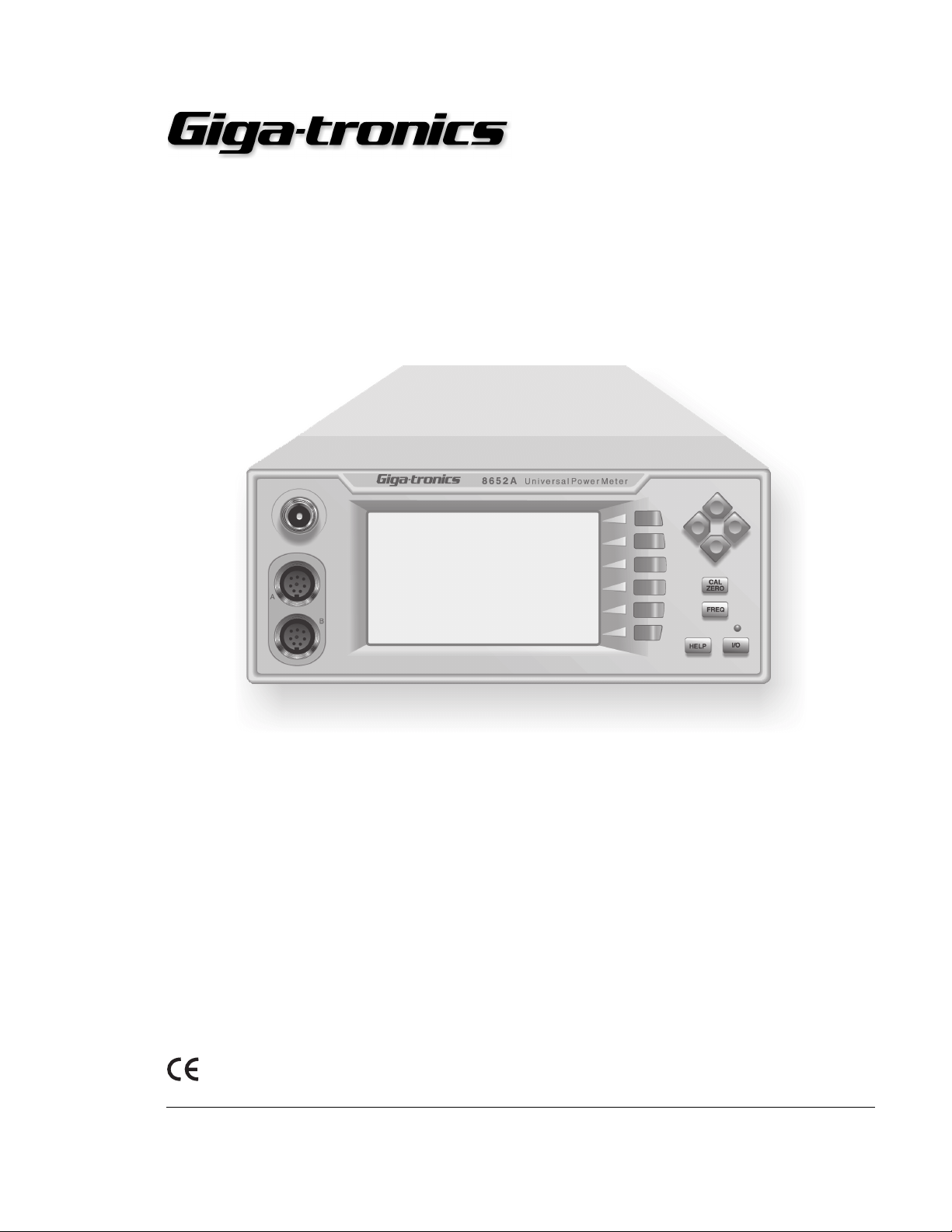
1.2.2 Line Voltage and Fuse Selection

The instrument is shipped in an operational condition and no special installation procedures are
required except to check and/or set the operating voltage and fuse selection as described in the
following.

When the instrument is shipped from the factory, it is set for a power line voltage (120 Vac for domestic
destinations). The power line fuse for this setting is 0.50 A Slo-Blo. If the source voltage is to be 220 to
240 Vac, the fuse must be changed to 0.35 A Slo-Blo (see Figure 1-1).

1

1

VOLTAGE
SELECTION
WHEEL

COVER

FUSE AND
FUSE HOLDER

0

1

2

0

Introduction

AC POWER
INPUT

Figure 1-1: AC Power Connector & Fuse Housing

The voltage selector and fuse holder are both contained in the covered housing directly above the AC
power connector on the rear panel. To gain access to them, use a small screwdriver or similar tool to
snap open the cover and proceed as follows:

1. To change the voltage setting:

Use the same tool to remove the voltage selector (a small barrel-shaped component marked
with voltage settings). Rotate the selector so that the desired voltage faces outward and replace
the selector back in its slot. Close the housing cover; the appropriate voltage should be visible
through the window (see Figure 1-1).

2. To replace the fuse:

Pull out the small drawer on the right side of the housing (marked with an arrow) and remove
the old fuse. Replace with a new fuse, insert the drawer and close the housing cover
(see Figure 1-1).

1.2.3 Power Sensor Precautions

Power sensor safety precautions, selection, specifications, and calibration are detailed in Appendix B to
this manual.

Manual 31470, Rev. E, April 2001 1-5

Series 8650A Universal Power Meters

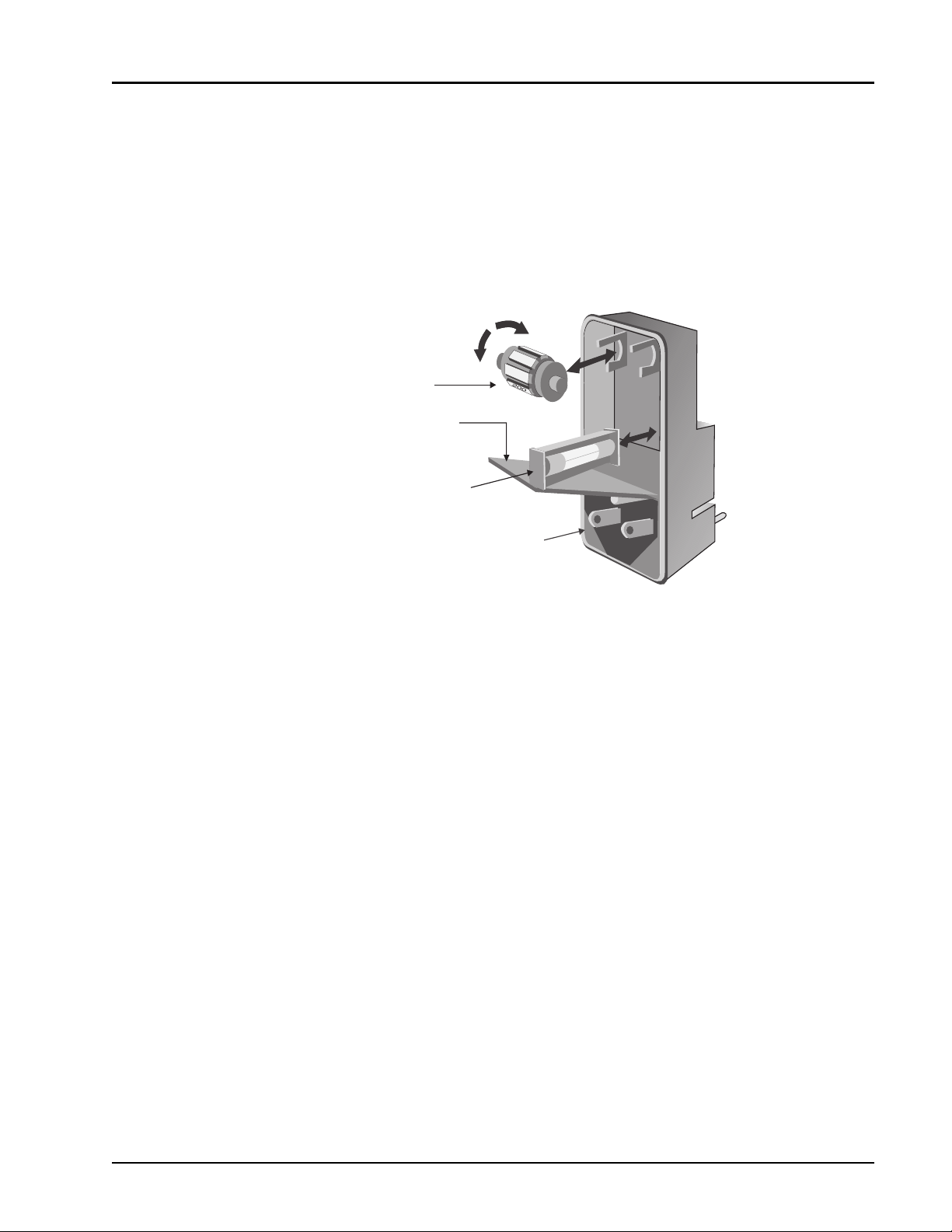
1.2.4 The Rear Panel

The rear panels for the Models 8651A and 8652A are identical and are illustrated in Figure 1-2. Any
options that have been installed in the unit will be noted on the serial number tag. Refer to the Special
Configurations section in the preface of this manual for detailed information about installed options or
other special configurations. Appendix C contains information on all available options for the 8650A.

U.S.Patent 4,794,325

!

WARNING

For continued fire protection
replace fuse with same
type and rating

WARNING

No operator serviceable parts
inside. Refer servicing to
service trained personnel

OPTION 01

Fuse

110-120V

T250 .50A

220-240V

T250 .35A

-- Line

25VA
MAX

LINE VOLTAGE

SELECTION

120Vac

Analog

Out A

GPIB

Analog

Out B

Trigger

RS-232

.

Input

Cal

V

F

In

∞

A

B

Figure 1-2: The 8650A Rear Panel

Line Voltage Selection and Fuse

Select the correct operating voltage and install the proper fuse in this housing. Refer to Section 1.2.2 for
instructions and precautions on how to select the voltage and replace the fuse.

Inputs/Outputs

Four BNC-type connectors interface the 8650A to other equipment

Trigger Input

•

accepts a TTL input for triggering and gating measurements as defined by the

Gate/Trigger menu selections, or under GPIB control. Maximum input without damage is 15 V.

V

•

PROP

accepts a voltage input that is proportional to frequency and causes the 8650A to

F In

apply appropriate frequency-related cal factors. Maximum input without damage is 15 V.

Analog Out A and Analog Out B

•

each provide an output voltage that is proportional to

the measured power level of the respective sensors connected to the front panel.

NOTE:

☛☛☛☛

8651A) or Option 04 (Model 8652A) is installed. The Sense In and the Calibrator Out

The Sense In connectors will be relocated to the rear panel when Option 03 (Model

connectors will be relocated to the rear panel when Option 13 (Model 8651A) or Option 14
(Model 8652A) is installed (descriptions of these options are in Appendix C).

Remote Interface

•

•

1-6 Manual 31470, Rev. E, April 2001

is a DB-24 connector to interface the 8650A to a host computer over the GPIB.

GPIB
RS-232

is a DB-9 connector for interfacing the meter with serial communication equipment.

1.3 8650A System Specifications

Power Meter

Introduction

Frequency Range:

Power Range:

Single Senso r

Dynamic Range:

CW Power Sensors: 90 dB

Peak Power Sensors: 40 dB Peak, 50 dB CW

Modulation Sensors: 87 dB CW; 80 dB MAP/PAP; 60 dB BAP

Display Resolution:

Measurement Modes:

Averaging:

dB Rel and Offset:

Configuration Storage

Registers:

Power Measurements and

Display Configuration:

10 MHz to 40 GHz

-70 dBm to +47 dBm (100 pW to 50 Watt)

1

User-selective from 1 dB to 0.001 dB in Log mode and from 1 to

4 digits of display resolution in Linear mode.

CW, Peak, MAP, BAP, PAP

User-selective auto-averaging or manual, 1 to 512 readings.

Timed averaging from 20 ms to 20 seconds. Automatic noise
compensation in auto-averaging mode.

Allows both relative and offset readings. Power display can be

offset by -99.999 dB to +99.999 dB to account for external loss/
gain.

Up to 20 front panel setups plus a last instrument state at power-

down to be stored and recalled from non-volatile memory.

Any four of the following channel configurations simultaneously:
A, B, A/B, B/A, A-B, B-A, DLYA, DLYB, Min/Max, Bar Graph/
Peaking Meter, Peak Hold, Crest Factor, or Mean & Std
Deviation. Alternately, full-screen graphic display of Histogram,
Strip Chart, Cumulative Distribution Function (CDF) and
Complementary CDF (CCDF) functions.

1

1

Sampling:

CW Mode and Modulation

Mode: 2.5 to 5.0 Mhz, asynchronous

Analog Bandwidth:

CW Mode:

Modulation Mode: >10 MHz

Manual 31470, Rev. E, April 2001 1-7

≥

3 kHz

Series 8650A Universal Power Meters

Time Gated Measurements:

Gate Polarity: Specifies the external signal TTL high or low level as true for

Trigger Delay: 0 to 327 ms

Gate Time: 10

Holdoff Time: 0 to 327 ms

External Trigger Polarity: Positive or negative leading edge

Delay & Range Accuracy: +1.5

Settability: 5

Trigger Signal: Standard TTL levels

defining the gated time.

µ

s to 327 ms

µ

s or 100 ppm of the set time, whichever is greater

µ

s steps or selective by cursoring to specific digits

Accuracy

50 MHz Calibrator

Calibrator: +20 to -30 dBm power sweep calibration signal to dynamically

Frequency: 50 MHz nominal

0.0dBm Accuracy: ±1.2% worst case for one year over a temperature range of 5 to

VSWR: <1.05 (Return Loss >33 dB) @ 0 dBm

Connector: Type N, 50

Standard

linearize the sensors.

35 °C.

Ω

1 GHz Calibrator

(Option 12)

Calibrator: +20 to -30 dBm power sweep calibration signal to dynamically

Frequency: 1 GHz, nominal

0.0dBm Accuracy: ± 1.2% worst case for one year over a temperature range of 5 to

Connector: Type N, 50

800 MHz to 1 GHz

Synthesizer (Option 12)

Power Range: +15 to -30 dBm, settable in 1 dB steps

Frequency: 800 MHz to 1 GHz, settable in 1 MHz steps

Power Stability: <0.1 dB/hour

Frequency Accuracy: ±0.05%

☛☛☛☛

NOTE:

0 dBm.

Power accuracy for Option 12 is only guaranteed while in calibration mode at 1 GHz,

Required for 80701A Series Sensors (see Option 12 in
Appendix C).

linearize the sensors.

35 °C.

VSWR: <1.07 (Return Loss >30 dB) @ 0 dBm

Ω

1-8 Manual 31470, Rev. E, April 2001

Instrumentation Linearity

3

2

1

0

-1

-2

-3

80301A
80310A
80320A
80321A
80322A
80325A
80330A

80401A,80601A (CW)

80701 (CW)

-70

-64

-60

-50

-40

-40

-30

-67

-64

-60

-54

-50

-40

-30

-30

-20

-57

-54

-50

-44

-40

-30

-20

-20

-10

-47

-44

-40

-34

-30

-20

-10

-10
0

-37

-34

-30

-24

-20

-10
0
0

10

-27

-25

-20

-14

-10
0
0

10
20

-17

-16

-10

-4
0

10
20
20

-7

-7

0

6
10
20
20
30

3

3

10
16
20
30
40
40

13
13

20
26
30
40
44
50

20
20

Input (dBM)

SENSORS

Typical Error (dB)

System Linearity at 50 MHz: ±0.02 dB over any 20 dB range from -70 to +16 dBm

±0.02 dB (±.05 dB/dB) from +16 to +20 dBm
±0.04 dB from -70 to +16 dBm

The following chart shows linearity plus worst case zero set and

noise vs. input power.

Introduction

1

Temperature Coefficient of

Linearity: <0.3%/ °C temperature change following Power Sweep

calibration. 24-hour warm-up required.

Zeroing Accuracy: (CW)

Zero Set: <±50 pW, <± 100 pW with 80400A, 80600A series Modulation

Power Sensors.
<±200 pW with 80700A Series Sensors.

<±100 pW during 1 hour

Zero Drift (during 1 hour): <±200 pW with 80400A and 80600A Series Modulation Sensors

<±400 pW with 80700A Series Sensors

Noise: <±50 pW, <±100 pW with 80400A and 80600A Series

modulation power sensors.
<±200 pW with 80700A Series Sensors.
Measurable over any 1 minute interval after zeroing, three
standard deviations.

Notes:

1. Depending on sensor used (see Power Sensor details in Appendix B).

2. Zero Drift Measurement
a. Set the meters Average to 512. Perform Calibration. Connect a 50-ohm load to the sensor after Calibration and

Zero meter.

b. Temperature stabilize at 25 °C for 24 hours.
c. After the 24 hour stabilization, perform a Zero Drift test.
d. Zero the meter and take an initial measurement reading.
e. Continue taking one reading every 10 minutes until 6 readings have been taken.

Plot the 6 readings, Zero Drift should be ±200pW or ±400pW, depending on the sensor.

Manual 31470, Rev. E, April 2001 1-9

Series 8650A Universal Power Meters

Measurement Rates

Table 1-1 illustrates typical maximum measurement rates for different measurement collection modes.
The rate of measurement depends on several factors including the controller speed and the number of
averages. The Fast Buffered Mode speed does not include bus communication time. Measurement speed
increases significantly using the 8650A Fast Buffered Mode. Storing data in the power meter’s memory
for later downloading to your controller reduces GPIB protocol overhead. Up to 5000 readings can be
buffered.

Table 1-1: Measurement Rates

Measurement

Collection Mode

Normal (TR3), Continuous Single
Readings

Swift Mode, Continuous or
Buffered, Bus/TTL triggered >1750 800

Fast Buffered Mode, Buffered Data, Time
Interval = 0

Fast Modulated Mode, Continuous Single
Readings

Readings per Second

(CW Measurement)

>300 150

26,000 N/A

N/A 800

Readings per Second

(MAP, PAP, BAP

Measurement)

Individual data points are read immediately after measurement in the Normal mode. The Normal mode
and the Swift mode both slow down at low power levels (<-37 dBm for Standard Sensors) to average the
effects of noise. The Swift mode allows triggering of individual data points and can store the data in the
8650A memory. Measurement timing of individual data points is controlled by setting the time interval
(0 to 5000 ms) between the data points following a trigger.

Remote Operation

GPIB Interface: All front panel operations and some GPIB-only operations to be

Interrupts: SRQs are generated for the following conditions:

remotely programmed in IEEE 488.2 or IEC-625 formats.

Power Up, Front Panel key actuation, Operation Complete and
Illegal Command.

Fast Buffered Mode Controls

Trigger Source: TTL or GPIB

Data Buffer Control: Pre- or Post-measurement data is collected immediately either

Time Interval: TIME ### - controls time interval in milliseconds between

1-10 Manual 31470, Rev. E, April 2001

before or after receipt of the TTL or GPIB trigger.

measurements. Accurate to 5%, typical.

Inputs/Outputs

V

F Input (BNC): Recalls cal factors using source V

PROP

Introduction

F output. Corrects power
readings for sensor frequency response using sweeper voltage
output. Input resistance = 50K. Does not operate in the fast
measurement collection modes (normal mode only).

PROP

Analog Output (BNC): Provides an output voltage of 0 to 10V from either Channel A or

Trigger Input (BNC): Accepts a TTL trigger input signal for swift and fast measurement

GPIB connector: Interfaces the power meter to a host computer for remote

RS-232 connector: Interfaces the power meter to serial communications equipment,

Channel B in either Log or Lin units. Does not operate in the swift
and fast measurement buffered modes.

buffered modes, and time gating mode.

programming using SCPI, IEEE 488.2 and IEC-625 coding, also
emulation modes.

using RS-232 format.

General Specifications

Temperature Range:

Operating: 0 to 55 °C (32 to 13 2 °F)

Storage: -40° to 70 °C (-40° to 158 °F)

Power Requirements:

100/120/220/240Vac <± 100 pW 10%, 48 to 440 Hz, 20 VA

typical

Physical Characteristics:

Dimensions: 215 mm (8.4 in) wide, 89 mm (3.5 in) high, 368 mm (14.5 in)

Weight: 4.55 kg (10 lbs)

deep

Options

Refer to Appendix C for descriptions of options.

Power Sensors

See Appendix B for power sensor selection, specifications and calibration data.

Manual 31470, Rev. E, April 2001 1-11

Series 8650A Universal Power Meters

1-12 Manual 31470, Rev. E, April 2001

2.1 Introduction

This chapter describes how to operate the Series 8650A Universal Power Meter using the display and
controls on the front panel. It includes descriptions of the front and rear panels, configuration, display
menus and practical applications.

See Chapter 3 for instructions for remote operation of the 8650A over the General Purpose Interface
Bus (GPIB) and RS-232 serial communication devices.

2.1.1 The Front Panel

Although the 8650A has different modes of operation, the front panel is simple in design and easy to
use. The instrument is configured and controlled by means of the dedicated hardkeys and the display
menus, which are accessed and controlled with the data interaction softkeys.

The dual-channel Model 8652A front panel is illustrated in Figure 2-1. The single-channel Model
8651A is the same in appearance but does not include the Sensor B connector.

2

Front Panel Operation

Figure 2-1: The 8652A Front Panel

Manual 31470, Rev. E, April 2001 2-1

Series 8650A Universal Power Meters

Dedicated Hardkeys

The dedicated hardkeys are located on the right side of the front panel and function as described below.
In this manual, instructions to press a dedicated hardkey are with the appropriate key title in bold
uppercase enclosed in brackets, such as ‘press

Cursor Keys:

These four keys are arranged in a diamond pattern and move the highlighted item (cursor) in the
display to the desired location. A small diamond symbolizing the cursor keys appears in menus, with
an arrow in the keys that are effective for that menu. If more than one field is highlighted, the cur­sor pattern will be located nearest the one that will be activated when the cursor keys are pressed.

CAL/ZERO:

This key is for zeroing and calibration of a power sensor. All active sensors should be zeroed when­ever any sensor is added or removed, whether it is calibrated or not.

FREQ:

This key specifies the frequency of an input signal so that the power meter can apply the frequency­specific cal factor from the sensor EEPROM to the measurement.

[CAL/ZERO]

to calibrate a power sensor’.

If the frequency of the input signal changes so often that it is impractical to keep entering the fre­quency with the FREQ key, the frequency information can be conveyed to the 8650A by the use of
a voltage input that is proportional to frequency (see the V

F connector on the rear panel).

PROP

When the 8650A is controlled remotely over the GPIB, the frequency information can be sent over
the bus.

HELP:

Help screens describe the current display and present your options. From any menu, press

[HELP]

to display the associated Help screen. Press the up or down cursor key, if shown, to scroll the help
screen up or down one line at a time. Press [Exit Help] to leave the Help screen and return to the
current menu.

Power:

This push-push switch turns main power on and off. The LED above the power switch will be green
when the unit is ON, and will turn yellow indicating the standby mode when the power switch is
OFF with the main ac power still connected. The LED will be OFF when the ac power is discon­nected. All user setting and sensor calibrations will be automatically stored in non-volatile memory
for recall when ac power is turned off with the front panel on/off switch.

CAUTION

To avoid losing some current settings and ensuring that the meter
powers up properly, observe the following procedures:

1.) Remove AC Power to the rear panel only after at least 1 second has lapsed from the time the
front panel ON/OFF switch has been pressed to turn off the meter.

2-2 Manual 31470, Rev. E, April 2001

Front Panel Operation

2.) Cycling the ON/OFF switch should be no faster than once a second. Pressing the ON/OFF
switch in rapid succession is not recommended.

3.) If the current setup is critical, it is recommended to save it as a stored setup to prevent
accidental loss.

Display Screen

The liquid crystal screen displays measurements and configuration data. It also displays the operating
and control functions that can be selected with the data interaction softkeys. Figure 2-1 illustrates a
typical display screen with the menu control functions aligned with the data interaction softkeys.

The menus to calibrate and perform measurements with the 8650A are many and varied. A complete
menu map is provided in Appendix D of this manual. Until you are thoroughly familiar with the
operation of the 8650A, referring to the appropriate menu map to reach the function you intend to
perform should speed up your operation.

When you turn on the power the model number and software version will display for five seconds and
then be replaced with the Main display (see Figure 2-2).

Data Interaction Softkeys

The data interaction softkeys select the options for configuration and measurement control. In this
manual, instructions to press a softkey are identified with the selected option in italics enclosed in
brackets, such as ‘press [Sensor Setup] to configure a new power sensor’. Softkey statements will be in the
same case as in the actual displays.

Sensor Inputs

and B connectors interface Channel A and Channel B sensors to the power meter. Dual-

AAAA

The
channel Model 8652A has A and B sensor inputs; single-channel Model 8651A has only sensor A
input. Refer to the Sensor Configuration details in Section 2.2.4.

CAUTION

When connecting sensor cables to these inputs, the cable pins
must be aligned properly. Orient the cable so that the guide on the
end of it aligns with the notch on the sensor input. If the connec­tor does not seem to fit, forcing it will only damage the connector
pins.

Calibrator Output

The Calibrator connector is a reference power output for calibrating the amplitude response of a power
sensor (see Section 2.3.3 for instructions on how to calibrate and zero sensors). The frequency of the
output is fixed at 50 MHz or 1 GHz, depending on the sensor in use. The Calibrator output can also be
used as a programmable low-level power output (see Section 2.2.1). During a calibration run, the output
level automatically sweeps from -30 dBm to +20 dBm in 1-dB steps.

Manual 31470, Rev. E, April 2001 2-3

Series 8650A Universal Power Meters

2.2 8650A Configuration

The 8650A screen normally displays measurement data, but it also displays the setup and configuration
menus for the meter, display, and sensor. The setup menus are dynamic; the display adapts to the current
operating mode and the type of sensors and other peripheral connections. For example, the sensor
identification in Figure 2-2 will display only when a sensor is connected. If a sensor is not connected,
the menu will indicate ‘No Sensor A’. The menu displays these other peripheral data only when
applicable.

Figure 2-2 illustrates the Main Menu; other screens will display when sensors are connected or removed.
Note that this is the only display that does not contain a mode or identification title in reverse video
across the top of the screen.

The options available from the Main menu are:

• Meter Setup for configuring the meter (see Section 2.2.1)

• Display Setup for configuring the display (see Section 2.2.2)

• Sensor Setup for configuring installed sensors (see Section 2.2.4)

• dB/mW for selecting dB or power as the measurement unit (see below)

• Reset Menu to refresh a min/max value (see below)

• Rel for recording Relative Measurements (see Section 2.2.3)

CAL ON

A - 46.01

B - 50.52

A/B
A

From the Main Menu, press [dB/mW] at any time to toggle between dB and mW as the measurement
units. The values on the displayed lines will also change to match the units.

The Main Menu will display a Reset Menu selection only after you have configured one or more lines to
display the data gathering functions, such as Min/Max (illustrated in line 4 in Figure 2-2), Bar Graph/
Peaking Meter, Peak Hold, Crest Factor, and Mean & Standard Deviation. When the selection is
displayed, press [Reset Menu] to reset the accumulated data to it’s current value. Refer to Section 2.2.2
for detailed instructions on how to configure the display lines.

Most screens contain ‘OK’ and ‘Cancel’ options. After you have entered changes into the display, press
[OK] to store the changes (this equates to Enter on a keyboard), or [Cancel] to cancel and return to the
previous display without storing any changes (this equates to Escape on a keyboard).

- 4.49

-Min -45.95 dBm

-Max -46.04 dBm

Figure 2-2: The Main Menu

CW
dB

CW
dBm

dBm

MAP

Rel

dB

mW

Reset

Menu

Sensor

Setup

Display

Setup

Meter

Setup

2-4 Manual 31470, Rev. E, April 2001

2.2.1 Meter Setup

The Meter Setup menu provides the means to configure the meter operating mode, and to store and
recall setups. From the Main menu, press [Meter Setup] to display the Setup Menu. Press the softkey for
the function you want to perform. The options are:

• Calibrator to Configure and to turn the Calibrator output ON or OFF

• Config to configure the operating mode and parameters

• Sto/Rcl to store and recall meter setups

• Service to clear all memory (additional service routines may be added to future revisions of this
product)

• Display Return to return to the Main menu without selecting a configuration option

Calibrator

The procedures in this section describe only how to use the Calibrator output as an RF output; see
Section 2.3.3 for procedures to zero and calibrate power sensors. The Calibrator function must be turned
ON to use the output as an RF source, indicated by the words
Main Menu (see Figure 2-2).

Turn on the 8650A for 15 minutes then cycle the power OFF and ON, this establishes the 1 mW
reference for the instrument firmware.

Front Panel Operation

CAL ON

in the upper left corner of the

To turn the Calibrator ON or OFF, press [Meter Setup] from the Main Menu. This will display the Setup
Menu. From the Setup Menu, press [Calibrator] to display the Calibrator menu. Toggle the Calibrator
On or OFF by pressing [On/Off].

☛☛☛☛

1. Press [Level dBm] to set the RF output level in dBm. Enter the level with the cursor keys.

2. Press [Level mW] to set the RF output level in power. Enter the level with the cursor keys.

3. Press [Frequency] to set the output reference frequency. Enter the frequency with the cursor keys.

4. Press [OK] to accept the changes or [Cancel] to cancel the changes, and return to the Power Meter

NOTE:

displayed, but it will be changed to reflect your selection when you return to the Main
Menu.

Frequencies other than 50 MHz are available only with Option 12 (see Appendix C).

Configuration menu.

The wording at the top of the screen will not change while this menu is

Manual 31470, Rev. E, April 2001 2-5

Series 8650A Universal Power Meters

Config

Press [Config] from the Setup menu to display the Power Meter Configuration menu (see Figure 2-3).
From this menu you can configure the following:

• GPIB mode and address

•V/F (V

• Analog A and B outputs

• RS-232 interface

• Time Gate trigger mode and time parameters

• Strip Chart graphic display

• Histogram graphic display

• Sound

F) input frequency and scale factor

PROP

Power Meter Configuration

GPIB

V/F In

Analog Out A

Strip Chart

Sound

Mode: 8600 Addr: 13

Figure 2-3: Power Meter Configuration Display

RS-232

T-Gate

Analog Out B

Histogram

OK

Config

Cancel

Select the item to be configured with the cursor keys, then press [Config]. The following options will be
available for configuring the power meter:

GPIB:

This option assigns the GPIB protocols and address for control of the 8650A over the GPIB interface.

1. From the Power Meter Configuration menu, move the cursor to the GPIB field and press [Config].
The menu to set the GPIB mode and address will display.

2. Press [Mode] to highlight the operating mode and use the cursor keys to select the desired mode of
operation. The options are:

• SCPI to use the SCPI IEEE 488 command set

• 8600 to use the IEEE 488.2 8650 native mode

• 8542 to use the dual-channel 8542 emulation mode (Model 8652A only)

• 8541 to use the single-channel 8541 emulation mode

• 438A to use the HP-438A emulation mode

• 437A to use the HP-437A emulation mode

• 436B to use the HP-436B emulation mode

3. Press [Address] to move the cursor to the Address field. Step the address value up and down with the
cursor keys. Valid addresses are:

• 00 through 30 in the Listen & Talk mode

• 40 in the Listen-Only mode

• 50 in the Talk-Only mode.

2-6 Manual 31470, Rev. E, April 2001

Front Panel Operation

4. Press [OK] to accept the changes or [Cancel] to cancel the changes and return to the Power Meter
Configuration menu.

V/F In:

The V/F (V

F) input accepts a frequency referenced to 0 Vdc, which the power meter uses to

PROP

determine and apply the appropriate correction factors (stored in the sensor EEPROM). The voltage
input is supplied by a V/GHz output from the signal source. Two values must be defined for V

PROP

F: the
frequency at 0 Volts, specified in Hz, MHz or GHz, and the scale factor specified in V/GHz. The V/GHz
output connector on the frequency source is usually labeled with the scale factor.

From the Power Meter Configuration menu, move the cursor to the V/F In field and press [Config]. The
V/F Config menu will display.

1. Frequency:

a. Press [Zero] to highlight the first digit of the frequency.

b. Press the up/down cursor keys to select the value of the first digit of the frequency.

c. Continue in the same manner to set all of the digits for the desired frequency. The units adjust

automatically as you enter the frequency.

2. Scale:

a. Set the scale factor by pressing [Scale] and setting the value in the same manner described for

the frequency.

b. Press [OK] to accept the changes or [Cancel] to cancel the changes, and return to the Power

Meter Configuration menu.

Analog Out A and Analog Out B:

The Analog A and B outputs are voltage proportional to measured power that can be applied to
auxiliary test equipment such as a data recorder.

1. Select Source:

The choices of output source are Line 1 through Line 4. The configuration of the Analog outputs is
interactive with the Display Configuration. If any line is set for accumulated data, such as Min/
Max, PKHold, CrFact, or Mean & Std Dev, it will not be displayed here for configuration.

2. Log/Lin:

The mode choices are Log and Linear. Press [Log/Lin] to toggle between the Log and Linear modes.

3. Set Scale:

The Set Scale menu adds the options to set the High and Low range in values of volts and power.
Press [Set Scale] to enter this menu.

a. Press [Set High] to select the High range or [Set Low] to select the low range.

b. Press [Power] or [Volts] to toggle between the volts and power values.

Manual 31470, Rev. E, April 2001 2-7

Series 8650A Universal Power Meters

c. Use the cursor keys to set the desired value in either the High or Low range.

d. Press [Set Volts/Set Power] to toggle between each value. Set the digit value of each with the

cursor keys.

e. Press [OK] to accept the changes or [Cancel] to cancel the changes and return to the Power

Meter Configuration menu.

Strip Chart

The Strip Chart function plots measurements on the screen over a fixed period or continuously. The
X-axis displays time from the start of a measurement to a selective period of 1 to 200 minutes. While
running, the adaptive autoscaled high and low plotting limits are displayed. While paused, the cursor
can be used to review plotted values.

1. From the Power Meter Configuration menu, move the cursor to the

Strip Chart

field and press

[Config] (see Figure 2-4).

2. Press [Select Source]. The choices for measuring sources are Lines 1 through 4. If any line is set for
data gathering, it will not be displayed here.

3. Press [Sample Rate]. The choices are from 1 sample per minute to 5 samples per second.

4. Toggle between [Hold Bfr] to stop sampling when the buffer is full, or [Rot Bfr] to set the Strip Chart
display to update continuously with new samples after the buffer is initially full while discarding the
same number of beginning samples.

5. Press [OK] to accept the changes or [Cancel] to cancel the changes, and return to the Power Meter
Configuration menu.

CAL ON

-7

-27

STRIP CHART

Reset

Run

Pause

Cur on

Cur off

-15.75 dBm 33.5 sec (crsr)

A

Figure 2-4: Illustration of the Strip Chart

Exit

Sound:

A speaker within the chassis produces audible clicks and tones to register keystrokes and to draw
attention to certain conditions. For example, if a limit has been exceeded or a calibration process has
been completed. Press [On] to enable the speaker, or [Off] to disable it. There is no sub menu associated
with this feature.

2-8 Manual 31470, Rev. E, April 2001

Front Panel Operation

RS-232:

Highlight the RS-232 option in the Power Meter Configuration menu and press [Config]. The RS-232
Config menu will display for configuration of the RS-232 interface.

1. Press [Baud] to set the Baud Rate. Select the desired rate with the up/down cursor keys. The default
value is 9600.

2. Press [Length] to set the Data Bits. Select the desired data bit length with the up/down cursor keys.
The default value is Press [Parity] and turn the parity on or off with the up/down cursor keys. Default
parity is off.

3. Press [Stop bits] to set the stop bit value. Select the desired stop bit value with the up/down cursor
keys. The default value is 1.

4. Press [OK] to accept the changes or [Cancel] to cancel the changes and return to the Power Meter
Configuration menu.

T Gate:

The Time Gate mode supplies a digital control voltage to enable or disable readings from any one or all
sensors. Thus, the mode limits a power measurement to a defined interval that is controlled by a start
time and a duration. The start time begins after a programmable delay following an external or internal
trigger.

☛☛☛☛

NOTE:

The Time Gate feature operates only with modulation sensors.

Figure 2-5 illustrates the time gated measurement with an external time gated pulse applied to the
trigger input. In this mode, the time gate starts and ends with the input of a high or low TTL level input.
The duration of the measurement corresponds to the duration of the gated pulse.

RF RF

Ext Gating
(TTL = High)

Gate
Time

Ext Gating
(TTL = Low)

Gate
Time

Figure 2-5: Illustration of External Gating

Manual 31470, Rev. E, April 2001 2-9

Series 8650A Universal Power Meters

Proceed as follows to configure the power meter for gated measurements by the sensors:

1. From the Power Meter Configuration menu, select [T Gate] then [Config] to display the Gate/
Trigger menu.

2. From the Gate/Trigger menu, select the sensor with the cursor keys, then select the mode of gated
operation for that sensor. The options are External Gate, Ext. Trigger Rising, External Trigger
Falling, and Burst Edge.

a. Gate:

This configures the gate to measure only during a high or low input. Gate Low enables power
meter readings on a low logic input, and Gate High enables readings on a high (+5 V) logic
voltage input (see Figure 2-5).

1.) Select the sensor to be configured with the cursor keys. The current configuration of
the selected sensor will be indicated in the window at the bottom of the screen.

2.) Press [External Gate] to set the sensor gate measurement to high or low.

3.) Press [Gate High] or [Gate Low] to set the external gating to a high or low logic state.

4.) Press [OK] to return to the Gate/Trigger menu, or <Cancel> to abort the
configuration.

b. External Trigger:

Figure 2-6 illustrates the Time Gated measurement parameters with an external trigger. When
an external trigger is input (point A in Figure 2-6), it starts the Trigger Delay. At the end of the
Trigger Delay, the Gated Time measurement starts and lasts until its preselected time expires.
The Holdoff Time then prevents any further trigger inputs (such as point B below): from start­ing a new gated measurement until it has timed out.:

Holdout

Time

B

RF

EXT TRIG

A

Trig

Delay

Gate
Time

Figure 2-6: Illustration of External Triggering

1.) Press [Ext Trigger Rising] or [Ext Trigger Falling] to set the parameters of the external
trigger. The settings are:

✔ Delay

✔ Gate Time

✔ Holdoff

2-10 Manual 31470, Rev. E, April 2001

Front Panel Operation

Upon entering the External Trigger setup, a burst profile will display at the bottom
of the screen. If the following specifications are not met, the profile may be inaccu­rate or not displayed at all:

a.) The time from between trigger edges is the period of the trigger. The period

must be equal to or less than 50 ms.

b.) The burst must be at least 0.1 ms wide and have at least 0.1ms off time.

c.) The trigger edge must occur before the leading edge of the burst.

d.) The points on the profile represent a resolution in time, which will vary

according to the requirement that the burst fit on the screen, to a minimum
of approximately 10 µs per displayed point.

µ

2.) Set the value of the delay with the cursor keys. The range is 0

µ

3.) Select [Gate Time] and set its value. The range is 5

4.) Select [Holdoff] and set its value. The range is 0

5.) Press [OK] to accept the changes or [Cancel] to cancel the changes and return to
the Power Meter Configuration menu.

s to 327.625ms.

µ

s to 327.625ms.

s to 327.625ms.

c. Burst Edge:

The Burst Edge mode uses the burst edges detected by the sensor to trigger power measure­ments, and is configured essentially the same as External Triggering described above. The setup
screen for this mode also displays a burst graphic profile with the same conditions as described
for External Triggering.

1.) Set the Delay and Gate time as described for External Trigger in steps 2) and 3)
above.

2.) Press [OK] to accept the changes or [Cancel] to cancel the changes, and return to
the Power Meter Configuration menu.

OK

Delay

Gate

Time

Numeric

Graphic

Cancel

Delay

Gate Time:

Burst Edge

0.070 ms

0.400 ms

Figure 2-7: Illustration of Burst Edge Configuration

Manual 31470, Rev. E, April 2001 2-11

Series 8650A Universal Power Meters

Histogram

The Histogram feature displays graphical views of accumulated data distribution over a selective period
of time (see Figure 2-8). Highlight the Histogram option in the Power Meter Configuration menu and
press [Config].

1. Press [Select Source] and select the input channel (8652A only) or display the line number.

2. Toggle Log or Lin with the [Log/Lin] softkey.

3. Press [Interval] and select the duration the data is to be acquired. The range is from 1 second to 96
hours, or continuous.

4. Press [OK] to accept these settings or press [Cancel] to cancel the settings, and return to the Power
Meter Configuration menu.

5. Press [OK] from the Power Meter Configuration menu. The Histogram will display full screen as
shown in Figure 2-8.

CAL ON

-48.62 dBm -43.62 dBm
Cursor: - 46.89 dBm 1.45%

Interval: 1 min (sampling complete)

Sensor A Histogram

2%

0%

Figure 2-8: Illustration of the Histogram

Reset

Select

Mode

Vert

Horiz

Zoom

Zoom

Out

Exit

In

There are additional functions available from the Histogram screen:

1. Press [Reset] to restart sampling.

2. Press [Select Mode] to toggle between distribution display functions.

a. The Histogram (see Figure 2-8) shows the percentage of time each power level is measured.

b. The CDF (Cumulative Distribution Function) shows the percentage of time a signal is below a

selected power level (see Figure 2-9). The x-axis displays the power level and the y-axis displays
the percentage of time the power is at or below the power level specified by the x-axis.

c. The CCDF (Complementary CDF) (see Figure 2-10) shows the percentage of time a signal is

above a selected power level for more accustomed viewing of a descending slope.

3. Press the [Vert/Horiz] toggle key to select the zoom axis scale, then press [Zoom In] or [Zoom Out] for
the selected axis.

2-12 Manual 31470, Rev. E, April 2001

Front Panel Operation

4. Move the cursor along the slope of any curve to display, below the graph, the cursor position, the
power level and the corresponding percentage of time the signal is above or below that level.

CAL ON

-48.62 dBm -43.62 dBm
Cursor: - 46.32 dBm 44.05%

Interval: 1 min (sampling complete)

CAL ON

-48.62 dBm -42.62 dBm
Cursor: - 64.90 dBm 46.32%

Interval: 1 min (sampling complete)

Line 1 (A) CDF

Figure 2-9: Illustration of the CDF Curve

Line 1 (A) CCDF

100%

0%

100%

0%

Reset

Select

Mode

Vert

Horiz

Zoom

Zoom

Out

Exit

Reset

Select
Mode

Vert

Horiz

Zoom

Zoom

Out

Exit

In

In

Figure 2-10: Illustration of the CCDF Curve

Sto/Rcl

Up to 20 setup configurations can be stored in and recalled from non-volatile memory.

Recall:

1. From the Setup Menu press [Sto/Rcl].

2. Select [Recall] to recall a previously stored setup.

3. Step through the stored setup addresses with the cursor keys until the setup to recall is
displayed.

4. Press [OK] to recall the selected setup.

5. Press [Recall Preset] to recall the default setup for the connected sensors.

Store:

1. To store the current configuration, press [Sto/Rcl] from the Setup Menu.

2. Select [Store] to store the current setup.

3. Select the setup ID (1 through 20) that you want to assign to this setup.

Manual 31470, Rev. E, April 2001 2-13

Series 8650A Universal Power Meters

4. A name of up to 16 characters can be used as an additional means of identifying the setup. Press
[Name} to open the display containing this option. Set the name by moving the cursor to the
first position desired with the < and > softkeys, then select the character for that position with
the cursor keys. Repeat this process for each character in the name.

5. Press [OK] to accept the stored data or press [Cancel] TWICE to cancel the changes, and return
to the Power Meter Configuration menu.

Service

This is presently used only to clear all memory in the 8650A. When you press [Service], you will be
prompted to press [Clear Mem] to clear all calibration, configuration, and measurement data currently
stored in the 8650A RAM. Data stored in sensor EEPROMs are not affected.

2.2.2 Display Setup

Use this option to configure the data and format that will display on each line of the screen.

From the Main Menu, press [Display Setup] to select the Configure Display menu (see Figure 2-11). This
screen is the same as the Main Menu except the control items are changed to display line configuration
options. The configuration of each line includes the source and data format, data resolution, and
peaking meter (bar graph) when configuration for use. In addition, the control to set the screen
brightness is included in this display (Other Options).

One to four lines of data can be configured, and any attached sensor can be mapped to any of the four
lines. Other information items are displayed at the top of the screen. These include

,

displays whenever the calibration RF source is on;
meter is being operated by remote control (GPIB or RS-232); and configured inputs

B/A

☛☛☛☛

and

.

B-A

NOTE:

channel Model 8651A will have input A only.

The above input configurations are available only in the Model 8652A. The single-

CAL ON

Configure Display

A - 70.999

B - 54.245

A/B

A

- 16.754

-B

-24.246

Figure 2-11: The Configuration Display Menu

REMOTE

CW
dB

CW
dBm

dB

CW
dBm

which displays whenever the power

Line 1

Line 2

Line 3

Line 4

More

Options

Cancel

CAL ON

A, B, A/B, A-B,

, which

2-14 Manual 31470, Rev. E, April 2001

Front Panel Operation

Line Configuration

Select the line to be configured by pressing the corresponding [Line n] softkey. The menu in Figure 2-12
will display. The current configuration of the selected source displays in the large window at the bottom
of the screen.

Data Line 1 Configuration

Source

A B

Line 2 3 4
Other

Off

A 11.11

Figure 2-12: The Data Line Configuration Menu

Data

A A/B

A-B

Statistics

CW
dBm

OK

Select

Source

Select

Data

dB

mW

Config

Cancel

Source:

1. Press [Select Source] to enable the cursor in the Source field.

2. Move the highlight with the cursor keys to select the desired source.

a. A B:

This corresponds to sensor A and B inputs. The Data field will show the line configuration
possibilities when you select the corresponding source input. When you select source
Data field will read

B, B/A

and

B-A

A, A/B

.

and

. When you select source B, the Data field will read

A-B

A-B

A-BA-B

A

, the

b. Line n

:

When you select Line n in the Source field, the Data field will change to

Min/Max

. You
will be configuring the selected line number to be the source. For example, you can use the
selected line to display the minimum/maximum values of another line (Line n). The only
line numbers that will be available for selection are those which have already been config­ured and are not configured to show min/max values of other lines. If you want the
selected line number to show the min/max values of another line but the line is not avail­able in the source list, you will have to go back and reconfigure the missing line. It may not
be configured at all, or it may be configured to display the min/max of another line.

c. Other:

This selection changes the Data field to copy another line into the line number you are
configuring. The Data field will change to indicate the lines, such as n1—>n2, meaning
that line n1 will be copied into line n2 (the line you are configuring). You will find this
option useful, for example, if you want to change a line but do not want to lose its configu­ration; you can select Other and copy the configuration to a different line and retain the
configuration on the new line.

Manual 31470, Rev. E, April 2001 2-15

Series 8650A Universal Power Meters

d. Off:

Select this option to turn the line off. When a line is turned off, it will not be available as
a source Line n. For example, if Line 4 is turned off, you cannot set Line 3 to read the min­imum/maximum values of line 4.

Data:

1. After you have selected the source for the line being configured, press [Select Data] to enable
the cursor in the Data field.

2. Move the highlight with the cursor keys to the configuration of your choice.

a. When you select source

, the Data field will read B,

B

source

, the Data field will read A,

A

and

B/A

B-A

.

A/B

and

. When you select

A-B

b. Other measurements that can be selected for Modulation Sensors are Peak Hold, Crest

Factor, and Mean & Standard Deviation.

3. DB/mW:

This selection toggles the line units between dB and mW. It can be changed at any time to dis­play the opposite units.

Config:

Use the Config selection to set the measurement resolution, upper and lower limits, and utilization
of the bar graph. Lines configured with Statistics can be configured only for resolution; the Set Limits
and Bar Graph options will not display for these lines.

1. Press [Config] and use the cursor keys to set the resolution of the input. The resolution will be
displayed in the large window at the bottom of the screen. Adjust the resolution with the
cursor keys to the desired level. The range is 0 to 3 decimal places.

2. Press [Set Limits] to set the upper and lower measurement limits, or to turn the limits off.

a. Press [High] and set each digit of the high limit with the cursor keys.

b. Press [Low] and set each digit of the low limit with the cursor keys.

c. Press [Limits Off] to disable use of the limits. Press [High] or [Low] again to enable and set

the limits.

3. Press [Bar Graph] to set the utilization of the bar graph scale.

a. The menu will display as described above for Set Limits.

b. Follow the Set Limits procedure above to set the bar graph scale, or to disable the bar graph.

c. The upper and lower limits of the bar graph will be displayed in the Main menu as brackets

with the current measurement shown as a horizontal bar between the brackets (e.g.,[ ]).

4. Press [OK] to save all changes and return to the Configure Display screen, or [Cancel] to leave
the configuration without saving any changes.

2-16 Manual 31470, Rev. E, April 2001

More Options

1. Select [More Options] from the Configure Display menu (see Figure 2-11) to set the brightness of
the display screen. The adjustment, made with the cursor keys, is interactive so you can observe the
brightness as you adjust it. The range is 0% (off) to 100%. The default is 70%.

2. Press [OK] to save all changes and return to the Configure Display screen, or [Cancel] to leave the
configuration without saving any changes.

2.2.3 Rel

Normally, each line of the display shows a sensor measurement value. When you press [Rel] from the
Main menu, the present measured value of each line is recorded and all subsequent measurements are
expressed in dB or percentage relative to that recorded value. The Relative Measurement menu provides
a means of selectively enabling or disabling the relative measurement mode for channels A or B.

Press [Select Line] repeatedly to select the line to be used for relative measurements. Use the cursor keys
in this menu only to change the value of the selected line.

The selected line can be switched in and out of the Relative Mode by pressing the [Rel On/Off] key.

2.2.4 Sensor Setup

Front Panel Operation

Sensor configuration enables you to select the operating mode of sensors, or to select the parameters for
averaging time-based measurements. From the Main Menu, press [Sensor Setup] to display the installed
sensor data and configuration options (see Figure 2-13). The power meter reads the contents of the
EEPROMs for installed sensors and displays each type of sensor and its connecting input.

The [Sensor Setup] softkey will not function if there are no sensors attached, or if attached sensors have
not been calibrated. The Sensor Setup options are dependent on the type of sensor. All sensors options
are

Avg

and

Offset

. Peak and Modulation sensors add a

Sensor Setup

A: Peak Sensor

B: Modulation Sensor

First select sensor above,
Then configuration mode at right

Figure 2-13: The Sensor Setup Menu

Config

Offset

Config

Cancel

option (see Figure 2-13).

OK

Avg

Manual 31470, Rev. E, April 2001 2-17

Series 8650A Universal Power Meters

Avg

Use this option to set the averaging period of power measurements, including modulated, CW and peak
sensors. Press [Avg] from the Sensor Setup menu to display the

menu

. This menu offers three options: Auto, Averages, and Time.

:

Auto

1. Select this setup option if you want the time to be ‘adaptive’ averaged. That is, the time
window changes dynamically to reduce the effects of transient changes in power levels.

2. Press [OK] to store the changes, or [Cancel] to exit without saving changes.

Averages:

1. Select this setup option to set the number of periods for averaging measurement signals over a
fixed period of time. Each unit is approximately 20 ms in duration. You have a choice of
‘powers of two’ multiples of units from 1 to 512. Set the number of periods with the up/down
cursor keys.

2. Press [OK] to store the changes, or [Cancel] to exit without saving changes.

Sensor Setup - Averaging

Time:

1. Select this option to average measurement signals over a fixed period. A menu will display for
you to set the time in seconds between 20 ms and 10 seconds. The meter will automatically
change the selection to the nearest of 20 ms times powers of 2 multiples of 1 to 512 (e.g.,
entering 1.000 seconds will be changed to 1.280 seconds). Set the time digits with the cursor
keys.

2. Press [OK] to store the changes, or [Cancel] to exit without saving changes.

Offset

Select this option to enter an offset value in dB when an attenuator or amplifier is installed before the
sensor input. From the Sensor Setup menu.

1. Press [Offset] and enter the value of the offset with the cursor keys.

2. Press [OK] to store the changes, or [Cancel] to exit without saving changes.

Config

This option is available with Peak and Modulation sensors only.

Peak Sensors:

1. From the Sensor Setup menu select the Peak sensor with the cursor keys.

2. Press [Config] to display the Setup Mode menu. This menu offers two options: CW and Peak.

3. Press [CW] to select the CW mode for the peak sensor. There is no configuration for peak
sensors operating in the CW mode and the screen will return to the Setup Menu to configure
other sensors.

2-18 Manual 31470, Rev. E, April 2001

Front Panel Operation

4. Press [Tr i g L e v e l] to configure the trigger level in either the Internal or External Trigger mode.

a. Internal Trigger:

Peak power will be sampled at a point defined by a Trigger Level, a Delay, and a Delay Off­set. The delay-offset feature is a convenience in some applications (for example, when
measuring pulse width from a point other than the trigger level, or when comparing the
levels of various pulses within a pulse train).

1.) Press [Int/Ext Trig] to select Internal Triggering.

2.) Set the Trigger Level value with the cursor keys.

3.) Press [Delay] and use the cursor keys to adjust the Trigger Delay (0 to 100 ms). Units
will change automatically.

4.) Press [Delay Offset] and use the cursor keys to adjust the Trigger Delay Offset (0 to
100 ms). Units will change automatically.

5.) Press [OK] to store the changes, or [Cancel] to exit without saving changes.

b. External Trigger:

The External Trigger mode is configured the same as the Internal Trigger mode described
above, except that the Trigger Level is specified in volts rather than dBm.

1.) Press [Int/Ext] Trig to toggle to the External Trigger mode and set the Trigger Level
value in volts with the cursor keys.

2.) Press [OK] to store the changes, or [Cancel] to exit without saving changes.

Modulation Sensors:

Modulation sensors can be used in CW, Modulated Average Power (MAP), Peak Average Power
(PAP) and Burst Average Power (BAP) modes.

1. From the Sensor Setup menu select the Modulation sensor with the cursor keys.

2. Press [Config] to select and configure a modulation sensor. The options for this configuration
a r e C W, M A P, PA P, a n d B A P.

a. Press [CW] to select the CW mode. There is no configuration for modulation sensors

operating in the CW mode and the screen will return to the Setup Menu to configure
other sensors.

b. Press [MAP] to select the MAP mode. There is no configuration required and the screen

will return to the Setup Menu to configure other sensors.

c. Press PAP to select the PAP mode. You will be prompted to enter a duty cycle for pulse

average inputs. Use the cursor keys to adjust the Duty Cycle. The range is 0.001% to

99.999%.

d. Press [BAP] to select the BAP mode. The options are Auto Config and User Config.

1.) Press [Auto Config] for the meter to automatically configure itself and return to the
Setup Menu.

Manual 31470, Rev. E, April 2001 2-19

Series 8650A Universal Power Meters

2.) Press [User Config] to configure the meter manually. You will be prompted to enter
the values for the Burst Start Exclude, Burst End Exclude, and Dropout. Enter these
values by pressing the corresponding softkey and using the cursor keys to change the
values.

3.) Press [OK] to store the changes, or [Cancel] to exit without saving changes, and
return to the Sensor Setup menu to configure the next sensor, or return to the Main
menu.

2-20 Manual 31470, Rev. E, April 2001

2.3 Measurement Guide

This section presents guidelines for practical applications of the 8650A. See Section 2.3.9 for mode
restrictions.

2.3.1 Using the Power Sweep Calibrator

The Power Sweep Calibrator automatically calibrates the power sensor to the power meter. The power
sweep operates from -30 to +20 dBm (the complete, non-square-law operating region) and transfers the
inherent linearity of an internal, thermal-based detector to the balanced diode sensors. Output is NIST­traceable at 50 MHz, 0 dBm to an accuracy of ±0.7% (±1.2% over one year).
(Note: NIST is the National Institute of Standards and Technology).

2.3.2 80701A Sensor Operation

The Series 80701A power sensors are designed for the precise measurement of signals with wide
modulation bandwidths (up to 10 MHz). In terms of the various measurement modes (i.e., MAP, BAP,
etc.), the 80701A sensors are operated exactly as the Series 804XX and 806XX sensors described in
Appendix B.

Front Panel Operation

☛☛☛☛

There is one distinction regarding the operation of the 80701 sensors. Below 200 MHz, the modulation
bandwidth of the sensor is limited by a filter which is electronically switched in the sensor. This is done
to keep the RF signal out of the base band signal processing circuitry. When a 80701A sensor is
calibrated on the meter for the first time (the meter reads UNCALIBRATED before calibration), the
unit is set to the default setting of MAP mode with frequency correction set to 1 GHz. This allows the
sensor to measure signals with wide-bandwidth modulation. For frequencies of 200 MHz or below, the
frequency correction must be set to the measurement frequency to avoid measurement error.

The Series 80701A sensors are compatible with the Models 8651A and 8652A Power Meters.

NOTE:

Series 80701A sensors require the installation of Option 12 (See Appendix C).

CAUTION

Sensor diodes can be destroyed by momentary or continuous ex­posure to excess input power. The maximum power (peak or aver­age) that can be applied to the detector elements without damage
is printed on the side of the sensor housing. For standard CW and
peak power sensors, the maximum level is +23 dBm (200 mW).
Standard sensors should not be used above +20 dBm (100 mW)
because this may degrade the sensor’s performance even if it
does not burn out the diodes.

When measuring pulsed signals, it is important to remember that the peak power may be much greater
than the average power (it depends upon the duty cycle). It is possible to overload the sensor with a
pulsed signal even though the average power of the signal is far below the maximum level.

To measure higher power levels, use a high power sensor; or reduce the signal amplitude using a
directional coupler or a precision attenuator.

Manual 31470, Rev. E, April 2001 2-21

Series 8650A Universal Power Meters

2.3.3 Sensor Zero and Calibration

All sensors must be calibrated and zeroed before making measurements.

Calibration and Zeroing

1. Connect the sensor to be calibrated from Channel A or B to the Calibrator output
(see Figure 2-14).

☛☛☛☛

NOTE:

is turned on. Allow a 15-minute thermal equilibrium period
and calibrator connector to minimize temperature differences.

Connector sensor to the Calibrator connector after the power meter

for the sensor

2. Calibrate the sensor(s) within the 5 °C to 35 °C (41 to 95 °F) operating temperature range of
the Calibrator.

40%

Figure 2-14: Setup for Sensor Calibration

3. Press the

[CAL/ZERO]

hardkey. The meter will automatically zero and calibrate the sensor.
A sensor requires several minutes to fully zero and calibrate. After the zero/calibration routine
is complete, the display will return to the Main menu.

☛☛☛☛

NOTE:

immediately after calibration, it is possible to measure approximately ±0.02
dBm from the calibrator output instead of 0.00 dBm (0.4% difference). This is
normal and within specification due to a combination of tolerances resulting
from calibrator accuracy (±1.2% worst case for one year, over temperature
range of 5 °C to 35 °C) and connection tolerance.

If the calibrator is set to 0.00 dBm and turned on before or

Zeroing Only

1. If you need to only zero one or both sensors, make sure both sensors are connected to the sensor
inputs and that neither sensor is connected to the Calibrate output. When zeroing a sensor, it
is best to connect the sensor to the device under test exactly as it will be used in measurement,
and deactivate the RF output of that device. Zeroing the sensor in place is the best way to
counteract system noise which could significantly effect low-level measurements.

2-22 Manual 31470, Rev. E, April 2001

Front Panel Operation

2. Turn off the source output before you zero the sensor. The microwave source must output less
than -74 dBm of total noise power during RF Blanking for proper zeroing. The source signal
power should be less than -90 dBm.

☛☛☛☛

3. Press
it will display a menu for you to select Sensor A, B or both (All) to be zeroed. Select the
sensor(s) to start the zeroing process, or press [Cancel] to abort zeroing and return to the Main
menu.

4. The sensor should be zeroed just before recording final readings in the lower 15 dB of the power
sensor’s dynamic range.

5. The sensor should remain connected to the signal source during zeroing. By turning off the
source instead of disconnecting the detector, the zeroing process automatically accounts for
ground line voltages and connector interface EMF.

☛☛☛☛

2.3.3.1 Calibration & Zeroing for High Power Sensors with Removable

Attenuators

NOTE:

equilibrium with the source. This could be up to 15 minutes for moderate initial
temperature differences.

[CAL/ZERO]

NOTE:

equilibrium with the source. This could be up to 15 minutes for moderate
initial temperature differences.

Sufficient time must be allowed for the module to reach thermal

. The meter will check that the sensors are installed and calibrated, then

Sufficient time must be allowed for the module to reach thermal

When using a Giga-tronics high power sensor with external attenuator, Giga-tronics power meters
automatically recognizes the sensor type and compensates for the attenuation factor. However, when
performing the front panel calibration, be sure to remove the attenuator before connecting to the
calibrator port. During measurement, you do not need to enter an offset factor to account for the
attenuator loss. The sensor frequency calibration factors automatically correct for the combined
frequency response of the sensor and attenuator. Because the sensor and attenuator are a matched set,
the serial numbers of the sensor and attenuator are identical. Do not use attenuators from other high
power sensors.

1. Remove the high power attenuator from the sensor.

2. Connect the sensor to be calibrated from Channel A or B to the Calibrator Output (see
Figure 2-14).

3. Press the

4. Reconnect the high power attenuator to the sensor.

☛☛☛☛

[CAL/ZERO]

NOTE:

measurement uncertainty, align the arrows when reconnecting the attenuator to the sensor.

There are alignment marks (arrows) on the sensor and attenuator. To reduce

hardkey. The meter will automatically zero and calibrate the sensor.

Manual 31470, Rev. E, April 2001 2-23

Series 8650A Universal Power Meters

2.3.3.2 Low Level Performance Check

This procedure provides a quick-check list for evaluating meter/sensor performance for low-level
measurements. It is not intended to verify performance of specifications such as Noise, Temperature
Coefficient and Zero Set. For complete verification, please refer to Chapter 4.

1. This test is meant to check the low level performance of the meter and sensor. In order to do so,
the meter and sensor should first be separated from any external amplifiers, test systems, etc. Turn
the meter on and allow stabilization at ambient for a minimum of 30 minutes. Connect the sensor
cable to the meter and the sensor to the calibrator output port.

Calibration.

2.

☛☛☛☛

3.

NOTE:

This zero is not valid for actual measurements and can limit the measurement range as high
as –50 dBm. For proper low-level measurements, the sensor must be zeroed at the test port
of the system being tested. Zeroing at the test port provides corrections for ground line
voltages and connector interface EMF.

Zeroing.

Calibrate the power meter by pressing the Zero/Cal button.

During calibration an approximate zero is established for calibration purposes only.

Validation of meter and sensor noise floor will be checked using an attenuator or
termination. Connect the attenuator or termination to the sensor and allow the unit to stabilize for
3 minutes. The sensor must be thermally stabilized for proper zeroing. If the thermal conditions of
the sensor varies during the zero procedure, the zero will not be valid.

4. Set averaging to 512 and configure for CW operation. After the unit has thermally stabilized, push
the Cal/Zero button.

5. Immediately after zeroing, confirm that the meter reading is at least 3 dB below the minimum CW
operating range of the sensor. This checks the noise floor and zero set capabilities of the meter and
sensor.

Zero Drift.

6.

Zero Drift is a measure of the change in noise over time. Each family sensor will
have a specified expectation of drift over a one-hour period. To confirm, set the meter to linear
display (Watts) after verifying noise floor and check that the display does not drift beyond
specification over a one-hour period.

Verification for specifications such as noise, zero drift and temperature coefficient of linearity are
difficult, time consuming tests. This checklist is useful to quickly determine if there is a catastrophic
system failure. Failure to meet the above guidelines is not necessarily an indication of specification
failure. Final confirmation of system specification performance is achieved using the verification
procedures found in Chapter 4.

2-24 Manual 31470, Rev. E, April 2001

2.3.4 Measuring Source Output Power

To measure the source output power:

1. Connect the power sensor to the RF output of the microwave source.

2. Verify that the microwave source RF output is ON.

Front Panel Operation

3. Press

4. The 8650A will now display the microwave source output power. Adjust the source amplitude to

The 8650A responds rapidly to amplitude changes. Ranging is automatically performed in real time
through a 90 dB dynamic range using CW or modulated sensors. The peak sensor dynamic range is 40
dB Peak and 50 dB CW. Entering the operating frequency enables the 8650A to automatically apply
frequency calibration factors appropriate to the sensor being used. The operating frequency can be
communicated to the 8650A using the front panel menus, the GPIB, or the V

[FREQ]

].

OK

OK

[

OKOK

the desired level.

; enter the operating frequency (use the cursor keys to adjust the value), and press

2.3.5 Using the Peaking Meter

The line bar graph provides a linear display of power level on a decade range basis. For example, a power
level of 3 dBm produces an approximate 50% response on the peaking meter. The peaking meter
displays on the configured line as a solid horizontal bar between two brackets. The bracket on the left of
the screen represents the lower limit of the peaking meter, and the bracket on the right of the screen
represents the upper limit (see Figure 2-15). The procedure to turn the peaking meter on and off, and to
set it’s limits is detailed in Section 2.2.2.

Lower Limit

Bracket

Peaking Meter

(Bar Graph)

CAL ON

Configure Display

Upper Limit

Bracket

Line 1

F voltage input.

PROP

A - 70.999

[

B - 54.245

A/B

A

Manual 31470, Rev. E, April 2001 2-25

- 16.754

-B

-24.246

Figure 2-15: The Peaking Meter

CW
dB

CW
dBm

dB

CW
dBm

]

Options

Line 2

Line 3

Line 4

More

Cancel

Series 8650A Universal Power Meters

2.3.6 High Power Level Measurements

High power amplifiers and transmitters can damage standard sensors. Use only high power sensors to
measure these devices without using attenuators and measurements.

For example, if the output of an RF source is amplified to +30 dBm (1 Watt), this signal cannot be
measured directly using a standard sensor because the sensor’s maximum input level is +23 dBm (and
any level above +20 dBm is potentially harmful to a standard sensor). The signal would have to be
attenuated, and the attenuation would have to be corrected for by means of a measurement offset.
However, if a 5 Watt high power sensor is used, any power level up to +37 dBm can be measured directly
without the use of an attenuator.

2.3.7 Modulated Measurement Modes

The 8650A series of power meters expands upon the capabilities of the previous 8540 power meters in a
number of ways. In the past, power measurements of modulated signals (pulse, multi-tone, AM, etc.)
required that the signals be attenuated to levels less than -20 dBm to avoid errors due to sensor
nonlinearity. The 8650A eliminates this restriction when used with a modulation sensor, and brings the
speed and accuracy of diode sensors to the power measurement of modulated signals. Basic measurement
procedures are presented below, along with some useful tips on how to get the most out of the modulated
measurement modes.

The modulated measurement modes are available through the sensor setup menu when the active sensor
a modulated series. The 8650A features three modulated measurement modes:

• Modulated Average Power (MAP)

• Pulse Average Power (PAP)

• Burst Average Power (BAP)

MAP and PAP modes measure the true average power of modulated and pulsed signals. PAP mode
differs from MAP mode only in that it allows you to specify a duty cycle figure, which is automatically
factored into the measurement. In BAP mode, the true average power within the pulse is measured (the
pulse pattern is detected automatically, so there is no need for you to specify the duty cycle).

MAP Mode

The Modulated Average Power (MAP) mode measures RF signals, which are amplitude modulated,
pulse modulated, or both. In the MAP mode the 8650A calculates the average RF power received by the
sensor over a period of time controlled by the time constant of the internal digital filter. The result is
comparable to measurement by a thermal power sensor.

In this mode, the 8650A measures the average power of CW and modulated signals, such as:

•AM

• Two-tone

• Multi-carrier

• Pulse modulation

• Digital modulation (QPSK, QAM, etc...)

For example, if an RF signal pulse modulated at 50 Hz with a 10% duty cycle is measured with the
averaging factor set to 128, the measured power reading will be 10% of the peak power during pulse ON
periods. Because the signal is modulated at a low pulse rate (below about 1 kHz), the 8650A will
synchronize the readings precisely with the start of a pulse so that each displayed reading is averaged
over a whole number of pulses (that is, there are no fractional pulses included in the measurement).
This eliminates a significant amount of noise from the readings. It is important to remember that even

2-26 Manual 31470, Rev. E, April 2001

Front Panel Operation

Start of Burst

End of Burst

Noise Threshold

Powe r

Time

though the filter settling time has been set to a long time constant of 2.56 seconds, the update rate of
the meter will be much faster, and even the first reading will be very close to the fully settled value.

PAP Mo de

The Pulse Average Power (PAP) mode is similar to the MAP mode, but it measures pulse-modulated
signals having a known duty cycle. You can specify this duty cycle and the 8650A will automatically
correct the measurements so that the displayed readings indicate the peak RF power during pulse ON
periods.

For example, when measuring a pulse modulated signal with 50% duty cycle, MAP mode would give a
reading 3 dB lower than the reading that would be given by PAP mode with the duty cycle factor set to
50%.

☛☛☛☛

NOTE:

pulse shape. Any abnormality such as overshoot, undershoot, slow rise time or fall
time, inaccuracy of the duty cycle, or deviation from a flat pulse response will cause
errors in the indicated reading.

The duty cycle correction presumes a perfectly rectangular profile for the RF

BAP Mode

The Burst Average Power (BAP) mode measures the average power during an RF burst
(see Figure 2-16). This mode is very useful for measurement of pulse modulated signals which are not flat
or have amplitude modulation during the pulse ON period, as in the case of TDMA (Time Division
Multiple Access) communications signals. In this mode, the 8650A recognizes the beginning and end of
a burst of RF power and takes an average of the power during that burst. The RF level can vary over a
wide range during the burst as long as it remains above a noise threshold, which is automatically
calculated by the 8650A. As soon as the RF power drops below the noise threshold, the RF burst is
complete and all further readings are discarded until the next burst starts.

Figure 2-16: Burst Measurement

Manual 31470, Rev. E, April 2001 2-27

Series 8650A Universal Power Meters

In BAP mode, the 8650A automatically determines which portions of the signal are in the pulse and
which are not. In computing the average power, the 8650A uses only those portions that are within the
pulse. The result is that, independent of the signal’s pulse duty cycle, the meter always reads the average
power in the pulse or burst. As with the PAP mode, when measuring a pulse modulated signal with 50%
duty cycle, the reading in the BAP mode would be 3 dB higher than in the MAP mode. However, in the
BAP mode, the signal’s duty cycle can change dynamically in time without affecting the meter reading.
In the PAP mode, the duty cycle factor must be entered to match the duty cycle of the pulsed signal.

☛☛☛☛

NOTE:

sensor pulse width specification.

BAP Mode requires a minimum pulse on or off time as determined by the power

2-28 Manual 31470, Rev. E, April 2001

2.3.8 Measurement Collection Modes

Using a wide range of CW and Peak Power Sensors and the GPIB fast measurement collection modes,
the Series 8650A meters provide typical reading speeds of >1750 readings per second in the free-run
Swift mode, 800 readings per second in the Fast Modulated mode, and >26,000 readings per second in
the Fast Buffered mode. Three Swift mode triggering controls are available: Fast free-run, bus triggered,
and TTL triggered modes. Bus and TTL allow triggering control of individual measurement points. Data
can be stored in an internal data buffer or read immediately.

Fast buffered power readings are internally buffered for readout at the completion of the fast buffered
interval. Maximum measurement rate is about 26,000 readings per second. Data conversion and GPIB
communication time are not included in this figure. The maximum buffer size is 5000 readings, or about

2.1 seconds at the maximum reading rate.

CW Mode

This mode is for measuring an unmodulated Continuous Wave (CW) signal. In this mode the RF signal
level must be constant for accurate readings to be made. If the signal level changes, a settling time for
the internal digital filter is required in order for measurements to be made to the specified accuracy.

The settling time (the time required for a measurement based on an averaging of samples to adapt to a
changed condition and become accurate again) is affected by various factors. The maximum settling
time is equal to 20 ms multiplied by the averaging factor (for example, if the averaging factor is 128, the
maximum settling time is 2.56 seconds). In most situations the actual settling time is well below the
maximum.

Front Panel Operation

PEAK Mode (80350A Peak Power Sensor)

The Peak mode is for instantaneous peak measurements of the RF power level of a pulse modulated
signal during pulse ON periods. The measurement is based on an instantaneous sample taken at a
particular point in time. Sampling is triggered by a pulse rising edge either in the modulated signal itself
or in a supplied trigger input signal, followed by a programmable delay. The trigger/delay combination
makes it possible for you to specify exactly what part of the pulse is sampled.

In the peak mode, each displayed reading can consist of a single sample or of an average of multiple
samples, each taken at the exact same time relative to the pulse’s rising edge. If the averaging factor is
set to 1, single samples are used. If it is other than 1, the averaging factor will determine the filter
settling time over which the multiple samples will be taken and averaged.

Because the peak mode measures the RF power instantaneously (at the top of the pulse, provided that
the delay has been set correctly), no assumptions are made about the pulse shape or duty cycle. In fact, it
is possible to profile the pulse by sweeping the delay time over a range of values to reveal the pulse shape
from start to finish.

☛☛☛☛

NOTE:

pulse where it is told to sample the pulse whether or not the point sampled is really the
peak point. This mode is therefore less intelligent than the BAP mode and must be used
carefully, but its flexibility makes it a powerful tool for studying modulated signals.

In the peak mode the 8650A does not know where the peak is. It samples the

Manual 31470, Rev. E, April 2001 2-29

Series 8650A Universal Power Meters

Peak power measurements are made by sampling the RF input at a point which is defined by a trigger
level, a delay, and a delay offset (see Figure 2-17). The initial triggering event occurs when the power
input (or in the case of external triggering, a voltage input) reaches a threshold, which you have defined
as the trigger level. The sample is then taken after a delay, which you have defined. To this delay can be
added a positive or negative delay offset.

The delay offset is not necessary for peak measurement, but in some applications it is a convenience. For
example, a small offset (even a negative offset) might compensate for the difference between the trigger
point and some other point of interest (such as the half-power point) especially in applications where
pulse width is being measured. Or if it is necessary to measure the levels of various pulses within a pulse
train, the pulses can be sampled successively by changing the delay offset. A fixed delay insures that
each pulse is sampled at the same point in its cycle.

Peak Power, Sampled After a 120 ns Delay

Sample

120 ns

Delay

Power

Trigger

Level

Trigger
Point

Time

Peak Power, Sampled With a Fixed Delay

Sample

Trigger

Power

(No Offset)

2.8 µs

Offset

Delay Offset

Peak Power, Sampled After a 120 ns Delay

Power

Trigger

Level

But Various Delay Offsets

Sample

(11

µs Offset)

and a 10 ns Delay Offset

Sample

10 ns
Delay

Offset

Delay Offset

120 ns

Delay

Half-Power
Point

Trigger
Point

Time

Sample

(22

µs Offset)

6

0

4

2

810

12

16

14

Time (Microseconds)

18

20

22

24

26 28

30

32

Figure 2-17: Delay and Delay Offsets

2-30 Manual 31470, Rev. E, April 2001

2.3.9 Mode Restrictions

In certain modes the 8650A has highly specific restrictions on its operation:

• In the fast measurement collection modes (swift and fast buffered), it is not possible to make
measurements which compare the two channels. In other words, it is possible to make
measurements using sensor A, or B, or both, but measurements such as A/B and A-B are not
permitted.

• In GPIB remote operation, only one reading can be sent over the bus (it can be A, or B, or a
comparative measurement such as A/B, but it is not possible for separate measurements of A and
B to be sent over the bus). The exception is that in the swift and fast buffered measurement
collection modes, it is possible for both A and B to be sent over the bus.

2.3.10 When to use CW, MAP and BAP

For measuring signals with any kind of modulation, MAP mode should be used. In this mode, the 8650A
makes use of its digital signal processing algorithms to ensure that the reading is the correct average
power level regardless of modulation type (see Section B.2.2 for limits on modulation rate, etc.).

Of course, CW signals may also be accurately measured in MAP mode. This raises the question, why use
CW mode? CW mode offers a few more dB of dynamic range at low power levels when using a CW
power sensor, such as the 80301A. In addition, in CW mode the 8650A is form, fit, and function
compatible with its predecessor, Model 8540.

Front Panel Operation

BAP mode should be used only for the measurement of signals which are pulse modulated. In this mode
the meter will accurately measure the average power of the signal during the on-time of the pulse. This
mode works equally well regardless of whether the signal is modulated during the pulse on time.

2.3.11 Multi-Tone Tests

Multi-tone testing refers to more than one RF carrier combined into one signal to be measured. Two­tone intermodulation testing, for example, is a common test performed on a wide variety of RF
components and subsystems. MAP mode should be selected for these applications. The 8650A test
procedure is as follows:

1. Calibrate the sensor according to the procedure outlined earlier in Section 2.3.3.

2. From the Main Menu press [Sensor Setup]. From the Sensor Setup menu, press [Modulated Sensor]
and then select the MAP mode by pressing [MAP].

3. Press [FREQ] and enter the operating carrier frequency.

4. Connect the sensor to the multi-tone source and record the power level.

For two-tone testing, small errors in the measurement will result when the carriers are separated by more
than the specified bandwidth of the sensor. The amount of error is also a function of average power
level. For average power less than about -20 dBm, there is no modulation-induced measurement error at
any tone separation. Consult the error charts found in Section B.2.2.

Multi-carrier testing usually refers to more than two carriers combined into one signal. Common multi­carrier tests combine multiple carriers. In determining expected measurement error for these types of
signals, the maximum difference in frequency between any two carriers should be used as the tone
separation when applying the error charts in the manual.

Another important feature of multi-carrier signals is that they can have a high peak-to-average power
ratio. This ratio can be as high as 10 dB for multiple carriers. The significance of this in terms of making

Manual 31470, Rev. E, April 2001 2-31

Series 8650A Universal Power Meters

power measurements is two-fold. First, care should be taken to keep the peak power level applied to the
sensor below the maximum recommended level. Second, when trying to minimize modulation-induced
measurement error for carriers separated by more the specified bandwidth of the sensor, it is the peak
power level that should be kept below about -20 dBm.

2.3.12 Peak Hold

When the Peak Hold feature is selected, the 8650A displays the highest instantaneous power measured
from the time the feature is enabled until it is reset by the user. In other words, the displayed value
tracks the measured value only when the measured value is rising to a new maximum. When the
measured value falls, the displayed value holds at the maximum. When the peak hold feature is reset,
the displayed value falls to the current measured value and the process begins again.

When the Peak Hold feature is selected, the minimum average power level that can be accurately
measured is -20 dBm. Beginning in firmware version 1.51, this has been implemented to increase
accuracy and maintain wide bandwidth of Peak Hold measurement over the peak power range of -20
dBm to +20 dBm. The Peak Hold selection will also affect Histogram measurement if there is power
below -20 dBm. To obtain accurate average power measurements below -20 dBm, remove the display
line containing Peak Hold (or, in remote control, by sending the command which disables the Peak
Hold feature).

The Peak Hold feature is available in the MAP, PAP, and BAP measurement modes; it may be enabled
from the front panel under the Display Data Line Configuration setup menu, or over the GPIB. Peak
Hold is reset by pressing [Reset Line n] (or, in remote control, by sending the command which activates
the Peak Hold feature).

The reset function controls the time resolution of the reading (that is, for finer resolution, reset more
frequently).

☛☛☛☛

Power

NOTE:

Hold

[Reset Line n] for Peak Hold also resets the Crest Factor.

Peak Hold

Hold

Hold

Hold

(Reset)

Time

Figure 2-18: Peak Hold

Hold

(Reset)

Peak
Hold

Instantaneous

2-32 Manual 31470, Rev. E, April 2001

2.3.13 Crest Factor

The Crest Factor feature is very similar to the peak hold feature, in that it holds on to the maximum
level until a reset occurs, but in this case the displayed value is expressed (in dB) as a ratio of the held
maximum power to the average power.

The Crest Factor feature is available in the CW, MAP, PAP, or BAP modes only. It can be enabled
from the front panel under the Display Data Line Configuration setup menu, or over the GPIB. The
Crest Factor feature is reset by pressing [Reset Line n] of the appropriate line or, in remote control, by
sending the GPIB command which activates the Crest Factor feature (see Section 3.8).

In Figure 2-19, the same power input trace is used in two graphs to illustrate the effect of a drop in
average power, with and without a reset. In the top graph, the power drop is followed by a reset. The
held value drops to the current measured value, and the crest factor represents the ratio between the
new maximum level and the new average level. In the bottom graph, there is no reset after the power
drop, and the crest factor represents the ratio between the old maximum level and the new average
level. For this reason, the crest factor feature should be reset after an input power level change.

Front Panel Operation

Crest Factor With a Power Drop Followed by a Reset

Power

Power

Hold

Hold

Hold

Crest
Factor (dB)

Hold

Hold

(Reset)

Time

Avg.

Crest
Factor (dB)

Crest Factor With a Power Drop But No Reset

Hold

Hold

Hold

Crest
Factor (dB)

Avg.

Crest
Factor (dB)

Hold

Avg.

Hold

Avg.

Time

Figure 2-19: Crest Factor

Manual 31470, Rev. E, April 2001 2-33

Series 8650A Universal Power Meters

Like the Peak Hold feature, the Crest Factor feature also has the same minimum average power level
restriction of -20 dBm. Beginning in firmware version 1.51, this has been implemented to increase
accuracy and maintain wide bandwidth of Crest Factor measurement over the peak power range of

-20 dBm to +20 dBm. The Crest Factor selection will also affect Histogram measurement if there is
power below -20 dBm. To obtain accurate average power measurements below -20 dBm, remove the
display line containing Crest Factor (or, in remote control, by sending the command which disables the
Crest Factor feature).

☛☛☛☛

NOTE:

[Reset Line n] for the Crest Factor also resets Peak Hold.

2-34 Manual 31470, Rev. E, April 2001

2.3.14 Burst Signal Measurements

In a burst signal, the RF is pulsed on and off (i.e., pulse modulated). Often, the RF is modulated during
the pulse on time. Typical examples are TDMA digital cellular telephone formats such as NADC, PDC,
and GSM. These formats and many others produce amplitude modulation of the RF during bursts.

Two types of power measurement can be made on these types of signals. If the total average power is
desired, MAP mode should be used. Total average power includes both the off and on time of the pulses
in the averaging. Often it is desired to know the average power just during the bursts. BAP mode makes
this type of measurement very easy. The procedure is as follows:

1. Calibrate the sensor according to the procedure outlined earlier in this section.

2. From the Main Menu press [Sensor Setup]. From the Sensor Setup menu, press [Modulated Sensor]
and then select the BAP mode by pressing [BAP].

Front Panel Operation

3. Press

4. Connect the sensor to the burst signal source and record the power level.

The 8650A will automatically find the portions of the signal which are in the burst and include only
those portions in the average.

Burst signals can have a high peak power-to-average power ratio depending on duty cycle. This ratio is
proportional to the duty cycle and is given by:

This assumes no modulation during the burst. Modulation during the burst will increase this ratio by its
own peak-to-average ratio. Due to this characteristic of burst signals, care must be taken to keep the
peak power below the maximum rated input power of the sensor.

☛☛☛☛

[FREQ]

NOTE:

bursts are too narrow, the 8650A may lose sync with the bursts and fail to display the burst
average power. When this happens, NoSync will flash on the screen to the right of the sensor
power units, and the meter will display total average power as in MAP mode. The conditions
under which the 8650A may lose sync are listed in the following Sections 2.3.15 and 2.3.16
and also in the minimum pulse width specifications in Section B.2.2 for the modulated sensor
used.

and enter the operating carrier frequency.

If the burst average power is too low or if the bursts on time or off time between the

Manual 31470, Rev. E, April 2001 2-35

Series 8650A Universal Power Meters

2.3.15 Burst Start Exclude, Burst End Exclude

When measuring burst signals, it is sometimes desirable to mask the beginning or the end of a burst so
that overshoot and other distortions do not affect the reading.

The Burst Start Exclude and Burst End Exclude features make it possible for BAP mode measurements
to exclude the beginning or the end of a burst in this way. Both features can be used simultaneously, but
this requires caution: if the excluded periods overlap, there is nothing left of the burst to be measured. If
the entire burst is excluded,

NoSync

the meter will revert to average measurement in the style of the MAP mode.

The start exclude time is selected from a series of discrete values (0.000 ms, 0.030 ms, 0.059 ms,

0.089 ms, and so on up to 45.548 ms). The end exclude time has the same discrete values available
except the maximum time value is limited to 31.949 ms.

will flash on the screen to the right of the sensor power units, and

Burst Start Exclude

Burst Width

Exclude

Power

Burst End Exclude

Include

Power

Figure 2-20: Burst Start Exclude & Burst End Exclude

Include

Time

Burst Width

Exclude

Time

2-36 Manual 31470, Rev. E, April 2001

2.3.16 Burst Dropout

In the BAP mode, average power is measured only during bursts. Because, in this mode, the bursts are
automatically detected by the power meter, the user need not be aware of the burst repetition rate in
order to make the measurement.

However, the BAP measurement algorithm defines bursts in a way which may be considered undesirable
in some applications. In the example illustrated below, a 3.5 ms burst is followed by an OFF period of the
same duration. During the burst, two brief dropouts occur. Normally, in BAP mode, each dropout would
be interpreted as the end of a burst; the BAP algorithm would interpret the burst as three separate
bursts, and the dropouts would be excluded from the average power measurement. As a result, the
average power reading would be artificially raised.

When the Burst Dropout feature is enabled, the BAP algorithm is modified so that a dropout of
sufficiently brief duration is not interpreted as the end of a burst. In the example below, dropout time is

µ

specified at 350
therefore the entire burst is interpreted as a single burst, and the dropouts are included in the average
power measurement. The 3.5 ms OFF period following the burst is interpreted as the end of the burst,
because it exceeds 350

This feature must be configured and interpreted with care. The dropout time is selected from a series of
discrete values (.030 ms, .059 ms, .089 ms, and so on up to 3.747 ms); however, these are only the
guaranteed minimum values. In practice, the BAP algorithm may tolerate dropouts up to 2.15 times as
long as the minimum value. Therefore, the time between bursts must be at least 2.2 times as long as the
selected dropout time (because, if the time between bursts is less than the tolerated dropout time, the
BAP algorithm never recognizes the end of a burst, and the signal is simply averaged, as if the MAP
mode had been selected). Also, dropouts occurring at the end of a burst are a problem, because the BAP
algorithm cannot distinguish them from the end of the burst itself; there should be at least 250
burst remaining after the last dropout within that burst.

s. The two dropouts, which occur during the burst have a duration of less than 350 µs;

µ

s in duration.

Front Panel Operation

µ

s of

350

(dropout time)

Power

Burst definition covers this
entire time period, including

µs

the two dropouts because
they are <350 µs

245 µs

Dropout

Figure 2-21: Burst Dropout

Burst Dropout

(Dropped Time = 350 µs)

Burst definition does not
cover this 3.5 ms period
because it exceeds 350 µs

280

µs

Dropout

Time

Manual 31470, Rev. E, April 2001 2-37

Series 8650A Universal Power Meters

2.3.17 Optimizing Measurement Speed

In many power measurement situations, measurement speed is defined in terms of settling time
following a step change in average power. In other words, it is desired to know the average power level
within some specified tolerance as quickly as possible following a power level change. This is often
accomplished by setting up the power meter in free-run mode over the GPIB and monitoring the
collected measurement data with the host computer until it falls within the predetermined tolerance
window.

The Auto average feature of the 8650A eliminates the need for the host computer to do any data
monitoring and can be set up to automatically output measurement data when it has settled to within
the specified tolerance. This is done by triggering each measurement with a TR2 command and waiting
for the meter to signal the host with an SRQ. The SRQ is asserted and the data is put on the bus as soon
as the power measurement has averaged long enough to be within the specified tolerance.

The tolerance is specified by including the measurement settling tolerance parameter with an FA
command (Auto average on). This parameter is specified in terms of percentage. For example, if a
measurement settling tolerance of 1% is specified, the 8650A Auto average algorithm will specify an
averaging time just long enough so that the result put on the bus is within ±0.5% (that is, ±0.02 dB) of
the average power. Thus, the settled measurement data is available on the bus in the minimum time
necessary to be within the specified tolerance.

The tolerance specified in the FA command is a target tolerance. For example, it is possible that the
peak-to-peak power variation of the signal being measured is so great that the maximum averaging time
of 20 seconds is not long enough to reduce the variation to within the specified tolerance. It is also
possible that the rate of power variation is so slow that more than 20 seconds of averaging is required. In
these cases, further averaging would have to be done by the host computer.

The following example program shows how to set up a triggered measurement, optimized for speed using
the auto averaging feature:

Tr2: ! Read using TR2 command
ON INTR 7 GOSUB Srq_interrupt ! Set up SRQ interrupt
ENABLE INTR 7 ! Enable SRQ interrupt
OUTPUT 713;*SRE41 ! Set service request mask
OUTPUT 713;CS ! Clear status byte
OUTPUT 713;TR2 ! Trigger measurement
Data_ready=0 ! Clear flag
WHILE Data_ready=0 ! Wait for data ready
END WHILE
RETURN
Srq_interrupt: ! SRQ jumps here
State=SPOLL(713) ! Get status byte
IF BIT(State,0) THEN ! If the Data Ready bit is set...

Data_ready=1 ! Set the flag
ENTER 713;Tr2_reading ! Read the measurement
OUTPUT 713;CS ! Clear the status byte
OUTPUT 713;*SRE0 ! Clear the service request mask
END IF

RETURN

2-38 Manual 31470, Rev. E, April 2001

2.3.18 Peak Power Measurements

Peak power sensors directly measure the amplitude of pulsed microwave signals. The direct sampling
technique is more accurate than traditional duty cycle correction methods. The sample position can be
displayed on an oscilloscope.

1. Calibrate a peak power sensor and connect it to a pulsed microwave source.

2. From the Main Menu, press [Sensor Setup]. From the Sensor Setup menu, select the Peak sensor
with the cursor keys.

3. Press [Config] to display the Setup mode menu and select [Peak].

4. Select the desired trigger level (for internal or external triggering).

5. Select the desired sample delay (for internal or external triggering).

6. Optionally, set the desired delay offset (for internal or external triggering).

7. Connect the peak power sensor’s Detector Out to an oscilloscope to view the sample position. For
80350A Peak Power Sensors, also connect the sensor’s Sample Delay output to the oscilloscope and
trigger on that channel.

Front Panel Operation

2.3.19 Measuring an Attenuator (Single Channel Method)

Attenuators are useful for many applications. With the 8650A, attenuators can be calibrated quickly
and accurately. The single channel calibration procedure outlined below is efficient for calibrating at a
single frequency or at a limited number of frequencies.

1. Connect the power sensor to the signal source through a 6 dB attenuator (a matching pad) and
adjust the source output power to about 0 dBm. Verify that the source output is stable.

2. Press

3. From the Main menu, press [Rel] to set the reference level.

4. Insert the attenuator to be calibrated between the matching pad and the power sensor.

5. Record the attenuator value.

[FREQ]

and enter the operating frequency (this step is optional).

Manual 31470, Rev. E, April 2001 2-39

Series 8650A Universal Power Meters

2.3.20 Improving Accuracy

Mismatch uncertainty is the largest source of error in power measurement. The 6 dB pad that is used in
the attenuator calibration procedure above reduces mismatch uncertainty by effectively improving the
return loss (or reducing the SWR) of the source. Mismatch uncertainty is large when a device has a

Ω

poor impedance match relative to 50

Poorly matched devices reflect a large proportion of incident signals and create standing waves along
the transmission line. At various points along the transmission line, the standing wave will be at
maximum or minimum amplitude. Mismatch uncertainty is a measure of the deviation between these
amplitude levels.

Inserting an attenuator into the transmission line reduces mismatch uncertainty by reducing the
amplitude of the reflected signal, thereby reducing the difference between a standing wave’s maximum
and minimum levels.

Compared to an attenuator, most microwave sources have poor impedance matching. Using the 6 dB
attenuator during the calibration has the effect of lowering the SWR of the microwave source. The only
compromise is a corresponding 6 dB reduction in the source’s dynamic range when the 6 dB attenuator
is attached.

.

2-40 Manual 31470, Rev. E, April 2001

2.3.21 Performance Verification

Verifying accuracy and calibrating test equipment are essential to microwave engineers and technicians.
Accurate, repeatable measurements are required for validating designs, certifying calibrations, making
engineering decisions, approving product components, certifying standards, and verifying performance
specifications (also see Chapter 4 of this manual).

1. A 6 dB attenuator is placed at the input port of a power splitter to provide a good impedance match
from the source. This effectively reduces the VSWR of the source. Depending on the signal quality
of your source over frequency, additional attenuation may be desirable. A two-resistor power splitter
provides consistently matched power levels at its output ports, X and Y. The largest sources of error
are power splitter tracking errors and mismatch uncertainty.

2. Connect the reference standard power meter to power splitter output X, and the power meter to be
verified to splitter output Y.

3. Adjust the source frequency to a standard reference frequency (50 MHz for 803XX and 804XX
series senors, or 1GHz for 806XX and 807XX series sensors).

4. Enter the operating frequency or frequency cal factors into the power meters.

5. Adjust the source amplitude to the maximum sensor operating level (+20 dBm for standard
sensors).

Front Panel Operation

6. Zero each power meter and record the measurement values immediately after settling.

7. Adjust the source for +19 dBm output level and repeat Step 6.

8. Continue testing at 1 dB increments through the rest of the standard sensor’s 90 dB dynamic range.

9. Calculate measurement uncertainty and compare the measured results to the specified tolerances.

At low power levels, be sure to zero the sensor prior to taking measurements. At levels below -55 dBm,
the measurements should be recorded just after zeroing is completed. The zeroing process must be
repeated periodically, depending on the operating level, due to drift characteristics.

Manual 31470, Rev. E, April 2001 2-41

Series 8650A Universal Power Meters

2.3.22 Sources of Error

In the previous accuracy verification procedure, there are four sources of error:

• Source output level variation

• Power splitter output tracking

• Power meter X total measurement uncertainty

• Power meter Y total measurement uncertainty

Worst case uncertainty, which should be used for calibration purposes, is the arithmetic sum of all four
of these sources of error.

Source output level variation occurs in all microwave sources. This happens when the signal source
output level changes during the time it takes to record the displayed value on power meter X and then
to read the displayed value on power meter Y. This source of error can be minimized by using a
laboratory grade signal source.

Power splitter output tracking errors are the maximum signal level variation at the splitter X output as
compared to the splitter Y output.

Total measurement uncertainty for each of the power meters is the worst case combination of mismatch
uncertainty, instrument accuracy, and sensor accuracy.

Mismatch uncertainty is calculated from the reflection coefficients of the sensor and the splitter
(source) according to the following formula:

For a source mismatch specified in terms of return loss (RL), the equation should be modified according
to:

The following factors affect instrument accuracy:

• Instrument linearity or instrumentation uncertainty

• Reference calibrator setability or power reference uncertainty

The following factors affect sensor accuracy:

• Calibration factor uncertainty

• Calibrator to sensor (or power reference to sensor) mismatch uncertainty

•Noise

• Zero set

• Calibration pad uncertainty (for thermal-based power meters only)

• Sensor linearity

2-42 Manual 31470, Rev. E, April 2001

3.1 Introduction

The Series 8650A can be operated from a remote host over the General Purpose Interface Bus (GPIB)
using either Standard Commands for Programmable Instruments (SCPI) or IEEE Standard 488-1978
(Digital Interface for Programmable Instruments) commands.

Table 3-1 shows which functions of the IEEE 488 standards are implemented in the 8650A.

Table 3-1: Implemented IEEE Standards

Function 8650A Implementation

Source Handshake SH1 (complete capability)

Acceptor Handshake AH1 (complete capability)

Talker T5 (basic talker, serial poll, talk only mode, unaddressed if MLA)

Extended Talker TE0 (no capability)

Listener L3 (basic listener, listen only mode, unaddressed if MTA)

Extended Listener LE0 (no capability)

Service Request SR1 (complete capability)

Remote/Local RL1 (complete capability)

Parallel Poll PP1 (remote configuration)

Device Clear DC1 (complete capability)

Device Trigger DT1 (complete capability)

Controller C0 (no capability)

3

Remote Operation

3.1.1 Sending Commands to the 8650A

The 8650A power meter uses standard protocols for communication over the GPIB. Commands
conform to IEEE 488.1 or IEEE 488.2 guidelines. Four emulation modes (Giga-tronics 8540, HP436,
HP437 and HP438) are available for users of power meters who cannot rewrite their application
software.

The program examples in this chapter are written in HTBasic™ format (HTBasic is a trademark of
TransEra Corporation). Other languages would use different commands but the string that is sent or
received will always be the same. In HTBasic, the
number after

The factory-set default address of the 8650A is 13 and the address of the GPIB is assumed to be 7;
therefore, examples of command strings in this manual are preceded by

Manual 31470, Rev. E, April 2001 3-1

OUTPUT

is the GPIB address of the instrument.

OUTPUT

command sends a string to the GPIB. The

OUTPUT 713

.

Series 8650A Universal Power Meters

Clear Device

The interface command CLEAR 713 resets the GPIB and sets the 8650A to its preset condition.

Clear Interface

The interface command ABORT 7 resets the GPIB without resetting the 8650A to its preset condition.
The 8650A will not be addressed after the abort.

Local and Remote Control

The interface command LOCAL 713 places the 8650A into the local control mode.

The interface command REMOTE 713 places the 8650A into the remote control mode. Enter LOCAL
713 to return the instrument to local mode.

The interface command LOCAL LOCKOUT 7 places the 8650A in the local lockout mode. This is a
remote control mode in which all of the 8650A front panel keys are disabled. The GPIB LOCAL
command must be issued to return the 8650A to local mode (disconnecting the GPIB cable will also
return the instrument to local mode).

Sensor Selection and Calibration

Power sensor selection data, specifications, and calibration (local and remote) are contained in
Appendix B of this manual.

3.1.2 Polling

The GPIB supports parallel and serial polling. The example programs below show how to use the
parallel and serial poll capabilities of the 8650A to determine when a requested zeroing operation is
completed.

Parallel Polling

Ppoll_zero ! zero using parallel poll
PRINT entering parallel poll zero routine
PPOLL CONFIGURE 713;8 ! configure response on bit zero
OUTPUT 713;CS AEZE ! clear status byte, zero channel A
State=0 ! initialize variable
WHILE State 1 ! stay here until zero done

PRINT parallel zero done RETURN

State=PPOLL(7) ! read the poll
END WHILE PPOLL UNCONFIGURE 713 ! cancel parallel poll mode

3-2 Manual 31470, Rev. E, April 2001

Serial Polling

Srq_zero: ! zero with an srq interrupt
PRINT entering SRQ interrupt zero routine
ON INTR 7 GOSUB Srq_interrupt
OUTPUT 713;CS ! clear status byte
ENABLE INTR 7;2 ! enable srq interrupts
OUTPUT 713;@1;CHR$(2) ! enable srq handshake
OUTPUT 713;AEZE ! execute zero command
Flag=0 ! test flag reset to false

WHILE Flag=0 ! stay here until test flag set true
WAIT 1

PRINT Still inside while loop
END WHILE
PRINT SRQ interrupt zero done
RETURN
Srq_interrupt: ! SRQ interrupts jump here
PRINT an SRQ interrupt has occurred
Example:OUTPUT 713;CS ! clear status byte
Flag=1 ! set control flag true
RETURN

Remote Operation

3.1.3 Data Output Formats

The data output format for the standard measurement collection mode is:

±±±±

D.DDDDE

±

: Sign of the Mantissa
D.DDDD: Mantissa (5 digits)
E: Exponent (indicates that an exponent follows)

±

: Sign of the Exponent
NN: Magnitude of the Exponent
CR: Carriage Return
LF: Line Feed

Data output formats for the swift and fast buffered modes are expressed in the form of a signed five-digit
number with two digits to the right of the decimal and no exponents. In some cases multiple values are
sent:

One sensor swift mode:±DDD.DD CRLF
Two sensor swift mode:
Fast buffered mode:

±±±±

NNCRLF

±

DDD.DD,±DDD.DD CRLF

±

DDD.DD, . . . . .±DDD.DD CRLF

Manual 31470, Rev. E, April 2001 3-3

Series 8650A Universal Power Meters

3.1.4 Power-On Default Conditions

The interface wake-up state is:

• GPIB Local Mode

• Unaddressed, Service Request Mask Cleared

• Status Byte Cleared

• TR3 Free Run Trigger Mode Set

• GT2 Group Execute Trigger Mode Set

• Parallel Poll Data Line Unassigned

• Display Enabled

• Service Request Mask Cleared

• Event Status Register = 128

• Event Status Mask Clear

3-4 Manual 31470, Rev. E, April 2001

3.2 SCPI Command Interface

This section details operation of the 8650A power meter using the SCPI (Standard Communications for
Programmable Instruments) interface commands. A SCPI command reference is presented in Table 3-3
and the sections that follow.

SCPI commands promote consistency in definition of a common instrument control and measurement
command language. The structured approach of the SCPI standard offers test system design engineers a
number of system integration advantages that achieve considerable efficiency gains during control
program development.

SCPI compatible instrument commands are structured from a common functional organization or model
of a test instrument (see Figure 3-1). Most of the power meter configuration and measurement functions
fall within the Measurement Function Block and the Trigger Subsystem of the SCPI instrument model.

The 8650A uses the Sense Subsystem of the Measurement Function Block to implement commands
that apply specifically to the individual power sensors; sensor 1, and sensor 2. For example, the
SENSe2:CORRection:OFFSet command corrects for the attenuation of a signal that passes through an
attenuator or coupler before it is measured by power sensor 2. Figure 3-1 illustrates the SCPI subsystem
model.

Remote Operation

NOTE:

☛☛☛☛

as CALCulate and MEMory. The uppercase is the required input. The whole word can be used if
desired. If the whole word is used, it must be used in it’s entirety. For example, CALCulat will not
be recognized as a valid command.

Throughout this manual, some commands will be in both upper- and lower-case, such

CAL

ibrate

Figure 3-1: SCPI Subsystem Model

SENS

TRIG

3.2.1 Sensor Calibration and Zero

The Calibration subsystem performs sensor calibration and zeroing. CALibrate:STATen selects if the
calibration data is applied or not. If STATe is ON, then the instrument uses the calibration data for
correction. If STATe:OFF is selected, then no calibration using the calibration data will be made. The
CALibrate:ZERO subsystem controls the autozero calibration of the sensor.

e

ger

CALC

MEM

ulate

ory

3.2.2 Sensor and Channel Configuration

The Calculate subsystem of the Measurement Function Block contains commands that define the form
of the measured data from sensor 1 and sensor 2. Calculate commands define the configuration of the
two Software Calculation Channels. For example, the CALC1:POW 1 command configures channel 1
to report the power level as measured by sensor 1. CALC2: RAT 2,1 configures channel 2 to report the
ratio of power levels, sensor 2 over sensor 1.

Manual 31470, Rev. E, April 2001 3-5

Series 8650A Universal Power Meters

3.2.3 Measurement Triggering

The power meter uses the Trigger Subsystem to trigger measurements in two different operational modes

- a normal mode which maximizes the instrument’s functionality, and swift and burst modes that
maximize the power measurement rate.

3.2.4 Memory Functions

The MEMory commands control the configuration of the automated Voltage-Proportional-to­Frequency (V

F or VF), sensor Cal Factor correction, and the analog outputs on the rear panel. Each

PROP

of these connectors is used with external devices. The V
output of your microwave source. The analog outputs are used with a variety of devices including chart
recorders, oscilloscopes, voltmeters, and microwave source leveling inputs.

3.2.5 IEEE 488.2 Required Commands

Consistent with SCPI compliance criteria, the power meter implements all the common commands
declared mandatory by IEEE 488.2 (see Table 3-2).

Table 3-2: IEEE Required Command Codes

Mnemonic Name

*CLS Clear Status Command

*ESE Standard Event Status Enable Command

*ESR? Standard Event Status Register Query

*IDN? Identification Query

*IST? Individual Status Query

*OPC Operation Complete Command

*PRE Parallel Poll Enable Register Command

*RCL Recall Command

*RST Reset Command

*SAV Save Command

*SRE Service Request Enable Command

*STB? Read Status Byte Query

*TRG Trigger Command

*TST? Self-Test Query

*WAI Wait-to-Continue Command

F can be configured to match the V

PROP

PROP

F

3-6 Manual 31470, Rev. E, April 2001

3.2.6 Calculate Subsystem Commands

Calculate commands specify and query the configuration of power measurement channels, known in
SCPI references as Software Configuration Channels, and in this manual as “channels”. See
Section 3.2.7 for sensor-specific configuration and measurement function control.

The query form of CALC#?, with # replaced by the channel modifier (1 or 2), returns the current
configuration status for that channel. This verifies configuration commands or return current status
information following data acquisition or power measurements.

CALC

Channel
Configuration

POW

RAT

er

io

LIM

it

UPP

ulate

REF

er

erence

Remote Operation

MAX

imum

STAT

e

STAT

e

STAT

e

DIFF

erence

[:CHAN:FUNC]?

UNIT

Figure 3-2: CALCulat Subsystem Commands

LOW

FAIL

FCO

CLE

STAT

?

?

ar

er

COLL

ect

MIN

imum

STAT

e

e

Limit Lines are set on a channel basis. These commands set limits, monitor the number of violations,
and allow the violation counter to be cleared.

The REFerence command allows channel-based offset values. For example, using CALC#:REF:COLL
automatically converts the inverse of the current channel measurement value to an offset — simplifying
the 1 dB compression testing of amplifiers.

MIN and MAX commands monitor deviation of measured values over a user controllable time period.

The two software calculation channels can individually and simultaneously perform the internal
instrument functions that calculate final measurement data. The final measurement data is calculated
from Sense subsystem sensor data as well as the Calculate subsystem channel configuration data.

This means that only two measurement configurations can be obtained from the 8650A simultaneously.
For example, the controller can obtain measurements for sensor 1 plus sensor 2/sensor 1 simultaneously,
but not sensor 1 plus sensor 2 plus sensor 2/sensor 1 simultaneously.

Manual 31470, Rev. E, April 2001 3-7

Series 8650A Universal Power Meters

3.2.7 Sense Subsystem Commands

The Sense subsystem configuration commands, illustrated in Figure 3-3, apply to individual sensors.
These commands alter the value of the measured power level according to the sensor’s characteristics.
For example, measured power levels can be offset for attenuators or couplers in the measurement path so
that the power data reading reflects the power level at the measurement point of interest.

Use the Sense subsystem commands for:

• Averaging power measurements in the 8650A

• Offsetting power measurements for attenuation or amplification

• Entering the operating frequency of the measured signal computes and applies sensor specific
Calibration Factor corrections, which compensates for sensor frequency response
characteristics

• Controlling Peak Power Sensor triggering

Sense subsystem commands control functions that are related directly to the individual power sensors.
For example, these commands control items that would not apply to numerical alteration of a ratio
measurement of Sensor1/Sensor2. Controls that would apply to that type of a configuration are channel
functions, not sensor functions, and would therefore be located in the Calculate subsystem.

COUNt

STATe

AVERage

TCONtrol

SENSe

OFFSet

STATe

COLLect

FREQuency

VPROpf

EEPROM

TYPE?

FREQuency

CALFactor

For Peak Power
Sensors Only

TRIGgerCORRection

DELay

LEVel

SOURce

OFFSet

TOTAl?

Figure 3-3: SENSe Subsystem Command Tree

SENSe:AVERage functions control the number of data samples for each measurement and the manner
in which those numbers are accumulated. COUNt determines the averaging number or AUTO­averaging. TCONtrol determines whether each new sample is added to previous COUNt # of samples or
if COUNt # of samples are taken each time the 8650A is triggered. Please note that the
SENSe:TRIGger commands are not instrument triggers, but Peak Power Sensor configuration controls.

3-8 Manual 31470, Rev. E, April 2001

SENSe:TRIGger functions apply only to Giga-tronics Peak Power Sensors. The DELay and LEVel

General Instrument
Measurement Triggering

Burst or Swift Mode
Data Acquisition Controls

TRIGger

COUNt

DELay

MODESOUR ce

HOLD

IMMediate

EXTernal

BUS

functions of these Peak Power Sensor controls apply to the 80350A Peak Power Sensors, not the 80340
Peak Power (Triggerable Pulse) Sensors. The AVERage and CORRection commands apply to all 80300
Series CW & Peak Power Sensors.

STATe ON OFF controls for COUNt and DELay, above, are not shown.

3.2.8 Trigger Subsystem Commands

The Trigger Subsystem is divided into two sections; Instrument Measurement Event Triggering, and
Special Triggering Configuration commands for the fast-reading buffered data modes (Burst and Swift
modes). The Trigger command tree is illustrated in Figure 3-4.

Remote Operation

Figure 3-4: TRIGger Subsystem Command Tree

The query form of these commands, TRIGger? with the appropriate modifier inserted ahead of the ?, will
return the instrument’s current configuration status. This can be used to verify triggering configuration
or return status information following command errors which are commonly caused by using illegal
configuration commands during Swift or Burst Modes.

SOURce:IMMediate triggering allows the 8650A to control measurement triggering; this is the default
configuration. External triggering is performed using a TTL signal input. BUS allows software controlled
triggering.

COUNt refers to the number of data points to store in the meter’s 5000 reading buffer (128,000 with
option 02) before the measurement data is requested by the controller.

DELay controls the time interval between Burst Mode data samples, and the MODE command controls
whether the data is taken after receipt of the instrument trigger or if data is collected (in a FIFO buffer)
immediately preceding receipt of an instrument trigger.

Manual 31470, Rev. E, April 2001 3-9

Series 8650A Universal Power Meters

3.2.9 GPIB Command Syntax

The following conventions are used with the GPIB commands in this manual. Some commands will be
in both upper- and lower-case, such as CALCulate and MEMory. The uppercase is the required input.
The whole word can be used if desired. Table 3-3 lists in alphabetical order all of the GPIB commands
supported by the power meter. The basic function performed by that command is given, and the page
number of this chapter where a description of each command can be located.

Commands in Brackets

Commands and command separators within brackets, such as [COMMand:], are optional. These
portions of the commands may be used in your program command strings, but are not required for proper
operation of the power meter.

Programmer Selective Parameters

Command descriptions enclosed in angle brackets (< and >) show the syntax placement of configurable
parameters. A description of the necessary parameter and the range of values or mnemonics valid for
that parameter are enclosed in angle brackets.

Italics in Syntax Descriptions

Some command syntax descriptions show certain words in italics such as space and comma to indicate
where the character must be included within a command string.

Query Format

Except where specifically noted, all query commands are formed by adding a question mark (?) to the
command header. Be sure to omit command parameters when you are using the query format. Some
commands have only a query format. With the exception of the Calibration queries, query commands
will not change the status of the power meter. The CALibration1? and CALibration1:ZERO?
commands query respectively to automatically begin the calibration and zeroing process.

Linking Command Strings

The 8650A uses ASCII strings for commands. When sending more than one command in a single
string, a semicolon must be used as a delimiter between commands. No spaces or other characters are
necessary. Use only a semicolon to link commands in a string.

Measurement Data Output Format

The examples in this chapter are written in HTBasic™ format. Different languages will use different
commands, but the string sent or received will always be the same. In HTBasic, the OUTPUT
command sends a string to the GPIB bus. The number or variable after the word OUTPUT is the GPIB
address of the power meter.

™HTBasic is a trademark of TransEra Corporation.

3-10 Manual 31470, Rev. E, April 2001

Table 3-3: SCPI Command Syntax

Remote Operation

Command Synt ax Function

SCPI Required Codes

*CLS Clear SRQ and status byte registers

*ESE Enable bit 4 of event status register mask

*ESR? Return event status register value

*IDN? Query instrument mfgr and model number

*IST? Individual Status Query

*OPC Allows a one-time SRQ enable

*PRE Parallel Poll Enable Register Command

*RCL Recall 8650A register n

*RST Reset 8650A configuration

*SAV Save at 8650A register n

*SRE Service Request Enable

*STB? Query status byte register

*TRG BUS Trigger Event

*TST? Query self-test result

*WAI Wait, following command completion

SCPI Function Codes

ABORt Halts measurement & triggering

CALCulate<channel 1 or 2>:DATA? Query channel 1 & 2 burst mode data

CALCulate<channel 1 or 2>[:CHANnel]:
differencespace<sensor 1 or 2commasensor 2 or 1>

CALCulate<channel 1 or 2>[:FUNCtion]? Quer y channel 2 sensor mode

CALCulate<channel 1 or 2>:LIMit:CLEar[:IMMediate] Reset channel 1 limit violation indicator to 0

CALCulate<channel 1 or 2>:LIMit:FCOunt? Query number of channel 1 limit failures

CALCulate<channel 1 or 2>:LIMit:FAIL? Check for channel 1 limit line violation

CALCulate<channel 1 or 2>:LIMit:LOWerspace<numeric value
in dB from -299.99 to 299.99>

CALCulate<channel 1 or 2>:LIMit:STATespace<ON or OFF> Enable channel 1 upper and lower limit

CALCulate<channel 1 or 2>:LIMit:UPPerspace<numeric value
in dB from -299.99 to 299.99> Set channel 1 upper limit line to 17 dBm

CALCulate<channel 1 or 2>[:CHANnel]:POWerspace<sensor 1 or 2>Configures channel 2 to measure Sensor 1

CALCulate<channel 1 or 2>[:CHANnel]:RATiospace< sensor 1
or 2commasensor 2 or 1>

CALCulate<channel 1 or 2>:MODEspace<NORMal, BURSt or
SWIFt Mode Selection>

CALCulate<channel 1 or 2>:MAXimum:STATespace<ON or
OFF>

CALCulate<channel 1 or 2>:MAXimum[:MAGnitude]? Query channel 2 maximum value in dBm

CALCulate<channel 1 or 2>:MINimum:STATespace<ON or
OFF>

Configures channel 1 to measure Sensor 2
minus Sensor 1 power

(Output 0 = OK; 1 = fail)

Set channel 1 lower limit line to -50 dBm

checking. (0 = off; 1 = on)

power

Configures channel 1 to measure Sensor 2
over Sensor 1 power

Set measurement mode to SWIFt

Enable channel 2 max. value monitoring

Enable channel 1 min. value monitoring

Pag e

3-36

3-36

3-36

3-49

TBA

3-36

TBA

3-46

3-47

3-46

3-36

3-38

3-19

3-51

3-21

3-46

3-27

3-23

3-24

3-42

3-42

3-43

3-43

3-43

3-43

3-23

3-23

3-23

3-40

3-40

3-40

Manual 31470, Rev. E, April 2001 3-11

Series 8650A Universal Power Meters

Table 3-3: SCPI Command Syntax (Continued)

Command Synt ax Function Pa ge

CALCulate<channel 1 or 2>:MINimum[:MAGnitude]? Query channel minimum value in dBm

CALCulate<channel 1 or 2>:REFerence:STATespace<ON or
OFF>

CALCulate<channel 1 or 2>:REFerence[:MAGnitude]<dB
Offset value from -299.999 to 299.999>

CALCulate<channel 1or 2>:REFerence:COLLect Take channel 2 reading as reference value.

CALCulate<channel 1 or 2>:STATespace<ON or OFF> Disable channel 1 measurement

CALCulate<channel 1 or 2>:UNIT[:POWer]space<data units
selection, dBm or Watt>

CALibrate<sensor 1 or 2>[:SENSor] Calibrate Sensor 1

CALibrate<sensor 1 or 2>:STATe? Query sensor for calibration status

CALibrate<sensor 1 or 2>:ZERO Zero Sensor 1

FETCh<channel 1 or 2>? Read previously triggered channel 1 power,

INITiate[:IMMediate] Initiate instrument triggering cycle

INITiate:CONTinuousspace<ON or OFF> 8650A self-triggers continuously

MEASure<channel 1 or 2>[:SCALar:POWer]? Configure triggering and measure Channel 2

MEMory[:TABLe]:CHANnelspace<channel 1 or 2> Set analog out to channel 2

MEMory[:TABLe]:FREQuency < Star t frequency> Set V

MEMory[:TABLe]:POWerspace<start value from -80 to +20
dBm>comma<stop value from -80 to +20 dBm>

MEMory[:TABLe]:POWerspace<start value from 0 to

0.01W>comma<stop value from 0 to 0.01W>

MEMory[:TABLe]:SELectspace<ANALOGout,VPROPF1,
VPROPF2>

MEMory[:TABLe]:SLOPespace<Volts per Hz> Set V

MEMory[:TABLe]:UNITspace<Units for analog output
configuration, dBm or Watt>

MEMory[:TABLe]:VOLTagespace<start value from -10 to +10
V>comma<stop value from -10 to +10 V>

OUTPut[:BNC]:ANAlog[:STATe]space<ON or OFF> Enable analog out function

OUTPut:ROSCillator[:STATe]space<ON or OFF> Turn ON 0.0 dBm Calibrator Oscillator

READ<channel 1 or 2>[:POWer]? Trigger measurement and read Channel 2

SENSe<sensor 1 or 2>:AVERage:COUNtspace<averaging
value 1,2,4,8,16,32,64,128,256,or512>

SENSe<sensor 1 or 2>:AVERage:COUNt:AUTOspace<ON or
OFF>

SENSe<sensor 1 or 2>:AVERage:TCONtrolspace<data
acquisition averaging method, MOVing or REPeat>

SENSe<sensor 1 or 2>:CORRection:EEPROM:TYPE? Query sensor 1 eeprom type

SENSe<sensor 1 or 2>:CORRection:EEPROM:FREQuency? Query sensor 1 eeprom frequency table

SENSe<sensor 1 or 2>:CORRection:EEPROM:CALFactor? Query sensor 1 eeprom cal factor table

SENSe<sensor 1 or 2>:CORRection:FREQuency[:CW-FIXed]
5e7

SENSe<sensor 1 or 2>:CORRection:OFFSet:COLLect Take sensor 1 current reading as offset value

Activate level reference for relative
measurements

Set channel 2 reference offset value in dB
Reset channel 2 Relative meas. operation

Reset with CALC:REF 0.0

Selects channel 1 linear units in Watts
Selects channel 1 Log Units in dBm

Normal, Swift or Burst mode data

power in NORMal mode

F start frequency to 1 GHz

PROP

Set analog out power range (in dBm) from -80
to 20 dBm

Set analog out power range (in Watts) from 0 to

0.01 Watts

Select memory table V
following lines

F slope in 1V/GHz

PROP

F1 for editing in

PROP

Set analog out power unit

Set analog out voltage range from -8 to 2 volts
corresponding to power

Set sensor 1 average number to 16

Select sensor 2 Auto-average mode

Set sensor 1 to acquire fresh measurement
data before averaging

Set sensor 2 frequency to 50 MHz

3-40

3-34

3-34

3-34

3-24

3-24

3-14

3-14

3-15

3-16

3-22

3-22

3-16

3-44

3-26

3-44

3-44

3-25
3-44

3-26

3-44

3-45

3-45

3-50

3-17

3-33

3-33

3-33

3-50

3-50

3-50

3-26

3-35

3-12 Manual 31470, Rev. E, April 2001

Remote Operation

Table 3-3: SCPI Command Syntax (Continued)

Command Synt ax Function Pa ge

SENSe<sensor 1 or 2>:CORRection:OFFSet
[:MAGnitude]space<offset value in dB -99.99 to 99.99>

SENSe<sensor 1 or 2>:CORRection:OFFSet:STATespace<ON
or OFF>

SENSe<sensor 1 or
2>:CORRection:VPROpf[:STATe]space<ON or OFF>

SENSe<sensor 1 or 2>:TEMPerature? Quer y sensor 1 temperature (in centigrade)

SENSe<sensor 1 or 2>:TRIGger:SOURcespace<peak sensor
triggering INTernal, EXTernal or CW>

SENSe<sensor 1 or2>:TRIGger:DELay[:MAGnitude]:space
<Peak Sensor sample delay in seconds from -20e-9 to 104e-3> Set sensor 2 peak delay value to 1e6 seconds

SENSe<sensor 1 or 2>:TRIGger:DELay:STATespace<ON or
OFF>

SENSe<sensor 1or2>:TRIGger:LEVel[:MAGnitude]space
<trigger level of peak power sensor>

SENSe<sensor 1 or 2>:TRIGger :OFFSet[:MAGnitude] Set peak sensor 1 trigger offset time to 0

SENSe<sensor 1 or 2>:TRIGger :TOTAl[:MAGnitude]? Query peak sensor 1 total trigger delay time

*SREspace<event status register value, 128, 64, 32, 16, 8, 4, 2, 1>Enable bit 5 of Status Byte register

Compensate sensor 2 for 10.2 dB attenuation

Enable sensor 2 offset correction

Enable sensor 1 v_prop_f function

Set sensor 1 peak trigger mode to CW mode

Enable peak sensor 1 delay function

Set peak sensor 1 trigger level to 1.7 volts

second

3-35

3-35

3-25

3-15

3-31

3-31

3-31

3-32

3-32

3-32

3-36

STATus:OPERation[:ENABlet] Set Status Enable Mask

STATus:OPERation[:EVENt]? Query operation event register result

STATus:PRESet Clears all the status register value

SYSTem:COMMunicate:GPIB Collect Configuration of Control Interface

SYSTem:COMMunicate:SERial:RECeive:BAUDspace<baud
rate>

SYSTem:COMMunicate:SERial:TRANsmit:BAUDspace<baud
rate>

SYSTem:ERRor? Query system error message

SYSTem:LANGuage NATIVE Switch to native language

SYSTem:PRESet Reset 8650A configuration

SYSTem:VERSion? Query SCPI version

TRIGger[:IMMediate] Trigger measurement cycle

TRIGger:SOURcespace<instrument triggering source
IMMediateBUS, HOLD, or EXTernal>

TRIGger:MODEspace<burst mode data gathering POST trigger
receipt or PRE trigger receipt>

TRIGger:DELayspace<delay time between buffered readings in
sec 0.000 to 5.000>

TRIGger :COUNtspace<number of data values to buffer in
memory from 1 to 5000 for standard 8650s from
1 to 128,000 on one channel with option 02; from
1 to 64000 for two channels with option 02>

Set the receive baud rate

Set the transmit baud rate

Set instrument measurement trigger source to
IMMediate

Set Burst or Swift mode data collection relative
to Timing of event trigger post

Set Burst mode measurement time to 5 ms
between measurements (resolution, one msec)

Set Burst or Swift mode buffer reading number
to 100

TBA

3-37

3-37
3-47

TBA

TBA

TBA

3-51

TBA

3-47

3-49

3-19

3-19

3-20

3-20

3-21

Manual 31470, Rev. E, April 2001 3-13

Series 8650A Universal Power Meters

3.2.10 Sensor Calibration and Zeroing

CALibrate<sensor 1 or 2>
CALibrate<sensor 1 or 2>:STATe?
CALibrate<sensor 1 or 2>:ZERO
SENSe<sensor 1 or 2>:TEMPerature?

Sensor Calibration

The CALibration commands for sensor calibration and zeroing are important for accurate power
measurement results. Be sure to perform the sensor calibration prior to beginning measurement
operation or channel configuration. Sensors must be calibrated to the meter before performing
measurements.

Zeroing of all active sensors should always be performed whenever a second sensor (whether calibrated
or not) is added or removed. Zeroing should also be performed prior to measurement of low signal levels,
generally within the lower 15 dB of a sensor’s dynamic range. For standard sensors, this is -55 dBm.

CAL#

Syntax: CALibration<sensor 1 or 2>[:SENSor]

Example: OUTPUT @Pwr_mtr;CAL1 ! Calibrate Sensor 1

Description: This command begins the sensor power sweep calibration process. Power sweep calibra-

tion can be performed only during Normal mode. The sensor must be attached to the front
panel CALIBRATOR (use an adapter for high frequency sensors with Type K connectors).
If the sensor is not connected or if the sensor is disconnected during the power sweep
calibration procedure, the calibration automatically fails and the sensor power sweep
calibration table is restored to its previous values.

CALibrate: STATe?:

Syntax: CALibrate<sensor 1 or 2>:STATe?

Example: OUTPUT @Pwr_mtr;CAL1:STAT? ! Query sensor for calibration status

Response: 1 if sensor is calibrated, or 0 if sensor is not calibrated.

Description: This command queries whether or not a sensor has been calibrated.

3-14 Manual 31470, Rev. E, April 2001

Remote Operation

Sensor Zero

Zeroing automatically accounts for ground noise and other noise in your measurement system.
Measurements will be sensitive to noise-induced errors only in the lowest 15 dB of the sensor dynamic
range. Be sure to turn off the signal going into the sensor during zeroing, otherwise a failure will be indicated.

CAL#:ZERO

Syntax: CALibration<sensor 1 or 2>:ZERO

Example: OUTPUT @Pwr_mtr;CAL1:ZERO ! Zero Sensor 1

Description: This command begins the zeroing process. Since you want to offset for measurement

circuit noise during zeroing, you want the sensor to remain attached to the measurement
circuit during zeroing. Disable the signal source into the sensor. If you cannot disable the
signal source, connect the sensor to a grounded connector (preferably RF grounded) or
leave the sensor disconnected. Do not connect the sensor to the power meter front panel
calibrator port. If the meter detects excessive RF power at the start of the zeroing process
(generally above -50 dBm for standard sensors), zeroing will automatically fail.

SENS#:TEMP?

Syntax: SENSe<sensor 1 or 2>:TEMPerature?

Example: OUTPUT @Pwr_mtr;SENS1:TEMP? ! Query sensor 1 temperature (in centigrade)

Response: Current sensor temperature in degrees centigrade

Description: This command reports sensor temperature. If the temperature varies in your operating

environment, monitor the relative temperature variations. If the variation since the previous

±5

power sweep calibration exceeds
that sensor.

°C (±9 °F), perform the power sweep calibration for

Example programs for Sensor Calibration and Zeroing are contained in Appendix A.

Manual 31470, Rev. E, April 2001 3-15

Series 8650A Universal Power Meters

3.2.11 Reading Power Measurements

FETCh?
MEASure?
READ?
*OPC

These commands return measurement data from the 8650A. During Normal mode the data will be
single measurement values. During Swift or Burst modes, the data will be an array of values. Generally,
it is a single array if one sensor is connected and calibrated, and a dual array if two sensors are connected
and calibrated.

FETC?

Syntax: FETCh<channel 1 or 2>?

Example: OUTPUT @Pwr_Mtr;FETC1? ! Read previously triggered channel 1 power

Response: Whatever is in the output buffer whether it is a new measurement or an old one.

Description: The FETCh? query command returns post-processed measurement data from the active

channels of the 8650A. After receiving FETCh? the 8650A will output the contents of it’s
active data output buffer. The data size and output format of the buffer are dependent
upon channel and measurement mode configuration.

! Normal, Swift, or Burst mode data.

For example, if channel 1 is defined as sensor 1 and channel 2 is defined as sensor 2/1,
the FETCh? query command will return the power level incident upon sensor 1 and the
ratio of the power levels incident upon sensor 2 and 1. FETCh? is used with NORMal
mode measurements when INITiate:IMMediate is active, and for reading SWIFt and
BURSt Mode measurement data from the meter’s data buffer.

MEAS?

Syntax: MEASure<channel 1 or 2>[:SCALar:POWer]?

Example: OUTPUT @Pwr_Mtr;MEAS2? ! Arm, Trigger, and Measure Channel 2

! power in NORMal mode.

Response: A power measurement.

Description: The MEAS? command returns measured data from the active software calculation

channels of the 8650A. The MEAS? command will also initiate the trigger cycle and will
turn on the Auto Averaging mode; that is, measurement will be triggered and the data will
be transmitted from the power meter. This is in contrast to the FETCh? command, which is
capable of causing immediate output of the measurement data but not initiating the
triggering cycle.

3-16 Manual 31470, Rev. E, April 2001

Remote Operation

READ?

Syntax: READ<channel 1 or 2>[:POWer]?

Example: OUTPUT @Pwr_Mtr;READ2? ! Trigger measurement and read Channel 2

Response: A power measurement. A

Description: The READ[:POWer]? query command triggers measurement and sends the data to the

controller. The READ? command enables the power meter to acquire data at the next
instrument trigger and return post-processed measurement data from the active channels
of the 8650A. READ uses the current sensor averaging setup.

*OPC

Example: OUTPUT @Pwr_mtr;*OPC ! *OPC allows one-time SRQ enable

Description: The *OPC command determines when an operation is completed. This command is

generally used to monitor the completion of long measurement sequences. It sets the
operation complete bit in the event status register upon completion of operation.

Special Errors

An unusual or non-sense numeric response, such as 9e+40, indicates that you are getting an error
response. For instance, if you have not performed the power sweep calibration procedure to calibrate the
sensor to the power meter, the response to a MEAS#? command will be 9.0000e+40.

Selected basic SCPI syntax and execution errors apply to these commands.

If you are using the READ#? measurement query and INIT:CONT is ON, you will get a bad value
returned, 9e+40. If you send SYST:ERR? error query, -213, Init ignored will be returned. READ#?
contains the low level function INIT, since INIT:CONT is ON the INIT within READ#? generates an
error. Set INIT:CONT to OFF when using READ#?.

There are no device-specific errors for the preset configuration or status reset commands except the high
level -300, Device-specific error response.

Example programs for Reading Power Measurements are contained in Appendix A.

Manual 31470, Rev. E, April 2001 3-17

Series 8650A Universal Power Meters

3.2.12 Instrument Triggering

*TRG
TRIGger[:IMMediate]
TRIGger:SOURce
TRIGger:MODE
TRIGger:DELay
TRIGger:COUNt
INITiate:CONTinuous
INITiate[:IMMediate]
*WAI

These SCPI commands trigger the measurement cycle. They do not configure or provide triggering for
Peak Power Sensors. Those commands are defined in Section 3.2.17. For power meter operation, the
TRIGger Subsystem is divided into two sections; Instrument Measurement Event Triggering, and
Special Triggering Configuration commands for the fast reading buffered data, Burst, and Swift modes.

General Instrument
Measurement Triggering

HOLD

IMMediate

EXTernal

BUS

Figure 3-5: TRIGger Subsystem Command Tree

TRIGger

COUNt

Burst or Swift Mode
Data Acquisition Controls

DELay

MODESOUR ce

EXT triggering is performed with the rear panel BNC connector and functions only in the BURSt and
SWIFt Modes. EXT triggering is not available in the NORMal Mode. Provision has been made for a
hardware ready for new trigger type handshaking capability using the analog output.

BUS triggering is available for all operating modes, BURSt, SWIFt, and NORMal.

IMMediate triggering allows the 8650A to free run and perform continuous measurements. This is the
default setting. You may also want to INITiate on IMMediate to increase measurement speed. During
Normal Mode, with both of these controls set to IMM, power measurements can be read with MEAS,
READ, or FETCh. IMMediate triggering is not compatible with the BURSt Mode. If you send the
CALC#:MODE BURS command to enter the BURSt Mode, IMM instrument triggering for NORMal
Mode will automatically be switched to TRIG:SOUR BUS. If you send the CALC#: MODE SWIF
command to enter the SWIFt Mode, IMM instrument triggering will remain IMM but a device-specific
error will be generated whenever you specify a TRIG:COUN# higher than 1.

3-18 Manual 31470, Rev. E, April 2001

Remote Operation

*TRG

Syntax:*TRG

Example: OUTPUT @Pwr_mtr;*TRG ! BUS Trigger Event

Description: *TRG is an IEEE 488.2 compatible programming command to initiate BUS triggered

measurements. The power meter interprets *TRG as a BUS source for instrument trigger­ing events. This command will not trigger Peak Power Sensors. It is the same as the TRIG
command.

TRIG

Syntax: TRIGger[:IMMediate]

Example: OUTPUT @Pwr_mtr;TRIG ! Trigger measurement cycle

Description: TRIG is the SCPI command form of *TRG. The power meter interprets TRIG as a BUS

source for instrument triggering events. If INIT:CONT is OFF, measurements using
FETCh#? will not proceed until triggering is armed and instrument triggering is actuated.

TRIG:SOUR

Syntax: TRIGger:SOURcespace<instrument triggering sourc IMMediate, BUS, HOLD, or

EXTernal>

Example: OUTPUT @Pwr_mtr;TRIG:SOUR IMM ! Set instrument measurement trigger

! source to IMMediate

Description: TRIG:SOUR IMM sets trigger control to the 8650A. BUS triggering sets the triggering

control to the controller software using TRIG or *TRG commands. HOLD halts triggering
sequences. EXTernal sets triggering control to the front panel BNC connector. The follow­ing data shows triggering and operating mode compatibility.

Operating Mode IMM BUS HOLD EXT

NORMal X X X,

SWIFt X X X

BURSt X X

If the power meter has been configured for EXT triggering in the BURSt or SWIFt modes
and the operating mode is switched to NORMal, the triggering configuration remains EXT.
However, if the configuration is IMM in NORMal mode and the meter is switched to
BURSt, it automatically switches to BUS. As a general rule, when a measurement subrou­tine switches operating modes, you should send the triggering configuration.

Manual 31470, Rev. E, April 2001 3-19

Series 8650A Universal Power Meters

TRIG:MODE

Syntax: TRIGger:MODEspace<burst mode data gathering POST trigger receipt or PRE

trigger receipt>

Example: OUTPUT @Pwr_mtr;TRIG:MODE POST ! Set Burst or Swift mode data collection

Description: This command is only for BURSt Mode measurements. Send this command only immedi-

ately after CALC#:MODE BURS. TRIG:MODE controls the operation of the FIFO data
buffer inside the power meter. When set to POST, the burst of data points is taken after the
receipt of a valid instrument trigger. When set to PRE, the burst of data is assumed to be
those data points that have arrived immediately preceding the valid instrument trigger
event. Using PRE requires some caution: The single processor in the 8650A is constantly
performing data acquisition. If you send any configuration commands while it is collecting
the PRE trigger data, you may interrupt the timing of the data point collection.

TRIG:DEL

Syntax: TRIGger:DELayspace<delay time between buffered readings in sec, 0.000 to 5.000>

Example 1: OUTPUT @Pwr_mtr;TRIG:DEL 5e-3 ! Set Burst mode measurement time to

! relative to Timing of event trigger post

! 5 ms between measurements.

Example 2: OUTPUT @Pwr_mtr;TRIG:DEL 0 ! Max. measurement rate (resolution,

! 1 msec)

Description: This command applies only to the BURSt Mode. It sets the time interval between the

measurements and is accurate to about 5%. This is the only way to control the data
acquisition of individual data points in a burst measurement. Burst measurement data is
taken following or just prior to a single instrument trigger event. The number of measure­ments taken is controlled by TRIG:COUNt. Timing can be set in 0.001 second increments
from 0.000 to 5.000 seconds, inclusive. Setting this control to 0.000 activates the highest
reading rate (5100 rdgs/sec) possible with the 8650A.

Triggering of the Peak Power Sensor occurs independently from instrument triggering.
Therefore, there is a moderate ability to control triggering at the Peak Power Sensors.
Generally, if you require control of individual data point triggering, the SWIFt mode will
provide the highest measurement rates, with or without SRQ or hardware handshaking.

3-20 Manual 31470, Rev. E, April 2001

Remote Operation

TRIG:COUN

Syntax: TRIGger:COUNtspace<number of data values to buffer in memory from 1 to 5000 for

the standard 8650; from 1 to 128,000 on one channel with option 02; and 1 to 64000 for
two channels with option 02>

Example: OUTPUT @Pwr_mtr;TRIG:COUN 100 ! Set Burst or Swift mode buffer reading

! number to 100

Description: The power meter has an internal and expandable data buffer for storing measurement

data until the slot 0 controller/resource manager is ready to read the data. During the
SWIFt or BURSt modes, this command controls the number of power readings that are
stored in the 8650A data buffer.

The value specified here applies to each individual channel. That is, if two sensors are
attached and calibrated, the 8650A will perform the specified measurement and buffering
for both channels. In the example shown below for this command, that would be 100
points per channel. Option 02 adds additional memory for 128,000 data point buffering.
When two sensors are attached and calibrated, the maximum is 64,000 readings per
channel.

During BURSt mode, the COUNt# of readings will be taken with just one instrument
trigger. During the SWIFt Mode however, you can control the triggering of individual data
points. If you set triggering to EXT, the power meter will perform one measurement each
time it detects a TTL level signal. The value is then stored in the data buffer. This contin­ues until the meter has received and processed a COUNt# of triggers and also read in a
COUNt# of data points to the buffer.

*WAI

Example: OUTPUT @Pwr_mtr;*WAI ! Wait, following command completion

Description: The *WAI command causes the power meter to wait until all previous commands and

queries are completed before continuing operation. It functions only when using the
Normal mode of operation.

Example programs for Instrument Triggering are contained in Appendix A.

Manual 31470, Rev. E, April 2001 3-21

Series 8650A Universal Power Meters

3.2.13 Arming the Triggering Cycle

INITiate:CONTinuous
INITiate[:IMMediate]

The Initiate commands enable the power meter to acquire measurement data at the next instrument
trigger. In the absence of an instrument signal, the 8650A is placed in the waiting-for-trigger-state. The
default configuration is continuous initiation, INIT:CONT ON.

INITiate[:IMMediate] causes the power meter to exit the idle state and causes the trigger system to
initiate and complete one full trigger cycle, returning to the idle state upon completion. For example,
INITiate[:IMMediate] can be used with Peak Power Sensors to measure the power level of transient or
one-shot pulsed microwave signals. After execution of the triggering sequence, send the FETCh? query
command to return the measurement data from the 8650A.

Perform triggering configuration with the TRIGger Subsystem commands. When TRIGger:SOURce is
IMMediate, the measurement will start as soon as INITiate is sent to the 8650A and executed (or
INITiate:CONTinuous ON sent and executed).

INIT:CONT

Syntax: INITiate:CONTinuousspace<ON or OFF>

Example: OUTPUT @Pwr_mtr;INIT:CONT ON ! Continuous Triggering

Description: This allows user control of measurement cycle arming. When INIT:CONT is set to ON,

measurement cycle arming occurs automatically. The default setting is OFF. When you
need to take control of arming the triggering of the measurement cycle, set this control to
OFF and use MEAS#? or INIT with READ#? to perform the measurement. Another legal
measurement control option would be INIT with TRIG: IMM and FETC#?

When INITiate:CONTinuous is ON, the instrument triggering cycle resets continuously.
That is, upon instrument triggering, data is constantly being acquired and updated. Upon
completion of a trigger cycle, the meter will immediately enter the wait-for-trigger state
rather than the idle state, as is the case with INITiate:CONT OFF.

INIT:IMM

Syntax: INITiate[:IMMediate]

Example: OUTPUT @Pwr_mtr;INIT ! Initiate instrument triggering cycle

Description: This command enables the triggering cycle. Instrument triggering will not occur unless

INIT has been enabled, even when you are sending BUS or EXT triggers to the 8650A.
Either this command or INIT:CONT ON performs measurements with FETCh? and
READ?. MEAS? is a high level function which contains the INITiation enabling function.
Arming occurs automatically when using the MEAS#? command to automatically INITiate,
TRIGger and FETCh the measurement data. However, if you are using READ#? or
FETCh#? to read data, this command arms the 8650A for triggering upon the occurrence
of the next valid trigger.

The INITiate[:IMMediate] command places the power meter in the wait-for-trigger-state.
When used with EXT (TTL levels) instrument triggering, this command is useful for
measuring signals that are asynchronous with programming (BUS triggered) sequences.
When INITiate:CONTinuous is set to OFF, INITiate:[IMMediate] enables the instrument
triggering cycle. Sending INITiate:[IMMediate] when INITiate:CONTinuous is set to ON
will cause a -123 command error. The INITiate [:IMMediate] command is an event; no
query form exists for this command.

3-22 Manual 31470, Rev. E, April 2001

3.2.14 Channel Configuration

CALCulate:POWer
CALCulate:RATio
CALCulate:DIFFerence
CALCulate?
CALCulate:UNIT
CALCulate:STATe
CALCulate:STATe?

CALC#:POW

Syntax: CALCulate<channel 1 or 2>[:CHANnel]:POWerspace <sensor 1 or 2>

Example: OUTPUT @Pwr_mtr;CALC2:POW 1 ! Configures channel 2 to

Description: This command configures a sensor to an individual channel, and the channel measures

the sensor power level. This command does not have a query format. For the example
above, the response to a CALC2? query is POW 1. This command should be executed
only after the designated sensor has been calibrated.

Remote Operation

! measure Sensor 1 power

CALC#:RAT

Syntax: CALCulate<channel 1 or 2>[:CHANnel]:RATiospace <sensor 1 or 2commasensor 2 or 1>

Example: OUTPUT @Pwr_mtr;CALC1:RAT 2,1 ! Configures channel 1 to measure

! Sensor 2 over Sensor 1 power

Description: This command configures a channel as a ratio of the power levels present at the two

sensors. When UNITs are dBm, RATio configuration produces measurements in dB.
When UNITS are Watts, RATio configuration measurements are percentage. This
command does not have a query format. For the above example, the response to a
CALC1? query is RAT 2,1. This command should be executed only after the designated
sensor has been calibrated.

CALC#:DIFF

Syntax: CALCulate<channel 1 or 2>[:CHANnel]:DIFFerencespace <sensor 1 or

2commasensor 2 or 1>

Example: OUTPUT @Pwr_mtr;CALC1:DIFF 2,1 ! Configures channel 1 to measure

! Sensor 2 minus Sensor 1 power

Description: This command configures a channel as the difference between the power levels present

at the two sensors. UNITs are dBm or Watts. This command does not have a query
format. For the above example, the response to a CALC1? query is DIFF 2,1. This
command should be executed only after the designated sensor has been calibrated.

Manual 31470, Rev. E, April 2001 3-23

Series 8650A Universal Power Meters

CALC#?

Syntax: CALCulate<channel 1 or 2>[:FUNCtion]?

Example: OUTPUT @Pwr_mtr;CALC2? ! Query channel 2 sensor Configuration

Response: POW #, RAT #,#, or DIFF #,#

Description: This command returns the current channel configuration. This command is a query format

only.

CALC#:UNIT

Syntax: CALCulate<channel 1 or 2>:UNIT[:POWer]space<data units selection, dBm or Watt>

Example 1: OUTPUT @Pwr_mtr;CALC1:UNIT W ! Selects channel 1 Linear Units, Watts

Example 2: OUTPUT @Pwr_mtr;CALC1:UNIT dBm ! Selects channel 1 Log Units, dBm

Description: This command configures a channel to report power measurements in either linear Watts

units or logarithmic dBm units. When UNIT is dBm, the RATio configuration produces
measurements in dB, and POWer and DIFF measurements in dBm. When UNIT is Watts,
the RATio configuration measurements are percentages, and POWer and DIFF measure­ments are in Watts.

CALC#:STAT

Syntax: CALCulate<Channel 1 or 2>:STATespace<ON or OFF>

Example: OUTPUT @Pwr_mtr;CALC1:STAT OFF ! Disable channel 1 measurement

Description: This command turns a channel off or on. Default is ON. During Normal and Swift modes,

measurement speed increases when only one sensor (Channel configuration is
CALC#:POW) is performing measurements.

CALC#:STAT?

Syntax: CALCulate<channel 1 or 2>:STATe?

Example: OUTPUT @Pwr_mtr;CALC1:STAT? ! Query channel 1 measurement status

Response: 0 = off, 1 = on.

Description: This command is the query format of the command above.

Example programs for Channel Configuration are contained in Appendix A.

3-24 Manual 31470, Rev. E, April 2001

3.2.15 Cal Factor Correction

SENS#:CORR:FREQ
MEMory:FREQuency
MEMory:SELect
MEMory:SLOPe

Power Sensors have a measurable frequency response. During manufacture, this response is calibrated at
1 GHz intervals. Instead of printing the data on the sensor label, each Giga-tronics power sensor
includes a built-in EEPROM which has been programmed with the frequency calibration factor data for
that particular power sensor.

The following SCPI commands tell the 8650A the operating frequency of the measured microwave or
RF signal. Thus, the meter automatically interpolates the correct Cal Factor and applies that value to
the measurement data. By performing this automatically, you do not need to read Cal Factor data from
the side of sensor housings and program the data into tables within your ATE programming. Except for
advanced measurement techniques using Burst Mode, you are not required to write cal factor
interpolation routines; this is all done by the power meter. As shown below, sensor Cal Factor data can
be read into your computer. Also see the Sensor EEPROM Commands in Section 3.2.30 for Cal Factor
programming.

SENS#:CORR:FREQ

Remote Operation

Syntax: SENSe<sensor 1 or 2>:CORRection:FREQuency[:CW-FIXed] 5e7

Example: OUTPUT @Pwr_mtr;SENS2:CORR:FREQ 5e7 ! Set sensor 2 frequency to 50 MHz

Description This command allows you to correct for sensor frequency response characteristics. The

power meter uses this frequency to automatically interpolate and apply the Cal Factor for
that sensor (computed from Cal Factor data points stored within each sensor’s EEPROM).
Unless the EEPROM has been modified subsequent to shipment, the Cal Factor is always

0.0 dB at 50 MHz, 5e7. Be sure to correct for sensor cal factor by using this command,
using automated V

correcting for Cal Factor in your ATE system by downloading Cal Factor points for the
8650A.

F correction, sending your own cal factor REFerence value, or

PROP

MEM:SEL

Syntax: MEMory[:TABLe]:SELectspace<ANALOGout,VPROpf1,VPROpf2>

Example: OUTPUT @Pwr_mtr;MEM:SEL VPROpf1 ! Select memory table V

! for editing in following lines

Description: This command selects between one of three editable tables. Using the meter’s automated

F capability to correct for Cal Factor requires that you configure the V

V

PROP

connector to match the signal that your source will output. This is performed by setting the
frequency so that your source’s V

entered in the form of a value representing the V/Hz relationship. If your source is a
Giga-tronics GT 9000 Series Signal Generator, this relationship is 0.5 V/GHz or
5e-8 V/Hz.

F output is 0.0 V. Then the slope relationship is

PROP

PROP

PROP

F1

F IN

Manual 31470, Rev. E, April 2001 3-25

Series 8650A Universal Power Meters

MEM:SLOP

Syntax: MEMory[:TABLe]:SLOPespace<Volts per Hz>

Example: OUTPUT @Pwr_mtr;MEM:SLOP 1e-9 ! Set V

Description: This command sets the V/Hz relationship for automated Cal Factor correction.

F slope to 1 V/GHz

PROP

MEM:FREQ

Syntax: MEMory[:TABLe]:FREQuencyspace<Start frequency>

Example: OUTPUT @Pwr_mtr;MEM:FREQ 1e9 ! Set V

Description: This command sets the automated V

which the voltage input into the 8650A is 0.0 V.

F correction start frequency. The frequency at

PROP

F frequency to 1 GHz.

PROP

SENS#:CORR:FREQ

Syntax: SENSe<sensor 1 or 2>:CORRection:VPROpf[:STATe]space<ON-OFF>

Example: OUTPUT @Pwr_mtr;SENS1:CORR:VPRO ON ! Enable sensor 1 V

Description: Setting this control to ON activates V

☛☛☛☛

NOTE:

Appendix A of this manual.

Example programs for Cal Factor Corrections are contained in

F and deactivates SENS#:CORR:FREQ.

PROP

PROP

F function

Cal Factor Error Control

See Error Messages in Section 3.2.32.

Selected basic SCPI syntax and execution errors apply to these commands.

Device-specific errors include the following and other -300 level errors.

A common device-specific error occurs when the frequency sent to the 8650A in the
SENS#:CORR:FREQ ### command is outside the sensor operating frequency range. For example,
sending SENS1:CORR:FREQ 18.4e9 when an 18 GHz (max) 80301A CW Power Sensor is
attached will yield a device-specific error.

3-26 Manual 31470, Rev. E, April 2001