Geometrics Atom Quick Start Manual

02/06/2019, Rev. 1.6

Passive and Active Seismic Surveys

using Atom and SeisImager

Quick Start

02/06/2019, Rev. 1.6

Contents

1. Introduction ................................................................................................................................................... 1

2. Typical survey configuration for microtremor array measurements (MAM) ........................................... 3

3. Typical survey configuration for multi-channel analysis of surface waves (MASW) .............................. 7

4. General operation of Atom ........................................................................................................................... 8

5. LED Colors on Atom ..................................................................................................................................... 9

6. Start and stop recording ............................................................................................................................. 10

7. Battery status ............................................................................................................................................. 12

8. Confirm or set up the Atom’s acquisition parameters via Wi-Fi ............................................................. 13

9. Use Wi-Fi to turn off all Atom units .......................................................................................................... 17

10. Battery charging ....................................................................................................................................... 18

11. Data format ............................................................................................................................................... 19

12. Data download .......................................................................................................................................... 20

13. Delete data directory and format SD card .............................................................................................. 28

14. Export waveform data as SEG2 or ASCII file using SPACPlus in SeisImager ................................... 29

15. Basic passive data processing using SPACPlus in SeisImager. ............................................................ 34

16. Basic active data processing using SPACPlus and Pickwin in SeisImager. ......................................... 42

17. Combine passive and active surface wave data...................................................................................... 53

18. Huddle test ................................................................................................................................................ 60

19. Data example ............................................................................................................................................ 63

Appendix A : Confirm or set up the acquisition parameters using SPACPlus ........................................... 65

Appendix B : Data download using SPACPlus ............................................................................................. 67

Appendix C : Data download using SPACPlus via USB .............................................................................. 69

1

02/06/2019, Rev. 1.6

1. Introduction

This manual summarizes data acquisition and processing of seismic survey. It particularly focuses on 1D

passive and active surface wave methods using 10 ~ 12 Atom acquisition units (AUs) for average S-wave

(shear wave or secondary wave) velocity to a depth of 30 m (AVS30). See “SeisImager/SWTM Manual”,

“SeisImager/SWTM Manual Addendum (H/V)” and “SeisImager/SW-ProTM Manual” for the detailed analysis of

dispersion curves and/or H/V curves.

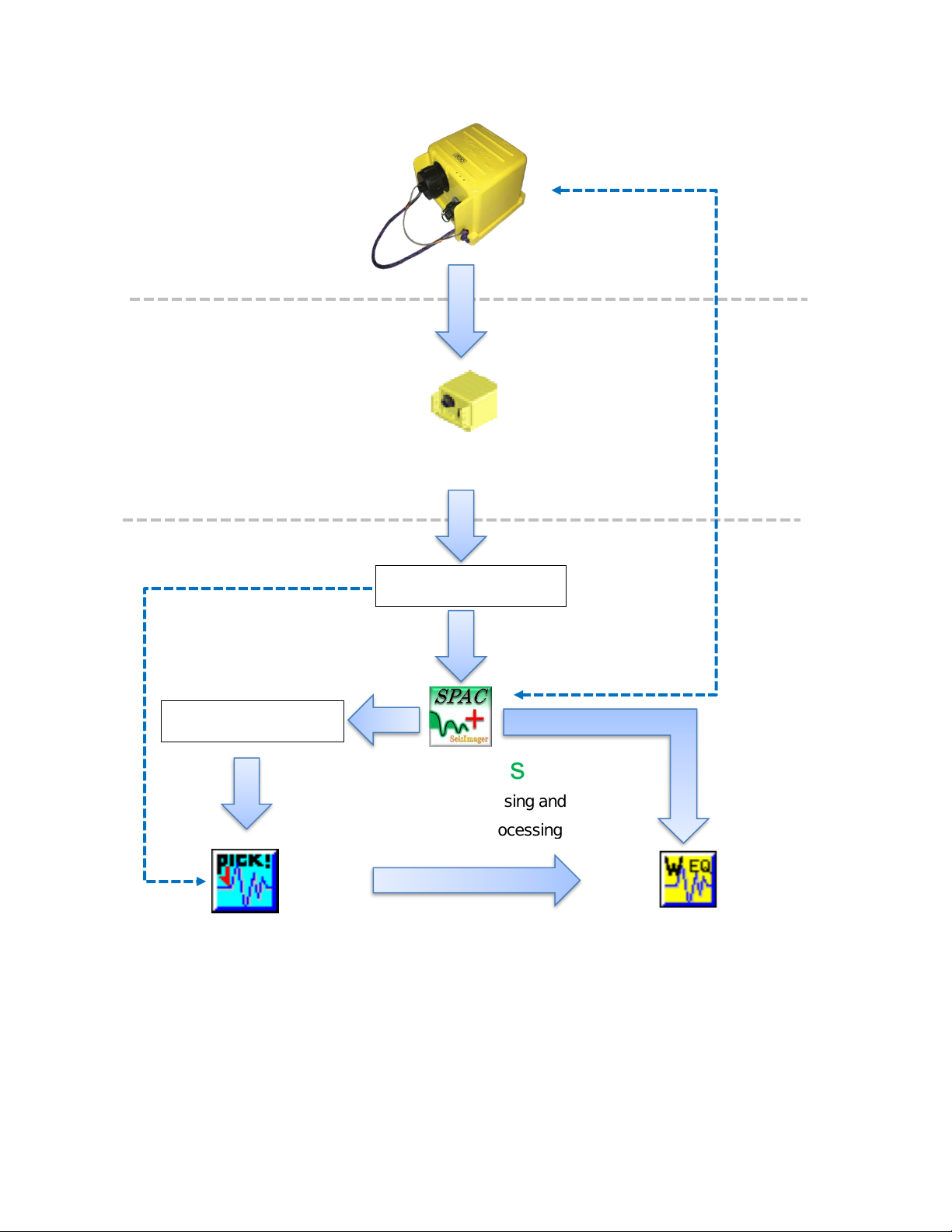
Figure 1.1 summarizes software suite and modules will be mentioned in this manual and outline of data

processing. Two software suites, Geometrics Atom Downloader and SeisImager will be used to download

waveform data from Atom and to process the data. Geometrics Atom Downloader downloads waveform data

from Atom AUs via Wi-Fi and save it raw data files (.mtn). SPACPlus reads the raw data, edits and pre-process

raw data and save it as SEG2 files. It also calculates an 1D dispersion curve from ambient noise data. Pickwin

takes over pre-processed data and applies 2D or 3D dispersion curves. Pickwin also directory reads the raw

data file (.mtn). WaveEq applies various inversions to 1D to 3D dispersion curves and provides 1D to 3D S-

wave velocity model. The SPACPlus also downloads data from Atom AUs and set up acquisition parameters

via Wi-Fi or USB.

Although the manual mainly describes data acquisition and processing for 1D passive and active surface wave

methods, Atom can be used for other seismic surveys such as refraction and reflection. SPACPlus cuts out

and saves shot records as SEG2 files and Pickwin and Plotrefa take over these data and applies refraction or

general seismic processing.

2

02/06/2019, Rev. 1.6

Atom

Geometrics

Atom Downloader

Geometrics

Atom Downloader

Figure 1.1 Software suite and modules described in the manual and outline of processing.

SPACPlus

Pickwin

WaveEq

Raw data file

Data file (.sg2)

2D/3D surface wave processing

Editing, pre-processing and

1D surface wave processing

Dispersion curve analysis

Download data via Wi-Fi.

Download data via Wi-Fi or USB.

3

02/06/2019, Rev. 1.6

2. Typical survey configuration for microtremor array measurements (MAM)

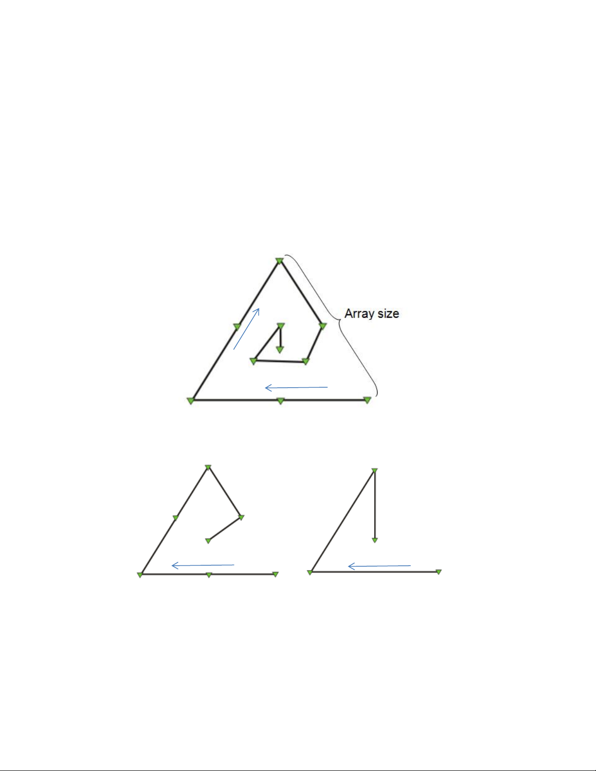
1) In microtremor array measurements (MAM), the array size (or maximum separation of receivers) must be

larger than the depth of investigation. For example, the array size must be bigger than approximately 30 m in

the investigation for an AVS30 investigation. SeisImager allows four set types of array configurations as well

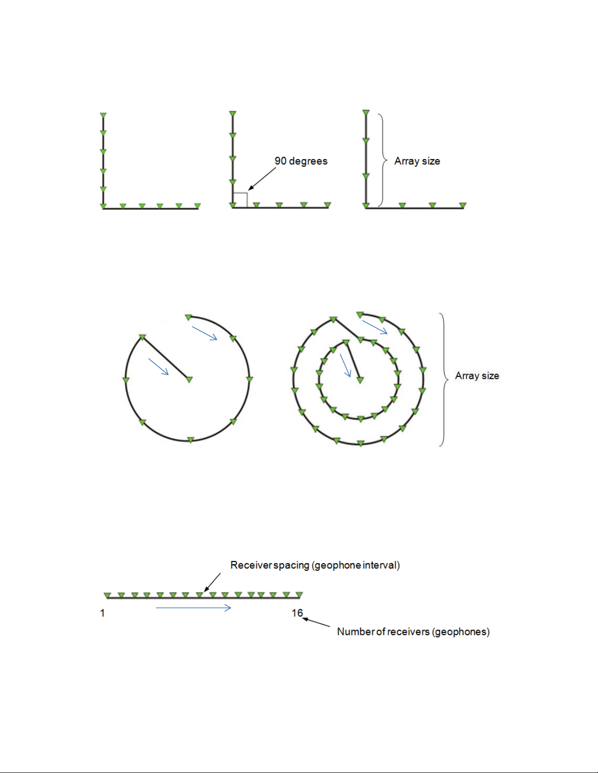
as a custom option. Figures 2.1 through 2.5 illustrate the various set configurations. Note that “Array size” in

the Figures is the definition used for processing in SeisImager and not the same as the maximum receiver

separation. See SeisImager/SW manual for more details. As in Figure 1, the black line represents the order

of the Atom’s ID and the green inverted triangles represent each Atom.

Start

End

Figure 2.2 Map view of MAM survey equilateral triangle spread configurations with 7 (Triangle 7)

and 4 geophones (Triangle 4).

Figure 2.1 Map view of MAM survey equilateral triangle spread configuration with 10 geophones

(Triangle 10).

Start

End

Start

End

4

02/06/2019, Rev. 1.6

Start

Figure 2.4 Map view of MAM survey circle spread configurations with 8 outer geophones on one circle

and one center geophone (Single circle 9) and 18 geophones in two circles and one center geophone

(Double circle 37).

Start

End

End

Figure 2.5 MAM survey linear spread configuration using all channels, one per geophone.

Start

End

Figure 2.3 Map view of MAM survey L-shape spread configurations with 11 (L11), 9 (L9), and 7
(L7) geophones. An angle between two edges does not need to be 90 degrees.

End

Start

Start

End

Start

End

5

02/06/2019, Rev. 1.6

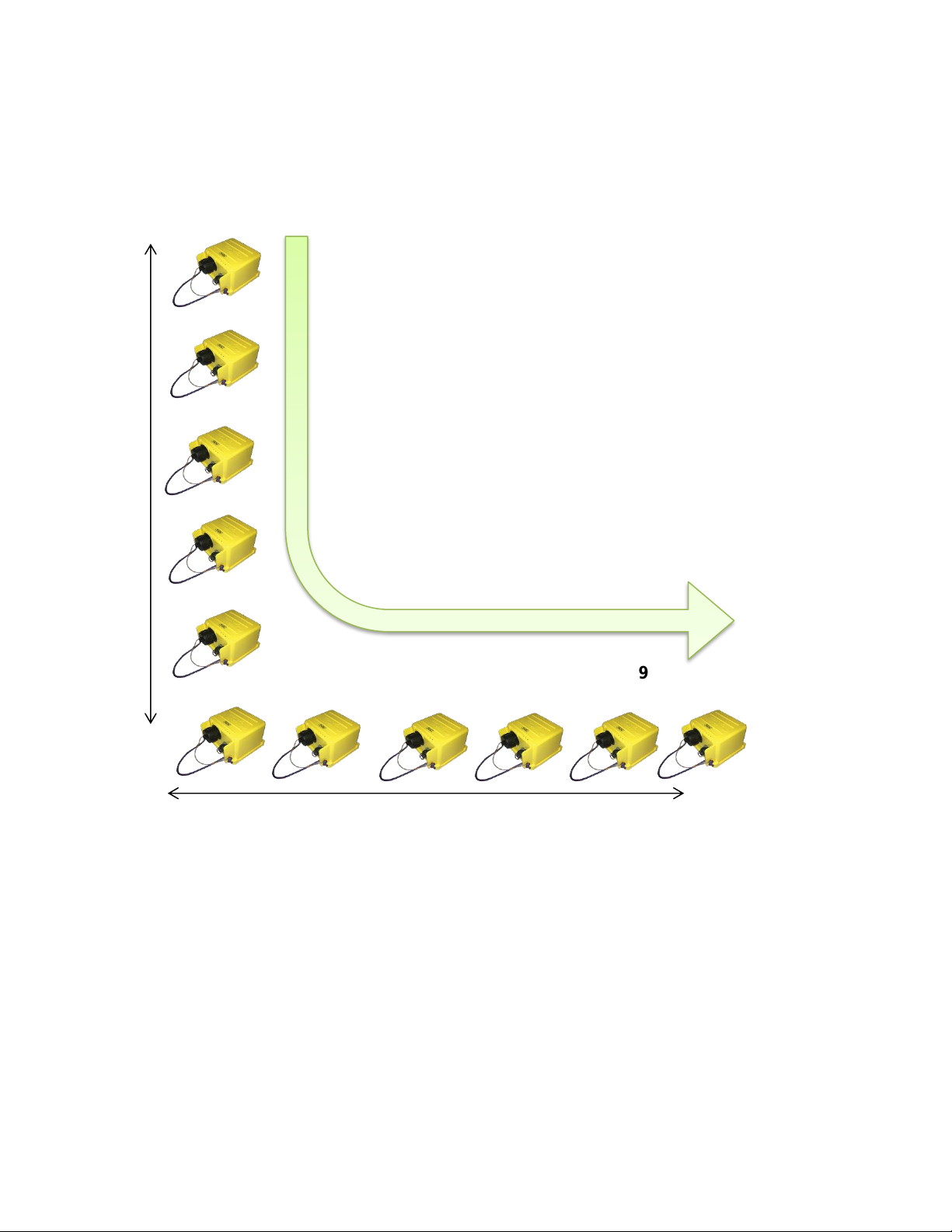
2) A typical example of an L-shape array for an AVS30 survey using Atom units is shown below. For the sake

of simplicity, deploy the Atoms in numerical order of ID. In this example, the Atom ID’s are 10006 to 100050.

25 ~ 75 m

25 ~ 75 m

100011

100006

100014

100015

100027
100031

100036

100038

100039

100049

100050

Deploy Atom units in numerical order

Figure 2.6 L-shaped array (L11) using 11 Atom AUs.

6

02/06/2019, Rev. 1.6

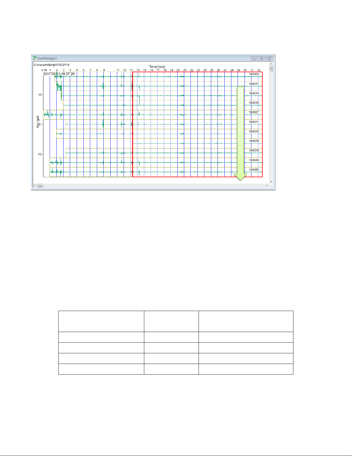
During processing, waveform traces are shown and processed in the numerical order of each Atom unit’s ID.

3) Data acquisition

For an S-wave velocity investigation, such as an AVS30, record between 15 to 30 minutes of ambient noise

per survey. This will be sufficient for surveys with penetration depth of 30 to 100 meters. As arrays become

larger, increase the recording time. Standard recording time for different size arrays is summarized in Table

2.1. Note that the standard time is just a rough indication and is dependent on site conditions. For surveys

larger than 100 meters in urban areas, it is better to acquire the data at night.

Table 2.1 Array size and standard recording time

Array size or investigation

depth (m)

Recording time

(min.)

Remark
< 30

> 15

NA

30 ~ 100

> 30

NA

100 ~ 500

> 45

In urban areas, survey at night

500 <

> 60

In urban areas, survey at night

Traces are shown and

processed in numerical order

Figure 2.7 Example of data obtained from Atom units.

7

02/06/2019, Rev. 1.6

3. Typical survey configuration for multi-channel analysis of surface waves (MASW)

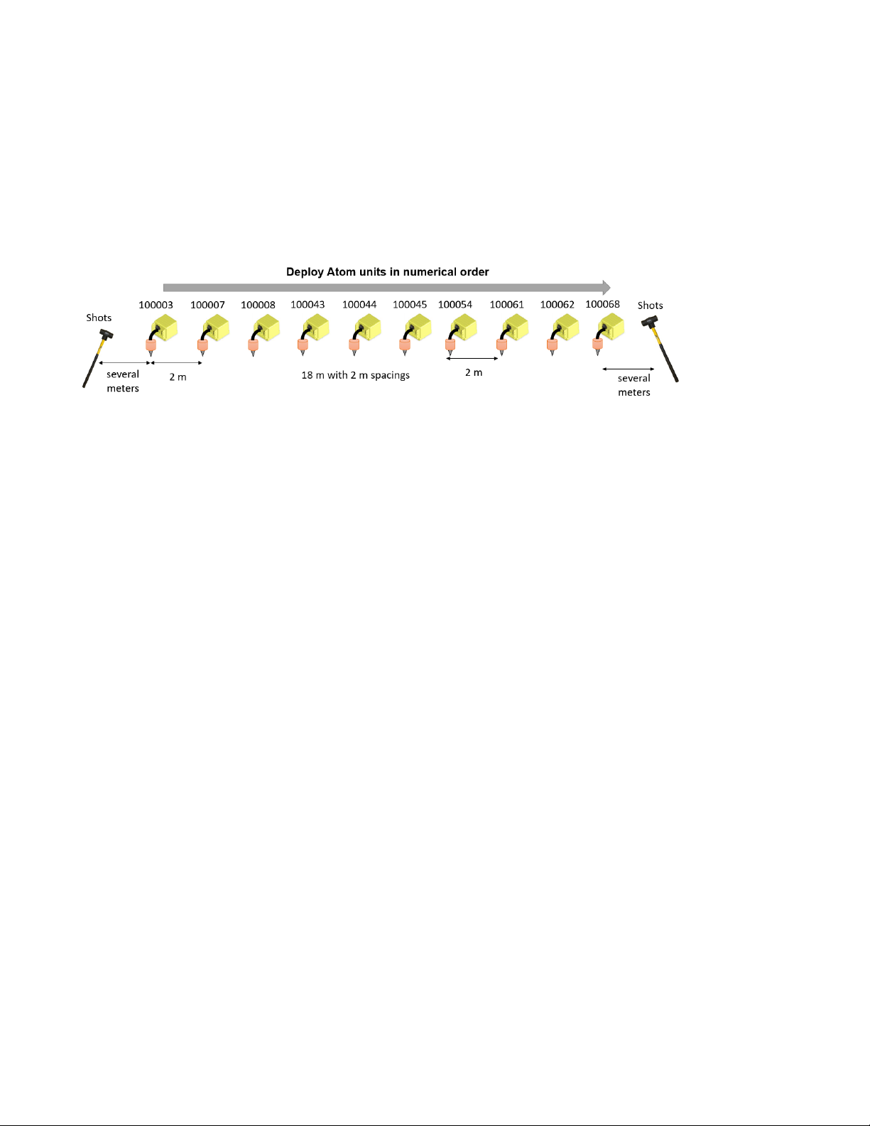
In multi-channel analysis of surface waves (MASW), the array size (spread length or maximum separation of

receivers) must be larger than the double of investigation depth. For example, the array size must be bigger

than approximately 20 m in the investigation depth of 10 m. Figures 3.1 illustrates the typical configurations.

Figure 3.1 Typical source-receiver geometry for multi-channel analysis of surface waves

(MASW).

8

02/06/2019, Rev. 1.6

4. General operation of Atom

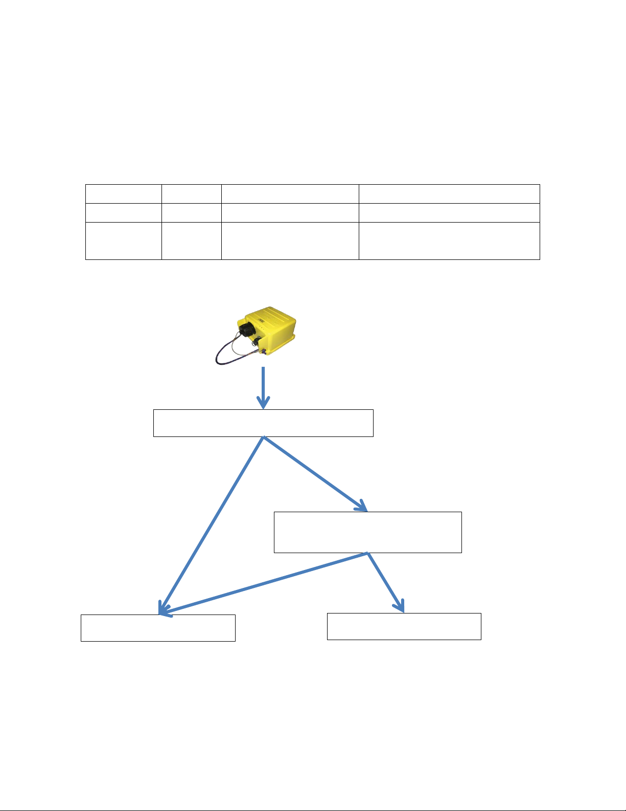
The atom generally has two modes of operation. The first is the recording mode without Wi-Fi and the second

mode is downloading with Wi-Fi.

Table 4.1 Recording mode and downloading mode

Mode

Wi-Fi

Wi-Fi LED

Operation

Recording

Off

No blinking or blink once

Recording data

Downloading

On

Blink twice

Downloading data

Set up acquisition parameters

Figure 4.1 describes the behavior of Atom when turned on.

Figure 4.1 Recording mode and downloading mode for Atom

Found an access point “atom0000”?

Received search command from

“Geometrics Atom Downloader”?

Downloading mode

Recording mode

Turn on

No

Yes

No

Yes

9

02/06/2019, Rev. 1.6

Operations for the Atom’s two modes can be summarized as follows:

A) Recording mode
1 : Turn off Atom.
2 : Turn off access point “atom0000”.
3 : Turn on Atom.

B) Downloading mode
1 : Turn off Atom.
2 : Turn on access point “atom0000”.
3 : Connect PC to the access point “atom0000” by LAN cable (recommended) or Wi-Fi.

4 : Launch Geometrics Atom Downloader .
5 : Turn on Atom.

5. LED Colors on Atom

Battery Wi-Fi

GPS

Figure 5.1 Color LEDs of Atoms.

10

02/06/2019, Rev. 1.6

6. Start and stop recording

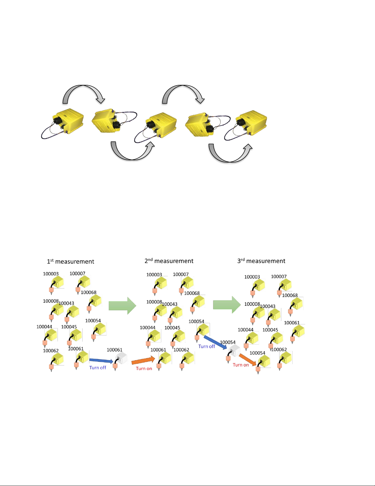
Atom can be turned off via the Wi-Fi connection (8. Confirm or set up the Atom’s acquisition parameters via

Wi-Fi). To distinguish measurements, turn off and on one unit at the beginning or ending of the measurements.

Figure 6.2 Turning on and off of Atom units between measurements.

To begin recording, turn each unit over slowly two or three

times.

Unit Beeps when the Atom is turned on or off.

Figure 6.1 Turning on and off of Atom units.

11

02/06/2019, Rev. 1.6

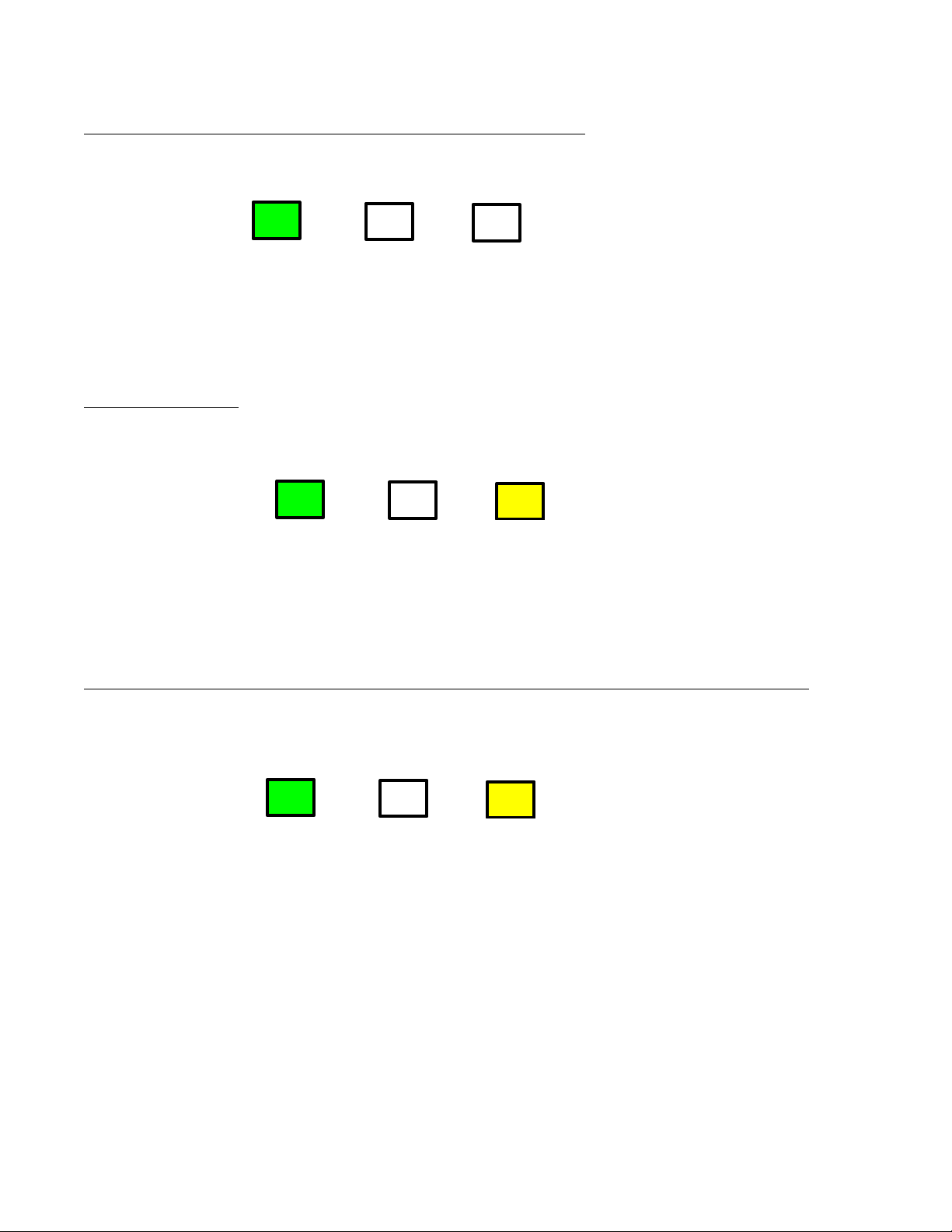
When power is turned on, the LED indicator lights show the following:

When GPS is locked:

After recording begins: (recording automatically starts several tens of seconds after GPS is locked).

Battery Wi-Fi

GPS

Slow blink

Slow blink

Figure 6.4 LEDs when Atom is locked on the GPS.

Battery Wi-Fi

GPS

Slow blink

Fast blink

Figure 6.5 LEDs when Atom is recording data.

Battery Wi-Fi

GPS

Figure 6.3 LEDs when Atom is turned on.

12

02/06/2019, Rev. 1.6

7. Battery status

The battery lasts approximately 60 to 70 hours from a full charge.
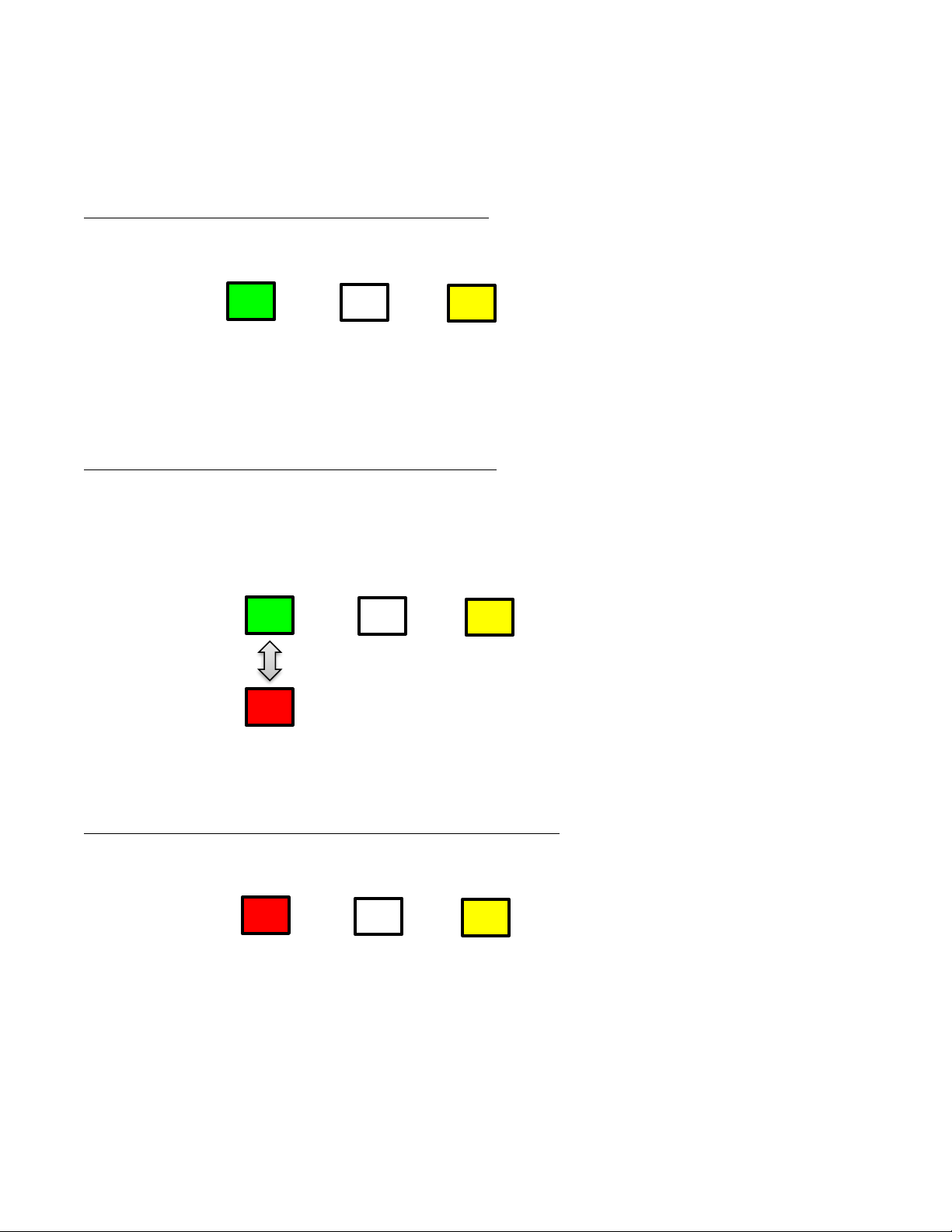
Battery status when data is being recorded (full battery).

Battery status when data is being recorded (less battery).

As the battery charge decreases, the green and red lights alternate. It usually takes more than 40 hours of

use after a full charge for the red LED to start blinking.

Battery status when data is being recorded with a very low battery

Battery Wi-Fi

GPS

Slow blink
Fast blink

Figure 7.1 LEDs while data is being recorded (full

battery).

Battery Wi-Fi

GPS

Increase in blinking red LED corresponds to

decreasing battery charge.

Quick blink

Figure 7.2 LEDs while data is being recorded

Battery Wi-Fi

GPS

Slow blink

Quick blink

Figure 7.3 LEDs when data is being recorded with a very

low battery

13

02/06/2019, Rev. 1.6

8. Confirm or set up the Atom’s acquisition parameters via Wi-Fi

Use Geometrics Atom Downloader confirm or set up Atom’s Acquisition parameters. The parameters can be

also confirmed or set up using SPACPlus via Wi-Fi or USB. See appendix A and C for the more details about

SPACPlus.

1) Turn off and stop recording for all Atom units.

2) Plug in a Wi-Fi access point to your PC.

3) Connect your PC to “atom0000” by LAN cable (recommended) or Wi-Fi. Do not connect both LAN cable

and Wi-Fi to the access point.

4) Launch Geometrics Atom Downloader .

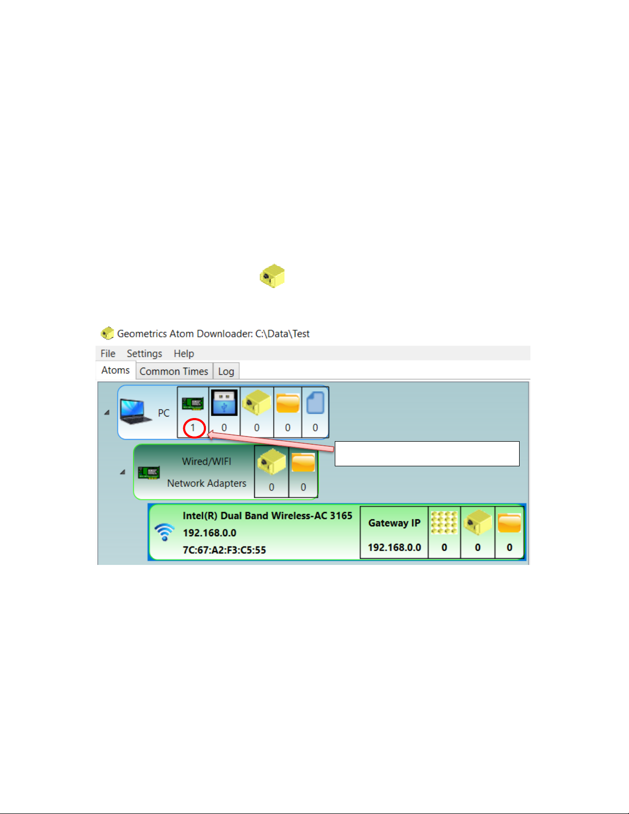
5) Display shown below appears on the window. Make sure one or two networks were found.

Number of networks should be 1

Figure 8.1 Display of Geometrics Atom Downloader

when no Atom was found.

14

02/06/2019, Rev. 1.6

6) Turn on all Atom units.

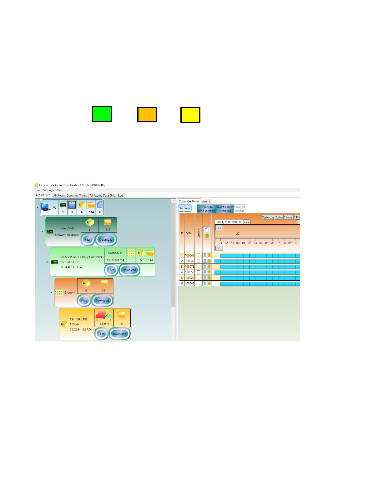
The Atom units automatically being download mode (Figure 8.2) when they locate the access point “atom0000”.

In this mode, data recording does not start.

The Geometrics Atom Downloader shows the number of Atom AUs found.

Battery

Wi-Fi

GPS

Slow Blink.

Slow blink when GPS is locked.

Blink twice.

Figure 8.2 LEDs when Atom is ready to be controlled from

Figure 8.3 Display of the Geometrics Atom Downloader

when 6 Atom AUs were found.

15

02/06/2019, Rev. 1.6

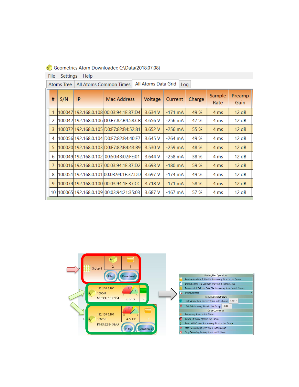
7) Click [All Atoms Data Grid] tab on the left side window of the Dowanloader, you will see each Atom units’

ID, IP address, battery voltage, sampling time and pre-amp gain. Note that the default setting of passive

surface wave methods is 4.00 ms and 12.0 db,

8) To change the Atom unit’s acquisition parameters, click a right button of a mouse in group (to change all

AUs in group) or in each Atom (to change indivdual AU) to show sub menus.

Figure 8.4 Example of Atoms Data Grid showing the acquisition parameters

and conditions of each Atom AU.

Figure 8.5 Click group or individual Atom to change acquisition parameters.

Group

Each AU

Click a right button of a mouse to

show sub menus

16

02/06/2019, Rev. 1.6

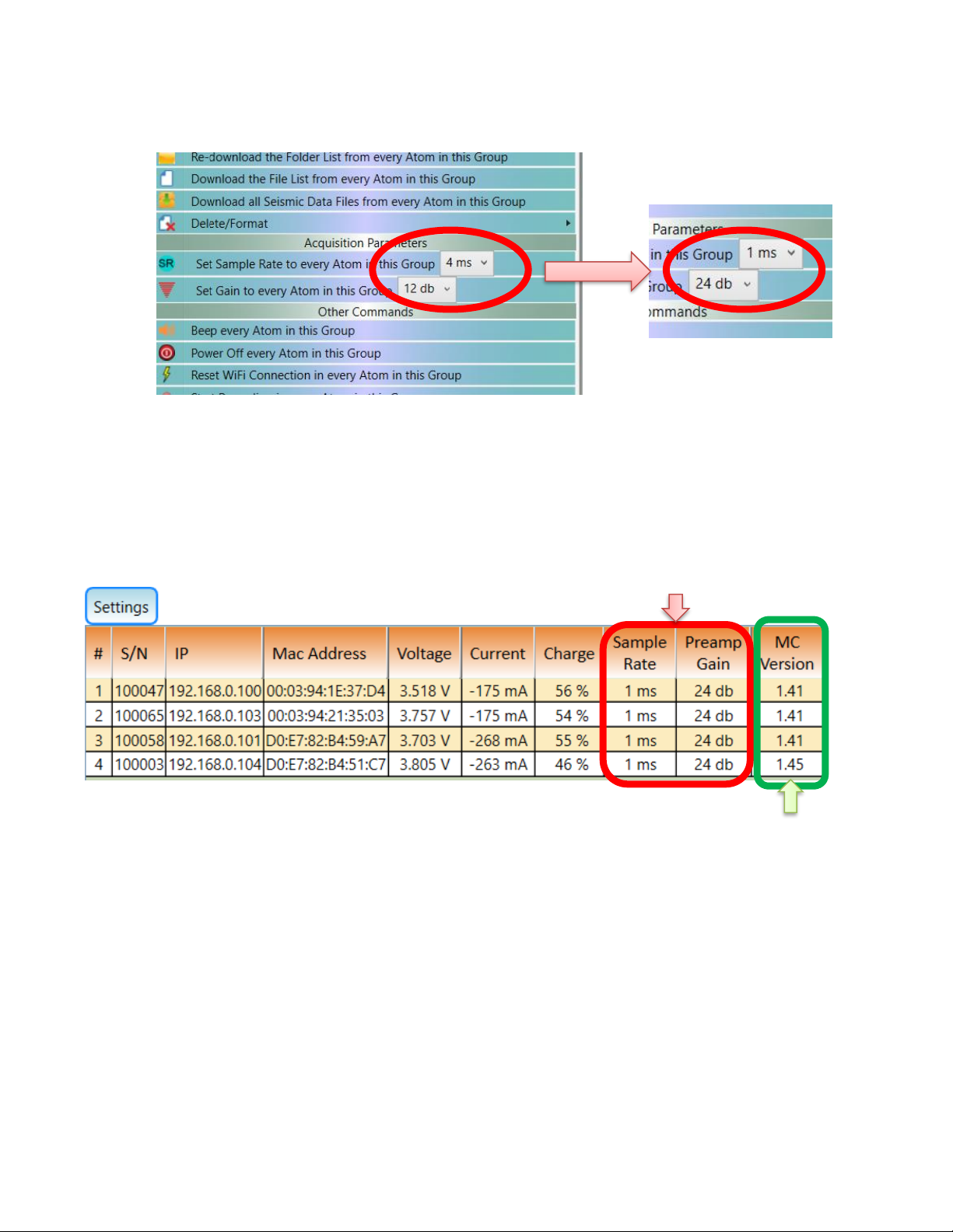
9) Select sampling time and preamp gain in a dialog box.

10) Confirm changes to the acquisition parameters, in the Atom Data Grid.

Note that if the MC version is smaller than 1.39, acquisition parameter may not be changed by Atom

Downloader. Use SPACPlus to change the acquisition parameter if the Atom Downloader did not work. See

Appendix A for the details.

Figure 8.6 Change sampling time and/or preamp gain.

Figure 8.7 Acquisition parameters shown in Atoms Data Grid.

Acquisition parameters

MC version

17

02/06/2019, Rev. 1.6

9. Use Wi-Fi to turn off all Atom units

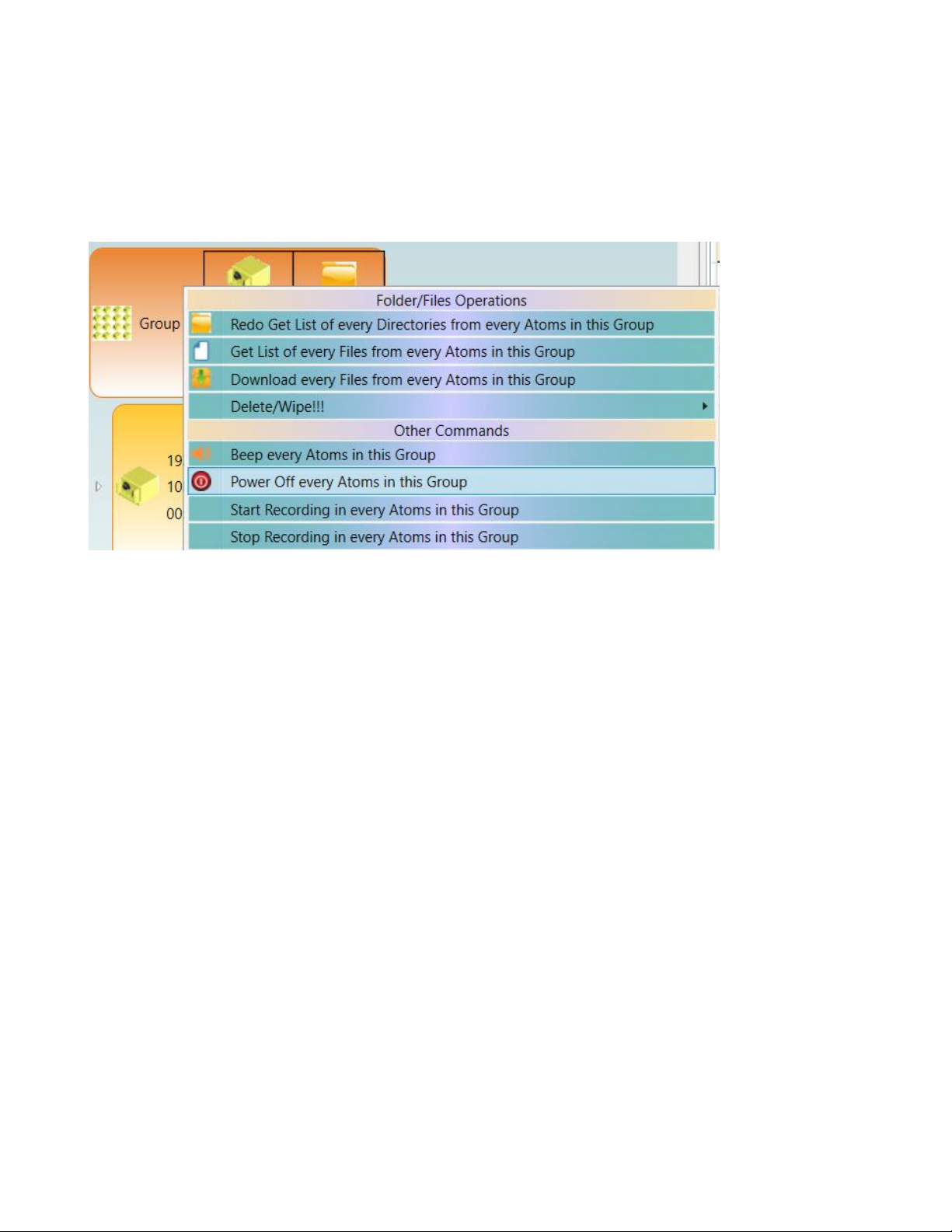
1) To turn off all Atom units, show a sub menu by clicking a right button of a mouse either on group or on

each AU. Select [Power off every Atoms in the Group] of [Power off this Atom] to turn off Atom units.

2) Confirm all boxes were turned off.

Figure 9.1 Sub menu to turn off Atom units.

18

02/06/2019, Rev. 1.6

10. Battery charging

Charging begins when the Atom is connected via charging cable to the USB connector.
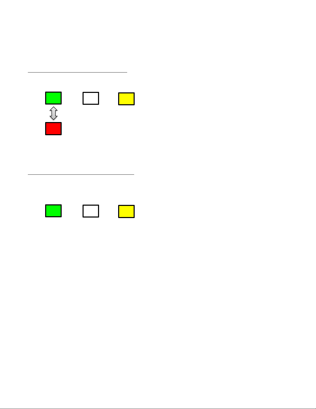
Battery charging status (during charging).

Battery charging status (charging complete).
Charging takes approximately 10 hours from fully discharged battery.

Battery Wi-Fi

GPS

The green light blinks get as charging proceeds.

Slow blink when GPS is locked.

Figure 10.1 LEDs when Atom is being charged.

Battery Wi-Fi

GPS

Steady on.

Blink slowly when GPS is locked.

Figure 10.2 LEDs when battery fully charged.

19

02/06/2019, Rev. 1.6

11. Data format

The format of waveform data file is the almost same as MT-Neo. The extension is “.atm” instead of “.mtn”.

The files can be opened by Pickwin.

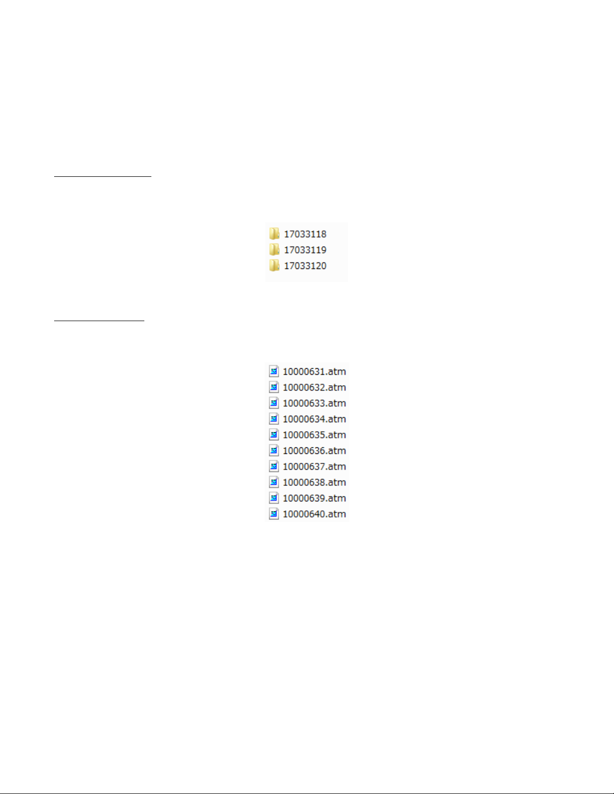
Folder for each hour.

The data files are automatically saved to the date and time (UTC) the data is collected. In the example shown

below, the folders represent data collect on March 31

st

, 2017 between 18:00 and 20:00 UTC.

Waveform data file.

Collected data are stored in files named for the Atom unit’s ID and time in minutes. In the example shown

below, files are recorded with Atom unit 100006 from 31 to 40 min.

20

02/06/2019, Rev. 1.6

12. Data download

There are three methods for retrieving data from the Atom.

A) Copy data from SD card

Remove the SD card from each Atom box and directly copy waveform files. Data files are saved in folders as

shown above.

B) USB

Connect the USB cable from your PC to your Atom and download waveform data files in SPACPlus using the

following menu commands: [File]>>[ATOM(USB)]>>[Download via USB]. Set Baud rate to 3686400.

Download the USB driver from a link shown below and install it at first time.

http://seisimager.esy.es/atom/utility/CDM_2_08_30.zip

See Appendix B for the details.

C) Wi-Fi

Geometrics Atom Downloader downloads waveform data files via Wi-Fi using a special access point

connected to your PC. Wireless downloading is faster than downloading via USB connection with data

downloading from several Atom units simultaneously. SPACPlus also downloads waveform data via Wi-Fi if

the Atom Downloader is not available (see Appendix A for the details). Follow the procedure shown below to

download waveform data using the Geometrics Atom Downloader.

1) Turn off each Atom to stop recording data.

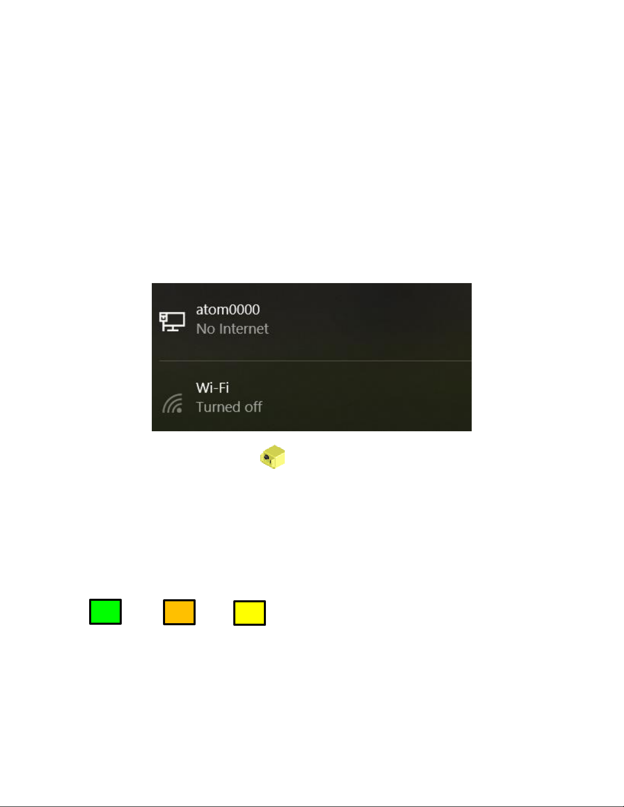
2) Plug in a Wi-Fi access point (SSID of “atom0000”) to your PC.

3) Connect your PC to “atom0000” by LAN cable (strongly recommended) or Wi-FI. Do not connect both Lan

cable and Wi-Fi to the access point. It is better to turn off Wi-Fi to make sure only the Lan-cable is connected

to the access point.

21

02/06/2019, Rev. 1.6

4) Launch Geometrics Atom Downloader .

5) Select [Settings]>>[Data Folder Location] and select a folder to which data to be downloaded

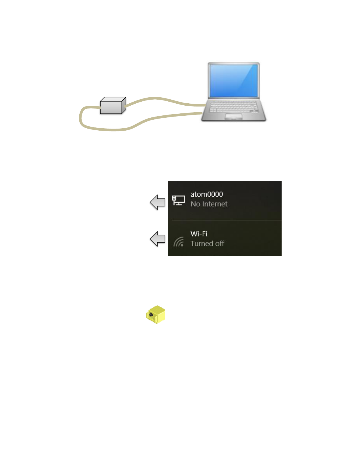
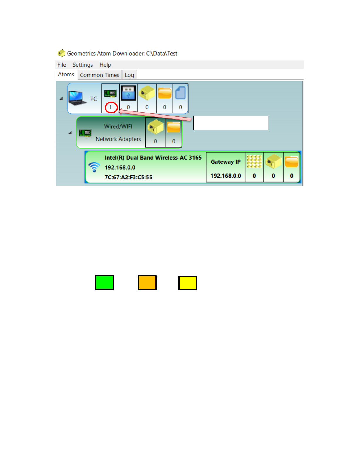
6) Display shown below appears on the window. Make sure one or two networks were found.

Figure 12.1 Connecting access point to PC by Lan-cable.

Power cable (USB)

Lan cable (Ethernet)

Connected to Ethernet by Lan-cable

(should be No Internet).

Wi-Fi is turned off.

22

02/06/2019, Rev. 1.6

7) Turn on all Atom units

The Atom units enter download mode when they find the access point named “atom0000”. In this mode, the

data recording does not start.

Number of networks.

Figure 12.2 Display of Geometrics Atom Downloader

when no Atom was found.

Battery Wi-Fi

GPS

Slow Blink.

Slow blink when GPS

is locked..

Blink twice.

Figure 12.3 LEDs when Atom is ready to download

23

02/06/2019, Rev. 1.6

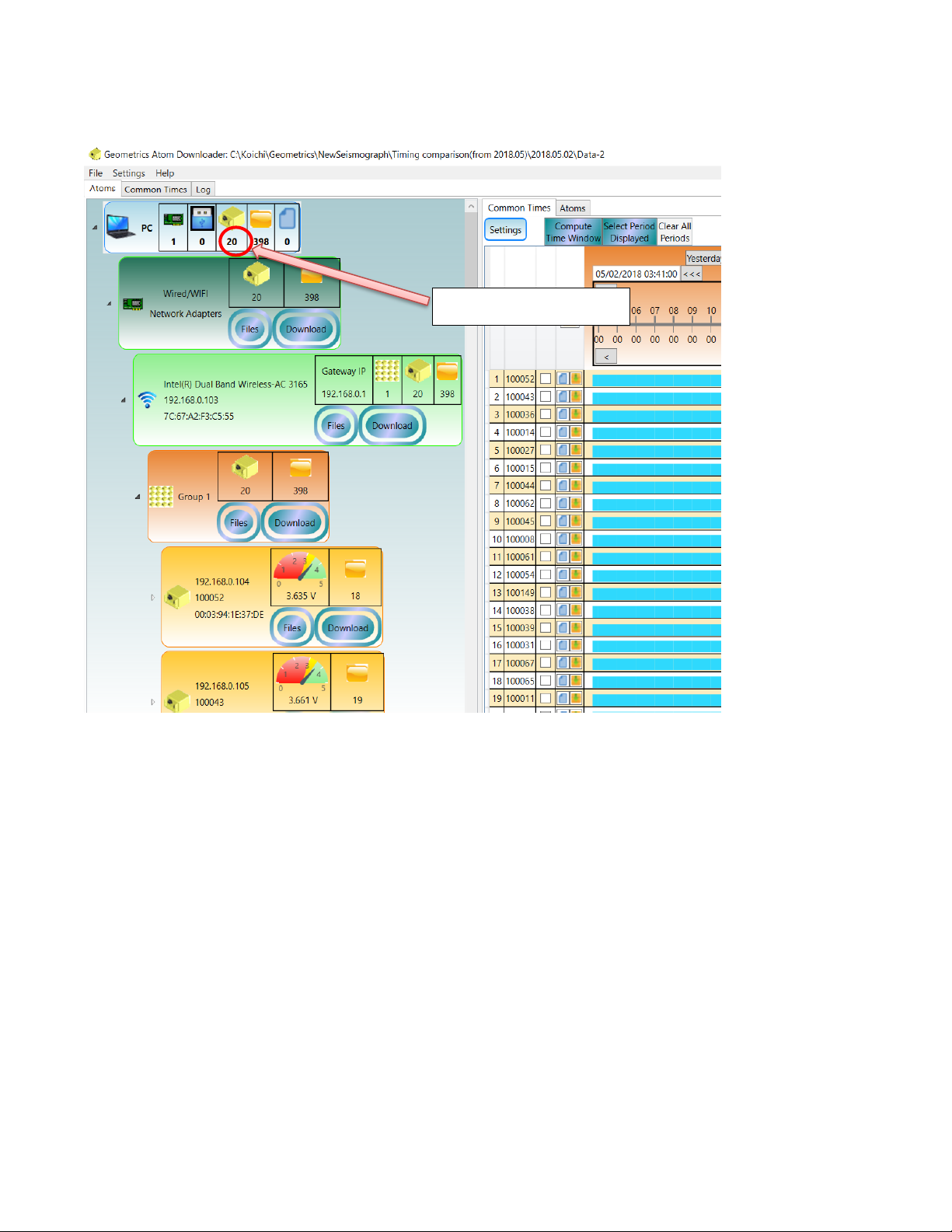
8) Atom IDs appear on the Atom Tree Window of the Downloader.

Number of Atom units.

Figure 12.4 Display of Geometrics Atom Downloader when 20 Atom AUs were found.

24

02/06/2019, Rev. 1.6

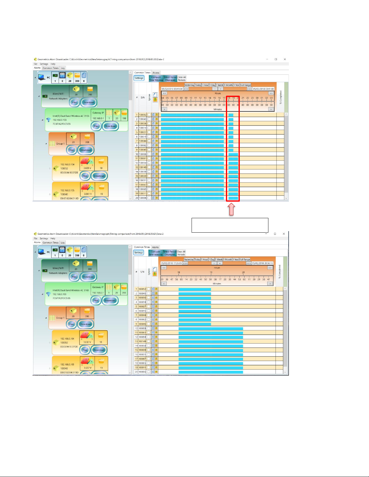
9) Select a time range from which data will be downloaded by a mouse in the windows at right hand side.

10) Click [Compute Time Window] to download common time windows (blocks) or [Select Period Displayed]

to download all data displayed in the window.

Select by a mouse.

Figure 12.5 Selection of data to be downloaded.

25

02/06/2019, Rev. 1.6

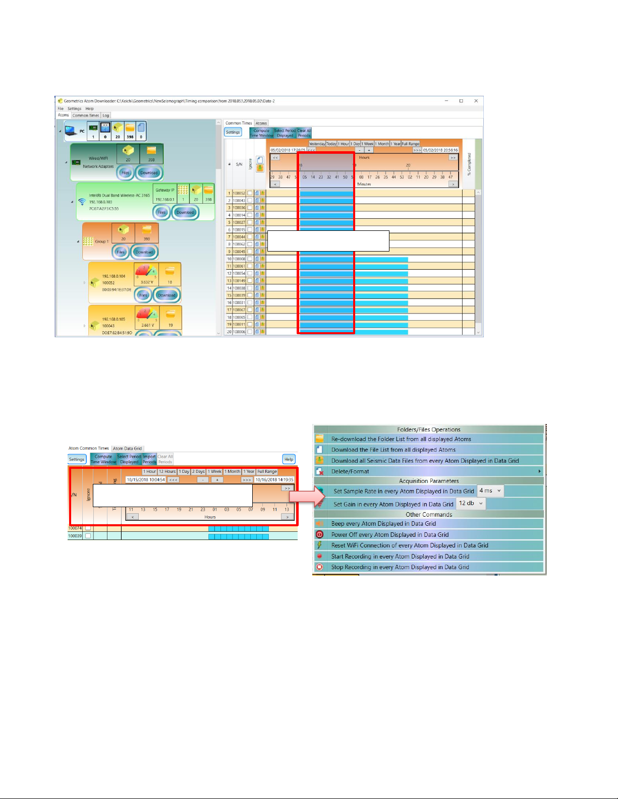
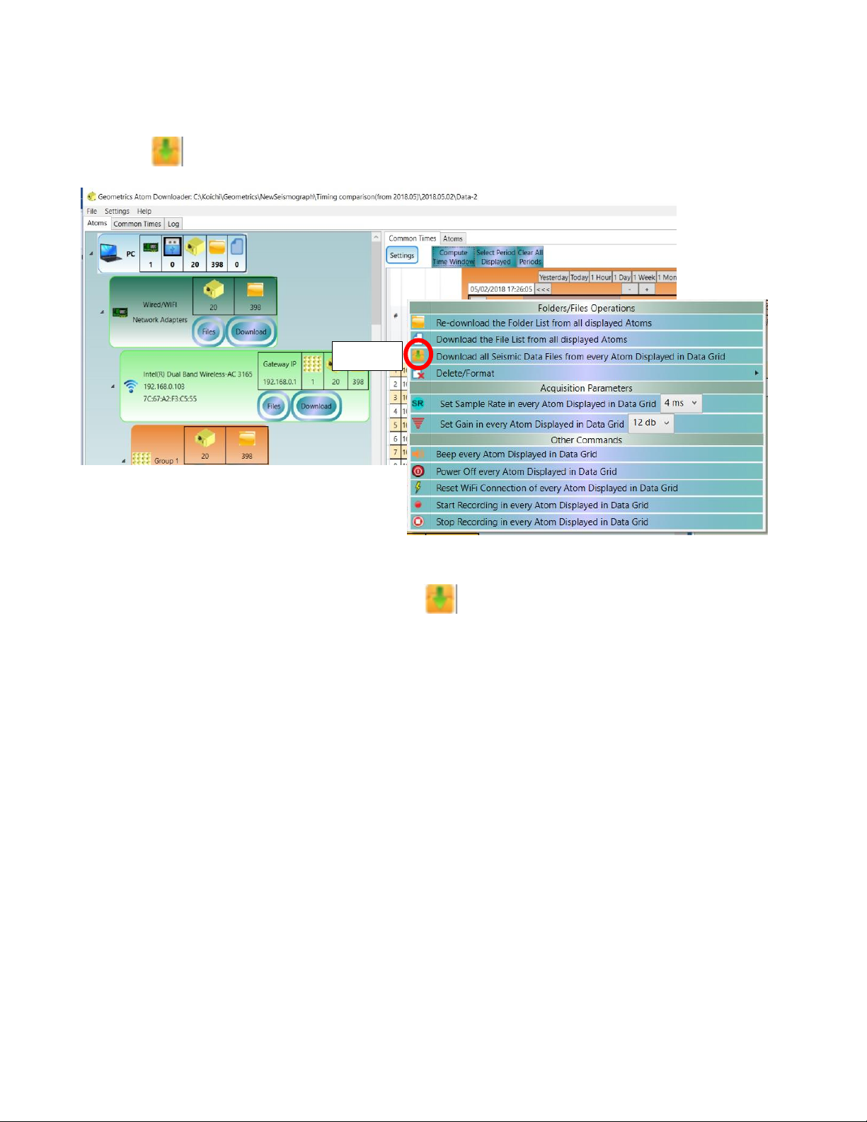
11) Click a right button of mouse in time scale above the Atom data grid to show sub menu.

Figure 12.6 Selection of data to be downloaded.

Figure 12.7 Click a right button of mouse to show sub menu.

Click a right button of mouse

26

02/06/2019, Rev. 1.6

12) Select in the sub menu to start download data.

Figure 12.8 Select to start download data.

27

02/06/2019, Rev. 1.6

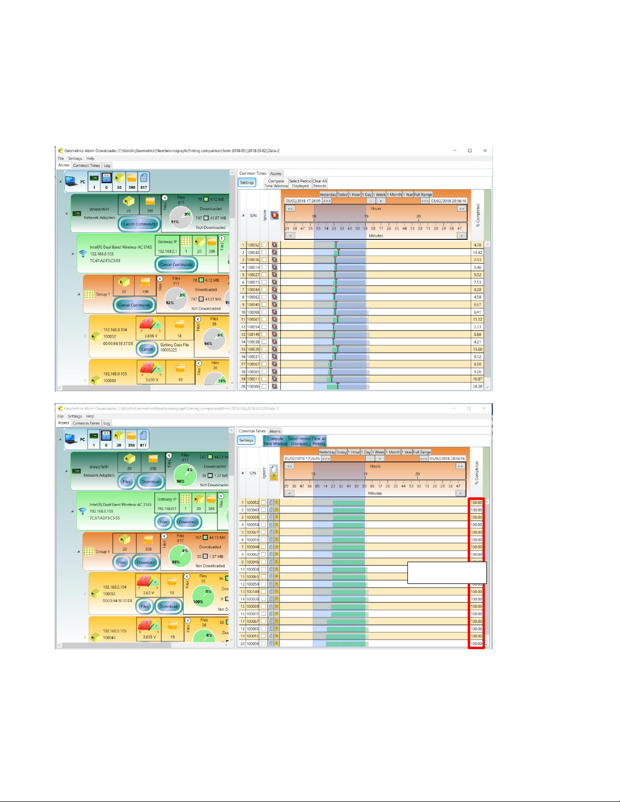
13) During the download process, progress appears on a display similar to the one shown below. After

download completed, completion at the far-right column must be 100 at all rows. Downloaded data has a

folder and file structure shown in 11. Data format.

Figure 12.9 Example of display middle (top) and end of download (bottom).

Must be 100

28

02/06/2019, Rev. 1.6

13. Delete data directory and format SD card

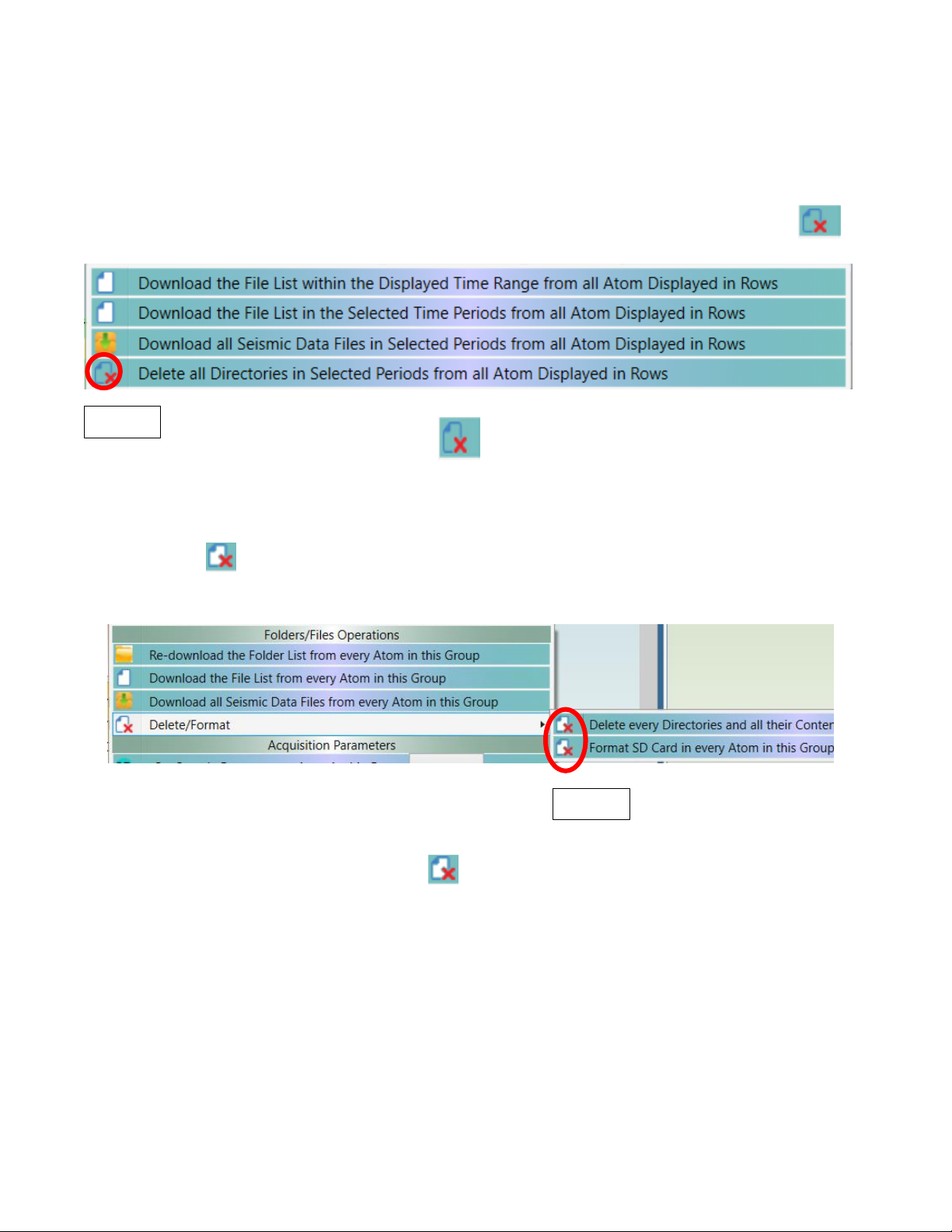
1) Waveform data in Atom AUs can be deleted per directory. To delete directory, select the data in the Atom

Common Times Window (right hand side) just like data download and show sub menus and select .

2) To delete all data in Atom AU or format SD card in the AU, show sub menus in Atom Tree Window (left hand

side) and select .

Figure 13.1 Select to delete data directories.

Figure 13.2 Select to delete data directories.

29

02/06/2019, Rev. 1.6

14. Export waveform data as SEG2 or ASCII file using SPACPlus in SeisImager

Downloaded waveform data can be exported as SEG2 or ASCII file using SPACPlus in SeisImager. Data are

exported with each Common Time Block (CTB) during which all Atom units were recording data. The standard

data exporting procedure is summarized below.

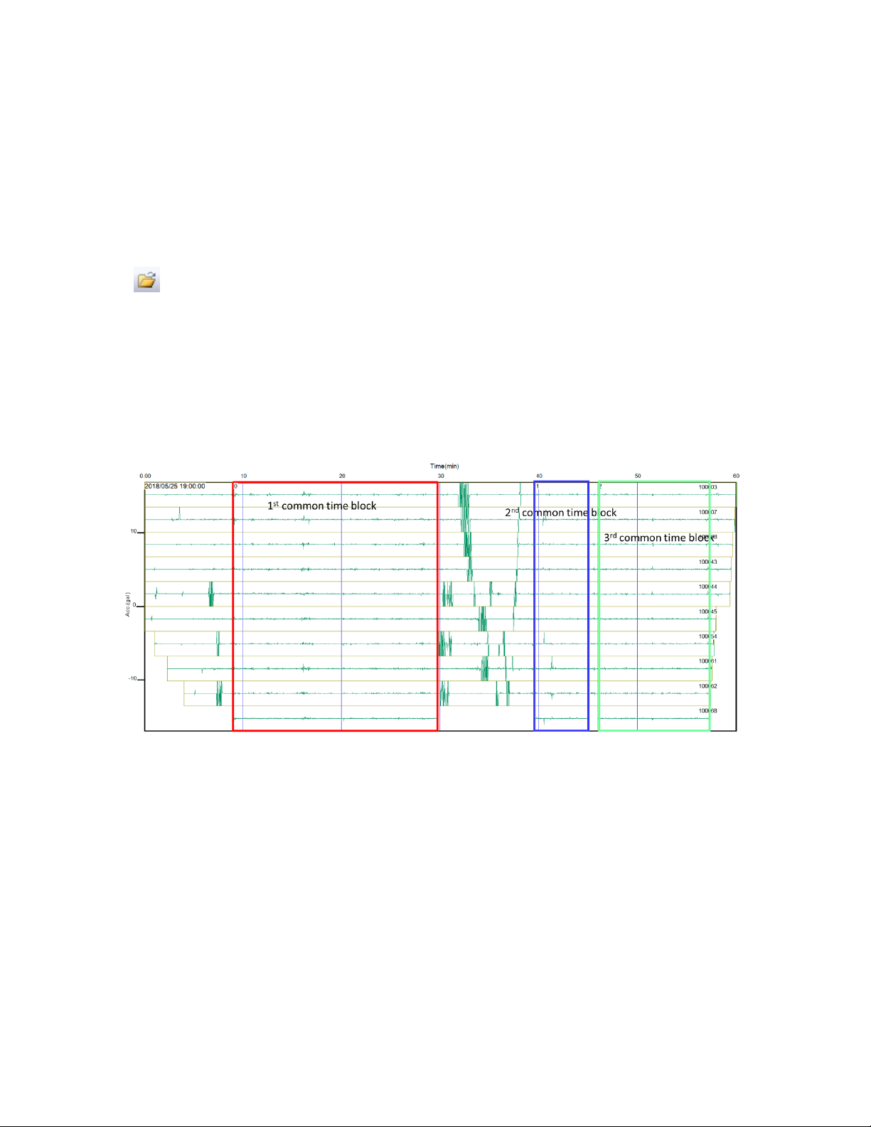
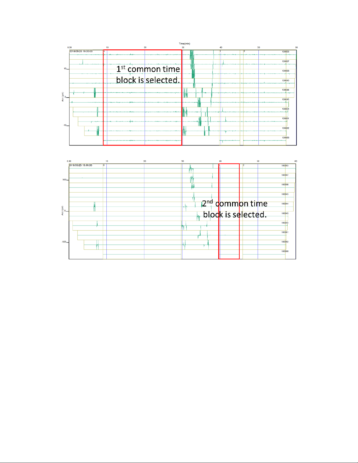
1) Click or select [File]>>[Open folder] to select a folder to which waveform data were downloaded. After

selecting the folder, the waveform data appears as shown below. Waveform traces appear in order from lower

to higher Atom ID numbers. Data processing may be resumed for previously downloaded by selecting

File]>>[Open folder used the last time]. An area surrounded by a red rectangle is a “Common Time Block

(CTB)” during which all Atom units were recording data. Select a CTB to be processed, using left and right

arrows if several CTBs are shown.

Figure 14.1 Selecting the Common Time Block (CTB)..

30

02/06/2019, Rev. 1.6

Figure 14.2 Selecting the Common Time Block (CTB)..

31

02/06/2019, Rev. 1.6

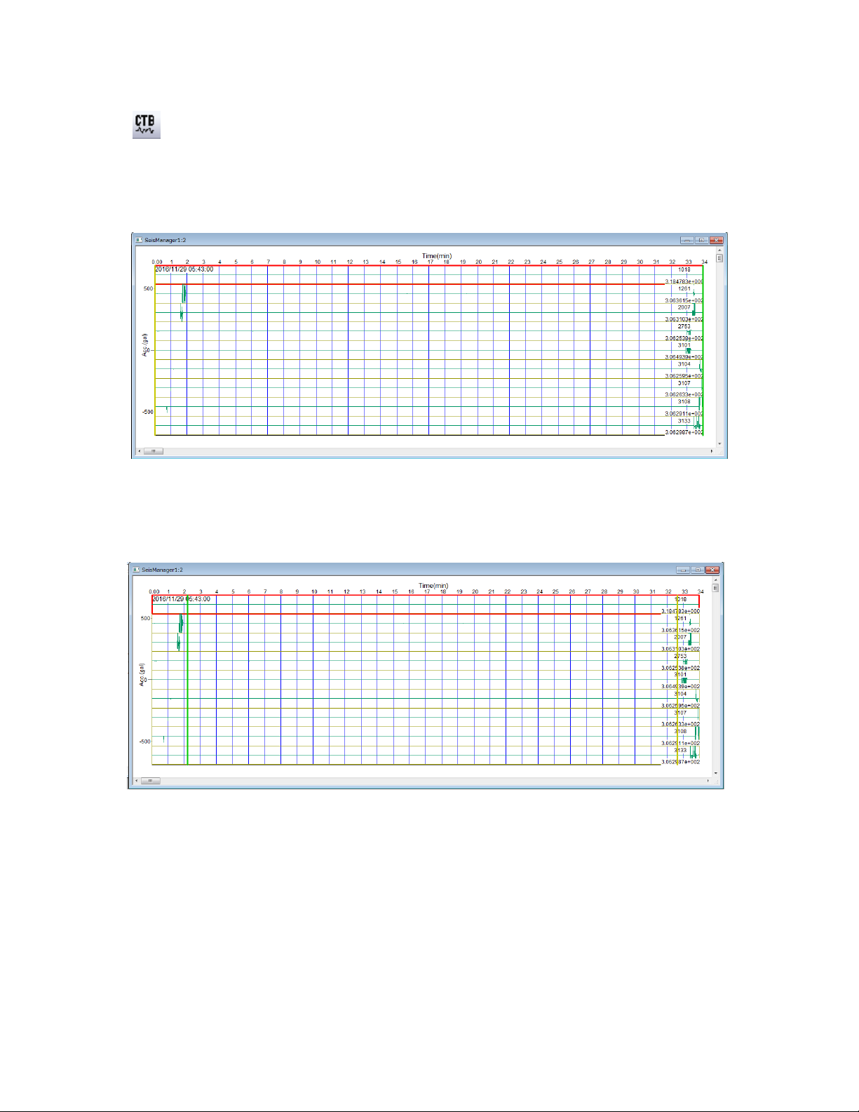
2) Click or select [Window]>>[Processing window] and the selected CTB data (in a red rectangle) will

appear in another window.

3) Optional : Use left and right arrow keys to move gates and the TAB key to switch a gate to be set.

Figure 13.5 Data from the Common Time Block.

Figure 14.3 Window showing the gates (green and yellow lines).

32

02/06/2019, Rev. 1.6

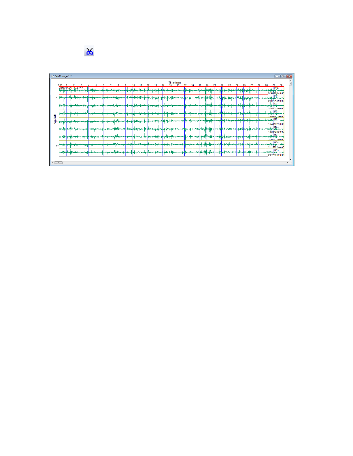
4) Optional : Click or select [Edit]>>[Delete waveform data outside of gate] to delete the waveforms

outside of the gates.

Figure 14.4 Window showing selected data after removing unwanted waveforms.

33

02/06/2019, Rev. 1.6

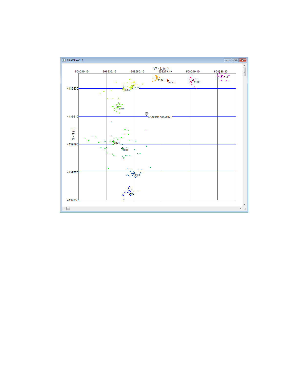
5) Optional : Select [Window]>>[Geometry] to show GPS location as recorded by the Atom units.

6) To save the waveform data in CTB as a SEG2 file, select [File]>>[Save waveform data as SEG2 file].

7) To save the waveform data in CTB as an ASCII file, select [File]>>[Save waveform data as ASCII file].

Figure 13.8 GPS location recorded by Atom units. Small dots indicate GPS locations

recorded by each Atom unit each minute. Medium size circles indicate averaged GPS
location over currently selected time block for each Atom. The large gray circle indicates

averaged location of all Atom units.

34

02/06/2019, Rev. 1.6

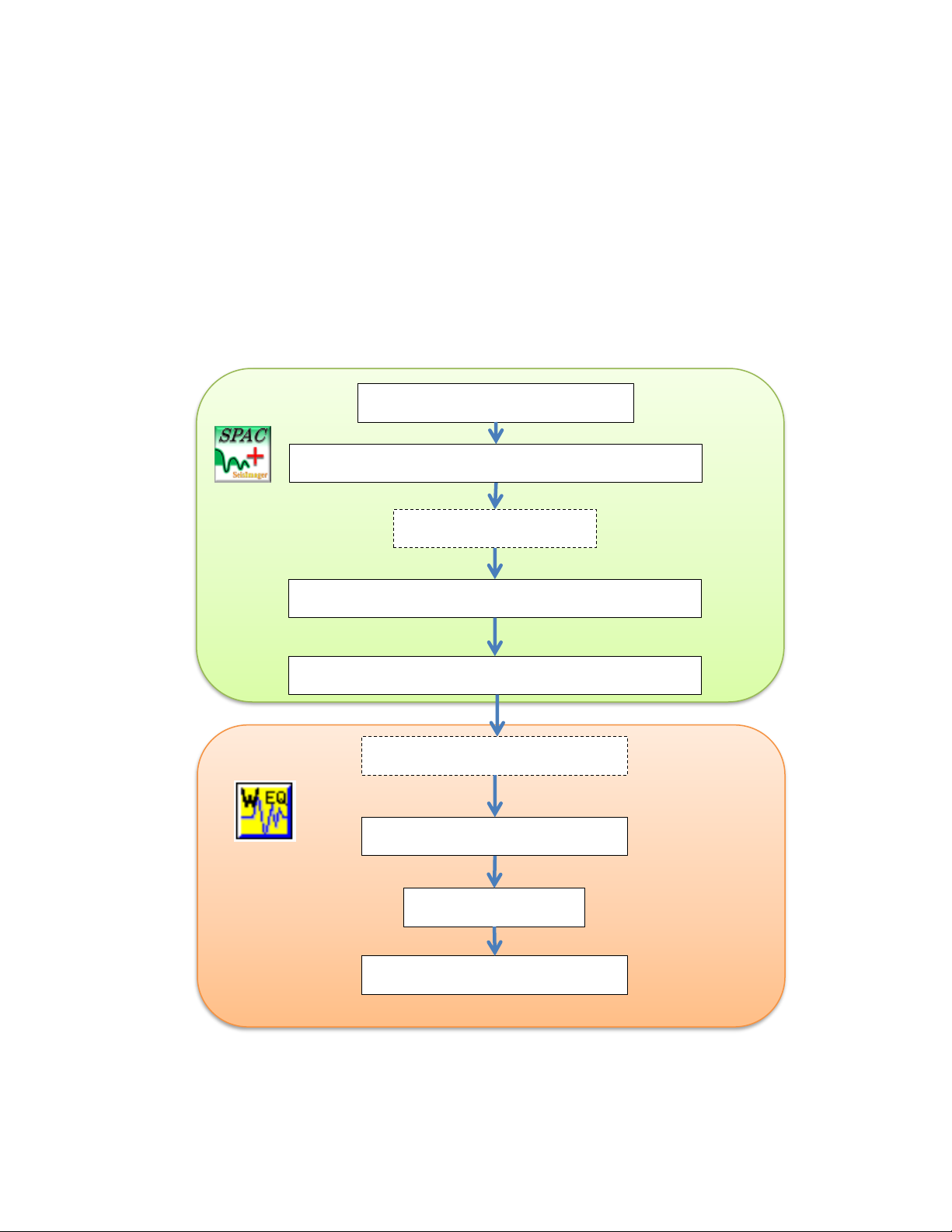
15. Basic passive data processing using SPACPlus in SeisImager.

The basic data processing procedure for 1D passive surface wave method (microtremor array measurements)

is summarized below. Data from an Atom system is processed in the similar way that MASW or MAM surveys

are processed using traditional seismographs such as the Geode. After picking dispersion curves, perform the

data analysis using SeisImager/SW. See “SeisImager/SWTM Manual”, “SeisImager/SWTM Manual Addendum

(H/V)” and “SeisImager/SW-ProTM Manual” for the detailed analysis of dispersion curves and/or H/V curves.

See the section 16 for the data processing procedure for active data recorded by Atom and the section 17 to

combine active and passive data.

Edit dispersion curve (optional)

Create initial curve

Inversion

Final velocity model

WaveEq

Figure 15.1 Basic data processing procedure for microtremor array measurements.

Downloaded data from Atom

Select common time block (CTB) to be processed

Edit CTB (optional)

Calculate spatial auto-correlation

Calculate phase velocity image and pick dispersion

SPACPlus

35

02/06/2019, Rev. 1.6

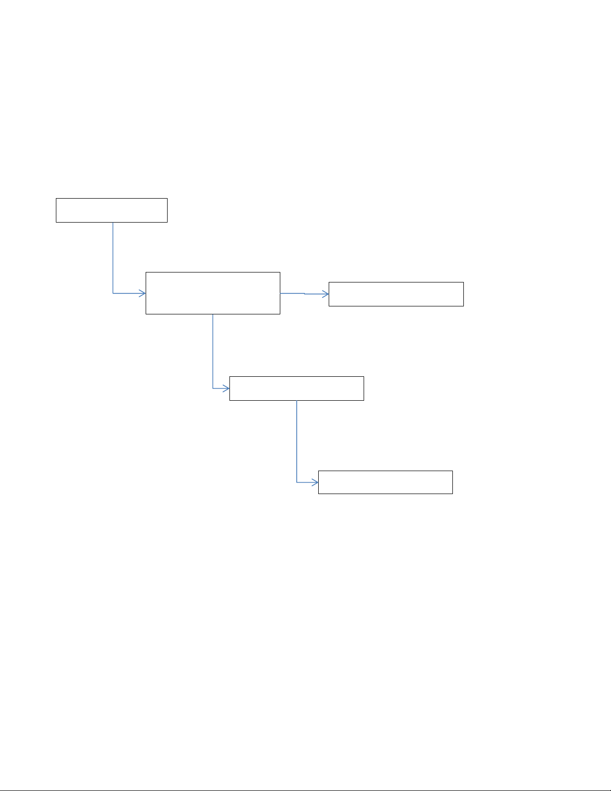
SPACPlus consists of several processing windows which will sequentially appear during processing. Each

window can be viewed one at a time. Several common time blocks (CTB) can be shown in the Main window.

A single CTB can be analyzed at one time. Coherences calculated from several different CTBs can be

appended in the Phase velocity window. Delete other windows (CTB, Geometry, and SPAC) except the Main

window and the Phase velocity window when starting analysis for new CTB,

Main window

Figure 15.2 Windows that appear in SPACPlus.

Common time block

(CTB) window

Geometry window

SPAC window

Phase velocity window

Select one CTB

Set geometry and calculate SPAC

36

02/06/2019, Rev. 1.6

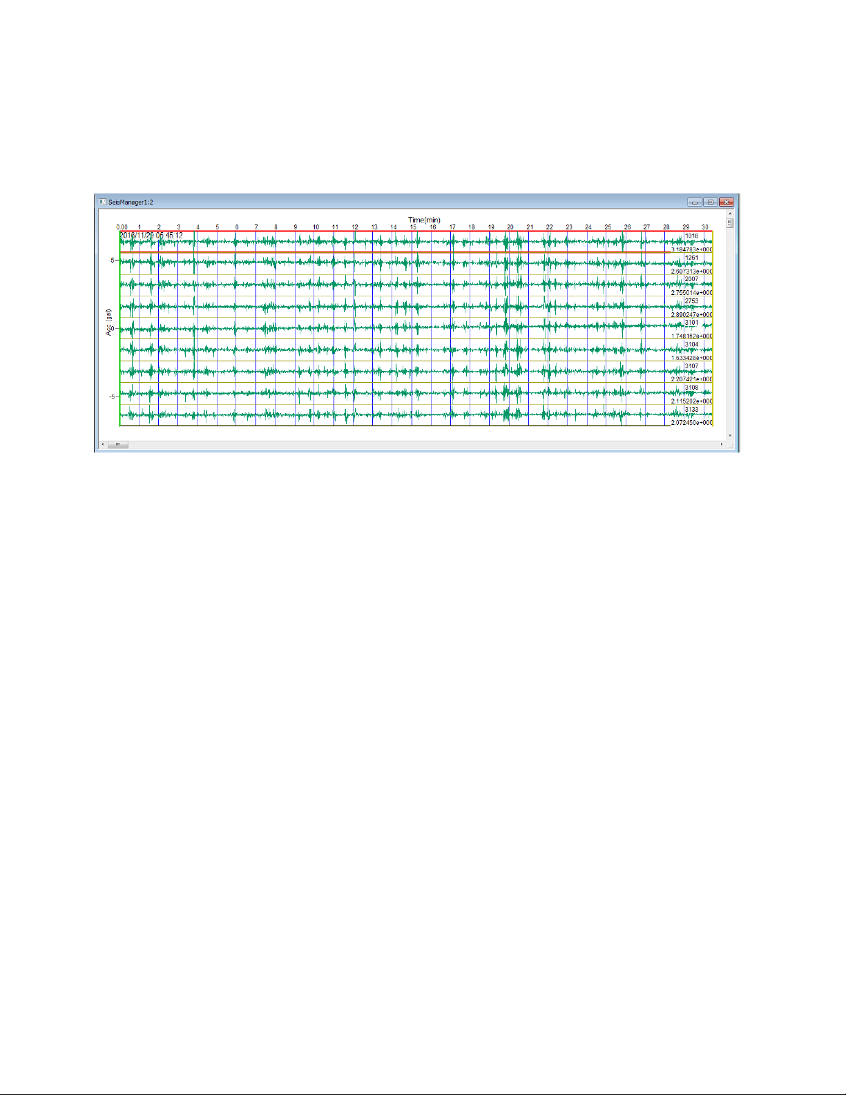
1) Data processing starts from a CTB. Select a CTB to be processed just like exporting waveform data

described in previous section.

Figure 15.3 Example of Common Time Block (CTB).

37

02/06/2019, Rev. 1.6

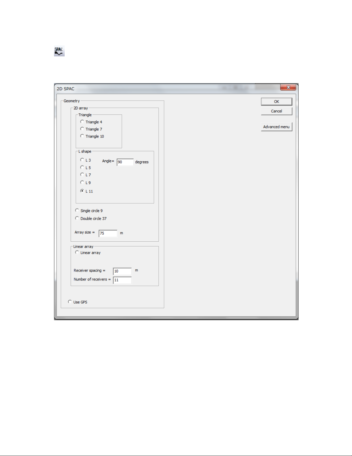
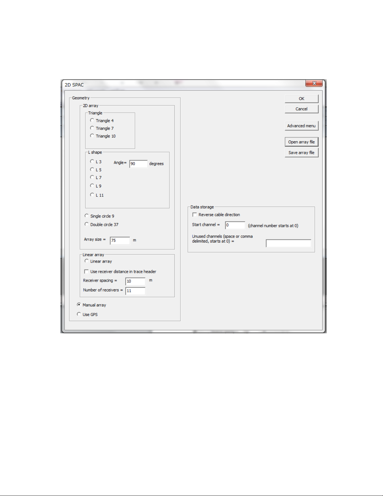
2) Click or select [Analysis]>>[SPAC analysis] to process passive surface wave data in terms of Spatial

Auto Correlation (SPAC). A dialog appears for setting the shape and size of the array. Check “Use GPS” if

GPS location is used for SPAC processing.

Figure 15.4 Dialog box for setting array shape and size.

38

02/06/2019, Rev. 1.6

To view other options, click [Advanced menu]. To use a custom array configuration, click [Open array file]>>

and select an ASCII file containing X-Y location of sensors. Make sure [Manual array] is checked on if you

opened an Array file.

Figure 15.5 Dialog box for setting custom configurations.

39

02/06/2019, Rev. 1.6

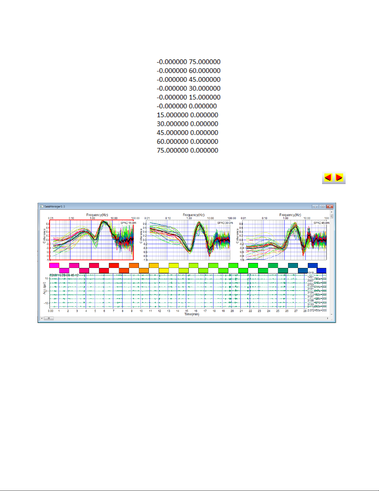
An example of array file is shown below:

3) Spatial auto correlations appear. When number of receiver separation is more than three, use

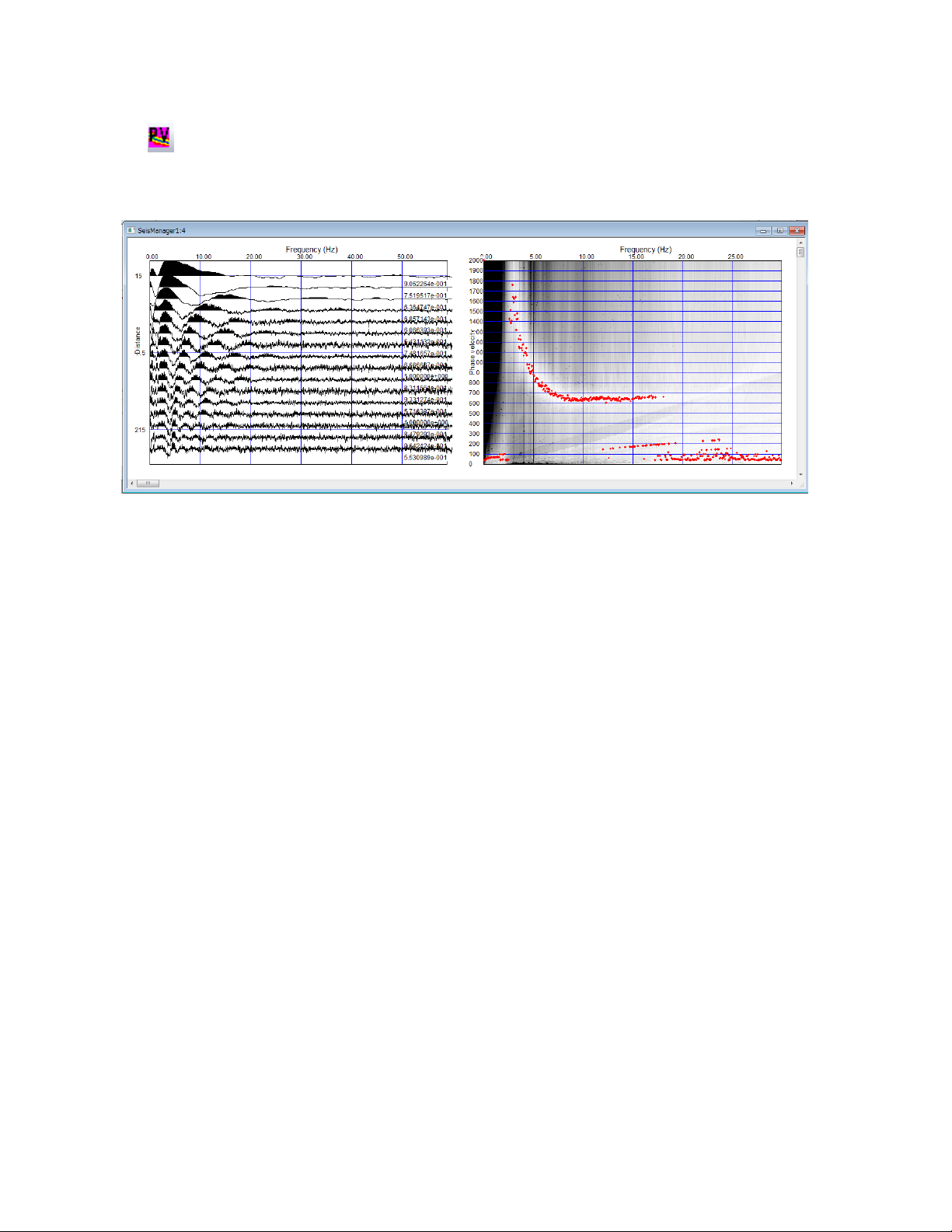
buttons to scroll receiver separations to be shown.

4) Optional : Select [File]>>[Save SPAC data as SEG2 file] to save all spatial auto-correlations into a SEG2

file. Use Pickwin to process saved SEG2 files.

Figure 15.6 Spatial auto correlations.

40

02/06/2019, Rev. 1.6

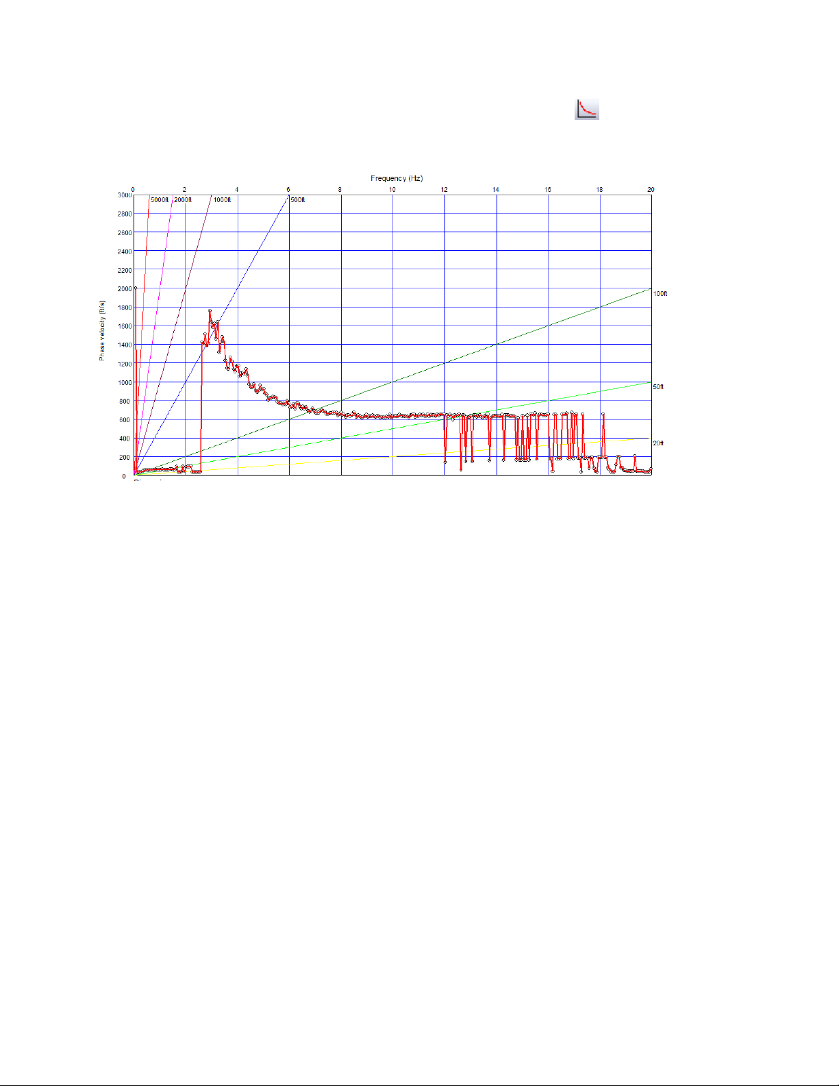
5) Click or select [Phase velocity analysis]>>[Phase velocity window] and all spatial auto-correlations

and a frequency domain phase velocity image appear in another window.

6) Optional : Use [Surface wave analysis]>>[Set up phase velocity image] to change the configuration (min.

and max. phase velocities etc.) of the phase velocity image and picking.

Figure 15.7 Phase velocity image and dispersion curves.

41

02/06/2019, Rev. 1.6

7) To launch WaveEQ and display dispersion curves on your display, click or select [Surface wave

analysis]>>[Show phase velocity curve(s)] >>[Launch WaveEq].

Figure 15.8 Dispersion curve with phase velocity

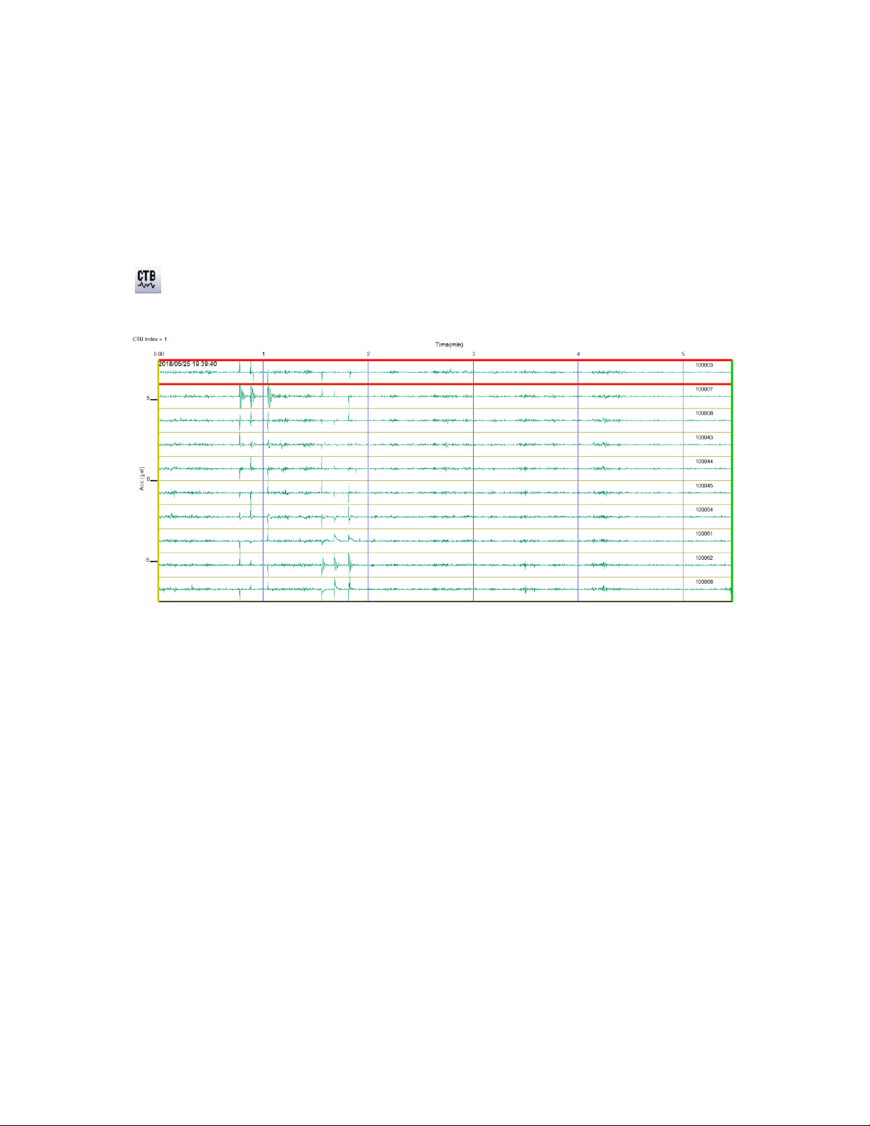
42

02/06/2019, Rev. 1.6

16. Basic active data processing using SPACPlus and Pickwin in SeisImager.

Acquisition parameter for active survey is the same as typical passive recording (4 ms sampling and 12 db

gain). Data acquisition does not need a trigger. Make sure all Atom units are recording and swing a hammer

or drop a weight at the appropriate shot location. It is better to note a number of shots, location and

approximate time of each shots.

1) Click or select [Window]>>[Processing window] and the selected CTB data (in a red rectangle) will

appear in another window.

Figure 16.1 Active data from the Common Time Block.

43

02/06/2019, Rev. 1.6

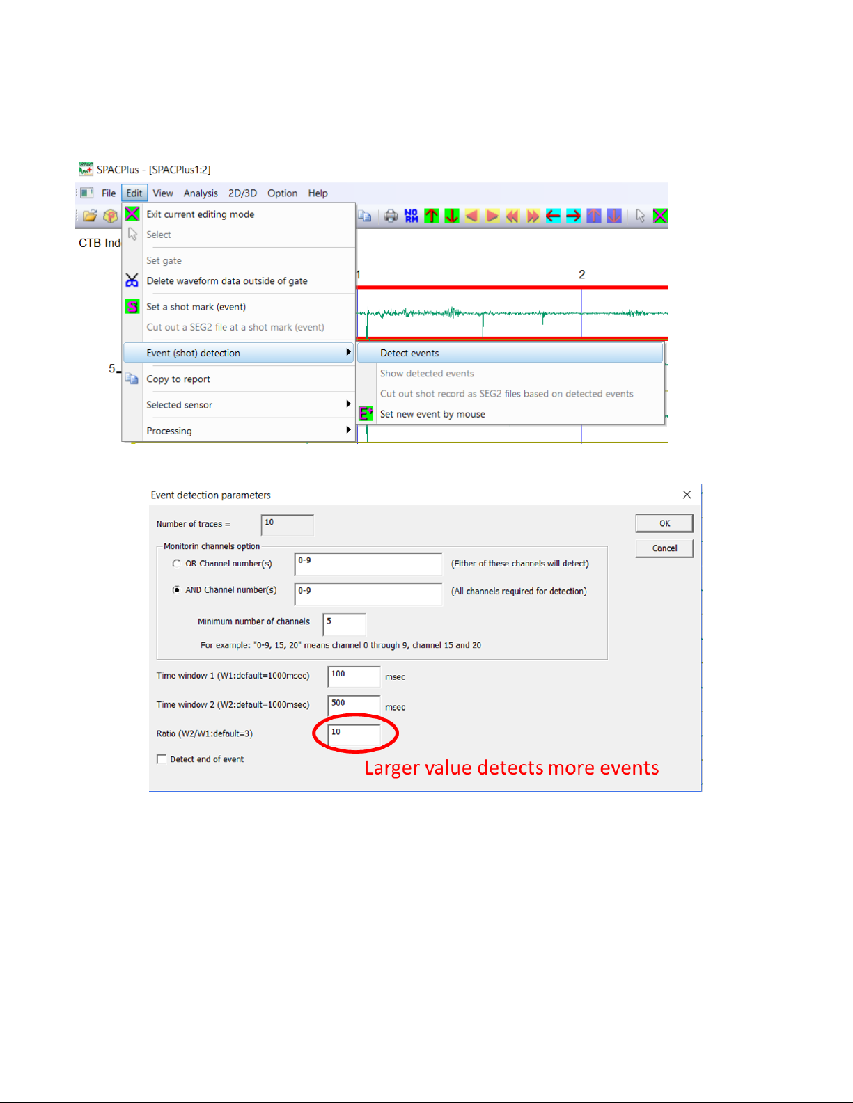
2) To detect shots (events), select [Edit]>>[Event (shot) detection]>>[Detect events] and set event detection

parameters.

Figure 16.2 Example of parameters for event detection.

44

02/06/2019, Rev. 1.6

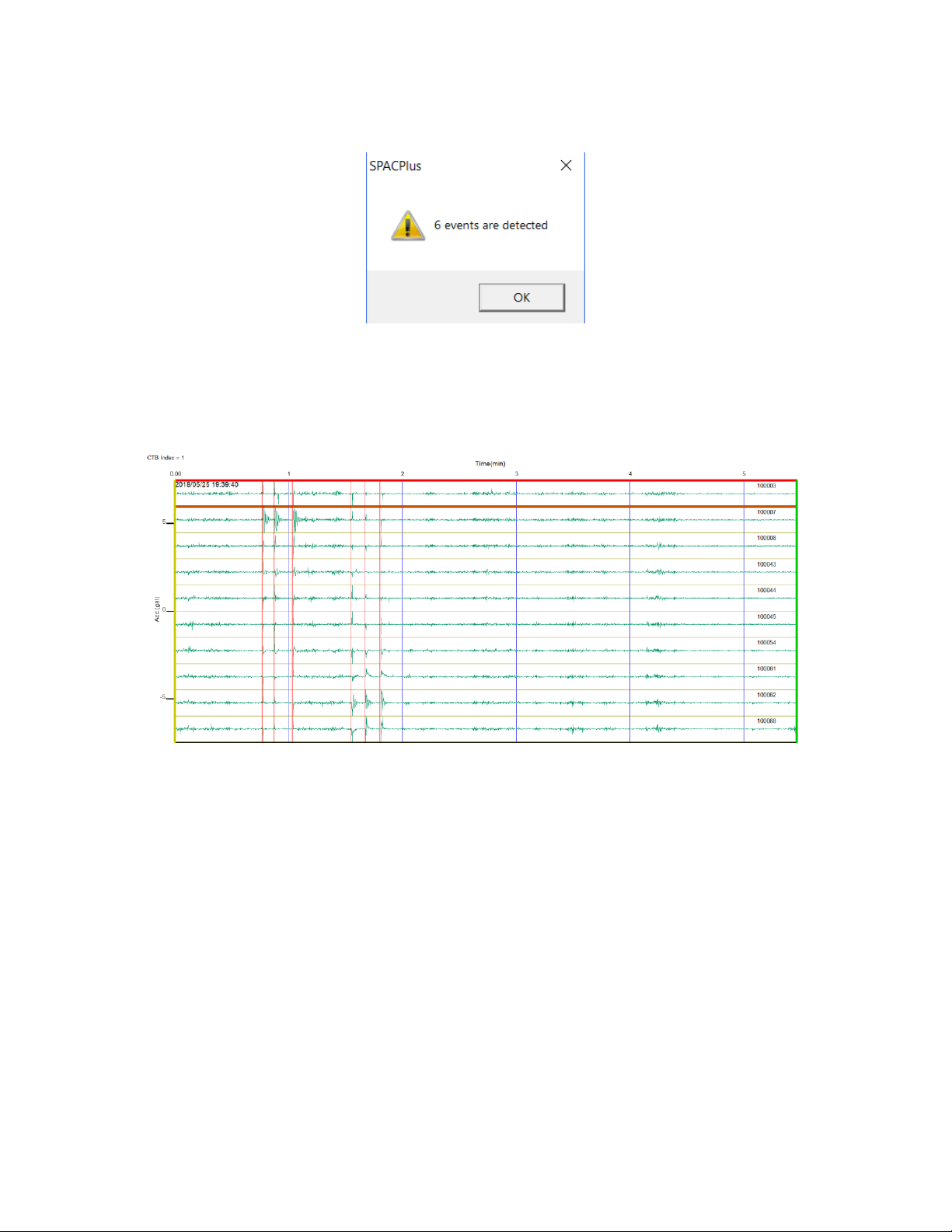
3) Number of detected events appears.

4) Detected events (shots) are shown as red lines. Adjust the settings and repeat the detection until
appropriate detections were obtained.

Figure 16.3 Detected events (shots).

45

02/06/2019, Rev. 1.6

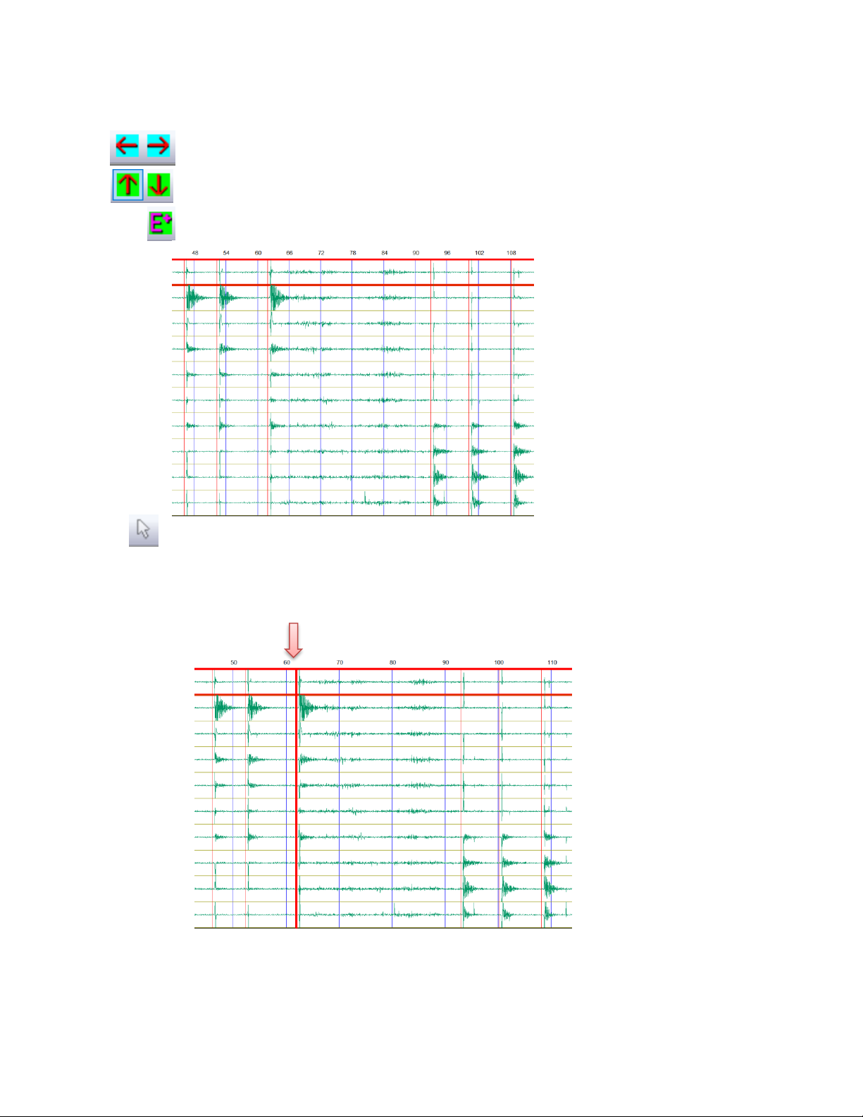
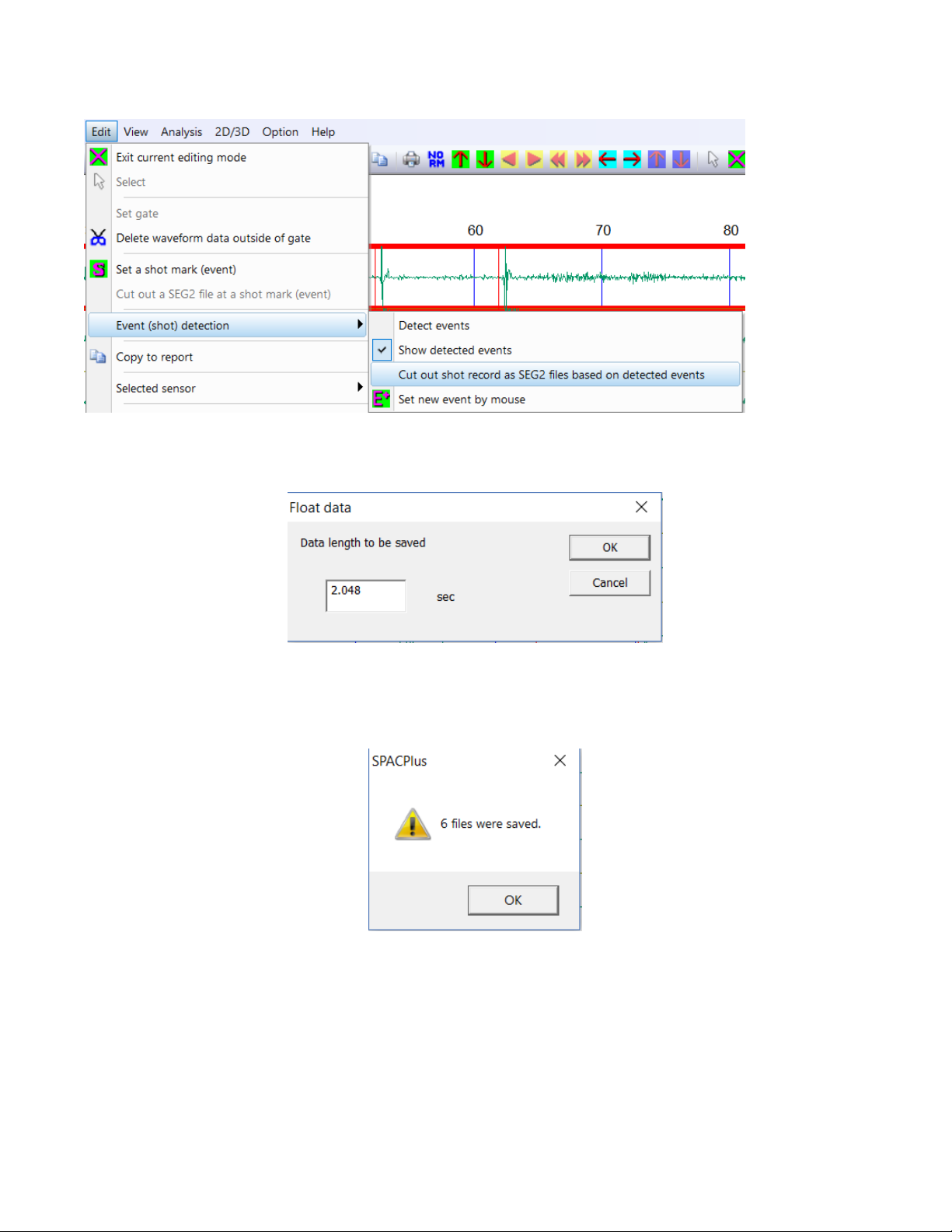
5) Detected shots can be edited as shown below.

6) To show detected shots by Pickwin, select [Edit]>>[Event (shot) detection]>>[Cut out shot record as
SEG2 files based on detect events].

Use to select a detected event. Selected event is shown as a red bold

line. Hit delete key to delete the detected event. Use a mouse to move the

event (left button down).

Change horizontal (time) scale.

Change display amplitude.

Use to Add new event (shots) by clicking a left button of a mouse.

Selected event

46

02/06/2019, Rev. 1.6

Enter data length of shot records to be cut out.

Number of saved shot record files appears.

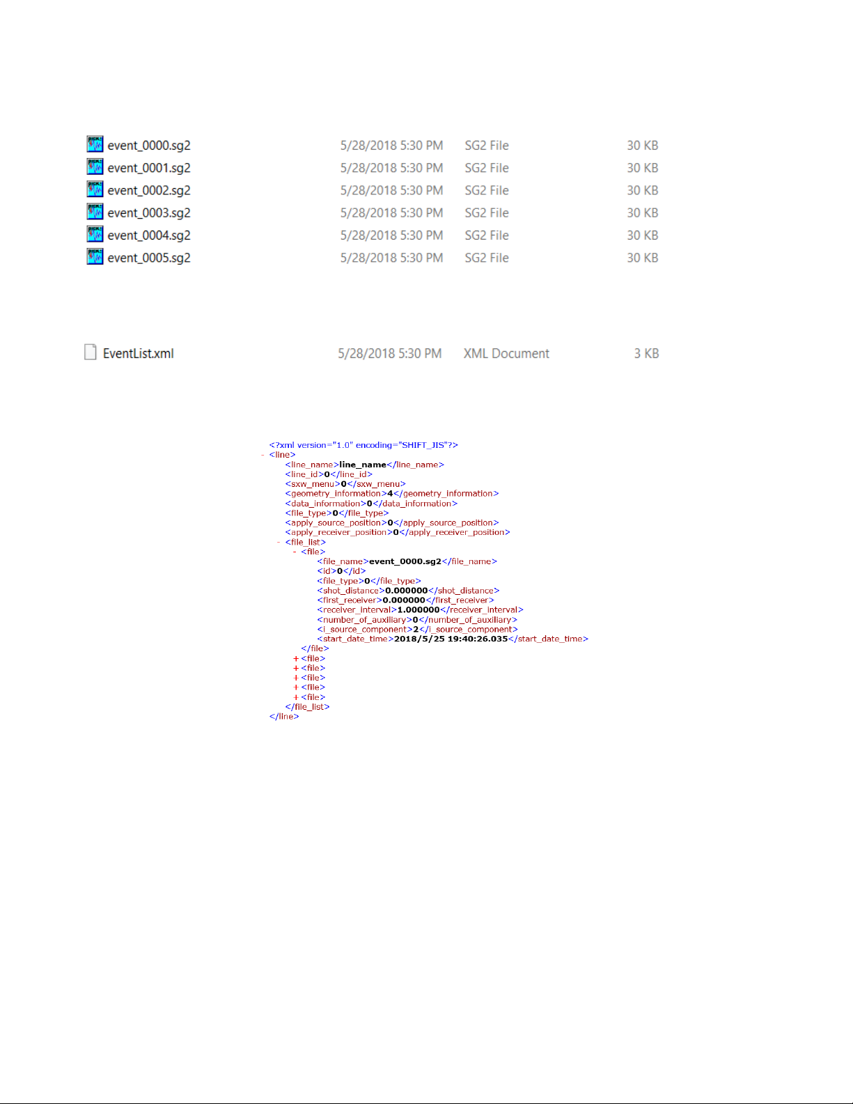
47

02/06/2019, Rev. 1.6

The shot record files were saved as SEG2 files (.sg2) in a folder being selected.

A file list was saved in an XML file in the same folder.

The XML file contains a list of shot record files.

48

02/06/2019, Rev. 1.6

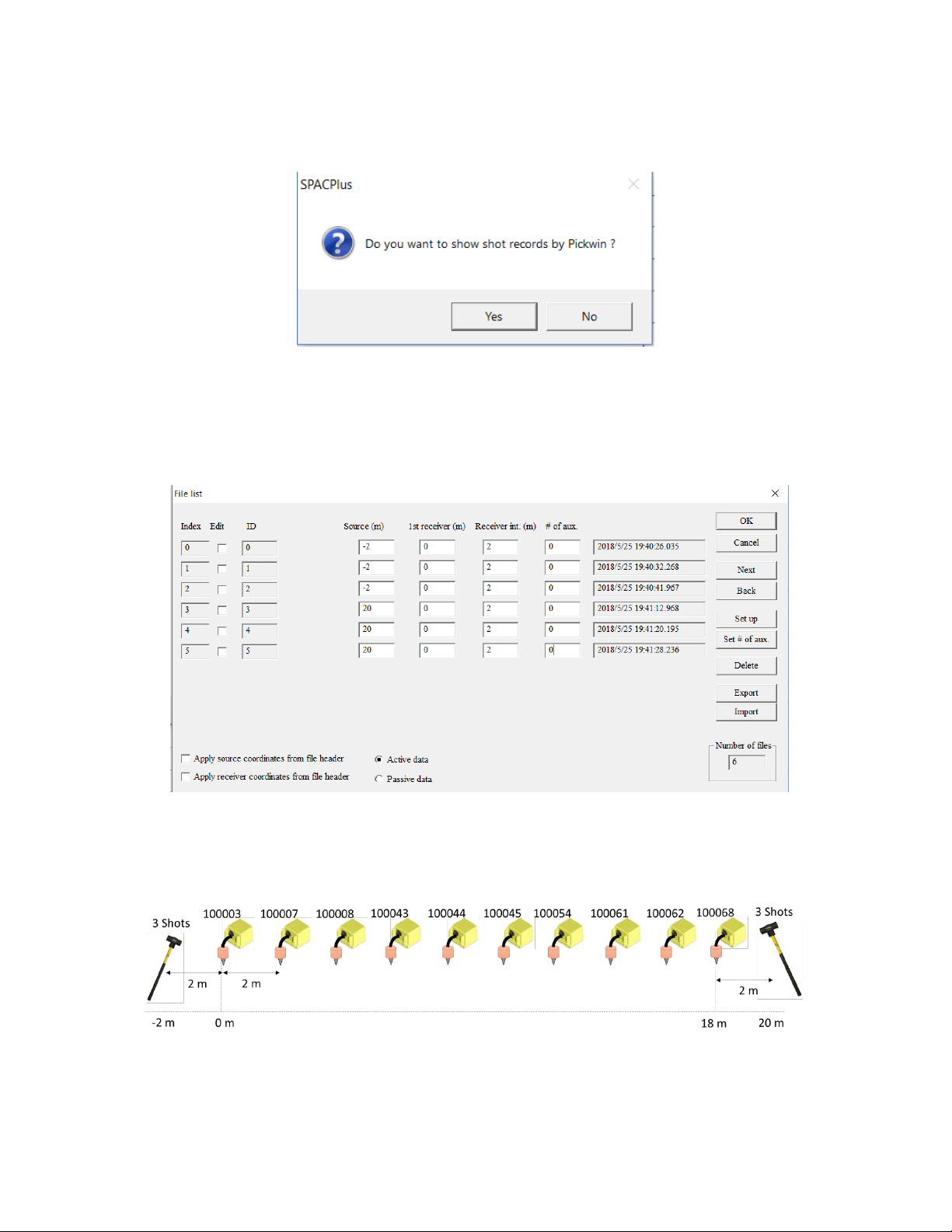
Click “Yes” to launch Pickwin and continue the processing.

7) Pickwin is launched and the list of shot records appear in a dialog box. Set up source location, receiver
interval etc. Figure 14.4 shows the setting for the sample data described in the section 17. Figure 14.5
shows the source-receiver configuration of the sample data corresponding to the Figure 14.4.

Figure 16.4 File list shown by Pickwin.

Figure 14.5 Source-receiver configuration corresponding to the Figure 14.3.

49

02/06/2019, Rev. 1.6

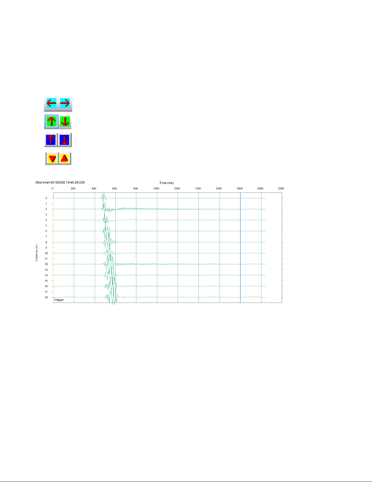
8) Individual shot record shown by Pickwin. This manual describes a data processing of active surface wave
methods from here. General seismic data processing, such as picking first arrival for refraction analysis, is

also possible. See “SeisImager/2DTM Manual” for the detail of refraction processing using SeisImager/2D.

Figure 16.6 Example of individual shot record shown by Pickwin.

Change horizontal (time) scale.

Change amplitude.

Change distance scale.

Scroll shot records.

50

02/06/2019, Rev. 1.6

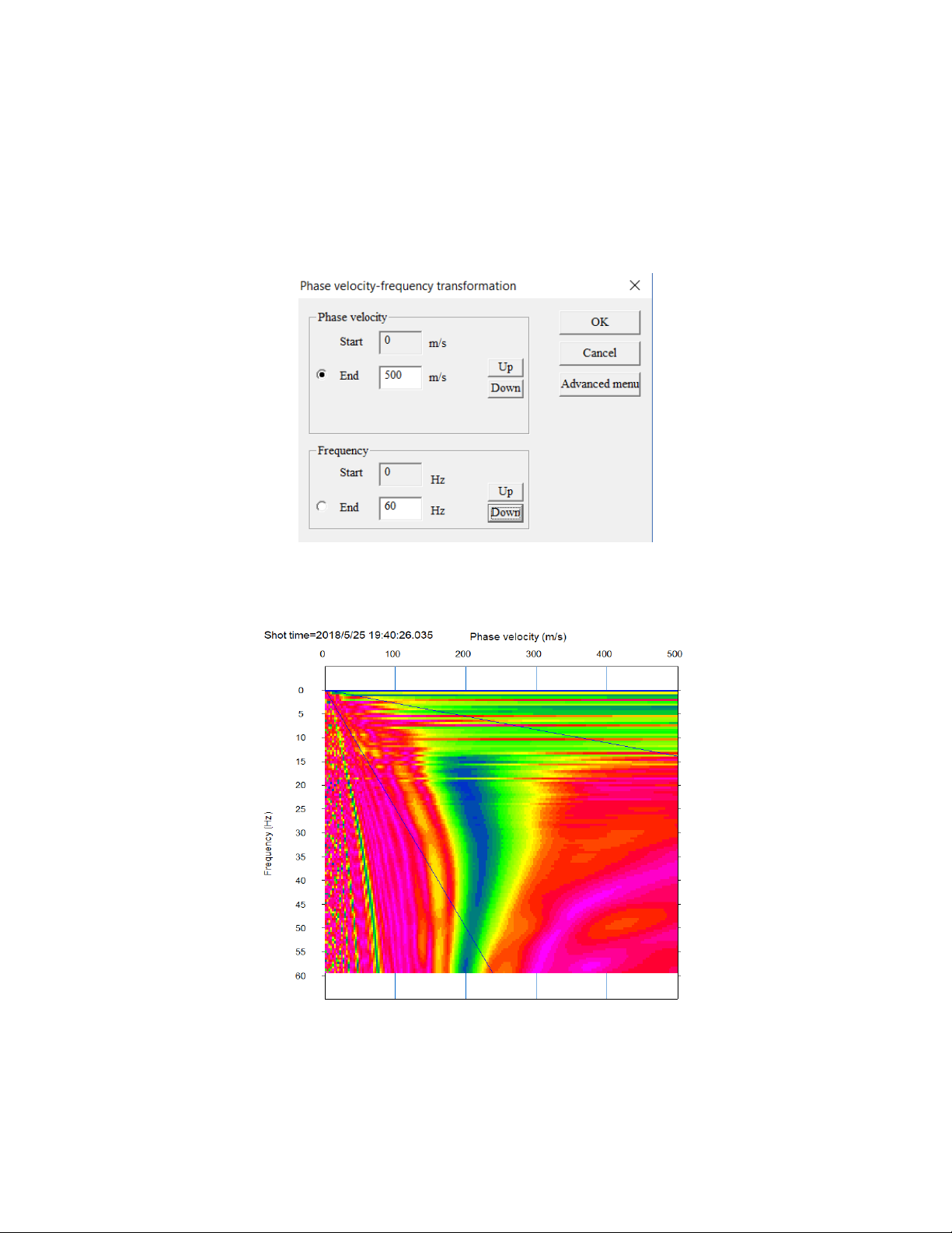
9) To transform time domain waveform data to phase velocity image in frequency domain, select [Surface

wave analysis]>>[Phase velocity frequency transformation] or press “Ctrl+D” to transform data to a phase

velocity image in frequency domain.

Set up max. phase velocity and max. frequency.

A phase velocity image in frequency domain appears.

Figure 16.7 Phase velocity image in frequency domain.

51

02/06/2019, Rev. 1.6

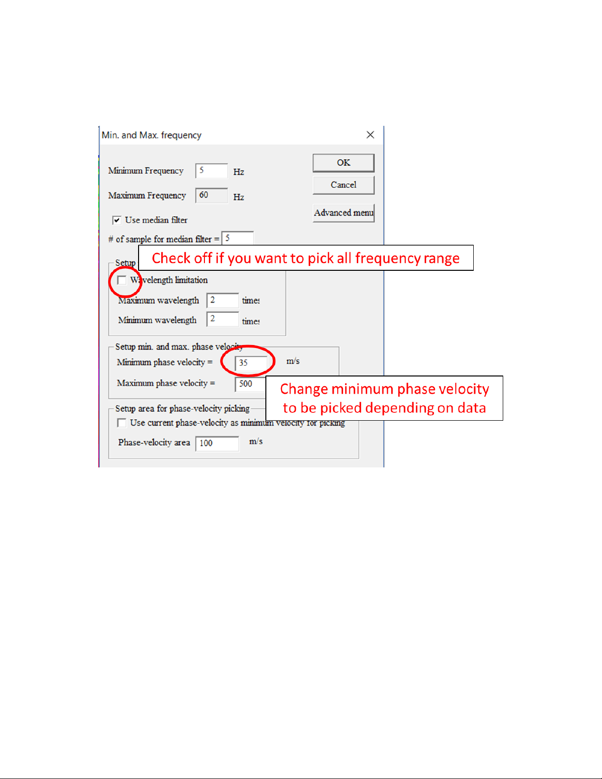
10) To pick phase velocities, Select [Surface wave analysis]>>[Pick phase velocity (1D)] and set up
parameters. Click “Advanced menu” to set up detailed parameters.

52

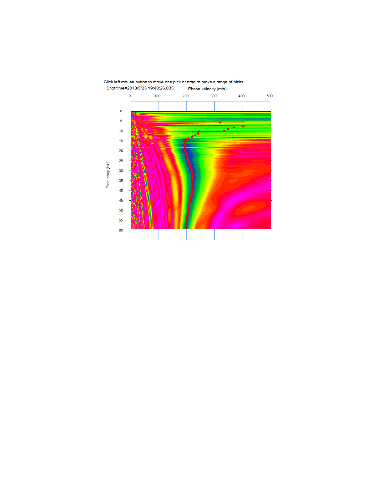
02/06/2019, Rev. 1.6

11) Picked phase velocities appear on a phase velocity image in frequency domain. Click left mouse button
to move one pick or drag to move a range of picks.

Figure 16.8 Picked phase velocities on the phase velocity image in frequency domain.

12) To show a dispersion curve by WaveEq, select [Surface wave analysis]>>[Show phase velocity curve
(1D) <Launch WaveEq>].

53

02/06/2019, Rev. 1.6

17. Combine passive and active surface wave data.

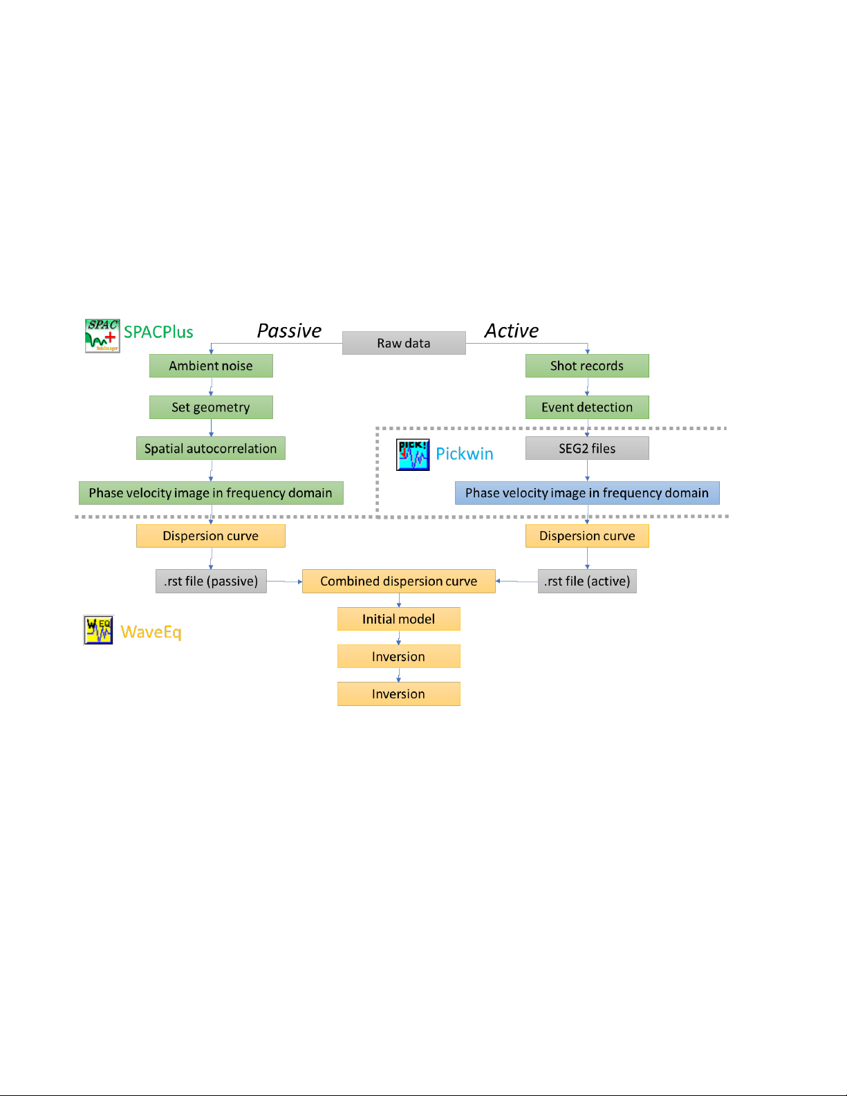
This section briefly summarizes a processing flow of combined analysis of active and passive surface wave

data obtained by Atom after both dispersion curves were picked. See “SeisImager/SWTM Manual”,

“SeisImager/SWTM Manual Addendum (H/V)” and “SeisImager/SW-ProTM Manual” for the general and

detailed analysis of dispersion curves and/or H/V curves. Figure 15.1 shows the processing flow of combined

analysis.

Figure 17.1 Processing flow of passive and active surface wave methods.

54

02/06/2019, Rev. 1.6

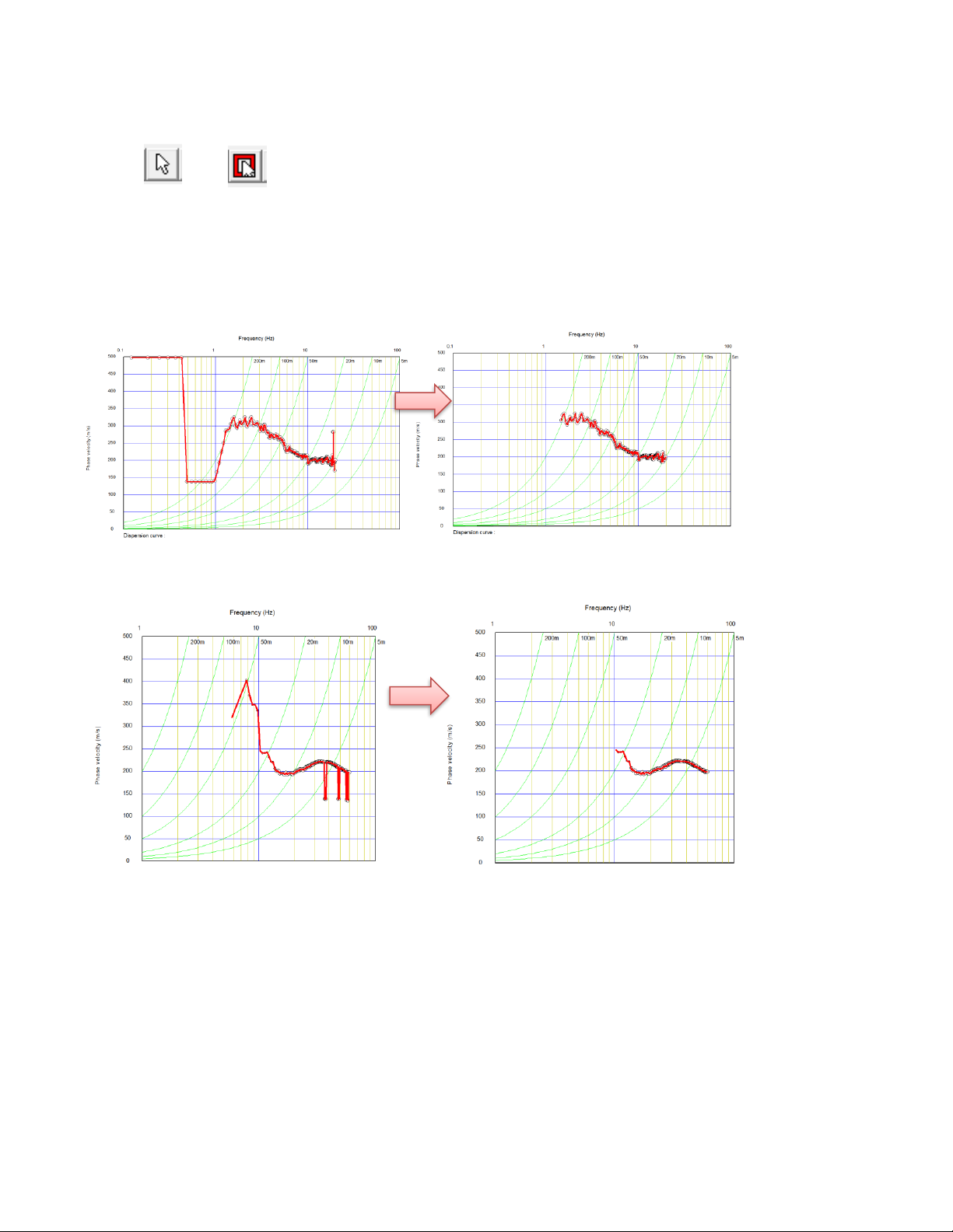
1) Delete noises or unnecessary frequency range.

2) Passive and active dispersion curves must be individually saved as .rst files. To save dispersion curves,

select [File]>>[Save 1D phase velocity curve or H/V curve (.rst)] to save a dispersion curve to data file.

Use or to select phase velocities

Select [Dispersion curves]>>[Delete picks outside of gate] or Ctrl+X to set

unnecessary frequency range.

Hit delete key to delete the selected phase velocities.

Figure 17.2 Examples of dispersion curve editing.

Passive data :

Active data :

55

02/06/2019, Rev. 1.6

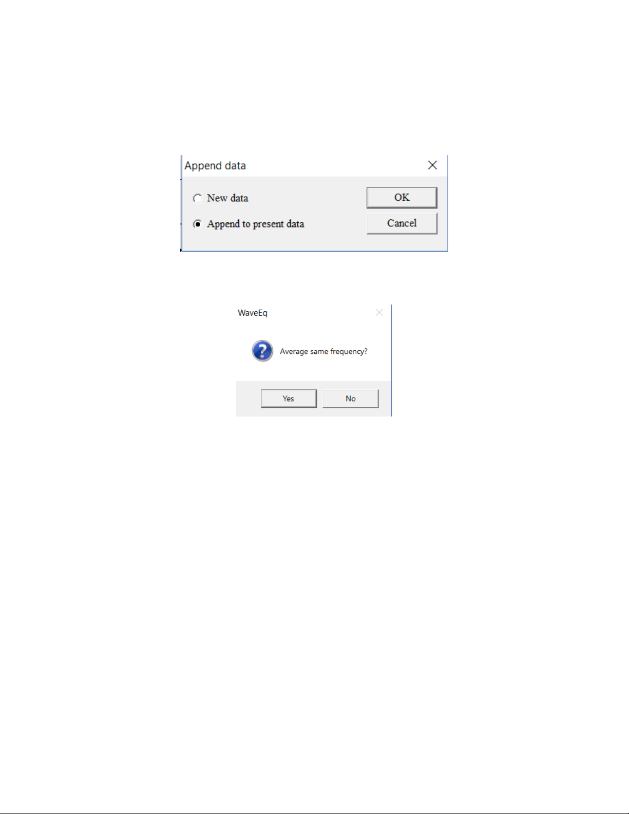
3) To combine active and passive dispersion curves, open one of two files by [File]>>[Open 1D phase

velocity curve or H/V curve (.rst)]. Then open another file [File]>>[Open 1D phase velocity curve or H/V

curve (.rst)]. and choose “Append to present data”.

Data will be automatically averaged if “Yes” is chosen. Choose “No” if you want do not want to average

automatically.

56

02/06/2019, Rev. 1.6

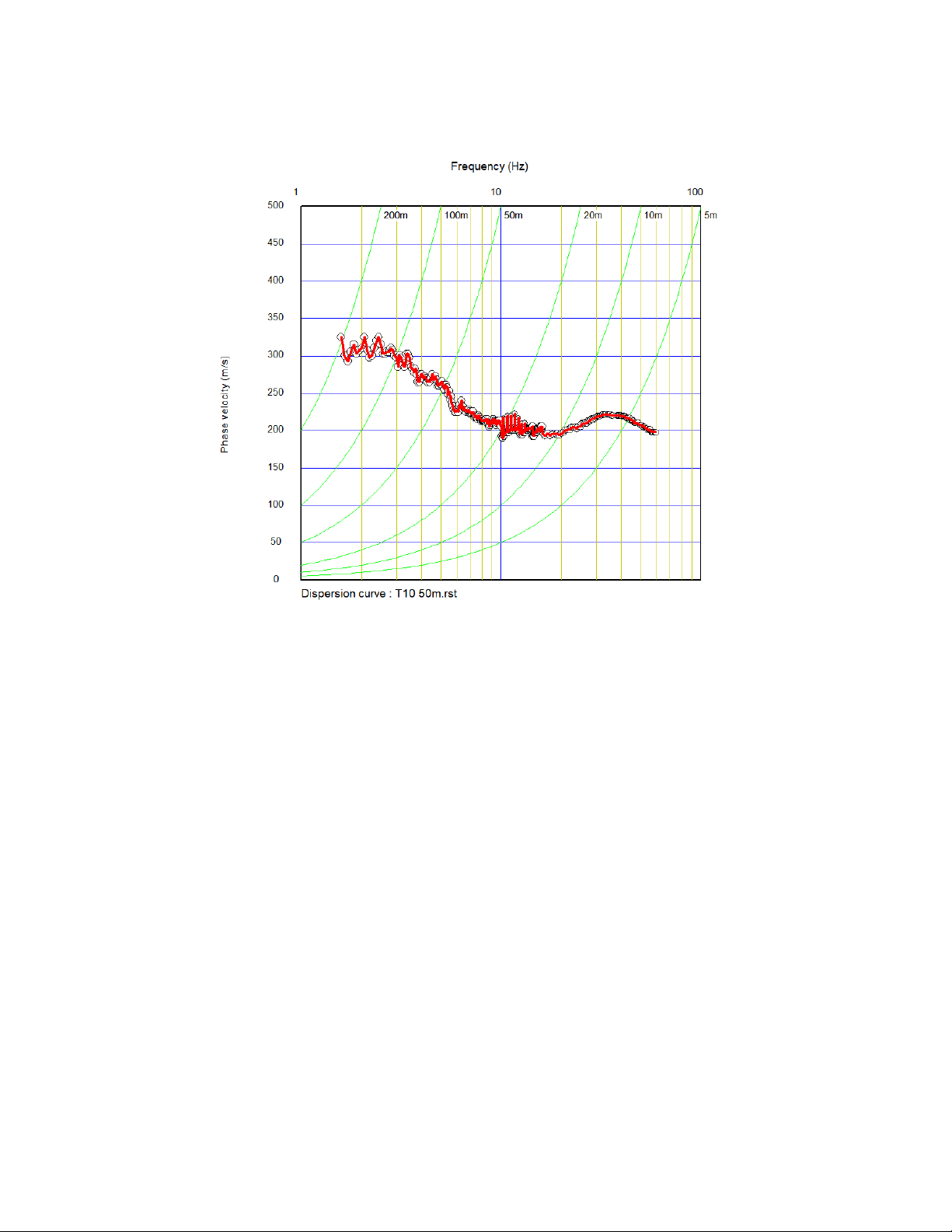
Active and passive phase velocities are shown together.

Figure 17.3 Active and passive dispersion curves.

57

02/06/2019, Rev. 1.6

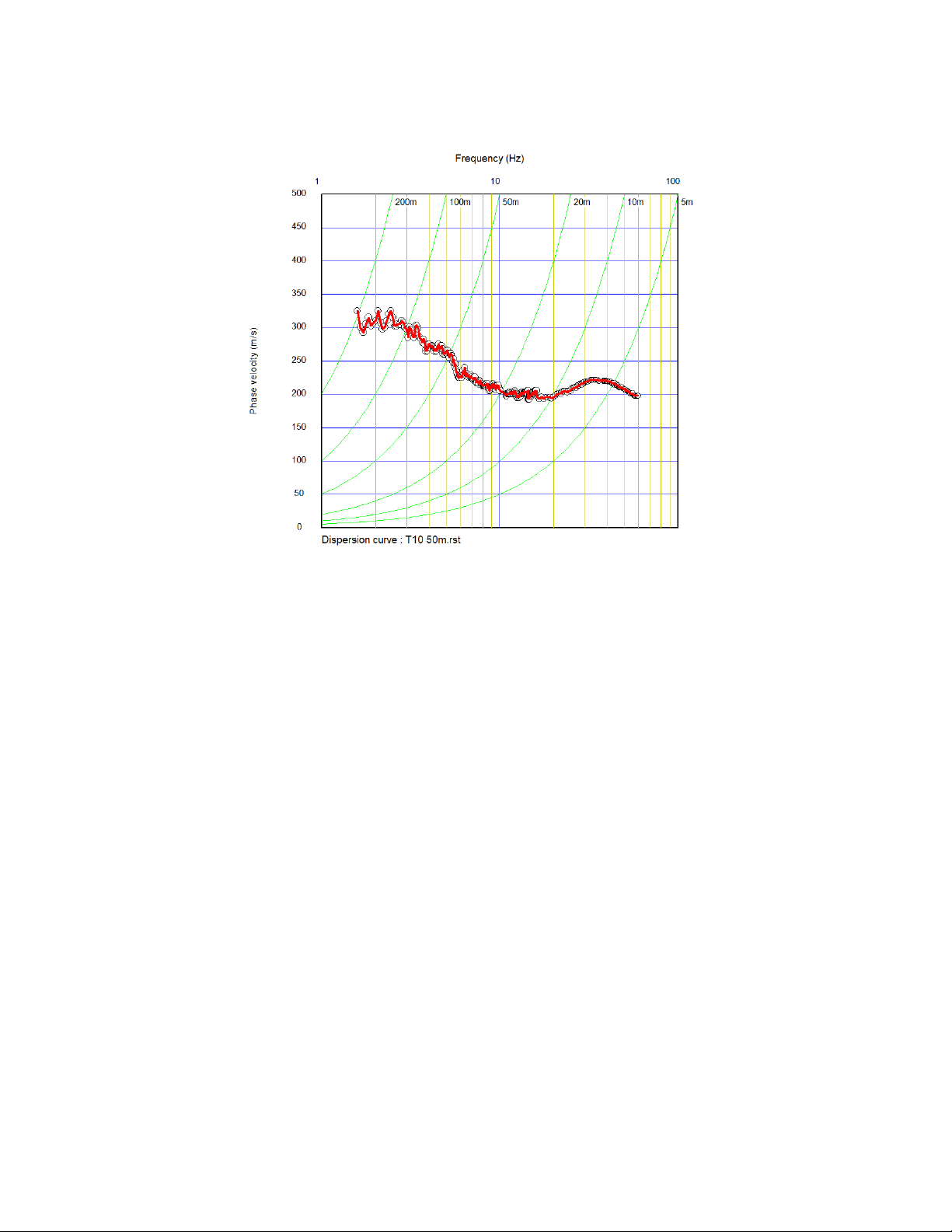
4) Edit active and passive dispersion curves to delete noises or unnecessary frequency range.

Figure 17.4 Edited dispersion curves.

58

02/06/2019, Rev. 1.6

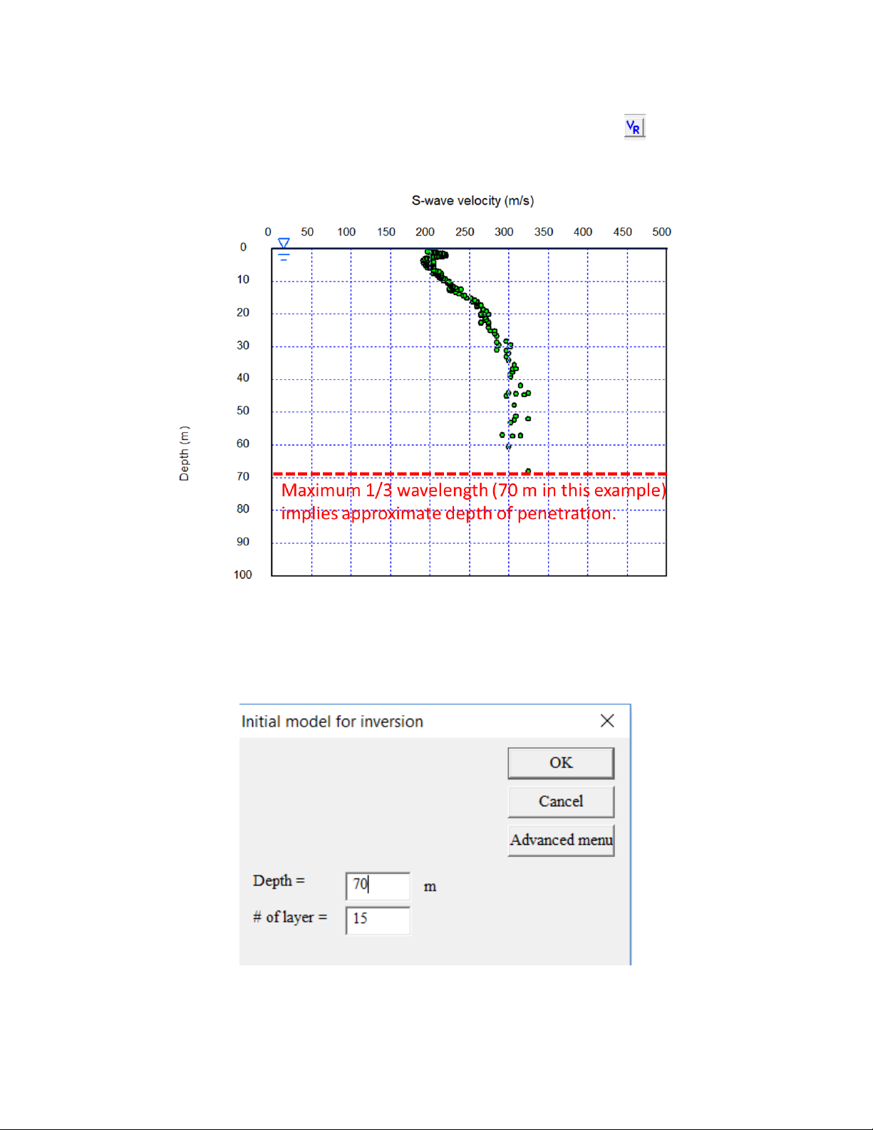
5) It is better to inspect penetration depth before generating an initial model. Crick to evaluate

approximate depth of penetration. Green circles indicate 1/3 wave length.

Figure 17.5 1/3 wavelength implies approximate depth of penetration.

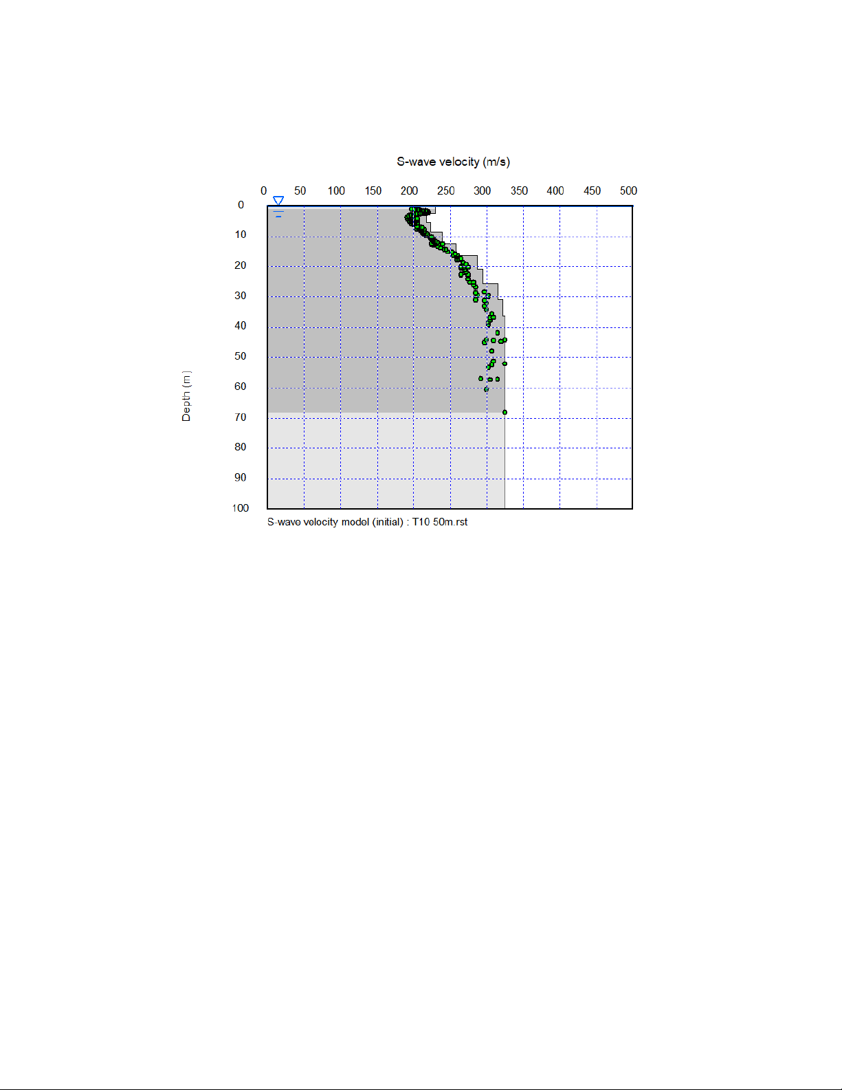
6) To generate initial model, select [Surface wave analysis]>>[MASW (1D)]>>[Initial model] to built an initial

model. Set “Depth” based on a penetration depth implied by 1/3 wave length for example.

59

02/06/2019, Rev. 1.6

7) Refer “SeisImager/SWTM Manual” and “SeisImager/SW-ProTM Manual” for the inversion of dispersion

curves from this point.

Figure 17.6 Example of initial model.

60

02/06/2019, Rev. 1.6

18. Huddle test

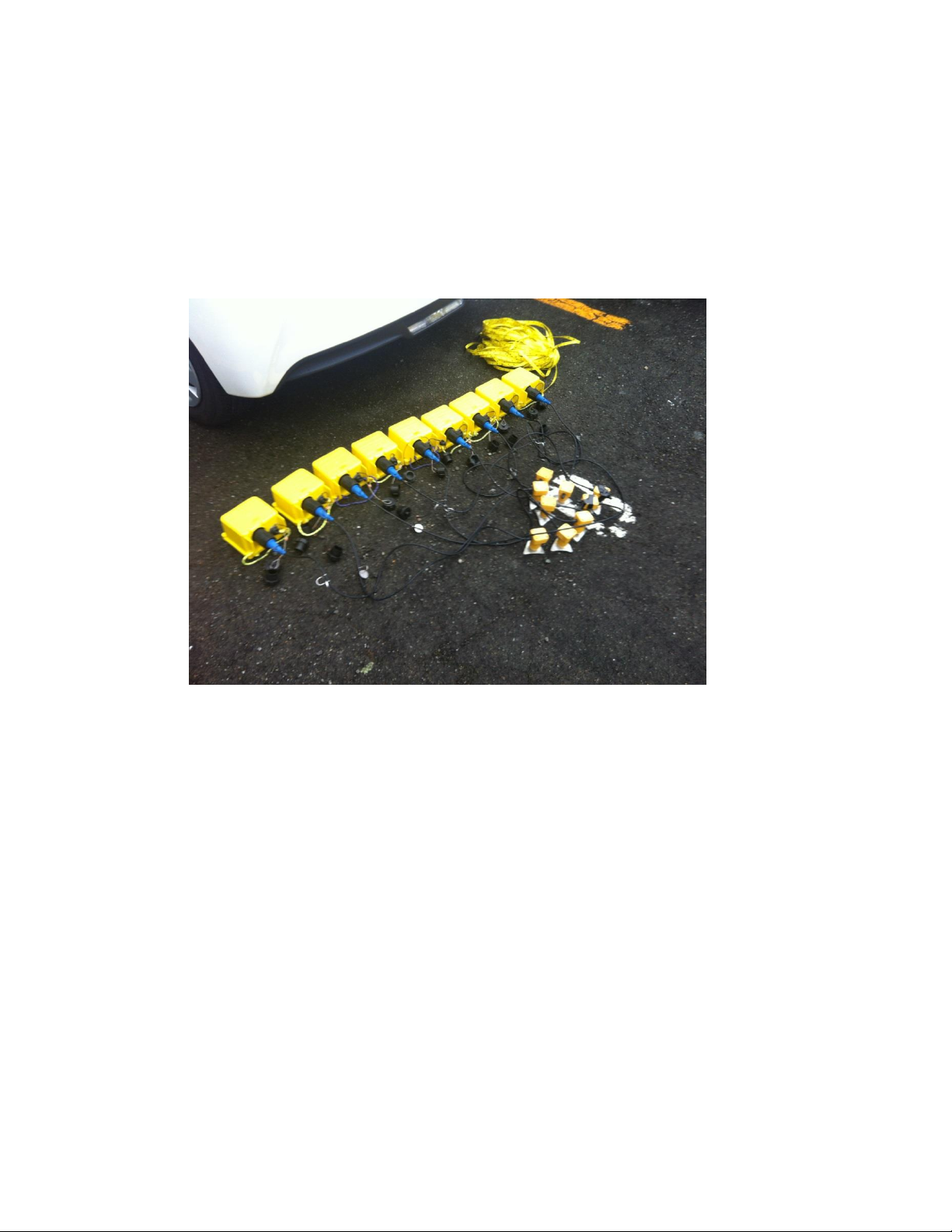
A huddle test is strongly recommended before starting data acquisition to make sure that the character of

the sensor is identical between all of the Atom units. A procedure of huddle test is summarized below.

1) Put all Atom units at one place as shown in Figure 18.1.

2) Record 10 ~ 15 minutes of ambient noise data.

3) To process huddle test, download data from Atom units and select a common time block (CTB).

Coherencies will be calculated between the trace in the red rectangle and all other traces.

Figure 18.1 Huddle test.

61

02/06/2019, Rev. 1.6

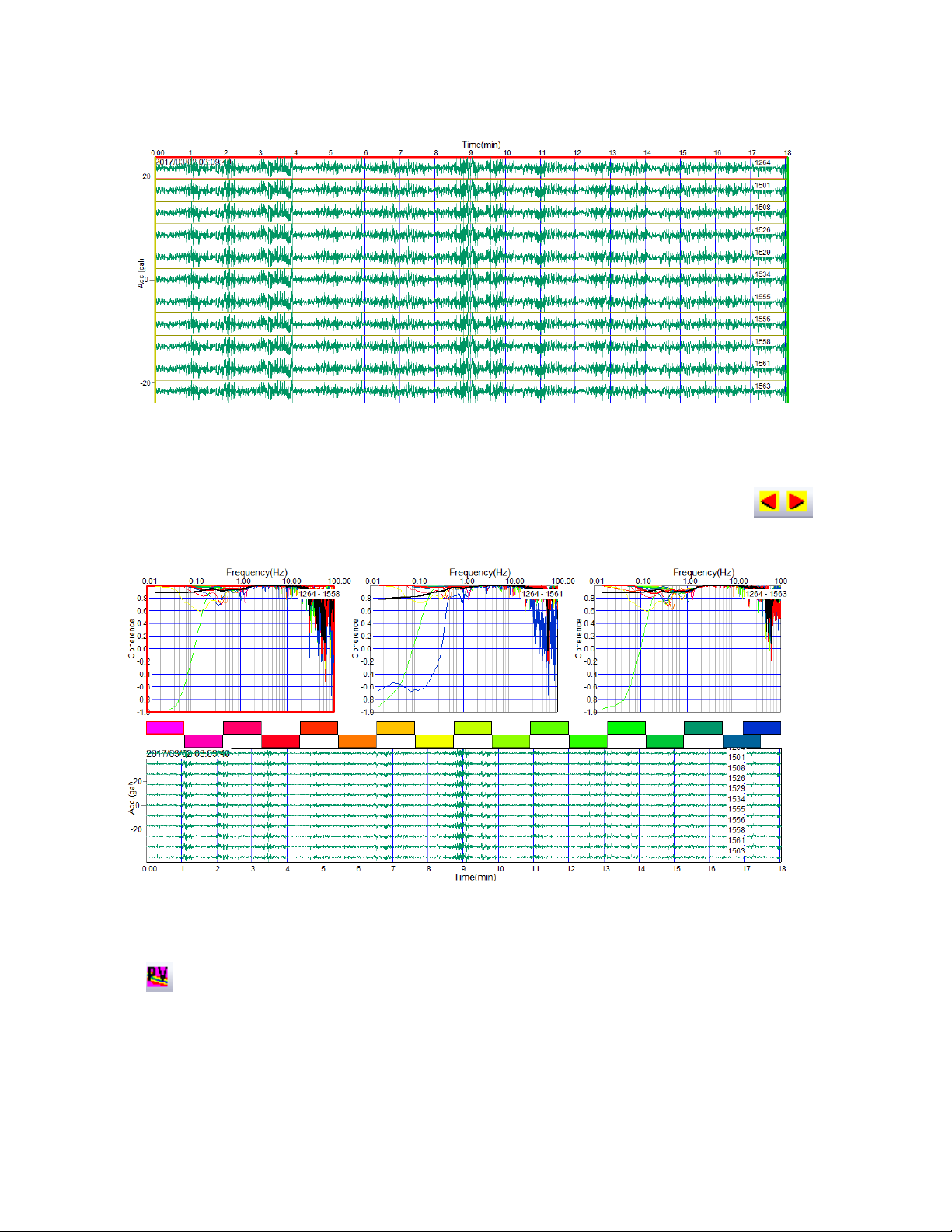
4) Select [Analysis]>>[Coherency analysis] and coherencies appear in another window. Use

buttons to scroll receiver separations to be shown.

5) Click or select [Phase velocity analysis]>>[Phase velocity window] and all coherencies appear in

another window.

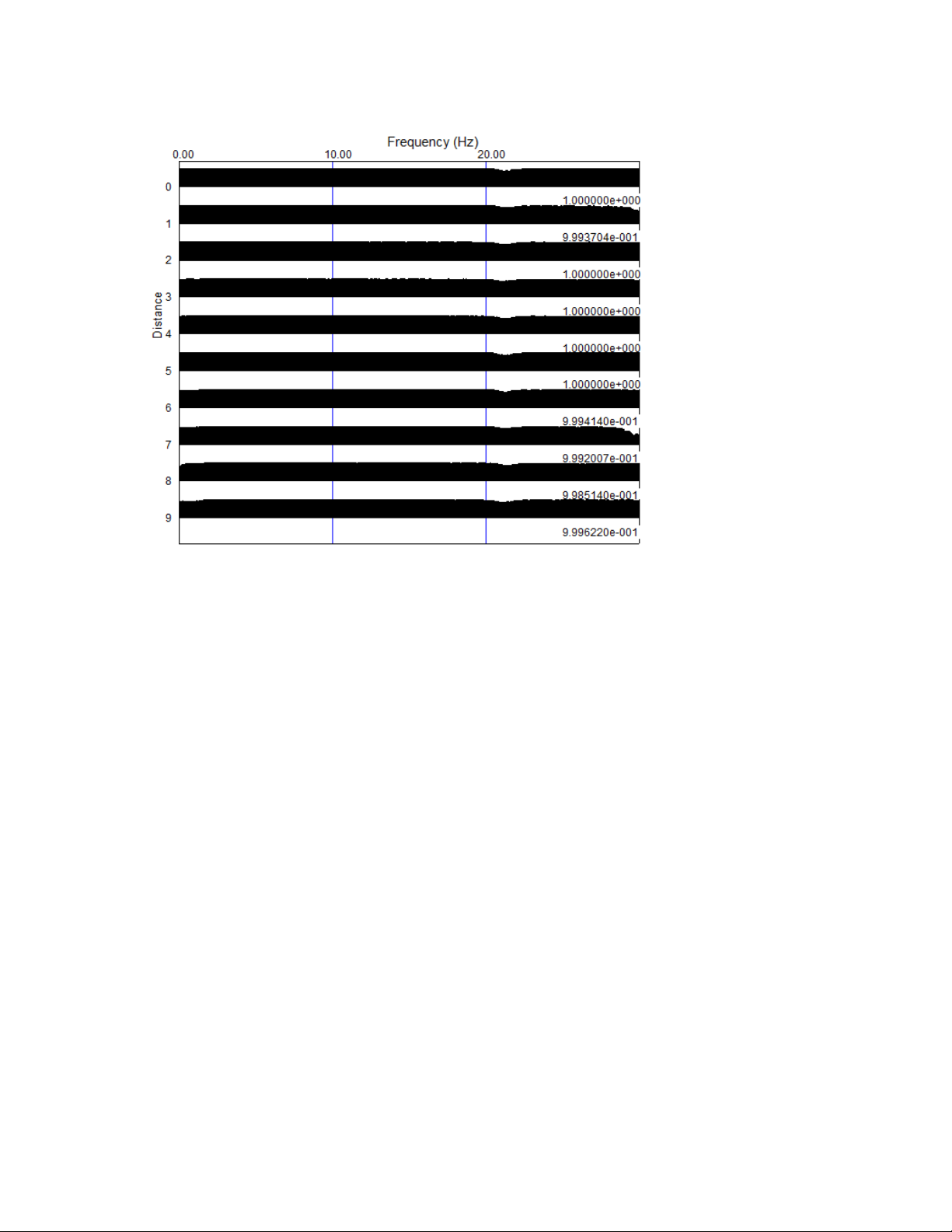
Figure 18.2 Example of ambient noise data for a huddle test.

Figure 18.3 Example of coherencies calculated from huddle test data together

with the raw data.

62

02/06/2019, Rev. 1.6

Figure 18.4 Example of coherencies calculated from huddle test

63

02/06/2019, Rev. 1.6

19. Data example

Data example used in the manual can be downloaded from :

http://seisimager.esy.es/GeophysicalDatabase/t10_50m.zip.

Sample data shown above includes following data.

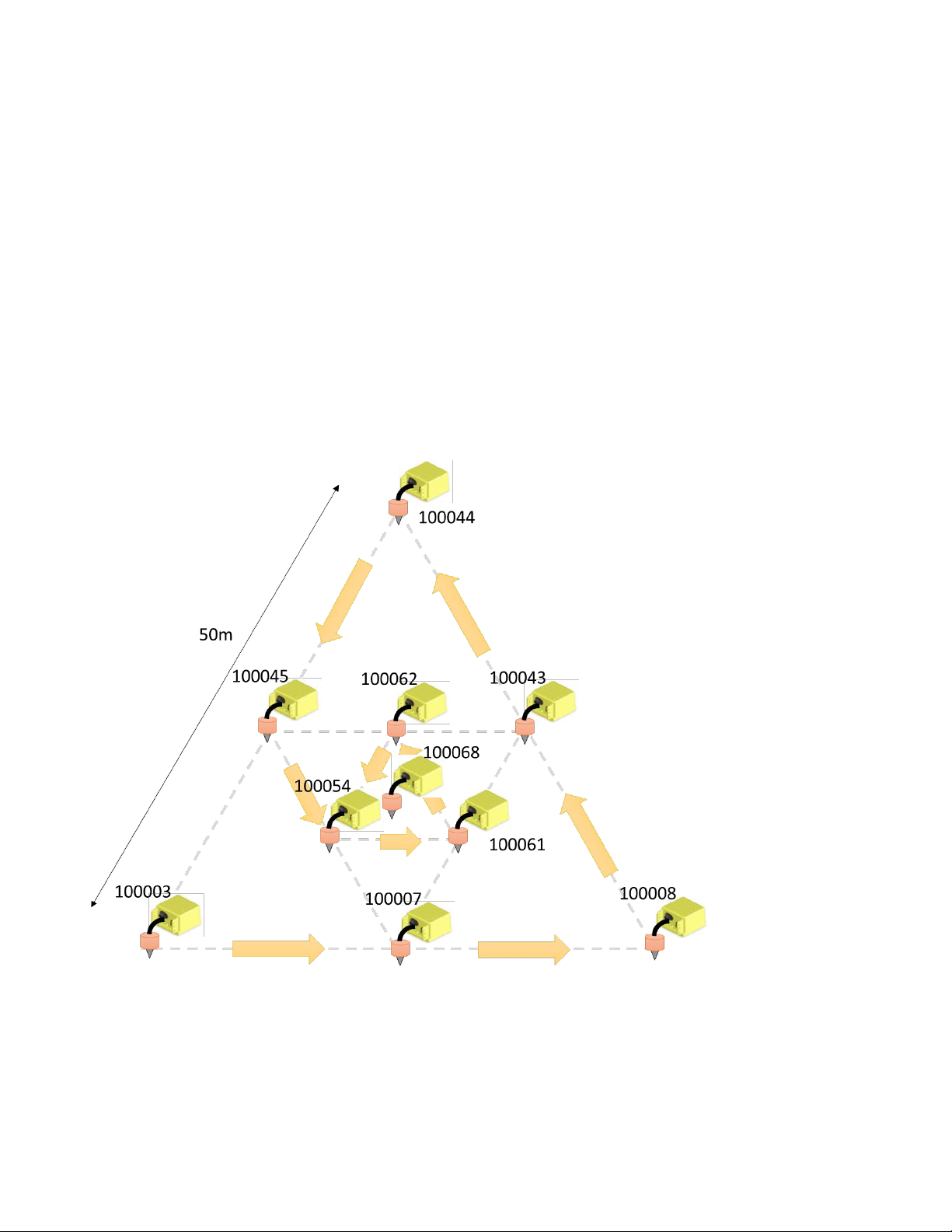
1. Nested triangles of 50 m with 10 receivers recording ambient noise (Figure 17.1).

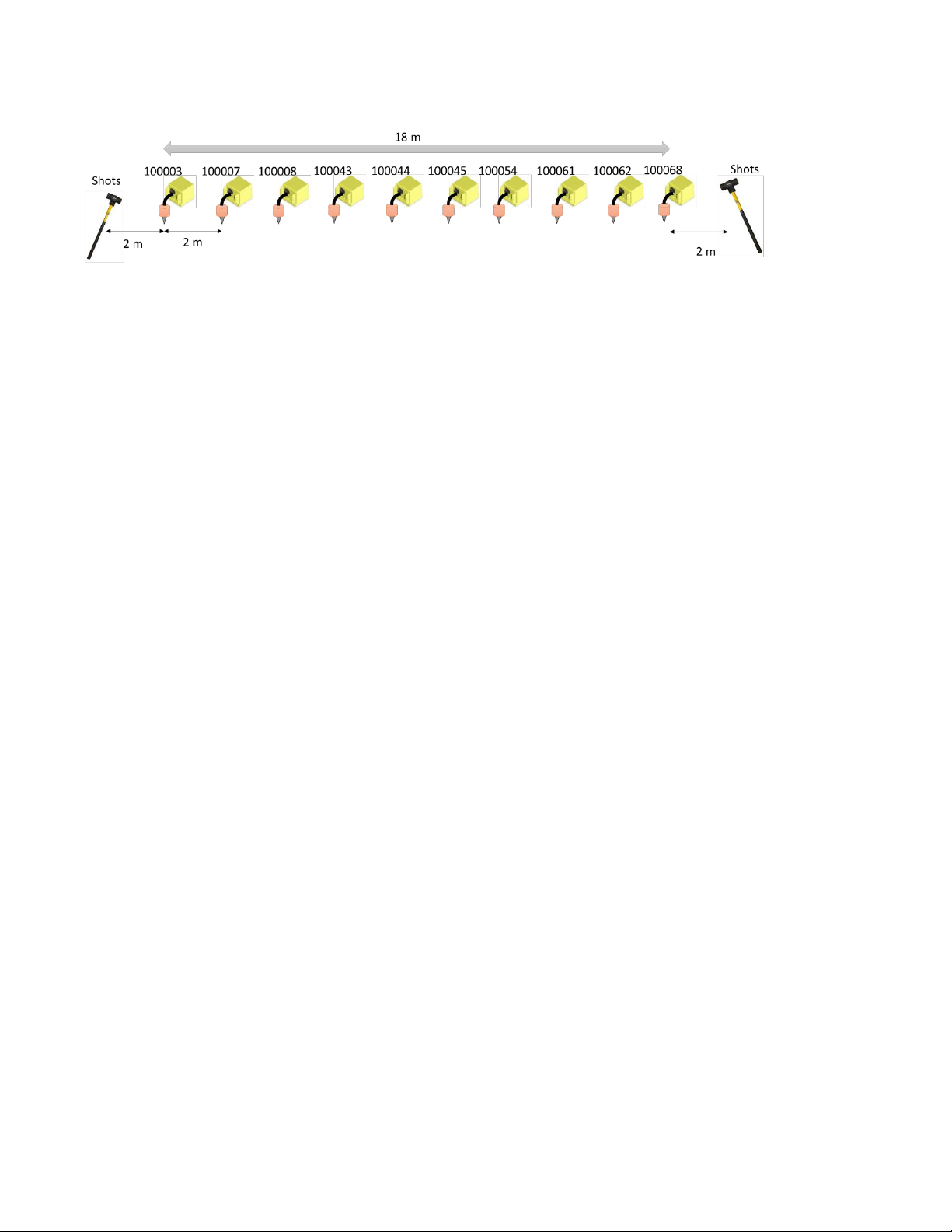
2. Linear array of 10 receivers with 2 m spacings recording active sledge hammer data (Figure 17.2).

3. Linear array of 10 receivers with 2 m spacings recording ambient noise. This measurement is not

necessary.

Figure 19.1 Nested triangles of 10 receivers.

64

02/06/2019, Rev. 1.6

Figure 19.2 Linear array of 10 receivers with 2 m spacings

65

02/06/2019, Rev. 1.6

Appendix A : Confirm or set up the acquisition parameters using SPACPlus

A1) Turn off and stop recording for all Atom units.
A2) Plug in a Wi-Fi access point to your PC. Remove the LAN cable and disable your firewalls and Bluetooth.

A3) Connect your PC’s Wi-Fi to “atom0000”. There should not be “Internet access”.

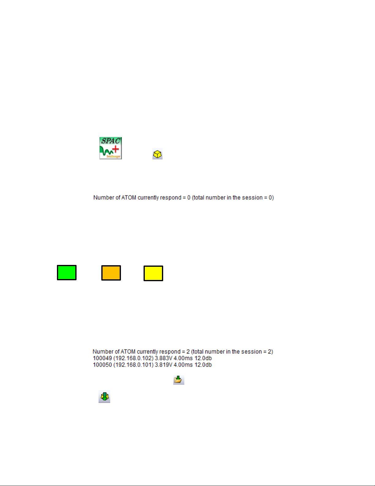
A4) Launch SPACPlus and click or select [File]>>[Atom(Wi-Fi)]>> [Start searching for boxes].

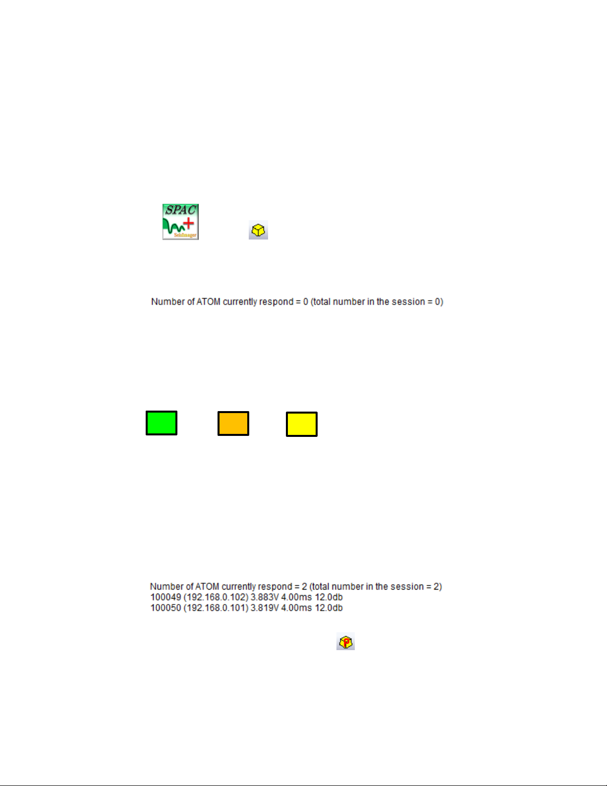
A5) Message shown below appears on the window.

A6) Turn on all Atom units.

The Atom units automatically being download mode when they locate the access point “atom0000”. In

this mode, data recording does not start.

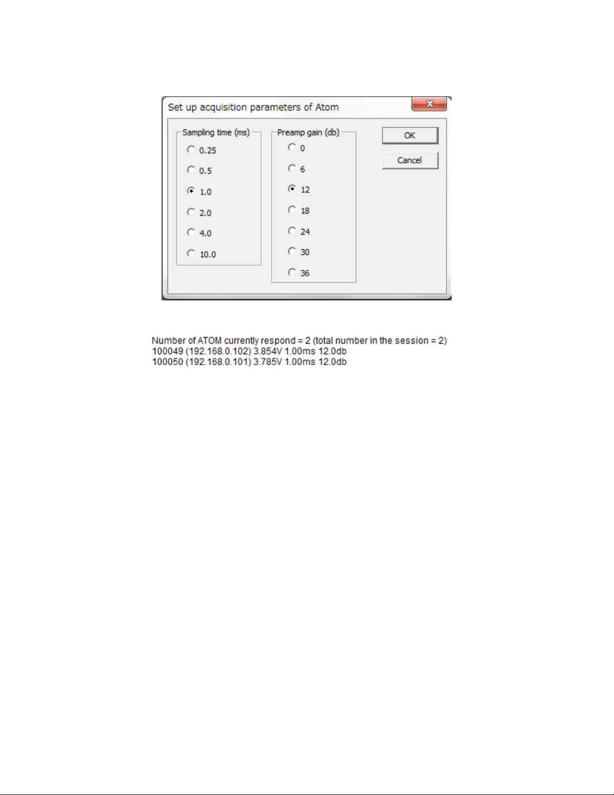
A7) In the SPACPlus window, you will see each Atom units’ ID, IP address, battery voltage, sampling time and

pre-amp gain.Thenumber of Atom units shown in SPACPlus may fluctuate. Note that the default setting of

passive surface wave methods is 4.00 ms and 12.0 db,

A8) To change the Atom unit’s acquisition parameters, click or select [File]>>[Atom (Wi-Fi)]>> [Set up

acquisition parameter].

A9) Select sampling time and preamp gain in a dialog box and click OK.

Battery

Wi-Fi

GPS

Slow Blink.

Slow blink when GPS

is locked.

Blink twice.

Figure 8.1 LEDs when Atom is ready to be controlled from

66

02/06/2019, Rev. 1.6

A10) Confirm changes to the acquisition parameters.

A11) Acquisition parameter can be confirmed or set up via USB using SPACPlus. Use [File]>>[Atom

(USB)]>>[Show Atom AU status] or [Set up acquisition parameter via USB] to confirm or set up acquisition

parameters respectively. To use USB, see Appendix C for more details.

67

02/06/2019, Rev. 1.6

Appendix B : Data download using SPACPlus

B1) Turn off each Atom to stop recording data.

B2) Plug in a Wi-Fi access point to your PC. Remove the LAN cable, turn off your Bluetooth and any firewalls.

B3) Connect your PC’s Wi-Fi to “atom0000”.

B4) Launch SPACPlus and click or select [File]>>[ATOM(Wi-Fi)]>>[Start searching for boxes].

B5) Message shown below appears on the window.

B6) Turn on all Atom units

The Atom units enter download mode when they find the access point named “atom0000”. In this mode, the

data recording does not start.

B7) Atom IDs appear on the window of SeisImager (number of Atom units shown in SeisImager may fluctuate.

B8) Store data into selected directory by clicking or selecting [File]>>[Change destination folder].

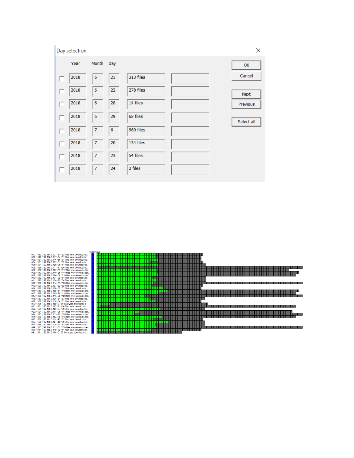
B9) In SPACPlus click or select [File]>>[ATOM(Wi-Fi)]>>[Download folders]. Select the date and time in

hours to download the waveform files.

Battery Wi-Fi

GPS

Slow Blink.

Slow blink when

GPS is locked..

Blink twice.

Figure A.1 LEDs when Atom is ready to download

68

02/06/2019, Rev. 1.6

B 10) Data for multiple dates cannot be downloaded at the same time. Downloaded data have a folder and

file structure shown in 11. Data format.
During the download process,, progress appears on a display similar to the one shown below.

Figure B.1 Selection of data to be downloaded.

Figure B.2 Example of display during download.

69

02/06/2019, Rev. 1.6

Appendix C : Data download using SPACPlus via USB

C1) Insulation of USB driver.
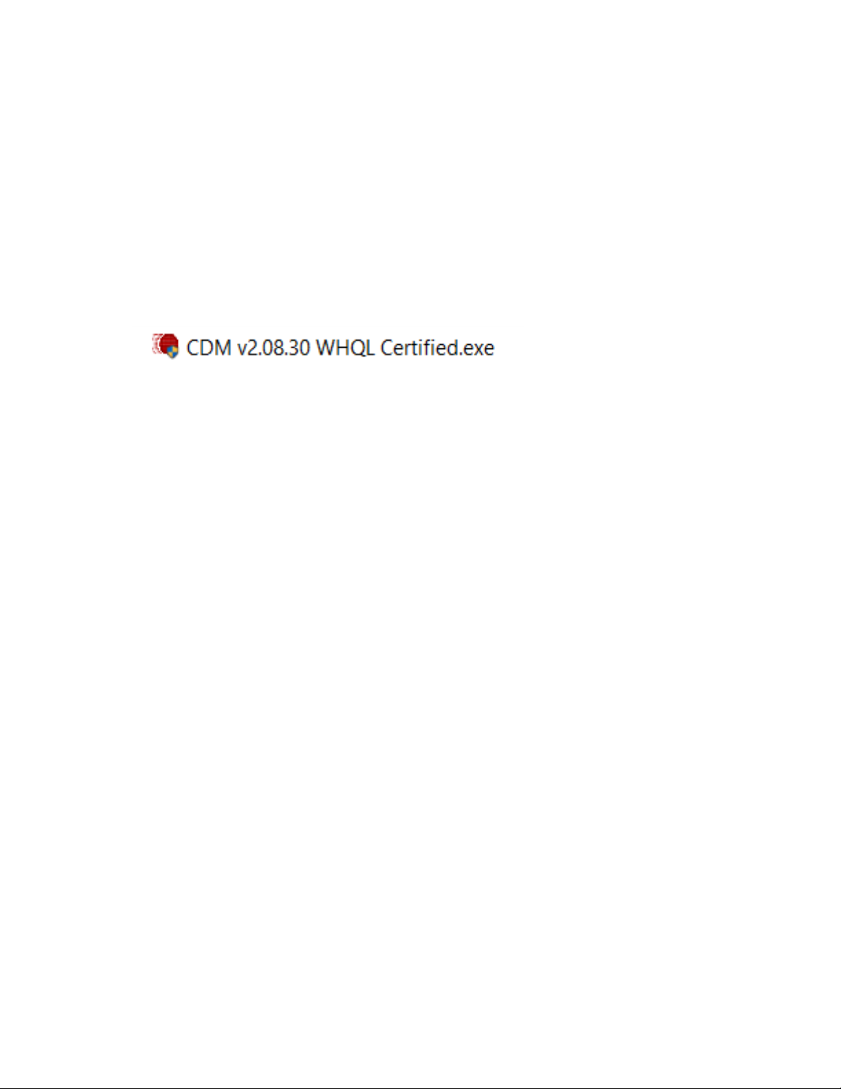
Download USB driver from a link shown below.

https://www.dropbox.com/s/bf38ut5t2ayob8l/CDM_2_08_30.zip?dl=0

Unzip the downloaded file and double click an installer of USB driver.

C2) Find a COM port to be used for Atom

Before downloading data using SPACPlus via USB, comport number to which Atom is connected must be

figured out. There are two ways to fund the comport number.

70

02/06/2019, Rev. 1.6

A) Use SPACPlus

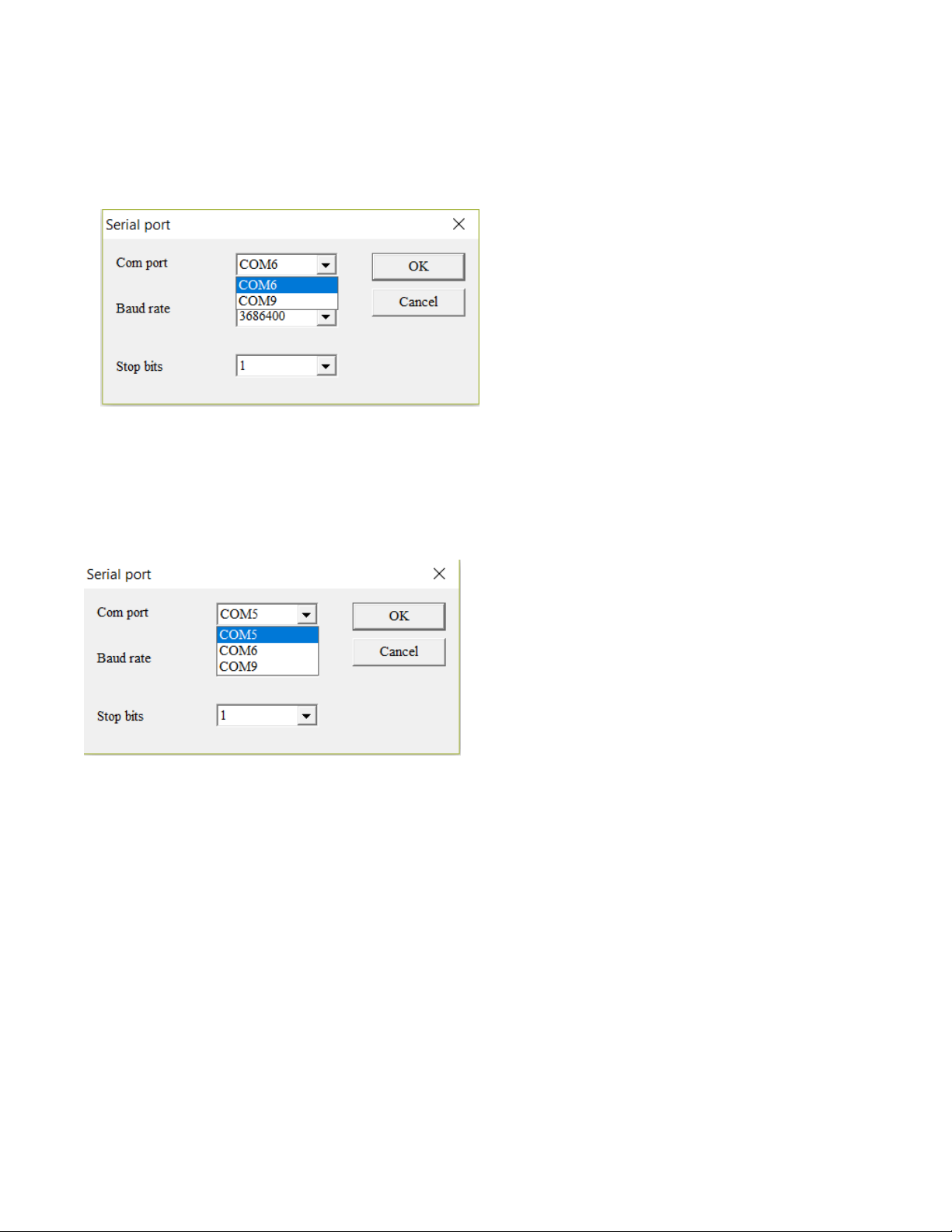
Before connecting Atom to a PC, launch SPACPlus and select [File]>>[Atom (USB)]>>[Show Atom AU status].

A dialog box shows currently available serial ports (COM6 and COM9 in example shown below).

Close SPACPlus.
Connect an Atom to the PC by an USB cable and launch SPACPlus again.

Select [File]>>[Atom (USB)]>>[Show Atom AU status] and new comport (COM5 in example shown below)

indicates the comport number Atom is attached.

71

02/06/2019, Rev. 1.6

B) Use device manager
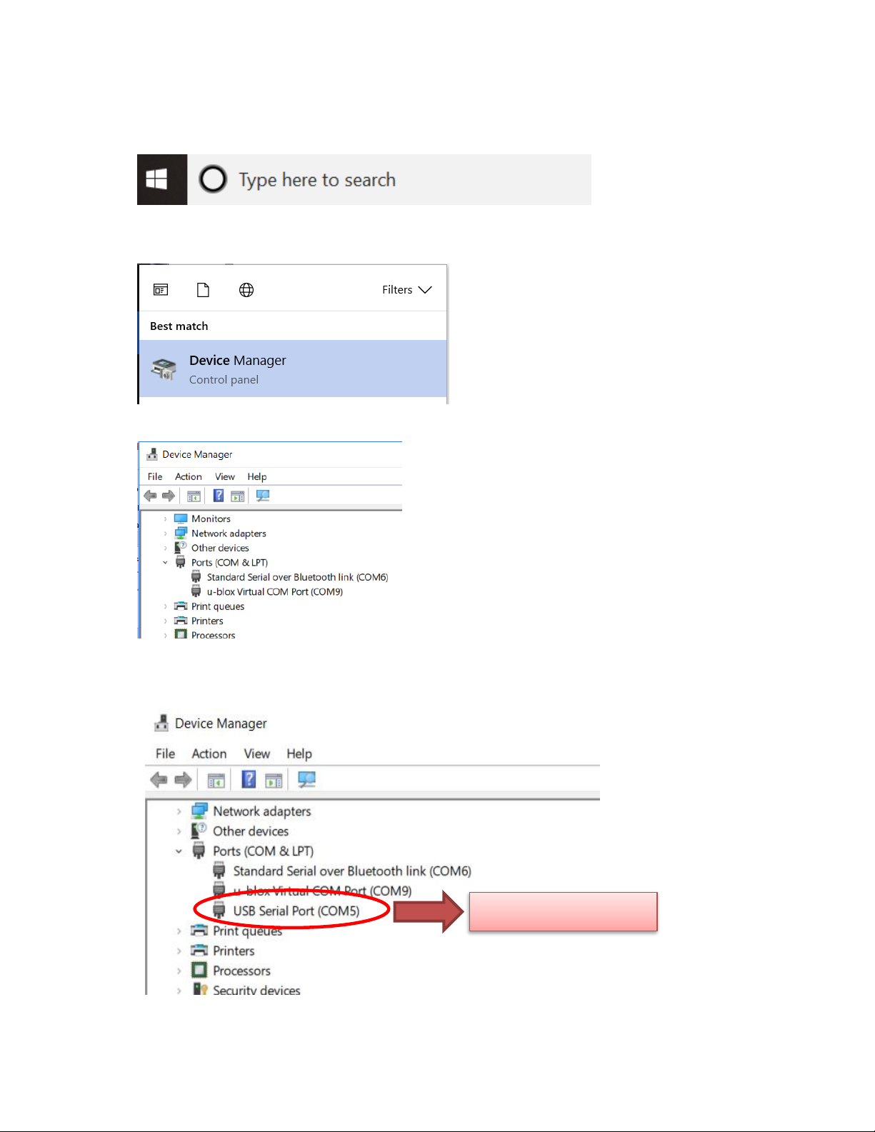
To find and launch device manager, put “device manager” in windows search.

.
Launch device manager.

Device manager appears as shown below before plug in USB/charge cable to Atom.

Plug in USB/charge cable to Atom and new comport for Atom appears.

Comport is 5

72

02/06/2019, Rev. 1.6

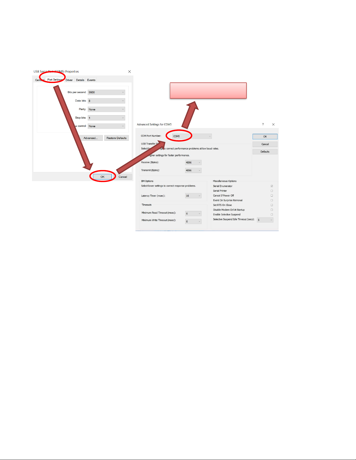
If comport number is not shown in the device manager, right click the comport for Atom and show

“Properties”.

Comport is 5

73

02/06/2019, Rev. 1.6

C3) Show Atom AU status by SPACPlus

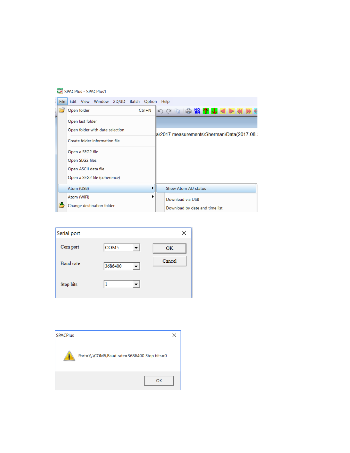
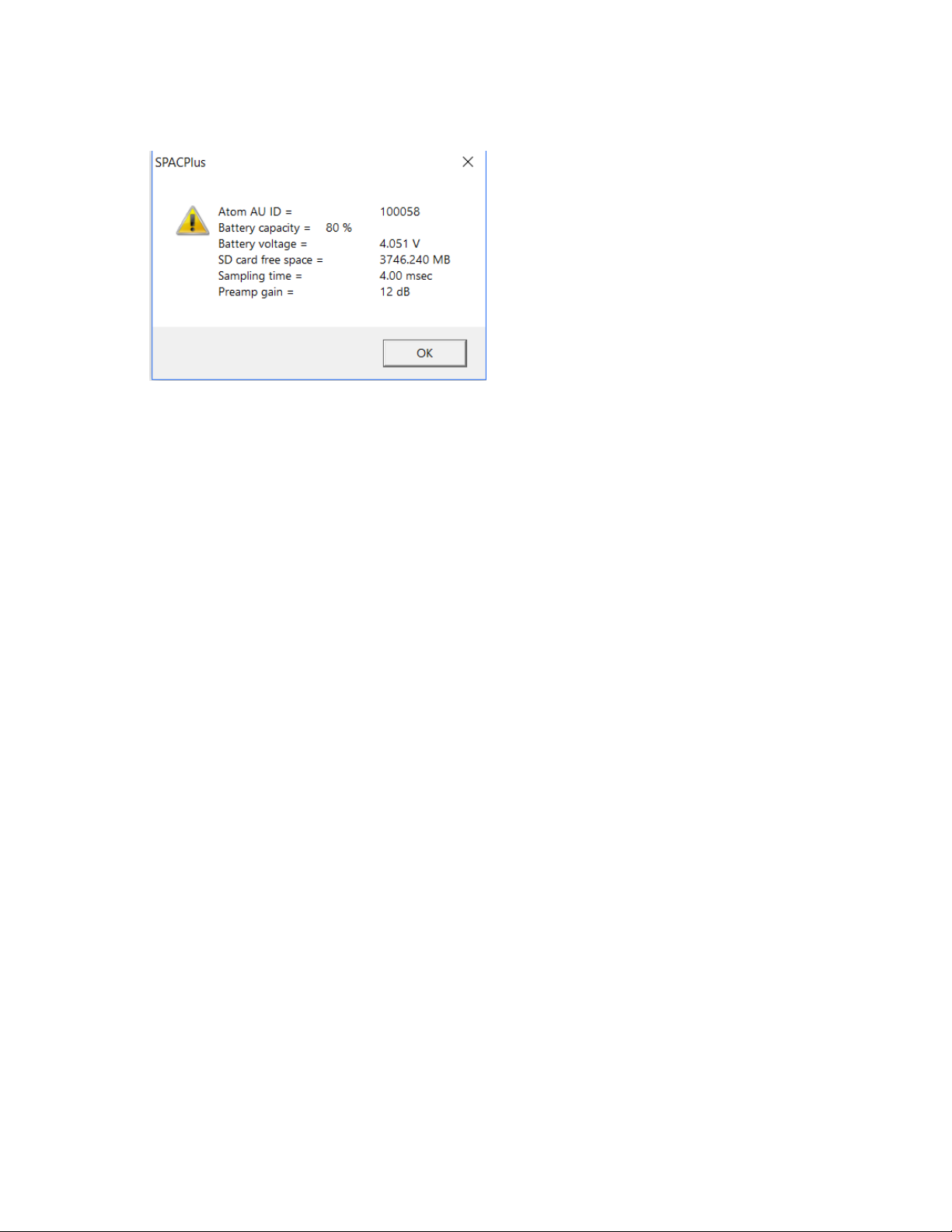
It is better to show the Atom AU status to confirm the connection and status of Atom unit before

downloading data. Launch SPACPlus and select [File]>>[Atom (USB)]>>[Atom AU status”] to show Atom SU

status.

Select comport and set baud rate to 3686400.

Message shown below implies that the comport was successfully opened.

Click “OK” and Atom AU status appears.

74

02/06/2019, Rev. 1.6

75

02/06/2019, Rev. 1.6

C4) Download data from Atom AU
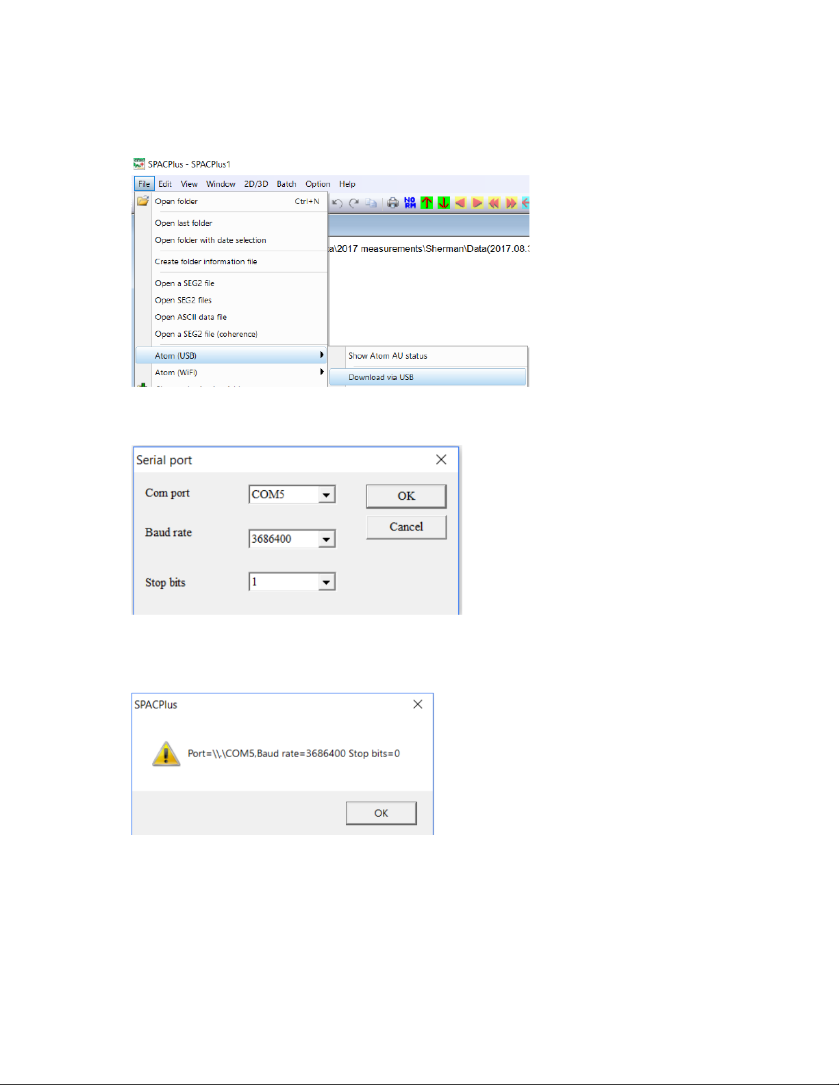
Select [File]>>[Atom (USB)]>>[Download via USB] to download data.

Select comport and set baud rate to 3686400.

Message shown below implies that the comport was successfully opened.

76

02/06/2019, Rev. 1.6

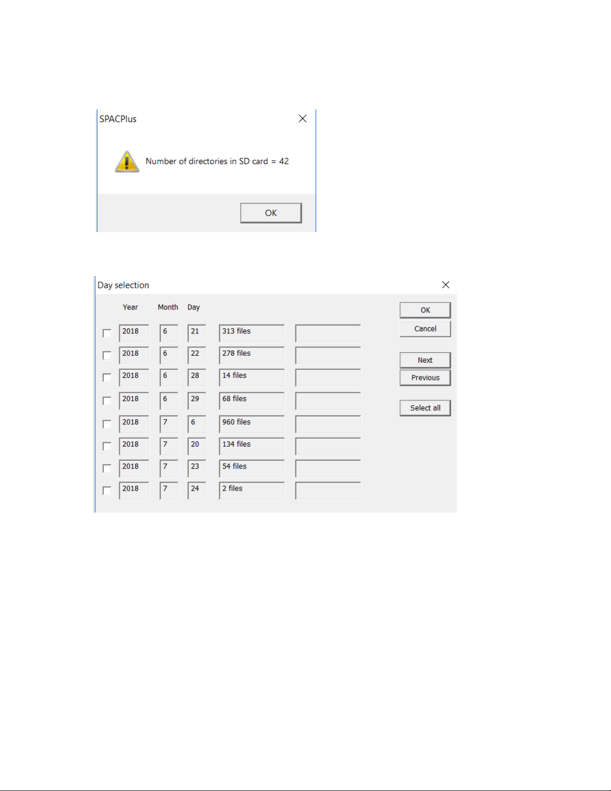
Number of directories appears.

Selection of data is the same as Wi-Fi.

Figure C.1 Selection of data to be downloaded.