

Page 1

Functional MRI User's Guide
Michael A. Yassa
● The Division of Psychiatric Neuroimaging ●
● Department of Psychiatry and Behavioral Sciences ●
●
The Johns Hopkins School of Medicine ●
● Baltimore, MD ●
1
Page 2

Document written in OpenOffice.org Writer 2.0 by Sun Microsystems
Publication date: June 2005 (1st edition)
Online versions available at http://pni.med.jhu.edu/intranet /fmriguide/
Acknowledgments:
This document relies heavily on expertise and advice from the following individuals
and/or groups: John Ashburner, Karl Friston, and Will Penny (FIL-UCL: London), Kalina
Christoff (UBC: Canada), Matthew Brett (MRC-CBU: Cambridge), and Tom Nichols
(SPH-UMichigan, Ann Arbor). Some portions of this document are adapted or copied
verbatim from other sources, and are referenced as such.
Supplemental Reading:
Frackowiak RS, Friston K, Frith C, Dolan RJ, Price CJ, Zeki S, Ashburner J, & Perchey G
(2004). Human Brain Function, 2
nd
edition, Elsevier Academic Press, San Diego, CA.
Huettel SA, Song AW, McCarthy, G. (2004) Functional Magnetic Resonance Imaging.
Sinaur Associates, Sunderland, MA.
2
Page 3

Table of Contents
Magnetic Resonance Physics..............................................................................6
How the MR Signal is Generated.............................................................................6
The BOLD Contrast Mechanism..............................................................................8
Hemodynamic Modeling.........................................................................................10
Signal and Noise in fMRI........................................................................................12
Thermal Noise.......................................................................................................12
Cardiac and respiratory artifacts............................................................................12
N/2 Ghost..............................................................................................................12
Subject motion.......................................................................................................12
Draining veins........................................................................................................13
Scanner drift..........................................................................................................13
Susceptibility artifacts............................................................................................13
Experimental Design...........................................................................................14
Cognitive subtractions ...........................................................................................14
Cognitive Conjunctions...........................................................................................14
Parametric Designs................................................................................................14
Multi-factorial Designs............................................................................................15
Optimizing fMRI Studies.........................................................................................15
Signal Processing..................................................................................................15
Confounding Factors.............................................................................................15
Control task............................................................................................................16
Latent (hidden) factor.............................................................................................16
Randomization and Counterbalancing...................................................................16
Nonlinear Hemodynamic Effects............................................................................16
Epoch (Blocked) and Event-Related Designs .......................................................17
Spatial and Temporal Pre-Processing...............................................................18
Overview................................................................................................................18
Raw Data ...............................................................................................................18
Getting Started.......................................................................................................18
Requirements.........................................................................................................19
Hardware Requirements........................................................................................19
Software Requirements.........................................................................................19
Software Set-up......................................................................................................19
The SPM Environment...........................................................................................20
Data Transfer from Godzilla...................................................................................20
Volume Separation and Analyze headers .............................................................21
Buffer Removal.......................................................................................................24
Slice Timing Correction (For event-related data)...................................................24
To Correct or Not to Correct..................................................................................24
Philips Slice Acquisition Order...............................................................................25
Which Slice to Use as a Reference Slice...............................................................25
Timing Parameters.................................................................................................26
Rigid-Body Registration (Correction for Head Motion)...........................................26
3
Page 4

Creating a Mean Image.........................................................................................26
Realignment...........................................................................................................27
Anatomical Co-registration (Optional)....................................................................29
Co-registering Whole Brain Volumes.....................................................................30
Co-registering Partial Brain Volumes.....................................................................30
Spatial Normalization to Standard Space..............................................................30
Correcting Scan Orientation..................................................................................31
Normalization Defaults...........................................................................................31
Normalization to a Standard EPI Template............................................................32
Gaussian Smoothing.............................................................................................33
Summary of Pre-processing Steps........................................................................34
Statistical Analysis using the General Linear Model.......................................35
Modeling and Inference in SPM.............................................................................35
Model Specification and the SPM Design Matrix ..................................................35
Setting Up fMRI Defaults.......................................................................................36
Model Specification................................................................................................36
Estimating a Specified Model................................................................................39
Global Intensity Normalization................................................................................40
Temporal Filtering...................................................................................................40
Results and Statistical Inference............................................................................42
Contrast Specification............................................................................................42
Thresholding and Inference ..................................................................................43
Rejecting the Null Hypothesis.................................................................................43
Type I Error (Multiple Comparison Correction).......................................................44
Spatial Extent Threshold (Cluster analysis) ...........................................................46
Viewing Results using Maximum Intensity Projection ...........................................46
Small Volume Correction and Regional Hypotheses.............................................48
Extracting Results and Talairach Labeling.............................................................48
Time-Series Extraction and Local Eigenimage Analysis .......................................49
Plotting Responses and Parameter Estimates......................................................50
Anatomical Overlays..............................................................................................53
Editing, Printing and Exporting SPM output...........................................................55
Region of Interest (ROI) Analyses......................................................................56
Anatomical vs. Functional ROIs ............................................................................56
MarsBaR (MARSeille Boîte À Région d'Intérêt) ....................................................57
Overview of the Toolbox........................................................................................57
ROI Definition........................................................................................................57
Running an ROI Analysis ......................................................................................59
Group-Level Analysis and Population-level Inferences...................................63
Inter-subject Analyses............................................................................................63
Fixed-Effects Analysis............................................................................................63
Random-Effects Analysis.......................................................................................64
Conjunction Analysis .............................................................................................66
Nonparametric Approaches....................................................................................67
False Discovery Rate.............................................................................................68
4
Page 5

Special Topics.....................................................................................................68
Cost Function Masking for Lesion fMRI.................................................................68
Advanced Spatial Normalization Methods.............................................................69
Using a Subject-Specific HRF in analysis .............................................................70
Guidelines for Presenting fMRI Data......................................................................73
5
Page 6
Magnetic Resonance Physics
How the MR Signal is Generated
The magnetic resonance (MR) signal arises from hydrogen nuclei, which are the only
dipoles abundant enough to be measured with reasonably high spatial resolution. The human
body is made up mostly of water (mainly hydrogen atoms). Hydrogen atoms possess a
magnetic property called spin which can be thought of as a small magnetic field. Spin is a
fundamental property of some nuclei (not all nuclei possess spin) and has two important
parameters: (1) size; spin comes in multiples of ½ and (2) charge; spin can be positive or
negative. Paired opposite-charged particles, e.g. protons and electrons can eliminate each
other's spin effects. An unpaired proton (e.g. in the case of hydrogen) has a spin of +½.
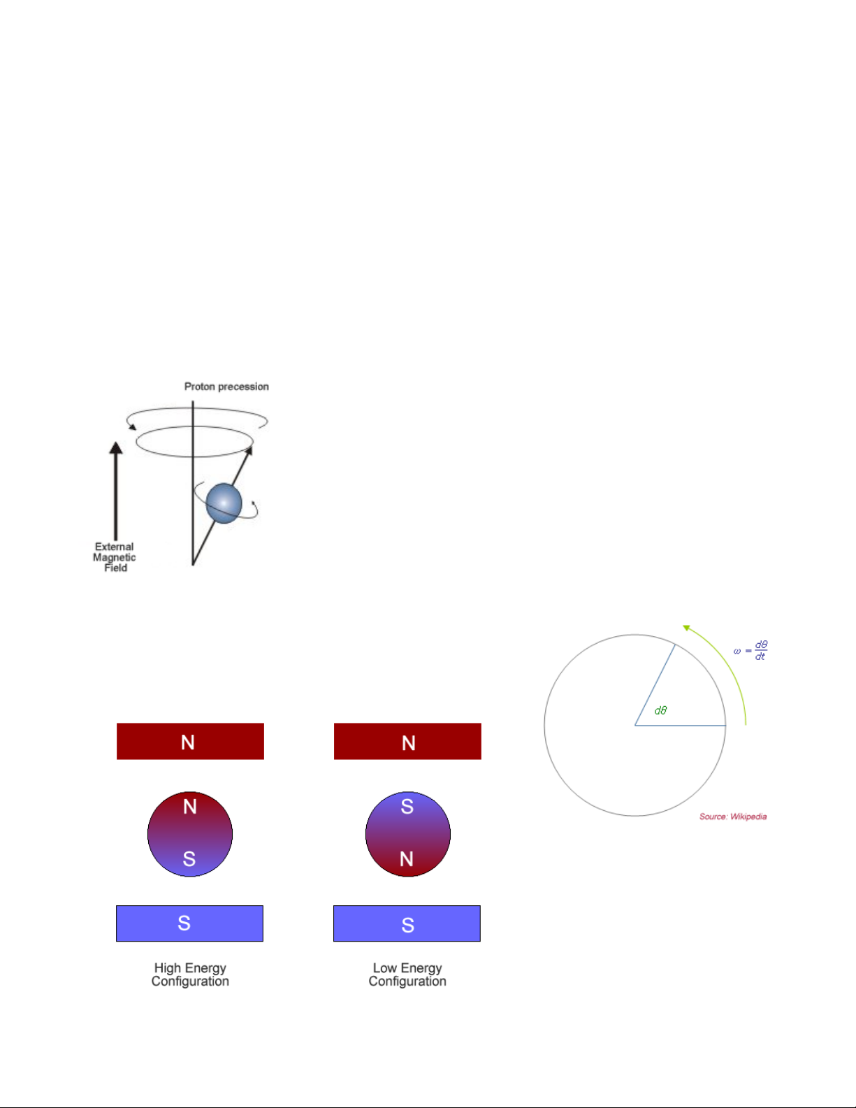
In an external magnetic field, a particle with non-zero spin will experience a torque which
aligns the particle with the field, by precessing (wobbling) around
the magnetic field axis (see figure on the left). The particle develops
an angular momentum, which is empirically related to its
gyromagnetic ratio (γ) (the ratio of the magnetic dipole moment to
the angular momentum of the particle). This value is unique to the
nucleus of each element (For Hydrogen, γ = 42.58 MHz/T). The
value's derivation is too complex to explain here. Instead we will
describe its relationship to the precession angular frequency (ω)
of a proton. Angular frequency is a scalar measure of how fast a
particle is rotating around an axis (see figure on the right)
ω
Larmor
The above is known as the Larmor Equation named
after Joseph Larmor, an Irish physicist (1857-1942). It
describes the relationship between the angular frequency (ω)
of precession and the strength of the magnetic field B. There
= γ Β
are two possible configurations for
proton alignment; one configuration
possesses higher energy than the
other (see figure on the left). A
proton can undergo a transition
between the two energy states by
absorbing a photon that has
enough energy to match the energy
6
Page 7
difference between the two states. This energy E is related to the photon's frequency ν by
Planck's constant h (6.626 x 10
-34
J-sec)
E = h ν
This frequency is associated with a spin flip and is often used to describe the Larmor frequency
as well.
Larmor
= ν
ω
In the context of MRI, a radio-frequency (RF) pulse is applied perpendicular to the static
magnetic field (B
). This pulse, which has a frequency equal to the Larmor frequency, shifts
0
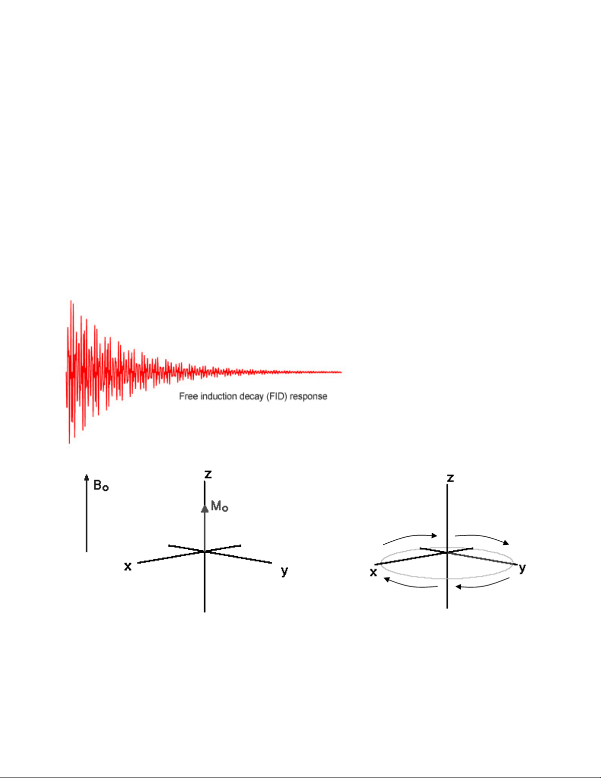
protons into a higher energy state. When the RF pulse (BRF) stops, the protons return to
equilibrium such that their magnetic moment is parallel again to B0. During this process of
nuclear relaxation, the nuclei lose energy by emitting their own RF signal. This is referred to as
a free-induction decay (FID) response signal. The FID response signal is measured by a field
RF coil, and has the characteristic shape shown in the figure below.
The Rf coil measure the relaxation
of the dipoles in two dimensions. The
Time-1 (T1) constant measures the
time for the longitudinal relaxation in
the direction of the B0 field (shown
below on the left). It is referred to as
spin-lattice relaxation.
The Time-2 (T2) constant
measures the time it takes for the
transverse relaxation of the dipole in
the plane perpendicular to the B0 field
(shown below on the right). It is
referred to as spin-spin relaxation.
The T
combined time constant (in physiological tissue) is called T
relaxation process is affected by molecular interactions and variations in B0. The
2
* (T2 star). In the case of MRI, we
2
take advantage of the fact that physiological tissue does not contain not a homogeneous
magnetic field, and thus the transverse relaxation is much faster. The size of these
inhomogeneities depends on physiological processes, such as the composition of the local
blood supply.
7
Page 8
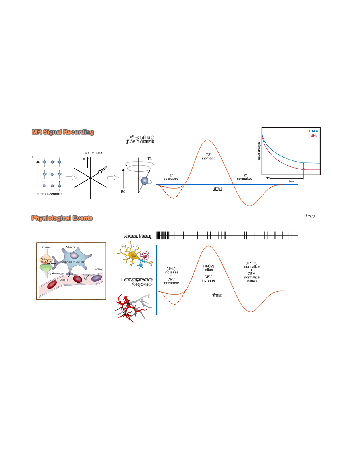
The BOLD Contrast Mechanism
This mechanism is employed in most fMRI studies. The idea is that neural activity
changes the relative concentration of oxygenated and deoxygenated hemoglobin in the local
blood supply. Deoxyhemoglobin (dHb) is paramagnetic (changes the MR signal), while
oxyhemoglobin is diamagnetic (does not change the MRI signal). An increase in dHb causes the
T2* constant to decrease. This was first noticed by Ogawa et al. In 1990 1 in the rodent brain,
and over the following few years became the mainstay of functional MRI. The BOLD Contrast
refers to the difference in T2* signal between oxygenated (HbO2) and dexoygenated (dHB)
hemoglobin.
The above figure illustrates the physiological events that underlie our recording of the MR
signal. Upon stimulation, neural activation occurs, which pulls oxygen from the local blood
supply. Theoretically, as the paramagnetic dHb increases, the field inhomogeneities are
enhanced and the BOLD signal is reduced. However, the dHb increase is tightly coupled with a
surge in cerebral blood flow (CBF) which compensates for the decrease in oxygen, delivering a
larger supply of oxygenated blood. The result is a net increase in cerebral blood volume (CBV)
and in Hb oxygenation, which decreases the susceptibility-related dephasing, increasing T2*
signal and in turn enhancing the BOLD contrast.
1 Ogawa S., Lee T.M., Nayak A.S., Glynn P. (1990). Oxygenation-sensitive contrast in magnetic resonance image
of rodent brain at high magnetic fields. Magn Reson Med 14:68-78.
8
Page 9
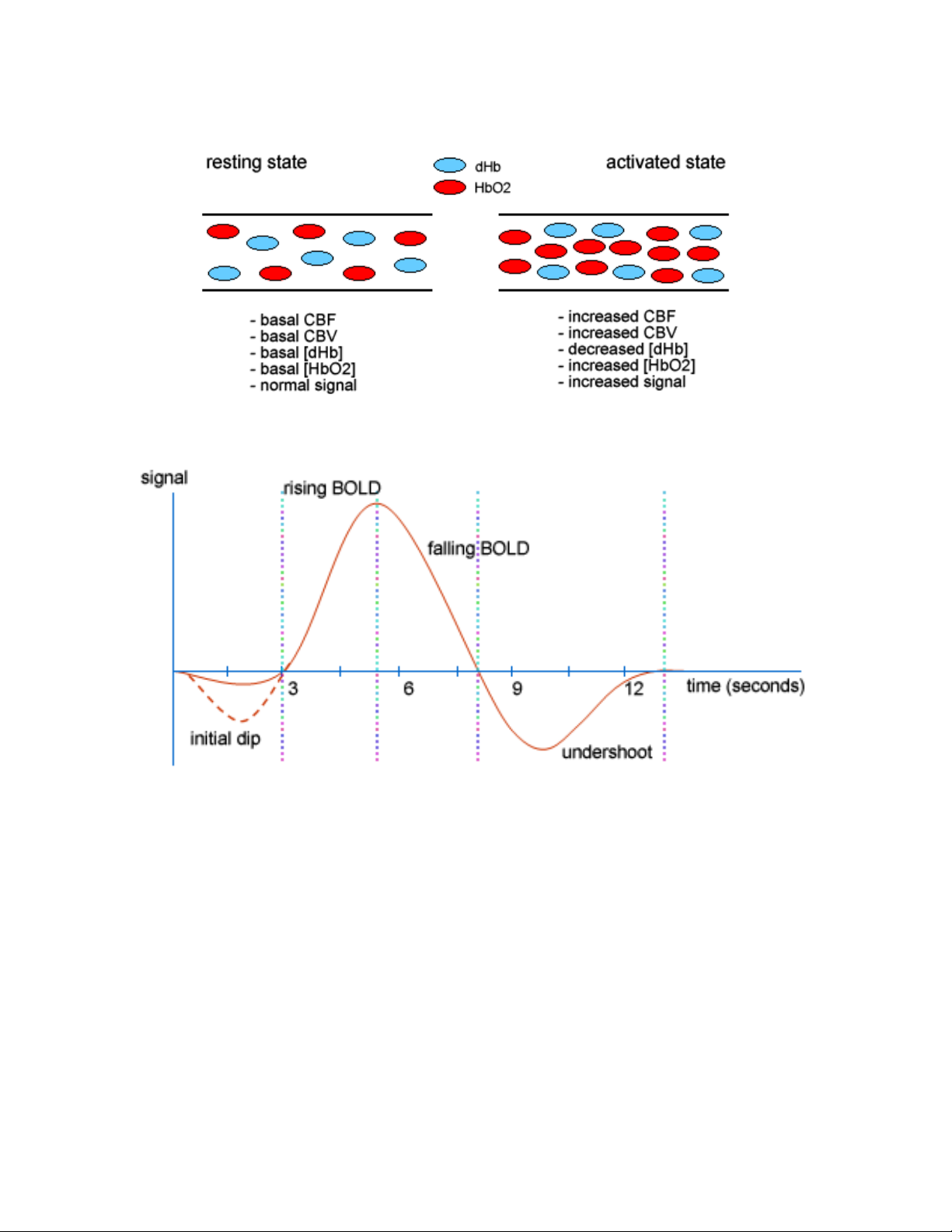
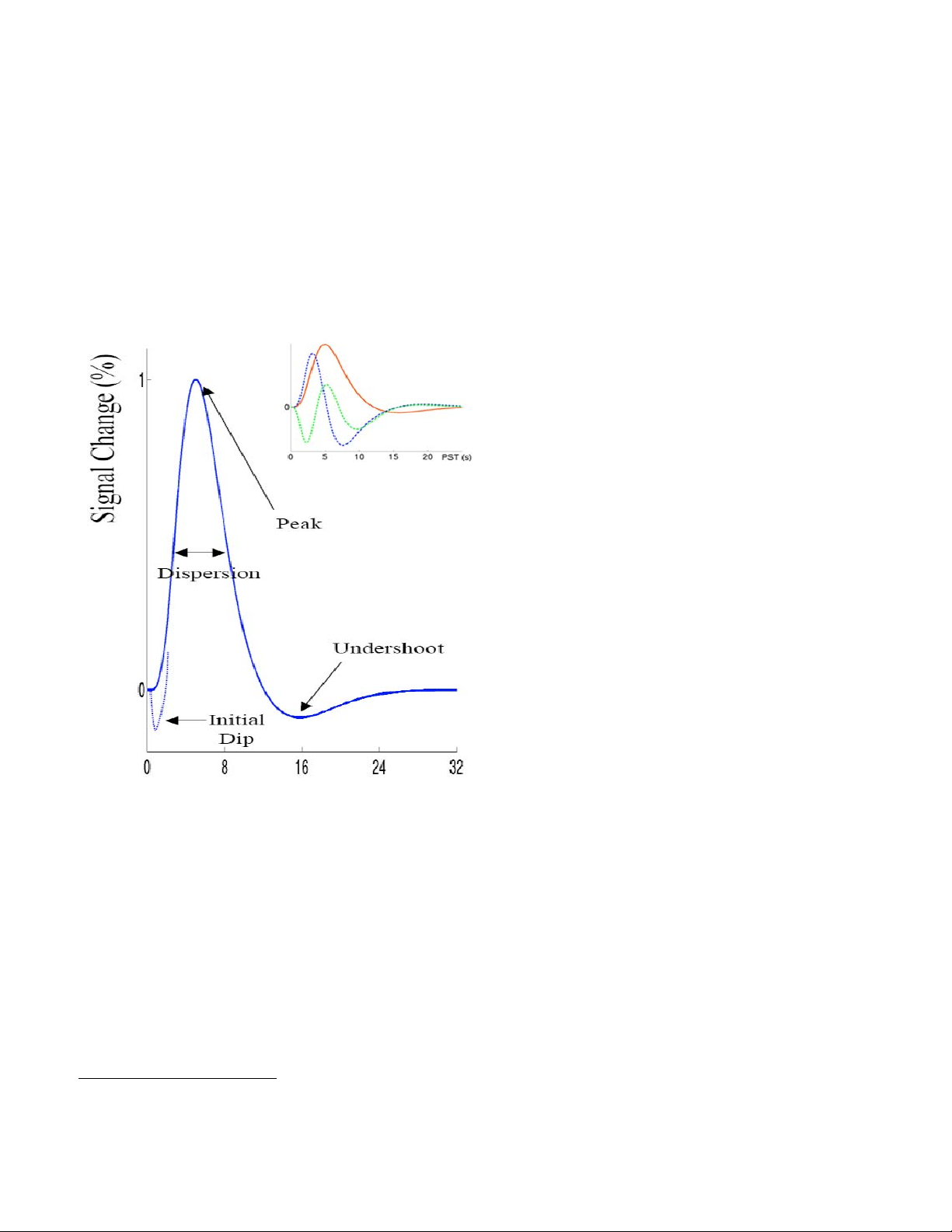
The BOLD response can be thought of as the combination of four processes:
(1) An initial decrease (dip) in signal caused by a combination of a negative metabolic and
non-metabolic BOLD effect. The local flow change as a result of the immediate oxygen
extraction leads to a negative metabolic BOLD effect, while the vasodilation leads to a
non-metabolic (or volumetric) negative BOLD effect.
(2) A sustained signal increase or positive BOLD effect due to the significantly increased
blood flow and the corresponding shift in the deoxy/oxy hemoglobin ratio. As the blood
oxygenation level increases, the signal continues to increase.
(3) A sustained signal decrease which is induced by the return to normal flow and normal
deoxy/oxy hemoglobin ratios.
(4) A post-stimulus undershoot caused by the slow recovery in cerebral blood volume.
9
Page 10

Hemodynamic Modeling
The BOLD response is very complex. The signal depends on the total of dHb, which
means that the total blood volume is also a factor. Another factor is the amount of oxygen
leaving the blood to enter the tissue (metabolic changes), which also changes the blood
oxygenation level. Finally, due to the elasticity of vascular tissue, increasing blood flow, changes
blood volume. All these factors have to be modeled adequately in order for us to estimate the
neural signal. The model currently employed in research and literature uses a canonical
hemodynamic response function that linearly transforms neural activity to the observed MR
signal. However, being able to get the true neural signal based on the hemodynamic counterpart
is a bigger problem.
Ideally, we would like to evaluate how well our linear transform model allows us to
estimate the actual neural signal. This can be done using simultaneous measurements of the
neural and BOLD signals.
Source: Logothetis and Wandell 2004
2
The above figure shows these simultaneous measurements in a monkey brain, using
extracellular field potential recording, together with fMRI. (a) the black trace is the mean
extracellular field potential (mEFP) signal; the red trace is the BOLD response. (b) spike activity
2 Logothetic NK, Wandell BA. (2004). Interpreting the BOLD signal. Ann Rev Physiol 66:735-69
10
Page 11
derived from the mEFP. (c) frequency band separation of the mEFP (d) estimated temporal
pulse response function relating the neurophysiological and BOLD measurements in monkeys.
Even though these recordings are problematic due to their invasive nature (cannot be done in
humans) and due to sampling bias, they provided useful evidence for the coupling of the neural
signal and the hemodynamic response.
In human fMRI, we can estimate the hemodynamic response function, using known tasks
with known and expected specific neural activation, e.g. visual, motor, etc... Results that are
consistent with what we already know about specific structures' involvement in cognitive
processes may provide some insight (even though it is at best speculative) into the neural
activation and the related hemodynamic
response. Over recent years, a more
descriptive canonical hemodynamic
response function has been developed that
accounts for the timing delay (temporal
derivative) as well as the duration (dispersion
derivative) of the response. This set of
functions is what SPM uses to estimate the
neural signal. The mathematics behind the
hemodynamic model are too complicated to
explain here, but more details are given in
the fMRI analysis section.
It is important to understand however that
this model is a 'best fit' model, which means
it does a good job of explaining variance in
the hemodynamic response after neural
stimulation. However, it does not explain all
the parameters. The metabolic and neural
processes that couple action potentials to
blood flow are still not well understood, and
are the subject of much of today's fMRI
research.
Animal research is attempting to carry out
more multi-modal experiments to produce empirical data to support or reject this model, and
human research is getting better at the deconvolution of the neural impulse using higher order
mathematical modeling.
From the above we can see the entire cycle takes about 30 seconds to complete. Early
event-related studies were limited by this, and thus had to use very long inter-stimulus intervals
to allow the response to return to baseline before another one started. If the hemodynamic
responses were perfectly linear, then they should not have been hindered by this, as the linear
summation of HRFs can be deconvolved easily. However, BOLD response non-linearities exist,
and pose a problem. This non-linearity can be thought of as a “saturation” effect where the
response to a series of events is smaller than would be predicted by the sum of the BOLD
3
responses from the individual events. Empirically, it has been found that for SOA
of below ~8
seconds, the degree of saturation increases as the SOA decreases. However, for SOA of 2-4
3 SOA: Stimulus Onset Asynchrony – This is the amount of delay between the presentation of one experimental
stimulus to another.
11
Page 12
seconds, the magnitude of saturation is small. This is important to think about in designing an
fMRI experiment, and is particularly of importance in discussing rapid event-related fMRI.
To summarize, the general shape of the hemodynamic response is the same across
individuals and cortical areas. However, the precise shape varies from individual to individual
and from area to area. Canonical modeling however offers us a powerful tool to be able to
reasonably estimate the neural signal, based on the observed changes in regional cerebral
blood flow.
Signal and Noise in fMRI
The magnitude of the BOLD response signal we are trying to measure in fMRI is very
small compared to the overall MR signal. We can improve our signal detection ability by
increasing the amplitude of the signal or reducing the amplitude of the noise. The type of control
is referred to as signal-to-noise ratio or SNR. There are many different sources of noise that
produce artifacts in the scanner. Here is a brief description of some of the most common
problems:
Thermal Noise
Thermal noise is produced due to the thermal motion of electrons
inside the subject's body and in the large electronic circuits of the MRI
scanner. This type of intrinsic scanner noise is uncorrelated to the task
and the hemodynamic signal, and therefore can be described as “white”
noise. This type of noise increases with increased resolution (smaller
voxels). Therefore controlling it is a trade-off with the resolution of the
images.
Cardiac and respiratory artifacts
The pulsation of the blood and changes connected to breathing can change blood flow
and oxygenation. These factors create high frequency signal artifacts, for example, the cardiac
cycle is too fast (500 ms) to be sampled with a relatively average TR (2000 ms). However, when
this is the case, the variabilities become attributed to a lower frequency (aliasing), creating an
even larger problem.
N/2 Ghost
EPI scans in general suffer from ghosting artifacts in the phase
encoding direction. During acquisition, k-space data are sampled by an
alternating positive/negative read gradient. This results in a single ghost
shifted by half a FOV, known as the “Nyquist” or N/2 ghost. Using
readout gradient with the same polarity eliminates this problem at the
expense of lengthened data acquisitions.
Subject motion
Subject motion is the single most common source of series artifacts. Even relatively small
motion (of the range much smaller than a voxel size e.g 1.6-3.2 mm) can create serious artifacts
12
Page 13
due to the partial volume effects. Typically motion of about half a voxel in size will render the
data useless. Subjects should be instructed not to move, with their heads restrained securely.
The task design should also minimize the possibility of task related movements.
Draining veins
Large vessels draining in the brain could induce a hemodynamic signal, that may not be
easily differentiated from the hemodynamic responses related to the neural signal. This is hard
to control, thus caution should be taken in considering activation occurring close to visible large
vessels.
Scanner drift
Drift is created most probably by the small instability of scanner gradients. It can create
slow changes in voxel intensity over time. Even though the magnet contains huge
superconducting coils to maintain its magnetic field, the stability of this magnetic field is
occasionally drifts. This type of spatial distortion can also be caused by non-system factors, e.g.
the subject's head slowly moving downwards due to a possible leak in the vacuum pack holding
the head in place.
Susceptibility artifacts
The EPI images are very sensitive to the changes of the
magnetic susceptibility. In effect the signal from regions close to sinuses
and bottom of the brain may disappear. This can also be caused by the
presence of magnetic material in proximity of the gradients, e.g.
Implants, braces, buttons, or even another human body moving in the
room.
13
Page 14

Experimental Design
This section deals with the different designs that can be employed in neuroimaging
studies. Designs in general can be subdivided into categorical (or parametric) designs and multifactorial designs, with the latter being more complicated than the former.
Cognitive subtractions
These are one type of categorical design, which rely on the premise that the difference
between two tasks can be qualified as a separate cognitive components that is distinct in space
and therefore can be separated as an individual component of the hemodynamic response. An
example is a study in which visual and motor stimulation are combined in the experimental task
or condition, while the control task or condition consist of only the visual or only the motor
stimulation. Subtracting the activation in one condition from the other is expected to show only
the activation relevant to the specific type of stimulation. The problem with these designs is the
underlying assumption that the neural processes underlying behavior are additive in nature. Due
to the complexity of neural responses and the significant functional integration between various
brain structures, this assumption may not always hold true.
Cognitive Conjunctions
These designs can be thought of as a series of subtractions. Instead of testing a single
hypothesis pertaining to the activation in one task over the other, conjunctions test several
hypotheses at a time, asking whether all activations are jointly significant. For example, if we are
interested in verbal working memory, then we can use a series of tasks that have that cognitive
component in common, but nothing else in common. The conjunction of these tasks should
show only the structures that are involved in verbal working memory. Conjunction analyses
allow us to demonstrate neural responses independent of context.
Note: Testing joint significance using conjunctions is a notion that we will return to when we
discuss group fMRI analysis.
Parametric Designs
The underlying premise in these designs is that regional activation will vary systematically
with the degree of cognitive processing. For example, an fMRI study of hemodynamic
responses and performance on a cognitive task illustrates the utility of this design. Correlations
or neurometric functions may or may not be linear. Clinical neuroscience can use parametric
designs by looking for neuronal correlates of clinical ratings over subjects (e.g. symptom
severity, IQ, performance on QNE, etc..). The statistical design then can be viewed as a multiple
linear regression model. However, if one needed to investigate several clinical scores that are
correlated, we have a problem with running the regression model, since variables are not
orthogonal. In this case, factor analysis, or principal components analysis (PCA) is used to
reduce the number of possible explanatory variables, and render them orthogonal to each other.
14
Page 15
Multi-factorial Designs
These designs are more prevalent than single factor designs, because they offer more
information and allow us to investigate interesting interactions between variables, e.g. time by
condition interactions. For example pharmacological activation studies assess evoked
responses before and after the administration of a drug. Interaction terms would reflect the
pharmacological modulation of task-dependent activation. Interaction effects can be interpreted
as (a) the integration of cognitive processes or (b) the modulation of one cognitive process by
another.
Optimizing fMRI Studies
Signal Processing
An fMRI time series can be thought of as a mixture of signal and noise. Signal
corresponds to neurally mediated hemodynamic changes, while noise can be the result of many
contributions that include scanner artifacts, subject drift, motion, physiological changes (e.g.
breathing), in addition to neuronal noise (or signal mediated by neural activity that is not
modeled by explanatory variables). Noise in general can be classified as either white
(completely random), or colored (e.g. the pulsatile motion of the brain caused by cardiac cycles
and modulation of the static magnetic field by respiratory movement.
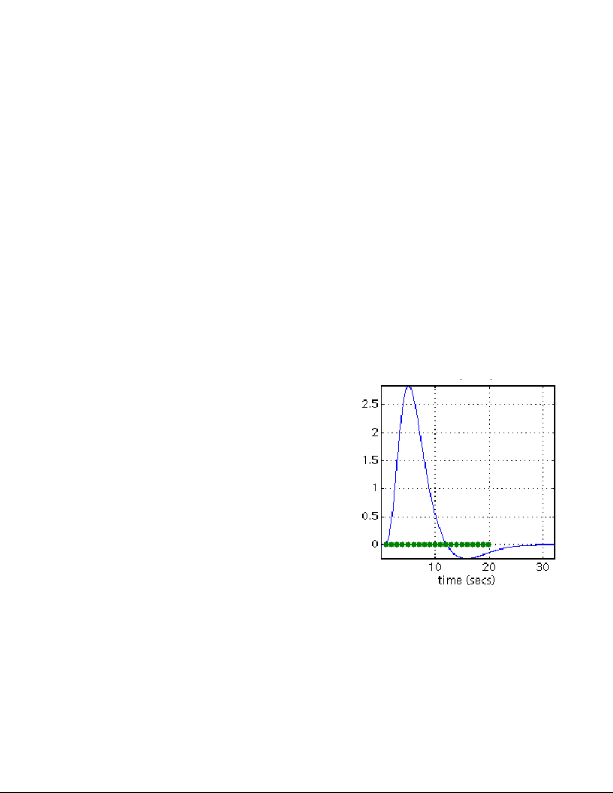
These effects are typically low-frequency or wideband. Thus in order to optimize an fMRI study, one
should place stimuli and the expected neural stimulation
in a narrow-band or higher frequency than the
physiological noise that is expected. This makes the
process of filtering and hemodynamic deconvolution
easier. For example, the dominant frequency of the
canonical HRF bandpass filter in SPM is ~0.03 Hz. In
order to maximize the signal passed by this filter, the
most efficient design would then be a sinusoidal
modulation of neural response with period ~32 s. In terms
of design, this means a blocked design using a box-car
function with 16s ON and 16 OFF epochs would be
optimal. The objective here is to comply with the natural
constraints of the hemodynamic response and ensure
that the experimental variance is detected in the
appropriate frequencies.
Confounding Factors
Any variable that co-varies with the independent variable is a confounding factor. These
can be due to variety of sources. For the most part, exerting experimental control on the task
can help resolve these issues. Optimized fMRI designs are generally more successful at
minimizing these factors.
15
Page 16

Control task
The control task is very important in a subtraction design. The idea is to make the control
condition very similar to the experimental condition, except for the variable we are trying to
assess. For example, in a study of face perception, one can use the control condition of simple
fixation. However, the two conditions would differ in more than one aspect, e.g. brightness,
edges, etc... If we use this design, we may not be able to make inferences about the activation
of interest, since it could have been solely due to the perception of a picture in general, and not
a face in particular. We can optimize this design by making the control task stimuli out of the
same faces, but transformed somehow, so that are no longer perceptible as faces, but rather as
images of noise (with a similar intensity histogram).
Latent (hidden) factor
This is one of the most dangerous confounding factors, and is due to the fact that
correlation does not imply causation. For example, you can give a group of Parkinson's disease
patients as well as a group of controls a motor activity task (repeated finger tapping) to
investigate activation in the motor cortex. You find that motor cortex activity is diminished in PD
patients compared to controls. This may lead one to conclude that PD patients under-activate
their motor cortex during motor movement. However, other explanations should also be
considered. In this case, it is possible that PD patients pressed the buttons less often, and
performed poorly on the task, which would explain the diminished activation. Here the latent
factor is performance, while our mis-interpretation of the data makes it seem like the diseased
state was really the causal factor.
Randomization and Counterbalancing
Trials and subjects should be sufficiently randomized, not to induce any confounding
effects. For example, if you test both patients and controls by day and night. You should
randomize whether night subjects are patients or controls. If you have two versions of the task
(or two conditions), you might want to randomize subjects to conditions, so that your subject-bycondition interaction is not a confounding factor. In the case where certain variables cannot be
adequately randomized, the investigator may choose to use a counterbalanced design. For
example if gender is randomly assigned to groups, it is possible that one group will have twice
as many men as the other. Counterbalancing ensures that this is not case, by balancing the
number of men and women in each group. Whether you randomize or counterbalance may
depend on your sample size (for example, in a small sample, randomization may not yield a
perfectly balanced design).
Nonlinear Hemodynamic Effects
This is manifested as a hemodynamic refractoriness or saturation effect at high stimulus
presentation rates. This means that the simple addition of hemodynamic responses is not
enough to deconvolve the individual events. This effect has an important implication for eventrelated fMRI, in which trials are usually presented in quick succession. This issue will be
addressed in detail in the following section.
16
Page 17

Epoch (Blocked) and Event-Related Designs
Typically, fMRI experimental design can be classified into two types: a blocked design
(epoch-related) and a single event design (event-related). Blocked designs are the more
traditional type and involve the presentation of stimuli as blocks containing many stimuli of the
same type. For example, one may use a blocked design for a sustained attention task, where
the subject is instructed to press the button every time he or she sees an X on the screen.
Typically blocks of stimulation are separated from each other by equivalent blocks of rest (where
the subject may be instructed to passively attend to a fixation cross on the screen. This type of
design is depicted below.
Blocked designs are simple to design and implement. They also have the added
advantage that we can present a large number of stimuli, and thus increase our signal to noise
ratio. It has excellent detection power, but is insensitive to the shape of the hemodynamic
response. We also have to assume a single mode of activity at a constant level during
stimulation. In other words, we cannot infer any information regarding the individual events. This
precludes us from being able to investigate interesting questions, such as the relationship of
activation to accuracy and performance or reaction time. We use blocked designs if we plan to
use a cognitive subtraction or conjunction to analyze our data.
The alternative to epoch designs is a more powerful estimation method. Event-related
fMRI has emerged as a much more informative method that allows for a number of other
analyses to be conducted. Rapid, randomized, event-related fMRI is the newest improvement
on this concept. The idea is to present individual stimuli of various condition types in randomized
order, with variable stimulus onset asynchrony (SOA). This provides us with enough information
for time-series deconvolution using a canonical or individual-derived HRF, and allows us to
conduct post-hoc analyses with trial sorting (accuracy, performance, etc...). This design is more
efficient, because the built-in randomization (jittering) ensures that preparatory or anticipatory
effects (which are common in blocks designs) do not confound event-related responses. A
typical event-related design is depicted below.
Mixed designs are also possible (combining aspects of blocked and event-related
designs, however they are much more complicated to design and analyze. They usually contain
blocks of control and experimental stimuli, however within each block are multiple types of
stimuli. It allows us to simultaneously examine state-related processes (best evaluated using a
block design) and item-related processes (best evaluated using an event-related design).
17
Page 18

Spatial and Temporal Pre-Processing
Overview
Functional MRI (fMRI) pre-processing is designed to accomplish several purposes. It
corrects for head motion artifacts during the scan (realignment), adjusts the data to a standard
anatomical template (normalization) and convolves the data with a smooth function suitable for
analysis (smoothing). The pre-processing is done within the Statistical Parametric Mapping
(SPM) environment which is a MATLAB package with a graphical user interface (GUI).
Additional MATLAB functions will be used and will be described in detail. Depending on the
computer speed and dataset size, pre-processing can take several hours or days.
Pre-processing also requires a lot of hard drive space, for example if a single subject’s
dataset is 1000 MB (1GB) in size, you will need 5000 MB (5GB) of space to pre-process the
subject’s data. Of course once the pre-processing is done, a lot of the data generated in the
intermediate steps can be deleted, and this can be used to save hard drive space. The preprocessing directory should be either (1) an internal drive at 7200 RPM or more (RAID-0 SATA
or 10-15K SCSI preferred) or (2) an external drive at high throughput rates. FireWire is the
recommended medium, due to its reliability and high throughput rates (800 Mbps on machines
that support 1394b). Pre-processing, in general should not be done over the network (i.e. writing
images to a mapped network drive), as it takes longer, and makes the process more prone to
crashing (this is severely affected by network traffic). However, you may run pre-processing on
another computer on the network, using remote desktop (and the pre-processing computer's
native Matlab/SPM). For instructions on how to set up the remote desktop, please see
http://www.microsoft.com/windowsxp/using/mobility/default.mspx
Raw Data
fMRI datasets are saved at the point of origin (Philips scanner) as combinations of
.par/rec files. This data is saved on Godzilla (large capacity UNIX-based server, maintained by
the F.M. Kirby Research Center: for questions about Godzilla or to set up a user account,
please contact its administrator, Joe Gillen (jgillen@jhu.edu
combination of the subject’s last name and the reverse date of the scan, followed by the scan
number (scans are numbered in the same order in which they were acquired), e.g.
“yassa050103_3.rec”. You may let the technicians know to save the files using a different name
(HIPAA regulations somewhat preclude saving these files with the subject last name).
). Data is usually saved as a
Getting Started
To start a new analysis on your computer, first you must create a new working directory
for storing all of the data files in your dataset. You have to make sure the drive on which you
save the data has enough space to contain all the images. Then you should create a directory
(without spaces in the directory name), e.g. “C:\fmri\subjID\” to contain all of the subject’s fMRI
data. It is a good idea to keep your imaging data organized by project and by subject. fMRI data
involves potentially thousands of files and thousands of data points, so it is essential to keep
everything organized and document this organizational structure somewhere safe.
18
Page 19

Requirements
Hardware Requirements
You must have the following hardware requirements before you begin:
- Windows XP Professional or Windows 2000 or Redhat Linux 9.0 and above.
- At least 20 GB of free space (60 recommended)
- At least 1 GB of RAM (2 – 4 GB recommended)
- 4 GB of swap space (also known as paging file on Windows)
- Dual processors recommended.
Software Requirements
You must have the following software on your computer, before you begin:
- Matlab 6.0 or higher with SPM99 and its latest updates (download)
- Secure Shell SSH Software
If you do not have any of these requirements, you should contact Arnold Bakker or Mike Yassa
to make sure you have the correct setup.
Software Set-up
Install Matlab 6.1 (or above) in its default directory. If you’re using a network installation
of Matlab, you may need to be on an enabled Matlab client (we have a limited number of client
licenses). We also have a personal licensed version of Matlab which is more convenient and
can be installed without the need for network setup.
Download SPM99 from http://www.fil.ion.ucl.ac.uk/spm/ and extract it in a suitable
directory, e.g. “C:\spm99” or “C:\Matlab6p1\spm99”. Find the file “r2a.m” under
\\Soma\Matlab_functions . If you do not have access to Soma, contact Mike Yassa or Arnold
Bakker to get a copy of r2a. Copy and paste the file in your SPM99 directory.
Open Matlab 6.1 and add SPM99’s directory to the Matlab path, by going to File> Set
Path, and adding the SPM99 folder. Save the appended path, and close the “Set path“ window.
To check that everything has been installed correctly, type “spm fmri” in the Matlab console and
wait for the SPM windows to pop up. If you get error messages at this point, then your
installation was unsuccessful or your options are not set correctly.
Note regarding SPM use: SPM is a very resource-hungry program that can be very
temperamental. Make sure you close other open windows and other “memory hogging”
programs, before you start pre-processing or analyzing using SPM. At times it may also
spontaneously suffer from an internal error and indicate this by printing a verbose and cryptic
output to the Matlab command window. It may also crash or lock up your Windows system
entirely. If this happens, then shut down SPM and restart Matlab (restarting Matlab clears its
cache memory, and is necessary before you start the same process again).
19
Page 20
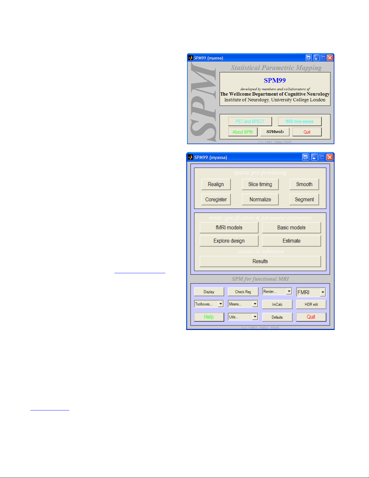
The SPM Environment
Statistical Parametric Mapping (SPM)
main panel allows you to select between two
interfaces, one for fMRI and one for
PET/SPECT modeling. In order to bring up this
screen, type >spm at the Matlab console. Click
on <fMRI Time-series> to bring up the fMRI
interface. If you are running spm2 as well, make
sure that the spm99 directory is prepended to
the top of the Matlab path. Matlab will run
whichever instance of spm it finds in its path
first.
Three SPM windows should appear. The
Upper window will be referred to as the fMRI
switchboard. The lower left window is the SPM
input window, and the right window is the SPM
graphics output window. The switchboard
consists of a spatial preprocessing panel with
option for processing fMRI data. The statistical
analysis panel containing the different linear
models that can be applied to the data. And
finally, the bottom panel contains useful tools for
displaying images, changing directories,
creating means, changing defaults, writing
headers, and running different toolbox options.
Toolboxes are installed in \\spm99\toolbox. The
<Defaults> button changes the defaults only for
the current session. If you close and restart
SPM or Matlab, those changes will be lost. You
can make permanent changes to fMRI defaults
by editing the spm_defaults.m file (or creating
an alternate version for your lab, and placing it
in the Matlab path before the spm directory.
Data Transfer from Godzilla
Godzilla is a large RAID array, acting as a storage server at the F.M. Kirby Research
Center at Kennedy Krieger Institute. It is the default image repository. We use this server to
transfer subject data from the scanner to our laboratory. Once a subject's data is acquired, it is
exported from the scanner database to a specific directory on Godzilla. Usually this is under one
of the two main disks (g1 or g2). Each investigator has a directory for storage and transfer, e.g.
\\g1\myassa
(godzilla.kennedykrieger.org) using your username and password. Once connected, in the top
menu bar go to <Operation> and Select <Go to Folder>. In the folder window enter the folder
. Open Secure Shell (SSH) File Transfer Window, and connect to Godzilla
20
Page 21
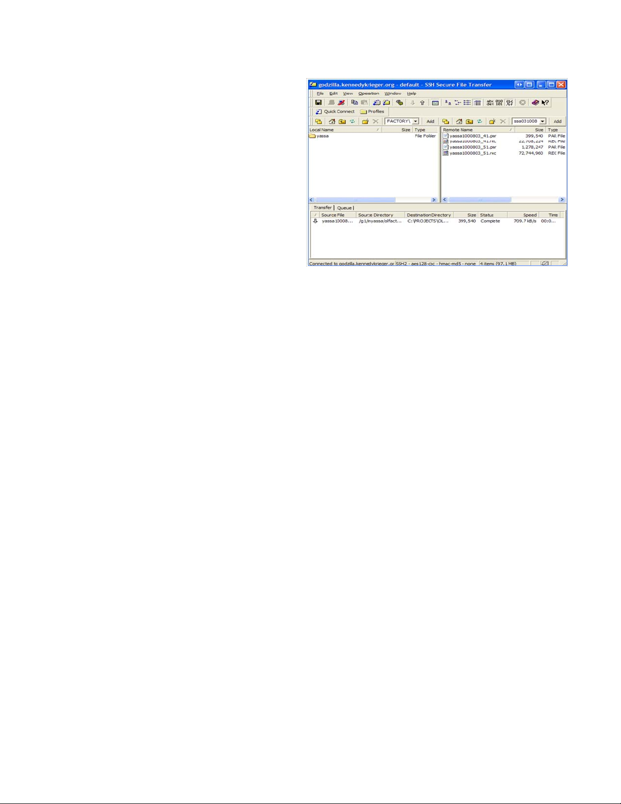
name e.g. “/g1/studyPI” and press <Enter>.
This is shown on the left.
In the left window, change the
local folder to the data folder you set up for the
study/ subject. In the right window, navigate
through the remote directories and find the
subject whose data you would like to preprocess. Click and drag the directory with the
correct subject name/date to your local folder.
The individual files will be queued for transfer
sequentially. This process takes quite a bit of
time, and depends on network speed and
traffic. Wait for the transfer to be completed
before you close Secure Shell SSH.
Volume Separation and Analyze headers
This step involves the conversion of the Philips REC/PAR file format to the conventional
3D Analyze format (SPM can only handle Analyze images). The REC file contains all of the time
series images, and the PAR file is the text file containing all the parameters necessary to
separate the REC file into Analyze volumes. Rename the directories and par/rec combinations
to names that identify the subject ID and the session number, e.g. replace
“lastname051112_10_1.par” with “50100_4.par” where “50100” is the subject ID and “4” is the
session number. One way to separate the volumes uses the executable file “separate.exe”
which can be copied from \\Soma\Software\. If you do not have access to Soma, contact Mike
Yassa or Arnold Bakker to get a copy of the file. Separate uses a command line (DOS-like)
interface and requires you to know and/or calculate some of the parameters of your scan
acquisition. First you need to open your .par file. Right click the .par file and select “Open
With…”. Select Wordpad from the list of programs. The header file should look like this:
. Patient name : Yassa,Michael
. Examination name : #-#/g1/myassa/yassa050131
. Protocol name : Bold396 SENSE
. Examination date/time : 2005.01.31 / 10:12:59
. Scan Duration [sec] : 798
. Max. number of slices/locations : 39
. Max. number of dynamics : 396
. Image pixel size [8 or 16 bits] : 16
. Scan resolution (x, y) : 80 80
. Scan percentage : 100
. Recon resolution (x, y) : 128 128
. Number of averages : 1
. Repetition time [msec] : 2000.00
. FOV (ap,fh,rl) [mm] : 230.00 117.00 230.00
. Slice thickness [mm] : 3.00
. Slice gap [mm] : 0.00
21
Page 22

The header file above has been truncated to only show the parameters of interest. The
Recon resolution is the reconstructed image matrix, and is what defines the image space. In the
case above, the matrix is 128 x 128 voxels (in the “x” and “y” planes). The plane of acquisition is
plane “z” and is determined by the Number of Slices
parameter, which in this case is 39. Thus
the image matrix is 128 x 128 x 39.
The Number of dynamics
parameter determines the number of functional scans or time
points in your series, for example 396 dynamics, means your rec file will be separated into 396
Analyze volumes.
The FOV (ap, fh, rl) parameter describes the field of view in three dimensions (“ap” is
anterior-posterior, “fh” is foot-head, and “rl” is right-left). Since the direction of acquisition of this
scan is axial (foot-head) that means the “fh” parameter (in this case, it is 117.00) is in the z
orientation.
The voxel dimensions
can be calculated from the image matrix and the field of view using
the following formula:
Voxel size = FOV (mm)
e.g. 230 x 230 x 117 = 1.8 x 1.8 x 3.0 mm
Matrix (voxels) 128 x 128 x 39 voxel
Once you locate the file “separate.exe” copy it to your “C:\Windows” or “C:\WINNT”
directory. Now click on Start>Run and type “cmd” to display the command prompt. Test that the
file is in the right location and works by typing “separate” at the console, then hitting enter. You
should get the following usage notification with a list of the arguments needed to separate
volumes.
Splits a set of volumes into individual files
Usage: separate <input_file_name> <output_filename> <head_bytes>
<volsize> <numvols> <bufsize> <avg value> <swap bytes? 0 or 1>
Here is an explanation of each of these arguments:
✗ <input_file_name> - this is the name of the .rec file you would like to separate. You have
to type the full location of the file e.g. “C:\my_fmri\scan1.rec”. Separate also does not like
spaces in folder or filenames.
✗ <output_file_name> - this is the root filename for the separated scans, for example
“scan1_sess1_”. Output files would be appended with the dynamic number, e.g.
scan1_sess1_0001.img etc…
✗ <head_bytes> - this is the number of bytes preceding the actual scan. Unless you have
specified this for your scan before acquisition, this parameter should be set to zero.
✗ <volsize> - this is the size of each volume in voxels, which is calculated from the
information retrieved from the header. This is the equivalent of the image matrix, e.g. 128
x 128 x 39. The product of those three numbers is the <volsize> parameter, which in this
case is 638976 voxels.
✗ <numvols> - this is the number of volumes in the dataset, which is also the number of
dynamics, e.g. 396. This is the number of volumes your dataset will be split into.
✗ <bufsize> - this is the number of blank “buffer” voxels you may add to the beginning and
end of each dynamic. We mostly do not use this parameter, but if you wanted to buffer
each dynamic with a two-dimensional slice you would enter a number equivalent to the
22
Page 23

product of your XY matrix, e.g. 128 x 128 which is 4096.
✗ <avg_value> - we do not use this parameter. Enter the number 0
✗ <swap_bytes> - each voxel is represented by two bytes of data and the swap parameter
specific which order in which those bytes are read in order to form a readable image.
Different operating systems read the bytes in different order. The scanner can be thought
of as a UNIX-based machine. Since we are operating on a Windows PC, we have to
swap the bytes to read the image. Enter the number 1.
Thus in order to separate the session 1 rec file in the example above, you would enter:
separate C:\fmri\50001_1.rec C:\fmri\50001_1_ 0 638976 396 0 0 1
There is no interactive output written to the screen. You will know when the process is
finished because the console will return to input mode with the flashing cursor.
You may want to browse through the directory where all the files have been made to
make sure that things went well. Is there the right number of files, (the "numvols" parameter)?
Are they all the same size? Are they all the correct size? If any of these things seems wrong,
check the original commands that you entered, check for inconsistencies, check for math errors
on your part and then try again.
In our example above, there should be 396 files of size 1.21 MB each in the directory
C:\fmri\50001 and they should be numbered sequentially from 50001_1_0000.img to
50001_1_0396.img. Note that you cannot double-click any of these files to view them, without
first writing Analyze headers for them (the next step). You may now close the command prompt
screen. The next steps will all be handled by SPM99.
Assuming Matlab and SPM99 are already installed and SPM99’s directory was appended
to the Matlab path, you may now create header (.hdr) files using SPM’s HDREdit facility.
Open Matlab and type “spm fmri” at the console. This should bring up the SPM windows.
At the fMRI switchboard window, click on <HDREdit>. The lower left box will contain a
series of options on a pull-down menu that asks you to set various values that describe the
images. Click on the drop down menu and select the first parameter:
Set Image Dimensions
: This is the same as the image matrix which you retrieved from
the .par file. Enter the matrix parameters separated by space, e.g. 128 128 39
Set Voxel Dimensions: This was also calculated using the formula, which in our example
yields 1.8 1.8 3.0 (Entered with spaces as separators again)
Set Scalefactor: Scalefactor is 1 unless otherwise specified.
Set Datatype: Datatype from the Philips scanner is 16-bit integer data. Byte swapping is
optional and depends on the dataset. Try selecting Int16 first. If after header specification and
displaying the images they look incorrect, then you probably need to select byte-swapped Int16.
Set Offset into file
: This is only specified if there is a buffer, otherwise it should be zero. (If
you do not set this option, it is set by default to zero).
Set Origin (x y z)
: This is the mathematical origin of the scan, and it by default set to 0 0
0. (If you do not set this option, it set by default to 0 0 0).
Set Image Description: Here you can type a text description of the images in the series,
e.g. subject ID, or a standard statement like “property of PNI”, etc… You may also leave this
field blank or choose not to set it.
Now select APPLY to images. The “SPMget” file selector window will be invoked. This is
23
Page 24

the standard way of selecting files in SPM. You can change the present directory from
C:\Matlab\work to the directory where your images are kept, and select all the *.img which you
wrote using the separate function. You will notice that SPM does not list all of the files, but
instead it abbreviates the files with similar names and uses only the common root while the
number of files sharing this root are marked with subscript numbers to the left of the name, e.g.
50001_1_*.img. In this case click on the filename root, and you should see that files 1-396
396
were selected (turns blue). You can select more than one file and more than one series to write
headers to. Once you have selected all the files for which you would like to write Analyze
headers, click Done. SPM will create header files for each image file you selected, using the
same filename as the image file, but using the extension .hdr instead. You will see the progress
in the bottom left window.
You can check that the headers were written correctly by double-clicking an image file,
and displaying it in MRIcro. If the images do not display correctly, it is possible that your
datatype should have been byte-swapped or that one or more of your parameters during
separation and/or header creation was incorrect.
Buffer Removal
In most fMRI acquisitions, the first few volumes acquired can be removed from the series
to be excluded from the analysis. This is done for two reasons. We have to make sure that the
net magnetization has reached steady state condition, and we also have to account for possible
hemodynamic effects that may be related to the start of the experiment, e.g. Scanner noise,
shifting stimulus, etc... If these scans are included in the analysis there will be a large change in
signal that is not related to experimental conditions per se, which should be avoided.
Before you remove any volumes, you have to make sure that these volumes were
acquired during rest (or fixation) and be sure that your model or design accounts for the lag that
will result in the timing parameters. If you would rather not use the first few scans as a buffer,
you can also use dummy scans to get magnetization to reach steady state before you start the
actual experiment. This can be specified in your MRI protocol on the Philips scanner. Check
with the MRI technician to make sure that enough dummy scans are included before the trigger.
Slice Timing Correction (For event-related data)
To Correct or Not to Correct
Functional MRI data from the Philips scanner are acquired slice-wise so that a small
amount of time elapses between the acquisition of consecutive (or in the Philips case interleaving) slices. Given a TR of 2000 ms, for example, in a 20-slice acquisition, each slice would
roughly take 100 ms to be acquired. This becomes an issue only in event-related designs where
one typically uses stimulus durations that elicit BOLD responses lasting only a couple of
seconds. For these designs it is critical that an appropriate temporal model is used, as any
difference between the expected and actual onset times may decrease the sensitivity of the
analysis. For short TR's (i.e. less than 3 seconds), slice timing correction can be used to remedy
this problem. Essentially this pre-processing step will determine the midpoint slice in the
acquisition and temporally interpolate all the other slices to this point.
Note: If slice timing correction is used, then one can use a naïve HRF model in the
analysis. If slice timing correction is not possible or is not performed, one can still model event-
24
Page 25

related data using HRF derivatives (more information on this in the analysis section).
Philips Slice Acquisition Order
In order to perform slice timing correction, click on the <Slice timing correction> button in
the SPM fMRI switchboard. Select all images in the series you would like to correct. Under
<Sequence type> select <user specified>. The Philips scanner acquires slices in an odd-evens
interleaved pattern (i.e. 1, 3, 5, 7, … 2, 4, 6, 8, …). In the empty box enter the correct slice order
from your acquisition. For example, if you acquire 20 slices, enter: 1 3 5 7 9 11 13 15 17 19 2 4
6 8 10 12 14 16 18 20 . Numbers should be separated by a single space, and all slices in the
acquisition should be included. Once you’re done click enter.
Note regarding slice acquisition order: At the point of scanning, you can specify and
let the MR technician know that you would like to acquire the scans in a sequential order (this is
the Kirby center default). If you do not change it, then they will be acquired according to the
Philips default (interleaved, odds then evens).
Which Slice to Use as a Reference Slice
The next prompt will be for the <Reference slice>. Enter the slice you want to consider as
a reference point. All other slices will be corrected to what they would have been if they were
acquired when the reference slice was acquired. The default is the middle slice (although,
please make sure the default value given is indeed the middle slice for the number of slices you
have).
The logic behind selecting the middle slice as a reference point for slice timing correction
is that this way there will be a minimum total shifting in time required, and therefore any
interpolation introduced by the correction procedure would be minimized. Some may argue that
in a perfect slice timing correction, the interpolation to any slice in the temporal sequence is the
same, and thus it doesn’t make any difference which slice you choose (even if it is in the space
outside the brain). However, SPM’s algorithm is not perfect and is worse for longer TR’s (more
10 as the reference slice.
Note: When the first slice in time is NOT used as a reference during correction, the default
sampled bin must be adjusted prior to analysis. More details in the analysis section.
25
Page 26

Timing Parameters
Once you’ve specified the reference slice, SPM will prompt you for <Repetition Time
(TR)>. This parameter is in your .par file, and is quite simply the amount of time it takes the
scanner to acquire a full volume. SPM will suggest a suitable TR by default, but this may not be
the correct TR. You must specify the correct TR for slice timing correction to work properly;
otherwise temporal artifacts may be induced.
Next, SPM will ask you to input <Acquisition time (TA)>, which is the time between the
beginning of acquisition of the first slice and the beginning of acquisition of the last slice of one
scan. Typically, this is calculated using the formula TA = (TR/#slices)*(#slices – 1). For
example, if TR = 2, #slices = 39, TA = 1.949. This default value is calculated by SPM for you,
and is displayed in the input box. You may accept this default value, but you may want to
confirm that it is indeed correct. This step will produce a* files, which are acquisition corrected. It
typically takes 20 minutes or so to correct a typical session (300 scans).
Rigid-Body Registration (Correction for Head Motion)
Image registration is very important in fMRI, since signal changes due to hemodynamic
responses can be masked by signal changes resulting from subject movement. Although, the
subject’s head is restrained as much as possible in the scanner, head motion cannot be
completely eliminated, thus retrospective motion correction (i.e. Realignment in SPM-speak) is
an essential pre-processing step. Image registration involves estimating a transformation matrix
that maps image A (the source image) onto image B (reference image (or target), which is
assumed to be stationary). A rigid-body transformation is defined by six parameters: 3
translations (x, y, z) and 3 rotations (x, y, z). This type of transformation is a subset of the more
general affine (linear) transformations.
Creating a Mean Image
Motion correction involves registering a source image to a target image. The target image
can be the first image in the series or it could be a mean image based on the entire series.
Since the subject could undergo some motion at the beginning of the scan session which
subsides as the scan goes on, it is better to calculate a mean image for the series and use this
image as the realignment target.
The output of the function spm_mean_ui.m is written to the current working directory, so
you should change this to your fmri directory before you create a mean. In the fMRI switchboard
click on the <Utils> drop down menu and select <CD> to change the current working directory.
Using the SPM folder selector window, navigate to the correct folder and select it. SPM should
display an alert with the new working directory name. Once this is done, you can click on the
<Means> drop down menu and select <Mean>. You will be prompted to select the images to be
averaged. Select all of your (slice timing corrected if event related) functional images. If you
have several sessions, you may want to select all images or a representative subset of images
from each session (MATLAB may crash if you try to average more than a few hundred images
at the same time). This process has no progress bar, but the output is printed to the MATLAB
screen. The mean image is written to the working directory. You can display the mean using
<Display> to see if it came out OK.
26
Page 27

Realignment
Click on <Realign> in the spatial pre-processing tab in the fMRI switchboard. Under
<number of subjects> type 1 (you can also realign more than one subject at once). Under
<number of sessions> type the correct number of sessions. You will be asked to select the
appropriate files for each session. Here you should first select the mean image followed by the
rest of the series. This will instruct SPM to realign all images to the first image select (mean).
Under <Which option?> Select <Coregister Only>. This will cause all files to be realigned by
creating transformation .mat files that contain the realignment parameters that need to be
applied to the corresponding images. Since reslicing causes the images to lose some resolution,
it is recommended only after normalization in the next step. Of course, it is still OK to select
<Coregister and reslice> if you wanted to output motion corrected volumes to be saved or for
other pre-processing. The logic here is that normalization will take into account the motion
correction parameters (written to .mat files), so that reslicing has to be performed only once.
Note that if you select <Coregister and Reslice> you will be given an option of the reslice
interpolation method. Here’s a brief description of these methods:
1. Trilinear Interpolation : this is the process of linearly interpolating points within a 3
dimensional box given the values at the vertices of the box. For example given the
intensities at the vertices of the three dimensional grid of voxels, one can interpolate the
intensity at a point inside the grid.
2. Sinc Interpolation : This involves convolving the image with a sinc function centered on
the point to be resampled. A true sinc interpolation would use every voxel in the image to
interpolate a single point, but due to time and speed considerations, an approximation
using a limited number of nearest neighbors, 'window' is used instead.
3. Fourier space interpolation : This is an implementation of rigid-body rotations executed as
a series of shears, which are performed in Fourier space. This method can only be
applied to images with cubic voxels. For more information on this see Eddy et al.4
The best quality interpolation is given by the 'windowed' sinc interpolation (SPM selects
this option as the default). You may also use trilinear interpolation; however, the quality will be
degraded. Once you select an interpolation mode you will be asked for which images you would
like to create. Here you can select <All Images> or <Images 2..n> (remember that image 1 was
the mean you already created). If you choose not to output resliced files, you can create just the
mean image, and leave the other files without reslicing to prevent degradation of image quality.
Next, SPM will ask whether or not you want to <Adjust sampling errors>. This is a dated
function that works well with simulated data, but unfortunately not with real data. It is an
additional adjustment that is made to the data that removes a tiny amount of movement-related
confounds. It is based on the assumption that most of the realignment errors are from
interpolation artifacts, which does not appear to be the case. For this option, it is best to select
<No>.
During realignment, SPM 99 eliminates unnecessary voxels (voxels offering the least
information about intensity differences between images), before performing the realignment
using the best voxels to resample, i.e. the ones that provide the most information about the
registration, e.g. edge information. Realignment is SPM’s most time-consuming step. Depending
on the amount of data being realigned, this can take anywhere from an hour to several hours. It
also has a tendency to crash MATLAB and occasionally run out of memory. Be sure to shut
4 Eddy, W. F., Fitzgerald, M., & Noll, D. C. (1996) Improved image registration by using Fourier interpolation, Magn
Reson Med. 36(6):923-931.
27
Page 28
down all major programs while realignment is in progress.
Realignment works in two stages. First, the first image from each session is realigned to
the first file of the first session that you selected (mean.img). Second, within each session, the
rest of the images (2..n) images are realigned to the first image. As a consequence, after
realignment, all files are realigned to the first file select (mean.img).
Realignment produces .mat files that correspond to the realigned volumes. If you asked
SPM to reslice at this stage, it will also produce r*.img files that are the resliced realigned
volumes. Realignment produces text files with the estimated realignment (or motion) parameters
for each session. These are the realignment_params_*mean.txt files stored in each session's
directory. They contain 6 columns and each row corresponds to an image. The columns are the
estimated translations in millimeters ("right", "forward", "up") and the estimated rotations in
radians ("pitch", "roll", "yaw") that are needed to shift each file. These text files can be used later
at the statistics stages, to enter the estimated motion parameters as user-specified regressors in
the design matrix (see section on motion parameters as confounds in analysis).
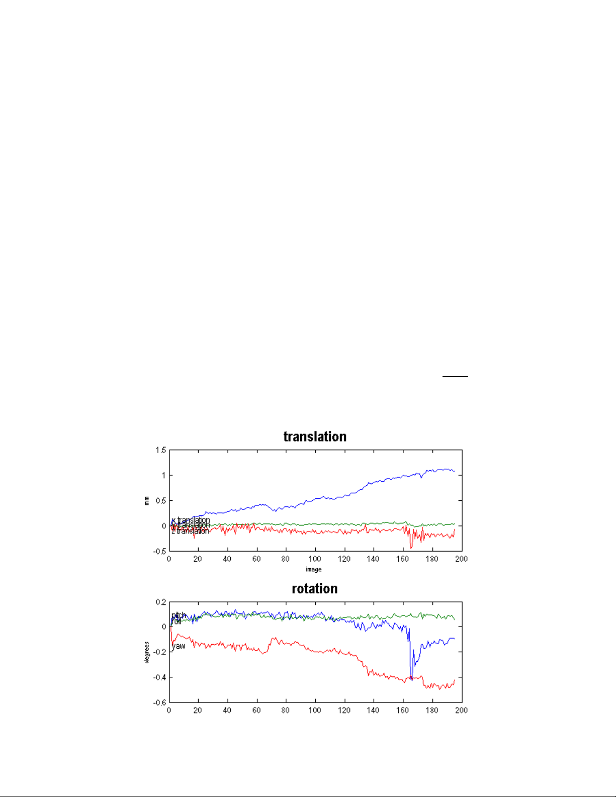
This stage also produces a spm99.ps postscript file, which contains two plots of the
transformations. This file can be viewed using a postscript viewer or can be converted to a PDF
using Adobe Acrobat Distiller. The top plot shows x, y, and z translations, and the bottom plot
shows x, y, and z rotations. Normally translations should be within 2 mm and rotations should be
within a few radians. If there are translations or rotations of more than 10 mm or radians, then
you should seriously consider using your motion correction parameters as confounds in the
statistical analysis. Otherwise, the large motion artifacts could cause signal changes that affect
your model. See example plot below for what to expect. Also, you should NOT see large sets of
consistent values. If a set of continuous scans appear to stay the same in translation or rotation
(straight line on the plot), that means something has gone terribly wrong. This could indicate a
calculation error that resulted in a meaningless loop in SPM computations, or it is possible that
28
Page 29

all those files are merely copies of the same file. If this happens, you need to diagnose the
problem:
One potential reason for this problem, is an error during the volume separation (if you are
using the old “separate and create headers” routine). You can check if this is the problem, by
running separate again, or by using the r2a (rec2analyze) function to separate the volumes. If
this doesn’t work, run a short realignment on a smaller subset of volumes to determine if the
problem is consistent. It is also possible that data was corrupted either in the export process at
the scanner, or in the transfer from Godzilla. Check the data at all stages to make sure this is
not the case. If this is not due to a data handling error, it could be due to a scanner error, and
the data may be irrecoverable. Of course, you should exhaust all options first.
Your realigned volumes at this point (if you elected to reslice) will be saved in the same
directory as your raw (or slice-timing corrected) volumes, using the same filenames, except the
names will be pre-pended with the letter “r” to indicate that these volumes have been realigned.
You can check the quality of the realignment by display a few of the realigned scans (a
few from the beginning, middle and end of the series) using the <Check Reg> button in SPM.
The images will be printed to the SPM graphical output window and you can click around using
the left mouse button to check the quality of the registration, you may want to re-run the
registration using a higher quality interpolation (e.g. if you used Trilinear interpolation, you
should use Sinc interpolation). You can also change the default options in SPM. Under
<Defaults> select Realignment. Change the option for registration quality from 0.5 to 1.0
(slowest, but most accurate). You may also choose to adjust for interpolation <Adjust sampling
errors> to see if it improves the quality of the registration.
At this point, you may compress and save a copy of your motion-corrected volumes
(since this step is the most error-prone and time-consuming) to have a backup in the case of
data loss.
Anatomical Co-registration (Optional)
This step is recommended for single subject studies, as it offers better anatomical
localization of signal differences. It is also recommended for partial brain acquisitions. The idea
is to use the subject’s anatomical scan as a template to overlay functional activation and to
localize signal differences, instead of using a standard template such as the MNI (Montreal
Neurological Institute) or the Talairach
During scanning, you should collect three types of scans:
1. EPI functional scans
2. An in-plane T1-weighted scans with the same parameters as the EPI. You can use a 2D
sequence like a Spin Echo.
3. A high resolution whole brain T1-weighted scan. Typically this scan has an isotropic (or
almost isotropic ~1mm
popular MP-RAGE (M
3
) resolution and good gray/white contrast. An example is the
agnetization Prepared Rapid Acquisition Gradient Echo) 6. A good
MP-RAGE sequence can be used for structural morphometry and gray/white matter
segmentation, but it can also be used as a reference scan for EPI/in-plane T1 coregistration.
5 Talairach, J. & Tournoux, P. (1988) Co-planar Stereotaxic Atlas of the Human Brain: 3-Dimensional Proportional
System: An Approach to Cerebral Imaging. Thieme, New York.
6 Mugler, J. P., III & Brookeman, J. R. (1990) Three-dimensional magnetization-prepared rapid gradient-echo imaging
(3D MP RAGE), Magn Reson Med 15(1):152-157.
5
29
Page 30

Co-registering Whole Brain Volumes
In this step, you co-register the in-plane T1 to the high resolution 3 dimensional T1 scan.
Click on the <Coregister> button in the fMRI switchboard. Select <1> for <number of subjects>.
Select <Coregister only> under <Which option?>. Select <target – T1 MRI> for <modality of first
target> and <object – T1 MRI> for <modality of first object image>. In the SPM selector window,
select the high resolution 3-D T1 scan as your target scan. Select the 2-D in-plane T1 scan as
your object scan. You will be prompted to select other images for your subject. Here you can
select the entire volume of motion-corrected EPI scans (or alternatively you can select you’re
the mean EPI image (other images can be registered at a later point if you desire). Once SPM is
done, you will see the results of the registration in the graphics window. You can also use the
<Check Reg> button to check that the images are registered well.
This procedure works well, because your subject will not move too much between the
EPI scans and the in-plane T1, so the transformation matrix required to bring the in-plane T1 in
register with the high resolution scan can also be used to register the EPI’s.
Co-registering Partial Brain Volumes
If your in-plane T1 and functional scans have partial brain coverage, you can use a
similarity criterion such as Mutual Information (MI)7 to estimate the cost function for the
registration parameters between the in-plane T1 and the high resolution T1. Mutual information
is an information theoretic approach which measures the dependence of one image on another
and can be considered to be the distance between joint distribution (dependence) and the
distribution assuming complete independence. When the two distributions are identical, this
distance (and the mutual information) is zero. Logically, MI works best when there is most
overlap between images, and thus it is ironically less effective at handling partial volume
acquisitions, but it is better than simpler approaches (e.g. minimizing entropy).
To use MI, you must change the SPM defaults to use MI in coregistration. First click
<Defaults> and select <Coregistration> under <Defaults area?>. Select <Use Mutual
Information Registration> when prompted. Mutual Information is a robust similarity criterion
which will eliminate voxels that are not in both images (i.e. not in the partial in-plane T1 but in
the whole brain high resolution acquisition) from the cost function calculations. Now you can go
through the steps in 11.1 exactly the same way as before, but changing this default option will
enable you to co-register a partial brain volume.
Spatial Normalization to Standard Space
Spatial normalization is the process of warping scans from several subjects into roughly
the same standard space to allow for signal average and evaluating results in a group, rather
than an individual. Spatial normalization in fMRI gives us two important advantages:
1. We can determine what typically or generally happens in a group
2. We can report locations of activation (or signal differences) according to Euclidean
coordinates within a standard space, e.g. Talairach and Tournoux space.
Spatial Normalization in SPM is a two-step process. The first involves determining the
optimal 9 or 12 parameter affine transformation that registers the images together. This is
followed by an iterative non-linear spatial normalization using functions that describe global
7 Wells, W. M., III, Viola, P., Atsumi, H., Nakajima, S., & Kikinis, R. (1996) Multi-modal volume registration by
maximization of mutual information, Med Image Anal 1(1):35-51.
30
Page 31

shape differences (not accounted for by affine transformation). The initial affine transform yield
better starting estimates for the nonlinear normalization, which in this case performs well and
achieves a good registration with only a few iterations.
Correcting Scan Orientation
Before normalization, you need to make sure that your scans are in the same orientation
as the template to which you are going to normalize. In SPM 99 and SPM 2, you can set the
defaults to flip the images when being displayed. Because this is just the display mode and not
the actual orientation, I suggest displaying one of your scans in another program that can tell
you the true orientation of the scan, e.g. MRIcro or Measure. In SPM, you want the top left box
to have the coronal view, the top right box to have the sagittal view, and the bottom box to have
the axial view. The eyes in both the sagittal and the axial views should be aimed towards the
coronal view. This means that your scans are in radiological orientation (your left is the subject’s
right, and vice versa), which is SPM’s normalization default, and the default for the EPI
template. It is important that you get your scans in this orientation before you normalize. The
correct orientation should be known before you start pre-processing. Many investigators choose
to use a fiducial marker on the right temple (a small object that is visible on high resolution
scans, to always tell what the subject’s right is). There are two ways of doing this:
1. Reorienting images using <Display>
Click <Display> and select one of the EPI images. If the orientation is incorrect, you may
use defined rotations in pitch, roll and yaw to get it in the right orientation. The most
common issue is the sagittal facing away from the coronal. This can be remedied using a
“pi” orientation in <yaw>. This may take a bit of playing around to get it just right, but
remember that doing this without having a fiducial and knowing the true orientation is
useless. Once you find the correct rotations needed, click on <Reorient images> and
select the rest of the functionals. This will create .mat files for all the functionals with the
new orientation information.
2. Changing the normalization starting estimate defaults
You can also change the defaults for normalization by clicking <Defaults> and selecting
<Spatial normalization> under <Defaults area…?>. Select <defaults for parameter
estimation>. In the estimates options, you can select <Neurological> if that is the correct
orientation of your scan. You can also select custom affine parameters. You can use this
to tell SPM to flip the scans along certain axes. For example [ 0 0 0 0 0 0 1 1 1 0 0 0] is
neurological (R is R), while [0 0 0 0 0 0 -1 1 1 0 0 0] is radiological.
Normalization Defaults
This is a brief explanation of all of SPM’s normalization defaults, for reference only. In
most cases, the defaults preset by SPM will be sufficient for our purposes. Remember that any
changes to SPM defaults will be undone every time you restart SPM. You can access the
normalization defaults, by clicking <Defaults> and selecting <Defaults for parameter
estimation>. The first set of options defines the affine starting estimates and was described in
detail above. The next set of options asks you to select whether or not you would like to allow
<customized normalization>. This basically includes an option to customize the normalization
options (in case you forget to set the defaults). The default is set to <disallow>.
The <number of nonlinear basis functions> is used to further specify how many functions
should be used to warp the scan. The default is 7 x 8 x 7 which for most purposes will be
31
Page 32

sufficient. You may use more or less, depending on the quality of normalization and the scans. If
you choose [ 0 0 0 ] basis functions, SPM will only carry out the affine normalization only,
without using any nonlinear basis functions. You are also given the option to specify the
<number of iterations>. This is the number of iterations of nonlinear spatial normalization. 12 is
the default and in most cases will be enough. If the quality of the normalization is not great, this
number can be increased.
The next set of options have to do with <nonlinear regularization> which is used to
minimize the sum of squared difference between the template and the warped image, while
simultaneously minimizing some function of the deformation field. This is necessary, as without
it, it is possible to introduce deformations that only reduce the residual sum of squares by a
miniscule amount (which can potentially make the algorithm run infinitely). The default here
<medium regularization> is in most cases adequate. If normalization needs more warping, you
can decrease the amount of regularization needed.
The next option <Mask brain when registering> is used to estimate spatial normalization
parameters from a specific region (e.g. a brain mask) or the whole volume. If your signal from
skull and dura is very low, then you can get away with not using a brain mask, but if you want to
exclude any signal from skull and dura, you should select the default brain mask, which is the
image saved in the “apriori” directory of the spm99 directory called “brainmask.img” or a specific
mask (to be specified by you, e.g. a study specific brain mask)
You are also asked if you would like to <Mask object brain when registering?> which is
used in case you want to estimate the normalization parameters from only a limited region of the
object images. This can be used for normalizing brains with lesions (see section 12.3) by
incorporating weighting via an image with values between 0 and 1 that matches the space of the
object image (e.g. an MRIcro mask).
You also have another set of defaults for writing normalized files. Select <Defaults>
again, and select <Spatial Normalization> followed by <Defaults for writing normalized>. The
first option is to specify the bounding box, which is the definition of the volume of the normalized
image that is written (mm relative to the anterior commissure). Leave this as the default [-78:78
-112:76 -50:85]. Under <voxel sizes?> you are given options of the voxel sizes for the
normalized images. The default is 2 x 2 x 2 mm (isotropic) and is in general ok to use for most
studies.
Normalization to a Standard EPI Template
Click <Normalize> and select <Determine parameters only>. Type 1 for <# subjects>. In
the SPMget window, select the first motion corrected functional image in the series (or the mean
functional). You will then be prompted for the <template image>, which should be an EPI
template. You can use the EPI template (MNI) that comes with the SPM99 distribution. This will
produce a single normalized file and a set of normalization parameters (*_sn3d.mat file). You
will see the quality of the normalization in the SPM graphics window on the right. If it looks ok,
you can apply it to the rest of the images. If not, then your orientation may be incorrect and/or
you may need to modify your normalization defaults. Assuming everything looks ok, you can
now click <Normalize> again but this time select <Write normalized only>. When you are
prompted, you can select the normalization parameter set or the *_sn3d.mat file that was
produced in the previous step. In the next window, select the rest of the functional scans.
32
Page 33

Under <interpolation method> you have
the choice between bilinear or sinc interpolation.
If you have used sinc interpolation during
realignment (i.e. when it is most needed) you
can get away with using a less robust
interpolation method during normalization, i.e.
bilinear interpolation. Sinc interpolation will
perform better, but it is generally much slower.
Nearest neighbor interpolation should not be
used during normalization, as it is an overly
simplistic approach (takes the value of the
closest voxel as the value of the desired sample
point, resulting in a very “blocky” image that is
degraded quite considerably). Once all options
are specified, normalization will be underway.
This process will output normalized files resliced
to the selected voxel resolution (i.e. 2 x 2 x 2
mm), which are named using the same prefix as
the source files, except they are prepended with
“n” to indicate that they are spatially normalized.
It is important to note that SPM’s
normalization routines are constrained in
assuming that the template resembles a warped version of the image. Modifications are
required in order to apply this type of normalization to diseased or lesioned brains. The driving
force in the registration is based on minimizing the sum of squared difference between the
voxels in the image and those in the template. This is based only on voxels that are present in
both images, so if a region of the template is not present in your image, then the spatial
normalization will ignore this part of the template, and normalize according to the rest of the
image.
Unfortunately, in practice, this is not always the case. If your scans differ markedly from
the template, e.g. due to susceptibility artifacts or lesions, then you should consider using
masking, before EPI normalization. See special topic on cost function masking for lesion fMRI.
Gaussian Smoothing
This step resembles blurring the image so that it appears more continuous. There are
three main reasons why we smooth functional data. The first is to increase relative signal-tonoise ratio (SNR) by decreasing high frequency noise. This is due to the fact that
neurophysiologic effects of interest extend over several millimeters and is has relatively low
frequency. Smoothing also conditions the data to conform more closely to a Gaussian random
field model, which renders the assumptions of the statistical model to be later specified, more
valid. Finally, smoothing minimizes the effects of inter-subject anatomical differences, which
increases the sensitivity of group analyses to true signal changes.
Click <Smooth> and SPM will prompt you for an appropriate smoothing kernel
<smoothing {FWHM in mm}>. FWHM stands for full-width at half-maximum and it defines the
size of the Gaussian kernel used for smoothing, measured at the mid-point between the base of
the function and its peak. The rule of thumb is that the size of the kernel should be 2-3 times the
33
Page 34

size of the voxel. If you input only one number, SPM will assume an isotropic resolution and use
this value in all three planes. For anisotropic resolutions, you should input a 3 value vector, e.g.
4 4 8, if you desired more smoothing in the in-plane direction (mostly the case). Select all your
normalized functionals to smooth. Smoothing will produce files corresponding to all the
normalized files you selected, prepended with “s” to indicate that they are smoothed.
Keep in mind that now that your data is smoothed, the effective voxel size is different (if
your original voxel size is 3mm and you smoothed with a 6mm kernel, you now have an
effective voxel size of 9mm for conceptual purposes). This is important to keep in mind during
the analysis step, to evaluate the true effect size of activation based on your acquisition voxels.
Summary of Pre-processing Steps
To summarize, the raw time series undergoes a series of pre-processing steps to prepare
the images for statistical analysis. The typical sequence is slice timing correction (for eventrelated data), followed by correction for head motion, normalization to a standard template, and
finally smoothing with a Gaussian kernel. This sequence may need to be altered for a specific
type of study (e.g. a single subject study may not need to normalize and reslice the time
series.), but for most cases, this order should serve as a good reference.
34
Page 35

Statistical Analysis using the General Linear Model
Disclaimer: Statistical analysis in SPM is inherently dangerous! SPM is one of the
easiest fMRI analysis packages to use. However, due to its apparent simplicity, many will
attempt to use it without the required training. SPM STATISTICS ARE NOT SIMPLE even
though it may seem so at first glance. You need to understand the concepts behind the
buttons before you push them. Please use only as a reference and with great caution.
Modeling and Inference in SPM
Statistical parametric mapping (SPM) commonly refers to use of general linear equations
to model parametric distributions. An SPM analysis computes evidence against a null
hypothesis at each voxel.
The general linear model can be thought of as a linear combination of explanatory
variables plus a well-behaved (independently and identically distributed) error term. For example
it can measure a response variable (observation) at a particular voxel Yj, where j = 1, …, J.
For each observation we have a set of L (L < J) explanatory variables denoted by x
where l = 1, …, L. Explanatory variables may be continuous or discrete variables or covariates.
βl are unknown parameters, corresponding to the explanatory variables. The error terms are
assumed to be independent and identically distributed normal random variables.
jl
Yj = x
j1 β1
+…+ x
+…+ x
jl βl
jL βL
+ єj
iid
This can be written in matrix notation as Y = Xβ + є, where Y is the column vector of
observations, X is the design matrix, β is the column vector of parameters, and є is the column
vector of error terms. The design matrix should be a full description of the model, with the
remainder being in the error term. This is where all experimental knowledge about the expected
signal is quantified.
Parameter estimation in SPM is done using ordinary least-squares
have a set of parameter estimates β* = [β*
values are calculated so that Y* = [Y*
,...,Y*L]. The differences between the actual and fitted
1
,...,β*L]. Based on these estimates, fitted response
1
(OLS) fitting. Say you
values (Y – Y*) are the residual errors e = [e1,...eL]. The residual sum of squares is the sum of the
j
square differences between the actual and fitted values, which can be denoted by Σ
j
j=1
e
. This
2
value is a measure of how well the model fits the actual data. The OLS estimates are those
parameter estimates which minimize the residual sum of squares.
Inference in SPM is based on deriving t and F statistics that test for a linear combination
of effects (contrasts), e.g. ON minus OFF. During testing, effects of no interest can be removed.
The idea in SPM is to enter all known information about the effect of interest in the design
matrix, and test the validity of our assumptions using OLS fitting under the general linear model.
The following will be a walkthrough of how this is done in practice.
Model Specification and the SPM Design Matrix
The idea from model specification is to specify the different conditions (or blocks) of
interest in each functional run, and specify the timing parameters that allow SPM to separate
35
Page 36

their temporal effects. SPM uses a graphical user interface that requests several types of
information to specify and estimate this model. Once SPM has specified the statistical model,
based on the information you provide, it creates a file in your current working directory called
SPM_fMRIDesMtx.mat, which is a design matrix file that can be estimated using the subject's
pre-processed data.
Setting Up fMRI Defaults
Before specifying a model, you may need to change some of the default parameters for
statistical analysis in SPM. If you performed slice-timing correction on your data, then you need
to adjust the sampled time bin parameter to reflect that. SPM divides the TR into a number of
time bins (the default is 16). By default, SPM will sample the first time bin in the TR, e.g. If your
TR is 2 seconds, it will only sample the first 125ms. Since slice timing correction involves the
reconstruction of the time series in the real order, the first 125 ms could reflect activation in a
different slice. During slice timing correction we selected the middle slice as our reference slice,
therefore, we should change the SPM defaults so that the sampled time bin is the middle bin (8).
To do this, click on <Defaults> and select <Statistics – fMRI>. Use default options for the
Upper tail F prob. Threshold, and for the number of bins. However, you should change the
sampled bin to 8, instead of the default (16). Remember that these changes are only valid for
the analysis session in context. If you restart SPM, these changes will be lost.
Model Specification
This section will go through specifying a model for a single subject. Note that if all your
subjects underwent the same testing conditions with the same timing parameters (e.g. in an
epoch design), then the process of model specification needs to be done only once. The saved
design matrix file can be applied to any of your subjects.
In the fMRI switchboard, click on “fMRI models” and select “Specify a model”. You will be
asked to specify the <inter-scan interval> (another term for TR or your repetition time). Enter
your TR here in seconds. On the next prompt for <scans per session>, you have to input the
number of functionals per run and the number of runs, e.g. if you ran 3 sessions with 360
timepoints in each, you would enter [360 360 360] without the square brackets. You are then
asked if <conditions are replicated>. If you are using the same conditions in all sessions for
example, you would hit <yes>. You are then asked if <timing/parameters are the same> in all
sessions. If different sessions had different timing parameters (for example, if you had form A
and form B of the task for two consecutive runs), you would hit <no>. In the latter case, you will
have to repeat the following steps for each session separately.
You are then asked to specify the <number of conditions or trials>. This number depends
on how many conditions you would like to analyze. For example, if you had a memory task that
involves both encoding and recall, you may choose to specify 3 conditions (encoding, recall,
rest) or 2 conditions (active memory, rest). Remember that the idea in matrix design is to
provide SPM with all relevant modeling information. In the above case, it is always better to
analyze 3 separate conditions, unless you had reason to believe that there is absolutely no
difference in activation between the two memory conditions.
You are then asked to specify the names of both conditions. If conditions were replicated,
then you only have to do this one. If not, then you have to specify them for each session.
The next step is to specify whether or not you want to use a <stochastic design>. Click
<No>. This type of design defines a variable probability of a given event type at each stimulus
36
Page 37

onset point. For example, the underlying probability of events can be modeled using a sine
wave. The other option is to use a 'deterministic' model, which is the default for an epoch
design. By deterministic we mean that the events are assumed to occur at a pre-specified time
or within a specific block of time. Stochastic designs are only used when a deterministic model
is not possible or inefficient, for example in the context of event-related fMRI. For more
information on this topic, please see Friston et al. (1999)8.
The next prompt will be for <SOA (Stimulus Onset Asynchrony)>. If your conditions all
have the same length, and the inter-trial interval between presentation of trials of the same type
is always the same, then you can select <Fixed>. If you have more than 2 conditions, or if you
have variable timing parameters, select <Variable>. For each condition you specified, you will
be prompted for two things: Stimulus onset vectors and durations. <SOA (scans) for
condition_1> should be specified in scan numbers. This can be thought of as the number of the
image (from your entire dataset) where your condition starts. This can be calculated from your
timing parameters (divide your onset time (in seconds) by your TR and you will get scans. For
example, if blocks of condition 1 start at 8, 24 and 64 seconds, and your TR is 2 seconds, you
would enter [4 12 32] as your onset time vector.
If you selected a fixed SOA, SPM will prompt you for <time to 1
st
trial>, where you should
input the amount of time (in scans like above) until the 1st trial of this type. Typically this will be
the first parameter in your SOA vector of onset times for this condition. If you selected variable
SOA, SPM will inquire whether you are using <Variable Durations> or not. If you want to limit
your analysis to the duration between stimulation and response, then you can say <Yes> and
enter a behavioral response vector (e.g. reaction time) in the next prompt for <durations
(scans)>. If you do not wish to use variable durations, click <no>.
You are then asked whether or not you would like to use <parametric modulation>. For
most cases, click <none>. This is only done to test the effect of a parametric vector on your
conditions, e.g. If you had reason to believe that you reaction times had a direct effect on your
activation, you can enter your reaction time as a modulator. You can model linear or simple
function non-linear (e.g. exponential, quadratic, etc...) relationships.
Next, you will be prompted for your <trial type>. Here the model specification differs
depending on the type of analysis you want. If your design is blocked, select <epoch>, and
under <type of response> select the most basic <fixed response: box-car function>. This
function describes the blocks using a square function modeled by Y = c (constant) for a < x < b
and 0 otherwise.
If your design is event-related, select <events> and under type of response. If you did
not perform slice timing correction, then you should select <hrf with time derivatives>. If slice
timing correction was performed, you can use a naïve hrf model (i.e. hrf <alone>). HRF is a
8 Firston, K.J., Zarahn, E., Josephs, O., Henson, R.N., Dale, A.M. (1999) Stochastic designs in event-related fMRI”.
Neuroimage 10(5):607-619.
37
Page 38
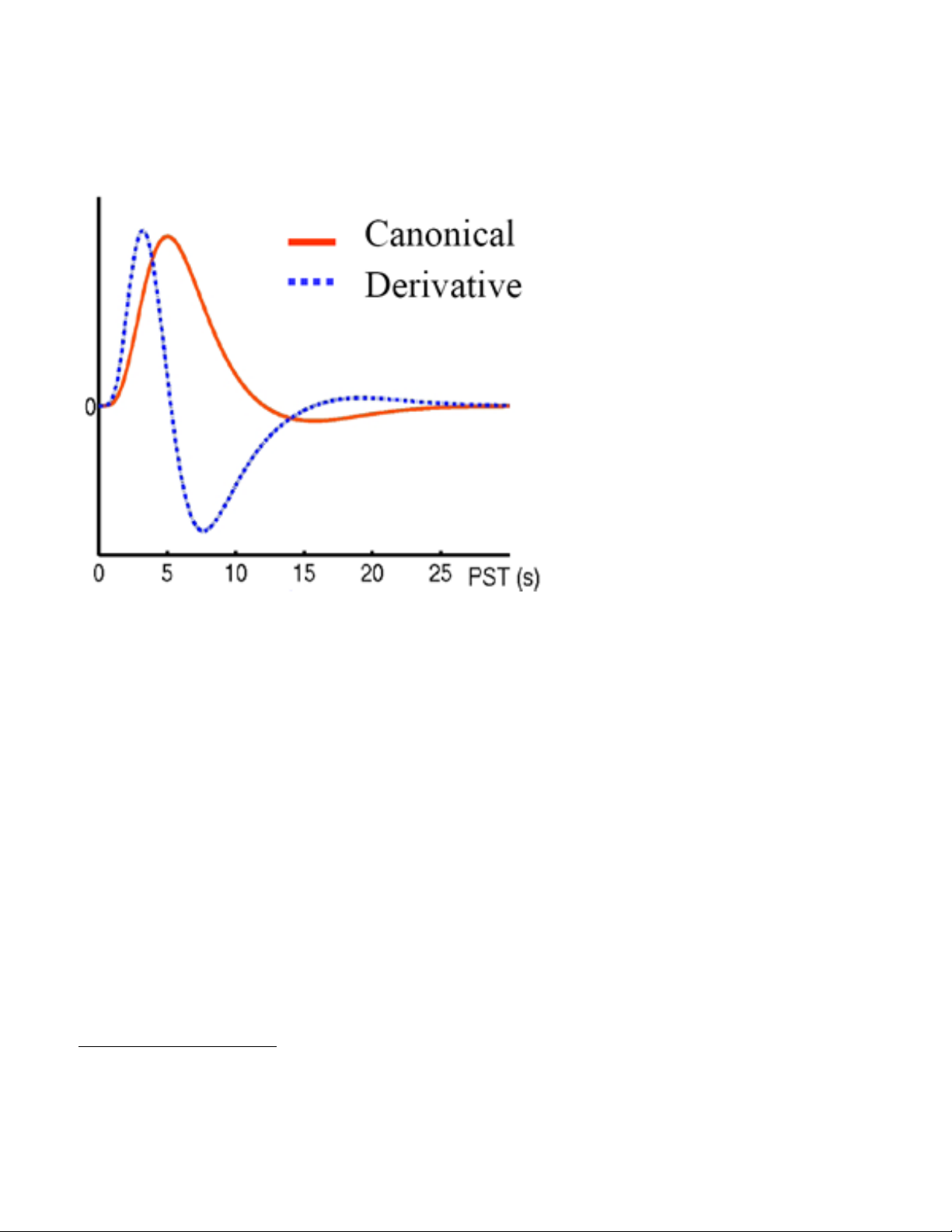
canonical hemodynamic response function that accounts for the lag between the stimulation and
the BOLD signal (see figure below). It is modeled as the difference of two gamma density
functions9.
It is important to note that
each individual hemodynamic
response varies markedly from one
another, but is relatively stable within
an individual 10. It may be preferable
to use empirically derive a subjectspecific HRF during analysis. Details
on this method will be described
later.
If you selected an epoch
design, SPM will ask you separately
about convolving with the hrf and its
derivatives. Modeling temporal
derivatives may be helpful to include
in a model to account for small
delays (or small differences) between
the model and the data, i.e. better
least squares fit, but in most cases, it
decreases the analysis' power. In
other words, if you have no good reason why you should use the time derivatives, it is safest to
stay with a naïve HRF model. Also, these lags are 'tiny' compared with the length of a block, so
that you can always get away with using a naïve HRF model in an epoch design. It may be
helpful to model the time derivatives in an event-related analysis, since timing is more crucial.
If you selected an epoch design, you will be asked for the <epoch length> or the number
of scans per specified condition (durations), if you selected a fixed SOA. You will then be asked
if you want to model <interactions among trials (Volterra)>. This option is useful if you want to
regress our the effect of the interaction from successive trials of the same type, e.g. priming, but
it should be used with caution. The last prompt will ask you for your <user specified regressors>.
This is where you can specify any potential confounds in your analysis, so you can regress them
out of the model. In most cases, you will enter [0]. However, you can model behavioral or
epidemiological variables as covariates. Another good practice is using your motion correction
parameters as confounds. These covariates was saved earlier on during realignment, but can
be entered into the model at this stage (see note on the next page).
In essence, what SPM modeling is doing is calculating a cross-correlation evaluating
the strength of the relationship between your predicted hemodynamic response and the raw
hemodynamic signal (after filtering and adjusting for global variation).
9 Glover, G.H. (1999). Deconvolution of impulse response in event-related BOLD fMRI. Neuroimage, 9:416-429.
10 Aguirre, G. K., Zarahn, E., & D'Esposito, M. (1998). The variability of human, BOLD hemodynamic responses. Neuroimage,
8(4), 360-369.
38
Page 39

Including mot ion parameters as regressors of no interest (optional)
When SPM asks you for user-specified regressors, type 6. Then it will prompt you for the
values – type spm_load in the box. You can then select the realignment_params.txt file
for the session you're currently specifying. The six regressors for each session correspond to
the six columns from the realignment_params.txt file, which are the estimated motion params in
the following directions:, "right", "forward", "up", "pitch", "roll", and "yaw". During the analysis,
you would have 6 more regressors (and 6 more zeros when it comes to specifying the contrast).
Your design matrix will now be displayed in the SPM graphics window. Check it to make
sure all your parameters are correct. There should be a regressor (β) in the model for each
condition specified. There is also a constant regressor (µ) containing the global cerebral blood
flow values to normalize the mean signal value. Your canonical response basis set should be
displayed. You can use the <Explore fMRI design> to browse between sessions and conditions,
and make sure model is specified correctly. Below is an example of a specified design matrix for
an event-related design, with five conditions of interest, and a constant global regressor.
The design orthogonality graph can be thought of a matrix of correlations. Perfect
correlations are indicated by black. Correlations between 0 and 1 are indicated by some shade
of gray (white being a zero correlation). Each parameter perfectly correlates with itself (the black
diagonal). The rest of the matrix describes how correlated the variables are with each other.
Only the top half of the matrix is shown since the bottom is essentially a replication of the top.
Estimating a Specified Model
After you have reviewed your design matrix and determined that it look ok, it is time to
regress the model on the subject's actual data. Select <fMRI models> and select <estimate a
specified model> from the options. In the SPMget file selector window, select the
SPMfMRIDesMtx.mat file from the working directory. Once you hit done, you will be prompted to
select the scans for each subject and session.
39
Page 40

Global Intensity Normalization
In fMRI analysis, we need to distinguish between regional and global activity. Consider
the activation in a single voxel. Some of this activation could be caused by a regional effect, e.g.
auditory cortex being activated in response to an auditory stimulus, or by a global effect, e.g.
The entire brain's activation level slightly rises. In order to differentiate between the two types of
effects, we need to model global effects separately. This enhances the sensitivity and the
specificity of the analysis. Global cerebral blood flow (gCBF) is subject dependent and is the
global average of activations from every intracerebral voxel. You can remove this effect at this
stage in the analysis, or you can model it independently as a covariate using an ANCOVA later.
Let's say you were only interested in regional effects, you would select <scale> when you
are prompted to <remove Global effects>. This will divide the intensity value of each voxel by
the global brain mean. This will reduce inter-subject variability, and enhance the analysis's
sensitivity, but it operates on the important assumption that the global brain mean does not
correlate with the task (which in many cases is not true). If this assumption does not hold true,
applying global normalization can have some unexpected artifactual results (like large areas of
the brain appear as activated). Use this option with great caution!
Temporal Filtering
The next set of option in estimating your model involves filtering the signal for noise.
Experimentally-induced effects are mixed with noise in some frequency bands, and thus the
analysis's sensitivity decreases if the signal is not filtered for noise first. Usually low frequency
signals are caused by non-experimental effects, such as scanner drift and/or physiological noise
(e.g. anxiety). These low-frequency elements can be filtered out using a high-pass filter. This
filter is implemented in SPM using a set of discrete cosine transform basis functions, which are
an invisible part of the design matrix. This means that high-pass filtering during estimation will
result in hypothesis testing taking low-frequency noise into account.
One important caveat is that if the experimentally-induced effects occur in the low
frequency part of the spectrum, that signal will be virtually indistinguishable from noise, and
applying a high-pass filter will effectively eliminate this interesting signal.
Raw signal
Low freq. signal
High freq. signal
Filtered signal
40
Page 41

The choise of high-pass filter should maximize the signal to noise ratio (SNR). SPM
automatically calculates a default cutoff value based on twice the maximum interval between the
most frequently occuring conditions. This is obviously experiment dependent, but may also lead
to significant loss of signal if the experimental design results in increased power at low
frequencies. Under <session cutoff period (secs)>, check that the default value is appropriate
and go to the next step.
The next prompt will ask you for a low-pass filter. You can think of a low-pass filter as a
temporal smoothing function that can get rid of high-frequency noise. Two types of filter have
been suggested. The first is the canonical hemodynamic response function, and the other is a
Gaussian smoothing kernel with a full-width at half maximum (FWHM) of 4-6 seconds. Applying
the HRF filter is advantageous especially for blocked designs with blocks of duration ~25
seconds (HRF power spectrum peak at 0.04-1 = 25 s). To use a low-pass filter, select either
<hrf> or <gaussian> (usually the hrf filter yields better results).
However, it is possible that the high frequency signal components contain interesting
experimentally-induced activation that this type of filtering would eliminate. Another approach is
to use model intrinsic correlation using a 1st order autoregressive AR(1) model. You can
select this option in the next step. AR(1) will estimate the autocorrelation and the noise
parameters based on the covariance matrix after fitting the GLM. The estimates are used to
create the filter, which is applied to the data before refitting the GLM. This process is done
iteratively until the noise is eliminated.
To sum up, if your design is optimized (e.g. rapid event-related designs) it is generally
recommended that you use a high-pass filter (as low-frequency signal components will most
probably be attributable to non-experimental factors. Temporally smoothing data (i.e. Using a
low-pass filter) can make the analysis overly conservative and obscure possibly robust
activations happening at high frequency. Modeling serial autocorrelations, even though it is
theoretically desirable, will also make the analysis overly conservative.
Once you specify your temporal filtering options, SPM will ask you to <set up trial-specific
F-contrasts> which means that SPM will generate F-contrasts for each condition in each
session for you. You may choose to do this yourself manually once the model is estimated. In
this case click <NO>. Now click on estimate <Now> and the model will be estimated.
The following set of files will be written to your working directory.
<beta*.img/hdr>. Each one is for a condition of interest (from the design matrix). These
are images of the parameter estimates, where each voxel has a beta weight for the condition.
Voxels outside of the analysis space are given the value NaN (not a number).
<mask.img/hdr>
. A binary mask image indicating which voxels are included in the
analysis, and which one are not. This is a summary of all masking options (explicit and implicit)
in the analysis).
<ResMS.img/hdr>. This is a map of the estimated residual variance (error).
<RPV.img/hdr>. This is a map of the estimated resels per voxel. The concept of RESEL
(i.e. Resolution element) is explained later in the context of Gaussian random fields and Type I
error correction.
<SPM.mat>
. This is the actual results file that contains the elements of the matrix
structure and the associated betas.
41
Page 42
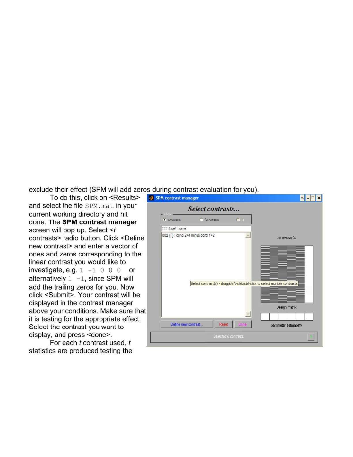
Results and Statistical Inference
Contrast Specification
Once the model is estimated on your data, you need to test for a specific effect of group
of effects, in order to be able to view 'results' so to speak. Remember that results in an SPM
analysis consist of spatially mapped statistical image, where the intensity of individual voxels
corresponds to a t or F statistic. In order to view the effect of a specific condition or relationship,
one needs to specify a “contrast”, which depends on the model specification and on the original
experimental design. For example, if your task consisted of active and rest blocks, you may
choose to look at the 'Active > Rest' contrast. For this you have to construct and test a t
contrast. This process is simple, as a linear contrast is constructed using zeros and ones. Let's
say that your modeled your motion parameters as covariates, and you have two conditions in
the experiment, denoted by ACTIVE and REST. Assuming you specified ACTIVE as your first
condition and you want to look at activation that is present during the ACTIVE condition but not
during REST, you would enter 1 for ACTIVE and -1 for REST. You should also enter zeros for
all of the motion parameters, however since those are at the end of the matrix (i.e. After the
conditions of interest), you can input nothing, and SPM will automatically assume you want to
value of t against the likeliness of its value under the null hypothesis. The t statistic depends on
the standard deviation of the contrast of parameter estimates which depends on the variance in
the regressors. In other words, the t test's sensitivity for estimating a single component in the
matrix is maximized when the rest of the regressors are de-correlated. This test is one-tailed,
testing only for a positive or negative effect. In SPM, you can conduct two-tailed tests testing for
the joint probability of a positive or negative effect, using an F contrast. F contrasts are specified
the same way as t contrasts. A 'F-contrast' may look like
42
Page 43

[-10000
0 1 0 0 0] which would test for the significance of the first or second
parameter estimates. The fact that the first weight is -1 as opposed to 1 has no effect on the test
because the F statistic is based on sums of squares. Once your contrast of interest is specified,
you will be asked if you want to <mask with another contrast>. In most cases, you will select
<No>. However, you can use masking to look at the distribution of activated voxels from either
of two contrasts (inclusive masking) or you can look at the distribution of activated voxels from
both of the two contrasts (exclusive masking)11. The following files will be written to your
directory:
<con*.img/hdr>
. This is a 'contrasted' image, which means it is a weighted sum of beta
images, according to the specified contrast parameter, e.g. 0 1 -1 0 0.
<spmT*.img/hdr>
. This is a voxel-by-voxel t-statistic image. It is formed by dividing the
contrast image by an estimate of the standard error. These images are thresholded and are
used to produce the maximum intensity projection SPM{t}s.
Thresholding and Inference
The next set of options have to do with specifying a threshold for viewing results. By far,
this is one of the most complicated and often debated issues in fMRI analysis, and especially in
the context of SPM. As such is the case, we will take some time to review some of the essential
concepts, before we decide on how to threshold our data.
It is worthy of note that thresholding can be a dangerous science, since it may eliminate
some very interesting findings.
However, without it, one cannot
evaluate the significance of the
results and/or the quality of the test
used to produce them. Let's adopt
the notion that we need to apply
some reasonable threshold before
we view the results, keeping in mind
that looking at unthresholded results
can be very telling in some cases.
Statistical inference in SPM is
constrained by the need to exert
control over Type I and Type II
errors.
Rejecting the Null Hypothesis
Statistics are usually tested
against the null hypothesis (H0),
which is the hypothesis that there is
no finding. Statistical values are
compared to a null distribution, which
is the distribution expected when
there is no effect.
11 You can think of masking in Boolean terms. Inclusive masking is an OR relationship, and exclusive masking is an AND
relationship.
43
Page 44

There are two kinds of errors that can be made in significance testing. The probability of
Type I error is the probability of incorrectly rejecting a true null hypothesis (H0) and is denoted by
the greek letter alpa (α). This is called the Type I error rate. The probability of Type II error is the
probability of incorrectly accepting a false null hypothesis and is denoted by the greek letter beta
(β). This is called the Type II error rate. A Type II error is only an error in the sense that an
opportunity to reject the null hypothesis correctly was lost. It is not an error in the sense that an
incorrect conclusion was drawn since no conclusion is drawn when the null hypothesis is not
rejected. What this translates to in terms of fMRI statistics, is that we only need to correct for
Type I error, when testing for significance.
The situation in fMRI statistics is made more complicated because there are many voxels
in the brain, and thus many statistical values. The null hypothesis therefore refers to finding no
effect in the entire volume of the brain. Now we are asking the question of whether or not a
group (or 'family') of voxels is activated, and the chance of error that we are willing to accept is
the family-wise error (FWE).
Type I Error (Multiple Comparison Correction)
Since the general linear model in SPM is used to test each voxel individually and
simultaneously, then several (hundred) tests are being conducted at once. This means that the
collective alpha (α) value increases. This increases Type I errors. In order to control for Type I
error, we can adjust the alpha value of the individual tests to maintain an overall alpha value at
an acceptable level. This is known as a 'correction for multiple comparisons'.
In theory, uncorrected p-values (significance of finding, without correcting for any multiple
comparisons), can only be used if the investigator had an a priori hypothesis that activation
should exist in a single pre-specified voxel (consider the same for every voxel that is tested).
Since this usually not the case, but rather we would have some idea of which structures should
be activated, correction for multiple comparisons in the appropriate search volume is necessary.
For example, if we expect to find a significant effect in the anterior cingulate cortex, we would
correct for multiple comparisons in the volume of the anterior cingulate (using a prespecified
mask or template). Sometimes, however, we have no idea where we expect to find activation in
the brain. In such a case, we have to correct for multiple comparisons across the entire volume
of the brain. In practice, this is done by choosing a corrected p-value.
Correction for multiple comparisons is possible using a Bonferroni correction. This type
of correction is too conservative, consequently resulting in an increase in Type II errors). It is
also inappropriate for our purposes because it assumes independence between voxels. If
datasets are spatially correlated (which is the case in fMRI), there are fewer independent
observations that need to be conducted.
The SPM alternative is using Random Field Theory (RFT), which provides a way of
correcting the p-value that takes into account the fact that neighboring voxels are not
independent by virtue of continuity in the smoothed functional data. RFT uses the expected
Euler characteristic for a smoothed statistical map. Calculating the expected Euler
characteristic tells us the expected number of clusters above a given threshold, and thus gives
us an appropriate height threshold. First the smoothness of the data is estimated (to figure out
how spatially correlated the statistical maps are). This allows us to calculate the expected Euler
characteristics at different threshold levels. The effect of smoothness and the Euler
characteristic is demonstrated below. Smoothness reduces the chance of noise passing through
the threshold, consequently controlling for Type I errors.
44
Page 45
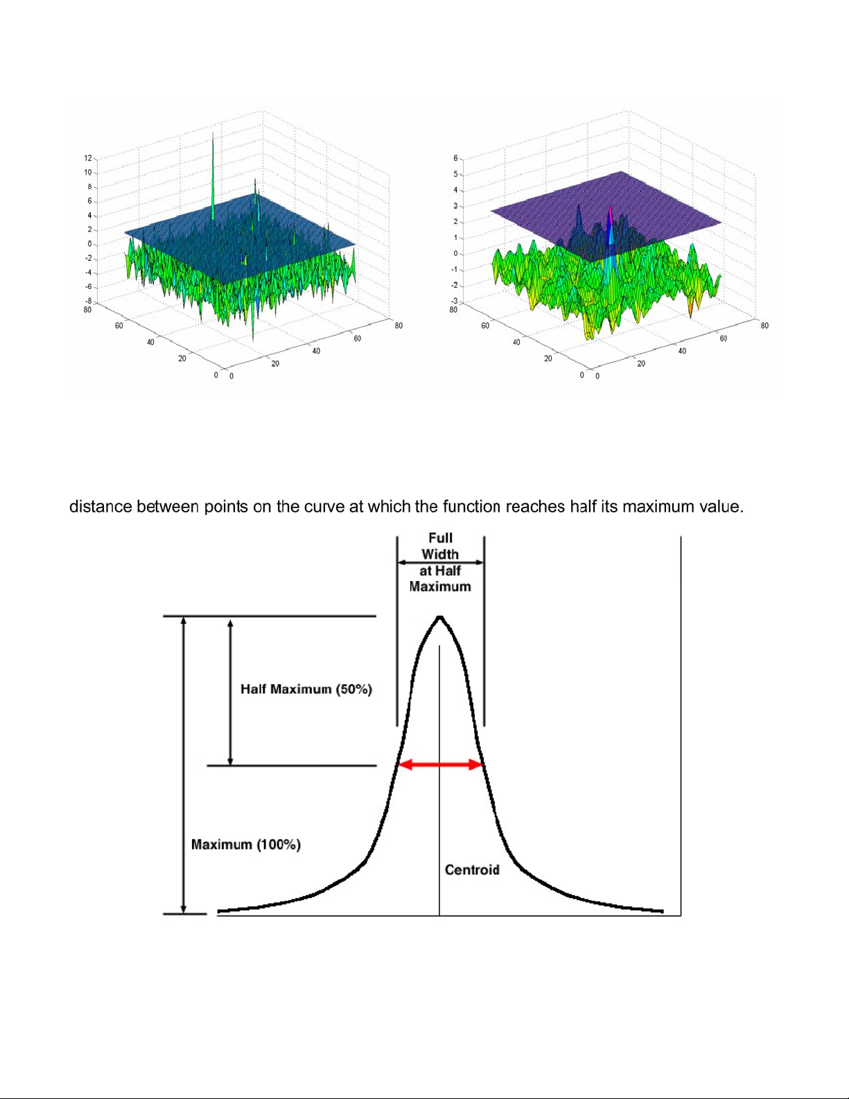
If we had an arbitrary 2-D spatial map of independent values, smoothed with a FWHM of
10 pixels, then we know the smoothness of the data, because it is completely the result of the
smoothing we applied. Smoothness is usually expressed as a FWHM kernel which is a
parameter commonly used to describe the width of a "bump" on a curve. It is given by the
The FWHM is used to calculate the number of Resels (resolution elements) in a
statistical map. This is similar to the 'number of independent observations' in the statistical map
45
Page 46

but is not exactly the same. A resel consists of the number of pixels it takes to create a FWHM
block. For example, if the FWHM kernel is 10 pixels, then a resel is a block of 100 pixels (10 x
10). The number of resels is a useful characteristic to keep in mind when working with smoothed
images. This should be thought of as an alternative to thinking of images in terms of pixels, as
the latter assumes independence between the elements.
At high thresholds, the expected Euler characteristic is almost the same as the probability
of familywise error. So, if we can calculate the expected Euler characteristic, we can predict the
familywise error. Worsley et al. (1992) 12 came up with a formula to calculate the expected Euler
characteristic based on the number of resels in an image. The mathematics are too complicated
to discuss here, but they are described in detail in the above referenced paper. For the most
part, the Euler characteristic yields a good estimate of the error and gives us an adequate
correction for Type I errors. .
In functional imaging it is a little more complicated, since we do not know the smoothness
of the original data (even though we know the smoothing kernel which was applied at the end of
pre-processing). Because we do not know the extent of spatial correlation in the original data,
smoothness has to be calculated from the images themselves. This can be done using residual
values from the statistical analysis. The method is described in detail in Kiebel et al. (1999) 13.
Spatial Extent Threshold (Cluster analysis)
Another way to control errors is to use a minimum cluster size to specify significant
results. This relies on the assumption that areas of true activation will typically extend over more
than a single voxel. SPM asks you to specify an <extent threshold> or minimum cluster size. For
example, if you specify 10, then all clusters less than 10 contiguous voxels in volume will be
rejected as false positives. This means that SPM provides two different ways to control for Type
I errors. Selecting the right threshold once again depends on the smoothness (correlation) of the
voxels. Smoothing increases the needed cluster size (large clusters only will pass the
threshold). However, if voxels are not spatially correlated (data is not sufficiently smooth), then a
smaller cluster threshold is more appropriate. Even a cluster size of 3 reduces Type I error rate
significantly.
Viewing Results using Maximum Intensity Projection
In SPM you are given the option to set a height threshold as well as an extent threshold.
Once both are specified, results are printed in the SPM graphics window and the contrast you
specified is produced as a con_000*.img file to your working directory. The SPM glass brains
show a spatial map of single voxels (or clusters in the case of extent thresholding) which
survived the height and extent threshold. You can print the statistics table to the graphics
window by clicking on <volume> or <cluster> under p-values in the Results window. The table
can also be printed to the Matlab console by right clicking on it and selecting <Print text table>.
The SPM 'glass brains' are viewed using maximum intensity projection (mip) of significant
voxels and clusters in three orthogonal views. The gray scale of the activation for each pixel of
each view of the brain is proportional to the the largest value (be it Z score or F ratio), for the
12 Worsley KJ, Evans AC, Marrett S, Neelin P. (1992) A three-dimensional statistical analysis for CBF activation
studies in human brain. J Cereb Blood Flow Metab. 12(6):900-18.
13 Kiebel SJ, Poline, JB, Friston, KJ, Holmes, AP, Worsley, KJ. (1999) Robust smoothness estimation in statistical
parametric maps using standardized residuals from the general linear model. NeuroImage 10:756-766.
46
Page 47
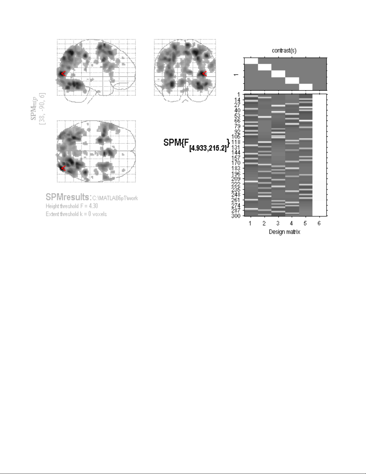
voxel with the maximum intensity, of all the voxels on a line going through the position of that
pixel, perpendicular to the plane of the page. Thus a dark cluster in the temporal lobe on the
coronal view, could be present anywhere from the front to the back of the brain. SPM glass
brains take a little getting used to. Note that you can navigate by clicking and dragging to the
pointer to different coordinate sets. Each view allow you to navigate one of the three axes.
In order to see the SPM statistical table, click on <volume>. In the SPM graphics window,
you will see that corrected p-values are derived for:
1. Set-level inferences: number of clusters above the height and volume threshold
2. Cluster-level inferences: number of voxels in a particular cluster
3. Voxel-level inferences: p-value for each voxel within a cluster
Set-level inferences are generally more powerful than cluster-level inferences and
cluster-level inferences are generally more powerful than voxel-level inferences. However,
voxel-level inferences are more capable of localizing precise activation (specificity), while setlevel inferences are more sensitive to activation. Typically, one can use voxel-level inferences
as they specifies a high degree of anatomical precision.
Note: The SPM results table and MIP brains are surfable. Clicking a row will move the focus to
those coordinates in the MIPs. You can also move the cursor in the MIP to a cluster by clicking
and dragging. Right click in the MIP to activate a context menu to jump to nearest and global
maxima. You can also type the coordinates directly in the SPM results menu (lower left).
47
Page 48

Small Volume Correction and Regional Hypotheses
When making regional inferences in SPM, we often have some idea of where to expect
activation. If our hypothesis involved a single voxel, then we can use an uncorrected p value as
an appropriate alpha. However, more often than not, we make hypotheses involving regions
rather than specific voxels. For example, you could select a box or a sphere as your
hypothesized region of interest. You could also select a search volume based on a specific
image. Small volume correction is available in SPM using the <S.V.C.> button in the Results
menu. Click on <S.V.C> and select an appropriate search volume. For example, if you wanted
to center your search volume around the set of coordinates indicated by the pointer, you can
select a box or sphere large enough to include the surrounding region. If you select nearest
cluster, then you are essentially selecting a functional ROI, which may not be the best way to
approach an ROI analysis. The reason is that you're using results from your whole brain
analysis to guide your ROI analysis. To keep things fair, those two test should be conducted
separately and independently, as the hypotheses being tested in both are different (i.e. Is there
any activation in the brain? vs. is there activation in region X in the brain). More often, you will
want to select <image> and use a predefined region of interest binary mask, to specify the
search region. The results printed to the SPM graphics window will include only clusters in the
search volume space that survive the threshold. As a results, your corrected p-values will now
only be corrected for the defined ROI search volume. This means your control over Type I error
is better, and your significance is thus increased.
Small volume correction is a way to conduct a pseudo-ROI analysis. Since it is still based
on the whole brain analysis, it is not completely blind to its findings. Ideally you would want the
ROI analysis to be conducted separately and independently of the SPM whole brain analysis.
This can be done by masking your results before viewing them or by using another package to
average values over an entire ROI (optimal). Such a functionality is available in the MarsBaR
toolbox which will be described separately in this guidebook.
Extracting Results and Talairach Labeling
One way you can anatomically label your results is using a standardized atlas like the
Talairach Atlas. This is a coordinate-based system that attaches labels to coordinates. However,
the results in SPM are in MNI (Montreal Neurological Institute) space, which is a different
coordinate system. Before we can attach Talairach labels to the results we need to convert the
MNI coordinates to Talairach coordinates. This is typically done using formulas like below.
if z >=0 % This is at the anterior commissure
x_tal = (.99*x);
y_tal = (.9688*y + .0460*z);
z_tal = (-.0485*y + .9189*z);
else
x_tal = (.99*x);
y_tal = (.9688*y + .0420*z);
z_tal = (-.0485*y + .8390*z);
end
The above is how MNI2TAL works. This simple function, written by Matthew Brett can be
downloaded as \\Soma\Software\Matlab\mni2tal.m . An easy way to utilize this script and apply
48
Page 49

it to the entire set of results to prepare a set of Talairach coordinates for further processing is by
using the extractresults script, which can also be downloaded from our internal server as
\\Soma\Software\Matlab\extractresults.m . You need to put both files in your matlab path, and
then in the matlab console, type > extractresults to save all of your local maxima and
their coordinates. The script will produce three text files to the current working directory, (1) the
spm table of results, (2) the extracted SPM (MNI) coordinates, and (3) the corresponding
Talairach coordinates. The coordinate files are in tab delimited format, for easy formatting.
The next step is to attach anatomical labels to the Talairach coordinates. For this we can
use the Talairach Daemon Java server or client. The client resides on your computer, and
maintains a database of coordinates and their corresponding labels, while the server is an
online tool you can use to plug into a net server to download the labels. We often use the client
version, since it does not require a network or Internet connection to work. This can be
downloaded from: http://ric.uthscsa.edu/projects/talairachdaemon.html . The Talairach Daemon
Client will read tab or space delimited records from text files containing lists of Talairach
coordinates arranged in x-y-z order. Or, using the Single Point Processing dialog, one can input
in a single coordinate to label. It will then look up the coordinate in the Talairach Daemon
database for the Talairach label. There are options to search for the single point, search range
or nearest gray matter. The output is written to a file which can be viewed in the program, a
third-party text editor or imported into a third-party spreadsheet.
Once you install the Talairach Daemon, open it, and click on <File>. Select <Open> and
select the text file containing the Talairach coordinates that you produced using extractresults.
Now click on <Option> and select <Database options>. Here you can specify whether you want
to search for the nearest gray matter or specify a search range. This means that if the set of
coordinates does not coincide with a gray matter label (e.g. if the coordinates are in white matter
or CSF), you have the choice of being able to specify a neighboring search range. Lancaster et
al. 14 showed that a 5mm gray matter search range enhances the program's localization ability.
Once the options are set, click on <Process>. A new text file will be saved to your diretory
with the extension .td. The file will contain your Talairach coordinates and the corresponding
anatomical labels. Labeling uses the Talairach Atlas five level labeling. Levels 1 thru 5
adequately describe anatomical locations using gross and specific labels. Level 1 defines left
and right cerebra, cerebella and brainstems. Level 2 defines lobes, while level 3 defines the 55
Talairach structures (e.g. anterior cingulate, hippocampus, etc...). Level 4 is a tissue class
definition of gray matter, white matter, or CSF. Level 5 defines Brodmann areas. The Talairach
daemon will give you all 5 labels for each set of coordinates. Results can then be formatted to
include only relevant data. For example, if you set a specific threshold, you may not need to list
all of the significance values for each set of coordinates.
Time-Series Extraction and Local Eigenimage Analysis
You can extract the raw time series data using the <V.O.I> button (Volume of Interest)
from the Results menu. Click <VOI> and give the region you would like to plot an appropriate
name. This will use the SPM function spm_regions.m to extract the time series of adjusted
data (also known as local eigenimage analysis). Select <don't adjust> if you want to look at the
raw unadjusted timecourse. Next SPM will ask you if you want to apply a filter to the data. If
temporal filtering has already been applied to the data, then you do not need to apply any more
14 Lancaster et al. (2000) Automated Talairach atlas labels for functional brain mapping. Hum Brain Mapp.
10(3):120-31.
49
Page 50
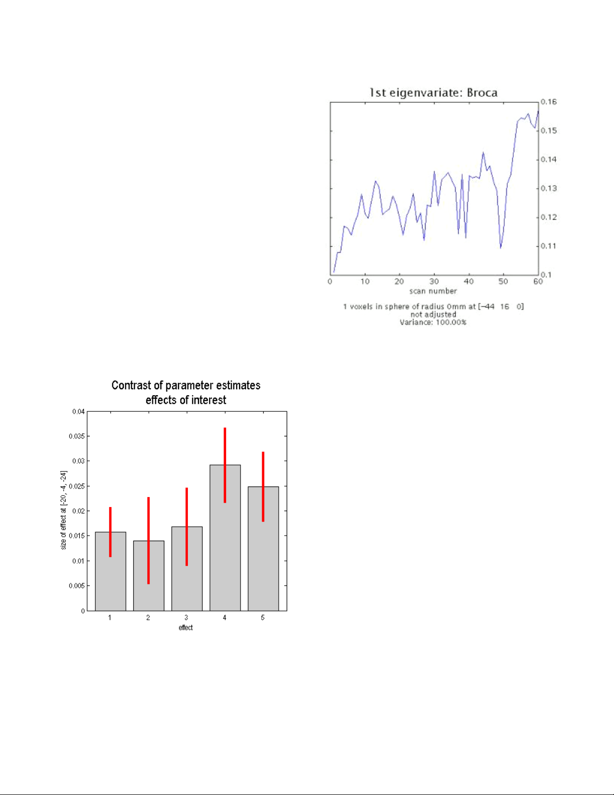
filtering. Select <none>. Now you have to define
your VOI in space. If you select a <sphere> of
radius <0> SPM will extract the results for the
current voxel. You can also select another
geometric shape, e.g. <box> or <sphere> or
<cluster>. The cluster option will select all the
voxels in the nearest cluster for local eigenimage
analysis. SPM will display a graph of the first
eigenvariate of the data centered around the
voxel of 'focus' or the nearest voxel that survived
the threshold. The 1st eigenvariate can be thought
of as a weighted mean of the signal intensity in
the specified space. Extracted VOI data are
saved using the VOI name in the working
directory. For example, if you named the VOI
'areaX', the file VOI_areaX_1.mat would be saved
to your working directory. The variable 'Y' stored
in the Matlab workspace contains all of the
eigenvariate values at every time point in the VOI.
Plotting Responses and Parameter Estimates
Plotting in SPM allows us to attach
numbers to our pretty images. This is very
important as we can pick up on interesting
patterns that the general activation MIPs will not
show. Click <plot> under <visualization> in the
SPM results GUI. Select <contrast of parameter
estimates> and select one or all effects of
interest. A bar graph similar to the one shown on
the left will be printed to the SPM graphics
window. This bar graph tells us how much of the
variance is explained by this particular contrast
(effect size) and the direction of the relationship
(sign) at this particular voxel. The red error bars
are the standard error at the voxel. The size of the
effect is shown as a mean-corrected parameter
estimate. A negative value here does not indicate
a deactivation, but rather a negative deviation
(decrease) from the global mean signal.
When you display a plot in SPM, you can
exert some control on how it is displayed. Checking <hold> in the plot controls menu, will keep
the plot on the screen, so you can overlay another on top of it. Checking <grid> will turn on the
grid. Unchecking <box> will get rid of the black border around the graph. You can use the <text>
controls to change the title and x and y labels. The <attrib> options can be used to change the x
and y axes or return the handle of the current figure to the Matlab console. You can also extract
the numerical data used to build this graph, i.e. beta weights by typing beta in the Matlab
50
Page 51
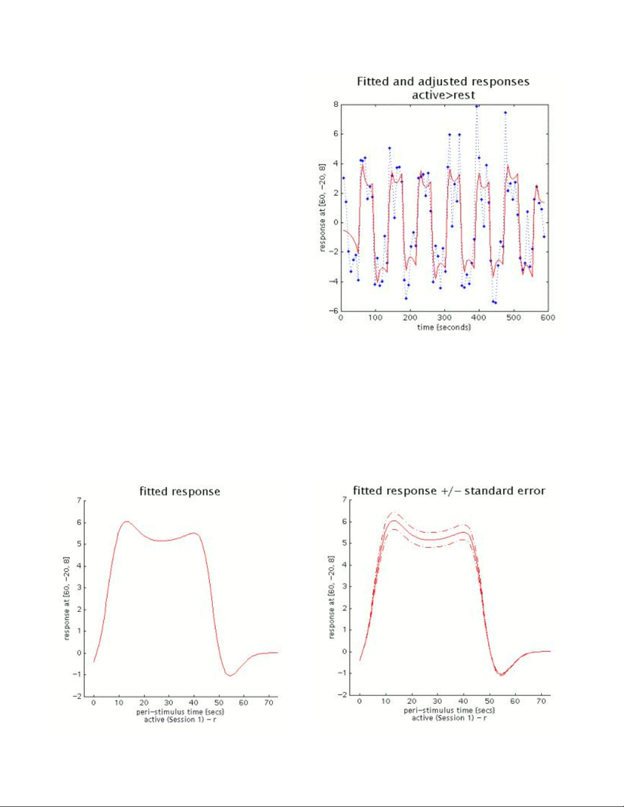
console. The beta weights will be printed in as
a column vector to the Matlab console. An
additional 'large' number will also be printed at
the end of the vector. This number is the
session mean at this voxel. You can type SE
in the console to extract the standard errors.
Click <plot> again and this time select
<fitted and adjusted responses>. Select the
contrast of interest. Usually you will want to
plot the effect against time/scan (especially for
a blocked design) to see how well the model
fits your data. However, if you have an eventrelated design, this type of plot may be less
useful. Select the condition or effect you want
to plot from the list of parameters from the
design matrix. The plot, similar to the one
shown on the right, should show the fitted
responses in red and the adjusted responses
in blue. Adjusted data is data adjusted for
confounding effects like gCBF and hi/lo pass filters. You can extract the adjusted values by
typing 'y' in the Matlab console. Fitted data is the best fit for the specified model with the actual
data. You can extract the fitted values by typing 'Y' in the Matlab console.
You can also plot the individual time components of the series using epoch/event-related
plotting. Click <plot> again but this time select <event/epoch-related responses>. You have
four options. The first option plots the <fitted response>. This is a linear combination of the
regressor (particular condition) multiplied by its parameter estimate. If you choose to plot <fitted
response +/- standard error>, your graph will also include standard error plots. The eventrelated fitted response is the sum of each basis function multiplied by its parameter estimate.
51
Page 52

The last option is plotting the <fitted
response and the PTSH>. PTSH is the peristimulus time histogram, which gives the mean
BOLD signal within a time window after the
occurrence of each event. This models the
waveform of the response. The plot shows the
mean response at each binned time point along
with standard error bars. The fitted response is
the dash-dot line while the PSTH is the solid line.
Essentially this is a plot of the mean regressor
and the mean signal +/- standard error. There is
also no 'baselining' in this plot, meaning that the
amplitude of the waveform for the control
condition has not been subtracted from the
experimental condition. Peri-stimulus time, or the
time that passed since the last presentation of
an event of that particular type is measured in
TR's but to simplify SPM scales it in seconds for
plotting purposes.
Now select <fitted response and
adjusted data>. Select your condition of
interest, and SPM will plot the fitted waveform
(solid line) and the individual data points
(adjusted for confounds). This summary of
the data is helpful, but it should be noted that
this is not the way the SPM analysis is done.
This graph is created by plotting time points
according to the regressor of interest around
the fitted waveform (shape of the modeled
response). This is helpful in evaluating how
well the response model fits the actual data.
The fitted response is based on the data in
the sense that it is the best fit that the model
has with the data, but changes by model or
contrast. Therefore it helps to be able to plot
the actual adjusted data points against it to
get an idea about its accuracy.
Note: Stimulus timing in SPM is computed using stimulus pulse functions, representing the
onset time and duration of each stimulus type. Onset times and durations are specified by the
experimenter in SPM. The user has the option of specifying a finite duration of the stimulus. By
default, however, stimuli are modeled as having zero duration (pulse) and depicted as 'delta
spikes' on the pulse function.
52
Page 53

Anatomical Overlays
SPM offers many way to display your results. The MIP maps on the glass brains are
handy because they show a complete picture of the activation. Another way to show activation
is by using anatomical overlays, which places the activation in a neurological context. However,
one should be careful interpreting overlaid results, because they do not show a complete picture
of the results. In the SPM results window click on <overlays>.
Here you can select whether you would like to present data in the SPM graphics window
on a 3-D whole brain rendering, individual slices (in the z-direction) or using orthogonal sections.
For the rendering, you can use a template from \\spm99\render\. Viewing sections or slices can
be done using any Analyze image. For display purposes you should use a standardized
template, e.g. MNI single subject template under \\spm99\canonical\. Below are some
renderings of activation on anatomical overlays. The slice overlay by z axis is produced using
the script m_slice, written by Kalina Christoff, and can be downloaded from
\\Soma\Software\Matlab\ and is a nice way to represent activation through an entire section of
the brain.
53
Page 54
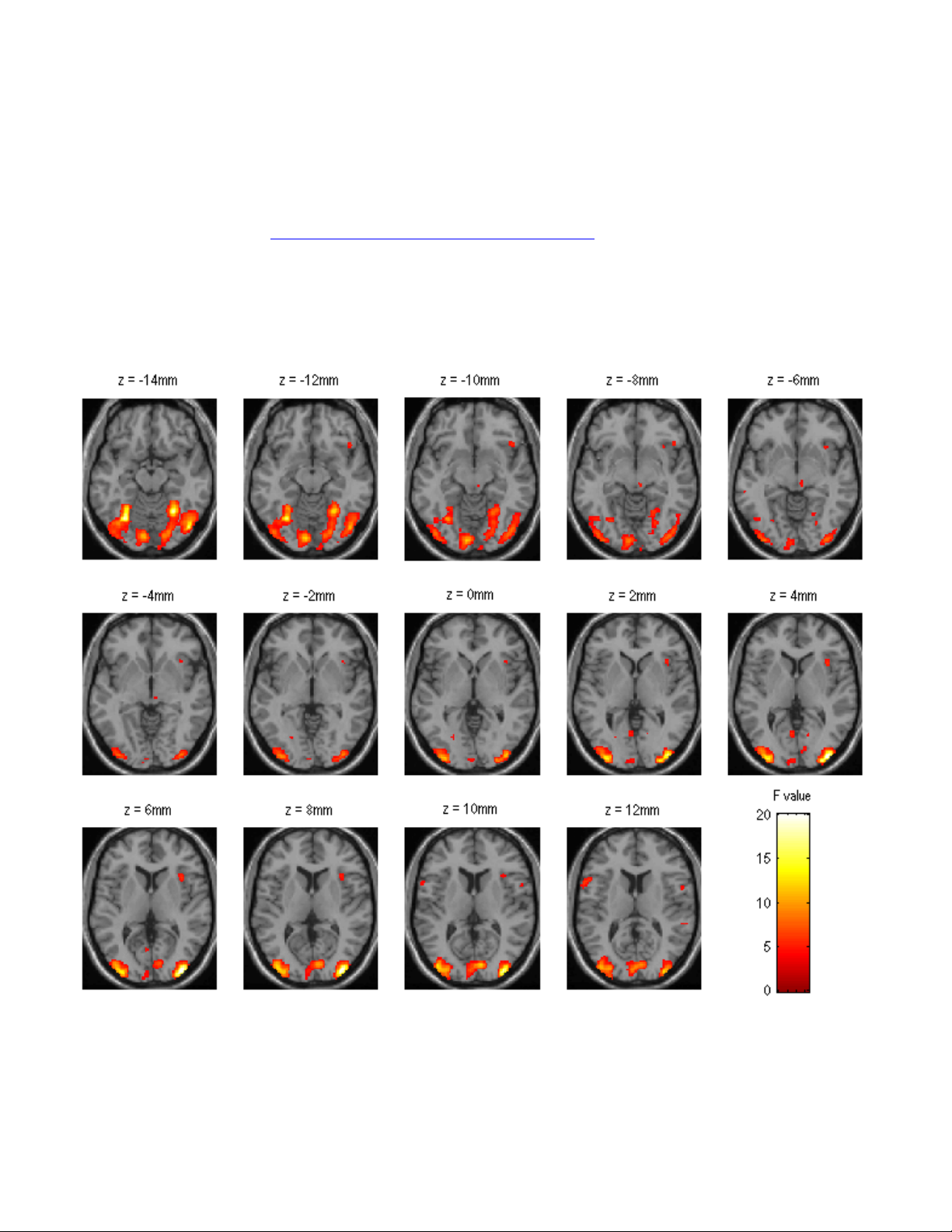
To manually render activations on a brain surface, you can use SPM's rendering facility. Click
the <render> drop-down menu in the fMRI switchboard (not the results context), and select
<display>. Select the number of blob sets you want to render (typically 1 or 2). Select the
spm.mat file containing the results and the appropriate contrast of interest. Give the contrast a
name and do not mask it with other contrasts. Apply the same error correction you applied to
your results and select \\spm99\render\render_single_subj.mat as your render file. Select <new>
for style and <lots> under brighten blobs. The SPM graphics window should be a complete
rendering of the blobs on the single subject MNI brain template. You can save a rendered brain
using <write filtered> in the results menu.
m_slice graphical output
m_slice displays up to 24 transverse slices from the point of focus and increasing along the zaxis (top to bottom). The default max T for the color bar is 7, but you can specify a different T
value. To use m_slice, first you have to make sure that the m file is on your matlab path (you
can do this by placing it in the spm99 directory. Then position your cursor (focus) on the top zslice or the very first image, then in the Matlab window type:
54
Page 55

> m_slice(SPM,VOL,hRef,maxT) replacing maxT with your maximum t or F value.
Editing, Printing and Exporting SPM output
You can edit the SPM output in the SPM graphics window. You can use the top toolbor in
the SPM graphics window to cut, move, and resize items in the window, and add or change text
comments. You can also change the colormap scale for graphics.
<Print>
contents of the graphics window according to the defaults set in spm_defaults.m.
<Clear> clear the graphics window.
<ColorMap> shows options for the different colormap scales. Gray, hot, and pink are
options for displaying 'grayscale', 'hot metal' or 'color' maps. The split settings, e.g. Gray-hot
creates a split colormap to view rendered results.
<Effects> shows available colormap effects. Invert flips the current map, while brighten
and darken will change the lighting of the images using Matlab's routines.
<cut> deletes the graphics object from the page.
<move> repositions graphics and text items on the page using 'drag and drop'.
<resize> resizes the text and graphics objects. Size-up vs. size-down is controlled by
whether or not the 'Shift' button is pressed (holding 'shift' increases the size of the object).
<text> creates an editable text field.
<edit> edits the selected text field.
SPM's default printing mode is postscript. This is a handy mode, because you can print
additional pages of results to the same file (using append). There is a known bug in SPM, where
.ps files are sometimes not written correctly. The reason this happens is that Matlab has another
copy of a spm99.ps in the Matlab\work directory. SPM cannot parse the presence of two
different spm99.ps files and thus does not know where to append the additional pages. This
problem can be fixed by closing SPM and Matlab, and deleting the .ps file in the work directory,
before you restart SPM.
If you want to change the default to print as a tagged image file (tiff) or JPEG, you can do
so from <Defaults> <Printing options> <Other format to file> and select <Baseline JPEG> or
<TIFF with packbits compression>. Print by clicking the <Print> button in the SPM graphics
window. Output is printed to the working directory.
creates a footnote with the username, data and spm version, then prints the
55
Page 56

Region of Interest (ROI) Analyses
In many cases, when we perform an fMRI experiment, we have a specific region of
interest that we hope to activate to a maximal degree using our optimized paradigm. In this
case, using a voxel-wise analysis to look for significance throughout the entire brain is
unnecessary, and decreases our detection ability. Thus, for experiments where we have a
specific regional hypothesis, we require a more targeted analysis.
Anatomical vs. Functional ROIs
One important distinction in our choice of ROI is whether we want to use the subject's (or
atlas) anatomy to determine the relevant voxels for the analysis, or whether we want to use an
actual activation map for this purpose. Functional ROIs, in most cases, should be driven by
independent data. For example, say you conduct an experiment to make sure the hippocampus
is activated during a verbal memory task, and using unbiased analytical methods (whole-brain),
you find robust activation in a locus of the anterior hippocampus or in a region encompassing
the hippocampus and surrounding areas, you can use this activation map as a template ROI for
a different kind of analysis, e.g. Do patients activate their hippocampi to a lesser extent than
controls in response to this task?
Anatomical ROI's are either manually drawn on the individual
subject's anatomical scan (which was acquired in the same session as
the functional scans), and then registered to the EPI scan, or is
extracted from an atlas of brain structures, and placed on the EPI
(after registering the EPI to the atlas space). One such atlas of ROI
labels is the Talairach and Tournoux atlas (shown on the right). Atlasbased ROI's are error-prone, because of the three-dimensional
warping that has to be performed before we can apply atlas labels to
an individual subject's brain. The Talairach brain is not an optimal fit,
since it is based on a single (possibly abnormal) brain scan. An
alternative template is the MNI single subject (scanned 17 times), for
which a labeling atlas is available (The Automated Anatomical
Labeling Atlas – AAL). Manually-drawn ROIs are far more superior
than atlas-based ROI's, but they are much more time-consuming and require expert training to
identify the anatomical markers for a specific brain structure.
Functional ROI's can also be a powerful method, especially for domains where clear
neuroanatomical boundaries are not apparent. A perfect example of this is Nancy Kanwisher's
famous functional “face area”
15
which apparently exists in the fusiform gyrus. This functional
ROI, even though somewhat arbitrary proved useful to alter research using face stimuli.
The MarsBaR toolbox (http://marsbar.sourceforge.net) for SPM uses the AAL labels to
conduct ROI analyses. It also enables us to create functional ROI's based on SPM maps.
15 Kanwisher, N., McDermott, J., Chun, M. (1997) The fusiform face area: A module in human extrastriate cortex
specialized for the perception of faces. J. Neurosci. 17, 4302-4311.
56
Page 57
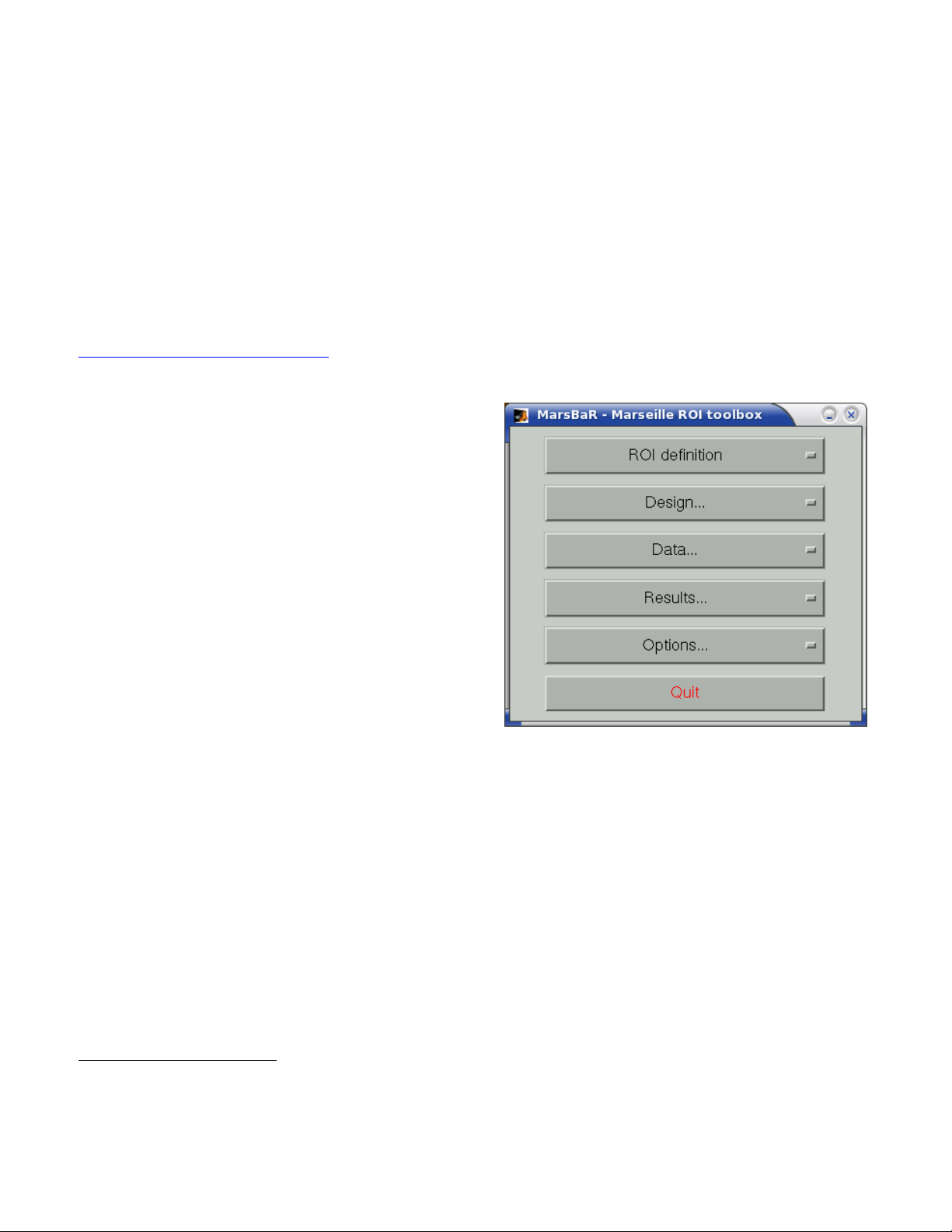
MarsBaR (MARSeille Boîte À Région d'Intérêt)
MarsBaR (MARSeille Boîte À Région d'Intérêt) 16 is a toolbox for SPM which provides
routines for region of interest analysis. Features include region of interest definition, combination
of regions of interest with simple algebra, extraction of data for regions with and without SPM
preprocessing (scaling, filtering), and statistical analyses of ROI data using the SPM statistics
machinery.
Overview of the Toolbox
Installation instructions and tutorials are available on the MarsBaR website at
http://marsbar.sourceforge.net
will only highlight specific features of this package and demonstrate how to conduct a basic ROI
analysis.
First make sure the toolbox directory is on
your Matlab path, and run the command marsbar
from the command prompt. If SPM is already up
and running, the MarsBar window will pop-up on
top of the SPM windows. If SPM is not running,
MarsBaR will start as a standalone toolbox. The
MarsBaR window is shown on the right. The new
version of the MarsBaR does not disable any of the
SPM functionalities. This means that it can run
alongside SPM.
which is also a reference for frequently asked questions. Here I
ROI Definition
Click on the ROI definition menu and you
should get the following options:
View displays one or ROIs on a structural image.
Draw calls up a Matlab interface for drawing ROIs.
Get SPM cluster(s) uses the SPM results interface to select and save clusters as ROIs.
Build gives an interface to various methods for defining ROIs, using shapes (boxes,
spheres), activation clusters, and binary images.
Transform offers a GUI for combining ROIs, and for flipping the orientation of an ROI to the
right or left side of the brain.
Import allows you to import all SPM activations as ROIs, or to import ROIs from cluster
images, such as those written by the SPM results interface, or from images where ROIs are
defined by number labels (ROI 1 has value 1, ROI 2 has value 2, etc.).
Export writes ROIs as images for use in other packages, such as MRIcro.
16 Matthew Brett, Jean-Luc Anton, Romain Valabregue, Jean-Baptiste Poline. Region of interest analysis using an
SPM toolbox [abstract] Presented at the 8th International Conferance on Functional Mapping of the Human
Brain, June 2-6, 2002, Sendai, Japam. Available on CD-ROM in NeuroImage, Vol 16, No 2.
57
Page 58

The following section will show you how to create a functional ROI. Creating an
anatomical ROI is not very different. In fact it is a lot easier than the functional ROIs.
Select <Get SPM cluster(s)...> from the menu. This runs the standard SPM results
interface. Use the file selection window that SPM offers to navigate to the your SPM analysis
directory. Select the SPM.mat file and click Done. Choose a contrast from the SPM contrast
manager, click Done. Then use the same thresholds you used for visualization before. You
should get the familiar glass-brain output in the SPM-graphics window.
Now there should be a new menu in the SPM-input window named <Write ROI(s)>. You
can use this to write single clusters (the one your have selected using the arrows), or to write all
clusters in the SPM. By default MarsBaR saves ROI using the contrast name and coordinates.
Each ROI is then saved as a separate .mat file.
You can now review
the ROI by selecting <View>
from the <ROI definition>
menu. The ROI should be
displayed in a single solid
color on an average
structural image.
The view utility allows
you to click around the image
to review the ROI in the
standard orthogonal views.
You can select multiple ROIs
to view on the same
structural. The list box to the
left of the axial view allows
you to move to a particular
ROI (if you have more than
one). When the cross-hairs
are in the ROI, the
information panel will show
details for that ROI, such as
center of mass, and volume
in mm. The default structural
image is the MNI 152 T1
average brain; you can
choose any image to display
ROIs on by clicking on the
<Options> menu in the
MarsBaR window, then
choosing <Edit Options>,
followed by <Default
structural>. Now we see that
the cluster includes visual
cortex, but there also seems
58
Page 59

to be some connected activation lateral and inferior to the primary visual cortex. The cross-hairs
are between the voxels which seem to be in primary visual cortex and the more lateral voxels.
Ideally we would like to restrict the ROI to voxels in the primary visual cortex. We can do this by
defining a box ROI that covers the area we are interested in, and combining this with the
activation cluster. You can define a box ROI using the <Build> option from the <ROI Definition>
menu.
You can create a box ROI encompassing your interesting activation, and combine it with
your functional cluster using <Transform> from the <ROI Definition> menu. Select <Combine
ROIs> and select the two ROIs. The combine function should be one of the following. You can
any other mathematical operator also.
r1 & r2 (r1 AND r2)
r1 | r2 (r1 OR r2)
r1 &~ r2 (r1 NOT r2)
Now you can write the ROI as an image to use in any other software. Click on <ROI
Definition> followed by <Export>. Select <image> from the menu and choose the ROI to export.
You can select the space for ROI image from the following options:
<Base space for ROIs> this is set by default to the MNI template space but can be
changed from the MarsBaR options.
<From image> here you can specify an individual subject's brain scan for example
<ROI native space> this is the MNI template space. Use only with normalized data.
Running an ROI Analysis
Assuming all the data is preprocessed in SPM, you can use the MarsBaR options to run
the GLM analysis in the same way you would use SPM for this purpose. Under the <Design
menu> you can select <fMRI models>. Here is a summary of the interface (shown on the next
page). The design menu offers options for creating, reviewing, estimating and processing SPM /
MarsBaR designs.
Set design from file option will ask for a design file, and load the specified design into
MarsBaR. The loaded design then becomes the default design
assume that you want to work with this design, unless you tell it otherwise by loading a
different design.
Save design to file will save the current default design to a file.
Set design from estimated; as we will see later, when MarsBaR estimates a design, it
stores the estimated design in memory. Sometimes it is useful to take this estimated design
and set it to be the default design, in order to be able to use the various of these menu
options to review the design.
. MarsBaR will from now on
PET models, FMRI models, and Basic models will use the SPM design routines to
make a design, and store it in memory as the default design.
Explore runs the SPM interface for reviewing and exploring designs.
59
Page 60
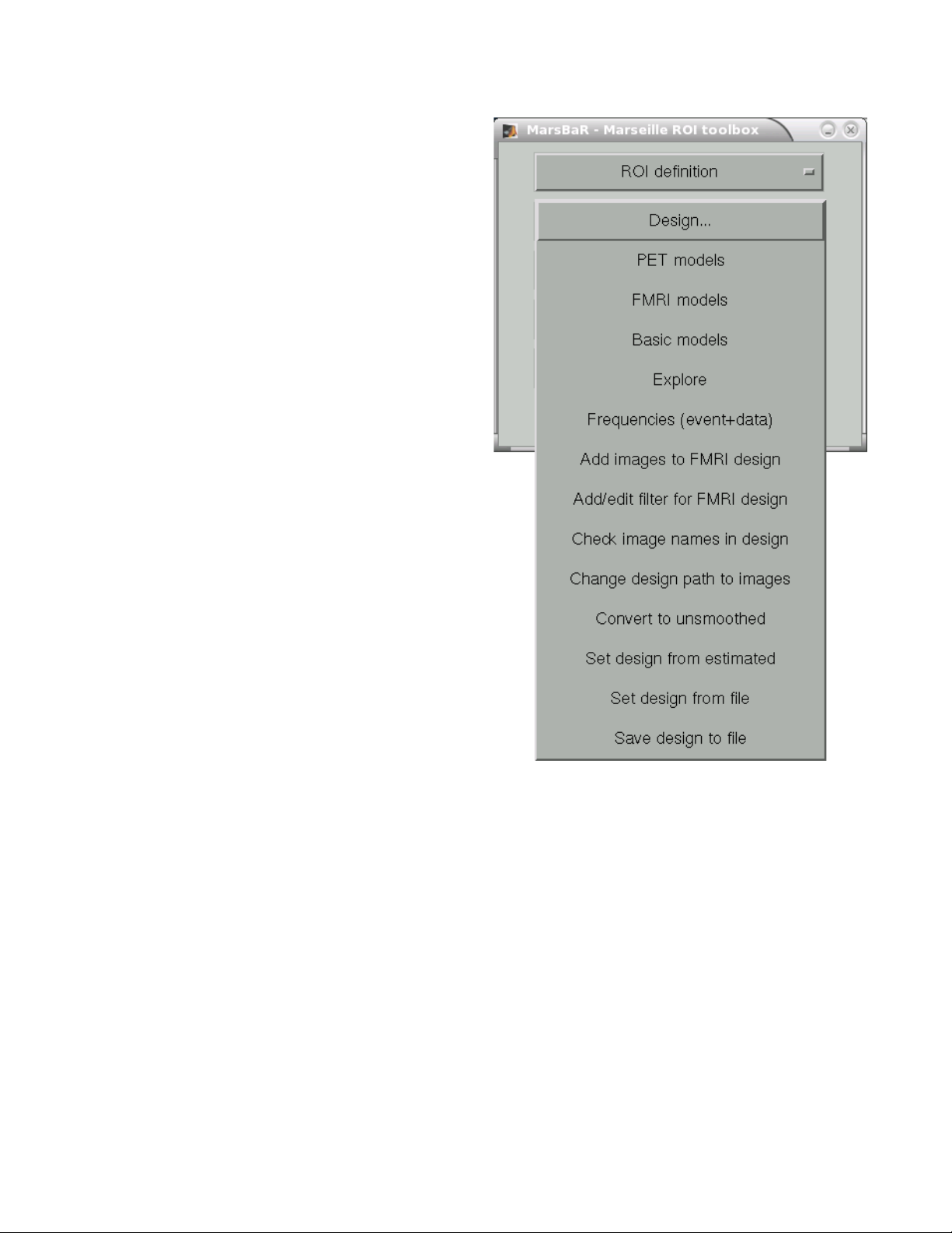
Frequencies (event+data) can be useful
for FMRI designs. The option gives a plot of
the frequencies present in ROI data and the
design regressors for a particular FMRI event.
This allows you to choose a high-pass filter
that will not remove much of the frequencies in
the design, but will remove low frequencies in
the data, which are usually dominated by
noise.
Add images to FMRI design allows you
to specify images for an FMRI design that does
not yet contain images. SPM and MarsBaR
can create FMRI designs without images. If
you want to extract data using the design, you
may want to add images to the design using
this menu item.
Add/edit filter for FMRI design
gives menu options for specifying high pass
and possibly (SPM99) low-pass filters, as well
as autocorrelation options (SPM2).
Check images in the design looks for
the images names in a design, and simply
checks if they exist on the disk, printing out a
message on the matlab console window. A
common problem in using saved SPM designs
is that the images specified in the design have
since moved or deleted; this option is a useful
check to see it that has occurred.
Change path to images allows you to
change the path of the image filenames saved in the SPM design, to deal with the situation
when images have moved since the design was saved.
Convert to unsmoothed takes the image names in a design, and changes them so that
they refer to the unsmoothed version of the same images – in fact it just removes the “s”
prefix from the filenames. This can be useful when you want to use an SPM design that was
originally run on smoothed images, but your ROI is very precise, so you want to avoid running
the ROI analysis on smoothed data, which will blur unwanted signal into your ROI.
For our purposes, all we need to do is set the design file. MarsBaR allows us to directly
import SPM results files (after running the GLM on the individual subject's preprocessed time
series) and extract the ROI data from them. This can be done from the <Data> menu. Here is a
summary of the options.
Extract ROI data (default) takes one or more ROI files and a design, and extracts
the data within the ROI(s) for all the images in the design. As for the default design,
MarsBaR stores the data in memory for further use.
60
Page 61
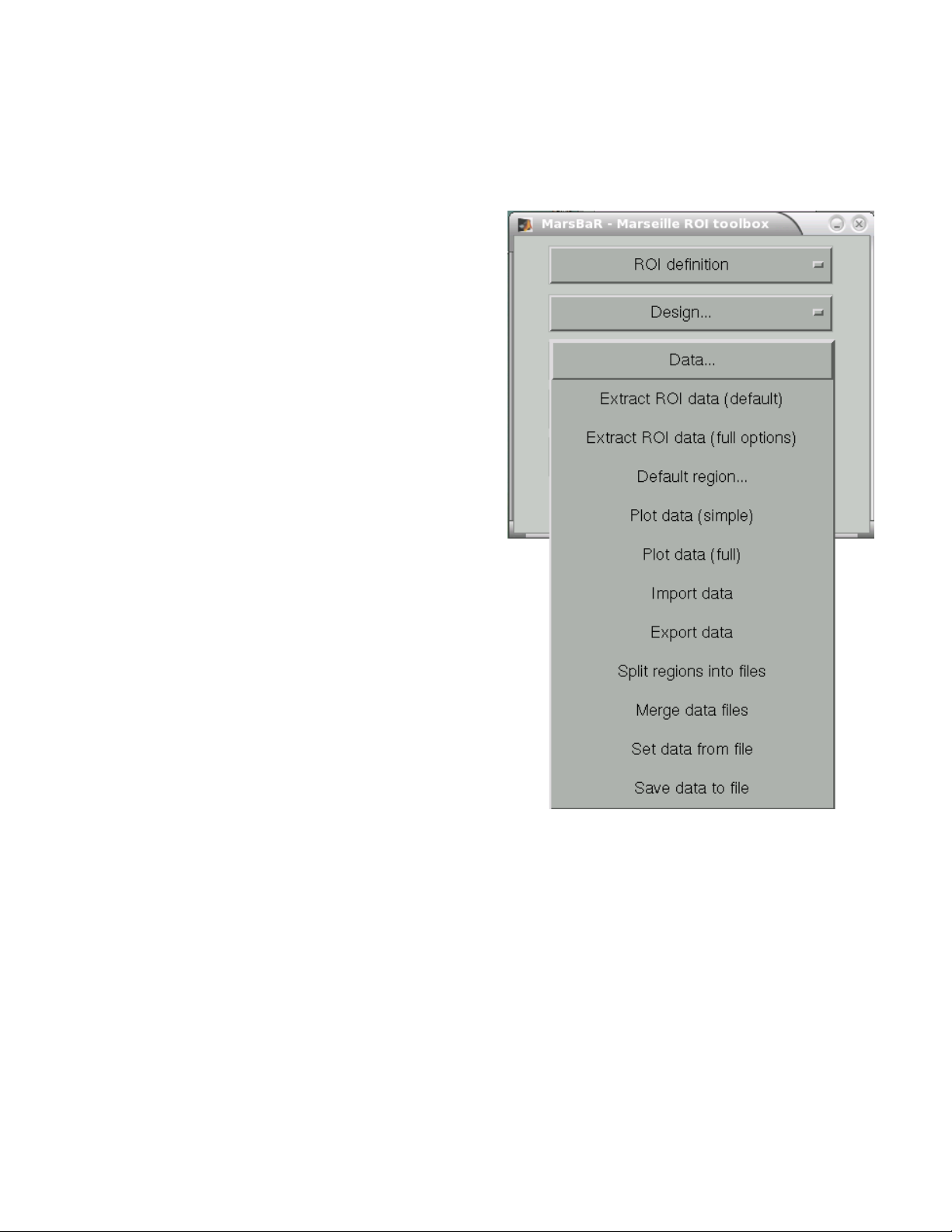
Extract ROI data (full options) allows you to specify any set of images to extract data
from, and will give you a full range of image scaling options for extracting the data.
Default region is useful when you have extracted data for more than one ROI. In this
case you may want to restrict the plotting functions (below) to look only at one of these
regions; you can set which region to use with this
option. If you do not specify, MarsBaR will
assume you want to look at all regions.
Plot data (simple) draws time course
plots of the ROI data to the SPM graphics
window.
Plot data (full) has options for filtering
the data with the SPM design filter before
plotting, and for other types of plots, such as
Frequency plots or plots of autocorrelation
coefficients.
Import data allows you to import data for
analysis from matlab, text files or spreadsheets.
With Export data you can export data to
matlab variables, text files or spreadsheets.
Split regions into files is useful in the
situation where you have extracted data from
more than one ROI, but you want to estimate
with the data from only one of these ROIs. This
can be a good idea for SPM2 designs, because,
like SPM2, MarsBaR will pool the data from all
ROIs when calculating autocorrelation. This may
not be valid, as different brain regions can have
different levels of autocorrelation. Split
regions into files takes the current set of
data and saves the data for each ROI as a
separate MarsBaR data file.
Merge data files reverses the process, by taking a series of ROI data files and making
them into one set of data with many ROIs.
Set data from file will ask for a MarsBaR data file (default suffix '_mdata.mat') and
load it into memory as the current set of data. Save data to file will save the current
set of data to a MarsBaR data file.
For our simple purposes, once again, select <Extract ROI data (default)> and select the
ROI of interest. Once MarsBaR is finished calculating the ROI timecourses, it will calculate a
new summary timecourse for each ROI. This is made up of the means of all the voxel values in
the ROI. Now you can estimate the model on the ROI data using <Results> <Estimate Results>.
You will then be asked to specify a contrast and the analysis will be conducted. You can view
the results by clicking on <Statistics Table> in the <Results> menu. You should see something
61
Page 62

like this:
At the left you see the contrast name. Under this, and to the right, MarsBaR has printed
the ROI label that you entered a while ago. The t statistic is self explanatory, and the
uncorrected p value is just the one-tailed p value for this t statistic given the degrees of freedom
for the analysis. The corrected p is the uncorrected p value, with a Bonferroni correction for the
number of regions in the analysis. In this case, we only analysed one region, so the corrected p
value is the same as the uncorrected p value. MarsBaR (like SPM), will not attempt to correct
the p value for the number of contrasts, because the contrasts may not be orthogonal, and this
will make a Bonferroni correction too conservative.
There is also a column called Contrast value. For a t statistic, as here, this value is
an effect size. Remember that a t statistic consists of an effect size, divided by the standard
deviation of this effect. The value of this parameter will be the best-fitting slope of the line
relating the height of the HRF regressor to the FMRI signal. This effect size measure is the
number that SPM stores for each voxel in the con_0001.img, con_0002.img ... series, and these
are the values that are used for standard second level / random effect analyses.
More detailed information on how to conduct ROI analyses are available on the MarsBaR
website and in the MarsBaR tutorial (from which this section is extracted).
62
Page 63

Group-Level Analysis and Population-level Inferences
Inter-subject Analyses
Combining data from multiple subjects presents an especially challenging problem in
fMRI. It is difficult to match anatomical locations across subjects, due to the large variability in
brain size and shape. This is mostly overcome using a template-based normalization, where
all subjects are warped to fit into a standard space. However, the quality of the group analysis is
limited by the quality of the registration. If there are large differences in the scans, normalization
may not perform well. This is a serious problem, especially for those who are interested in
smaller structures, such as the hippocampus. Approaches that register the major anatomical
landmarks (gyri and sulci) usually do not register the smaller structures as well. Another
approach is using subject-based region of interest analyses to extract the relevant activation,
however there is a problem with combining individual values into a single statistical test.
A more powerful approach that takes regions of interest into account is a multidimensional registration technique in which regions of interest are outlined on individual subjects
and then used to calculate the cost function in the registration. The result is a much higher
quality registration in the regions of interest, but the non-ROI areas are not as well-registered.
This approach only works if one is only searching space for ROI activation and does not care
about activation elsewhere. For more information on this, see work by Stark (ROI-AL)17 and
Miller (LDDMM) 18.
For now we will consider some of the classic ways that data from multiple subjects have
been combined. All of these analyses depend on template-based normalization.
Fixed-Effects Analysis
This is the simplest approach in fMRI analysis and involves combining the time courses
from each subject into one timecourse. This can be thought of as an addition (or averaging) of
subjects. The assumption here is that experimental effects are fixed. In other words, the
experiment is eliciting the same BOLD response in each subject. Thus, this type of analysis
does not address inter-subject hemodynamic variability. Addition of time courses yields a large
number of degrees of freedom (df) and thus improves the test's detection ability. Inter-subject
averaging on the other hand has less df, but it is more consistent, since averaging is less likely
to be skewed by individual subject effects.
Fixed effects models are typically run with less than 15 subjects. It can be run with more
subjects, but would require more computing power, since running a single model for all subjects
requires an incredibly large number of data points to be evaluated. A serious disadvantage to
this kind of analysis is that inferences have to be restricted to the sample tested. Suppose you
test 6 subjects, where two of the subject have a very large effects, whereas the other 4 did not
have an effect at all. Averaging would still show a significant effect, even though it was only
17 Stark CE, Okado Y. Making memories without trying: medial temporal lobe activity associated with incidental
memory formation during recognition.J Neurosci. 2003 Jul 30;23(17):6748-53.
18 Miller MI, Beg MF, Ceritoglu C, Stark C. Increasing the power of functional maps of the medial temporal lobe by
using large deformation diffeomorphic metric mapping. Proc Natl Acad Sci U S A. 2005 Jun 24
63
Page 64
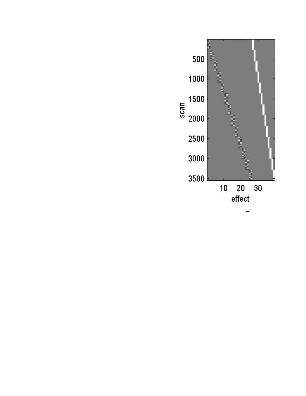
present in less than half your sample. As a result,
inferences cannot be generalized to the entire
population. Fixed effects models can only be used to
estimate sample-specific effects, due to its sensitivity to
extreme effects. Later, we will describe a similar
approach that reduces this problem in fixed effects
modeling.
To put this into practice, there is an easy way to
conduct a fixed effects analysis in SPM. Unlike other
secondary analyses, however, a fixed effects model has
to be run as the primary analysis. After preprocessing all
your data, specify your model as you normally would, but
under <number of subjects> enter the appropriate
number of subjects in your analysis. You will then
proceed to specify parameters for your entire sample.
Once your model is completely specified it should look
something like this (see figure on the right). Now you can
let SPM estimate your fixed effects model, which can
take a couple of days to run on older machines. Fixed
effects models in SPM tend to also crash computers if
then run out of memory. Make sure that your computer is
equipped with enough resources to run such analyses
(... or you can use AFNI instead of SPM!)
Random-Effects Analysis
Random (or mixed) effects analyses are the optimal way to statistical compare subjects
and make inferences about populations, because it accounts for inter-subject variation. This is a
two stage analysis. In the first stage, the hemodynamic response is evaluated for each
individual subject (as described in the modeling section). The secondary analysis uses the
individual statistical maps for voxel-wise activation. The distribution of the individual subjects'
statistics is tested for significance using the general linear model (other approaches, e.g.
Nonparametric testing are also possible as random-effects analyses, but will be described
separately). If the secondary level analysis yield results that are significant at a preset alpha
value, then we can infer that the experimental condition would have had the same effect on the
population from which the subjects were drawn. However, one must remember that if the
sample was not completely random to begin with (e.g. age, gender, education, etc...), then
results cannot be generalized to the entire population. For example, most fMRI studies are
conducted in young, healthy, high IQ college students, which is far from a normal population to
begin with, but is also not representative of the entire population.
Once again, to put words into practice, I will show you how to conduct a random effects
analysis using the SPM machinery. Let's say you conducted an experiment with 20 subjects,
and specified a contrast of interest for each individual (let's say it was con_0002.img/hdr). These
contrast images will be the input data for the secondary analysis. Collect your con_0002 img/hdr
files by copying them and renaming them according to the subject name followed by the
contrast, e.g. 20101_ON.img/hdr. Place them in a new directory for the secondary analysis.
64
Page 65
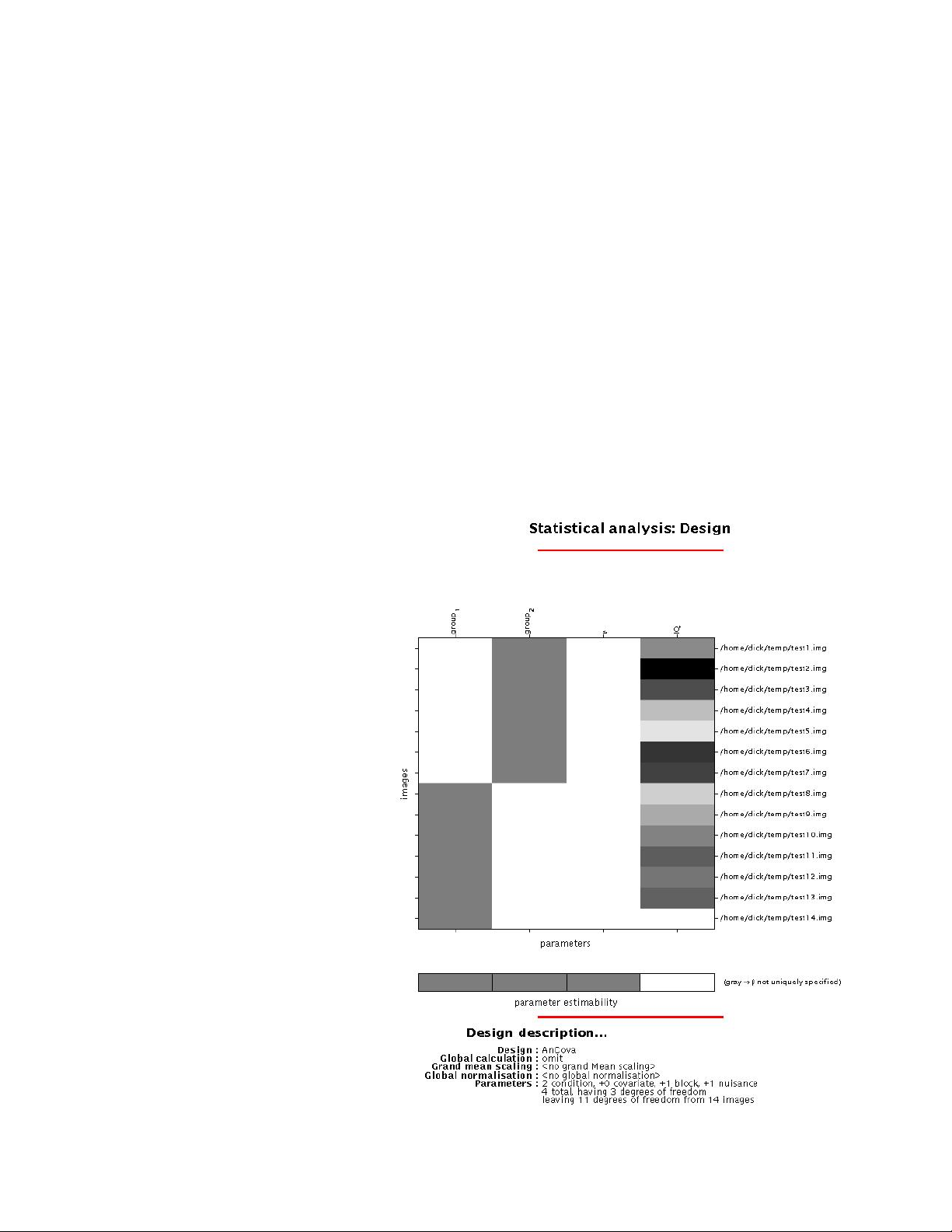
Here is how to conduct simple statistical tests using linear modeling in SPM.
First change your current working directory to the new analysis directory. Now click on
<Basic Models> from the fMRI switchboard, and select <One Sample t-test> from the design
types available. This is the simplest analysis you can conduct, and will evaluate all your subjects
for having a zero effect. Now select all the con_* images from your subjects (only the ones for
the contrast of interest). The next option is for <grand mean scaling>. This scales the overall
mean by a common factor, such that their grand mean is a specific value. If your individual
subject data was proportional scaled (global normalization), then grand mean scaling would be
redundant. Select <no grand mean scaling>. In the next prompt, select <yes> for <implicit
masking>, and this will ignore zero voxel values (the analysis will be faster). In the next prompt
select <no> for <explicit masking>. This option is only used if you are only interested in
calculating statistics in a pre-specified region (a mask). If you select yes, you will be asked to
select a mask image, which will define the analysis space. On the next prompt for <Global
calculation> select <omit>. This is another way to account for global means if you have not done
it before. For our purposes, it is completely unnecessary but should not affect our results. Once
you are done, your model will be shown in the SPM graphics window. Now you can estimate
and view results just like the single subject analysis. All lessons learned from thresholding and
inference apply to group results as well. In fact, this is where they are most applicable, since it is
rarely the case that we will consider
just data from a single subject.
If you want to conduct a <Two
sample t-test>, you would do the
same as above, expect you would
select your con_* images in one
group first, then the other. You will
then be asked to enter a vector that
qualifies group membership (this
vector is made up of 1's and 2's). For
a <paired t-test>, you are asked to
select the pairs on an individual
basis, but all other options are the
same. <One-way ANOVA>'s are
computed in the same manner,
expect you specify two or more
groups individually. <ANCOVA> is
identical but it allows you to enter a
nuisance variable as well (e.g. age,
education,etc...) (see figure).
Simple regressions
<correlations> are the most basic
analyses, and only ask for a single
variable as a linear vector. <Multiple
regression> models are also easy to
apply in SPM, however they are
tricky in several aspects. To develop
65
Page 66

a good MR model, you have to have orthogonal variables, which means that if any of your
variables are correlated, your design will not be optimal. Sometimes, it is good to use something
like factor analysis or principal components analysis first to derive factors that capture the
variability and are least correlated with each other. This improves our testing ability. Also, MR
models can look at interaction terms between variables (e.g. age and performance interaction,
etc...). Once again, multiple regression in SPM is easy to implement, but tricky to design, so
caution should be exercised in developing these models.
In addition to the basic models, you can run any number of higher level models (some
are coded in SPM under the PET category). You can also write your own models in Matlab.
Conjunction Analysis
Conjunction analyses emerged as an alternative which uses all the subjects' activation
maps to estimate activation that is jointly significant in all subjects simultaneously. This
approach benefits from the power of a fixed effects analysis (large degrees of freedom), but
allows us to answer the question (Do ALL subjects activate in this specific location?). Thus,
conjunctions cannot be skewed by one or two subjects, since activation has to be found in all
subjects. However, it still does not allow us to make inferences regarding the population from
which subjects are drawn. Conjunctions allow us to infer that this activation patterns is “typical”
of this population, because a random sampling (provided that sample size is large enough)
showed consistent results.
Conjunctions can be thought of
as a midway solution between
the non-stringent fixed effects
model and the more-stringent
random effects model. In
practice, they are very easy to
do in SPM. First evaluate your
data using a fixed effects model,
including all of your subjects. In
the contrast estimation phase,
specify one contrast per subject
(as if you are looking at each
individual's activation by itself).
Once all contrasts are specified,
select them all using the [Shift]
button, and click <Done> (shown
on the left). Now you can go
through the thresholding
procedure as previously
described. The resulting SPMs
will activation that is common to
all subjects.
66
Page 67

Nonparametric Approaches
Nonparametric approach were introduced as a potential way to assess significance in
fMRI data, because they remove the need to assume that voxels are normally distributed
(Gaussian). This distribution-free procedure is always valid, but requires a lot of computations.
However, by today's standards, these computations are not so time consuming any more.
One such approach uses voxel-level permutation and randomization to investigate
independent observations in neuroimaging studies. SnPM (Statistical Nonparametric
Mapping) is a package that was developed by Andrew Holmes and Tom Nichols as a toolbox
for SPM to conduct these kinds of nonparametric analyses. SnPM uses the GLM to construct timages (or pseudo-t images), which are assessed using standard nonparametric multiple
comparisons procedure. This approach works best for analyses with low degrees of freedom. In
this case, SnPM uses the weighted locally pooled variance estimates (a process known as
variance smoothing), making the approach much more powerful than conventional
approaches that are limited by degrees of freedom.
SPM makes the assumption that data are derived from Gaussian random fields and that
the data is sufficiently smooth and that its properties can be approximated by a continuous
random field. In PET and multi-subject fMRI studies, we have the added problem of low degrees
of freedom, which results in noisy images , due to our inability to estimate variance well from low
df). This affects the t-distribution of the continuous field, against which voxel values are
compared for significance, resulting in a conservative test (underestimates significance).
SnPM is very simple in concept and only makes minimal assumptions regarding the data.
We will consider the multi-subject fMRI example, since it is of most interest to us. In order to test
our hypothesis that there is no experimental effect (null hypothesis), we consider all possible relabellings of subjects and conditions. For example, if we are comparing patients and controls,
we would carry out a randomization test, in which each subject would be reallocated to each
group (resampling). Considering the statistical images associated with all possible re-labellings
of the data, we can derive the statistical distribution of statistic images possible for the data.
Now we test the hypothesis that the result would be an equally plausible statistical image (there
is no experimental effect – the null hypothesis), by comparing the actual labellings of the
experiment with this distribution and compute significance values. Here, SnPM only assumes
exchangeability under the null hypothesis (subjects can be re-labelled if there is no experimental
effect).
Variance smoothing is another powerful tool that we can use in nonparametric testing,
since it allows us to pool variance estimates over neighboring voxels, giving us additional
degrees of freedom. The pseudo-t statistics which smoothed variance have an increased SNR
than the low df t-statistic images. This is another reason why the nonparametric approach is
more powerful.
For a practical guide to SnPM, and to download the software, visit the SnPM main
website at http://www.sph.umich.edu/ni-stat/SnPM/
67
Page 68

False Discovery Rate
False Discovery Rate (FDR) is a new approach to the Multiple Comparisons Problem
(MCP). Instead of controlling the chance of any false positives (as Bonferroni or random field
methods do), FDR controls the expected proportion of false positives among suprathreshold
voxels (rejected tests). A FDR threshold is determined from the observed p-value distribution,
and hence is adaptive to the amount of signal in your data.
FDR is more sensitive than traditional methods simply because it is using a more lenient
metric for false positives. However, if there is truly no signal anywhere in the brain, a FDRcontrolling method has the same control as standard methods. That is, if the null hypothesis is
true everywhere, a FDR procedure will control the chance of a false positive anywhere in the
brain at the specified level. FDR methods therefore exhibit weak control of Family-wise error
(FWE).
The Benjamini and Hochberg FDR method is a straightforward solution to the fMRI MCP
problem, and is implemented in SPM2 and SnPM2. For more details on FDR adjustment, please
see http://www.sph.umich.edu/~nichols/FDR
68
Page 69

Special Topics
Cost Function Masking for Lesion fMRI
This method was developed by Matthew Brett 19 and is explained in detail in the following
section (adapted from Matthew's website). If your functional images differ from the SPM EPI
template that is used for normalization, errors occur in normalization, especially when nonlinear
warping is carried out. To avoid this, you can mask out regions of your functional images you
have the artifacts (or lesions). These areas will not be taken into account during the
normalization. You may want to use the structural images to decide which areas of your
functional images are affected by susceptibility. To do this, co-register your in-plane structural
image to your mean functional image as previously described, and reslice.
Open the images in MRIcro. The easiest way to do this is to double-click on the mean
image and your co-registered structural image in the 'Windows explorer' - this should
automatically open 2 windows of MRIcro, one showing the mean image and the other the
coregistered structural. Yoke both images by ticking the box <Yoke> in the toolbar section
<Slice Viewer>. In the window that shows the coregistered structural, tick the box <Xbars> in
the toolbar section <Slice Viewer>. If you now click on a brain area in the functional image you
will see the corresponding area in the structural (indicated by the crosshairs). Go through all the
slices and mask the lesioned areas in each affected slice. These are areas where you see brain
in your structural images but not your functional images.
To change slices use the scroll bar or the text box immediately under the title ‘Slice
Viewer'. To mask a region, choose the buttons under 'Region of interest'. Find the four lowest
buttons on the right. When you click the first button on the left, the 'closed pen tool' is enabled.
You can draw an outline around a region you wish to mask. If you press the 'shift'-key, you can
delete the outline. When you click the third button on the left, you enable the 'filling tool'. This
allows to fill an outlined region. If you press the 'shift'-key, you can delete the filled area and its
outline.
Alternatively (and more quickly), use the left and right mouse buttons for masking. First
click the 'closed pen tool' (or press F3). Then use the left mouse button to draw an outline and
the right mouse button to fill the outline. If you click into the textbox that specifies the slice
number (underneath the title 'Slice Viewer') you can use the arrow keys of your keyboard to
change slices.
To save the mask, chose "File", "Export ROI as smoothed analyze image". In the next
small window you can choose the smoothing. Choose 8 mm, since this is the smoothing SPM
applies during normalization. The threshold should be 0.001. Keep the default "Adjust sides in
Z-plane only" and make sure that the final drop down box is set for "ROI is 0 [SPM object mask].
You will then be asked to save the roi. Afterwards the mask is saved with the prefix "m" (thus
mmean*.img).
Note that earlier versions of MRIcro do not write mat-files. These contain information
about the image orientation, e.g. the flipping. Therefore it is crucial to provide such a mat-file for
the mask image (the mmean*.img). Copy the mat-file of the mean image (mean*.mat) into the
directory that contains the mask image and rename it by adding the prefix "m". After doing this
19 Brett, M., Leff, A. P., Rorden, C., & Ashburner, J. (2001) Spatial normalization of brain images with focal lesions using
cost function masking, Neuroimage 14(2):486-500.
69
Page 70

you should now have a mask image, header and mat-file with the same name (a mmeana*.img,
a mmeana*.hdr and a mmeana*.mat).
Now you may change the normalization defaults in SPM to allow for object masking. Click
on the <Defaults> button, choose <Spatial normalization>, then <Defaults for parameter
estimation>. Accept all the defaults, except the last two. For the <Mask brain when registering?
> choose <No brain mask>. For the question <Mask object brain when registering?> choose
<Mask object>. Now you can go through the regular normalization steps as above. You will be
asked to select an object masking image, in which case you should select the mmean.img that
you created in MRIcro. This will weigh out the object area and improve the quality of your
normalization.
Advanced Spatial Normalization Methods
In-plane anatomical
This procedure is typically used if the EPI scans have a lot of artifacts. You can choose to
first normalize your in-plane anatomical T1 scan to the standard template, then use those
parameters to normalize the functional scans. Since the T1 was acquired using the same slice
prescription as the functionals, the estimates should be reasonably accurate. To do this, you
would normalize as you normally do, but you would select the in-plane T1 as the image to
determine parameters from, and SPM’s T1 template (under templates) as your target image. If
the normalization quality is reasonable, you can apply the same parameters to the rest of the
functionals. Here you should always use sinc interpolation (9x9x9) even though it is more timeconsuming.
Gray matter segment
Normalizing from gray matter can sometimes increase accuracy, especially for deep
cortical structures, such as the basal ganglia. You can use SPM’s segmentation routines to
produce reasonably accurate estimates of gray and white matter. Click <Segment> in the fMRI
switchboard, and type 1 for <number of subjects>. Select the in-plane MRI scan, and hit
<Done>. When asked <Are they spatially normalized?>, select <No>. Select <T1 MRI> for
modality. You can let SPM attempt to correct for intensity inhomogeneities, since this scan did
not undergo any intensity correction before. Use <lots of inhomogeneity correction> and save
the corrected images. This step will produce three segment files *_seg1, *_seg2, *_seg3 and the
corrected image corr*.img.
Check if you can see skull around the gray matter in seg1 using <Display>. If there is a
lot of skull or dura, you can try to get rid of some of it using SPM’s brain extraction tool. Click on
<Render> and select <Xtract Brain>. Select the gray and white matter segment images, and hit
done. Save the extracted brain. SPM will save it as brain_*.img in the same directory as the
segments. Display the new image to see how much of the skull is gone. If the image seems
reasonable you can use it to mask out the skull from the gray matter segment image (seg1).
Click on <ImCalc> and select first the seg1 image, and then the brain_* image, and hit
done. Name the output filename <*_seg1_noskull.img>. Evaluate the function i1.*i2 (matrix
product of the two images). This will produce a new file with the above filename in the working
directory. You can view it using <Display> to evaluate. If you determine that the segmentation is
successful, you can now normalize the gray matter segment (*_seg1_noskull.img) to SPM’s
<gray.img> template under spm99/apriori. Use the normalization parameter set to normalize the
in-plane functional scans using sinc interpolation.
70
Page 71

Using a Subject-Specific HRF in analysis
The following method is written by Kalina Christoff and describes a method for empirically
deriving a subject-specific HRF based on the work by Aguirre
20
and D'Esposito 21. For this
method to work you must have Kalina's ROI toolbox installed. This can be downloaded at
http://www-psych.stanford.edu/~kalina/SPM99/Tools/roi.html. Installation and usage instructions
are also available on the same page.
During event-related statistical analysis, SPM99 uses a canonical hemodynamic
response function (HRF) to model the occurence of each event. Instead of using a canonical
HRF, identical across subjects, it may be desirable to use a subject-specific HRF in order to
account for differences in HRF across subjects. Since the HRF varies substantially across
people, but is relatively stable for a given person, using a subject-specific HRF may improve the
overall sensitivity of analysis and may be useful in reducing undesirable systematic differences
in HRF between groups (for example, when comparing patients and healthy subjects).
Empirically deriving a subject-specific HRF
Include at the end of your experiment a session during which the subject has to perform a
simple motor or visual task (e.g., finger tapping or watching at a flashing checkboard). This task
should be performed once every 30 seconds, for a brief period of time, e.g., 1 second. For
instance, present a flashing checkerboard for 1 second and a dark screen for the remaining 29
seconds. Instruct your subject to simply look at the screen throughout the session. You could
also instruct the subject to press his thumb and index fingers, for the same duration and with the
same strength, every time he sees the checkerboard, and to remain motionless for the 29
seconds following the checkboard. This should produce robust event-related response in the
primary visual and primary motor cortices. At 3 Tesla, it it is usually sufficient to have 20-30 such
30-second blocks
Once the data have been collected, use the following preprocessing steps: slice timing
correction, realignment with reslicing, and then smoothing. After this, specify and estimate the
statistical model: select no global scaling, high-pass filter 66 sec, low-pass filter 'Gaussian', and
a Windowed Fourier set as basis function set (3rd order and 16 sec window length).
After estimating, open SPM99, and from the RESULTS button, select F-contrasts, and
select 001{F}:effect of interest, hit DONE. Do not mask with other contrasts. Select an
uncorrected height threshold. Use a high F value (e.g., 50). Find an F-value that will give a
cluster in the motor or the visual cortex of approximately 10 cubic cm (e.g., for voxel size 3.75 x
3.75 x 7 mm, a cluster of 100 voxels would be 9.84 cubic cm). After displaying the results with
the chosen F-value, position the cursor on the selected cluster (e.g., the visual cortex), and use
the ROI button with ROI->SAVE COORDS to save the list of coordinates in a file.
20 Aguirre, G. K., Zarahn, E., & D'Esposito, M. (1998). The variability of human, BOLD hemodynamic responses. Neuroimage,
8(4), 360-369.
21 D'Esposito, M., Zarahn, E., Aguirre, G. K., & Rypma, B. (1999). The effect of normal aging on the coupling of neural activity
to the bold hemodynamic response. Neuroimage, 10(1), 6-14.
71
Page 72

Then use ROI->PST PLOT and
enter 'y' to the preprocessing option.
Now go to the matlab console and
type at the prompt:
>>hrf = Cond.Ypr_pst_avg'
>>save visual hrf
Don't forget to put the apostrophe at the
end of the first line. An [n x 1] vector of hrf values
wil be saved, in a variable called hrf in a file
visual.mat in the current directory. This will be
needed during the next stage.
Using the subject-specific HRF during
analysis
Now perform the analysis of your main task, as you would have otherwise, but instead of
selecting 'HRF alone' as a basis function, select the empirically derived HRF. This can be done
either from the interface, or in batch mode. For this option to be available, you will need the
modified spm_get_bf.m which can be downloaded from Kalina's website at http://www-
psych.stanford.edu/~kalina/SPM99/Tools/spm_get_bf.m. Place this file in your matlab path
before spm's original distribution. (It is best to leave the original spm distirbution unchanged,
and install the file in a different directory.)
When working from the interface, load the visual.mat file before specifying the model
(type load visual at the matlab prompt before hitting the fMRI MODELS button) and then enter
the values from the hrf variable when prompted for estimated HRF (simply type hrf).
After specifying the model, but before estimating, please use the EXPLORE DESIGN
button and the design submenu to display the design matrix and basis function for one of the
conditions in order to verify that everything went well. The basis function displayed should have
the same shape as the average plot produced earlier in step 1.
Practical Examples
The benefit from using subject-specific HRF would depend on the extent to which a given
subject's HRF differs from the canonical HRF. In addition, the extent to which this approach
would be beneficial depends on the extent to which the HRF across the entire brain can be
predicted on the basis of the HRF-estimate from the primary visual or motor cortices.
The approach described here uses an estimate of the hemodynamic response in primary
visual or motor cortex to model the the hemodynamic response across the entire brain.
Using subject-specific HRF estimated from primary visual or motor cortex has the
potential problem of inter-region variability. Using a specific function determined from early
cortex doesn't necessarily buy you much unless that's the particular region you are interested in.
To demonstrate, here is data from 9 subjects, for which the hemodynamic response in
the primary visual and primary motor cortices is available. This figure shows the heterogeneity
of the subject-specific HRF from different cortices.
72
Page 73
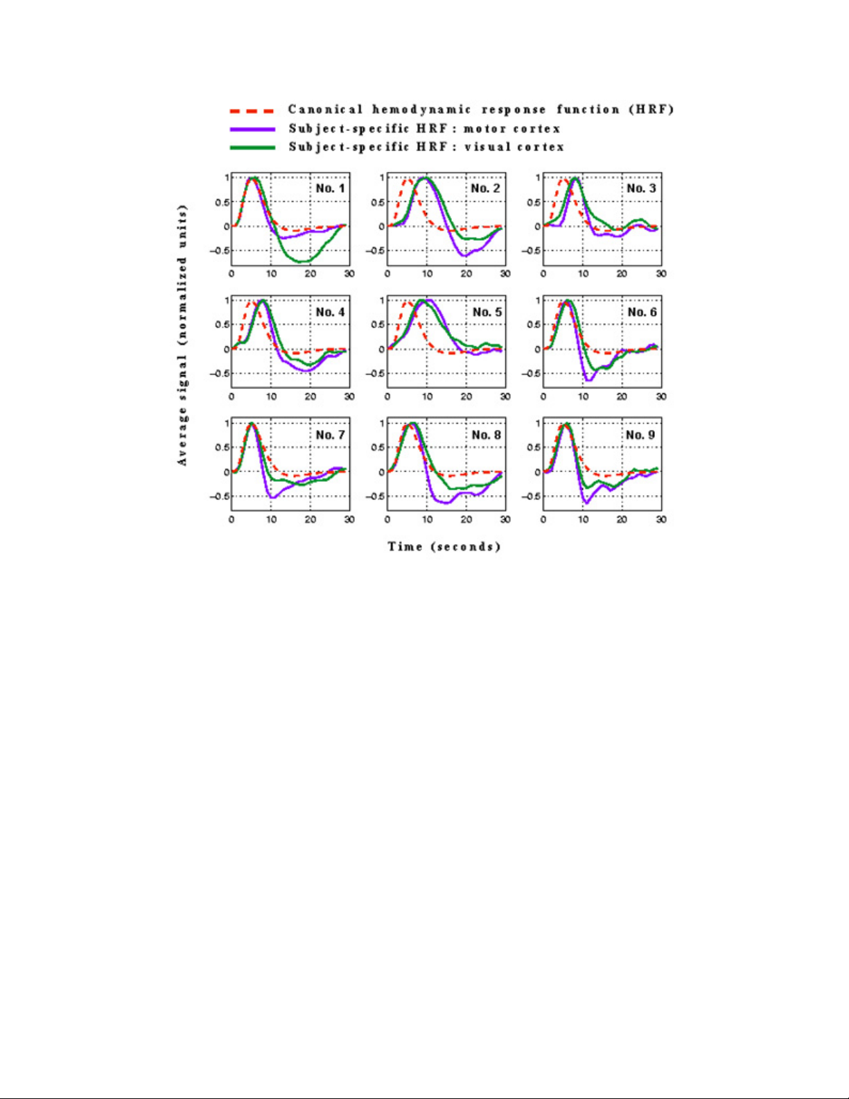
73
Page 74

Guidelines for Presenting fMRI Data
This section is copied from the webpage maintained by Tom Nichols at U. Michigan,
http://www.sph.umich.edu/~nichols/NIpub/ , which is a summary of the discussions on the SPM
mailing list regarding establishing these guidelines. This is a collection of thoughts from active
fMRI researchers, and should be treated as recommendations and not absolute requirements.
However, more and more journals and referees are moving towards making them (at least in
part) a requirement.
At the end of this topic is an example methods section that I wrote to clarify how our
methods should be reported. The reason I did this is because most of the analyses you will be
conducting will take on a simpler form than described in these guidelines, so a lot of this
information may not be completely necessary and/or relevant to your study. Please use the
example section as a guide for the “typical” PNI fMRI study.
Note: Tom’s page is still a work in progress. Please take a moment to visit his site to make sure
you have the most updated version of the guidelines.
General Goal
The goal of this document is to have all neuroimaging papers have sufficient well-reported
methodological detail such that a reader, if presented with an author's data, could reproduce the
same results presented in the paper. A closely related goal is to recommend aspects of the
results that should be reported. The primary goal stated first regards reporting in the methods
section. The secondary goal regards the content of the results section, and possibly an on-line
repository for supplementary data.
Methods: Experimental Design
Number of blocks, trials or experimental units per session and/or subject.
Methods: Data Collection and Processing
Image properties - As acquired
✗ For voxel data (fMRI/PET/SPECT) image dimensions and voxel size.
✗ For fMRI data, additionally, magnet strength (Tesla), TE and TR, FOV, and inter-slice
skip if any; image orientation (axial, sagittal, coronal, oblique; if axials are co-planar w/
AC-PC, the volume coverage in terms of Z in mm); order of acquisition of slices
(sequential or interleaved). Number of experimental sessions and volumes per session.
Pre-processing: General
✗ For voxel data, type of motion correction used (minimally, software version; ideally, image
similarity metric and optimization method used) and interpolation method.
✗ For fMRI, use of slice timing correction (minimally, software version; ideally, order and
type of interpolant used and reference slice).
✗ For fMRI, use of EPI motion-susceptibility correction (minimally, software version).
74
Page 75

✗ The order of the pre-processing steps should be recorded.
Pre-processing: Inter-subject registration
✗ Inter-subject registration method used and software version
✗ Affine? 9 or 12 parameters?
✗ Non-linear? Deformation parameterization?
✗ Non-linear regularization? (E.g. in SPM, e.g. "a little").
✗ Interpolation method?
✗ Object Image information. (Image used to determine transformation to atlas)
✗ Anatomical MRI? Image properites (see above)
✗ Co-planar with functional acquisition?
✗ Segmented grey image?
✗ Atlas information
✗ Brain image template space, name, modality and resolution. (E.g. "SPM2's MNI, T1
2x2x2"; "SPM2's MNI Gray Matter template 2x2x2")
✗ Coordinate space? Typically Talairach, MNI, or MNI converted to Talairach.
✗ If MNI converted to Talairach, what method? E.g. Brett's mni2tal?
✗ How were anatomical locations (e.g. Brodmann areas) determined? (e.g. Talairach
Daemon, Talairach atlas, manual inspection of individuals' anatomy, etc.)
Pre-processing: Smoothing
✗ What size smoothing kernel?
✗ What type of kernel (especially if non-Gaussian, or non-stationary).
✗ Is smoothing done separate at 1st and 2nd levels?
Statistical Modeling: Intra-subject fMRI
✗ Statistical model and software version used (e.g. Multiple regression model with SPM2,
updates as of xx/xx/xx).
✗ Block or event; if block, duration of blocks.
✗ Hemodynamic response function (HRF) assumed or estimated? If HRF used, which (e.g.
SPM's canonical HRF; SPM's gamma basis; Gamma HRF of Glover).
✗ Additional regressors used (e.g. motion, behavioral covariates)
✗ Drift modeling (e.g. DCT with cut off of X seconds; cubic polynomial)
✗ Autocorrelation modeling
✗ Estimation method: OLS, OLS with variance-correction (G-G correction or equivalent), or
whitening.
✗ Contrast construction. Exactly what terms are subtracted from what? It might be useful to
always define abstract names (e.g. AUDSTIM, VISSTIM) instead of underlying
psychological concepts.
Statistical Modeling: 2-level, modality-generic
✗ Statistical model and software version used (e.g. 1-sample t on intrasubject contrast data,
SPM2 with updates as of xx/xx/xx).
75
Page 76

✗ Whether first level intersubject variances are assumed to be homogeneous (SPM &
simple summary stat methods: yes; FSL: no).
✗ If multiple measurements per subject, method to account for within subject correlation.
(e.g. SPM: 'Within-subject variance-covariance matrix estimated at F-significant voxels
(P<0.001), then pooled over whole brain')
✗ Variance correction corresponding to within-subject variance-covariance matrix, so
simply some measure of nonsphericity.)
Statistical Modeling: Inference on Statistic Image (thresholding)
✗ Type of search region considered, and the volume in voxels or mm.
✗ If not whole brain, how region was found; method for constructing region should be
independent of present statistic image.
✗ If threshold used for inference and threshold used for visualization in figures is different,
clearly state so and list each.
✗ Uncorrected inference is not acceptable, unless a single voxel can be a priori identified.
✗ Voxel-wise significance? Corrected for Family-wise Error (FWE) or False Discovery Rate
(FDR).
✗ If FWE found by random field theory (e.g. with SPM) list the smoothness in mm FWHM
and the RESEL count.
✗ If not uniquely specified by use a given software package and version, the method for
finding significance should be described or cited
✗ Cluster-wise significance? If so, list cluster-defining threshold (e.g. P=0.01), and what the
corrected cluster significance was (e.g. "Statistic images assessed for cluster-wise
significance; with a cluster-defining threshold of P=0.01 the 0.05 FWE-corrected critical
cluster size was 103.")
✗ Again, if significance determined with random field theory, then smoothness and RESEL
count must be supplied.
Results
✗ Unthresholded Statistic Maps: Thresholded statistic maps can be seriously misleading.
Both because they exclude sub-threshold but possibly broad patterns, and because they
immediately reveal the mask. A reader automatically equates an absence of
suprathreshold blob with no activation, yet they would think differently if they found there
was no data in that entire region (possible due to susceptibility artifacts)
✗ Time Course Plots: For event-related analyses minimally, and all analyses perhaps,
22
waveforms should be plotted as figures or supplemental materials.
✗ Plotting interactions: If significant interactions (e.g., Group x Condition) or other
complex contrasts are observed, barplots of % signal change or the like would be helpful.
If bar plots are used, error bars should be included. If the contrast is within-subjects
(repeated-measures) the appropriate within-subjects (repeated-measures) errors should
be used
✗ Hemisphere Effects: Inferences about significant hemispheric asymmetry require formal
22 Jernigan, T. L., Gamst, A. C., Fennema-Notestine, C., & Ostergaard, A. L. (2003) More "mapping" in brain mapping:
statistical comparison of effects. Hum.Brain Mapp., 19(2):90-95.
76
Page 77

tests of the Hemisphere x Condition (or Hemisphere x Group) interaction23. It is
inappropriate to infer from main effects (of condition or group) that are significant in only
one hemisphere that there is a significant asymmetry.
✗ Correlation Effects: Analyses of zero-order, partial, or part correlations between brain
activity and other measures (e.g., paper-and-pencil measures, task performance)
mandate the inclusion of scatter plots, preferably with CIs.
✗ Maps of Standard Deviation or Confidence Interval Length: There is also a wealth of
information in the variance or standard deviation. A confidence interval for the primary
effect is a scalar multiple of the standard deviation image (or, even if the CI is desired for
the BOLD %change, it's very easy to compute).
✗ ROI Mask Data: The exact values in a ROI mask can be critically evaluated to see if the
regions covered make sense.
✗ Statistical Diagnostics: To assess if the data satisfy the statistical assumptions, show
the diagnostic statistics that assess Normality and white noise (possibly after whitening)
assumptions.
✗ Design Matrices & Contrasts: When complex designs are used, a graphical
representation of the matrix and a description of contrasts in term of columns could be
provided as supplementary information.
Acknowledgments
The following people have made contributions to this effort. Max Gunther started the thread on
the SPM list, and Karsten Specht, Russ Polldrack, Kent Kiel, Mauro Pesenti, Jesper Andersson,
Iain Johnstone, Robert Welsh, Dara Ghahremani, Alexa Morcom, and Lena Katz, Daniel (aka
Jack) Kelly, Cyril Pernet and Alex Shackman followed with more suggestions.
Last modified: Tue Mar 8 09:32:53 EST 2005 Tom Nichols nichols@umich.edu, UM Biostatistics
23 Davidson, R. J., Shackman, A. J., & Maxwell, J. S. (2004). Asymmetries in face and brain related to emotion. Trends
Cogn. Sci. 8(9):389-391.
77
Page 78

Sample fMRI Methods Section
Scan acquisition
Data were acquired on a 3 Tesla Philips Intera system (Philips Medical
Systems, Best, The Netherlands) at the F.M. Kirby Functional Imaging Research
Center (Kennedy Krieger Institute, Baltimore MD). The system is equipped with dual
Quasar gradients (80mT/m at 110 mT/m/s or 40 mT/m at 220 mT/m/s). A standard
head coil was used to limit head motion. A sagittal scout (localizer) scan was collected
to pinpoint the exact location of the brain. Functional scans were collected using
echo-planar imaging (EPI) and a blood oxygenation level dependent (BOLD)
technique with repetition time (TR)=1000 ms, echo time (TE)=34 ms, flip angle
(θ)=90o, field-of-view (FOV) 240 mm2 in the xy plane, and matrix size =64x64,
reconstructed to 128x128. Thirty four coronal slices were acquired with a 2.5 mm
thickness and an inter-slice gap of 0.5 mm, oriented perpendicular to the anteriorposterior commisure (AC-PC) line. Slices were acquired sequentially along the z-axis;
yielding total volume coverage of 119 mm. Functional scanning was performed in two
sessions, each with 360 timepoints. Total functional acquisition time was 12 minutes.
A high resolution whole-brain anatomical scan was obtained using a T1-weighted, 3D
MP-RAGE (Magnetization Prepared Rapid Acquisition Gradient Echo) sequence with
the following parameters: TR=8.6 ms, TE=3.9 ms, FOV=240 mm, θ=8o, matrix size
=256x256, slice thickness=1.5 mm, 124 slices.
Data pre-processing
Data pre-processing was conducted on a Windows XP workstation, equipped
with dual processors and 2GB of RAM. Statistical Parametric Mapping (SPM99,
Wellcome Department of Imaging Neuroscience, University College, London, UK)
was used, under the MATLAB 6.1 (The Mathworks, Sherborn, MA, USA)
programming and runtime environment. Slice timing correction was conducted using
the middle slice (#16) as the reference slice, and sinc-interpolation. Rigid-body
registration (motion correction) was performed by realigning the scans from both
sessions to the mean image of all the functionals in both sessions. This was conducted
using a 6-parameter affine transformation (3 translations and 3 rotations in x,y, and z
axes), followed by reslicing using a ‘windowed’ sinc-interpolation. Realignment output
plots and realigned volumes were checked for motion artifacts and size of
transformations. Affine (12 parameter) and nonlinear normalization using 7x8x7 basis
functions and medium nonlinear regularization were conducted to deform each
subject’s data into standard space (Montreal Neurologic Institute (MNI), McGill
University, Montreal, Canada) . Template space was defined by SPM’s standard EPI
3
template (MNI). Data were resliced to isotropic voxels (2mm
) using trilinear
interpolation, and spatially smoothed with a full-width at half-maximum (FWHM)
isotropic Gaussian kernel of 5mm3.
78
Page 79

Statistical Modeling and Analysis
Individual subject-level analysis
Individual time series analysis was conducted using the general linear model
within the framework of statistical parametric mapping (SPM99). Data were modeled
as event-related, and convolved with SPM’s canonical hemodynamic response
function (HRF) to account for the lag between stimulation and the BOLD signal.
Motion correction parameters were entered into the model as covariates. The model
was estimated using SPM’s standard ordinary least squares (OLS). Stimulus onset times
and corresponding reaction times were used to define two conditions (ON and OFF).
The contrast of interest subtracted activation during the OFF condition from the ON
condition.
Whole brain random effects
A 1-sample t-test was conducted using the unthresholded contrast image (ON
minus OFF) from each individual using SPM99’s basic modeling facility. Voxel-wise
threshold for inference and visualization using SPM's maximum intensity projections
to p=0.05, corrected for family-wise error (FWE) (5 mm FWHM smoothing and 4016
RESELS), with a spatial extent threshold k of 100 voxels. A Monte Carlo simulation
(AFNI, AlphaSim) was conducted on each threshold pairing (height and extent) to
determine the level of alpha significance. Unthresholded statistical maps were also
produced to check any broad patterns excluded by the thresholding process. The
coordinates of voxels that survived the statistical threshold were produced in MNI
space and converted to Talairach space (Talairach & Tournoux 1988) to facilitate
anatomical labeling, which was conducted using the Talairach Daemon software
(Lancaster et al. 1997) with an adaptive gray matter search range of 5mm3 (Lancaster et
al. 2000). Labels were manually checked with the Talairach and Tournoux atlas
(Talairach & Tournoux 1988)
Region of interest analysis
A 1-sample t-test was independently conducted on the unthresholded SPM
contrast images using the MarsBar toolbox for SPM99 (Brett et al. 2002). This analysis
was limited to a specified region of interest, defined by a robust manual segmentation
of the left and right hippocampus by an expert rater (see Honeycutt et al. (1998) for
details on the method's validity and reliability) on an average T1-weighted template of
all subjects in the study (normalized to SPM space and smoothed with a 4mm kernel).
The model evaluated voxels for significance above a p<0.05 threshold and presence
inside the search region space. Results were corrected for multiple comparisons within
the ROI search region (384 voxels in the left hippocampal space, and 356 voxels in the
right hippocampal space).
79
Page 80

Notes
-------------------------------------------------------------------------------------------------------------------------------
-------------------------------------------------------------------------------------------------------------------------------
-------------------------------------------------------------------------------------------------------------------------------
-------------------------------------------------------------------------------------------------------------------------------
-------------------------------------------------------------------------------------------------------------------------------
-------------------------------------------------------------------------------------------------------------------------------
-------------------------------------------------------------------------------------------------------------------------------
-------------------------------------------------------------------------------------------------------------------------------
-------------------------------------------------------------------------------------------------------------------------------
-------------------------------------------------------------------------------------------------------------------------------
-------------------------------------------------------------------------------------------------------------------------------
-------------------------------------------------------------------------------------------------------------------------------
-------------------------------------------------------------------------------------------------------------------------------
-------------------------------------------------------------------------------------------------------------------------------
-------------------------------------------------------------------------------------------------------------------------------
-------------------------------------------------------------------------------------------------------------------------------
-------------------------------------------------------------------------------------------------------------------------------
-------------------------------------------------------------------------------------------------------------------------------
-------------------------------------------------------------------------------------------------------------------------------
-------------------------------------------------------------------------------------------------------------------------------
-------------------------------------------------------------------------------------------------------------------------------
-------------------------------------------------------------------------------------------------------------------------------
-------------------------------------------------------------------------------------------------------------------------------
-------------------------------------------------------------------------------------------------------------------------------
-------------------------------------------------------------------------------------------------------------------------------
-------------------------------------------------------------------------------------------------------------------------------
-------------------------------------------------------------------------------------------------------------------------------
-------------------------------------------------------------------------------------------------------------------------------
-------------------------------------------------------------------------------------------------------------------------------
80
 Loading...