Fluke MDA-550/FPC User manual

190 Series III

ScopeMeter® Test Tool

Models 190-062, -102, -104, -202, -204, -502, -504, MDA-550-III

Users Manual

É

August 2021 (English)
© 2021 Fluke Corporation. All rights reserved.
Specifications are subject to change without notice.
All product names are trademarks of their respective companies.

Find Quality Products Online at: [e-mail]

www.GlobalTestSupply.com

LIMITED WARRANTY AND LIMITATION OF LIABILITY

Each Fluke product is warranted to be free from defects in material and workmanship under normal use and
service. The warranty period is three years and begins on the date of shipment. Parts, product repairs, and
services are warranted for 90 days. This warranty extends only to the original buyer or end-user customer of a
Fluke authorized reseller, and does not apply to fuses, disposable batteries, or to any product which, in Fluke's
opinion, has been misused, altered, neglected, contaminated, or damaged by accident or abnormal conditions of
operation or handling. Fluke warrants that software will operate substantially in accordance with its functional
specifications for 90 days and that it has been properly recorded on non-defective media. Fluke does not
warrant that software will be error free or operate without interruption.

Fluke authorized resellers shall extend this warranty on new and unused products to end-user customers only
but have no authority to extend a greater or different warranty on behalf of Fluke. Warranty support is available
only if product is purchased through a Fluke authorized sales outlet or Buyer has paid the applicable
international price. Fluke reserves the right to invoice Buyer for importation costs of repair/replacement parts
when product purchased in one country is submitted for repair in another country.

Fluke's warranty obligation is limited, at Fluke's option, to refund of the purchase price, free of charge repair, or
replacement of a defective product which is returned to a Fluke authorized service center within the warranty
period.

To obtain warranty service, contact your nearest Fluke authorized service center to obtain return authorization
information, then send the product to that service center, with a description of the difficulty, postage and
insurance prepaid (FOB Destination). Fluke assumes no risk for damage in transit. Following warranty repair, the
product will be returned to Buyer, transportation prepaid (FOB Destination). If Fluke determines that failure was
caused by neglect, misuse, contamination, alteration, accident, or abnormal condition of operation or handling,
including overvoltage failures caused by use outside the product’s specified rating, or normal wear and tear of
mechanical components, Fluke will provide an estimate of repair costs and obtain authorization before
commencing the work. Following repair, the product will be returned to the Buyer transportation prepaid and the
Buyer will be billed for the repair and return transportation charges (FOB Shipping Point).

THIS WARRANTY IS BUYER'S SOLE AND EXCLUSIVE REMEDY AND IS IN LIEU OF ALL OTHER
WARRANTIES, EXPRESS OR IMPLIED, INCLUDING BUT NOT LIMITED TO ANY IMPLIED WARRANTY OF
MERCHANTABILITY OR FITNESS FOR A PARTICULAR PURPOSE. FLUKE SHALL NOT BE LIABLE FOR
ANY SPECIAL, INDIRECT, INCIDENTAL OR CONSEQUENTIAL DAMAGES OR LOSSES, INCLUDING LOSS
OF DATA, ARISING FROM ANY CAUSE OR THEORY.

Since some countries or states do not allow limitation of the term of an implied warranty, or exclusion or limitation
of incidental or consequential damages, the limitations and exclusions of this warranty may not apply to every
buyer. If any provision of this Warranty is held invalid or unenforceable by a court or other decision-maker of
competent jurisdiction, such holding will not affect the validity or enforceability of any other provision.

11/9 9

Find Quality Products Online at: [e-mail]

www.GlobalTestSupply.com

Table of Contents

Title Page

Introduction.......................................................................................................... 1

Contact Fluke ...................................................................................................... 3

Safety Information ............................................................................................... 3

Specifications ...................................................................................................... 3

Unpack the Test Tool Kit ..................................................................................... 4

How to Use the Test Tool .................................................................................... 6

Test Tool Power ........................................................................................... 6

Test Tool Reset ............................................................................................ 7

Menus........................................................................................................... 8

Key Illumination ............................................................................................ 9

Input Connections......................................................................................... 10

Scope .................................................................................................... 10

MDA Test Tool....................................................................................... 11

Probe Type Setup......................................................................................... 12

Input Channel Selection ............................................................................... 13

View an Unknown Signal with Connect-and-View™ .................................... 13

Automatic Scope Measurements.................................................................. 14

Freezing the Screen ..................................................................................... 15

Average, Persistence and Glitch Capture .................................................... 15

Using Average for Smoothing Waveforms ............................................ 15

Smart Average....................................................................................... 16

Persistence, Envelope and Dot-Join to View Waveforms ..................... 16

Glitch Display......................................................................................... 17

High Frequency Noise Suppression...................................................... 18

Waveform Acquisition................................................................................... 18

Set the Acquisition Speed and Waveform Memory Depth .................... 18

AC-Coupling Selection .......................................................................... 19

Reversing the Polarity of the Displayed Waveform ............................... 19

Variable Input Sensitivity ....................................................................... 19

Noisy Waveforms .................................................................................. 20

Mathematic Functions +, -, x, XY-mode ................................................ 20

Mathematic Function Spectrum (FFT)................................................... 21

Waveform Comparisons........................................................................ 22

Pass - Fail Tests........................................................................................... 24

Waveform Analysis....................................................................................... 24

i

Find Quality Products Online at: [e-mail]

www.GlobalTestSupply.com

190 Series III

Users Manual

Automatic Meter Measurements (190-xx4) ................................................... 24

Meter Measurement Selection ............................................................... 24

Relative Meter Measurements ............................................................... 25

Multimeter Measurements (190-xx2)............................................................. 27

Meter Connections ................................................................................. 27

Resistance Value Measurement ............................................................ 27

Current Measurement ............................................................................ 28

Auto/Manual Range Selection................................................................ 29

Relative Meter Measurements ............................................................... 30

Recorder Functions .............................................................................................. 31

Recorder Main Menu..................................................................................... 31

Measurements Over Time (TrendPlot™) ...................................................... 31

TrendPlot Function ................................................................................. 31

Recorded Data Display .......................................................................... 32

Recorder Options ................................................................................... 32

Turn Off the TrendPlot Display............................................................... 33

Recording Scope Waveforms In Deep Memory (Scope Record).................. 33

Starting a Scope Record Function ......................................................... 33

Recorded Data Display .......................................................................... 34

Scope Record in Single Sweep Mode.................................................... 34

Triggering to Start or Stop Scope Record .............................................. 34

TrendPlot or Scope Record Analysis............................................................. 35

Replay, Zoom and Cursors................................................................................... 36

Replay the 100 Most Recent Scope Screens................................................ 36

Replay Step-by-Step .............................................................................. 36

Replay Continuously .............................................................................. 37

Turn Off the Replay Function ................................................................. 37

Capturing 100 Intermittent Signals Automatically................................... 37

Zoom on a Waveform.................................................................................... 38

Cursor Measurements................................................................................... 39

Horizontal Cursors on a Waveform ........................................................ 39

Vertical Cursors on a Waveform ............................................................ 40

Cursors on a Mathematical Result (+ - x) Waveform ............................. 41

Cursors on Spectrum Measurements..................................................... 41

Rise Time Measurements ...................................................................... 41

Waveform Triggers............................................................................................... 43

Trigger Level and Slope ................................................................................ 43

Trigger Delay or Pre-Trigger.......................................................................... 44

Automatic Trigger Options............................................................................. 45

Edge Triggers................................................................................................ 46

Noisy Waveform Triggers....................................................................... 46

Single Event Acquisition......................................................................... 47

N-Cycle Trigger ...................................................................................... 47

External Waveform Triggers (190-xx2).......................................................... 48

Pulse Triggers ............................................................................................... 49

Narrow Pulses ........................................................................................ 49

Missing Pulses ....................................................................................... 50

ii

Find Quality Products Online at: [e-mail]

www.GlobalTestSupply.com

ScopeMeter® Test Tool

Table of Contents

Memory and PC................................................................................................... 51

USB Ports..................................................................................................... 51

USB Drivers.................................................................................................. 52

Save and Recall ........................................................................................... 52

Save Screens with Associated Setups ......................................................... 53

All Memories in Use............................................................................... 54

Editing Names ....................................................................................... 54

Save Screens in .bmp Format (Print Screen)............................................... 54

Delete Screens with Associated Setups....................................................... 55

Recall Screens with Associated Setups ....................................................... 55

Recall a Setup Configuration........................................................................ 56

View Stored Screens .................................................................................... 56

Rename Stored Screens and Setup Files .................................................... 57

Copy/Move Stored Screens and Setup Files................................................ 57

FlukeView™ 2 Software ............................................................................... 58

Computer Connection................................................................................... 58

WiFi Connection ........................................................................................... 59

MDA-550-III Test Tool ......................................................................................... 60

Motor Drive Input .......................................................................................... 62

Voltage and Current .............................................................................. 62

Voltage Unbalance ................................................................................ 63

Current Unbalance ................................................................................ 64

Harmonics ............................................................................................. 64

Motor Drive DC-Bus ..................................................................................... 66

Voltage DC Level................................................................................... 66

Voltage AC Ripple ................................................................................. 66

Motor Drive Output ....................................................................................... 67

Voltage and Current (Filtered)............................................................... 67

Voltage Modulation................................................................................ 68

Spectrum ............................................................................................... 69

Voltage Unbalance ................................................................................ 70

Current Unbalance ................................................................................ 70

Motor Input ................................................................................................... 70

Motor Shaft ................................................................................................... 71

Tips...................................................................................................................... 73

Standard Accessories................................................................................... 73

Independently Floating Isolated Inputs......................................................... 74

Tilt Stand ...................................................................................................... 78

Kensington

®

Lock ......................................................................................... 79

Hangstrap ..................................................................................................... 79

Reset the Test Tool ...................................................................................... 79

Language Setup ........................................................................................... 80

Brightness..................................................................................................... 80

Date and Time .............................................................................................. 80

Battery Life ................................................................................................... 81

Power Down Timer ................................................................................ 81

Display AUTO-off Timer ........................................................................ 81

Auto Set Options .......................................................................................... 82

iii

Find Quality Products Online at: [e-mail]

www.GlobalTestSupply.com

190 Series III

Users Manual

Maintenance ......................................................................................................... 83

Storage.......................................................................................................... 83

Li-ion Battery Pack ........................................................................................ 83

Charging the Batteries............................................................................ 84

Battery Pack Replacement..................................................................... 85

Voltage Probe Calibration ............................................................................. 87

Version and Calibration Information .............................................................. 88

Battery Information ........................................................................................ 89

Replacement Parts........................................................................................ 89

Optional Accessories..................................................................................... 90

Troubleshooting............................................................................................. 92

iv

Find Quality Products Online at: [e-mail]

www.GlobalTestSupply.com

Introduction

The ScopeMeter® 190 Series III test tools (the Product or test tool) are high performance
handheld oscilloscopes for troubleshooting industrial electrical or electronic systems. The series
includes 60, 100, 200 or 500 MHz bandwidth. The descriptions and instructions in this manual
apply to all ScopeMeter Test Tool 190 Series III versions. The available versions are:

• 190-062-III

Two 60 MHz Scope Inputs (BNC), one Meter Input (banana jack)

• 190-102-III

Two 100 MHz Scope Inputs (BNC), one Meter Input (banana jack)

• 190-104-III

Four 100 MHz Scope Inputs (BNC)

• 190-202-III

Two 200 MHz Scope Inputs (BNC), one Meter Input (banana jack)

• 190-204-III

Four 200 MHz Scope Inputs (BNC)

• 190-502-III

Two 500 MHz Scope Inputs (BNC), one Meter Input (banana jack)

• 190-504-III

Four 500 MHz Scope Inputs (BNC)

• MDA-550-III

Four 500 MHz Scope Inputs (BNC)

Version 190-x04-III appears in most illustrations.

Only the 190-x04 and MDA-550-III versions include Input C and Input D and the Input C and
Input D selection keys (C and D).

Find Quality Products Online at: [e-mail]

www.GlobalTestSupply.com

C D

1

190 Series III

Users Manual

®

The MDA-550-III Motor Drive Analyzer is an extension of the ScopeMeter

Test Tool 190 Series
III with additional functionality and accessories that test inverter type motor drives. Inverter type
motor drives are known as variable frequency drives or variable speed drives and use pulse
width modulation to control ac motor speed and torque. The test tool supports motor drives with
signal levels up to 1000 V to ground.

For Motor Drive Analysis, the test tool provides:

• Key motor drive parameters

Includes measurement of voltage, current, dc link voltage level and ac ripple, voltage and
current unbalance, harmonics, and voltage modulation.

• Extended harmonics

Identifies the effects of low and high order harmonics on the electrical power system.

• Guided measurements

Guidance for motor drive input, dc bus, drive output, motor input, and shaft measurements.

• Simplified measurement setup

Graphically shows how to connect and then automatically triggers according to the selected
test procedure.

• Reports

Use for troubleshooting and collaborative work with others.

• Additional electrical parameters

Full 500 MHz oscilloscope capability is available for the complete range of electrical and
electronic measurement on industrial systems.

The TrendPlot function in the Recorder mode plots a graph of selected Motor Drive readings over
time.

Replace all references to the Meter key in the Users Manual with the Motor Drive Analyzer key. It
is not possible to show large readings as described in the section Automatic Meter

Measurements (190-xx4). However, it is possible to show readings together with the waveform as

described in the section Automatic Scope Measurements.

The Motor Drive Analyzer is based on the ScopeMeter test tool model 190-504. All references to
models 190-xx2 can be ignored.

The accessory set that is included for the Motor Drive Analyzer is different than the ScopeMeter
Test Tool 190 Series III. See Tabl e 2.

®

2

Find Quality Products Online at: [e-mail]

www.GlobalTestSupply.com

190 Series III

T

E
S

T

2
5

%
5
0

%
7
5

%
1
0

0
%

1

2

10

11

13

15

16

18

12

5

8

d

VPS421 VPS410-II-x

9

7

6

3

4

17

14

Users Manual

Unpack the Test Tool Kit

Ta bl e 1 is a list of the items included in your test tool kit by model type.

Note

Batteries are not installed when you receive your test tool kit. See Battery Pack

Replacement for more information. When new, the rechargeable Li-ion battery is not fully

charged. See Charging the Batteries.

Table 1. Test Tool Kit: 190 III Models

Item Description

190-062-III

190-102-III

190-104-III

190-202-III

190-204-III

190-502-III

190-504-III

MDA-550-III















Test Tool with Handstrap

Hangstrap

BC190/830 Power Adapter/Charger

Universal Power Cord Set

BP290 Li-ion Battery, single capacity

BP291 Li-ion Battery, dual capacity

TL175 Test Lead Set

••••••••

••••••••

••••••••

••••••••

•• •

• ••••

•• • •

4

Find Quality Products Online at: [e-mail]

www.GlobalTestSupply.com

Table 1. Test Tool Kit: 190 III Models (cont.)

Item Description

190-062-III

190-102-III

190-104-III

ScopeMeter® Test Tool

Unpack the Test Tool Kit

190-202-III

190-204-III

190-502-III

190-504-III

MDA-550-III









not

shown









190-xxx-III/S versions include the following items:



VPS421-x Ruggedized Voltage Probe
150 MHz, 100:1

VPS410-II-x Voltage Probe 500 MHz,
10:1

TRM50 Cable Terminator, BNC, feed­through

USB interface cable for PC connection
(USB-A to mini-USB-B)

Motor Drive Analyzer Accessories (see

Tab le 2 )

i400s Current Clamp

C437-II Protective Carry Case with rollers

Safety Information

FlukeView 2 Demo Software and
Installation Instructions

FlukeView Software for Windows
activation key (converts FlukeView 2
DEMO status into Full Version status)

224 3

24241

24

••••••••

•

3

•

••••••••

••••••••

••••••••





Find Quality Products Online at: [e-mail]

CXT293 Protective Carry Case

WiFi Adapter (DWA131)

www.GlobalTestSupply.com

•••••••

••••••••

5

190 Series III

21 3

Users Manual

Ta bl e 2 is a list of the included accessories that are specific to the MDA-550-III.

Table 2. MDA-550-III Accessories

Item Description





Set of 3 brushes

Probe holder with 2 extension rods

Magnetic base

How to Use the Test Tool

This section provides a step-by-step introduction to the scope and meter functions of the test
tool. The introduction does not cover all of the capabilities of the functions but gives basic
examples to show how to use the menus and perform basic operations.

Test Tool Power

See Figure 1 to power the test tool from a standard ac outlet. See Battery Life for instructions on
using battery power.

Turn on the test tool with

The test tool powers up in the last setup configuration.

The menus to adjust date, time, and information language are switched on automatically when
the test tool is powered on for the first time.

O.

6

Find Quality Products Online at: [e-mail]

www.GlobalTestSupply.com

Figure 1. Powering the Test Tool

3

2

1

ScopeMeter® Test Tool

How to Use the Test Tool

Test Tool Reset

To reset the test tool to the factory settings:

1. Turn the test tool off.

2. Press and hold U.

3. Press and release O.

The test tool turns on. Wait to hear a double beep that indicates the reset is successful.

4. Release U.

Find Quality Products Online at: [e-mail]

www.GlobalTestSupply.com

7

190 Series III

Users Manual

Menus

The Scope menu is the default menu when you turn on the test tool. The following example
shows how to use the menus to select a function.

To open the Scope menu and to choose an item:

1. Press
near the bottom of the screen.

2. Open the Waveform Options menu.

The menu shows at the bottom of the screen. Actual settings are shown on a yellow
background. Use the cursor to change the setting (black background) and confirm the
selection with E. See Figure 2.

P to show the labels that define the present use for the four blue function keys

Figure 2. Basic Navigation

1

P

4

2 3b 3b 3b

EEE

3a

h
i

3a

fg

3. Use the blue arrow keys to highlight the item.

4. Press E to accept the selection.

The next option will be selected. After the last option the menu will be closed.

Note

To exit the menu at any moment press CLOSE.

5. Press I to close a menu.

8

Find Quality Products Online at: [e-mail]

www.GlobalTestSupply.com

ScopeMeter® Test Tool

How to Use the Test Tool

Key Illumination

Some keys are provided with an illumination LED. For an explanation of the LED function, see

Ta bl e 3 .

Table 3. Keys

Item Description

On: The display is off, test tool is running. See Display AUTO-off Timer.

O

Off: in all other situations

On: Measurements are stopped, the screen is frozen. (HOLD)

H

Off: Measurements are running. (RUN)

A/
B/
C/
D

J

T

On: The range key, the move up/down key, and the F1-4 key labels, apply to the
illuminated channel key(s).

Off: -

On: Manual operating mode.

Off: Automatic operating mode, optimizes the waveform position, range, time base
and triggering (Connect-and-View™)

On: Signal is triggered

Off: Signal is not triggered

Flashing: waiting for a trigger at Single Shot or On Trigger waveform update.

9

Find Quality Products Online at: [e-mail]

www.GlobalTestSupply.com

190 Series III

Users Manual

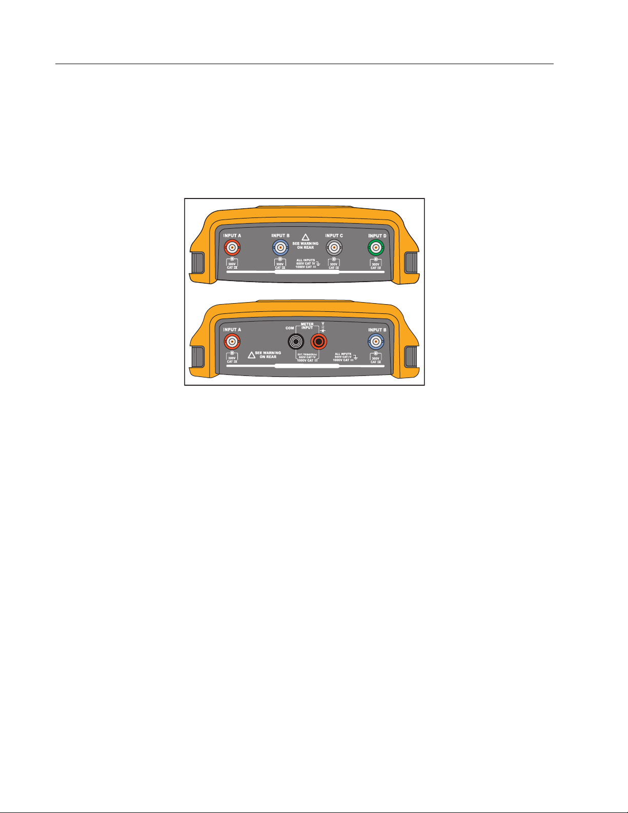
Input Connections

The top of the test tool has four safety BNC signal inputs (models 190–xx4/MDA-550) or two
safety BNC jack inputs and two safety 4-mm banana jack inputs (models 190-xx2). These
isolated inputs allow independent floating measurements with each input. The banana jack inputs
(190-xx2) can be used for DMM measurements or can be used as External Trigger input for the
Scope mode.

See Figure 3.

Figure 3. Measurement Connections

!

ALL INPUTS ISOLATED

!

ALL INPUTS ISOLATED

Note

To maximize the benefit of independent isolated floating inputs and to avoid problems
caused by improper use, see Tips.

For an accurate indication of the measured signal, you must match the probe to the input
channel on the test tool.

When using probes that are not included with the Product, see Voltage Probe Calibration.

Scope

To make scope measurements:

1. Connect the red voltage probe to input A, the blue voltage probe to input B, the gray voltage
probe to input C, and the green voltage probe to input D.

2. Connect the short ground leads of each voltage probe to its own reference potential. See

Figure 4.

10

Find Quality Products Online at: [e-mail]

www.GlobalTestSupply.com

ScopeMeter® Test Tool

How to Use the Test Tool

Figure 4. Scope Connections

XW Warning

To prevent electrical shock, use the insulation sleeve when you connect the
VPS410 Probe Set without the hook clip or the ground spring.

MDA Te st Too l

To make motor drive voltage and current measurements:

1. Connect the voltage probe to input A.

2. Connect the voltage probe tip to a phase.

3. For Phase-Phase measurements, connect the ground lead to another phase that is used as a

reference.

4. For Phase-Ground measurements, connect the ground lead to ground.

5. For the current measurement, place the clamp around one phase and connect the current

probe to input B.

After measurement selection, an on-screen connection diagram shows the connections for
each measurement.

To make motor drive 3-phase voltage unbalance measurements:

1. Connect the red voltage probe to input A, the blue voltage probe to input B, the gray voltage

probe to input C.

2. Connect the probe tip to a phase and the ground leads of each voltage probe to another

phase as shown in the connection diagram on the screen after you select the measurement.

3. For each phase, make sure that one probe tip and one ground lead are connected.

11

Find Quality Products Online at: [e-mail]

www.GlobalTestSupply.com

190 Series III

Users Manual

To make motor drive 3-phase current unbalance measurements:

1. Connect the current probes to the Inputs A, B and C.

2. Measure the current of each phase.

To make a motor shaft voltage measurement:

1. Connect the red VPS410-II voltage probe to the input A.

2. Connect the ground lead of the voltage probe to ground.

3. Connect a brush on top of the voltage probe.

4. Place the probe in probe holder.

5. Use the extension rod and magnetic base to keep the probe in a fixed position and the brush
in good contact with the motor shaft.

Probe Type Setup

To obtain correct measurement results the test tool probe type settings must correspond to the
connected probe types.

To select the input A probe setting:

1. Press A to show the INPUT A key labels.

2. Press 3 to open the PROBE ON A menu.

3. Use the cursor and E to select the probe type Voltage, Current, or Temp.

a. Voltage: select the voltage probe attenuation factor.

b. Current and Temp: select the current probe or temperature probe sensitivity.

12

Find Quality Products Online at: [e-mail]

www.GlobalTestSupply.com

Input Channel Selection

To select an input channel:

1. Press the required channel key (A-D):

• the channel is turned on

• the channel key illumination is turned on

ScopeMeter® Test Tool

How to Use the Test Tool

2. If the channel key is illuminated,

To set multiple channels to the same range (V/div) as, for example, input A, do the following:

1. Select the input A measurement function, probe setting and input options for all involved

channels.

2. Press and hold A.

3. Press B and/or C and/or D.

4. Release A.

Notice that all pressed keys are illuminated now.

L and K are now assigned to the indicated channel.

L and K applies to all involved input channels.

View an Unknown Signal with Connect-and-View™

The Connect-and-View™ feature lets the test tool show complex, unknown signals automatically.
This function optimizes the position, range, time base, and triggering and assures a stable
display of virtually any waveform. If the signal changes, the setup is automatically adjusted to
maintain the best display result. This feature is especially useful for quickly checking several
signals.

To enable the Connect-and-View feature when the test tool is in MANUAL mode:

1. Press

illumination is off.

The bottom line shows the range, the time base, and the trigger information. The waveform
identifier (A) is visible on the right side of the screen. See Figure 5. The input A zero icon - at
the left side of the screen identifies the ground level of the waveform.

2. Press

right of the screen, the key illumination is on.

Find Quality Products Online at: [e-mail]

J to perform an Auto Set. AUTO appears at the top right of the screen, the key

J a second time to select the manual range again. MANUAL appears at the top

13

www.GlobalTestSupply.com

190 Series III

Users Manual

Use

L K N V at the bottom of the keypad to change the view of the waveform

manually.

Figure 5. The Screen After an Auto Set

Automatic Scope Measurements

The test tool offers a wide range of automatic scope measurements. In addition to the waveforms
you can show four numeric readings: READING 1 - 4. These readings are selectable
independently, and the measurements can be done on the input A, input B, input C or input D
waveform.

To choose a Peak-Peak measurement for Input A, do the following:

1. Press

2. Open the READING menu with 2.

3. Select the reading number with 1, for example READING 1.

4. Use the cursor and E to select on A. Observe that the highlight jumps to the present
measurement.

5. Use the cursor and E to select the Hz measurement.

Observe that the top left of the screen shows the Hz measurement. See Figure 6.

To choose also a frequency measurement for Input B as second reading:

1. Press

2. Open the READING.. menu with 2.

P to show the SCOPE key labels.

P to show the SCOPE key labels.

3. Select the reading number with 1, for example READING 2.

4. Use the cursor and E to select on B. The highlight jumps to the measurements field.

5. Use the cursor and E to open the PEAK menu.

14

Find Quality Products Online at: [e-mail]

www.GlobalTestSupply.com

ScopeMeter® Test Tool

How to Use the Test Tool

6. Use the cursor and E to select the Peak-Peak measurement.

Figure 6 shows an example of the screen with two readings. The character size will be reduced

when more than two readings are on.

Figure 6. Hz and V peak-peak as Scope Readings

Freezing the Screen

You can freeze the screen (all readings and waveforms) at any time.

1. Press

illumination is on.

2. Press

H to freeze the screen. HOLD appears at the right of the reading area. The key

H again to resume your measurement. The key illumination is off.

Average, Persistence and Glitch Capture

Using Average for Smoothing Waveforms

To smooth the waveform:

1. Press

2. Open the WAVEFORM OPTIONS menu with 4.

3. Use

4. Use the cursor and E to select On... to open the AVERAGE menu.

5. Use the cursor and E to select Average factor: Average 64. This averages the

outcomes of 64 acquisitions.

P to show the SCOPE key labels.

g f to jump to Average:.

6. Use the cursor and E to select Average: Normal (normal average) or Smart (smart

average, see below).

You can use the average functions to suppress random or uncorrelated noise in the waveform
without loss of bandwidth. Waveform samples with and without smoothing are shown in Figure 7.

15

Find Quality Products Online at: [e-mail]

www.GlobalTestSupply.com

190 Series III

Users Manual

Smart Average

In the normal average mode occasional deviations in a waveform just distort the averaged wave
shape, and do not show up on screen clearly. When a signal really changes, for instance when
you probe around, it takes quite some time before the new wave shape is stable. With smart
averaging you can quickly probe around, and incidental waveform changes like a line flyback in
video show up on screen instantly.

Figure 7. Smoothing a Waveform

Persistence, Envelope and Dot-Join to View Waveforms

You can use Persistence to observe dynamic signals. See Figure 8.

1. Press

2. Open the WAVEFORM OPTIONS menu with 4.

3. Use the cursor and E to highlight to Waveform: and open the Persistence... menu.

4. Use the cursor and E to select:

a. Digital Persistence: Short, Medium, Long or Infinite to observe dynamic waveforms like on

b. Digital Persistence: Off, Display: Envelope to see the upper and lower boundaries of

c. Display Dot-join: Off to show measured samples only. Dot join off may be useful when

d. Display: Normal to turn the envelope mode off and the dot-join function on.

P to show the SCOPE key labels.

an analog oscilloscope.

dynamic waveforms (envelope mode).

measuring for example modulated signals or video signals.

16

Find Quality Products Online at: [e-mail]

www.GlobalTestSupply.com

Figure 8. Using Persistence to Observe Dynamic Signals

Glitch Display

To capture glitches on a waveform:

ScopeMeter® Test Tool

How to Use the Test Tool

1. Press

2. Open the WAVEFORM OPTIONS menu with 4.

3. Use the cursor and E to select Glitch: On.

4. Press 4 to exit the menu.

You can use this function to view events (glitches or other asynchronous waveforms) of 8 ns
(8 nanoseconds, due to ADCs with 125 MS/s sampling speed) or wider, or you can view HF
modulated waveforms.

By default, Glitch Detect is ON. Go to User Options to change the preference for the AUTO
mode.

When you select the 2 mV/div range Glitch Detect will automatically be turned Off. In the
2 mV/div range you can set Glitch Detect On manually.

P to show the SCOPE key labels.

17

Find Quality Products Online at: [e-mail]

www.GlobalTestSupply.com

190 Series III

Users Manual

High Frequency Noise Suppression

Switching the glitch detection off (Glitch: Off) will suppress the high frequency noise on a
waveform. Averaging will suppress the noise even more.

1. Press

2. Open the WAVEFORM OPTIONS menu with 4.

3. Use the cursor and E to select Glitch: Off, then select Average: On... to open the
AVERAGE menu.

4. Use the cursor and E to select Average 8.

See Using Average for Smoothing Waveforms.

Glitch capture and average do not affect bandwidth. Further noise suppression is possible with
bandwidth limiting filters. See Noisy Waveforms.

P to show the SCOPE key labels.

Waveform Acquisition

Set the Acquisition Speed and Waveform Memory Depth

To set the acquisition speed, do the following:

1. Press

2. Open the WAVEFORM OPTIONS menu with 4.

3. Use the cursor and E to select Acquisition:.

a. Fast - for fast waveform update rate; shortest record length, decreased zoom rate, no

P to show the SCOPE key labels.

readings possible.

b. Full - maximum waveform detail; 10 000 samples per waveform record length, maximum

zoom rate, lower waveform update rate.

c. Normal - optimal waveform update rate and zoom range combination.

4. Use 4 to exit the menu.

18

Find Quality Products Online at: [e-mail]

www.GlobalTestSupply.com

ScopeMeter® Test Tool

How to Use the Test Tool

AC-Coupling Selection

After a reset, the test tool is dc-coupled so that ac and dc voltages appear on the screen. Use ac­coupling when you wish to observe a small ac signal that rides on a dc signal.

To select ac-coupling, do the following:

1. Press A to show the INPUT A key labels.

2. Press 2 to highlight AC.

Observe that the bottom left of the screen shows the ac-coupling icon: .

You can define how Auto Set affects this setting, see Auto Set Options.

Reversing the Polarity of the Displayed Waveform

To invert, for example the input A waveform, do the following:

1. Press A to show the INPUT A key labels.

2. Press 4 to open the INPUT A menu.

3. Use the cursor and E to select Inverted and accept inverted waveform display.

4. Use 4 to exit the menu.

For example, a negative-going waveform is a positive-going waveform which may provide a more

meaningful view. An inverted display is identified by an inversed waveform identifier ( ) at the
right of the waveform, and in the status line below the waveform.

Variable Input Sensitivity

The variable input sensitivity allows you to adjust any input sensitivity continuously, for example
to set the amplitude of a reference signal to exactly 6 divisions. The input sensitivity of a range
can be increased up to 2.5 times, for example between 10 mV/div and 4 mV/div in the 10 mV/div
range.

To use the variable input sensitivity on for example input A, do the following:

1. Apply the input signal.

2. Press

An Auto Set will turn off the variable input sensitivity. You can now select the required input
range. Keep in mind that the sensitivity will increase when you start adjusting the variable
sensitivity (the displayed waveform amplitude will increase).

3. Press A to show the INPUT A key labels.

4. Press 4 to open the INPUT A menu.

J to Auto Set (AUTO shows at the top of the screen).

19

Find Quality Products Online at: [e-mail]

www.GlobalTestSupply.com

190 Series III

Users Manual

5. Use the cursor and E to select and accept Variable.

6. Use 4 to exit the menu.

A Var shows at the bottom left of the screen. Select Variable to turn off the cursors and
automatic input ranging.

7. Press

Variable input sensitivity is not available in the Mathematics functions (+ - x and
Spectrum).

j to increase the sensitivity and k to decrease the sensitivity.

Note

Noisy Waveforms

To suppress high frequency noise on waveforms, you can limit the working bandwidth to 10 kHz
or 20 MHz. This function smoothes the displayed waveform. For the same reason, it improves
triggering on the waveform.

To choose the 10 kHz bandwidth on for example input A, do the following:

1. Press A to show the INPUT A key labels.

2. Press 4 to open the INPUT A menu.

3. Use the cursor and E to highlight Bandwidth: and select 10kHz to accept the bandwidth
limitation.

Note

To suppress noise without loss of bandwidth, use the average function or turn off Display
Glitches.

Mathematic Functions +, -, x, XY-mode

You can add (+), subtract (-), or multiply (x) two waveforms. The test tool shows the mathematical
result waveform and the source waveforms. The XY-mode provides a plot with one input on the
vertical axis and the second input on the horizontal axis. The Mathematics functions perform a
point-to-point operation on the involved waveforms.

To use a Mathematics function, do the following:

1. Press

2. Open the WAVEFORM OPTIONS menu with 4.

20

P to show the SCOPE key labels.

Find Quality Products Online at: [e-mail]

www.GlobalTestSupply.com

3. Use the cursor and E to:

a. Highlight Waveform:

b. Select Mathematics... to open the Mathematics.

c. Select Function: +, -, x or XY-mode.

d. Select the first waveform: Source 1: A, B, C or D.

4. Select the second waveform: Source 2: A, B, C or D.

The mathematical function key labels show on the display.

5. Press:

ScopeMeter® Test Tool

How to Use the Test Tool

a. 2 -

b. 3 -

c. 4 - Toggle the result waveform between on or off.

The sensitivity range of the mathematical result is equal to the sensitivity range of the least
sensitive input divided by the scale factor.

h i
h i

to select a scale factor to fit the result waveform onto the display.

to move the result waveform up or down.

Mathematic Function Spectrum (FFT)

The Spectrum function shows the spectral content of the input A, B, C or D waveform in the input
waveform color. It performs an FFT (Fast Fourier Transform) to transform the amplitude
waveform from the time domain into the frequency domain. To reduce the effect of side-lobes
(leakage) it is recommended to use Auto windowing. This will automatically adapt the part of the
waveform that is analyzed to a complete number of cycles. Selecting Hanning, Hamming or no
windowing results in a faster update, but also in more leakage. Ensure that the entire waveform
amplitude remains on the screen.

To use the Spectrum function, do the following:

1. Press

2. Open the WAVEFORM OPTIONS menu with 4.

3. Use the cursor and E to:

P to show the SCOPE key labels.

a. Highlight Waveform:

b. Select Mathematics... to open the Mathematics.

c. Select Function: Spectrum.

d. Select Window: Auto (automatic windowing), Hanning, Hamming, or None (no

windowing).

21

Find Quality Products Online at: [e-mail]

www.GlobalTestSupply.com

190 Series III

Users Manual

Observe that the top right of the screen shows SPECTRUM. See Figure 9. If it shows LOW
AMPL a spectrum measurement cannot be done as the waveform amplitude is too low. If it
shows WRONG TB the time base setting does not enable the test tool to show an FFT result. It is
either too slow, which can result in aliasing, or too fast, which results in less than one signal
period on the screen.

4. Press 1 for spectrum analysis on waveform A, B, C or D.

5. Press 2 to set the horizontal amplitude scale to linear or logarithmic.

6. Press 3 to set the vertical amplitude scale to linear or logarithmic.

7. Press 4 to toggle the spectrum function between off or on.

Figure 9. Spectrum Measurement

Waveform Comparisons

You can display a fixed reference waveform with the actual waveform for visual comparison.

To create a reference waveform and to display it with the actual waveform, do the following:

1. Press

2. Open the WAVEFORM OPTIONS menu with 4.

3. Use the cursor and E to:

a. Highlight Waveform.

b. Select Reference to open the WAVEFORM REFERENCE menu.

P to show the SCOPE key labels.

22

Find Quality Products Online at: [e-mail]

www.GlobalTestSupply.com

ScopeMeter® Test Tool

black pixels: basic waveform
gray pixels: ±2 pixels envelope
1 vertical pixel on the display is 0.04 x range/div

1 horizontal pixel on the display is 0.04 x time/div.

How to Use the Test Tool

c. Select On to show the reference waveform.

This can be:

• last used reference waveform (if not available no reference waveform will be shown).

• envelope waveform if the persistence function Envelope is on.

d. Select Recall to recall a saved waveform (or waveform envelope) from memory and use it

as a reference waveform.

e. Select New to open the NEW REFERENCE menu.

If you selected New continue at step 4, if not, go to step 5.

4. Use

5. Press E to store the momentary waveform and show it permanently for reference. The

To recall a saved waveform from memory and use it as a reference waveform, see Recall

Screens with Associated Setups.

Example of reference waveform with an additional envelope of ±2 pixels:

h i

display also shows the actual waveform.

to select the width of an additional envelope to add to the momentary waveform.

Find Quality Products Online at: [e-mail]

www.GlobalTestSupply.com

23

190 Series III

Users Manual

Pass - Fail Tests

You can use a reference waveform as a test template for the actual waveform. If at least one
sample of a waveform is outside the test template, the failed or passed scope screen will be
stored. Up to 100 screens can be stored. If the memory is full, the first screen will be deleted in
favor of the new screen to be stored. The most appropriate reference waveform for the Pass-Fail
test is a waveform envelope.

To use the Pass - Fail function with a waveform envelope:

1. Show a reference waveform on the display. See Waveform Comparisons.

2. Use the cursor and E to:

a. Highlight Pass Fail Testing menu.

b. Select Store Fail saves each scope screen with samples outside the reference

c. Select Store Pass saves each scope screen with no samples outside the reference

Each time a scope screen is saved you will hear a beep. See Replay the 100 Most Recent Scope

Screens for information on how to analyze the saved screens.

Waveform Analysis

You can use the analysis functions CURSOR, ZOOM and REPLAY to perform detailed waveform
analysis. See Replay, Zoom and Cursors for more information.

Automatic Meter Measurements (190-xx4)

The test tool offers a wide range of automatic meter measurements. You can display four large
numeric readings: READING 1...4. These readings are selectable independently, and the
measurements can be done on the input A, B, C or input D waveform. In METER mode the
waveforms are not displayed. The 10 kHz HF rejection filter is always on in the METER mode.
See Noisy Waveforms

Meter Measurement Selection

To choose a current measurement for input A, do the following:

1. Press

2. Open the READING menu with 1.

3. Press 1 to select the reading number to be displayed, for example READING1.

M to show the METER key labels.

24

Find Quality Products Online at: [e-mail]

www.GlobalTestSupply.com

ScopeMeter® Test Tool

How to Use the Test Tool

4. Use the cursor and E to:

a. Select on A. Observe that the highlight jumps to the present measurement.

b. Select the A dc measurement.

c. Select a current probe sensitivity that matches the connected current probe. See Probe

Type Setup.

The display shows the screen in Figure 10.

Figure 10. Meter Screen

Note

To change the current probe sensitivity later, select another type of measurement (for
example, Vdc) and then select Amps again to see the sensitivity menu.

Relative Meter Measurements

A relative measurement displays the present measurement result relative to a defined reference
value. The following example shows how to perform a relative voltage measurement.

First obtain a reference value:

1. Press

2. Measure a voltage to use as a reference value.

3. Press 2 to set RELATIVE to ON. ON is highlighted.

This stores the reference value as reference for subsequent measurements. Observe the
ADJUST REFERENCE soft key (3) that enables you to adjust the reference value.

M to show the METER key labels.

25

Find Quality Products Online at: [e-mail]

www.GlobalTestSupply.com

190 Series III

Users Manual

4. Measure the voltage to be compared to the reference.

Now the large reading is the actual input value minus the stored reference value. The actual
input value is displayed below the large reading (ACTUAL: xxxx). See Figure 11. You can use
this feature when, for example, you need to monitor input activity (voltage, temperature) in
relation to a known good value.

Figure 11. Making a Relative Measurement

To adjust the reference value:

1. Press 3 to open the ADJUST REFERENCE menu.

2. Press 1 to select the applicable relative measurement reading.

3. Use

4. Use

5. Press E to use the new reference value.

g f to select the digit to adjust.

h i

to adjust the digit. Repeat until finished.

26

Find Quality Products Online at: [e-mail]

www.GlobalTestSupply.com

ScopeMeter® Test Tool

How to Use the Test Tool

Multimeter Measurements (190-xx2)

The screen displays the numeric readings of the measurements on the meter input.

Meter Connections

Use the two 4-mm safety red (VeG) and black (COM) banana jack inputs for the Meter
functions. See Figure 12.

Figure 12. Meter Connections

CAT II 1000V

CAT III 1000V
CAT IV 600V

Resistance Value Measurement

To measure a resistance:

1. Connect the red and black test leads from the 4-mm banana jack inputs to the resistor.

2. Press

3. Open the MEASUREMENT menu with 1.

4. Use cursor to highlight Ohms.

5. Press E to select Ohms measurement.

The resistor value shows on the display in Ohms. Observe that the bargraph shows as well.
See Figure 13.

M to show the METER key labels.

27

Find Quality Products Online at: [e-mail]

www.GlobalTestSupply.com

190 Series III

Users Manual

Figure 13. Resistor Value Readings

Current Measurement

You can measure current in both Scope mode and Meter mode. Scope mode has the advantage
of waveforms being displayed while you perform measurements. Meter mode has the advantage
of high measurement resolution.

The next example explains a typical current measurement in Meter mode.

XW Warning

Carefully read the instructions about the current probe you are using.

To set up the test tool:

1. Connect a current probe, for example, Fluke i410 (optional) between the 4-mm banana jack
inputs and the conductor to be measured.

2. Ensure that the red and black connectors correspond to the red and black banana jack inputs.
See Figure 14.

3. Press

M to show the METER key labels.

Figure 14. Measurement Setup

28

Find Quality Products Online at: [e-mail]

www.GlobalTestSupply.com

ScopeMeter® Test Tool

How to Use the Test Tool

4. Open the MEASUREMENT menu with 1.

5. Use the cursor to highlight A ac.

6. Press E to open the CURRENT PROBE submenu.

7. Observe the sensitivity of the current probe. Use the cursor to highlight the corresponding

sensitivity in the menu, for example, 1 mV/A.

Note

To change the current probe sensitivity later, select another type of measurement (for
example, Vdc) and then select Amps again to see the sensitivity menu.

8. Press E to accept the current measurement.

The display shows the screen in Figure 15.

Figure 15. Ampere Measurement Readings

Auto/Manual Range Selection

To activate manual ranging during any Meter measurement:

1. Press

2. Increase (V) or decrease (mV) the range with

Observe how the bar graph sensitivity changes. Use manual ranging to set a fixed bar graph
sensitivity and decimal point.

3. Press

When in auto ranging, the bar graph sensitivity and decimal point automatically adjust while
the test tool checks different signals.

J to activate manual ranging.

L.

J to choose auto ranging again.

29

Find Quality Products Online at: [e-mail]

www.GlobalTestSupply.com

190 Series III

Users Manual

Relative Meter Measurements

A relative measurement displays the present measurement result relative to a defined reference
value. You can use this feature to monitor input activity (voltage, temperature) in relation to a
known good value.

To make a relative voltage measurement:

1. Obtain a reference value.

2. Press

3. Measure a voltage to be used as the reference value.

4. Press 2 to set RELATIVE to ON. ON is highlighted.

This saves the reference value as reference for subsequent measurements. Observe the
ADJUST REFERENCE soft key (3) that enables you to adjust the reference value.

5. Measure the voltage to compare to the reference.

Now the large reading is the actual input value minus the stored reference value. The
bargraph indicates the actual input value. The actual input value and the reference value are
displayed below the large reading (ACTUAL: xxxx REFERENCE: xxx). See Figure 16.

M to show the METER key labels.

Figure 16. Making a Relative Measurement

To adjust the reference value:

1. Press 3 to open the ADJUST REFERENCE menu.

2. Use

3. Use

4. Press E to use the new reference value.

30

Find Quality Products Online at: [e-mail]

g f to select the digit to adjust.

h i

to adjust the digit. Repeat until finished.

www.GlobalTestSupply.com

ScopeMeter® Test Tool

Recorder Functions

Recorder Functions

This section provides a step-by-step introduction to the recorder functions of the test tool and
gives examples to show how to use the menus and perform basic operations.

Recorder Main Menu

First choose a measurement in scope or meter mode. Now you can choose the recorder
functions from the recorder main menu.

Press

Q to open the RECORDER menu.

Measurements Over Time (TrendPlot™)

Use the TrendPlot function to plot a graph of Scope or Meter measurements (readings) as
function of time. Trendplot Meter is only available with models 190-xx2.

Note

Because the navigation for the TrendPlot Scope and the TrendPlot Meter are identical,
only Scope TrendPlot is explained in this manual.

TrendPlot Function

To start a TrendPlot:

1. Make automatic Scope or Meter measurements, see Automatic Scope Measurements.

The readings plot on the display.

2. Press

3. Use

4. Press E to start the TrendPlot recording.

Q to open the RECORDER main menu.

h i

to highlight Trend Plot.

The test tool continuously records the digital readings of the measurements and displays
these as a graph. The TrendPlot graph rolls from right to left like a paper chart recorder.
Observe that the recorded time from start appears at the bottom of the screen. The present
reading appears at the top of the screen. See Figure 17.

5. Press 1 to set RECORDER to STOP to freeze the recorder function.

6. Press 1 to set RECORDER to RUN to restart.

Note

When simultaneously TrendPlotting two readings, the screen area is split into two
sections of four divisions each. When simultaneously TrendPlotting three or four
readings, the screen area is split into three or four sections of two divisions each.

31

Find Quality Products Online at: [e-mail]

www.GlobalTestSupply.com

190 Series III

Users Manual

Figure 17. TrendPlot Reading

When the test tool is in automatic mode, automatic vertical scaling is used to fit the TrendPlot
graph on the screen.

Note

Scope TrendPlot is not possible on cursor related measurements. As an alternative you
may use the PC software FlukeView™ ScopeMeter™.

Recorded Data Display

When in normal view (NORMAL), only the twelve most recently recorded divisions are displayed
on screen. All previous recordings are stored in memory.

VIEW ALL shows all data in memory:

1. Press 3 to show an overview of the full waveform.

2. Press 3 repeatedly to toggle between normal view (NORMAL) and overview (VIEW
ALL).

When the recorder memory is full, an automatic compression algorithm is used to compress all
samples into half of the memory without loss of transients. The other half of the recorder memory
is free again to continue recording.

Recorder Options

At the lower right of the display, the status line indicates a time. You can choose this time to
represent either the start time of the recording (Time of Day) or the time elapsed since the start of
the recording (From Start).

To change the time reference:

1. Press 2 to open the RECORDER OPTIONS menu.

2. Use the cursor and E to select Time of Day or From Start.

32

Find Quality Products Online at: [e-mail]

www.GlobalTestSupply.com

ScopeMeter® Test Tool

Recorder Functions

Turn Off the TrendPlot Display

Push 4 to exit the recorder function.

Recording Scope Waveforms In Deep Memory (Scope Record)

The SCOPE RECORD function is a roll mode that logs a long waveform of each active input. This
function can be used to monitor waveforms like motion control signals or the power-on event of
an Uninterruptable Power Supply (UPS). During recording, fast transients are captured. Because
of the deep memory, recording can be done for more than one day. This function is similar to the
roll mode in many DSOs but has deeper memory and better functionality.

Starting a Scope Record Function

To record, for example, the input A and input B waveform:

1. Apply a signal to input A and input B.

2. Press

3. Use the cursor and E to highlight Scope Record and start the recording.

The waveform moves across the screen from right to left like on a normal chart recorder. See

Figure 18.

Observe that the screen shows:

Q to open the RECORDER main menu.

Figure 18. Recording Waveforms

• Time from start at the top of the screen.

• The status at the bottom of the screen that includes the time/div setting as well as the total

timespan that fits the memory.

Note

For accurate recordings allow the test tool to warm up for a minimum of five minutes. For
long recordings, make sure the power supply is connected.

33

Find Quality Products Online at: [e-mail]

www.GlobalTestSupply.com

190 Series III

Users Manual

Recorded Data Display

In Normal view, the samples that roll off the screen are stored in deep memory. When the
memory is full, recording continues by shifting the data in memory and deleting the first samples
out of memory.

In View All mode, the complete memory contents are displayed on the screen. Press 3 to
toggle between VIEW ALL (overview of all recorded samples) and NORMAL view.

You can analyze the recorded waveforms using the Cursors and Zoom functions. See Replay,

Zoom and Cursors.

Scope Record in Single Sweep Mode

Use the recorder Single Sweep function to automatically stop recording when the deep memory
is full.

To s et u p:

1. Start the record mode. See Starting a Scope Record Function.

2. Press 1 to stop recording and unlock the OPTIONS softkey.

3. Press 2 to open the RECORDER OPTIONS menu.

4. Use the cursor and E to highlight the Mode field, select Single Sweep, and accept the
recorder options.

5. Press 1 to start recording.

Triggering to Start or Stop Scope Record

To record an electrical event that causes a fault, it might be useful to start or stop recording on a
trigger signal: Start on trigger to start recording; recording stops when the deep memory is full
Stop on trigger to stop recording. Stop when untriggered to continue recording as long as a next
trigger comes within 1 division in view all mode.

• For the models 190-xx4 the signal on the BNC input that has been selected as trigger source
must cause the trigger.

• For the models 190-xx2 the signal applied to the banana jack inputs (EXT TRIGGER (in)).
signal must cause the trigger. The trigger source is automatically set to Ext. (external).

To s et u p:

1. Start the record mode. See Starting a Scope Record Function.

2. Apply the signal to be recorded to the BNC input(s).

3. Press 1 to stop recording and unlock the OPTIONS softkey.

34

Find Quality Products Online at: [e-mail]

www.GlobalTestSupply.com

ScopeMeter® Test Tool

Recorder Functions

4. Press 2 to open the RECORDER OPTIONS menu.

5. Use the cursor and E to highlight the Mode field and select:

a. on Trigger (190-xx4) opens the START SINGLE SWEEP ON TRIGGERING menu

b. on Ext. (190-xx2) opens the START SINGLE SWEEP ON EXT. menu

6. Use the cursor and E to select one of the Conditions: and accept the selection.

For external triggering (190-xx2) continue with:

7. Use the cursor and E to select the trigger slope (Slope) and level (Level).

8. Use the cursor and E to select the 0.12V or 1.2V trigger level and accept all recorder

options.

9. Apply a trigger signal to the red and black ext. trigger banana inputs.

During recording samples are continuously saved in deep memory. The last twelve recorded
divisions show on the screen. See Figure 19. Use View All to display the full memory contents.

Note

To learn more about the Single Shot trigger function, see Waveform Triggers.

Figure 19. Triggered Single Sweep Recording

TrendPlot or Scope Record Analysis

From a TrendPlot or Scope Record you can use the analysis functions CURSORS and ZOOM to
perform detailed waveform analysis. See Replay, Zoom and Cursors.

35

Find Quality Products Online at: [e-mail]

www.GlobalTestSupply.com

190 Series III

Users Manual

Replay, Zoom and Cursors

This section covers the capabilities of the analysis functions Cursor, Zoom, and Replay. These
functions can be used with one or more of the primary functions Scope, TrendPlot or Scope
Record. It is possible to combine two or three analysis functions.

A typical application uses these functions:

• replay the last screens to find the screen of special interest

• zoom in on the signal event

• make measurements with the cursors.

Replay the 100 Most Recent Scope Screens

When you are in Scope mode, the test tool automatically stores the 100 most recent screens.
When you press the HOLD key or the REPLAY key, the memory contents are frozen. Use the
functions in the REPLAY menu to go back in time by stepping through the stored screens to find
the screen of your interest. This feature lets you capture and view signals even if you did not
press HOLD.

Replay Step-by-Step

To step through the last scope screens:

1. From Scope mode, press

Observe that the waveform is frozen and that REPLAY appears at the top of the screen. See

Figure 20.

2. Press 1 to step through the previous screens.

3. Press 2 to step through the next screens.

Observe that the bottom of the waveform area displays the replay bar with a screen number
and related time stamp.

R open the REPLAY menu.

36

Find Quality Products Online at: [e-mail]

www.GlobalTestSupply.com

ScopeMeter® Test Tool

Replay, Zoom and Cursors

Figure 20. Replaying a Waveform

The replay bar represents all 100 stored screens in memory. The icon represents the picture
being displayed on the screen (in this example: SCREEN -52). If the bar is partly white, the
memory is not completely filled with 100 screens.

From this point you can use the zoom and cursor functions to study the signal in more detail.

Replay Continuously

You can also continuously replay the stored screens as a video.

To replay continuously:

1. From Scope mode, press

Observe that the waveform is frozen and REPLAY appears at the top of the screen.

2. Press 3 to continuously replay the stored screens in ascending order.

Wait until the screen with the signal event of interest appears.

3. Press 3 to stop the continuous replay.

R open the REPLAY menu.

Turn Off the Replay Function

Press 4 to turn off REPLAY.

Capturing 100 Intermittent Signals Automatically

When you use the test tool in triggered mode, 100 triggered screens are captured. By combining
the trigger possibilities with the capability of capturing 100 screens for later replay, you can leave
the test tool unattended to capture intermittent signal anomalies. This way you could use Pulse
Triggering to trigger and capture 100 intermittent glitches or you could capture 100 UPS startups.

For triggering, see Waveform Triggers.

37

Find Quality Products Online at: [e-mail]

www.GlobalTestSupply.com

190 Series III

Users Manual

Zoom on a Waveform

To obtain a more detailed view of a waveform, you can zoom in on a waveform using the ZOOM
function.

To zoom in on a waveform:

1. Press

ZOOM shows at the top of the screen and the waveform is magnified.

2. Use

waveform.

3. Use
total waveform.

Even when the key labels are not displayed at the bottom of the screen, you can still use
the arrow keys to zoom in and out. You can also use the s TIME ns key to zoom in and
out.

Observe that the bottom of the waveform area displays the zoom ratio, position bar, and time/
div See Figure 21. The zoom range depends on the amount of data samples stored in
memory.

Z to show the ZOOM key labels.

h i

to enlarge (decrease the time/div) or shrink (increase the time/div) the

g f to scroll. A position bar displays the position of the zoomed part in relation to the

Note

Figure 21. Zoom on a Waveform

4. Push 4 to turn off the ZOOM function.

38

Find Quality Products Online at: [e-mail]

www.GlobalTestSupply.com

ScopeMeter® Test Tool

Replay, Zoom and Cursors

Cursor Measurements

Cursors allow you to make precise digital measurements on waveforms. This can be done on live
waveforms, recorded waveforms, and on saved waveforms.

Horizontal Cursors on a Waveform

To use the cursors for a voltage measurement:

1. From Scope mode, press

2. Press 1 to highlight the horizontal cursor icon.

3. Press 2 to highlight the upper cursor icon.

4. Use

5. Press 2 to highlight the lower cursor.

6. Use

The screen shows the voltage difference between the two cursors and the voltage at the cursors.
See Figure 22. Use horizontal cursors to measure the amplitude, high or low value, or overshoot
of a waveform.

h i

h i

Even when the key labels are not displayed at the bottom of the screen, you can use the
cursor. This allows full control of both cursors while having full screen view.

to move the upper cursor position on the screen.

to move the lower cursor position on the screen.

Figure 22. Voltage Measurement with Cursors

G to show the cursor key labels.

Note

39

Find Quality Products Online at: [e-mail]

www.GlobalTestSupply.com

190 Series III

Users Manual

Vertical Cursors on a Waveform

To use the cursors for a time measurement (T, 1/T), for a mVs-mAs-mWs measurement, or for an
RMS measurement of the waveform section between the cursors:

1. From Scope mode, press

2. Press 1 to highlight the vertical cursor icon.

3. Press 3 to choose, for example, time measurement: T.

4. Press 4 to choose the waveform to place the markers: A, B, C, D or M (Mathematics).

5. Press 2 to highlight the left cursor icon.

6. Use

7. Press 2 to highlight the right cursor.

8. Use

g f to move the left cursor position on the waveform.

g f to move the right cursor position on the waveform.

The screen shows the time difference between the cursors and the voltage difference
between the two markers. See Figure 23.

G to show the cursor key labels.

Figure 23. Time Measurement with Cursors

9. Press 4 to select OFF and turn off the cursors.

Note

For an mVs-mAs-mWs measurement:

- mVs: select probe type as Voltage

- mAs: select probe type as Current

- mWs: select the mathematical function as x, probe type as Voltage for one channel, and

Current for the other channel

40

Find Quality Products Online at: [e-mail]

www.GlobalTestSupply.com

ScopeMeter® Test Tool

Replay, Zoom and Cursors

Cursors on a Mathematical Result (+ - x) Waveform

Cursor measurements on, for example, an AxB waveform give a reading in Watts if input A
measures (milli)Volts and input B measures (milli)Amperes. For other cursor measurements on,
for example, a A+B, A-B or AxB waveform no reading will be available if the input A and input B
measurement unit are different.

Cursors on Spectrum Measurements

For a cursor measurent on a spectrum:

1. From the Spectrum measurement screen, press

2. Use

g f to move the cursor and observe the readings at the top of the screen.

G to show the cursor key label.

Rise Time Measurements

For rise time measurements:

1. From Scope mode, press

2. Press 1 to highlight the Rise time icon.

3. For multiple waveforms, press 4 to select the required waveform A, B, C, D or M (if a

math function is active).

4. Press 3 to select MANUAL or AUTO (this automatically does steps 5 to 7).

5. Use

6. Press 2 to highlight the Fall time icon.

h i

A marker is shown at 90 %.

to move the upper cursor to 100 % of the waveform height.

G to show the cursor key labels.

41

Find Quality Products Online at: [e-mail]

www.GlobalTestSupply.com

190 Series III

Users Manual

7. Use

h i

A marker is shown at 10 %.

The reading shows the rise time from 10 % to 90 % of the waveform amplitude. See

Figure 24.

to move the lower cursor to 0 % of the waveform height.

Figure 24. Risetime Measurement

Note

Direct access to Rise time or Fall time with cursors on is possible with the key sequence
SCOPE, 2 (READING), and then selection of Rise or Fall time.

42

Find Quality Products Online at: [e-mail]

www.GlobalTestSupply.com

ScopeMeter® Test Tool

Waveform Triggers

Waveform Triggers

This section provides an introduction to the trigger functions of the test tool. Triggering tells the
test tool when to begin displaying the waveform. You can use fully automatic triggering, take
control of one or more main trigger functions (semi-automatic triggering), or you can use
dedicated trigger functions to capture special waveforms.

Typical trigger applications:

• Use the Connect-and-View function to have full automatic triggering and instant display of

virtually any waveform.

• If the signal is unstable or has a very low frequency, you can control the trigger level, slope,

and trigger delay for a better view of the signal. (See next section.)

For dedicated applications, use one of the manual trigger functions:

• Edge triggering

• Pulse Width triggering

• External Triggering (models 190-xx2 only)

Trigger Level and Slope

The Connect-and-View™ function enables hands-off triggering to display complex unknown
signals.

When the test tool is in manual range:

1. Press

AUTO appears at the top right of the screen.

Automatic triggering assures a stable display of virtually any signal.

From this point, you can take over the basic trigger controls such as level, slope and delay. To
optimize trigger level and slope manually:

2. Press

3. Press 2 to trigger on either positive slope or negative slope of the chosen waveform.

In Dual Slope Triggering (X) the test tool triggers on both positive slope and negative slope.

4. Press 3 to enable the cursor for manual trigger level adjustment.

5. Use

Observe that the trigger icon indicates the trigger position, trigger level, and slope.

J to do an auto set.

T to show the TRIGGER key labels.

h i

to adjust the trigger level.

43

Find Quality Products Online at: [e-mail]

www.GlobalTestSupply.com

190 Series III

Users Manual

At the bottom of the screen the trigger parameters show. See Figure 25. For example, input A is
used as the trigger source with a positive slope.

Figure 25. Screen with all Trigger Information

When a valid trigger signal is found, the trigger key will be lit and the trigger parameters appear in
black. When no trigger is found, the trigger parameters appear in gray and the key light will be
off.

Trigger Delay or Pre-Trigger

You can begin to display the waveform some time before or after the trigger point has been
detected. Initially, you have a half screen (6 divisions) of pre-trigger view (negative delay).

To set the trigger delay:

1. Press and hold down

Observe that the trigger icon on the screen moves to show the new trigger position. When the
trigger position moves left off of the screen, the trigger icon changes to indicate that you have
selected a trigger delay. Moving the trigger icon to the right on the display gives you a pre-trigger
view. This allows you to see what happened before the trigger event, or what caused the trigger.

In case of a trigger delay, the status at the bottom of the screen changes. See Figure 26. For
example, input A is used as the trigger source with a positive slope. The 500.0 ms indicates the
(positive) delay between trigger point and waveform display. When a valid trigger signal is found,
the trigger key will be lit and the trigger parameters appear in black. When no trigger is found, the
trigger parameters appear in gray, ands the key light will be off.

N to adjust the trigger delay.

44

Find Quality Products Online at: [e-mail]

www.GlobalTestSupply.com

ScopeMeter® Test Tool

Waveform Triggers

Figure 26 shows an example of a trigger delay of 500 ms (top) and an example of pre-trigger

view of 8 divisions (bottom).

Figure 26. Trigger Delay or Pre-Trigger View

Automatic Trigger Options

The Trigger Menu has the settings for automatic triggering.

To change:

1. Press

The TRIGGER key labels can differ depending on the latest trigger function used.

2. Press 4 to open the TRIGGER OPTIONS menu.

3. Use the cursor and E to open the AUTOMATIC TRIGGER menu.

If the frequency range of the automatic triggering is set to >15 Hz, the Connect-and-View
function responds more quickly. The response is quicker because the test tool is instructed
not to analyze low frequency signal components. However, when you measure frequencies
lower than 15 Hz, the test tool must be instructed to analyze low frequency components for
automatic triggering.

4. Use the cursor and E to select >1 Hz and return to the measurement screen.

See also View an Unknown Signal with Connect-and-View™.

T to show the TRIGGER key labels.

Note

45

Find Quality Products Online at: [e-mail]

www.GlobalTestSupply.com

190 Series III

Users Manual

Edge Triggers

If the signal is unstable or has a very low frequency, use edge triggering to obtain full manual
trigger control.

To trigger on rising edges of the input A waveform:

1. Press

2. Press 4 to open the TRIGGER OPTIONS menu.

3. Use the cursor and E to open the TRIGGER ON EDGE menu.

When Free Run is selected, the test tool updates the screen even if there are no triggers. A
waveform always appears on the screen.

When On Trigger is selected, the test tool needs a trigger to display a waveform. Use this
mode if you want to update the screen only when valid triggers occur.

When Single Shot is selected, the test tool waits for a trigger. After receiving a trigger, the
waveform is displayed and the instrument is set to HOLD.

In most cases, use the Free Run mode.

4. Use the cursor and E to select Free Run, jump to Trigger Filter.

5. Use the cursor and E to set Trigger Filter to Off.

Observe that the key labels at the bottom of the screen have adapted to allow further
selection of specific edge trigger settings.

T to show the TRIGGER key labels.

Noisy Waveform Triggers

To reduce jitter on the screen when triggering on noisy waveforms, you can use a trigger filter.

Continue from step 3 of the previous example:

1. Use the cursor and E to select On Trigger and jump to Trigger Filter.

2. Use the cursor and E to set Noise Reject or HF Reject to On. This is indicated by a
taller trigger icon.

When Noise Reject is on, an increased trigger gap is applied. When HF Reject is on, HF
noise on the (internal) trigger signal is suppressed.

46

Find Quality Products Online at: [e-mail]

www.GlobalTestSupply.com

ScopeMeter® Test Tool

Waveform Triggers

Single Event Acquisition

To catch single events, you can perform a single shot acquisition (one-time screen update). To
set up the test tool for a single shot of the input A waveform, continue from step 3 again:

1. Use the cursor and E to select Single Shot.

The word MANUAL appears at the top of the screen indicating that the test tool is waiting for
a trigger. As soon as the test tool receives a trigger, the waveform is displayed and the
instrument is set to hold. This is indicated by the word HOLD at top of the screen. See

Figure 27.

2. Press

The test tool stores all single shots in the replay memory. Use the Replay function to look
at all the stored single shots. See Replay, Zoom and Cursors.

H to arm the test tool for a new single shot.

Note

Figure 27. Making a Single Shot Measurement

N-Cycle Trigger

N-Cycle triggering enables you to create a stable picture of for example n-cycle burst waveforms.
Each next trigger is generated after the waveform has crossed the trigger level N times in the
direction that complies with the selected trigger slope.

To select N-Cycle triggering, continue from step 3 again:

1. Use the cursor and E to select On Trigger or Single Shot, jump to Trigger Filter.

47

Find Quality Products Online at: [e-mail]

www.GlobalTestSupply.com

190 Series III

Users Manual

2. Use the cursor and E to select a Trigger Filter or set it Off.

3. Use the cursor and E to set NCycle to On.

Observe that the key labels at the bottom of the screen have been changed to allow further
selection of specific N-Cycle trigger settings.

4. Use

5. Use

g f to set the number of cycles N.

h i

Waveforms with N-Cycle trigger (N=7) show on the display. See Figure 28.

to adjust the trigger level.

Figure 28. Waveforms with N-Cycle Trigger

External Waveform Triggers (190-xx2)

Use external triggering when you want to display waveforms on inputs A and B while triggering
on a third signal.

You can choose external triggering with automatic triggering or with edge triggering:

1. Supply a signal to the red and black 4-mm banana jack inputs.

In this example you continue from the Trigger on Edges example.

To choose the external signal as trigger source:

2. Press

3. Press 1 to select Ext (external) edge trigger.

Observe that the key labels at the bottom of the screen have been adapted to allow selection
of two different external trigger levels: 0.12 V and 1.2 V.

4. Press 3 to select 1.2V under the Ext LEVEL label.

From this point the trigger level is fixed and is compatible with logic signals.

48

T to show the TRIGGER (On Edges) key labels.

Find Quality Products Online at: [e-mail]

www.GlobalTestSupply.com

ScopeMeter® Test Tool

Waveform Triggers

Pulse Triggers

Use pulse width triggering to isolate and display specific pulses that you can qualify by time, such
as glitches, missing pulses, bursts or signal dropouts.

Narrow Pulses

To set the test tool to trigger on narrow positive pulses shorter than 5 ms:

1. Apply a video signal to the red input A.

2. Press

3. Press 4 to open the TRIGGER OPTIONS menu.

4. Use the cursor and E select Pulse Width on A to open the trigger on pulse width menu.

5. Use the cursor and E to select the negative pulse icon and jump to Condition.

6. Use the cursor and E to select <t and jump to Update.

7. Use the cursor and E to select On Trigger.

The test tool is now prepared to trigger on narrow pulses only. Observe that the trigger key
labels at the bottom of the screen have been adapted to set the pulse conditions.

To set the pulse width to 100 μs:

8. Press 1 to enable the cursor to adjust the pulse width.

9. Use

All narrow positive pulses less than 100 μs show on the screen. See Figure 29.

The test tool stores all triggered screens in the replay memory. For example, if you setup
the trigger for glitches, you can capture 100 glitches with time stamps. Use the REPLAY
key to look at all the stored glitches.

T to show the TRIGGER key labels.

h i

to select 100 μs.

Note

Figure 29. Trigger on Narrow Glitches

49

Find Quality Products Online at: [e-mail]

www.GlobalTestSupply.com

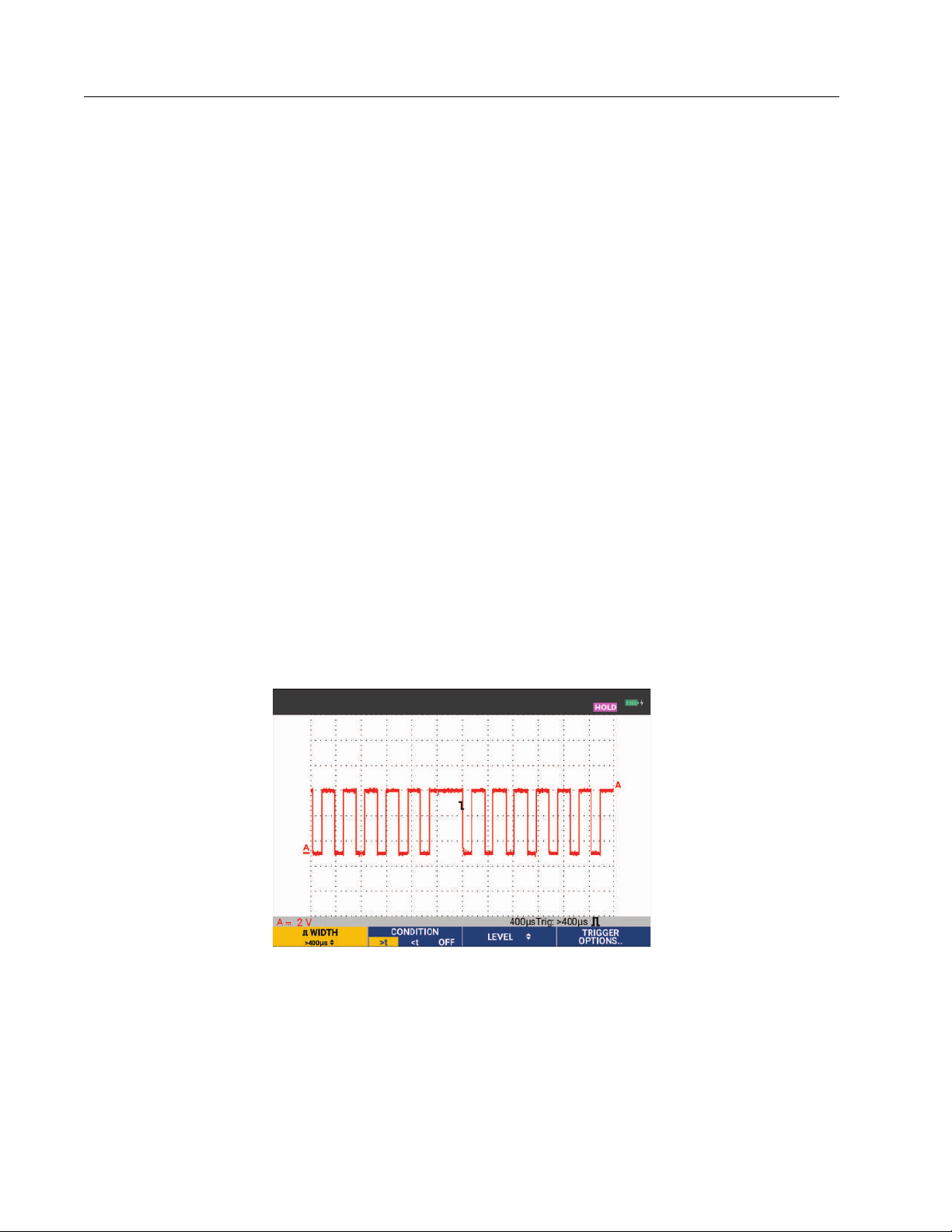
190 Series III

Users Manual

Missing Pulses

The next example is about how to find missing pulses in a train of positive pulses. In this
example, it is assumed that the pulses have a 100 ms distance between the rising edges. If the
time accidentally increases to 200 ms, a pulse is missing.

To set the test tool to trigger on such missing pulses, let it trigger on gaps bigger than 110 ms:

1. Press

2. Press 4 to open the TRIGGER OPTIONS menu.

3. Use the cursor and E to select Pulse Width on A and open the TRIGGER ON PULSE
WIDTH menu.

4. Use the cursor and E to select the positive pulse icon to trigger on a positive pulse, then
jump to Condition.

5. Use the cursor and E to select >t and jump to Update.

6. Use the cursor and E to select On Trigger and exit the menu.

The test tool is now prepared to trigger on pulses that are more than a selectable time in
duration. Observe that the trigger menu at the bottom of the screen has been adapted to set the
pulse condition. See Figure 30.

To set the pulse width to 400 μs:

7. Press 1 to enable the cursor and adjust the pulse width.

8. Use

T to show the TRIGGER key labels.

h i

to select 400 μs.

Figure 30. Trigger on Missing Pulses

50

Find Quality Products Online at: [e-mail]

www.GlobalTestSupply.com

ScopeMeter® Test Tool

Memory and PC

Memory and PC

This section provides a step-by-step introduction to the general functions of the test tool that can
be used in the three main modes: Scope, Meter, or Recorder. You will find information on
computer communication at the end of this section.

USB Ports

The test tool is provided with two USB ports:

• USB-host port to connect an external flash memory drive (USB-stick) for data storage. The

maximum memory size is 32 GB.

• Mini-USB-B port to connect the test tool to a PC for remote control and data transfer under

PC-control, see FlukeView™ 2 Software.

The USB port is also used with the optional WiFi-USB Adapter as a wireless connection to a PC
that has FlukeView 2 software installed. See WiFi Connection.

The ports are fully isolated from the input channels and have a dust cover when not in use. See

Figure 31.

Figure 31. Test Tool USB Connections

51

Find Quality Products Online at: [e-mail]

www.GlobalTestSupply.com

190 Series III

Users Manual

USB Drivers

To communicate, the test tool requires USB driver installation on your computer. Windows 10 and
later automatically recognizes the test tool and uses the drivers supplied by Windows. No special
drivers are required. Windows activates these drivers the first time you connect the test tool. An
admin account and active Internet connection may be required to allow Windows to load the
latest drivers.

After you install the drivers, an additional USB Composite Device shows in the Windows Device
Manager, Universal Serial Bus Controllers section. At this point, you are ready to use
FlukeView 2 software through the USB connection.

Next to the USB device is also a USB Serial Device (COM 3) that shows in the Windows Device

Manager Ports section. This Com port is for calibration purpose.

Note

The COM port number may differ and is automatically assigned by Windows.

Save and Recall

The test tool can:

• Save screens and setups to internal memory, and recall them again from memory. The test
tool has 30 screen and setup memories, 10 record and setup memories, and 9 screen image
memories. See Tab le 4 .

• Save up to 256 screens and setups to a USB memory device, and recall them again from
memory.

• Name saved screens and setups according to your own preferences.

• Recall screens and recordings to analyze the screen image at a later date.

• Recall a setup to continue a measurement with the recalled operating configuration.

Saved data is stored in non-volatile Flash memory. Not saved instrument data is stored in RAM
memory and will be kept at least 30 seconds when the battery is removed when no power is
supplied via the BC190 power adapter.

Table 4. Test Tool Internal Memory

Mode

30x 10x 9x

Meter Setup + 1 screen --- Screen image

Scope Setup + 1 screen Setup + 100 replay screens Screen image

Memory Locations

Scope Recorder --- Setup + record data Screen image

TrendPlot --- Setup+ TrendPlot data Screen image

52

Find Quality Products Online at: [e-mail]

www.GlobalTestSupply.com

ScopeMeter® Test Tool

Memory and PC

In persistence mode, the most recent waveform will be saved, not all waveforms that build the
persistence display.

The file list of stored data uses these icons:

• setup + 1 screen

• setup + replay screens/record data

• setup + trendplot data

• screen image (imagexxx.bmp)

You can copy a screen image to a USB stick connected to the test tool. The USB stick connected
to a PC allows you to insert the image, for example, into a text document. The copying function is
available under SAVE and File OPTIONS. A screen image can not be recalled on to the screen.

Save Screens with Associated Setups

To save, for example a screen + setup, in Scope mode:

1. Press

From this point the screen is frozen.

2. Press 1 to open the SAVE menu.

Observe the number of available and used memory locations.

In METER mode the SAVE AS menu shows as only a setup+screen to save, see step 4.

3. Press 1 to select the target memory INT (internal memory) or USB (USB device).

Observe the new SAVE menu if you select USB.

You can save data in .csv format to a USB stick. The saved .csv file can be used to analyze
the data in, for example, FlukeView ScopeMeter or in Excel.

4. Use the cursor and E to select Screen+Setup and open the SAVE AS menu.

Below Save As, the default name + serial number and OK SAVE are selected. To modify the
name for this particular Screen+Setup or to modify the default name, see Editing Names.

5. Press E to save the Screen+Setup.

6. To resume measurements, press

S to show the SAVE key labels.

H.

53

Find Quality Products Online at: [e-mail]

www.GlobalTestSupply.com

190 Series III

Users Manual

All Memories in Use

If no free memory locations are available a message pops up that proposes to you to overwrite
the oldest data set:

• If you do not want to overwrite the oldest data set, press 3. Delete one or more
memory locations and save again.

• If you want to overwrite the oldest data set, press 4.

Editing Names

To name the Screen+Setup according to your own preferences, continue from step 4 in Save

Screens with Associated Setups:

5. Press 1 to open the EDIT NAME menu.

6. Press 2 to skip to a new character position.

7. Use the cursor and E to select another character and press ENTER to accept your
choice. Continue to edit characters until you are done.

8. Press 1 to accept the name and return to the SAVE AS menu.

9. Use the cursor and E to highlight OK SAVE to save the actual screen with the edited
name.

To modify the default name generated by the test tool, continue from SAVE AS menu in step 8:

9. Use the cursor and E to highlight SET DEFAULT and save the new default name.

10. Use the cursor and E to highlight OK SAVE and save the actual screen using the new
default name.

The Record+Setup memory locations store more than what is visible on the screen. In TrendPlot
or Scope Record mode, the full recording is saved. In Scope mode you can save all 100 replay
screens in a single Record+Setup memory location.

To save a TrendPlot select STOP first.

Save Screens in .bmp Format (Print Screen)

To save a screen in bitmap (.bmp) format:

1. Press

2. Press 3 to save the screen to:

• Internal memory (INT) if no USB device is connected.

• USB device if connected.

S to show the SAVE key labels.

54

Find Quality Products Online at: [e-mail]

www.GlobalTestSupply.com

ScopeMeter® Test Tool

Memory and PC

The file is saved using a fixed name (IMAGE) and a serial number, for example IMAGE004.bmp.
If no free memory locations are available a message pops up that proposes to you to overwrite
the oldest data set:

• If you do not want to overwrite the oldest data set, press 3, then delete one or more

memory locations, and save again.

• If you want to overwrite the oldest data set, press 4.

Delete Screens with Associated Setups

To delete a screen and associated setup:

1. Press

2. Press 4 to open the FILE OPTIONS menu.

3. Press 1 to select the source as internal memory (INT) or a USB device.

4. Use

5. Press E to accept the choice and jump to the filename field.

6. Use

7. Press E to delete the selected files.

S to show the SAVE key labels.

h i

h i

to highlight DELETE.

to select the file to be deleted or 2 to select all files for deletion.

Recall Screens with Associated Setups

To recall a Screen+Setup:

1. Press

2. Press 2 to open the RECALL menu.

3. Press 1 to select the source as internal memory (INT) or a USB device.

4. Use

5. Press E to accept your choice and jump to the filename field.

6. Use

S to show the SAVE key labels.

h i

h i

to highlight DATA.

to select the file to be recalled.

7. Press E to recall the selected Screen+Setup.

Observe that the recalled waveform is on the display and that HOLD appears on the screen.
From this point you can use cursors and zoom for analysis or you can print the recalled
screen.

To recall a screen as a reference waveform to compare it to an actually measured waveform, see

Waveform Comparisons.

55

Find Quality Products Online at: [e-mail]

www.GlobalTestSupply.com

190 Series III

Users Manual

Recall a Setup Configuration

To recall a setup configuration:

1. Press

2. Press 2 to open the RECALL menu.

3. Press 1 to select the source as internal memory (INT) or a USB device.

4. Use

5. Press E to accept your choice and jump to the filename field.

6. Use

7. Press E to recall the selected setup.

From this point you continue in the new operating configuration.

S to show the SAVE key labels.

h i

h i

to highlight Setup.

to select the file to be recalled.

View Stored Screens

To scroll through the memories while looking at the stored screens:

1. Press

2. Press 2 to open the RECALL menu.

3. Press 1 to select the source as internal memory (INT) or a USB device.

4. Press E to jump to the filename field.

5. Use

6. Press 2 to view the screen and open the viewer.

S to show the SAVE key labels.

h i

to highlight a file.

7. Use

8. Press 3 to save the screen to USB device (if connected) or internal memory.

9. Press 4 to exit the View mode.

56

h i

You cannot view the replay screens of a saved Record+Setup in VIEW mode. Only the
screen at the Save instant can be reviewed with this method. To see all replay screens,
recall them from memory with the RECALL option.

to scroll through all stored screens.

Note

Find Quality Products Online at: [e-mail]

www.GlobalTestSupply.com

Rename Stored Screens and Setup Files

To modify the name of stored files:

ScopeMeter® Test Tool

Memory and PC

1. Press

2. Press 4 to open the FILE OPTIONS menu.

3. Press 1 to select the source as internal memory (INT).

4. Use

5. Press E to accept your choice and jump to the filename field.

6. Use

7. Press E to open the RENAME menu.

8. Press 2 to jump to a new character position.

9. Use the cursor and E to select another character. Repeat 8 and 9 until done.

10. Press 1 to accept the name and return to the RENAME menu.

S to show the SAVE key labels.

h i

h i

to highlight RENAME.

to highlight the file to be renamed.

Copy/Move Stored Screens and Setup Files

You can copy or move a file from internal memory to a USB device or from a USB device to
internal memory.

To copy or to move a file:

1. Press

S to show the SAVE key labels.

2. Press 4 to open the FILE OPTIONS menu.

3. Press 1 to select the source as internal memory (INT) or a USB device. The other

memory is the destination.

4. Use

5. Press E to accept your choice and jump to the filename field.

6. Use

7. Use

h i

h i
h i

to highlight COPY or MOVE (copy and delete source) a file.

to select the file to be copied or moved or 2 to SELECT ALL FILES.

to copy or delete the selected files.

57

Find Quality Products Online at: [e-mail]

www.GlobalTestSupply.com

190 Series III

Users Manual

FlukeView™ 2 Software

With the FlukeView 2 software you can upload waveform data and screen bitmaps to your PC or
notebook computer for further processing.

Af

ter installation:

1. Start the FlukeView 2 software.

2. Push HELP to access the documentation for the program.

Computer Connection

To connect the test tool to a PC or notebook computer and use the FlukeView 2 software for

®

Windows

1. Use a USB-A to mini-USB-B interface cable to connect a computer to the mini USB PORT of
the test tool. See Figure 32.

The USB drivers automatically install. See USB Drivers.

:

2. Install the FlukeView 2 Demo version. For information about how to install and use the
software see the FlukeView 2 Users Manual.

The optional kit SCC293 contains an activation code to convert the FlukeView 2 Demo version
into a fully operational version. You can order the complete FlukeView 2 version with ordering
code FlukeView 2.

The test tool input channels are electrically isolated from the USB port. Remote control and data
transfer through the mini-USB port is not possible while saving or recalling data to or from the
USB-stick.

58

Find Quality Products Online at: [e-mail]

www.GlobalTestSupply.com

ScopeMeter® Test Tool

Memory and PC

WiFi Connection

You can connect the test tool with a WiFi USB Adapter to a computer, tablet, or smartphone that
has a wireless LAN interface. To support wireless communication, use the USB port to insert the
supported WiFi-USB adapter. See Figure 32.

To set up the test tool for use with a wireless connection:

1. Push F + 1 to turn on the WiFi.

 shows in the Information area.

When prompted by the computer Network Settings or Fluke Connect™ app for a WiFi name
(SSID) to detect the test tool, select the model number followed by the serial number.

When prompted, use the password that is shown in the key label bar.

2. Use 2 to send a screenshot to the Fluke Connect™ app.

3. Push F + 1 to turn off WiFi.

Information area.

Figure 32. Computer Connection

 no longer shows at the top of the screen in the

59

Find Quality Products Online at: [e-mail]

www.GlobalTestSupply.com

190 Series III

MOTOR DRIVE

ANALYZER

Users Manual

MDA-550-III Test Tool

Push to open the Motor Drive Main Menu. This menu is for the selection of
measurements at different locations of the motor drive system. See Figure 33.

Figure 33. Motor Drive Main Menu

From the submenus the specific measurement is selected with

The main menu items are:

• Drive Input

Use these functions to check drive input conditions. Input voltage relates to the quality of the
mains power that feeds the drive. Input current depends on the loading of the drive and the
condition of the drive input section.

• Drive DC-Bus

Use these functions to check the DC-bus of the drive. DC-bus voltage relates to good drive
input and load conditions. DC-bus ripple relates to the drive input circuit, capacitors, and
output loading.

• Drive Output

Use these functions to check the drive output conditions. The modulated output voltage
varies with the motor speed and load. The output current depends on load and correct
function of the motor. Unbalance between the phases can cause or indicate problems. The
stress on the motor insulation can be determined by measurement of the risetime of a fast
modulation pulse.

h i

E.

60

Find Quality Products Online at: [e-mail]

www.GlobalTestSupply.com

ScopeMeter® Test Tool

MDA-550-III Test Tool

• Motor Input

Use these functions to check the motor input conditions. The measurements are the same as
Drive Output and help to determine the influence of the cable. Incorrect wiring between drive
and motor can cause contact, voltage drop, and reflection problems that can cause
performance drop or damage to the motor. The measurements are stored separately when
you select Save to Report.

• Motor Shaft Voltage

Use this function to detect bearing grease flash-over currents that can damage motor
bearings. These problems can be caused by high shaft voltages due to fast high voltage
switching of the drive output circuit. A brush on the tip of a probe measures the rotating shaft
voltage.

After you select a measurement location, select the specific measurement with

Some measurements require another submenu to select the measurement method. As an
example, for voltage and current measurement on the motor drive input, select if the
measurement is done between 2 phases or between phase and ground.

After a selection is complete, a connection diagram shows how to connect the voltage probes
and current clamps. See Figure 34.

Figure 34. MDA-550 Connection Diagram

h i

E.

Push E or 4 (NEXT) to show the actual measurement.

61

Find Quality Products Online at: [e-mail]

www.GlobalTestSupply.com

190 Series III

Users Manual

Motor Drive Input

The Motor Drive Input functions check the drive input conditions. Input voltage relates to the
quality of the mains power that feeds the drive. Input current depends on the loading of the drive
and the condition of the drive input section.

Voltage and Current

Voltage and Current measurements check for supply voltage, current, and frequency at the Motor
Drive input.

The measurement is done on one of the phases and for 3-phase systems can be repeated for the
other phases. Voltage measurements between two phases (Phase-Phase) or between phase
and ground (Phase-Ground) is selected in the submenu.

The display shows the voltage waveform in red and the current waveform in blue. The rms
voltage, rms current and frequency are displayed as readings in the top of the display.

For displayed readings, use 2 to change to the Volt Peak readings or Current Peak
readings: Peak-Peak, Maximum Peak, Minimum Peak as well as the Crest Factor (ratio between
peak and rms value). This only changes the readings. The voltage and current waveform
continue to show on the display with no change.

Tips:

• The test tool can compare the rms voltage against the intended nominal voltage. The Vrms
should be ±10 % of the intended voltage.

• If the voltage is out-of-range:

◦ Check if the local circuit is overloaded.

◦ Check if the load of the circuit matches the current rating of the circuit breaker. A high

current load can result in a low voltage on the drive input.

◦ Check the sizing of the conductor feeding the circuit to see whether the cable size is

within specifications compared to local requirements.

◦ If the voltage is ±10 % of intended voltage, the voltage level is not the problem during the

measurement period. Certain conditions can cause the voltage to go outside of the
acceptable limits during other time periods.

62

Find Quality Products Online at: [e-mail]

www.GlobalTestSupply.com

ScopeMeter® Test Tool

MDA-550-III Test Tool

• When the Motor Drive is on, the waveform does not have a typical sinewave, for example, it

can look more like a camel hump shape. The current readings and waveform shape can vary
as the load changes.

• Compare the measured frequency against the specified frequency intended for that circuit.

Nominal frequency (typical 50 Hz or 60 Hz) should be within 0.5 Hz of specification.

• Select Harmonics to determine the harmonics related to the waveform shape for both voltage

and current (see Harmonics section).

Voltage Unbalance

Voltage Unbalance checks for the difference between the Phase-Phase voltages for 3-phase
systems.

At the simplest level, all three phases of voltage should always have the same magnitude.
Expressing unbalance as a percentage provides one number to describe the situation. To
calculate the unbalance value:

% unbalance = (maximum deviation from average / average of three phases) x 100 %

While voltage unbalance at motor terminals can adversely affect motor operation, it can also
cause problems at the input side of the drive. As little as 2 % to 3 % voltage unbalance on the
input to a motor drive can cause voltage notching and excessive current to flow in one or more
phases. Voltage unbalance can also cause tripping of the current overload fault protection on the
motor drive.

Tips:

• The source of unbalance voltage could be poor installation practices or loads that need to be

correctly optimized. Another common cause of voltage unbalance is single-phase loads
dropping in or out on the same feed as the 3-phase motor drive. To minimize or eliminate this
problem, increase the kVA rating of the transformer or provide a separate feed for the motor
drive.

• 2 changes the readings that are displayed in the top of the screen to the peak-peak

values of each phase as well as the highest Crest Factor (ratio between peak and rms value)
of one of the phases.

63

Find Quality Products Online at: [e-mail]

www.GlobalTestSupply.com

190 Series III

Users Manual

Current Unbalance

Current Unbalance checks for the difference between current levels of the phases for 3-phase
systems. To calculate the unbalance value:

% unbalance = (maximum deviation from average / average of three phases) x 100 %

Tips:

• Current unbalance should be <6 % and depends on load current and circuit capacity.
Excessive current unbalance can point to or cause drive rectifier problems that result in the
motor overheating. Current unbalance can be caused by voltage unbalance. For example,
1 % of voltage unbalance can result in 3 % to 4 % of current unbalance.

• 2 changes the readings that are displayed in the top of the screen to the peak-peak
values of each phase as well as the highest Crest Factor (ratio between peak and rms value)
of one of the phases.

Harmonics

Harmonics are periodic distortions of the voltage and current sine wave. Harmonics occur when
multiples of the fundamental waveform are superimposed over the fundamental. You can
consider the signal as a combination of various sine waves with different frequencies. The
contribution of each of these components to the full signal is shown as a bar. For example, a 5th
harmonic is 300 Hz (5 x 60) for 60 Hz systems or 250 Hz (5 x 50) for 50 Hz systems. The effect of

these harmonics is distortion of the voltage or current. The sum of all distortions from the 2
harmonic to the 50

Harmonic Distortion (THD).

th

harmonic divided by the fundamental component is expressed as the Total

nd

The readings in the top of the screen show the ac rms value of the signal, the fundamental (H1)
value, the frequency of the fundamental and the THD value.

To view the reading for the harmonic component:

1. Select 4 Harmonics.

2. Push 2 Input to select the channel for the harmonics display.

For Voltage and Current measurements, select A for the Voltage harmonics on Channel A
and select B for the Current harmonics on Channel B.

For Unbalance measurements, select A, B, or C to show the voltage or current harmonics for
the selected channel.

3. Push

4. Push 3 Scale Options to change the vertical scale.

to vertically zoom in on the harmonics display.

h

64

Find Quality Products Online at: [e-mail]

www.GlobalTestSupply.com

ScopeMeter® Test Tool

MDA-550-III Test Tool

5. Use

6. In Scale Options, toggle between the TDD reading and the THD reading for a current

The distortion caused by the harmonics can affect the operation of other electrical equipment on
the same circuit. Other loads such as motors and transformers can overheat, have shortened life,
and ultimately fail due to the presence of harmonics.

Tips:

• Voltage and current harmonics are closely related, but the percentage levels are usually very

• Voltage THD exceeding 6 % on any phase can require more investigation. Harmonics can be

h i

linear voltage or current value.

waveform.

TDD or Total Demand Distortion is the ratio of the rms value of all the current harmonic
components to the maximum demand current entered as a value. This is useful when running
at low load conditions. In that case THD would be relatively high, but the harmonic currents
generated would be low, and the effect on the supply system is negligible.

different. Voltage are a low number and current harmonics are a higher number.

reduced by modification to the drive, installation of harmonic filters, or other solutions for
harmonic mitigation. When installing a filter, the harmonics measurement can be done before
and after the installation to verify the performance of the filter.

E to switch the vertical scale between % of fundamental frequency and

• Scale Options show the higher frequency components by selecting 2 kHz to 9 kHz or 9 kHz to

150 kHz as the horizontal scale. The horizontal scale shows frequencies instead of
harmonics numbers.

• The frequency components are calculated using an FFT algorithm based on the acquired

waveform. The horizontal scale is linear as the values are not related to the fundamental
frequency.

• Use these frequency ranges to determine to what extent a drive (for example, with an active

front end) that operates on the same input power is affecting the input section of the drive
under test with high frequency components. This also can influence filters on the input of the
drive.

65

Find Quality Products Online at: [e-mail]

www.GlobalTestSupply.com

190 Series III

Users Manual

Motor Drive DC-Bus

The Motor Drive DC-Bus functions check the intermediate circuit of the motor drive.

XW Warning

To prevent possible electrical shock, fire, or personal injury, be aware that the
voltage that is present on the dc bus outputs remains on these outputs after the
motor drive is turned off. The amount of time depends on the internal impedance.

Voltage DC Level

The Voltage DC Level checks the value and stability of the internal DC-bus of the drive and
influence of braking or power feedback (if supported by the drive).

The readings show the dc level, as well as, the peak and peak-peak value. Use Voltage AC
Ripple for a closer look at the ac component.

The dc bus voltage should be about 1.414 times the rms line voltage, except when controlled
rectifiers (IGBT) are used in the input section. A dc voltage that is too low can trip the drive. Low
voltage can be caused by low input mains voltage or distorted input voltage by flat topping.

Tips:

• Use the RECORD function to check the dc voltage stability over time and detect slow
fluctuations. The test tool continuously records the digital readings of the measurements and
displays these as a graph.

• The TrendPlot graph rolls from right to left like a paper chart recorder. Observe that the
recorded time from start appears at the bottom of the screen. The present reading appears on
top of the screen.

Voltage AC Ripple

The Voltage AC Ripple function detects rapid fluctuations and ac components on the dc-bus.

Tips:

• A slight ripple can be visible and is load dependent. If the peaks of ripple have a different
repetitive level, one of the rectifiers could be malfunctioning.

• Ripple voltages >40 V can be caused by malfunctioning capacitors or the drive rating is too
small for the connected motor and load.

66

Find Quality Products Online at: [e-mail]

www.GlobalTestSupply.com

ScopeMeter® Test Tool

MDA-550-III Test Tool

Motor Drive Output

The Motor Drive Output functions check the drive output conditions. The modulated output
voltage varies with the motor speed and load. The output current depends on load and correct
function of the motor. Unbalance between the phases can cause or indicate problems. The stress
on the motor insulation can be determined by measurement of the risetime of a fast modulation
pulse.

Voltage and Current (Filtered)

Voltage and Current (Filtered) are measurements of the voltage, current, and frequency at one of
the phases of the motor drive output. The measurement is done with a 10 kHz bandwidth filter so
that a sinewave shaped voltage waveform shows instead of the pulse width modulated signal.

The voltage measurement is done between two phases (Phase-Phase). The current
measurement is done on a single phase. Repeat the measurement for the other phases.

The display shows the voltage waveform in red and the current waveform in blue. The PWM
voltage, rms current, frequency, and Volt/Hz factor (ratio between voltage and frequency) show
as readings at the top of the display. The PWM voltage shows and not the rms voltage, as PWM
voltage represents the effective voltage of the switching output based on the average value of
samples over a whole number of periods of the fundamental frequency.

2 changes the readings on the display to Volt Peak readings or Current Peak readings:
Peak-Peak, Maximum Peak, Minimum Peak, and Crest Factor (ratio between peak and RMS
value).

Tips:

• Use the V/Hz ratio to check if the ratio is within specified limits for the motor.

• If V/Hz is too high the motor will overheat and if V/Hz is too low the motor will lose torque.

Note

The peak voltage readings here are the peak of the effective voltage and not the peaks of
the actual PWM voltage. Use the Voltage Modulation function to measure PWM voltage.

• The Voltage and Current (filtered) function detects motor overloading. Stable Hz with unstable

V readings points to dc bus problems. Unstable Hz with stable V readings points to IGBT
problems. Unstable Hz and unstable V readings points to speed control circuits.

• Check the output voltage on the motor drive with the nameplate rating. The current must be

within the specified Full Load Amps for the motor. Consider the motor service factor that
specifies the percentage of overloading the motor can handle for short periods of time.

• If the output current is too high, the motor can run hot. A 10-degree temperature rise can

equal 50 % decrease in stator insulation life.

67

Find Quality Products Online at: [e-mail]

www.GlobalTestSupply.com

190 Series III

Users Manual

Voltage Modulation

Use voltage modulation to display the modulated output signal.The submenu has selection for
what reference is used for the measurement.

Phase-Phase

Phase-Phase shows the modulated signal between 2 phases. The PWM voltage, voltage peak­peak, frequency, and volt/frequency ratio show as readings in the top of the display. PWM voltage
shows on the display but not the rms voltage. PWM voltage represents the effective voltage of
the switching output based on the average value of samples over a whole number of periods of
the fundamental frequency.

2 adjusts the zoom level (1, 2, or 3) of the waveform as well as the corresponding
readings.

For Zoom 2, the test tool selects a time base that shows the pulses in more detail and the
readings change to Volt Peak Max, Volt Peak Min, and delta voltage between the upper and
lower levels.

4 BURST (positive or negative) selects either the positive part of the modulated signal or
the negative part of the modulated signal. This selection also applies when you change to
Zoom 3.

For Zoom 3, the test tool selects a time base that shows the edge of pulse of the modulation
signal. A pulse with a high peak is selected automatically to find the highest dV/dt value.

The readings change to Volt Peak Max, dV/dt, risetime, and overshoot percentage when Peak is
selected as Risetime with 4. The risetime measurement is based on the IEC 60034-17
method that uses the 10 % and 90 % values of the peak of pulse. This peak value is used as dt in
the dV/dt reading and the Peak Voltage as dV. Make sure that the slope that is automatically
selected is indeed the pulse of the PWM signal and not of an interference. The start of the slope
must be around the 0-level.

4 LEVEL selects the readings for Delta Voltage, dV/dt, risetime, and overshoot
percentage. The risetime measurement is based on the NEMA MG1 Part 30.1 method that uses
the 10 % and 90 % values of the voltage level. This value is used as dt in the dV/dt reading and
the level voltage as dV.

To change the view of the waveform manually in any of the Zoom modes:

1. Push

2. To change the time base, use the

3. Use the voltage, time, and dV/dt reading to see if the steepness of the switching impulses is

L or N.

V key.

within the motor insulation specification.

68

Find Quality Products Online at: [e-mail]

www.GlobalTestSupply.com

ScopeMeter® Test Tool

MDA-550-III Test Tool

Tips:

• High voltage peaks can damage the motor insulation and drive output circuit and cause the

drive to trip. Overshoot higher than 50 % of nominal voltage can be problematic.

• Measure on the motor input to check the pulses on the input of the motor and the influence of

the cable.

• When installing a filter, do the dV/dt measurement before and after the installation to verify

the performance of the filter.

Phase-Ground

When you connect the reference lead to ground, the test tool shows switching pulses for each
phase. Typically, a sinewave shows on top of the modulated signal as the ground level is not the
star point of the 3-phase system. Due to the fluctuations in signal level to ground, a stable signal
is not always automatically shown in all zoom modes.

Compared to the Phase-Phase measurement, the carrier frequency shows as the reading when
you select Zoom 2, as the waveform shows the switching of one phase, as compared to the mix
of two phases switching in Phase-Phase.

Zoom 3 shows the same parameters as Phase-Phase and can be high voltage peaks to ground
that could damage the motor insulation. The Phase-Ground signal can damage different parts of
the insulation. When filters are applied, higher peaks can be visible when measuring Phase­Ground compared to Phase-Phase.

Tips:

• Make sure that the slope that is automatically selected is the pulse of the PWM signal and not

of an interference. The start of the slope must be around the 0-level.

• When a drive has a dc bus with intermediate 0-level (middle point of DC+ and DC-) that can

be accessed with a reference lead, the same measurement can be applied.

Phase DC- or DC+

The measurements with a dc positive or negative bus signal as reference is the same as for
Phase-Phase but with an offset relative to the dc level. The Phase dc measurement is also used
to measure switch frequency, identify IGBT problems, or to check if the signal is floating up and
down to indicate a system grounding problem.

Spectrum

The MDA-550 includes spectrum analysis in voltage modulation mode. In this mode, no
hardware filter is enabled. This function shows the spectral content of the motor drive output
voltage waveform. It performs an FFT (Fast Fourier Transform) to transform the amplitude
waveform from the time domain into the frequency domain. The switching frequency shows as
high peaks. For phase-phase measurement, 2x the switching frequency shows as it is the
combination of two phases switching. For Phase-Ground measurements, only the switching
frequency of the drive shows as a peak in the spectrum.

69

Find Quality Products Online at: [e-mail]

www.GlobalTestSupply.com

190 Series III

Users Manual

Voltage Unbalance

The Voltage Unbalance checks for a difference between the Phase-Phase voltages for 3-phase
systems. The unbalance value is calculated by dividing the maximum rms voltage deviation of
one of the phases and the average rms voltage of all phases.

Voltage unbalance at motor terminals can adversely affect motor operation and can also cause
tripping of the current overload fault protection on the motor drive.

2 changes the readings that show at the top of the screen to the peak-peak values of each
phase as well as the highest Crest Factor (ratio between peak and rms value) of one of the
phases.

Current Unbalance

Current Unbalance checks for a difference between current levels of the phases in 3-phase
systems.

The value is calculated by dividing the maximum rms current deviation of one of the phases and
the average rms current of all phases. Current unbalance should be <6 % and depends on load
current and circuit capacity.

Make sure the phase currents are equal. If one of the phases shows a failure, it can cause the
motor to run hot, not start after stopping, and loose efficiency. A phase failure can be due to
motor drive output malfunction or bad connection between motor drive and motor and can cause
motor overheating.

2 changes the readings that show in the top of the screen to the peak-peak values of each
phase as well as the highest Crest Factor (ratio between peak and rms value) of one of the
phases.

Motor Input

The functions for motor input are identical to motor drive output, except that the phase-dc bus
measurements are left out for voltage modulation, as it is not practical to use the dc bus as
reference on the motor input.

Use the motor input functions to do the same measurements and check the influence of the cable
between the motor drive and the motor and then document the measurements separately in a
report. The voltage modulation measurements are useful to show voltage peaks that are too high
when the cabling is not properly matched.

70

Find Quality Products Online at: [e-mail]

www.GlobalTestSupply.com

ScopeMeter® Test Tool

A

B

 Voltage Probe

 Magnetic Probe Holder

MDA-550-III Test Tool

Motor Shaft

The Motor Shaft function detects bearing flash-over that can damage motor bearings. The
measurement requires a connection to the rotating shaft of the motor. For this measurement,
brushes are included as accessories. Alternatively, you can use a stranded wire probe. Fluke
recommends the VP410 10:1 Voltage Probe. See Figure 35.

Figure 35. Motor Shaft Test Setup

W Caution

For safety, stop the motor.

To s et u p:

1. Remove the black protective cap and black insulation sleeve from the probe tip.

2. Place the brush on top of the voltage probe.

3. Turn the screw to tighten the brush on the probe.

4. Place the probe in the magnetic probe holder. Extend the probe holder with the included two-

piece extension rod.

Note

Use the probe holder to keep the probe in a fixed position and the brush in contact with
the motor shaft.

5. Make sure that it is possible to make good electric contact with the shaft before you do the

measurement.

71

Find Quality Products Online at: [e-mail]

www.GlobalTestSupply.com

190 Series III

Users Manual

6. Use one of the ground leads to contact the motor chassis that is the reference ground.

When it is not possible to connect near the shaft, an extension cord with 4 mm connections
on both ends is included for extending the connection to the ground lead. The measurement
can be done on the driven and the non-driven end of the motor.

7. Turn on the motor.

8. Do the measurement after the motor warms up to normal operating temperature.

With this function you can determine the number of flash-overs that occur between shaft and
motor chassis, also referred to as electrical discharge machining. When motor shaft voltages
exceed the bearing grease insulation capability, flash-over currents occur and cause pitting
and grooving of the bearing races.

Tips:

• Under direct 50/60 Hz mains operation, the shaft voltage is normally <1 V.

• Due to the fast edges of the switching voltage from a motor drive, the shaft voltage for a
motor powered by a motor drive can be much higher. High Voltage can cause large
breakdown currents across the grease barrier causing damage to the bearings.

• Normal, unavoidable shaft voltage due to asymmetry in the air-gap magnetic field result in
peak voltages <5 V and slower than 100 ns, which, in general, are not damaging.

• Voltage discharges of >15 V and transition times faster than 50 ns can point to grease flash­over currents that can damage bearings. However, no fixed values can be given that can be
considered damaging for the motor, as there are many factors that influence this value.

After selecting the Motor Shaft Voltage measurement, the display shows the voltage waveform.
The voltage peak-peak reading shows at the top of the display. Select 2 EVENTS ON to
view the discharge event and count the amount of discharge events. Only the discharge events
show. The readings at the top of the display show the Volt Peak-Peak, dV/dt, and falltime or
risetime as well as the number of events/second. Expect about 20 seconds before the number of
events/second shows on the display.

Use 4 DEFINE EVENTS to define what is considered a discharge event.

In this screen, select the maximum voltage change and maximum rise or fall time that will be
counted and displayed as an event.

Tips:

• No waveform is visible when no events are detected.

• If excessive shaft voltage is measured, check that the voltage discharges can be reduced by
adapting the cabling, grounding, drive parameters, or lubricant. If this is not possible or does
not help, use the shaft grounding devices or the isolated shaft.

• If a bearing runs hot or is noisy and high shaft voltages are measured, bearing flash-over
currents can be the primary source of excessive bearing wear.

• Check other sources of bearing wear, such as, coupling misalignment or looseness.

72

Find Quality Products Online at: [e-mail]

www.GlobalTestSupply.com

ScopeMeter® Test Tool

A

Tips

Tips

This section is information and tips on how you can make the best use of the test tool.

Standard Accessories

The following illustrations show the use of the standard accessories such as voltage probes, test
leads, and the various clips.

Figure 36. HF Voltage Probe Connection with Ground Spring

XW Warning

To prevent electrical shock or fire, do not connect the ground spring to voltages
>30 Vrms from earth ground.

Figure 37. Electronic Connections for Measurements with Hook Clip/Alligator Clip Ground

XW Warning

To prevent electrical shock, re-apply the insulation sleeve over the probe tip when
the hook clip is not used. This also avoids the risk of accidentally interconnecting
the reference contact of multiple probes when ground leads are connected or
avoids short-circuiting any circuitry via the bare ground ring of the probe.

Find Quality Products Online at: [e-mail]

www.GlobalTestSupply.com

73

190 Series III

Users Manual

Independently Floating Isolated Inputs

The test tool has independently floating isolated inputs. You can use the independently floating
isolated inputs to measure signals that are independently floating from each other. Independently
floating isolated inputs offer additional safety and measurement capabilities compared to inputs
with common references or grounds.

Each input section (A, B, C, D, A, B, METER INPUT) has its own signal input and its own
reference input. The reference input of each input section is electrically isolated from the
reference inputs of the other input sections. The isolated input architecture makes the test tool
about as versatile as having four independent instruments. The advantages of having
independently floating isolated inputs are:

• Simultaneous measurement of independently floating signals.

• Additional safety:

◦ Since the commons are not directly connected, the chance of causing short circuit when

measuring multiple signals is greatly reduced.

◦ When measuring in systems with multiple grounds, the ground currents induced are kept

to a minimum.

Because the references are not connected together inside the test tool, each reference of the
used inputs must be connected to a reference voltage. Independently floating isolated inputs are
still coupled by parasitic capacitance. This can occur between the input references and the
environment, and between the input references mutually. See Figure 38. For this reason, you
should connect the references to a system ground or another stable voltage. If the reference of
an input is connected to a high speed and / or high voltage signal, you should be aware of
parasitic capacitance. See Figure 38, Figure 40, Figure 41, and Figure 42.

Note

The input channels are electrically isolated from the USB port and from the power
adapter input.

74

Find Quality Products Online at: [e-mail]

www.GlobalTestSupply.com

ScopeMeter® Test Tool

A

 Same Potential

Figure 38. Parasitic Capacitance between Probes, Instrument and Environment

Note

Parasitic capacitances can cause ringing on the signal. Ringing can be limited by adding
a ferrite bead around the probe cable.

W Warning

Tips

To avoid electrical shock, always use the insulation sleeve or the hook clip when
using the probe reference (ground) lead. The voltage applied to the reference lead
is also present on the ground ring near the probe tip as shown in Figure 39. The
isolation sleeve avoids the risk of accidentally interconnecting the reference
contact of multiple probes when ground leads are connected or short-circuiting
any circuitry via the bare ground ring.

Figure 39. Probe Tip

75

Find Quality Products Online at: [e-mail]

www.GlobalTestSupply.com

190 Series III

M

A

D

A

C

C

B

 Motion/Motor Controller

 Digital Ground

 DC Bus

 Analog Input

 Digital Controller

 Analog Ground

 Digital Ground

Users Manual

Figure 40. Parasitic Capacitance Between Analog and Digital Reference

Figure 41. Correct Connection of Reference Leads

AB

CD

D

A

76

Find Quality Products Online at: [e-mail]

www.GlobalTestSupply.com

A

 Analog Input

 Digital Controller

 Analog Ground

 Digital Ground

ScopeMeter® Test Tool

Tips

Figure 42. Wrong Connection of Reference Leads

B

C

A

D

D

Noise that is picked up by reference lead D can be transmitted by parasitic capacitance to the
analog input amplifier.

77

Find Quality Products Online at: [e-mail]

www.GlobalTestSupply.com

190 Series III



Kensington

®

Lock Support

 Power Adapter Input

1

2

Users Manual

Tilt Stand

The test tool is equipped with a tilt stand, allowing viewing from an angle while placed on a table.
See Figure 43.

Figure 43. Tilt Stand

A

B

Note

An optional Hanging Hook (Part Number HH290) attaches to the rear of the test tool. The
hook enables you to hang the test tool at a convenient viewing position, for example, a
cabinet door or a separation wall. See Figure 44.

Figure 44. Hanging Hook

78

Find Quality Products Online at: [e-mail]

www.GlobalTestSupply.com

ScopeMeter® Test Tool

Tips

Kensington® Lock

The test tool is provided with a security slot compatible with a Kensington® lock. See Figure 43.
The Kensington Security Slot along with a locking cable provides physical security against thefts
of opportunity. Locking cables can be obtained from, for example, laptop computer accessory
dealers.

Hangstrap

A hangstrap is supplied with the test tool. See Figure 45.

Figure 45. Hangstrap

Reset the Test Tool

If you want to reset the test tool to the factory settings, without clearing the memories:

1. Press

2. Press and hold

3. Press and release

The test tool turns on and does a double beep to indicate the reset is successful.

4. Release

To reset the test tool to the factory settings and clear all memory:

1. Press

2. Press 1 to open the OPTIONS menu.

3. Use the cursor down to highlight factory Default.

4. Press

O to turn off the test tool.

U.

O.

U.

U to show the USER key labels.

E.

79

Find Quality Products Online at: [e-mail]

www.GlobalTestSupply.com

190 Series III

Users Manual

Language Setup

During operation of the test tool, messages may appear at the bottom of the screen. You can
select the display language for these messages. In this example you can select English or
French.

To change the language from English to French:

1. Press

2. Press 2 to open the LANGUAGE SELECT menu.

3. Use cursor to highlight FRENCH.

4. Press

The languages available in your test tool may differ from this example.

U to show the USER key labels.

E to accept French as the language.

Note

Brightness

To adjust the backlight brightness:

1. Press

2. Press 4 to select the manual backlight adjustment.

3. Use

The new value for brightness is stored until a new adjustment is made.

To save battery power, the test tool is in economic brightness mode when operated on the
battery. The high brightness intensity increases when you connect the power adapter.

U to show the USER key labels.

g f to adjust the backlight.

Note

Note

Using dimmed light lengthens battery power operating time.

Date and Time

The test tool has a date and time clock.

To change the date:

1. Press

2. Press 1 to open the USER OPTIONS menu.

3. Use the cursor and E to select the DATE ADJUST menu.

80

Find Quality Products Online at: [e-mail]

U to show the USER key labels.

www.GlobalTestSupply.com

ScopeMeter® Test Tool

Tips

4. Use the cursor and E to choose year and jump to Month.

5. Use the cursor and E to choose month, jump to Day.

6. Use the cursor and E to choose day, jump to Format:

7. Use the cursor and E to choose DD/MM/YY and accept the new date.

Use the same process to open the TIME ADJUST menu and change the setting.

Battery Life

When operated on the battery, the test tool conserves power by shutting itself down. If you have
not pressed a key for at least 30 minutes, the test tool turns itself off automatically.

Automatic power shutdown will not occur if TrendPlot or Scope Record is on, but the backlight
will dim. Recording will continue even if the battery is low, and retention of memories is not
jeopardized.

To save battery life without automatic power shutdown you can use the display AUTO-off option.
The display turns off after the selected time (30 seconds or 5 minutes).

Note

If the power adapter is connected, there is no automatic power shutdown, and the display
AUTO-off function is inactive.

Power Down Timer

Initially the power shutdown time is 30 minutes.

You can set the power shutdown time to 5 minutes:

1. Press

2. Press 1 to open the USER OPTIONS menu.

3. Use the cursor and E to open the BATTERY SAVE OPTIONS menu.

4. Use the cursor and E to select Instrument Auto-OFF and 5 Minutes.

U to show the USER key labels.

Display AUTO-off Timer

Initially the display AUTO-off timer is disabled (no automatic display turn off).

To set the display AUTO-off timer to 30 seconds or to 5 minutes:

1. Press

2. Press 1 to open the USER OPTIONS menu.

U to show the USER key labels.

3. Use the cursor and E to open the BATTERY SAVE OPTIONS menu.

4. Use the cursor and E to select Display Auto-OFF 30 Seconds or 5 Minutes.

The display turns off after the selected time is elapsed.

81

Find Quality Products Online at: [e-mail]

www.GlobalTestSupply.com

190 Series III

Users Manual

To turn on the display again:

• Press any key. The Display will be visible again and the Display Auto-Off timer starts again.
The display will be turned off again when the time has elapsed.

• Connect the power adapter and the Auto-Off timer is inactive.

Auto Set Options

With the next procedure you can choose how auto set behaves when you press the AUTO­MANUAL (auto set) key.

1. Press

2. Press 1 to open the USER OPTIONS menu.

3. Use the cursor and E to open the AUTO SET ADJUST menu.

If the frequency range is set to >15 Hz, the Connect-and-View function responds more
quickly. The response is quicker because the test tool is instructed not to analyze low
frequency signal components. However, when you measure frequencies lower than 15 Hz,
the test tool must be instructed to analyze low frequency components for automatic
triggering:

4. Use the cursor and E to select 1 Hz and up, then jump to Input Coupling.

When you press the AUTO-MANUAL (auto set) key, the input coupling can either be set to dc
or left unchanged.

5. Use the cursor and E to select Unchanged.

When you press the AUTO-MANUAL (auto set) key glitch capture can either be set to On or
left unchanged.

6. Use the cursor and E to select Unchanged.

The auto set option for the signal frequency is similar to the automatic trigger option for
the signal frequency. See Automatic Trigger Options. However, the auto set option
determines the behavior of the auto set function and shows only effect when you press
the auto set key.

U to show the USER key labels.

Note

82

Find Quality Products Online at: [e-mail]

www.GlobalTestSupply.com

ScopeMeter® Test Tool

Maintenance

Maintenance

This section is about basic maintenance procedures that can be performed by the user. For
complete service, disassembly, repair, and calibration information, see the 190 III Calibration
Manual at

XW W

To prevent possible electrical shock, fire, or personal injury:

• Have an approved technician repair the product.

• Use only specified replacement parts.

• Before carrying out any maintenance, carefully read the safety information at the
beginning of this manual.

• Remove the input signals before you clean the test tool.

Clean the test tool with a damp cloth and a mild soap. Do not use abrasives, solvents, or alcohol.
These may damage the text on the test tool.

arning

Storage

If you are storing the test tool for an extended period of time, charge the Li-ion (Lithium-ion)
batteries before storing.

Li-ion Battery Pack

Recommendations for safe storage of battery pack:

• Do not remove a battery pack from its original packaging until required for use.

• When possible, remove the battery pack from the equipment when not in use.

• Fully charge the battery pack before storing it for an extended period to avoid a defect.

• After extended periods of storage, it may be necessary to charge and discharge the battery
pack several times to obtain maximum performance.

• Keep the battery pack out of the reach of children and animals.

Recommendations for safe use of the battery pack:

• The battery pack must be charged before use. Use only Fluke approved power adapters to
charge the battery pack. Refer to Users Manual for proper charging instructions.

• Do not leave a battery on prolonged charge when not in use.

• Do not subject battery packs to severe impacts such as mechanical shock.

• Keep the battery pack clean and dry. Clean dirty connectors with a dry, clean cloth.

83

Find Quality Products Online at: [e-mail]

www.GlobalTestSupply.com

190 Series III

Users Manual

• Take careful notice of correct placement of the battery in the product or the External Battery
Charger.

• Never use a battery pack or charger showing visible damage.

• Alteration of battery pack: there shall be no attempt to open, modify, reform or repair a battery
pack, which appears to be malfunctioning, or which has been physically damaged.

• Retain the original product information for future reference.

Recommendations to safe transport of battery packs:

• The battery pack must adequately be protected against short-circuit or damage during
transport.

• Always consult the IATA guidelines describing safe air transport of Li-ion batteries.

To best maintain the battery:

• Replace the rechargeable battery after 5 years of moderate use or 2 years of heavy use.

• Moderate use is defined as recharged twice a week.

• Heavy use is defined as discharged to cutoff and recharged daily.

Charging the Batteries

At delivery, the Li-ion batteries may be empty and must be charged for at least 5 hours (with the
test tool turned off) to reach full charge. When battery power is used, the battery indicator at the
top of the screen informs you about the condition of the batteries.

The battery symbols are: d e f g h.

h indicates that five minutes of operating time remains.

To charge the batteries and power the instrument, connect the power adapter. See Figure 46. To
charge the batteries more quickly, turn off the test tool.

W Caution

To prevent overheating of the batteries during charging, do not exceed the
allowable ambient temperature given in the specifications.

Note

No damage will occur if the power adapter is connected for long periods, for example,
during the weekend. The instrument automatically switches to trickle charging.

84

Find Quality Products Online at: [e-mail]

www.GlobalTestSupply.com

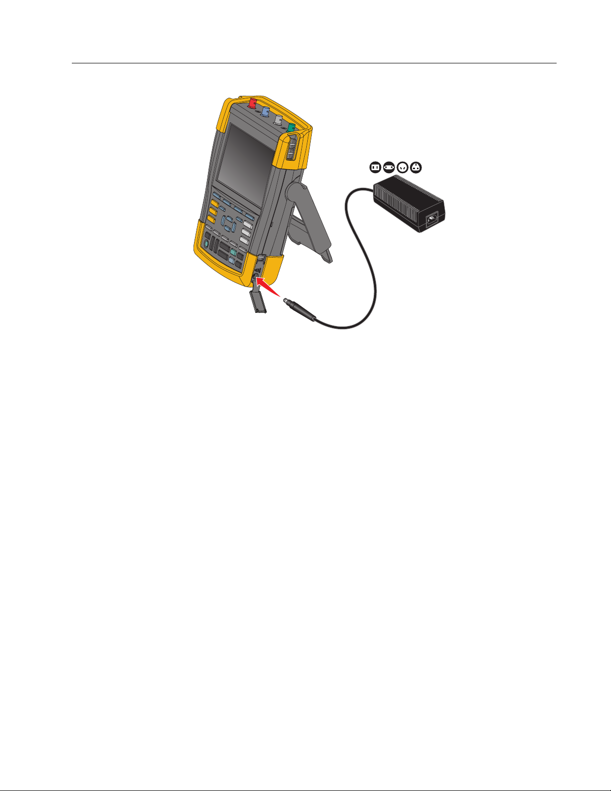
Figure 46. Charging the Batteries

ScopeMeter® Test Tool

Maintenance

Alternatively, you may choose to exchange the battery (Fluke accessory BP290 or BP291) with a
fully charged one, and use the external battery charger EBC290 (optional Fluke accessory).

Battery Pack Replacement

XW Warning

To prevent possible electrical shock, fire, or personal injury, use only the Fluke
BP290 (not recommended for 190-xx4), BP291, or Fluke-recommended equivalent
for replacement.

When no adapter power is supplied, data not yet saved in the test tool memory is maintained if
the battery is replaced within 30 seconds. To avoid loss of data, do one of the following actions
before removing the battery:

• Store the data in the test tool (internal, non-volatile flash memory), on a computer, or a USB

flash drive.

• Connect the power adapter.

85

Find Quality Products Online at: [e-mail]

www.GlobalTestSupply.com

190 Series III

1

A

B

C

D

Users Manual

To install or replace the battery pack:

1. Remove all probes and/or test leads.

2. Remove the standup or fold it to the test tool.

3. Unlock the battery cover. See Figure 47 .

4. Lift the tilt stand. See .

5. Lift the battery cover and remove it. See .

6. For replacement, lift one side of the battery and remove it. See .

7. Install a battery and close the battery cover.

Figure 47. Battery Pack Replacement

86

Find Quality Products Online at: [e-mail]

www.GlobalTestSupply.com

ScopeMeter® Test Tool

 Probe Cal

 Probe Cal Reference

Note

VPS421 does not need adjustment.

Maintenance

Voltage Probe Calibration

To fully meet user specifications, you need to adjust the voltage probes for optimal response. The
calibration consists of a high frequency adjustment and a dc calibration for 10:1 probes and
100:1 probes. The probe calibration matches the probe to the input channel.

To calibrate the 10:1 voltage probes:

1. Press

A to show the input A key labels.

2. Press 3 to open the PROBE ON A menu.

If the correct probe type is already selected (yellow shaded) you can continue at step 5.

3. Use the cursor and E to select Probe Type: Voltage and Attenuation: 10:1.

4. Press 3 to open the PROBE ON A menu again.

5. Press 1 to select PROBE CAL...

Note

It is necessary to connect both the hook clip and the zero reference contact.

A message appears asking you whether to start the 10:1 probe calibration.

6. Press 4 to start the probe calibration.

A message appears telling you how to connect the probe. Connect the red 10:1 voltage probe
to input A and to the probe calibration reference signal. See Figure 48.

Figure 48. Voltage Probe Adjustment

Find Quality Products Online at: [e-mail]

www.GlobalTestSupply.com

87

190 Series III

Users Manual

7. Adjust the trimmer screw in the probe housing until a pure square wave shows on the display.

For instructions to access the trimmer screw in the probe housing, see the instruction sheet
for the probe.

8. Press 4 to continue with DC calibration. Automatic DC calibration is only possible for
10:1 voltage probes.

The test tool automatically calibrates itself to the probe. During calibration you should not
touch the probe. A message indicates when the DC calibration has completed successfully.

9. Press 4 to exit.

Repeat the procedure for the blue 10:1 voltage probe on input B, the gray 10:1 voltage probe on
input C and the green 10:1 voltage probe on input D.

Note

When using 100:1 voltage probes, choose 100:1 attenuation to perform an adjustment.
100:1 voltage probes require DC-calibration. Trimmer adjustment is not available.

Version and Calibration Information

You can display version number and calibration date:

1. Press

2. Press 3 to open the VERSION & CALIBRATION screen.

3. Press 4 to close the screen.

The screen gives you information about the model number with software version, the serial
number, the calibration number with latest calibration date, and installed (software) options. The
LICENSE INFO key opens a screen with information about the Open Source Software license.
The test tool specifications are based on a 1 year calibration cycle. Recalibration must be carried
out by qualified personnel. Contact your local Fluke representative for recalibration.

U to show the USER key labels.

88

Find Quality Products Online at: [e-mail]

www.GlobalTestSupply.com

ScopeMeter® Test Tool

Maintenance

Battery Information

The battery information screen provides information about the battery status and battery serial
number.

To display the battery information:

1. Press

2. Press 3 to open the VERSION & CALIBRATION screen.

3. Press 1 to open the BATTERY INFORMATION menu.

4. Press 4 to return to the previous screen.

Level indicates the available battery capacity as a percentage of the present maximum battery
capacity. Time to Empty indicates a calculated estimate for the operating time that reamins.

U to show the USER key labels.

Replacement Parts

Ta bl e 5 is a list of replacement parts. To order replacement parts, contact your Fluke

representative.

Table 5. Replacement Parts

Description Part Number

Universal Mains-Power Adapter BC190/830

Test Leads with test pins (one red, one black) TL175

Voltage Probe Set (Red or Blue or Gray or Green) The set includes the
following items (not available separately):

• 10:1 Voltage Probe, 500 MHz

• Hook Clip for Probe Tip

• Ground Lead with Mini Alligator Clip

• Ground Spring for Probe Tip

• Insulation Sleeve

VPS410-II-R (red)
VPS410-II-B (blue)
VPS410-II-G (gray)
VPS410-II-V (green)

Voltage Probe Set (Red or Blue or Gray or Green) The set includes the
following items (not available separately):

• 100:1 Voltage Probe with 4 mm Probe Tip, 150 MHz

• Hook Clip for 4 mm Probe Tip (black)

• Reference Lead for 4 mm Probe Tip with 4 mm Banana Plug

• Alligator Clip (x2) for 4 mm Probe Tip

• Test Probe for 4 mm Probe Tip

Find Quality Products Online at: [e-mail]

www.GlobalTestSupply.com

VPS421-R
VPS421-G
VPS421-B
VPS421-V

89

190 Series III

Users Manual

Table 5. Replacement Parts (cont.)

Description Part Number

Replacement Accessories Set for Voltage Probe VPS421 RS421

Replacement Accessories Set for Voltage Probe VPS410 and
VPS410-II

Magnet Probe (x4) MP1

BNC Feedthrough 50 Ω (1 Watt) terminator (set of two pieces, black) TRM50

Li-ion battery (26 Wh, not recommended for models 190-xx4) BP290

Li-ion battery (54 Wh) BP291

Hangstrap 946769

RS400

Optional Accessories

Ta bl e 6 is a list of optional accessories. F

Table 6. Optional Accessories

Description Part Number

Voltage Probe Set, designed for use with the Fluke 190-50x test tool.

Set includes the following items (not available separately):

• 10:1 Voltage Probe, 500 MHz (red or blue or gray or green)

• Hook Clip for Probe Tip (black)

• Ground Lead with Mini Alligator Clip (black)

• Ground Spring for Probe Tip (black)

• Insulation Sleeve (black)

• Probe Tip to BNC Adapter

VPS510-R (red)
VPS510-B (blue)
VPS510-G (gray)
VPS510-V (green)

Replacement Set for Voltage Probe VPS510

Set includes the following items (not available separately):

• 1x Hook Clip for Probe Tip (black)

• 1x Ground Lead with Mini Alligator Clip (black)

• 2x Ground Spring for Probe Tip (black)

• 2x Insulation Sleeve for Probe Tip (black)

• 2x Probe Tip to BNC Adapter

Probe Accessory Extension Set: VPS410, VPS410-II

The set includes the following items (not available separately):

• 1x Industrial Alligator for Probe Tip (black)

• 1x 2-mm Test Probe for Probe Tip (black)

• 1x 4-mm Test Probe for Probe Tip (black)

• 1x Industrial Alligator for 4 mm Banana Jack (black)

• 1x Ground Lead with 4-mm Banana Jack (black)

90

RS500

AS400

Find Quality Products Online at: [e-mail]

www.GlobalTestSupply.com

Table 6. Optional Accessories (cont.)

Description Part Number

Software & Carrying Case Kit.

Set contains the following parts:

• FlukeView 2 Software activation key, to convert the FlukeView 2
demo version into an operational version.

• WiFi Adapter (DWA131)

• Hard Shell Carrying Case CXT293

ScopeMeter® Test Tool

Maintenance

SCC293

FlukeView Software for Windows activation key (converts FlukeView 2
DEMO status into Full Version status)

Hard Shell Carrying Case CXT293

External Battery Charger, charges BP290/BP291 externally using
BC190

Hanging Hook; allows the test tool to be hung on a cabinet door or
separation wall.

50 Ohm Coaxial Cable Set; includes 3 cables (1 red, 1 gray, 1 black),

1.5 m length with safety designed insulated BNC connectors.

50 Ohm Coaxial Cable Set; includes 3 cables (1 red, 1 gray, 1 black),

0.5 m length with safety designed insulated BNC connectors.

Safety designed BNC T-piece, Male BNC to dual female BNC (fully
isolated).

BNC Feedthrough 50 Ohm (1 W) terminator (set of two pieces, black) TRM50

10:1 200 MHz voltage probe, 2.5 m

1:1 30 MHz voltage probe, 1.2 m VPS101

Dual Banana Plug male to female BNC PM9081

FlukeView-2

EBC290

HH290

PM9091

PM9092

PM9093

VPS212-R (red),
VPS212-G (gray)

Dual Banana Jack female to male BNC PM9082

Automotive Troubleshooting Kit SCC298

91

Find Quality Products Online at: [e-mail]

www.GlobalTestSupply.com

190 Series III

Users Manual

Troubleshooting

Test Tool Shuts Down After a Short Time

• The batteries may be empty. Check the battery symbol at the top right of the screen. h
indicates that the batteries are empty and must be charged. Connect the BC190 power
adapter.

• The test tool is still on but the Display Auto Off timer is active. To turn the display on press any
key (restarts the Display AUTO-off timer), or connect the BC190 power adapter.

• The power down timer is active.

• Press ON/OFF to turn on the test tool.

•See Power Down Timer.

Screen Remains Black

• Make sure that the test tool is on (press O and wait several seconds).

• The display Auto Off Timer is active. To turn on the display press any key (restarts the Display
AUTO-off Timer), or connect the BC190 power adapter.

•See Display AUTO-off Timer.

Test Tool Cannot Be Turned Off

If the test tool cannot be turned off due to a software hangup, push the ON/OFF key for at least
5 seconds.

FlukeView 2 Does Not Recognize the Test Tool

• Make sure that the test tool is turned on.

• Make sure that the interface cable is properly connected between the test tool and the PC or
the WiFi connection is set up correctly. Use only the test tool mini USB port for
communication with a computer.

• Make sure that no SAVE/RECALL/COPY/MOVE action from or to a USB-stick is being
performed.

• Make sure that the USB drivers have been correctly installed. USB Drivers.

Battery Operated Fluke Accessories Do Not Function

When using battery operated Fluke accessories, always first check the battery condition of the
accessory with a Fluke multimeter or follow the procedure given for that particular accessory.

92

Find Quality Products Online at: [e-mail]

www.GlobalTestSupply.com