

Page 1
FLIR Camera Adjustments
FLIR Commercial Systems
70 Castilian Drive
Goleta, CA 93117
Phone: +1.805.964.9797
www.flir.com
LWIR Video Camera
Application Note
Document Number: 102-PS242-100-01
Version: 110
Issue Date: June 2014
Page 2

FLIR Camera Adjustments
Table of Contents
FLIR Camera Adjustments ........................................................................................................................... 1
LWIR Video Camera .................................................................................................................................... 1
Application Note ........................................................................................................................................... 1
Document Number: 102-PS242-100-01 ....................................................................................................... 1
1.0 Document .......................................................................................................................................... 4
1.1 Revision History ........................................................................................................................... 4
1.2 Scope ............................................................................................................................................. 4
2.0 Automatic AGC Parameters.............................................................................................................. 5
2.1 Introduction to Histograms ........................................................................................................... 6
2.2 Linear Histogram .......................................................................................................................... 7
2.3 Plateau Histogram Equalization .................................................................................................... 8
2.4 Information-based and Information-based equalization ............................................................. 20
2.5 Legacy AGC modes .................................................................................................................... 21
2.5 Digital Data Enhancement (DDE) .............................................................................................. 22
3.0 LUT Palettes and Polarity ............................................................................................................... 24
4.0 FFC Warning Indicator ................................................................................................................... 27
Table of Figures
Figure 1: 14-bit Histogram ............................................................................................................................ 6
Figure 2: Image of scene ............................................................................................................................... 7
Figure 3: Linear AGC, ITT Mean: 127, Max Gain: 8 ................................................................................... 7
Figure 4: Illustration of the Linear-Histogram Mapping Function ............................................................. 8
Figure 5: Plateau: 150, ITT Mean: 127, Max Gain: 8 ................................................................................... 9
Figure 6: Image Transform Table for Linear and Plateau algorithms......................................................... 10
Figure 7: Plateau: 250, ITT: 110, Max Gain: 8 ........................................................................................... 11
Figure 8: Plateau: 250, ITT: 150, Max Gain: 8 ........................................................................................... 11
Figure 9: Low contrast scene in 14-bit space. ............................................................................................. 12
Figure 10: Plateau: 250, ITT: 127, Max Gain: 8 ......................................................................................... 12
Figure 11: Low contrast Scene: default settings ......................................................................................... 12
Figure 12: Plateau: 250, ITT: 127, Max Gain: 25 ....................................................................................... 13
Figure 13: Low contrast scene: high gain ................................................................................................... 13
Figure 14: Plateau: 250, ITT: 127, Max Gain: 50 ....................................................................................... 13
Figure 15: Low Contrast Scene: very high gain ......................................................................................... 13
Figure 16: Illustration of Plateau Value .................................................................................................... 14
Figure 17: Illustration of Maximum Gain in a Bland Image .................................................................... 15
Figure 18: Illustration of ITT Midpoint .................................................................................................... 16
Page 3

FLIR Camera Adjustments
102-PS242-100-01 Rev110
June 2014
Page 3 of 28
Figure 19: Illustration of Active Contrast Enhancement (ACE) ................................................................. 17
Figure 20: Illustration of Smart Scene Optimization (SSO) ....................................................................... 18
Figure 21: Illustration of ROI ................................................................................................................... 19
Figure 22: Illustration of the difference between Plateau Equalization, Information-based, and
Information-based Equalization algorithms ................................................................................................ 21
Figure 23: Illustration of Information Threshold ........................................................................................ 21
Figure 24: Illustration of Noise Suppression with DDE ........................................................................... 23
Figure 25: Illustration of Detail Enhancement with DDE ........................................................................ 23
Figure 26: White Hot .................................................................................................................................. 24
Figure 27: Black Hot ................................................................................................................................... 24
Figure 28: Look-Up Table Options (Without Isotherms) ........................................................................... 25
Figure 20: Isotherm LUT Scale Example ................................................................................................... 26
Figure 21: Look-Up Table Options (with Isotherms) ................................................................................. 27
Figure 29: FFC Warning ............................................................................................................................. 28
Page 4
FLIR Camera Adjustments
102-PS242-100-01 Rev110
June 2014
Page 4 of 28
Version
Date
Comments
100
10/25/2011
Initial Release
110
6/20/2014
Updates for the Tau 2.7 and Quark 2 release
Document Title
Document
Number
Description
Tau Quick Start Guide
102-PS242-01
Quick Start Guide for first-time use
Quark Quick Start Guide
102-PS241-01
Quick Start Guide for first-time use
FLIR Camera Controller GUI
User’s Guide
102-PS242-02
Detailed Descriptions for functions and adjustments
for FLIR cameras using the FLIR Camera Controller
GUI
Tau 2 Product Specification
102-PS242-40
Product specification and feature description
Quark Product Specification
102-PS241-40
Product specification and feature description
Tau 2 Electrical IDD
102-PS242-41
Written for Electrical Engineers to have all necessary
information to interface to a Tau 2 camera
Quark Electrical IDD
102-PS241-41
Written for Electrical Engineers to have all necessary
information to interface to a Tau 2 camera
Tau 2/Quark Software IDD
102-PS242-43
Written for Software Engineers to have all necessary
information for serial control of Tau 2 and Quark
Assorted Mechanical
Drawings and Models
Various
There are drawings and 3D models for various
camera configurations for mechanical integration
Application Notes
Various
Written for Systems Engineers and general users of
advanced features such as Gain Calibration,
Supplemental FFC Calibration, NVFFC Calibration,
Camera Link, On-Screen Symbology, AGC/DDE
explanation, Camera Mounting, Spectral Response,
Optical Interface for lens design, and others.
1.0 Document
1.1 Revision History
1.2 Scope
This note is intended to provide a better understanding of FLIR image processing algorithms. Once these
are well understood by the user, the camera can be optimized to give the best possible image for a given
scenario. This document applies to the FLIR Quark, Quark 2, Tau, Tau 2 and Neutrino cameras. These
cores can be found in most FLIR Commercial Systems products.
The FLIR website will have the newest version of this document as well as offer access to many other
supplemental resources: http://www.flir.com/cvs/cores/resources/
Here is a sample of some of the resources that can be found:
There is also a large amount of information in the Frequently Asked Questions (FAQ) section on the
FLIR website: http://www.flir.com/cvs/cores/knowledgebase/. Additionally, a FLIR Applications
Engineer can be contacted at 888.747.FLIR (888.747.3547).
Page 5

FLIR Camera Adjustments
102-PS242-100-01 Rev110
June 2014
Page 5 of 28
2.0 Automatic AGC Parameters
The first thing to understand is that the detector data is directly streamed from the sensor as 14-bit values
for each pixel in the array. The analog image is displayed using 8-bit values and almost all commercial
displays are 8-bit devices. In other words the video is displayed on a 0-255 scale rather than the full 016384 resolution of the sensor. This means that there must be some compression to get the data into a
format that can be displayed. Throughout this note, there are histograms that are represented in Signal vs.
Number of Pixels. A histogram is a sorting of pixel values into intensity “bins”. What this means is the
bit value (which increases as pixels get brighter) is on the x-axis and the number of pixels in the image
that have that bit value is on the y-axis. This is a way of plotting image data in order to illustrate which
are the most significant intensity values. The algorithms attempt to compress the data in a meaningful
way that preserves as much of the image content as possible.
The Tau 2 core provides multiple AGC algorithms used to transform 14-bit data to 8-bit. These options
include the following, with associated parameters shown below each algorithm:
Plateau equalization
o Plateau value
o Maximum gain
o ITT midpoint
o ACE threshold
o SSO value
o Tail rejection
o Region of Interest (ROI)
o IIR filter
Information-based and Information-based equalization
o Information-based Threshold
Linear histogram
o ITT midpoint
o ROI
o IIR filter
Manual
o Brightness
o Contrast
o IIR filter
Page 6
FLIR Camera Adjustments
102-PS242-100-01 Rev110
June 2014
Page 6 of 28
1 2 3
Auto-bright
o Brightness
o Contrast
o IIR filter
Once-bright
o Brightness bias
o Contrast
o IIR filter
Note: FLIR highly recommends that each customer optimize AGC settings for each particular
application. “Preferred” AGC settings are highly subjective and vary considerably depending upon
scene content and user preferences. Generally speaking, FLIR recommends the plateau equalization
algorithm, but there are scenarios where each of the other algorithms may be better suited. The FLIR
GUI provides auto presets that can be used to tune AGC to the specific scene.
2.1 Introduction to Histograms
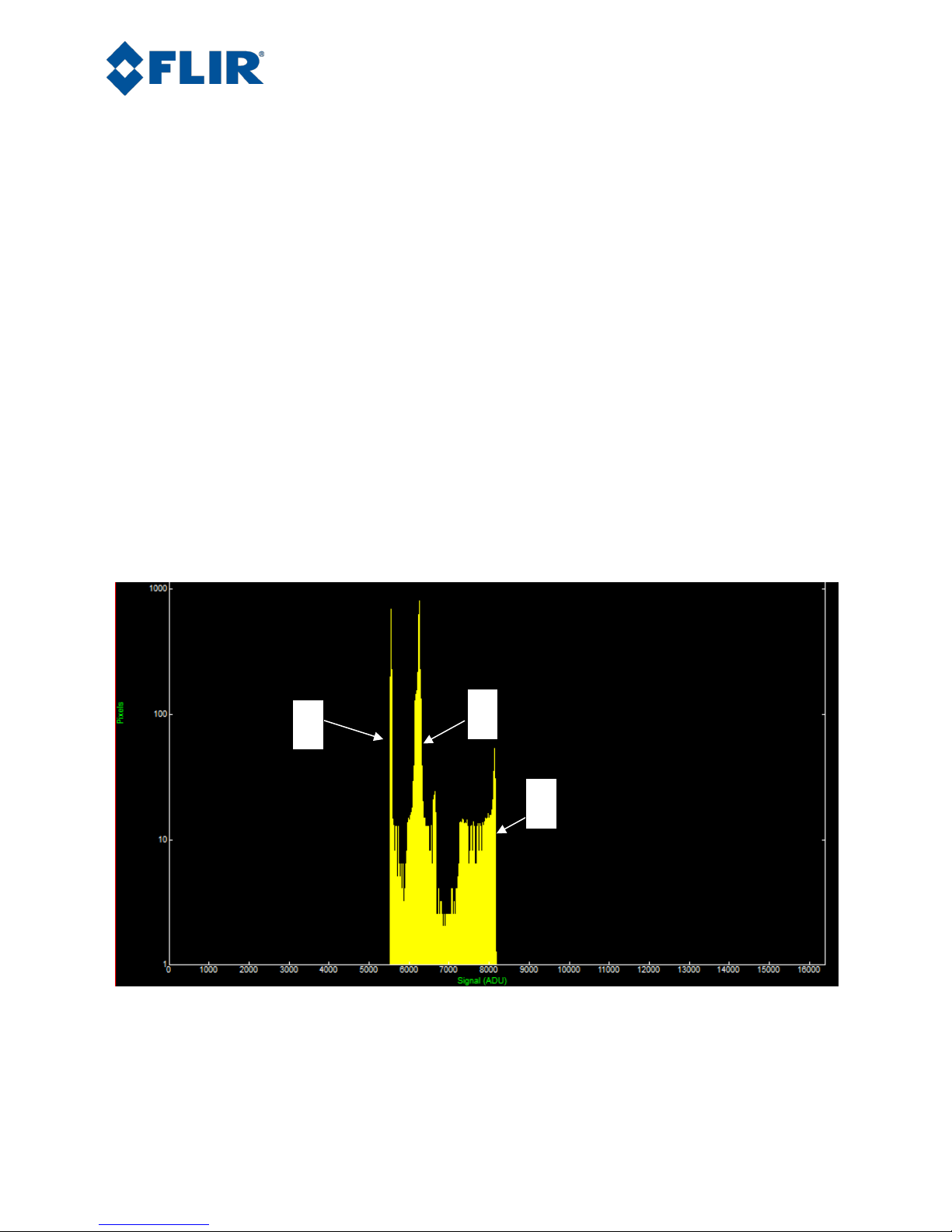
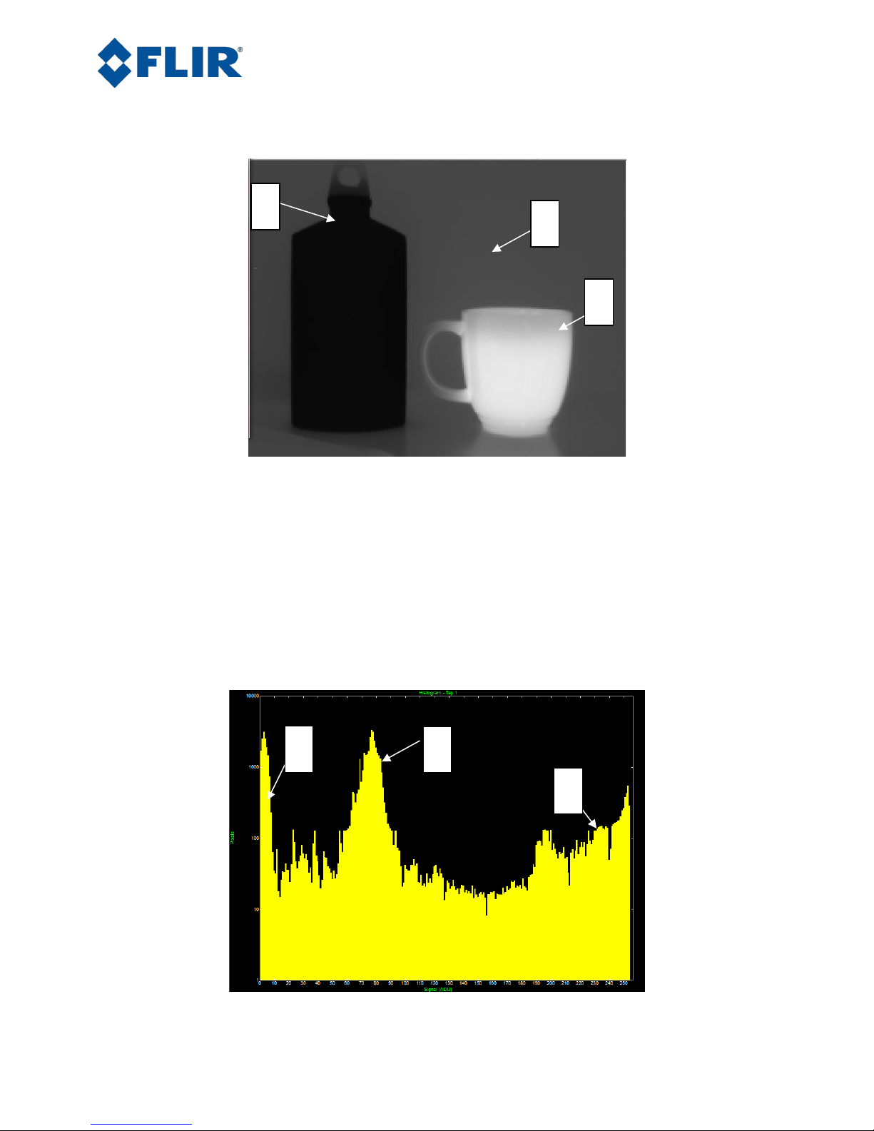
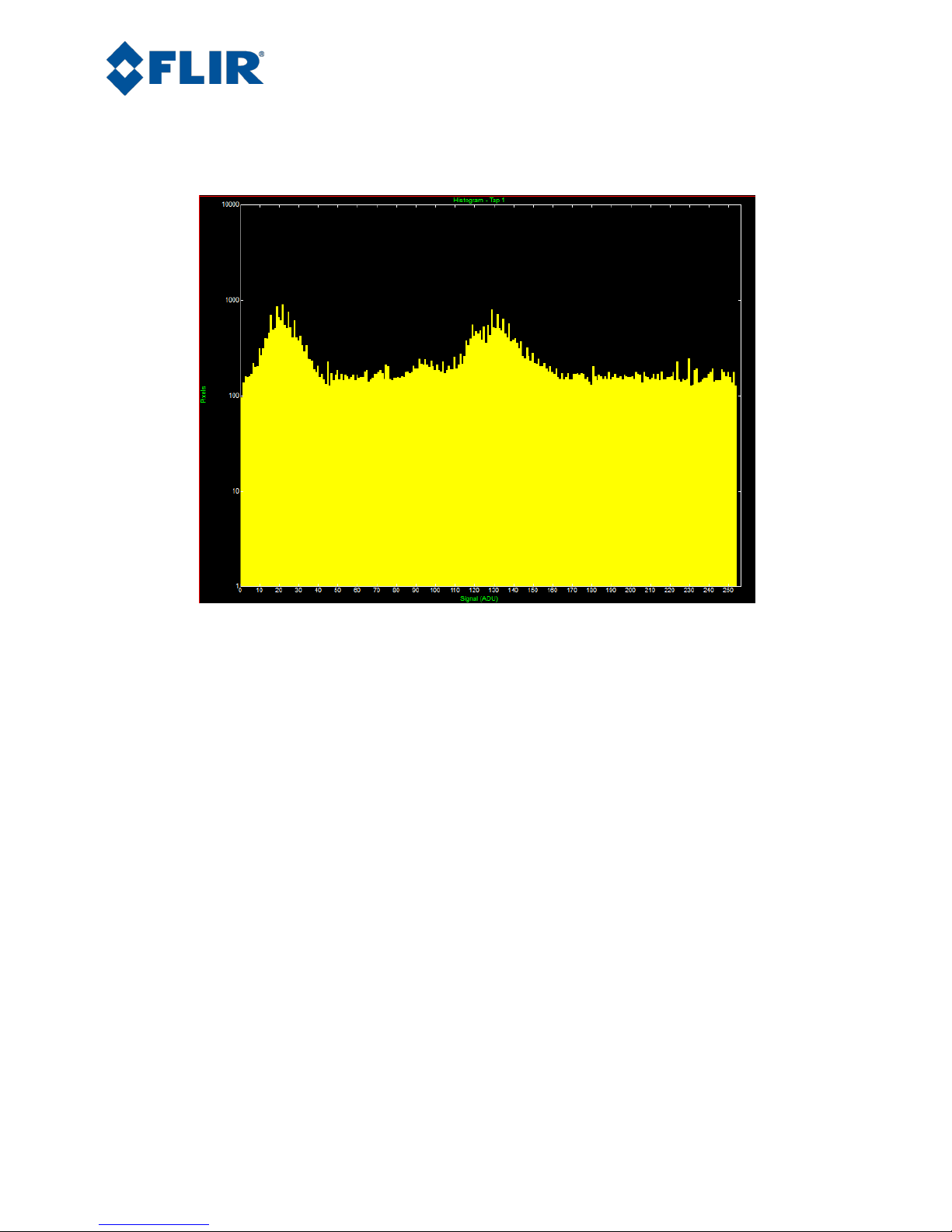
The following histogram is the 14-bit data taken from a Tau 320 with a cold water bottle, a midtemperature wall, and a hot coffee mug in the scene. These three objects can be seen in the data histogram
as three separate peaks. The lowest bit values, which are farthest to the left in the histogram, are the
coldest pixels in the scene. The values in 14-bit space range from 0 to 16384.
The following image is associated with this histogram. You can see the cold, black water bottle, the grey
background, and the hot, white coffee mug. You can also see that the water bottle is fairly uniform and
Figure 1: 14-bit Histogram
Page 7
FLIR Camera Adjustments
102-PS242-100-01 Rev110
June 2014
Page 7 of 28
1
2
3
1 2 3
has a narrow spike whereas the mug has different temperatures in the handle and above the coffee line.
For this reason, the data is more spread in the histogram at point 3.
Figure 2: Image of scene
2.2 Linear Histogram
The first and simplest method to translate the data into 8-bit space is using a linear algorithm. Although
this algorithm is not typically used, it will help illustrate the concept of using a transfer funciton to map
from one space to another. A typical linear intensity transfer table will map the middle 90% of the
histogram to 8 bit space. The bottom and top 5% are discarded. This algorithm finds the interesting
portion of the data and crops above and below it. The following histogram is a representation of the same
scene in 8-bit space. Notice the three peaks from the 14-bit data represented in 8-bit space and that the
values on the x-axis now range from 0-255 rather than 0-16384.
Figure 3: Linear AGC, ITT Mean: 127, Max Gain: 8
Page 8
FLIR Camera Adjustments
102-PS242-100-01 Rev110
June 2014
Page 8 of 28
(a) ITT Midpoint = 128
(b) ITT Midpoint = 96
14bit_5%
14bit_95%
Avg(14bit_5%, 14bit_95%)
specified
ITT Midpoint
14bit_5%
14bit_95%
Avg(14bit_5%, 14bit_95%)
specified
ITT Midpoint
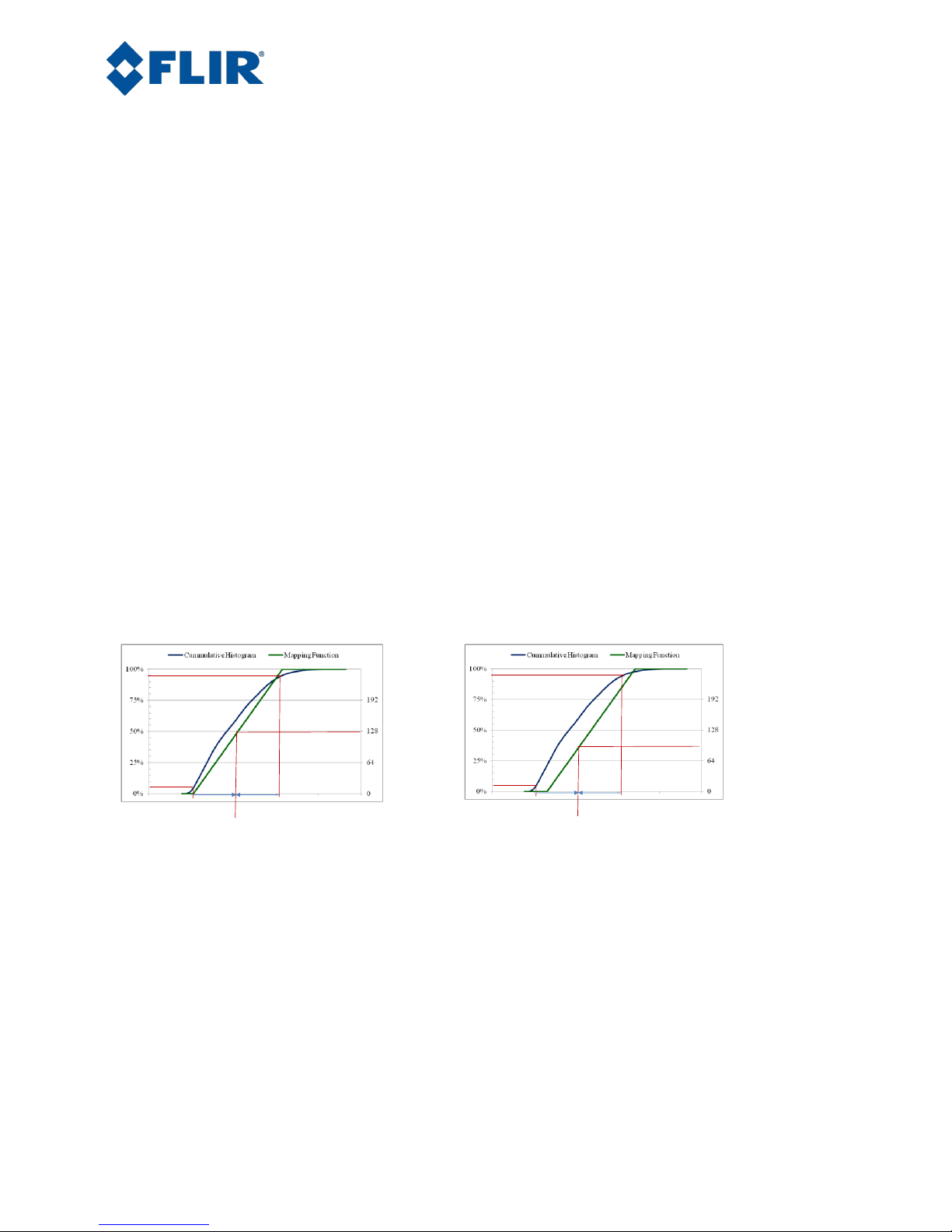
The linear histogram algorithm performs a linear transformation from 14-bit to 8-bit of the form:
8biti = m * 14biti + b
The slope of the transformation is computed automatically based on the ROI histogram:
m = 255 / (14bit_(100 – Tail Rejection)% - 14bit_(Tail Rejection)%),
where 14bit_(Tail Rejection)% is the 14-bit value corresponding to the user selectable tail rejection
percentage point on the cumulative ROI histogram and 14bit_(100 – Tail Rejection)% is the value
corresponding to the difference between 100% and the user selectable tail rejection percentage point in
Tau 2.7 and Quark 2.0.
The offset is then computed as
b = ITT midpoint - avg(14bit_(100 – Tail Rejection)%, 14bit_(Tail Rejection)%),* m
In other words, the algorithm attempts to map the midway point between the top and bottom tail rejection
points on the cumulative histogram to the specified ITT midpoint, as shown in Figure 4 for the case in
which the tail rejection parameter selected is 5%. The 8-bit values resulting from the above equations are
clipped to a minimum value of 0 and a maximum value of 255.
Figure 4: Illustration of the Linear-Histogram Mapping Function
2.3 Plateau Histogram Equalization
The Plateau Histogram Equalization algorithm seeks to maximize the dynamic range available for the
content of the scene. It does this using a transfer function that is based on the number of pixels that are in
each bin and allocating more 8-bit range for that bin. The Plateau value is the pixels/bin limit when the
transfer function is maximized. When this number is small, the Automatic AGC will approach a linear
algorithm that preserves a linear mapping between the 14-bit and 8-bit data. The goal of the Automatic
algorithm is to try and make each of the 255 bins have the same number of pixels in it, which should give
the best contrast for the given scene. When the plateau value is higher, the algorithm is more able to
Page 9
FLIR Camera Adjustments
102-PS242-100-01 Rev110
June 2014
Page 9 of 28
redistribute the data to achieve this goal. This prevents wasted levels of grey on regions that have no
scene content and can visually be seen in the histograms by noticing that peaks are much smoother and
the data is spread much more evenly.
Figure 5: Plateau: 150, ITT Mean: 127, Max Gain: 8
Compare to Linear Histogram in Figure 3
The following plot shows the Image Transform Table for both Linear and Plateau Histogram
Equalization. The 14-bit value on the x-axis will map to the 8-bit value on the y-axis where the
conversion is plotted. In 14-bit regions with low contrast, the curve is much flatter and there are not as
many 8-bit values consumed. In high detail regions, the curve is steep and more 8-bit values are used.
Page 10

FLIR Camera Adjustments
102-PS242-100-01 Rev110
June 2014
Page 10 of 28
Linear 14 to 8 bit
Histogram Equalized
Lots of Contrast
Low Contrast
Low Contrast
Figure 6: Image Transform Table for Linear and Plateau algorithms
In many applications, there are objects with different temperatures that all need to have contrast. In this
case, the plateau value can be increased from the default setting of 150 to 250 or 300, depending on the
content of the scene. This will provide the algorithm with more flexibility to generate an image with high
contrast for both foreground and background targets. In applications where there is a large object of a
small temperature range and the background is not important, lowering the plateau value to 100 or 50 will
dedicate more contrast to the foreground object and the background will have less. This can also be done
when an AGC ROI is used to discard scene content that is not important.
It is important to note that higher plateau value distorts the correlation between physical temperature of
the scene and level of grey in the image, which is preserved in a linear histogram.
The ITT Mean sets the midpoint of the Image Transform Table and is applied after the histogram
equalization on the 8-bit data. This can be thought of as an offset that shifts the entire distribution to the
left or the right and directly affects the brightness of the image. It is important to notice that when the data
is shifted, it is cropped and it is not stretched to fill the 8-bit range. This means that you are losing data by
shifting, but the data on the top and bottom may not be the most important. Increasing the Plateau Value,
as seen above, typically raises the perceived brightness of the scene. This could be counteracted by
lowering the ITT Mean from the default of 127 to 120.
Page 11

FLIR Camera Adjustments
102-PS242-100-01 Rev110
June 2014
Page 11 of 28
Figure 7: Plateau: 250, ITT: 110, Max Gain: 8
Figure 8: Plateau: 250, ITT: 150, Max Gain: 8
It is also important to note that changes in levels of grey are more perceptible to a human observer at
lower levels of illumination. This is because a change from 5 to 10 counts is 100% and a change from 245
to 250 is about 2%. By lowering the ITT Mean, you can shift the luminance to a lower value so that a
human observer will be more capable of seeing small changes in the scene. If you are using analytics, the
performance will not likely be improved by this change and the default setting of 127 is recommended.
The final AGC parameter is the Max Gain. To demonstrate this, it will be better to look at a scene with
very low contrast. The scene used was a uniform wall with an empty paper cup that was slightly warmer
than the wall. Notice the very narrow spike in the 14-bit data and the very small bump just to the right of
the spike.
Page 12

FLIR Camera Adjustments
102-PS242-100-01 Rev110
June 2014
Page 12 of 28
Figure 10: Plateau: 250, ITT: 127, Max Gain: 8
Figure 11: Low contrast Scene: default settings
His
Figure 9: Low contrast scene in 14-bit space.
The large spike from the wall is the same value as in initial histogram.
The following histogram shows the 8-bit data with the default Max Gain setting of 8. Notice that
there is a large amount of unused levels of grey on the left and right of the signal. The maximum gain
setting sets the upper limit of gain that the algorithm can use as it attempts to stretch the data to fill the
full 8-bit range. If the scene has a high level of contrast, it will use much less gain than the maximum gain
setting. In typical applications, this value can be increased from the default of 8 to 12 or 15. Analytics that
are not affected by spatial noise might tolerate higher values around 25 or 30. Values below are used for
demonstration and do not represent typical settings.
Page 13

FLIR Camera Adjustments
102-PS242-100-01 Rev110
June 2014
Page 13 of 28
Figure 12: Plateau: 250, ITT: 127, Max Gain: 25
Figure 13: Low contrast scene: high gain
Figure 14: Plateau: 250, ITT: 127, Max Gain: 50
Figure 15: Low Contrast Scene: very high gain
Lo
The plateau equalization algorithm performs a non-linear transformation from 14-bit to 8-bit based on
image histogram. It is a variant of classic histogram equalization, an algorithm that maps 14-bit to 8-bit
using the cumulative histogram of the 14-bit image as the mapping function. In classic histogram
equalization, an image comprised of 60% sky will devote 60% of the available 8-bit shades to the sky,
leaving only 40% for the remainder of the image. Plateau equalization limits the maximum number of
gray shades devoted to any particular portion of the scene by clipping the histogram (via the plateau
value) and limiting the maximum slope of the mapping function (via the maximum gain value). It also
provides an ITT midpoint value that allows mean brightness of the 8-bit image to be specified. The Tau
2.7 release includes the ability to allot a linear portion to the histogram (via Smart Scene Optimization),
include an irradiance dependent contrast adjustment (via Active Contrast Enhancement), and specify
outlier rejection (via Tail Rejection). The description below provides explanations of each of these
parameters.
Page 14

FLIR Camera Adjustments
102-PS242-100-01 Rev110
June 2014
Page 14 of 28
(a) Plateau Value = 1000
(b) Plateau Value = 10
(c) 8bit Histogram for Plateau Value = 1000
(d) 8-bit Histogram for Plateau Value = 10
Plateau value. When plateau value is set high, the algorithm approaches the behavior of classic histogram
equalization – gray shades are distributed proportionally to the cumulative histogram, and more gray
shades will be devoted to large areas of similar temperature in a given scene. On the other hand, when
plateau value is set low, the algorithm behaves more like a linear AGC algorithm – there is little
“compression” in the resulting 8-bit histogram. The figures below illustrate both of the cases.
(Notice details in the sidewalk in the left image whereas more gray shades are available for the
Figure 16: Illustration of Plateau Value
pedestrians in the right image.)
Page 15

FLIR Camera Adjustments
102-PS242-100-01 Rev110
June 2014
Page 15 of 28
(a) Maximum Gain = 6
(b) Maximum Gain = 24
(c) 8bit Histogram for Max. Gain = 6
(d) 8bit Histogram for Max. Gain = 24
Maximum Gain. For scenes with high dynamic range (that is, wide 14-bit histogram), the maximum gain
parameter has little effect. For a very bland scene, on the other hand, it can significantly affect the
contrast of the resulting image. Figure 17 provides an example.
Figure 17: Illustration of Maximum Gain in a Bland Image
(Notice more details but also greater fixed-pattern noise in the right image.)
Page 16

FLIR Camera Adjustments
102-PS242-100-01 Rev110
June 2014
Page 16 of 28
(a) ITT Midpoint = 127
(b) ITT Midpoint = 96
(c) 8bit Histogram for ITT Midpoint = 127
(d) 8bit Histogram for ITT Midpoint = 96
ITT Midpoint. The ITT Midpoint can be used to shift the 8-bit histogram darker or brighter. The
nominal value is 128. A lower value causes a darker image, as shown in Figure 18. A darker image can
help improve the perceived contrast, but it is important to note that more of the displayed image may be
railed (8bit value = 0 or 255) by moving the midpoint away from 128. This can be seen in the histogram
of Figure 18.
(Notice image on the right is darker. Notice in the histogram on the right that far more pixels have
a value of 0 and that no pixels have a value between 224 and 255.)
Figure 18: Illustration of ITT Midpoint
Page 17

FLIR Camera Adjustments
102-PS242-100-01 Rev110
June 2014
Page 17 of 28
ACE Threshold. The Active Contrast Enhancement (ACE) feature provides a contrast adjustment
dependent on the relative scene temperature. ACE thresholds greater than 0 impart more contrast to hotter
scene content and decrease contrast for colder scene content (e.g. sky or ocean). ACE threshold less than
0 do the opposite by decreasing contrast for hotter scene content and leaving more of the gray-scale
shades to represent the colder scene content. Figure 19 illustrates the effects of ACE. FLIR recommends a
conservative setting of 3 for generic use-case scenarios.
(a) ACE threshold = -4 (b) ACE threshold = 0 (neutral) (c) ACE threshold = 8
Figure 19: Illustration of Active Contrast Enhancement (ACE)
SSO Value. The Smart Scene Optimization (SSO) value defines the percentage of the histogram that will
be allotted a linear mapping. Enabling this feature facilitates the avoidance of irradiance level
compression, which is specifically important for bi-modal scenes. With SSO enabled, the radiometric
aspects of an image are better preserved (i.e. the difference in gray shades between two objects is more
representative of the difference in temperature). While radiometry is better preserved with this feature, the
compromise is the optimization in local contrast. Figure 20 illustrates the effects of SSO. In the left
image, SSO is disabled and the hot object and person get mapped to two shades of gray next to one
another causing a “washed out” effect and making it appear as though the person and fire are similar in
temperature. In the right image, SSO is enabled, and the hot object and person are decompressed with
gray shades separating them.
Page 18

FLIR Camera Adjustments
102-PS242-100-01 Rev110
June 2014
Page 18 of 28
(a) SSO = 0% (disabled) (b) SSO = 30%
(c) 8bit Histogram of SSO = 0% (disabled) (d) 8bit Histogram of SSO = 30%
Figure 20: Illustration of Smart Scene Optimization (SSO)
Tail Rejection. The tail rejection parameter defines the percentage of the total number of pixels in the
array that will be excluded prior to histogram equalization. The user-selected percentage of pixels will be
removed from both the bottom and top of the 14-bit histogram prior to AGC. This feature is useful for
excluding outliers and the most extreme portions of the scene that may be of less interest. FLIR
recommends tail rejection settings less than 1% to avoid the exclusion of important scene content.
Region of Interest (ROI). In some situations, it is desirable to have the AGC algorithm ignore a portion
of the scene when collecting the histogram. For example, if the Tau 2 core is rigidly mounted such that
the sky will always appear in the upper portion of the image, it may be desirable to leave that portion of
the scene out of the histogram so that the AGC can better optimize the display of the remainder of the
image. This is illustrated in Figure 21. Similarly for a hand-held application, it may be desirable to
optimize the display of the central portion of the image. For those applications, it is possible to specify a
region of interest (ROI) beyond which data is ignored when collecting the image histogram. Any scene
content located outside of the ROI will therefore not affect the AGC algorithm. (Note: this does not mean
the portion outside of the ROI is not displayed, just that the portion outside does not factor into the
optimization of the image.)
Page 19

FLIR Camera Adjustments
102-PS242-100-01 Rev110
June 2014
Page 19 of 28
(b) ROI = Full Image
(b) Sky excluded from ROI
For Tau 2.0, separate ROI are automatically applied for un-zoom, 2X, 4X, and 8X zoom. Coordinates for
the ROI are as follows:
Top / Bottom: 0 = center of the display, negative values are above center, positive values are below center,
units are in pixels
Left / Right: 0 = center of display, negative values are left of center, positive values are right of center,
units are in pixels
For Tau 2.1 and later, a single ROI is specified regardless of zoom (see product specification).
Coordinates for the ROI are as follows:
Top / Bottom: 0 = center of the window, negative values are above center, positive values are below
center, units are percentage of zoom window size (-512 = -50%, +512 = + 50%).
Left / Right: 0 = center of display, negative values are left of center, positive values are right of center,
units are percentage of zoom window size (-512 = -50%, +512 = + 50%).
(Notice the image on the right has more contrast in the portion of the image below the sky.)
Figure 21: Illustration of ROI
Page 20

FLIR Camera Adjustments
102-PS242-100-01 Rev110
June 2014
Page 20 of 28
AGC Filter. The AGC filter is an IIR filter used to adjust how quickly the AGC algorithm reacts to a
change in scene or parameter value. The filter is of the form
n' = n * + n'-1 * (256-)/256
where:
n' = actual filtered output value for the current frame
n = unfiltered output value for the current frame
n'-1 = actual filtered output value for the previous frame
= filter coefficient, user-selectable from 0 to 255
If the AGC filter value is set to a low value, then if a hot object enters the field of view, the AGC will
adjust more slowly to the hot object, resulting in a more gradual transition. In some applications, this can
be more pleasing than a sudden change to background brightness. For the Tau 2.7 release, a filter
coefficient of 255 is a special case for immediate updates, a value of 1 provides the most filtering or
slowest refresh rate, and a value of 0 indicates no further updates to AGC. For previous releases of Tau 2,
a filter coefficient of 0 was a special case for immediate updates, a value of 1 was the most filtering or
slowest refresh rate, and the case for no AGC updates was unavailable.
2.4 Information-based and Information-based equalization
The Tau 2.7 release and subsequent releases include the Information-based algorithms which reserve
more shades of gray for areas with more information or scene content by assigning areas with less
information or scene content lesser gray shades. By assigning lesser gray shades to areas with less
information (e.g. sky, sea, roads) the fixed pattern noise is reduced in these areas also allowing for more
detail to be given to the more interesting portions of the image. Both Information-based algorithms
undergo the plateau equalization process described in the previous section, and therefore all parameters
described also apply.
The differences between the Information-based and Information-based Equalization algorithms are
noteworthy as both have advantages. The Information-based algorithm completely excludes pixels from
histogram equalization if they are below the information threshold (described later in this section). This is
advantageous in that noise is completely removed from areas of the image determined by the algorithm to
not contain information, but scenarios in which the user is attempting to detect small temperature or
emissivity variations are not ideal for this mode because desired information may be lost depending on
the threshold. The Information-based Equalization algorithm includes every pixel independent of scene
information in the histogram equalization process, but simply weights each pixel based on the information
threshold. This mode shows more moderate improvements in scenes with large areas void of information,
but the advantage over the Information-based mode is that scene content will never be removed. Figure
22 shows the Plateau Equalization algorithm on the left for reference and the Information-based and
Information-based Equalization algorithms center and right respectively with information threshold set to
40.
Page 21

FLIR Camera Adjustments
102-PS242-100-01 Rev110
June 2014
Page 21 of 28
(a) Plateau Equalization (b) Information-based (c) Information-based
Equalization
Figure 22: Illustration of the difference between Plateau Equalization, Information-based, and
Information-based Equalization algorithms
Information Threshold. The information threshold parameter defines the difference between neighboring
pixels used to determine whether the local area contains “information” or not. Lower thresholds result in
the algorithm determining that more of the scene contains information, resulting in more areas included in
the Information-based algorithm and given a higher weighting in the Information-based Equalization
algorithm. Decreasing the threshold will result in imagery approaching the appearance of the Plateau
Equalization algorithm. Increasing the threshold will result in a more information-dependent image, that
is the flat portions of the scene (e.g. sky or sea) are given less contrast and the pixels exceeding the
information threshold will be given more contrast.
(a) Information Threshold = 20 (b) Information Threshold = 80
Figure 23: Illustration of Information Threshold
2.5 Legacy AGC modes
Page 22

FLIR Camera Adjustments
102-PS242-100-01 Rev110
June 2014
Page 22 of 28
Manual
The “manual” algorithm performs a linear transformation from 14-bit to 8-bit, with slope based solely on
a specified contrast value and offset based solely on a specified brightness value as shown below:
m = specified contrast / 64
b = 127 – (brightness)*m.
Auto Bright
The auto-bright algorithm is identical to the “manual” algorithm except that brightness value is
automatically and dynamically updated to equal array mean. In other words, the array mean is
automatically mapped to an 8-bit value of 127.
Once Bright
The “once bright” algorithm is identical to the “auto-bright” algorithm except that the offset of the linear
transformation, b, is computed only at the time the algorithm is selected and is not dynamically updated.
It is computed as
b = 127 – (frame mean – brightness bias)*m,
where brightness bias is a user-specified parameter.
2.5 Digital Data Enhancement (DDE)
The Tau 2 core provides an optional “digital-data-enhancement” (DDE) algorithm which can be used to
enhance image details and/or suppress fixed pattern noise. Two modes are available, “manual” and
“dynamic”. The descriptions of each mode are as follows:
Dynamic mode: DDE parameters are computed automatically based on scene contents. DDE
index (which supplants the spatial-threshold parameter used in the manual algorithm) is the only
controlling parameter and ranges from -20 to 100 for Tau 2.7 and later releases, with higher
values representing higher degrees of detail enhancement. If no enhancement is desired, the
value should be set to 0. Values less than 0 soften the image and filter fixed pattern noise, as
exemplified in the figures below. Values greater than 0 sharpen the details in the image. For
previous Tau 1 and Tau 2 releases, the DDE index ranged from 0 to 63, where 0 to 16 softened
the image, 17 was neutral, and 18 to 63 sharpened detail.
Page 23

FLIR Camera Adjustments
102-PS242-100-01 Rev110
June 2014
Page 23 of 28
(a) DDE index = 0
(b) DDE index = -10
(a) DDE index = 0
(b) DDE index = 70
Figure 24: Illustration of Noise Suppression with DDE
(Notice fixed pattern noise is reduced in the image on the right.)
Figure 25: Illustration of Detail Enhancement with DDE
Note: The recommended DDE mode is “dynamic”. “Manual” is provided for customers of
previous FLIR cores that have familiarly with the manual DDE mode.
Page 24

FLIR Camera Adjustments
102-PS242-100-01 Rev110
June 2014
Page 24 of 28
Figure 26: White Hot
Figure 27: Black Hot
Manual mode: The following three parameters are user-specified:
o DDE Gain: ranges from 0 to 65535 for Tau 2.7 and later releases and represents the
magnitude of high-frequency boost
For gain = 0, DDE is disabled
For gain > 0, details are enhanced by gain/2048. In other words, a value of 1
represents a 1/2048 attenuation of details whereas a value of 8192 represents a
4X enhancement of details. Note that gain is also applied globally and locally to
the low frequency portion of the image, and therefore the DDE gain is relative
(therefore users are strongly discouraged from using manual DDE mode).
o DDE threshold: ranges from 0 to 255 and represents the maximum detail magnitude that
is boosted. Details with variance exceeding the threshold are not enhanced. Details with
variance less than the thresholds are enhanced. Values greater than 255 will place the
camera in Dynamic DDE mode with a DDE index of x-255. In this case, DDE Gain and
DDE spatial threshold are adjusted dynamically.
o DDE spatial threshold: ranges from 0 to 15, and represents the threshold of the pre-filter
(smoothing filter) applied to the signal prior to high-frequency boost. The pre-filter
prevents low-magnitude fixed-pattern noise from being amplified. Note that the DDE
spatial threshold also represents the DDE index when in automatic DDE mode.
3.0 LUT Palettes and Polarity
Another topic to discuss is the image LUT (Lookup Table). There are a number of lookup tables that
make the image colored. This is called false color, or pseudocolor. The color is not actually related to
wavelengths of light, but rather the grayscale intensity. The most useful might be the option for White
Hot and Black Hot, which is also called the polarity of the image. The Black Hot palette is a pure
inversion of the 8-bit data where zero becomes the hottest and 255 becomes the coldest. There are some
applications where a Black Hot image allows for more perceived contrast in the image. This is primarily
due to concept discussed earlier about low luminance changes.
Page 25

FLIR Camera Adjustments
102-PS242-100-01 Rev110
June 2014
Page 25 of 28
Cold
Cold
Cold
Cold
Hot
Hot
Hot
Hot
White Hot
Black Hot
Fusion
Rainbow
Cold
Cold
Cold
Cold
Hot
Hot
Hot
Hot
Glowbow
Ironbow1
Ironbow2
Sepia
Cold
Cold
Cold
Cold
Hot
Hot
Hot
Hot
Color1
Color2
Ice Fire
Rain
The Tau2 and Quark cameras contained the normal imaging LUTs which contain 256 colors or greyscale
and map that to the 8-bit AGC data from the cameras. The imaging palettes are shown below. The
palettes only affect the analog and BT.656 outputs of the Quark 1, Tau 2.3 and earlier releases. The
Quark 2 and Tau 2.4 releases and later have an option for color in the CMOS and LVDS 8-bit data.
Figure 28: Look-Up Table Options (Without Isotherms)
The Tau 2.4 and Quark 2.0 releases and later added a second set of palettes associated with isotherms.
The cameras detect and image the temperatures in a given scene. Within the camera, these temperatures
are mapped (as determined by the AGC algorithm selected) to a range of 0 to 255 values. When Isotherms
are enabled, the camera uses the first 128 values of the AGC data which is relative to the scene and the
upper 128 palette values are linearly mapped to absolute temperatures.
The first Isotherm temperatures are mapped to 128 to 175, the second Isotherm temperatures are mapped
to 176 to 223 and the third Isotherm temperatures are mapped to 224 to 255.
The two MidRangeIso LUTs scale 0 to 127 for the first half of the gray scale, then the first two Isotherm
values use 128 to 175 to map yellow and then the scale continues on in gray scale until reaching the max
value of 255.
Page 26

FLIR Camera Adjustments
102-PS242-100-01 Rev110
June 2014
Page 26 of 28
WhiteHotIso
Figure 29: Isotherm LUT Scale Example
Page 27

FLIR Camera Adjustments
102-PS242-100-01 Rev110
June 2014
Page 27 of 28
Cold WhiteHotIso
Hot
Cold BlackHotIso
Hot
Cold FusionIso
Hot
Cold RainbowIso
Hot
Cold GlowboIso
Hot
Cold IronbowWhiteHotIso
Hot
Cold IronbowBlackHotIso
Hot
Cold SepiaIso
Hot
Cold MidRangeWHIso
Hot
Cold MidRangeBHIso
Hot
Cold IceFireIso
Hot
Cold RainbowHCIso
Hot
Cold RedHotIso
Hot
Cold GreenHotIso
Hot
Figure 30: Look-Up Table Options (with Isotherms)
4.0 FFC Warning Indicator
The camera displays an on-screen symbol called the Flat Field Imminent Symbol prior to performing an
automatic FFC operation. It can be seen in the image below as the blue square in the upper right of the
video output. This symbol is displayed in the analog video and the BT.656 digital output. By default, it is
Page 28

FLIR Camera Adjustments
102-PS242-100-01 Rev110
June 2014
Page 28 of 28
displayed 2 seconds (60 frames) prior to the FFC operation. The duration of the FFC Imminent Symbol
can be set in the FLIR Camera Controller GUI using the FFC Warn Time setting in the Analog Video
Tab. Setting the Warn Time to less than 15 frames turns off the warning. When using analytics, this
warning might induce false alarms and it is recommended to either disable this feature or create a region
to ignore this area.
Figure 31: FFC Warning
 Loading...