

Page 1
User Manual
Digital Storage Oscilloscope
MS6000 Series
99 Washington Street
Melrose, MA 02176
Visit us at www.TestEquipmentDepot.com
Phone 781-665-1400
Toll Free 1-800-517-8431
Page 2

Chapter 1 – Contents
CHAPTER 1 - CONTENTS........................................................................................2
1.1 GENERAL SAFETY SUMMARY...............................................................................5
1.2 SAFETY TERMS AND SYMBOLS.............................................................................6
1.3 TERMS ON PRODUCT ............................................................................................6
1.4 SYMBOLS ON PRODUCT........................................................................................6
1.5 PRODUCT AND BATTERY DISPOSAL......................................................................7
CHAPTER 2 - OVERVIEW ........................................................................................8
2.1 BRIEF INTRODUCTION ON MS6000 SERIES ..........................................................8
CHAPTER 3 - GETTING STARTED GUIDE...........................................................9
3.1 INSTALLATION ......................................................................................................9
3.2 FUNCTIONAL CHECK............................................................................................9
3.3 POWER ON THE OSCILLOSCOPE............................................................................9
3.4 CONNECT THE PROBE TO THE OSCILLOSCOPE.......................................................9
3.5 OBSERVING A WAVEFORM...................................................................................10
3.6 PROBE EXAMINATION......................................................................................... 10
3.7 SAFETY ..............................................................................................................10
3.8 MANUAL PROBE COMPENSATION.......................................................................11
3.9 PROBE ATTENUATION SETTING...........................................................................12
3.10 SELF CALIBRATION ............................................................................................12
3.11 MULTIFUNCTION CONTROL................................................................................12
- MAIN FEATURES...........................................................................................................13
3.12 OSCILLOSCOPE SETUP ........................................................................................13
3.13 TRIGGER ............................................................................................................13
3.14 DATA ACQUISITION ............................................................................................15
3.15 WAVEFO R M SCALING AND POSITIONING ............................................................16
3.16 WAVEFO R M MEASUREMENT...............................................................................17
2 MS6000-EU-EN-V1.3 7/12
Page 3

CHAPTER 4 - BASIC OPERATION.......................................................................19
4.1 DISPLAY AREA...................................................................................................20
4.1.1 XY Format ...............................................................................................22
4.2 HORIZONTAL CONTROLS....................................................................................23
4.2.1 Scan Mode Display (Roll Mode)...........................................................26
4.3 VERTICAL CONTROLS.........................................................................................26
4.3.1 Math FFT.................................................................................................29
4.3.1.1 Setting Time-domain W aveform....................................................................... 29
4.3.1.2 Displaying FFT Spectrum................................................................................. 31
4.3.1.3 Selecting FFT Window..................................................................................... 32
4.3.1.4 FFT Aliasing..................................................................................................... 34
4.3.1.5 Eliminating Aliases...........................................................................................34
4.3.1.6 Magnifying and Positioning FFT Spectrum................................................. 35
4.3.1.7 Using Cursors to Measure FFT Spectrum......................................................... 35
4.4 TRIGGER CONTROLS ..........................................................................................37
4.5 MENU AND OPTION BUTTONS ............................................................................46
4.5.1 SAVE/RECALL.......................................................................................46
4.5.2 MEASURE...............................................................................................48
4.5.3 CURSOR.................................................................................................50
4.5.4 UTILITY....................................................................................................51
4.5.5 DISPLAY..................................................................................................55
4.5.6 ACQUIRE................................................................................................56
4.5.7 Fast Action Buttons................................................................................58
4.5.8 AUTOSET................................................................................................58
CHAPTER 5 - MULTIMETER OPERATI ON..........................................................60
CHAPTER 6 - TROUBLESHOOTING ................................................................... 73
6.1 PROBLEM SOLVING ............................................................................................73
CHAPTER 7 - SPECIFICATIONS...........................................................................74
7.1 TECHNICAL SPECIFICATIONS ..............................................................................74
3 MS6000-EU-EN-V1.3 7/12
Page 4

CHAPTER 8 - GENERAL CARE AND CLEANING.............................................87
8.1 GENERAL CARE..................................................................................................87
8.2 CLEANING..........................................................................................................87
4 MS6000-EU-EN-V1.3 7/12
Page 5

- Safety Tips
1.1 General Safety Summary
Read the following safety precautions to avoid injury and prevent damage to this product or any
products connected to it. To evade potential hazards, use this product only as specified.
Only qualified personnel should perform maintenance.
Avoid fire or personal injury.
Use suitable power cord. Use only the power cord specified for this product and certified for the
country of use.
Connect and disconnect properly. Connect a probe with the oscilloscope before it is connected to
measured circuits; disconnect the probe from the oscilloscope after it is disconnected from measured
circuits.
Ground the product. This product is grounded through the grounding conductor of the power cord. To
avoid electric shock, the grounding conductor must be connected to earth ground. Before making
connections to the input or output terminals of the product, ensure that the product is properly grounded.
Connect the probe in a right way. The probe ground lead is at ground potential. Do not connect the
ground lead to an elevated voltage.
Check all terminal ratings. T o avoid fire or shock hazard, check all ratings and markings on the product.
Refer to the product manual for detailed information about ratings before making connections to the
product.
Do not operate without covers. Do not operate this product with covers or panels removed.
Avoid exposed circuitry. Do not touch exposed connections and components when power is present.
Do not operate with suspected failures. If damage to this product is suspected, have it inspected by
qualified service personnel.
Assure good ventilation.
Do not operate in wet/damp environments.
Do not operate in an explosive atmosphere.
Keep product surfaces clean and dry.
5 MS6000-EU-EN-V1.3 7/12
Page 6
1.2 Safety Terms and Symbols
The following terms may appear in this manual:
WARNING W arning statements point out conditions or practices that could result in injury or
loss of life.
CAUTION Caution statements identify conditions or practices that could result in damage to
this product or other property.
1.3 Terms on Product
The following terms may appear on the product:
DANGER indicates an injury hazard immediately accessible as the marking is read.
WARNING indicates an injury hazard not immediately accessible as the marking is read.
CAUTION indicates a possible hazard to this product or other property.
1.4 Symbols on Product
The following symbols may appear on the product:
Protective
Ground
(Earth)
Terminal
Mains
Disconnected
OFF (Power)
Measurement
Ground
Terminal
Mains
Connected
ON (Power)
CAUTION
Refer to Manual
High Voltage
Measurement
Input Terminal
6 MS6000-EU-EN-V1.3 7/12
Page 7

1.5 Product and Battery Disposal
Battery Recycling and Disposal
You, as the end user, are legally bound (EU Battery ordinance) to return all used batteries,
disposal in the household garbage is prohibited! You can hand over your used batteries /
accumulators at collection points in your community or wherever batteries / accumulators
are sold!
Disposal: Follow the valid legal stipulations in respect of the disposal of the device at the end of its
lifecycle
7 MS6000-EU-EN-V1.3 7/12
Page 8

Chapter 2 - Overview
2.1 Brief Introduction on MS6000 Series
Model Channels Bandwidth Sample Rate LCD
MS6060 2 60MHz 1GS/s 5.6 inch color
MS6100 2 100MHz 1GS/s 5.6 inch color
MS6200 2 200MHz 1GS/s 5.6 inch color
Table 2-1 Model List of MS6000 Series
MS6000 Series oscilloscopes bandwidths range from 60MHz to 200MHz, and provide real-time
and equivalent sample rates respectively up to 1GSa/s and 25GSa/s. In addition, they have maximum
1MB memory depth for better observation of the waveform details, and 5.6 inch color TFT LCD as well
as WINDOWS-style interfaces and menus for easy operation.
Additionally, the generous menu information and the easy-to-operate buttons maximize the
information available for each measurement; the multifunctional and powerful shortcut keys save time
and maximize efficiency; the Autoset (AUTO) function allows the user to detect sine and square waves
automatically.
8 MS6000-EU-EN-V1.3 7/12
Page 9

Chapter 3 - Getting Started Guide
3.1 Installation
T o keep proper ventilation of the oscilloscope in operation, leave a space of more than 5 cm (2”) from the
top and the two sides of the product.
3.2 Functional Check
Follow the steps below to perform a quick functional check to your oscilloscope.
3.3 Power ON the oscilloscope
Press the ON/OFF button. The start-up sequence will take up to 15 seconds to complete.
NOTE: The AC Charger is intended for battery charging only.
Use of charger during measurements is not recommended.
The default probe parameter
3.4 Connect the Probe to the oscilloscope
Set the switch on the probe to 10X and connect the probe to the Channel 1 BNC on the oscilloscope.
Connect the probe tip to the 1 KHz Probe Compensation connector and the reference lead to t he
Ground connector. The CH1 default Probe option attenuation setting is 1X, change this to 10X.
Channel 1 Probe Connection
Ground connection for reference lead
when compensating
9 MS6000-EU-EN-V1.3 7/12
Connect Probe tip to 1-KHz
signal when compensating
Page 10
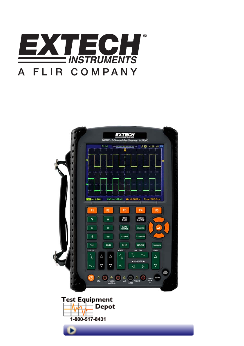
3.5 Observing a waveform
Press the AUTO button and a 1 KHz square wave of approx. 5V peak-to-peak will appear in the display.
Press the CH1 button and remove Channel 1. Move the Probe to the CH2 BNC, push the CH2 button
and repeat these steps to observe the test signal on Channel 2.
3.6 Probe Examination
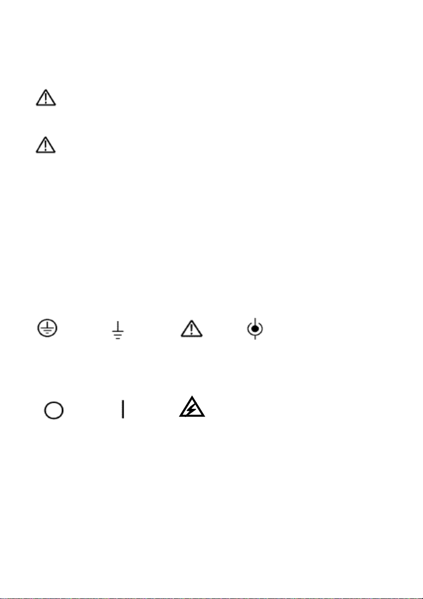
3.7 Safety
When using the probe, keep fingers behind the guard on the probe body to avoid electric shock. Do not
touch metallic portions of the probe head while it is connected to a voltage source. Connect the probe to
the oscilloscope and connect the ground terminal to ground before starting any measurements.
10 MS6000-EU-EN-V1.3 7/12
Page 11
3.8 Manual Probe Compensation
Upon the first connection of a probe to an input channel, manually perform this adjustment to match the
probe to the input channel. Uncompensated probes may lead to errors or faults in measurement.
To adjust the probe compensation, follow the steps below.
1. Set the switch on the probe to 10X and connect the probe to Channel 1 on the oscilloscope. Attach
the probe tip to the PROBE COMP ~5V@1KHz connector and the reference lead to the PROBE
COMP Ground connector. Press CH1 button and set the Probe attenuation to 10X. Press the
AUTO button and you should see the 1 KHz reference signal.
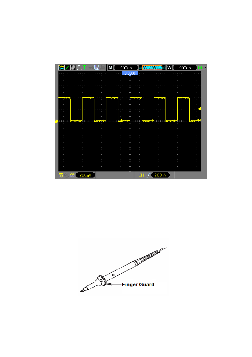
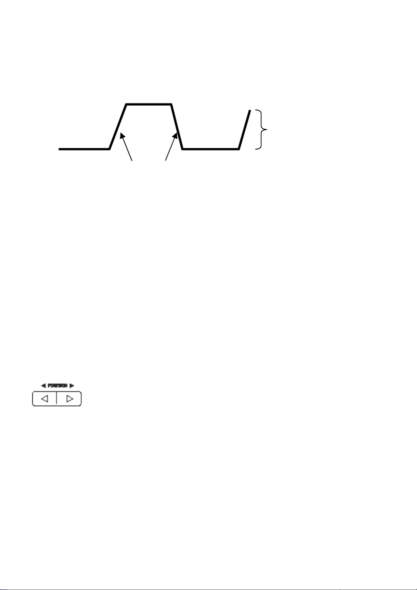
2. Check the shape of the displayed waveform.
Compensated correctly
Overcompensated
Undercompensated
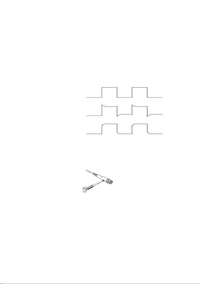
3. If necessary, use a nonmet allic screwdriver to adjust the variable probe capacitor until the shape of
the waveform appears to be the same as shown in the above figure. Repeat this step as necessary
for additional probes. Refer to the figure below for adjustment illustration.
11 MS6000-EU-EN-V1.3 7/12
Page 12
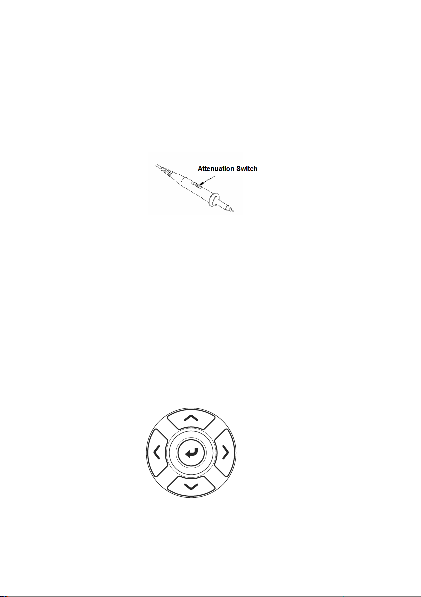
3.9 Probe Attenuation Setting
Probes are of various attenuation factors which affect the vertical scale of the signal. Ensure that the
attenuation switch on the probe matches the CH probe option in the oscilloscope. Switch settings are 1X
and 10X. T o set the probe attenuation to match the probe setting, push the vertical menu button (such as
the CH1 button) and select the probe option that matches the attenuation factor of the probe in use.
When the attenuation switch is set to 1X, the probe limits the bandwidth of the oscilloscope to 6MHz. To
use the full bandwidth of the oscilloscope, be sure to set the switch to 10X.
3.10 Self Calibration
The self calibration routine helps optimize the oscilloscope signal path for maximum measurement
accuracy. The routine can be run at any time but should always be run if the ambient temperature
changes by 5°C or more. For an accurate calibration, please power on the oscilloscope and wait 20
minutes before performing the Self calibration. To compensate the signal path, disconnect any probes
or cables from the front-panel input connectors.
3.11 Multifunction Control
The Multifunction Control arrows are used to move the cursors and change menu item settings.
12 MS6000-EU-EN-V1.3 7/12
Page 13

- Main Features
This chapter provides some general information the user should be aware of before using this
oscilloscope. It contains:
4.1 Oscilloscope setup
4.2 Trigger
4.3 Data Acquisition
4.4 Waveform scaling and positioning
4.5 Waveform measurement
3.12 Oscilloscope Setup
While operating the oscilloscope, the AUTOSET feature will, in most cases, be used.
Autoset: This function can be used to adjust the horizontal and vertical scales of the oscilloscope
automatically and set the trigger coupling, type, position, slope, level and mode, etc., to acquire a stable
waveform display. Press the AUTO button to engage Autoset.
3.13 Trigger
The trigger determines when the oscilloscope begins to acquire data and display a waveform. Once a
trigger is properly set up, the oscilloscope can convert unstable displays or blank screens to meaningful
waveforms. Basic information regarding triggering is provided below.
Trigger Source: The trigger can be generated from either CH1 or CH2. The input channel can trigger
normally whether or not the input signal is displayed.
Trigger Type: The oscilloscope has six types of triggers: Edge, Video, Pulse Width, Slope, Overtime,
and Alter. Press the TRIG button to engage this feature.
Edge Trigger Triggering occurs when the input trigger source crosses a specified level in a
specified direction.
Video Trigger performs a field or line trigger through standard video signals.
Pulse Width Trigger can trigger normal or abnormal pulses that meet trigger conditions.
Slope Trigger uses the rise and fall times on the edge of a signal for triggering.
Overtime Trigger occurs after the edge of a signal reaches the set time.
Alter Trigger uses a specific frequency to switch between two analog channels (CH1 and
CH2), so that the channels will generate swap trigger signals.
13 MS6000-EU-EN-V1.3 7/12
Page 14
g
j
y
Slope and Level: (Set Trig Type to Edge or Slope) The Slope and Level controls help to define the
trigger. The Slope option determines whether the trigger point is on the rising or falling edge of a signal.
To perform the trigger slope control, press the TRIG button and then select Edge trigger (F1), and use
the Slope button (F3) to select rising or falling. The LEVEL button controls where the trigger point is on
the edge.
Trigger level can be
usted verticall
ad
Rising Edge
Trigger slope can be rising or fallin
Trigger Mode: (Auto, Normal, Single) Select the Auto or Normal mode to define how the oscilloscope
acquires data when it does not detect a trigger condition. Aut o M od e performs the acquisition freely in
absence of valid trigger. It allows the generation of untriggered waveforms with the time base set to
80ms/div or slower. Normal Mode updates the displayed waveforms only when the oscilloscope detects
a valid trigger condition. Before this update, the oscilloscope continues to display the older waveforms.
This mode should be used when it is desired to only view the effectively triggered waveforms. In this
mode, the oscilloscope displays waveforms only after the first trigger.
Single mode will allow you to view a Single sweep of a waveform.
Trigger Coupling: (AC, DC, Noise Reject, HF Reject, LF Reject) Trigger Coupling determines which
part of the signal will be delivered to the trigger circuit. This can help to obtain a stable display of the
waveform. T o use trigger coupling, push the TRIG button, select Edge, Pulse, Slope, or O.T . trigger, and
then press F5 for page 2 and select a Coupling option.
Trigger Position: The horizontal position control establishes the time between the trigger position and
the screen center.
Falling Edge
14 MS6000-EU-EN-V1.3 7/12
Page 15

3.14 Data Acquisition
When an analog signal is acquired, the oscilloscope will convert it to a digital one. There are two kinds of
acquisitions: Real-time acquisition and Equivalent acquisition. The real-time acquisition has three
modes: Normal, Peak Detect, and Average. The acquisition rate is affected by the time base.
Real-Time Acquisition:
Normal: In this mode, the oscilloscope samples the signal in evenly spaced intervals to establish the
waveform. This mode accurately represents signals in most instances. However, it does not acquire
rapid variations in the analog signal that may occur between two samples, which can result in aliasing
and may cause narrow pulses to be missed. In such cases, use the Peak Detect mode to acquire data.
Peak Detect: In this mode, the oscilloscope obtains the maximum and minimum values of the input
signal over each sample interval and uses these values to display the waveform. In this way, the
oscilloscope can acquire and display narrow pulses that may have otherwise been missed in Normal
mode. However, noise will appear to be higher in this mode.
Average: In this mode, the oscilloscope acquires several waveforms, averages them, and displays the
resulting waveform. Use this mode to reduce random noise.
Equivalent Acquisition:
This type of acquisition can be utilized for periodic signals. In case the acquisition rate is too low when
using the real-time acquisition, the oscilloscope will use a fixed rate to acquire data with a stationary
(very small) delay after each acquisition of a frame of data. After repeating this acquisition for N times,
the oscilloscope will arrange the acquired N frames of data by time to make up a new frame of data; and
then the waveform can be recovered. The number of times (N) is related to the equivalent acquisition
rate.
Time Base: The oscilloscope digitizes waveforms by acquiring the value of an input signal at discrete
points. The time base helps to control how often the values are digitized. Use the TIME/DIV button to
adjust the time base to a horizontal scale that suits your requirements.
15 MS6000-EU-EN-V1.3 7/12
Page 16

3.15 Waveform Scaling and Positioning
The display of waveforms on the screen can be changed by adjusting their scale and position. Once the
scale changes, the waveform display will increase or decrease in size. Once the position changes, the
waveform will move up, down, right, or left.
The channel reference indicator (located on the left of the graticule) identifies each waveform on the
screen. It points to the ground level of the waveform record.
Vertical Scale and Position: The vertical position of a waveform can be changed by moving it up or
down on the screen. To compare data, align one waveform over another.
Horizontal Scale and Position: Pretrigger Information
The HORIZONTAL POSITION control can be adjusted to view waveform data before the trigger, after
the trigger, or some of each. When the horizontal position of a waveform is changed, the time between
the trigger position and the screen center is being changed.
For example, to find the cause of a glitch in a test circuit, trigger on the glitch and make the pre-trigger
period long enough to capture data before the glitch. Then analyze the pre-trigger data and perhaps find
the cause. Change the horizontal scale of all the waveforms by clicking the TIME/DIV button; for
example, to see just one cycle of a waveform to measure the overshoot on its rising edge. The
oscilloscope shows the horizontal scale as time per division in the scale readout. Since all active
waveforms use the same time base, the oscilloscope only displays one value for all of the active
channels.
16 MS6000-EU-EN-V1.3 7/12
Page 17
3.16 Waveform Measurement
The oscilloscope displays graphs of voltage versus time (YT) and can help to measure the displayed
waveform. There are several ways to take measurements, using the graticule, the cursors or performing
an automatic measurement.
Graticule: This method allows a quick, visual estimate and takes a simple measurement through the
graticule divisions and the scale factor.
For example, the user can take simple measurements by counting the major and minor graticule
divisions involved and multiplying by the scale factor. If 6 major vertical graticule divisions are counted
between the minimum and maximum values of a waveform and a scale factor of 50mV/division is
selected, the peak-to-peak voltage can be calculated as follows:
6 divisions x 50mV/division = 300mV.
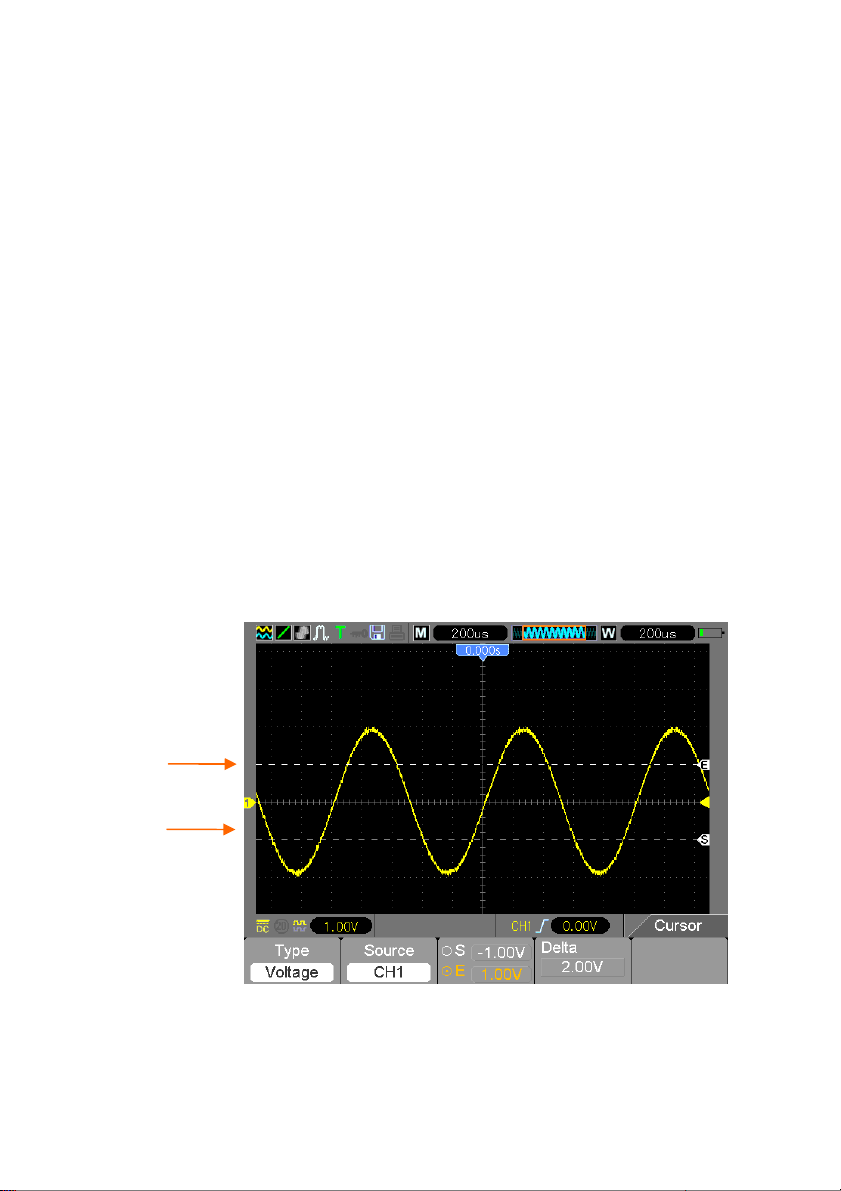
Cursor: This method allows the user to take measurements by moving the cursors. Cursors always
appear in pairs and the displayed readouts are just their measured values. There are two types of
cursors: Amplitude Cursor and Time Cursor. The amplitude cursor appears as a horizontal broken line,
measuring the vertical parameters. The time cursor appears as a vertical broken line, measuring the
horizontal parameters. When using the cursors please set the Source parameter to the desired
waveform. To use cursors, push the CURSOR button.
Cursor
Cursor
17 MS6000-EU-EN-V1.3 7/12
Page 18

Automatic Measurement: The oscilloscope performs all of the calculations automatically in this mode.
As this measurement uses the waveform record points, it is more precise than the graticule and cursor
measurements. Automatic measurements show the measurement results by readouts which are
periodically updated with the new data acquired by the oscilloscope. To use the Measurement mode
push the MEAS button.
18 MS6000-EU-EN-V1.3 7/12
Page 19
Chapter 4 - Basic Operation
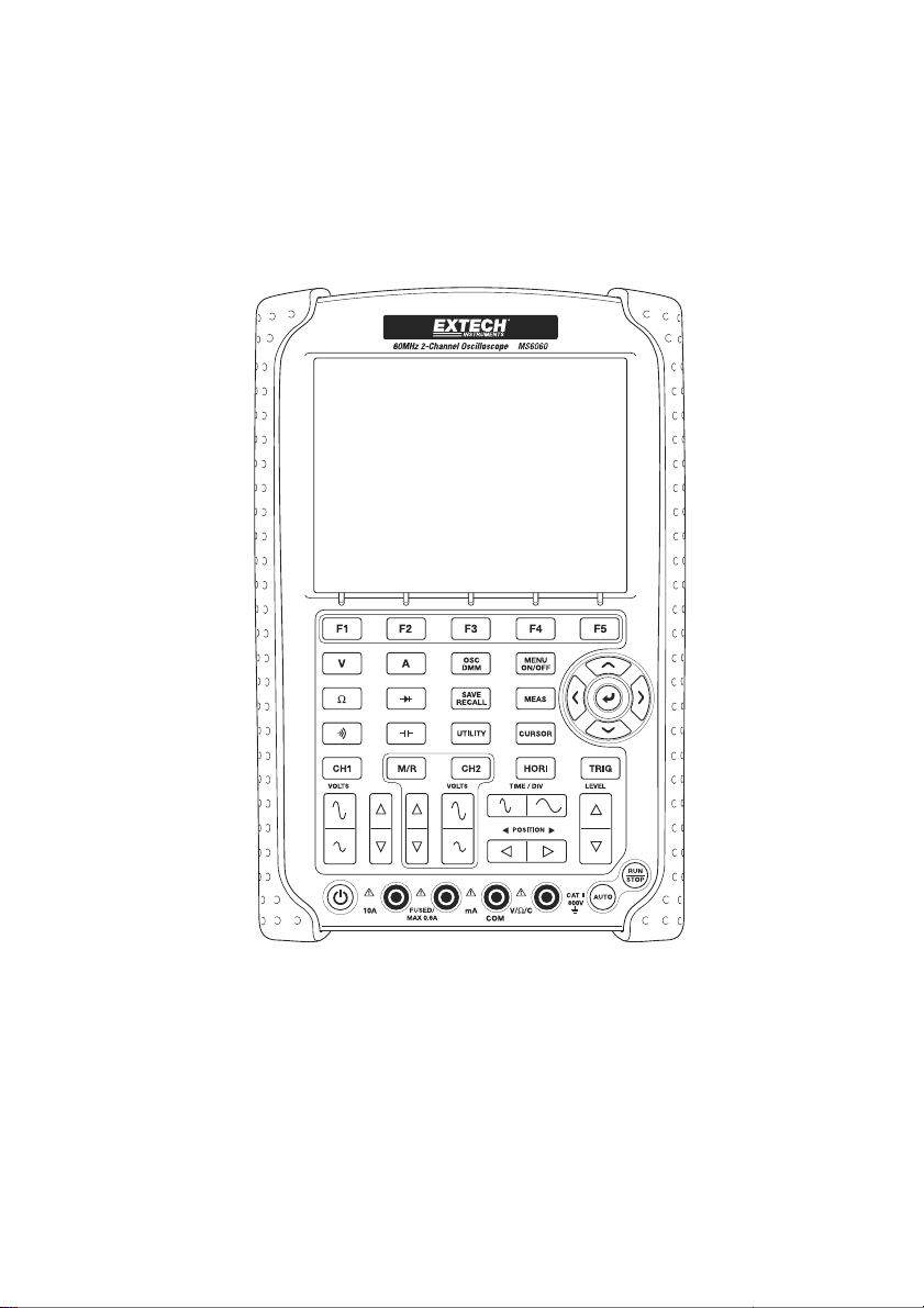
The front panel of the oscilloscope is divided into several functional areas. A quick overview of all control
buttons on the front panel as well as the displayed information on the screen and relative testing
operations is provided in this chapter. The figure below illustrates the front panel of the MS6000 series
digital oscilloscope.
Front Panel of the MS6000 Series
19 MS6000-EU-EN-V1.3 7/12
Page 20
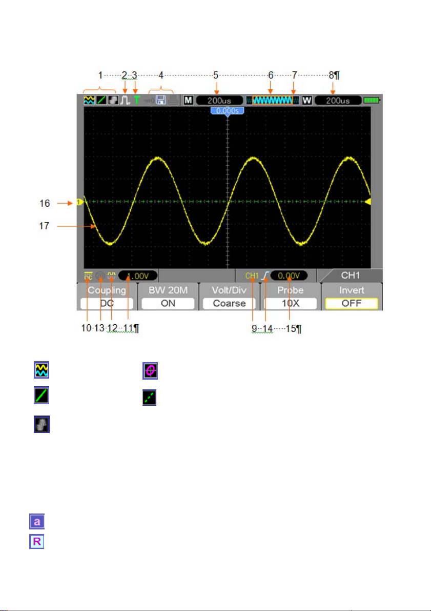
4.1 Display Area
1. Display Format:
: YT
: Vectors
:
Gray indicates auto persistence; Green indicates persistence display is
enabled. When the icon is set to green, the time for persistence display will be
shown behind it.
: XY
: Dots
2. Acquisition Mode: Normal, Peak Detect or Average
3. Trigger Status:
The oscilloscope is acquiring pre-triggered data.
All pre-triggered data have been acquired and the oscilloscope is ready to accept a trigger.
T The oscilloscope has detected a trigger and is acquiring the post-trigger information.
20 MS6000-EU-EN-V1.3 7/12
Page 21

The oscilloscope is in auto mode and is acquiring waveforms in the absence of triggers.
The oscilloscope is acquiring and displaying waveform data continuously in scan mode.
● The oscilloscope has stopped acquiring waveform data.
S The oscilloscope has finished a single sequence acquisition.
4. Tool Icon:
: If this icon appears, it indicates that the keyboard of the oscilloscope is locked by the host
computer via USB control.
: If this icon appears, it indicates that the USB disk has been connected.
: This icon lights up only when the USB slave interface is connected with the computer.
5. Readout shows the main time base setting.
6. Main Time Base Window
7. Display of window’s position in data memory and data length.
8. Window Time Base
9. Operating Menu shows information for the function keys.
10. Icon indicates channel coupling.
11. Level Range.
12. Icon indicates whether or not the waveform is inverted.
13. 20MB Bandwidth Limit. If this icon appears, it indicates that the bandwidth limit is enabled,
(otherwise the bandwidth limit is disabled).
14. Trigger Type:
: Edge trigger on the rising edge.
: Edge trigger on the falling edge.
: Video trigger with line synchronization.
: Video trigger with field synchronization.
: Pulse Width trigger, positive polarity.
: Pulse Width trigger, negative polarity.
15. Trigger Level.
16. Channel Marker
17. Window displays waveform.
21 MS6000-EU-EN-V1.3 7/12
Page 22

4.1.1 XY Format
The XY format is used to analyze phase differences, such as those represented by Lissajous patterns.
This format plots the voltage on CH1 against the voltage on CH2, where CH1 is the horizontal axis and
CH2 is the vertical axis. The oscilloscope uses the untriggered Normal acquisition mode and displays
data as dots. The sampling rate is fixed at 1 MS/s.
The oscilloscope can acquire waveforms in normal operation mode (YT format) at any sampling rate.
The same waveform can be displayed in XY format. To perform this operation, stop the acquisition and
change the display format to XY.
The table below covers several controls in XY format.
Controls Capability of XY format
CH1 VOLTS and VERTICAL POSITION controls Set the horizontal scale and position
CH2 VOLTS and VERTICAL POSITION controls
Reference or Math Unusable
Cursors Unusable
Auto (display format reset to normal operation - YT) Unusable
Time base controls Unusable
Trigger controls Unusable
Continuously set the vertical scale and
position
22 MS6000-EU-EN-V1.3 7/12
Page 23
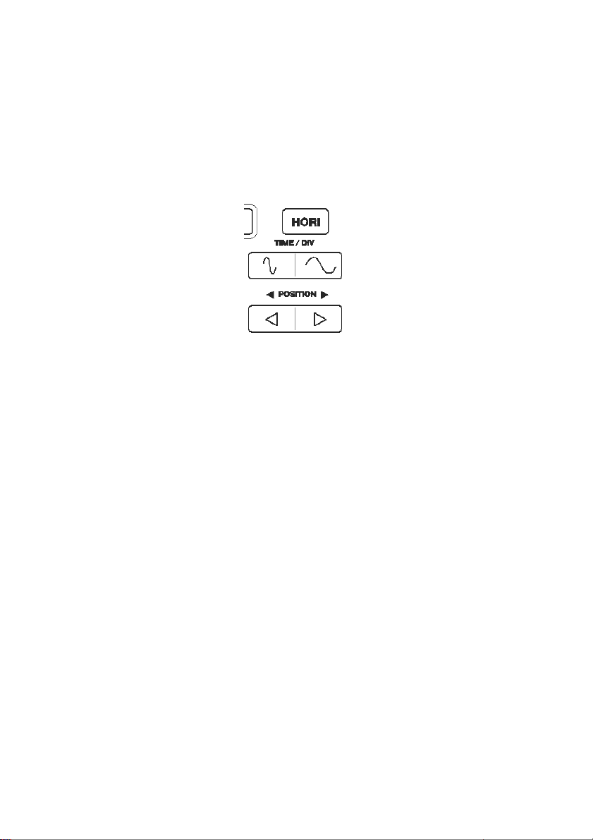
4.2 Horizontal Controls
Use the horizontal controls to change the horizontal scale and position of waveforms. The horizontal
position readout shows the time represented by the center of the screen, using the trigger time as zero.
When the horizontal scale is changed, the waveform will expand or contract to the screen center. The
readout near the upper right of the screen shows the current horizontal position in seconds.
M represents ‘Main Time Base’, and W indicates ‘Window Time Base’. The oscilloscope also has an
arrow icon at the top of the graticule to indicate the horizontal position.
1. HORIZONTAL POSITION BAR: Used to control the trigger position against the screen center.
2. TIME/DIV: Used to change the horizontal time scale so as to magnify or compress the waveform
horizontally . If the waveform acquisition is stopped (using the RUN/STOP button) the TIME /DIV control
will expand or compress the waveform. In dual-window mode, push button F1 to select major or minor
window. When the major window is selected, the F1 button provides the same functions as it provides in
single-mode window. When the minor window is selected, press TIME/DIV button to scale the waveform
(magnification can be set up to 1000x).
23 MS6000-EU-EN-V1.3 7/12
Page 24

3. Each option in HORI MENU is described as follows:
Options Settings Comments
Window Control (F1)
(Menu page 1)
Window Selection (F2)
(menu page 1)
Holdoff (F3)
(menu page 1)
Reset (F4)
(menu page 1)
Page (F5) Change Menu pages 1 to 3 when Window Control is set to
Double Window
Single Window
Major Window
Minor Window
Select this menu and click the up and down Arrow keys to
Selects either Single or Double window mode (see figures
below table). Press this option button in single-window
mode to enter the dual-window mode.
Selects the major (upper) or minor (lower) window in
dual-window mode. The window is highlighted once
selected.
adjust the trigger hold-off time within the range of
100ns-10s.
Double Window
Pre Mark (F2)
(menu page 2)
Next Mark (F3)
(menu page 2)
Set/Clear (F4)
(menu page 2)
Clear All (F2)
(menu page 3)
Play/Stop (F3)
(menu page 3)
Used when Marks are set in place. This button will position
the display to view the signal at any marks to the Left of your
present view.
Used when Marks are set in place. This button will position
the display to view the signal at any marks to the Right of
your present view.
Sets a mark or Clears the indicated mark. To place a Mark
on the signal, place that portion of the signal to be observed
at the center verticle line (Bottom window) using the
Horizontal Position button. Press the Set button to add or
remove that mark.
Clear all Marks
Push this button to auto move the signal from left to right.
Set the signal window to the left most position using the
Horizontal position button. Press Play to start the signal
moving across the screen. Press Stop to halt the
movement.
24 MS6000-EU-EN-V1.3 7/12
Page 25

Single-window Mode
Dual-window Mode
Location of expanded window data
Major Window
Minor Window
25 MS6000-EU-EN-V1.3 7/12
Page 26
4.2.1 Scan Mode Display (Roll Mode)
With the TIME/DIV control set to 80ms/div or slower and the trigger mode set to Auto, the oscilloscope
works in the scan acquisition mode. In this mode, the waveform display is updated from left to right
without any trigger or horizontal position control.
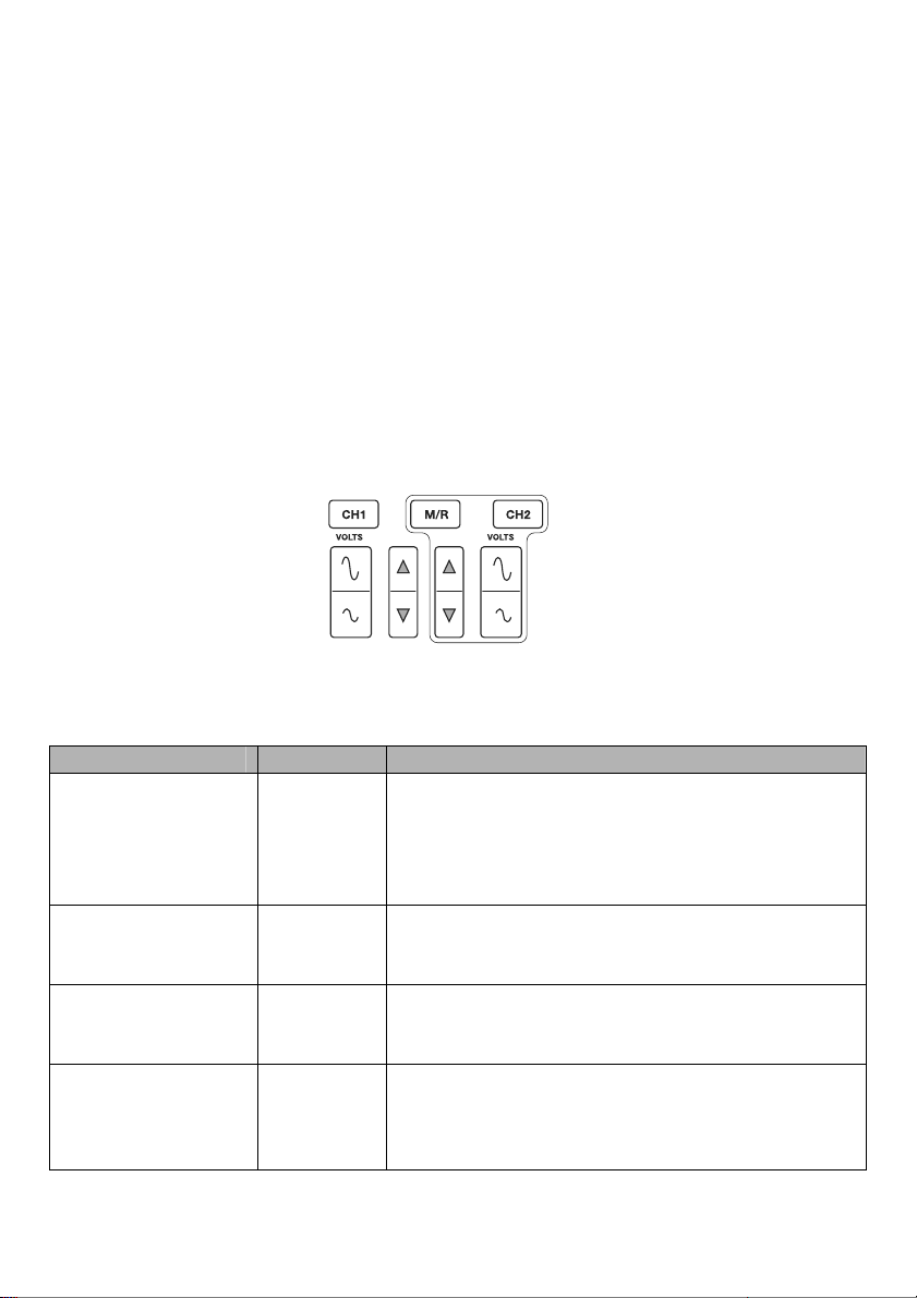
4.3 Vertical Controls
Vertical controls can be used to display and remove waveforms, adjust vertical size and position of the
signal, set input parameters and perform math calculations. Each channel has a separate vertical menu.
See below for menu description.
1. VERTICAL POSITION Bar: Move the channel waveform up and down on the screen. In
dual-window mode, move the waveforms in both windows at the same time in the same direction.
2. Menu (CH1, CH2): Display vertical menu options; turn ON or OFF the display of channel
waveforms. Press the MENU button to turn on the Menu. Press the CH1 or CH2 button to select
the channel you want to adjust. Press the F5 key to switch from Menu page 1 to page 2.
Options Settings Comments
DC passes both DC and AC components of the input signal.
Coupling (F1)
(menu page 1)
20MHz Bandwidth Limit
(F2)
(menu page 1)
VOLTS/Div (F3)
(menu page 1)
Probe Attenuation (F4)
(menu page 1)
DC
AC
Ground
OFF
ON
Coarse
Fine
1X
10X
100X
1000X
AC blocks the DC component of the input signal and
attenuates signals below 10Hz.
Ground disconnects the input signal and applies a zero volt
input.
Limits the bandwidth to reduce display noise; filters the
signal to eliminate noise and other unnecessary HF
components.
Selects the resolution of the VOLTS bar.
‘Coarse’ defines a 1-2-5 sequence. ‘Fine’ changes the
resolution in smaller steps between the Coarse settings.
Select a value to match the probe attenuation factor so as to
ensure correct vertical readouts. Reduce bandwidth to
6MHz when using a 1X probe.
26 MS6000-EU-EN-V1.3 7/12
Page 27

Invert (F2)
(menu page 2)
Reset (F3)
(menu page 2)
Ground Coupling
Ground Coupling is used to display a zero-volt waveform. Internally, the channel input is connected with
a zero-volt reference level.
Remove Waveform Display
T o remove a waveform from the screen, first push the menu button to display the vertical menu, and then
push the appropriate Channel button to remove the waveform. A channel waveform which is
unnecessary to display can be used as a trigger source or for math operations.
3. VOLTS
Control the oscilloscope to magnify or attenuate the source signal of the channel waveform. The vertical
size of the display on the screen will change (increase or decrease). The key F3 may be used to switch
between Coarse and Fine. In the Fine resolution setting, the vertical scale readout displays the actual
VOLTS setting. The vertical scale changes only when the control is set to Course and the VOL TS control
is adjusted.
Off
On
Resets Vertical settings to default
Inverts the waveform relative to the reference level.
27 MS6000-EU-EN-V1.3 7/12
Page 28

4. MATH MENU: Display the waveform math operations. See the table below for details.
The MATH menu contains source options for all math operations. Press the M/R button.
Operations Source Options Comments
Enable (F1)
Operate (F2)
FFT (F2)
Note: All selected menus are highlighted orange.
ON
OFF
CH1+CH2 Add Channel 1 to Channel 2.
CH1-CH2
CH2-CH1
CH1xCH2 Multiply CH1 with CH2
CH1/CH2 Divide CH1 by CH2
CH2/CH1 Divide CH2 by CH1
Source(F3)
CH1 or CH2
ON enables the Math functions
Subtract the Channel 2 waveform from the Channel
1 waveform.
Subtract the Channel 1 waveform from the Channel
2 waveform.
WINDOW (F4) – There are 5 types of window
settings available: Hanning, Flattop, Rectangular,
Bartlett, and Blackman
Zoom (F2 page 2): Use the FFT Zoom button to
adjust the window size.
Scale: x1, x2, x5, x10.
Vertical Base (F3 page 2): dBrms or Vrms
28 MS6000-EU-EN-V1.3 7/12
Page 29

4.3.1 Math FFT
This chapter elaborates on the Math FFT (Fast Fourier Transform) functionality. The Math FFT mode
may be used to convert a normal time-domain (YT) signal to its frequency components (spectrum), and
to observe the following:
Analyze harmonics in power cords;
Measure harmonic content and distortion in systems;
Characterize noise in DC power supplies;
Test impulse response of filters and systems;
Analyze vibration.
To use the Math FFT mode, perform the following tasks:
Set the source (time-domain) waveform;
Display the FFT spectrum;
Choose a type of FFT window;
Adjust the sample rate to display the fundamental frequency and harmonics without aliasing;
Use zoom controls to magnify the spectrum;
Use cursors to measure the spectrum.
4.3.1.1 Setting Time-domain Waveform
It is necessary to set the normal time-domain (YT) waveform before using the FFT mode. Follow the
steps below:
1. Push the AUTO button to display a standard YT waveform.
2. Click the VOLTS Key to ensure the entire waveform is visible on the screen. If the waveform is
invisible, the oscilloscope may display erroneous FFT results by adding high-frequency
components.
3. Click the Vertical Position key to vertically move the YT waveform to the center (zero division) so as
to ensure the FFT will display a true DC value.
4. Click the Horizontal Position key to position the part of the YT waveform to be analyzed in the
center eight divisions of the screen. The oscilloscope uses the 2048 center points of the
time-domain waveform to calculate the FFT spectrum.
5. Click the TIME/DIV key to provide the resolution needed in the FFT spectrum.
If possible, set the oscilloscope to display multiple signal cycles. If the TIME/DIV key is clicked to
select a faster setting (fewer cycles), the FFT spectrum will display a larger frequency range and
reduce the possibility of FFT aliasing.
29 MS6000-EU-EN-V1.3 7/12
Page 30

6. To set the FFT display, follow the steps below:
1. Push the M/R button;
2. Set the Operate key (F2) to FFT;
3. Select the Math FFT Source (F3) channel.
In many situations, the oscilloscope can also generate a useful FFT spectrum despite the YT waveform
not being triggered. This is true if the signal is periodic or random (such as noise).
Note: Trigger and position transient or burst waveforms as close as possi ble to the screen
center.
Nyquist Frequency
The highest frequency that any real-time digital oscilloscope can measure without errors is half of the
sample rate, which is called the Nyquist frequency. Frequency information beyond the Nyquist
frequency is under sampled which brings about the FFT aliasing. The math function can convert the
center 2048 points of the time-domain waveform to an FFT spectrum. The resulting FFT spectrum
contains 1024 points from DC (0Hz) to the Nyquist frequency. Usually, the screen compresses the FFT
spectrum horizontally to 250 points, but you can use the FFT Zoom function to expand the FFT spectrum
so that you can clearly view the frequency components at each of the 1024 data points in the FFT
spectrum.
Note: The oscilloscope’s vertical response is slightly larger than its bandwidth (60MHz, 100MHz
or 200MHz, depending on the model; or 20MHz when the Bandwidth Limit option is set to
Limited). Therefore, the FFT spectrum can display valid frequency information above the
oscilloscope bandwidth. However, the amplitude information near or above the bandwidth wil l
not be accurate.
30 MS6000-EU-EN-V1.3 7/12
Page 31

4.3.1.2 Displaying FFT Spectrum
Push the MATH (M/R) button to display the Math menu. Use the options to select the Source channel,
the Window algorithm, and the FFT Zoom factor. Only one FFT spectrum can be displayed at a time.
Math FFT Options Settings Comments
Source (F3)
(menu page 1)
Window (F4)
(menu page 1)
FFT Zoom (F2)
(Menu page 2)
Refer to image above for the following:
1. Frequency at the center graticule line
2. Vertical scale in dB per division (0dB=1V
3. Horizontal scale in frequency per division
4. Sample rate in number of samples per second
5. FFT Window type is set to desired type.
CH1, CH2 Choose a channel to be the FFT source.
Hanning, Flat Top,
Rectangular(None),
Bartlett, Blackman
X1, X2, X5, X10
Select a type for the FFT window. For more
information, refer to Section 5.3.1.3.
Change the horizontal magnification of the FFT
display. For detailed information, refer to Section
5.3.1.6.
(Math menu page 2 – F3))
RMS,
31 MS6000-EU-EN-V1.3 7/12
Page 32
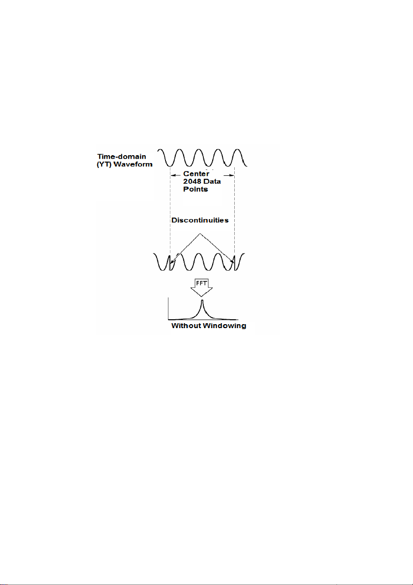
4.3.1.3 Selecting FFT Window
Using FFT windows can eliminate the spectral leakage in the FFT spectrum. The FFT algorithm
assumes that the YT waveform repeats all the time. When the number of cycles is integral (1, 2, 3 ...),
the YT waveform starts and ends at the same amplitude and there are no discontinuities in the signal
shape.
If the number of cycles is non-integral, the YT waveform starts and ends at different amplitudes and the
transitions between the start and end points will cause discontinuities in the signal that introduce
high-frequency transients.
32 MS6000-EU-EN-V1.3 7/12
Page 33
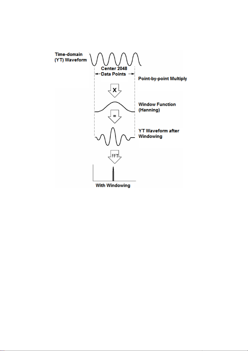
Applying a FFT window to the YT waveform changes the waveform so that the start and stop values are
close to each other, thereby reducing the discontinuities. (Figure - Hanning window).
33 MS6000-EU-EN-V1.3 7/12
Page 34

FFT Window Selection: The Math FFT function has Five FFT Window options. There is a trade-off
between frequency resolution, Spectral Leakage, and amplitude accuracy for each type of the window
choices. Determine which one to choose according to the desired object to be measured and the source
signal characteristics.
Window Measurement Characteristics
Hanning Random Waveform
Flat Top
Rectangular
(None or Boxcar)
Bartlett Random Waveform
Blackman
Sinusoid
Waveform
Pulse or Transient
Waveform
Random or Mixed
Waveform
Good frequency resolution, Fair amplitude accuracy, and
Good Spectral leakage.
Poor frequency resolution, Best amplitude accuracy, and
Good Spectral Leakage.
Special-purpose window applicable to discontinuous
waveforms. Best frequency resolution, Poor amplitude
accuracy, and Poor Spectral Leakage.
Good frequency resolution, Fair amplitude accuracy, and
Fair Spectral Leakage.
Poor frequency resolution, Best amplitude accuracy, and
Best Spectral Leakage.
4.3.1.4 FFT Aliasing
Problems occur when the time-domain waveform acquired by the oscilloscope contains frequency
components higher than the Nyquist frequency. The frequency components above the Nyquist
frequency will be under sampled and displayed as lower frequency components that ‘fold back’ from the
Nyquist frequency. These erroneous components are called aliases.
4.3.1.5 Eliminating Aliases
To eliminate aliases, use the following methods.
Click the TIME/DIV key to set a faster sample rate. Since the Nyquist frequency increases as the
sample rate is increased, the aliased frequency components will be displayed correct. If too many
frequency components appear on the screen, use the FFT Zoom option to magnify the FFT
spectrum.
If there is no need to observe the frequency components above 20MHz, set the CH Bandwidth
Limit option to Limited.
Filter the signal input and limit the bandwidth of the source waveform to lower than the Nyquist
frequency.
Identify and ignore the aliased frequencies.
Use zoom controls and cursors to magnify and measure the FFT spectrum.
34 MS6000-EU-EN-V1.3 7/12
Page 35

4.3.1.6 Magnifying and Positioning FFT Spectrum
The FFT spectrum may be scaled, and the cursors used, to measure through the FFT Zoom option
which enables horizontal magnification. To vertically magnify the spectrum, use the vertical controls.
Horizontal Zoom and Position
The FFT Zoom option (page 2 of FFT option) may be used to magnify the FFT spectrum horizontally
without changing the sample rate. The available zoom factors are X1 (default), X2, X5 and X10. When
the zoom factor is set to X1 and the waveform is located at the center graticule, the left graticule line
position is 0Hz and the right position is the Nyquist frequency.
The FFT spectrum is magnified to the center graticule line when the zoom factor is adjusted. That is, the
axis for horizontal magnification is the center graticule line. Click the Horizontal Position Key to move the
FFT spectrum to the right.
Vertical Zoom and Position
When the FFT spectrum is being displayed, the channel vertical keys become the zoom and position
controls corresponding to their respective channels. The VOLTS key provides the following zoom
factors: X1 (default), X2, X5 and X10. The FFT spectrum is magnified vertically to the marker M (math
waveform reference point on the left edge of the screen). Click the Vertical Position key to move the
spectrum upward.
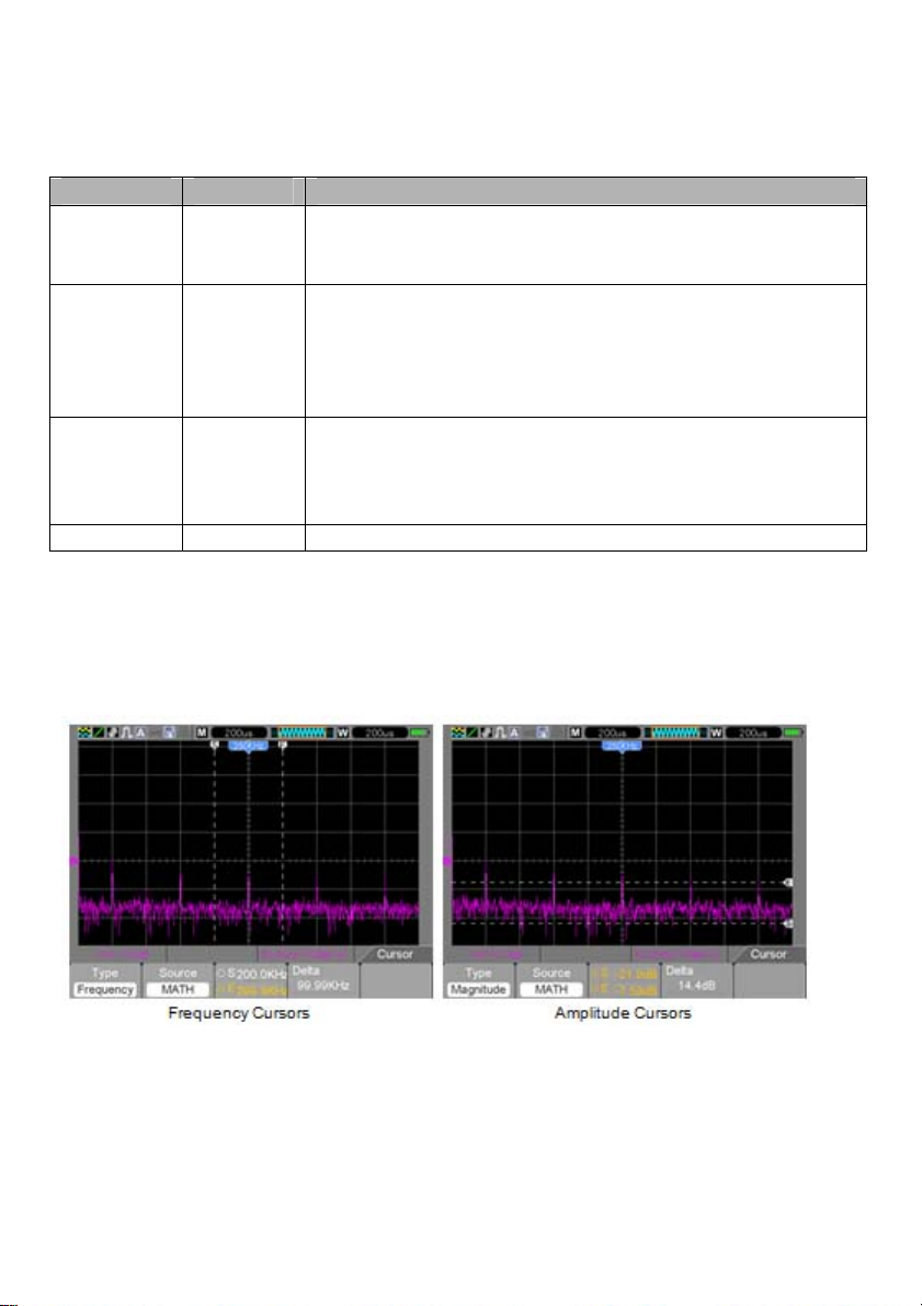
4.3.1.7 Using Cursors to Measure FFT Spectrum
Cursors may be used to take two measurements on the FFT spectrum: amplitude (in dB) and frequency
(in Hz). Amplitude is referenced to 0db equaling 1VRMS. Use cursors to measure at any zoom factor as
desired.
Push the CURSOR button and if the Type option is OFF select Volt age or Time. Click the Source option
and select Math. Press the Type option button to select between Voltage or Frequency. Click the
SELECT CURSOR option (F3) to choose a cursor, S or E. When highlighted move Cursor S and Cursor
E. Use the horizontal cursor to measure the amplitude and the vertical cursor to measure the
frequency. Now the display at the DELTA menu is just the measured value, and the values at Cursor S
and Cursor E. Delta is the absolute value of Cursor S minus Cursor E.
35 MS6000-EU-EN-V1.3 7/12
Page 36

36 MS6000-EU-EN-V1.3 7/12
Page 37

4.4 Trigger Controls
The trigger can be defined through the Trigger Menu. There are six types of triggering: Edge, Video,
Pulse Width, Swap, Slope and Overtime. Refer to the following tables to view the options for each type
of trigger.
TRIG MENU
Push the TRIG button to display trigger menus. The edge trigger is most commonly used. See the table
below for details.
Options Settings Comments
Type (F1)
Source
(F2)
Slope (F3)
Edge, Video,
Pulse, Slope,
and Overtime
CH1
CH2
Rising
Falling
By default the oscilloscope uses the edge trigger which triggers the
oscilloscope on the rising or falling edge of the input signal when it
crosses the trigger level (threshold).
Select the input source as the trigger signal.
CH1, CH2: Whether or not the waveform is displayed, the channel will
be triggered.
When Type (F1 ) is set to Edge, Set the edge to trigger for rising or
falling
When Type (F1) is set to Edge, Slope, Pulse, and OT select a trigger
mode.
Mode (F4)
Auto
Normal
Single
Auto mode (default): In this mode, the oscilloscope is forced to
trigger when it does not detect a trigger within a certain amount of time
based on the TIME/DIV setting. The oscilloscope goes into the scan
mode at 80ms/div (or slower) time base settings.
Normal mode: the oscilloscope updates the display only when it
detects a valid trigger condition. New waveforms are not displayed
until they replace older ones. Use this mode to just view valid
triggered waveforms (the display appears only after the first trigger
occurs).
Single mode: This mode will allow you to view a Single sweep of a
waveform.
37 MS6000-EU-EN-V1.3 7/12
Page 38

AC: Blocks DC components and attenuates signals below 10Hz.
AC
Coupling
(menu
page 2)
NOTE: Trigger coupling only affects the signal passed through the trigger system. It do es not
affect the bandwidth or coupling of the signal displayed on the screen.
Video Trigger
Options Settings Comments
Video (F1) None
Source (F2)
Polarity (F3)
Standard (F4) NTSC
Sync (F5)
Note: With ‘Normal Polarity’, the trigger always occurs on negative-going s ync pulses. If the
video signal contains positive-going sync pulses, use the Inverted Polarity option.
DC
HF Reject
LF Reject
Noise Reject
Pal/SECAM
Line Number
DC: Passes all components of the signal to the trigger circuit.
HF Reject: Attenuates the high-frequency components above 80kHz.
LF Reject: Blocks DC components and attenuates the low-frequency
components below 8kHz. Rejects power-line hum.
Noise Reject: S
imilar to DC coupling, except the sensitivity is
reduced to minimize false triggering on very noisy signals.
With Video highlighted, an NTSC, PAL or SECAM standard
video signal will be triggered. The trigger coupling is preset
to AC.
CH1
CH2
Normal
Inverted
All Lines
Odd Field
Even Field
All Fields
Select the input source as the trigger signal.
Normal: Triggers on the negative edge of the sync pulse.
Inverted: Triggers on the positive edge of the sync pulse.
Choose a proper video sync. When selecting Line Number
for the Sync option, use the User Select option to specify a
line number.
38 MS6000-EU-EN-V1.3 7/12
Page 39

Pulse Width Trigger
Use to trigger on aberrant or abnormal pulses.
Options Settings Comments
Pulse (F1)
(menu page 1)
Source (F2)
(menu page 1)
Polarity (F3)
(menu page 1)
Mode (F4)
(menu page 1)
Coupling (F2)
(menu page 2)
CH1
CH2
Positive
Negative
Auto
Normal
Single
DC
AC
HF Reject
LF Reject
Noise Reject
=
When (F3)
(menu page 2)
PulseWidth (F4)
(menu page 2)
F5 Switch between submenu pages
≠
>
<
20ns to 10.0sec With Set Pulse Width highlighted, set the pulse width.
With Pulse highlighted, the trigger occurs on pulses that meet
the trigger condition (defined by the ‘Source’, ‘When’ and ‘Set
Pulse Width’ options).
Select the input source as the trigger signal.
Polarity
Select the type of trigger. The Normal mode is best for most
pulse width trigger applications.
Select the component of the trigger signal applied to the
trigger circuit.
HF Reject: Attenuates the high-frequency components above
80kHz.
LF Reject: Blocks DC components and attenuates the
low-frequency components below 8kHz.
Noise Reject: S
imilar to DC coupling, except the
sensitivity is reduced to minimize false triggering
on very noisy signals.
Select the trigger condition.
39 MS6000-EU-EN-V1.3 7/12
Page 40
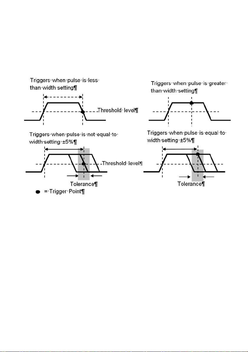
Trigger “When”: The pulse width of the source must be ≥5ns so that the oscilloscope can detect the
pulse.
, ≠: Within a ±5% tolerance, triggers the oscilloscope when the signal pulse width is equal to or not
equal to the specified pulse width.
, : Triggers the oscilloscope when the source signal pulse width is less than or greater than the
specified pulse width.
40 MS6000-EU-EN-V1.3 7/12
Page 41

Slope Trigger: Judges trigger according to the rising or falling time (more flexible and accurate than the
Edge trigger).
Options Settings Comments
Slope (F1) Choose which slope the signal is triggered from.
Source (F2)
Slope (F3)
Mode (F4)
Coupling (F2)
(menu page 2)
Vertical (F3)
(menu page 2)
When (F4)
(menu page 2)
Time (F2)
(menu page 3)
CH1
CH2
Rising
Falling
Normal
Auto
Single
DC
AC
Noise Reject
HF Reject
LF Reject
V1
V2
=
≠
>
<
20ns to 10.0sec
Select the input source as the trigger signal.
Select which slope of the signal is triggered on.
Select the type of trigger. The Normal mode is best for
most applications.
Selects the components of the trigger signal applied to the
trigger circuitry.
Adjust the vertical window by setting two trigger levels.
Select the trigger condition.
With this option highlighted, set the time span using the
multifunction control.
41 MS6000-EU-EN-V1.3 7/12
Page 42

Alter Trigger: (A feature of analog oscilloscopes) provides stable displays of signals at two different
frequencies. Mainly it uses a specific frequency to switch between two analog channels CH1 and CH2
so that the channels will generate swap trigger signals through the trigger circuitry.
Options Settings Comments
Alter (F1)
Press CH1 (F2) or CH2 (F3)
Must be in Single Window mode (HORZ)
Channel
Options in submenus. Alter (Swap) Trigger allows CH1 and CH2 to select trigger modes and to display
waveforms on the same screen. That is, both channels can choose from the four trigger modes.
Type Edge
Slope (F2)
Coupling (F3)
Back (F4) Displays initial Alter mode Trigger screen to allow CH selection
Type Video
Polarity (F2)
Standard (F3)
Sync (F4)
Back (F5) Displays initial Alter mode Trigger screen to allow CH selection
CH1 (F2)
CH2 (F3)
Rising
Falling
AC
DC
HF Reject
LF Reject
Noise Reject
Normal
Inverted
NTSC
PAL/SECAM
All Lines
All Fields
Even Field
Odd Field
Line Number
Push an option such as CH1, select the channel trigger type and
set the menu interface.
Select which slope of the signal is triggered on.
Select the components of the trigger signal applied to the trigger
circuitry.
Select to trigger on positive or negative pulses.
42 MS6000-EU-EN-V1.3 7/12
Page 43

Type Pulse
Polarity (F2)
When (F3)
Set PW (F4) Pulse Width Use Multifunction control to set Pulse width.
Page (F5) Set Menu page to 1 or 2
Coupling (F2)
Back (F3) Displays initial Alter mode Trigger screen to allow CH selection
Type O.T.
Polarity (F2)
Overtime (F3) Use Multifunction control to set Overtime timing.
Coupling (F4)
Back (F5) Displays initial Alter mode Trigger screen to allow CH selection
Positive
Negative
=
≠
<
>
AC
DC
HF Reject
LF Reject
Noise Reject
Positive
Negative
AC
DC
HF Reject
LF Reject
Noise Reject
Select to trigger on positive or negative pulses.
Select the trigger condition.
Select the components of the trigger signal applied to the trigger
circuitry.
Select to trigger on positive or negative pulses.
Selects the components of the trigger signal applied to the
trigger circuitry.
43 MS6000-EU-EN-V1.3 7/12
Page 44

Overtime Trigger: In Pulse Width trigger mode, it may take some time for a trigger to occur. Since a
complete pulse width is not needed to trigger the oscilloscope, it may be desired to trigger just upon the
overtime point. This is called Overtime Trigger. Press on TRIG to enter Trigger mode.
Options Settings Comments
Type O.T.
Source (F2)
Polarity (F3)
Mode (F4)
Page (F5) Change page from 1 to 2
Overtime (F2)
(menu page 2)
Coupling (F3)
(menu page 2)
50% (F4)
Page (F5) Change page from 2 to 1
CH1
CH2
Positive
Negative
Normal
Auto
Single
Adjust timing using the Multifunction control.
AC
DC
HF Reject
LF Reject
Noise Reject
Select channel to source the trigger
Select to trigger on positive or negative pulses.
Select the type of trigger. The Normal mode is best for most
applications.
Selects the components of the trigger signal applied to the
trigger circuitry.
44 MS6000-EU-EN-V1.3 7/12
Page 45

f
f
A
A
Holdoff: T o use T rigger Holdoff, push the HORI button and set the Holdoff Time option (F3). The Trigger
Holdoff function can be used to generate a stable display of complex waveforms (such as pulse trains).
Holdoff is the time between when the oscilloscope detects one trigger and when it is ready to detect
another. During the holdoff time, the oscilloscope will not trigger. For a pulse train, the holdoff time can
be adjusted to let the oscilloscope trigger only on the first pulse in the train.
Use the Multifunction control to adjust the timing for this feature.
Trigger Level
Indicates
Trigger Points
cquisition Interval
Holdof
cquisition Interval
Holdof
45 MS6000-EU-EN-V1.3 7/12
Page 46

4.5 Menu and Option Buttons
As shown below, these four buttons on the front panel are used mainly to recall relative setup menus.
SAVE/RECALL: Displays the Save/Recall menu for setups and waveforms. (Save/Recall)
MEASURE: Displays the Measure menu. (MEAS)
CURSOR: Displays the Cursor menu. (CUSOR )
UTIILITY: Displays the Utility menu. (UTILITY)
DISPLAY: Displays the Display menu. Click Utility button and go to menu page 4, Display is F3.
ACQUIRE: Displays the Acquire menu. Click Utility button and go to menu page 4, Acquire is F4.
4.5.1 SAVE/RECALL
Press the SAVE/RECALL button to save or recall oscilloscope setups or waveforms.
The first page shows the following menu.
Options Settings Comments
Wave F1 Press F1 to engage Waveform mode
Source (F1)
Media (F2)
Location (F3) Used with SD and Flash only. Select the memory location
Save (F4) Save the current set up
Page (F5) Change page from 1 to 2
Recall (F2)
(menu page 2)
Delete (f3)
(menu page 2)
CH1
CH2
SD
USB
Flash
Recall a specified setup based on the memory and location.
Delete a specified setup based on the memory and location.
Select a waveform display to store.
Select the location for saving the data
46 MS6000-EU-EN-V1.3 7/12
Page 47

Press the Save/Recall button to view the Save/Recall main menu.
Options Settings Comments
SetUp (F2) From the main Setup/Recall menu, Press F2 to engage SetUp mode
Source (F1)
Location (F2) 0 to 9
Save (F3) Complete the saving operation.
Recall (F4)
Back (F5) Returns you to the Save/Recall main menu
Options Settings Comments
CSV (F3) From the main Setup/Recall menu, Press F3 to engage CSV mode
Source (F1)
File List (F2)
Save (F3) Complete the saving operation.
Recall (F4)
Delete (F5) Delete the highlighted waveform file from the USB device.
See below for waveform menus.
Local
USB
CH1
CH2
Close
Open
Store the current setups to the USB disk or the Local internal memory
of the oscilloscope.
Specify the memory location in which to store the current waveform
settings or from which to recall the waveform settings.
Recall the oscilloscope settings stored in the location selected in the
Setup field.
Select a waveform display to store.
Open a file to save the waveform in. A USB device must be
connected in order to save the waveform. Close file after saving.
Recall the oscilloscope waveform stored in the location selected in the
Setup field. USB device must be attached and contain saved file
At most 9 groups of setups can be stored
Note: The oscilloscope will save the current settings 5 seconds after the last modification, and it
will recall these settings the next time the oscilloscope is powered ON.
The white waveforms on the menu is the
recall RefA waveform
47 MS6000-EU-EN-V1.3 7/12
Page 48

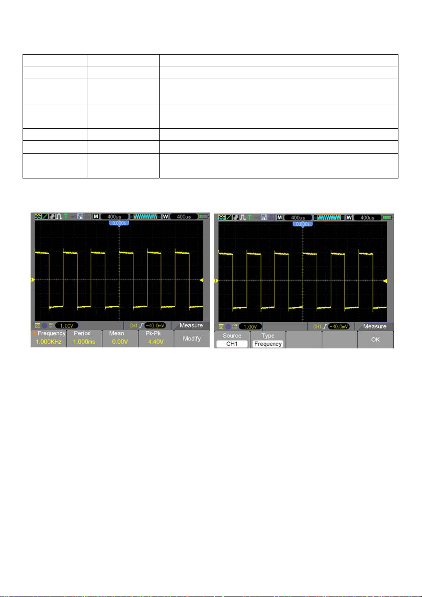
4.5.2 MEASURE
Push the MEAS key to view the following menu.
There are 23 types of measurements and up to 8 can be displayed at a time.
Options Settings Comments
Modify (F5) Press F5 to Select the measure Source and Type.
Source (F1)
Type (F2) Frequency Calculate the waveform frequency by measuring the first cycle.
Period Calculate the time of the first cycle.
Average/Mean Calculate the arithmetic mean voltage over the entire record.
Pk-Pk
CRMS
Minimum
Maximum
Rising
Falling
+ Width
- Width
Delay 1-2 ↑ The delay of the rising time between Channel 1 and Channel 2
Delay 1-2 ↓ The delay of the falling time between Channel 1 and Channel 2
+ Duty
- Duty
Base
Top
CH1
CH2
Select the measure source.
Calculate the absolute difference between the greatest and the
smallest peaks of the entire waveform.
Calculate the actual RMS voltage measurement of the first
complete cycle of the waveform.
Examine the waveform record of all points in the current window
and display the minimum value.
Examine the waveform record of all points in the current window
and display the maximum value.
Measure the time between 10% and 90% of the first rising edge
of the waveform.
Measure the time between 90% and 10% of the first falling edge
of the waveform.
Measure the time between the first rising edge and the next
falling edge at the waveform 50% level.
Measure the time between the first falling edge and the next
rising edge at the waveform 50% level.
Positive duty cycle =(Positive pulse width)/Period x 100%.
Measured from the first waveform.
Negative duty cycle =(Negative pulse width)/Period x 100%.
Measured from the first waveform.
Voltage of the st atistical minimum level, measured over the entire
waveform
Voltage of the statistical maximum level, measured over the
entire waveform
48 MS6000-EU-EN-V1.3 7/12
Page 49
Middle Voltage at the 50% level of the base to the top
Amplitude Amplitude = Base – Top, measured over the entire waveform
Overshoot
Preshoot
RMS The Root Mean Square voltage over the entire waveform
Off Do not take a measurement.
OK (F5)
Negative overshoot = (Base – Min)/Amp x100%, measured over
the entire waveform
Postitive overshoot = (Max – Top)/Amp x100%, measured over
the entire waveform
Press to engage Measurement after Source and Type is
selected.
The readouts in larger font size on the menu are the results of the corresponding measurements
only.
Taking Measurements: For a single waveform (or a waveform divided among multiple waveforms), up
to 8 automatic measurements can be displayed at a time. The waveform channel must stay in an ‘ON’
(displayed) state to facilitate the measurement. The automatic measurement cannot be performed on
reference or math waveforms, or in XY or Scan mode.
49 MS6000-EU-EN-V1.3 7/12
Page 50
4.5.3 CURSOR
The Cursor Menu is accessed by pressing the CURSOR button.
Options Settings Comments
Off
Type (F1)
Source (F2)
Select Cursor
(F3)
Delta (F4) Displays the measurement of the difference between the two cursors.
Moving Cursors: Press the Select Cursor (F3) key to select a cursor (S, E, or both) and move it using
the multifunction control. Cursors can be moved only when the Cursor Menu is displayed.
Voltage
Time
CH1
CH2
MATH
REFA
REFB
S
E
Select a measurement cursor and display it.
Voltage measures amplitude while Time measures frequency and
time.
Select a waveform to take the cursor measurement.
Use the readouts to show the measurement.
‘S’ indicates Cursor 1. ‘E’ indicates Cursor 2.
A selected cursor can be moved independently using the Multifunction
ring control. When neither cursor is highlighted, they both are moved
at the same time using the arrow keys on the Multifunction control.
50 MS6000-EU-EN-V1.3 7/12
Page 51

4.5.4 UTILITY
Push the UTILITY button to display the Utility Menu as follows.
Options Comments
Sys Info (F1)
(menu page 1)
Update (F2)
(menu page 1)
Self Cal* (F3)
(menu page 1)
System (F2)
(menu page 2)
Shutdown (F3)
(menu page 2)
Video (F4)
(menu page 2)
Display the software and hardware versions, serial number and other information
about the oscilloscope.
Insert a USB disk with an upgrade program; the disk icon at the top left corner is
highlighted. Press F4 to Confirm the Update Program button; the Software Upgrade
dialog will pop up. Press F2 (Highlighted Update) to cancel operation.
Press this option and the Self Calibration dialog will pop up. Press F4 to Confirm and
perform the self calibration. Press F3 (Highlighted Self Cal) to cancel. Remove all
probes before test.
Set System parameters. Sound (On/Off), Language (English, Chinese), Interface
color, Time Set (Date and Time), PC Set (USB or NET).
Set the meters Auto-Off timing when Action is set to PowerOff. Set Auto-Off time (F2)
using the Multifunction control arrow keys. Press F3 to confirm setting changes,
Press F4 to cancel changes, Press F5 to go back to main Utility menu.
Record a video of your waveforms.
Play
USB to SD
SD to USB
Delete
Back – go back to the main Utility menu
Probe Ck (F2)
(menu page 3)
Probe Check
Probe - (CH-1x, CH2-1x, CH1-10x, CH2-10x) Set to match probe setting.
Check - Turn on 1KHz Comp signal
Finish - Turn off Comp signal
Cancel - Cancel Probe Check
51 MS6000-EU-EN-V1.3 7/12
Page 52

Utility Mode menu continued …
(menu page 1 of Pass/Fail)
Pass/Fail (F3)
(menu page 3)
Pass/Fail
Pass/Fail
Record (F4)
(menu page 3)
Filter (F2)
(menu page 4)
Display (F3)
(menu page 4)
Acquir e (F4)
(menu page 4)
DMM (F2)
(menu page 5)
Frequency (F3)
(menu page 5)
More (F4)
(menu page 5)
*Self Calibration: The self calibration routine can optimize the precision of the oscilloscope to
accommodate the ambient temperature. To maximize the accuracy, perform the self calibration when
the ambient temperature changes by 5
Tip: Press any menu button on the front panel to remove the status dis play and to enter a
corresponding menu.
Enable Test - Open / Close (On / Off)
Source - CH1 or Ch2
Start
End
(menu page 2 of Pass/Fail)
Msg display (F2) - Open/Close – turn On/Off Message display
Out (F3) – Pass, Fail, Pass Ring, Fail Ring - Alarm settings
Out Stop (F4) – Pass , Fail - Stop test on pass or fail
Page (F5) – Change to page 3 of Pass/Fail menu
(menu page 3 of Pass/Fail)
Regular (F2) - Alter vertical or horizontal divisions of the test Mask
Create (F3) - Adjust Vertical and Horizontal div and press Create to set Mask
Save (F4) – Save Mask division settings to SD or USB memory
Back (F5) – Go back to main Utility menu
Type Off, Record, Play, Save
Rec, Source, Time Interval, End Frame
Start / End on page 2
Type Off, Low Pass, High Pass, Band Pass, Band Stop.
Source
Up
Down
This menu item controls the Display. See section 5.5.5 for these settings
This menu item controls the signal Acquire mode. See section 5.5.6 for these
settings.
On – Turn on the Digital multimeter functions.
Off – Turn off the Digital multimeter functions.
On –
OFF -
Fan Test –
SD Status –
System Features – Store Depth, SD Card, Video, Net Card
o
C or more. Follow the instructions on the screen.
52 MS6000-EU-EN-V1.3 7/12
Page 53

Pass/Fail Example:
The Pass/Fail Test is one of the enhanced special functions of this oscilloscope. By this function, the
Scope can compare the input signal with the established waveform mask (Shown in blue in figure). If the
waveform “touches” the mask, a “Fail” signal occurs, otherwise the test passes. When needed, a
programmable output can be used for external automatic control applications. The output is built in as a
standard feature and is optically isolated. Do the steps as follows:
1. Save a waveform as the reference for comparison.
2. Input the reference waveform into CH1 and press AUTO to sync on that waveform.
3. Press the M/R button to enter the REF mode. Set Source to CH1 and Location to RefA. Press
SAVE button (F3)
4. Press the Utility key to enter the Utility menu.
5. Press the F5 key to go to page 3.
6. Press Pass/Fail (F3) button to enter the Pass/Fail menu.
7. On page 1, Set Enable to Open to turn On Pass/Fail, Select Source to CH1 (the input source).
8. On Page 2 of the Pass/Fail menu, set OUT STOP to Open (on) or Close (off) to enable the Stop-on
function.
Set OUT to pass or fail to choose Stop-on pass or fail.
Set OUT to Pass Ring or Fail Ring to set an alarm tone.
Set Msg Display to Open (On) or Close (Off).
9. Create the Pass/Fail Mask: Go to page 3 of the Pass/Fail menu and Click on Regular.
Change the Vertical or Horizontal values of the mask (shown in blue in figure) by clicking the up or
down keys on the multifunction control to set the div of the vertical and horizontal values.
Press the Create button to enter these new values into the mask.
Press the Save button to enter mask save mode. Set up the memory device and location to
save the mask settings. This can be to either the local SD memory or a USB memory device.
Press Save to save the mask or Recall to retrieve a previously saved mask.
Click Back twice to return to the Pass/Fail menu.
10. From page 1 or the Pass/Fail menu, Press Start to start the Pass/Fail function. Press
End to stop the test. See the Pass/Fail test display in the figure below.
Note the Message Display in the upper left corner.
11. To Turn off Pass/Fail testing, Set Enable Test on page 1 of the Pass/Fail menu to
Close
53 MS6000-EU-EN-V1.3 7/12
Page 54
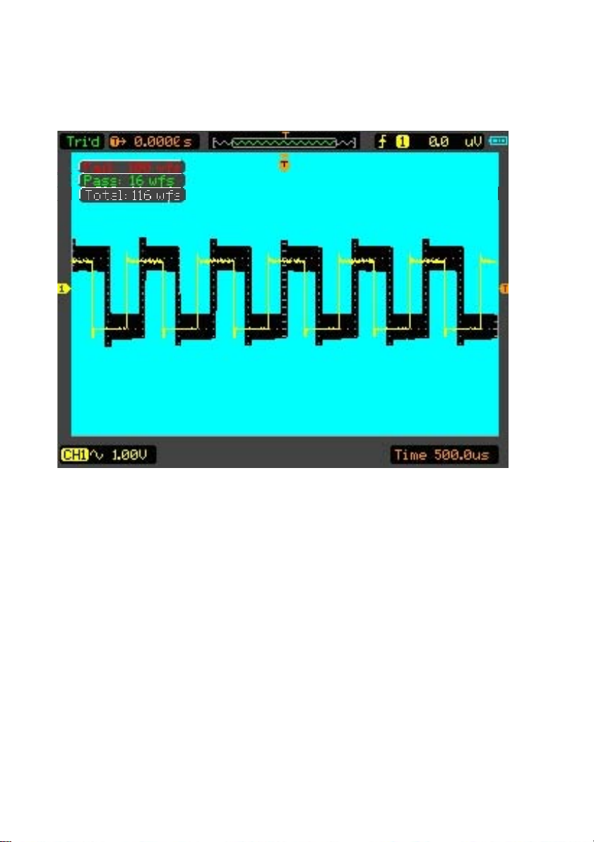
Pass/Fail test – Mask (Blue) and signal (yellow) display
54 MS6000-EU-EN-V1.3 7/12
Page 55

4.5.5 DISPLAY
The waveform display is affected by settings of the oscilloscope. A waveform can be measured once it is
captured. The different styles to display a waveform on the screen give significant information about it.
There are two modes to display waveforms; Single-window and Double window.
Refer to Horizontal Controls
Press the Utility button and then the DISPLAY button on page 4 of the Utility menu.
Options Settings Comments
Type (F1)
Persistency (F2)
DSO mode (F3)
Contrast (F4) 0-15 Use the Multifunction control to set the display contrast.
Grid (F2)
Grid Intensity (F3)
Refresh Rate (F4)
Wave Bright (F2)
BL Keep (F3)
Menu Keep (F4)
for more information.
Vectors
Dots
Auto
0.2S-8S selectable
Infinite
YT
XY
Dotted Line
Real Line
Off
Auto
30, 40, 50 Frames
Unlimited
5, 10, 30, 60 Sec
Unlimited
5, 10, 30, 60 Sec
‘Vectors’ fills up the space between adjacent sample point s
in the display; ‘Dots’ displays the sample points only.
Length of time to display each displayed sample point.
YT – normal or standard signal view
XY – XY format
Menu page 2
Set up for display of the grid lines.
Use the Multifunction control to set the brightness of the
displays Grid lines.
Set refresh rate of display (default is Auto)
Menu Page 3
Use multifunction control arrow keys to change waveform
brightness.
Set how long the Backlight is on before it turns off
Set how long the Menu is displayed before it turns off
55 MS6000-EU-EN-V1.3 7/12
Page 56
4.5.6 ACQUIRE
The acquisition modes of an oscilloscope control how waveform points are generated from
sample points.
Options Settings Comments
Type (F1)
Mode (F2)
(Real Time)
Averages (F3)
(Real Time)
LongMem (F4) 4K, 40K, 512K Memory depth - Select the memory depth.
Back (F5) Go back to the main Utility menu
Normal: (Sample mode) creates a waveform in the oscilloscope by saving a collection of sample points.
The samples are taken at each waveform interval.
Press the Utility button and then the ACQUIRE key on page 4 of the Utility menu.
Real Time
Equ-Time
Normal
Peak
Average
4
16
64
128
Acquire waveforms by real-time digital technique.
Rebuild waveforms by equivalent sample technique.
Normal: Acquire and accurately display most waveforms.
Peak: Detect glitches and eliminate the possibility of aliasing.
Average: Reduce random or uncorrelated noise in signal
display. The number of averages is selectable.
Mode (F2) must be set top Average.
Select the number of averages.
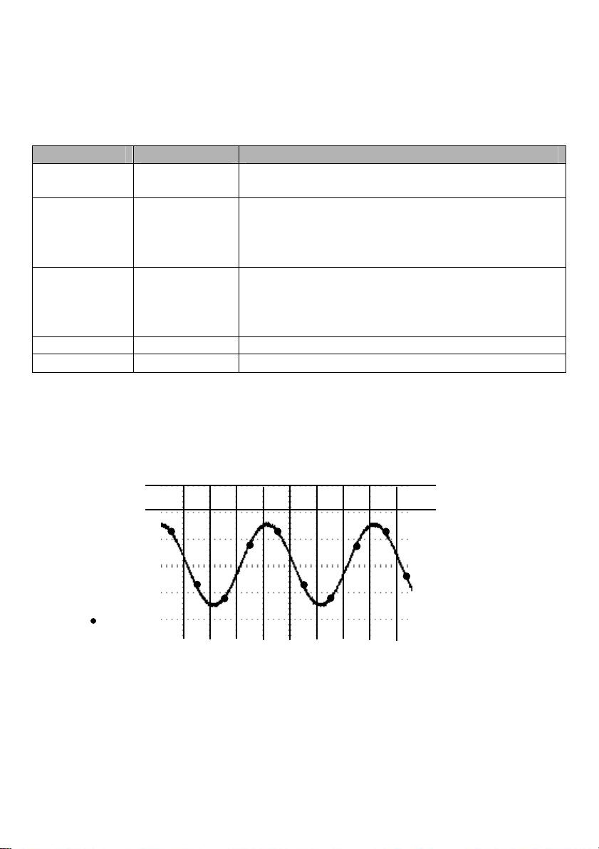
Normal Acquisition Intervals
837 24561 9 10
Sample Points
Normal Mode Acquires a Single Sample Point in each Waveform Interval
56 MS6000-EU-EN-V1.3 7/12
Page 57
Peak Detect: Use this mode to detect glitches within 10ns and to limit the possibility of aliasing. This
mode is valid at the TIME/DIV setting of 4µs/div or slower. Once the TIME/DIV setting is adjusted to
4µs/div or faster, the acquisition mode will change to Normal because the sample rate is fast enough
and Peak Detect is unnecessary. The oscilloscope does not display a message that the mode has been
changed to Normal.
Average: Use this mode to reduce random or uncorrelated noise in the signal to be displayed. Acquire
data in Normal mode and then average some number of waveforms. Choose the number of acquisitions
(4, 16, 64 or 128) to average for the waveform.
Stopping the Acquisition: When running acquisition mode, the waveform display is LIVE. Stop the
acquisition (press the RUN/STOP button) to freeze the display. In either mode, the waveform display
can be scaled or positioned by vertical and horizontal controls.
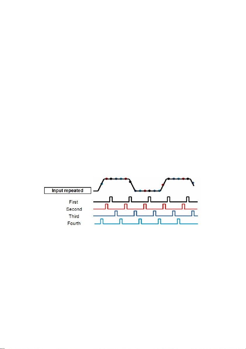
Equivalent Acquisition: Repeats the Normal acquisition. Use this mode to take a specific observation
on repeatedly displayed periodic signals. A resolution of 40ps can be obt ained, (i.e. 25GS/s sample rate),
which is much higher than that obtained in real-time acquisition mode.
The acquisition principle is as follows.
As shown above, aquire a repeatable input signal. Sample the signal at various intervals. Store the
digital values in memory. The Sample points can now be use to recreate the waveform.
57 MS6000-EU-EN-V1.3 7/12
Page 58

4.5.7 Fast Action Buttons
AUTO: Automatically set the oscilloscope controls to generate a usable display of the input signals.
Refer to the following table for relative content.
RUN/STOP: Continuously acquire waveforms or stop the acquisition.
4.5.8 AUTOSET
Autoset is one of the most useful modes of the digital oscilloscope. When the AUTO button is pressed,
the oscilloscope will identify the type of waveform (sine or square) and adjust controls according to the
input signal so that it can accurately display the waveform.
Functions Settings made automatically
Acquire Mode Adjusts to Normal or Peak Detect
Cursor Off
Display Format Sets to YT
Display Type Sets to Vectors for an FFT spectrum; otherwise, unchanged
Horizontal Position Adjusted
TIME/DIV Adjusted
Trigger Coupling Adjusts to DC, Noise Reject, LF Reject or HF Reject
Trigger Holdoff Minimum
Trigger Level Sets to 50%
Trigger Mode Auto
Trigger Source Adjusted
Trigger Slope Adjusted
Trigger T ype Edge
Trigger Video Sync Adjusted
Trigger Video Standard Adjusted
Vertical Bandwidth Full
Vertical Coupling
Volts Adjusted
DC (if GND was chosen before); AC for the video signal; otherwise,
unchanged
58 MS6000-EU-EN-V1.3 7/12
Page 59

The Autoset function examines all channels for signals and displays corresponding waveforms. Autoset
determines the trigger source according to the following conditions.
If multiple channels receive signals, the oscilloscope will use the channel with the lowest
frequency signal as the trigger source.
If no signals are found, the oscilloscope will use the lowest-numbered channel displayed in
Autoset as the trigger source.
If no signals are found and no channels are displayed, the oscilloscope will display and use
Channel 1 as the trigger source.
Sine Wave:
When the Autoset function is used and the oscilloscope determines that the signal is similar to a sine
wave, the oscilloscope displays the following options:
Sine Wave Options Details
Multi-cycle Sine Display multiple cycles that have appropriate vertical and horizontal scales.
Single-cycle Sine Set the horizontal scale to display approx. one cycle of waveform.
Convert the input time-domain signal to its frequency components and
FFT
Cancel Setup Allow the oscilloscope to recall the previous setup.
Square Wave or Pulse:
When the Autoset function is used and the oscilloscope determines that the signal is similar to a square
wave or pulse, the oscilloscope displays the following options:
Square Wave Options Details
Multi-cycle Square Display multiple cycles that have appropriate vertical and horizontal scales.
Single-cycle Square
Rising Edge Display the rising edge.
Falling Edge Display the falling edge.
Cancel Setup Allow the oscilloscope to recall the previous setup.
display the result as a graph of frequency versus amplitude (spectrum). See
Section 5.3.1 Math FFT for more information.
Set the horizontal scale to display approx. one cycle of waveform. The
oscilloscope displays Min., Mean and Positive Width automatic
measurements.
59 MS6000-EU-EN-V1.3 7/12
Page 60

Chapter 5 - Multimeter Operation
Multimeter Operation Window
Figure 7-1 Multimeter operation window
Description
1) Measurement mode indicators:
DC: Direct current measurement
AC: Alternating current measurement
2) Input jacks and connection diagrams.
3) Manual/Auto range indicators, among which the MANUAL refers to measuring ra nge in
manual operation mode and Auto means the measuring range in automatic operation
mode.
4) Measured value display.
5) Bar graph indicator.
6) DC or AC Measurement mode control.
7) Absolute/Relative magnitude measuring control: The sign “||” expresses the absolute
magnitude measuring control and “
control.
8) Manually or automatically measuring range control.
∆” represents the relative magnitude measuring
60 MS6000-EU-EN-V1.3 7/12
Page 61

Operating the Multimeter
From the the oscilloscope window, press the OSC/DMM key, the oscilloscope will switch to
the multimeter mode window. The screen will then display the measurement mode window
that was in use the last time the multimeter was switched OFF. When switching to the
multimeter measurement mode for the first time, the default measurement mode is DC
voltage.
Measuring Resistance Values
To measure a resistance, perform the following:
1) Press the R key; the resistance measurement window appears on the screen.
2) Insert the black lead into the COM banana jack input and the red lead into the V/ Ω/C
banana jack input.
3) Connect the red and black test leads to the resistor. The resistance value is shown on the
screen in Ohms. Refer to the screen image in figure 7-2.
Figure 7-2 Resistance Measurement
61 MS6000-EU-EN-V1.3 7/12
Page 62

Making a Diode Measurement
To make a measurement on the diode, perform the following:
1) Press the diode key; the diode symbol appears at the top of the screen. .
2) Insert the black lead into the COM banana jack input and the red lead into the V/ Ω/C
banana jack input.
3) Connect the red and black leads to the diode; the voltage value of the diode is displaye d
on the screen in volts. The screen will then resemble the image in figure 7-3.
Figure 7-3 Diode Measurement
62 MS6000-EU-EN-V1.3 7/12
Page 63

Making a Continuity Measurement
To perform a Continuity test, perform the following:
)
1) Press the
)
) key; the
2) Insert the black lead into the COM banana jack input and the red lead into the V/ Ω/C
banana jack input.
3) Connect the red and black leads to the test points. If the resistance value of the tested
points is less than 30 Ω, a beep will sound from the test tool. The screen will resemble the
image in figure 7-4.
)
)
) indictor appears at the top of the screen.
Figure 7-4 Continuity Measurement
63 MS6000-EU-EN-V1.3 7/12
Page 64
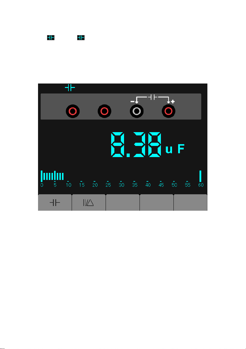
Making a Capacitance Measurement
To measure a capacitance, do the following:
1) Press the key; the symbol appears at the top of the screen.
2) Insert the black lead into the COM banana jack input and the red lead into the V/ Ω/C
banana jack input.
3) Connect the red and black leads to the capacitor; the capacitance v alue is displayed on
the screen in µF or nF. The screen will resemble the image in figure 7-5.
Figure 7-5 Capacitance Measurement
64 MS6000-EU-EN-V1.3 7/12
Page 65
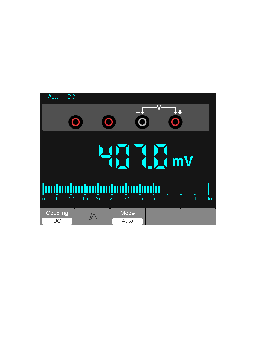
Making a DC Voltage Measurement
To measure a DC voltage, perform the following:
1) Press the V key; the Auto DC icon appears at the top of the screen.
2) Insert the black lead into the COM banana jack input and the red lead into the V/ Ω/C
banana jack input.
3) Connect the red and black leads to the measurement points; the voltage value of the
measured points is displayed on the screen. The screen will resemble the image in figure
7-6.
Figure 7-6 DC voltage Measurement
65 MS6000-EU-EN-V1.3 7/12
Page 66
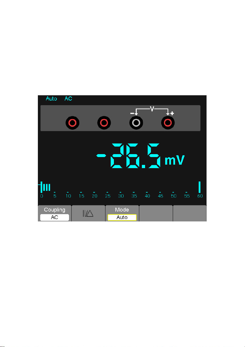
Making an AC Voltage Measurement
To measure the AC voltage, perform the following:
1) Press the V key; the DC icon appears on the screen.
2) Press the F1 key; the AC icon appears on the screen.
3) Insert the black lead into the COM banana jack input and the red lead into the V/ Ω/C
banana jack input.
4) Connect the red and black leads to the measured points; the AC voltage value of the
measured points will be displayed on the screen. T he screen will resemble the image in
figure 7-7.
Figure 7-7 AC voltage Measurement
66 MS6000-EU-EN-V1.3 7/12
Page 67
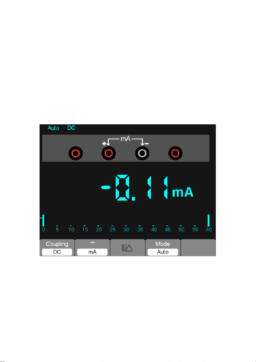
Making a DC Current Measurement
To measure a DC current smaller than 600 mA, perform the following :
1) Press the A key; the DC icon appears on the screen. The unit of measure on the main
reading screen is mA. Press F2 to switch the measurement between mA and 10A.
600mA is acquiescence.
2) Insert the black lead into the COM banana jack input and the red lead into the mA banana
jack input.
3) Connect the red and black leads to the measured points; the DC current value of
measured
points will be displayed on the screen. The screen will resemble the imag e in figure 7-8.
NOTE: For current measurements 5 amps and above, limit the measurement time to 15
seconds and allow for a 1 minuite cool down between measurements.
Figure 7-8 DC current Measurement for 600 mA
67 MS6000-EU-EN-V1.3 7/12
Page 68
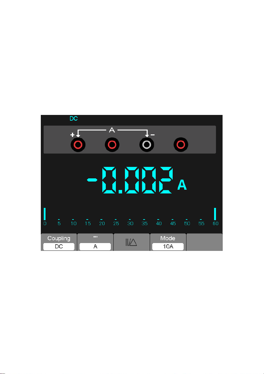
To measure a DC current greater than 600 mA, perform the following:
1) Press the A key; the DC icon appears on the screen. The unit of measure on the main
reading screen is mA.
2) Press the F2 key to switch to 10A measurement, the unit of measure on the main reading
is A.
3) Insert the black lead into the COM banana jack input and the red lead into the 10A banana
jack input.
4) Connect the red and black leads to the measured points; the DC current value of the
measured points will be displayed on the screen.
5) Press F2 to return to 600 mA measurement.
The screen will resemble the image in figure 7-9.
Figure 7-9 DC Current Measurement for 10A
68 MS6000-EU-EN-V1.3 7/12
Page 69
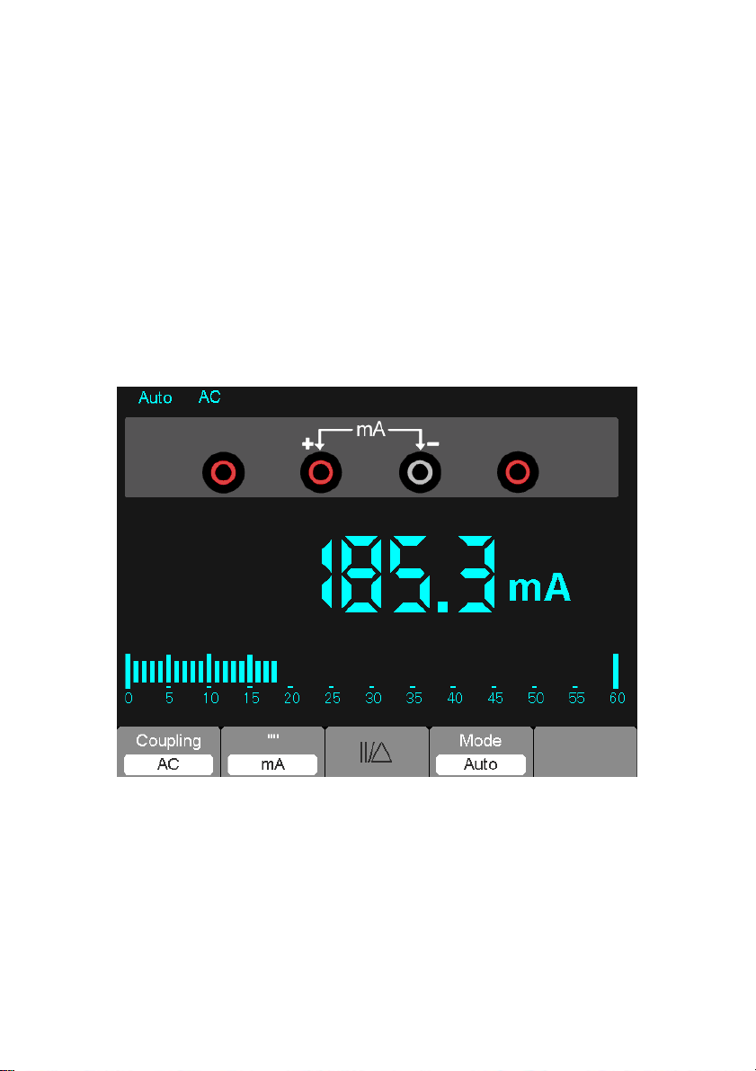
Making an AC Current Measurement
To measure an AC current smaller than 600 mA, perform the follow ing:
1) Press the A key; the DC icon appears on the screen. The unit of measure on the main
reading screen is mA; the mA icon will display on the bottom of the screen, press F2 to
switch the measurement between mA and 10A. 600mA is acquiescence.
2) Press the F1 key once; the AC icon will display on the screen.
3) Insert the black lead into the COM banana jack input and the red lead into the mA banana
jack input.
4) Connect the red and black leads to the measured points; the AC current value of
measured points will be displayed on the screen. The screen will resemble the image
shown in figure 7-10.
NOTE: For current measurements 5 amps and above, limit the measurement time to 15
seconds and allow for a 1 minuite cool down between measurements.
Figure 7-10 AC Current Measurement for 600 mA
69 MS6000-EU-EN-V1.3 7/12
Page 70

To measure an AC current greater than 600 mA, perform the following:
1) Press the A key; the DC icon appears on the screen. The unit on the main reading screen
is mA.
2) Press F2 key to switch to the 10A measurement mode, the unit on the main reading
screen is A.
3) Press the F1 key once and the AC icon will display on the the screen.
4) Insert the black lead into the COM banana jack input and the red lead into the 10A banana
jack input.
5) Connect the red and black leads to the measured points and the AC current value of the
measured points will be displayed on the screen.
6) Press F2 to return to the 600 mA measurement mode.
The screen will resemble the image shown in figure 7-11.
Figure 7-11 AC Current Measurement for 10A
70 MS6000-EU-EN-V1.3 7/12
Page 71
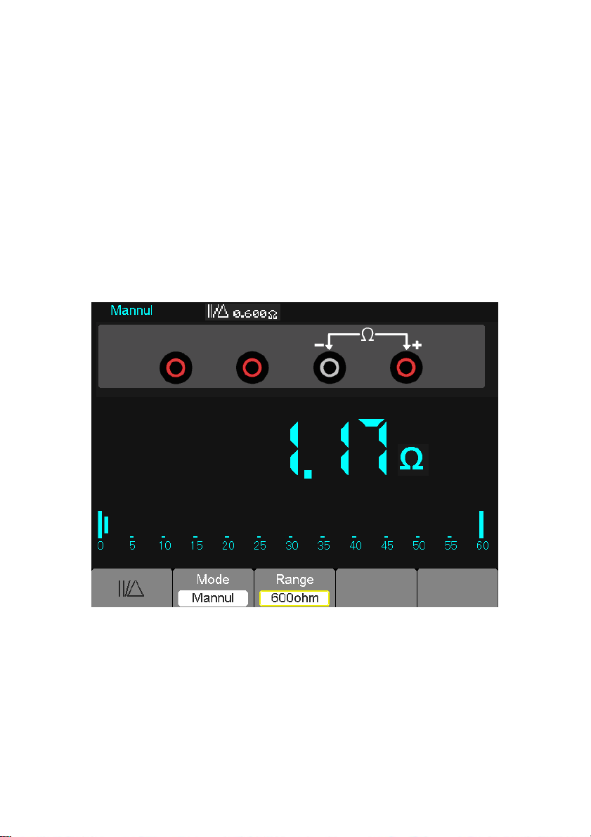
Taking a Relative Measurement
A relative measurement is a measurement taken and compared to a stored reference value.
The resultant display represents the measurement minus the reference value.
The following example illustrates the relative measurement process. The first step is
to store a reference value.
1) Press the ‘Ω’ key.
2) Insert the black lead into the COM banana jack input and the red lead into the V/ Ω/C
banana jack input.
3) Connect the red and black test leads to a resistor. The resistance value is sho wn on the
screen in Ohms.
4) When the reading stabilizes, press the F1 key; the ||/is displayed on the top of the
screen.
The saved reference value is displayed.
The screen will resemble the image shown in figure 7-12.
Figure 7-12 Relative Measurement
71 MS6000-EU-EN-V1.3 7/12
Page 72
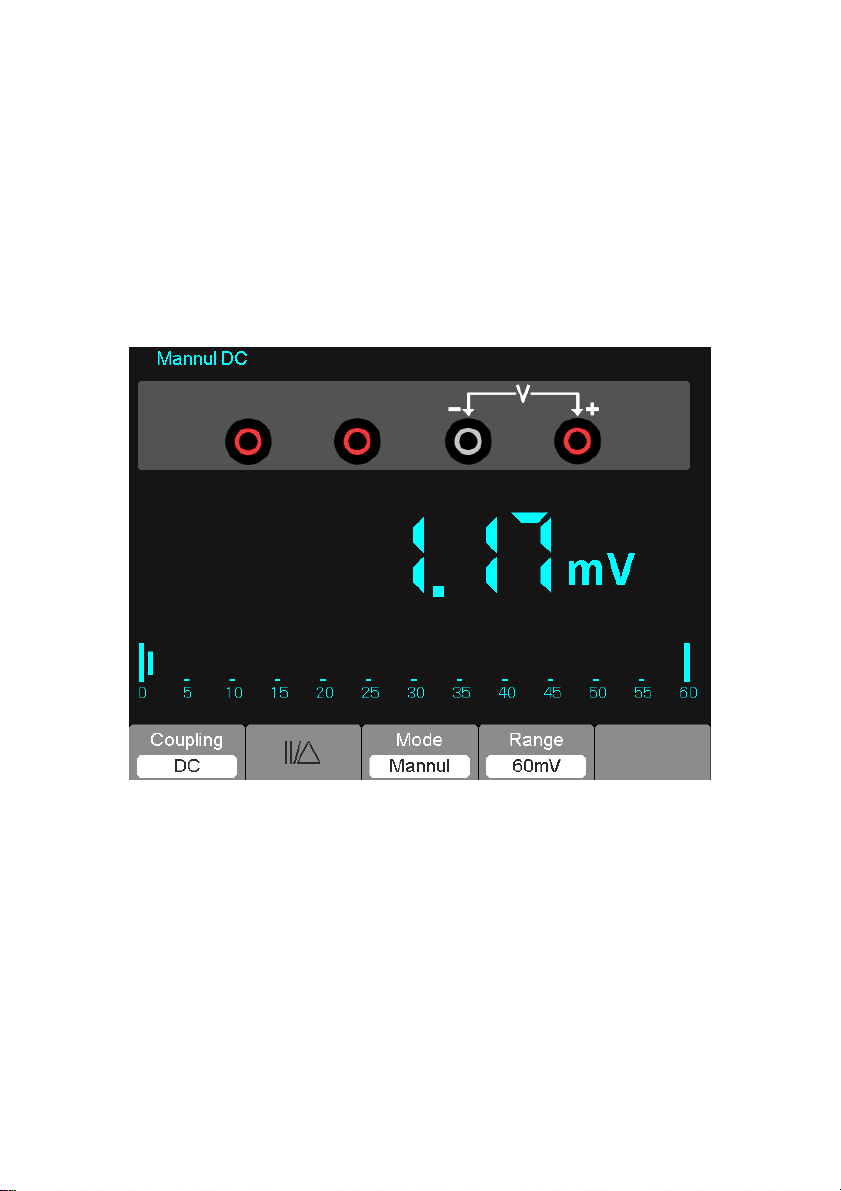
Selecting Automatic/Manual Range Adjustment
The default mode is the automatic range mode. For example: In the DC voltage mode,
to switch to the manual range, perform the following steps:
1) Press F3 to enter the manual range mode; the Manual icon is displayed.
2) In the manual range mode, the measuring range is increased each time the F4 is pressed.
When the highest range is reached, the next F4 key press moves the m et er to the lowest
range.
3) Press F3 to revert to the automatic range mode; the Auto icon is displayed again.
Attention: Capacitance measurements cannot be made in the manual range mode.
The screen will resemble the image shown in figure 7-13.
Figure 7-13 Manual Range Mode
72 MS6000-EU-EN-V1.3 7/12
Page 73

Chapter 6 - Troubleshooting
6.1 Problem Solving
1. If the oscilloscope will not power ON, follow these steps:
1 Check the power cord to verify it has been connected properly;
2 Check the power on/off button to ensure it has been pushed;
3 Restart the oscilloscope.
Contact your local Extech distributor or the Extech Technical Support department if the problem persists.
2. If waveforms will not display when the oscilloscope is switched ON:
1 Check the probe to assure it is properly connected to the input BNC;
2 Check the channel switch (such as CH1, CH2 menu button s) to make sur e it has been
turned on;
3 Check the input signal to verify it has been connected to the probe correct ly;
4 Verify that all measured circuits indeed have signals to output;
5 Raise the magnitude for DC signals;
6 Press the Auto button to perform an automatic detection of signals.
Contact Extech Technical Support department if there is still no display of waveforms.
3. If the waveform of the input signal is seriously distorted, follow these steps:
1 Check the probe to assure a proper connection to the channel BNC;
2 Check the probe to assure a good connection to the measured object;
3 Check the probe to verify that it has been well calibrated. Otherwise, refer to the content
regarding Calibration in this manual.
4. If the waveform is moving continuously on the screen and can not be triggered:
1 Check the trigger source to ensure that it is consistent with the input channel;
2 Check the trigger level to assure a correct setting.
3 Check the trigger mode to confirm that it is an appropriate selection for the input signal.
The default trigger mode is Edge trigger. However, edge triggering it is not suitable for
every type of input signal.
5. If the meter will not display current measurements:
The internal fuses may have opened. The meter is protected by two fast acting fuses not
accessible to the user. The fuses are rated: 1A (600V) and 12A (600V) fast acting.
Please contact a local Extech distributor or the Extech Technical Support department for
assistance in locating a local service center.
Page 74

Chapter 7 - Specifications
7.1 Technical Specifications
All published specifications apply to the MS6000 series oscilloscopes. Before checkin g an
oscilloscope to verify its compliance with these specifications, ensure that the oscilloscope
meets the following conditions:
The oscilloscope must have undergone a twenty minute warm-up period under the
specified operating temperature.
The ‘Do Self Cal’ operation must be performed through the Utility menu if the operating
temperature changes by more than 5
The oscilloscope must be within the factory calibration interval.
All specifications are guaranteed unless noted ‘typical’.
Oscilloscope Specifications
Horizontal
Sample Rate Range 1GS/s
Waveform Interpolation (sin x)/x
Record Length
TIME/DIV Range
Sample Rate and
Delay Time Accuracy
Maximum 1M samples per single-channel; maximum 512K
samples per dual-channel
MS6060
MS6100
4ns/div to 40s/div, in a 2, 4, 8
sequence
±50ppm over any ≥1ms time interval
o
C.
MS6200
2ns/div to 40s/div, in a 2, 4, 8
sequence
74 MS6000-EU-EN-V1.3 7/12
Page 75

Delta Time Measurement
Accuracy
(Full Bandwidth)
Position Range
Vertical
A/D Converter
Single-shot, Normal mode
± (1 sample interval +100ppm × reading + 0.6ns)
>16 averages
± (1 sample interval + 100ppm × reading + 0.4ns)
Sample interval = s/div ÷ 200
MS6060
MS6100
4ns/div to 8ns/div (-8div × s/div) to 20ms
20ns/div to 80μs/div (-8div × s/div) to 40ms
200μs/div to 40s/div (-8div × s/div) to 400s
MS6200
2ns/div to 10ns/div (-4div × s/div) to 20ms
8-bit resolution,
each channel is sampled simultaneously
VOLTS Range 2mV/div to 5V/div at input BNC
Position Range
Analog Bandwidth in
Normal and Average
modes at BNC or with probe, DC
Coupled
Selectable Analog Bandwidth Limit,
typical
Low Frequency Response (-3db) ≤10Hz at BNC
Rise Time at BNC, typical
2mV/div to 200mV/div, ±2V
>200mV/div to 5V/div, ±50V
2mV/div to 20mV/div, ±400mV
50mV/div to 200mV/div, ±2V
500mV/div to 2V/div, ±40V
5V/div, ±50V
20MHz
MS6060 MS6100 MS6200
<5.8ns 3.5ns <1.8ns
75 MS6000-EU-EN-V1.3 7/12
Page 76

±3% for Normal or Average acquisition mode, 5V/div
DC Gain Accuracy
DC Measurement Accuracy,
Average Acquisition Mode
Volts Measurement Repeatability,
Average Acquisition Mode
Note: Bandwidth reduced to 6MHz when using a 1X probe.
to 10mV/div
±4% for Normal or Average acquisition mode,
5mV/div to 2mV/div
Measurement Type: Average of ≥16 waveform s wit h
vertical position at zero
Accuracy: ± (3% × reading + 0.1div + 1mV) when
10mV/div or greater is selected
Measurement Type: Average of ≥16 waveform s wit h
vertical position not at zero
Accuracy: ± [3% × (reading + vertical position) + 1%
of vertical position + 0.2div]
Add 2mV for settings from 2mV/div to 200mV/div;
add 50mV for settings from 200mV/div to 5V/div
Delta volts between any two averages of ≥16
waveforms acquired under same setup and ambient
conditions
76 MS6000-EU-EN-V1.3 7/12
Page 77

Trigger
Trigger Sensitivity
(Edge Trigger Type)
Coupling Sensitivity
MS6060
MS6100
1div from DC to
10MHz;
1.5div from 10MHz
to Full
DC
Source
CH1
CH2
AC Attenuates signals below 10Hz
HF Reject Attenuates signals above 80kHz
MS6200
1.5div from 10MHz
to 100MHz;
2div from 100MHz
to Full
Same as the DC-coupled limits for frequencies above
150kHz; attenuates signals below 150kHz
Trigger Level Range
LF Reject
Source Range
CH1, CH2 ±8 divisions from center of screen
Source Accuracy Trigger Level
Accuracy, typical
(Accuracy is for
signals having rise
CH1CH2
0.2div × volts/div within ±4 divisions from center of
screen
and fall times ≥20ns)
Set Level to 50%,
typical
Operates with input signals ≥50Hz
Note: Bandwidth reduced to 6MHz when using a 1X probe.
77 MS6000-EU-EN-V1.3 7/12
Page 78

Video Trigger Type
CH1, CH2
Signal Formats and
Field Rates, Video
Trigger Ty pe
Holdoff Range 100ns to 10s
Pulse Width
Trigger
Pulse Width Trigger
Mode
Pulse Width Trigger
Point
Pulse Width Range Selectable from 20ns to 10s
Source Range
Supports NTSC, PAL and
SECAM broadcast systems for
any field or any line
Trigger when < (Less than), > (Greater than), = (Equal), or ≠ (Not
Equal); Positive pulse or Negative pulse
Equal: The oscilloscope triggers when the trailing edge of the puls e
crosses the trigger level.
Not Equal: If the pulse is narrower than the specified width, the trigger
point is the trailing edge. Otherwise, the oscilloscope triggers when a
pulse continues longer than the time specified as the Pulse Width.
Less than: The trigger point is the trailing edge.
Greater than (also called overtime trigger): The oscilloscope triggers
when a pulse continues longer than the time specified as the Puls e
Width.
Peak-to-peak amplitude of 2
divisions
78 MS6000-EU-EN-V1.3 7/12
Page 79

Slope Trigger
Slope Trigger Mode
Slope Trigger Point
Time Range Selectable from 20ns to 10s
Overtime Trigger The leading edge: Rising edge or Falling edge; Time Setting: 20-10s
Alter (Swap)
Trigger
CH1 Internal Trigger: Edge, Pulse Width, Video, Slope
CH2 Internal Trigger: Edge, Pulse Width, Video, Slope
Trigger when < (Less than), > (Greater than), = (Equal), or ≠ (Not
Equal); Positive slope or Negative slope
Equal: The oscilloscope triggers when the waveform slope is equal to
the set slope.
Not Equal: The oscilloscope triggers when the waveform slope is not
equal to the set slope.
Less than: The oscilloscope triggers when the waveform slope is less
than the set slope.
Greater than: The oscilloscope triggers when the waveform slope is
greater than the set slope.
79 MS6000-EU-EN-V1.3 7/12
Page 80

Acquisition
Acquisition Modes Normal, Peak Detect, and Average
Acquisition Rate,
typical
Up to 2000 waveforms per second per channel (Normal acquisition
mode, no measurement)
Single Sequence Acquisition Mode Acquisition Stop Time
Normal, Peak Detect
Upon single acquisition on all
channels simultaneously
After N acquisitions on all
Average
channels simultaneously, N can
be set to 4, 8, 16, 32, 64 or 128
Inputs
Input Coupling DC, AC or GND
Input Impedance,
DC coupled
1MΩ ±2% in parallel with 20pF ±3pF
Probe Attenuation 1X, 10X
Supported Probe
Attenuation
Maximum Input
Voltage
1X, 10X, 100X, 1000X
Overvoltage Category Maximum Voltage
CAT I and CAT II
300V
Category
CAT III 150V
(10×), Installation
RMS
(1×)
RMS
Installation Category II: derate at 20dB/decade above 100kHz to 13V
peak AC at 3MHz* and above. For non-sinusoidal waveforms, peak
value must be less than 450V. Excursion above 300V should be of less
than 100ms duration. RMS signal level including all DC components
removed through AC coupling must be limited to 300V. If these values
are exceeded, damage to the oscilloscope may occur.
80 MS6000-EU-EN-V1.3 7/12
Page 81

Measurements
Voltage difference between cursors: V
Cursors
Time difference between cursors: T
Reciprocal of T in Hertz (1/ΔT)
Frequency, Period, Mean, Peak-to-peak, CycleRMS, Minimum,
Automatic
Measurements
Maximum, Rise Time, Fall Time, Positive Width, Negative Width,
Delay 1-2↑, Delay 1-2↓, +Duty, -Duty, Base, Top, Middle, Amplitude,
Overshoot, Preshoot, RMS, Off
General Specifications
Display
Display Type 5.6 Inch width LED Backlight Display
Display Resolution 240 (Vertical) X 320 (Horizontal) pixels
Display Contrast Adjustable (16 steps) with a progress bar
Probe Compensator Output
Output Voltage,
typical
About 2Vpp into ≥1MΩ load
Frequency, typical 1kHz
Internal Memory
2G SD Card
Accommodates up to 32G card (accessible through battery
compartment)
Power Supply
Supply Voltage
100-120VAC
120-240VAC
Power Consumption <30W, (approx. 3 hours)
Fuses Two (2) fast-acting internal fuses: 1A (600V) and 12A (600V)
Battery 7.4V li-ion rechargeable
(±10%), 45Hz to 440Hz
RMS
(±10%), 45Hz to 66Hz
RMS
81 MS6000-EU-EN-V1.3 7/12
Page 82

82 MS6000-EU-EN-V1.3 7/12
Page 83

Environmental
Operating: 32Ԭ to 122Ԭ (0Ԩ to 50Ԩ)
Temperature
Nonoperating: -40Ԭ to 159.8Ԭ (-40Ԩ to +71Ԩ)
Cooling Method Convection
+104Ԭ or below (+40Ԩ or below): ≤90% relative humidity
Humidity
106Ԭ to 122Ԭ (+41Ԩ to 50Ԩ): ≤60% relative humidity
Altitude Operating and Non-operating 3,000m (10,000 feet)
Random Vibration
Non-operating
0.31g
10 minutes on each axis
2.46g
minutes on each axis
from 50Hz to 500Hz,
RMS
from 5Hz to 500Hz, 10
RMS
Mechanical Shock Operating 50g, 11ms, half sine
Mechanical
Length 245mm (10”)
Size
Weight
Height 163mm (6.4”)
Depth 52mm (2”)
Excludes packing and
accessories
83 MS6000-EU-EN-V1.3 7/12
1.2 Kg (2.6 lbs.)
Page 84

84 MS6000-EU-EN-V1.3 7/12
Page 85

Meter Mode
Maximum Resolution 6000 Counts
DMM Testing Modes Voltage, Current, Resistance, Capacitance, Diode &
Continuity
Maximum Input Voltage AC : 600V DC : 800V
Maximum Input Current AC : 10A DC : 10A
Input Impedance 10MΩ
Meter Specification
Range Accuracy (of rdg.) Resolution
DC Voltage
AC Voltage
DC Current
AC Current
60.00mV(manual) 10uV
600.0mV 100uV
6.000V 1mV
60.00V 10mV
600.0V 100mV
800V
60.00mV(manual) 10uV
600.0mV(manual) 100uV
6.000V 1mV
60.00V 10mV
600.0V
60.00mA ±1.5%±1digit 10uA
600.0mA ±1%±1digit 100uA
6.000A 1mA
10.00A
60.00mA ±1.5%±3digits 10uA
600.0mA ±1%±1digit 100uA
6.000A 1mA
10.00A
±1%±1digit
1V
±1%±3digits
100mV
±1.5%±3digits
10mA
±1.5%±3digits
10mA
85 MS6000-EU-EN-V1.3 7/12
Page 86

Resistance
600.0 0.1Ω
6.000K 1Ω
60.00K 10Ω
600.0K 100Ω
6.000M
60.00M ±1.5%±3digits 10KΩ
Capacitance
40.00nF 10pF
400.0nF 100pF
4.000uF 1nF
40.00uF 10nF
400.0uF
Note: The smallest capacitance value that can be measured is 5nF
Diode
0V~2.0V
On-off Test < 30Ω
±1%±1digit
1KΩ
±1.75%±10digits
100nF
86 MS6000-EU-EN-V1.3 7/12
Page 87

Chapter 8 - General Care and Cleaning
8.1 General Care
Do not expose the LCD display to direct sunlight for long periods of time.
To avoid damage to the oscilloscope or probes, do not expose them to sprays, liquids, or
solvents.
8.2 Cleaning
Examine the oscilloscope and probes as often as operating conditions require. To clean the
exterior surface, perform the following steps:
1 Use a lint-free cloth to remove floating dust on the outside of the oscilloscope and
probes. Take care to avoid scratching the display.
2 Use a soft cloth dampened with water to clean the oscilloscope. For more efficient
cleaning, you may use an aqueous solution of 75% isopropyl alcohol.
Note: To avoid damage to the surface of the oscilloscope or probes, do not use
corrosive or chemical cleaning agents.
Copyright © 2012 Extech Instruments Corporation (a FLIR company)
All rights reserved including the right of reproduction in whole or in part in any form
ISO-9001 Certified
87 MS6000-EU-EN-V1.3 7/12
 Loading...