EXFO PSO-200 User Manual

PSO-200

Optical Modulation Analyzer

User Guide

Copyright © 2010–2013 EXFO Inc. All rights reserved. No part of this publication may be reproduced, stored in a retrieval system or transmitted in any form, be it electronically, mechanically, or by any other means such as photocopying, recording or otherwise, without the prior written permission of EXFO Inc. (EXFO).

Information provided by EXFO is believed to be accurate and reliable. However, no responsibility is assumed by EXFO for its use nor for any infringements of patents or other rights of third parties that may result from its use. No license is granted by implication or otherwise under any patent rights of EXFO.

EXFO’s Commerce And Government Entities (CAGE) code under the North Atlantic Treaty Organization (NATO) is 0L8C3.

The information contained in this publication is subject to change without notice.

Trademarks

EXFO’s trademarks have been identified as such. However, the presence or absence of such identification does not affect the legal status of any trademark.

Units of Measurement

Units of measurement in this publication conform to SI standards and practices.

Patents

EXFO’s Universal Interface is protected by US patent 6,612,750.

Version number: 2.0.1

ii PSO-200

Contents

Certification Information ....................................................................................................... vi

European Community Declaration of Conformity ................................................................. vii

1 Introducing the PSO-200 Optical Modulation Analyzer ............................. 1

Main Features .........................................................................................................................1

Conventions ............................................................................................................................3

2 Safety Information ....................................................................................... 5

Laser Safety Information .........................................................................................................5

Electrical Safety Information ...................................................................................................6

3 Getting Started with Your Optical Modulation Analyzer ........................... 9

Installing the EXFO Universal Interface (EUI) ...........................................................................9

Cleaning and Connecting Optical Fibers ...............................................................................10

Starting and Exiting the Optical Modulation Analyzer Application .......................................12

4 Setting Up the Optical Modulation Analyzer ........................................... 13

Configuring the Input Signal ................................................................................................13

Setting Other Acquisition Parameters ...................................................................................16

Setting File Autonaming .......................................................................................................18

Identifying Acquisitions ........................................................................................................20

Setting Analysis Parameters ..................................................................................................22

Using Special Modulation Modes .........................................................................................24

Using an External Local Oscillator .........................................................................................27

Locking the Remote Unit ......................................................................................................31

5 Performing Acquisitions ............................................................................ 33

Starting and Stopping an Acquisition ...................................................................................33

Clearing Data During an Acquisition .....................................................................................34

Saving Acquisitions to a File .................................................................................................35

Activating Trigger-Based Acquisitions ...................................................................................36

6 Customizing the Graph and Data Layout ................................................. 39

Selecting and Customizing the Layout ..................................................................................39

Constellation Chart ...............................................................................................................41

Eye Diagrams ........................................................................................................................43

Pattern Diagrams ..................................................................................................................47

Y-Axis Auto Scaling (All Graphs) ............................................................................................47

Optical Modulation Analyzer iii

Contents

7 Viewing and Analyzing Results ..................................................................49

Opening an Existing Acquisition File .....................................................................................49

Viewing Acquisition Information ..........................................................................................50

Playing Back Acquisition Files ...............................................................................................51

Zooming and Moving Graphs ...............................................................................................52

Displaying and Setting X-Axis Values ....................................................................................53

Displaying Graphs in Color Grade Mode ...............................................................................54

Displaying Multiple Bursts Simultaneously (Persistence) .......................................................55

Setting Number of Symbol Periods for Eye Diagrams ...........................................................55

Using the Measurement Tables .............................................................................................56

Using Graph Markers ............................................................................................................58

Viewing Signal Distribution Using Histograms ......................................................................60

Distinguishing Data Points from Transitions .........................................................................62

Using Pattern Masks .............................................................................................................64

Using Averaging to Improve Results .....................................................................................70

Applying Advanced Signal Processing Algorithms ................................................................72

Applying Data Filtering .........................................................................................................76

8 Bit Pattern Analysis and the Gearbox ........................................................79

Basic Gearbox Setup Details ..................................................................................................80

Exporting Symbol Patterns ....................................................................................................83

Importing User-Defined Symbol Patterns ..............................................................................84

Performing Detailed Bit Pattern Analysis with the Gearbox ...................................................87

Using PRBS or User-Defined Bit Patterns with the Gearbox .................................................100

Exporting Gearbox Setups ..................................................................................................104

Obtaining and Using Bit/Symbol Error Rates .......................................................................105

9 Post-Processing and Reanalyzing Data ....................................................109

Installing and Using the Application on a Computer ..........................................................109

Installing and Activating Software Options ........................................................................111

Exporting Data ....................................................................................................................113

Copying Graph and Measurements to Clipboard ................................................................114

Reanalyzing Acquisitions with New Settings .......................................................................115

Reverting to Original File ....................................................................................................116

10 Maintenance ..............................................................................................117

Cleaning EUI Connectors ....................................................................................................117

Recycling and Disposal (Applies to European Union Only) ..................................................119

iv PSO-200

Contents

11 Troubleshooting ....................................................................................... 121

Solving Common Problems .................................................................................................121

Solving Phase Tracking Issues ..............................................................................................122

Viewing Online Help ...........................................................................................................122

Contacting the Technical Support Group ............................................................................123

Viewing System Information ...............................................................................................124

Transportation ....................................................................................................................125

12 Warranty ................................................................................................... 127

General Information ...........................................................................................................127

Liability ...............................................................................................................................127

Exclusions ...........................................................................................................................128

Certification ........................................................................................................................128

Service and Repairs .............................................................................................................129

EXFO Service Centers Worldwide ........................................................................................130

A Technical Specifications ........................................................................... 131

B SCPI Commands Reference ...................................................................... 133

Quick Reference Command Tree .........................................................................................133

Product-Specific Commands—Description ..........................................................................138

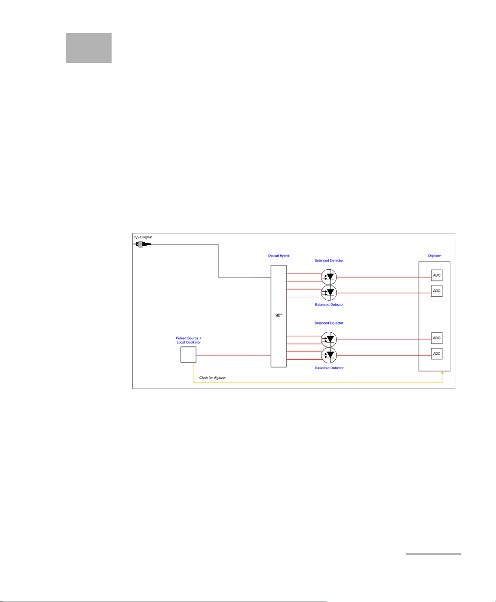
C Coherent Detection and Sampling Methods .......................................... 239

Coherent Detection .............................................................................................................239

Sampling Methods .............................................................................................................240

PSO-200 Principles of Operation .........................................................................................242

Signal Processing Algorithms ..............................................................................................244

D Modulation Schemes ............................................................................... 247

E Measurement Definitions ........................................................................ 251

Data Used for Measurements .............................................................................................251

Measurements for Constellation Charts ..............................................................................252

Measurements for Eye Diagrams ........................................................................................258

Index .............................................................................................................. 267

Optical Modulation Analyzer v

Certification Information

North America Regulatory Statement

This unit was certified by an agency approved in both Canada and the United States of America. It has been evaluated according to applicable North American approved standards for product safety for use in Canada and the United States.

Electronic test and measurement equipment is exempt from FCC part 15, subpart B compliance in the United States of America and from ICES-003 compliance in Canada. However, EXFO Inc. makes reasonable efforts to ensure compliance to the applicable standards.

The limits set by these standards are designed to provide reasonable protection against harmful interference when the equipment is operated in a commercial environment. This equipment generates, uses, and can radiate radio frequency energy and, if not installed and used in accordance with the user guide, may cause harmful interference to radio communications. Operation of this equipment in a residential area is likely to cause harmful interference in which case the user will be required to correct the interference at his own expense.

Modifications not expressly approved by the manufacturer could void the user's authority to operate the equipment.

IMPORTANT

Use of shielded remote I/O cables, with properly grounded shields and metal connectors, is recommended in order to reduce radio frequency interference that may emanate from these cables.

vi PSO-200

Certification Information

Application of Council Directive(s): 2006/95/EC - The Low Voltage Directive 2004/108/EC - The EMC Directive 2006/66/EC - The Battery Directive 93/68/EEC - CE Marking And their amendments Manufacturer’s Name: EXFO Inc. Manufacturer’s Address: 400 Godin Avenue Quebec, Quebec Canada, G1M 2K2 (418) 683-0211 Equipment Type/Environment: Test & Measurement / Industrial Trade Name/Model No.: PSO-200 / Optical Modulation Analyzer

Standard(s) to which Conformity is Declared:

EN 61010-1:2001 Edition 2.0 Safety Requirements for Electrical Equipment for Measurement,

Control, and Laboratory Use, Part 1: General Requirements.

EN 61326-1:2006 Electrical Equipment for Measurement, Control and Laboratory

Use - EMC Requirements – Part 1: General requirements

EN 60825-1:2007 Edition 2.0 Safety of laser products – Part 1: Equipment classification,

requirements, and user’s guide

EN 55022: 2006 + A1: 2007 Information technology equipment - Radio disturbance

characteristics - Limits and methods of measurement

I, the undersigned, hereby declare that the equipment specified above conforms to the above Directive and Standards.

Manufacturer

Signature:

Full Name: Stephen Bull, E. Eng

Position: Vice-President Research and

Development

Address: 400 Godin Avenue, Quebec (Quebec),

Canada, G1M 2K2

Date: August 17, 2010

DECLARATION OF CONFORMITY

European Community Declaration of Conformity

Optical Modulation Analyzer vii

1 Introducing the PSO-200

Optical Modulation Analyzer

As new advanced modulation schemes enable the transmission of high-speed optical signals over fiber, research centers, network equipment manufacturers and eventually carriers need new test instruments to properly characterize these signals.

Main Features

The PSO-200 Optical Modulation Analyzer uses equivalent-time optical sampling, allowing the complete characterization of random or repetitive digital signals at 100 Gb/s, 400 Gb/s, 1 Tb/s and beyond.

The PSO-200 displays constellation charts, eye diagrams and patterns with very high temporal resolution. It is a useful tool to study and characterize very high bit-rate systems or very fast events like short pulses, where the bandwidth of ordinary electrical sampling oscilloscopes is not sufficient.

The PSO-200 can measure a number of modulation formats: OOK, BPSK, APSK, QPSK and 16-QAM, all in return-to-zero (RZ) or non-return-to-zero (NRZ) formats.

Optical Modulation Analyzer 1

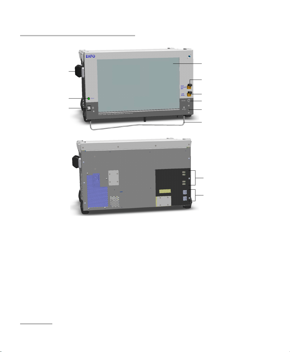
Introducing the PSO-200 Optical Modulation Analyzer

Local oscillator input port

Input signal port

Trigger port

USB port

Power button

Remote control

indicator/Return

to local mode

Handle

Touchscreen

Support

LAN ports

USB ports

Main Features

The PSO-200 Optical Modulation Analyzer has the following features:

 Fully customizable display layout and selection of graphs (intensity,

phase, error-vector magnitude) in eye diagram and pattern modes.

 Analysis tools such as averaging, masks, filters and advanced signal

processing algorithms.

 Post-processing tools (acquisition import and export, reanalysis with

different settings, offline application).

2 PSO-200

 Bit pattern customization with the Gearbox

 Remote control available (Ethernet TCP/IP with SCPI commands).

Introducing the PSO-200 Optical Modulation Analyzer

Conventions

Before using the product described in this guide, you should understand the following conventions:

WARNING

Indicates a potentially hazardous situation which, if not avoided, could result in death or serious injury. Do not proceed unless you understand and meet the required conditions.

CAUTION

Indicates a potentially hazardous situation which, if not avoided, may result in minor or moderate injury. Do not proceed unless you understand and meet the required conditions.

CAUTION

Indicates a potentially hazardous situation which, if not avoided, may result in component damage. Do not proceed unless you understand and meet the required conditions.

Conventions

IMPORTANT

Refers to information about this product you should not overlook.

Optical Modulation Analyzer 3

2 Safety Information

Laser Safety Information

WARNING

Do not install or terminate fibers while a light source is active. Never look directly into a live fiber and ensure that your eyes are protected at all times.

WARNING

The use of controls, adjustments and procedures other than those specified herein may result in exposure to hazardous situations or impair the protection provided by this unit.

IMPORTANT

When you see the following symbol on your unit , make sure that you refer to the instructions provided in your user documentation. Ensure that you understand and meet the required conditions before using your product.

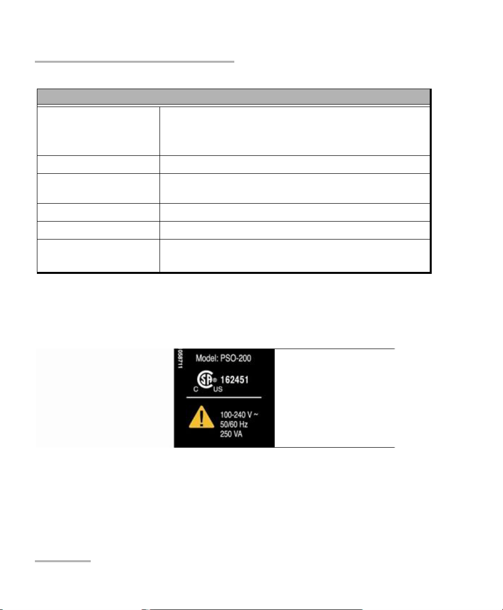
Your instrument is a Class 1 laser product in compliance with standards IEC 60825-1 2007 and 21 CFR 1040.10. Laser radiation may be encountered at the output port.

The following label indicates that a product contains a Class 1 source:

Note: The label is located at the back of the unit.

Optical Modulation Analyzer 5

Safety Information

Electrical Safety Information

This unit uses an international safety standard three-wire power cable. This cable serves as a ground when connected to an appropriate AC power outlet.

Note: To ensure that the unit is completely turned off, disconnect the power cable.

WARNING

 Insert the power cable plug into a power outlet with a

protective ground contact. Do not use an extension cord without a protective conductor.

 Before turning on the unit, connect all grounding terminals,

extension cords and devices to a protective ground via a ground socket. Any interruption of the protective grounding is a potential shock hazard and may cause personal injury. Whenever the ground protection is impaired, do not use the unit and secure it against any accidental operation.

 Do not tamper with the protective ground terminal.

6 PSO-200

Safety Information

Electrical Safety Information

The color coding used in the electric cable depends on the cable. New plugs should meet the local safety requirements and include:

 adequate load-carrying capacity

 ground connection

 cable clamp

WARNING

 Use this unit indoors only.

 Position the unit so that the air can circulate freely around it.

 Do not remove unit covers during operation.

 Operation of any electrical instrument around flammable gases

or fumes constitutes a major safety hazard.

 To avoid electrical shock, do not operate the unit if any part of

the outer surface (covers, panels, etc.) is damaged.

 Only authorized personnel should carry out adjustments,

maintenance or repair of opened units under voltage. A person qualified in first aid must also be present. Do not replace any components while power cable is connected.

 Capacitors inside the unit may be charged even if the unit has

been disconnected from its electrical supply.

Optical Modulation Analyzer 7

Safety Information

Electrical Safety Information

Tem pe ra tu re

 Operation

 Storage

Relative humidity

Equipment Ratings

0 °C to 35 °C (32 °F to 95 °F)

-40 °C to 70 °C (-40 °F to 158 °F)

80 % non-condensing

Maximum operation

2000 m (6562 ft)

altitude

Pollution degree 2

Installation category II

Powe r supp l y rati ng

100 V to 240 V (50 Hz/60 Hz)

maximum input power 250 VA

a. Measured in 0 °C to 31 °C (32 °F to 87.8 °F) range, decreasing linearly to 50 % at 40 °C (104 °F).

b. Not exceeding ± 10 % of the nominal voltage.

The following label is located on the back panel of the unit:

8 PSO-200

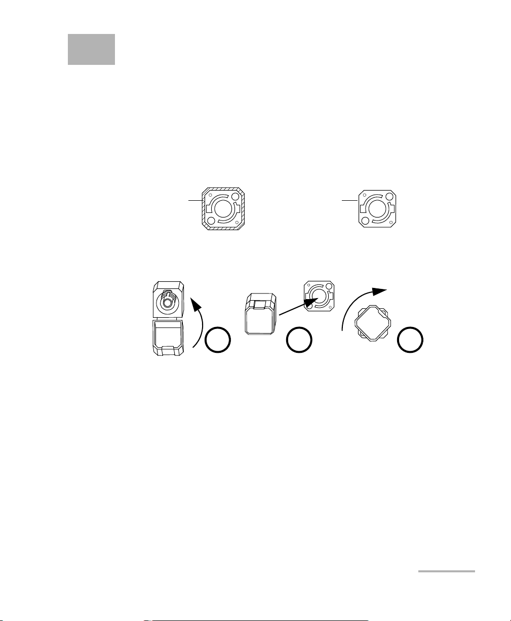
3 Getting Started with Your

Bare metal

(or blue border)

indicates UPC

option

Green border indicates APC

option

2 3 4

Optical Modulation Analyzer

Installing the EXFO Universal Interface (EUI)

The EUI fixed baseplate is available for connectors with angled (APC) or non-angled (UPC) polishing. A green border around the baseplate indicates that it is for APC-type connectors.

To install an EUI connector adapter onto the EUI baseplate:

1. Hold the EUI connector adapter so the dust cap opens downwards.

2. Close the dust cap in order to hold the connector adapter more firmly.

3. Insert the connector adapter into the baseplate.

4. While pushing firmly, turn the connector adapter clockwise on the

baseplate to lock it in place.

Optical Modulation Analyzer 9

Getting Started with Your Optical Modulation Analyzer

Cleaning and Connecting Optical Fibers

IMPORTANT

To ensure maximum power and to avoid erroneous readings:

 Always inspect fiber ends and make sure that they are clean as

explained below before inserting them into the port. EXFO is not responsible for damage or errors caused by bad fiber cleaning or handling.

 Ensure that your patchcord has appropriate connectors. Joining

mismatched connectors will damage the ferrules.

To connect the fiber-optic cable to the port:

1. Inspect the fiber using a fiber inspection microscope. If the fiber is

clean, proceed to connecting it to the port. If the fiber is dirty, clean it as explained below.

2. Clean the fiber ends as follows:

2a. Gently wipe the fiber end with a lint-free swab dipped in isopropyl

alcohol.

2b. Use compressed air to dry completely.

2c. Visually inspect the fiber end to ensure its cleanliness.

10 PSO-200

Getting Started with Your Optical Modulation Analyzer

Cleaning and Connecting Optical Fibers

3. Carefully align the connector and port to prevent the fiber end from touching the outside of the port or rubbing against other surfaces.

If your connector features a key, ensure that it is fully fitted into the port’s corresponding notch.

4. Push the connector in so that the fiber-optic cable is firmly in place, thus ensuring adequate contact.

If your connector features a screwsleeve, tighten the connector enough to firmly maintain the fiber in place. Do not overtighten, as this will damage the fiber and the port.

Note: If your fiber-optic cable is not properly aligned and/or connected, you will

notice heavy loss and reflection.

EXFO uses good quality connectors in compliance with EIA-455-21A standards.

To keep connectors clean and in good condition, EXFO strongly recommends inspecting them with a fiber inspection probe before connecting them. Failure to do so will result in permanent damage to the connectors and degradation in measurements.

Optical Modulation Analyzer 11

Getting Started with Your Optical Modulation Analyzer

Starting and Exiting the Optical Modulation Analyzer Application

The PSO-200 Optical Modulation Analyzer runs on a Microsoft Windows environment. When you turn it on, the unit should automatically start the Optical Modulation Analyzer application.

When starting the application, the PSO-200 requires some time to initialize, during which certain features, such as the Start button, are not available. A message is displayed in the status bar while initialization is in progress.

To start the application:

 Double-click the shortcut icon on the desktop.

 From the Windows Start menu, select All Programs > EXFO >

Optical Modulation Analyzer.

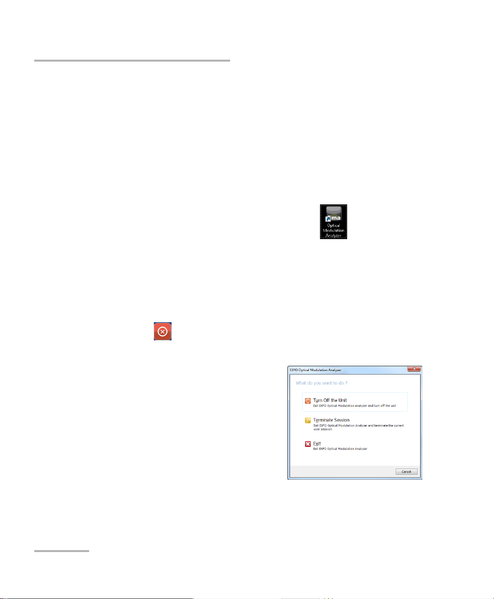
To exit the application:

1. From the File menu, select Exit.

Click the button in the bottom right corner of the main window.

2. Select which shutdown method you want.

 Turn off the unit: closes the

application and completely shuts down the PSO-200.

 Terminate session: closes the

application and logs off the current Windows session, but does not shut down the PSO-200.

 Exit: closes the application only.

Note: If there were unsaved acquisitions, you will be prompted to save them

when you exit the application.

12 PSO-200

4 Setting Up the Optical

Modulation Analyzer

You should start by setting parameters on the PSO-200 so that acquisitions are performed according to the signal you are analyzing and that the results meet your needs.

You can also change some settings during an acquisition, or even afterwards to see how it would have affected the results. See Reanalyzing Acquisitions with New Settings on page 115.

Note: Changing settings during an acquisition will not stop it. However, acquired

bursts will be cleared and new bursts will be taken using the new settings.

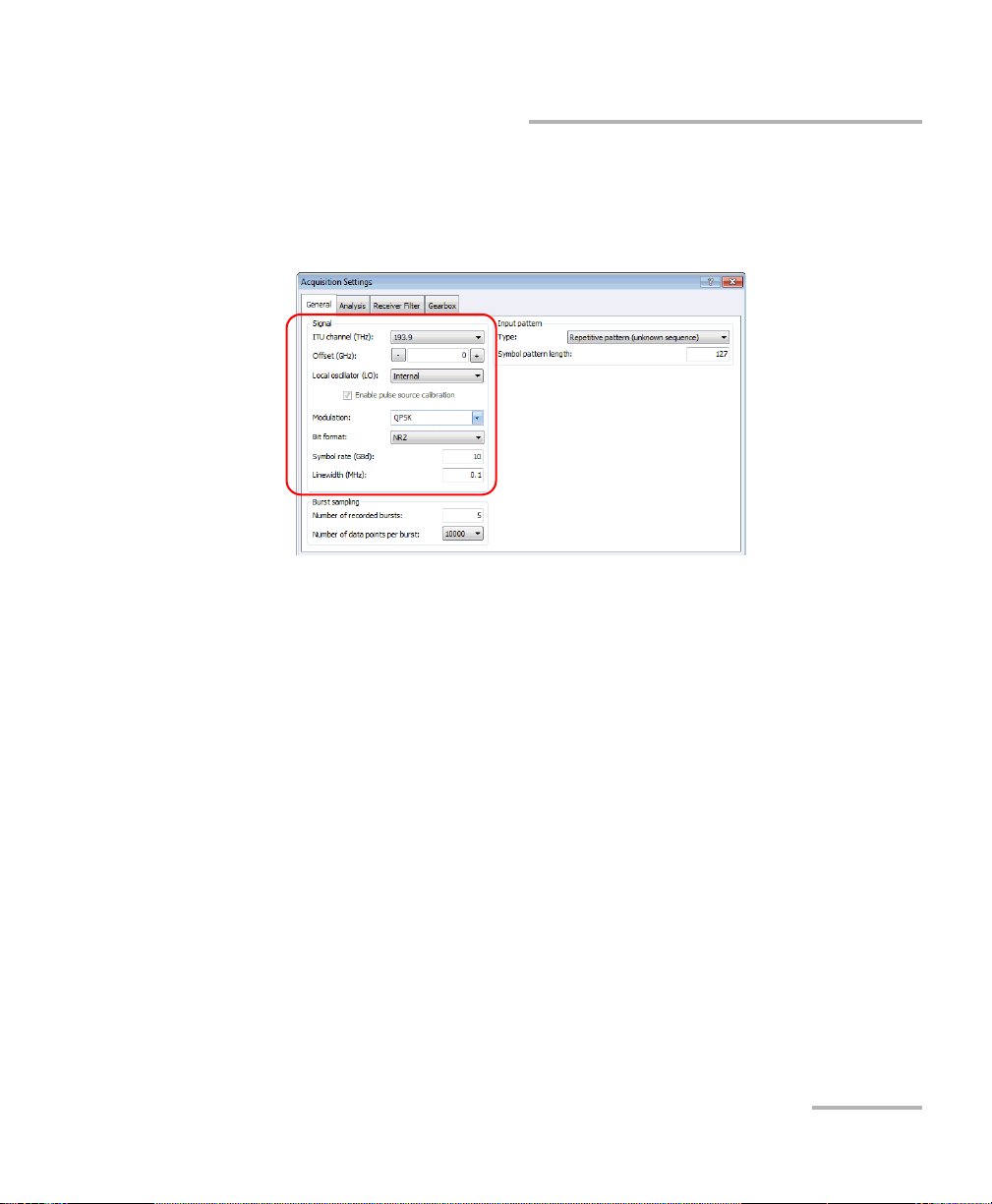
Configuring the Input Signal

You will need to provide the following information about your input signal, in order to obtain relevant results:

 ITU channel and Offset: this is the signal frequency or wavelength. You

can select a channel from the ITU grid (25 GHz spacing), and if needed, indicate an offset value of up to half the channel.

The signal spectrum needs to be within the receiver spectrum (see Technical Specifications on page 131), otherwise the constellation chart might be distorted and noisy, or even not visible at all.

 Local oscillator: you can use the PSO-200’s internal pulsed laser source

or your own external laser source. For explanations on when and how to use an external source, see Using an External Local Oscillator on page 27).

 Modulation scheme (DPSK, QPSK, etc.): select the scheme according

to the modulation of your signal under test. Dual-polarization signals are prefixed with “DP” See Modulation Schemes on page 247.

The Free-Run, CW and Intensity Sampling modes allow bypassing some signal processing algorithms for troubleshooting or other analysis purposes. See Using Special Modulation Modes on page 24.

Optical Modulation Analyzer 13

Setting Up the Optical Modulation Analyzer

Configuring the Input Signal

 Bit format (RZ or NRZ): this should be used according to the pulse

carving status of your signal under test (RZ for pulse-carved signals, NRZ otherwise, as explained in Modulation Schemes on page 247). This setting affects measurements associated with the waveform.

 Symbol rate (in GBd): symbol rate of the input signal. An accurate rate

(±0.05 GBd or better) is needed to recover the correct waveform (via pattern synchronization) and to get valid time-domain measurements from the time reconstruction algorithms (see Sampling Methods on page 240).

 Linewidth: controls the speed of the IF tracking algorithm and should

correspond to the signal source’s linewidth (approximately ±0.25 MHz).

If it is set too low, there will be remaining phase noise on the captured waveform (constellation symbols spread in the phase direction) or even the phase will not be accurately tracked (cycle slips will occur).

If it is set too high, the algorithm will remove phase noise not originating from the signal source (constellation symbols will be compressed in the phase direction).

A proper setting balances these two conditions (equal noise in both amplitude and phase, or a constellation with symmetric points).

14 PSO-200

Setting Up the Optical Modulation Analyzer

Configuring the Input Signal

To configure the input signal type and properties:

1. From the Settings menu, select Acquisition.

2. Under the General tab, enter the settings in the Signal section.

3. Click Apply to confirm your settings, or OK to also close the window.

Optical Modulation Analyzer 15

Setting Up the Optical Modulation Analyzer

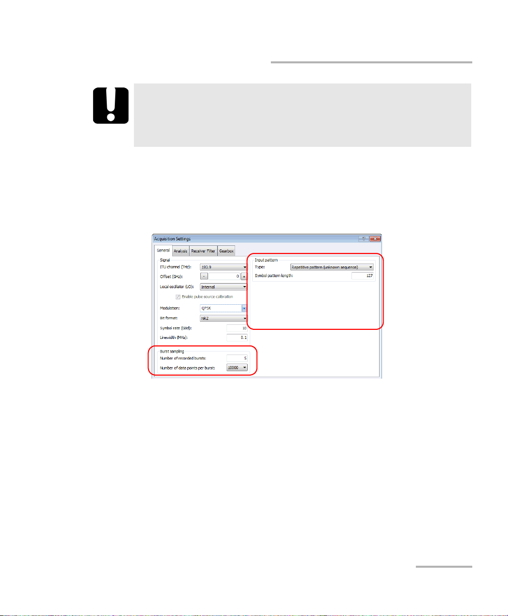
Setting Other Acquisition Parameters

Use the following parameters to improve the recovered waveform:

 Burst sampling parameters: you can specify the number of bursts that

will be recorded or buffered by the application, as well as the number of data points in each burst. A larger number of points will take more time to process but provide better results.

 Input pattern mode and parameters: available modes depend on the

selected modulation scheme.

 Random – if random signals (live traffic or framed PRBS) or very

long patterns (2

-1 PRBS) are used. The constellation chart and eye diagrams of amplitude and phase can be measured, but not the patterns. No filtering, averaging or CD unwrapping possible.

 Repetitive (unknown pattern) – if your signal under test comprises

a repetitive pattern with known word length (for example, PRBS with header data). The pattern can also be recovered.

 User-defined symbol pattern – if you know exactly the symbol

pattern or can extract it from an acquisition (such as in Repetitive mode or if your modulation scheme is not supported by the PSO-200). This mode improves signal processing algorithms and allows the calculation of a symbol error rate (SER). For details, see Importing User-Defined Symbol Patterns on page 84.

 PRBS – if your signal is generated from pseudo-random binary

sequences. Since the pattern is known, you can obtain bit error rate (BER) information and you can use the Gearbox to fine-tune the bit alignment of your signal stream.

 User-defined bit pattern – if you know exactly the sequence of bits

in your signal. As for PRBS, you can obtain the BER and are able to use the Gearbox.

Note: Free-Run, CW and Intensity Sampling signals do not allow patterns.

16 PSO-200

Setting Up the Optical Modulation Analyzer

Setting Other Acquisition Parameters

IMPORTANT

Make sure a pattern can be displayed (magnitude graph) in any of the pattern mode acquisitions. If pattern synchronization cannot be achieved, switch the input pattern type to Random.

To set the acquisition parameters:

1. From the Settings menu, select Acquisition.

2. Under the General tab, enter the settings for the burst sampling and

input pattern.

3. If you have selected Repetitive pattern (unknown sequence), simply

enter the Symbol pattern length.

Otherwise, proceed as explained in Bit Pattern Analysis and the Gearbox on page 79.

4. Click Apply to confirm your settings, or OK to also close the window.

Optical Modulation Analyzer 17

Setting Up the Optical Modulation Analyzer

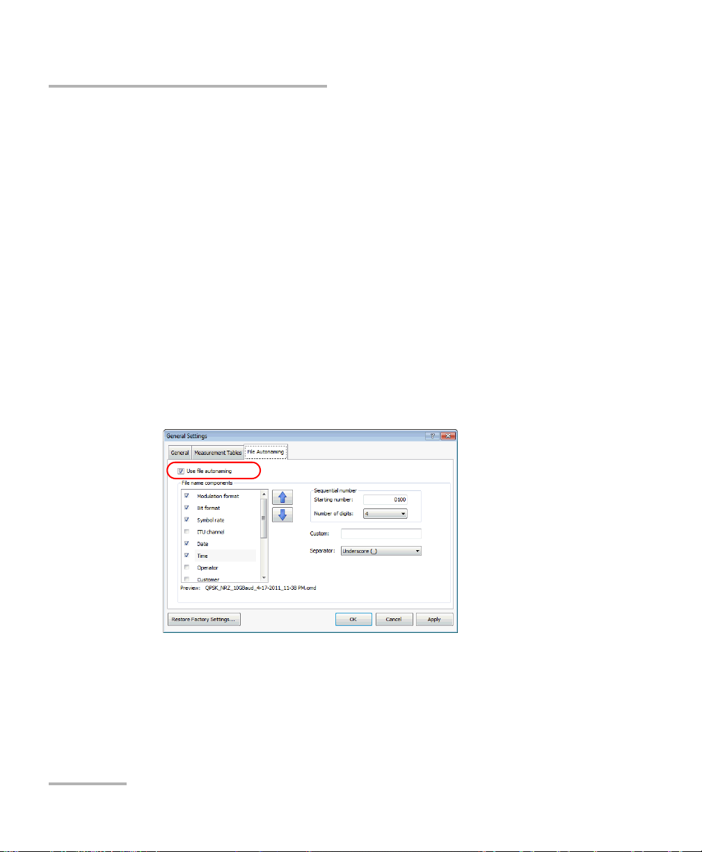
Setting File Autonaming

Autonaming helps you create a predefined file naming scheme for future saved acquisitions. This can include data components, date/time and

sequential numbering. This way you are sure not to overwrite your previous files and always follow a standard that is meaningful to you.

Note: Characters that cannot be used in a file name are replaced by a tilde “~”.

Note: Path and file names combined cannot exceed 260 characters. If the items

you have selected lead to a name that is too long, it will be truncated.

To define and activate the autonaming scheme:

1. From the Settings menu, select General.

2. Select the File Autonaming tab.

3. Check the box to enable the option if you want to use autonaming.

18 PSO-200

Setting Up the Optical Modulation Analyzer

Setting File Autonaming

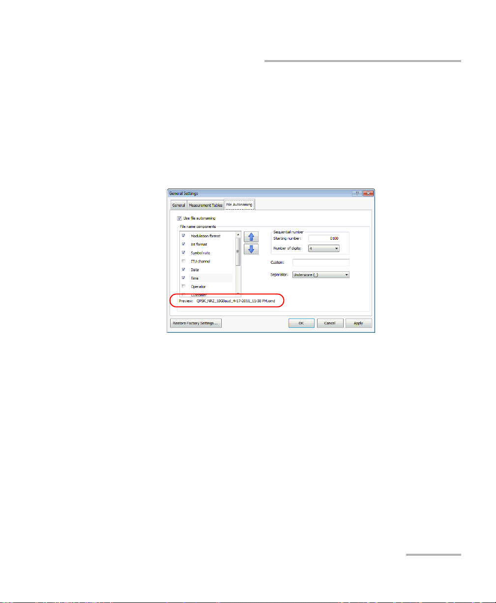
4. Define the autonaming scheme. A sample file name shows you the

final output.

 Select data components you want to include in the name. You

must select at least one item in the list. You can change the order using the up and down arrow buttons.

Note: The order of the items is kept until you revert to the factory settings.

 Set the sequential number values. You can enter the starting

number and select how many digits are to be used. Once the sequence reaches the maximum value (for example, 999 for a 3-digit sequence), the sequence is reset to the first value.

 If desired, you can include a comment for your file name in the

Custom box. The comment contains up to 100 characters.

 Select a separator value to place between the selected data

components.

5. Click Apply to confirm your settings, or OK to also close the window.

Optical Modulation Analyzer 19

Setting Up the Optical Modulation Analyzer

Identifying Acquisitions

Setting up acquisition information can save you time and work, as your acquisitions will be identified according to your needs each time. You can either set default information for future acquisitions (especially useful in conjunction with file autonaming in automated production environments), or add specific information for the current acquisition.

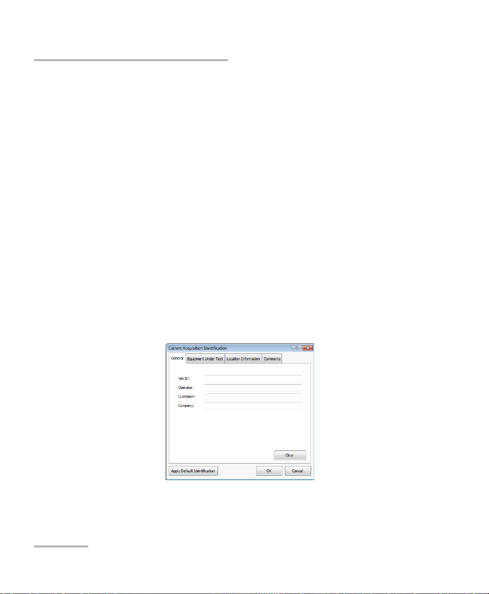
To enter acquisition identification:

1. If you want to set the default information, from the Settings menu,

select Default Acquisition Identification.

If you want to identify the current acquisition only, from the File menu, select Properties, then Current Acquisition Identification.

Note: When editing current acquisition details, you can click Apply Default

Identification in any tab to insert the default data.

2. Select the General tab, then fill out the basic information for your acquisition, such as the operator or customer name.

20 PSO-200

Setting Up the Optical Modulation Analyzer

Identifying Acquisitions

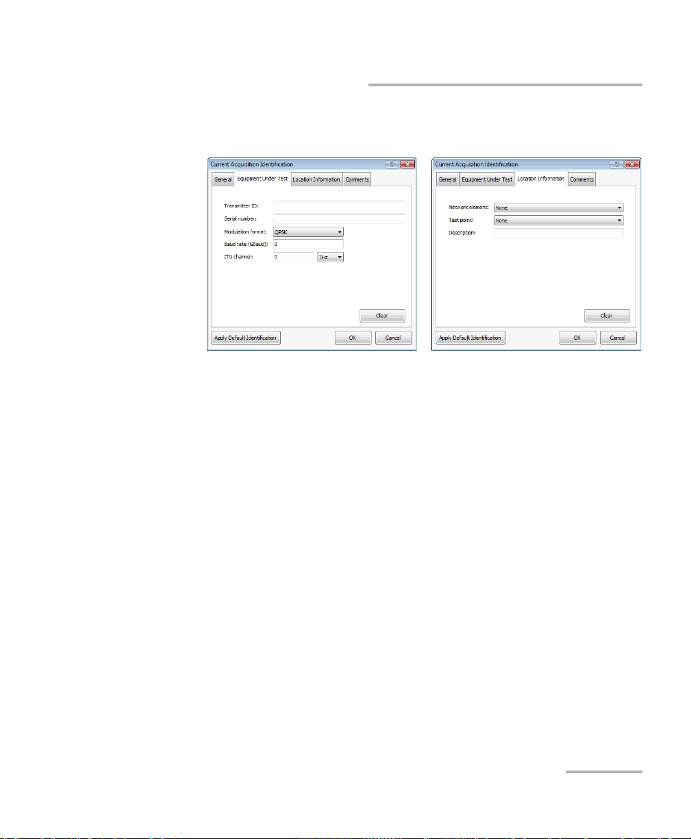
3. Select the Equipment Under Test and Location Information tabs and provide details that pertain to your specific test case.

You can also add a personalized comment in the Comments tab.

4. Click Apply to confirm your settings, or OK to also close the window.

Optical Modulation Analyzer 21

Setting Up the Optical Modulation Analyzer

Setting Analysis Parameters

The signal can be analyzed while being acquired or afterwards in reanalysis mode. The following tools are available.

 Burst averaging (see Using Averaging to Improve Results on page 70).

 Measurement windows:

 Data – time range defined as percentages of the symbol period, as

explained in Distinguishing Data Points from Transitions on page 62.

 Amplitude – intensity range defined as percentages of the eye

amplitude, as explained in Measurements for Eye Diagrams on page 258. It is used to compute values like “rise” and “fall” times and provides the eye height.

 Specific optional signal processing algorithms (see Applying Advanced

Signal Processing Algorithms on page 72). Available algorithms depend

on the selected modulation format.

 Pattern masks to test the quality of the signal and perform quick

pass/fail analysis (see Using Pattern Masks on page 64).

22 PSO-200

Setting Up the Optical Modulation Analyzer

Setting Analysis Parameters

To set the analysis parameters:

1. From the Settings menu, select Acquisition.

2. Under the Analysis tab, select the desired analysis options.

3. Click Apply to confirm your settings, or OK to also close the window.

Optical Modulation Analyzer 23

Setting Up the Optical Modulation Analyzer

Using Special Modulation Modes

In some situations, when the input signal does not represent phase-encoded data, it can be valuable to bypass some of the signal processing algorithms to visualize the signal with a better refresh rate or under different conditions. For example, it may be useful to study just the intensity before a phase-encoding transmitter is set up correctly, for debugging purposes.

You can also export the signal data obtained when bypassing some algorithms to analyze with your own tools (such as MATLAB algorithms).

The Optical Modulation Analyzer application offers the following modes:

Mode Usage

Free-run General debugging, oscilloscope-like behavior;

useful in initial connections to ensure signal input

Continuous wave CW laser analysis, analyze phase noise

Intensity sampling Fast, useful for a first tuning of the system under test,

shows waveform envelope

Here are the signal processing algorithms (applied or optional) for each mode (for details, see Signal Processing Algorithms on page 244):

Signal Processing Algorithms

(in order)

Free-Run CW

Intensity

Sampling

Polarization demultiplexing Optional Optional Optional

Time reconstruction vector – – Applied

Intermediate frequency recovery – Optional –

Alignment –––

Other algorithms – Applied –

24 PSO-200

Setting Up the Optical Modulation Analyzer

Using Special Modulation Modes

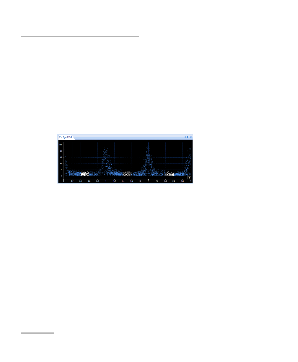
The figure below shows an example of intensity sampling of 42 GBd QPSK data (top: intensity eye diagram; bottom: corresponding 127 bit pattern). The intermediate frequency recovery algorithm is bypassed so that only intensity is sampled. The phase information is not retrieved.

Optical Modulation Analyzer 25

Setting Up the Optical Modulation Analyzer

Using Special Modulation Modes

To select a special modulation mode and activate optional algorithms:

1. From the Settings menu, select Acquisition.

2. Under the General tab, select the special mode in the Modulation list.

3. Under the Analysis tab, select the desired signal processing algorithms

to apply.

4. Click Apply to confirm your settings, or OK to also close the window.

26 PSO-200

Setting Up the Optical Modulation Analyzer

Using an External Local Oscillator

The External local oscillator (LO) option allows you to use your own laser as a source for the local oscillator instead of the PSO-200 internal laser. This is useful in the following cases:

 When your signal source has an extremely low phase noise, such that

the overall phase noise becomes dominated by the internal LO source.

If you use as LO a laser source with equivalent (or better) phase noise characteristics, you can reduce the total phase noise in acquisitions.

 To accomplish self-homodyne measurements by using the same laser

source split between the signal and LO, offering identical phase noise characteristics on both.

In order to cancel the influence of the source phase noise on the measurements, and thus not requiring phase tracking, you must ensure that the delays of the signal and LO paths will match precisely (even more when your laser source has wider linewidth).

The external laser source must meet the specified power range (see Technical Specifications on page 131) and must use polarization-maintaining fiber (PMF).

When the external LO source is distinct from the signal source:

 The ITU Channel parameter also applies to the external LO source, so

both sources must have the same frequency/wavelength.

 The Linewidth parameter should be set to the wider laser source.

Optical Modulation Analyzer 27

Setting Up the Optical Modulation Analyzer

Using an External Local Oscillator

By default, the application automatically calibrates the external LO source during acquisitions. You can disable this option, but you should only do so if the application requires it (see message below), in which case the application will try to use the last calibration values obtained with the internal LO.

Note: Changing the frequency/wavelength or symbol rate will clear the

calibration values, thus requiring the above procedure.

28 PSO-200

Setting Up the Optical Modulation Analyzer

Using an External Local Oscillator

To enable the external local oscillator:

1. From the Settings menu, select Acquisition.

2. Under the General tab, select External in the Local oscillator list.

Optical Modulation Analyzer 29

Setting Up the Optical Modulation Analyzer

Using an External Local Oscillator

3. If necessary only, disable the automatic calibration by clearing the

Enable pulse source calibration box.

4. Click Apply to confirm your settings, or OK to also close the window.

5. Connect your external laser source to the Local Oscillator Input port

on the PSO-200 front panel.

6. Start an acquisition.

IMPORTANT

If you revert to Internal LO, ensure your external source is disconnected before clicking Start for the next acquisition.

30 PSO-200

Setting Up the Optical Modulation Analyzer

Locking the Remote Unit

If you control the unit remotely, you can set it so that the keyboard, mouse and touchscreen are inactive. This can be useful when you do not want someone to accidently change your settings.

To lock the unit when using remote control:

1. From the main window, select the Settings menu, then General.

2. Select the General tab.

3. Under SCPI, select the option to lock the unit.

The lock takes effect when you start the remote communication. You can unlock the unit via remote control or using the return to local button on the front of the unit.

Optical Modulation Analyzer 31

5 Performing Acquisitions

Starting and Stopping an Acquisition

Once you start an acquisition, it will continue until you stop it. If you had a previous acquisition that you have not saved, you will be prompted to save it before starting a new one.

While an acquisition is in progress, the on-screen data and graphs are updated upon each burst, and you can still change the display layout. However, you cannot use the playback controls, or open or save files.

To start an acquisition:

Press the Start button.

From the Measurement menu, select Start.

To stop an acquisition:

While the acquisition is in progress, press the Stop button.

From the Measurement menu, select Stop.

Note: Closing the application will also stop the acquisition.

Optical Modulation Analyzer 33

Performing Acquisitions

Clearing Data During an Acquisition

While an acquisition is in progress, you can clear the data already acquired at any time in order to capture a clean signal without the glitches that might have been introduced during manipulations.

All graphs and measurement tables are reset, and burst count restarts at 1. The Y axis is re-scaled to a normalized unit.

To clear acquired data:

While an acquisition is in progress, press the (Clear) button.

From the Measurement menu, select Clear Data.

34 PSO-200

Performing Acquisitions

Saving Acquisitions to a File

Once an acquisition is completed, you can save it for later analysis and playback.

You can set a default folder to use for future acquisitions. The application offers you to save the file in this folder, but you can always select a different location.

Note: If autonaming was enabled (see Setting File Autonaming on page 18), the

application will suggest an appropriate name, but you can change it.

To set a default folder for your saved files:

1. From the Settings menu, select General.

2. Select the General tab.

3. Under Storage, locate the folder you want using the Browse button.

4. Click Apply to confirm your settings, or OK to also close the window.

To save an acquisition file:

1. From the File menu, select Save As.

2. Navigate to the folder where you want to save the file.

3. Click Save.

If you had previously saved the file, you can use Save instead of Save As to automatically save it with its current name and location. You can also use the button on the main window.

Optical Modulation Analyzer 35

Performing Acquisitions

Ready Ready Ready Ready Ready Ready

Tri g

Burst

Analysis

Triggered acquisition (1 burst/trig)

Ready

Tri g

Burst

Analysis

Triggered acquisition (6 bursts/trig)

Ready

Tri g

Burst

Analysis

Triggered acquisition (6 bursts/trig, trigs too fast)

12 3456 123

Activating Trigger-Based Acquisitions

You could use an external equipment, such as a BER tester, to initiate burst acquisitions on the PSO-200 based on trigger signals. This can be useful in automated long-term tests.

When you start this acquisition process, the application will be on hold, waiting for a trigger signal (which can occur hours later) to acquire new bursts as specified. This process will stop if you press the Stop button or when it reaches the specified number of trigs.

If the external trig signal occurs while the previous burst is still being acquired, the PSO-200 will ignore this trig signal and wait for the next one.

Note: You must stop the trigger-based acquisition in order to change its settings.

36 PSO-200

Performing Acquisitions

Activating Trigger-Based Acquisitions

To activate triggered acquisitions:

1. From the Settings menu, select Acquisition.

2. Under the Gate Acquisition tab, select Acquire a burst when

receiving a signal....

3. Select the trigger parameters as follows:

 Number of recorded bursts: bursts buffered in memory, overriding

the equivalent setting in the General tab.

 Number of bursts to acquire per trig event

 Stop acquisition after N trig events: will stop after this number of

“useful” trigs (trigs leading to a burst acquisition, not counting skipped trigs).

 Save to file after stopping the acquisition: the acquisition will be

saved in the location (path) specified in General Settings, using autonaming if enabled (or generic names “OMDFileX.omd” otherwise). A file can contain at most 140 bursts.

 Trig signal: select whether to use the rising signal (reaching 2.5 V

upwards) or the falling signal (reaching 2.5 V downwards).

4. Click Apply to confirm your settings, or OK to also close the window.

5. Connect your external equipment to the Trigger port on the PSO-200

front panel.

6. Press the Start button. The application will wait for the trigger signal.

Optical Modulation Analyzer 37

6 Customizing the Graph and

Split bars

Data Layout

Selecting and Customizing the Layout

The application’s main window is fully customizable. You can start with one of the preset single- or dual-polarization layouts that may already suit your needs. Each layout contains a set of graphs and tables.

Note: Predefined layouts are not editable. Once you close a tab, you can only

make it appear again by re-selecting a layout that contains it.

Note: Dual-polarization layouts are available even if your unit does not support it,

allowing you to open files previously acquired on other units. Polarizations are identified by X and Y.

Optical Modulation Analyzer 39

Customizing the Graph and Data Layout

Selecting and Customizing the Layout

At any time during of after acquisitions, you can change the displayed graphs (except the constellation), resize the tabs or close those you do not want to see. The application will remember your layout for your next work session.

Available graphs in the Optical Modulation Analyzer application are described later in this chapter.

To select a predefined layout:

1. From the Display menu, select Layout.

2. Select which layout better suits your situation. You can also use the

keyboard shortcuts.

To change the graph on a tab (eye or pattern):

1. Right-click on the graph tab for which you want to change the content.

Select the graph tab, then in the Display menu, select Graph Type.

2. Select a new type of graph to display.

To r es i ze a t ab :

Use the split bars enclosing the tab you want to resize.

To close a tab:

Click the button in the upper right corner of the tab.

To change the displayed polarization:

1. From the Display menu, select Polarization.

2. Select the polarization (X or Y) to display on all graphs and tables.

Note: The Polarization option is only available if you are viewing a

dual-polarization signal on a single-polarization layout.

40 PSO-200

Customizing the Graph and Data Layout

}

“Q”

“I”

Symbol

I-Value

Q-Value



Polar-to-Rectangular Conversion

Project signal to

“I” and “Q” axes

Constellation Chart

Useful when characterizing advanced modulation schemes such as DP-QPSK, the constellation chart is a representation of a signal modulated in phase and/or in amplitude.

It shows valid symbols (amplitude and phase relative to the carrier) of a modulation format on a polar graph. Since each symbol is encoded with n bits (depending on the modulation scheme), there will be 2 symbols.

permitted

The “I” axis (in-phase) represents the “real” part of the complex field, while the “Q” axis (quadrature) represents the “imaginary” part.

The length of the vector to the symbol in the chart is the amplitude of the signal (normalized in the Optical Modulation Analyzer application), and its angle from the “I” axis is the phase of the signal.

Note: There is one constellation chart per polarization state (X and Y).

Optical Modulation Analyzer 41

Customizing the Graph and Data Layout

Constellation point

Tra nsit ions

Constellation Chart

The figure below shows an example of a QPSK constellation with four points (2-bit symbols) comprising the data-carrying signal. No time information is given since it would be on the z axis.

Transitions between constellation points contribute significantly to the spectral content of the input signal, and hence the optimization of these transitions is often the most critical aspect of transmitter operation. Consequently, the PSO-200 is designed to not only display the constellation points, but also visualize these transitions with high accuracy.

If the signal is without error, the ideal symbol would appear as a single point on the constellation. However, signal impairments and modulation errors cause deviations and the symbols will show as a group of points dispersed around the ideal location.

For details about the measurements derived from the constellation chart, see Measurements for Constellation Charts on page 252.

42 PSO-200

Customizing the Graph and Data Layout

Symbol period

Eye Diagrams

An eye diagram is a trace of the intensity, magnitude, or phase, as a function of time, where the corresponding time vector has been “folded” to an integer number of symbol periods (see Equivalent-Time Sampling on page 241).

Traditionally, intensity (power) has been shown in eye diagrams, since the power itself contains the information in on-off keying (OOK) data modulation. With more complex phase-encoded signals with coherent detection, I/Q amplitude and phase are also shown in eye diagrams.

To acquire the eye diagram, the PSO-200 relies on a time reconstruction algorithm that works like a software-based clock recovery.

Note: All eye diagrams are normalized on the Y-axis.

Several system performance measures can be derived by analyzing the eye diagram. It allows you to determine whether the signal exhibits excessive jitter or noise, or if it is too slow to change, or displays unacceptable overshoot. Distortion of the signal waveform due to inter-symbol interference (ISI) and noise appears as closure of the eye diagram.

For details about the measurements derived from the eye diagrams, see Measurements for Eye Diagrams on page 258.

Optical Modulation Analyzer 43

Customizing the Graph and Data Layout

ItB() ReE tB()()=

() ImE tB()()=

NRZ-QPSK data

QPSK data

Eye Diagrams

I/Q Eye Diagrams

The I (in-phase) and Q (quadrature) eye diagrams represent the “real” and “imaginary” parts of the complex field as a function of time, respectively.

where t

is the remainder after division with the symbol period .

The I eye diagram can be seen as the data visible by looking from the right of the constellation chart. Similarly with the Q eye diagram by looking from the top.

Phase Eye Diagram

Eye diagram of arg(E(tB)). No amplitude information is provided.

This graph shows the different phases of the signal and the transitions. Its use is to see the phase shifts in PSK and QAM modulations.

The example below shows four phase levels: /4, 3 /4, -/4, -3/4.

44 PSO-200

Customizing the Graph and Data Layout

NRZ-QPSK data NRZ-QPSK data

Magnitude Eye Diagram

Eye diagram of P(tB)

1/2

=|E(tB)|. No phase information is given.

Intensity Eye Diagram

Eye diagram of P(tB)=|E(tB)|2. No phase information is given.

Eye Diagrams

Note: Intensity = Magnitude²

Optical Modulation Analyzer 45

Customizing the Graph and Data Layout

NRZ-QPSK data

Eye Diagrams

Error Vector Magnitude (EVM) Diagram

The quality of the transmitted signal can be established by looking at the error vector, which compares the received signal with an ideal signal, taking into account both phase and magnitude errors.

The error vector magnitude (EVM) value is computed in the data measurement window (excluding measurements from transitions).

When a pattern exists, EVM values are relative to the “expected” reference constellation point. In random mode (no pattern), EVM values are relative to the nearest constellation point.

EVM values on the Y axis range from 0 % to 100 %. In some cases, the value can even be above 100 %.

For details about EVM measurements and calculations, see Measurements for Constellation Charts on page 252.

46 PSO-200

Customizing the Graph and Data Layout

27-1 NRZ-QPSK

Pattern Diagrams

You can view all graphs (I/Q, intensity, magnitude, phase and EVM) as a pattern instead of an eye diagram. The pattern diagram is a continuous curve between different amplitude and/or phase states, as a function of time. It helps viewing the capacity of the system to transmit all signal combinations.

In standard sampling oscilloscopes, a pattern clock (which sends out a pulse synchronized with the periodic pattern) may be used to trigger the scope. In contrast, the PSO-200 uses a software algorithm to reconstruct the pattern.

On pattern diagrams, the X axis is either symbol- or time-based. At a 100 % zoom value, you can see the entire signal for the symbol pattern.

Y-Axis Auto Scaling (All Graphs)

The unit does not display intensity data (Y axis) in mW, but rather scales it to a normalized unit. Each time you press Start (or Clear Data), the unit computes a scaling factor based on the first burst, and uses it for subsequent bursts.

Note: To see the difference in intensity between the X and Y polarizations,

compare the Power Level values from both result tables. You can also see the values in the constellation charts.

Optical Modulation Analyzer 47

7 Viewing and Analyzing

Results

Opening an Existing Acquisition File

You can recall previously saved acquisition files on your unit or on another computer for further analysis.

Note: You cannot open a file while an acquisition is in progress.

To open an acquisition file:

1. From the File menu, select Open.

2. Locate the file you want to open.

3. Click Open.

You can also open a file directly from the main window by clicking .

Optical Modulation Analyzer 49

Viewing and Analyzing Results

Expands into

more details

Viewing Acquisition Information

When opening a previously acquired file for analysis, you can view information about the parameters that were used for acquisition.

For details on the parameters displayed, see Setting Up the Optical Modulation Analyzer on page 13.

To view data and parameters from the current acquisition:

1. From the File menu, select Properties, then Current Acquisition

Information.

2. Click Close when done.

50 PSO-200

Viewing and Analyzing Results

Move forward to the next frame

Move back to the

previous frame

Start playback

Pause playback

Stop playback and return to first frame

Move to the end of the sequence

Playing Back Acquisition Files

Once you have acquired bursts, or after opening a previously saved file, you can use the playback buttons to see the behavior of the acquired signal. All bursts will be played at the same speed as when acquired.

You can also find the playback controls in the Playback menu.

Note: While playing back, the burst number (with its date and time) and total

burst count are displayed in the status bar.

You can set the playback to either stop at the end of the sequence, or loop back to the first frame and continue until you press the Stop button.

To set the playback to loop:

1. From the Settings menu, select General.

2. Select the General tab.

3. Under Playback, select the Play in loop option.

4. Click Apply to confirm your settings, or OK to also close the window.

Optical Modulation Analyzer 51

Viewing and Analyzing Results

Zoom to a selected area

Selection mode

Move view area (Pan)

Full view

Zoom out

Set zoom according to

both axes

Set zoom according to vertical axis

Set zoom according to horizontal axis

Zoom in

Zooming and Moving Graphs

Once you have acquired data, you can use zoom and pan functions on the graphs to better see the results. The Zoom and Pan buttons are located on the right side of the main window.

 When modifying the zoom level of a pattern diagram, or if you move its

view area, all pattern diagrams for the same polarization will adjust to this new zoom level. This allows inter-graph validation and analysis.

 Constellation graphs are always zoomed isotropically (same zoom

level on both axes) to keep their square appearance.

52 PSO-200

Viewing and Analyzing Results

Displaying and Setting X-Axis Values

For eye and pattern graph types, you can customize the display of the X axis, by selecting the units and by selecting whether values will be shown on the axis or not (if values are not shown, the first and last values are indicated on the sides).

 Eye diagrams: units can be time- or period-based

 Pattern diagrams: units can be time- or symbol-based

Note: Time unit prefixes will automatically adjust to fit the values (ns, ps, etc.).

Note: These features will have an effect on all applicable graphs.

To customize the display of the X axis:

1. From the Settings menu, select General.

2. Select the General tab.

3. In the Graphs section, check the boxes to display units on the graphs,

and select the appropriate units to use.

4. Click Apply to confirm your settings, or OK to also close the window.

Optical Modulation Analyzer 53

Viewing and Analyzing Results

Brighter points (almost white)

Displaying Graphs in Color Grade Mode

The Color Grade mode is much like using phosphor persistence on an oscilloscope. The more a specific point is hit, the brighter it is displayed. This quickly gives you a view of the distribution of points on the plots.

Color Grade is available during both acquisition and playback, and for the following types of graphs:

 Constellation charts

 Eye diagrams (I-Q, Phase, Intensity, Magnitude, EVM)

Note: When going backwards in Playback mode, colors will be reset.

Note: Color Grade is applied to all relevant graphs at once. It is not available

when Averaging is active.

To activate Color Grade:

From the Display menu, select Color Grade. Clear the option to remove the effect.

54 PSO-200

Viewing and Analyzing Results

2 periods 3 periods

Displaying Multiple Bursts Simultaneously (Persistence)

With the Persistence mode, charts can display simultaneously the data of up to 5 bursts (layers) to help identifying areas with a high number of points. The “infinite” option accumulates the points from all bursts, which is similar to the Color Grade mode but with a single color.

Note: Persistence is applied to all relevant graphs at once. It is not available when

Color Grade is enabled.

To set the persistence level:

1. From the Display menu, select Persistence.

2. Select the number of layers (1 to 5 or infinite). The default is 1, which

means no persistence.

Setting Number of Symbol Periods for Eye Diagrams

You can display eye diagrams with 1 to 5 symbol periods.

To set the number of symbol periods:

1. From the Display menu, select Periods.

2. Select the number of periods (1 to 5).

Optical Modulation Analyzer 55

Viewing and Analyzing Results

Global results table

Constellation and eye results tables

(X and Y polarizations)

Using the Measurement Tables

The measurement table is used to view the calculated results for each axis (I, Q, phase, magnitude). You can decide to display the table or not, and you can customize it to optimize result viewing.

In preset layouts, measurement tables are associated with the corresponding chart. There is also one table per polarization state. However, you can change the layout, or even decide to only display a general table that shows information common to both polarizations.

For details on each of the available measurements, see Measurement Definitions on page 251.

Note: You can copy the contents of the table to the Windows clipboard for use in

another application, as explained in Copying Graph and Measurements to Clipboard on page 114.

56 PSO-200

Viewing and Analyzing Results

Using the Measurement Tables

To customize the measurement table display:

1. From the Settings menu, select General.

2. Select the Measurement Tables tab.

3. Select which items you want to view in the measurement tables.

4. Click Apply to confirm your settings, or OK to also close the window.

Optical Modulation Analyzer 57

Viewing and Analyzing Results

Move selected marker

Toggle marker

Data about selected marker

Markers

Polar coordinates (R and )

Using Graph Markers

To help you evaluate values and differences (deltas) in precise locations of any graph type, you can display and position sets of markers on the graph and view corresponding data on a tiny dashboard.

There are two markers for each axis: X1, X2, Y1, Y2. You can move markers from end to end, independently from each other.

Constellation charts also include a diagonal line from the center to crossing pairs of markers (X1|Y1 and X2|Y2), and the dashboard provides corresponding polar coordinates.

58 PSO-200

Viewing and Analyzing Results

Using Graph Markers

To display (or hide) markers and dashboard for a graph:

Right-click on a graph, then select Show Markers (or Hide Markers).

OR:

1. Select a graph.

2. From the Display menu, select Show Markers (or Hide Markers).

To select and move a marker:

In Selection mode, drag the marker on the screen with the mouse or touchscreen.

OR:

1. Click the toggle marker button until you reach the desired marker (indicated on the button).

2. Press or hold the arrow buttons on each side of the marker button in the dashboard unti the marker is correctly positioned.

Note: If you zoom in on the graph, markers retain their position (thus possibly

becoming invisible). If you then move a marker with an arrow button, the marker comes back to the visible area, then moves in regular increments.

Optical Modulation Analyzer 59

Viewing and Analyzing Results

Viewing Signal Distribution Using Histograms

In cases where you want to see a more detailed distribution of points in a region, you can display a horizontal or vertical histogram on top of a graph.

 Horizontal histogram: each bar, displayed vertically from the bottom,

represents the number of points for the corresponding value on the horizontal axis. For example, in an Intensity-vs.-Time graph, each bar would represent a specific time value.

 Vertical histogram: each bar, displayed horizontally from the left,

represents the number of points for the corresponding value on the vertical axis. For example, in an Intensity-vs.-Time graph, each bar would represent a specific intensity value.

The histogram is defined by the enclosed area of markers, so markers must be displayed first. Moving markers or zooming the graph automatically recalculates the histogram values. The histogram is scaled on the graph area so that the highest value is in the middle.

When a histogram is displayed, the following values appear in the graph corner:

 Mean and standard deviation

 Total hit count in histogram

 Peak-to-peak value (max – min)

 Signal-to-noise ratio (SNR) (for vertical histograms only on eye and

pattern graphs, and does not apply to EVM and Phase graphs)

Note: You cannot display horizontal and vertical histograms simultaneously on a

graph.

Note: Histograms are not available when averaging is set, since there are no

points to count in this mode (see Using Averaging to Improve Results on page 70).

60 PSO-200

Viewing and Analyzing Results

Horizontal histogram

Histogram values

Vertical histogram

Viewing Signal Distribution Using Histograms

To display a histogram on a graph:

1. Select a graph.

2. From the Display menu, select Show Markers (if they are not already

displayed), then position them as needed.

3. From the Display menu, select Show Horizontal/Vertical Histogram. A check mark will appear next to the menu item.

OR:

Right-click on a graph and select Show Markers, then right-click on the graph again and select Horizontal/Vertical Histogram.

To remove the histogram from a graph:

1. Select a graph.

2. From the Display menu, select Show Horizontal/Vertical Histogram

again to clear the menu item, or select Hide Markers.

OR:

Right-click on a graph and select Horizontal/Vertical Histogram to clear the menu item, or select Hide Markers.

Optical Modulation Analyzer 61

Viewing and Analyzing Results

Data measurement window

(lower and upper bounds)

Symbol period

Tra nsit ions

40 % 60 %

Sample QPSK (NRZ)

Distinguishing Data Points from Transitions

You can display “real data points” in white on all graphs simultaneously to distinguish them from other points, called “transitions”. It allows you to rapidly see if data points are where they should be (a point in the transition path would be considered as an error).

Data points are determined using a measurement window, which is a time range that you define as a percentage of the symbol period, as shown above. The following default values are set according to standards:

Available Range NRZ Default RZ Default

Lower bound 0 – 100 % 40 % 47.5 %

Upper bound 0 – 100 % 60 % 52.5 %

With data points highlighted in white, the application allows you to hide (or show) transition points, on the constellation chart only.

Note: You cannot modify the display of data points and transitions when graphs

are shown in Color Grade mode or when averaging is set (see Using Averaging to Improve Results on page 70).

62 PSO-200

Viewing and Analyzing Results

Distinguishing Data Points from Transitions

To highlight data points in white:

From the Display menu, select Highlight Data Points. Clear the option to remove the color.

Note: This feature will have an effect on all applicable graphs at once.

To hide or show transitions (constellation chart only):

Right-click on the graph, then select Hide Transitions (or Show Transitions).

OR:

1. Select the constellation chart.

2. From the Display menu, select Hide Transitions (or Show

Transitions).

To modify the data measurement window:

1. From the Settings menu, select Acquisition.

2. Under the Analysis tab, set the lower and upper bounds of your

measurement window, as a percentage of the bit period.

3. Click Apply to confirm your settings, or OK to also close the window.

Optical Modulation Analyzer 63

Viewing and Analyzing Results

Eye EVM maskEye intensity maskConstellation mask

Using Pattern Masks

You can display masks on graphs to test signal quality and perform a quick pass/fail verification of signal compliance to applicable standards. Masks are used to determine whether a sampling point fits in the normal pattern or not; points considered “in error” can optionally be highlighted in red.

There are three available mask types, as illustrated below:

 Intensity mask: consists of upper and lower zones and a center

polygon. Data points and transition points inside these areas are considered as errors.

 Constellation mask: consists of a circular area around each symbol.

Data points outside the circle are considered as errors.

 EVM mask: consists of a single polygon area. Data points and transition

points inside the polygon are considered as errors.

64 PSO-200

Viewing and Analyzing Results

Using Pattern Masks

The following standard masks are provided with the application:

IEEE G.802.3ba ITU G.959.1 Other

40-100 LR (large ratio) NRZ 10G 1310 nm RZ 40G custom

40-100 SR (small ratio) NRZ 10G 1550 nm

NRZ 40G

Note: When an acquisition file contains masks, you can view their settings in the

Current Acquisition Information window.

Activating and Displaying Masks

When masks are activated, measurement tables can include hit test results (hit counts and hit ratios). Values are computed the same way as BER/SER (one per polarization, total and per burst). See how to display these results or not in Using the Measurement Tables on page 56.

Note: Masks are not available when Averaging is active and cannot be applied on

averaged data.

Optical Modulation Analyzer 65

Viewing and Analyzing Results

Using Pattern Masks

To activate and select masks:

1. From the Settings menu, select Acquisition.

2. Under the Analysis tab, select the desired mask types and masks.

The drop-down lists correspond to available mask definition files, either provided with the application or custom-made.

3. Click Apply to confirm your settings, or OK to also close the window.

Note: The eye period is automatically set to 1 (and cannot be changed) when an

intensity or EVM mask is active, no matter if masks are actually shown.

To show or hide masks on the graphs:

1. From the Display menu, select Masks > Show/Hide Masks.

2. Optionally select Highlight points in masks in the same menu. Points

in error will be displayed in bright red.

Note: You can show or hide masks at any time, even while an acquisition is in

progress. All masks are shown or hidden at once.

66 PSO-200

Viewing and Analyzing Results

Symbol coordinates (center point with radius)

One <Circle> block per symbol (QPSK = 4 symbols)

Mask name (displayed in Acquisition Settings)

Constellation Mask (QPSK)

Mask type tag

Margin around each circle (in %)

Using Pattern Masks

Creating or Editing Mask Definition Files

The Optical Modulation Analyzer does not include a mask editor. However, mask definition files (.maskcfg) are in XML format, allowing you to easily create custom-made masks or edit the ones provided.

Note: You can modify mask definition files while the application runs, but you

must reopen the Acquisition Settings window to update the list of masks.

The following examples show the file format for each type of mask:

Optical Modulation Analyzer 67

Viewing and Analyzing Results

Center mask polygon points

Upper (uz) and lower (lz) mask zones (Y-axis)

Margins for upper and lower zones

Uniform margins around center mask (0.1 = 10 %)

Mask name (displayed in Acquisition Settings)

Intensity Mask (NRZ 40G ITU)

Mask type tag

Custom margins around center mask (use a <Polygon> block as for the mask itself)

Using Pattern Masks

Specific requirements for intensity (and EVM) masks:

 You can enter as many coordinates (x,y pairs) as needed to form the

shape of the center mask.

Points must be listed in the order one would use when hand drawing the polygon, regardless of the starting point and direction.

 You can apply margins, as zones for points “possibly” in error.

Measurements falling in this margin are included in the table.

You can enter a global margin that will apply around the entire mask, or you can define another surrounding custom polygon with a different shape. If you define both, the latter takes precedence.

68 PSO-200

Viewing and Analyzing Results

EVM Mask

Mask polygon points

Uniform margins around mask (0.1 = 10 %)

Mask type tag

Mask name (displayed in Acquisition Settings)

Custom margins around mask (use a <Polygon> block as for the mask itself)

Using Pattern Masks

EVM masks follow the same requirements and rules as intensity masks, but do not contain upper and lower zones.

To edit mask definition files:

1. Locate the following folder: [application data]\EXFO\PSO-200\Masks.

This is where the application looks for mask files. There is a subfolder for each mask type.

2. To keep the provided files intact, make a copy of one of them and open this copy with an XML editor or Notepad.

3. Make the necessary changes, following the guidelines given in the above examples.

4. Save the file in the folder corresponding to its mask type. Use a meaningful name for your needs, as the application does not consider the file name.

Optical Modulation Analyzer 69

Viewing and Analyzing Results

No averaging

Using averaging

(Infinite, 10 ps)

Using Averaging to Improve Results

You can improve the signal waveform (and SNR) by averaging subsequent acquisitions and removing noise. When doing so, graphs are plotted using lines between points, so that you can better see the averaged data.

You can set the number of bursts that are averaged, as well as the averaging window (time resolution, the “bin” size in ps into which samples are accumulated).

 A larger number of bursts improves the SNR but decreases the refresh

rate and tracking.

 A smaller time resolution improves the SNR.

The figures below illustrate the improvement of results using averaging.

70 PSO-200

Viewing and Analyzing Results

NewAverage PreviousAverage

N1–

-------------

 NewBurst

----

+=

Using averaging

(1 burst, 5 ps)

Using averaging

(infinite, 5 ps)

Using Averaging to Improve Results

The averaging mode “fills the holes” by adding more and more points (at intervals defined by the time resolution) to build a complete waveform with all samples from all previous bursts, as shown in the two images below. The average is recalculated after each burst as follows:

where N is the number of bursts acquired, up to the specified averaging burst count (1 to 64). If Infinite is specified, N will increase infinitely.

For example, if the averaging burst count is 4, N will be 1, 2, 3, 4, 4, 4...

Note: Averaging is not available in Random input pattern. It requires a pattern

(known or unknown) to function properly.

Note: Averaging will apply to all relevant graphs at once.

Optical Modulation Analyzer 71

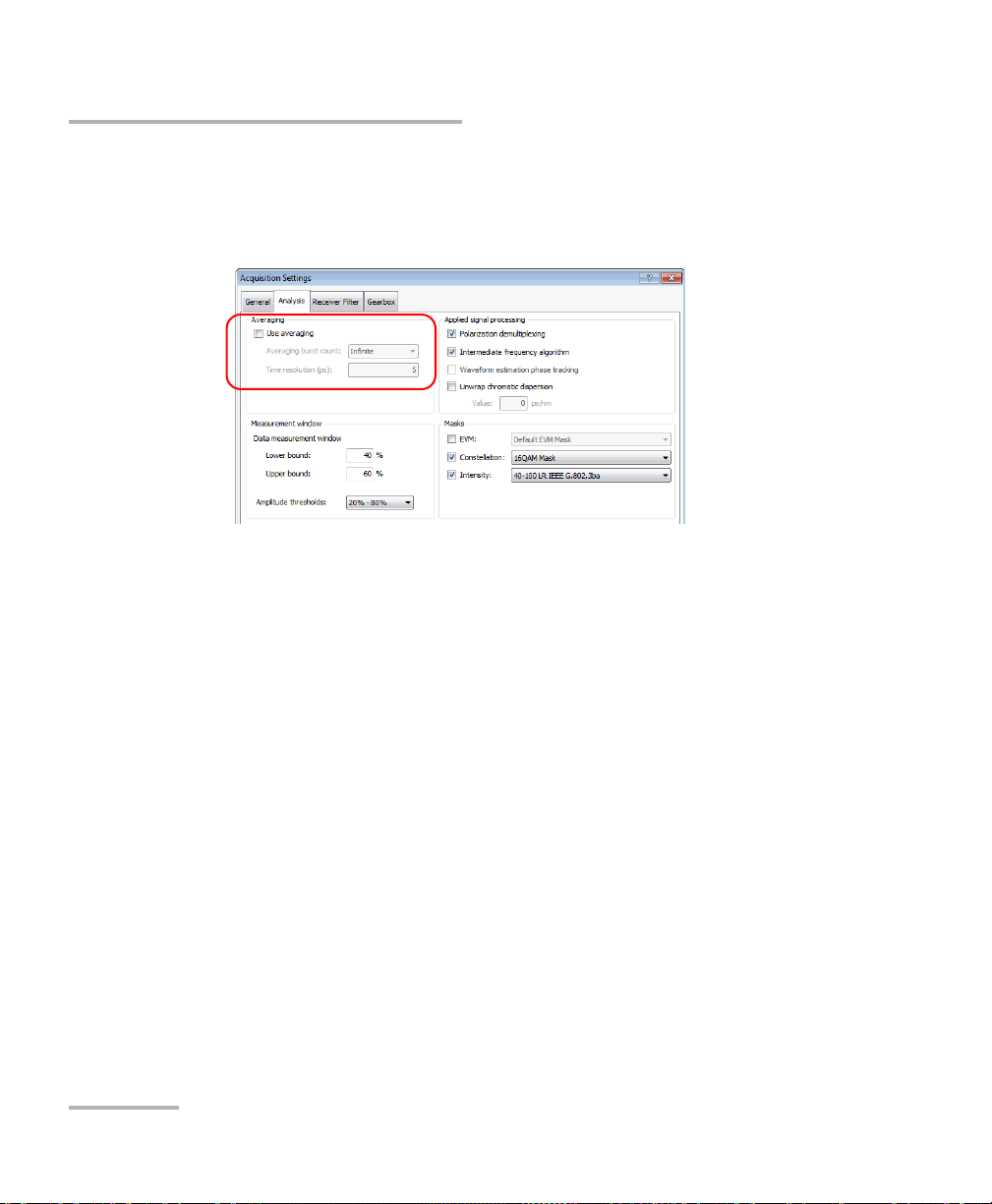
Viewing and Analyzing Results

Applying Advanced Signal Processing Algorithms

To activate and configure averaging:

1. From the Settings menu, select Acquisition.

2. Under the Analysis tab, set the averaging parameters.

 Select Use averaging to activate it (not selected by default).

 Select the number of bursts to average on (1 to 64, or Infinite).

 Set the averaging window (1 to 10 ps, default = 1 ps).

3. Click Apply to confirm your settings, or OK to also close the window.

Applying Advanced Signal Processing Algorithms

You can activate or deactivate specific signal processing algorithms before or while acquiring data, or afterwards in reanalysis mode (see Reanalyzing Acquisitions with New Settings on page 115). The following algorithms are available, depending on the selected modulation format and input pattern:

 Polarization Demultiplexing

For detai l s, s ee Polarization Demultiplexing on page 245.

 Intermediate Frequency Recovery

For detai l s, s ee Intermediate Frequency (IF) Recovery on page 246.

72 PSO-200

Viewing and Analyzing Results

No Phase Tracking

Using Phase Tracking

Applying Advanced Signal Processing Algorithms

 Waveform Estimation Phase Tracking

Increases the PSO-200 phase tracking ability in presence of a large amount of signal phase noise (>1-2 MHz for QPSK). Use when constellation transitions (green samples) suffer from large phase noise whereas symbol center points (white samples) do not spread in phase direction. It utilizes information from the previously acquired waveform to improve the phase tracking of signal transitions.

Note: This algorithm slows down the overall performance.

Optical Modulation Analyzer 73

Viewing and Analyzing Results

No CD Unwrapping

(after 20 bursts)

Using CD Unwrapping

(after 20 bursts)

Applying Advanced Signal Processing Algorithms

 Chromatic Dispersion Unwrapping

Compensates for chromatic dispersion in the signal. You must provide a value (in ps/nm) for use by the algorithm.

Also activates averaging (with the time resolution set based on the signal’s symbol rate). If you deactivate averaging, this algorithm is also deactivated.

74 PSO-200

Viewing and Analyzing Results

Applying Advanced Signal Processing Algorithms

The following table shows algorithms available for each input pattern type:

Algorithm Random

Repetitive

(Unknown)

Known

Patterns

Polarization demultiplexing Yes Yes Yes

IF r ecov e r y Yes Yes Yes

CD unwrapping

No Yes Yes

(as Averaging and Filters)

Waveform estimation

No No Yes

phase tracking

To activate signal processing algorithms:

1. From the Settings menu, select Acquisition.

2. Under the General tab, select one of the values in the Input Pattern

Typ e list. Then provide the necessary pattern details.

3. Under the Analysis tab, select the desired algorithm(s).

4. Click Apply to confirm your settings, or OK to also close the window.

Optical Modulation Analyzer 75

Viewing and Analyzing Results

No Filtering

Using Filtering

(Chebyshev)

Using Filtering

(Bessel)

Applying Data Filtering

The Optical Modulation Analyzer application allows you to apply the following filters to your acquisition:

 Chebyshev (type I only)

 Bessel

 Butterworth

76 PSO-200

Viewing and Analyzing Results

Using Filtering

(Butterworth)

Applying Data Filtering

When you select filtering, the application also activates Average mode (the averaging time resolution will be set based on the signal’s symbol rate). If you deactivate average mode, filtering is also deactivated.

Note: Filters are not available in Random input pattern. They require a pattern

(known or unknown) to function properly.

Note: Filters will not work well with OOK modulation.

To activate and configure a filter:

1. From the Settings menu, select Acquisition.

2. Under the Receiver Filter tab, select Apply filtering to data.

3. Select the desired filter algorithm and parameters.

 Cut frequency (default = signal’s symbol rate)

 Order of the filter (from 1 to 5, default=3)

4. Click Apply to confirm your settings, or OK to also close the window.

Optical Modulation Analyzer 77

8 Bit Pattern Analysis and the

Select Modulation

Select Input Pattern Mode

Repetitive (Unknown)

User-Defined Symbol Pattern

Standard PRBS

User-Defined Bit Pattern

Import symbol pattern and get SER information

Define Gearbox streaming alignment

Can also import bit pattern

Edit/import in application (MAPPING section only)

Can export symbol pattern

Define modulator input mapping and pattern details Can obtain BER information

(Gearbox configuration file)

Edit in Notepad (MAPPING and SYMBOL sections)

Gearbox

The following diagram illustrates the main steps and possibilities in bit pattern analysis using the PSO-200 Optical Modulation Analyzer. With compatible pattern modes, the powerful Gearbox tool allows you to define precisely how your data stream is sent to the modulator and to obtain detailed error rates.

Optical Modulation Analyzer 79

Bit Pattern Analysis and the Gearbox

Basic Gearbox Setup Details

Here are the basic instructions to set the Gearbox for testing. The details for each type of setting is explained further in later sections of this chapter.

To set the Gearbox:

1. From the main window, select the Settings menu, then Acquisition.

2. Under the General tab, select the input pattern type.

Note: The Gearbox can only be used with known patterns, such as PRBS, or a

user-defined pattern.

80 PSO-200

3. Select the Gearbox tab.

4. Select the Gearbox layout.

Bit Pattern Analysis and the Gearbox

Basic Gearbox Setup Details

5. Select the pattern length.

Optical Modulation Analyzer 81

Bit Pattern Analysis and the Gearbox

Basic Gearbox Setup Details

6. Enter the offsets for the bit patterns and indicate whether they are inverted or not. In the case of user-defined patterns, enter the bit stream as well.

To set the bit orders and delays:

1. From the main window, select the Settings menu, then Gearbox

Stream Alignment.

2. In the window, modify the alignments and delays as needed. You can only modify them if you have selected a global or dual X-Y stream.

82 PSO-200

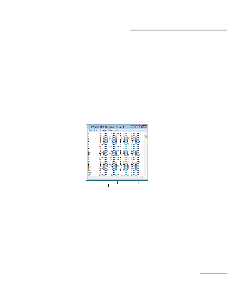
Bit Pattern Analysis and the Gearbox

One line per symbol

I an Q values

for polarization X

I an Q values for polarization Y (if applicable)

Line number

Exporting Symbol Patterns

If the signal data has been acquired with a compatible pattern mode (“Repetitive (unknown)”, “PRBS” or “user-defined”), you can export the actual symbol pattern to a file and reuse it for other acquisitions.

Note: Exporting the symbol pattern from an acquisition in Repetitive mode is

especially useful, since you can reimporting it to obtain better calculations and a symbol error rate. See Importing User-Defined Symbol Patterns on page 84.

The exported file (.osp) is in tab-delimited text format. Here is an example of an exported dual-polarization QPSK symbol pattern, opened in Notepad:

To export a symbol pattern:

1. Select the desired burst (using Playback) from an acquisition made

with a compatible input pattern mode.

2. From the File menu, select Export, then Symbol Pattern.

3. Indicate the location where you want to save the file.

Optical Modulation Analyzer 83

Bit Pattern Analysis and the Gearbox

Importing User-Defined Symbol Patterns

You can import a known symbol pattern from a file and work directly with the symbols in the constellation without having to know the Gearbox details. This allows you to simulate a modulation scheme implementation that is not supported by the PSO-200 or simply to read back symbols information from a previous export.

In this mode, the IF recovery algorithm takes advantage of the known pattern information, and is therefore more robust towards limitations in the signal laser linewidth (phase noise).

The symbol error rate (SER) can be evaluated, but not the bit error rate (BER), since there is no defined mapping between symbols and bits.

The symbol pattern file must have data for the same polarization(s) as the input signal:

 If the signal contains X and Y polarizations and the imported symbol

pattern contains only one, the application will automatically duplicate these values for the Y polarization.

 If the signal contains one polarization and the imported symbol pattern

contains both, the application will truncate the Y data from the pattern.

Note: When importing a symbol pattern, the application will normalize any

non-normalized value.

Note: The Gearbox is not available in this mode.

84 PSO-200

Bit Pattern Analysis and the Gearbox

Importing User-Defined Symbol Patterns

To import a symbol pattern:

1. From the Settings menu, select Acquisition.

2. Select the General tab.

3. In the Input pattern section, select User-defined symbol pattern.

Optical Modulation Analyzer 85

Bit Pattern Analysis and the Gearbox

Length of imported pattern (can then be decreased)

Y polarization data appears if present in the imported file

Importing User-Defined Symbol Patterns

4. Click Import, then select the symbol pattern file (.osp) you want to import and click Open.

5. If needed, enter a smaller value in the Symbol pattern length box. The imported symbol pattern will be truncated when you close the window. The pattern will be unusable if the specified length is larger.

6. Click Apply to confirm your settings, or OK to also close the window.

86 PSO-200

Bit Pattern Analysis and the Gearbox

Performing Detailed Bit Pattern Analysis with the Gearbox

To obtain information such as the probability of error for each individual bit/byte in a pattern, it is essential to get detailed bit pattern analysis capabilities. The PSO-200 Optical Modulation Analyzer can accurately recover the time-domain information without any signal processing due to the high bandwidth achieved with optical sampling. A detailed analysis of the bit pattern recovered can provide a bit error rate (BER) per polarization or map the error vector magnitude (EVM) per symbol. To achieve this, the PSO-200 must receive information on the pattern and sequences used in the transmitter.

For example, consider the following bytes to transmit: D8 A5 69 FE. We need to go further down to the bits since the transmitter is bit-based:

D8 A5 69 FE

1101 1000 1010 0101 0110 1001 1111 1110

We sequence those bits in time by considering the first one to be transmitted as the farthest one on the left (which is the higher rank bit in binary convention).

A bit-pattern generator usually sends bits the way we read them, from left to right. Some may send the bits in reverse order (“0001 1011”), hoping that the receiver will rebuild the sequence correctly.

No matter how the generator sends bits, the Optical Modulation Analyzer application needs a way to determine which bit goes to which modulator input of the transmitter, and which symbol in the constellation represents the recomposed bit pattern. This is where the Gearbox is required.

Optical Modulation Analyzer 87

Bit Pattern Analysis and the Gearbox

Performing Detailed Bit Pattern Analysis with the Gearbox

Gearbox Streaming Types

Depending on how the bit pattern is sent to your transmitter, the Gearbox can be configured as follows:

 One global stream – a single known encoded data stream is

demultiplexed inside the transmitter into several parallel sub-streams sent to the modulator, with delays and inversions (if any).

 N individual streams – as many encoded data streams as there are bits

per symbol (four in the example diagram) are sent with known delays and inversions, if any, to the same number of modulators.

 Dual X-Y streams (dual-polarization modulations only) – two known

encoded data streams corresponding to the X and Y states of polarization are demultiplexed inside the transmitter into parallel streams sent to the modulators.

Note: If the transmitter has an internal encoder, it is the encoded data that must

be input to the Gearbox.

88 PSO-200

Bit Pattern Analysis and the Gearbox

Performing Detailed Bit Pattern Analysis with the Gearbox

There are several ways to implement a data modulator for a modulation format; with these basic Gearbox settings, you should be able to select a combination that suits your data generation. The table below shows all possible configurations for the supported modulations formats.

Modulation Single Polarization Dual Polarization

OOK

1 global stream 1 global stream

BPSK

Dual (X-Y) streams

QPSK 1 global stream 1 global stream

Dual (X-Y) streams

2 individual streams 4 individual streams

Optical Modulation Analyzer 89

Bit Pattern Analysis and the Gearbox

Performing Detailed Bit Pattern Analysis with the Gearbox

Modulation Single Polarization Dual Polarization

APSK 1 Global stream 1 Global stream

3 Individual streams 6 individual streams

Dual (X-Y) streams

90 PSO-200

Bit Pattern Analysis and the Gearbox

Performing Detailed Bit Pattern Analysis with the Gearbox

Modulation Single Polarization Dual Polarization

16-QAM 1 global stream 1 global stream

Dual (X-Y) streams

4 individual streams 8 individual streams

Optical Modulation Analyzer 91

Bit Pattern Analysis and the Gearbox

Performing Detailed Bit Pattern Analysis with the Gearbox

Gearbox Configuration File Layout

A Gearbox configuration file is used by the Optical Modulation Analyzer application to properly map the bit pattern provided as the input to the system.This file is divided into three sections:

 Definition

 Bit symbol mapping and delay

 Symbol coordinates

The file is based on Microsoft’s information file format (.inf). Sections are represented by an uppercase word enclosed in square brackets. Names should not be modified. Values are represented by a name, followed by “=” and the values. Multiple values are separated by a tab (ASCII 09).

The application provides predefined configuration files for all supported modulation schemes. These files are located in the following folder:

\My Documents\EXFO\PSO-200\GearboxSetups

You can edit the files using any text editor. The Mapping section of the file can also be modified from the Optical Modulation Analyzer application.

92 PSO-200

EXFO PSO-200 User Manual

Specifications and Main Features

Frequently Asked Questions

User Manual

Certification Information

European Community Declaration of Conformity

Main Features

Conventions

2 Safety Information

Laser Safety Information

Electrical Safety Information

Installing the EXFO Universal Interface (EUI)

Cleaning and Connecting Optical Fibers

Starting and Exiting the Optical Modulation Analyzer Application

Configuring the Input Signal

Setting Other Acquisition Parameters

Setting File Autonaming

Identifying Acquisitions

Setting Analysis Parameters

Using Special Modulation Modes

Using an External Local Oscillator

Locking the Remote Unit

5 Performing Acquisitions

Starting and Stopping an Acquisition

Clearing Data During an Acquisition

Saving Acquisitions to a File

Activating Trigger-Based Acquisitions

Selecting and Customizing the Layout

Constellation Chart

Eye Diagrams

Pattern Diagrams

Y-Axis Auto Scaling (All Graphs)

Opening an Existing Acquisition File

Viewing Acquisition Information

Playing Back Acquisition Files

Zooming and Moving Graphs

Displaying and Setting X-Axis Values

Displaying Graphs in Color Grade Mode

Displaying Multiple Bursts Simultaneously (Persistence)

Setting Number of Symbol Periods for Eye Diagrams

Using the Measurement Tables

Using Graph Markers

Viewing Signal Distribution Using Histograms

Distinguishing Data Points from Transitions

Using Pattern Masks

Using Averaging to Improve Results

Applying Advanced Signal Processing Algorithms

Applying Data Filtering

Basic Gearbox Setup Details

Exporting Symbol Patterns

Importing User-Defined Symbol Patterns

Performing Detailed Bit Pattern Analysis with the Gearbox