ESA Environment Programming Description

OEM Environment

Programming Description (DP)
User Documentation

Valid for:
Product: Kvara SW 162

from version 3.14

Edition: June 2003
Code: 91752.DP.1.GB

Esa/Gv s.r.l.
15 via Zamboni, Cp 43
41011 Campogalliano Modena Italy
tel. [phone] - fax [phone]
http://www.esagv.it - E-mail: [email protected]

Restrictions

Duplication, transmission and use of this document or its contents shall be considered
prohitibed unless prior authorization has been received from Esa/Gv. All rights are
reserved.
Even when authorized, modification of this document (either by computer or on paper)
voids the guarantees specified below.

Guarantees

Editions

Notes

The product may offer performances that are not described in these manuals. Esa/Gv
shall neither be obliged to maintain these functions in new versions of the product nor
to guarantee the relative assistance.

Checks have been carried out in order to ensure that the contents of these manuals
correspond to the documented product. Despite this fact, there may be discrepancies.
Esa/Gv therefore offers no guarantees as to the full compliance and completeness of the
texts.
The information in this document is periodically revised and new editions are issued
when necessary.

This manual has been compiled in partial compliance with ANSI/IEEE std 1063-1987
“IEEE Standard for software User Documentation”.

This document is liable to be modified without prior notice. These modifications may
involve further editions or revisions of the document.
Further editions imply complete substitution of the document.
Revision involves replacement/addition/elimination of pages of the document.
Each page is identified by the code of the document at the bottom.

MS-DOS® Trademark registered by Microsoft Corporation.

91752.DP.1.GB Esa/Gvii

The chronological list of editions of this document is given in the following table:

Evolution of the document

Edition Document Code Release Type of edition

19/03/2001 91752.DP.0.GB 0 New document
04/06/2003 91752.DP.1.GB 1 Revision

Modifications

Release Chapters - Pages Description

Esa/Gv 91752.DP.1.GB iii

91752.DP.1.GB Esa/Gviv

DP Programming Description

Programming Description

Notes for the reader....................................................................................................... i

Explanation of the symbols..................................................................................................................ii

Printer’s conventions..........................................................................................................................iii

Glossary .............................................................................................................................................iv

1 Introduction............................................................................................................. 1.1

1.1 Definitions...................................................................................................................................1.1

1.2 Conventions used in the description of the syntax.....................................................................1.4

2 Standard Programming.......................................................................................... 2.1

2.1 Writing a program.......................................................................................................................2.1

2.1.1 An C program................................................................................................................2.1

2.1.2 Program start ................................................................................................................2.1

2.1.3 Selecting ISO mode......................................................................................................2.2

2.1.4 Program end .................................................................................................................2.2

2.1.5 Block number................................................................................................................2.3

2.1.6 Messages......................................................................................................................2.3

2.2 Setting machining conditions......................................................................................................2.4

2.2.1 Defining a point .............................................................................................................2.4

2.2.2 Interpolation parameters...............................................................................................2.4

2.2.3 Absolute point programming.........................................................................................2.5

2.2.4 Incremental programming.............................................................................................2.6

2.2.5 Selecting the unit of measurement................................................................................2.6

2.2.6 Selecting origin translation............................................................................................2.7

2.2.7 Cancelling origin translation..........................................................................................2.8

2.2.8 Additive origin translation..............................................................................................2.9

2.2.9 Selecting the work plane...............................................................................................2.9

2.2.10 Selecting the contour milling plane and the length correction direction....................2.11

2.3 Programming the feed..............................................................................................................2.12

2.3.1 Feed command...........................................................................................................2.12

2.3.2 Rapid feed...................................................................................................................2.13

2.3.3 Linear interpolation......................................................................................................2.14

2.3.4 Circular interpolation ...................................................................................................2.15

2.3.5 Thread-cutting.............................................................................................................2.16

2.3.6 Tapping .......................................................................................................................2.18

Esa/Gv 91752.DP.1.GB i

Programming Description DP

2.3.7 Timed halt ...................................................................................................................2.19

2.3.8 Positioned halt.............................................................................................................2.19

2.4 Special interpolations ...............................................................................................................2.20

2.4.1 Auxiliary axis interpolations.........................................................................................2.20

2.4.2 Cylindrical programming .............................................................................................2.20

2.5 Spindle orientation....................................................................................................................2.22

2.5.1 M19: Spindle orientation..............................................................................................2.22

2.5.2 On-the-fly spindle orientation ......................................................................................2.23

2.6 Programming axis and spindle speed......................................................................................2.24

2.6.1 Setting the feed rate....................................................................................................2.24

2.6.2 Continuous feed mode................................................................................................2.25

2.6.3 Continuous feed mode with speed look-ahead...........................................................2.26

2.6.4 Selecting the feed mode .............................................................................................2.27

2.6.5 Selecting the spindle rotation mode............................................................................2.28

2.6.6 Setting the spindle rotation mode................................................................................2.28

2.6.7 Inverse feed ................................................................................................................2.31

2.7 Polar axes programming..........................................................................................................2.33

2.7.1 Polar axes with travel limitation...................................................................................2.33

2.7.2 Round axes.................................................................................................................2.33

2.7.3 Selection of the direction and rpm rate .......................................................................2.35

2.7.4 Speed programming in the presence of polar axes....................................................2.39

2.8 Auxiliary Functions....................................................................................................................2.41

2.8.1 Functions M and T ......................................................................................................2.41

2.9 Tool compensation...................................................................................................................2.43

2.9.1 Tool length correction..................................................................................................2.43

2.9.2 Tool radius compensation...........................................................................................2.44

3 Advanced Programming......................................................................................... 3.1

3.1 Selecting Automation Language mode.......................................................................................3.1

3.2 Parametric Programming ...........................................................................................................3.2

3.2.1 Global system variables................................................................................................3.2

3.2.2 Pre-defined numeric variables ......................................................................................3.3

3.2.3 Assigning a variable pre-defined numeric variables......................................................3.3

3.2.4 Symbolic variables ........................................................................................................3.4

3.2.5 Declaration of Symbolic Variables.................................................................................3.4

3.2.6 Allocation of Symbolic Variables...................................................................................3.6

3.2.7 Expressions...................................................................................................................3.7

91752.DP.1.GB Esa/Gvii

DP Programming Description

3.2.8 Use of #QNAN ............................................................................................................3.15

3.3 Program flow control.................................................................................................................3.16

3.3.1 Unconditional jump......................................................................................................3.16

3.3.2 Test.............................................................................................................................3.16

3.3.3 Conditioned Test.........................................................................................................3.17

3.3.4 WHILE Block...............................................................................................................3.18

3.3.5 REPEAT Block............................................................................................................3.19

3.3.6 FOR Block...................................................................................................................3.20

3.3.7 Cycle interruption - BREAK.........................................................................................3.21

3.3.8 Repeat.........................................................................................................................3.22

3.3.9 Nesting levels: sub-programs and fixed cycles...........................................................3.23

3.3.10 Subprogram start (fixed cycle)..................................................................................3.24

3.3.11 Subprogram end (fixed cycle)...................................................................................3.25

3.3.12 Program end .............................................................................................................3.26

3.3.13 Call to subprogram CFU (user fixed cycle)...............................................................3.26

3.3.14 Subprogram call CFS (system fixed cycle)...............................................................3.27

3.3.15 Cancels a fixed cycle's mode....................................................................................3.28

3.3.16 Call-back function in “C” language............................................................................3.29

3.3.17 Forced escape from the interpreter with error...........................................................3.30

3.4 Special functions ......................................................................................................................3.31

3.4.1 Await termination.........................................................................................................3.31

3.4.2 Message display in phase with the executor...............................................................3.31

3.4.3 Memory read/write.......................................................................................................3.31

3.4.4 Enter a physical or logical output ................................................................................3.32

3.4.5 Enabling hydraulic tapping ..........................................................................................3.33

3.4.6 Defining path axes ......................................................................................................3.34

3.4.7 Definition of the Axes belonging to the Channel .........................................................3.35

3.4.8 Correction by zones ....................................................................................................3.36

3.4.9 Enabling program simulation.......................................................................................3.37

3.4.10 Identifier of the number of the channel being executed............................................3.38

3.4.11 Probe target reading..................................................................................................3.39

3.4.12 Axis target reading ....................................................................................................3.39

3.5 Reference system transformations...........................................................................................3.41

3.5.1 PRS - Preset machine origin.......................................................................................3.41

3.5.2 DEF - Run-time redefinition of the axis names...........................................................3.41

3.5.3 SYS – Run-time re-allocation of the axes name.........................................................3.42

3.5.4 MIR - Mirrored machining............................................................................................3.42

Esa/Gv 91752.DP.1.GB iii

Programming Description DP

3.5.5 ROT – Rotation of the contouring plane......................................................................3.45

3.5.6 SHF – Transfer of Origin.............................................................................................3.46

3.5.7 MLV - Selection of the matric conversion level...........................................................3.47

3.5.8 Definition of a tilting plane...........................................................................................3.49

3.5.9 Tilting plane enabling ..................................................................................................3.50

3.6 Automatic plane geometry........................................................................................................3.51

3.6.1 Chamfer between two linear segments.......................................................................3.51

3.6.2 Radius between two linear segments .........................................................................3.52

3.7 Tool corrector auxiliary functions..............................................................................................3.53

3.7.1 Machining allowance management.............................................................................3.53

3.7.2 Tangential feed in/out..................................................................................................3.53

3.7.3 Tool life and wear management..................................................................................3.55

3.8 Three dimensional tool corrector..............................................................................................3.56

3.8.1 TWI: Spindle settings..................................................................................................3.56

3.8.2 THD: Tool holder settings ...........................................................................................3.56

3.8.3 Conventions regarding angles of rotation ...................................................................3.56

3.8.4 Orientation with polar axis coordinates .......................................................................3.57

3.8.5 Orientation by Euler's Angles......................................................................................3.57

3.8.6 Orientation by roll-pitch-yaw (RPY).............................................................................3.59

3.8.7 Orientation by the tool axis unit vector........................................................................3.60

3.8.8 Vectorial tool radius compensation.............................................................................3.62

3.8.9 Automatic determination of the pertinent plane and machining with the axis in tangency

...................................................................................................................................3.63

3.8.10 Discriminating between the interchangeable cutting edges of a tool........................3.67

3.8.11 Machining depth compensation along the tool axis ..................................................3.69

3.8.12 Machining depth compensation along the tool radius...............................................3.70

3.9 Feed in strategies.....................................................................................................................3.71

3.9.1 Definitions....................................................................................................................3.71

3.9.2 Axial/radial feed in.......................................................................................................3.71

3.9.3 Axial/radial feed out.....................................................................................................3.74

3.9.4 Compensation depending on a section of the tool along the trajectory in its in-going

point ...........................................................................................................................3.78

3.9.5 Compensation depending on a section of the tool along the trajectory in its out-going

point ...........................................................................................................................3.82

3.10 Feed Control...........................................................................................................................3.83

3.10.1 Modification or Automatic speed control parameters................................................3.83

3.11 Independent axis synchronous/asynchronous positioning.....................................................3.85

3.11.1 Independent axis synchronous positioning ...............................................................3.85

91752.DP.1.GB Esa/Gviv

DP Programming Description

v

3.11.2 Independent axis asynchronous positioning .............................................................3.86

3.11.3 Prallel spindle orientation..........................................................................................3.87

3.12 Modifying axis parameters......................................................................................................3.88

3.12.1 Following error...........................................................................................................3.88

3.12.2 Axis acceleration time...............................................................................................3.88

3.12.3 Axis deceleration time...............................................................................................3.89

3.12.4 Axis emergency deceleration time............................................................................3.89

3.12.5 Axis maximum speed................................................................................................3.90

3.12.6 Axis ramp to S...........................................................................................................3.91

3.12.7 Axis jerk settings.......................................................................................................3.92

3.13 Modification of the interpolation parameters ..........................................................................3.93

3.13.1 Interpolation acceleration time setting.......................................................................3.93

3.13.2 Interpolation deceleration time setting ......................................................................3.93

3.13.3 Maximum interpolation speed setting........................................................................3.94

3.13.4 Interpolation ‘S’ ramp time setting.............................................................................3.94

3.13.5 Jerk setting during interpolation................................................................................3.95

4 Fixed Cycle Systems (FCS).................................................................................... 4.1

4.1 G192 macro Generation of a grid of points................................................................................4.2

4.2 G193 macro - generation of points distributed along a circumference arc.................................4.5

4.2.1 G81 Fixed Cycle: drilling ...............................................................................................4.7

4.2.2 G83 Fixed Cycle: drilling with swarf discharge or breaking...........................................4.9

4.2.3 G84 Fixed Cycle: Tapping...........................................................................................4.12

4.2.4 G86 Fixed Cycle: Boring .............................................................................................4.13

4.2.5 G88 Fixed Cycle: drilling cavity walls ..........................................................................4.14

4.2.6 G133 Fixed cycle: Thread-cutting...............................................................................4.16

5 Tool parameters...................................................................................................... 5.1

5.1 Definitions...................................................................................................................................5.1

5.2 ER (Entity Relationship) diagram of the entities of a machining center of which the geometry

and power train are controlled....................................................................................................5.3

5.2.1 Key................................................................................................................................5.3

5.2.2 Diagram.........................................................................................................................5.3

5.3 Other definitions .........................................................................................................................5.5

5.4 Head descriptor..........................................................................................................................5.6

5.4.1 Data structure................................................................................................................5.6

5.4.2 Description of the geometry and actuators ...................................................................5.7

5.5 Toolholder descriptor................................................................................................................5.13

Esa/Gv 91752.DP.1.GB

Programming Description DP

5.5.1 Data structure..............................................................................................................5.13

5.5.2 Description of geometry..............................................................................................5.13

5.6 Tool or tool cutter descriptor.....................................................................................................5.15

5.6.1 Data structure..............................................................................................................5.15

5.6.2 Description of geometry..............................................................................................5.15

5.6.3 Description of other technological data.......................................................................5.17

5.6.4 Logic management......................................................................................................5.18

5.6.5 Broken tools ................................................................................................................5.18

END OF SUMMARY

91752.DP.1.GB Esa/Gvvi

DP Notes for the reader

Notes for the reader

General information

Purpose

Users

Use of the document

Notification of
difficulties

The information in this manual only applies to the software versions indicated on the
frontispiece.

Not all the available functions may be described in this manual. In these cases, Esa/Gv
shall be obliged to neither guarantee these functions nor include them in future versions.

The purpose of this document is to help the operator when programming the processes.

This document contains information for:
ù technicians with a good working knowledge of the processing technology and

productive process. Basic knowledge of computer work.

The document is divided into chapters that describe the programming operations, the
language and basic processing concepts.

Please contact Esa/Gv if any difficulties should arise when this manual is used.

Esa/Gv 91752.DP.1.GB i

Notes for the reader DP

Explanation of the symbols

Graphic symbols may appear beside the text. These are used to emphasize information
of particular importance.

Attention
This symbol is used when failure to take the appropriate precautions could cause slight
damage to persons and property.

Danger

This symbol appears when failure to take the appropriate precautions or
accomplishment of incorrect manoeuvres could cause serious damage to persons

and/or property.

Important

This symbol appears in the manual to indicate information of particular importance. It
is essential to read these sections in order to fully understand the manual.

Option

This symbol indicates sections of the manual that describe optional functions or parts.
Use of optional performances must be established with the machine manufacturer.

Manufacturer

This symbol indicates those sections of the manual reserved to the machine
manufacturer.

Password

This symbol indicates sections of the manual that describe functions access to which is
safeguarded by software passwords.

CN

This symbol indicates sections of the manual that describe functions only available in
CN and not in the PC.

PC

This symbol indicates sections of the manual that describe functions only available in
the PC and not in CN.

91752.DP.1.GB Esa/Gvii

DP Notes for the reader

Printer’s conventions

Particular printer’s conventions are used to make it easier to identify the information in
this manual. These conventions are illustrated below.

Keyboard and video

The following conventions are used.
ù The names of the screen-printed keys are indicated in boldface and are enclosed

within square brackets. If the name of the key is preceded by “button”, reference is
being made to a key on the push button panel.

− [ENTER]. Identifies the key that bears the word ENTER.

− [+] indicates the + key of the keyboard, while button [+] indicates the + key of

the push button panel.

ù The names of the function keys are indicated in boldface italics and are enclosed

within square brackets.

− [Plc Menu]. Identifies the function key that bears the words Plc Menu.

ù References to fields and/or messages on the video are written in boldface italics.
ù The specific text to be digitized by the user is underlined.

− If the manual indicates “digitize ok, the user must digitize exactly “ok”.

ù DIRECTION or DIRECTIONAL keys is the collective name used to indicate the

UP, DOWN, LEFT and RIGHT keys.

ù Pressure, in sequence, on a series of keys is written by separating the identifiers of

the required keys with the “>“ character.

− [Manual] > [START]. Describes pressure, in sequence, on the [Manual] and

[START] keys.

Text

ù Pressure on several keys at the same time is indicated by separating the identifiers of

the keys themselves with the “+” character.

− [SHIFT] + [àà] Describes contemporaneous pressure on the [SHIFT] and [àà]

keys.

The following conventions are used.

ù Italics are used to identify specialistic terms.
ù Boldface is used to emphasize words of particular importance.

Esa/Gv 91752.DP.1.GB iii

Notes for the reader DP

Glossary

CNC

This is an abbreviation of Computerized Numerical Control and indicates the instrument
that governs the machine, i.e. the electronic device through which the machining cycles
are programmed, the axes moved, etc..
It corresponds to one of the devices whose operation is described in this manual.

END OF PREFACE

91752.DP.1.GB Esa/Gviv

DP Introduction

1 Introduction

This chapter describes certain fundamental concepts that are at the basis of CNC
programming.
Examples containing instructions in the programming language will be used to highlight
certain aspects, while the explanation of each instruction is given in the dedicated
chapter.

1.1 Definitions

Program

Block

Word

A program is a sequence of blocks, or program lines, that specify the various machining
phases.

A block consists of one or more words and terminates with the line feed character
([RETURN] key)

A word consists of a literal code and a number, not separated by spaces.

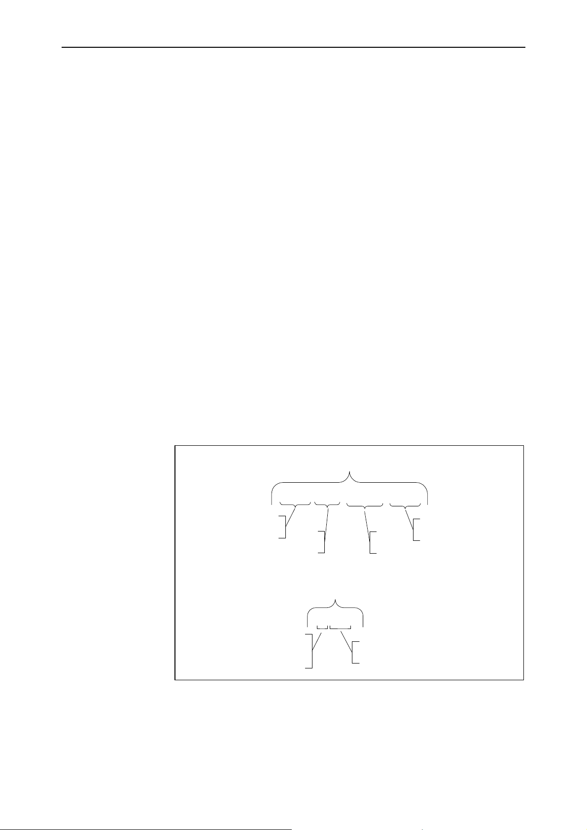
Example of a block formed by three words:

N100 X100.00 Y100.00

Characters N, X and Y identify the type of words in the block.

Example:

Block

G17 G2 X200 R60

Word

Word

Word

Word

Word

X200

Word

Type

Figure 1.1 - Composition of a Block and a Word

Esa/Gv 91752.DP.1.GB 1.1

Field

Introduction DP

Do not attempt to execute the sequence of commands in the previous example on the
machine. All the data specified are purely fictitious.

Program execution

Execution flow

Axis

Program execution is the same as executing the blocks that form it in the established
order in order to obtain one or more machining operations.

The execution flow is the sequence with which the instructions in a program or list are
executed. In the more simple cases, execution takes place in sequence starting from the
first instruction and terminating with the last (sequential flow). In other cases, the flow
can be altered, repeating or conditioning the execution of certain instructions (non­sequential flow).

An axis is a mechanical and electronic entity thanks to which the NC can control the
position of an element of the machine in relation to a reference point.

Three axes square to each other are required too identify a point in the three­dimensional space. They are conventionally called X, Y and Z (main axes).
Z axis is generally parallel to the axis of rotation of the spindle.
The following axes can be defined:

X
Y
Z

Main axis
Main axis
Main axis

Origin

U
V
W
A
B
C

The target of an axis always refers to a point (origin) and can be expressed in:

ù Millimeters or inches for linear axes
ù degrees for rotational axes

An origin is a point in space to which the axes targets refer.
After the sizing cycle, which normally takes place whenever the CNC is powered, the
axes are referred to the machine origin. However, when it comes to workpiece
programming, the targets can be referred to the workpiece origin which will be shifted in
relation to the machine origin by a value in the origin parameters, depending on the
position in which the workpiece clamping system is to be found.

Auxiliary axis parallel to X
Auxiliary axis parallel to Y
Auxiliary axis parallel to Z
Rotational axis with axis of rotation parallel to X
Rotational axis with axis of rotation parallel to Y
Rotational axis with axis of rotation parallel to Z

91752.DP.1.GB Esa/Gv1.2

DP Introduction

Modal function

Default function

A programming function (or address) is called modal if its effect also affects the
successive blocks, through to activation of another function that excludes the first.
A non-modal function, that only has effect in the block in which it is programmed, is
also called self-cancelling.

A modal programming function is by default if it is activated automatically at the start of
the program.

Esa/Gv 91752.DP.1.GB 1.3

Introduction DP

1.2 Conventions used in the description of the syntax

Recourse is made to a conventional notation in the description of the syntax of each
instruction:

Capital text, for
example: Y, R,I, J, ...

Target

Angle

Indicates the name of an address within a command.

Indicates a field in which the following information can be entered:
ù A numeric value with sign and decimals used to indicate any coordinate or distance.

When the parameter that indicates the display unit is varied, the measurements will
be automatically converted from millimeters into inches, and vice versa. For inches,
two decimal figures are added as compared to the measurements expressed in
millimeters;

ù A variable (see “Programming concepts”, Parametric Programming” section).

Indicates a field in which the following information can be entered:
ù An angle, expressed in degrees/decimal fractions of a degree (from 0.00 to 359.99).

The sexagesimal system cannot be used. Values of 360 or more or negative values
will be normalized, i.e. they will be brought within the 0 to 359.99 range.

ù A variable.

END OF CHAPTER

91752.DP.1.GB Esa/Gv1.4

DP Standard Programming

2 Standard Programming

2.1 Writing a program

2.1.1 An C program

A NC program or partprogram is a sequence of blocks which define the machining of a
workpiece (part) on a numerical control machine tool.

PROGRAM START

BLOCKNUM WORDS COMMENT
BLOCKNUM WORDS COMMENT
BLOCKNUM WORDS COMMENT

... ...

2.1.2 Program start

Syntax

Description

Example

PROGRAM END

comment %program_number

The program start block must precede all other blocks of the self program.

Comment An alphanumerical character string which briefly

describes the program.
È a comment must be inserted before the character %.

program_number A unique identifying number which corresponds to the

partprogram number.

THREAD 3/8 GAS %1200

....

....

program body

....

....

M30

See also

Esa/Gv 91752.DP.1.GB 2.1

Program end, Subprogram start ( "Advanced programming").

Standard Programming DP

2.1.3 Selecting ISO mode

Syntax

Description

Example

2.1.4 Program end

Syntax

MODE = ISO
MODE = AUTO (default)

Assign the value ISO to the system variable MODE to select writing a partprogram
according to ISO/DIS 6983 (Parts I and II) Draft International Standard, September
1982 (Part I) and July 1988 (Part II).
In this mode Automation Language-specific features are not available.
In ISO mode comments are preceded by round brackets and an asterisk.

(* INSERT WORKING PROGRAM)
N5 G17 (* WORK PLANE X-Y)
N15 G0 B90 (* TURN CNC TABLE 90 DEGREES)
N20 T1 M6 (*RECALLS TOOL/SPINDLE )
(*TOOL DIAMETER 10 )
N30 D1 (*TOOL CORRECTOR)
N40 G0 X0 Y0
N50 Z125

M2 or M30

Description

Example

See also

The program end block stops execution of the program.

THREAD 3/8 GAS %1200

....

....

program body

....

....

M30

Program start.

91752.DP.1.GB Esa/Gv2.2

DP Standard Programming

2.1.5 Block number

Syntax

Description

Example

2.1.6 Messages

Syntax

Nblock_number

The block number is an optional word which must precede the other words in the block.
It gives a unique reference to the block itself.

block_number Unique block reference number.

COMMENT %1
N10 X100 Y100 (feed to point P1(X100,Y100))
N20 Y200 (feed to point P2(X100,Y200))
G04 F1

....

....

M30

(text)

Description

Example

In ISO programming mode, text in round brackets () is displayed as

text A sequence of alphanumerical characters.

N100 (ERROR: PRESS RESET)
N110 G04 F1
N120 JMP 110 (loop while awaiting reset)

Esa/Gv 91752.DP.1.GB 2.3

Standard Programming DP

2.2 Setting machining conditions

2.2.1 Defining a point

Syntax

Description

Xpos Ypos Zpos Upos Vpos Wpos Apos Apos Bpos Cpos

An axis code followed by a number defines a point's position on the axis.
To define a point the words for all the defined axes must be contained in a single block.
If a word relative to a given axis is missing, the system sets that axis to its value in the
definition of the preceding point.

Xpos
Ypos
Zpos
Upos
Vpos
Wpos
Apos
Bpos
Cpos

Example

X100 Y100 (feed to point P1(X100,Y100))
Y200 (feed to point P2(X100,Y200))

See also

Feed command.

2.2.2 Interpolation parameters

Syntax

Description

Ipos (value on the X axis)
Jpos (value on the Y axis)
Kpos (value on the Z axis)
Rpos (radius of a circle)

Interpolation parameters define the basis for interpolation.
The codes I, J and K are used to define the coordinates of the centre of a circular
interpolation and the pitch in thread-cutting and tapping.
The code R defines the radius of a circular interpolation arc.

91752.DP.1.GB Esa/Gv2.4

DP Standard Programming

Ipos
Jpos
Kpos
Rpos

Example

See also

See the examples under Circular interpolation, Thread cutting,Tapping.

Circular interpolation, Thread cutting,Tapping

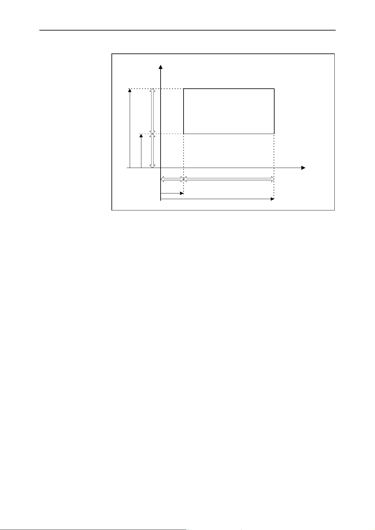
2.2.3 Absolute point programming

Syntax

Type of function

Description

Example

G90

Modal, default, mutually exclusive with G91

Absolute programming defines the points relative to the axis origins as defined at the
time.

G90 X200 Y300 (feed to point P1(X200,Y300)
Y700 (feed to point P2(X200,Y700)
X1000 (feed to point P3(X1000,Y700)
Y300 (feed to point P4(X1000,Y300)
X200 (feed to point P4(X200,Y300)

See also

Esa/Gv 91752.DP.1.GB 2.5

Defining a point,Incremental programming.

Standard Programming DP

y

G91

G90

G90

G91

Figure 2.1 - Incremental and absolute programming

2.2.4 Incremental programming

Syntax

Type of function

Description

Example

G91

Modal, mutually exclusive with G90

Incremental programming defines the points relative to the latest preceding point.
The I, J and K positions are also relative to the preceding values of the X, Y and Z axes.

X100 Y100 feed to point P1(X200,Y300)
G91 Y100 feed to point P2(X100,Y200)
X100 feed to point P3(X200,Y200)
Y-100 feed to point P4(X200,Y100)

G91
G90

G90

G91

x

See also

Defining a point,Absolute point programming.

2.2.5 Selecting the unit of measurement

Syntax

G70 (dimension in inches)
G71 (dimension in mm)

91752.DP.1.GB Esa/Gv2.6

DP Standard Programming

Type of function

Description

Example

See also

Modal, default, settable by a machine parameter

Selects programming in imperial or metric dimensions.
All axes are thus measured in inches (values after axis codes) except for the rotary axes
(A,B,C), the dimensions which define the centre of a circle, and the radius dimension.

X100 Y100 (feed to point P1(X100,Y100))
G70 G91 Y3 (feed to point P2(X100,Y100+3*25.4))

Defining a point.

Esa/Gv 91752.DP.1.GB 2.7

Standard Programming DP

2.2.6 Selecting origin translation

Syntax

Type of function

Desription

Example

See also

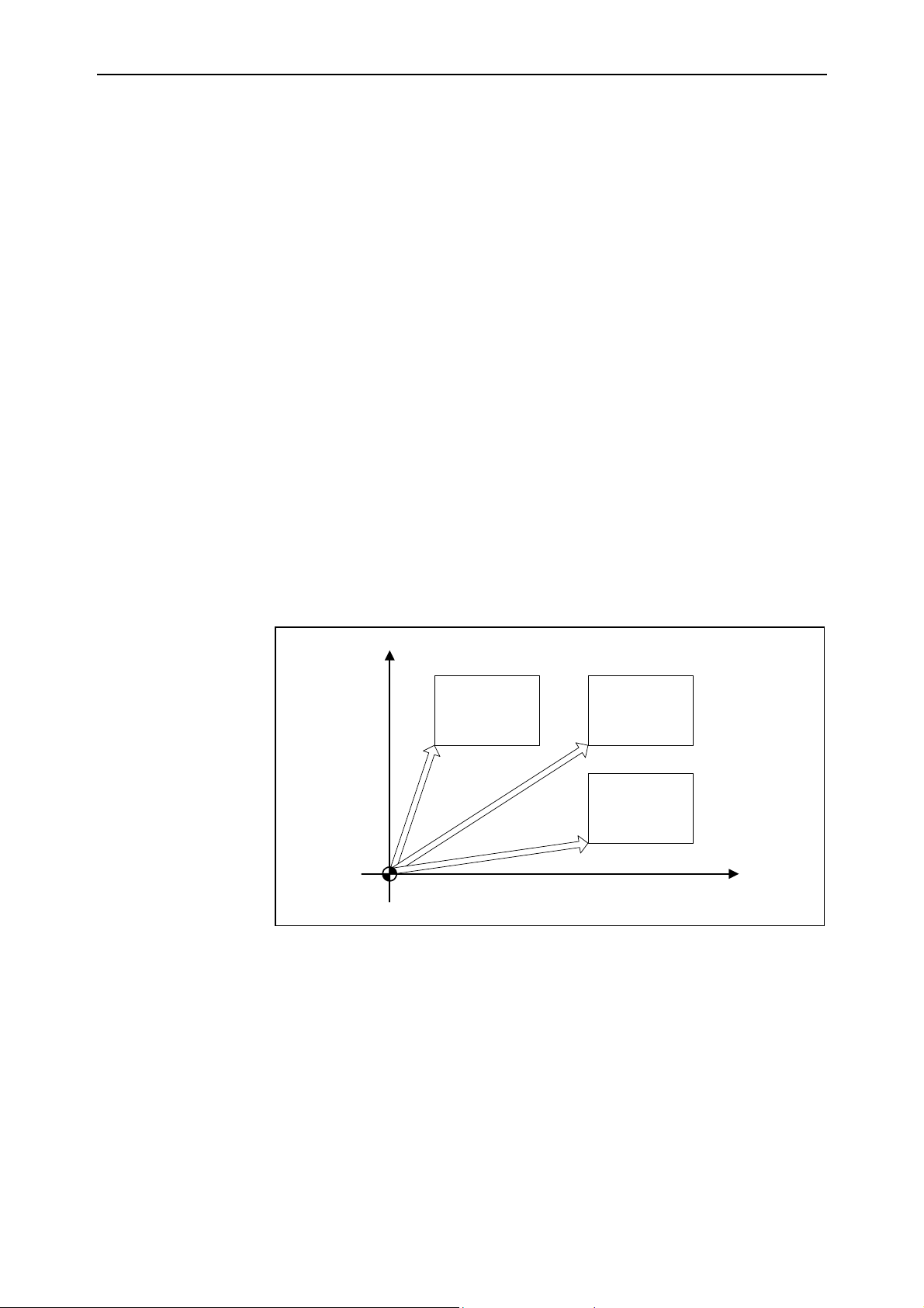
G54 to select translation of origin 1
G55 to select translation of origin 2
G56 to select translation of origin 3
G57 to select translation of origin 4

Modal, mutually exclusive with G53

Origin translation allows selection of one of the four part origins set by the operator via
the user interface. In the blocks after the origin selection block, the positions and tool
movements refer to the currently selected origin.
This function only works in cartesian coordinates XYZ.

X100 Y100 (feed to point P1(X100,Y100))
G54 Y200 (feed to point P2(Xinalterato,Y200) relative to
part origin 1)

Defining a point,Cancelling origin translation.

y

G54

Figure 2.2 - Programming the part origins

91752.DP.1.GB Esa/Gv2.8

G55

G56

x

DP Standard Programming

2.2.7 Cancelling origin translation

Syntax

Type of function

Description

Example

See also

G53

Self-cancelling, default, mutually exclusive with G54, G55, G56, G57

Inclusion of this function in a block switches off the "origin translation" and "tool
compensation" functions. The programmed dimensions are therefore referred to the
machine origin.
This function is used for positioning the tool with respect to the machine origin,
irrespective of the part origin (for example, for returning to the tool magazine).

G54 X100 Y100 (feed to point P1(X100,Y100) relative to the
part origin)
G53 X1000 Y2000 (feed to point P2(X1000,Y2000) relative to
the machine origin)
X100 Y200 (feed to point P3(X100,Y200) relative to the
part origin)

Defining a point, Selecting origin translation.

Esa/Gv 91752.DP.1.GB 2.9

Standard Programming DP

2.2.8 Additive origin translation

Syntax

Type of function

Description

Example

G58 Xpos Ypos .....for additive translation of origin 1

G59 Xpos Ypos .....for additive translation of origin 2

Modal

Xpos
Ypos
Zpos

Additive origin translation adds origin translation dimensions to the part origin, for
defining local origins on the part as required.
The translation values are defined for the primary axes (XYZ) or the auxiliary axes
(UVW), by the values set in the same block.
To cancel additive origin translation, set the translation values to zero.

X100 Y100 (feed to point P1(X100,Y100))
G58 Y50 (move the origin to P2(X0, Y50))
X100 Y100 (feed to point P3(Xunchanged,Y+50))
G58 Y0 (reset the part origin)

See also

Defining a point, Selecting origin translation.

2.2.9 Selecting the work plane

Syntax

Type of function

Description

G17 (select XY plane, compensate tool length on Z)
G18 (select ZX plane, compensate tool length on Y)
G19 (select YZ plane, compensate tool length on X)

Modal.
Default: G18 if the Y axis does not exist (lathe), otherwise G17.

Selecting the work plane defines:

ù the plane on which the arc is executed in a circular interpolation
ù the axis along which the tool is compensated
ù the plane for tool radius correction

91752.DP.1.GB Esa/Gv2.10

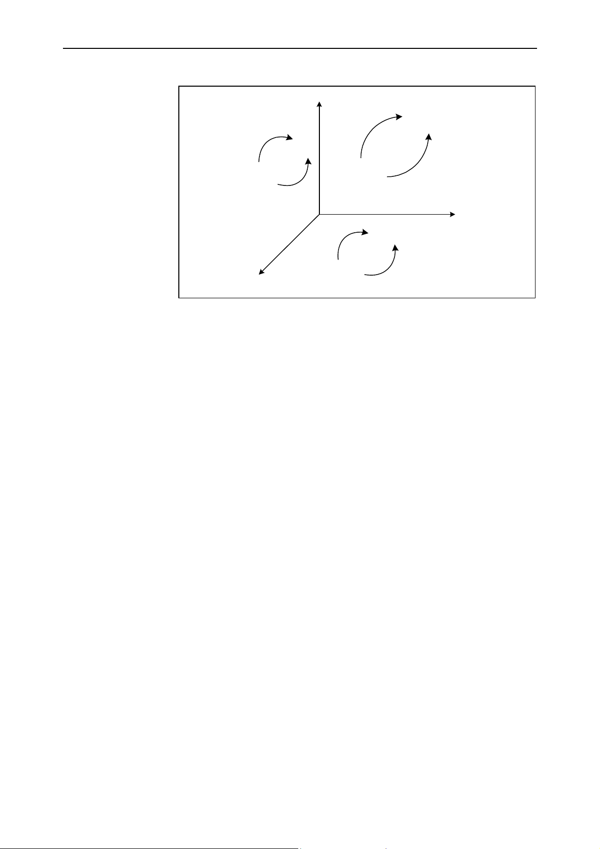
DP Standard Programming

Y

G2

G2

G17

G19

G3

G3

Example

See also

G2

X

G18

Z

Figure 2.3 - Work plane

X100 Y100 (feed to point P1(X100,Y100))
G17 G2 X200 R60 (executes an arc on the XY plane)

Circular interpolation,Tool compensation.

G3

Esa/Gv 91752.DP.1.GB 2.11

Standard Programming DP

2.2.10 Selecting the contour milling plane and the length correction direction

Syntax

Type of function

Description

Example

G16 <name axis I> <name axis II> <name axis III> <direction of length correction>

Modal.

Selects the contour milling plane(or where the tool radius correction is applied) by
selection of the first and second axis. Any contour milling plane can be specified.
Furthermore, G16 enables selection of the direction and axis of length correction via
specification of the third axis and sign ('+' / '-'). The third axis can be freely chosen from
among the configured cartesian axes. Tool correction cannot therefore be applied
directly along an auxiliary (UVW) or polar (ABC) axis.

G16 has the following features:

ù definition of the radius correction plane (which is also the machining plane).
ù definition of the axis and direction of length correction;

G17 àG16 XYZ+
G18à G16 ZXY+
G19à G16 YZX+

G16 U Z Y+

91752.DP.1.GB Esa/Gv2.12

DP Standard Programming

2.3 Programming the feed

2.3.1 Feed command

Syntax

Description

Example

See also

Xpos Ypos Zpos Upos Vpos Wpos Apos Apos Bpos Cpos

The machine axes are moved to the desired point by simply specifying the point of
arrival.
The way in which the feed is executed depends on the selections made.

X, Y, Z, U, V, W pos
A, B, C pos

X100 Y100 (feed to point P1(X100,Y100))
Y200 (feed to point P2(X100,Y200))

Defining a point, Rapid feed.

Linear coordinate (in mm) of the point of arrival.
Angular coordinate (in degrees) of the point of arrival.

Esa/Gv 91752.DP.1.GB 2.13

Standard Programming DP

2.3.2 Rapid feed

Syntax

Type of function

Description

G0

Modal, default, mutually exclusive with G1, G2, G3, G33, G63

Rapid feed mode moves the machine's axes to the point of arrival in the shortest time
possible within the limits of the machine's operational parameters.
Rapid feed is used for moving to the machining start point, tool change positions, etc.
The feed speed set with the F parameter is overridden.
If Rapid feed with independent axes ( machine parameters) is enabled, each axis moves
autonomously at its maximum speed. If this option is not enabled, the axes move in
interpolated mode at the maximum speed, within the limits of the various axes.

Axes with finite travel are handled without modular arithmetic.
For modular axes (infinite travel) the following considerations apply:

ù the target dimension (modulo 360), determines the angle to be reached;
ù the direction is set so as to reach the target with the shortest possible excursion

(max. 180°); if the target and the previous dimension are equal, the axis remains
stationary; if the difference is 180° the direction is conventionally set to avoid
passing through the origin; if the target is 180° and the previous dimension is 0°, or
vice versa, the axis passes through 90°;

ù To force the direction of travel add or subtract 360°;

Example

See also

ù To rotate the axis several times, add or subtract 360° X (number of full turns + 1).

To rotate the axis once, simply add or subtract 720° to the current position of the
axis.

G0 X100 Y100 (rapid feed to point P1(X100,Y100))
Y200 (rapid feed to point P2(X100,Y200))

G0 A120.000
G0 A120.000 (* axis stationary at 120 *)
G0 A120.000
G0 A200.000 (* advance axis to 200, through 80 *)
G0 A120.000
G0 A40.000 (* reverse axis to 40, through 80 *)
G0 A40.000
G0 A320.000 (* reverse axis to 320, through 80 *)
G0 A320.000

Feed command, Linear interpolation.

91752.DP.1.GB Esa/Gv2.14

DP Standard Programming

2.3.3 Linear interpolation

Syntax

Type of function

Description

Example

G1

Modal, mutually exclusive with G0, G2, G3, G33, G63

Linear interpolation mode enables travel to the target point (with the fine tolerance
threshold) via a linear trajectory at the speed set with parameter F.
Whenever rotary axes are involved in the interpolation, as these cannot follow a linear
trajectory, they are set to start and terminate their travel at the same tme as the linear
axes.
Axes with finite travel are handled without modular arithmetic.
For modular axes (infinite travel) the following considerations apply:

ù the target dimension (modulo 360) determines the angle to be reached;
ù the direction to travel is determined by the relative values of the original and target

dimensions, including sign; if the target and the previous dimension are equal, the
axis remains stationary;

ù To rotate the axis several times, add or subtract 360° X (number of full turns). To

rotate the axis once, simply add or subtract 360° to the current position of the axis.

G0 X100 Y100 (rapid feed to point P1(X100,Y100))
G1 X200 Y200 F1000 (feed to point P2(X100,Y200) with linear
travel at 1000 mm/min)

See also

G0 A120.000
G1 A120.000 (* axis stationary at 120 *)
G1 A200.000 (* advance axis to 200 *)
G0 A120.000
G1 A-160.000 (* reverse axis to 200 *)
G0 A120.000
G1 A60.000 (* reverse axis to 60 *)
G0 A120.000
G1 A420.000 (* advance axis to 60 *)

G0 A0.000
G0 A120.000
G1 A480.000 (* rotate axis forwards one full turn and on to
120 *)
G0 A120.000

Feed command, Rapid feed, Circular interpolation, Setting the feed rate.

Esa/Gv 91752.DP.1.GB 2.15

Standard Programming DP

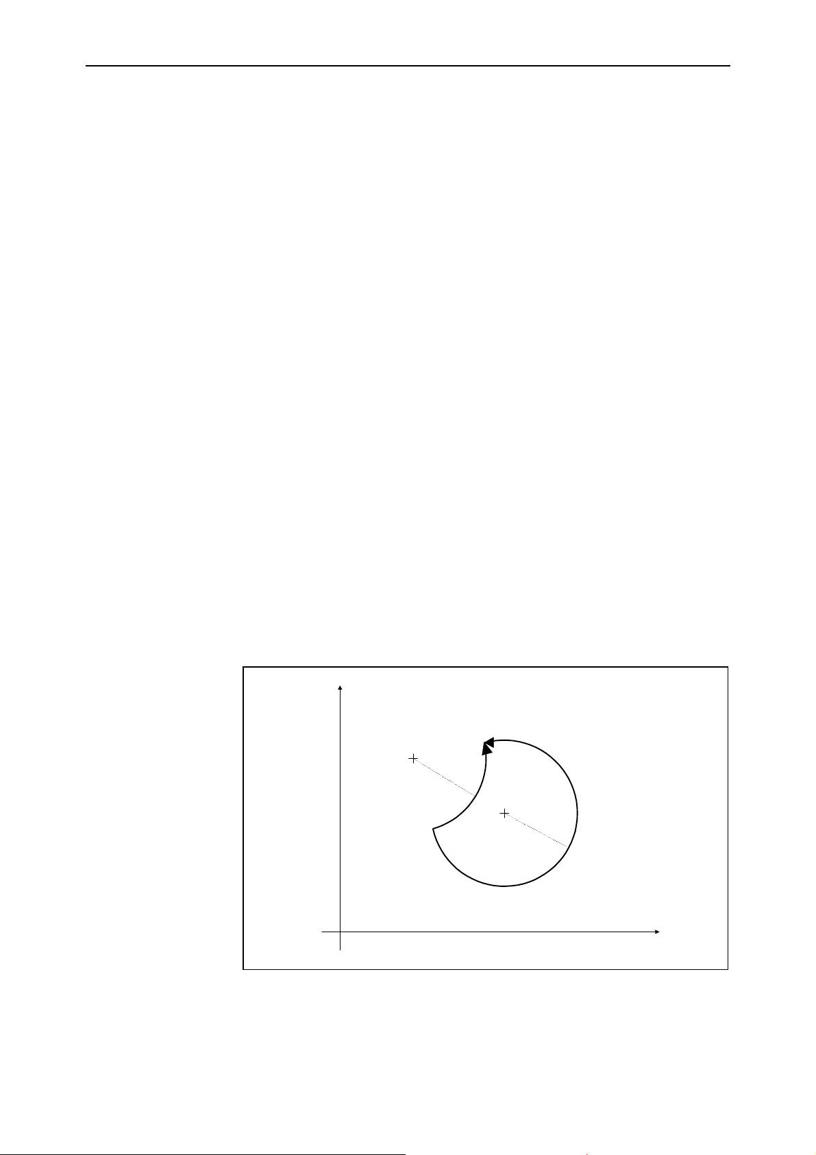
2.3.4 Circular interpolation

Syntax

Type of function

Description

Example

G2 (clockwise)
G3 (counterclockwise)

Modal, mutually exclusive with G0, G1, G33, G63

Circular interpolation drives the axes to the target point (within the fine tolerance
threshold) through a circular arc in the working plane at the speed set with parameter F.
The arc is defined by the target point and the centre coordinates (codes I, J and K) or by
the radius (code R).
The centre coordinates can be specified either absolutely or incrementally relative to the
starting point of the arc, depending on which mode is selected.
If the target point is set outside the plane of the arc, the actual path followed by the axes
becomes helical.
When programming the radius, an arc of angle greater than 180°° must be specified with
a negative sign.
G2-G3 cannot be used with more than 4 axes currently selected as feed axes.

G0 X0.0 Y0.0 (rapid feed to point P1(X0,Y0))
G2 F100 X100 Y0 I50 J0 (Clockwise circular arc to point
P2(X100, Y0) with centre C(X50, Y0))
G3 X0 Y0 R50 (Rcircular arc as above but
counterclockwise and defining the
radius (50) rather than the centre)
G2 X100 Y0 Z100 I50 J0 (Same arc, with change of plane
(helical))

Y

P2

R

P1

G3

-R

G3

Figure 2.4 - Circular interpolation with positive/negative radius

91752.DP.1.GB Esa/Gv2.16

X

DP Standard Programming

See also

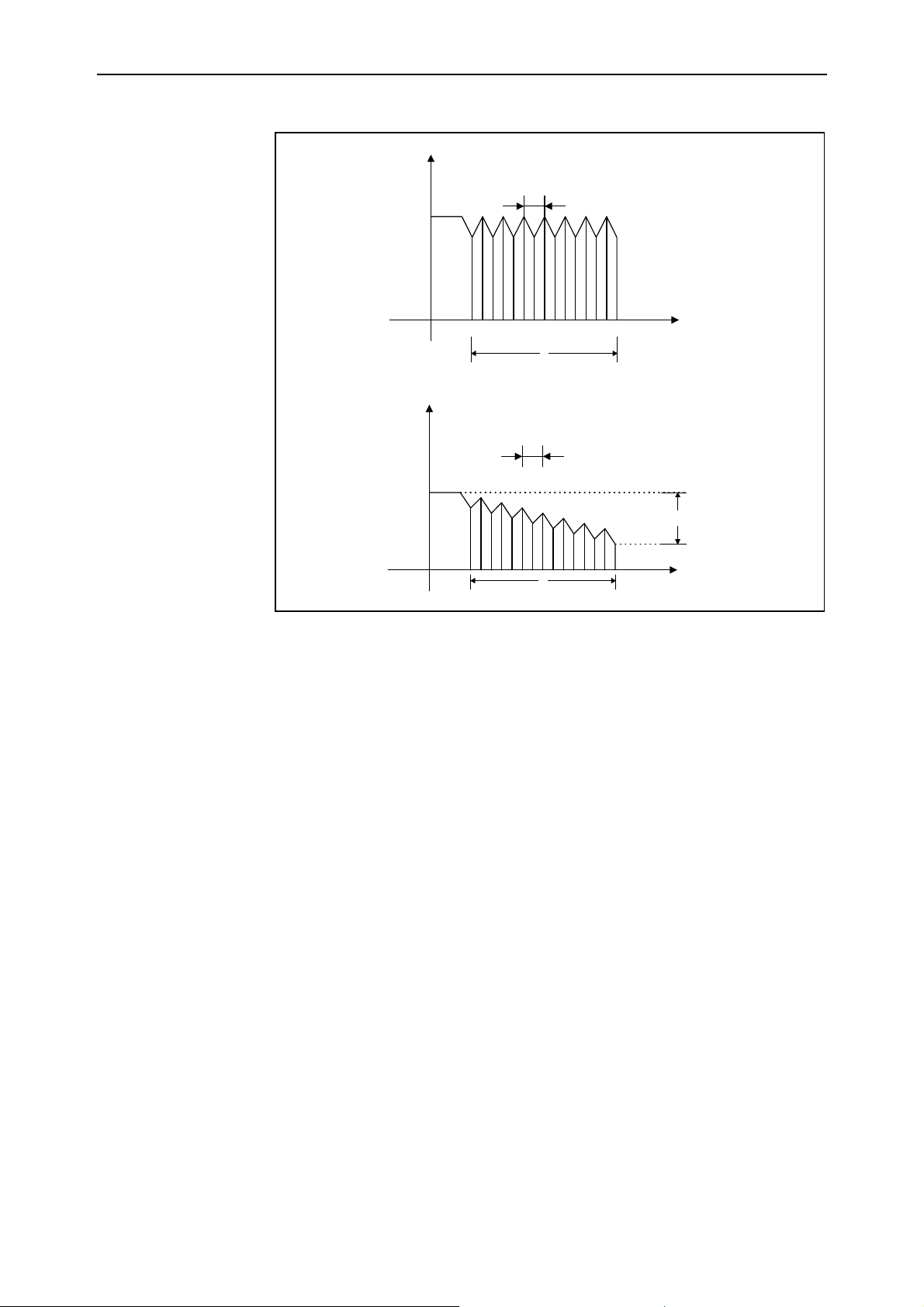
2.3.5 Thread-cutting

Syntax

Type of function

Description

Interpolation parameters, Feed command,Selecting the work plane.

G33 Zpos Kpitch (cylindrical)
G33 Zpos Xpos Kpitch (conical)

Modal, mutually exclusive with G0, G1, G2, G3, G63

Cuts a cylindrical, conical or planar thread from the current position to the programmed
target point, with the programmed pitch.
Not possible if one of the following functions is enabled: G95, G96.
During thread-cutting the spindle must be fitted with a position transducer.
The feed speed of each axis depends on the spindle speed (set by parameter S) and the
thread pitch.
The spindle's starting angle for thread-cutting is always zero.

Zpos
Kpitch

final longitudinal point
constant thread pitch

Example

See also

Xpos

S200 M3 (start spindle)
G0 X20 Z100 (approach to workpiece)
G33 Z70 K2 (cylindrical thread depth 30 mm with pitch

2)
G0 X30 (withdraw from piece)

Interpolations parameters,Tapping.

final radial point

Esa/Gv 91752.DP.1.GB 2.17

Standard Programming DP

x

K

z

Z

x

K

Z

Figure 2.5 - Geometric thread-cutting parameters G33

X

z

91752.DP.1.GB Esa/Gv2.18

DP Standard Programming

2.3.6 Tapping

Syntax

Type of function

Description

Example

G63 Zpos Kpitch

Modal, mutually exclusive with G0, G1, G2, G3, G33

Executes rigid tapping from current to programmed target point, with programmed pitch.
During tapping the spindle must be fitted with a position transducer.
The spindle speed is set by the parameter S. The longitudinal feed speed depends on the
spindle speed and the tapping pitch.
If the pitch is positive the spindle rotates clockwise for increasing Z and
counterclockwise for decreasing Z (righthand thread); vice versa for negative pitch.

Zpos
Kpitch

M19 (orient spindle)
S200 (select spindle speed)
G0 Z100 (approach to workpiece)
G63 Z70 K-2 (righthand tapping depth 30 mm with pitch 2)
G4 F0.2 (halt for 2 tenths)
G63 Z100 K-2 S1000(extract tool)
G0 Z200 (withdraw from workpiece)

end point

See also

Interpolation parameters,Thread cutting.

Esa/Gv 91752.DP.1.GB 2.19

Standard Programming DP

2.3.7 Timed halt

Syntax

Type of function

Description

Example

See also

G4 Ftime

Self-cancelling, mutually exclusive with G0, G1, G2, G3, G33, G63

The timed halt function stops the machine for the time set in the parameter F.

Ftime

G4 F2.5 (halt for 2.5 seconds)
X100 Y200 (feed to point P2(X100,Y200))

Positioned halt.

2.3.8 Positioned halt

Syntax

G9

[sec]

Type of function

Description

Example

See also

Self-cancelling

The positioned halt function forces stopping at the programmed point within the fine
tolerance threshold (set in the machine parameters) in rapid feed mode, in which the
rough tolerance would normally apply to allow passage to the next block.

G0 G9 X100 Y200 (feed to point P1(X100,Y200) with fine
tolerance)

Rapid feed,Timed halt.

91752.DP.1.GB Esa/Gv2.20

DP Standard Programming

2.4 Special interpolations

2.4.1 Auxiliary axis interpolations

Descriptin

Example

Interpolations can be programmed using the auxiliary axes UVW just as with the
cartesian axes XYZ (see G0, G1, G2, G3, G33, G63, G133).
Just as with the cartesian parameters, we can also apply tool radius and length
corrections, machining allowance (SVR/SVL), inverse feed programming (G93) and
selection of the system of reference (G58-G59).

To decide which axes are involved in the tool radius correction, for example, the system
first checks for the cartesian axes of the selected plane and if they are not enabled
checks for the corresponding auxiliary axes, finally checking the rotary axes.
If plane G17 is active, for example, and the axes YUVWA are currently enabled (that is,
they are in the current axis template, not disabled by CON[]=0), U and Y will be
selected for tool radius correction.
They are selected with the following priority:
cartesian axes XYZ => auxiliary axes UVW => polar axes ABC.

F100
D1
CON[A] = 0
G16 U Y Z+
G0 U0 Y0 Z0
G2 U200 Z30 R100
G0 U0 Y0 Z0
D0
G0 U0 Y0 Z0
D1
G16 W X Y+
G0 W0 X0 Y0
G2 W200 X0 Y30 R100
G0 W0 X0 Y0

2.4.2 Cylindrical programming

Description

Esa/Gv 91752.DP.1.GB 2.21

It is possible to interpolate with the linear axes XYZ UVW and at the same time with the
polar axes ABC (v. G0, G1, G2, G3).

When programming circular interpolations with one linear and one polar axis, we have
adopted an approach of the type "mm = degrees": the polar coordinates are programmed
in degrees, but the CNC interprets them as mm. In other words, although the polar
coordinates are degrees, they are also mm in practice if the operator has calculated the
position correctly in degrees (that is multiplying the position in mm by 57.299 and
dividing by the radius of the cylinder).
To avoid rejection of the machining operations by the CNC (which checks whether the
parameters specified with G02 actually result in a circle) the coordinates must always be
in degrees (which the slave interprets as mm) compatible with the mm specification.
This approach means that, if the numerical information is correct but the operator has
not correctly converted from degrees to mm, the interpolation arc is a segment of an
ellipse.

Standard Programming DP

Furthermore, the radius of the cylinder can be unknown, and therefore a special mode is
not required for cylindrical programming: the ABC axes can be interpolated as if they
are cartesian. Note that the radius of the cylinder must be known to the operator doing
the calculations, however.
Finally, this mode conforms to the modular arithmetic (mod 360) of the cylinder,
inasmuch as the polar coordinates are programmed in degrees.

Example

F1000
D1G16 B Y X+
G42
G01 Y0 B0
G01 Y120
B30
G93 F2 G02 Y90 B60 R30
G01 Y70
G03 Y60 B70 R10
G01 B150
G03 Y70 B190 R75
G01 Y110 B230
G02 Y120 B270 R75
G01 B360
G40
G58 Y200
G41
G94 F1000
G01 Y0 B0
G01 Y120
B30
G93 F2 G02 Y90 B60 R30
G94 F1000
G01 Y70
G03 Y60 B70 R10
G01 B150
G03 Y70 B190 R75
G01 Y110 B230
G02 Y120 B270 R75
G01 B360
G40

See also

Programming the feed, Feed command, Rapid feed, Linear interpolation,Circular
interpolation.

91752.DP.1.GB Esa/Gv2.22

DP Standard Programming

2.5 Spindle orientation

2.5.1 M19: Spindle orientation

Syntax

Type of function

Description

Example

See also

M19 Sangle

Self-cancelling

Orients the spindle. The angle of orientation of the spindle is set with the S parameter or,
if this is not available, is defined in the machine parameters.
The spindle must be fitted with a position transducer.
The speed of rotation for spindle orientation is defined in the parameters.
This is a closed loop positioning command, which corresponds to the positioning of a
polar axis.

Sangle

M19 S45(orient the spindle at 45°)

On the fly spindle orientation.

Esa/Gv 91752.DP.1.GB 2.23

Standard Programming DP

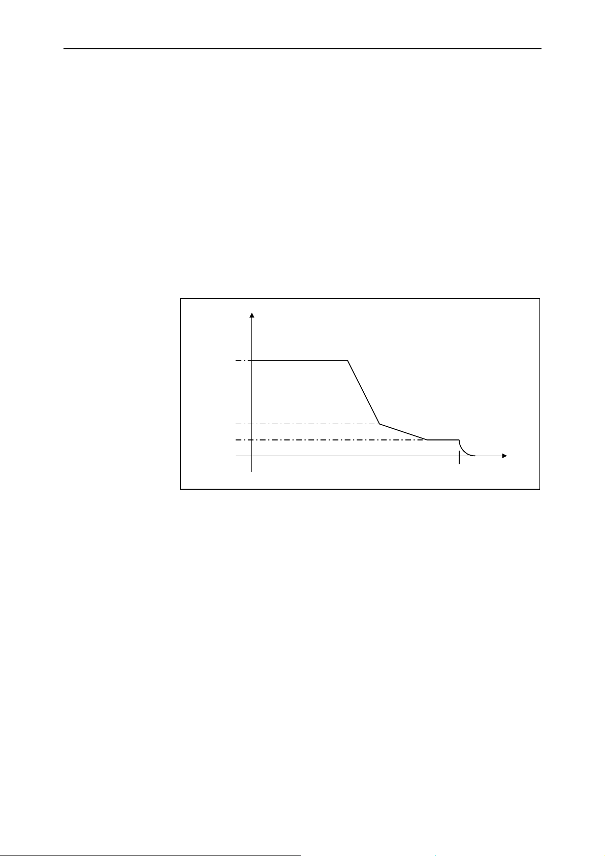
2.5.2 On-the-fly spindle orientation

Syntax

Description

M19 Sangle

On-the-fly orientation enables switching from a closed to an open loop. If the spindle is
rotating in an open loop it can be oriented without having to first stop it.
Phase 1) the PLC zeroes the rotation bit
Phase 2) the spindle decelerates to Vdec
Phase 3) the process assumes the programmed acceleration and decelerates to Vstop.
Phase 4) Vstop is maintained until the position error generates the current output
voltage.
Phase 5) the loop closes and positioning occurs.
*) In the current version Vstop = Vdec (SP_VELM19) so the acceleration change in
Phase 3 does not occur.

Vdac

Vmax

Vdec

Vstop

Example

See also

Close ring

T

Figure 2.6 - Spindle speed control during on-the-fly orientation

S1500 M3 ;Open loop rotation
M19 S45.0 ;Closed loop orientation on-the-fly orientation

S1500 M3 ;Open loop rotation
M5 ;Stop spindle
M19 S45.0 ;Orient spindle Preceding mode

M19: spindle orientation.

91752.DP.1.GB Esa/Gv2.24

DP Standard Programming

2.6 Programming axis and spindle speed

2.6.1 Setting the feed rate

Syntax

Type of function

Description

Fspeed

Modal

The F parameter sets the interpolation feed rate.
The feed rate is normally expressed in mm/min, but in the case of polar axes the rate is
expressed in degrees/min. There is also a mode (G95) in which the feed rate is expressed
in mm/revs.
If all axes are cartesian the feed rate for the interpolation is expressed in mm/min (in
G94 mode).

For a single polar axis the feed rate is expressed in degrees/min (in G94 mode).

If all axes are polar the unit is still degrees/min (in G94 mode) bearing in mind that the
feed rate applies to a n-dimensional vector whose components are the angles of travel in
the various polar axes.

If we want the two polar axes A and B to travel through 30° (∆A) and 40° (∆B)
respectively in 0.20min (t), we first calculate the modulus of the vector (in this case two
dimensional) (S, angle of travel in degrees):

2

∆

S

∆

A

B230240250

then we divide by the time (t) to obtain the angular speed (V) in degrees/min:

St50

V

250.0

0.20

If both cartesian and polar axes are being used together, the cartesian coordinates are
programmed in mm/min (in G94 mode).
The polar axes interpolate linearly over the same time of travel required by the cartesian
coordinates.

This type of programming is typical of applications which require:
ù a tool tangential to the yaw axis (e.g.: non-contour glass cutting with head tangential

to plane);

ù a polar axis whose rate is not predominant (i.e. negligible relative to the cartesian

feed rate).

In the following situations:
ù the travel of the X and Y axes is zero or too small to allow modulation of the polar

axis feed rate with the required precision;

Esa/Gv 91752.DP.1.GB 2.25

Standard Programming DP

ù the n-dimensional vectorial speed must be computed separately, as the components

are not commensurable (linear and angular travel); using the option "programming
the feed rate as inverse feed" G93.

Examples

G0 X100 Y100 (feed to point P1(X100,Y100))
G1 Y200 F500 (linear to point P2(X100,Y200) with feed rate
500 mm/min)

G00 X0.000 Y0.000
G01 X30.000 Y40.000 F25.0

G00 A0.000 (*** ONE SINGLE POLAR AXIS ***)
G01 A30.000 F3000 (polar axis feed rate 3000 degrees/min)

G00 A0.000 B0.000 (*** SEVERAL POLAR AXES ***)
G01 A30.000 B40.000 F250.0 (see example on previous page)

G00 X0.000 Y0.000 A0.000 (*** COMBINED CARTESIAN AND POLAR
AXES ***)
G01 X30.000 Y40.000 A20.000 F25.0 (feed rate in mm/min)

G00 A0.000 B0.000 (*** Inverse feed ***)
G93 F250.0 G01 A30.000 B40.000 (positioning in 1/250 sec)

See also

Linear interpolation, Inverse feed, Timed halt.

2.6.2 Continuous feed mode

Syntax

Type of function

Description

G64 (enable)
G61 (disable)

Modal, disabled by default

In continuous feed mode the system passes from one block to the next without stopping
the axes.
There are, however, some commands which interrupt the continuous cycle and stop the
axes at the end of the block, such as G4, G9, M and T.
Disabling continuous feed implies stopping the axes at the end of the block which
contains the command G61 itself.

Example

See also

G0 X100 Y100 (feed to point P1(X100,Y100))
G1 G64 Y200 F500 (linear to point P2(X100,Y200) no halt)
G2 G61 X200 R50 (circular arc to point P3(X200, Y200) with
halt)

Setting the feed rate,Continuus feed mode with speed look ahead.

91752.DP.1.GB Esa/Gv2.26

DP Standard Programming

2.6.3 Continuous feed mode with speed look-ahead

Description

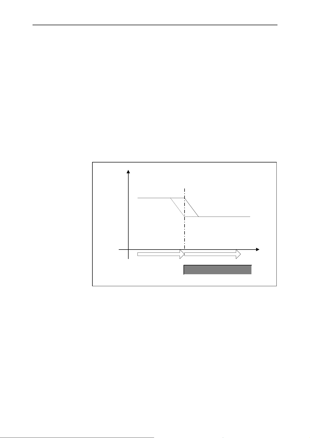
The machine parameters allow enabling speed look-ahead
[Channel parametersàOption: Speed Look Ahead].

If speed look-ahead is enabled in continuous feed mode the speed changes continuously
to meet that of the next section, i.e.:

Vout[K] = Vmax[K+1]

The approach to the piece is usually determined by a G0 (positioning), while the actual
machining is carried out by interpolation, G1,G2,G3. In continuous feed mode the
transition from one feed rate to another sometimes has undesired effects in the
machining of the piece. Enabling speed look-ahead makes it possible to anticipate the
transition and thus allows smooth machining of the piece..

Vdac

speed look ahead

VG0

VG1

speed look ahead

enabled

disabled

Example

TG1G0

Workpiece

Figure 2.7 - Feed rate transition with/without look-ahead

;LOOK AHEAD ENABLED
;******* REPORT *******
F10000 G64

G0 Y500 X100 ;Vmaxà833333 Voutà166666
G1 X1000 ;Vmaxà166666 Voutà166666

G61
G1 X1000 ;Vmaxà166666 Voutà0

;LOOK AHEAD DISABLED
;******* REPORT *******
F10000 G64

Esa/Gv 91752.DP.1.GB 2.27

Standard Programming DP

G0 Y500 X100 ;Vmaxà833333 Voutà833333
G1 X1000 ;Vmaxà166666 Voutà166666

G61
G1 X1000 ;Vmaxà166666 Voutà0

See also

Continous feed mode.

2.6.4 Selecting the feed mode

Syntax

Type of function

Description

G94 (feed rate in mm/min)
G95 (feed rate in mm/rev)

Modal, in mm/min by default

The feed rate is defined by the parameter F and can be absolute (in mm/min) or relative
to the spindle rotation speed (in mm/rev).
If the spindle is not fitted with a position transducer, the nominal rotational speed is used
in mm/rev mode.

Using G95, which allows interpretation of the F values as mm/rev, subordinates the rate
of the linear axes to the speed of the spindle itself. If the spindle speed increases, so does
that of the linear axes.

The vectorial feed rate is determined by the following formula

Example

See also

mm

V S F

= ∗

rpm

[ ]

min

where
S

is the speed of the spindle

rpm

F advance per rev set by G95

G0 X100 Y100 (feed to point P1(X100,Y100))
S1000 M3 (start spindle)
G95 F2.1 (enable feed in mm/rev)
G1 Y200 (linear to point P2(X100,Y200) with feed rate

bound to spindle speed à
1000 rpm *2.1mm/rev = 2100 mm/min)

Settinf the feed rate,Setting the spindle rotation mode.

91752.DP.1.GB Esa/Gv2.28

DP Standard Programming

2.6.5 Selecting the spindle rotation mode

Syntax

Type of function

Description

Example

See also

Sspeed

Modal

Parameter S sets the speed of rotation of the spindle.
The speed is usually expressed in rpm, but there is a mode in which the speed is
expressed as cutting speed in m/min (G96).

Speed speed of rotation, rpm or m/min

S500 M3 (start spindle clockwise at 500 rpm)

Setting the spindle rotation mode..

2.6.6 Setting the spindle rotation mode

Syntax

Type of function

Description

G96 (constant cutting speed)
G97 (constant rpm)

Modal, constant rpm by default (G97)

This function keeps the cutting speed constant, thus optimising the machining quality.
The speed of rotation of the spindle is set with the parameter S and can be absolute (in
rpm) or relative to the position of the linear axis with which it is associated, for example
X (cutting speed in m/min).
This function is characteristic of lathes, in which the position of the X axis determines
the diameter of the piece at the point of machining.

The speed of the spindle cannot exceed a maximum.
When constant cutting speed mode is disabled the speed of rotation of the spindle stays
constant at the most recent value.

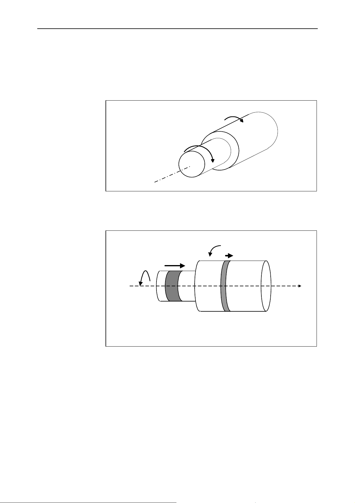
Selecting G96 forces interpretation of S as m/min, and to keep the cutting speed constant
the spindle speed must be modulated by the radius of the contour, for example, if the
radius decreases, the spindle speed increases.

m

S

[ ]

min

G

V rpm

MAND

[ ]

96

=

R m

[ ]

2

π

Esa/Gv 91752.DP.1.GB 2.29

Standard Programming DP

where
R is the position on the linear axis,
S

is the constant cutting speed set with G96

G96

From the above relation we can see that the speed of the spindle is inversely
proportional to the position R.

Spindle speed

down

Spindle speed

up

Figure 2.8 - G96 variation of the speed according to the turning radius

This mode can be combined with G95 which programs F in mm/rev, so as to ensure
covering constant areas in constant time.

S'

rpm

V'

V

S

rpm

A

Y

A'

Figure 2.9 - G95-G96 Constant area machining

From the figure it is evident that with constant cutting speed the following relation holds

S

> S'

rpm

rpm

If we program with G95, the linear feed rate V is proportional to S so that

V> V
In this case, in a certain interval of time ∆t, the machined area is given by:

91752.DP.1.GB Esa/Gv2.30

DP Standard Programming

Example

A=2πr × V∆t = 2πr × f(S
A'=2πR × V'∆t = 2πR × f(S'

)∆t = 2πr × f(g(1/r))∆t

rpm

)∆t =2πR × f(g(1/R))∆t

rpm

where f(S)=K × S and S= g(1/r)= K' × 1/r
A=A'= 2π × const

(* enable constant cutting speed with G96)

G0 X100 Y100 (*X radius)
S500 M3 (*spindle at 500 rpm)
G96 S100 (*constant cutting speed 100 m/min

spindle:159 rpm à X=100)
G4 F1

G1 X50 Y50 F1000 (*spindle at 318 rpm à X=50 )
G97
G4 F1
S500 (*spindle at 500 rpm )
G4 F1
M5 (*stop spindle)

(* enable G95 and G96 simultaneously)

G0 X100 Y100
S500 M3 (*spindle at 500 rpm )
G96 S100 (*spindle at 159 rpm )
G4 F5
G95 F1 (*temporary 159 mm/min --> Vmax=2650 Hz)
G1 X50 (*spindle at 318 rpm speed 318 mm/min
Vmax=5300Hz)
G1 Y50 (*speed 318 mm/min --> Vmax=5300Hz)
G97 G94
G4 F1
S500 (*spindle at 500 rpm )
G4 F1
M5
M30

See also

Selecting the spindle rotation mode.

Esa/Gv 91752.DP.1.GB 2.31

Standard Programming DP

2.6.7 Inverse feed

Syntax

Type of function

Description

G93 F < inverse_feed >

Modal, exclusive with G94 and G95, disabled when the CNC is switched on.

1

Where inverse_feed, expressed in

min

, is the ratio:

V

F

=

L

V is a speed expressed in any units over time.
L is the length of the section in the same units.

from which the units for the parameter F are:

u













min

= =

u

Selects, for the current block, the speed as the inverse (or reciprocal) of the time.

min

min

−11

Applications

Example

"Inverse feed" is enabled with G93, for instance:
ù when programming both polar and linear axes in the same block and the travel of

the linear axes is zero or too small for the polar axes to be modulated with the
required accuracy;

ù when the velocity must be programmed externally as an n-dimensional vector with

incommensurable components (e.g.: spaces and angles).

A is the yaw axis of the spindle which results in a large displacement of the tool point in
contact with the piece even with small angular displacements. To program an operation
which involves axes X, Y, Z and A, with a suitable feed rate. The travel of the linear
axes is extremely limited so that the physical speed of the fourth axis cannot be
accurately regulated(and hence neither can the speed of the tool point) using normal
mm/min programming. This type of feed can be extracted from a CAD/CAM program,
using calculations which take into consideration the tool point path and the axis
movements.
In this case we use inverse feed programming (G93).

The axes must move from:

X0.000 Y0.000 Z0.000 A0.000

to:

X0.010 Y0.010 Z0.023 A100.000

91752.DP.1.GB Esa/Gv2.32

DP Standard Programming

interpolating linearly.

We know the path of the tool point during interpolation (different from the XYZ axis
paths):

400 mm

We know the linear feed rate of the tool point during the interpolation:

1600 mm/min

We program G93 with the speed:

1600

F = =

4

400

(the reciprocal of the feed time, 0.25min)

We thus obtain:

G00 X0.000 Y0.000 Z0.000 A0.000
G93 F4 G01 X0.010 Y0.010 Z0.023 A100.000 (positioning in ¼
of a second)
G94 F1000 (resets the speed to mm/min)Auxiliary functions

Esa/Gv 91752.DP.1.GB 2.33

Standard Programming DP

2.7 Polar axes programming

2.7.1 Polar axes with travel limitation

The targets expressed are absolute and range from the minimum target to the maximum
one, inclusive. In relation to the distance covered, the behaviour is the same as that for a
Cartesian axis.

e.g.:

G0 C-90.000
G0 C270.000 ; The axis moves forwards through 360
degrees

G0 C315.000
G1 F5000 C45.000 ; The axis moves backwards through 270
degrees

G0 C45.000
G1 F3000 C315.000 ; The axis moves forwards through 270
degrees

2.7.2 Round axes

Operation in the rapid
mode

The behaviour described can be modified by means of certain operators that allow the
direction and rpm rate of the polar axis to be conditioned. See the Selection of the
direction and rpm rate section. Note, in that section, how the behaviour described is the
same as that of the AC operator.

Depending on the counting method, the programmed target determines the position to
reach and not the absolute target of the axis. If the target is beyond the [0..mod) range,
it is brought back within that range.

The direction is therefore determined so as to reach the programmed position via the
shortest possible route. If the programmed position is the same as the one in which the
axis actually is, the axis remains at a standstill.

e.g.:

G0 C-90.000
G0 C270.000 ;The axis remains at a standstill

G0 C315.000
G0 C45.000 ; The axis moves forwards through 90 degrees

G0 C45.000
G0 C315.000 ; The axis moves backwards through 90 degrees

The behaviour described can be modified by means of certain operators that allow the
direction and rpm rate of the polar axis to be conditioned. See the Selection of the

91752.DP.1.GB Esa/Gv2.34

DP Standard Programming

direction and rpm rate section. Note, in that section, how the behaviour described is the
same as that of the DC operator.

Operation in the feed
mode

If a target is programmed within the [0..mod) range, the axis will reach the required
position without passing via 0. E.g.:

G0 C-90.000
G1 F5000 C270.000 ; The axis remains at a standstill

G0 C315.000
G1 F5000 C45.000 ; The axis moves backwards through 270
degrees

G0 C45.000
G1 F5000 C315.000 ; The axis moves forwards through 270
degrees

A target beyond the [0..mod) range can also be programmed without any limitations. In
that case, the distance to cover is determined by considering the programmed target and
the current position, only this latter within the [0..mod) range. After the block has been
executed, the programmed target will be brought back within the [0..mod) range and will
form the new current position. This means that if targets beyond the [0..mod) range are
programmed for a round axis, they will always result in movement of the axis, regardless
of the current position.
E.g.:

G0 C45.000
G1 F5000 C405.000 ; The axis moves forwards through 360
degrees

G1 C405.000 ; The axis moves again forwards through 360
degrees

G1 C45.000 ; The axis remains at a standstill
G1 C-315.000 ; The axis moves backwards through 360
degrees

G1 C-315.000 ; The axis moves again backwards through 360
degrees

G1 C45.000 ; The axis remains at a standstill

Esa/Gv 91752.DP.1.GB 2.35

Standard Programming DP

2.7.3 Selection of the direction and rpm rate

Certain operators are available for conditioning the direction and rpm rate of the polar
axis. These operators are implemented like a series of functions that produce values
which must be assigned to the address of the polar axes for which conditioned
movement is required. For example:

G0 C=DC(45.000)
G1 F5000 C=ACP(1,45.000)

These operators have the same effect on blocks executed in the rapid and feed modes.

Incremental
positioning (IC)

Absolute positioning
(AC)

<polar axis>=IC(<Incremental target>)

Es.:

C=IC(-25.000)

The axis is moved so as to cover the distance defined by <incremental_target> in the
positive or negative direction, depending on the sign. The target reached will be given
by the algebraic sum of the current target and <incremental_target>, brought back
within the [0..mod) range in the case of a round axis.

<polar_axis>=AC(<absolute_target>)

E.g.:

C=AC(45.000)

In the case of axis with travel limitation, <absolute target>, it is expressed within the
minimum target and maximum target range, inclusive. In relation to the distance
covered, the behaviour is the same as that for a Cartesian axis. For example:

C=AC(-90.000)
C=AC(270.000) ; The axis moves forwards through 360
degrees

C=AC(315.000)
C=AC(45.000) ; The axis moves backwards through 270
degrees

C=AC(45.000)
C=AC(315.000) ; The axis moves forwards through 360
degrees

In the case of a round axis, and if an <absolute_target> value is programmed within the
[0..mod) range, the axis will reach the required position without passing via 0. E.g.:

C=AC(-90.000)
C=AC(270.000) ; The axis remains at a standstill

C=AC(315.000)
C=AC(45.000) ; The axis moves backwards through 270
degrees

91752.DP.1.GB Esa/Gv2.36

DP Standard Programming

C=AC(45.000)
C=AC(315.000) ; The axis moves forwards through 270
degrees

Again in the case of a round axis, and <absolute_target> value can also be programmed
beyond the [0..mod) range without any limitations. In this case, the distance to cover is
determined considering the <absolute_target> and the current position, only this latter
within the [0..mod) range. After the block has been executed, the <absolute_target>
will be brought back within the [0..mod) range and will form the new current position.
This means that programming an AC function with <absolute_target> values beyond
the [0..mod) range for a round axis will always result in movement of this latter,
regardless of the current position.
E.g.:

C=AC(45.000)
C=AC(405.000) ; The axis moves forwards through 360 degrees

C=AC(405.000) ; The axis moves again forwards through 360
degrees

C=AC(45.000) ; The axis remains at a standstill
C=AC(-315.000); The axis moves backwards through 360
degrees

Absolute positioning
with the least
distance (DC)

C=AC(-315.000); The axis moves again backwards through 360
degrees

C=AC(45.000) ; The axis remains at a standstill

<polar_axis>=DC(<absolute_position>)

E.g.:

C=DC(45.000)

Depending on the counting module, <absolute_position> determines the position to
reach and not the absolute target of the axis. If <absolute_position> is beyond the
[0..mod) range, it will be brought back within this range.

The direction is therefore determined so as to reach the programmed position via the
shortest possible route. If the programmed position is the same as the one in which the
axis actually is, the axis remains at a standstill.

E.g.:

C=DC(-90.000)
C=DC(270.000) ; the axis remains at a standstill

C=DC(315.000)
C=DC(45.000) ; The axis moves forwards through 90 degrees

C=DC(45.000)
C=DC(315.000) ; The axis moves again backwards through 90
degrees

In the case of axis with travel limitation (module 360):

Esa/Gv 91752.DP.1.GB 2.37

Standard Programming DP

C=AC(765.000) ; The position of the axis will be 45 degrees
(765 MOD 360)
C=DC(315.000) ; The axis moves forwards through 90 degrees
and reaches the position of 675

Absolute positioning
in the positive
direction (ACP)

<polar axis>=ACP(<absolute_position>)
<polar axis>=ACP(<n_rev>,<absolute_position>)

E.g.:

C=ACP(45.000)
C=ACP(2,45.000)

Depending on the counting module, <absolute_position> determines the position to
reach and not the absolute target of the axis. If <absolute_position> is beyond the
[0..mod) range, it will be brought back within this range.

The required position is reached by moving the axis in the positive direction. If the
programmed position is the same as the one in which the axis actually is, the axis
remains at a standstill.
E.g.:

C=DC(-90.000)
C=DC(270.000) ; the axis remains at a standstill

C=DC(315.000)
C=ACP(45.000) ; The axis moves forwards through 90 degrees

C=DC(45.000)
C=ACP(315.000) ; The axis moves forwards through 270
degrees

In the case of axis with travel limitation (module 360):

C=AC(765.000) ; The position of the axis will be 45
degrees(765 MOD 360)

C=ACP(315.000); The axis moves forwards through 270 degrees
and reaches the position of 1035

An additional number of revolutions can be expressed <n_rev>. If programmed, the
<absolute_position> reached will be the same, but the required number of revolutions

will be added to the distance normally covered to reach it in the positive direction.

C=DC(-90.000)
C=ACP(1,270.000) ; The axis moves forwards through 360
degrees

C=DC(315.000)
C=ACP(1,45.000) ; The axis moves forwards through 450
degrees

C=DC(45.000)
C=ACP(1,315.000) ; The axis moves forwards through 630
degrees

91752.DP.1.GB Esa/Gv2.38

DP Standard Programming

In the case of axis with travel limitation (module 360):

C=AC(765.000) ; The position of the axis will be 45
degrees(765 MOD 360)

C=ACP(1,315.000) ; The axis moves forwards through 630
degrees and reaches the position of 1395

Absolute positioning
in the negative
direction (ACN)

<polar axis>=ACP(<absolute_position>)
<polar axis>=ACP(<n_rev>,<absolute_position>)

E.g.:

C=ACN(45.000)
C=ACN(2,45.000)

Depending on the counting module, <absolute_position> determines the position to
reach and not the absolute target of the axis. If <absolute_position> is beyond the
[0..mod) range, it will be brought back within this range.

The required position is reached by moving the axis in the positive direction. If the
programmed position is the same as the one in which the axis actually is, the axis
remains at a standstill.
E.g.:

C=DC(-90.000)
C=DC(270.000) ; the axis remains at a standstill

C=DC(315.000)
C=ACN(45.000) ; The axis moves backwards through 270
degrees

C=DC(45.000)
C=ACP(315.000) ; The axis moves backwards through 90
degrees

In the case of axis with travel limitation (module 360):

C=AC(765.000) ; The position of the axis will be 45
degrees(765 MOD 360)

C=ACN(315.000); The axis moves forwards through 90 degrees
and reaches the position of 675

An additional number of revolutions can be expressed <n_rev>. If programmed, the
<absolute_position> reached will be the same, but the required number of revolutions

will be added to the distance normally covered to reach it in the positive direction.

C=DC(-90.000)
C=ACN(1,270.000) ; The axis moves backwards through 360
degrees

C=DC(315.000)
C=ACN(1,45.000) ; The axis moves backwards through 630
degrees

C=DC(45.000)

Esa/Gv 91752.DP.1.GB 2.39

Standard Programming DP

C=ACP(1,315.000) ; The axis moves backwards through 450
degrees

In the case of axis with travel limitation (module 360):

C=AC(765.000) ; The position of the axis will be 45
degrees(765 MOD 360)

C=ACN(1,315.000) ; The axis moves forwards through 450
degrees and reaches the position of 315

2.7.4 Speed programming in the presence of polar axes

Interpolation with one
or more Cartesian
axes and no polar
axis

Interpolation with one
or more polar axes
and noCartesian axis

Only polar axis

MORE polar axes

The speed is programmed on the trajectory described by the Cartesian axes in mm/min
(in the G94 mode).

E.g.:

G00 X0.000 Y0.000
G01 X30.000 Y40.000 F5000

The speed polar axis is programmed in mm/min (in the G94 mode).

Es.:

G00 C0.000

G01 C30.000 F3000

Programming is always carried out in degrees/min (in the G94 mode) considering,
however, that the speed acts on an n-dimensional vector whose components on the
various dimensions are the angles covered by the polar axes.
If two polar axes A and B must cover angles of 30° (∆A) and 40° (∆B), respectively,
taking 0.20min, (t), first calculate the first module of the vector, two-dimensional in this
case (S, angle covered in degrees):

2

∆

ù

S

∆

A

B230240250

then, divide by the time (t) to obtain the angular velocity (V) in degrees/min:

St50

V

ù

250.0

0.20

91752.DP.1.GB Esa/Gv2.40

DP Standard Programming

Now program:

G00 C0.000 B0.000
G01 C30.000 B40.000 F250.0

Interpolation in the
presence of both
Cartesian and polar
axes

Programming the
speed as time
reciprocal

The speed is programmed on the trajectory described by the sole Cartesian axes in
mm/min (in the G94 mode).

The polar axes interpolate linearly in the same time taken by the Cartesian axes.

E.g.:

G00 X0.000 Y0.000 A0.000
G01 X30.000 Y40.000 C20.000 F2500

In certain situations, it may be more convenient to program the speed as inverse of time,
by means of the G93 mode. This sort of situation may occur when the component on the
Cartesian axes is extremely small and the speed of the polar axes must be accurately
modulated.

In the G93 mode, no distinctions are made between the types of axes in a block since the
reciprocal of the travel time of the block is expressed and not a linear/angular space per
unit of time.

Esa/Gv 91752.DP.1.GB 2.41

Standard Programming DP

2.8 Auxiliary Functions

2.8.1 Functions M and T

M functions

The M auxiliary functions (miscellaneous) are generally plant-specific and are defined
by the machine manufacturer, (except for M2, M19 and M30).
When setting the M functions the following standards must be adhered to:

Function Meaning

M0 Unconditional halt
M1 Optional halt
M2 End of program (not redefinable)
M3 Clockwise spindle rotation
M4 Counterclockwise spindle rotation
M5 Spindle halt
M6 Tool change
M7 Coolant 1 ON
M8 Coolant 2 ON
M9 Coolant OFF
M10 Lock
M11 Unlock
M19 Spindle orientation (not redefinable)

T functions

M30 End of program (not redefinable)
M40 Automatic range change
M41 Select range 1
M42 Select range 2
M43 Select range 3
M44 Select range 4
M48 Reset override
M49 Override off
M60 Change piece

The M functions ensure synchronisation of the channel with the rest of the system, via
data interchange with the PLC.
The machine parameters allow selection of the control mode (Enable Overlapped M)
which enables reduction of deadtime due to waiting for synchronisation signals.

The T auxiliary functions specify and setup the tool to be fitted with the next M6
command.

91752.DP.1.GB Esa/Gv2.42

DP Standard Programming

The T function specifies the tool number, but has no bearing on tool compensation
which is handled by the D function.

Order of execution

The order of execution of commands in a given block is as follows:

ù T functions
ù S functions
ù M functions
ù Feed
ù Timing

A block may contain only one command of each type, except for the M functions, of
which there may be up to 3 in one block.

Esa/Gv 91752.DP.1.GB 2.43

Standard Programming DP

2.9 Tool compensation

2.9.1 Tool length correction

Tool corrector table

See also

The D function enables selection of the tool corrector, DD disables tool compensation.
The CNC contains a table which the operator can access, in which for every corrector a
set of data can be specified which defines the mode and properties of the tool
compensation. The 0 element of the table is not available. for example, if 10 tools are
defined in the defcn, the ones available are those from 1 to 9.

The command Dxx acquires the correction data for the tool and automatically enables
the length correction along the axis orthogonal to the machining operation. The tool
length is added to the position along the specified axis.
Note: before the Dxx function is used, it is obligatory to define the versors for both the
specified machining plane and the tool In the simplest case, where a machining
operation takes place on plane XY (G17) using a tool that works perpendicularly to the
plane along Z axis, it is always necessary to set the following versors:

EI0 EJ0 EK1
EP0 EQ0 ER1

Selecting the work plane, Tool radius compensation.

Versor for the machining plane
Versor for the tool

91752.DP.1.GB Esa/Gv2.44

DP Standard Programming

2.9.2 Tool radius compensation

Syntax

Type of function

Description

G40 (disables radius compensation)
G41 (enables radius compensation to the left of the tool path)
G42 (enables radius compensation to the right of the tool path)

Modal, disabled by default

Tool radius compensation enables contour milling on a plane with automatic
compensation of the tool's radius.
The value of the tool radius used to calculate the actual tool path is taken from the D
corrector for the tool.

Compensation is applied to the selected plane, hence by default on the XY plane(G17).

For correct tool radius compensation, proceed as follows:

ù select the appropriate tool corrector Dxx;
ù program G41or G42.

In active compensation mode:
ù Each feed command must involve at least one of the two plane axes, otherwise the

compensation algorithm will return an error.

ù The correction direction/milling plane cannot be modified without disabling the

compensation itself.

ù Two consecutive rapid feeds cannot be programmed.

Two contiguous tool paths, each with radius compensation, can be connected in a
different way:

ù if the two paths form a convex angle the two paths are connected by a circular arc,
ù if the two paths form a concave angle the first path is continued until it intersects the

projection of the second.

G40, which deactivates the compensation function, takes effect from the start of the next
machining segment.
The following two figures show tool paths with G41 and G42 correction using a flat end
mill.

Esa/Gv 91752.DP.1.GB 2.45

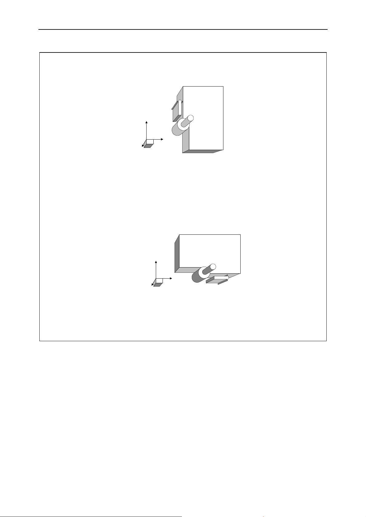
Standard Programming DP

G41

X

Y

Z

G42

X

Y

Z

Figure 2.10 - G42 correction with flat end mill:

91752.DP.1.GB Esa/Gv2.46

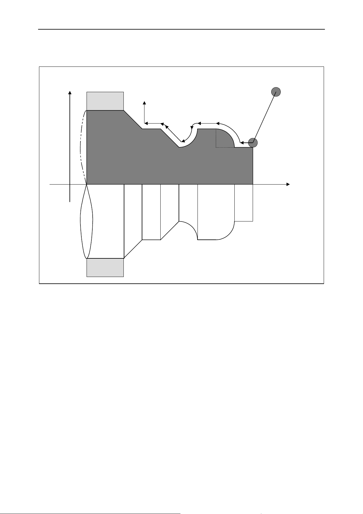
DP Standard Programming

The following figure shows G42 correction for a lathed part,

G18: ZX plan

X

Clamp

G1

G1

G1

G2

G1

G3

R

G1

G42

Z

Clamp

Figure 2.11 -Lathe tool correction:

Esa/Gv 91752.DP.1.GB 2.47

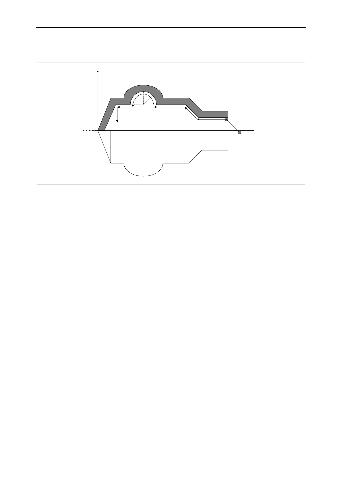
Standard Programming DP

and in the following for a bored part:

X

G3

R

G1G1

G1

G1

G1

G41

Z

Figure 2.12 - Boring tool correction

91752.DP.1.GB Esa/Gv2.48

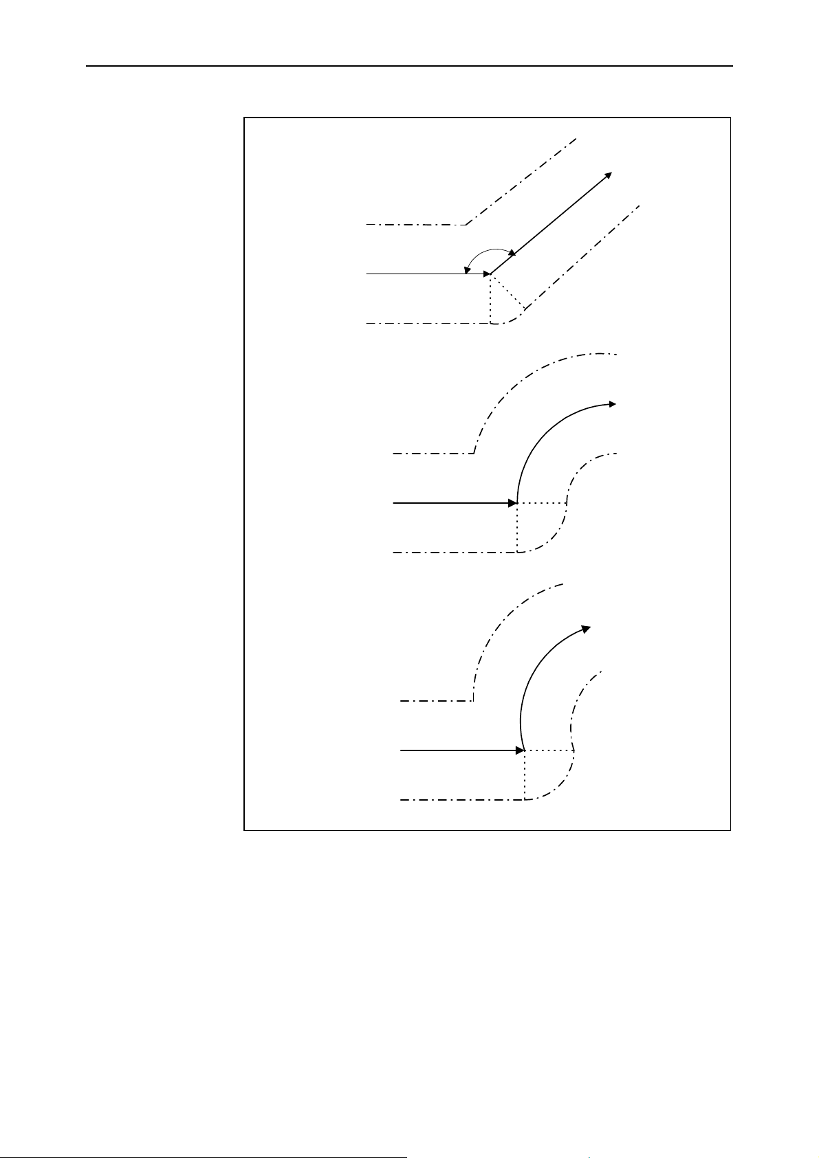
DP Standard Programming

G41

programmed
course

G42

G41

programmed
course

G42

G41

programmed
course

G42

Figure 2.13 - Tool compensation: programmed and corrected path

Interference check

The tool correction algorithm recognises interference ( or overcutting) on a linear or
circular arc segment, only if the direction of the path of the centre of the tool differs
from the programmed path by an angle between 90°° and 270°°.

Esa/Gv 91752.DP.1.GB 2.49

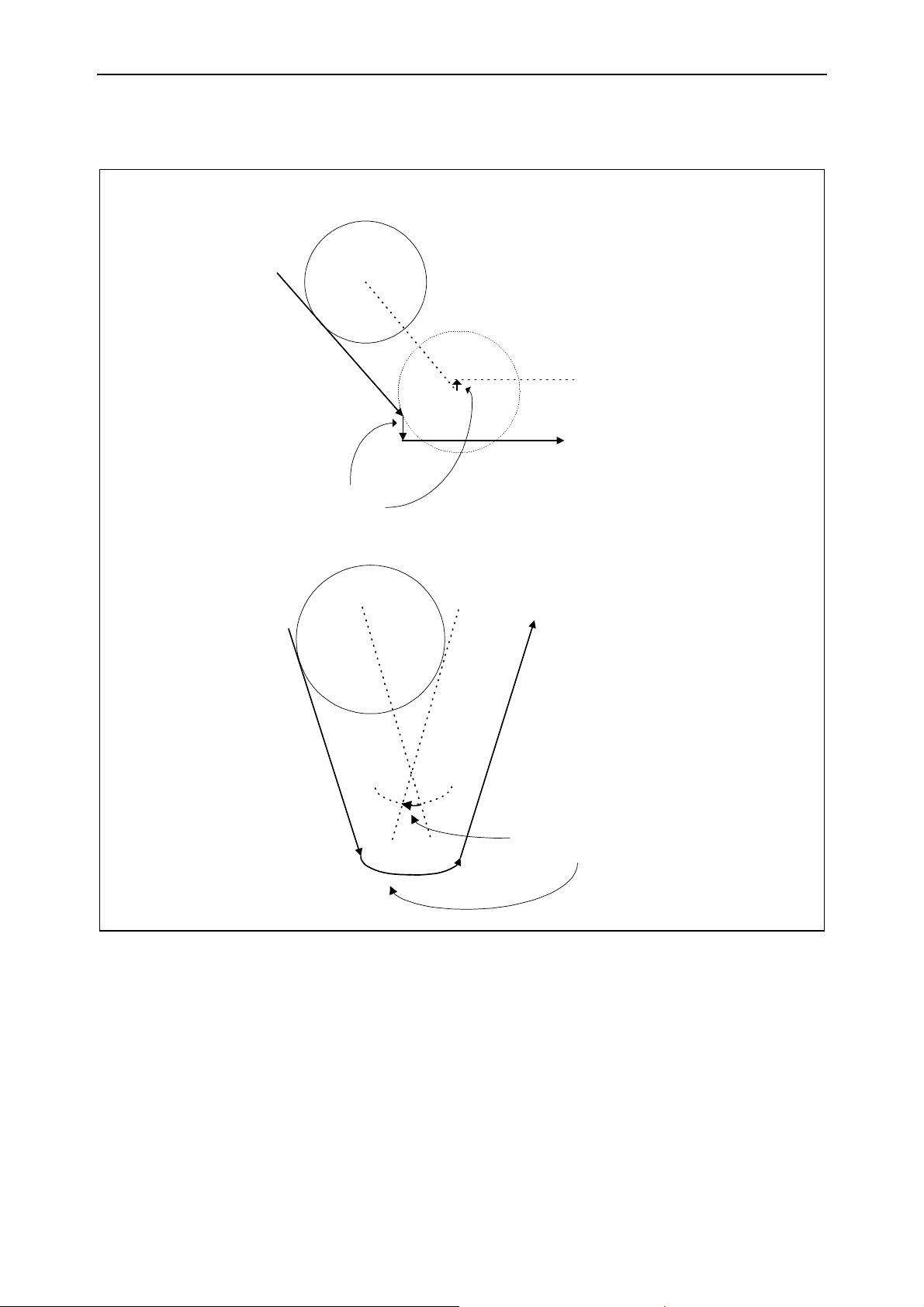
Standard Programming DP

For example, the following types of interference are recognised:

Tool

right

course

programmed

course

Opposite
directions

Example

Tool

right course

programmed

course

Opposite directions

Figure 2.14 - Interference on linear and circular arc paths

G0 G41 X100 Y100 (feed to point P1(X100-tool radius,Y100))
G1 Y200 F500 (linear to point P2(X100-tool radius,Y200))

G2 G40 X200 R50 (arc to point P3(X200+tool radius, Y200))

See also

Tool lenght correction.

END OF CHAPTER

91752.DP.1.GB Esa/Gv2.50

DP Advanced Programming

3 Advanced Programming

3.1 Selecting Automation Language mode

Syntax

Description

See also

MODE = AUTO (default)

This command selects the Esa-Gv Automation Language programming mode, with the
features listed below.
In this mode comments are preceded with a semicolon and the reserved ISO character
"%" is used to identify variable names. For the rest, Automation Language can be
considered an extension of the ISO language.

Standard Programming: Selecting ISO mode

Esa/Gv 91752.DP.1.GB 3.1

Advanced Programming DP

3.2 Parametric Programming

Parametric programming allows variables to be used instead of numeric values or
strings. This makes programming flexible, guaranteeing that the code is clear.

Types of Variables

Three types of variables are available:
ù Global system variables: system or user variables accessible to both the CNC and

operator interface.

ù Pre-defined variables: variables of the numeric type which can be addressed by

means of the Vaxx, VLxx, VGxx codes.

ù Symbolic variables: variables whose names are defined by the user.

3.2.1 Global system variables

Syntax

Description

%nomeregistro
% nomeregistro.numerobit
Global variables defined in the shared memory can be accessed within the system (CNC,
UI, PLC).

To access the registers and structures in the shared memory, the % character must
precede the name of the register in question. If the name of the register is followed by
.numerobit, this means that only one bit is to be tested or modified.
The bit number must be compatible with the size of the register.

Type of register Tolerated range

BYTE from 0 to 7

Example

WORD from 0 to 15
DWORD from 0 to 31

%regtool[0].0=1 ;sets bit 0 of reg. %regtool[0]
%regtool[0].1=0 ;resets bit 1 of reg. %regtool[0]
%regtool[0].2=1 ;sets the bit 2 of reg. %regtool[0]

91752.DP.1.GB Esa/Gv3.2

DP Advanced Programming

3.2.2 Pre-defined numeric variables

These are numeric variables pre-defined by the system. They can be accessed using
codes VA (automatic variables, VL (local variables) or VG (global variables) followed
by the number of the parameter.

All the numerical values in words can be referred to via parameters or expressions, with
the exception of the N codes.
Variables fall into the following categories:

VA xxx Automatic Only visible inside the program or subprogram
VL xxx Local Only visible inside its channel
VG xxx Global Visible to all channels

3.2.3 Assigning a variable pre-defined numeric variables

Syntax

Description

Example

See also

VA, VL, VG number = expression

The variable to the left of the = (assignment) sign is set to the value of the expression on
the right.

G0 X0 Y0 ;Feed to point P1(X0, Y0)
VA1 = 100 VA2 = 200 ;Assigns two variables
G1 F1000 XVA1 YVA2 ;Linear feed to point P2(X100,Y200)

Esa/Gv 91752.DP.1.GB 3.3

Advanced Programming DP

3.2.4 Symbolic variables

The programmer can use personalized variables (the name and type are established by
the user) to which numeric values, strings or references can be assigned. Use of this type
of variable allows the code to be made more comprehensible. To use the symbolic
variables, the machine parameter [System->Configure Channel->Local variables for
Subroutine level] must be different from zero.

Variables of the following Type:

NUMERIC variables that contain both real numbers (numbers with the

decimal point) and integers.
The numbers are expressed in decimals, possibly with decimal

point and sign. Up to 9 whole figures are permitted. The
exponential notation is not permitted.

The expressions are processed in binary mode with a 14-figure

precision.
STRING variables that contain sequences of characters
RECORD variables that enable access to information about another object

which can be a symbolic variable, an input/output register, a user

register defined in defcn, etc.

3.2.5 Declaration of Symbolic Variables

Syntax

Description

DBL symb [=numeric value] [,symb [=numeric value]]
STR symb [= string] [,symb [= string]]
REC symb [= ^value] [,symb [= ^value]]

symb=nomevar[[elem number]]

Before the symbolic variables can be used to compile a PP, they must have been
previously declared.

DBL declares that the following symbols are numeric
STR declares that the following symbols are the string type
REC declares that the symbols are of the record type

The symbolic variables used must be declared at the beginning of the PP.

The name of a symbolic variable:

ù consists of up to 32 alphanumerical characters;
ù cannot correspond to a key word of the programming language;
ù cannot begin with the ‘_ ‘ character.

The variables can be initialized during the declaration phase, i.e. their initial value can
be specified before they are used in the PP. If this value is not specified, the system
assumes a default value, coherent with the type of data item declared.

91752.DP.1.GB Esa/Gv3.4

DP Advanced Programming

Visibility of the
variables

TYPE OF DATA
ITEM

numeric 0.0 zero
string "" empty string
record NULL no reference

Several symbols of the same type can be declared (and initialized if required) on the
same line by separating them with ‘,’ (comma).
Recognition of the variables discriminates between capitals/lower case letters (e.g.
Dimension is not the same as DIMENSION or dimension).

One-dimensional arrays can be declared, for example

DBL QuoteX[10] ; vector of 10 Numeric variables

This allows homogeneous data to be organized so as to enable access by the index.
Since a vector consists of n elements, it cannot be initialized during the declaration
phase.

Personalized variables can be defined within any programming module (main PP,
subroutine and fixed cycles).

The variables defined in the PP or its subroutine are activated and visible until its
conclusion, thus also during execution of a recalled subroutine.

DEFAULT VALUE

Main Pp %1
DBL NRiga ; number of lines to execute
DBL NFORI, MAXY
...
...

NRiga = 20

JSR “boring” Executes a row of holes : boring

N10 .....

IF (NRiga > 20) JMP 10

.....

RET

It is not possible for one or more variables declared on the same subroutine level to have
the same name, while this is allowed for variables defined at different subroutine levels.
The fact of having variables with the same name at different subroutine levels is
resolved in the following way:

ù a variable is always visible within the module in which it is defined;
ù a variable is visible in the modules recalled by the PP/Subroutine if these do not

declare a variable with the same name

Main % 1

DBL AUX1 = 35,
DBL AUX2 = 2

VL0 = AUX2 ; VL0 = 2

JSR 112 -> LEVEL1 : 112

Esa/Gv 91752.DP.1.GB 3.5

Advanced Programming DP

VL2 = AUX2 ; VL2 = 10

VL3 = AUX1 ; VL3 = 35

JSR “SUB1” >LEVEL2 :SUB1

DBL AUX1 = 0

VL4 = AUX2 ; VL4 = 10
VL5 = AUX1 ; VL5 = 0

Example

DBL mezz, MIN=0, QuoteX[10]
REC PUNT[3] ;Array of 3 invalid pointers
REC POINTER = ^mezz
STR SUBROUTINE, NAME[3], SUB=”example.cfu

3.2.6 Allocation of Symbolic Variables

Syntax

Allocation of variables
of the record type

symb = compatible value
symb = nomevar[[elem number]]

Following an allocation, the variable of the record type to the left of the allocation
symbol (=) contains the reference to the allocated symbol. Once a record variable has
been allocated, it can be used instead of the symbol to which it refers.
A variable of the record type can be allocated to another variable of the record type.

REC PUNT[10]
DBL Port, Limit switch

PUNT[0] = ^%C23 ;PUNT[0] is able to access

;logic register C23

PUNT[0] = 15.2 equals %C23=15.2

PUNT[1] = ^%QW3.1 ;PUNT[1] is able to access

; bit 1 of output register QW3

PUNT[2] = ^%IW8 ;PUNT[2] is able to access

;input register IW8

PUNT[3] = ^%subroutine[0].name

;PUNT[3] is able to access the
;structure in defcn subroutine[0].name

PUNT[4] = ^Port ;PUNT[4] is able to access the

;variable of the numeric type Port

PUNT[5] = ^VA20 ;PUNT[5] is able to access the

;pre-defined variable VA20

PUNT[6] = ^VG2;PUNT[5] is able to access the

;pre-defined variable VG2

PUNT[7] = ^VL13 ;PUNT[5] is able to access the

;pre-defined variable VL13

Use of record variables can be useful when variables in the shared memory must be
accessed frequently, as it speeds up the process.

91752.DP.1.GB Esa/Gv3.6

DP Advanced Programming

Allocation of variables
of the numeric type

Allocation of variables
of the string type

The contents of the variable on the left of the allocation symbol (=) is set at the value of
the expression on the right.
Besides being allocated to a defined variable of the DBL type, a numeric value can also
be allocated to a record variable that refers to a symbol of the numeric type.

DBL QuotaX
REC PUNT

QuotaX = 100 ; QuotaX 100.0

PUNT = ^ QuotaX
PUNT = 300 ; equals QuotaX 300.0

The contents of the variable on the left of the allocation symbol (=) is set at the value of
the string on the right.
Besides being allocated to a defined variable of the STR type, a string value can also be
allocated to a record variable that refers to a symbol of the string type.

STR SUB= “fora100.cfu”
REC PUNT

SUB = “1098.cfu” ; SUB “1098.cfu”

PUNT = ^ SUB
PUNT = “boring.cfu” ; equals SUB “boring.cfu”

3.2.7 Expressions

Expressions are created by combining operands and operators as in algebra.
Expressions can be used:

ù To assign the resulting value to a variable, the expression appears on the right of the

“=” sign that follows the variable to which the calculation is allocated.

E.g. MyVar = (VarA ** VarB) * SIN(VarC)/COS(VarD)
ù As condition of an IF instruction; the expression is resolved and the result evaluated

by the IF instruction.

Eg. IF( ( (VarA ** VarB) * SIN(VarC)/COS(VarD) ) > 0 ) THEN

• In line with any ISO instruction.

Eg. GO X(VarA ** VarB) Y(SIN(VarC)/COS(VarD) )
M(VarA-VarB)

Esa/Gv 91752.DP.1.GB 3.7

Advanced Programming DP

Type of operand Syntax

constant number
pre-defined variable VA, VL, VG number
symbolic variable symbol
0x<number> Hexadecimal constant
%C <register number> I/O logic registers
%IW <register number> physical Input registers
%OW <register number> physical Output registers
glob. symbolic vector elem. %name_lowercase_var[el.num.]
global system var. %name_ lowercase_var
Structured glob. system var. %name_ lowercase_var.member
synchronous global system var. ?%name_ lowercase_var

operator

addition (+) expression+expression
subtraction (-) expression-expression
multiplication (*) expression*expression
division (/) expression/expression
negation (-) -expression
Raising expression ** expression

Function Syntax

square root SQRT(expression)
sine
cosine
tangent
arc sine
arc cosine
arc tangent
absolute value
rounding off
truncation
rounding off to the highest figure
addition (for dword)
subtraction (for dword)
multiplication (for dword)

91752.DP.1.GB Esa/Gv3.8

DP Advanced Programming

Boolean operatorrs Description

<espress> AND <espress> and bit to bit operation
<espress> & <espress> and bit to bit operation
<espress> OR <espress> and bit to bit operation
<espress> | <espress> and bit to bit operation
<espress> && <espress> and logic operation (on entire word)
<espress> || <espress> operazton or logica ((on entire word)
SHR(<espress1>, <espress2>) shift right espress1 di espress2 bits
SHL(<espress1>, <espress2>) shift left espress1 di espress2 bits
MOD(<espress1>, <espress2>) resto divisione espress1 modulo espress2

Description

Example

Expressions are composed of constants and variables combined by the listed operators
and functions.
Operators are executed with algebraic priority, with optional parentheses to force
priority ( ).

Numbers are expressed in floating point signed decimal arithmetic with up to 9
significant figures; exponential notation is not allowed.

Expressions are evaluated in 14-bit arithmetic; note that approximates numbers with
significant figures after the decimal point and hence a certain margin of error applies.

Note also that the number of a variable can itself be an expression, thus enabling
indexed variable reference.

VA1 = 2
VA2 = 2000.0
VA3 = VA[VA1] ;indexed variable reference
VA4 = 45.0
VA5 = VA2 + (VA3 * SIN(VA4)) * VA2
G01 F1000 XVA2 YVA5
VA1 = VA1 + 1

N100 %regasync[0] = %nc[1].du[0]
N200 %regasync[1] = %nc[1].du[1]

N600 VA[0] = 1
N600 VL[0] = 2
N600 VG[0] = 3

N900?%regtool[0] = 4.1 * 2 - 1
N900?%regtool[0] = 1
N900?%regtool[0] = 1

N900 %regtool[0].0 = 1
N900 %regtool[0].1 = 0
N900 %regtool[0].2 = 1

N1000?VA[0] = 123.0 * -1
N1000?VA[1] = 123.0 * -2

Esa/Gv 91752.DP.1.GB 3.9

Advanced Programming DP

N1020 VA0 = %regtool[0]

where shared memory is named as follows:

dword regasync[10]

dword regtool[10]

typedef struct{

RETAIN dword du[10];

} DU;

DU nc[5];

Addition

Syntax

Subtraction

Syntax

Negation

Syntax

Multiplication

Syntax

Calculates the algebraic sum of two operands.

exp1 + exp2

Calculates the difference between two operands.

exp1 - exp2

Changes the sign of an operand: an operand with a negative value becomes positive and
vice versa.

- exp1

Calculates the product of two operands.

exp1 * exp2

Division

Syntax

Modulus of the
division

Syntax

Calculates the ratio between two operands.

exp1 / exp2
The value of the dividend (exp2 in the example) must be different from 0.

Calculates the remainder of a division.

MOD(exp1,exp2)
Example:

VAR1 = MOD(5,2)

The result of this division is 2 and the remainder is 1; thus variable VAR1 equals 1.

91752.DP.1.GB Esa/Gv3.10

DP Advanced Programming

Raising

Syntax

Square root

Syntax

Absolute value

Syntax

Rounding off to the
lower integer

Calculates raising of base A with exponent B;

A ** B
This operator has certain limits as to the values it can use:

ù Generates a domain error if A and B are both 0.
ù Generates a domain error if A<0 and B is not an integer.

calculates the square root of the associated value.

SQRT(expr)
The expr value must not be negative.

Calculates the absolute value of the associated operand, i.e. if the value of the operand is
positive it remains unchanged, otherwise it is made positive.

ABS(expr)

Approximates a non-integer value to the lower integer value nearest to the original
value.

Syntax

Rounding off to the
higher integer

Syntax

Trigonometric
operators

FIX(expr)
Example:

VARA = FIX(3.123)

The result of the operation is 3.

Approximates a non-integer value to the higher integer value nearest to the original
value.

FUP(expr)
Example:

VARA = FUP(3.123)

The result of the operation is 4.

The operators listed below use variables or constants that express angles or that provide
an angle as a result, as operands.
The numeric characteristic of the angles is that their value is periodic, i.e. values beyond
the –360° to +360° range can be brought within this range. The operation that brings the
value of an angle back within the illustrated range is called angle normalizing.

Angle normalizing is obtained by applying the 360° modulus function to the angle to
normalize.

Esa/Gv 91752.DP.1.GB 3.11

Advanced Programming DP

Syntax

Arc-Cosine

Syntax

Arc-Sine

Syntax

Arc-Tangent

ALPHA = MOD(BETA,360)
Normalizes the value of the angle in the BETA variable and sets the result in the
ALPHA variable.
Normalizing is implicit and must not be calculated, i.e. the SIN(420) and SIN(60)
functions are equivalent.
All the parameters are given in degrees.

Calculates the arc-cosine of the associated value.
This is the inverse function of the cosine. The value of the parameter must be between –
1 and 1.

ACOS(expr)
The value calculated is an angle.

Calculates the arc-sine of the associated value.
This is the inverse function of the sine. The value of the parameter must be between –1
and 1.

ASIN(expr)
The value calculated is an angle.

Calculates the arc-tangent of the associated value.
This is the inverse function of the tangent. The value of the parameter must be between

-∞ and +∞.

Syntax

Cosine

Syntax

Sine

Syntax

Tangent

Syntax

Logic operators
(Boolean)

ATAN(expr)
The value calculated is an angle.

Calculates the cosine of the associated value.

COS(expr)
Expr is an angle and the value calculated is between -1 and 1.

Calculates the sine of the associated value.

SIN(expr)
Expr is an angle and the value calculated is between -1 and 1.

Calculates the tangent of the associated value.

TAN(expr)
Expr is an angle and the value calculated is between -∞ and +∞..

The characteristic of the logic operators is that they only evaluate two values of a
variable.
The values considered are Boolean values, TRUE or FALSE.

91752.DP.1.GB Esa/Gv3.12

DP Advanced Programming

The TRUE value is associated with a variable if its content is not zero. The FALSE
value is associated if its content is zero.
The result of a comparison always gives a Boolean result, TRUE or FALSE.

Compares if equal

Syntax

Compares if more or
equal

Syntax

Compares if more

Syntax

This operator is significant if used in an expression within a conditioned jump
instruction (IF).
Compares the two operands are gives TRUE if they are equal or FALSE if they are not
equal.

expr1 == expr2

IF( expr1 == expr2 ) JMP .....

This operator is significant if used in an expression within a conditioned jump
instruction (IF).
Compares two operands and gives TRUE if the first is the same or more than the second,
or FALSE if it is less.

expr1 >= expr2

IF( expr1 >= expr2 ) JMP .....

This operator is significant if used in an expression within a conditioned jump
instruction (IF).
Compares two operands and gives TRUE if the first is more than the second, or FALSE
if it is less or if the two are equal.

expr1 > expr2

IF( expr1 > expr2 ) JMP .....

Compares if different

Syntax

Compares if less or
equal

Syntax

Compares if less

This operator is significant if used in an expression within a conditioned jump
instruction (IF).
Compares the two operands are gives TRUE if they are different or FALSE if they are
equal.

expr1 != expr2

IF( expr1 != expr2 )JMP .....

This operator is significant if used in an expression within a conditioned jump
instruction (IF).
Compares two operands and gives TRUE if the first is the same or less than the second,
or FALSE if it is more.

expr1 <= expr2

IF( expr1 <= expr1 ) JMP .....

This operator is significant if used in an expression within a conditioned jump
instruction (IF).
Compares two operands and gives TRUE if the first is less than the second, or FALSE if
it is more or if the two are equal.

Esa/Gv 91752.DP.1.GB 3.13

Advanced Programming DP

Syntax

And

Syntax

expr1 < expr2

IF( expr1 < expr1 ) JMP .....

Allows several logic expressions to be compiled, thus complex test conditions can be
expressed in the conditioned jump.
The AND operator gives TRUE if both the operators it associates are TRUE. It gives
FALSE in all other conditions.

Expr1 && Expr2

The following table outlines the results that can be obtained by applying the AND
operator.

A B Expr1 && Expr2

TRUE TRUE TRUE

TRUE FALSE FALSE
FALSE TRUE FALSE
FALSE FALSE FALSE

A conditioned jump instruction with 2 conditions associated with an AND operator is
illustrated below.

Or

Syntax

IF (Var1 > Var2) && (Var3 < Var4) JMP .....

Allows several logic expressions to be compiled, thus complex test conditions can be
expressed in the conditioned jump.
The OR operator gives TRUE if at least one of the operators it associates is TRUE. Only
if both are FALSE will the OR operator give FALSE.

expr1 || expr2

The following table outlines the results that can be obtained by applying the OR
operator.

Expr1 Expr2 Expr1 || Expr2

TRUE TRUE TRUE

TRUE FALSE TRUE
FALSE TRUE TRUE
FALSE FALSE FALSE

A conditioned jump instruction with 2 conditions associated with an OR operator is
illustrated below.

IF (Var1 > Var2) || (Var3 < Var4) JMP .....

91752.DP.1.GB Esa/Gv3.14

DP Advanced Programming

Negation

Syntax

3.2.8 Use of #QNAN

The logic value of an expression is varied by means of this operator.
The operator does not give TRUE if the operand to which it is associated is FALSE and
gives FALSE if the operand is TRUE.

! expr1

The following table outlines the results that can be obtained by applying the NOT
operator.

Expr1 ! Expr1

TRUE FALSE
FALSE TRUE

A conditioned jump instruction with 1 NOT condition is illustrated below.

IF NOT (A = B) GOTO .....

#QNAN (Quiet Not A Number) is a particular configuration a variable can assume to
indicate that no tolerated numeric value is present. For example, #QNAN will be found
in fixed cycle parameters that have not been explicitly programmed and for which a
default value is not available. Since the ISO language does not allocate an address if
this contains a #QNAN, instructions that move a set of axes that depend on the
combination of programmed parameters without having to check all the combinations
one by one, can be programmed within the fixed cycles, for; e.g. if in the following line
within a fixed cycle:

G0 XVA1 YVA2

...VA1 and VA2 are parameters, this line will only be automatically interpreted as above
if both the values have been explicitly programmed, or:

G0 XVA1

or:

G0 YVA2

...depending on whether only the first variable or only the second variable are present,
and so forth.
If a #QNAN variable is subjected to operations, they will always give #QNAN as a
result.
Boolean comparisons between variables of which at least one is a #QNAN, give
unforeseeable results. This is why comparing a number with #QNAN cannot be done
with something of the IF type ( a == QNAN() )!!! Use the ISQNAN(n) for this purpose,
e.g.:

IF (ISQNAN( VA2 )) ...

To create a #QNAN use QNAN().

Esa/Gv 91752.DP.1.GB 3.15

Advanced Programming DP

3.3 Program flow control

3.3.1 Unconditional jump

Syntax

Description

Example

JMP number
JMP label

JMPF number
JMPF label

Allows modification of the program execution sequence by directing execution to the
block identified by 'number’ . or from the label, Labels are identified by
.alphanumerical string.
Use of the JMPF instruction instead of JMP speeds up the cycle. JMPF only tolerates
jumps to lines that follow the current line, i.e. it only tolerates jumps forward.

N100 ;error signal
N110 G04 F1 ;wait
N120 JMP 110 ;infinite loop
dX=0
.LOOP
G0 X(100+dX) Y(210+dX)
dX = dX + 0.5
IF (dX < 10 ) JMP .LOOP

See also

3.3.2 Test

Syntax

Description

Test, Standard programming: Block number

IF (expression = = expression) <functions> ;equal
IF (expression != expression) <functions> ;not equal
IF (expression > expression) <functions> ;greater than
IF (expression < expression) <functions> ;less than
IF (expression > = expression) <functions> ;greater than or equal to
IF (expression < = expression) <functions> ;less than or equal to
IF (!expression) <functions> ;equal to zero
IF (expression) <functions> ;not equal to zero

Compares two expressions and executes the rest of the block if the logical function
returns true.
N.B.: comparison must be done between commensurable expressions (sign, dimension).
In other words a 16-bit signed word (for example a %QW) cannot be compared to an
unsigned word (for example 0xFFFF written explicitly). To make the comparison the
signed variable must be cast as follows:

91752.DP.1.GB Esa/Gv3.16

DP Advanced Programming

;IF(%QW2 == 0xFFFF) JMP 110 incorrect!!!

IF((%QW2 & 0xFFFF) == 0xFFFF) JMP 110 ; correct

Example

N100 VA1 = 100.0 ;initialise variable
N200 G0 XVA1 ;position X
N300 M80 ;execute machining sequence
N400 VA1 = VA1 + 10.0 ;increment variable
N500 IF (VA1 < 205.0) JMP 200 ;repeat 10 times, then
continue

IF(%C2.1==1) JMP 100
IF((%C2 && %C3 && %C4) || %C2.1 || %C2) JMP 110

IF(%IW1 > 100) JMP 10
; IF(%QW2 == 0xFFFF) JMP 10 incorrect!!!
IF((%QW2 & 0xFFFF) == 0xFFFF) JMP 10 ; correct
IF(%QW2 == 0x1B) JMP 10
IF(%QW2 == %cnerr.err) JMP 10
IF(%QW2.15) JMP 10
IF(%C2.1 == 1) JMP 10

See also

Conditioned Test

3.3.3 Conditioned Test

Syntax

Description

Example

IF condition THEN

ELSE

ENDIF

Checks the condition. If this is true, the following instruction block will be executed
(block 1 of the syntax). If the condition is false, the instruction block that follows the
ELSE key will be executed (block 2 of the syntax, if present). The process joins up after
the key word ENDIF.
A block of instructions within an IF-THEN-ELSE can contain other IF-THEN-ELSE
instructions. The maximum nesting level is 5.

IF( MyVar > 100 ) THEN

ELSE

ENDIF

Block 1

Block 2

G0 X100 Y 100
G4 F2
M19 S45
MyVar = 0

MyVar = MyVar + 1
G0 Z0

Also see

Esa/Gv 91752.DP.1.GB 3.17

Test

Advanced Programming DP

3.3.4 WHILE Block

Syntax

Description

Example

WHILE (condition)

Block

ENDW

Executes the block of instructions for as long as the expression remains true. As soon as
the condition becomes false, the controls passes on to the block that follows ENDW.
If the condition is false at the first iteration, the block will not even be executed once.

WHILE( MyVar != 100 )

G0 X100 Y 100
G4 F2
M19 S45
MyVar = MyVar+1

ENDW

Since this block of instructions is evaluated by a pre-processing stage carried out before
accomplishment of the machine movement in real time, it is advisable to use conditions
that cannot vary in real time. This construction is used to create parametric iterations but
not to block the processing phase until an event occurs (e.g. activation of an input
signal). The following example is not an example of good programming.

Example of improper
use

G0 X100 Y100
WHILE( “%IW0.0” == 0 )

G4 F1

ENDW

This example shows how a physical input is tested in the pre-processing phase. The
previous instruction will be executed as soon as the real-time executor examines it. The
WHILE block therefore has time to reiterate several times before the G0 block is
executed, waiting for the event to occur. Every time the WHILE cycle is reiterated, the
process prepares a G4 instruction to send to the executor block, while the pre-processing
block continues to iterate without a pause, waiting for the end of iteration event.

One of the ways to synchronize the pre-processing block with the executor is to use a
SYN instruction.

G0 X100 Y100
WHILE( “%IW0.0” == 0 )

SYN

G4 F1

ENDW

This method blocks the pre-processing stage until the execution stage has accomplished
each instruction. In the example, this means waiting for the G0 block to have terminated
before executing block G4. In the successive iterations, a new G4 block will only be sent

91752.DP.1.GB Esa/Gv3.18

DP Advanced Programming

to the executor when this has finished with the previous one. In actual fact, a time setting
is included in the pre-processing block.

Also see

3.3.5 REPEAT Block

Syntax

Description

Example

REPEAT, FOR, BREAK

REPET

Block

UNTIL (condition)

Executes the block of instructions for as long as the expression remains false. As soon as
the condition becomes true, the controls passes on to the block that follows UNTIL.
This construction guarantees execution of the block of instructions it contains at least
once. In actual fact, the block is first executed and its condition is only evaluated
afterwards. If the condition is true, the block will not be reiterated. Vice versa, it will be
executed again until the escape condition occurs.

REPEAT

G0 X100 Y 100
G4 F2
M19 S45
MyVar = MyVar+1

UNTIL ( MyVar == 100 )

Example of improper
use

Since this block of instructions is evaluated by a pre-processing stage carried out before
accomplishment of the machine movement in real time, it is advisable to use conditions
that cannot vary in real time. This construction is used to create parametric iterations but
not to block the processing phase until an event occurs (e.g. activation of an input
signal). The following example is not an example of good programming.

G0 X100 Y100
REPEAT)

G4 F1

UNTIL ( “%IW0.0” != 0 )

This example shows how a physical input is tested in the pre-processing phase. The
previous instruction will be executed as soon as the real-time executor examines it. The
WHILE block therefore has time to reiterate several times before the G0 block is
executed, waiting for the event to occur. Every time the WHILE cycle is reiterated, the
process prepares a G4 instruction to send to the executor block, while the pre-processing
block continues to iterate without a pause, waiting for the end of iteration event.

One of the ways to synchronize the pre-processing block with the executor is to use a
SYN instruction.

Esa/Gv 91752.DP.1.GB 3.19

Advanced Programming DP

G0 X100 Y100
REPEAT

SYN

G4 F1

UNTIL ( “%IW0.0” != 0 )

This method blocks the pre-processing stage until the execution stage has accomplished
each instruction. In the example, this means waiting for the G0 block to have terminated
before executing block G4. In the successive iterations, a new G4 block will only be sent
to the executor when this has finished with the previous one. In actual fact, a time setting
is included in the pre-processing block.

See also

3.3.6 FOR Block

Syntax

Description

Example

WHILE, FOR, BREAK

FOR index=start TO end BY step

Block

ENDFOR

Where:

index is the name of the variable that uses the number of iterations as a counter
start is the initial value of the counter
end is the final value of the counter, i.e. the condition that determines the end of the

iteration

step this is the increase applied to the counter on each iteration. It can also have

decimal and/or negative values. In this case, start must be greater than end.

Repeats the block of instructions for the number of iterations required to bring the index
variable from the start value to the end value, increasing it on each iteration of the step
value.
If the “BY step” part is omitted, the process assumes that the increase is unitary.

The following example accomplished 25 iterations (from 0 to 100 at step 2.5)

DBL ind;

FOR ind=0 TO 100 BY 2,5

G0 X100+(ind*2) Y(ind/2)
G1 X(ind/2) Y100+(ind*2)
G4 F (ind/10)

ENDFOR

The following example is identical to the previous one but uses a unitary increase, thus
makes 100 iterations.

DBL ind;

FOR ind=0 TO 100 BY 2,5

G0 X100+(ind*2) Y(ind/2)
G1 X(ind/2) Y100+(ind*2)
G4 F (ind/10)

ENDFOR

91752.DP.1.GB Esa/Gv3.20

DP Advanced Programming

See also

WHILE, REPEAT, BREAK

3.3.7 Cycle interruption - BREAK

Syntax

Description

Example

BREAK

Interrupts any iteration cycle, bringing the execution to the first instruction that follows
the iteration cycle that contains BREAK.
Interruption of a nested iteration cycle with one or more iteration cycles will not stop the
iteration of the outermost cycles.
The BREAK instruction can be used for FOR, WHILE and REPEAT cycles.

DBL ind;
FOR ind=0 TO 100 BY 2,5

G0 X100+(ind*2) Y(ind/2)
G1 X(ind/2) Y100+(ind*2)

IF( %C0.0 == 1 ) BREAK

G4 F (ind/10)

ENDFOR

See also

WHILE, REPEAT, FOR

Esa/Gv 91752.DP.1.GB 3.21

Advanced Programming DP

3.3.8 Repeat

Syntax

Description

Example

RPT start block, end block, number of repeats

Allows repetition of a specified block sequence for the specified number of repeats .
The sequence of blocks to repeat is defined by the start block and end block.
Start and end blocks can be identified by:

ù numeric constant;
ù expression
ù label.

Number of repeats. Can be specified by an expression
Up to 3 levels of nesting are allowed.

G0 X0 Y0 Z200
G0 B0 ;position table at 0°
RPT 10, 70, 1 ;repeat N10-N70 once
10, 70, 1 ;repeat N10-N70 once
G0 B45 ;position table at 45°
RPT G0 B90 B45 ;position table at 90°
RPT 10, 70, 1 ;repeat N10-N70 once

;(Definition of technical parameters for drilling)
N10 T1 M6
N20 G81 DR125 DE100 DH125 FW150 FR15000
N30 X10 Y10 ;drilling
N40 G80 ;cancel G81 mode
N50 T1 M6
;(Definition of technical parameters for tapping)
N60 G84 DR125 DE100 DH125 RW150 RR15000
N70 RPT 30, 30, 1 ;executes tapping

;at the same position where
;drilling has been done

N100 M30

See also

See use with Fixed system cycles and macro instructions

91752.DP.1.GB Esa/Gv3.22

DP Advanced Programming

3.3.9 Nesting levels: sub-programs and fixed cycles

Nesting levels: sub­programs and fixed
cycles

Compilation of a program can be made modular by using the calls to fixed cycles or
subroutines (sub-programs). Besides making the code more legible, this type of
programming enables already written code parts to be reused. A sub-program can recall
another sub-program through to a maximum of 5 nested calls.

Principal %2

sub 1 : 1

sub 2 : 2

level n

level 2

level1

level 0

Figure 3.1 -

Esa/Gv 91752.DP.1.GB 3.23

Advanced Programming DP

3.3.10 Subprogram start (fixed cycle)

Syntax

Description

prototype: fixed cycle name

where:

prototype = var1,var2, ...

var n =[variable]default value or variable

The start subprogram block (fixed user cycle) contains a comment, the start subprogram
character ":" and the subprogram number (fixed cycle name). User fixed cycles
(filename.cfu) can be freely written by the user.

The following description only regards the system fixed cycles.
The subprogram start block (system fixed cycle) contains the prototype, the subprgram
start character ":" and the subprogram number (fixed cycle name). System fixed cycles
(filename.cfs) are factory set.Each subprogram starts with a start block.

Prototype Variables can be listed in any order. They can have any single-letter

address (so that up to 26 variables (A-Z) are allowed). Contain all the
numerical values, except for T and E, which can be followed by a string in
brackets.
Variables with numerical values are passed to the fixed cycle by automatic
variables of type double VA0 => VA25.

Number
fixed cycle

A unique identifying number which corresponds to the partprogram
number.

A variable declared as self-cancelling in the prototype must be declared between square
brackets, and when called can be:

ù by value => the actual value is passed to the fixed cycle;
ù omitted => if the prototype contains a default value for this variable, the default

value is passed; if no default value is specified in the prototype, Nan is passed (Not
A Number).

If the variable is assigned the value Nan, a special ISO command option can be used:
when an ISO address is followed by Nan, the address is ignored. If a feed command for
a given axis is followed by Nan, for example, the axis is ignored (it can therefore not be
one of the currently available axes as listed in the machine parameters). If a G, M or F
address is followed by Nan, the feed or PLC command or speed setting is not executed
(in the case of feed commands, any following commands with valid addresses are
correctly executed in the active mode). This type of functionality, with Nan values, has
been extended to the following addresses:

G, M, T, D, F, S,
X, Y, Z, U, V, W, A, B, C,
R, I, J, K,
TGR (the three values which follow TGR), SVR, SVL,
CHA (chamfer), RAD (radius),

A modal parameter in the prototype must not be in square brackets and, when called,
can be:

91752.DP.1.GB Esa/Gv3.24

DP Advanced Programming

ù by value => the actual value is passed to the fixed cycle;
ù ommitted => if this is the first call of that fixed cycle at that level of nesting, an

error is returned, if not, then the last evaluated value for that fixed cycle at that level
of nesting is returned.

Note that this mode is maintained only at the given level of nesting.
A prototype must be inserted before the symbol:.

Example

A sample part program follows (at nesting level 0):

N30 F100
N40 G17 G0 X 0 Y 0
N50 G100 B 20.0 E "string" C 30.0 N197
B 60.0 ;modal call of G100
N58 G80 ;cancel modality of G100
N59 JMP 197 ;jump forward two lines
N60 G01 X VL100 Y VL104
N197 M10
N199 M30
N200 END

fixed cycle G100(nesting level 1):

[B] C E [F] 30.0 [G] [N]:100 ;prototype
G1 X VA1 Y VA2 ;uses values 20.0, 30.0 of variables B and C
G1 X VA6 Y VA1 A VA6 ;uses Nan, 30.0, Nan of parameters G,
C, G
CALL MrlChangeTool(3,10) ;call C
VL104 = 33
VL100 = 66
G101 A 10 B 11 C 12
RET

and fixed cycle G101(level of nesting 2):

[A] 10.0 B [C] 25.2:101 ;prototype
G1 X VA0 Z VA1;uses values 10.0, 11.0 of parameters A and
B
RET

See also

Call to subprogram, CFU (User fixed cycle) Advanced Programming.

3.3.11 Subprogram end (fixed cycle)

Syntax

Description

Esa/Gv 91752.DP.1.GB 3.25

RET

Returns execution to the calling program.

Advanced Programming DP

3.3.12 Program end

Syntax

Description

END

Terminates program execution.

3.3.13 Call to subprogram CFU (user fixed cycle)

Syntax

Description

JSR number expression.1 expression.2 ... expression.n
JSR "name" expression.1 expression.2 ... expression-.n
JSR variable expr. 1 expr.2..expr.n

The named subprogram is executed before passing to the next block in the linear
sequence.
The subprogram can be specified by

ù from the number;
ù from the alphanumerical name between inverted commas “”;
ù from the content of a string type of variable (symbolic system variable -%nomesub-

or symbolic variable defined by the user).

Variables can be passed to the subprogram by value; the numerical values of the
variables are located by the subprogram in the automatic registers VA0, VA1, ... VAn,
in the order in which they are defined.
Up to 5 levels of nesting are possible.

Example

See also

Main program:

STR NOMESUB
JSR 1 10.0 VA12 (VA10+VA20)

Drilling subprogram: 1
G0 XVA1 YVA2 ;feed to hole position
G1 ZVA0 F1000 ;execute drilling
G0 Z100 ;retract tool from piece
RET ;return to main program

NOMESUB = “holes”
JSR NOMESUB 10.0 VA12 (VA10+VA20)
JSR "holes" 10.0 VA12 (VA10+VA20)

Drilling subprogram: holes
G0 XVA1 YVA2 ;feed to hole position
G1 ZVA0 F1000 ;execute drilling
G0 Z100 ;extract tool from piece
RET ;return to main program

Subprogram start (fixed cycle), Subprogram end (fixed cycle)

91752.DP.1.GB Esa/Gv3.26

DP Advanced Programming

3.3.14 Subprogram call CFS (system fixed cycle)

Syntax

Type of function

Description

G number var expr var expr ...

where

var: [A, B, ..., Z] variable in the prototype

Modal

The named subprogram is executed before passing to the next block in the linear
sequence.
The number following the G code indicates the subprogram in the user-defined system
directories.
The variables which appear in this block must be among those declared in the fixed
cycle prototype, otherwise an error is returned. Variables not explicitly passed to the
subprogram are assigned their default values (self-cancelling variables) or their previous
values (modal variables).
The variables are accessed by the fixed cycle via the automatic variables VA0..VA26.
VA0 contains the value of variable A, VA1 the value of variable B, etc.
Up to 5 levels of nesting are possible.

After the first call of a fixed cycle only those variables which have changed relative to
the first call need be passed explicitly in successive calls.

Example

See also

Main program:

N30 F100
N40 G17 G0 X 0 Y 0

N50 G100 B 20.0 E "string" C 30.0 N197
B 60.0 ;modal call of G100

N58 G80 ;cancel G100 mode
N59 JMP 197 ;jump forwards two lines
N60 G01 X VL100 Y VL104
N197 M10
N199 M30
N200 END

[B] C E [F] 30.0 [G] [N]:100 ;prototype

Subprogram start (fixed cycle), Subprogram end (fixed cycle), Cancels a fixed
cycle’s mode

Esa/Gv 91752.DP.1.GB 3.27

Advanced Programming DP

3.3.15 Cancels a fixed cycle's mode

Syntax

Description

Example

G80

In the blocks following a fixed cycle call, declaring one or more variables involved in
the fixed cycle causes it to execute.

G80 cancels the fixed cycle mode, that is, it allows execution of successive blocks
without automatically calling the fixed cycle itself

In the same way it is possible to cancel a fixed cycle mode with G0, G1,G2 etc...

Main program:

N30 F100
N40 G17 G0 X 0 Y 0

N50 G100 B 20.0 E "string" C 30.0 N197
B 60.0 ;modal call of G100

N58 G80 ;cancel G100 mode
B 45.0 ;position polar axis B

or
G0 B 45.0 ;position polar axis B

See also

[B] C E [F] 30.0 [G] [N]:100 ;prototype

Subprogram start (fixed cycle), Subprogram end (fixed cycle)

91752.DP.1.GB Esa/Gv3.28

DP Advanced Programming

3.3.16 Call-back function in “C” language

Syntax

Description

Example

See also

CALL <function name> (<var1>, <var2>,...)

<var>=<expression>|^<output variable>

Where:
function name is the name of the function in "C".

The parameters passed to the function are listed between round brackets (max 32
parameters).
The fixed cycle C access the parameters by means of a parameter counter and a list of
the parameters themselves, respectively iArgc and Args. Args specifies the type and
value of each parameter. This information allows checking whether the passed
parameter is type-compatible with the function; the correctness of the call can thus be
checked by the cycle itself.

Finally, it will have access to the ISO channel descriptor and a limited series of
functions .

CALL MrlPtiDrill (3, 10)

Esa/Gv 91752.DP.1.GB 3.29

Advanced Programming DP

3.3.17 Forced escape from the interpreter with error

Syntax

Description

Esempio

ERROR( err_nr )

This instruction stops program execution and displays the error message that depends on
the err_nr value.
It can be used to signal faults that have occurred in the automation part created in ISO
language.
The ERROR only has a direct effect on the channel that is executing the program that
invoked it. Other channels in parallel execution continue their execution unless there is
an intervention from the PLC.
The error code can be from 0 to 9999, even though it is advisable to use values over 768
to prevent conflicts with signals used by the firmware of the CNC.
To customize the message to associate with the error, customize the RunXXX.err file,
where XXX means the three-letters that distinguish the language of the translation (ITA,
GER, FRA, ENG ...). The generated alarm is managed in exactly the same way as the
alarms generated autonomously by the NC.

IF( (VL10 < 1000) AND (VL10 > 0) ) THEN

G0 X VL10

ELSE

ERROR( 800 )

ENDIF

In the example, the field of existence of the VL10 variable before using it for
positioning. A fault is signalled if the variable is beyond the field of existence.

91752.DP.1.GB Esa/Gv3.30

DP Advanced Programming

3.4 Special functions

3.4.1 Await termination

Syntax

Type of function

Description

Example

SYN

Self-cancelling

Halts program calculations until the preceding block has terminated execution.
If this command is not specified, program calculations always run several blocks ahead
of actual execution for higher output.
This command is specified in particular to ensure that the information used in
parameters (e.g. information from axis position sensors or limit switches) are checked in
realtime and not in advance.

N100 G1 G91 X-0.5 Y-0.5 ;approach by one step
SYN ;await axis positioning
IF (VG500 == 0) JMP 100 ;if the limit switch has not been
tripped, approach by a further step

3.4.2 Message display in phase with the executor

Syntax

$ (text)

Type of function

Description

Self-cancelling

Displays the text between brackets in synchrony with execution of the blocks that
precede it.

3.4.3 Memory read/write

Syntax

Description

Example

VA, VL, VG parameter_number = %identifier

[?]%identifier = VA, VL, VG parameter_number

Enables reading and writing to a register in shared memory .
[?] indicates writing synchronous with execution.
Note that the unit of measurement used by the whole value variable is crucial, in the case
of a linear axis position it is a thousandth of a mm (µm), hence, to convert to a floating
point value it must be divided by 1000.

?%MYMEAS = VA11

Esa/Gv 91752.DP.1.GB 3.31

Advanced Programming DP

See also

Enter a physical or logical output

3.4.4 Enter a physical or logical output

Syntax

Description

?%QW <output number> = 1 ;sets the physical output to synchronous mode
?%QW <output number> = 0 ;resets the physical output in synchronous mode
[?]%C <output number> = 1 ;sets the logical output in synchronous or asynchronous
mode
[?]%C <output number> = 0 ;resets the logical output in synchronous or
asynchronous mode

The character '?' indicates that the operation must be executed synchronously with the
other blocks of the program.

?%QW10.4 = 1 ; sets the bit 5 of physical output 10
?%QW10.4=0 ; resets bit 5 of physical output 10
?%QW10=10 ; assigns the value 0x01010 to physical output 10

Writing to physical outputs must be synchronous with execution to ensure the integrity
of the IO states which can also be accessed by the PLC.

?%C10.2 = 1 ; sets bit 3 of logical output 10
?%C10.2 = 0 ; resets bit 3 of logical output 10
?%C10= 14 ; assigns the value 0x01110 to logical output 10

Example

See also

The value of a physical or logical input can be tested with an IF statement.

Writing to physical registers (%QW) must be done synchronously (so that the registers
are not overwritten by the PLC refresh cycle). Writing to logical registers (%C) can also
be asynchronous if the register in question is not used by the PLC.

?%C2.0 = 1
?%C2 = 13
%C2.1 = 0
%C2 = 14
?%QW2.1 = 1

IF(%QW2 > 100) JMP 110
IF(%IW2.1==1) JMP 200
IF(%C2.1==1) JMP 100

IF((%C2 && %C3 && %C4) || %C2.1 || %C2) JMP 120

Reading and writing memory’s register

91752.DP.1.GB Esa/Gv3.32