ElektroPhysik QuintSonic 7 Technical Manual And Operating Instructions

Download

ElektroPhysik

Technical Manual and Operating

Instructions

Ultrasonic Coating

Thickness Measuring System QuintSonic 7

ElektroPhysik

Dr. Steingroever GmbH & Co. KG

Pasteurstr. 15

50735 Köln

Deutschland

Tel.: +49 221 752040

Fax.: +49 221 7520467

Internet: http://www.elektrophysik.com/

Mail: info@elektrophysik.com

Table of Contents

1 Introduction .......................................................................................................................... 8

1.1 General Remarks ............................................................................................................ 8

1.2 Field of Applications ........................................................................................................ 8

1.3 Measuring Procedure ...................................................................................................... 8

1.4 The QuintSonic 7 Measuring System ............................................................................... 9

2 First Steps .......................................................................................................................... 11

2.1 Insert batteries and connect sensor ............................................................................... 11

2.2 Switching-on and taking readings .................................................................................. 12

2.2.1 Setting language .................................................................................................... 13

2.2.2 Taking readings ..................................................................................................... 14

3 Description of the System ................................................................................................. 16

3.1 Display unit .................................................................................................................... 16

3.1.1 General properties ................................................................................................. 16

3.1.2 Operating keys ....................................................................................................... 16

3.1.3 Sockets and Interfaces .......................................................................................... 17

3.1.4 Power Supply......................................................................................................... 18

3.2 Sensor ........................................................................................................................... 19

3.2.1 SIDSP®-Technology ............................................................................................... 19

3.2.2 Measuring ranges .................................................................................................. 21

4 User Interface ..................................................................................................................... 22

4.1 Important Menu Screens ............................................................................................... 22

4.1.1 Start screen ........................................................................................................... 22

4.1.2 Measure mode – numerical and graphical screen .................................................. 23

4.1.3 Measure mode – Large numerical screen .............................................................. 24

4.1.4 Measure Mode – A-screen Image with Echo Signal ............................................... 25

4.1.5 Statistics screen ..................................................................................................... 26

4.1.6 Main menu ............................................................................................................. 27

4.2 How to navigate in the main menu ................................................................................. 28

4.3 Parameter setting .......................................................................................................... 29

4.3.1 Setting a switch parameter (Example: Backlight) ................................................... 29

4.3.2 Setting selection parameters (Example: language) ................................................ 30

4.3.3 Setting a numerical parameter (Example: pos. clip-limit) ........................................ 30

4.3.4 Alphanumercial parameter entries (Example: directory name) ............................... 31

5 Calibration .......................................................................................................................... 33

5.1 Particularities of ultrasonic coating thickness measurement systems ............................ 33

5.2 How to calibrate for the sound velocity .......................................................................... 33

6 Measure Mode .................................................................................................................... 36

Table of Contents

6.1 Important remarks on ultrasonic measurement .............................................................. 36

6.2 Limits to the measurement technique ............................................................................ 37

6.3 Settings to make prior to measurement ................................................................ ......... 39

6.3.1 Using the Direct Mode ........................................................................................... 39

6.3.2 How to create or select a batch .............................................................................. 40

6.3.3 Selecting a measuring range ................................................................................. 40

6.4 How to prepare Measurement ....................................................................................... 41

6.4.1 Taking a reference signal ................................................................ ....................... 41

6.4.2 Selecting a couplant............................................................................................... 42

6.4.3 Checking / carrying out calibration ......................................................................... 43

6.5 Taking Readings............................................................................................................ 44

6.5.1 How to use the sensor ........................................................................................... 44

6.5.2 Measuring procedure ............................................................................................. 45

7 Signification and Use of A-scan Images ................................ .......................................... 47

7.1 Introduction .................................................................................................................... 47

7.2 Description of A-scan Image Types ............................................................................... 48

7.2.1 Reference signal .................................................................................................... 48

7.2.2 Raw measuring signal ............................................................................................ 49

7.2.3 Echo signal with echo lines .................................................................................... 50

7.3 Application ..................................................................................................................... 52

7.3.1 Reference signal .................................................................................................... 52

7.3.2 Raw measuring signal ............................................................................................ 52

7.3.3 Echo signal with echo lines ................................................................................... 52

7.4 How to use the A-scan screen ....................................................................................... 59

7.4.1 Zoom-in and zoom-out in amplitude direction......................................................... 61

7.4.2 Zoom- in and zoom-out in time direction ............................................................... 61

7.4.3 Graphics cursor and displacement in time direction ............................................... 62

7.4.4 Zoom and position indicator ................................................................................... 63

7.4.5 A-scan image menu ............................................................................................... 63

7.4.6 Measure mode with A-scan image being shown .................................................... 65

7.4.7 Icons to identify invalid echoes .............................................................................. 65

7.4.8 Quit the A-scan image ........................................................................................... 66

8 Echo Signal Processing .................................................................................................... 67

8.1 Introduction .................................................................................................................... 67

8.2 Levels of Processing ..................................................................................................... 68

8.3 Preprocessing ............................................................................................................... 68

8.3.1 General remarks .................................................................................................... 68

8.3.2 Time-clipping ......................................................................................................... 69

Table of Contents

8.3.3 Amplitude-clipping ................................................................................................. 69

8.4 Least-Squares Optimisation .......................................................................................... 73

8.5 Postprocessing .............................................................................................................. 74

8.5.1 General remarks .................................................................................................... 74

8.5.2 Multiple-echo suppression ..................................................................................... 74

8.5.3 Manual echo selection ........................................................................................... 75

8.5.4 Blocked domains ................................................................................................... 76

8.5.5 Expectancy domains .............................................................................................. 77

8.5.6 Number criteria ...................................................................................................... 78

9 Tips and tricks ................................................................................................................... 81

9.1 Cross-section ................................................................................................................ 81

9.2 Measuring range............................................................................................................ 81

9.3 How to proceed for a new setting of task ....................................................................... 81

9.4 Amplitude clipping with optimisation enabled ................................................................ . 82

9.5 High level of unwanted echoes in the layers .................................................................. 82

9.6 Inhomogeneous bases .................................................................................................. 83

9.7 Multiple reflections ......................................................................................................... 83

9.8 Measuring object of unidentified nature ......................................................................... 83

9.9 Interaction of preprocessor, optimisation and postprocessor parameters ...................... 84

10 Application examples ........................................................................................................ 86

10.1 Three-layer paint on plastic ........................................................................................... 86

10.2 One-layer paint on wood ................................................................................................ 86

10.3 Two-layer paint on steel ................................................................................................. 87

10.4 Thin one-layer paint on body sheet ................................................................................ 88

10.5 Wall thickness measurement ......................................................................................... 89

10.6 Multi-layer plastics foil ................................................................................................... 89

11 Data Management .............................................................................................................. 91

11.1 Introduction .................................................................................................................... 91

11.1.1 Batches .................................................................................................................. 91

11.1.2 Memory capacity / using the data memory ............................................................. 91

11.1.3 Parameter sets ...................................................................................................... 91

11.2 Data base ................................ ................................................................ ...................... 92

11.2.1 General remarks / How to call the data base.......................................................... 92

11.2.2 Directories ............................................................................................................. 92

11.2.3 Batches .................................................................................................................. 97

11.2.4 Parameter sets .................................................................................................... 104

12 Setting Parameter Sets .................................................................................................... 106

12.1 Edit a parameter set (alphanumerically) ...................................................................... 106

Table of Contents

12.1.1 General ................................................................................................................ 108

12.1.2 Preprocessor ....................................................................................................... 108

12.1.3 Optimisation ......................................................................................................... 110

12.1.4 Postprocessor ...................................................................................................... 111

12.1.5 Edit the User-values table .................................................................................... 118

12.2 Edit a parameter set (graphically) ................................................................................ 120

12.2.1 How to call the menu ........................................................................................... 121

12.2.2 Clipping ................................................................................................................ 121

12.2.3 Blocked domains ................................................................................................. 131

12.2.4 Expectancy domains ............................................................................................ 134

13 Statistics / Batches ................................................................................................ .......... 139

13.1 General remarks .......................................................................................................... 139

13.2 View statistics .............................................................................................................. 139

13.2.1 Statistical values .................................................................................................. 139

13.2.2 Readings ............................................................................................................. 140

13.2.3 Histogram ............................................................................................................ 141

13.2.4 Trend diagram ..................................................................................................... 142

13.2.5 Help / Extras ........................................................................................................ 143

13.3 Delete a reading from a batch ...................................................................................... 143

13.3.1 Delete single readings ......................................................................................... 143

13.3.2 Delete all readings ............................................................................................... 144

13.3.3 Delete a current value .......................................................................................... 144

14 Data Output / Data Transfer ............................................................................................ 145

14.1 Data print-out ............................................................................................................... 145

14.2 Transfer data to a PC (terminal program) .................................................................... 146

14.3 Data transfer to a PC (QSoft 7) .................................................................................... 148

15 The Menu .......................................................................................................................... 149

15.1 Main menu ................................................................................................................... 149

15.2 Submenu “Database“ .................................................................................................. 149

15.3 Submenu “Statistics” ................................................................................................... 149

15.4 Submenu “A-scan image” ............................................................................................ 149

15.5 Submenu “Active batch” .............................................................................................. 150

15.5.1 Properties ............................................................................................................ 150

15.5.2 Readings ............................................................................................................. 150

15.5.3 Configuration ................................................................ ....................................... 151

15.6 Submenu “Setup” ........................................................................................................ 152

15.6.1 General remarks .................................................................................................. 152

15.6.2 Display ................................................................................................................. 152

Table of Contents

15.6.3 Date / time ........................................................................................................... 153

15.6.4 Data output .......................................................................................................... 153

15.6.5 User preferences ................................................................................................. 156

15.6.6 Gauge specifications ............................................................................................ 157

16 Special Functions ............................................................................................................ 158

16.1 Initialisation .................................................................................................................. 158

16.2 Special functions menu................................................................................................ 159

16.3 Sensor service menu ................................................................................................... 160

16.3.1 Call the service menu .......................................................................................... 160

16.3.2 A-scan images for servicing purpose ................................................................... 160

16.3.3 Readjust the magnetic switch .............................................................................. 161

16.3.4 Readjust the sensor tip echo suppression ............................................................ 162

16.3.5 Readjust the temperature compensation reference point ..................................... 162

17 Connectable accessories ................................................................................................ 164

17.1 General remarks .......................................................................................................... 164

17.2 Direct connection ......................................................................................................... 164

17.3 Connection via the multi-purpose connection box ........................................................ 166

18 Care and Maintenance ..................................................................................................... 167

18.1 Care ............................................................................................................................ 167

18.1.1 Using NiMH storage batteries .............................................................................. 167

18.2 Maintenance.................................................................................................................... 167

19 Technical Data ................................................................................................................. 168

19.1 Gauge specifications ................................................................................................... 168

19.2 1 Gauge specifications ................................................................................................ 168

19.3 Sensor ......................................................................................................................... 169

20 Supply Schedule, Accessories ....................................................................................... 171

20.1 Supply schedule .......................................................................................................... 171

20.2 Accessories ................................................................................................................. 172

21 Appendix .......................................................................................................................... 173

21.1 Error messages and trouble shooting .......................................................................... 173

21.2 Statistical Terms .......................................................................................................... 178

21.3 Safety Notes ................................................................................................................ 180

21.4 Declaration of Conformity ................................................................................................ 181

21.4 After-sales Service ...................................................................................................... 182

22 Change-history ................................................................................................................ 183

23 Index ................................................................................................................................. 183

Introduction

1 Introduction

1.1 General Remarks

This instruction manual describes how to use the ultrasonic coating thickness measuring system QuintSonic 7 and provides all necessary information on the manifold application options offered by the system.

Section 2 provides short instructions along with an operating example. All further sections deal with the individual subjects. For technical data and general information on care and maintenance, supply schedule and accessories, please refer to the end of this manual.

1.2 Field of Applications

QuintSonic 7 is an ultrasonic coating thickness measuring system for measuring paint, lacquer and plastic layers applied on metal, plastic, wood, glass or ceramic. Up to five layers can be measured non-destructively in one operation. Thanks to the innovative technology, QuintSonic 7 is the first gauge of its kind to determine exactly the layer thickness applied on components made of GRP or CRP material. QuintSonic 7 offers a wide range of applications in the automotive industry, aerospace or any other industrial branch. Additional feature: QuintSonic 7 can also be used for measuring thin bases through the coating, especially the wall thickness of thin metal sheets starting from 50 µm.

1.3 Measuring Procedure

The working principle of QuintSonic 7 is based on the reflection of ultrasonic waves at the interfaces between the individual layers of a coating system. For measurement, a liquid or pasty couplant is applied on the sample at the point of measurement. The sensor is put on the measuring spot. The high-frequency ultrasonic sound generator of the sensor head emits an ultrasonic pulse of a broad bandwidth to travel through sensor head, couplant and finally through the coating system. At each interface between two layers as well as at the interface to the base, some of the sonic energy reflects. These portions of pulse – also referred to as “echoes” – return to the measuring head at different velocities and the receive signals are registered in the measuring head. As the time of travel is a function on the sound velocity in the respective material, it can be used as indicator for the coating thickness. Thickness is calculated according to the time of travel and sound velocity, transferred to the gauge and shown on display.

Unlike in wall thickness measurement, the layers to be measured with ultrasonic coating thickness gauges are extremely thin and thus travel times very short, i.e. in the nanoseconds range (a

Introduction

billionth of a second). As a consequence, the sound echoes may overlap in the receive signal. Before the signal evaluation can take place, it is necessary to separate the individual echoes with respect to their travel times. This is done in a complex mathematical process. Thanks to the high computing power of the sensor, the complete measuring result is made available not later than after one second approximately.

Some measuring samples such as GRP or CRP materials exhibit material discontinuities (inhomogeneities) or inclusions in the base that may cause false echoes. QuintSonic 7 offers a

wide range of methods for the suppression of unwanted echoes so that only the “true” echoes, i.e.

the sound waves reflected from the layer interfaces, will be used for evaluation.

1.4 The QuintSonic 7 Measuring System

The portable system consists of two elements:

 The intelligent ultrasonic SIDSP®-technology based sensor (see section 3.2.1)  The operating and display unit

Both elements are cable connected. Designed for user-friendly operation, QuintSonic 7 features an intuitive menu control with context-

sensitive online help. Large backlit control keys allow extra comfort. Excellent viewing conditions provided by the large backlit graphics display allow convenient usage at night and in conditions of poor visibility.

Special feature of QuintSonic 7: A-scan images (see section 7) are shown directly on the gauge display for immediate quality assessment of the readings obtained without the need to connect a computer. On the other hand, additional PC software is available (see below) to provide largesized coloured A-scan images on your computer. This makes QuintSonic 7 the ideal tool for both, portable use on site or use in the laboratory.

The advanced PC-like data management offers quick creation of folders and easy set-up of customized batches. QuintSonic 7 simplifies the calibration and parameter set-up allowing to solve also difficult settings of task in a minimum of time without the need for special skills.

The „QSoft7 Basic“ PC software (supplied with the gauge) enables easy parameter setting via the usual input devices (keyboard, mouse) of your computer. In addition, large, colour A-scan images can be displayed on your computer screen.

As an option, the PC software “QSoft 7 Professional” is available, for convenient set up and evaluation of measuring groups and export in various data formats. The software exports data as text documents, Excel® spread sheets or in the PDF file format and allows entries of notes and annotations. Also pictures of your measuring samples may be added to the data reports.

Featuring numerous interfaces, QuintSonic 7 connects to peripheral devices such as the portable printer MiniPrint 7000 (available as an option). The standard supply schedule of the QuintSonic 7 includes an infrared interface (IrDA® 1.0) as well as a USB adapter cable. Via this cable, a USB

Introduction

interface is available. As an option, a multi-purpose adapter unit can be supplied to provide an extra USB interface for connecting a mains unit, headphones, a footswitch and or an alarm device. If only single functions are requested, an RS232 adapter cable as well as an IR/ USB converter unit (for connecting a PC) can be supplied.

First Steps

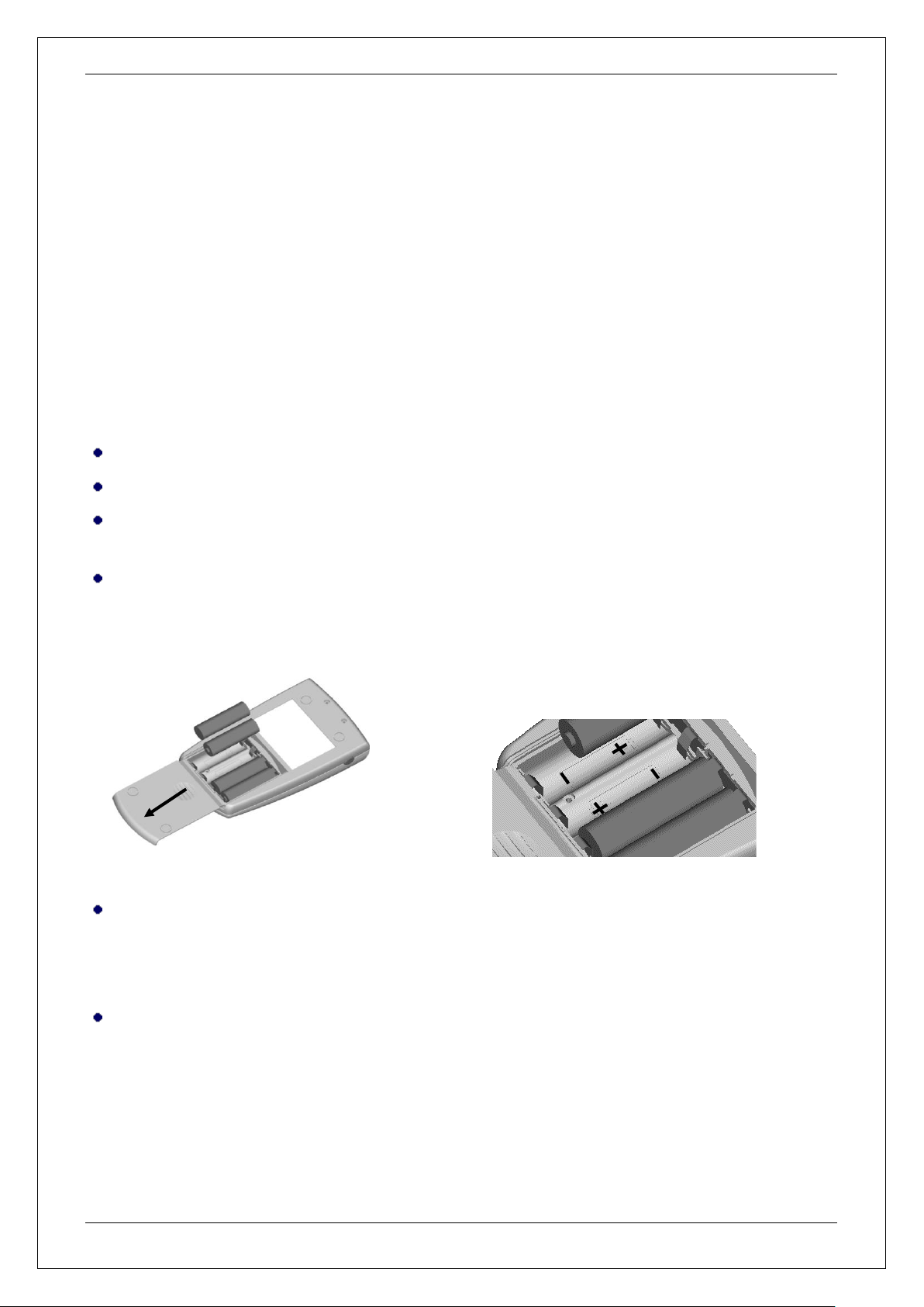
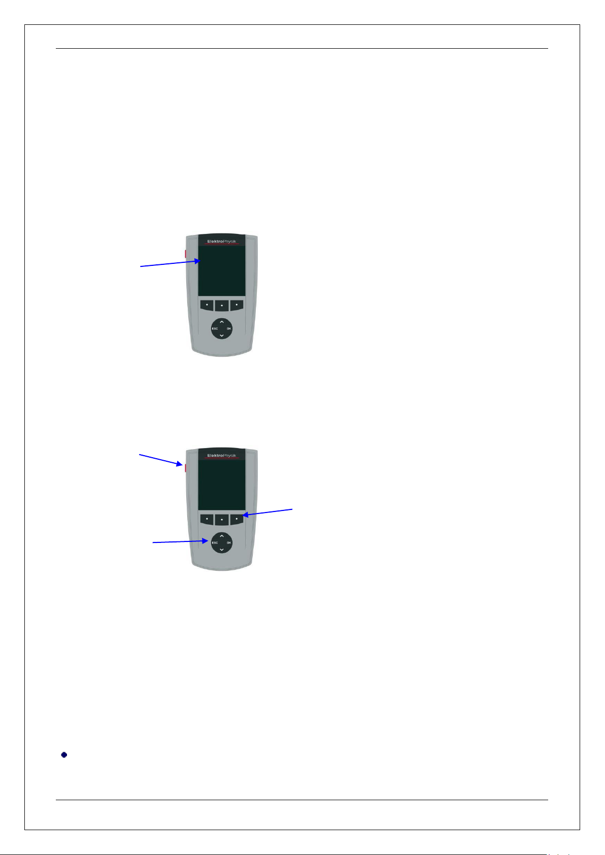
Open the battery compartment

Insert batteries

2 First Steps

This section is addressed to persons to use the gauge for the first time. It explains the main features of the gauge and how to take readings. For a better overview and simplification, this section will not discuss all details. For a detailed description of all subjects please refer to the relevant sections later in this manual.

2.1 Insert batteries and connect sensor

Take gauge and batteries from the carrying case. Push the battery compartment lid in direction of the arrow (as shown below). Insert the batteries supplied with the gauge into the battery compartment. Respect polarities

(as shown below).

Push the battery lid over the housing and close housing.

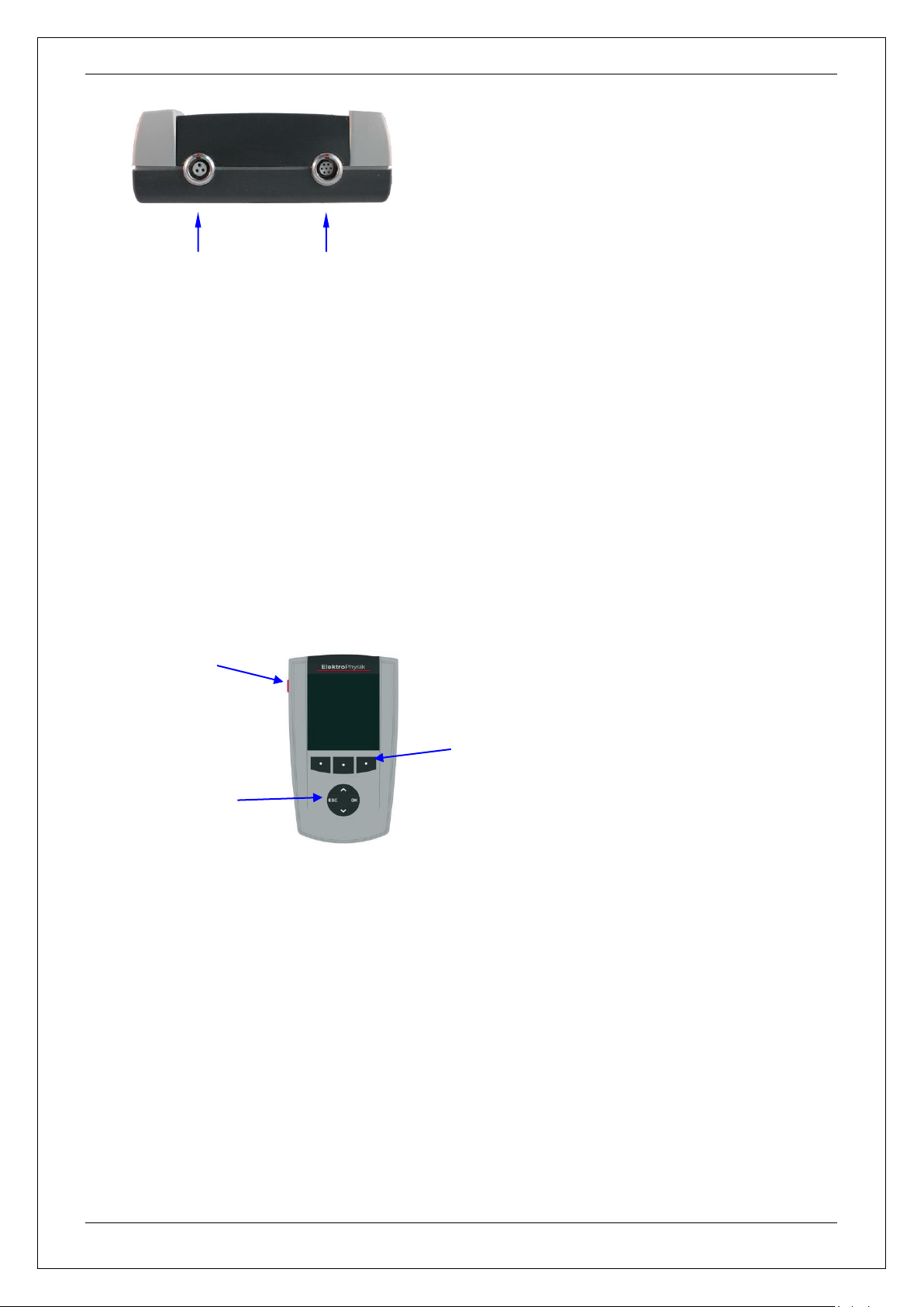
Take the sensor form the carrying case and connect it to the sensor socket on top of the base

unit (see fig. below). Make sure the nib of plug is correctly inserted into the guide way of socket. The red marking at the connector must be positioned correctly to the red marking of the socket.

Fully engage the sensor plug into the sensor socket all the way to the stop.

First Steps

sensor socket

multi-purpose socket

Function keys

ON/OFF-button

Command and navigation block

2.2 Switching-on and taking readings

The gauge is equipped with a round-shaped navigation key block with the following functions: “ESC“, ““ and ““ (arrow up/down). Three functions keys are located below the display. Their current function is shown above the

respective key at the bottom of display. The “ON/OFF“ -button is located on the left side of gauge.

Prior to the initial operation of the gauge, please proceed according the instructions below. The menu will guide you through the procedure.

First Steps

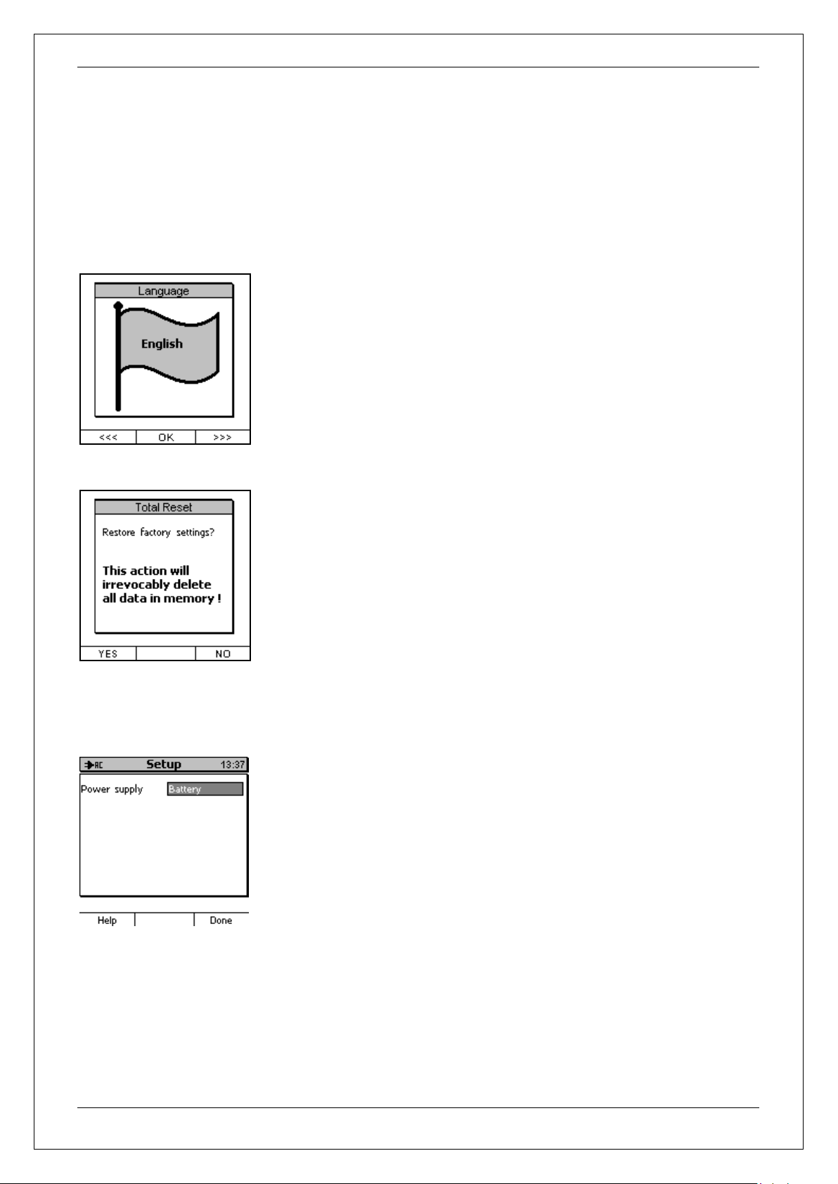
A banner appears with the currently set language. Use arrow arrow up/down-keys to go to the requested language option. Press OK-key or OK-function key to confirm.

Now “Total Reset” appears on display. A Total Reset restores the factory settings. For the initial operation, there is no need to carry out this function.

Therefore press the “NO” function key.

To complete the initialisation procedure, the type of power supply is displayed. Do not change this setting. Just confirm by pressing “Finish” (Done).

2.2.1 Setting language

Press the red ON/OFF button on the left side of gauge and ESC simultaneously. First release ON/OFF key. The initialisation menu will appear.

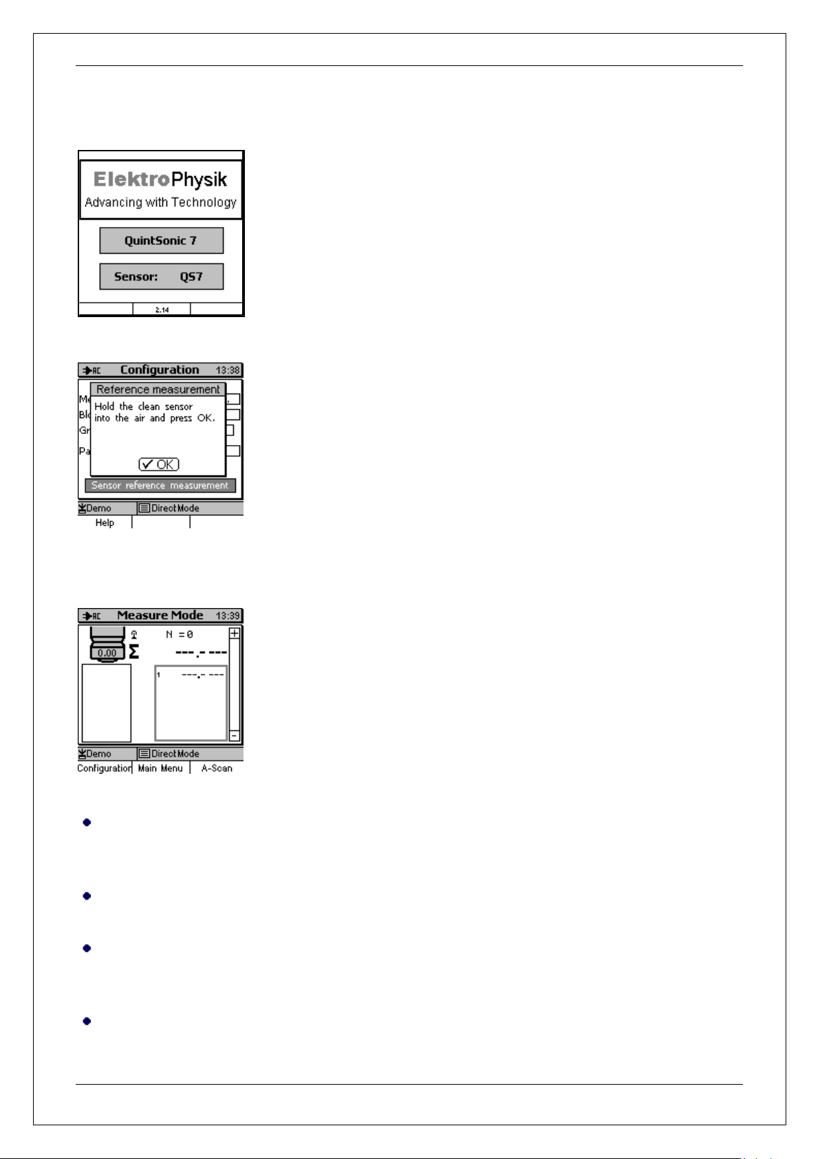
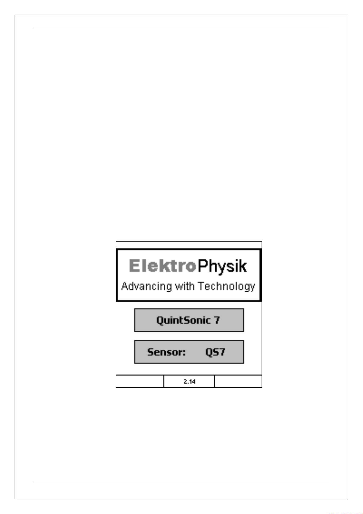
2.2.2 Taking readings

The start screen appears for about 3 seconds showing company logo, gauge version and the type of connected sensor.

You will be requested to hold the sensor into the air for taking a reference signal. Please check the transparent measuring surface of the sensor tip. Make sure it is clean and free of dust, dirt, grease or couplant residuals. If necessary, use a moist soft cloth for cleaning.

Lift the sensor and hold it in the air. Press OK to proceed on acquisition of the reference signal.

Once the signal has been taken, the gauge will switch automatically to measuring mode.

The gauge is ready for measurement and the measuring screen appears. At this point, no reading is available.

First Steps

The "Direct mode“ (see section 6.3.1) along with the parameter set "Demo“ are preset. The

current setting is always shown in the status line. In this setting you can take readings at a medium accuracy. It is not necessary to make further settings prior to measurement.

Take the test foil from the case. Open the bottle with couplant by raising the measure pourer.

Apply a small quantity of couplant on one side of the centre of foil.

Hold the grey spring-loaded sleeve of the sensor with one hand and place the sensor vertically

onto the measuring spot where you have applied the couplant. Push the sensor sleeve fully down to the stop.

Measurement will launch automatically. This will take around one second.

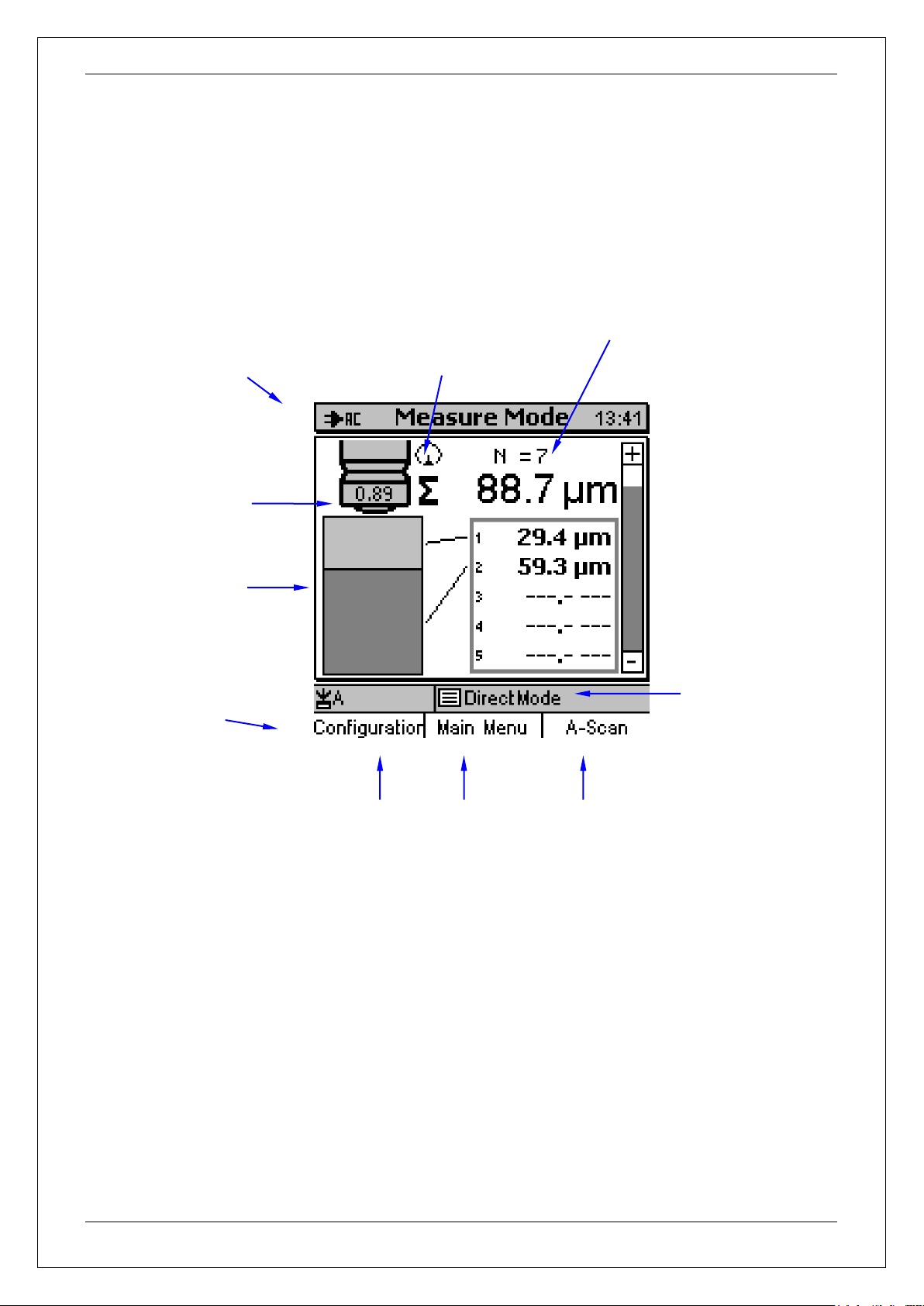
Lift the sensor from the measuring spot. The reading is shown on display (see below).

Schematic representation of the layer system (here: one layer only

Active parameter set (in this figure “Demo“)

Active batch (here: “Direct mode”)

Current properties of the function

keys

Number of readings

stored in the batch

Coupling index

flashing antenna icon

(if sensor is connected)

Time

Total thickness

Thickness #1

Sensor icon

First Steps

Repeat measurement as requested. Make sure a sufficient quantity of couplant is applied on

the measuring surface of the sensor, otherwise no readings will be obtained and an error message appears “Coupling echo faulty !”. If necessary, apply some more couplant.

After measurement has been completed, use a clean cloth to clean the foil and the sensor

measuring surface. Briefly press ON/OFF-button to switch off the gauge.

The figure above shows all data displayed on the measuring screen. For more details please

refer to the following sections of this manual.

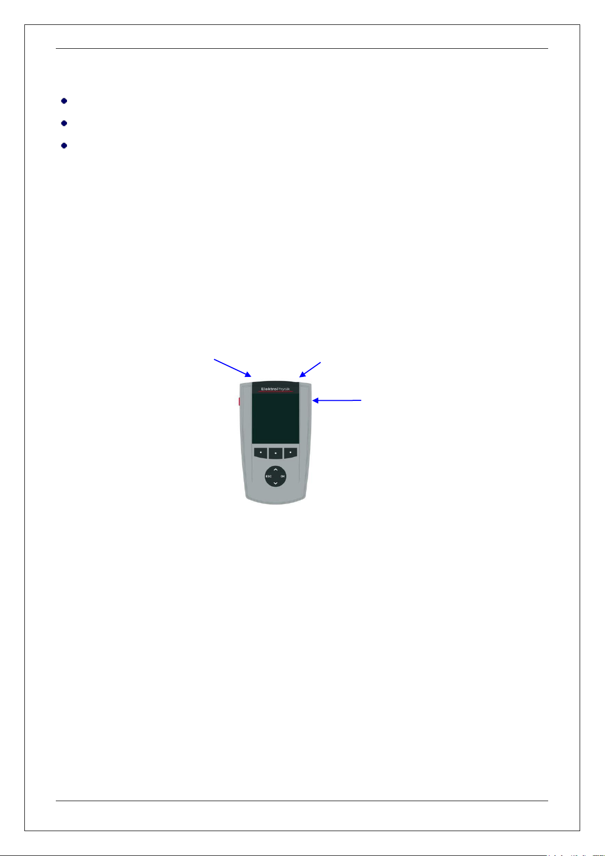
3 Description of the System

Function keys ON/OFF button

Command and navigation key-block

Graphical display 160 x 160 dots

Large backlit display for easy reading of measuring values, A-scan image, statistical data, histogram and trend diagram.

Robust scratch resistant plastics housing.

3.1 Display unit

3.1.1 General properties

Description of the System

3.1.2 Operating keys

Use the ON/OFF button to switch the gauge ON or OFF. If, at switch on, you press ON/OFFbutton and ESC simultaneously, the initialising procedure will be launched (for more details please refer to section 16.1). If you press the ON/OFF-button for a longer time while the gauge is in switched-on state, the Special Functions menu will be called (s. section 16.2).

The Function keys may assume different functions according to the screen content. Their current properties are shown on display upper to the function keys.

The command and navigation key block may also assume different functions:

Press OK to confirm settings, store values or select items from the menu.

Description of the System

Multi-purpose socket

Sensor socket

Infrared interface

Press ESC to abort actions or quit submenus. Use arrow up/down-keys to navigate through the menu or change settings. If the alphanumerical block has been activated, OK and ESC keys will also assume navigation

functions.

In poor-lit conditions, the function keys and the command and navigation key-block may be backlit (see also section 15.6.2).

Most screens dispose of a “Help” Function key for calling the context-oriented on-line “Help“. Press the “Help” Function key on the left to call the direct help.

3.1.3 Sockets and Interfaces

The sensor socket connects to all SIDSP® coating thickness sensors of the MiniTest 7 series, also to sensors such as the F-, N- or FN-type (magnetic induction and/or eddy currents principle), i. e. you only need one display unit and can operate several sensors. The multi-purpose socket is used for connecting the plug-in mains unit or other optional accessories such as the foot switch, the alarm device, RS232 interface cable, USB interface cable, headphones or the multi-purpose connection box (see sections 15.6.4 and 17).

Note: This manual only describes the operation of the QuintSonic 7 as an ultrasonic coating thickness

gauge. If you wish to connect the display unit to an F, N or FN sensor, please refer to the MiniTest 7400 operating instructions.

Description of the System

3.1.4 Power Supply

3.1.4.1 Batteries and storage batteries

The QuintSonic 7 gauge is powered by a set of four alkaline-manganese cells, 1.5V, AA LR6 size, (batteries included in the standard supply schedule). As an alternative, it may be operated on rechargeable NiMH storage batteries (type AA-HR6 or via a plug-in mains unit (available as an option). Please use only products recommended by ElektroPhysik. Please also refer to section 17 “Accessories”.

If you wish to use the storage batteries, they must be recharged using the external charger unit (available as an option). Make sure to adjust the gauge to storage battery operation (see section

16.1). For more details on the use of batteries and storage batteries, please also refer to section 18 “Care and maintenance”.

Important notes:

Remove batteries or storage batteries from the instrument if you are not going to use the gauge

for a longer period of time.

The battery symbol indicates the battery/storage battery state in 6 stages: (0, 20,

40,…100%). If the lowest stage has been reached, “Battery almost empty” will be indicated. In case of total discharge, “Battery too low” will be indicated and the gauge will switch off. Make sure to replace empty batteries within a period of about one minute after you have

removed the exhausted ones. If the gauge remains longer without power, date and time

settings will get lost. If the time interval for battery change has been exceeded, “Check clock

setting” is shown after you have inserted fresh batteries (see also section 15.6.3). Batches and

calibration values, however, are retained in memory. For field use, replacement batteries should be made available. Erratic readings due to low battery voltage do not occur. If voltage is too low, the gauge

switches off or will not switch on at all. Used or defective batteries or storage batteries may contain hazardous substances and must

be disposed according to the legal provisions of your country.

3.1.4.2 Plug-in mains unit

For mains operation, the plug-in mains unit must be used. If operated via the plug-in mains unit, batteries should be inserted to supply the internal time clock; otherwise the settings of the real-time clock will get lost approximately one minute after the mains supply has bee cut.

Description of the System

The plug-in mains unit comes with two different adapter plug versions (Euro and US plug). If the adapter plug does not match your socket, simply change the adapter plug accordingly.

For this purpose, remove the adapter from the plug-in mains unit and fix the other one as required.

Note: The adapter is not designed for frequent change.

3.1.4.3 USB-Interface

The QuintSonic 7 can also be powered via the USB interface of a PC. For this purpose, please use the USB adapter cable (supplied as an option). Connect the gauge to your PC. The gauge switches on automatically. It is recommended to operate the gauge in the permanent mode (see section 15.6.5) to make sure it is always switched on.

3.2 Sensor

3.2.1 SIDSP®-Technology

SIDSP® is world wide leading state-of-the-art-technology for coating thickness sensors developed by ElektroPhysik. With this new technology, ElektroPhysik has set another new benchmark for innovative magnetic induction or eddy-currents based coating thickness gauges. With QuintSonic 7, this new technology has also made its entry into the ultrasonic coating thickness measurement. Compared to the conventional procedures, the new technology offers considerable advantages that will be explained in detail in the following section.

SIDSP® stands for sensor-integrated digital signal processing. With this technique, all necessary measuring signals are generated and processed inside the sensor itself.

The sensor of the QuintSonic sensor emits the ultrasonic signal at a peak voltage of approx.140V. Unlike conventional methods, the new SIDSP® technology does not transfer this signal via a cable, but the signal is directly generated in the sensor to be transferred via the shortest way to the measuring head. As a consequence, an impact on the transmit signal through the cable can be excluded and at the same time, an optimum protection against contact is given, even if the cable is damaged.

Conventional methods transfer signals via cable. With the new technology, however, the sensitive ultrasonic signal is not transferred via cable, but processed directly in the sensor. As a consequence, an optimal protection against interferences of any kind is given. The complete process from mathematical editing up to the coating thickness value is performed by a 32-bits controller. The calculated coating thickness values are available in digital form to be transformed flawlessly via the sensor cable to the gauge.

Description of the System

With the SIDSP® technology, adverse interferences through changing cable properties (as they often occur with conventional methods) that might affect readings can be totally excluded. As a result, QuintSonic 7 provides long-term stability enabling the user to take full advantage of the precision and reliability of the system.

During the manufacture of a sensor, sensor calibration values are determined. Such values are vital for the precision of a sensor. They are stored in the sensor itself to make them available at any time. They will be retained even if the sensor is connected to another QuintSonic 7 gauge, in other words, you can use a QuintSonic 7 sensor and connect it to any QuintSonic 7 gauge as requested.

Description of the System

3.2.2 Measuring ranges

The sensor offers five different measuring ranges with the following properties:

Measuring range 1: Range limit = 300 ns, resolution = 0.2 ns Measuring range 2: Range limit = 750 ns, resolution = 0.4 ns Measuring range 3: Range limit = 1600 ns, resolution = 0.8 ns Measuring range 4: Range limit = 3300 ns, resolution = 1.7 ns Measuring range 5: Range limit = 6300 ns, resolution = 3.3 ns

All ranges start at 10 ns. This is the minimum distance required between a layer interface echo and the second coupling echo (for more details please see section 7.3.3)

As the measuring principle is based on a time-interval measurement, the measuring ranges are scaled in units of time. The obtainable coating thickness ranges are a function of the ultrasonic velocities of the materials to be measured. Please refer to the technical data of section 19 for the different coating thickness ranges resulting from an ultrasonic velocity of 2375 m/s (average values for industrial coatings).

The resolution represents the smallest possible time unit a multiple thereof the echo positions can

be represented as (see section 7.3.3). This is also referred to as “quantisation unit”. Example: In

the measuring range # 2, echo positions can be obtained only in time intervals of 10.0 ns, 10.4 ns,

10.8 ns, etc. Intermediate values do not occur. Resolution is highest in the lowest measuring range, whereas it is lowest in the highest measuring range.

User Interface

4 User Interface

The following sections provide an overview of the most important QuintSonic 7 menu screens including a short description of the same. For more detailed information, please refer to the relevant paragraphs.

For a complete description of the menu system, please see section 15. In section 4.3 you will learn how to enter your settings for the different parameter types.

4.1 Important Menu Screens

4.1.1 Start screen

At switch-on, the start screen appears showing company logo, gauge and type of sensor being connected.

The start screen is shown for about 3 seconds during which the initialising procedure is running. Once completed, the system switches to measuring mode.

You will be requested whether to continue the last active batch. If the direct mode (see section

6.3.1) has been set, there will be no such request and you can immediately proceed on measurement.

User Interface

Mains or battery operation

with state of charge

Time

Layer thickness 1 Layer thickness 2

Active

parameter set

Number of readings taken

Antenna icon, flashing if

sensor is connected

Coupling index

Total thickness

Active batch

Structure of layers, geometric model

Current property of function key

4.1.2 Measure mode – numerical and graphical screen

The screen appears each time a reading has been taken unless you have selected the A-screen image (see sections 4.1.4 and 7.4.6). The measure mode screen includes a comprehensive and clear overview of all measuring data.

The total thickness and the individual layers are represented in numerical form (on the right edge of screen). In addition, readings are shown as a geometric layer model on the left side of screen with the height of the individual layers being determined by their layer thickness.

The coupling index (on the left) indicates the quality of coupling (see section 6.5.2) achieved during measurement.

On the upper right, the number of readings stored in the current batch is shown along with the name of active batch and the name of parameter set relating to this batch (bottom line).

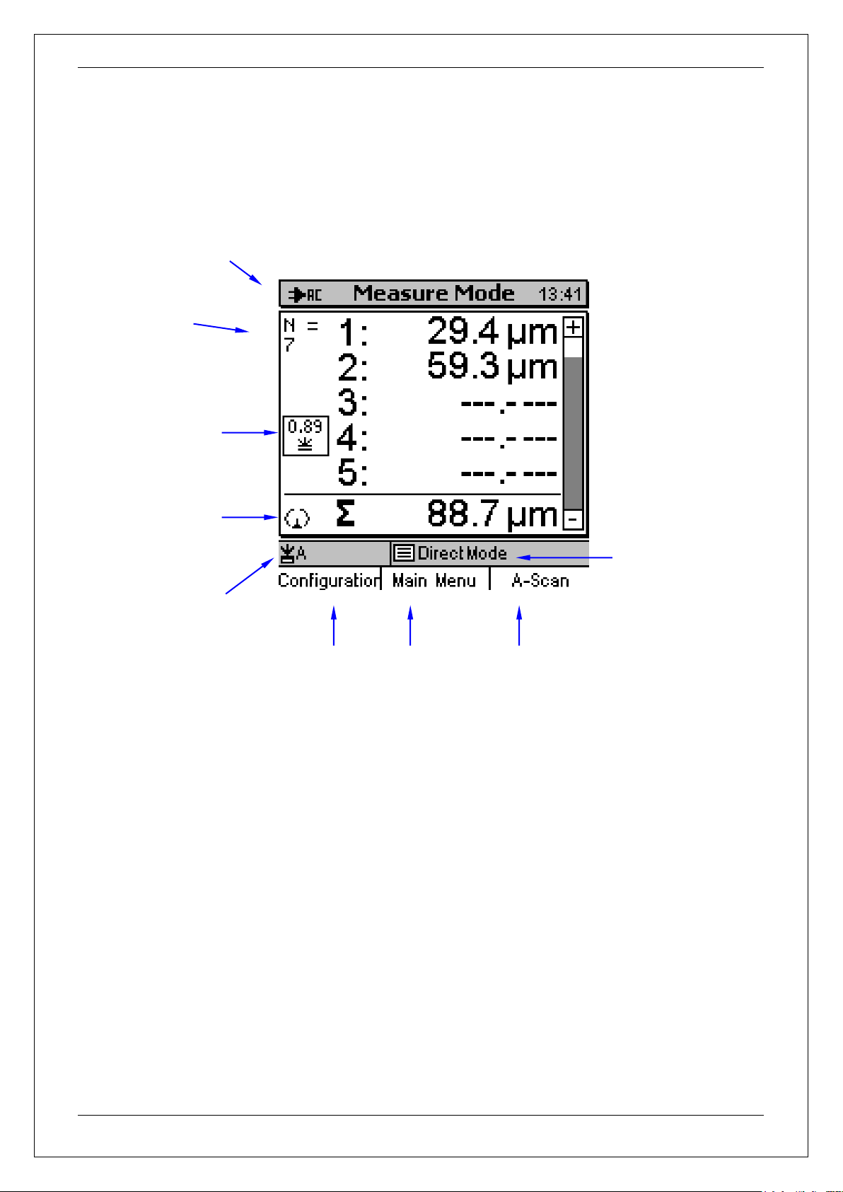
4.1.3 Measure mode – Large numerical screen

Mains or battery operation

with state of charge

Time

Layer thickness 1 Layer thickness 2

Active

parameter set

Antenna icon,

flashing if

sensor is

connected

Active batch

Number of

readings

Coupling index

Total thickness

Current property of function key

User Interface

If a good readability of readings has priority, it is recommended to call the numerical screen as shown above. This screen is only includes readings and some additional information such as coupling index and number of readings. This screen offers sufficient space to represent large numerical values to enable good readability from the distance.

To call this screen the “Graphics” parameter must be disabled. Go to the “Configuration” submenu

and press the “Configuration” function key (see section 15 5. 3 “Configuration”).

4.1.4 Measure Mode – A-screen Image with Echo Signal

Current property of function keys Layer thickness 1

Amplitude value at

cursor position

Crosshair cursor

Time value at cursor position

Here the function keys assume cursor move functions

Time

Amplitude zoomdetail [%]

Coupling index

Mains or battery operation

with state of charge

Time [ns] on the left edge of screen

Time [ns] (on the right

edge of screen)

Echo pulse

Echo line

Clipping limits

Percentage [%] for clipping limits

Zoom and position indicator

Layer thickness 2

User Interface

This screen represents the behaviour in time of the so-called echo signal that has been computed from the measuring signal. The time axis runs from left to right with the time values being displayed on the left or right side respectively.

The extracted echoes are represented as vertical lines within the echo pulses. Each echo is marked with an icon to indicate its state and origin.

On the left screen, the thickness of the individual layers is displayed as a numerical value. The A-scan image includes a crosshair cursor that can be used for moving along the signal curve.

This enables you to read the amplitude value at any point of the curve (numerical value on the upper right of screen).

The broken lines represent the clipping lines. For their signification and use please refer to section

8. The A-scan image also includes a zoom function to zoom in or out sections as requested (see also

section 7.4).

User Interface

Current properties of function keys

Mains or battery operation

with state of charge

Active

parameter set

Time

Active batch

If a reading is taking whilst the A-scan image is being active, the reading will be immediately shown on the A-scan image (see section 7.4.6). A previous change to the measure screen will not take place.

For a detailed description of the A-screen, its significance and how to use it, please refer to sections 7 and 8.

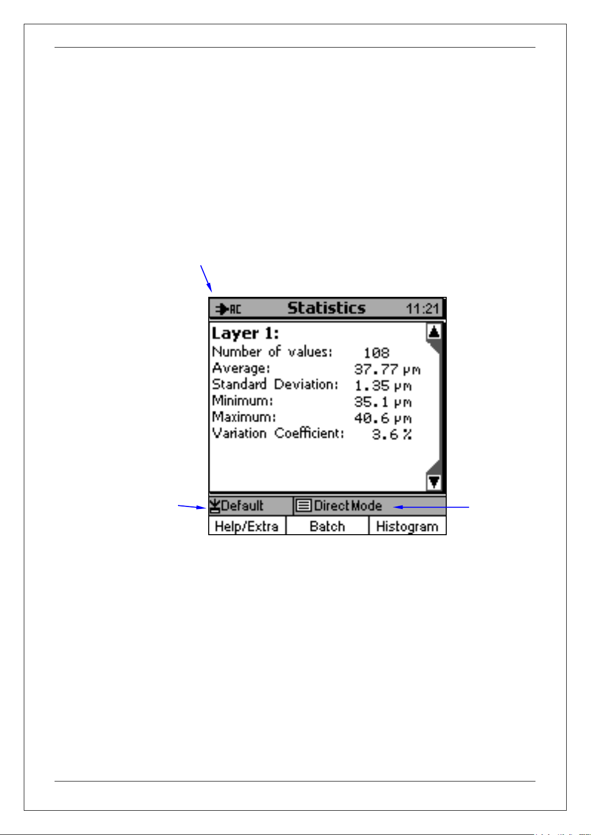
4.1.5 Statistics screen

All statistical values of a batch will be reported in tabular form. The figure above represents Layer 1. Statistics are available for each individual layer as well as for the total thickness. For more details on the statistical functions please refer to section 13.

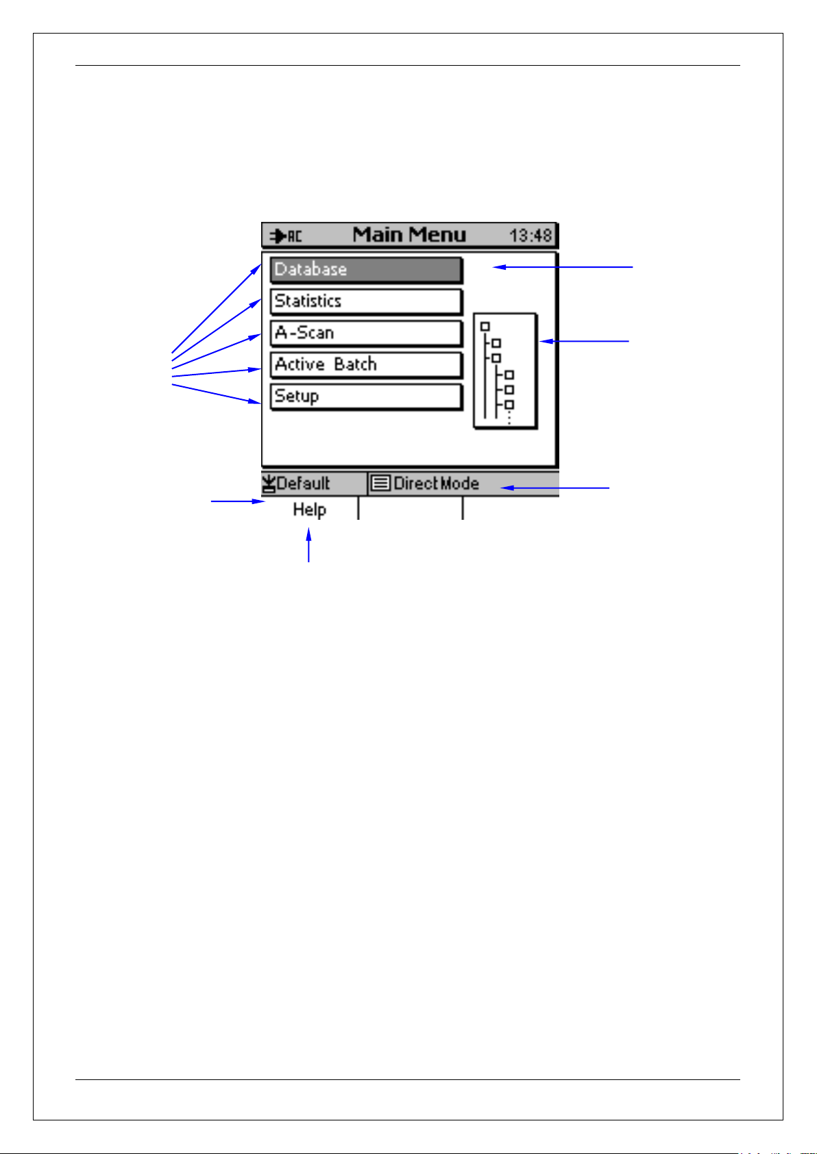
4.1.6 Main menu

Active

parameter set

Active batch

Submenus

Icon for your selected menu item

Selected menu item

Main menu help

User Interface

The figure above shows the main menu. It is the highest menu level (start level). From numerous

screens, this menu can be accessed via the function key “Main Menu”.

Press ”Main menu“ and use the arrow keys to scroll through the submenus. Press OK to confirm

your submenu selection. From any submenu you can return to the main menu by pressing the ESC-key repeatedly. If you

press ESC in the main menu, you will go back to the measure screen. The typical items of a menu are shown on the figure above. Press the Help-key on the left to call up the help menu relating to the currently active menu. A

context oriented help is available for many of the different screens. For more detailed information please refer to section 4.2.

User Interface

4.2 How to navigate in the main menu

The numerous QuintSonic 7 functions can be accessed via the hierarchically structured user menu. The main menu represents the highest menu level. From the main menu you can get access to various submenus and their respective submenus or to other screens such as statistics or parameter screens. In this section, a few examples are given to show you how to navigate through the menu.

Press function key “Main menu” to call the main menu. Note: Some of the screens do not feature a ”Main menu“ function key. In such case, please press ESC repeatedly until you access a screen

featuring such key.

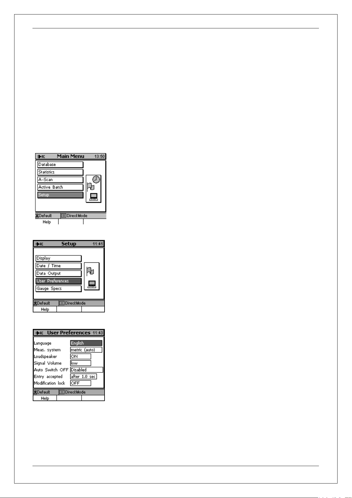
From the main menu, press arrow-up or -down key to select the requested item, for instance “Setup”. Press OK to confirm. The selected item will be called up.

The „Setup“ menu includes a submenu. Use arrow keys to select

“User Preferences” and confirm by OK to call up your selection.

The “User Preferences“ menu does not lead to submenus but it

includes a list of parameter options. The following section 4.3 provides more information on parameter options.

Press ESC-key to go back to the previous menu level. If you press ESC from the main menu, the measure screen will appear. By means of the above navigation instructions you can move through the complete menu and access any menu as requested.

User Interface

4.3 Parameter setting

Many of the screens do not represent submenus but list parameter setting options. Most of the parameters are user adjustable. Their setting may vary according to the type of parameter. In this section, a few examples are given to show you how to set the different types of parameters.

Your parameter selection will be highlighted in grey. Use the arrow-keys to scroll through the options. If you scroll down over the maximum, the cursor will skip aback to the beginning. This is for quicker setting action. The cursor does only mark your parameter option without making any changes to it. How to reach the editing mode for changing a parameter will be explained in the relevant sections relating to the different parameter types.

Some of the parameters cannot be changed such as “active batch” / “batch properties”. You will

quickly identify such parameters if no selection cursor is available.

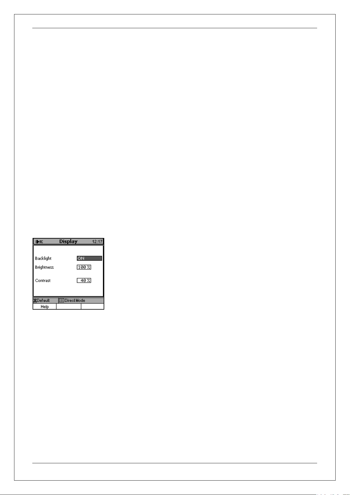
4.3.1 Setting a switch parameter (Example: Backlight)

Some parameters only offer two settings such as on/ off or

enabled/disabled. This kind of parameters are referred to as “switch

parameters”.

Example: “Backlight” from the submenu “Setup\Display”.

Select “Setup” followed by “Display” and choose “Backlight”.

Press OK and the parameter will change its state. If you press again, it will switch back, etc.

The state highlighted state is being active.

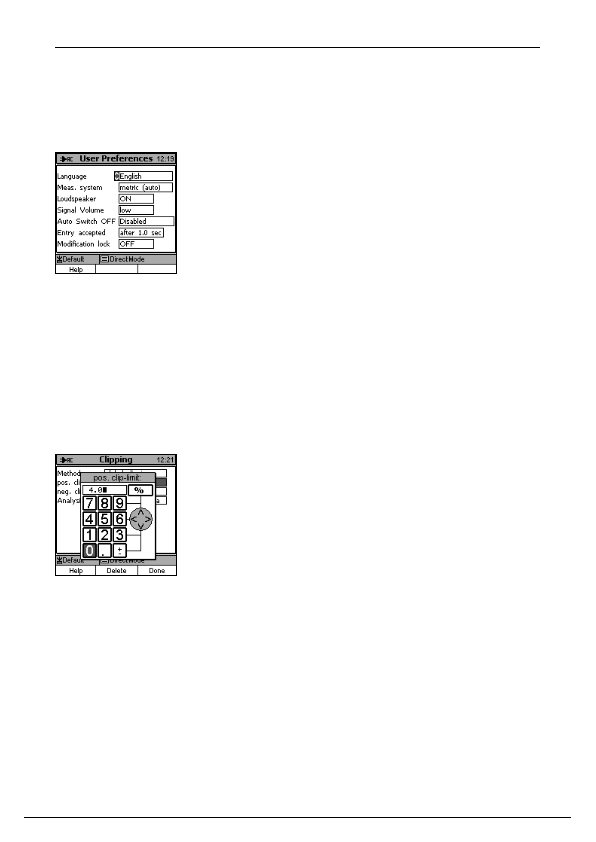
4.3.2 Setting selection parameters (Example: language)

Selection parameters offer more than two states.

Example: “Language” from the submenu “Setup\User Preferences”.

Select “Setup” followed by “User Preferences” and choose

“Language”. Press OK to confirm.

On the left of the options field an arrow up/down symbol will appear to indicate that you can now set this parameter.

Use the arrow keys from the navigation block to scroll through the options. Press arrow keys until you reach your requested option, e.g. “English” and press OK to confirm. Your setting has become active and the arrow symbol disappears. If you do not want to change the setting, press ESC instead of confirming by OK.

User Interface

4.3.3 Setting a numerical parameter (Example: pos. clip-limit)

Some parameters require a numerical setting. Once you select such parameter, a special entry screen will appear.

Example: “pos. clip limit” from the batch configuration menu. See

section 12.1.2.1 “Clipping”.

The ESC- and OK-keys assume navigation functions to the left/right. The arrow keys assume their standard navigation function up/down. The entry method is similar to writing a text message on a mobile

phone. Use ESC, OK or arrow key to move the cursor over the numerical entry field. Once you have reached the requested value, wait until the auto-save time delay has passed and the value will be accepted automatically. The auto-save time delay can be set via

Setup/User Preferences/ Entry accepted: after….sec. See section

15.6.5. If you wish to enter the same value again, just move the cursor to any

other value and go back immediately to the requested value. If you have mistyped, you can delete the unwanted value from the entry line by pressing the “Delete” function key. If necessary, press repeatedly.

User Interface

Shift key enabled

Once you have entered the requested value, press the “Done“ function key. A confirmation query will appear. Press OK to save this value as parameter setting. Press ESC if you do not wish to save changes. In such case, the previous setting will remain valid.

4.3.4 Alphanumercial parameter entries (Example: directory name)

When setting a parameter that requires an alphanumerical entry, a special entry window will appear.

Example: How to enter a directory name when creating a new subdirectory (see also section 11.2.2.1).

You may generate a name of 15 characters maximum. The ESC- and OK-keys assume navigation functions to the left/right. The arrow keys assume their standard navigation function up/down. The entry method is similar to writing a text message on a mobile

phone. Use ESC, OK or arrow key to move the cursor over the alphanumerical entry field. Once you reached the requested character, wait until the auto-save time delay has passed and the value will be accepted automatically. The auto-save time delay can be set via Setup/User Preferences/ Entry accepted: after….sec. See section 15.6.5.

If you wish to enter the same character again, just move the cursor to any other character and go back immediately to the requested character. If you have mistyped, you can delete the false character

from the entry line by pressing the “Delete” function key. If necessary,

press repeatedly.

For typing one single capital letter, first navigate to „Shift“. An arrow

will appear to indicate the Shift key is enabled. Once you have entered the capital letter, the arrow will disappear. This mode is the default factory setting.

For permanent input of capital letters, move to the CAPS-field. Enabling the CAPS-field sets an input mode in which all typed letters are in upper case (and vice versa). A bold-typed arrow will appear to indicate the CAPS-key is enabled.

User Interface

The ”Special Character“ field offers another window for special

characters (also for vowel mutations). Once you have entered a special characters, this window will close automatically.

Once you have completed your text, press “Done“ to confirm. You will

be asked whether to save changes or not. Press OK to confirm or ESC to abort. If you abort, the previous setting will remain valid.

Calibration

5 Calibration

5.1 Particularities of ultrasonic coating thickness measurement systems

In ultrasonic measurement, the primary measured variables are the differences in travel times of the various components of the transmit and receive signal. In ultrasonic coating thickness measurement, travel times range from a few nanoseconds to several hundreds of nanoseconds (a nanosecond (ns) is one billionth of a second). The precision at which such travel times can be measured directly influence the accuracy that can be achieved for measurement. The SIDSP®sensor of the QuintSonc 7 is a crystal oscillator based time measurement system with a typical accuracy of 50 ppm (0.005%). This value is so small that, in practical operation, it can be neglected against all other factors that might impair accuracy. Unlike the conventional measuring methods used for coating thickness measurement, the QuintSonic 7 measuring system does not need any calibration. However, there is one decisive factor of influence resulting from the measuring object itself that you must be calibrated for: the sound velocity in the material to be measured.

When converting the differences of travel times as determined in the measuring object into coating thickness, the sound velocities in the individual layers act as constants of proportionality. These variables are properties of the measuring object, not of the measuring system and depend on the material and temperature involved. Most times, these variables are not exactly known. As a consequence, their determination through indirect methods is required. Most times this is done through optical evaluation of a material cross-section. Once determined, the variables can be made available to the measuring system in the form of a sound velocity calibration. This explains why the sound velocity calibration is vital for the precision of an ultrasonic coating thickness gauge.

5.2 How to calibrate for the sound velocity

QuintSonic 7 offers several methods for a sound velocity calibration. The methods are described in the following section. For the practical operation, please refer to section 12.1.4.4.

a) Enter numerical values for the sound velocities

A prerequisite for this method is that the numerical values of the sound velocities are know for each individual layer. For calibration, simply enter these values manually into the sound velocity table of the current batch. This method is very simple. In practical operation, however, this method is not applicable, as in most cases, the sound velocity of the materials to be measured is not know.

Calibration

b) Using the table of literature values

The QuintSonic 7 menu offers two selection tables from which you can choose a sound velocity according to the material to be measured.

In the table of ”literature values“ you will find a list of commonly used plastic materials and

other materials such as steel, brass, wood, etc. Once you have defined a layer by selecting a material from the table, the calibration for this layer is completed. Repeat this procedure for all layers of the layer system. Please note that the values listed in the literature value table are average values only. Due to material variations, the actual sound velocity of the material to be measured may deviate significantly from the values indicated in the table.

c) Using the table of „User values“

In this table you can define your own material / sound velocity combinations and define the different layers of your layer system accordingly. Once you have defined the different layers and their matching sound velocities, the calibration is completed. If the sound velocities have been confirmed by reliable methods such as a material cross-section, the “User values” table represents an excellent method for a quick and easy calibration. However, it must be considered that variations of raw material or batch-related product variations may be present. For that reason it is recommended to verify regularly whether the sound velocities you have defined in the table are still applicable for the material batch to be measured. If not, it is recommended to make a cross section of the new material batch and use the calibration standard resulting from this material cross section accordingly.

d) Using the preset value for industrial coatings

The sound velocities for most industrial coatings are in the range of 2375 m/s ±15%. If this default value of 2375 m/s is used for measuring industrial coating systems, as a consequence, a maximum error of ±15% can be expected (the sound velocity will be included in the calculation of coating thickness as a constant of proportionality). This is not good enough for absolute measurements. For some applications, however, the main aspect is focussed on keeping an absolute coating thickness constant that has previously been determined by another measuring method (cross-section). In such case, the displayed absolute value has little significance only. For that reason, it is recommended to carry out measurement on a reference sample. The individual layers of this sample should represent the same thickness as the target thickness to be expected. The displayed readings that to not match the actual coating thickness, will be used as setpoint for the measurements to follow. All further measurements will only provide the variations from the setpoint. This is important for process control, for instance. In this connection, default sound velocities can be used to a limited extend only. However, this does not represent a calibration in the strict sense. For the configuration of a measuring series, QuintSonic offers to use the above value as a preset value.

Calibration

e) Calibration using a defined coating thickness (calibration standard)

For this method, a so called calibration standard must be available. The layer composition of such standard must be the same as that of the object to be measured.

The individual layers of the standard have been determined previously by another measuring method such as a cross-section, for instance.

Now enter the defined values of the individual layers into the table. Once completed, use QuintSonic 7 to take several measurements on the calibration standard. For each layer, the gauge will calculate an average from the set of readings you have taken.

Make sure to use the same measuring spot as during measurement with the other method. Of course, after a cross-section, this will be possible to a very limited extend only.

The system now processes the deviations from the thickness values that have been entered previously and the sound velocities are calculated accordingly. The sound velocities can later be used for further measurements. The calibration procedure is completed at this point.

As the calibration accuracy determines the accuracy of later measurement, the calibration procedure should be carried out under optimum conditions. It is highly recommended to take a reference signal before starting the calibration (see section 6.4.1).

Measure Mode

6 Measure Mode

6.1 Important remarks on ultrasonic measurement

Before using QuitSonic 7, it is recommended to read this information carefully. Make sure to understand and follow the instructions in order to avoid errors during measurement that might lead to erratic readings. Erratic readings can have serious consequences and lead to personal injury or damage to property.

Particularities with ultrasonic coating thickness measurement systems

After careful perusal of this manual you will be able to operate the QuintSonic 7 gauge correctly. Please note that apart from operating errors, there are a lot of other factors that might impair measurement.

Special attention should be paid to sections 6.2 to 6.5 and 7 to 9 providing essential information on the properties and particularities of measuring objects within the scope of ultrasonic measurement. In addition the above mentioned sections, this manual include instructions on the steps required to prepare measurement, on the use of the sensor, on how to avoid interference and on the correct interpretation of measuring results.

Skills required for operating the gauge

For using an ultrasonic measuring system, a basic training in the field of ultrasonic measuring techniques is recommended to make available sufficient knowledge on the following topics:

Theory of sound wave propagation Effects of the sound velocity in the measuring object Behaviour of the sound waves at the layer interfaces of different materials Propagation of the sound beam at the measuring point Influence of sound attenuation in the coating materials and influence of the surface structures

of samples

For training and support in the field of ultrasonic coating thickness measurement, please contact ElektroPhysik.

Preparing measurement (see also sections 6.3 and 6.4 For using an ultrasonic coating thickness gauge, it is necessary to take a certain number of

preparatory steps such as:

Setting the correct parameters to the measuring system Calibrate the measuring system (see section 5)

Setting the measuring range (number and position of measuring points)

Measure Mode

Setting the processing parameters (limits of readings, admissible standard deviation, etc.)

The person in charge of measurement shall be responsible to instruct any person involved in measurement on the necessary preparatory steps and to make sure they are carried out appropriately. Any experience with similar measuring objects might be a useful base for such preparatory works.

6.2 Limits to the measurement technique

As any measuring technique, also the ultrasonic coating thickness measurement is subject to certain limitations – mostly of physical nature. The following section will refer to such limitations, their origin and how to deal with it.

Formulating conclusions to non-inspected areas

The results obtained from measurement solely relate to areas of the sample that have been inspected. Conclusions to other areas of the measurement object are not admissible. They are only allowed if extensive experience on the process of manufacture is available and if appropriate methods for statistical evaluation can be applied.

Differences in acoustic impedance

The acoustic impedance values of layer interfaces must vary sufficiently in order to ensure the reflection coefficient at the layer interface is high enough for being evaluated. If this is not the case, the ultrasonic thickness measurement is pushed to its physical limits. If impedance values do not vary sufficiently, a clear separation of the layers is not possible any more. For more details please refer to sections 7 to 9.

Sound velocities

Ultrasonic coating thickness measurement is based on the measurement of travel times taking into account the sound velocities in the individual layers. For the calculation of the layer thickness, it is presumed on the assumption that the velocities in the individual layers are known and constant. For reliable measurement, all conditions must be fulfilled. As the sound velocity is used as a constant of proportionality to calculate the coating thickness, a sound velocity error of 5% will result in the an error of 5% accordingly. For that reason, it is vital to adjust the correct sound velocity.

If the sound velocities of the materials to be measured are not known (as this generally is the case with industrial coatings because of strong material variations that may occur), it is required to determine the sound velocities prior to measurement. This can be done by means of an optical evaluation of sample cross-sections. First the cross-sections of samples are measured by means of the QuintSonic 7 gauge. After this, the measuring system can be calibrated according to the results obtained by the cross-section. Through the calibration procedure, the correct sound velocities will be adjusted automatically.

If a material presents discontinuities (caused by the manufacturing process, for instance,) the sound velocity in this material may vary. The variations may occur continuously or in steps. In such

Measure Mode

case, an average sound velocity should be used. To determine the average sound velocity, a sample cross-section should be made for optical evaluation. If the sound velocity jumps at certain points, additional sound wave reflections will be produced at such points and lead to erratic readings if disregarded (see also section 7.3.3.5).

If dramatic changes of the sound velocity are to be expected (e.g. if two material batches vary due to different production parameters), it is recommended either to readjust the sound velocity within shorter time intervals or to adjust to the actual batch-related sound velocities. This is to avoid erratic readings.

Wall thickness measurement

Measuring objects with steel bases mostly exhibit a constant sound velocity in the base, even if the alloying elements vary. For wall thickness measurement of the steel base, it is important to know that the variations of sound velocity are so small that they can almost be neglected as far as their influence on the measuring precision is concerned.

In other materials, however, such as non-ferrous metals or plastics, the sound velocity is subject to higher levels of variation that may impair the measuring precision. For that reason it is required to determine the sound velocity by means of a suitable method such as mechanical thickness measurement of the uncoated sample. For thinner bases, it is recommended to make a material cross sections.

Also strong sound attenuation may impair measurement. It occurs in some kinds of plastic materials, for instance. In such materials, sound attenuation becomes stronger with increasing wall thickness. When reaching a certain material thickness (depending on the type of material), the sound attenuation is so strong that the amplitude of the reflected sound wave will not be strong enough for being processed. This may be the case with plastic materials of around 1 to 2 mm thickness. For such materials, the ultrasonic method is not suitable. If you have a new measuring tasks, it is recommended first to create an A-scan image (see section 17) to check whether the amplitude of the receive signal is strong enough to ensure reliable testing.

Variations of the sound velocities as function of material temperature

The sound velocity is also influenced by the temperature in the material layers. The temperature coefficients also depend on the type of material with some materials exhibiting a non-constant temperature profile.

The QuintSonic 7 sensor features an integrated temperature compensation for the sound velocities of layers. The temperature compensation is adjusted to an average temperature coefficient of typical industrial coating materials.

The temperature compensation will only work if sensor head and measuring object have the same temperature. Generally, ultrasonic coating thickness measurement systems are not able to record the current temperature distribution within a layer system that could be used for correction accordingly.

Measure Mode

For that reason, larger measuring error may occur if a cold sensor is placed on a warm measuring object or vice versa. Whenever possible, it is recommended, prior to measurement, to provide for a temperature adjustment of sensor and measuring object.

Good results can be achieved by storing sensor and measuring object in the same room for a period of about 15 or better 30 minutes prior to measurement so that sensor and measuring object can adapt to the ambient temperature accordingly.

In the ideal case, measurement should take place under the same temperature conditions under which the determination of sound velocity has been carried out. In such case, the different temperature coefficients in the individual layers will no longer have an effect on measurement.

6.3 Settings to make prior to measurement

Before taking readings, it is required to carry out some settings via Main Menu / Active Batch. QuintSoinc 7 store readings in batches. First create a batch and store in under a name in the

database. The name you have assigned to your batch is shown on the measuring screen. New readings will be added and stored to the currently active batch. If you switch the gauge off, the name of the last batch you have used will be memorized so that you can continue in this batch even after a switch off.

6.3.1 Using the Direct Mode

For quick, rough or trial measurements, QuintSonic offers a permanent batch named “Direct mode“. In this mode, no storage or processing of data or parameter settings are made. For quick access to this mode, select “Database” from the “Main Menu”. The “Direct Mode” is placed on top

of the highest directory level. In this mode, you can proceed immediately on the trial measurements. There is no need to make any entries such as name of batch or other. The parameter values of the last action in this mode are active. You can either continue in this setting or change parameters if required.

Use this batch for quick measurement action and if data processing or storage of parameters settings are not required.

For using the “Direct Mode” go to the database and select “Direct Mode” (see also section

11.2.3.5).

Measure Mode

6.3.2 How to create or select a batch

If you wish to store parameter settings or store and process readings, do not use the Direct Mode. For such purposes, you should use a standard measuring batch. Such batch can be created or selected as follows:

Create a new batch in the data base (see section 11.2.3.1). Select an existing batch from the data base (see section 11.2.3.5). Continue in the currently active batch.

Choose one of the options in order to assign the active batch for taking readings.

6.3.3 Selecting a measuring range

Prior to the preparatory steps for a new measuring task, it is required to choose a suitable measuring range. Please refer to section 12.1.1 for more details on how to select a measuring range.

QunitSonic 7 offers 5 time-measuring ranges (see section 3.2.2). Please refer to section 19 for the matching coating thickness ranges based on an assumed sound velocity of 2375 m/ s (average value for industrial coatings). As the sound velocity is a constant of proportionality, twice the coating thickness can be measured within the same measuring range if the sound velocity is double. Compared to plastic materials, the sound velocities in metal coatings are much higher (approx. 6000 m/s). As a result, in metal coatings, higher coating thickness ranges can be covered.

The total coating thickness of paint coating systems rarely exceeds a total of 300µm. For that reason, most times the measuring range # 1 (300 ns) applies. For wall thickness, however, larger measuring ranges are required.

For setting an appropriate measuring range, it is recommended, first to carry out a trial measurement. Make sure, all echoes of this trial measurement can be represented in one A-scan image (see section 7). If, for instance, echoes are missing on the right screen edge, the adjusted measuring range is too small. In such case, just try the next range.

If you are not sure about the appropriate measuring range, choose a larger one for a start. Once the echoes roughly located, you can switch to a smaller range but make sure no echoes will get

lost at the respective measuring range limits. Please do also refer to section 9.2 (Section 9 “Tips

and tricks”).

Measure Mode

Option 1: via the main menu

Press Main Menu-function key. Select “Active Batch” from the list. Press OK to confirm. The “Batch” menu is active.

6.4 How to prepare Measurement

6.4.1 Taking a reference signal

For processing a signal emitted by an ultrasonic sensor, an appropriate reference signal is required. QuintSonic 7 autonomously checks the validity of the existing reference signal. If the reference signal is invalid, you will be asked to take a new reference signal (see screenshot below). If the reference signal is valid, you can directly proceed on measurement. The reference signal is retained in the non-volatile memory to ensure it will be available even after the gauge has been switched off.

A reference signal may become invalid due to one or several of the following incidents:

You have switched the measuring range. The current temperature varies too much from the temperature during the acquisition of the

reference signal.

Generally, the acquisition of a reference signal is only required if such message appears. In order to ensure optimum precision of the system or if very difficult measuring tasks are involved (e.g. very thin coatings, low echo amplitudes), it is recommended to refresh the reference signal prior to

measurement (see section 9 “Tips and tricks”).

It is also recommended to take a reference signal prior to calibration (see section 5 “Calibration“).

For taking a reference signal please proceed as follows:

Measure Mode

Select “Configuration” from the list. Press OK to confirm.

The “Configuration” menu is active.

Select “Sensor reference measurement“.

Press OK to confirm.

To take a reference measurement, proceed according to the instructions.

Once the procedure completed, the Measure Mode screen will appear.

Option 2: via the Measure Mode screen

Press “Configuration“function key. The “Configuration” menu will be active.

Proceed according the steps as descried under option 1.

6.4.2 Selecting a couplant

In ultrasonic coating thickness measurement, couplants are needed to provide optimum transfer of ultrasonic wave energy between sensor and measuring object. Main target is to ensure both, a maximum input of energy as well as a maximum output of energy (of the receiving signal). For this purpose, the couplant must feature appropriate acoustic properties.

Measure Mode

Air is a totally unsuitable couplant and does not provide any results. Even if the sensor head is firmly pressed onto the object to be inspected, an air gap will remain. Hence, the use of a suitable couplant is vital for measurement.

QuintSonic 7 can be used with three different types of couplant:

clean water (preferably distilled water) glycerin (included in the supply schedule) ElektroPhysik coupling gel (supplied as an option)

With the above listed couplants, the viscosity (as a measure of the „thickness“ of a fluid) increases from water to coupling gel. Generally, you can assume the lower the viscosity, the thinner and more regular the coupling layer will be. The thinner and more regular the coupling layer has been applied, the better will be the coupling quality. As water tends to drip or run off from the measuring spot, especially from sloped surfaces, glycerin or coupling gel (if necessary for very difficult applications) will proof to be the better choice. Also for curved surfaces, coupling gel will provide the better results. The high-viscosity of such gel will – to some extent - better fill the gap between sensor and the curved object.

The suitability of the above listed couplants for this application has been carefully checked and approved by ElektroPhysik. If other couplants are used, user is responsible for measuring errors or damage to the sensor. Please note that any warranty claim will expire if the sensor is damaged by use of couplants other than those approved by ElektroPhysik.

6.4.3 Checking / carrying out calibration

Prior to measurement, it is recommended to check calibration. If necessary, proceed on recalibration (see also section 5). For rough or trial measurements in the Direct Mode (see section

6.3.1) or if no high accuracy is required, it is not necessary to calibrate and you can skip the

explanations below. If the gauge has been switched off and if you wish to continue the same setting of task in the same

batch, the calibration generally remains valid so that you can continue in this setting. However, make sure you are exactly dealing with the same measuring task. Any confusion with other, similar measuring tasks is to be excluded.

If you switch to another existing batch, the calibration stored for this batch will become valid and does generally apply for the measurements to follow if exactly the same measuring task is involved. If, however, the acquisition of readings in this batch dates back to a longer period of time or if any doubts regarding the validity of calibration for the measurements to follow arise, you should check the calibration or recalibrate, if necessary. For calibration, use a similar material sample. The thickness of the different layers of this sample must be known (calibration standard).

Measure Mode

When creating a new batch, you can take over the calibration from an existing batch. This is recommended only, if exactly the same measuring task is involved. Please see also section

11.2.3.1 “Creating a new batch”.

For a new measuring task, it is vital to calibrate for this task. If material cross-sections of the sample to be measured are available, it is recommended to use the optical evaluation of such cross-sections for the calibration procedure.

Taking readings without using a valid calibration only serves guiding purposes (to obtain an A-scan image, for instance). Reliable readings (numerical coating thickness values) will certainly not be provided.

6.5 Taking Readings

6.5.1 How to use the sensor

To ensure reliable readings and to ease the measuring procedure, the following recommendations should be observed:

Connect the sensor prior to switching the gauge on. Do not pull the sensor cable. For disconnecting the cable from the gauge or sensor, grasp the

corrugated sleeve of connector and pull to disconnect.

The measuring surface of the sensor is made of a special plastic material ensuring an optimum

ultrasonic energy transfer. Keep the sensor away from organic solvents, unsuitable couplants, hot or sharp-edged items.

The sensor has been designed for measuring smooth and flat surfaces. Rough surfaces may

damage the sensor or lead to erratic readings. Scratches on the sensor surface have an adverse effect on sensor resolution and reproducibility of readings.

After measurement and if you want to take the gauge out of service, use a moist and soft cloth

for cleaning the sensor surface. Dried up residue of couplant on the sensor is hard to remove and the sensor might be damaged when trying to clean from such residue.

Measure Mode

6.5.2 Measuring procedure

Prior to measurement, the preparatory steps according to section 6.4 must be carried out.

Make sure both, the surface of the measuring sample and sensor are clean and free from dirt

or couplant residues. Fresh paint must be dried out. Any contact with fresh paint, lacquer or varnish might cause irreversible damage to the sensor.

Choose a suitable couplant to apply to the measuring spot. The proper dosage and application

of couplant requires a little practice. When using water as couplant, a large drop will be sufficient as it will spread evenly once the sensor is put onto the sample. Coupling gel should be spread evenly over the measuring surface to ensure a uniform contact. If the gel emerges from under the sensor, you have used to much gel. On the other hand, an insufficient quantity of couplant will lead to interruptions during measurement as a reliable coupling cannot be ensured any more. During measurement, a coupling index will be displayed. This index will help you to learn to apply the proper dosage. Try to keep a constant coupling index. If during repetitive measurements a drop of the coupling index can be observed, the coupling contact has deteriorated and action to improve the coupling contact must be taken accordingly. The maximum coupling index depends on the nature of object to be measured.

For measurement, grip the grey, spring-mounted sensor sleeve to hold the sensor between

your thumb and forefingers (see fig. below).

Place the sensor vertically on the measuring object. Push the spring-mounted sleeve down to

the stop. Make sure the complete diameter of sleeve comes into full contact with the measuring object (only possible on flat objects). If by error, you have put the sensors in sloped position onto the measuring object, the sensor will automatically readjust once you have fully pushed the sleeve down. The corrugated sensor sleeve facilitates to use the correct contact pressure.

Now measurement and calculation of the coating thickness are carried out. This procedure

takes approx. 1 second.

Wait for the audible signal to confirm measurement has been completed. Then lift the sensor

from the measuring object.

The measuring results will be displayed and stored to the statistics memory. The total thickness

is shown as well as one or several individual layers (according to measuring object). See fig. below.

When taking repetitive measurements on the same spot, take care of the state of couplant. It

must not dry up. If necessary, remove the used couplant and apply a new quantity. Make sure the couplant is evenly distributed over the measuring surface.

Ideal sensor position.

Measure Mode

Example: Readings taken on a 3-layer sample

Signification and Use of A-scan Images

7 Signification and Use of A-scan Images

7.1 Introduction

Unlike conventional coating thickness measurement techniques (such as magneto-static, magnetic induction or eddy currents principles), the ultrasonic method represents a time domain measuring procedure. With this procedure, the measuring results to not depend on an instantaneous value but on the time curve of the primary measured variable. This time curve includes information on the individual layers of the measured layers system. Given this background, the ultrasonic method provides a kind of data evaluation and interpretation different from those provided by the conventional methods. The following section describes in detail the type of data evaluation and interpretation provided by QuintSonic 7.

The time curves are usually represented in X-Y diagrams with the X-axis indicating the time scale and the Y-axis indicating the amplitude scale of the measuring object. The measured variable as a function of time is shown as a closed curve running from the left edge (start time) to the right (end point). Each point on the X-axis is associated with a certain point, the amplitude value of which can be read from the X-axis. In ultrasonic measurement techniques, this type of time diagrams are commonly referred to as “A-scan image. “

Like with the classical coating thickness gauges, also with the QuintSonic 7, data acquisition and evaluation are made automatically. Once the sensor is put onto the measuring object, the measuring procedure will launch automatically and the results are shown on display. Thus, additional graphical representations do not seem to be necessary at a first glance. However, it should be considered that many factors may influence ultrasonic measurement, impair the evaluation of readings or lead to calculation errors. Sources of error may be insufficient coupling, discontinuities within in the layers (such as cavities, material inclusions, etc.) or noise interference due to coarseness of the coating material. Also multiple reflections should be taken into account. By making the correct gauge settings, such interference can be eliminated in order to ensure reliable and reproducible results.

A-scan images are the ideal tool to identify improper conditions or interferences. Once the error source detected, you can quickly take the necessary steps to remedy to the problems. For instance, by making the correct settings. QuintSonic 7 offers comprehensive but manageable parameter setting options.

This section is a guide on how to interpret A-scan images. It will describe the different types of Ascan images along with their significance. Further you will find hints on noise suppression and examples will be given for the effects of the latter. In section 9 you will additional tips and tricks for special situations. Section 10 will provide some application examples.

Basically, the use of A-scan images is recommended, especially if you switch from one measuring task to another. Also if unexpected measuring results have been obtained, the A-scan image can be of assistance. Experience has shown that if A-scan image and measuring results are

Signification and Use of A-scan Images

P A N

correlating, it can be assumed that measurement has been correct. That’s why the verification of readings by means of the A-scan image should become a routine in ultrasonic measurement.

7.2 Description of A-scan Image Types

QuintSonic 7 provides the following types of A-scan images:

reference signal raw measuring signal echo signal with echo lines

The different A-scan images result from the different stages of the measuring and evaluation process. Their information content and use is also different and will be described in the following section.

All A-scan images are scaled in time units (nanoseconds). As the sound velocities vary according to the individual layers, it is not possible and would make no sense to scale in thickness units.

7.2.1 Reference signal

Example of an A-scan image with reference signal

The above figure is a typical example of an A-scan image that should be generated and stored in the background if a reference signal has been taken (see section 6.4.1). It exactly reflects the representation of the reference signal received by the ultrasonic sensor head.

Signification and Use of A-scan Images

A proper reference signal always consists of a positive pulse (P). This pulse almost reaches the positive maximum (approx. 95%). It is followed by a smaller negative pulse (N), followed by a flat reverberation time (A). The complete signal curve should represent a smooth progression without sudden jumps or sharp bends (Note: Here, it is not referred to the small steps caused by the restricted graphics resolution).

7.2.2 Raw measuring signal

Example a raw measuring signal A-scan image

This is an example of an A-scan image generated and stored in the background if a measuring signal has been taken. This kind of A-scan image will be generated at any launch of a measuring procedure, irrespective of whether the coupling to the measuring object has been successful or not. It exactly reflects the representation of the measuring signal received by the ultrasonic sensor head. A-scan profiles are not uniform but strongly depend on the properties of the object to be measured as well as on the coupling performance. The above figure shows an example for a measuring signal. As with the reference signal, the signal profile should be smooth without jumps or sharp bends. There are no further requirements for a proper A-scan image.

The above A-scan image does not allow to deduce any statements with respect to the position of the layer interfaces. This is because the individual echoes overlap and thus would result in a totally misleading overall image. In this A-scan image, a maximum pulse does not inevitably represent the position of an echo. Echoes are often located in zones of low intensity or even in zero passages.

If measurement has been accidentally launched by pushing the sensor sleeve and the sensor was clean and has been held into the air, the A-scan image that results from this action will be identical with the reference A-scan image. Please note that the A-scan image of the measuring signal is of no significance for the user, it only serves for servicing purposes. It is only mentioned in this manual for the sake of completeness and to enhance the understanding of the overall context.

7.2.3 Echo signal with echo lines

Coupling echo lines (Y, Z)

Layer echo lines

Clippinglimits

Time characteristic of echo signal with echo pulses

Signification and Use of A-scan Images

Example of an echo signal A-scan image

The above A-scan image represents the complete evaluation procedure. The graphical part of the image includes three elements:

The time characteristic of the echo signal as calculated by the processing algorithm. It is

represented as a continuous curve running from the left to the right. The signal comprises a number of positive and/or negative pluses such as the coupling echo pulse and the echo pulses of the echoes detected at the layer interfaces. According to measuring object, also portions of interference may be included such as interference pulses or noise interference. Such interferences can be suppressed by suitable filtering or selections methods described in section 8. In the above example, interference is very low.

Various horizontal and vertical limiting lines as well as colour-shaded or hatched zones

representing the filtering or selection measures for noise suppression as set by the user. The example above shows two horizontal broken lines indicating the global clipping limits. See also section 8.3.3.1. Other filtering or selection measures have not been taken and therefore they are not shown in the above example.

Extracted echoes resulting from the echo signal setting. These echoes are represented as

Not all pulses that can be seen in the echo signal are actually fitted with an echo line. This is due to the clipping processes as selected and set by the user in order to cut out certain portions of the

vertical lines. They take their start at the zero line and are marked with icons. Each echo has been extracted from an echo signal pulse and is therefore located within this pulse. Most times, the exact position and height is identical with the maximum pulse (see also 8.4 Least squares optimisation).

Signification and Use of A-scan Images

echo signal that shall be excluded from echo extraction for the purpose of interference suppression (see section 8.3).

The first two echoes marked ”Y“ and “Z“ indicate the coupling echoes between sensor head and

couplant and couplant and measuring object, respectively. They will not be taken into account for the determination of the number of detected layers and are always represented as broken lines.

All further echoes can be divided into two different groups:

All echoes represented as continuous line are valid echoes. They are numbered consecutively

and will be taken into account for the determination of coating thickness values.

All echoes represented as broken lines will be filtered out during the post-processing procedure

for various reasons and are invalid. Such invalid values are marked with an icon and will not be considered for the determination of coating thickness values. The icon identifies the reason why a signal has been recognized as being invalid. For further details on the icons and their meanings please see section 7.4.7.

The A-scan image of the above example gives an overview on the following information:

What does the echo signal determined by the signal processing algorithm look like? Which are the positions of the echo signal where echoes have been extracted? Which of the echoes have been identified and marked as being invalid and what are the

reasons for that?

What is the overall result of the processing procedure? Did the current parameter settings

make sure that only such echoes remain that do actually represent the layer interfaces?

This information directly relates to the various filtering and selection methods as described under section 8. The echo signal A-scan image serves for checking the effects of the current parameter settings.

Once a measuring signal has been taken, QuintSonic offers the possibility to continuously check new parameter settings by means of this signal. After each new parameter setting, the measuring signal will be reprocessed accordingly. This is to optimise the parameter setting by means of a fixed signal before you proceed on further measurements for checking the stability of such parameter setting. This procedure serves to facilitate the parameter setting procedure.

Some coating thickness gauge combine the raw measuring signal and the extracted echo lines in one diagram on the A-scan result image. This makes little sense as the raw measuring signal does not provide any precise information on the position of the echo. In addition, opinions vary as to the optimal temporal relation between the two diagram sections (Given the large temporal extent of the individual reflection components within the measuring signal, no clear link between raw measuring signal and extracted echo lines can be stated.).

Most times, the position of the extracted echo signals as compared to the profile of curve seems to be totally random. For that reason, on the A-scan image, QuintSonic 7 does not use the raw

Signification and Use of A-scan Images

measuring signal but the echo signal as calculated by the signal processing algorithm. This makes sure a clear time reference is given and the effects of parameter setting can be clearly identified. See also section 8 and the figure above.

7.3 Application

7.3.1 Reference signal

The reference signal A-scan image does not provide any information on the measuring object as it has been taken in the air as a medium. Its profile rather gives information on the state of measuring head an measuring electronics. For that reason it is used for servicing and diagnostics tasks. For calling this A-scan image please proceed according to section 16.3.2.

A proper reference signal should look like the example as described under section 7.2.1. The following section is dedicated to some divergent scenarios and the conclusions that can be drawn as a consequence.

No reference signal is shown, only a horizontal line. This indicates either a disconnection

between sensor head and measuring electronics or a failure of an electronic component.

The positive pulse P will not reach the maximum set point (approx. 95%). Either it is clearly

smaller or it reaches the upper edge of image (at a zoom factor set to 1) to finally to jump down (overshoot). The response characteristic is beyond the control range of the electronics. This may occur if the sensor head is damaged or worn.

The overall signal form clearly diverges from the image as shown under 7.2.1. The sensor head

is damaged or worn.

If the above symptoms appear, no further readings should be taken. Please send the sensor for checking / repair to the factory.

7.3.2 Raw measuring signal

This A-scan image does not include any relevant information for the user. It is only used in connection with the reference A-scan image for diagnostics or servicing purposes. For more detailed information please refer to section 16.3.2. Please note that the interpretation of this image is difficult and needs the skills and experience of trained servicing personnel.

7.3.3 Echo signal with echo lines

This A-scan image represents the main tool for the user. It includes all relevant information on the correct system parameter settings and the effects thereof on the echo signal. The below sections are dedicated to the different aspects of this subject. In some paragraphs it will be referred to

Signification and Use of A-scan Images

Coupling echoes (Y, Z)

methods and steps of echo signal processing. More detailed explanations on that will be given later on in section 8 “Echo Signal Processing”.

7.3.3.1 Coupling echoes

Example: coupling echoes

The first two echoes (marked “Y” and “Z”) present coupling echoes. As a rule, there are only two

coupling echoes to occur: a positive one (“Y”) for the transfer from the sensor head to the couplant and a negative one (“Z”) for the transfer from the couplant to the measuring object. As the couplant

is (or should be) thin, the two echo pulses mostly occur in immediate succession. The amplitudes (signal heights) fluctuate and depend on the nature and distribution of couplant as well as on the properties of the top layer of coating system.

The two coupling echoes should always be clearly represented. If they disappear through noise or if they are totally missing, this indicates a strong signal attenuation through coupling (soiled surface of measuring object or unsuitable couplant). If through signal attenuation the limits of Global Clipping will be undercut (see section 8.3.3.1), the measuring system will provide no results and an error message (coupling failure) will appear. In such case, it is recommended to clean the surface of measuring object at the measuring spot carefully and/ or to apply a suitable couplant.

If, on the other hand, the coupling echo “Y“ is too large, almost reaching the level of the reference

signal, a bad coupling can be assumed. This may be due to an insufficient quantity of or dried out couplant, an air gap caused by a slope positioning of the sensor or an uneven measuring object. In such case, please try to improve coupling by cleaning sensor head and measuring spot. After this, use fresh couplant.

The coupling index displayed during measurement indicates the quality of coupling. The higher the index, the better the coupling performance. However, the coupling index must not be misinterpreted as a factor, i.e. a couplig index increasing by 10% does not mean that the coupling performance has improved by 10%. The achievable maximum coupling index depends on the measuring object. Though the coupling index gives a useful hint with regards to the quality of coupling, the A-scan image will provide more detailed information on the conditions.

Signification and Use of A-scan Images

Noise components

The distance between the two coupling echoes presents the thickness of couplant layer. Make sure not to apply an excessive amount of couplant. If the two coupling echoes follow each other without space between each other, one can assume that the couplant layer was thin enough to ensure efficient coupling. If the coupant layer is too thick (as it often occurs when using coupling gel) the ultrasonic wave will risk to propagate in multiple travel paths. This may be due to various propagation paths in the couplant causing the pulse to enlarge. As a consequence, reproducibility of readings will be bad. To avoid such problems, it is recommended to apply only a thin layer of couplant.

In rare cases, the problem may occur that the acoustic properties of the couplant and the top layer of the coating system do not differ sufficiently in order to be distinguished from each other. As a consequence, there will be no negative echo even if the coupling is good enough. In such case it is recommended to use another couplant.

7.3.3.2 Noise floor

Example: noise floor

As the generated ultrasonic sound wave travels through the complete measuring object, not only the acoustic properties at the layer interfaces needed for coating thickness measurement will be represented but also the conditions in the layers themselves. Basically, no industrial coating material is totally homogeneous. As a consequence, small reflections will occur at material discontinuities, micro blowholes or inclusions. They will be represented as irregular course of the zero line (noise floor). The strength of noise depends on the object to be measured. QuintSonic 7 offers several selection methods usually suppress such noise almost completely.

By means of a suitable amplitude parameter clipping choice (see section 8.3.3) adapted to the object to be measured QuintSonic 7 enables to suppress the noise floor completely. The clipping

Signification and Use of A-scan Images

Layer interface echoes

limits should be set in a way that the following requirements can be met: On the one hand, the clipping limits must efficiently include the of noise components, on the other hand, the desired signal components must clearly be higher than the clipping limits (see fig. above). The different clipping methods enable a good adaptation to both: noise components being asymmetrical to the zero line and to noise components of a strength varying over the time.

Sometimes adjacent layers are very similar with respect to their acoustic properties. Hence, the sound reflections at the layer interfaces is very small. In such case, a compromise must be found between noise floor suppression and non-suppression of the layer interface reflections. The parameter setting must ensure to maintain all layer interface reflections. Any remaining components of the noise floor can be suppressed later on by means of the post processor (see section 8.5).

7.3.3.3 Layer interface echoes

Example: Layer interface echoes

Once the clipping parameters have been set correctly, apart from the coupling echoes, only the layer interface echoes remain after the preprocessor procedure has been carried out. These echoes will be fed to the subsequent post-processing procedure to finally give the coating thickness values.

In some measuring objects exhibiting blowholes, inclusions or other material discontinuities in a layer, additional echoes may occur that do not represent a layer interface. Please refer to section

7.3.3.5 for further details on such echoes.

Echoes at layer interfaces are numbered from the left to the right. The reference number corresponds to the single coating thickness values as shown on the left of screen.

Signification and Use of A-scan Images

7.3.3.4 Superimposed echoes

Echoes travelling in the same direction Echoes travelling in alternating directions Example: Superimposed echoes

If a layer is not thick enough, i.e. if the travel time through this layer is too short, the input and output echoes of this layer will overlap. The effects of this situation depend on whether the two echoes take the same direction or not (positive or negative).

If both echoes take the same direction, they will more or less merge into one large echo so that a detection of this layer will not be possible any more. A portion of the missing layer thickness will be added to the layer located above this layer, another portion will be added to thickness of the layer below. This explains why a reliable measurement of the complete layer system is not feasible any more.

If input and output signal travel in different directions, they will be represented on the diagram as directly adjacent echoes with different algebraic signs (positive / negative). In such case, a detection is possible. However, a suitable least-square optimisation (section 8.4) must be applied to make sure any incorrect echo position will be corrected accordingly. This will work within the temporal resolution limits of the system (see data sheet).

When measuring extremely thin layers, the temporal resolution does not allow to separate the input and output echoes any more. The travel times through such thin layers being very short, they have no significant effect on the calculated travel times of the adjacent layers and the thickness of the adjacent layers can be determined with sufficient accuracy. Only the extremely thin layer will not be represented in the result. A special situation will be given if additional layer interfaces have been produced due to interruptions of the manufacturing process (see section 7.3.3.5).

Signification and Use of A-scan Images

Echo pulse is too small

7.3.3.5 Missing or unexpected echoes

When measuring a new task, it may happen that the number of detected echoes (i.e. the number of layers) does not correspond to the number of layers to be expected. In such case, please check whether the number of expected layers is correct, i.e. make sure you do not mix up with other measuring samples. Another possible cause of error might be that the manufacturing process has been changed. Absolute clarity regarding the actual number of layers can only be given through a material cross section.

Example: missing echoes If adjacent layers have very similar acoustic properties and if through the coating process no

additional transitional layer has been produced, it often happens that a smaller number of echoes is generated. As a result, the generated echo amplitude is very small and will be obscured through the noise. In such case, the relevant layers cannot be separated from each other by means of the ultrasonic method. They will be displayed as one single layer. Their thickness will result from the sum of single layers. In the overall result, one layer will be missing. On the other hand, a wrong clipping parameter choice may lead to suppression of an echo that under normal condition should be good enough for being analysed. Such signal will not be show on the A-scan image. A glimpse on the echo diagram will enlighten this situation.

eliminated through clipping eliminated through blocked domain example: unexpected echoes

Signification and Use of A-scan Images

However, it more frequently occurs that more echoes than expected are produce. This may be due to the material irregularities of layers (inhomogeneities, etc.) as mentioned previously. If the unwanted echoes created by such irregularities are smaller than the echoes at layer interfaces, they can be removed by means of the amplitude clipping function. Stronger unwanted echoes should be removed by means of the post-processor function (see section 8.5). This function allows for instance to define domains for the blocking of unwanted echoes.

It should be taken into consideration that also certain production techniques may lead to the creation of additional echoes. As an example, some kinds of paint coatings tend to generate additional layer interfaces if the coating procedure of a layer has been interrupted. Tests carried out on industrial paintings have shown that interruptions of a few minutes only can produce a layer interface as shown on the A-scan image. The reflection at such layer interface can reach the size

of the “true” reflection at the layer interface. Though on both sides of the layer interface the same

material is present, a reflection and thus an echo is produced. This is because the material of the layer interface layer has changed under the influence of air so that the acoustic properties have changed accordingly. As the layer interface is very thin (beyond the resolution limits given by the system), its thickness will not be identified. As a consequence, only one reflection instead of two will be produced.

If such kinds of unwanted echoes are produced, a material cross section will provide reliable information regarding the number and position of layers. The cross section result should be used to identify the “true” layer interfaces. Any unwanted echo can be filtered out by means of the postprocessor.

Unwanted echoes are marked with an icon to indicate the reason why they have been filtered out (see section 7.4.7).

Signification and Use of A-scan Images

7.4 How to use the A-scan screen

The A-scan image includes all necessary information on the quality of measurement, probable interferences as well as on the currently set filtering and selection methods. To enable convenient reading of the A-scan image, QuintSonic 7 provides several adjusting options in order to optimise the currently visible image sections.

Zoom-in and zoom-out in amplitude direction Zoom-in and zoom-out in direction of the time axis Shift of the time axis (Pan)

Several proxies are available to facilitate interpretation of the visible image section.

A cursor is available to move along the signal curve and read individual amplitude values accordingly. This is to facilitate the numerical parameter setting.

The following section will describe in detail how to use the above help tools. Some preprocessor (see section 8.3) as well as some post-processor (section 8.5) parameters

can be set directly by means of the A-scan image. This can be done numerically or graphically. These parameters include clipping limits (section 8.3.3), blocked domains (section 8.5.4) as well as

the expectancy domains (section 8.5.5). Please refer to section 12.2 “Graphical setting of a

parameter set” for more information on the use of these functions.

Signification and Use of A-scan Images

Zoom-in (Time)

Zoom-

ut (Time)

Zoom-out

(Amplitude)

Amplitude value at

cursor position

Crosshair cursor

Time value at cursor position

Function keys to move the graphics cursor

Amplitude zoomdetail [%]

Time [ns] on the left edge of screen

Time [ns] (on the right

edge of screen)

Zoom and position indicator

The above figures include all details that will be referred to in the description to follow. All further information will be based on the above A-scan image indicating the full time and amplitude domains (100%). The signal curve is very small and not clearly visible. The settings as described below will allow you to optimise the image section accordingly.

Signification and Use of A-scan Images

7.4.1 Zoom-in and zoom-out in amplitude direction

Press arrow-up key in order to zoom-in the A-scan image by a small factor in amplitude direction. The current size of image section is indicated in percent on the top left. Press arrow-up key repeatedly until you reach an image section of 33% of the total image allowing you to make visible all echo pulses in this example. The maximum zoom factor (8) will provide an image section of 13% of the total image (rounded value).

To zoom out the A-scan image in amplitude direction press arrow-down key. The A-scan image will be zoomed by a small factor in amplitude direction (zoom-out). Press arrow-down key repeatedly until you reach the maximum image section of 100%. Both functions, zoom-in and zoom-out will be carried out symmetrically to the zero line, i.e. the zero line will always remain in the centre of image. A displacement of the image in amplitude direction is not possible.

7.4.2 Zoom- in and zoom-out in time direction

Press OK-key in order to zoom-in the A-scan image by the factor 2 in direction of the time axis. The currently set time domain can be read from the time limits located on the left and right bottom edge of the image. In the example, the zoom-in factor of 2 enables an optimum positioning of the echo curve on the image section. Press OK repeatedly to zoom in to the requested factor (max.

8). Press ESC repeatedly for zooming-out (min. 1).

Zoom-in and zoom-out will always be carried out symmetrical to the position of the graphics cursor (section 7.4.3). Place the cursor in the centre of the required image section before carrying out the zoom function. If, however, this action will cause the absolute time domain limits (0 and end of time domain) to be exceeded, the system will correct automatically by displacing the image section. In the example, the graphics cursor has been adjusted to the time value of 0 before carrying out the zoom function. Hence, the left time limit will be fixed at zero after zooming. Only the right time limit has changed.

Signification and Use of A-scan Images

7.4.3 Graphics cursor and displacement in time direction

The A-scan provides a crosshair cursor acting over the whole range of image section. This cursor is used for reading the signal values and displacing the image section in direction of the time axis.

Use the function keys “left” and “right” to move the cursor in time direction. When moving the

cursor, it will follow the signal curve, i.e. the crossover between horizontal and vertical cursor line will always be located on the point of curve assigned to the signal.

By moving the cursor you can run along the complete signal curve and read the corresponding amplitude values at any point of the curve.

In the example shown on the left, the cursor has been placed exactly at the point of time of the first layer interface echo line. The associated time and amplitude values are indicated as numerical values upper to the image section

Move the cursor to the right edge of screen. When reaching a certain position, the image content will jump by a certain degree to the left, i.e. the image section has been displaced to the right. The same applies if you move the cursor to the left edge of screen.

By repeating this action, you can displace the image section over the total measuring range (Pan). However, the point of time 0 or the limits of measuring range cannot be exceeded. If the total measuring range (zoom factor 1) is visible, no displacement can be made.

Signification and Use of A-scan Images

Point of start: The A-scan image is displayed.

Press function key “Help/Extras” to call the menu as shown on example

on the left. Select the top item of menu to call the context-oriented help. The next 4

items below refer to the graphical processing of some portions of the parameter set. They will be described in section 12.2).

The three remaining items are described in this section. With “Echo position” you can call the echo position of the current reading. “Zoom

100%” and “Auto zoom” provide two different zoom options. Select one

of the items and press OK to confirm.

7.4.4 Zoom and position indicator

On the upper screen section below the title line, a bar can be seen. This is the zoom and position indictor. This bar offers orientation within the time domain when the zoom- and Pan-settings are active.

The total length of bar (light) represents the complete measuring range. The dark bar located in the light bar indicates the current image section. Within the bar, a light vertical line is located. This line indicates the cursor position within the image section.

Note: If the total measuring range is visible (zoom factor 1), the light bar will be fully covered by the dark

bar.

7.4.5 A-scan image menu

The A-scan image offers its own menu with some additional functions. How to call and operate this menu will be described below.

7.4.5.1 Calling the menu

7.4.5.2 Calling echo positions

The echo positions [ns] and amplitude values [%] of the current measurement are shown in a list.

The echoes marked “Y“ and “Z“ represent coupling echoes. The extracted layer interface echoes are numbered consecutively. The

numerical values facilitate the numerical entry of parameter values such as time and amplitude limits as the numerical values of echoes give you some orientation.

To quit this screen press OK and the A-scan image will appear.

With this function you can set the A-scan image section to full size (total measuring range, amplitude 100%) and the A-scan reappears.

The Auto zoom function automatically adjusts the image section of the current A-scan image in a way that all echoes can be seen at maximum size (optimal image section). After carrying out this function, the A-scan image reappears.

7.4.5.3 Zoom 100%

Signification and Use of A-scan Images

7.4.5.4 Auto-Zoom

Signification and Use of A-scan Images

The echo has been sorted out by “sensor head multi-echo suppression” (section

16.3.4)

The echo has been sorted out by multi-echo suppression (section 8.5.2).

The echo has been sorted out by manual echo selection (section 8.5.3).

The echo has been sorted out by a blocked domain (section 8.5.4)

Echo beyond the adjacent domains of expectation (section 8.5.5).

The echo has been sorted because of admissible number criterion (section 8.5.6).

7.4.6 Measure mode with A-scan image being shown

Readings can also be taken during the A-scan image is being active. The results of measurement will be directly displayed as numerical values as well as on the graph. This allows you to make visible variations of the signal curve during the measuring procedure. In addition, information is provided on the coupling state and stability of parameter setting. This will help you to asses the quality of measurement before you finally proceed on the regular measuring operation.

Note:

Readings that have been taken during the A-scan image was active will NOT be taken over into the measuring batch or statistics as such measurements are for trial purposes only in order to find the optimum settings. That the readings will not be stored can also be recognized by the fact that no thickness readings will be shown when changing to the measure mode screen (section 7.4.8).

7.4.7 Icons to identify invalid echoes

Of echoes have been sorted out by the post-processor (section 8.5), they will be marked with an icon on the A-scan image. These icons provide information on why an echo has been sorted out:

Signification and Use of A-scan Images

7.4.8 Quit the A-scan image

After you have reached the total image section you can quit the A-scan image by pressing ESC again. The query as shown on the left appears. Press ESC to quit the A-scan image or ESC to stay with the image.

Echo Signal Processing

8 Echo Signal Processing

8.1 Introduction

The QuintSonic 7 sensor integrates a signal processing algorithm consisting of several complex mathematical procedures. This algorithm uses the ultrasonic receive signal to calculate an echo signal. In this echo signal, all reflections are present in the form of echo signals of different size and directions (positive / negative) and of different time offset. This echo-to-echo time offset finally provides the necessary information for calculating the layer thickness.

Apart from the echoes produced by the reflections at the layer interfaces (and thus marking the interfaces between layers), the echo signal includes further portions produced from different sources (see sections below). For that reason, the echo signal calculated from the algorithm has to be processed in order to sort out echoes required for the calculation of layer thickness. For this purpose, the QuintSonic 7 sensor disposes of a number of filtering and selection methods. Please refer to the section to follow for a detailed description of their function, parameter setting and application.

In many cases a simple parameter setting or the basic settings will be good enough for reliable measurement (see below). For difficult settings of task, however, it will be necessary to find the correct parameter setting in order to deal with high levels of interference in the echo signal. In such cases, an appropriate assessment of the A-scan image of the echo signal will be vital for reliable measurement.

For a new setting of task you should generally start with a basic setting suitable for your application. The gauge provides a series of basic settings for typical applications in the form of predefined parameter sets (section 11 “Data Management”). Choose a suitable pre-defined parameter set before you proceed on trial measurements. Take a few readings and view the A-scan image. In many cases, you will find valid results at this early stage, i.e. the number and thickness of layers corresponds to your expectations and measurement is reproducible. In such case you can proceed on measurement using the selected basic settings.

In other circumstances, the A-scan will provide information why measurement is not reliable. Change settings accordingly and repeat the processing. With QuintSonic 7, it will not be necessary to take new readings. After a few trials you will find the appropriate parameter settings. You can store this parameter set under a new name and use it for further applications of the same kind. It is recommended to verify the correct function of the parameter set by carrying out further trial measurements before proceeding on the regular measurements.

The described procedure might seem to be rather complicated at first view. Experience has shown,

however, that most users quickly get familiar with the standard “tools kit” and can take full

advantage of the same. The variety of tools enables you to make the correct parameter choice adapted to the physical conditions of nearly any kind of application suitable for being measured

Echo Signal Processing

with the QuntSonic 7. Please do also refer to section 6.2 “Limits to the measurement technique”

and section 10 “Application Examples” with hints on the procedure for some typical applications.

To assist for new measuring tasks or for inexperienced users, ElektroPhysik offers a parameter setting service. Please send us your material sample. ElektroPhysik will make a cross section of the same. One half of the sample will be used to analyse the layers of the coating system. The other one will be used for taking readings by means of the QuintSonic 7. This way, an appropriate parameter set can be determined along with the matching sound velocities. The parameter set resulting from this service will be made available to the user.

8.2 Levels of Processing

The complete measuring and analysing cycle by QuintSonic 7 is done in a fully automatic sequence. The procedure includes the following steps:

Measurement procedure Signal processing algorithm sequence Preprocessor sequence (preprocessing) Optimisation sequence Postprocessor sequence (postprocessing) Calculation of layer thickness

The measuring procedure, signal processing-algorithm and the calculation of thickness sequence cannot be influenced by the user. For that reason no further details will be given on this subject.

The preprocessing, optimisation and postprocessing sequence can be adapted to the measuring task by adequate parameter setting. The type and effect of parameter setting will be explained below in detail.

8.3 Preprocessing

8.3.1 General remarks

As described in section 7, a typical echo signal exhibits some portions of noise produced by microscopically small inhomogeneities in the layers or in the base of the measuring object. The preprocessor is designed to eliminate such unwanted signals from the echo signal. Its main purpose, however, is to determine the positions and amplitudes of the individual echoes within the complete echo signal. This procedure is referred to as “echo extraction”. In this context, the two coupling echoes always located at the beginning of the echo signal occupy a special position.

Echo Signal Processing

To ensure an optimal echo extraction adapted to your setting of task, different processing methods and setting options are available. All these method have one thing in common: they clip out the various portions of unwanted echoes from the echo signal. This procedure is referred to as “clipping” and is subdivided into two different methods. With the so-called “time-clipping”, the processing will take place along the time axis (x-axis). The limits used in time-clipping represent time values. With the amplitude-clipping, the processing takes place by means of different amplitude values in amplitude direction (y-axis).

After the clipping has been performed, the preprocessor will extract the echoes accordingly. This will be done by searching for echo pulses on the remaining curve section. The maximum of a positive pulse determines the position of a positive echo whereas the minimum of a negative pulse determines the position of a negative echo. The detected echoes will be represented on the echo signal A-scan image as vertical lines at their respective time positions.

8.3.2 Time-clipping

For processing reasons, the echo signal delivered by the algorithm always covers a time domain being a little bit larger than indicated by the set measuring range. The time-clipping will clip off all portions beyond the measuring range. Currently, the time-clipping is defined by the size of measuring range and cannot be changed.

8.3.3 Amplitude-clipping

By means of the amplitude-clipping, portions of the echo signal curve containing unwanted echoes can be extracted from the echo extraction. QuintSonic 7 offers three different clipping methods adapted to different settings of task. According to the clipping method, one or two adjustable limits are used. It depends on the limits whether echoes will be extracted from a part of a signal curve or not. According to the clipping method, the limits will cover either the total time domain of signal or only a part of it. The individual clipping methods and their effects will be described below in detail. The settings will always be indicated as a percentage of the dynamic range of amplitude. The dynamic range of amplitude is shown at 100% once the amplitude zoom factor is adjusted to 1 (see also section 7.4.1). To give you a hint for orientation: The amplitude of reference signal is always 94%; the amplitude of the coupling echo and of the layer signal echo are clearly below this value for all applications.

The two coupling echoes are mandatory for evaluation. During the verification procedure, the system will check for each measurement whether the coupling echoes are present and whether they are correct. If the check will provide a negative result, measurement will be null and void and

the error message “coupling echo failure” will appear. For that reason, when setting the clipping

parameters, make sure not to accidentally suppress the coupling echoes.

Echo Signal Processing

8.3.3.1 Global clipping

In the global clipping, two adjustable limits are available: an upper and a lower limit. These values are shown on the echo signal A-scan image as horizontal lines. The domain between these limits is referred to as blocked domain. Over the total time zone of the echo signal, all signal portions located in the blocked domain will be clipped off and thus will not be used for echo extraction.

The preset value for the upper limit is +3% and -3% for the lower limit. For most applications, the noise floor and small unwanted echoes will be reliably suppressed in this preset mode already.

Higher levels of noise floor or unwanted echoes require an adaptation of limits. The limits must be set in a way to make sure all wanted echoes will be reliably extracted in subsequent measurements even if slight amplitude variations are present. This way, a maximum noise suppression is given. For measuring multi-layer systems, the setting is determined by the weakest echo.

This method represents the standard clipping method and is the first method to be used for new settings of task. It is easy to apply, includes a parameter preset and is sufficiently good for a wide range of applications.

In the standard mode of global clipping, the criterion for the extraction of an echo is that the echo signal travels beyond the blocked domain exceeding its extremes (maximum for positive echoes, minimum for negative echoes) to finally travel back to the blocked domain. This requirement is met in most applications (see fig. above).

If echoes of the same algebraic signs (i.e. two successive positive or negative echoes) are located very close to each other it may occur that the signal curve between both echoes will not travel back to the blocked domain but remain beyond the same (for an example, see section 10.4). To enable

the extraction of the two echoes despite of this situation, the additional function „Evaluation of local

extremes“ can be used. This function activates a further parameter, the so-called “minimum step height”. Any signal displacement in echo direction exceeding the step height setting will be

extracted as an echo. To ensure reliable echo extraction, the value should always be set slightly below the actual step heights on the A-scan image. Make sure the setting is not too low, otherwise you may risk slight variations of the echo signal will also be interpreted as echoes. A value around

0.5% presents a good compromise. Basically, the evaluation of local extremes should only be

activated if no correct echo extractions can be achieved in the standard mode.

Echo Signal Processing

The parameter settings of the global clipping can be made numerically (see section 12.1.2.1) or graphically via the A-scan image (see section 12.2.2.2.1).

8.3.3.2 Domain clipping

This method allows you to divide the total time zone of the echo signal into different domains. After this, you can assign individual limits to each of the domains. This function is of advantage if the layer echoes exhibit very different heights requiring to make too big a compromise if using the global clipping.

The domain limits (time values) can be set graphically or numerical by means of a table. In the ideal case, each time domain exactly includes one single echo for being extracted. As the A-scan image indicates whether the respective echo is a positive or a negative one, it will be sufficient to set one limit value per domain.

The position of the echo to be expected and the position of the blocked domain depend on the direction of evaluation you have set. For positive limits, the peak of echo must be located upper to the limit and the blocked domain is below this limit and vice versa as far as negative limits are concerned.

Under normal condition, positive echoes are located above the zero line and negative ones below. The so-called base line of echo signal, i.e. the behaviour of echo signal between the echoes is either running on the zero line itself or in direct proximity to it. The direction of evaluation as resulting from the sign of limit (positive or negative) exactly presumes such behaviour. In some special applications, however, it may occur that the base line of echo signal strongly differs from the zero line so that positive echoes are below the zero, for instance. To remedy to such situation you can use the “inverse” function for individual time domains. This function will turn evaluation into the inverse direction enabling to extract also such kind of echoes .

The domain clipping parameters can be set numerically (see section 12.1.2.1) or graphically via the A-scan image (see section 12.2.2.2.2).

Echo Signal Processing

8.3.3.3 Variable clipping

Like the domain clipping, the variable clipping also divides the total time domain of the echo signal into adjacent domains. Each domain defines its own amplitude limit controlling the clipping function for this domain. The effect of amplitude clipping is the same as that of the domain clipping (see

sections 8.3.3.2). The “inverse” function is also available and is the same as with the domain

clipping. In opposite to the domain clipping, the time limits of domains, however, are not fixed but depend on the position of echoes detected. For that reason, the variable clipping does not feature adjustable time limits.

The first domain always starts at position 2 of the coupling echo. As soon as the first echo has been found by means of the matching amplitude limit, the system switches to the second domain and processing will continue with the amplitude limit of the second section. The second domain ranges until the position of the next echo being detected, the system switches to the third domain and so on.

Point of start and length of the individual domains hence are triggered by the positions of the detected echoes. With this method, exactly one echo is available at every end of domain once the clipping procedure has been completed. Advantage of this method: For each layer echo to be expected an optimally matching amplitude limit can be adjusted according to its height and direction without the need to take into account the size of adjacent echoes. In addition, the automatic time triggering ensures each echo will always be extracted together with its matching amplitude limit, even if a displacement of the echoes in time direction due to variations in layer thickness takes place. Any displacements to adjacent domains are not possible.

The variable clipping proved to be the most flexible among the three clipping methods. It is particularly well-suited if the amplitudes of echo layers are known (for instance from a preliminary A-scan image). For practical use, being independent from variations in layer thickness is of great advantage.

The variable clipping parameters can be set numerically (see section 12.1.2.1) or graphically via the A-scan image (see section 12.2.2.2.3).

The clipping methods are easy to apply as long as the layer echoes are larger than unwanted echoes (if any), i.e. the switching of the system to the next domain cannot be triggered accidentally through an unwanted echo (given the correct setting of the amplitude limits). In failure of this, any unwanted echoes have to be extracted first together with the wanted echoes to be later

Echo Signal Processing

suppressed by the postprocessor. This will only work reliably as long as the number of unwanted echoes does not change.

8.4 Least-Squares Optimisation

Due to the physical properties of the sensor head, the echo pulses that can be seen on the A-scan image exhibit a predefined pulse width, the so-called frequency band with. This band width cannot be undercut. When measuring very thin layers, their echo pulses converge on the A-scan image so as to border. If layers are even smaller, they may overlap causing the peaks of pulse to shift

slightly. That’s why also the extracted echoes exhibit a slight displacement. This situation

especially occurs if two echo pulses are available showing into the same direction (both echoes positive or negative).

In order to adjust for the deviations caused, the least-squares optimisation function can be used. This processing level does not change the position and size of echoes until the deviations from the correct position are minimised. This condition will be checked by means of the so-called method of least-squares.

The result of this adjustment procedure (optimisation) becomes obvious on the A-scan image. One can see that the echo lines are no more located exactly under the pulse maxima. Instead their position is slightly off-centred. Also the size of echo does not exactly correspond to the pulse heights any more. This does not present an error but it illustrates the effect of optimisation. The correct result is represented by the echo lines.

The use of this optimisation function is recommended particularly for thin layers as the individual thin layers imply short travel times. For industrial paints, the optimisation procedure should be considered for layers of 20µm and less. Adjacent layer echoes showing into different directions are less concerned than echoes showing into the same direction. In case of doubt, an optimisation trial should be made in order to verify the size of corrections and reproducibility of readings. If clear corrections occur and if measurements are reproducible, the optimisation function should be enabled for further measurements.

For more details on the optimisation please see also section 9 “Tips and Tricks”.

Echo Signal Processing

8.5 Postprocessing

8.5.1 General remarks

While the preprocessor is designed to extract the echoes from the echo signal curve by means of the set clipping parameters and to optimise their position and size (least squares optimisation), the postprocessor focuses on the selection of echoes. It aims to select from the extracted echoes only those to be used for layer thickness calculation. In other words, unwanted echoes produced by interference or noise will be identified and suppressed accordingly. For this purpose, a comparison with the results from a cross section is of great help as the echoes at layer interfaces can thus be quickly identified. Only the remaining echoes will be considered as being unwanted echoes and can be suppressed accordingly by using appropriate methods.

QuintSonic 7 offers a number of postprocessing options that partially complement each other or can be used alternatively. The postprocessor runs a set of possible selection mechanisms in a fixed sequence. If certain processing methods are not activated, they will be jumped. Each processing level identifies the echoes that have been suppressed and thus eliminated in this level accordingly. This makes sure that at the end of the postprocessing procedure it will be clearly shown by which selection criterion a certain echo has been suppressed and eliminated. On the Ascan image, the peak of suppressed or invalid echoes is marked by an icon (see also section

7.4.7). So you can quickly identify why a certain echo has become invalid. This will help you to find

out whether a selection has been incorrect and remedy accordingly. The following sections describe the selections methods available. They are listed according to their

running sequence.

8.5.2 Multiple-echo suppression

Some types of material (such as metals for instance) may produce strong echoes on both sides of the layer interfaces. This is due to strong variations of the acoustic properties at the layer interfaces and due to the weak attenuation of ultrasound in the material itself. Sound waves travelling between two layer interfaces produce multiple reflections. As the sound, however, will never be reflected completely, a part of the energy from each of the reflections will be sent back to the sensor head. As a result, multiple echoes will disturb the evaluation and thus lead to erratic

Echo Signal Processing

calculation of layer thickness. As multiple reflections exhibit special properties, they can be quickly identified and suppressed accordingly.

In the first instance, multiple reflections are characterised by a constant time interval between two adjacent echoes (The same distance is always covered at the same sound velocity). Another distinctive characteristic is the amplitude decreasing from echo to echo due to the sound attenuation in the material. The algebraic sign (positive or negative) of all multiple echoes generated in one layer can be either always the same or change alternately between positive and negative. This depends on the conditions being available at the layer interfaces.

If the conditions are given for the presence of multiple reflections (in metal bases, for instance), the

processing level “multiple echo suppression“ of the postprocessor can be used. Once activated, the “multiple echo suppression” will search for echo sequences in the echo curve that meet the

above described criteria. All matching echoes will be suppressed accordingly except the first echo of each sequence. The first echoes represents the “original echo”.

With certain layer/base combinations, adjacent layers (also several in a row) may happen to exhibit identical travel times and continuously decreasing amplitudes. All echoes from such layer interfaces are valid ones and do not represent multiple echoes. However, as they meet the criteria for suppression, they will be suppressed by the multiple echo suppression function. For that reason, the multiple echo suppression should be disabled for such applications.

8.5.3 Manual echo selection

This function allows you to select up to 8 echoes (coupling echoes included) from a sequence and define them as being valid. You can mark your selection in a table (see fig. above). All nonselected echoes will be suppressed accordingly.

This selection methods always suits if the number and sequence of layer echoes and unwanted echoes is known and constant and if no sporadic interferences occur that might temporarily change this sequence.

Echo Signal Processing

8.5.4 Blocked domains

This selection methods allows to define time domains by setting amplitude limits. A echoes being present with these limits will be suppressed accordingly. The time zero point is located on the time position of the 2nd coupling echo (“z” in the fig. above) ensuring the thickness of coupling layer will not be taken into consideration for processing.

The significance of the amplitude limits is the same as with the preprocessor domain clipping: a positive limit will suppress any echo the peak of which being below this limit. A negative limit will suppress any echo being above this limit. If you set limits higher than any positive echo in this domain or lower than any negative echo in this domain, all echoes will be suppressed in this domain. If you set to zero, there will be no blocking function at all. The purpose of such setting is to produce gaps between two blocked domains.

A maximum of 8 adjacent blocked domains can be defined. Each of the domains can be enabled or disabled individually. Each domain starts from the second coupling echo (starting point) and is characterised by an amplitude limit. A domain ranges from the starting point up to the starting point of the next active domain. Disabled domains will be jumped. If there is no other active domain to follow a starting point, the domain will range to the end of measuring range. On the A-scan image, blocked domains are characterised by dark, transparent areas to ensure the signal curve can still be seen.

Blocked domains are used to exclude complete continuous domains from evaluation. This is of good assistance when measuring inhomogeneous materials with many unwanted echo zones. The definition of blocked domains is also an appropriate and effective method for suppression of noise occurring beyond the base interface up to the end of the measuring range.

The parameters for defining blocked domains can be made numerically (section 12.1.4.2) or graphically via the A-scan image (section 12.2.3).

Echo Signal Processing

8.5.5 Expectancy domains

Expectancy domains are the opposite of blocked domains. All echoes located within the limits of expectancy domains will be taken into account for evaluation. Any echo beyond these limits will be suppressed. Particularity: expectancy domains are not related to fixed time values but to the

individual positions of echoes. They are to be considered as coating thickness ranges. That’s why

this method also very well adapts to layers systems with the thickness of the individual layers varying strongly. This situation will be described in detail in the following paragraph:

For using the expectancy domain method, the nature of the layer system must be known very well so that projections can be made as far as the thickness of the individual layers is concerned. Such information can be obtained from the results of a cross section, for instance. For each expectancy domain, the user must specify an upper and a lower limit to define the tolerance range within the limits of which the respective layer thickness values should be situated. For evaluation, these limits are always related to the position of the preceding valid echo. Thus it can be ensured that only the current layer will be considered, irrespective of the thickness of the preceding layers and their respective echoes positions.

Any echo located between the expectancy domains will be classified as being unwanted and suppressed accordingly. Only echoes located in the expectancy domains will remain. If several echoes are detected in an expectancy domain, the largest one will be marked as being valid, all others will be invalid. Any echoes located behind the last expectancy domain are considered as not being part of any of the expectancy domains and are also invalid.

Each time at least one echo has been detected in an expectancy domain, the system switches to

the next subsequent expectancy domain. That’s why a minimum of one valid echo will be assigned

to each of the expectancy domains. The width of tolerance range depends on the variance in layer thickness to be expected. The smaller the set tolerance range, the more effective the suppression of unwanted echoes.

The upper and lower limits (layer thickness values) result from the nominal value and its respective tolerance. An expectancy domain is completely defined by its upper and lower limits (layer thickness values). These limits result form a nominal value and the respective tolerances. An expectancy domain can be either enabled or disabled. Disabled domains will be jumped and

Echo Signal Processing

ignored during evaluation. On the A-scan image, an expectancy domain is shown as a blank rectangle (see fig. above). Its association to the respective layer is determined by its position in direction of the y-axis and corresponds to the column of layer thickness on the left edge of screen.

For layer samples of a know structure the use of expectancy domains is highly effective. Major

advantage of this function: processing adapts to the variance in layer thickness by “following” the

layer interface echoes. However, please note that not only the nominal thickness values must be known but also the tolerances limits. At least, the latter must be estimated as good as possible. If a layer thickness is beyond the set tolerance range, as a consequence, no echo will be assigned to the expectancy domain concerned. As the system will consider this situation to be an error, processing is stopped at this point. In such case, you have to correct the nominal value or tolerance limits concerned and repeat processing accordingly. It will also be a problem if several echoes can be found in one expectancy domain as you cannot be sure that the largest echo actually represents the right one. In the ideal case, the expectancy domains should be set in a way to make sure exactly the echo to be detected will actually be found in the respective domain. Any adjacent unwanted echoes should be located beyond this domain.

Expectancy domains should not be mixed up with the upper and lower limits from the statistics function. Expectancy domains serve for suppression of unwanted echoes. They are not meant to provide a base for the statistical evaluation of product quality (pass/fail recognition). For that reason, when setting expectancy domains, the focus should be put on reliable suppression of unwanted echoes as found on the A-scan image. Any settings for statistical evaluation can be made via the statistics module (see section 12).

The parameters for defining expectancy domains can be made numerically (section 12.1.4.3) or graphically via the A-scan image (section 12.2.4).

8.5.6 Number criteria

8.5.6.1 Number of layers

In this menu you can set the number of layers to be evaluated. Generally, this number is known to the user.

The number you have set in this menu will be used by the criteria “First echoes”, “Last echoes” and “Largest echoes” as described later in the paragraph.

Echo Signal Processing

8.5.6.2 First echoes

The number of layers you set in this menu (2 in the above example) defines the maximum number of echoes (starting from left to the right) to be used for processing. If the number of echoes detected is less than the number of layers you have set, the system will identify less layers accordingly. “First echoes” is the default setting.

8.5.6.3 Last echoes

From the right to the left, i.e. starting from the last echo, the system will evaluate at maximum as many echoes as you have set layers (2 layers in the above example). If the number of echoes detected is less than the number of layers you have set, the system will identify less layers accordingly. This setting is of advantage for the evaluations of wall thickness irrespective of the number of layers detected. If you adjust the number of layers to be detected to 1, the system will only evaluate the wall thickness. If you set this number to > 1, the system will always consider the last thickness value to be the wall thickness.

Echo Signal Processing

8.5.6.4 Largest echoes

Starting from the largest echo, the system will evaluate the echoes subsequently according to size. At maximum, as many echoes as the number of layers you have set will be evaluated (2 in the example above). If the number of echoes detected is less than the number of layers you have set, the system will identify less layers accordingly. This setting is of advantage if the size of all layer interface echoes is clearly different from the size of unwanted echoes. This way, you can skip any further complicated selection method.

8.5.6.5 Final remarks

Some of the above selection methods can only be used separately, i.e. you cannot use two or more methods at the same time. This applies, for instance, for the settings described under 8.5.6.2 to 8.5.6.4. Overlapping or contradictory effects will therefore not occur.

On the other hand, some of the selection methods that can be usefully combined so as to complement their effects. As an example, combining “First echoes” (section 8.5.6.2) with number of layers =2 (section 8.5.6.1) will determine both, the position and the number of echoes to be detected.

Make sure not to combine selection methods in a contradictory kind of way that might lead to unexpected results or results difficult to interpret. For example, it will be contradictory if you manually select 5 echoes (section 8.5.3) because you expect 5 layer thickness values and at the same time, adjust the number of layers to 2 (section 8.5.6.1). As a consequence of such setting, only 2 thickness values would appear instead of 2.

Tips and tricks

9 Tips and tricks

9.1 Cross-section

If you have got a new setting of task, it is highly recommended to make a material cross-section of your sample before you proceed on measurement. Such material cross-section (which is to be made only once) will be a valuable base for the assessment of your sample and for the interpretation of the A-scan image. In addition, it will be of good assistance for making the correct parameter settings. A cross section provides the number and position of layer interfaces, hence you can perfectly distinguish layer interfaces from interferences on the A-scan image. This is vital for the choice and setting of filtering and selection methods.

There are not many industrial plants having the facilities for making such material cross-section with the required precision and for optical measurement by means of a calibrated measuring microscope. For that reason, ElektroPhysik offers a cross-section service with later optical evaluation of the sample. It is highly recommended to use this service: If the sound velocities in the materials concerned are not known, such cross-section evaluation will be required anyway for obtaining reliable and precise measuring results.

9.2 Measuring range

It is recommended always to choose the smallest possible measuring range for your setting of task. Make sure always to work at the maximum possible resolution in order to obtain highest precision and reproducibility of readings. A measuring range higher than necessary will result in deviations of readings due to quantisation and rounding errors.

The optimal, smallest possible measuring range has been found once you can see all relevant echoes on the A-scan image (at a zoom factor = 1). It will not be necessary to choose a larger measuring range only to make echoes visible being of no interest.

9.3 How to proceed for a new setting of task

For a start, it is recommended to use the minimum of means for a new measuring task. A good base will be the following parameter setting:

Clipping method: global clipping ±3% Optimisation : OFF Number of layers: unknown Echo selection method: First echoes Blocked domains: disabled

Tips and tricks

Expectancy domains: disabled

These are the settings of the „Default parameter set“ used for the creation of a new measuring

series (provided you did not take over the settings of the previously used measuring series). Basically, the default parameter yields useful results for a large number of applications.

Carry out a few trial measurements and view the results on the A-scan image. If the number of readings to be expected has been recognized reproducibly and if the layer thickness values meet your expectations or are identical with the cross-section results, it will not be necessary to change the parameters any more. However, if you observe that due to interferences, an excessive number of echoes or unwanted echoes have been extracted, or if echoes are missing, it is required to reset the parameters accordingly. First you have to find out the nature of problem and think about the

best parameter choice in order to settle the problem. “Wildly experimenting” will not lead to

satisfying results. The first step is to change a time parameter and view the results of the resetting before you

proceed on the next parameter change. As long as you are not familiar enough with the system, it is not recommended to change several parameters at the same time. The effects of such parameter reset would be difficult to assess and probably lead to unnecessary, time-consuming procedures but to no avail. However, once you are familiar with the system, a short glance on the A-scan image will be sufficient to assess how make the correct parameter choice. Two or three further steps will be enough to lead you to your objective while it will even be possible to set several parameters at a time.

9.4 Amplitude clipping with optimisation enabled

If optimisation (section 8.4) has been enabled, it is recommended to set the amplitude clipping to a minimum just high enough to ensure a reliable filtering of noise and very small interference echoes. Single, larger interference echoes should not be suppressed by clipping in this case. For filtering such echoes, the postprocessor should rather be used. This procedure makes it easier for the optimisation procedure to make corrections more exactly. As a result, the measuring precision will improve.

9.5 High level of unwanted echoes in the layers

For measuring samples with a high level of unwanted varying echoes (as it often occurs in inhomogeneous materials) it is recommended to disable the optimisation function (see 8.4) as the reproducibility of readings will improve if this function is disabled.

Tips and tricks

9.6 Inhomogeneous bases

For bases exhibiting strong material inhomogeneities such as GRP or CFRP, a blocked domain can be defined in order to filter out very strong unwanted echoes located beyond the base interface. Optimisation (8.4) should be disabled. Make sure the amplitude clipping level is set high enough in order to reliably remove noise being present within the limits of the useful range. In addition, it is recommended to limit the number of layers (8.5.6.1) in order to suppress any further echo beyond the specified number of layers.

9.7 Multiple reflections

Metal bases exhibit a strong variance of acoustic properties. Further, the attenuation of ultrasound in metals is very weak. For that reasons, very strong echoes are produced at both base interfaces of such samples. The sound waves travel back and forth between the base interfaces creating multiple reflections. As these specific properties are very characteristic for such multiple reflections, they can easily be identified and suppressed accordingly.

The multiple-echo suppression (8.5.2) can be used effectively to suppress such kind of echoes on condition that multiple reflections do not occur simultaneously in several layers (the base included). If they do, such echoes may overlap causing a displacement of the individual echo extremes. As a consequence, the conditions for identifying multiple echoes (constant distance) are not given any more and suppression will partially fail. In such cases other selection methods (such as the limitation of the number of layer) must be applied.

9.8 Measuring object of unidentified nature

If no precise knowledge on the nature and composition of a measuring object is available, it will be difficult to interpret the echo pulses that can be seen on the A-scan image and to distinguish interface echoes from interference echoes (if any). If adjacent layers have very similar acoustic properties, the echoes produced at their interfaces will be very weak. In such case, they cannot be identified via their amplitude size any more. It is quite possible that stronger interferences occur in

the vicinity (e.g. with “filled” materials) and will be misinterpreted as echoes sounding back from the

layer interfaces. For that reason, measurement will be erratic. Basically, the assessment and categorisation of echoes is rather unreliable unless you have a

minimum of information regarding the structure of a layer system. Any information (e.g. obtained from experience you have made with similar objects) regarding low interference levels, will improve the chance to obtain a correct evaluation as in such case, all strong and visible echoes can be

considered as being “real” echoes. However, no certainty will be given. Due to a very small

reflection factor you may risk to oversee echoes you might not expect at the instant of time concerned.

Tips and tricks

Unknown sound velocities represent another issue. Though the measuring results will provide the correct number of layers (on condition any other problems have not been encountered), you cannot be sure about the correctness of layer thickness unless you know the sound velocities in the materials concerned.

For that reason, it is always recommended to make a material cross-section. Based on the results of such cross section, you can interpret readings correctly and set parameters accordingly. This is the only way to obtain reliable and sound readings.

9.9 Interaction of preprocessor, optimisation and postprocessor parameters

This section is dedicated to experienced users wishing to obtain maximum system performance by using optimal parameter sets. A good understanding of the system functions is assumed.

The processing sequence – preprocessor, optimisation, postprocessor is of great significance for the determination of the optimal parameter set. The input data for the optimisation stage represent the output data of the preprocessor stage. In turn, the output data of the optimisation stage represent the input data for the postprocessor stage.

Using input data such as position and amplitudes of the extracted echoes, the optimisation process creates a synthetic receive signal. After this, the process tries in small steps to change the positions and amplitudes of the extracted echoes in a way that the respective, newly calculated synthetic receive signal deviate as little as possible from the true receive signal. This process is verified by using the least squares method.

The optimisation will succeed more effectively to the extent that the input signal of the optimisation stage is complete. If bigger portions of the input signal are missing (e. g. through a preceding clipping with amplitudes limits adjusted very high), the optimisation processor might try to close this

“gap” by displacing and enlarging extracted echoes located in the proximity. This will unnecessarily

deteriorate the accuracy of the neighbouring echoes. If the optimisation function is enabled, it is recommended not to suppress strong interference echoes by means of the preprocessor. They should rather be left in the signal for further use of such signal portions through the optimisation function. The interference echo portions can be suppressed later on by the postprocessor.

The postprocessor, with its various stages, represents the last processing level before calculation of layer thickness. The output signal of the postprocessor has no effect on the previous stage (preprocesor and optimisation). The processing steps of the postprocessor will only have an effect on the final result. For that reason, it is of no significance to the optimisation, how the postprocessor has been set.

On the other hand, the sequence of postprocessing stages is important. Please see section 8.5. An echo can be marked as being invalid only once. Once an echo has been identified as being invalid in a certain stage, it will be marked by an icon of this stage accordingly. As a consequence, it will not be considered any more in any further subsequent processing stage. If you find an echo marked other than expected, it is recommended to check at which stage it has actually been

filtered out. This situation occurs more frequently than expected, especially if several postprocessing selection criteria have been activated at the same time.

Tips and tricks

10 Application examples

10.1 Three-layer paint on plastic

Measuring range: 1 (300 ns).

Application examples

For measuring this setting of task you can use the preset parameter set (for values see section

9.2) without making any changes to it. The global clipping with ±3% limits will reliably remove any

noise floor (that is very low in the above example). All three layer interface echoes you expect will be extracted correctly. It will not be necessary to use the postprocessor function.

The thickness of the third layer is very thin and slightly ranges below the resolution limits of the system. Given their respective echoes 2 and 3 showing different algebraic signs, echo extraction will be no problem.

10.2 One-layer paint on wood

Measuring range: 1 (300 ns). Also for this measuring task you can work with the preset parameter set (for values see section

9.3) without any changes being necessary. The expected layer interface echo will be extracted

correctly. It will not be necessary to use the postprocessor function. However, there is one particularity to be seen on the A-scan image:

Application examples

Two very broad amplitudes are prominent: the amplitude of the second coupling echo (z) and that of the interface echo (1). This is due to the unevenness of the wood surface (as compared to the surface of a plastics base, for instance). The 3 mm diameter ultrasound beam hits the different peaks and valleys of the wooden surface. The portions of reflection are received by the measuring head at different instants of time to accumulate to the typical large pulse shape.

In addition, a very thick coupling layer can be observed, the traveling time in the coupling layer being almost 40 ns. This is also caused by the unevenness of the wooden surface. During the

painting procedure, such differences in height will not be completely compensated that’s why the

unevenness of the wooden base will be transferred to the paint surface. The measuring head only contacts the peaks of surface. The valleys are filled with couplant. If you add the pulse shape enlargement of the coupling echo (Z), a couplant thickness larger than the actual one will result as an average. You can also see from the A-scan image that the coupling index is not particularly high. This indicates the coupling performance is not optimal. However, you have to accept, as the situation cannot be changed.

Finally, a clear deviation of the base line from the zero line can be observed behind the interface echo (1). This is due to the increased noise floor caused by the strong granularity of the wood. In the above example, the clipping limit as set is high enough for noise floor suppression. If, however, the noise floor should increase during further measurements, setting the upper clipping limit to 4% can remedy. Another solution would be to define a blocked domain behind echo (1) or to set the number of echoes to be evaluated to 1.

10.3 Two-layer paint on steel

X-Zoom = 1 X-Zoom = 2 Measuring range: 1 (300 ns). Also in this example, the basic setting (for values see section 9.2) has been used. All expected

echoes have been extracted (1,2). Due to the small differences in the acoustic properties of layer materials, however, the first interface echo is relatively small (-3.6%). To increase the processing accuracy, it is recommended to reduce the negative clipping limit to –2%, for instance.

The large negative echo (2) is typical for a transition from plastic to metal. Metals always exhibiting a clearly higher acoustic impedance than plastics, the echo at the transitional layer will always be a large negative one. For that reason, such interface layers can be easily identified.

Application examples

Behind echo (2) a series of unwanted echoes can be observed. These echoes are multiple reflections from the second layer combined with artefacts from the metal itself. As behind echo (2) no further echoes are to be expected, the easiest way will be (as can be seen in the above figure) to define a blocked domain. If, however, the layer thickness i.e. the position of echo (2) vary significantly, it will be more reliable to reduce the number of echoes to be processed to 2 instead of defining a blocked domain. Otherwise, processing uncertainties might arise either because echo (2) will be suppressed or because the first unwanted echo located behind it will not be suppressed.

10.4 Thin one-layer paint on body sheet

X-Zoom = 4 X-Zoom = 1 Measuring range: 1 (300 ns). In the above example, a thin layer with a thickness close to the resolution limits of the system in

concerned. As a particularity, both echoes are negative ones, layer echo (1) as well the second coupling echo (Z). As a result, both layer echoes will partially superimpose causing the signal between the echoes not going back to zero. It will not even reach the blocked domain as defined by the global clipping. For that reason, processing by means of the basic setting will not be possible as the echo (Z) cannot be extracted.

However, a special setting of the global clipping function will enable echo extraction by activating the evaluation of local extremes (see 8.3.3.1 and 12.1.2.1). The so-called step height between coupling echo (Z) and the minimum located directly behind it will be examined. If the step height exceeds a preset value, the echo (Z) will be extracted. In the above example, the step height has been set to 0.5%. Considering the very clear signal curve, it may even be set to a lower value. You can see from the above figure that the echo (Z) has been extracted though the standard clipping criteria have not been fulfilled.

Furthermore, the back wall echo from the painted sheet has been extracted. It can be easily be suppressed by setting a blocked domain far away from the domain to be processed.

Application examples

10.5 Wall thickness measurement

Measuring range: 2 (750 ns). The same measuring object has been used as in section 10.3. Here, however, not the paint is to

be measured but the wall thickness of the metal base through the paint (coating). For a start, the basic setting has been used. On the right edge of the A-scan image the so-called

back wall echo can be seen with an amplitude of 13.5%. For that reason, the unwanted echoes in the middle of the A-scan image can easily be suppressed by setting the upper clipping limits to

8.5% so that only the relevant echoes will be extracted accordingly.

In order to display the wall thickness only, the postprocessor has been set to process the last echoes (from the rear to the front) only. The number of layers has been set to 1. As a consequence, the extracted echoes from the paint layers will be marked to be invalid (see fig.) and thus not taken into account for the calculation of layer thickness.

The sound velocity of “layer “ # 1 that remains after the postprocessing, must to set to the sound

velocity of steel. Using these settings will then provide the measuring results as shown above.

10.6 Multi-layer plastics foil

Measuring range: 2 (750 ns) In the above example, a coextruded foil of different materials is concerned. The thickness of the

individual layers varies significantly. To make sure all echoes will be extracted, the global clipping limits have been set to ±1%.

Application examples

Behind the second coupling echo, artefacts have been produced during the coupling procedure (probably multiple reflections in the couplant layer). For that reason, it was switched to domain clipping. The first clipping domain has been defined in a way to suppress the afore mentioned artefacts (see fig. on the right). The second clipping domain is operated in the global clipping mode with the amplitude limit set to 0 and ranging until the end of measuring range.

Five layer interface echoes have been extracted, hence five layer thickness values have been provided as a result.

Data Management

11 Data Management

11.1 Introduction

11.1.1 Batches

QuintSonic 7 stores readings and statistics to batches. To each batch a certain parameter set is associated. Such parameter set includes the setting parameters and the calibration stored for this batch. If you open an existing batch, the parameter set associated to this batch will become active.

To create batches and parameter sets, select Main menu / Database. The data management is a PC like file system. As usual, user definable subdirectories enable efficient data management. Subdirectories, batches and parameter sets can be named as you wish.

A predefined batch is stored under the name “Direct Mode”. This batch is fixed. Neither can it be deleted nor renamed (see 6.3.1). Use this batch for quick and rough readings and if there is no need for data storage or data evaluation.

11.1.2 Memory capacity / using the data memory

The memory of QuintSonic 7 disposes of a data memory for at total of 300 batches and parameter sets (e. g 200 batches and 100 parameter sets) to store a maximum of 250,000 readings.

Subdirectories with up to 5 levels are available to store and manage batches and parameter sets conveniently. The memory can be divided into a user-definable number of batches. For instance, you can use the complete memory for one batch only. Data storage is made automatically according to your requirements, i.e. it is not necessary to predefine the size of a batch.

11.1.3 Parameter sets

To each batch a parameter set is associated. Such parameter set includes all relevant settings for the respective measuring task:

Measuring range Settings for echo signal processing Sound velocities

Once you call a configured batch, the parameter set associated to it will automatically become active.

The Database facilitates data management of directories, batches and their associated parameter sets.

Directories with up to 5 levels are available to store a maximum of 300 batches along with the associated calibration methods and parameters settings. Via the directory you can choose configured batches, use them for further measurements or open batches for output of statistical information.

Press function key “Main menu” to call the main menu, followed by

data base. Press OK to confirm. All actions described hereunder will start from this point.

Use arrow keys up/down to move the cursor from its current position (greyed out) to the place on the tree where you wish to create a new directory. A new directory can be created at any place where the greyed out cursor disappears and the flash symbol appears instead (left screen). This is an intermediate position. A directory can be divided in to subdirectories.

Once you have found the requested position, press the function key “Actions”. Choose “New Directory” and press OK to confirm.

11.2 Data base

11.2.1 General remarks / How to call the data base

Data Management

11.2.2 Directories

11.2.2.1 How to create a directory

Data Management

The alphanumerical input screen appears. Enter a name for the new directory (see section 4.3.4 “Alphanumerical entries”).

Press OK to confirm your entry or ESC to abort.

Once you have confirmed your entry, the directory has been created and will be shown on the directory tree.

Use arrow up/down keys to select the directory or the directory entry (batch, parameter set) you wish to delete.

Your selection will be greyed out. Press function key “Actions” and select “Delete”. Press OK to confirm.

11.2.2.2 How to delete a directory or a directory entry

Data Management

A confirmation prompt will appear. Press OK to deleted the selected entry or ESC to abort.

Once you have confirmed deletion, the selected entry will be deleted and removed from the directory tree.

Note: You can only delete empty directories. Any subdirectories and/ or

batches and parameter sets must be deleted previously. This is a safety measure in order to prevent accidental deletion of data.

The “Direct mode “ batch cannot be deleted. A parameter set associated to one or several batches cannot be

deleted.

Caution!

Data will be deleted irretrievably and cannot be restored any more. For that reason, the delete function should be used with caution!

Use arrow up/down keys to select the directory or directory entry you wish to move. Your selection will be greyed out.

Press function key “Actions”. Select “Move” from the list and press OK to confirm.

Follow the pop-up window. The move procedure will be executed. Note: The target position must be an intermediate position, i.e. it must be

located between two entries or a the end of the tree. Such intermediate position will be marked by an arrow on the left edge of screen.

It may occur that during the move procedure a message will appear

“Memory optimisation in progress! Please wait…”. This is for internal

reasons only and not of any importance to the user.

The directory entry has been moved to the requested position.

11.2.2.3 How to move a directory or a directory entry

Data Management

Use arrow up/down keys to select the directory or directory entry (batch, parameter set) you wish to rename. Your selection will be greyed out.

Press function key “Actions”. Select “Rename” from the list and press OK to confirm.

The current name appears in the alphanumerical entry field. You can

change it now (see section 4.3.4 “Alphanumerical entries”. )The user

name will persist.

The name has been changed and the new directory name appears on the directory tree.

11.2.2.4 How to rename a directory or a directory entry

Data Management

Call the main menu. Select the submenu “Database”. Press OK to confirm. The submenu appears. Use arrow up/down keys to select the intermediate position where you

wish to insert a new batch. On the left edge of screen, a small arrow appears at the intermediate

position. You can create a batch at any intermediate position of the directory tree.

In the example on the left, this is the upper tree level.

Press function key “Actions”. Select the menu item “New batch” from the list.

Press OK to confirm.

A alphanumerical entry field appears. Enter a batch name (see section

4.3.4 “Alphanumerical entries”).

A confirmation prompt will ask you whether to save the new name or not. Press OK to confirm or ESC to abort the creation of a new batch.

11.2.3 Batches

11.2.3.1 How to create a new batch

Data Management

Again, the alphanumerical entry field appears. Now you can enter a user name (see section 4.3.4 “Alphanumerical entries”).

This entry is optional. Note: It is not possible to assign a name to the “Direct Mode “ batch.

A confirmation prompt will ask you whether to save the new user name. Press OK to confirm or ESC to abort.

To complete the procedure, a confirmation prompt will ask you whether to accept the settings from the currently active batch. Press OK to confirm or ESC to copy other presettings or make new settings

The copy function facilitates the creation of a series of new batches or to copy settings from the Direct mode.

The batch has been created and will appear on the directory tree. For parameter settings see section 12.

Press function key “Main menu” and select “Database”. Press OK to confirm. The currently active batch and its matching parameter set are shown on

the status line. Use arrow up/down keys to choose the requested batch and press OK

to confirm your selection.

Your selection has become active now. The batch properties of are shown on a list.

If you do not wish to make any changes to the batch parameter settings, you can directly proceed on measurement.

Place the senor on the measuring object. The gauge switches automatically to measuring mode and the currently

reading is shown. You may also press the OK key to switch to the measuring mode.

11.2.3.2 Delete a batch

Section 11.2.2.2 “How to delete a directory or a directory entry”.

11.2.3.3 Move a batch

See section 11.2.2.3: “How to move a directory or a directory entry“.

11.2.3.4 Rename a batch

See section 11.2.2.4: “How to rename a directory or a directory entry“.

11.2.3.5 Choose a batch for measurement

Data Management

Option 1: via the main menu

Press function key main menu and select “Active Batch” from the list. Press OK to confirm.

The submenu “Active Batch” will appear.

Choose “Configuration” and press OK to confrm.

The “Configuration” submenu will appear.

Choose “Parameter set” and press OK to confirm.

Choose a parameter set from the list and press OK to confirm.

11.2.3.6 How to assign another parameter set to an active batch

Data Management

ElektroPhysik QuintSonic 7 Technical Manual And Operating Instructions

Specifications and Main Features

Frequently Asked Questions

User Manual