

Page 1
MCE User’s Guide
Version 1.3
May 2004
Page 2
MCE User’s Guide
Copyright and Warranty
© 2000-2004 Kimmo Uutela. All rights reserved.
The author makes no warranty of any kind with regard to this material or the software.
This document contains proprietary information, which is protected by copyright. No part of this
document may be copied or changed without the prior consent of the author. The information
contained in this document is subject to change without notice.
This program was developed at the Brain Research Unit of the Low Temperature Laboratory in
Helsinki University of Technology.
The commercial distribution of the product for MEG analysis is exclusively licensed to Elekta
Neuromag Oy.
Included with the software are public domain software components:
• mysql_mex by Kimmo Uutela
• lpsolve_mex by Kimmo Uutela, Michel Berkelaar, and Jeroen Dirks
• Perl 5 by Larry Wall
• DBI by Tim Bunce
• DBD:mysql by Perl Jochen Wiedmann
• Berkeley MPEG Tools by The Regents of the University of California
See the source code of these programs provided with the software for copyright details those
components.
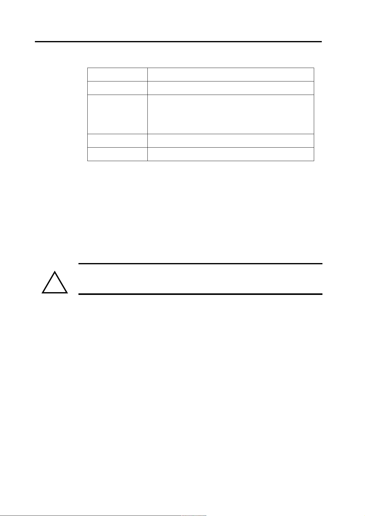
Printing History Neuromag p/n Software Date
1st edition NM20600A 1.3 March 2000
2nd edition NM20600A-A 1.3 May 2004
NM20600A-A 2004-05-17
Page 3

MCE User’s Guide
Contents
1 Introduction . . . . . . . . . . . . . . . . . . . . . . . . . . . . . . . . . . . . . . . . . . . . . . . . . . . . . . . 1
1.1 Hazard Information. . . . . . . . . . . . . . . . . . . . . . . . . . . . . . . . . . . . . . . . . . 1
1.2 Version . . . . . . . . . . . . . . . . . . . . . . . . . . . . . . . . . . . . . . . . . . . . . . . . . . . 2
1.3 What’s new? . . . . . . . . . . . . . . . . . . . . . . . . . . . . . . . . . . . . . . . . . . . . . . . 2
1.4 Conventions and typography . . . . . . . . . . . . . . . . . . . . . . . . . . . . . . . . . . 2
1.5 References. . . . . . . . . . . . . . . . . . . . . . . . . . . . . . . . . . . . . . . . . . . . . . . . . 2
2 Getting Started . . . . . . . . . . . . . . . . . . . . . . . . . . . . . . . . . . . . . . . . . . . . . . . . . . . . . 3
2.1 Analyzing data . . . . . . . . . . . . . . . . . . . . . . . . . . . . . . . . . . . . . . . . . . . . . 3
2.2 Quitting the program. . . . . . . . . . . . . . . . . . . . . . . . . . . . . . . . . . . . . . . . . 3
3 Selecting the data file and pre-processing . . . . . . . . . . . . . . . . . . . . . . . . . . . . . . . 4
3.1 Setting the filtering and baselines . . . . . . . . . . . . . . . . . . . . . . . . . . . . . . . 4
3.2 Decreasing the computing time and file sizes. . . . . . . . . . . . . . . . . . . . . . 5
3.3 Bad channels and projections . . . . . . . . . . . . . . . . . . . . . . . . . . . . . . . . . . 6
4 Selecting the head model . . . . . . . . . . . . . . . . . . . . . . . . . . . . . . . . . . . . . . . . . . . . . 8
4.1 BEM selection. . . . . . . . . . . . . . . . . . . . . . . . . . . . . . . . . . . . . . . . . . . . . . 8
4.2 Point set selection . . . . . . . . . . . . . . . . . . . . . . . . . . . . . . . . . . . . . . . . . . . 9
4.3 Creating BEM files . . . . . . . . . . . . . . . . . . . . . . . . . . . . . . . . . . . . . . . . . 10
5 Calculating the estimates. . . . . . . . . . . . . . . . . . . . . . . . . . . . . . . . . . . . . . . . . . . . 11
6 Loading a calculated estimate. . . . . . . . . . . . . . . . . . . . . . . . . . . . . . . . . . . . . . . . 12
7 Selecting the time . . . . . . . . . . . . . . . . . . . . . . . . . . . . . . . . . . . . . . . . . . . . . . . . . . 13
8 Region of interest . . . . . . . . . . . . . . . . . . . . . . . . . . . . . . . . . . . . . . . . . . . . . . . . . . 14
8.1 What is ROI?. . . . . . . . . . . . . . . . . . . . . . . . . . . . . . . . . . . . . . . . . . . . . . 14
8.2 What is the orientation of a ROI? . . . . . . . . . . . . . . . . . . . . . . . . . . . . . . 14
8.3 Selecting a ROI . . . . . . . . . . . . . . . . . . . . . . . . . . . . . . . . . . . . . . . . . . . . 15
8.4 ROI database. . . . . . . . . . . . . . . . . . . . . . . . . . . . . . . . . . . . . . . . . . . . . . 15
8.5 Exporting ROIs . . . . . . . . . . . . . . . . . . . . . . . . . . . . . . . . . . . . . . . . . . . . 15
9 Predicting MEG waveforms . . . . . . . . . . . . . . . . . . . . . . . . . . . . . . . . . . . . . . . . . 16
10 Printing . . . . . . . . . . . . . . . . . . . . . . . . . . . . . . . . . . . . . . . . . . . . . . . . . . . . . . . . . . 17
10.1 Printing from the dialog . . . . . . . . . . . . . . . . . . . . . . . . . . . . . . . . . . . . . 17
10.2 Saving to an image file . . . . . . . . . . . . . . . . . . . . . . . . . . . . . . . . . . . . . . 17
10.3 Saving with xgifdump command . . . . . . . . . . . . . . . . . . . . . . . . . . . . . . 18
11 Creating HTML documents and MPEG movies. . . . . . . . . . . . . . . . . . . . . . . . . 19
11.1 Creating HTML documents . . . . . . . . . . . . . . . . . . . . . . . . . . . . . . . . . . 19
NM20600A-A 2004-05-17 i
Page 4

MCE User’s Guide
11.2 Creating movies . . . . . . . . . . . . . . . . . . . . . . . . . . . . . . . . . . . . . . . . . . . 20
12 MCE windows and dialogs . . . . . . . . . . . . . . . . . . . . . . . . . . . . . . . . . . . . . . . . . . 21
12.1 Window menus. . . . . . . . . . . . . . . . . . . . . . . . . . . . . . . . . . . . . . . . . . . . 21
12.2 Main window . . . . . . . . . . . . . . . . . . . . . . . . . . . . . . . . . . . . . . . . . . . . . 22
12.3 Pre-processing dialog . . . . . . . . . . . . . . . . . . . . . . . . . . . . . . . . . . . . . . . 23
12.4 MEG data dialog. . . . . . . . . . . . . . . . . . . . . . . . . . . . . . . . . . . . . . . . . . . 26
12.5 Full calculation dialog . . . . . . . . . . . . . . . . . . . . . . . . . . . . . . . . . . . . . . 27
12.6 Batch jobs window . . . . . . . . . . . . . . . . . . . . . . . . . . . . . . . . . . . . . . . . . 28
12.7 Color display . . . . . . . . . . . . . . . . . . . . . . . . . . . . . . . . . . . . . . . . . . . . . 29
12.8 Arrow display . . . . . . . . . . . . . . . . . . . . . . . . . . . . . . . . . . . . . . . . . . . . . 30
12.9 Amplitude window . . . . . . . . . . . . . . . . . . . . . . . . . . . . . . . . . . . . . . . . . 31
12.10 Amplitude scale window . . . . . . . . . . . . . . . . . . . . . . . . . . . . . . . . . . . . 32
12.11 Color scale window . . . . . . . . . . . . . . . . . . . . . . . . . . . . . . . . . . . . . . . . 33
12.12 Region of interest window . . . . . . . . . . . . . . . . . . . . . . . . . . . . . . . . . . . 34
12.13 ROI database window. . . . . . . . . . . . . . . . . . . . . . . . . . . . . . . . . . . . . . . 35
12.14 HTML Creation Dialog . . . . . . . . . . . . . . . . . . . . . . . . . . . . . . . . . . . . . 38
12.15 Movie Creation Dialog. . . . . . . . . . . . . . . . . . . . . . . . . . . . . . . . . . . . . . 39
Index . . . . . . . . . . . . . . . . . . . . . . . . . . . . . . . . . . . . . . . . . . . . . . . . . . . . . . . . . . . . 41
ii 2004-05-17 NM20600A-A
Page 5

MCE User’s Guide Introduction
1 Introduction
This manual describes the use of MCE program to analyze magnetoencephalo-
graphic (MEG) measurements using L1 minimum norm estimates
1.1 Hazard Information
This manual contains important hazard information which must be read, understood and observed by all users, For your convenience all warnings that appear
in the manual are presented below.
Warning: Like all inverse solutions of MEG, MCE provides a source
distribution which is one of infinitely many different possible ones. The results
!
must be interpreted and reviewed by a person having good understanding of the
capabilities and limitations of the methods being used.
1,2
(L1 MNE).
Warning: This program should only be used with hardware and software given
!
!
!
!
!
in the specifications listed in the Release Notes of the release being used.
Warning: On some platforms other programs can affect the colors in the
windows of the MCE program. In such cases other programs using colored
windows should be stopped to ensure correct colors on the displays.
Warning: The triangle meshes used in MCE to describe the shape of the brain
must be defined in head coordinates. This differs from the recommended
coordinate system usage in dipole modeling program.
Warning: If the regularization parameters are changed from the default ones,
the new values must be validated using known data.
Warning: Region of interest may contain multiple sources whose activities are
mixed together.
Warning: All users that have access to the database can also access the data-
!
NM20600A-A 2004-05-17 1
base entries related to the data of other users.
Page 6

Introduction MCE User’s Guide
1.2 Version
This manual refers to program version 1.3 patch level 18 and later.
1.3 What’s new?
• Default directory menu
• Export figure menu
• Batch calculation error log display
• Slowed down animation
• Calculation can be cancelled
• Showing selected ROI in arrow display
• Show subject ID & file name in different figures
• Added several warnings to the manual
1.4 Conventions and typography
Buttons that can be pressed will be shown in square brackets: [Button]
Text written by the user is shown as
User input
Some important warnings are shown in bold.
1.5 References
1. K. Matsuura and U. Okabe, “Selective minimum-norm solution of the
biomagnetic inverse problem”, IEEE Trans. Biomed. Eng. 42:608-615, 1995.
2. K. Uutela, M. Hämäläinen, and E. Somersalo, “Visualization of
Magnetoencephalographic Data using Minimum Current Estimates”,
NeuroImage, 1999. In press.
2 2004-05-17 NM20600A-A
Page 7
MCE User’s Guide Getting Started
2 Getting Started
To start the program, double click the MCE icon in the Neuromag folder of the
Application manager. An iconified Matlab console appears on the desktop;
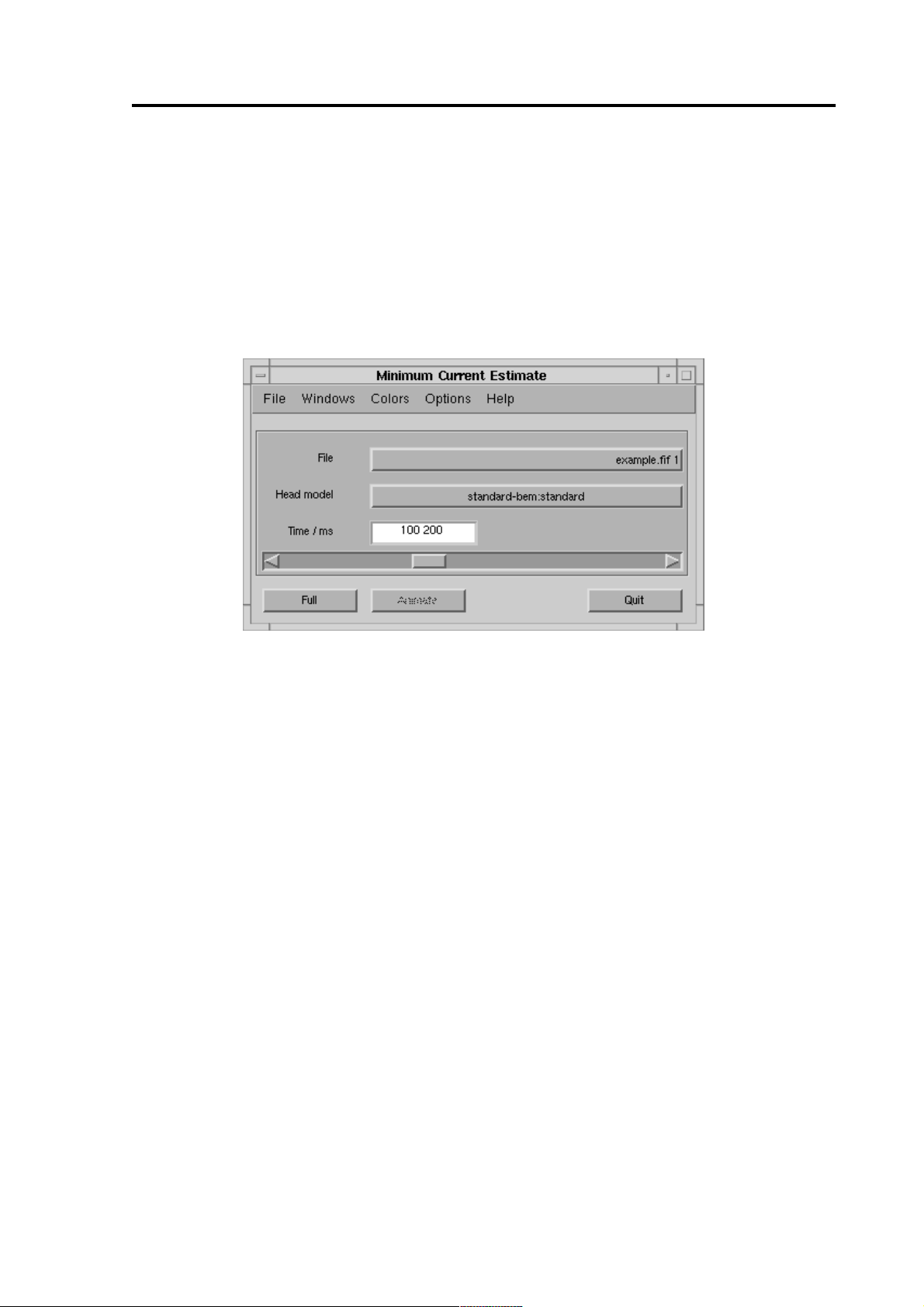
do not close it! Also the main window shown in Figure 1 opens.
If you are using a previously calculated response, you should now load an old
calculation (p. 12). Otherwise, you should select a data file using the [File] but-
ton and select the head model (p. 8). The main window is described in more
detail on page 22.
Figure 1 The main window
2.1 Analyzing data
To analyze your data with the L1 MNE, first you should calculate the estimates:
1. Load and pre-process the MEG data (p. 4)
2. Select the head model (p. 8)
3. Start the calculation (p. 11)
After you have loaded (p. 12) the calculated estimates, you can proceed by
viewing the results (p. 33) at different times (p. 13) or by studying the temporal
activity of the Regions of Interest (p. 14).
2.2 Quitting the program
You can quit the program by three alternative ways:
1. pressing the [Quit] button in the Main window
2. typing “quit” Matlab command in the terminal window
3. by closing the main window.
NM20600A-A 2004-05-17 3
Page 8
Selecting the data file and pre-processing MCE User’s Guide
3 Selecting the data file and pre-processing
Select the MEG data file by pressing the [File] button of main window (p. 22).
Select the data file from the dialog. If the file has several data sets, a selection dialog pops up and you can select the correct data set.
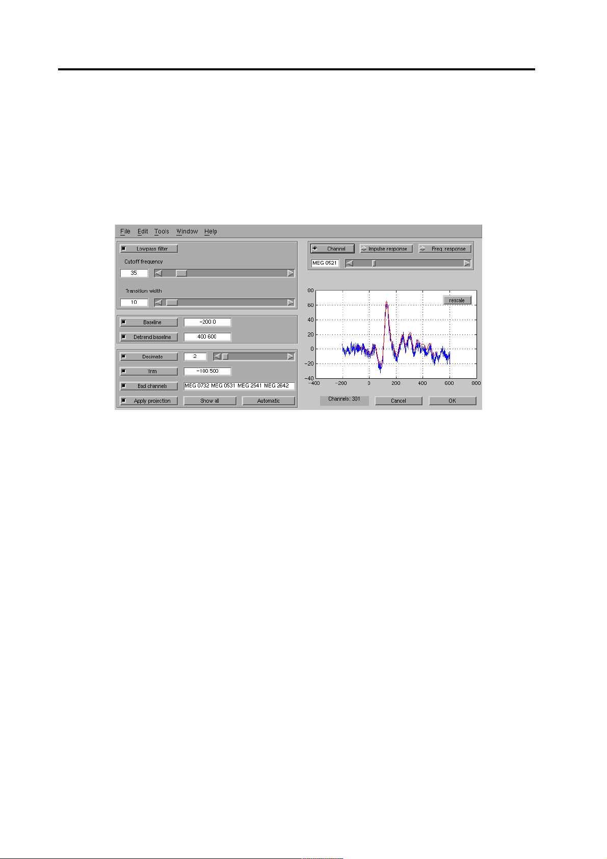
When the you have selected the data, the pre-processing dialog (see Figure 2) will
open.
Figure 2 The pre-processing dialog
3.1 Setting the filtering and baselines
Because the MEG signals are mainly concentrated to the lower frequencies, you
can increase the signal-to-noise ratio with an low-pass filter. Select the [Lowpass
filter] toggle and set appropriate cutoff frequency and transition width of the filter.
After changing the numeric values, press Enter or the Tab key to update the value.
You can view the effect on a single channel by pressing the [Channel] toggle or
the filter response with the [Impulse response] and [Freq. response] buttons.
You can zoom into the preview window with the left mouse button and revert to
automatic scaling with the [rescale] button.
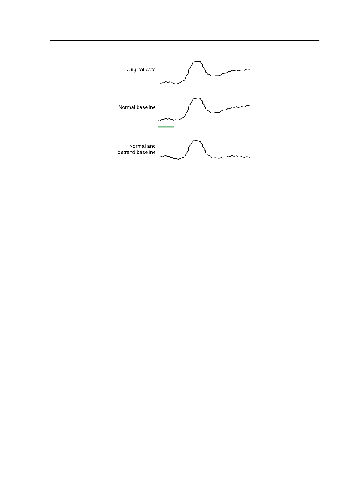
Because most of the channels usually have a non-zero DC-level, you should select
a [Baseline] toggle and select a time period where there should be no real evoked
responses, typically before the stimulus.
If you are analyzing a long period or the data otherwise includes strong artificial
slow drifts, you can select a [Detrend baseline] period after the evoked response.
This is usually a safer way of getting rid of the drifts than, for example, applying
high-pass filter.
The de-trend baseline actually fits a line to the values in the two baselines and subtracts it form the data (see Figure 3).
4 2004-05-17 NM20600A-A
Page 9
MCE User’s Guide Selecting the data file and pre-processing
Figure 3 Effect of the baselines
3.2 Decreasing the computing time and file sizes
If you do not calculate estimates at all the time points, you can decrease the
computing time and save disk space.
If you low-pass filter the data, the data will be smoother and it is unnecessary to
calculate the estimate at each time point. By selecting a down-sampling ratio
with the [Decimate] toggle and slider, the estimates will be calculated with
constant intervals.
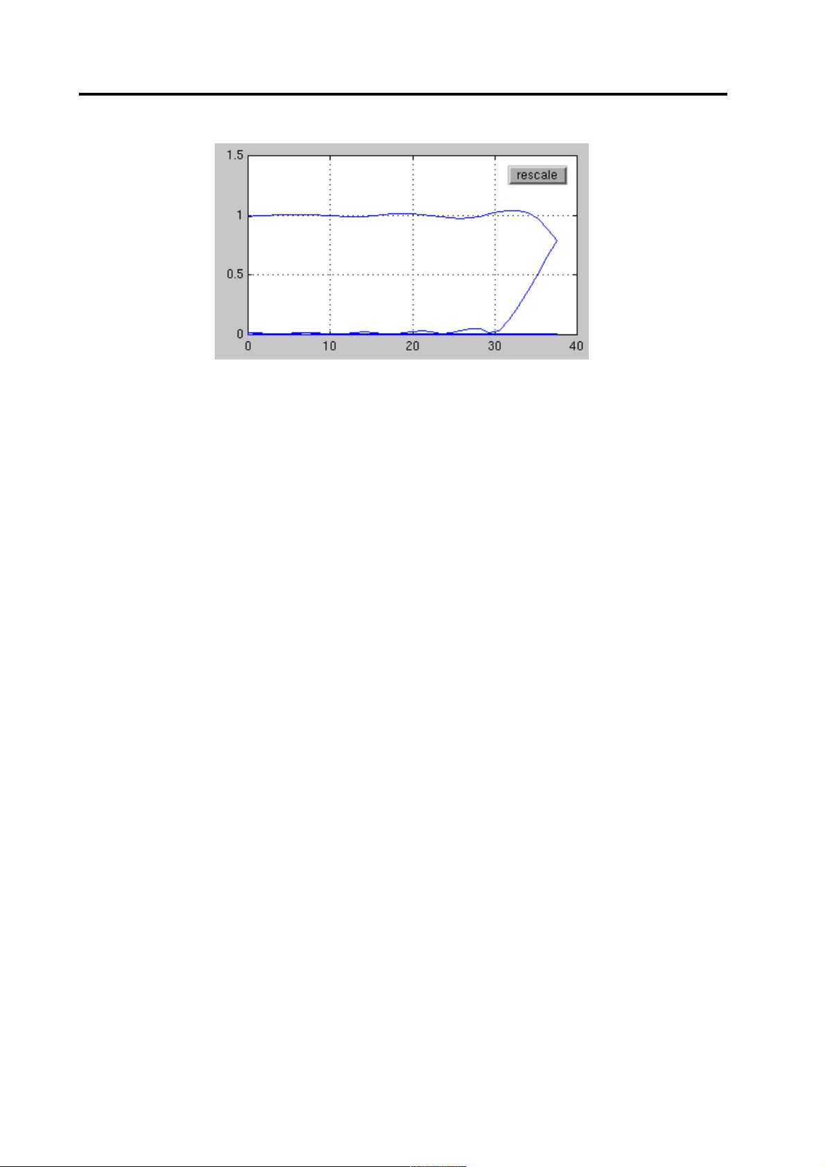
You can select the correct amount of down-sampling by selecting the [Freq.
response] button. If the down-sampling is too strong compared to the filter
pass-band, the higher frequencies will be mapped to the lower frequencies (see
Figure 4). A reasonable down-sampling ratio is the one, for example, having the
cutoff frequency about half way between the zero frequency and the highest
shown frequency. The down-sampling is carried out by selecting single data
points of the filtered response.
If you do not need to analyze the whole epoch, select the interesting time period
with the [Trim] toggle button and text fields.
NM20600A-A 2004-05-17 5
Page 10
Selecting the data file and pre-processing MCE User’s Guide
Figure 4 If too strong down-sampling is applied, the aliasing is reflected in the
preview window with the folding frequency response. Decrease the filter cutoff
frequency or decimation.
3.3 Bad channels and projections
If some of the channels are flat or bad, you must set the [Badchannels] toggle and
write the channel names to the corresponding text field. The format can be “MEG
1112 1113 ...” or “MEG 1112 MEG 1113 ...”, the channels described with
four digits for Elekta Neuromag™ or Vectorview™ data and three digits for Neuromag-122™ data. Use the numbers in the channel names regardless of the channel
order in the fif-file. Wildcards are not supported.
External disturbance fields can be filtered using Signal Space Projection (SSP). If
the fif-datafile has a noise projection specified, you can apply it to the data and cal-
culations by selecting the [Apply projection] toggle. The projection is updated
when you change the bad channels. Normal data files where the projection information is included and the data itself is the original non-projected data should be
used. If projected data is used, the file must also contain the projection vectors that
were used define the removed subspace. Otherwise the results may be distorted.
When you load a new file or press the [Automatic]button, the bad channels are set
automatically. The following channels are set bad:
1. Channels that are marked bad in the fif-file
2. If baseline is used, the channels where the baseline is flat
3. If baseline is used, the channels where the baseline is very noisy
The “flat channels” are the ones where the standard deviation of the raw baseline
activity is less than 10 % of the median value of others. The “noisy channels” are
the ones where the standard deviation of the baseline activity after projections is
over three times the median value. If the data includes both gradiometer and magnetometer data, the values are only compared with the channels with same coil
type.
6 2004-05-17 NM20600A-A
Page 11

MCE User’s Guide Selecting the data file and pre-processing
In practice, you should first specify the baseline period and then press the
[Automatic] button, and then add bad channels that are not included. Because
the selection of the bad channels slightly affects the projections and the projections affect the selection of the noisy channels, resetting the projections repeatedly may result in different channels being marked bad at the second time, if
their noise levels are near the limits.
A handy way of screening for possible bad channels is to open the MEG Data
dialog (p. 26) by pressing the [Showall] button. All the channels will be shown,
overlaid based on the location. If one of the waveforms seems to be an outlier,
right-click it at the time of the maximum difference, and the channel ID is
shown.
NM20600A-A 2004-05-17 7
Page 12
Selecting the head model MCE User’s Guide
4 Selecting the head model
You can select the head model by pressing the [Head model] button in the Main
window (p. 22). The head model consists of two parts: the boundary element
model (BEM) (p. 8) describes the shape of the brain and the point set (p. 9)
describes the parameters needed in the calculation. First, the BEM model selection
window opens up.
4.1 BEM selection
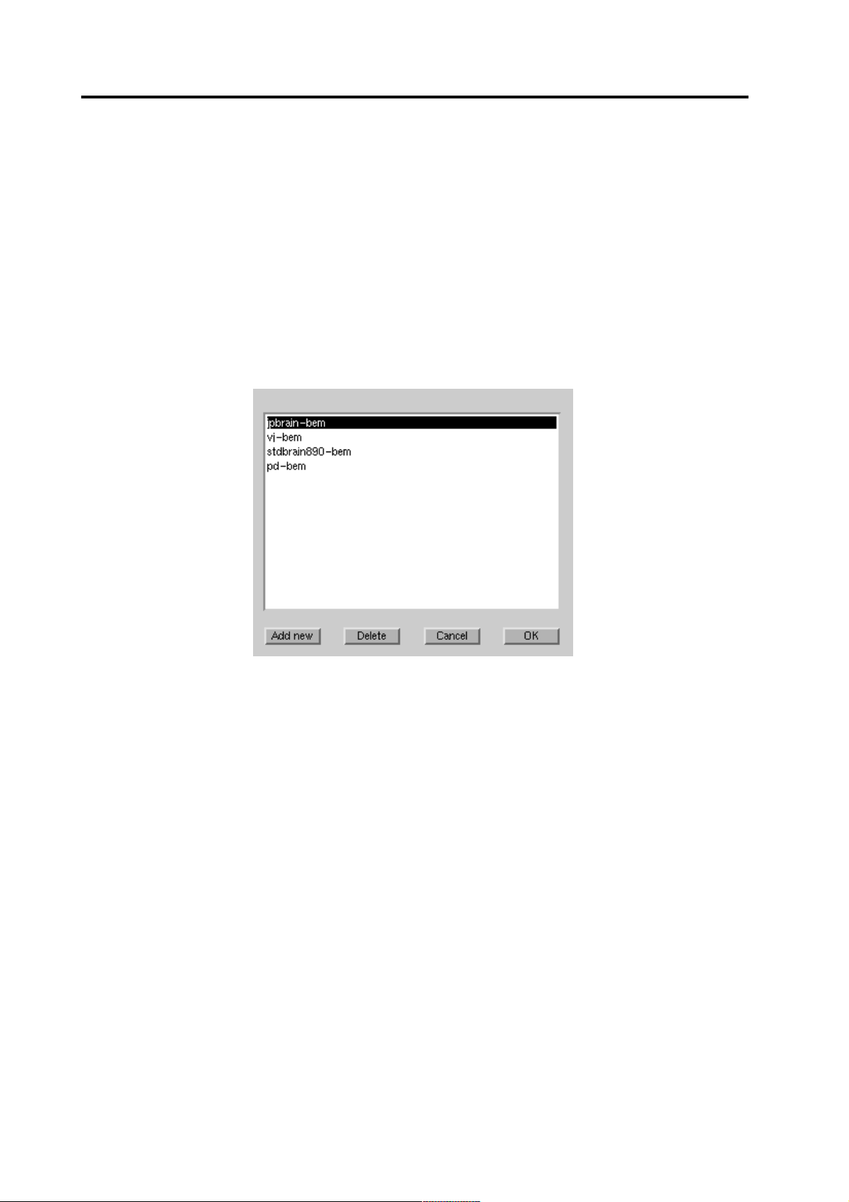
Figure 5 BEM model selection dialog
The boundary element model (BEM) describes the shape of the brain. In the current version (1.3), only sphere models are used in the forward calculation, but the
BEM model affects the point set used in the calculation and the images used in the
3D visualization.
The BEM dialog shows a list of existing models associated with the same subject
and some general models. You can select an existing model from the list and accept
it by pressing the [OK] button.
You can add a new BEM model by pressing the [Add new]button. A file selection
box for selecting the fif-file opens up, and after the selection you can select the
associated the subject.
If the BEM model is not used by any point set (p. 9), you can delete it by pressing
the [Delete] button. If it is used by point sets, you should first delete the point sets.
After you have accepted the BEM model by pressing the [OK] button, you should
select the point set.
8 2004-05-17 NM20600A-A
Page 13
MCE User’s Guide Selecting the head model
4.2 Point set selection
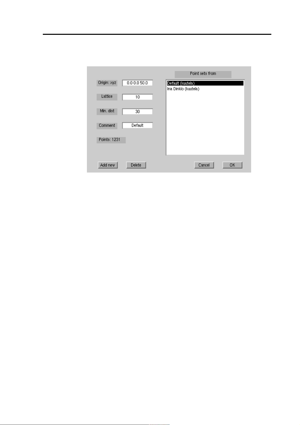
Figure 6 Point set selection dialog
The point set includes the brain locations that are used as a source space in the
calculations and the parameters of the conductor model used in the forward calculations. Each point set is related with a certain BEM model (p. 8) and a certain subject.
From the Point set dialog you can select an existing set from the list and accept
it by pressing the [OK] button. After this you can proceed by making the full
calculation (p. 11).
You can create a new point set by pressing the [Add new] button and setting
appropriate values to the properties of the point set. If you modify the Origin,
Lattice, or Min dist properties, the point set is recalculated and the number of
points is show. If you accept the new point set by pressing the OK button, it will
take a while to calculate the projection from the point set to the BEM. You can
remove the point sets by pressing the [Delete] button. If several people are
using the point set, it will be deleted only when it is deleted by all its users.
NM20600A-A 2004-05-17 9
Page 14
Selecting the head model MCE User’s Guide
Table 1 Properties of the point sets
Origin: xyz Sphere model origin (in mm; head coordinates)
Lattice The density of the points in the point set (in mm)
Min dist The minimum distance to the sphere model origin (in
mm). Points deeper than this are excluded from the
point set. Very deep source points may lead to numerical instability in the calculations.
Comment The comment seen in the list
Points The number of possible source points
4.3 Creating BEM files
If you have MR images of the subject, you can create fif-files describing boundary
element models of the brain with MriLab and meshes2fiff programs. See the manuals of those programs (or Source Modeling manual) for details of using those programs.
When creating the meshes in Mrilab, you must save them in head coordinates
in meters.
Warning: The triangle meshes used in MCE to describe the shape of the brain
must be defined in head coordinates. This differs from the recommended coordi-
!
nate system usage in dipole modeling program.
10 2004-05-17 NM20600A-A
Page 15

MCE User’s Guide Calculating the estimates
5 Calculating the estimates
Before viewing the results you have to calculate the current estimates for the
epoch.
You should have already selected the MEG data, pre-processed it, and selected
the head model (see chapters “Selecting the data file and pre-processing” on
page 4 and “Selecting the head model” on page 8). If the noise level of the measurement is very high or low, you might change the regularization level or if
either magnetometers or gradiometers are especially noisy their relative noise
levels (p. 22).
Add the current data set by pressing the [Full] button in the main window (p.
22). The full calculation dialog opens up. Check that the [Calculate] button is
pressed and press the [OK] to add the new batch job.
Now the batch jobs window (p. 28) opens up. The job you just created is in the
list in the wait state. The preferred way of calculating the estimates is to press
the [Start server] button. This will start the calculation in the background. The
server selects the job whose priority order is smallest and calculates the esti-
mate. When it has finished, it saves the results to a file with name like file-
name#_full.mat, where filename is the name of the data file and # is the
number of the data set, selects a new job and continues calculating that. When
there are no more jobs waiting, the server quits.
Note: The server uses a separate Matlab program which may require an additional Matlab license to run.
If there is an error in the calculation, the job is left on the list, but its state
changes to err. This may happen, for example, if the computer where the
server runs can not access the data files. When the server quits, it writes a log
file. You can view the latest error log file created by the server with the [Error
log] button. You calculate the estimate by resetting the job (p. 28) and starting a
new server in a computer that can access the data file. You can have only one
server in one computer. You can start the calculation server in other computers
also by giving the UNIX command
/neuro/mce/settings/l1calc
When the server is running, you can use the main program to add new jobs or
view the results, or even quit the program and free the terminal for others.After
the estimate has been calculated, you should load it with the [Full] button.
Another method to start the calculation is to select one particular job and press
the [Calculate] button. You will see the progress bars, but you can not use the
program for other tasks, and quitting the application cancels the calculation.
You can also cancel the calculation by pressing any button in the Batch calculation window. In this case the calculated estimate is loaded automatically. The
error log is not updated; instead, the possible error messages are shown in the
Matlab command window.
NM20600A-A 2004-05-17 11
Page 16

Loading a calculated estimate MCE User’s Guide
6 Loading a calculated estimate
If you have previously calculated (p. 11) an estimate and saved it to a disk file, you
can load it by pressing the [Full]button in the Main window (p. 22) to open the full
calculation dialog (p. 27).
If you have selected the right fif-file and have previously saved the corresponding
estimate with the default name, the default values in the dialog should be set to
load the estimate.
Otherwise, check that the [Load] button in the Full calculation dialog (p. 27) is
pressed and select the estimate with the [Select file...] button.
When you press the [OK] button, the batch calculation and its parameters are
loaded.
The program can also load estimates calculated previous versions of the program,
but some features are not available. For example, the subject ID may be incorrect.
12 2004-05-17 NM20600A-A
Page 17

MCE User’s Guide Selecting the time
7 Selecting the time
You can select a single time point in three ways:
• By entering the time (in ms) in the [Time] field in the Main window (p. 22).
• By using the slider in the Main window (p. 22).
• By pressing the left mouse button in the Amplitude window (p. 31), if a
batch calculation is loaded.
However, because the single estimates are usually noisy, it is usually more
fruitful to view the average activity within a time range. You can also select the
range in three ways:
• By entering the start and end time (in ms) in the [Time] field in the Main
window
• By pressing the and dragging with the right mouse button in the Amplitude
window (p. 31)
• By giving in the Matlab terminal window command
startl1('span',tmin:tmax)
where tmin and tmin are the start and end times in milliseconds. For
example, to select time span between 100 and 200 milliseconds, use
startl1('span',100:200)
NM20600A-A 2004-05-17 13
Page 18

Region of interest MCE User’s Guide
8 Region of interest
You can estimate the activity in certain brain area as a function of time by defining
a region of interest (ROI). ROI is actually a weighting function that is used to calculate the sum amplitude from the estimate.
8.1 What is ROI?
The smoothed weighting is a function of position r, having form
fr() e
but you don't need to be interested in matrix calculation to understand how the
ROIs work.
The ROI window (p. 34) visualizes the currently selected ROI with an ellipsoid.
The weight in the center has weight 1 in the sum, and the points on border of the
ellipsoid have the weight 0.60.
Activity at each source location is multiplied with the corresponding weight and
added together. The weighted sum is shown in the Amplitude window (p. 31).
A ROI can also have hard edges. In this case, the weight is
fr() 1=
If no ROI is selected, normal sum of all the activity is used.
8.2 What is the orientation of a ROI?
T
r
=
, if , otherwise 0.
Wr–
T
r
Wr– 1<
Since MEG is sensitive to the orientation of the neural currents and this information is often very useful in differentiating nearby source areas, the ROIs can be
used with a defined orientation. The weighting function depends in this case also
on the orientation
q0 and the direction of the estimated current q:
⋅
qq
0
grq,()fr()
=
------------------
qq
0
The amplitude is the projection of the estimated current on the selected orientation.
If the estimated current is parallel with the ROI, the amplitude will be the same as
for the non-oriented ROI. If the orientation is opposite, the amplitude will be negative. You can select to use either the oriented or non-oriented ROI with the Amplitude scale window (p. 32).
14 2004-05-17 NM20600A-A
Page 19

MCE User’s Guide Region of interest
8.3 Selecting a ROI
You can select a ROI from the Color display (p. 29). Select a range of nodes
with the right mouse button.
The program will find the active source points that are contributing to the
selected activity and calculate the ROI center and extent. The orientation of the
ROI will be the mean orientation of selected currents.
After selecting a new ROI, activity weighted with it is shown in the ROI window (p. 34), the time course of activity in the area is shown in the Amplitude
window (p. 31), and the parameters of the ROI are shown in the ROI database
(p. 35). In the Color display or Arrow display (p. 30) you can toggle between
showing the selected activity and all the activity by pressing any key when the
window is selected.
Warning: Region of interest may contain multiple sources whose activities are
!
mixed together.
8.4 ROI database
You can compare the activity of a certain brain area in different measurements
and subjects by saving the ROIs in a database.
You can access the database with the ROI database window (p. 35). When you
have selected the ROI corresponding to the interesting brain area, write the
name of the area in the [Comment] field and press the [Save] button.
If you want to see the activity of the same area during another measurement,
load (p. 12) the corresponding estimate, press down the [Show other files] but-
ton, and select the area from the list.
If you compare the results of different subjects and possibly with your col-
leagues, you may need to press down the [Show other subjects] button or
change the user name in the [Creator]field. If there is a huge number of ROIs in
the database, you can constrain the search using SQL search (p. 37).
8.5 Exporting ROIs
You can export the ROI ellipsoids to Mrilab with the [Export new file] and
[Append] commands in the [Options] menu of the ROI database window (p.
38). The output files can be imported to Mrilab (see corresponding manual for
details).
NM20600A-A 2004-05-17 15
Page 20

Predicting MEG waveforms MCE User’s Guide
9 Predicting MEG waveforms
Figure 7 Predicted fields shown with XPlotter. The original measurement is
shown with yellow lines and the waveforms predicted with the activity of the
selected ROI is shown with red lines.
To find out, what part of the measured data is explained with the activity in the
selected ROI, you can press the [Show predicted fields] command in the
[Options] menu of the Amplitude window (p. 31). The program calculates the
magnetic field produced by the currents in the selected ROI and shows them with
the XPlotter program together with the original data loaded from the fif-file. If you
select a new ROI, the waveforms are updated when you select the [Show pre-
dicted fields] button again.
16 2004-05-17 NM20600A-A
Page 21

MCE User’s Guide Printing
10 Printing
You can print the displays or save them as images by using the printing dialog,
or with UNIX command
/neuro/mce/bin/xgifdump
10.1 Printing from the dialog
Figure 8 The printing dialog
The [Print] command in the File menu (p. 21) opens the printing dialog. Select
the correct paper type and orientation, select the correct printer by typing
-Pprintername -dpsc2
in the [Device option] field and press the [Print] button.
10.2 Saving to an image file
The [Print] command in the File menu (p. 21) opens the printing dialog. You
can save the image with a format compatible with old Adobe Illustrator by typing
-dill
in the [Device option] field, or as a general EPS-file (which can be opened in
Adobe Illustrator version 6 or newer) with the option
-depsc
To produce JPEG output, use the option
-djpeg
Press down the [File] button, then the [Save...] button, and a dialog for the out-
put file name is opened.
NM20600A-A 2004-05-17 17
Page 22

Printing MCE User’s Guide
The EPS formats suit well the Arrow (p. 30), Amplitude (p. 31), and Region of
interest (p. 34) windows. In the conversion of the color displays (Color display (p.
29), Color scale (p. 33)) some errors may occur; the JPEG or PNG formats are
more suitable for them.
10.3 Saving with xgifdump command
The images can be saved in GIF format by giving the command
/neuro/mce/bin/xgifdump
in an UNIX terminal window.
The command will ask the name of the output file and to select the correct window
with the mouse. A convenient way to save several images from the Color display
(p. 29) is to create an HTML file (p. 19), which includes the images in PNG format.
18 2004-05-17 NM20600A-A
Page 23

MCE User’s Guide Creating HTML documents and MPEG movies
11 Creating HTML documents and MPEG movies
11.1 Creating HTML documents
Figure 9 An example of a created HTML document
You can create HTML documents with the HTML document creation dialog (p.
38). The document will include projected, color coded views of the estimate
from selected orientations and different time periods. The images in PNG (Portable Network Graphics) format are saved in the same folder as the HTML file,
with names like prefix_begintime_endtime_orientation.png.
You can view the results with typical HTML browsers, such as Netscape Navigator™ or Microsoft’s Internet Explorer™.
NM20600A-A 2004-05-17 19
Page 24

Creating HTML documents and MPEG movies MCE User’s Guide
Table 2 Default viewing orientations for created HTML documents MPEG
movies
11.2 Creating movies
Orientation Horizontal
Elevation
rotation
left -90 0
right 90 0
back 0 0
top 0 90
bottom 0 -90
front 180 0
upleft -90 30
upright 90 30
leftback -45 30
rightback 45 30
You can create MPEG movies with the Movie creation dialog (p. 39). The movie
will show projected, color coded views of the estimate from the selected orientation. To smoothen the animation, each movie frame will represent the average
activity during specified time window. If you want the best possible temporal resolution, set the window length to the frame skip length, otherwise use longer window lengths. You should be able to view the produced MPEG-1 movie with most
common MPEG movie viewing programs. A public domain MPEG viewing program by The Regents of the University of California can be used with the UNIX
command
/neuro/mce/bin/mpeg_play movie.mpeg
20 2004-05-17 NM20600A-A
Page 25

MCE User’s Guide MCE windows and dialogs
12 MCE windows and dialogs
12.1 Window menus
Figure 10 Menus of the Main Window (p. 22)
File
Create HTML ... Opens the HTML creation dialog (p. 38)
Create movie ... Opens the HTML creation dialog (p. 39)
Print... Opens the print dialog (see Printing (p. 17))
Close Closes the current window
Windows
Opens the different windows
Colors
Selects the color map for current window
Help
L1 MNE Help Opens this manual in a Web browser
About L1 MNE Shows the version
Options
Some windows have specific options.
NM20600A-A 2004-05-17 21
Page 26

MCE windows and dialogs MCE User’s Guide
12.2 Main window
Figure 11 The main window
The main window is opened when the program starts, and closing it quits the program.
Table 3 Controls in the Main window
[File] Select the name of the fif-file containing the response.
Shows the name of the selected file. If a batch calcula-
tion is loaded, has the text (full) behind the file
name.
[Head model] Select the head model (p. 8). Shows the currently
selected BEM (p. 8) and point set (p. 9).
[Time] The slider and text field select and show the current
time range (p. 13).
[Full] Opens the full calculation dialog (p. 27).
[Animate] Starts an animation in the Color display (p. 29) from
the current time point. The animation can be stopped
by pressing the same button.
[Quit] Quits (p. 3) the MCE program.
Options menu
The [Options] menu in the main window includes buttons [MNE options], [Preprocessing], and [Batch tasks] buttons. The [MNE options] button opens the
MNE Options window.
22 2004-05-17 NM20600A-A
Page 27

MCE User’s Guide MCE windows and dialogs
Figure 12 Minimum norm estimate options dialog
The [Regularization] slider and text field select and show the number of singu-
lar values of the data used in the estimate. If the noise level in the measurement
is low, increase the value to correctly estimate more complex source distributions. If the noise level is high, decrease its effect by decreasing the value. The
default value (30) is usually reasonable for averaged evoked responses.
Keeping the [Depth normalization] button pressed compensates for the ten-
dency of the estimate to produce too superficial sources.
The Elekta Neuromag™ and Vectorview™ have both magnetometer and gradiometer sensors. In the estimation, the signals are analyzed in relation to the
noise level. The default values (5 fT/cm for gradiometers, 25 fT for magnetometers) are reasonable in evoked response measurements, but if for some reason
their relative noise level changes, you can modify the values in this dialog. Press
the [Set noise levels manually] button and change the values in the text fields.
If the options are changed, the windows displaying the previous estimate are
closed.
Warning: If the regularization parameters are changed from the default ones,
!
the new values must be validated using known data.
12.3 Pre-processing dialog
The pre-processing dialog is opened by pressing the [Preprocessing] button in
the Options menu or automatically when you select a new data file.
NM20600A-A 2004-05-17 23
Page 28

MCE windows and dialogs MCE User’s Guide
Figure 13 The pre-processing dialog
The left side of the window shows controls that you can use to pre-process the data.
With the filter frame you can low-pass filter the data, with the baseline frame you
can compensate for the DC level and slow drifts. With the projection frame you can
down-sample the data and select the interesting period for the calculation. and set
bad channels and noise projection.
The right side of the window shows a preview of the original data (blue) and processed data (blue). You can zoom into the display with the left mouse button. The
preview frame lets you either select the channel or to view the amplitude or frequency response of the filter. The latter can be used to check for a good down-sam-
pling ration; the [Rescale] button reverts to automatic scaling.
See chapter “Selecting the data file and pre-processing” on page 4 for additional
instructions using this dialog.
24 2004-05-17 NM20600A-A
Page 29

MCE User’s Guide MCE windows and dialogs
Table 4 Controls in the Pre-processing dialog
Filter frame The [Lowpass filter] toggle selects the filter. You can
select the cutoff frequency or transition width with the
corresponding text fields or sliders.The values are in Hz.
Use the [Freq. response] and [Impulseresponse] but-
tons to see the effect of the filter.
Units: Hz
Baseline frame The [Baseline] toggle and the corresponding text field
select the baseline period used to remove the DC offset
and in automatic selection of the bad channels (p. 4).
The [Detrend baseline] toggle and the corresponding
text field select the other baseline used for removing
slow drifts (p. 4).
Units: ms
[Decimate] The toggle button and text field or slider select the
down-sampling ratio. See section “Decreasing the computing time and file sizes” on page 5.
Units: samples
[Trim] The toggle button and text field select the analysis
period.
Units: ms
[Bad channels] The toggle button and text field set the bad channels.
Write the channel numbers to the text field with format
‘MEG #### #### #### ####’
[Apply projection] If the toggle button is set, the noise projection defined in
the data file is applied to the data and calculations.
[Show all] Opens the MEG data -dialog (p. 26).
[Automatic] The button resets the projection and bad channels to
default values. See “Bad channels and projections” on
page 6.
Preview frame The buttons let you select either a single channel or filter
properties in the preview plot
Preview plot Shows the selected information; original data in red and
processed data in blue. Left mouse button zooms in the
image, the [rescale] button reverts to automatic scaling.
X-axis units: ms in Channel and Impulse response
mode, Hz in freq. response mode.
Y-axis units: fT for magnetometers, fT/cm for gradiometers.
[Cancel] Closes the window
[OK] Applies the new values and closes the window
NM20600A-A 2004-05-17 25
Page 30

MCE windows and dialogs MCE User’s Guide
12.4 MEG data dialog
The MEG data dialog is opened with the [Show all] button of the Pre-processing
dialog (p. 23). It shows waveforms of all the channels overlaid based location.
Left-clicking zooms in the image, right-clicking shows the maximum amplitude
and channel in the selected time and location. The commands in the [Options]
menu (p. 26) can be used to set the scale and layout.
Table 5 Commands in the Options menu of the MEG data dialog
[Channels] Opens Meg channels window for selecting the shown
channels and scaling
[Selections] Opens Channel selection window for selecting pre-
defined layouts
[Groups] Opens Channel group window for selecting grouping of
channels in the layout
[Remove mean] Removes the mean value of the waveforms
26 2004-05-17 NM20600A-A
Page 31

MCE User’s Guide MCE windows and dialogs
12.5 Full calculation dialog
Figure 14 The full calculation dialog
The full calculation dialog is opened by pressing the [Full] button in the Main
window (p. 22).
This window is used to calculate (p. 11) or load (p. 12) the minimum norm estimates of a whole response. The calculation of a new estimate will take will take
some time, typically a second or two for each time point in the response.
Table 6 Controls in the full calculation dialog
[Calculate] This button should be pressed if you want to calculate
a new estimate
[Load] This button should be pressed if you want to load an
old estimate
[Select file ...] Use the large button to select the file name of the
saved or loaded estimate. If a fif-file is selected, this
button shows the default name of the batch file.
NM20600A-A 2004-05-17 27
Page 32

MCE windows and dialogs MCE User’s Guide
12.6 Batch jobs window
Figure 15 The batch jobs window
This window controls the calculation of the estimates. The list shows current batch
jobs and their states. The preferred way to start a calculating all the jobs, press the
[Start server] button. This will be done in the background and you can use the
program to add new jobs or view the results, or even log out and free the terminal
for others. You can update the list by clicking it with mouse button.
You can also select one particular job and press the [Calculate] button. to see the
progress bars, but then you can not use the program for other tasks and you must
not log out before the calculation is finished. See “Calculating the estimates” on
page 11.
Table 7 Controls in the batch jobs window
[Calculation] Start calculating the selected job. You will see progress
of the calculation, but you can not use the program
[Priority] Set the priority of the selected job
[Delete] Delete the selected job
[Reset] Reset the job after an error or stop calculating it
[Details] Show details of the selected job
[Start server] Start a calculation in the background
[Stop server] Stop the calculation in the background
[Close] Close the window
28 2004-05-17 NM20600A-A
Page 33

MCE User’s Guide MCE windows and dialogs
12.7 Color display
Figure 16 Color display of the estimate
The color display is opened by selecting [Color display] in the Windows menu
(p. 21).
The color display shows the estimated source distribution projected to the surface of the brain. The projection is done along the radius of the sphere model. If
a time period is selected, the average activity during the period is shown.
You can rotate the image by moving the mouse while holding down the left button. The color scale can be viewed and changed with the Color scale window (p.
33). The coloring of the window can be changed with the [Colors] menu.
You can select a region of interest (ROI, “Region of interest” on page 14) by
pressing down the right mouse button and dragging over the active area. The
color display will show the selected activity only. You can toggle between
showing the selected or all activity by using [Selected] button in the [Options]
menu or by pressing space bar while the window is active.
You can view the location of the peak activity by selecting [Max] in the
[Options] menu
NM20600A-A 2004-05-17 29
Page 34

MCE windows and dialogs MCE User’s Guide
12.8 Arrow display
Figure 17 Arrow display of the estimate
The arrow display is opened by selecting [Arrow display] in the Windows menu
(p. 21).
The arrow display shows the 3-dimensional estimated source locations and orientations. If a time period is selected, the average activity during the period is shown.
You can toggle between showing the selected or all activity by using [Selected]
button in the [Options] menu or by pressing space bar while the window is active.
You can rotate the image by moving the mouse while holding down the left button.
The arrow length and colors are automatically scaled and the colors are not comparable with the Color scale window (p. 33). The coloring of the arrows can be
changed with the [Colors] menu.
30 2004-05-17 NM20600A-A
Page 35

MCE User’s Guide MCE windows and dialogs
12.9 Amplitude window
Figure 18 The amplitude window with total activity
Figure 19 The amplitude window with an oriented ROI
The amplitude window is opened by selecting [Amplitude] in the Windows
menu (p. 21).
NM20600A-A 2004-05-17 31
Page 36

MCE windows and dialogs MCE User’s Guide
The amplitude window shows the activity of the selected ROI (p. 14) during the
whole response. You can also use it to select a time point or time range (p. 13).
To select a time point, use the left mouse button. To select a time range, drag with
the right mouse button.
The text box shows the selected ROI, time range and the average amplitude during
the time range.
You can change the X- and Y-axis scales, or toggle using the orientation of the
ROI, with the amplitude scale window (p. 32).
The [Option] menu includes the button [Show predicted fields], which shows the
measured and predicted MEG waveforms with the XPlotter program (p. 16).
12.10 Amplitude scale window
Figure 20 Amplitude scale window
With the amplitude scale window you can set the scale of the X- and Y-axes of the
amplitude window (p. 31). The [Auto] toggle button selects automatic or manual
scaling. In the manual scaling mode you can define the minimum and maximum
values in the corresponding text field. The X-axis units are ms and Y-axis units
nAm.
The [Use orientations] button selects whether oriented or non-oriented ROIs (p.
14) are used.
32 2004-05-17 NM20600A-A
Page 37

MCE User’s Guide MCE windows and dialogs
12.11 Color scale window
Figure 21 The color scale window
The color scale window is opened by selecting [Color scale] in the Windows
menu (p. 21).
You can adjust the color scale of the Color display (p. 29) using the color scale
window.
Constant color mode
By pressing the [Constant] button you can select the constant color scale,
where the colors a selected according the absolute value of the estimate. The
maximum in nAm can be entered in the field.
Relative color mode
By pressing the [Relative] button you can select the relative color scale, where
the colors a selected according the average strength of the activity during the
baseline time. The maximum as multiples of the standard deviation can be
entered in the field to the right.
Enter the start and end time of the baseline [Baseline]field in milliseconds sep-
arated by a space. If the baseline is not completely within the time span of the
measured response, the overlapping part is used.
If no batch calculation is loaded or if the baseline range does not overlap the
response, constant color mode is used.
NM20600A-A 2004-05-17 33
Page 38

MCE windows and dialogs MCE User’s Guide
Things to remember
Remember that the Arrow display (p. 30) has different color scale and check that
you are using the same color map (p. 21) in different windows.
Remember also, that because the estimation method tries to minimize the current,
the absolute scale of the estimate is very likely smaller than that of the real current.
However, the relative strengths at different time points or measurements should be
reasonable.
12.12 Region of interest window
Figure 22 The region of interest
The region of interest window is opened by selecting [Region of Interest] in the
Windows menu (p. 21). The currently selected region of interest (ROI) (p. 14) is
shown in this display. You can rotate the image by moving the mouse while holding down the left button.
34 2004-05-17 NM20600A-A
Page 39

MCE User’s Guide MCE windows and dialogs
12.13 ROI database window
Figure 23 The ROI database
The ROI database window is opened by selecting [ROI database] in the Win-
dows menu (p. 21).
The ROI database window is your contains your interface to the database of previously selected brain areas, ROIs (p. 14).
The controls to search ROIs is in the upper left corner. The list of found ROIs is
on the right side. The currently selected ROI is shown on the lower left side.
NM20600A-A 2004-05-17 35
Page 40

MCE windows and dialogs MCE User’s Guide
ROI search
Table 8 Controls in the upper left corner
[Show other files] Press this button if you want to see the ROIs from
different measurements
[Show other point sets] Press this button if you want to see the ROIs from
different subjects having different point sets
[Show other users] Press this button if you want to see the ROIs cre-
ated by your colleagues
[SQL query field] On this field you can have write constraints in
using SQL language (p. 37)
ROI list
The list on the right side shows the ROIs matching your specifications. The comment, the name of the fif-file the selection is based on, and the name of the creator
are shown.
Select a ROI by pressing the left mouse button on the correct line. The No ROI
line allows you to see the total activity in the Amplitude window (p. 31).
36 2004-05-17 NM20600A-A
Page 41

MCE User’s Guide MCE windows and dialogs
Current ROI
Table 9 Controls in the lower left corner
[Center] The center of the ROI in millimeters. The values can not
be changed unless [Modify] button is pressed.
[Extent] The extent of the ROI in millimeters. Only the extents
along the X, Y, and Z coordinate axes are shown,
although the ROI selected from the Color display (p. 29)
can be oblique. The values can not be changed unless
[Modify] button is pressed.
[Orientation] The orientation of the ROI (p. 14). The units of the val-
ues do not matter. The values can not be changed unless
[Modify] button is pressed.
[Smooth edges] When selected, a smooth weighting function is used.
When unselected, hard edges are used.
[Comment] The comment used as the name of the ROI
Other controls
Table 10 Controls in the bottom row
[Modify] Press this button to modify the ROI center and extents
or to create the ROI by hand. Only ROIs with main
axes coinciding with the X, Y, and > axes can be specified.
[Delete] Delete the selected ROI. You can delete only the ROIs
you have created yourself.
[Save] Save the current ROI in the database
[Close] Close the window
SQL database
All the ROI queries are done from an database server using SQL query language. Some examples how to refine your queries:
• x<0
• x<0 AND y>30
• fiffile LIKE "rpsef%"
NM20600A-A 2004-05-17 37
Page 42

MCE windows and dialogs MCE User’s Guide
[Options] menu
The selected ROI can be exported to a file with the [Export new file] button. The
[Append] button adds the selected ellipsoid to the previously selected output file.
12.14 HTML Creation Dialog
Figure 24 The HTML Creation Dialog
You can open the HTML Creation Dialog from the [File] menu. After selecting
appropriate parameters, press OK. The application closes the open files and creates
the HTML file.
38 2004-05-17 NM20600A-A
Page 43

MCE User’s Guide MCE windows and dialogs
Table 11 Controls in the HTML Creation Dialog
[File] Select the output file name. The PNG picture files will
be created with the same prefix and different suffixes.
[Time periods] Select the time periods either with format
beginning:length:end
or
[beginning first second ... end]
For example, time periods 100-200 ms and 200-300
ms can be defined as
100:100:300
or
100 200 300
[Color]
[Black and white]
[Orientations] Select different orientations of the brain shown in the
[Image size] The size of the produced PNG images
[Document width] The width of the document. The HTML browser will
[A4 landscape]
[A4 portrait]
12.15 Movie Creation Dialog
Select the color map used in the figures
HTML document. See Table 2 on page 20.
scale the figures to fit the selected width
Shortcuts for default document widths
Figure 25 The Movie Creation Dialog
NM20600A-A 2004-05-17 39
Page 44

MCE windows and dialogs MCE User’s Guide
You can open the Movie Creation Dialog from the [File] menu.
Table 12 Controls in the Movie Creation Dialog
[File] Select the output file name
[Time points] Select the time points with format
begin:skip:end
For example, for a movie from 100 to 300 ms with 10
ms step between frames, select
100:10:300
[Window length] The length of time period integrated for each frame in
the movie
[Orientations] Select the orientation of the brain in the movie. See
Table 2 on page 20.
[Image size] The pixel size of the produced movie
40 2004-05-17 NM20600A-A
Page 45

MCE User’s Guide
Index
F
A
Adobe Illustrator 17
amplitude 14, 31
negative 14
animation 22
B
background calculation 11
server 28
bad channels 6, 7, 25
automatic setting 6, 25
baseline 4, 25
color scale 33
detrend 4
batch jobs 11, 28
BEM. See boundary element model
boundary element model 8
C
calculating 11
color scale
constant 33
relative 33
D
data file 4
decimation 5, 25
depth normalization 23
dialog
BEM 8
full calculation 11, 27
HTML Creation 38
MEG data 7, 26
MNE Options 22
Movie creation 39
point set 9
pre-processing 23
printing 17
E
EPS file 17
estimate
calculating 11, 27, 28
loading 11, 12, 27
fields 16
filter 4, 25
full.mat file 11, 12
G
GIF image 18
H
head model 8, 22
HTML documents 19, 38
L
l1calc 11
loading 12
M
manual 21
movies 20, 39
MPEG 20
MRILab 15
N
noise level
coil types 23
regularization 23
O
orientation
ROI 14, 32, 37
viewing 20, 39, 40
P
peak activity 29
point set 8
dialog 9
predicting 16
pre-processing 4, 23
baseline 25
decimation 25
filter 25
printing 17
projections 6, 25
NM20600A-A 2004-05-17 41
Page 46

MCE User’s Guide
Q
quitting 3
R
references 2
region of interest 14, 34
center 37
database 15, 35
definition 14
exporting 15, 38
extent 37
hard 14
orientation 14
selecting 15, 29
smooth 14
regularization 23
ROI. See region of interest
S
server 11
SQL query language 37
SSP 6
starting the program 3
subject 15
X
xgifdump 18
XPlotter 16
T
time 13, 22, 32
trimming 5, 25
V
VectorView 23
version 2, 12
W
waveforms 16, 25, 26
window
amplitude 31
amplitude scale 32
arrow display 30
batch jobs 11, 28
color display 29
color scale 33
main 22
region of interest 34
ROI database 15, 35
window menus 21
42 2004-05-17 NM20600A-A
 Loading...