

Page 1
Line Arrays — History and Theory
Mention is made of the vertical orientation of sound
sources as far back as 1896. Line arrays were also popular in
the 1950s and 60s because of the ability to provide excellent
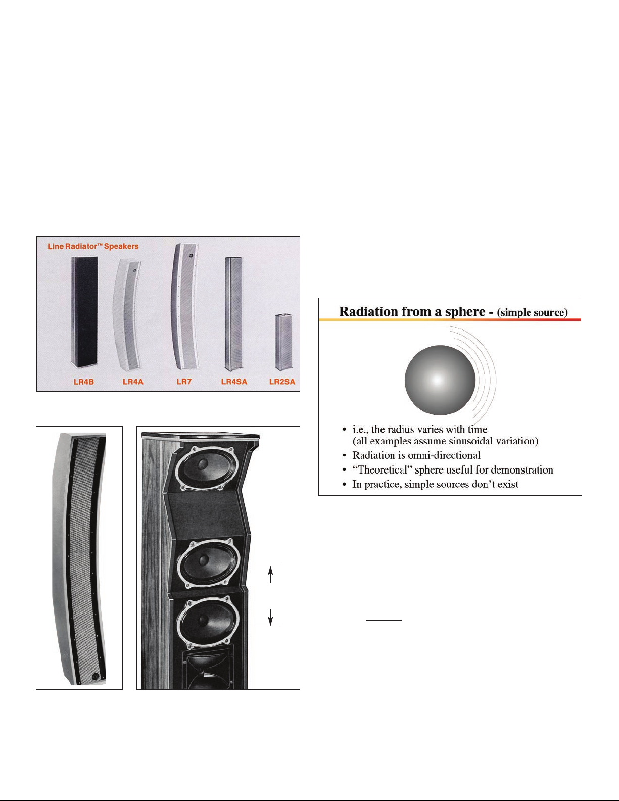
vocal range intelligibility in reverberant spaces. Figure 1,
Figure 2 and Figure 3 are excellent representations of high
performance “vocal range” line arrays. These line arrays, like
all vertically oriented sources in the past were, what could best
be termed, limited bandwidth line arrays.
Figure 3 shows an Electro-Voice line array from the 1970s.
It represents a relatively elegant solution to achieving high vocal
intelligibility. It should be noted that the source separation of
this design is roughly six inches, relating to a wavelength of
2.26kHz. The line array behaved very well up to that 2 kHz range.
It should also be noted in the Figure 3 that a high
frequency horn was employed above that frequency limit in
order to achieve appropriate extended bandwidth and fidelity
up to and beyond 10 kHz. This is a classic embodiment of a
limited bandwidth line array and as we shall see in this presentation, only recently have solutions been brought to the state
of the art to enable line array technology to truly be full bandwidth and extend beyond the 10-15 kHz region.
Before we begin discussing bandwidth for modern day line
arrays, it is important to begin with a discussion of basic
radiation of sound. Figure 4 represents a spherical shape
whose radius “r” can vary with time.
Figure 5, Equation 1 describes the acoustical performance
of this pulsating sphere. This pulsating sphere, or simple
source is a useful theoretical tool describing the mathematics
of radiating sound.
Figure 5, Equation 1
ρ
AV
=
(ka)
2
p.c ( Vs2) ave (4πa2)
1 + (ka)
2
Where: K = W/
C
ρ
AV
= time averaged power
VS= velocity
Figure 5, Equation 2
Condition:Ka << 1
or
λ >> a
Line Arrays
Figure 1
Figure 2
Figure 4
b=6''
ƒ = 2.26 KHz
Figure 3
1
Page 2
One of the key requirements of this pulsating sphere, or
simple source, is that KA is always much less than 1 (Figure 5,
Equation 2). That is to say the wavelength must always be
much greater than the dimensions of the radiating device
itself. An ideal simple source is almost infinitely small and
thereby meets the requirement that KA is always much, much
less than 1.
Simple sources, of course, don’t exist in the real world as
radiating devices always some dimension and those dimensions,
in order to radiate sufficient acoustic power, become large
compared to most audio frequencies. (It is important to define
the term high frequency and low frequency at this point. When
one considers the term high frequency, one always assumes a
particular value associated with that frequency. One could
assume 5 kHz to be a relatively high frequency and it certainly
would be if the radiating device were an 18-inch direct radiating
loudspeaker. 5 kHz conversely, is a very low frequency if the
device radiating that wave front were a very small dimension, a
high frequency super tweeter, for example. The important thing
to note here is that the term high frequency or low frequency
is a term that describes the wavelength in comparison to the
dimensions of the radiating device itself. Throughout this
discussion of line arrays, whenever the term high or low
frequency is used, it is always assumed that a low frequency
has an associated wavelength much longer than the dimensions
of the radiating source and the term high frequency relates to
wavelengths that are much shorter than the dimensions of the
radiating source.)
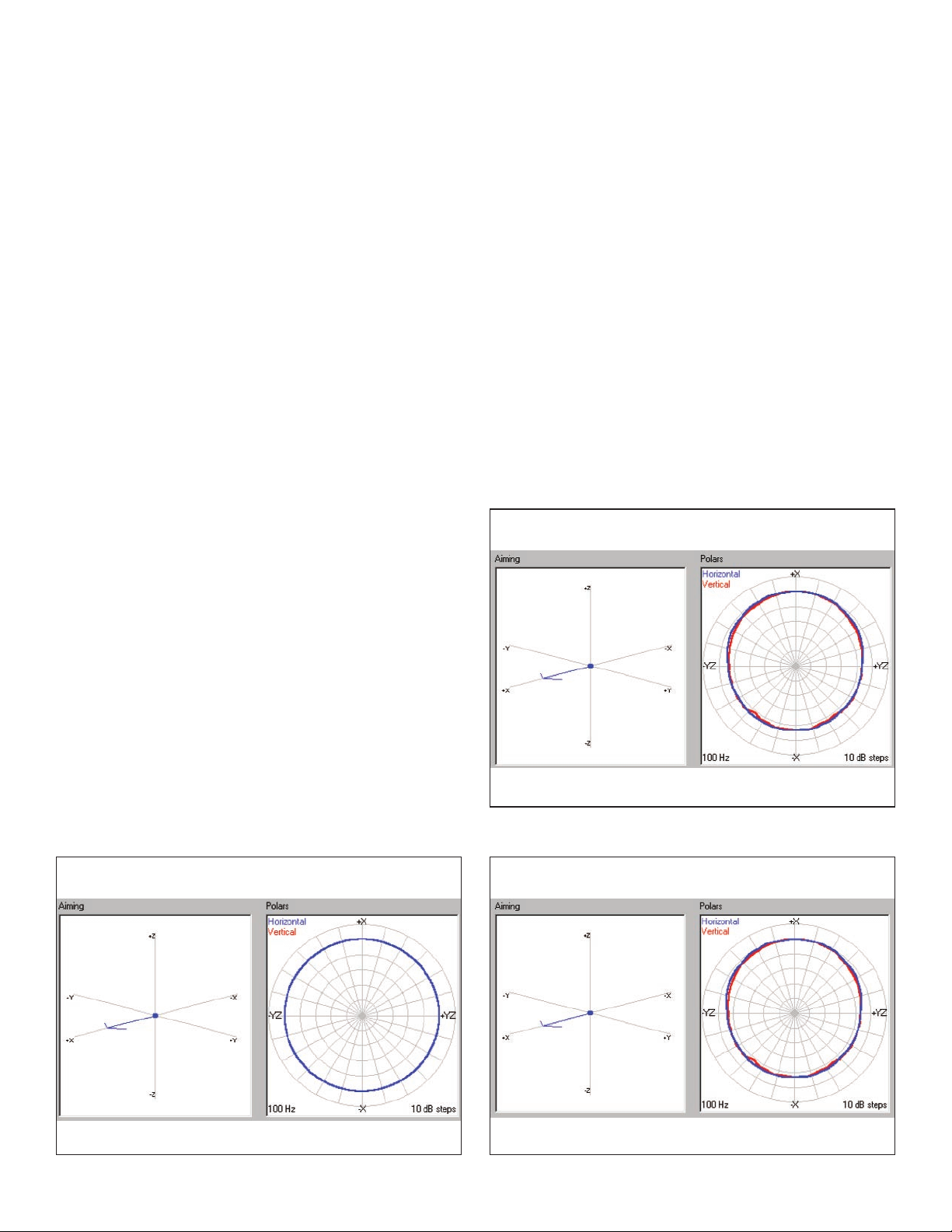
Figure 6 is an Array Show representation of a theoretical
simple source. As can be seen from this slide, the radiation is
purely omnidirectional, implying that any wavelength radiated
is always long compared to the dimensions of the radiating
device. It is common in sound reinforcement practice to
assume that subwoofers or bass enclosures are essentially
omnidirectional.
Figure 7 shows an Electro Voice XDS subwoofer enclosure.
Although the 100 Hz being radiated is a relatively low frequency
(wavelength approximately 11.3 ft), examination of the associated
polar in this figure shows that the radiation at + and – 90
degrees from the central axis is 6dB to 7dB down from that on
axis and the radiation at 180 degrees opposite the main lobe is
also 7dB to 8dB down. The XDS is a relatively large subwoofer
from a physical standpoint. (36''H x 45.92''W x 29.88''D). The
radiator is not omni directional.
To further illustrate the point, Figure 8 shows an Electro
Voice TL15-1 base enclosure. This is a single 15-inch, direct
radiating enclosure of very small dimension. It can still be seen
from examination to polar response in this figure that the
response at +/- 90 degrees is still 3 dB down from that on axis.
Again, not omni directional radiation. These figures, indicate
the importance of the radiated frequencies being substantially
longer than the dimensions of the device if true omni directional radiation is to occur. Given the initial descriptions of
these theoretical simple sources or pulsating spheres it is now
appropriate to bring a second sphere into the discussion.
Figure 6
Figure 7
Figure 8
2
Page 3
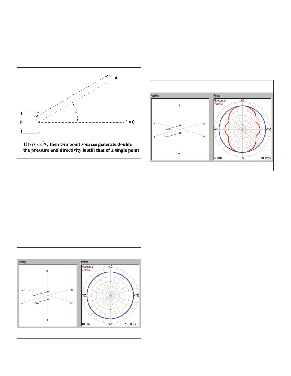
Figure 9 represents two spheres or simple sources separated
by a distance B. The assumption here is that B is always much,
much less than the radiated wavelengths. If this condition
occurs, than the two point sources will generate double the
pressure and the directivity is still that of a single point (omni).
This is a simple and intuitive case where two radiating sources
simply generate twice the pressure of the single source.
Figure 10 shows these two point sources separated by a
distance of 12 inches. The polar response shown is that of
those two point sources radiating 100 hz signal. Again, the
space in B is much, much less than the wavelength, and as a
result, the radiation continues to be that of an omni-directional
condition. (Again, this is only a theoretical case, as point
sources do not exist in practice.) This representation is
extremely useful when we look at Figure 11, which is the same
two point sources as that of Figure 10. The distance continues
to be 12 inches, but now the frequency has been raised to 630
hz. (B approximately equivalent to 1/2 of the wavelength.)
Examination of Figure 11 shows that at 0 degrees on axis
and at 180 degrees the radiation is summing coherently and
the radiation at –90 degrees and +90 degrees (-y/,+y on the
Array Show polar plot) is experiencing cancellation. The
radiation of +x and –x, or that of the radiation on axis, has
seen a 3 dB gain in pressure associated with the pressure
addition of the two sources. Figure 11 begins to illustrate the
principles underlying successful application of a continuous line
of vertical sources (that of a line array).
Figure 12 is extremely interesting as well as it explains
the “historical” applications where line arrays were limited
bandwidth devices, such as those referenced in Figure 1,
Figure 2 and Figure 3 earlier in this discussion. The two point
sources continue to be spaced by 12 inches, but now the
frequency has been raised to 2500 hz. In this case, the space
B is equal to twice the wavelength. Examination of the polar
response shows substantial polar lobing errors. It describes
exactly the response of any group of sources, whether they are
vertically oriented or horizontally oriented when the wavelengths become shorter than the device spacing.
Figure 12 is a clear representation of difficulties that
system designers face when trying to provide full bandwidth
radiation (i.e. greater than 16 kz) with real world radiating
sources. The peaks and nulls in the diagram of Figure 12 are
easily heard in real world applications and have always been
taken as a “necessary evil” when orienting sources. The
previous polar diagrams also require some explanation.
In definition of terms, Figure 13, the beamwidth is
defined as the included angular separation between the –6 dB
points, reference to the 0 db (+x) axis. The term Q is the ratio
of the acoustic intensity on that reference axis at some
reference distance to a true point source radiating the identical
acoustic power. Again, the true point source is useful from a
mathematical standpoint to enable us to define the acoustic
intensity ratio of real world devices to theoretical omni
Figure 9
Figure 10
Figure 11
3
Page 4
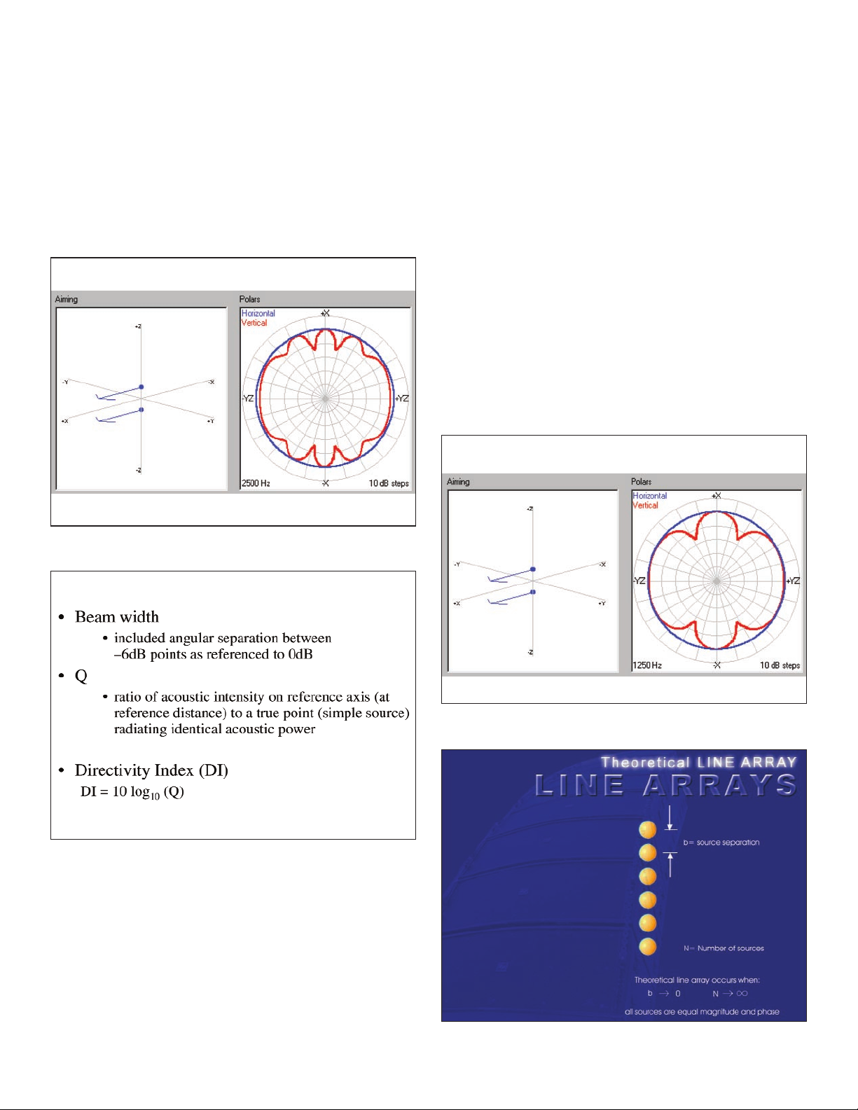
directional radiators. Of most interest when designing line
arrays is the term directivity index. The directivity index,
di = 10 log base 10(Q), represents the acoustic gain associated
with the increased directional radiation of higher Q devices.
The fundamental operation of a vertical source of radiators
or a line array depends heavily on gain related to directivity
index. These gains, of course, are also dependent on having
the directivity index be constant with regards to frequency.
(Constant gain versus frequency is a critical operating parameter
for uniform SPL distribution).
Figure 14 is another Array Show representation illustrating
the concept of beamwidth, Q and directivity index. Here two
point sources, again spaced 12 inches apart, are shown. The
applied frequency is 1250 Hz. In this condition the spacing B
is approximately the equivalent to the wavelength associated
with 1250 hz. In Figure 14 the beamwidth is 30 degrees, the
Q is 2 and the directivity index associated with that Q is
slightly over a 3 dB gain.
It can also be seen from Figure 14 that the lobing pattern
begins to suggest that spacings greater than those equal to
the radiated wavelength begin producing unacceptable polar
lobing errors. For this reason, successful application of full band
with line arrays requires that the spacing always be less than
the radiated wavelengths. Figure 15 now takes our two point
sources and begins to build a continuous vertical orientation of
sources. Although still theoretical in nature, the representation
shown in Figure 15 is exactly what is used to generate the proper
mathematical description of the line array. The sources still have
a separation of B but now we’ve replaced two sources with N
number of sources. A theoretical line array occurs when the
spacing B tends toward 0 and the number of sources grow towards
infinity. Again, although both conditions are impossible to
satisfy in real world applications, the designer’s challenge is to
approximate small source separation and as great a number of
sources as geometry, physical spacing, and safe hanging practice
will allow. It should also be noted that one of the key points
to all line array discussions is noted in Figure 15, and that is
all sources must be both equal in magnitude and of equal phase.
Figure 12
Figure 13
Figure 14
Figure 15
4
Page 5

This last condition is the key to all line array analysis, at
least from a theoretical standpoint. Subsequent discussions of
the line array performance will demonstrate what this condition
of equal magnitude and phase rarely, if ever, occur.. Figure 16
shows a theoretical line array with a large number of vertically
oriented sources. The radiation frequency associated with this
figure is 630 Hz. Examination of the polar pattern shows very
controlled response with very minimal lobing error. Appropriate
examination of this polar for a line array is in the quadrant
from +x to –y (in the Array Show plot). This is the section of
any line array that is used for audience coverage.
Given the definition of the line arrays previous discussed,
we can now begin to look at practical line arrays and their
applications. As noted, we cannot achieve source separation
approaching 0 nor the number of sources approaching infinity.
Practical line arrays or those realizations of line arrays occur
when the space in B is less than the radiated wavelength.
Figure 17 is a key design consideration when designing a full
bandwidth line array system. Practical line arrays not only
require that the radiating elements separation ”B” be less than
the wave lengths radiated for those devices, but subsequent
spacing of cabinets is also required to be very small compared
to the wave-lengths.
In Figure 18, we see a linear arrangement of 8 cabinets.
We have another spacing constant B’ that is required to be very
small. In addition, the line array overall height H must be large
compared to the radiated wavelengths. The device separation B
and line array height H are two key parameters to describe
both the high frequency limits (fmax) and low frequency limits
(fmin) of a line array system. The space B helps to determine
Fmax, the highest frequency of well-behaved summing. The
parameter H defines Fmin, the lowest frequency that the line
array can maintain a constant directivity versus frequency.
As previously noted, the space in B’ (the space between enclosures) must always be less than a wavelength. The array height
H must always be at least 4 to 5 times longer than the longest
frequency of radiation to achieve constant directivity index
versus frequency.
As we will see in subsequent discussions, these two
parameters are the key parameters controlling our overall line
array performance and its bandwidth. As can be seen from
examination of the previous slides, physical orientations of
radiating sources can produce improved directional response.
The improvements in Q and associated directivity index gains
are simply the result of the fact that the radiating sources
(all of the same amplitude and phase) are separated physically
in space and hence the arrival of signals at any given point in
space are at different times and result in either constructive
or destructive addition (peaks and dips in response).
The constructive addition, of course, is the desire of the
system’s designer and understanding the destructive addition
(dips, or cancellation) is necessary in order to fully optimize
the overall system’s results. It has been seen that directional
radiation can be achieved by orientation of simple sources.
Figure 16
Figure 17
Figure 18
5
Page 6

There is, of course, a second way to achieve direction
radiation. That is through directional devices. The most universal
directional device is a horn. Figure 19 shows a single horn
with radiating device (a compression driver) mounted to the back
section of the horn. This small entrance, or throat, is coupled
to the air via the length of the horn and the horn mouth.
Figure 20 shows three horns oriented in a vertical fashion.
In this case, the minimum spacing achievable because of the
dimensions of the horn themselves is 9.25 inches.
Figure 21 is a polar presentation of the radiation from those
3 vertically oriented high-frequency horns at 5,000 hz. This
frequency was chosen because it is small compared to the
device spacing and the associated vertical polar pattern shown
in this figure should be familiar to anyone who’s ever tried to
make vertical stacks of high frequency horns in an attempt to
improve the directional radiation. Although the radiation is
certainly improved (the Q is increased and as a consequence
there is more gain on the major axis), examination of the figure
shows substantial polar lobing error (i.e. nulls of up to 15 dB
from the on axis reference). This vertical orientation of devices,
although producing an improved directivity index, would suffer
from substantial lobing errors as one walks from the +x axis
to the –y (that is, walk from the front of the array toward the
back of a venue covering the entire included vertical angle of
the venue).
Figure 22 shows an Array Show plot of a point source
and compares it to the Array Show plot of the directional
improvements in response associated with the application of
the horn. It can be seen that the directivity of the devices
is indeed improved, but as noted in the previous figure, an
attempt to generate a continuous line source of the devices
is limited by the physical dictates of the device dimensions.
Again, in this case, a 9.25 inch spacing is as close as they
can be physically positioned which limits Fmax for the highest
frequency of acceptable summing to below 2 kHz. Nevertheless,
horns are very useful devices and basically perform two
functions.
The first function is that of “directing” wave fronts that
are comparable to or shorter than the horn dimensions in a
given area. This is achieved simply by virtue of the sides and
top and bottom walls of the horn. Again, it should be reinforced,
the horn is only capable of this control of radiation where the
wavelengths are comparable or shorter than the dimensions of
the horn itself, (that is, for high frequencies, as defined earlier
in this paper.)
Figure 19
Figure 20
Figure 21
Figure 22
6
Page 7

The second function of the horn is that of an acoustic
transformer. Figure 23, Equation 3, represents how the acoustic
transformer is physically realized in a horn. The diaphragm
radiating the energy has an area vdand an area ad. That radiated
energy is transmitted into the small section, or throat, of the
horn. The velocity of air in that throat is represented by vtand
the area of the throat is represented by at. Conservation principles
require that:
VDAD= VTA
T
Let VD= 4 in/sec
AD= 4 in 2
AT= 1 in 2
VDAD= VTA
T
(4) (4) = VT(1)
VT= 16 in/sec
Where VD= velocity of diaphragm
AD= area of diaphragm
VT= velocity in throat
AT= area of throat
A simple example is shown in Figure 23, Equation 3 where
we arbitrarily set vdto 4 inches per second and the area of the
diaphragm is arbitrarily set to 4 square inches (these are
thoroughly arbitrarily quantities simply selected to make the
arithmetic very simple). We now arbitrarily set the area of the
throat to 1. This is where the term compression driver comes
from, as the area of the radiating diaphragm is many times
greater than the area of the throat. The air displaced by the
diaphragm then encounters a substantially reduced area in the
throat. The air is compressed and the diaphragm is able to “do
more work” against the air in the throat. In the example here
using the arbitrary parameters, the equation becomes as shown.
Solving for vtgenerates 16 inches per second, a substantial
gain over the physical velocity of the diaphragm itself. In this
case we have the velocity in the throat substantially greater
then the velocity of the diaphragm, and we generate an additional conversion efficiency as a result.
We have now illustrated two methods of achieving
directional radiation, that of orientation of simple sources or
of coupling a horn to a radiating source. An important concept
at this point is to introduce the product theorem.
ρ
(r, ~ ,ø) =
ρ
AX
(r) | He ( ~ ,ø) H ( ~ ,ø) |
Where He ( ~ ,ø) is the expression
that describes the
directional characteristics
of each source.
The product theorem is shown in Figure 24, Equation 4.
The explanation of this equation is very simple and again, is
a key to our physical realization of an effective line array. The
product theorem simply says that a simple source array has a
multiplying factor that is described by the directional nature
or “Q” of each horn loaded element. Or put another way, the
result of a nonsimple array equals the simple array directionality
plus the individual device directionality.
Figures 25 and 26 illustrate this very graphically. Figure 26
should be familiar. It, again, is the a long vertical arrangement
of simple point sources each spaced 12 inches apart. The
frequency is 630 Hz and, again, is relatively long compared to
the device spacing (in this case, the wavelength is 2 times the
device spacing). Comparison of this polar with the same array
where the simple sources have been replaced with horns, each
bringing their own directionality, shows the change in vertical
radiation. Substantially higher Q and associated higher directivity
index are the result of the combination of the directionality of
the array with the simple sources and a multiplier of that
directivity that is the directionality of each horn device that
has replaced the simple radiating source.
Figure 24, Equation 4
Figure 25
Figure 26
Figure 23, Equation 3
7
Page 8

Realizing a Full Bandwith Line Array
Full bandwidth line arrays are typically three way systems.
The practice of dividing the band into 3 separate passes is
done to enable the cross-over points to always be substantially
low enough that the radiation from each pass exhibits wavelengths that are always longer than the physical device, or driver
spacing. This is relatively easy to achieve for the low frequency
section of any line array and is also easy to achieve for the
mid-band section.
In mid-band sections the mid range devices are 6 inches
in diameter to 8 inches in diameter. The crossover points are
selected so that the device spacing is always small compared
to the wavelength radiated. The problem for a full bandwidth
line array systems is the high frequency radiation.
As mentioned earlier, historical line arrays were excellent
in terms of low frequency and mid-band control of the pattern,
but always suffered from polar lobing errors associated with
the device space “B” being greater than the wavelengths being
radiated. A 16 kHz wavelength is on the order of 3/4 of an
inch and as a consequence device spacing must be comparable
to those wavelengths or shorter, if possible. This was always
a problem in the past because engineering techniques could
not realize spacing closer than the driver diameters themselves.
Even with modern neodymium iron boron based magnetics,
the diameters were always at least 4 inches or greater (for
large format diaphragm devices). That spacing limited good
performance to below approximately 3 kHz, obviously not a full
bandwidth device.
As a practical example, fmax, the maximum high frequency
control based on the relationship between the spacing of the
devices b and the wavelengths is as follows. For base line
arrays where we are interested in control up to 250 hz, the
spacing needs to be at least 4.5 feet. This is relatively easy
to do with 15 inch and 12 inch drivers and as a result the realization of bass frequency line arrays is very straightforward.
For mid-band line arrays, if we are interested in frequencies
between 250 and 1,250 hz, the spacing needs to be 11 inches
or smaller. Again, this is relatively easy to do with 6 inch or
8-inch drivers, and this is frequently the diameter of mid range
devices in both large format and compact line array systems.
Figure 27 shows an Electro Voice Hydra™. This device
basically takes the radiation of a compression driver and acts
to produce both equal amplitude and equal phase sources at
the front of the wave-guide. The full drawing in Figure 27 is 3
Hydras vertically stacked, thereby generating 21 “point source”
radiating surfaces coupled to a horizontal wave guide with an
included angle varying between 90 and 120 (model dependent).
Figure 28 shows a Hydra without the driver or wave-guide
coupled. Each hydra has 7 output “slots”. The driver is coupled
to the input side of the hydra and the 7 outputs are then
interfaced with a horizontal wave-guide to produce the
required horizontal included angle. The space b for a hydra is
.826 inches, which equates to a wavelength of 16,434 Hz.
Again, it is always best for wavelengths to be longer than that
spacing, so in this implementation, the Hydra presents excellent high frequency control in the 15kHz to 16 kHz range. The
Array Show plot Figure 29 shows 21-point sources in a vertical
orientation with the exact spacing provided by a hydra.
Figure 27
Figure 28
Figure 29
λ = 16,434 Hz
8
Page 9

Realized Line Arrays/Horizontal Geometry
Figure 30 represents two possible methods of orienting a
full bandwith line array. The two methods are axis symmetric
and axis asymmetric. The most common realization is that of
an axis symmetric. It is the left hand drawing on Figure 30.
The high frequency section is in the horizontal center of the
enclosure and is flanked by two mid drivers of 6 to 8 inch
diameter and two low frequency drivers of 12 inch to 15-inch
diameter (depending on individual realization).
One of the advantages of an axis symmetric design is that
horizontal response is the same either side of the center axis.
Figure 31 slows a close up of an axis symmetric design. Of
course one of the consequences for axis symmetry is that
devices now become horizontal “arrays”. For most of this paper
we’ve focused our discussions on vertical orientation of arrays,
but it should be remembered that the same directional
response characteristics exist for devices whether they are
oriented vertically or horizontally.
There is a common mistake in sound reinforcement practice for people who normally understand that stacking devices
vertically will control the vertical pattern to then stack devices
horizontally in the misguided attempt to increase the horizontal
radiation pattern. This is something termed array arithmetic.
In normal arithmetic, 40 + 40 + 40 will always equal 120. This,
unfortunately, is not always the case with acoustics. In the
same example, three enclosures stacked horizontally are usually
done so because the array designer or the person developing
the array has a desire to cover an included angle of 120
degrees (an example). The three 40 degree devices stacked
horizontally will add to 120 degrees under certain conditions.
They will also add to 20 degrees when the wavelengths are
comparable to the spacing between the devices. This, again,
takes us back to the exact discussions we’ve seen earlier in
this paper with regards to vertical stacking. It should be
remembered by all designers that stacking, whether the arrays
are horizontal or vertical, will always narrow the pattern in
the axis that the devices are oriented. This brings us back to
the mid range devices and low frequency devices in an axis
symmetric design. These axis symmetric designs are small
horizontal arrays.
Figure 32 shows two eight inch drivers separated by a
one-inch exit vertical slot for high frequency radiation. The
two mid devices are oriented into a 90 degree included angle,
but this spacing results in a horizontal array that exhibits the
polar performance illustrated in Figure 33. When a cross over
frequency of 1250 Hz is used, the response is basically 6 dB
down at 30 degrees off axis generating an included angle of
60 degrees, not the 90 degrees desired by the designer of the
product. This is the result of the classic “horizontal array” and
will always occur when the crossover point is comparable to
the device spacing. This, of course, can be eliminated by taking
the crossover frequency substantially lower. Unfortunately,
compression driver performance, in terms of mechanically
generated distortion products and device reliability are severely
compromised in the 700 to 800 region that is required for this
type of device spacing. This is a classic trade-off seen often in
acoustics where one parameter is optimized at the expense of
a second parameter.
In this case, to achieve proper horizontal radiation and
the desired included angle, the distortion, fidelity and
reliability of the compression drivers are compromised; in order
to produce proper fidelity, polar response is compromised.
An alternate approach is the axis asymmetric design also
shown in Figure 30. In this design, there are no horizontal
arrays. The trade-off, of course, is that the device voicing is
not the same on the left hand side of the system as the right
hand side. This, however, can be seen as a minor trade-off
because the horizontal pattern is substantially improved and as
a result, stereo imaging is enhanced. It has often been argued
Figure 30
Figure 31
9
Page 10

that the asymmetrical voicing produced by the axis asymmetric
design is a design compromise but it can be seen as less of a
compromise than that of the axis symmetric where the pattern
begins to narrow or the sonic performance of the drivers is
compromised because of using too low of a crossover frequency.
The second important parameter in line array design is
that of the minimum control frequency. We’ve discussed fmax,
the high frequency control that is limited largely by the spacing b between devices. Discussion of fmin is also appropriate.
The low frequency control of the line array is dictated by the
physical height h of the array itself in Figure 34, Equation 5.
This is very analogous to the low frequency control of the
conventional horn related to its mouth height. Figure 34,
Equation 5 shows that fmin equals a constant over the product
of the required included angle and the height. As can be seen, f
min with a horn is related or is proportional to its overall
height. This is exactly the case for fmin with a vertical orientation of sources, or a line array.
ƒmin =
K
(included angle) (h)
Figure 35 shows the low frequency performance of a line
array related to its overall height. It shows both a multiple of
4 and a multiple of 5. This could be easily misconstrued that
the number of boxes controls the low frequency cut-off. This
is only indirectly the case. The actual parameter is the physical
height of the array, so large format, concert level line arrays
like the EV X-Line certainly require less boxes to get to a
particular cut-off frequency. The important thing to note from
Figure 35 is that if we average the 4 multiplier and 5 multiplier,
we see that a four box system in the case of a compact line
array (the XLC from Electro Voice) is limited to a 1,000 hz
control frequency, which relates to an overall line height of 58
inches. Frequently line arrays are presented that are 20 or 30
inches tall. These are certainly line arrays from a high frequency
standpoint, if the criteria is achieved to produce a full bandwidth f max. Their ability to control the polar pattern at low
frequencies, however, is limited by their height. To achieve a
300 hz low frequency intercept, or fmin, the overall height
of the line array system needs to be roughly 203 inches.
Figure 35 is very instructive in terms of designing line arrays
to low frequency control limits.
An alternate way of looking at this chart and looking at
this parameter is seen in Figure 36. This shows the beamwidth
versus the frequency for a 58-inch high line array and a 116
high line array, doubling the height, as one would expect,
reduces, or improves the control by one octave. It is also
interesting to note that if one desires a 150 Hz line array
control, the line array must be 406 inches tall (almost 34 feet
tall), which certainly is taller than typical line array systems.
Figure 32
Figure 33
Figure 34, Equation 5
Figure 35
10
Page 11

It illustrates the same point that people are used to seeing
with basic horns, that is, the lower the frequency of control,
the larger the mouth must be.
Line Array Performance and General Geometry
The vertical profile of a line array can either be symmetrical
or asymmetrical. What is meant by that is that you can either
have a straight-line array or a curved section but symmetry
still exists about the center axis of the system. The sharpest
beam width will occur for flat or linear line arrays. The higher
the number of sources (n) the more the polar lobing errors are
minimized. This condition occurs independent of the physical
realization or design of the line array itself, and is purely related
to the number of radiating surfaces. Symmetrical curved arrays
broaden the beam width as compared to flat arrays. The more
the curve (the less the radius), the broader the beamwidth. The
third type of profile is that of an asymmetric design. This is
typically the case where there is a curved or flat section on
the top of the array and a more curved or (j) section at the
bottom. The result of this j is to further increase the included
vertical angle of the system, but also to tilt the major lobe.
This tilt is accomplished via the steering properties of the
asymmetrical portion of the array.
Figure 37 shows the vertical lobe generated from a
perfectly flat (or standard linear) line array. It can be shown
that the lobe is extremely sharp and it should always be
remembered that the major lobe emanates from the vertical
center of the system. Early applications of line arrays consisted
of aiming the systems with a laser mounted on the top of the
overall array. This is very inappropriate as can be seen from
any of the figures (Figure 37, Figure 38 and Figure 39).
Regardless of the shape, whether flat, symmetrical, curved
symmetrical, or asymmetrical, the major lobe always emanates
from the physical center of the system and may be steered by
the asymmetrical portion of the array, but generally continues
to emanate from the center. Figure 38 shows a curved array,
and again, shows symmetry about the center axis of the array.
Figure 39 is a classic J array, and examination will reveal a
lobe very similar to that of Figure 38 with the addition of the
increase in energy toward the bottom half of the array, where
the j curve is steering the system. Figure 40 is an idealized
representation of a flat or linear source, showing the center of
the acoustic lobe emanating from the vertical center of the
system. It also represents “old custom” of a laser mounted at
the top and assuming the top box pointed at the back of the
venue presented a major potion of the energy into that area.
As can be seen very quickly from the simple example the
response with a proper line array is very high Q and the amplitude falls off very rapidly from either side of the center of the
acoustic cube. This is desirable working below the center of the
acoustic lobe, as proper aiming can, in fact, compensate for
attenuation of sound with distance and produce remarkably
even front to back coverage. That advantage becomes a
disadvantage if the upper portion of the lobe is attempted to
be used to cover the audience in the rear portion of the venue.
Figure 36
Figure 37
Figure 38
Figure 39
11
Page 12

Line Arrays and Very Low Frequencies
Traditional practice with low frequency radiators, or
subwoofers, has been to groundstack the subs. Groundstacking
produces the familiar 3 db doubling of pressure, because of
the conversion in the acoustic load from a 4π steradian to 2π
steradian load. Figure 41, Equation 6 and Figure 42,
Equation 7 show the change from full space to half space
loading and the subsequent pressure doubling. The physical
height requirements of a full band with line array, however,
bring an important performance advantage to flying subs. While
it is completely true that the pressure doubling is lost when
the subs are removed from the floor, there is a substantial gain
associated with a large vertical array of low frequency sources.
Full space pressure
ρ
~
p.c
QK
4πr
Half space pressure
ρ
1
/2 ~ p.c
QK
2πr
Figure 43 shows polar response of a 3 by 3 groundstack.
The vertical control gained via not only the geometry of the
stack itself, but because of the coherent reflection of the floor.
A 12 high flown array is shown in Figure 44. Although the
polar pattern is partly compromised, the Q is substantially
increased. The associated gain in directivity index is a very
valuable tool for a system designer. In Figure 45 shows a
typical groundstack. A 200-foot long room would exhibit the
following performance. A flow line array would generate, if
properly aimed, a +/– 1dB to 2 dB variation front to back
in the venue described in the example. In that same situation,
the groundstacked sub would exhibit a 24-1/2 db variation of
low frequency material from the front to the back. This is an
obvious compromise in the full bandwidth control (or directivity
index versus frequency control) of the system. With proper
aiming, a 12 box high vertical line array of low frequency
material can substantially improve the overall front to back SPL
coverage of very low frequencies. Although this 12 box hang
is nowhere near high enough to control 100 Hz and below, the
improvement in uniformity of front to back is 5 to 10 times
better than that of the groundstack. Because of that improvement in front to back uniformity, flying subs are highly recommended where improved full frequency coverage is required.
Figure 40
Figure 42, Equation 7
Figure 41, Equation 6
Figure 45
Figure 43
Figure 44
12
Page 13

SUMMARY
Many claims have been made in recent years as to the
“unique” performance characteristics of modern line array
systems. The simple reality is that, for standard, curved or “j”
arrays the performance is very well behaved because the device
spacing and cabinet spacing are always small or comparable to
the wavelengths being radiated. It is simple and straight forward.
The attenuation of SPL is 6dB per every doubling of distance
from the system (in the far field). That is exactly the behavior
of a classical spherical radiating source. It is true that linear
sources can exhibit a reduction of only 3dB for each doubling
of distance but this occurs only in a limited section of the
near to far field transition and is frequency dependent. What is
more noteworthy is that this 3dB per doubling of distance
behavior is only possible when the array geometry is perfectly
flat. Initial line array users attempted to use flat arrays and
always noted unacceptable included vertical angle performance
(whether indoors or outdoors) and also noted extreme difficulty
in matching the SPL coverage versus distance in the venue
with the flat array’s major lobe (for curved arrays the near field
behavior is likely between 3dB and 6dB per doubling of distance
and is very difficult to quantify).
It should also be noted that line arrays, although offering
substantial benefits, are not suited for all applications. A line
array needs proper aiming or sub standard performance will
result. Line arrays are not suited for low ceiling venues or
venues that don’t generally match the included horizontal
angle of the system. Conventional “cell arrays” of high Q
elements, although suffering from all of the polar lobing errors
noted in this paper, are often a better overall solution for low
ceiling environments or long and narrow rooms.
Any attempts to use line arrays without good “application
specific” aiming software can result in more frustration than
success. Many manufacturers offer good line array CAD routines
that will enable an educated user to achieve excellent results.
An additional advantage of aiming software is that it can
be an excellent educational tool. A novice user can quickly
work through a large variety of line array geometry and venue
styles and easily see all of the concepts discussed in the paper
come into practice.
13
 Loading...