Dwyer Instruments UFB-222, UFB-122, UFB-223, UFB-123 User manual

Download

Series UFB Ultrasonic Flowmeter Kit

Installation and Operating Instructions

Bulletin F-UFB

Find Quality Products Online at: sales@GlobalTestSupply.com

www.GlobalTestSupply.com

Table of Contents

1: General Description 1

1.1 Introduction 1

1.2 Principles of Operation 2

1.3 Supplied Hardware 3

1.4 UFB Instrument 4

1.4.1 Connections 4

1.4.2 Keypad 4

1.4.3 Power supply 5

2: Installation 6

2.1 Safety Precautions and Warnings 6

2.2 Installing the UFB Instrument 6

2.2.1 Positioning the instrument 6

2.2.2 Mounting the instrument 7

2.2.3 Connecting the instrument 8

2.3 Installing the Ultrasonic Transducers 9

2.3.1 Transducer positioning 9

2.3.2 Transducer attachment 10

2.3.3 Attaching the guide rail to the pipe 11

2.3.4 Fitting the transducers 11

2.3.5 Transducer attachment (diagonal mode) 14

3: Operating Procedures 16

3.1 Setting-up the Instrument 17

3.1.1 Using the instrument for the first time 17

3.1.2 Changing the user language 17

3.2 Using the Quick Start Menu 18

3.3 Instrument Calibration 22

3.3.1 Adjusting the zero cut-off 22

3.3.2 Adjusting the set zero flow offset 22

3.3.3 Adjusting the calibration factor 23

3.3.4 Adjusting the roughness factor 24

3.3.5 Adjusting the damping factor 24

3.4 Outputs 26

3.4.1 Current output 26

3.4.2 Pulse output 28

3.4.3 Alarm outputs 29

Find Quality Products Online at: sales@GlobalTestSupply.com

www.GlobalTestSupply.com

Table of Contents (Cont.)

3.5 How to Measure Totalized Flows (manually) 32

3.6 Display of totalizers 33

3.7 Setting the Chiller Options 33

3.7.1 Setting the Chiller Delay 34

3.8 Operation with an Energy Meter 35

3.8.1 Pulse output 35

3.8.2 Configuring the UFB 35

4: Maintenance & Repair 37

4.1 Introduction 37

4.2 General care 37

4.3 Warranty / Return 37

5: Troubleshooting 38

5.1 Overview 38

5.2 General Troubleshooting Procedure 39

5.3 Warning and Status Messages 40

5.4 Diagnostics Display 42

6: Options 43

6.1 Large Pipe Diameter Transducers 43

6.2 Transducer Holder Options 43

6.3 Extended Signal Cable Options 43

7: Specification 44

Find Quality Products Online at: sales@GlobalTestSupply.com

www.GlobalTestSupply.com

1: General Description

1.1 Introduction

This manual describes the operation of the UFB flowmeter. The flowmeter is designed to work with clamp-on transducers to enable the flow of a liquid within a closed pipe to be measured accurately without needing to insert any mechanical parts through the pipe wall or protrude into the flow system.

Using ultrasonic transit time techniques, the UFB is controlled by a micro-processor system which contains a

wide range of data that enables it to be used with pipes having an outside diameter ranging from 0.5 to 79 inches (13 to 2000 mm) and constructed of almost any material. This can be extended to pipes of up to 197 inches (5000 mm) using the optional type D sensors. The instrument will also operate over a wide range of fluid temperatures.

UFB standard features:

• Large, easy to read graphic display with backlight.

• Simple to follow, dual function keypad.

• Simple ‘Quick Start’ set up procedure.

• Continuous signal monitoring.

• Isolated pulse output (volumetric or frequency).

• Isolated current output (4 to 20 mA, 0 to 20 mA, or 0 to 16 mA).

• 2x Isolated programmable alarm outputs.

• Password-protected menu operation for secure use.

• Signal diagnostics.

• Multi-function alarm outputs.

• Operates from Mains, 24 Vac, or 24 Vdc.

Volumetric flow rates are displayed in L/h, L/min, L/sec, gal/min, gal/h, USgals/min, USgals/h, Barrel/h, Barrel/ day, m³/s, m³/min, m³/h. Linear velocity is displayed in meters or feet per second. When operating in the ‘Flow Reading’ mode the total volumes, both positive and negative, are displayed up to a maximum 12-digit number.

The flowmeter can be used to measure clean liquids or oils that have less than 3% by volume of particulate content. Cloudy liquids such as river water and effluent can be measured along with cleaner liquids such as demineralized water. Typical UFB applications include:

• Sea or River water.

• Potable water.

• Demineralized water.

• Treated water.

The UFB is available in two model options. Model UFB-A is supplied with type ‘A’ transducers which are designed to work with pipe diameters between 0.5 to 4.5 inches (13 to 115 mm). Model UFB-B is supplied with type ‘B’ transducers which are designed to work with pipe diameters between 2 to 79 inches (50 to 2000 mm). Both sets of transducers use a common mounting system for pipe attachment, and throughout this manual any reference to ‘UFB’ applies to both ‘A’ and ‘B’ model variants unless otherwi

se stated.

Note: In addition to the 'A' and 'B' type sensors, type 'D' sensors (option) are available for use on pipes up to 197 inches (5000 mm). These sensors have a different mounting method. See Paragraph 1.3 for further details.

Find Quality Products Online at: sales@GlobalTestSupply.com

www.GlobalTestSupply.com

1: General Description

Fluid flow

Separation

Distance

Separation

Distance

Separation

Distance

Separation

Distance

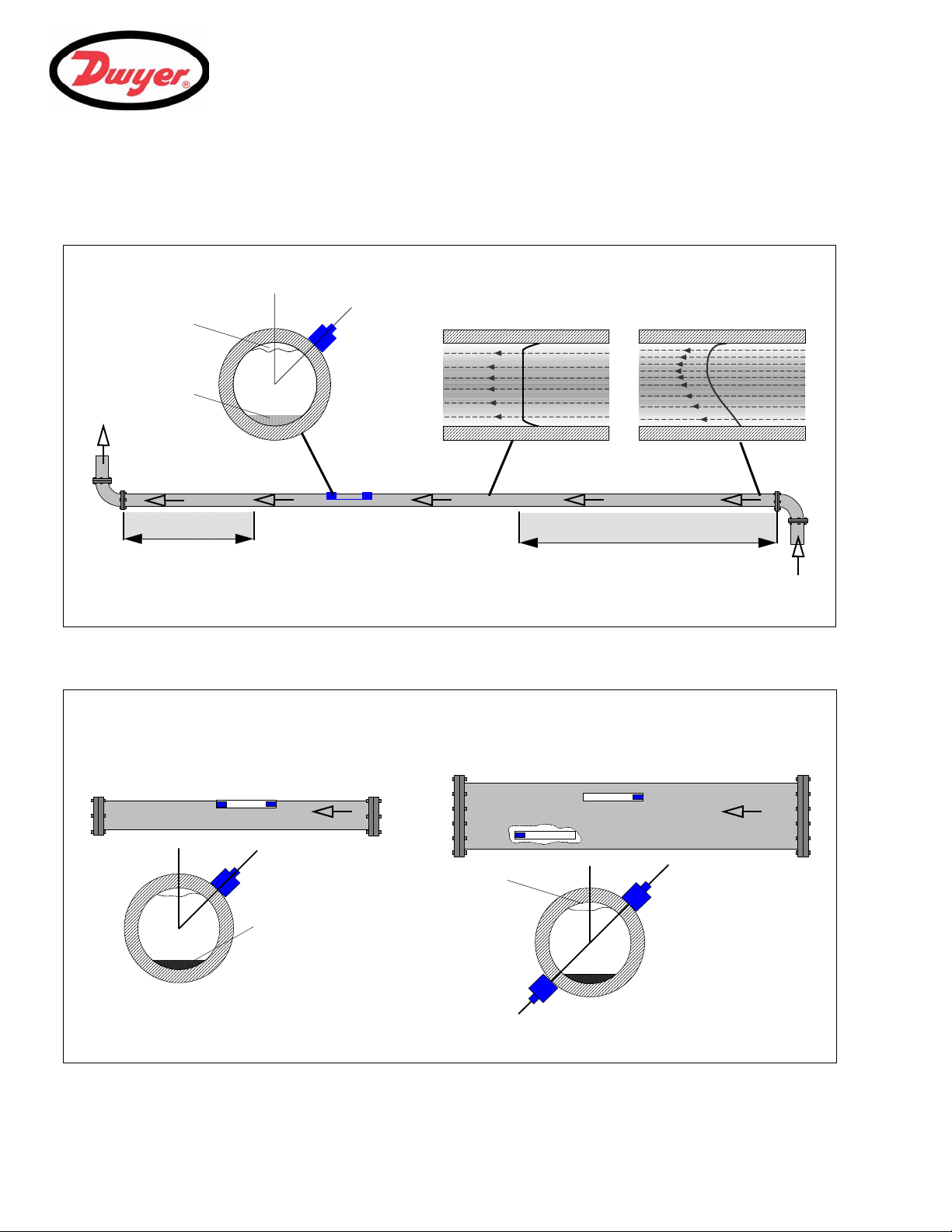
Reflex mode

Reflex mode (double bounce)

Reflex mode (triple bounce)

Diagonal mode

This is the mode most commonly used. The two transducers (U & D) are attached to the pipe in line with each other and the signals passing between them are reflected by the opposite pipe wall. The separation distance is calculated by the instrument in response to entered data concerning the pipe and fluid characteristics.

In this mode the separation distance is calculated to give a double bounce. This is most likely to occur if the pipe diameter is so small that the calculated reflex mode separation distance would be impractical for the transducers in use.

This illustration goes one step further to show a triple bounce situation. This would normally apply when working with very small pipes relative to the transducer range in use.

This mode might be selected by the instrument where relatively large pipes are concerned. In this mode the transducers are located on opposite sides of the pipe but the separation distance is still critical in order for the signals to be received correctly.

This mode can be used with the standard ‘A’ & ‘B’ transducer sets but for really large pipe installations the optional transducer set ‘D’ might be recommended.

Upstream

transducer

1.2 Principles of Operation

When ultrasound is transmitted through a liquid, the speed at which the sound travels through the liquid is accelerated slightly if it is transmitted in the same direction as the liquid flow, and decelerated slightly if transmitted against it. The difference in time taken by the sound to travel the same distance but in opposite directions is therefore directly proportional to the flow velocity of the liquid.

The UFB system employs two ultrasonic transducers attached to the pipe carrying the liquid and compares the time taken to transmit an ultrasound signal in each direction. If the sound characteristics of the fluid are known, the instrument’s microprocessor can use the results of the transit time calculations to compute the fluid flow velocity. Once the flow velocity is known the volumetric flow can be easily calculated for a given pipe diameter.

Figure 1.1 Operating modes

Find Quality Products Online at: sales@GlobalTestSupply.com

www.GlobalTestSupply.com

The system can be set up to operate in one of four modes, determined mainly by the pipe diameter and the type

Acoustic

Steel

Transducer

Transducers (Sensors)

UFB Instrument

Mounting

Earthing

Transducer Cables (x2)

User Documentation

Holder

Couplant Applicator

(Ax2, or Bx2)*

Clamps (x2)

Bands (x2)

Cable Kit

Transducer Clamps

of transducer set in use. The diagram in Figure 1.1 illustrates the importance of applying the correct separation distance between the transducers to obtain the strongest, and therefore most reliable, signal.

1.3 Supplied Hardware

The supplied UFB components are shown in Figure 1.2.

1: General Description

Figure 1.2 Standard UFB equipment

UFB Standard equipment

Find Quality Products Online at: sales@GlobalTestSupply.com

UFB Optional equipment

• Instrument with backlit graphic display.

• Transducer cables (x2) 16.5 feet (5.0m) in length.

• Transducers ‘A-ST’ x2 (UFB-A) for use with pipes ranging 0.5 to 4.5

• Transducers ‘B-ST’ x2 (UFB-B) for use with pipes ranging 2 to 79 Inches (50 to 2000 mm).

• Transducer holder for use with ‘A’ or ‘B’ transducers.

• Steel bands used to secure the transducer holder to the pipe.

• Acoustic couplant.

• User documentation.

• Transducer set 'D' can be used for monitoring pipes of 59 inches to 197 inches (1500 to 5000 mm) outside

diameter, over a temperature range -4°F to +176°F (-20°C to +80°C). This optional kit is supplied in a separate case and includes the type 'D' transducers together with ratchet straps and holders for attaching the transducers to the pipe.

inches (13 to 115 mm).

www.GlobalTestSupply.com

1: General Description

Keypad

LCD Display

Coaxial cables to transducers

Cable glands for

Small & Large Glands for power connection

Alarms & I/O connections

Blue = Downstream Red = Upstream

1.4 UFB Instrument

The UFB is a microprocessor controlled instrument operated through a menu system using an inbuilt LCD display and keypad. It can be used to display the instantaneous fluid flow rate or velocity, together with totalized volumes. The instrument also provides an isolated current output, or variable pulse output, that is proportional to the measured flow rate and can be scaled to suit a particular flow range. Two isolated alarm outputs are provided which can be configured in a number of ways. For example, to operate when the flow rate exceeds a specified maximum or minimum value.

1.4.1 Connections

Transducer connections

The transducers are connected to two coaxial sockets located on the bottom left-hand of the instrument. The silkscreen above these connectors show a red and blue triangle and a direction of flow symbol. For a positive flow reading, it is important that the upstream transducer is connected to the RED socket and the downstream transducer to the BLUE one. It is safe to connect or disconnect these cables while the instrument is switched on.

4 to 20 mA, ‘Pulse’, and Alarm I/O connections

The 4 to 20 mA, ‘pulse’, and alarm I/O cables, enter the bottom of the instrument via two cable glands and connected internally to a terminal block. Full details of the terminal connections are provided in Chapter 2 (Installation).

Power supply

Two cable glands located on the bottom right-hand side of the instrument are available for the power supply cable. Two sizes of glands are provided to accept cables of different diameters.

1.4.2 Keypad

The instrument is configured and controlled via a 15-key tactile membrane keypad, as shown in Figure 1.4.

Figure 1.3 Instrument details

Find Quality Products Online at: sales@GlobalTestSupply.com

www.GlobalTestSupply.com

1: General Description

Scroll UP

ENTER (SELECT)

Scroll DOWN

Scroll LEFT

Scroll RIGHT

Numerical keypad with dual function keys

Figure 1.4 UFB Keypad

Menus and the menu selection keys

Note: As a security measure, once the instrument has been set-up for the first time, a password is required to

gain subsequent access to the operating menus (see page 20).

The UFB menus are arranged hierarchally with the MAIN MENU being at the top level. Menu navigation is achieved by three keys located on the right hand side of the keypad which are used to scroll UP and DOWN a menu list and SELECT a menu item. When scrolling through a menu, an arrow-shaped cursor moves up and down the left hand side of the screen to indicate the active menu choice which can then be selected by pressing the ENTER (SELECT) key.

Some menus have more options than can be shown on the screen at the same time, in which case the overflowed choices can be brought into view by continuing to scroll DOWN past the bottom visible item. Menus generally ‘loop around’ if you scroll beyond the first or last items.

If you select Exit on any menu it usually takes you back one level in the menu hierarchy, but in some cases it may go directly to the ‘Flow Reading’ screen.

Some screens require you to move the cursor left and right along the display as well as up and down. This is achieved using keys 5 (scroll LEFT) and 6 (scroll RIGHT).

Dual function numerical keypad

The block of keys shown in the center of the keypad in Figure 1.4 are dual function keys. They can be used to enter straight-forward numerical data, select the displayed flow units, or provide quick access to frequently required control menus.

1.4.3 Power supply

Mains supply

As standard, the UFB instrument is designed to work with a mains supply of 86 to 236 Vac and 50/60 Hz. A mains supply fuse is located adjacent to the mains power connection (see Figure 2.2).

24V Supply

An alternative 24 V (ac/dc) power supply module is available as a factory fitted option.

Power failure

The instrument will automatically power-up and become operational when the input power is applied. In the event of a power failure, the instrument’s configuration parameters are stored in non-volatile memory which then allows the instrument to return to normal operation immediately power is restored.

Find Quality Products Online at: sales@GlobalTestSupply.com

www.GlobalTestSupply.com

2: Installation

WARNING

Caution

2: Installation

2.1 Safety Precautions and Warnings

You may be exposed to potentially lethal (mains) voltages

when the terminal cover of this instrument is removed.

Always isolate the supply to this instrument before removing

This instrument must be installed by an electrically qualified

technician aware of the potential shock hazards presented

when working with mains powered equipment.

LETHAL VOLTAGES

the terminal cover.

LETHAL VOLTAGES

If the equipment is powered from a 24 Vac supply then the

Blanking plugs are fitted to the cable glands on leaving the manufacturer.

In order to preserve the enclosure’s IP65 rating, ensure that the blanking plugs

2.2 Installing the UFB Instrument

2.2.1 Positioning the instrument

The UFB instrument should be installed as close as conveniently possible to the pipe-mounted ultrasonic sensors. Standard transducer cables are 16.5 ft (5 m) in length with 33 ft (10 m) cables being optionally available. Where, for operational reasons, it is not possible to mount the instrument this close to the sensors, bespoke cables of up to 328 ft (100 m) can be provided. Consult Dwyer for further information and availability.

A suitable mains supply must be available to power the instrument (an optional 24V (ac/dc) supply module is available). The external supply must be suitably protected and connected via an identifiable isolator. A 500 mA fuse is fitted internally in the instrument’s input supply line.

SUPPLY EARTHING

supply must be isolated from earth.

IP65 Enclosure Protection

remain fitted in any unused cable gland.

Find Quality Products Online at: sales@GlobalTestSupply.com

www.GlobalTestSupply.com

2.2.2 Mounting the instrument

GND

TxD

RxD

mA+

mA-

PULSE+

PULSE-

ALARM1+

ALARM1-

ALARM2+

ALARM2-

EXPIO#1

EXPIO#2

EXPIO#3

EXPIO#4

EXPIO#5

EXPIO#6

EXPIO#7

EXPIO#8

24V+

24V-

230V -L

230V-N

230V-E

GND

TxD

RxD

mA+

mA-

PULSE+

PULSE-

ALARM1+

ALARM1-

ALARM2+

ALARM2-

EXPIO#1

EXPIO#2

EXPIO#3

EXPIO#4

EXPIO#5

EXPIO#6

EXPIO#7

EXPIO#8

24V+

24V-

230V -L

230V-N

230V-E

FUSE

4.5in

7.8in

Screw Slot

Keyhole

Mounting Details

The instrument should be securely wall-mounted using the three fixing points shown.

Cable connections

All power and control cables enter through cable glands located on the bottom of the instrument and connect to terminal blocks as shown.

Ideally, the UFB enclosure should be fixed to a wall using three screws – see Figure 2.2.

1. Remove the UFB terminal cover.

2. Fix a screw into the wall at the required point to align with the mounting keyhole on the back of the enclosure.

3. Attach the enclosure to the wall using the keyhole screw mounting.

4. Align the enclosure then mark out the positions for the two remaining screw fixings through the slots near the bottom corners of the enclosure. Then remove the enclosure, and drill (and plug) the two fixing points.

5. Clear the site of any dust/debris, then mount the enclosure on the wall.

2: Installation

Figure 2.1 UFB Mounting and connection details

Find Quality Products Online at: sales@GlobalTestSupply.com

www.GlobalTestSupply.com

2: Installation

WARNING

2.2.3 Connecting the instrument

All cables enter the instrument through the (4) cable glands and then connected to terminal blocks which are located behind a safety cover. The terminal blocks use a spring-loaded securing mechanism which is opened by lifting the orange tab situated on the top of the terminal connection.

Control & monitoring cables

Depending on the fitted options, any of the following control and monitoring cables may be required:

• Current output – a 4 to 20 mA, 0 to 16 mA, or 0 to 20 mA monitoring signal is output at terminal mA+ and

mA-. (mA+ is the current output terminal and mA- is the return terminal).

• Pulse output – an opto-isolated pulse output is available at terminals PULSE+ and PULSE- (PULSE+ is the

pulse output terminal and PULSE- is the return terminal).

• Alarm Outputs – two programmable, multifunction alarm outputs are available using MOSFET, SPNO

relays. The relays, which are rated at 48 V/500 mA continuous load, are connected to terminals ALARM1+, ALARM1-, ALARM2+ and ALARM2- respectively.

1. Remove the terminal block cover.

2. Route the control and monitoring cables through the two smaller cable glands.

3. Cut the wires to length, strip back the insulation by approximately 0.4in (10 mm) and connect them to the

required terminals identified in Figure 2.1.

4. On completion, tighten the cable glands to ensure the cables are held securely.

Power connections

LETHAL VOLTAGES

Ensure the power cable is isolated from the mains supply.

Do not apply mains voltage with the terminal cover removed.

SUPPLY EARTHING

If the equipment is powered from a 24V AC supply then the

supply must be isolated from earth.

The UFB instrument can be powered from a mains supply (86 to 264 Vac, 47 to 63 Hz) or from a 24 V(ac/dc) supply if it is fitted with a 24 V supply module.

1. Route the power cable through one of the two cable glands located below the power connection terminals,

using the gland most suitable for the power cable diameter.

2. Cut the wires to length, strip back the insulation by approximately 0.4 inches (10mm), and connected to them

to the correct power supply terminals identified in Figure 2.1.

3. On completion, tighten the cable glands to ensure the cables are held securely.

4. Refit the terminal block cover.

Find Quality Products Online at: sales@GlobalTestSupply.com

www.GlobalTestSupply.com

2.3 Installing the Ultrasonic Transducers

The UFB equipment expects a uniform flow profile as a distorted flow will produce unpredictable measurement errors. Flow profile distortions can result from upstream disturbances such as bends, tees, valves, pumps and other similar obstructions.

To ensure a uniform profile, the transducers must be mounted a sufficient distance away from any cause of distortion.

Flow

Valid transducer location

10 x Diameter 20 x Diameter

45°

Uniform Flow Profile Distorted Flow Profile

Possible sludge

Air

Flow

Transducer Holder

45°

In many applications an even flow velocity profile over a full 360° is unattainable due to, for example, air turbulence at the

top of the flow and possibly sludge in the bottom of the pipe. Experience has shown that the most consistently accurate

results are achieved when the transducer holders are mounted at 45° with respect to the top of the pipe.

Possible sludge

Air

Reflex Mode

Diagonal Mode*

Transducer

Transducer Holder 2

Transducer Holder

Transducer Holder 1

Transducer Holder 2

45°

*Note: when using the UFB in the ‘diagonal’ mode an additional transducer holder and fixing kit is required.

Holder

Holder 1

2.3.1 Transducer positioning

2: Installation

Figure 2.2 Locating the transducers

Find Quality Products Online at: sales@GlobalTestSupply.com

Figure 2.3 Transducer holder attachment (reflex vs. diagonal mode)

www.GlobalTestSupply.com

2: Installation

Rectangular

Upstream

Downstream

Stainless steel bands

transducer

opening

transducer

Transducer

Cable Connector

Transducer clamp

To obtain the most accurate results, the condition of both the liquid and the pipe wall must be suitable to allow the ultrasound transmission along its predetermined path. It is important also that the liquid flows uniformly within the length of pipe being monitored and that the flow profile is not distorted by any upstream or downstream obstructions. This is best achieved by ensuring there is a straight length of pipe upstream of the transducers of at least 20 times the pipe diameter and 10 times the pipe diameter on the downstream side, as shown in Figure 2.2. Flow measurements can be made on shorter lengths of straight pipe, down to 10 diameters upstream and 5 diameters downstream, but when the transducers are positioned this close to any obstruction the resulting errors can be unpredictable.

Preparation

Before you attach the transducers you should first ensure that the proposed location satisfies the distance requirements shown in Figure 2.2, otherwise the resulting accuracy of the flow readings may be affected.

Prepare the pipe by degreasing it and removing any loose material or flaking paint in order to obtain the best possible surface. A smooth contact between the pipe surface and the face of the transducers is an important factor in achieving a good ultrasound signal strength, and therefore maximum accuracy.

Key Point: Do not expect to obtain accurate results if the transducers are positioned close to any obstructions that distort the uniformity of the flow profile.

2.3.2 Transducer attachment

Figure 2.4 Transducer attachment (completed assembly)

Type ‘A’ or ‘B’ transducers are attached to the pipe using the adjustable guide rail assembly shown in Figure 2.4. The guide rail itself is secured to the pipe using two wrap-around steel bands. For user convenience, an imperial (inches) and metric (millimetres) ruler is attached to the side plate of the guide rail – as shown in Figure 2.4. Once the guide rail assembly is fully assembled the transducers are locked into position by tightening the transducer clamp.

Find Quality Products Online at: sales@GlobalTestSupply.com

www.GlobalTestSupply.com

Note: When using the UFB in the ‘diagonal’ mode, or in ‘reflex’ mode on pipes over 13.75 inches diameter, two

Figure 2.5

Figure 2.6 Figure 2.7

Figure 2.8

guide rails are required with a transducer mounted in each one – see Paragraph 2.3.5 for diagonal mode details.

2.3.3 Attaching the guide rail to the pipe

1. Position the guide rail horizontally on the pipe at 45° with respect to the top of the pipe and secure it in position using the supplied stainless steel banding, as shown in Figure

2.5.

Note: In the following procedure the guide rail is installed with the rectangular opening facing towards the upstream end of the pipe.

2.3.4 Fitting the transducers

1. Tighten each transducer clamp clockwise until it is close to the top of the transducer Figure 2.6. This is necessary in order to prevent the acoustic couplant touching the pipe when the transducer is initially inserted into the guide rail – as described below.

2. Using the suppled syringe applicator, apply a 0.1 inch bead of acoustic couplant to the base of both transducers (Figure 2.7).

2: Installation

3. Thread the downstream transducer cable (blue) through the right-hand end of the guide rail and up through the rectangular opening at the top lefthand end of the guide rail, as shown in Figure 2.8.

4. Connect the downstream cable (blue) to one of the transducers.

Find Quality Products Online at: sales@GlobalTestSupply.com

www.GlobalTestSupply.com

2: Installation

Figure 2.9

‘0’ on ruler scale

Figure 2.10

Figure 2.11

Note: When carrying out the following steps handle the transducer assembly with care to avoid smearing the

acoustic couplant on the pipe whilst attaching the transducer to the guide rail.

5. Carefully lower the transducer and cable through

the rectangular opening until the slots in the side of the transducer clamp align with the edges on the top of the guide rail.

6. Carefully slide the downstream transducer

assembly along the guide rail until the inner face of the transducer is aligned with the '0' mark on the ruler scale (Figure 2.10).

7. Lower the transducer onto the pipe by turning the

transducer clamp anti-clockwise until it is ‘finger tight’ (do not use a spanner).

8. Thread the upstream signal cable (red) through

the left-hand end of the mounting rail and connect it to the second transducer (Figure 2.11).

9. Following the method used to insert the

downstream transducer, carefully lower the transducer assembly through the rectangular opening until the slots in the side of the transducer clamp align with the edges on the top of the guide rail (Figure 2.9).

Find Quality Products Online at: sales@GlobalTestSupply.com

www.GlobalTestSupply.com

10. Position the upstream transducer so that the inner

Calculated separation distance

Figure 2.12

Figure 2.13

Figure 2.14

face of the transducer is set to the required separation distance on the ruler, as shown in Figure 2.12 (2 inches in this example).

Note: The separation distance for a particular application can be found using the ‘Quickstart’ menu as described in Paragraph 3.2.

11. Lower the transducer onto the pipe by turning the transducer clamp anti-clockwise until it is ‘finger tight’ (do not use a spanner).

Figure 2.13 shows the final position of the transducers when the transducer clamps are fully tightened.

12. Ensure the transducer signal cables are correctly connected to the UFB instrument – i.e. with the RED cable connected to the upstream transducer connector and the BLUE cable to the downstream transducer connector.

2: Installation

13. In some cases, particularly on large pipes using diagonal mode, or pipes with a poor internal condition, the signal from the sensors can be very noisy. In order to improve sensor performance and noise immunity, we recommend that the transducers are earthed, using the supplied cables and attachment hardware, in all installations – as shown in Figure

2.14.

Note: Remove any paint on the pipe in the area of the clamp to achieve a good electrical connection.

Find Quality Products Online at: sales@GlobalTestSupply.com

www.GlobalTestSupply.com

2: Installation

2.3.5 Transducer attachment (diagonal mode)

This mode of operation requires two transducer holders fitted on opposite sides of the pipe, as shown in Figure

2.15 – notice that the transducer holders are still fitted on a 45° axis with respect to the top of the pipe. When used with type ‘A’ or ‘B’ transducers, the transducer holders used are identical to that shown above, and the second transducer holder and fixings must be purchased as an option kit.

Key Point: For installations on larger pipes (in the range 79 inches to 197 inches O.D.) it is necessary to use the type 'D' transducer kit which contains the transducers together with their particular mounting rails and fitting instructions. This will have been supplied with the electronics assembly that is configured to work with these larger pipes.

When installing the equipment to operate in the diagonal mode, the method of securing the transducers to the transducer holders and connecting them to the UFB instrument is identical to that described above for the reflex mode. The major difference is that you have to physically mark out the required position of the transducers on the pipe in order to determine where to attach the transducer holders.

1. Obtain and note the required separation distance between the transducers using the ‘Quickstart’ menu, as

described in Paragraph 3.2.

2. Using whatever means available, mark a reference line around the circumference of the pipe approximately

where the upstream transducer is to be fitted – line ‘A’ in Figure 2.15.

3. On line ‘A’, mark a position (point ‘X’) on an axis of approximately 45° from the top of the pipe, then draw a

three foot line (‘B’) perpendicular to ‘A’ and parallel to the pipe axis.

4. On line A, mark a position (point ‘Y’) 180° opposite point ‘X’.

5. From point ‘Y’, draw a three foot long line (‘C’) perpendicular to ‘A’ and parallel to the pipe axis. This is shown

as a dashed line in Figure 2.15 as it is on the rear of the pipe.

6. Mark a position (point ‘Z’) on line ‘C’ which is equal to the transducer separation distance noted in step 1 from

point ‘Y’.

7. Position and attach the upstream transducer holder to the pipe such that line ‘B’ runs centrally along the

length of the transducer holder and point ‘X’ is within the transducer attachment part of the transducer holder.

8. Fit the upstream transducer (red cable) to the transducer holder as described in Paragraph 2.3.4 such that

the leading face of the transducer aligns with line ‘A’.

9. Position and attach the downstream transducer holder to the pipe such that line ‘C’ runs centrally along the

length of the transducer holder and point ‘Z’ is within the transducer attachment part of the holder.

10. Fit the downstream transducer (blue cable) to the transducer holder as described in Paragraph 2.3.4 such

that the leading face of the transducer aligns with point ‘Z’.

11. Connect the transducer cables to the UFB instrument.

Find Quality Products Online at: sales@GlobalTestSupply.com

www.GlobalTestSupply.com

2: Installation

45°

Upstream

HINT: An easy way to draw a perpendicular circumference around a large pipe is to wrap a length of material such as chart paper around the pipe, aligning the edges of the paper precisely at the overlap. With the edge of the chart paper being parallel, either edge describes a circumference around the pipe that is perpendicular to the pipe axis.

Mark the chart paper exactly where it o verl a ps. Then, after removing the paper from the pipe, fold the measured length in half keeping the edges parallel. The fold line now marks a distance exactly half way around the pipe.

Put the paper back on the pipe and use the fold-line to mark the opposite side of the pipe.

Flow

Separation Distance

45°

Downstream

transducer

Figure 2.15 Transducer mounting for diagonal mode of operation

Find Quality Products Online at: sales@GlobalTestSupply.com

www.GlobalTestSupply.com

3: Operating Procedures

QUICK START

Enter data

Attach sensors

FLOW READING

Carry out any necessary calibration (Paragraph 3.3)

How to adjust the Zero Flow Offset – Paragraph 3.3.2 How to adjust the Calibration Factor – Paragraph 3.3.3 How to adjust the Roughness Factor – Paragraph 3.3.4 How to adjust the Damping Factor – Paragraph 3.3.5

Set-up a monitoring

(Paragraph 3.4)

How to measure totalized flows – Paragraph 3.5 Operation with an Energy Meter – Paragraph 3.8

Configure the interfaces

(Paragraph 3.4)

Set date/time, Language

Initial instrument setup (Paragraph 3.1)

Connect and take basic flow readings (Paragraph 3.2)

4-20mA ON/OFF – Paragraph 3.4.1 4-20mA Calibration – Paragraph 3.4.1 Pulse ON/OFF – Paragraph 3.4.2 Pulse calibration – Paragraph 3.4.2 Alarm outputs – Paragraph 3.4.3

3: Operating Procedures

Find Quality Products Online at: sales@GlobalTestSupply.com

www.GlobalTestSupply.com

3.1 Setting-up the Instrument

Serial# 0012345 V 00.00.000

Please wait.........

MAIN MENU * *

Quick start View/Edit Site Data Data Logger Setup RS232 /USB Setup Instrument Read flow

SETUP INSTRUMENT * *

Set Date & Time : dd-mm-yy hh:mm:ss Calibrate 4-20mA Factory settings Change Language Exit

Key Point: When the instrument used for the first time the operator has free access to all the set-up and operating menus until the instrument is put into FLOW READING operation, where-upon all the menus become password protected (see page 20).

3.1.1 Using the instrument for the first time

Initial user language selection

The first time you power-up the instrument you will be asked to select a user language, which will then be the default language when the instrument is next used. If you want to change the language when the instrument is in use, see below.

1. On initial power-up, the start-up screen will be displayed for 5 seconds, showing the instrument's serial number and software revision.

2. After 5 seconds, the available language list will be displayed.

3. Select the required language and press ENTER.

4. The instrument will display the MAIN MENU.

3: Operating Procedures

The MAIN MENU screen

The MAIN MENU screen is at the top of the menu hierarchy and is the starting point for all the operations described in this chapter. This screen is normally accessed from the FLOW READING screen by pressing the ENTER key.

Note: If you make a mistake when entering the data press the Delete key to move the cursor back to the number you wish to change, then continue. If you enter an invalid number an ‘ERR:Invalid Date or Time!’ error message is displayed on the second line of the screen. If this occurs repeat the set date/time proc edure.

3.1.2 Changing the user language

If you want to change the user language at any time after the instrument has been put into operation:

1. Select Setup Instrument from the MAIN MENU then press ENTER.

2. Select Change Language from the SETUP INSTRUMENT screen then press ENTER.

3. Select the required language from the list provided and press ENTER.

4. The instrument returns to the MAIN MENU.

Find Quality Products Online at: sales@GlobalTestSupply.com

www.GlobalTestSupply.com

3: Operating Procedures

DIMENSION UNIT * *

Select the dimension units:

mm ➥Inches

OUTSIDE DIAMETER * *

Dimensions: Inches

Pipe outside diameter: 6.50

PIPE WALL THICKNESS * *

Dimensions: Inches

Pipe outside diameter: 6.50 Pipe wall thickness: 0.50

PIPE LINING THICKNESS * *

Dimensions: Inches

Pipe outside diameter: 6.50 Pipe wall thickness: 0.50 Pipe lining thickness: 0.12

3.2 Using the Quick Start Menu

The Quick Start menu gathers various data for the site to be monitored and returns details of the transducer configuration that must be applied when mounting the transducers on the pipe.

Before you can use the UFB system you need to obtain the following details (this information is required when setting up the Quick Start menu):

• The pipe outside diameter.

• The pipe wall thickness and material.

• The pipe lining thickness and material (if any).

• The type of fluid contained in the pipe being monitored.

• The fluid temperature.

Entering the site data

1. Select Quick Start from the MAIN MENU and press ENTER. You will then be presented with a series of

screens in which to enter the data mentioned above.

2. Select the dimension units (millimeters or

inches) used to measure the pipe, then press

ENTER.

3. Enter the pipe outside diameter dimension,

then press ENTER.

4. Enter the pipe wall thickness dimension, then

press ENTER.

5. If the pipe has a lining, enter the lining

thickness. If nothing is entered the instrument automatically assumes there is no lining.

6. Press ENTER to continue.

Find Quality Products Online at: sales@GlobalTestSupply.com

www.GlobalTestSupply.com

7. Select the pipe wall material from the list

PIPE WALL MATERIAL * *

Select pipe wall material

Mild Steel S' less Steel 316 S' less Steel 303 Plastic

Cast Iron Ductile Iron Copper Brass Concrete Glass Other (m/s)

PIPE LINING MATERIAL * *

Select pipe lining material

Steel Rubber Glass Epoxy

Concrete Other (m/s)

FLUID TYPE * *

Select fluid type

Water Glycol/water 50% Glycol/water 30% Lubricating oil

Diesel Freon Other (m/s) ––

FLUID TEMPERATURE * *

Enter Fluid Temperature

°C: 5.00 °F: 41.00 Continue..

provided, then press ENTER.

If the material is not listed select Other and enter the propagation rate of the pipe wall material in meters/sec. Contact Dwyer if this is not known.

8. If a lining thickness value was entered earlier, this screen is displayed to request that you enter the lining material type. If no lining thickness was entered this screen will be bypassed.

9. Select the lining material from the list provided then press ENTER.

3: Operating Procedures

If the material is not listed select Other and enter the propagation rate of the lining material in meters/sec. Contact Dwyer if this is not known

10. Select the fluid type from the list provided and press ENTER.

If the liquid is not listed select Other and enter a propagation rate in meters/second.Contact Dwyer if this is not known

11. If you need to alter the fluid temperature from that shown select either °C or °F with the cursor and press the ENTER key.

Find Quality Products Online at: sales@GlobalTestSupply.com

12. Enter the new temperature value and press the ENTER key.

13. The new temperature should now be indicated in both °C and °F.

14. Select Continue.. and press ENTER.

www.GlobalTestSupply.com

3: Operating Procedures

SENSOR SEPARATION * * Site : Quickstart Pipe : 6.50 Inches Wall : 0.50 Inches Sensors : A-ST Reflex Temperature : 5.00°C 41.00°F Set sensor separation to 3.62 Inches Press

 to continue, to select sens.

15. The SENSOR SEPARATION screen now

displays a summary of the entered parameters and informs you of the type of sensor to be used, the mode of operation, and the distance to set up between the sensors. In this example, it recommends type A-ST (A standard) sensors operating in the ‘Reflex’ mode spaced at 3.62 Inches apart. Take a note of these details.

Key Point: The above example shows the spacing required using a standard type ‘A’ probe set (A-ST), as supplied with the model UFB-A.

Selecting the operating mode

On large pipes using either type ‘B’ or ‘D’ sensors it may be necessary to use the ‘Diagonal’ mode of operation rather than the ‘Reflex’ mode. The system will automatically select ‘Reflex’ mode if it is valid, but the mode can be changed using the following steps.

16. When in the SENSOR SEPARATION screen, press either the Up or Down arrow keys. This will display the

SENSOR SELECTION menu.

17. Scroll down to Sensor mode and press ENTER.

18. Scroll to the required mode and press ENTER.

19. Select Exit and press ENTER, to return to the SENSOR SEPARATION screen.

20. The correct sensor separation distance for the selected mode will now be displayed.

Note: Do not press ENTER (to continue with the operating procedure) until the transducers are fitted and connected to the instrument.

Password Control

After data has been entered for the first time, the UFB password control feature is ‘enabled’ when you exit from Quick start to the FLOW READING screen. This prevents unauthorized tampering of the set-up data. Once ‘enabled’, a password control box is displayed if any key is pressed and you must then enter 71360 to ‘disable’ the password control and gain access to any of the menus.

Note: Once disabled, the password control feature is re-enabled if no keys are pressed for five minutes.

Attaching and connecting the transducers

21. Fit the designated sensors to the pipe using the transducer holder as described in Paragraph 2.3.2. The

separation distance must be set to within ±0.02 inches.

Find Quality Products Online at: sales@GlobalTestSupply.com

www.GlobalTestSupply.com

Taking a flow reading

Please wait.. Checking signals

**************************************** * * ****************************************

FLOW READING * *

Qxx.xx%

Signal

gal/min

+Total: 0.00 gallons –Total: 0.00 gallons

0.000

22. Once the transducers have been fitted and connected, press the ENTER key twice.

23. This will take you from the SENSOR SEPARATION screen to the FLOW READING screen via the signal-checking screen (shown here).

24. Check that the indicated signal strength on the left of the screen shows at least 2 bars (ideally 3 or 4). If less than 2 bars are shown it indicates there could be a problem with the transducer spacing, alignment or connections; or an application problem.

25. Qxx.xx% indicates the signal quality and should have a value of 60% or greater.

3: Operating Procedures

Flow monitoring

The FLOW READING screen is the one most used during normal monitoring operation. It shows the instantaneous fluid flow together with totalized values (when enabled). In this mode you can select the flow rate measurement units by pressing keys 7 (liters), 8 (Gallons, Barrels) or 9 (m³), or change the display to show velocity by pressing key 4.

If the flow reading exceeds a value of +/-9999 in the current units, then a *10 multiplier will be displayed above the units and the value displayed will be a tenth of the actual value. Similarly a * 100 and *1000 may be displayed on very large flow rates.

Once a valid flow reading is obtained, if the pipe conditions change (such that the flow reading is lost) then the system will automatically rescan to re-establish a stable flow reading. It is important that the instrument is left with the FLOW READING screen on the display because the automatic rescan is disabled if any of the other screens that can be reached from the FLOW READING screen are being displayed.

Note: There will be a delay in the keyboard response if a rescan is in progress when a key is pressed.

Find Quality Products Online at: sales@GlobalTestSupply.com

www.GlobalTestSupply.com

3: Operating Procedures

FLOW READING OPTION * *

Data review Zero Cutoff (m/s) : 0.100 Set zero flow (m/s) : 0.000 Damping (secs) : 10 Totalizer : Run Reset +Total

FLOW READING OPTION * *

Data review Zero Cutoff (m/s) : 0.010 Set zero flow (m/s) : 0.000 Damping (secs) : 10 Totalizer : Run Reset +Total

3.3 Instrument Calibration

The instrument is fully calibrated before it leaves the factory; however the following adjustments are provided to allow you to further ‘fine tune’ your instrument to suit local conditions and applications where necessary. Apart from the ‘zero flow offset’, these adjustments are normally carried out only where the instrument is to be used at a permanent, or semi-permanent, location.

3.3.1 Adjusting the zero cut-off

This adjustment allows you to set a minimum flow rate (m/s) below which the instrument will indicate ‘0’. The default setting is 0.1 m/s but you may adjust this value if required.

1. With the instrument operating in FLOW

READING mode, press the Options key to access the FLOW READING OPTIONS menu shown (password required).

2. Select Zero Cutoff (m/s) and press

ENTER.

3. Enter the value for the Zero Cutoff (e.g. 0.06

m/s) then press ENTER.

4. Scroll down to select Exit and press ENTER to return to the FLOW READING screen.

3.3.2 Adjusting the set zero flow offset

The UFB instrument operates by comparing the time taken to send an ultrasonic signal between two transducers in either direction. A Set zero flow offset adjustment is provided to compensate for any inherent differences between the two sensors, noise pick-up, internal pipe conditions etc. It can be used to ‘zero’ the flow indication under no-flow conditions.

Key Point: If you have adjusted the Zero Cutoff point to anywhere above ‘0’ you must reset it to ‘0’ before you can observe and adjust the Set zero flow offset, as its value is very small. Once the Set zero flow offset has been cancelled you can then reapply the Zero Cutoff if required.

1. Stop the liquid flow.

2. With the instrument in FLOW READING mode, press the Velocity function key and observe the reading (m/

s). Any reading other than 0.000 indicates an offset error and in practice this will typically be in the range ±0.005m/s (possibly higher on smaller diameter pipes). If a greater figure is shown, it is worth cancelling the offset to obtain a more accurate result. Continue as follows:

3. Press the Options key to access the FLOW

READING OPTION screen shown.

4. Select Set zero flow (m/s) and press

ENTER.

5. Press ENTER on the subsequent screen to

accept the change, which will return you to the screen shown.

6. Scroll down to select Exit and press ENTER to

return to the FLOW READING screen.

Find Quality Products Online at: sales@GlobalTestSupply.com

www.GlobalTestSupply.com

Key Point: In order to cancel any applied offset, you must read the flow via Quick

FLOW READING OPTION DD-MM-YY HH:MM:SS

Data review Zero Cutoff (m/s) : 0.010 Set zero flow (m/s) : 0.000 Damping (secs) : 10 Totaliser : Run Reset +Total

Reset –Total Calibration factor : 1.000 Roughness factor : 0.010 Alarm Settings : Max Pulse Freq (Hz) : 10.00 Flow at Max Frequency : 200.00 Calculated Pulse Value: 2.00 Diagnostics Select Totals : +Total Chiller Delay : 0 Chiller Options : Off Exit

Start. Any value that you trim-out using the offset adjustment will be added/

subtracted from the flow reading across the whole range.

3.3.3 Adjusting the calibration factor

Key Point: USE THIS FACILITY WITH CARE & ONLY WHERE NECESSARY

The instrument is fully calibrated before leaving the factory and under normal circumstances does not require further calibration when used on site.

This facility can be used to correct the flow indication where unavoidable errors occur due to the lack of a straight pipe or where the sensors are forced to be fitted close to the pipe-end, valve, junction etc.

Any adjustment must be made using a reference flowmeter fitted in the system.

With the system running:

1. Stop (Stall) the totalizer facility and zero it (Paragraph 3.5).

2. Run the totalizer to measure the total flow over a 30-60 minute period, and note the total flow indicated by the reference flow meter over the same period.

3. Calculate the % error between the UFB instrument and reference meters. If the error is greater than ±1% calibrate the UFB as detailed below.

4. Press the Options key to access the FLOW READING OPTION screen shown.

5. Scroll down and select Calibration factor then press ENTER.

6. Change the calibration factor according to the error calculated in step 3. For example, if the instrument was reading 1% high then increase the Calibration factor value by 0.010. Conversely, if the reading is 1% low then decrease the calibration factor to 0.990.

7. Press ENTER to apply the change.

8. Select Roughness factor or Exit as required and press ENTER.

3: Operating Procedures

Find Quality Products Online at: sales@GlobalTestSupply.com

www.GlobalTestSupply.com

3: Operating Procedures

FLOW READING OPTION DD-MM-YY HH:MM:SS

Data review Zero Cutoff (m/s) : 0.010 Set zero flow (m/s) : 0.000 Damping (secs) : 10 Totaliser : Run Reset +Total

3.3.4 Adjusting the roughness factor

The roughness factor compensates for the condition of the internal pipe wall, as a rough surface will cause turbulence and affects the flow profile of the liquid. In most situations it is not possible to inspect the pipe internally and the true condition is not known. In these circumstances experience has shown that the following values can be used:

Pipe Material Roughness

Factor

Non ferrous metal

•Glass

• Plastics

• Light metal

Drawn steel pipes:

• Fine planed, polished surface.

• Plane surface

• Rough planed surface

The increase in the roughness factor has the effect of reducing the measured flow rate, compensating for the drag caused by the rougher internal surface.

With the system running in FLOW READING mode:

1. Press the Options key to access the FLOW READING OPTION screen shown.

2. Scroll down and select Roughness factor then press ENTER.

3. Change the roughness factor according to the pipe material and condition as described above.

4. Press ENTER to apply the change.

0.01 Welded steel pipes, new:

0.01 Cast iron pipes:

Pipe Material Roughness

Factor

0.1

• Long usage, cleaned

• Lightly and evenly rusted

• Heavily encrusted

1.0

• Bitumen lining

• New, without lining

• Rusted / Encrusted

3.3.5 Adjusting the damping factor

By averaging-out the flow rate over several seconds, the Damping factor can be used to smooth out rapid changes in flow rate to prevent wild fluctuations in the displayed flow value. It has a range of 1 to 50 seconds, with a default setting of 10. With the system running in FLOW READING mode:

Find Quality Products Online at: sales@GlobalTestSupply.com

www.GlobalTestSupply.com

1. Press the Options key to access the FLOW

FLOW READING OPTION DD-MM-YY HH:MM:SS

Data review Zero Cutoff (m/s) : 0.010 Set zero flow (m/s) : 0.000 Damping (secs) : 10 Totaliser : Run Reset +Total

DAMPING OPTION DD-MM-YY HH:MM:SS

1 second 10 seconds 15 seconds 20 seconds 30 seconds 50 seconds 60 seconds 120 seconds 240 seconds

READING OPTION screen shown.

2. Scroll down and select Damping (secs) and press ENTER. This will open the DAMPING OPTION screen.

3: Operating Procedures

3. Select the value of the Damping factor as required to remove any unwanted display fluctuations. Increasing the value applies a greater smoothing affect.

4. Press ENTER to apply the change.

Key Point: If the damping factor is set too high, the value displayed may appear stable but might exhibit large step changes when the value is updated.

Find Quality Products Online at: sales@GlobalTestSupply.com

www.GlobalTestSupply.com

3: Operating Procedures

4-20 mA OUTPUT * *

4-20 mA O/P is ON

mA Output Reading : 0.00 Output Range : 4-20 Units : gal/min Flow at max. output : 0.00 Flow at min. output : 0.00 Output mA for error : 22.00

Exit

4-20 mA OUTPUT * *

Off 4-20mA 0-20mA 0-16mA

SETUP INSTRUMENT * *

Set Date & Time : dd-mm-yy hh:mm:ss Calibrate 4-20mA Factory settings Change Language Exit

3.4 Outputs

The UFB has configurable Current, Pulse, and Alarm outputs.

3.4.1 Current output

Note: Where long cable runs are necessary, or noise pickup is causing unstable flow readings, the use of two core screened cable such as BELDEN 9501 060U500, or similar, is recommended for use with the 4 to 20 mA current output. The cable screen should be connected to the RS232 GND terminal.

How to turn the 4 to 20 mA output OFF/ON

1. With the instrument operating in the FLOW

READING mode, press the 4-20mA function

key. This will access the 4-20mA OUTPUT screen.

2. The ON/OFF status of the 4-20mA output is

shown on line 2 of the display.

3. To change the ON/OFF status select Output

Range and press ENTER

4. Select Off, to turn OFF the 4-20mA Output or

select one of the output ranges to turn it ON.

5. Press ENTER to return to the 4-20mA OUTPUT

screen

4 to 20 mA Signal calibration and ranging

Key Point: The 4 to 20 mA output has been calibrated in the factory and should not require further adjustment. In the rare event that re-calibration is necessary, this procedure should be carried out only by a trained engineer.

This procedure describes how to calibrate the 4 to 20 mA output and ‘scale’ it to cover a defined flow-rate range.

Signal calibration

6. Select Setup Instrument from the MAIN

MENU then press ENTER to access the SETUP INSTRUMENT screen.

7. Select Calibrate 4-20mA. and press ENTER

Find Quality Products Online at: sales@GlobalTestSupply.com

www.GlobalTestSupply.com

8. Connect a calibrated ammeter to the 4 to 20 mA

CALIBRATE 4mA * *

Adjust the output current to 4mA

Use  to set, 5/6 to trim

DAC Value: 8000

Press  when done

CALIBRATE 20mA * *

Adjust the output current to 20mA

Use

 to set, 5/6 to trim

DAC Value: 40000

Press  when done

4-20 mA OUTPUT * *

4-20 mA O/P is ON

mA Output Reading : 0.00 Output Range : 4-20 Units : gal/min Flow at max. output : 0.00 Flow at min. output : 0.00 Output mA for error : 22.00

Exit

output and adjust the UP/DOWN Scroll keys (Coarse) and LEFT/RIGHT Scroll keys 5 & 6 (fine) until the output is exactly 4.00 mA. The DAC should indicate approximately 8000.

9. Press ENTER when done.

10. With the meter still connected to the 4 to 20 mA output adjust the Scroll keys to obtain an output of exactly 20.00 mA. The DAC should indicate approximately 40000.

11. Press ENTER when done.

4-20mA Signal scaling

3: Operating Procedures

Note: The 4 to 20 mA can be set to represent a particular flow range. It is also possible to enter a negative figure for the minimum output and this would enable a reverse flow to be monitored.

12. With the instrument operating in the FLOW READING mode, press the 4-20mA function

key. This will access the 4-20mA OUTPUT screen.

13. Select Flow at max. output and press ENTER, then enter a value of the flow rate that you want to associate with a 20.00 mA output.

14. Select Flow at min. output and press ENTER then enter a value of the flow rate that you want to associate with a 4.00 mA output. This could be ‘0’.

15. Select Output mA for error and enter a value (max of about 26 mA) that you want the 4 to 20 mA output to produce in the event of an error (e.g. if the flow-rate is outside the set range).

16. Upon completion press ENTER to return to the FLOW READING screen.

Find Quality Products Online at: sales@GlobalTestSupply.com

www.GlobalTestSupply.com

3: Operating Procedures

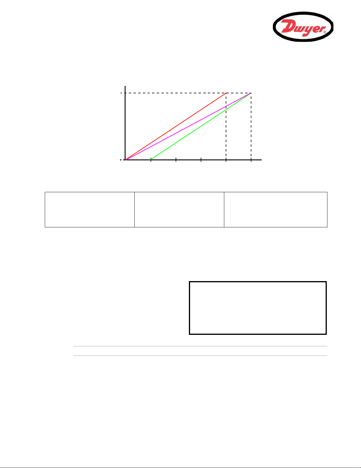
4 8 12 16 20

max

Flow (gal/min)

I (mA)

min

[0-16 mA scale]

[0-20 mA scale]

[4-20 mA scale]

Flow rate

maxFmin

–

------------------------------------------- F

min

Flow rate

maxFmin

–

------------------------------------------- F

min

Flow rate

I 4–F

maxFmin

–

16

--------------------------------------------------------- F

min

PULSE OUTPUT * *

Pulse output is ON

Flow units : gallons Output : Off Vol per pulse : 10.00 Pulse width (ms) : 10 Exit

How to convert the measured current to flow rate

Assume the maximum flow rate is F

To calculate the flow rate (gal/min) for a measured current I(mA) then:

(gal/min) and the minimum flow rate F

max

is ‘0’ (gal/min), as shown.

min

0-20 mA 0-16 mA 4-20 mA

3.4.2 Pulse output

Pulse output configuration

Two parameters can be configured from the PULSE OUTPUT menu:

• Volume of fluid per pulse.

• Pulse width.

1. With the instrument operating in the FLOW READING mode, press the Pulse function key

to access the PULSE OUTPUT screen.

2. Ensure that the Output is Off.

3. Select Vol per pulse and press ENTER.

4. Enter the required value. (In the example shown, a pulse is produced for every 10 gallons of flow).

Note: The

5. Select a Pulse width (in ms) to suit the particular application – e.g. electro-mechanical counter. Refer to the manufacturer’s data sheet for the minimum pulse width.

6. Select Exit and press ENTER to return to the FLOW READING screen.

Vol per pulse

can only be changed if the

Pulse Output

Off

Find Quality Products Online at: sales@GlobalTestSupply.com

www.GlobalTestSupply.com

How to turn the pulse output OFF/ON

PULSE OUTPUT * *

Pulse output is ON

Flow units : gallons Output : Off Vol per pulse : 10.00 Pulse width (ms) : 10 Exit

FLOW READING OPTION DD-MM-YY HH:MM:SS

Data review Zero Cutoff (m/s) : 0.010 Set zero flow (m/s) : 0.000 Damping (secs) : 10 Totaliser : Run Reset +Total

7. With the instrument operating in the FLOW READING mode, press the Pulse function key

to access the PULSE OUTPUT menu.

8. Select Output and press ENTER.

9. Select On and press ENTER.

10. A Pulse output is ON message will appear in

the second line of the display.

11. S ele ct Exit and press ENTER to return to the FLOW READING screen.

3.4.3 Alarm outputs

The UFB provides two programmable alarm outputs that are interfaced by opto-isolated relays. The relay contacts are rated at a 48 V (maximum voltage across the open contacts) and 500 mA (maximum continuous current through the closed contacts).

The two alarm outputs can be individually configured to operate in one of five modes:

• Activate at a predefined Low or High flow rate.

• Activate when a specified Volume is measured.

• Activate if a signal error is detected – either due to poor signal strength or complete signal loss.

• Alarm Test mode.

• Pulse Frequency output.

Alarm settings selection

1. To access the The ALARM SETTINGS menu select Alarm Settings from the FLOW READING OPTION menu and press ENTER.

2. The ALARM SETTINGS screen should be displayed, as shown below. This screen shows two parameters (Mode and Limit) that can be individually set for Alarm 1 and Alarm 2.

3: Operating Procedures

Find Quality Products Online at: sales@GlobalTestSupply.com

www.GlobalTestSupply.com

3: Operating Procedures

ALARM SETTINGS * *

Alarm1 Mode Alarm1 Level : <value> Alarm2 Mode Alarm2 Level : <value> Exit Alarm1 ON Alarm2 ON

ALARM1 MODE * *

Off Low High Volume On Flow Error Alarm Test

Frequency

ALARM SETTINGS * *

Alarm1 Mode Alarm1 Level : <value> Alarm2 Mode Alarm2 Level : <value> Exit Alarm1 ON Alarm2 ON

Alarm configuration

1. To setup Alarm 1, select Alarm1 Mode and

press ENTER. This will access the ALARM1 MODE menu screen (shown below).

2. Scroll down the menu to the required alarm

operating mode and press ENTER.

3. This will return you to the ALARM SETTINGS

menu.

4. If the selected mode is Low, High or Volume,

select Alarm1 Level, enter an appropriate value then press ENTER to set the alarm operating point (see below).

High or Low limit values

If High or Low limits are selected, the value entered in the ALARM SETTINGS menu must be in the range

-9999 to +9999. This value is in the units previously selected (e.g. gal/min). The default value is +9999.

Volume limit values

If VOL limit is selected, the value entered in the ALARM SETTINGS menu must be in the range

-3,999,999,999.99 to +3,999,999,999.99. This value will be in the units previous selected (e.g. liters, m3, gals) The default value should be +3,999,999,999.99.

Alarm Test

1. Select Alarm Test and press ENTER in the Alarm1 MODE menu to test that Alarm1 can be activated.

2. Select Alarm Test and press ENTER in the Alarm2 MODE menu to test that Alarm2 can be activated.

Pulse Frequency

When Frequency is selected, a variable frequency pulse proportional to the flow rate can be output at the ALARM 1 or ALARM 2 outputs. When this feature is used, the Max Pulse freq (Hz) and Flow at Max Frequency must be set in the FLOW READING OPTION menu.

Find Quality Products Online at: sales@GlobalTestSupply.com

www.GlobalTestSupply.com

3: Operating Procedures

FLOW READING OPTION DD-MM-YY HH:MM:SS

Data review Zero Cutoff (m/s) : 0.010 Set zero flow (m/s) : 0.000 Damping (secs) : 10 Totaliser : Run Reset +Total

ALARM SETTINGS * *

Alarm1 Mode Alarm1 Limit : <value> Alarm2 Mode Alarm2 Limit : <value> Exit Alarm1 ON Alarm2 ON

ALARM1 MODE * *

Off Low High Volume On Flow Error Alarm Test

Frequency

Resetting an alarm

When either Alarm1 or Alarm2 is activated, the appropriate relay will be held in the closed position until:

• The activation condition is removed, or

• The Alarm is reset.

Both Alarm1 and Alarm2 can be reset by using one of the following procedure:

1. Access the The ALARM SETTINGS menu by selecting Alarm Settings from the FLOW READING OPTION menu, and press ENTER.

2. The ALARM SETTINGS screen should be displayed, as shown below.

Alarm configuration

1. To reset Alarm 1, select Alarm1 Mode and press ENTER. This will access the ALARM1 MODE menu screen (shown below).

2. Select Off from the menu and press ENTER.

3. This should de-activate the alarm.

Find Quality Products Online at: sales@GlobalTestSupply.com

To re-arm the alarm you must ensure that the activation condition is removed and then reconfigure the Alarm Mode as described above on page 30.

www.GlobalTestSupply.com

3: Operating Procedures

FLOW READING OPTION * *

Data review Zero Cutoff (m/s) : 0.010 Set zero flow (m/s) : 0.000 Damping (secs) : 10 Totalizer : Stall Reset +Total

FLOW READING OPTION * *

Zero Cutoff (m/s) : 0.00 Set zero flow (m/s) : 0.00 Damping (secs) : 10 Totalizer : Run Reset +Total Reset –Total

FLOW READING * *

Qxx.xx%

Signal

gal/min

+Total: 300.0 gallons –Total: 0.00 gallons

12.34

3.5 How to Measure Totalized Flows (manually)

The basic measurement indicated on the FLOW READING screen is the instantaneous flow rate, which in some applications may vary over a period of time. Average flow rates are therefore often required in order to get a better understanding of an application’s true performance. This is simply achieved by noting the total flow over a specific period (for example 30-60 minutes) and then calculating the average flow rate over that period of time.

1. Press the Options key to access the FLOW

READING OPTION screen shown.

2. If the Totalizer is indicating Run, select it

and change it to Stall. Press ENTER.

3. Select Reset +Total and press ENTER.

4. Press ENTER on the subsequent screen to

accept the reset.

5. Press ENTER again to return to the FLOW

READING OPTIONS menu.

6. Select Reset –Total and press ENTER.

7. Press ENTER on the subsequent screen to

accept the reset.

8. Press ENTER again to return to the FLOW

READING OPTIONS menu.

9. Note and record the current time.

10. Select Totalizer and change it to Run. Press

ENTER.

Note: the totalizers begin to count up as soon as Totalizer is set to Run.

11. Scroll down and select Exit to return to the

FLOW READING screen which will now indicate

the instantaneous flow together with the totalized flow.

Note that in some installations the measured flow can be in either direction. When this is the case, the upstream flow is shown separately in the –Total field.

Calculating the average flow

To calculate the average flow, wait for the allotted monitoring period to expire then divide the indicated total flow by the time taken. This will give you the average flow in m/s, galls/hour or whatever units you select.

Note that in a bi-directional flow situation you must calculate the difference between the indicated positive and negative flow totals before carrying out the average flow rate calculation.

How to stop the totalizer temporarily

If you want to stop the totalizer temporarily for operational reasons, set the Totalizer option to Stall in the FLOW READING OPTIONS screen as described above. This will stop the totalizer operation without affecting its

current values.

Find Quality Products Online at: sales@GlobalTestSupply.com

www.GlobalTestSupply.com

3.6 Display of totalizers

FLOW READING OPTION DD-MM-YY HH:MM:SS

Data review Zero Cutoff (m/s) : 0.010 Set zero flow (m/s) : 0.000 Damping (secs) : 10 Totaliser : Run Reset +Total

3: Operating Procedures

1. To change the display of the totalizers,

select the Select Totals menu item from the FLOW READING OPTION menu.

2. The display of the totals on the FLOW

READING screen is controlled by this menu.

3. Select one, both or no totals to be displayed.

The default is the display of the +Total.

4. Press the ENTER key.

Note: This menu selection only affects the Display of the totalizer. Unless the totalizers are stalled, the recorded volume will still be incremented and the totals will be logged irrespective of the display setting.

3.7 Setting the Chiller Options

When there is a significant change in flow rate in a chiller system the acoustic properties of the fluid can change such that the signal is temporarily lost or a false flow reading is obtained. Under these conditions the normal action of the UFB system is to go to a fault state on both the flow reading and the current output, which may be undesirable on a short term loss of signal. This potential problem can be overcome by selecting a suitable setting in the Chiller Options sub-menu and entering an appropriate value for the Chiller Delay option, as follows.

1. Press the Options key to access the FLOW READING OPTION screen shown.

2. Scroll down and select Chiller Options and press ENTER. This will open the CHILLER

OPTIONS screen.

FLOW READING OPTION * *

Off Both +Total

-Total

Find Quality Products Online at: sales@GlobalTestSupply.com

www.GlobalTestSupply.com

3: Operating Procedures

CHILLER OPTIONS DD-MM-YY HH:MM:SS

Off Zero Negative Hold No Reset

FLOW READING OPTION DD-MM-YY HH:MM:SS

Data review Zero Cutoff (m/s) : 0.010 Set zero flow (m/s) : 0.000 Damping (secs) : 10 Totaliser : Run Reset +Total

3. Select the required option, as detailed below.

4. Press ENTER to apply the change.

Off

No change in response to a lost signal. This is the default value.

Zero

Disables the fault condition, and the system’s outputs act as if the flow reading has gone to zero.

Negative

A false negative flow reading may be generated as a result of the poor conditions in the pipe; but with this option selected any negative readings are displayed as zero flow.

Hold

With this option selected, the flow reading will remain at the last valid value for a time period set by the Chiller Delay (s). After which time the normal fault condition will occur.

No Reset

Used to prevent the system changing the flow reading setup when the fluid conditions change and then, after a delay when the conditions return to normal, changing back to the original setup. This may reduce the time that the poor conditions affect the performance of the instrument, by not reacting to a short term fault condition.

3.7.1 Setting the Chiller Delay

If a signal fault occurs when the CHILLER OPTION is set to Hold, the selected Chiller Delay determines how long, in seconds, the flow reading is held at the last valid value before it reverts to a fault condition.

1. Press the Options key to access the FLOW

READING OPTION screen shown.

2. Scroll down and select Chiller Delay then

press ENTER.

3. Using the numerical keypad, enter a Chiller

Delay value between 0 (default) and 9999 seconds.

4. Press ENTER to apply the change.

Find Quality Products Online at: sales@GlobalTestSupply.com

5. The applied Chiller Delay value will now be

displayed.

www.GlobalTestSupply.com

3.8 Operation with an Energy Meter

T

FLOW READING OPTION * * Data review Zero Cutoff (m/s) : 0.010 Set zero flow (m/s) : 0.000 Damping (secs) : 10 Totalizer : Run Reset +Total

ALARM SETTINGS * *

Alarm1 Mode Off Alarm1 Level : Alarm2 Mode Off Alarm2 Level : Exit

The UFB can be operated with an energy meter which allows accumulated energy measurements to be made. In this configuration, one temperature sensor is fitted to the output pipe (hot side) and another to the return pipe

(cold side). The temperature difference ( = Thot - Tcold), measured by the energy meter, together with the

pulse input from the UFB, allows the energy meter to calculate and display the accumulated energy absorbed by the heating system.

3.8.1 Pulse output

When working with an energy meter, the UFB normal pulse output is not used. Instead, a pulse whose frequency is proportional to the flow rate is independently generated and output on ALARM1 or ALARM2 outputs. This gives a more stable reading than the pulse ‘packets’ that would normally be produced.

3.8.2 Configuring the UFB

Configure the UFB frequency pulse output using the following procedure:

1. From the FLOW READING screen, press the

Options key to select the FLOW READING OPTIONS menu, shown here.

3: Operating Procedures

Note: You may need to enter the password first.

2. Scroll down to Alarm Settings and press ENTER to select the ALARM SETTINGS menu.

3. Select Alarm 1 Mode and press ENTER to select the ALARM1 MODE menu shown below:

Find Quality Products Online at: sales@GlobalTestSupply.com

www.GlobalTestSupply.com

3: Operating Procedures

ALARM1 MODE * *

Off Low High Volume On Flow Error Alarm Test

Frequency

ALARM SETTINGS * *

Alarm1 Mode Frequency Alarm1 Level : Alarm2 Mode Off Alarm2 Level : Exit

FLOW READING OPTION * *

Data review Zero Cutoff (m/s) : 0.010 Set zero flow (m/s) : 0.000 Damping (secs) : 10 Totalizer : Run Reset +Total

Reset –Total Calibration factor : 1.000 Roughness factor : 0.010 Alarm Settings : Max Pulse Freq (Hz) : 10.00 Flow at Max Frequency : 200.00 Calculated Pulse Value: 20.0 Diagnostics Select Totals : +Total Chiller Delay : 0 Chiller Options : Off Exit

4. Scroll down to Frequency and press ENTER.

5. This returns to the ALARM SETTINGS menu

which will indicate Frequency on the Alarm 1 Mode field as shown below.

6. Select Exit to return to the FLOW READING

OPTIONS menu.

7. Scroll down to select Max Pulse Freq.

(Hz) and press ENTER.

8. Enter the required maximum pulse frequency,

e.g. 10Hz or 200Hz and press ENTER.

9. Select Flow at Max Frequency and press

ENTER.

10. Enter the maximum flow rate (in liters per

second) corresponding to 10Hz (or 200Hz) and press ENTER.

11. Th e Calculated Pulse Value indicates

the relationship between the frequency and the flowrate. This is a non-editable value.

12. Select Exit and press ENTER to return to the

FLOW READING screen. The message ‘Frequency Pulse is ON’ should now be displayed on the status line of the display (line 2).

Find Quality Products Online at: sales@GlobalTestSupply.com

Note: ALARM 2 can be used instead of ALARM 1. The procedure is identical except that Alarm 2 Mode is selected and the frequency pulse output is connected to ALARM2+ and ALARM2-.

www.GlobalTestSupply.com

4: Maintenance & Repair

WARNING

4.1 Introduction

This instrument does not contain any user-serviceable parts. The following notes are provided as a guide to general equipment

Do not disassemble this unit.

Return the unit to an approved service agent or place of purchase for

further advice.

4.2 General care

The following notes are provided as a guide to general equipment care.

1. Ensure the unit is disconnected from the mains, then wipe the exterior of the instrument with a clean, damp cloth or paper towel. Do not use a solvent-based cleaning fluid on the instrument as it could damage the instrument surface.

2. Ensure all cables and connectors are kept clean and free from grease or contaminants. Connectors may be cleaned with a general purpose cleaner if necessary.

3. Avoid the use of excessive grease/ultrasonic couplant on the sensors as this may impair the performance of the equipment. Excessive grease/couplant can be removed from the sensors and transducer holders using an absorbent paper towel and a general purpose solvent cleaner.

4. We recommend that the ultrasonic couplant is replaced on the sensors every 6 months, especially on pipes where the application is too hot to touch. If the signal level drops below 30% this is also an indication that the sensors need re-greasing.

5. Regularly check all cables/parts for damage. Replacement parts are available from Dwyer.

6. Ensure the person who services your instrument is qualified to do so. If in doubt, return the instrument to Dwyer with a detailed report on the nature of any problem.

7. Ensure that suitable precautions are taken when using any materials to clean the instrument/sensors.

8. If the instrument was supplied with dust or dirt caps make sure they are re-fitted when the instrument is not in use.

4: Maintenance & Repair

4.3 Warranty / Return

Refer to “Terms and Condition of Sales” in our catalog and on our website. Contact Customer Service to receive a Return Goods Authorization number before shipping the product back for repair. Be sure to include a brief description of the problem plus any additional application notes,

Find Quality Products Online at: sales@GlobalTestSupply.com

www.GlobalTestSupply.com

5: Troubleshooting

5.1 Overview

If you have a problem with your flow monitoring system it can be due to any of the following:

Faulty instrument

Blank instrument display:

• Loss of power supply to the instrument.

• Internal power supply fuse ruptured.

Scrambled instrument display:

• Reboot the instrument by temporarily disconnecting its power supply.

Incorrect setup

A low, or zero, signal could be caused by incorrect set-up such as:

• Incorrect site data entered into the instrument.

• Incorrect or non-matching ultrasonic transducers selected for use.

• Incorrectly fitted transducers – lack of couplant applied, incorrect spacing, insecure attachment.

• Poor connections between the probes and the instrument.

Application problem

If you are certain that the instrument is healthy and suitably set-up for the current site; and the probes are properly assembled and fitted correctly, there could be an application problem concerned with the site.

Check such conditions such as:

Poor pipe outer surface quality

• Uneven surface preventing good surface contact with the transducer.

• Flaking paint (should be removed).

• Variable air gap in concrete-covered pipes affecting the ultrasonic signal quality.

Poor internal pipe construction

• Rough internal pipe walls affecting fluid flow (see roughness factor).

• Internal welds positioned in the transducer signal path affecting the signal quality.

• The ‘drippings’ in galvanized-dipped pipes or other irregularities interfering with the signal path.

Incorrect probe location

• Transducers located too close to bends or valves, disturbing the flow profile.

• Transducers located too close to insertion probes, disturbing the flow profile.

• For horizontal pipework, transducers should not be positioned on the top of the pipe.

Poor fluid conditions within the pipe

• Fluid contains bubbles, high particle density or sludge.

• Air in the top of the pipe.

Low fluid flow within the pipe

• Pipe obstructions.

• Malfunctioning valve not opening fully (or closed inadvertently).

Liquid content problems

•

Multiple liquid contents do not comply accurately to expected sound speed criteria.

Find Quality Products Online at: sales@GlobalTestSupply.com

www.GlobalTestSupply.com

• Very hot pipe almost turns water to steam and therefore exhibits the wrong speed characteristics –could

Is the display blank?

Loss of power supply.

Confirm power supply availability.

(note: if using 24V power supply,

the internal fuse should reset

when power is removed)

Turn instrument OFF/ON.

If the display is still scrambled/

hung up, return the instrument for

repair.

Yes

Is the display scrambled or

hung up?

Yes

Measurement differs from expected value.

Unstable measurements. No (or poor) sig nal.

Problem probably due to non-constant fl uid flow.

Check the following:

- the pipe data has been entered correctly.

- the fluid type has been entered correctly.

- the correct transducer type has been se lec te d .

- the pipe diameter is within specifications of the selected transducers.

- the pipe is completely full.

- the pipe surface is not corroded, or protective surface loose.

- no particles in the fluid.

Ensure the temperature is set correctly.

Ensure that the transducer cabl es are connected

correctly.

Ensure transducers are posi tioned in accordance

with the recommended distance from bends etc.

Ensure flow velocity >0.01m/s.

Ensure that sufficient acoustic couplant has been

applied to the transducers.

If triple refl ex mode is selected, try selecting

double or single reflex instead.

START

Are any

status messages

shown?

Note any active messages.

Refer to the message table in this

chapter to interpret the message

and view suggested response.

Yes

be due to reduced pipe pressure.

• Flashover – liquid turns into a gas because of lower than required pressure.

5.2 General Troubleshooting Procedure

5: Troubleshooting

Find Quality Products Online at: sales@GlobalTestSupply.com

Figure 5.1 Troubleshooting chart

www.GlobalTestSupply.com

5: Troubleshooting

5.3 Warning and Status Messages

FLOW RATE ERRORS

ERR:No flow signal Interpretation: This message appears when the transducers cannot send or receive

signals to each other.

Response: Check that all cables are connected, transducers are on the pipe

correctly with sufficient couplant on the face. This condition could also be due to a partially empty pipe, aerated liquid, particulate content too high or when the condition of the pipe being measured is poor.

Flow signal is poor Interpretation: This warning appears when the signal is lower than 25%.

Response: This could be due to an application problem, a poor quality pipe – see

also the conditions for No flow signal (above). Check for sufficient couplant.

ERR:Zero cut-off! Interpretation: You have entered an out-of-range value in the Zero cutoff field

in the Options menu.

Response: Enter a valid number.

Totalizer beyond maximum! Interpretation: The totalizer has overflowed its maximum count. The counter will

roll-over and restart from zero but this message alerts you to the fact.

Response: Reset the totalizer as described in Paragraph 3.5.

PULSE ERRORS

ERR:Pulse output! Interpretation: The flow rate exceeds the capability of the pulse output – i.e. too

many pulses per second are required than can be achieved.

Response: Narrow the pulse width time or increase the volume per pulse, as

described in Paragraph 3.4.2.

ERR:Pulse volume! Interpretation: You have entered an out-of-range value in the Pulse volume

error field in the PULSE OUTPUT menu – see Paragraph 3.4.2.

Response: Enter a valid number.

ERR:Pulse width! Interpretation: You have entered an out-of-range value in the Pulse width

error field in the PULSE OUTPUT menu – see Paragraph 3.4.2.

Response: Enter a valid number.

Find Quality Products Online at: sales@GlobalTestSupply.com

www.GlobalTestSupply.com

5: Troubleshooting

4-20mA ERRORS

Calibration 20mA Error! NOTE: The 4 to 20 mA output is calibrated before the instrument leaves the factory

and should not require further adjustment.

Interpretation: You have adjusted the DAC outside its accepted range when

calibrating the 20 mA signal output.

Response: Re-calibrate the 4 to 20 mA output – see Paragraph 3.4.1.

Calibration 4mA Error! NOTE: The 4 to 20 mA output is calibrated before the instrument leaves the factory

and should not require further adjustment.

Interpretation: You have adjusted the DAC outside its accepted range when

calibrating the 4 mA signal output.

Response: Re-calibrate the 4 to 20 mA output – see Paragraph 3.4.1.

SET-UP ERRORS

ERR:Pipe OD range! Interpretation: You have entered an out-of-range value for the pipe outside

diameter dimension – i.e. larger or smaller than the unit or sensor can be used on.

Response: Enter a valid number.

ERR:Wall thk. range! Interpretation: You have entered an out-of-range value for the pipe wall thickness

dimension – accepted range is 0.04 to 3 inches (1 to 75 mm).

Response: Enter a valid number.

ERR:Lining thick. range! Interpretation: You have entered an out-of-range value for the lining thickness

dimension – acceptable range is 0 to 1 inch (0 to 25 mm).

Response: Enter a valid number.

ERR:Temperature range! Interpretation: You have entered an out-of-range value for the fluid temperature.

Accepted temperature range -4°F to +392°F (-20°C to +200°C).

Response: Enter a valid number.

ERR:Invalid Date or Time! Interpretation: The entered Date or Time is invalid, or when setting up ‘timed’ data

logging the Stop time is set earlier than the Start time.

Response: Enter a valid Date and Time.

ERR:Invalid Sensor or Mode Interpretation: The selected temperature is higher than the maximum allowed for

the sensor type.

Response: Change the temperature.

Mode: Err Type Interpretation: The selected sensors are invalid and the mode cannot be verified.

Response: Choose a mode that gives a non-zero separation distance.

Find Quality Products Online at: sales@GlobalTestSupply.com

www.GlobalTestSupply.com

5: Troubleshooting

5.4 Diagnostics Display

This feature is designed for advanced users and is intended to provide information that will aid the user to diagnose problems – e.g. no signal strength.

When operating in the FLOW READING mode you can access a diagnostics screen by pressing the Options function key and then selecting Diagnostics from the FLOW READING OPTIONS screen. This will display the operating values for the following parameters.

Calculated time (µs)

This is a value the instrument predicts will be the time in µsecs that it should take for the acoustic wave to propagate across a particular pipe size. This value is ascertained from the data entered by the user. i.e. Pipe size, material, sensor set etc.

Actual time (µs)

This is the value the instrument measures as the time taken for the acoustic wave to propagate across the pipe. It is used to see if the signal is being taken from the burst, at the correct time to get the strongest signal. This value is normally a few µs below the calculated µs value. If, however, this value is much greater than the calculated time, there is a problem with the set-up.

Flow (m/s)

This displays flow velocity in m/s to 3 decimal places.

Signal strength

This is the averaged value of Signal and should be a value between 800 and 1600 – where 800 is approximately 50%, and 1600 is approximately 100%.

Gain

Gain values are typically in the range 600 to 850.

Switches

Typical Switches values are None and *10. On small pipes (and when using the test block) the value should be None. A Switch value of *100 indicates poor sensor set-up or poor connections.

UP/DN time difference

The difference in transit times between the upstream and downstream signals due to the fluid flow.

Fluid propagation rate

This is the sound speed of the fluid calculated using the data entered by the user.

Sensor separation

The same value as displayed in the setup screen.

Find Quality Products Online at: sales@GlobalTestSupply.com

www.GlobalTestSupply.com

6: Options

6.1 Large Pipe Diameter Transducers

Type ‘D’ transducers are available for use with pipe diameters in the range 59 to 197 inches (1500 to 5000 mm), operating over the temperature range -4°F to +176°F (-20°C to +80°C). The type ‘D’ transducer kit is supplied in a separate case and includes the sensors together with ratchet straps and transducer holders for attaching to the pipe.

6.2 Transducer Holder Options

The standard method of securing the transducer holder to the pipe is by stainless steel banding. However, optional end plates are available to allow fixing by chain.

6.3 Extended Signal Cable Options

Standard transducer cables are 16.5 ft. (5 m) in length with 33 ft. (10 m) cables being optionally available. Where, for operational reasons, it is not possible to mount the instrument this close to the sensors, bespoke cables of up to 328 ft. (100 m) can be provided. Consult Dwyer for further information and availability.

6: Options

Find Quality Products Online at: sales@GlobalTestSupply.com

www.GlobalTestSupply.com

7: Specification

GENERAL

DSP Measurement Technique: Transit time.

Timing Resolution: 50 pico-second, continuous signal level indication on display.

Flow Velocity Range: Minimum Velocity 0.33 ft/s; Max Velocity 33 ft/s: Bi-directional.

Turn Down Ratio: 200:1

Accuracy: ±0.5% to ±2% of flow reading for flow rates >0.66 ft/s and Pipe OD >3.0 in (75 mm).

Repeatability: ±0.5% of measured value or ±0.66 ft/s whichever is the greater.

Reynolds Number Correction: Flow velocity corrected for Reynolds number over entire velocity range.

Response Time: < 500 ms depending on pipe diameter.

Selectable Flow Units: VELOCITY: m/sec, ft/sec.

Selectable Volume Units: US gallons, gallons, barrels (oil), liters, m³.

Total Volume: 12 Digits - forward and reverse.

APPLICABLE FLUID TYPES

Fluid Condition: Clean liquids or oils that have less than 3% by volume of particulate content. Applications include

APPLICABLE PIPE TYPES

Pipe Materials: Any sonic conducting medium such as Carbon Steel, Stainless Steel, Copper, UPVC, PVDF,

Pipe Dimension (outside diameter): Min 0.5

±3% of flow reading for flow rates >0.66 ft/s and Pipe OD in range 0.5 to 3.0 in (13 to 75 mm). ±6% of flow reading for flow rates <0.66 ft/s.

VOLUME: L/s, L/min, L/h, gal/s gal/min, gal/h, USgals/s, USgals/min, USgals/h, Barrel/h, Barrel/ day, m³/s, m³/min, m³/h.

river water, sea water, potable water, demineralized water, glycol/water mix, hydraulic systems and diesel oil.

Concrete, Galvanized Steel, Mild Steel, Glass, Brass. Including Lined Pipes - Epoxy, Rubber, Steel, Plastic.

inch (13 mm); Max 197 inches (5000 mm) with D sensor set.

Pipe Wall Thickness: 0.04 to 3.0 inches (1 to 75 mm).

Pipe Lining: Applicable pipe linings include Rubber, Glass, Concrete, Epoxy, Steel.

Pipe Lining Thickness: 0.0 to 1.0 inches (0 to 25 mm).

Pipe Wall Temperature Range: Standard sensor operating temperature is -4°F to +275°F (-20°C to +135°C).

Find Quality Products Online at: sales@GlobalTestSupply.com

www.GlobalTestSupply.com

7: Specification

TRANSDUCER SETS

Standard: Temperature Range -4°F to +275°F (-20°C to +135°C).

'A-ST' (standard) 0.5 to 4.5 inches (13 to 115 mm) pipe OD (2 MHz). 'B-ST' (standard) 2 to 79 inches (50 to 2000 mm) pipe OD (1 MHz). Protection: IP54.

Optional: 'D' 59 to 197 inch (1500 to 5000 mm) pipe OD (0.5 MHz), with an operating temperature range of

-4°F to +176°F (-20°C to +80°C).

LANGUAGES

Standard Supported Languages: English, French, German, Italian, Spanish, Portuguese, Russian, Norwegian, Dutch, Swedish.

OUTPUTS

Current Output:

No. Channels Format: Resolution: Error Currents: Isolation: Maximum Load:

1 4 to 20 mA, 0 to 20 mA, 0 to 16 mA.

0.1% of full scale. Any between 0 to 26 mA. 1000 V Opto-isolated from unit. 620 Ohms.

Pulse Output TTL:

Number Available: Isolation: Pulse Repetition Rate: Pulse Width: Max Current: Max Voltage:

Alarms:

Number of Channels Available: Isolation: Relay Contact Mode:

Alarm Functions:

Frequency output: Max Current: Max Voltage:

1 – Opto-isolated MOSFET relay. 1500 V opto isolated from unit. User programmable from 1 to 250 pps. User programmable from 2 ms to 500 ms. 500 mA. 48 V.

2 off opto-isolated MOSFET relay. 1500 V opto isolated from unit. N/O when switching condition is False. Closed when switching condition is True. The two relays can be configured to operate when:

Maximum 200 Hz. 500 mA. 48 V.

ELECTRICAL

Supply Voltage:

Mains Input Voltage: 86 to 264 Vac

Mains Input Frequency: 47 to 63 Hz

• a predefined

• a specified

• a signal Error condition occurs.

• manual alarm test.

• pulse frequency.

MINimum or MAXimum flow rate is exceeded.

VOLume is measured.

Power Consumption: 10.5 W.

Alternative Input Supply: 24 V(ac/dc), 1 A max. (The 24 Vac supply must be isolated from earth.)

Find Quality Products Online at: sales@GlobalTestSupply.com

www.GlobalTestSupply.com

7: Specification

MECHANICAL

Enclosure:

Material: ABS and aluminium.

Dimensions: 9 x 7 x 4.7 inches.

Weight: 2.65 lb.

Protection: IP65.

Fixing: Wall mountable.

Keypad:

No. Keys: 15 key tactile feedback membrane keypad.

Display:

Format: 240 x 64 pixel graphic display, high contrast black-on-white, with backlight.

Viewing Angle: Min 30°, typically 40°.

Active Area: 5.0 in (W) x 1.3 in (H).

Overlay: Standard English, Optional overlays available.

ENVIRONMENTAL

Operating Temperature: -4°F to +122°F (-20°C to +50°C).

Storage Temperature: -13°F to +167°F (-25° to +75°C).

Operating Humidity: 90% RH MAX at +122°F.

APPROVALS

Safety: BS EN 61010-1:2001.

EMC: BS EN 61326 - 1:2006, BS EN 61326-2-3:2006.

Environmental: BS EN 60068-1:1995, BS EN 60068-2-1:2007, BS EN 60068-2-2:2007.

SHIPPING INFORMATION

Box Dimensions: 18.9 in x 12.6 in x 6in.

Weight: 9.9 lb.

Volumetric Weight: 8.4 lb.

Dwyer reserve the right to alter any specification without notification.

Find Quality Products Online at: sales@GlobalTestSupply.com

www.GlobalTestSupply.com

Dwyer Instruments UFB-222, UFB-122, UFB-223, UFB-123 User manual

Specifications and Main Features

Frequently Asked Questions

User Manual

1: General Description

1.1 Introduction

1.2 Principles of Operation

1.3 Supplied Hardware

UFB Standard equipment

UFB Optional equipment

1.4 UFB Instrument

1.4.1 Connections

1.4.2 Keypad

1.4.3 Power supply

Mains supply

24V Supply

Power failure

2: Installation

2.1 Safety Precautions and Warnings

2.2 Installing the UFB Instrument

2.2.1 Positioning the instrument

2.2.2 Mounting the instrument

2.2.3 Connecting the instrument

Control & monitoring cables

Power connections

2.3 Installing the Ultrasonic Transducers

2.3.1 Transducer positioning

Preparation

2.3.2 Transducer attachment

2.3.3 Attaching the guide rail to the pipe

2.3.4 Fitting the transducers

2.3.5 Transducer attachment (diagonal mode)

3: Operating Procedures

3.1 Setting-up the Instrument

3.1.1 Using the instrument for the first time

Initial user language selection

The MAIN MENU screen

3.1.2 Changing the user language

3.2 Using the Quick Start Menu

Entering the site data

Selecting the operating mode

Password Control

Attaching and connecting the transducers

Taking a flow reading

Flow monitoring

3.3 Instrument Calibration

3.3.1 Adjusting the zero cut-off

3.3.2 Adjusting the set zero flow offset

3.3.3 Adjusting the calibration factor

3.3.4 Adjusting the roughness factor

3.3.5 Adjusting the damping factor

3.4 Outputs

3.4.1 Current output

How to turn the 4 to 20 mA output OFF/ON

4 to 20 mA Signal calibration and ranging

Signal calibration

4-20mA Signal scaling

How to convert the measured current to flow rate

3.4.2 Pulse output

Pulse output configuration

How to turn the pulse output OFF/ON

3.4.3 Alarm outputs

Alarm settings selection

Alarm configuration

Resetting an alarm

Alarm configuration

3.5 How to Measure Totalized Flows (manually)

Calculating the average flow

How to stop the totalizer temporarily

3.6 Display of totalizers

3.7 Setting the Chiller Options

3.7.1 Setting the Chiller Delay

3.8 Operation with an Energy Meter

3.8.1 Pulse output

3.8.2 Configuring the UFB

4: Maintenance & Repair

4.1 Introduction

4.2 General care

4.3 Warranty / Return

5: Troubleshooting