Dionex MSQ User Manual

Download

Page 1

MSQ

Document No. 031871

Hardware

Revision 02

October 2003

™

Page 2

This publication is protected by federal copyright law. No part of this publication may be copied or distributed, transmitted, transcribed, stored in a retrieval system, or transmitted into any human or computer language, in any form or by any means, electronic, mechanical, magnetic, manual, or otherwise, or disclosed to third parties without the express written permission of Dionex Corporation, 1228 Titan Way, Sunnyvale, California 94088-3603 U.S.A.

DISCLAIMER OF WARRANTY AND LIMITED WARRANTY

THIS PUBLICATION IS PROVIDED “AS IS” WITHOUT WARRANTY OF ANY KIND. DIONEX CORPORATION DOES NOT WARRANT, GUARANTEE, OR MAKE ANY EXPRESS OR IMPLIED REPRESENTATIONS REGARDING THE USE, OR THE RESULTS OF THE USE, OF THIS PUBLICATION IN TERMS OF CORRECTNESS, ACCURACY, RELIABILITY, CURRENTNESS, OR OTHERWISE. FURTHER, DIONEX CORPORATION RESERVES THE RIGHT TO REVISE THIS PUBLICATION AND TO MAKE CHANGES FROM TIME TO TIME IN THE CONTENT HEREINOF WITHOUT OBLIGATION OF DIONEX CORPORATION TO NOTIFY ANY PERSON OR ORGANIZATION OF SUCH REVISION OR CHANGES.

TRADEMARKS

Chromeleon is a registered trademark of Dionex Corporation. Cone Wash, M-Path, MSQ, and Xcalibur are trademarks of Thermo Electron Corporation. Microsoft is a registered trademark of Microsoft Corporation. Q-tip is a trademark of Chesebrough-Pond’s, Inc. Teflon, Vespel, and Viton are registered trademarks of E.I. du Pont de Nemours and Company.

PRINTING HISTORY

Revision 01, July 2002 Revision 02, October 2003

The products of Dionex Corporation are produced under ISO 9001 accredited quality management systems.

Published by Technical Publications, Dionex Corporation, Sunnyvale, CA 94086.

Page 3

Chapter 1

Introducing the MSQ 1.

Introducing the MSQ.................................................................................................................1-i

Introduction ....................................................................................................................................1-1

System Overview............................................................................................................................1-2

What Is Mass Detection?...................................................................................................1-4

Exterior Features of the MSQ............................................................................................1-5

The Source–An Introduction to API Techniques ...........................................................................1-8

Electrospray.......................................................................................................................1-9

Atmospheric Pressure Chemical Ionization.....................................................................1-13

Source Fragmentation......................................................................................................1-16

Cone Voltage Ramping ...................................................................................................1-18

Polarity Switching ...........................................................................................................1-19

Application of API Techniques .......................................................................................1-20

The Self-Cleaning Source: Cone Wash ........................................................................................1-23

Introduction .....................................................................................................................1-23

Functional Description ....................................................................................................1-24

The Reference Inlet System..........................................................................................................1-25

Introduction .....................................................................................................................1-25

Functional Description ....................................................................................................1-25

The Mass Analyzer and Detector .................................................................................................1-26

The Vacuum System.....................................................................................................................1-27

The Data System...........................................................................................................................1-28

Software...........................................................................................................................1-28

Raw Data .........................................................................................................................1-30

Raw Data Types...............................................................................................................1-31

____________________________MSQ Hardware Manual _____________________________ 1-i

Page 4

Introducing the MSQ Introduction ____________________________________________________________________________

1-ii____________________________ MSQ Hardware Manual ____________________________

Page 5

Introducing the MSQ

___________________________________________________________________________ Introduction

Introduction

The MSQ™ MS detector has been specifically designed and engineered for liquid chromatographic detection using Atmospheric Pressure Ionization (API) and Mass Spectrometry (MS) technology. These technologies can provide sensitive and selective detection of organic molecules.

Interfacing High Performance Liquid Chromatography (HPLC or LC) and MS provides the separation scientist with one of the most powerful analytical tools available. Both LC and MS have developed to a point whereby they represent two of the most important techniques in characterizing and detecting organic compounds. Although the potential benefits of interfacing LC to MS have been clearly recognized for many years, producing a truly automated “connect-and-use” interface has proven to be a challenging task.

Atmospheric Pressure Ionization (API) techniques now provide highly sensitive detection using conventional to capillary LC flow rates on benchtop MS detector systems. LC/MS works with typical solvent compositions, whether the separation is achieved by isocratic or gradient elution.

Historically, LC/MS has been compatible only with volatile buffer systems using modifiers such as trifluoroacetic acid, formic acid, and acetic acid. Phosphate buffers, although extensively used in LC separations, were not suited to LC/MS due to rapid blocking of the ion sampling region caused by the deposition of involatile phosphate salts. The self-cleaning API source allows for extended periods of operation in LC/MS with chromatographic buffers such as phosphates or ion-pairing agents and samples in dirty matrices.

API using Electrospray (ESI) or Atmospheric Pressure Chemical Ionization (APCI) interfaces has proved to be invaluable in meeting sensitivity requirements in quantitative methods. It can also provide structural information, which is complementary to techniques such as NMR and infra red spectroscopy.

This introduction focuses on the principal components of the system.

___________________________MSQ Hardware Manual ____________________________ 1-1

Page 6

Introducing the MSQ System Overview ________________________________________________________________________

System Overview

The MSQ MS detector is an integral part of the LC detection system. Key points of the system are:

The sample is introduced into the ion source using an LC system,

•

possibly through a column.

•

In an API MS detector, the part of the source where ionization takes place is held at atmospheric pressure, giving rise to the term Atmospheric Pressure Ionization (API).

•

In ESI, the sample is ionized in the liquid phase, while in APCI, ionization occurs in the gas phase. In both cases, efficient desolvation is needed to remove the solvents from the sample.

•

Ions, now in the gas phase, are passed through the mass analyzer and are collected at the detector.

•

The detected signal is sent to the data system and stored ready for processing.

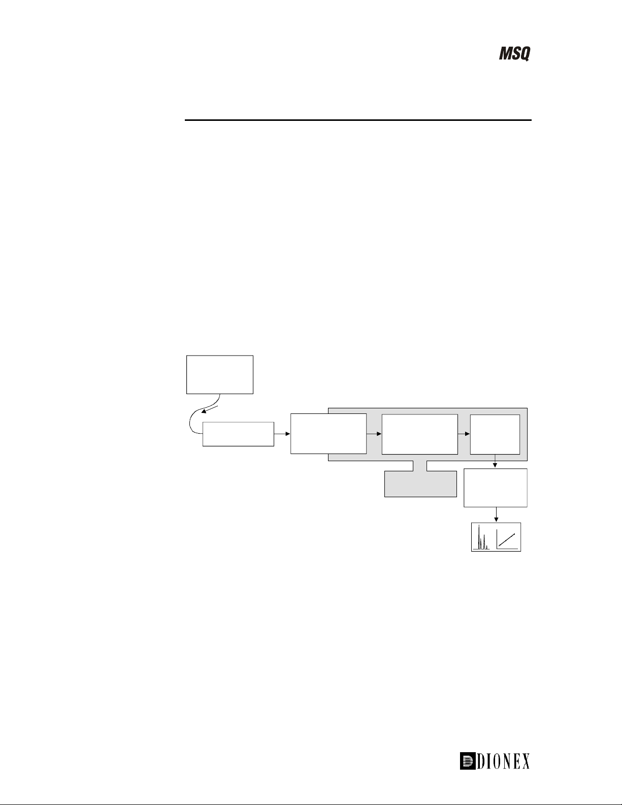
LC System

Sample

introduction

LC Column

Separation

Figure 1-1. The key components of the MSQ API LC detection system

Ion Source

Ionization &

transmission

Mass Analyzer

Sorting of ions

Turbomolecular

& rotary pumps

Molecular weight information

Structural information

Positive identification

Quantitative information

Detector

Detection

of ions

Data System

Windows NT

1-2 ___________________________ MSQ Hardware Manual ____________________________

Page 7

Introducing the MSQ

_______________________________________________________________________System Overview

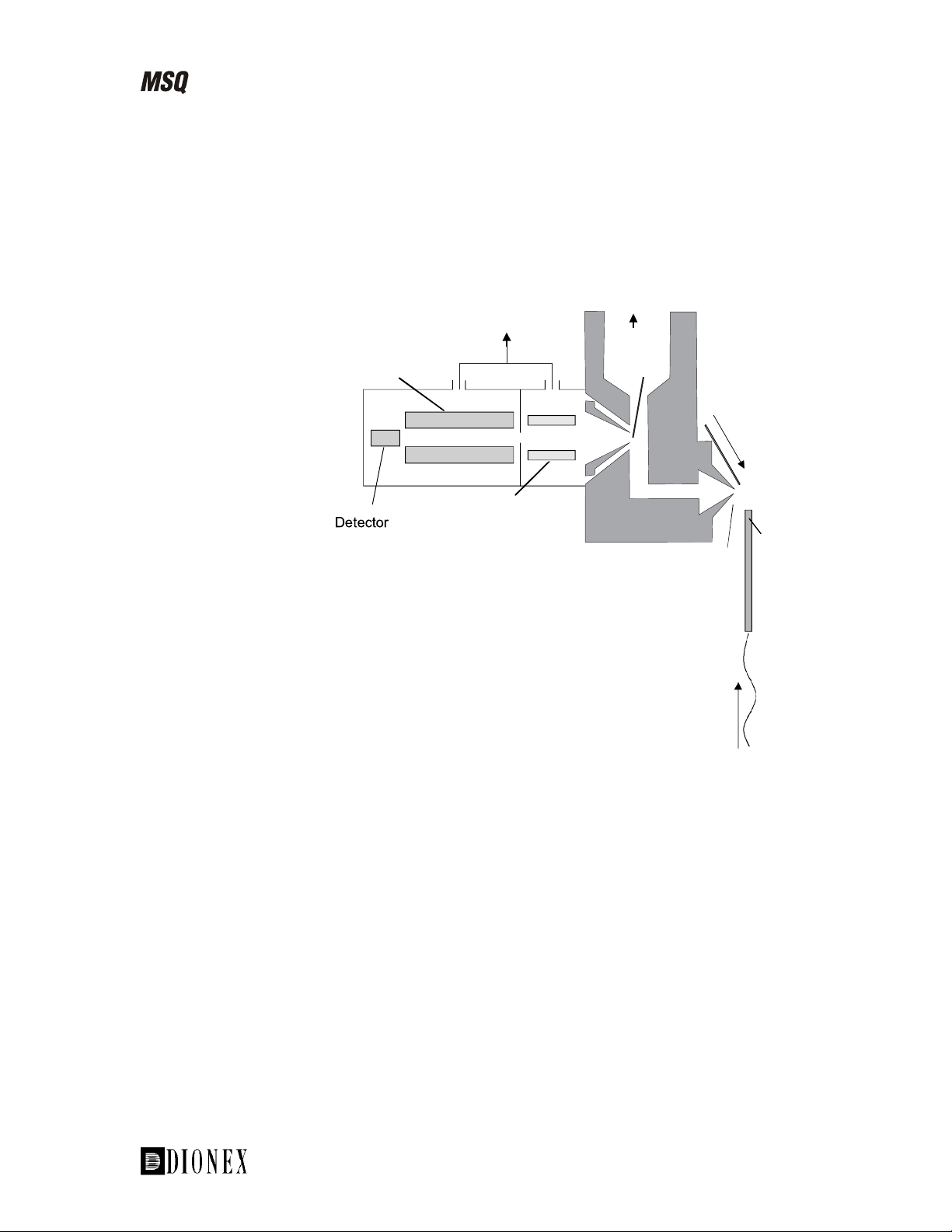
The main features of the MSQ MS detector are:

Dual ESI/APCI orthogonal probe •

• • Self-cleaning API-LC/MS interface

M-Path™ triple orthogonal source

Quadrupole mass analyzer

Split flow turbomolecular pump

Square quadrupole RF lens

Rotary pump

Exit cone

Entrance cone

From HPLC

Cone wash

Orthogonal sample introduction probe

Figure 1-2. Schematic diagram of the MSQ API inlet, analyzer, and

detector system

The LC eluent is ionized at the API probe and the resulting ions are focused into a square quadrupole RF lens. The quadrupole mass analyzer filters the ions before detection.

___________________________MSQ Hardware Manual ____________________________ 1-3

Page 8

Introducing the MSQ System Overview ________________________________________________________________________

What Is Mass Detection?

Mass detection is a very powerful analytical technique used in a number of fields, including:

Identification of unknown compounds •

• • Quantitation of known compounds

Determination of chemical structure

The basic function of an MS detector is to measure the mass-to-charge ratio of ions.

The unit of mass used is the Dalton (Da). One Dalton is equal to 1/12 of the mass of a single atom of carbon-12. This follows the accepted convention that an atom of carbon-12 has exactly 12 atomic mass units (amu). The MS detector does not directly measure molecular mass, but the mass-to-charge ratio of the ions. Electrical charge is a quantized property and so can exist only as an integer; that is, 1, 2, 3, and so on. The unit of charge used here (z) is that which is on an electron (negative) or a proton (positive). Therefore, the mass-to-charge ratio measured can be denoted by m/z. Most ions encountered in mass detection have just one charge. In this case, the massto-charge ratio is often spoken of as the “mass” of the ion.

1-4 ___________________________ MSQ Hardware Manual ____________________________

Page 9

Introducing the MSQ

_______________________________________________________________________System Overview

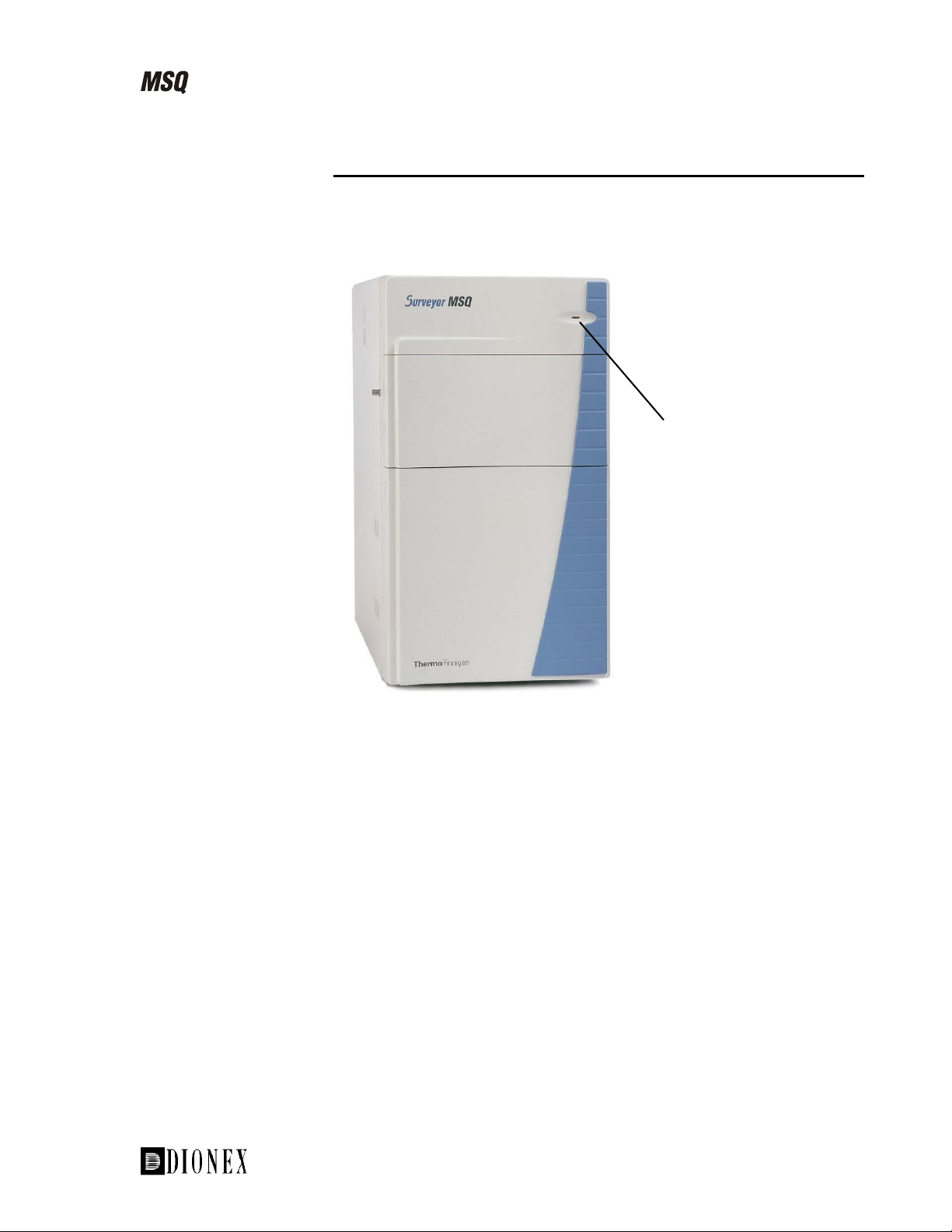
Exterior Features of the MSQ

This section highlights the exterior features of the MSQ. The parts labeled here may be referred to in later chapters of this manual or other manuals supplied with the MSQ.

Status light

Figure 1-3. Front view of the MSQ

Figure 1-3 shows the front view of the MSQ. The main feature is the status light.

___________________________MSQ Hardware Manual ____________________________ 1-5

Page 10

Introducing the MSQ System Overview ________________________________________________________________________

Table 1-1. Instrument status light

Instrument Status Light

Vented Red

Venting Red

Pumping down Flashing yellow

Under vacuum (above vacuum trip)

Under vacuum (ready for use)

Operate on (MSQ in use)

Source enclosure open Red

Red

Yellow

Green

The vacuum trip is the pressure below which it is safe to switch on the voltages in the source. When the instrument is functioning normally, the status light will go from flashing yellow to solid yellow and Operate can be switched On. If the pressure in the instrument rises above the operating pressure, the status light turns red to indicate that the pressure is above a safe level. See the chapter Shutting Down and Restarting the System for information on pumping down the MSQ.

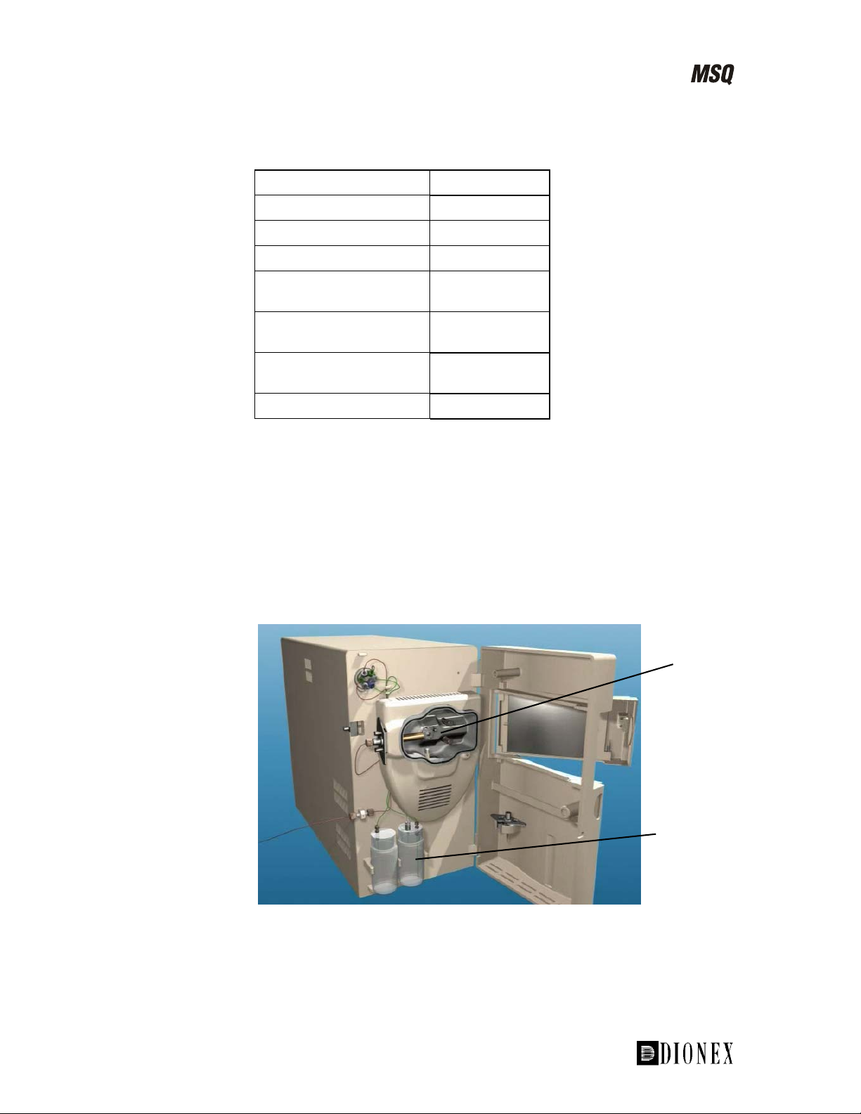
Figure 1-4 shows the MSQ with the doors open. The source enclosure and reference inlet are now visible.

Source enclosure

Figure 1-4. The MSQ with the doors open

1-6 ___________________________ MSQ Hardware Manual ____________________________

Reference inlet

Page 11

Introducing the MSQ

_______________________________________________________________________System Overview

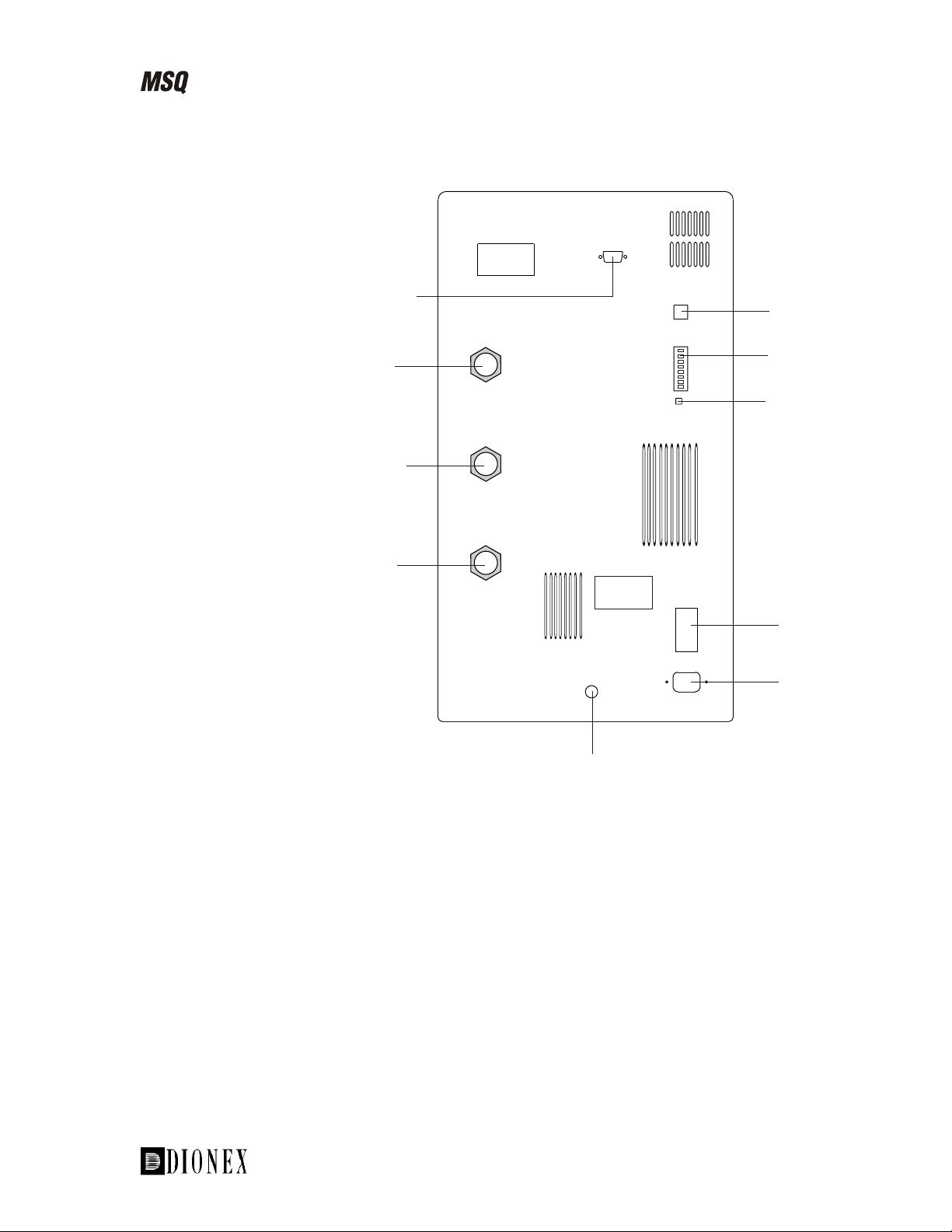
Figure 1-5 is a schematic of the rear view of the MSQ.

PUMP RELAY

Rotary pump power

To P C

Contact closure and analog inputs

To rotary pump

USB

SOURCE

USER I/O

EXHAUST

Exhaust from API source

BACKING

To rotary pump

Figure 1-5. Rear view of the MSQ

RESET

MODEL: RATING: 220-240v

GAS IN

6 BAR MAX

50/60 Hz 1000 VA

MAINS ON/OFF

Gas inlet for nebulizer and sheath gas

Reset communications

Power switch

MAINS IN

Power supply

___________________________MSQ Hardware Manual ____________________________ 1-7

Page 12

Introducing the MSQ The Source–An Introduction to API Techniques ________________________________________________

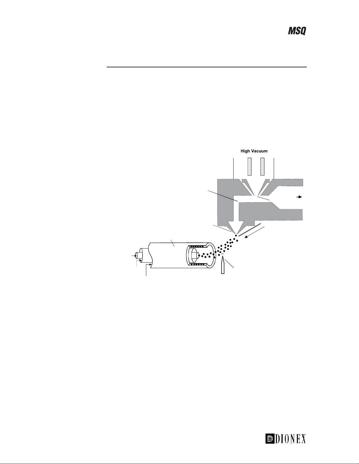
The Source–An Introduction to API Techniques

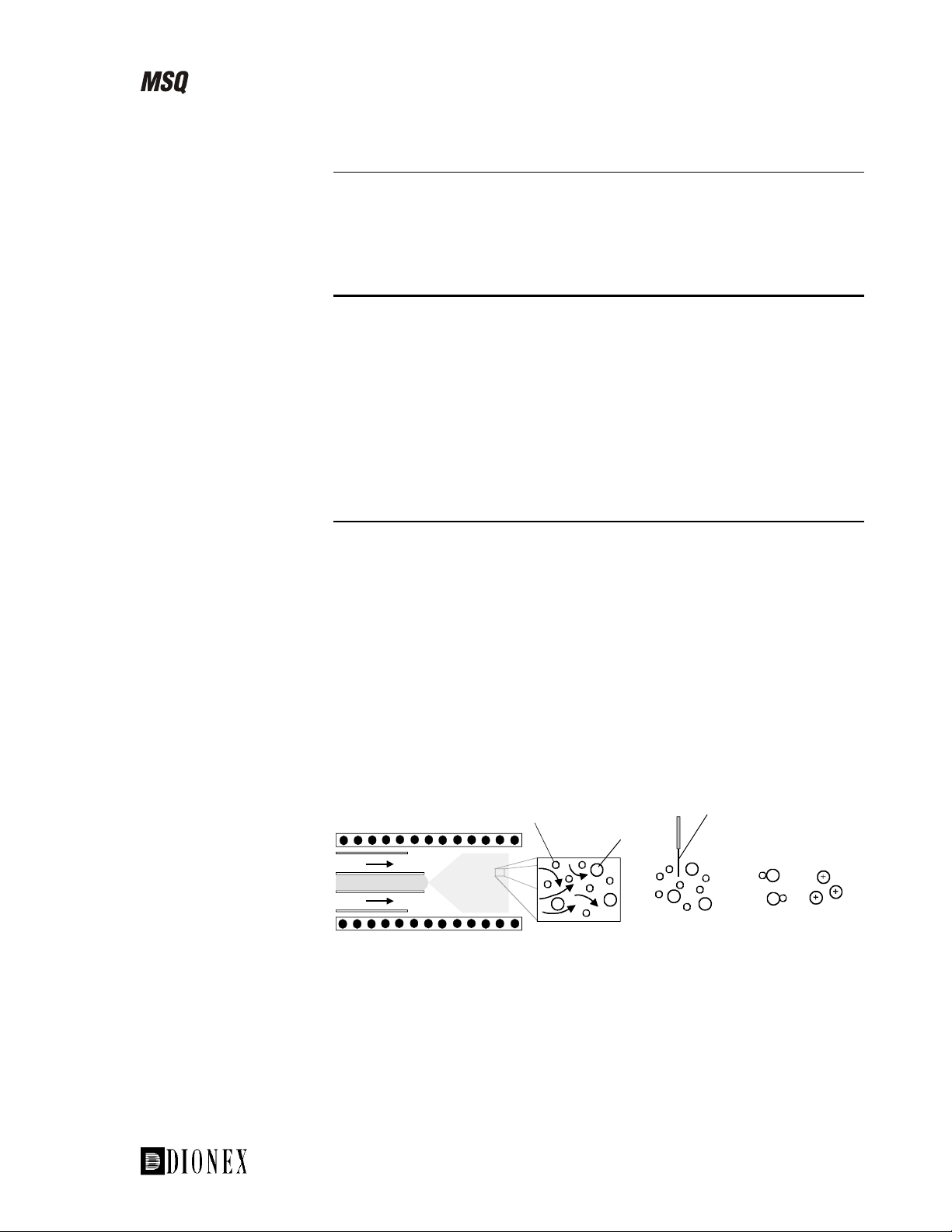
The source, or interface, performs four main functions:

Separates the analytes from the solvent and buffer systems used in LC •

• • Ionizes the analyte molecules

Allows efficient transfer of ions into the mass analyzer for detection

LC eluent enters the source through the orthogonal sample introduction probe. The primary objective of an orthogonal probe is to direct any involatile components present in the LC eluent, such as those from buffers, ion-pairing agents, or matrices, away from the entrance orifice. Under operating conditions, however, both the sample ions and the charged liquid droplets (containing any involatile components, if they are present) are deflected by the electric field towards the entrance orifice. This leads to a gradual buildup of involatiles and a concomitant loss in sensitivity with time. The self-cleaning source delivers a constant, low flow of solvent (the cone wash™) to the edge of the inlet orifice, helping to prevent a buildup of involatiles during an LC/MS run.

1-8 ___________________________ MSQ Hardware Manual ____________________________

Page 13

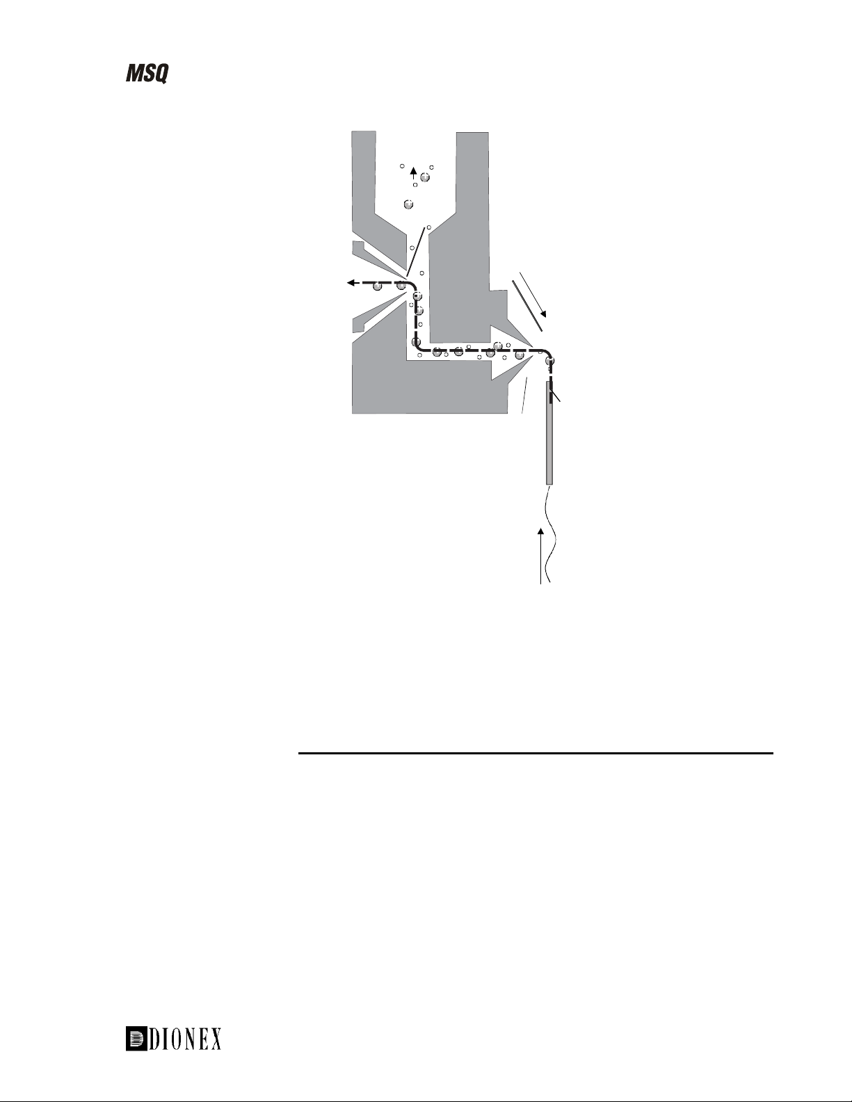
Introducing the MSQ

_______________________________________________ The Source–An Introduction to API Techniques

Rotary pump

Exit cone

To the mass analyzer

Entrance cone

From HPLC

Figure 1-7. Schematic of the MSQ source showing the cone wash

Cone wash

Orthogonal sample introduction probe

Two types of API are commonly encountered. These are Electrospray Ionization (ESI) and Atmospheric Pressure Chemical Ionization (APCI). The following sections discuss the mechanism of ion generation in each.

Electrospray

Electrospray Ionization (ESI) is regarded as a soft ionization technique providing a sensitive means of analyzing a wide range of polar molecules. Since the first combined ESI LC/MS results were announced in 1984, and its first application to protein analysis four years later, the technique has become an established analytical tool in separation science.

When applied to smaller molecules up to 1000 Daltons in molecular mass, electrospray ionization results in either a protonated, [M+H] 1-8) or deprotonated, [M-H]

, molecule. Choice of ionization mode is governed by the functional chemistry of the molecule under investigation. In ESI, fragmentation is generally not apparent; however, increased source voltages can induce fragmentation to provide structural information.

___________________________MSQ Hardware Manual ____________________________ 1-9

(see Figure

Page 14

Introducing the MSQ

The Source–An Introduction to API Techniques ________________________________________________

100

240

tBu

Chemical structure of salbutamol, (molecular weight 239)

60 80 100 120 140 160 180 200 220 240 260 280 300

241

Figure 1-8. Electrospray mass spectrum of salbutamol in positive ion

mode

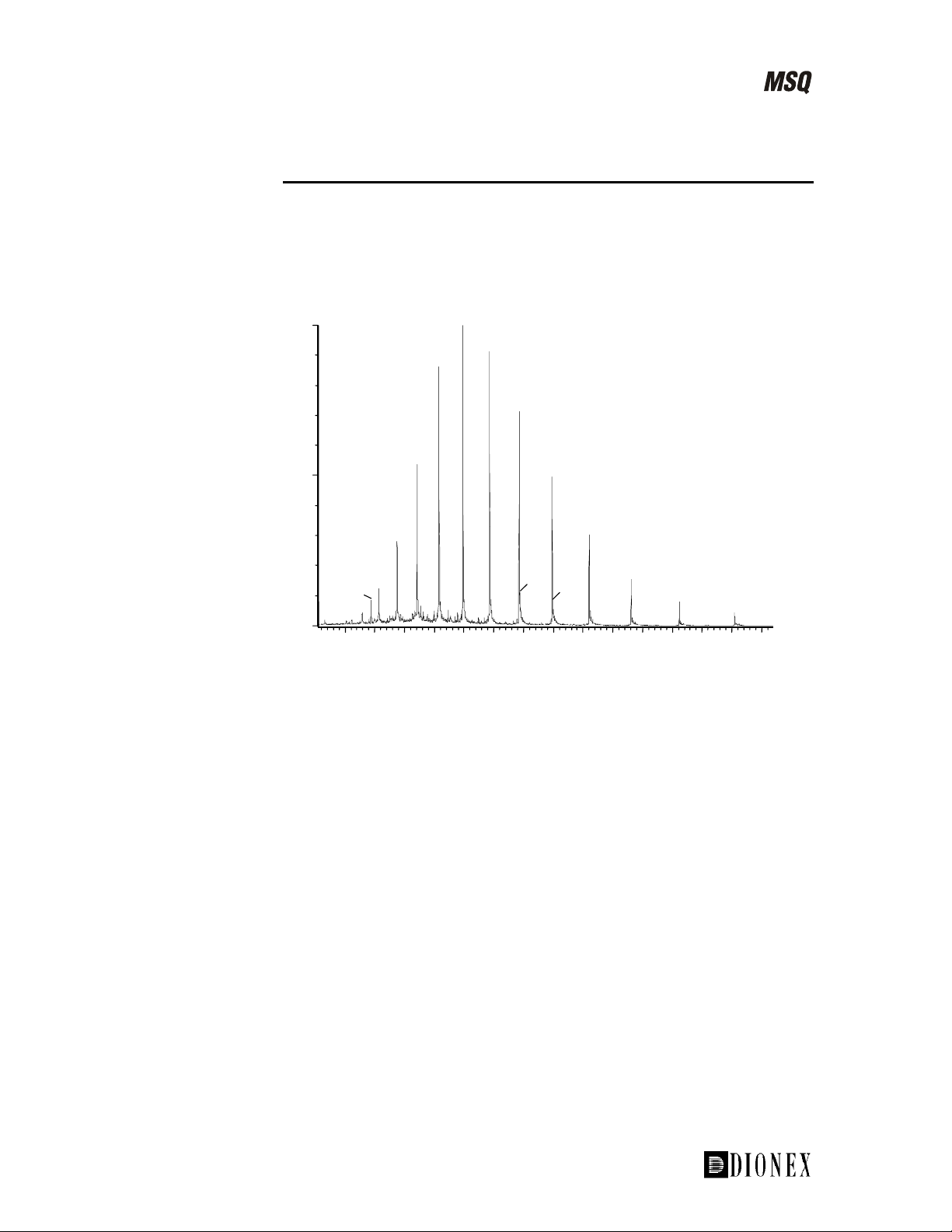
The base peak at m/z 240 (see Figure 1-8) corresponds to the protonated salbutamol molecule. It is notable that ESI results in a prominent base peak with minimal fragmentation, quite dissimilar from the results often achieved with GC/MS.

Mechanism of Ion Generation

Electrospray ionization operates by the process of emission of ions from a droplet into the gas phase, a process termed Ion Evaporation. A solvent is pumped through a stainless steel insert capillary that carries a high potential, typically 3 to 5 kV (see Figure 1-9). The strong electric field generated by this potential causes the solvent to be sprayed from the end of the insert capillary (hence, electrospray), producing highly charged droplets. As the solvent is removed by the desolvation process, the charge density on the surface of the droplets increases until the Rayleigh limit is exceeded; after this, a multitude of smaller droplets are formed by coulombic explosion. This process is repeated until charged sample ions remain. These ions are then available for sampling by the ion source.

Insert capillary +3-5 kV

Droplet containing ions

As the droplet evaporates, the electric field increases and ions move towards the surface

Figure 1-9. Positive ion electrospray mechanism

Ions evaporate from the surface

1-10 __________________________ MSQ Hardware Manual ____________________________

Page 15

Introducing the MSQ

_______________________________________________ The Source–An Introduction to API Techniques

Electrospray Ionization Using the MSQ Source

The sample, in solution, enters the source via a stainless steel insert capillary held at a voltage of 3 to 5 kV. The insert capillary is surrounded by a tube that directs a concentric flow of nitrogen nebulizing gas past the droplets of liquid forming at the probe tip. The action of the nebulizing gas, high voltage, and heated probe produces an aerosol of liquid droplets containing ions of the sample and solvent. The ion evaporation process is assisted by a second concentric flow of heated nitrogen gas. This is the sheath gas. This highly efficient evaporation process close to the entrance cone enables the routine use of high LC flow rates (up to 2.0 mL/min) in ESI mode.

The newly formed ions then enter the focusing region through the entrance cone. This is due to the following:

The high electric field. The insert capillary is at 3 to 5 kV with respect

•

to the rest of the source, which is typically at 20 to 30 V.

• The gas flow into the focusing region.

Ions then exit the focusing region and pass into the RF lens. The RF lens (square quadrupole) helps to focus the ions before they enter the mass analyzer region.

Region

Intermediate

Pressure

Region

Exit cone

Entrance cone

Probe

Insert capillary

LC eluent

Nebulizing gas, N

Sheath gas, N

Insert

Cone Wash

Atmospheric

Pressure

Region

Figure 1-10. Schematic of the ESI source on the MSQ, showing the

principal components and pressure regions

Rotary pump

___________________________MSQ Hardware Manual ___________________________ 1-11

Page 16

Introducing the MSQ The Source–An Introduction to API Techniques ________________________________________________

Spectral Characteristics

Polar compounds of low molecular weight (<1000 amu) typically form singly charged ions by the loss or gain of a proton. Basic compounds (for example, amines) can form a protonated molecule [M+H] analyzed in positive ion mode to give a peak at m/z M+1. Acidic compounds (for example, sulphonic acids) can form a deprotonated molecule [M-H]

, which can be analyzed in negative ion mode to give a peak at m/z M-1. As electrospray is a very soft ionization technique, there is usually little or no fragmentation and the spectrum contains only the protonated or deprotonated molecule.

Some compounds are susceptible to adduct formation if ionization takes place in the presence of contamination or additives such as ammonium or sodium ions. The spectra will show other ions in addition to, or instead of, the quasi-molecular ion. Common adducts are ammonium ions NH [M+18]

100

, sodium ions Na+ [M+23]+, and potassium ions K+ [M+39]+.

, which can be

[M+H]

322

100

103

60 80 100 120 140 160 180 200 220 240 260 280 300 320 340 360

141

145

181

187

241

244

261

279

282

[M+Na]

344

363

m/z

Figure 1-11. Electrospray spectrum showing a sodium adduct

The singly charged ions arising from samples of relatively low molecular masses can be interpreted directly, as they represent the protonated or deprotonated molecule. Electrospray, however, can produce multiply charged ions for analytes that contain multiple basic or acidic sites, such as proteins and peptides. As an MS detector measures mass-to-charge ratio (m/z), these ions appear at a m/z value given by the mass of their protonated molecule divided by the number of charges:

nHM

 



 



Where, M = actual mass, n = number of charges, and H = mass of a proton.

Electrospray allows molecules with molecular weights greater than the mass range of the MS detector to be analyzed. This is a unique feature of electrospray.

1-12 __________________________ MSQ Hardware Manual ____________________________

Page 17

Introducing the MSQ

_______________________________________________ The Source–An Introduction to API Techniques

Flow Rate

The electrospray source can be used with flow rates from 5.0 µL/min to

2.0 mL/min.

Atmospheric Pressure Chemical Ionization

Atmospheric Pressure Chemical Ionization (APCI) is also a very soft ionization technique and has many similarities to electrospray ionization. Ionization takes place at atmospheric pressure and the ions are extracted into the MS detector in the same way as in electrospray.

Similarly, as observed in ESI, [M+H] providing molecular weight information. Fragmentation can be induced in the source by increasing the source voltage to give structural information.

Mechanism of Ion Generation

and [M-H]- ions are usually formed

In APCI, the liquid elutes from an insert capillary, surrounded by a coaxial flow of nitrogen nebulizing gas into a heated region. The combination of nebulizing gas and heat form an aerosol that evaporates quickly to yield desolvated neutral molecules (see Figure 1-12).

At the end of the probe is a corona pin held at a high potential (typically 2.0 to 3.5 kV). This produces a high-field corona discharge that causes solvent molecules eluting into the source to be ionized. In the atmospheric pressure region surrounding the corona pin, a series of reactions occur that give rise to charged reagent ions. Any sample molecules, which elute and pass through this region of reagent ions, can be ionized by the transfer of a proton to form [M+H]

or [M-H]-. This is a form of chemical ionization; hence the

name of the technique, Atmospheric Pressure Chemical Ionization.

Heated nebuliser

Liquid

Solvent molecules

An aerosol is formed

Sample molecules

Solvent and

sample molecules

are desolvated

Corona pin

Collisions and

proton transfer

Solvent molecules

are ionized

Sample

[M+H]

ions formed

Figure 1-12. Positive ion APCI mechanism

___________________________MSQ Hardware Manual ___________________________ 1-13

Page 18

Introducing the MSQ The Source–An Introduction to API Techniques ________________________________________________

APCI Using the MSQ Source

The sample is carried to a spray region via a stainless steel insert capillary. The action of both the nebulizing gas and the heated probe leads to the formation of an aerosol. The desolvation process is assisted by a second concentric flow of nitrogen gas, the sheath gas.

In contrast to electrospray, APCI is a gas phase ionization technique. Ionization occurs as the aerosol leaves the heated nebulizer region. A corona pin, mounted between the heated region and the entrance cone, ionizes the sample molecules with a discharge voltage of approximately 3.0 to 3.5 kV in positive ion mode and 2.0 to 3.0 kV in negative ion mode.

Region

Intermediate

Pressure

Region

Exit cone

Rotary pump

Entrance cone

Pressure

Region

Cone Wash

LC eluent

Nebulizing gas, N

Sheath gas, N

Probe

Atmospheric

Corona pin

Figure 1-13. Schematic of the APCI source on the MSQ, showing the

principal components and pressure regions

The newly formed ions then enter the focusing region through the entrance orifice and pass into the RF lens region. The RF lens (square quadrupole) helps to focus the ions before they enter the mass analyzer region.

1-14 __________________________ MSQ Hardware Manual ____________________________

Page 19

Introducing the MSQ

_______________________________________________ The Source–An Introduction to API Techniques

Spectral Characteristics

Like electrospray, APCI is a soft ionization technique and forms singly charged ions–either the protonated, [M+H]

, or deprotonated, [M-H]-, molecule–depending on the selected ionization mode. Unlike electrospray, however, APCI does not produce multiply charged ions and so is unsuitable for the analysis of high molecular weight compounds such as proteins or peptides.

Although a high temperature is applied to the probe, most of the heat is used in evaporating the solvent, so the thermal effect on the sample is minimal. In certain circumstances (for example, with very thermally labile (unstable) compounds), the heated probe may cause some thermal fragmentation.

Flow Rate

Flow rates of 0.2 to 2.0 mL/min can be used with APCI.

___________________________MSQ Hardware Manual ___________________________ 1-15

Page 20

Introducing the MSQ The Source–An Introduction to API Techniques ________________________________________________

Source Fragmentation

Both electrospray and APCI are regarded as soft ionization techniques. Ionization generally results in spectra dominated by either the protonated molecule [M+H] (negative ion mode), depending on whether positive or negative ionization mode has been selected. Choice of ionization mode is governed by the functional chemistry of the molecule under investigation.

Source fragmentation can be induced to give additional information on a compound, such as diagnostic fragment ions for structural determination or an increased response on a particular confirmatory ion for peak targeting.

Formation of Diagnostic Fragment Ions

The MSQ allows the simultaneous acquisition of MS data at a number of different source voltages. For example, the MSQ can be programmed to acquire data at source voltages of 20, 40, and 60 V on an alternating scan basis within a single acquisition. The benefits of setting up acquisitions in this way are:

(positive ion mode) or deprotonated molecule [M-H]-

The optimum source voltage for a particular ion can be determined in

•

one acquisition for compounds where sample volume is at a premium.

• The intensity of fragment ions can be maximized to gain structural

information.

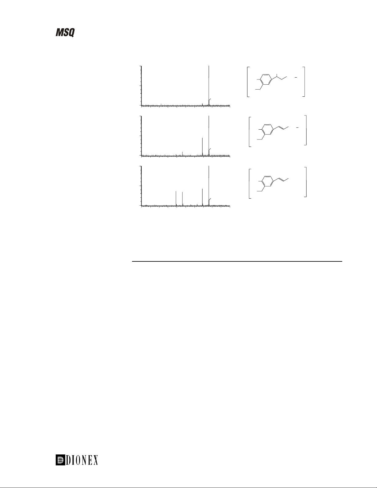
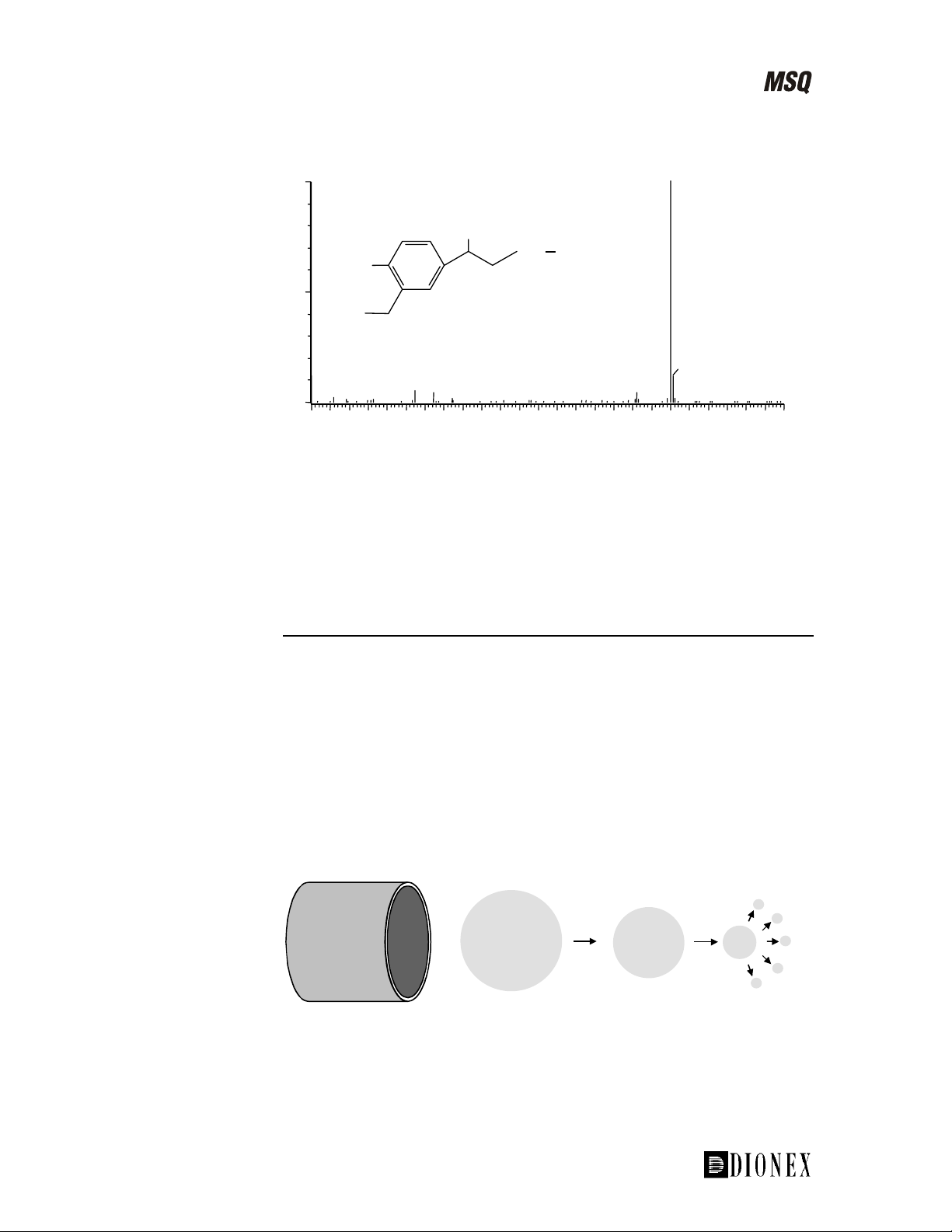
Fragmentation at increased source voltages is useful for most compounds. For example, using source fragmentation of salbutamol in electrospray ionization, a number of confirmatory fragment ions can be generated and their intensity maximized (see Figure 1-14).

The mechanism for the formation of the fragment ions is characteristic for not only salbutamol, but also for related β-agonists such as clenbuterol,

terbutaline, and metaproterenol. It involves loss of water (-18 amu; resulting in the fragment ion at m/z 222 (middle trace)) and an additional loss of the tert-butyl group (-56 amu; resulting in the fragment at m/z 166 (lower trace)).

Note. The MSQ uses the term “cone voltage” to represent source voltage.

1-16 __________________________ MSQ Hardware Manual ____________________________

Page 21

Introducing the MSQ

_______________________________________________ The Source–An Introduction to API Techniques

100

Source voltage 10V

50 75 100 125 150 175 200 225 250 275 300

100

Source voltage 25V

50 75 100 125 150 175 200 225 250 275 300

100

Source voltage 35V

50 75 100 125 150 175 200 225 250 275 300

148

166

240

241

240

222

241

240

222

241

m/z

Protonated molecule at m/z 240

tBu

Fragment ion at m/z 222

tBu

Fragment ion at m/z 166

[M+H]

[M+H]+-H2O

[M+H]+-H2O-tB

Figure 1-14. Source fragmentation of salbutamol in electrospray

ionization

Optimum Response for Confirmatory Ions

When acquiring fragment ions for confirmation purposes, the applied source voltage per compound would require some optimization to maximize the intensity of these ions. It is generally observed that small changes to the source voltage result in only small intensity changes; thus, fine-tuning of this voltage is usually not critical (typically +/- 5 V is adequate).

___________________________MSQ Hardware Manual ___________________________ 1-17

Page 22

Introducing the MSQ The Source–An Introduction to API Techniques ________________________________________________

Cone Voltage Ramping

Source voltage ramping can be used in Full Scan operation (see page 1-32) in electrospray when the compound of interest forms multiply charged ions. A spectrum similar to that in Figure 1-15 will be produced, showing the multiply charged envelope.

771

808

848

893

942

944

998

999

1060

1131

1212

1305

m/z

100

738

707

694

700 800 900 1000 1100 1200 1300

Figure 1-15. Electrospray spectrum of horse heart myoglobin

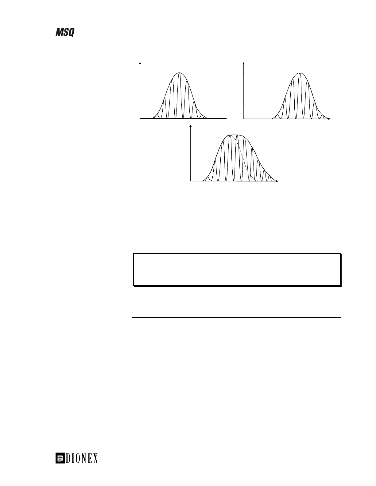
This envelope is represented in diagrammatic form in Figure 1-16. The first diagram shows the envelope at a source voltage of 30 V. Next, the envelope is shown at 60 V. There is no ramping applied here. The envelope has the same shape but has moved to a higher m/z value. This is due to the charge stripping that occurs at high source voltages, which lowers the charge state and produces an apparent higher mass distribution. If the source voltage is ramped between 30 and 60 V, the charge distribution envelope is extended and it resembles the lower diagram.

1-18 __________________________ MSQ Hardware Manual ____________________________

Page 23

Introducing the MSQ

_______________________________________________ The Source–An Introduction to API Techniques

Intensity

Without s ource voltage ramping

Source voltage 30V

Increasing number of charges

Intensity

Decreasing

number o

charges

With source voltage ramping 30-60V

m/z

Intensity

Without s ource voltage ramping

Source voltage 60V

m/z

Figure 1-16. Cone voltage ramping

Cone voltage ramping is often used for proteins and peptides during:

Calibration (to extend the calibration range) •

• Analysis (to increase the number of charge states leading to greater

accuracy of molecular weight determination)

m/z

Note. Cone voltage ramping will not perform source fragmentation because the same cone voltage corresponds to the same m/z value each time.

Polarity Switching

Switching between positive and negative ionization modes in a single analytical run is supported by the MSQ. Rapid polarity switching is a technique that is applied to several important areas of MS analysis; for example:

Quantitation of different chemistries within the same run. In drug

•

metabolism studies, certain compounds preferentially ionize in positive ion mode because they may contain a primary amino group. Other metabolites, such as glucuronide metabolites, are likely to lose a proton and respond in the negative ion mode.

• Rapid screening of unknown analytes; for example, in combinatorial

chemistry. If the compound has a carboxylic acid group that is sterically unhindered, it is likely that the compound will lose a proton in negative ion mode and not respond in positive ion mode.

___________________________MSQ Hardware Manual ___________________________ 1-19

Page 24

Introducing the MSQ

The Source–An Introduction to API Techniques ________________________________________________

Application of API Techniques

Both electrospray and APCI are ideal for online liquid chromatography detection, providing an additional dimension of information. With many compounds, it is possible to analyze them by both APCI and electrospray. It may be difficult to decide which is the more appropriate technique, especially when the compounds of interest lack polar functionalities.

Points to note:

Electrospray is one of the softest ionization methods available, whereas

•

APCI, although also a soft ionization technique, may not be suitable for some very thermally labile compounds as there may be thermal fragmentation (see Figure 1-17).

214

231

PCI mass spectrum,

source voltage 25V.

Electrospray mass spectrum, source voltage 25V.

100

130 140 150 160 170 180 190 200 210 220 230 240

100

130 140 150 160 170 180 190 200 210 220 230 240

156

173

Figure 1-17. Thermal fragmentation of the herbicide asulam in APCI

APCI does not yield multiply charged ions like electrospray, and so is

•

unsuitable for the analysis of high molecular weight compounds such as proteins.

m/z

• Both APCI and electrospray generally provide data from which it is

simple to infer molecular weight values. In many cases, with the correct conditions, only one major peak is observed in the spectrum: either the protonated molecule [M+H] ion) or deprotonated molecule [M-H]

(-ve ion). However, some

(+ve

compounds are more susceptible to fragmentation than others, so different degrees of fragmentation may be seen from compound to compound. When determining molecular weights, always take account of possible adduct ions. Common adducts are [M+18]

(ammonium adducts seen in the presence of buffers such as ammonium acetate), [M+23]+ Na+ (sodium adducts), and [M+39]+ K+ (potassium adducts).

1-20 __________________________ MSQ Hardware Manual ____________________________

Page 25

Introducing the MSQ

_______________________________________________ The Source–An Introduction to API Techniques

Source fragmentation is used in both APCI and electrospray to give

•

structural information. In general, increasing the voltage applied to the source block (the cone voltage) yields increasing amounts of fragmentation, depending on the nature of the compound. The optimum source voltage required to give the maximum intensity of the protonated or deprotonated molecule is compound-dependent, as is the source voltage required for fragmentation. The energies involved in source fragmentation are low, so usually only weaker bonds such as C-N and C-O are broken.

Since there are many similarities between electrospray and APCI, there are many applications common to both.

Compounds suitable for analysis by electrospray are polar and of molecular weight less than 100,000 amu. The higher molecular weight compounds, such as proteins, can produce multiply charged ions. As it is the mass-tocharge ratio (m/z) that is measured by the MS detector, these can often be seen at lower masses. For example, if the molecular weight is 10,000, a doubly charged ion (2+ in +ve ion) would be seen at m/z 5001, 10+ at m/z 1001, etc.

Typical electrospray applications are: peptides, proteins, oligonucleotides, sugars, drugs, steroids, and pesticides.

Compounds suitable for analysis by APCI are generally polar (although less polar than electrospray) and of molecular weight <1000 amu.

Typical APCI applications are: pesticides, drugs, azo dyes, and steroids.

A summary comparing electrospray and APCI is shown in Table 1-2.

___________________________MSQ Hardware Manual ___________________________ 1-21

Page 26

Introducing the MSQ The Source–An Introduction to API Techniques ________________________________________________

Table 1-2. Comparison of ESI and APCI

LC/MS technique Electrospray (ESI) Atmospheric Pressure Chemical

Ionization (APCI)

Compound polarity Polar Polar, some non-polar

Examples Drugs, proteins, biopolymers,

oligonucleotides, steroids, and pesticides

Pesticides, azo dyes, drugs, metabolites, agrochemicals, and steroids

Sensitivity fg to pg (compound-dependent) fg to pg (compound-dependent)

Type of spectra [M+H]+ for +ve ion mode, [M-H]- for

-ve ion mode, fragmentation via source voltage

[M+H]

for +ve ion mode, [M-H]- for

-ve ion mode, fragmentation via source voltage

Flow rates 2.0 µL/min to 2.0 mL/min 0.2 to 2.0 mL/min

LC columns Capillary to 4.6-mm ID columns 2.1- to 4.6-mm ID columns

Mobile phases H2O, CH3CN, CH3OH are most

frequently used.

H2O, CH3CN, CH3OH are most frequently used. Non-polar solvents can be used.

Typical mass range <100,000 <1000

1-22 __________________________ MSQ Hardware Manual ____________________________

Page 27

Introducing the MSQ

______________________________________________________The Self-Cleaning Source: Cone Wash

The Self-Cleaning Source: Cone Wash

This section introduces the cone wash. Information on how and when to use it is provided in the chapter LC/MS and the Cone Wash.

Introduction

The API source on the MSQ includes a self-cleaning solvent delivery system (the cone wash). This makes the source extremely robust and productive and greatly increases the number of samples that can be analyzed before maintenance is required.

The orthogonal API probe serves to direct the LC eluent away from the inlet orifice. However, under typical LC/MS conditions, both the ions and the charged liquid droplets (containing involatile components) are deflected by the electric field towards the inlet orifice. This effect leads to a gradual buildup of involatile components and an associated loss in sensitivity with time.

The self-cleaning API source delivers a constant, low flow of solvent to the edge of the inlet orifice (see Figure 1-18). This prevents the buildup of involatile components during LC/MS analysis with typical chromatographic buffers (for example, phosphates and ion-pairing agents). This greatly improves the quantitation precision of analysis without the need to compromise the LC method, and more importantly, dramatically extends the length of time possible for analysis.

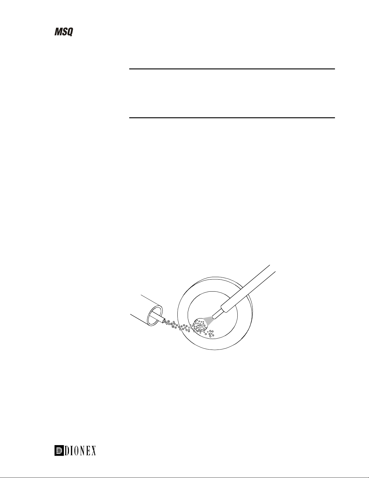
Figure 1-18. Dispersion of involatile components from the inlet orifice

___________________________MSQ Hardware Manual ___________________________ 1-23

Page 28

Introducing the MSQ The Self-Cleaning Source: Cone Wash _______________________________________________________

Functional Description

As shown in Figure 1-18, the cone wash nozzle consists of a stainless steel capillary, which is fed to the edge of the inlet orifice of the entrance cone. The capillary is attached to PEEK tubing, internal to the instrument, which when connected to an LC pump delivers the solvent (typically HPLC-grade water or organic solvents such as methanol) at a controlled flow rate.

Note. It is necessary to use the cone wash only for compounds in dirty matrices or when involatile buffers are used. Choose the cone wash solvent to give the most effective solubility for the expected contaminants.

1-24 __________________________ MSQ Hardware Manual ____________________________

Page 29

Introducing the MSQ

______________________________________________________________ The Reference Inlet System

The Reference Inlet System

This section introduces the reference inlet system. Information on how to set up the system is provided in the chapter Reference Inlet System.

Introduction

The recommended way to introduce a sample for tuning and mass calibration in electrospray is to use the reference inlet system.

Functional Description

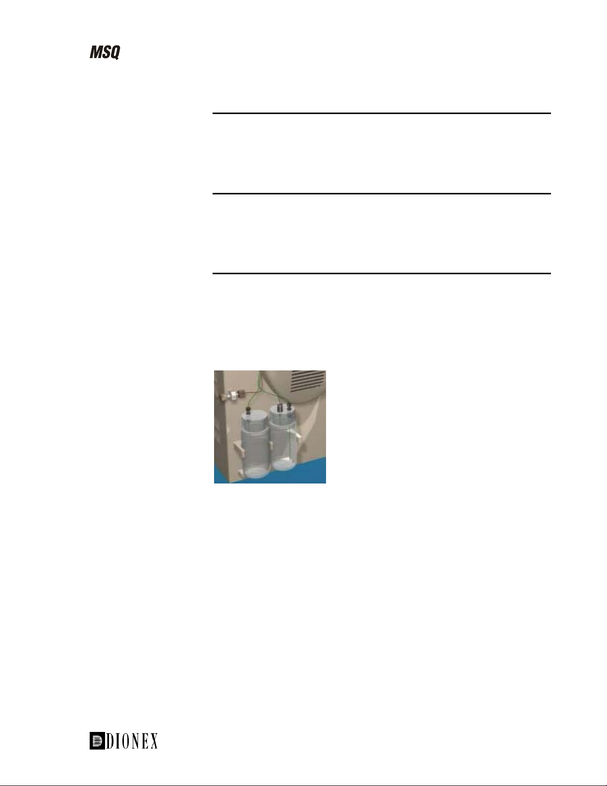
As shown in Figure 1-20, the reference inlet system consists of a pressurized reservoir containing the reference sample and a PEEK delivery tube. One end of the PEEK delivery tube is inserted into the reference inlet reservoir, while the other end is attached to the switching valve. When the pressure in the reservoir is increased, the sample is forced through the PEEK tube and infused directly into the 100 µL sample loop.

Figure 1-20. The reference inlet system

___________________________MSQ Hardware Manual ___________________________ 1-25

Page 30

Introducing the MSQ The Mass Analyzer and Detector____________________________________________________________

The Mass Analyzer and Detector

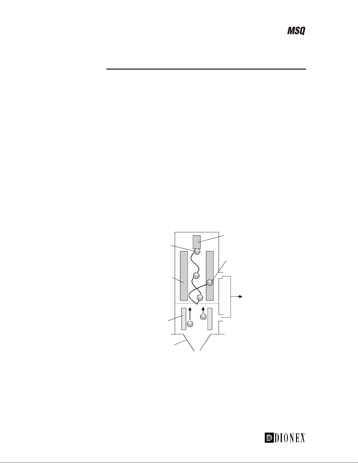
The mass analysis and detection system comprises two main components:

A quadrupole mass analyzer •

• A detector whose main component is a channeltron electron multiplier

The square quadrupole RF lens helps to focus the ions before they are filtered, according to their mass-to-charge ratio in the mass analyzer.

The analyzer in the MSQ is a quadrupole. This is one of the most widely used types of analyzer and can be easily interfaced to various inlet systems. By applying carefully controlled voltages to the four rods in the quadrupole, only ions of a specific mass-to-charge ratio are allowed to pass through at any one time.

The ions then reach the detector, whose main component is a channeltron electron multiplier. In positive ion mode, the ions exit the analyzer and strike a conversion dynode, which results in the emission of electrons. The electrons are accelerated towards the channeltron electron multiplier, which then creates an electron cascade. The current is then converted and amplified into a voltage signal that is analyzed and processed by the MSQ’s on-board data acquisition system. The resultant peak information is sent to the data system.

Ion successfully transmitted

by the mass analyzer

Quadrupole

mass analyzer

Square quadrupole RF lens

Source exit cone

Figure 1-21. Schematic of the MSQ analyzer and detector

Detector

Ion trajectory incorrect

for transmission trough

the mass analyzer

Split flow turbomolecular pump

1-26 __________________________ MSQ Hardware Manual ____________________________

Page 31

Introducing the MSQ

____________________________________________________________________ The Vacuum System

The Vacuum System

The main challenge in interfacing MS with LC is the introduction of a liquid mobile phase at flow rates of up to 2.0 mL/min into a system that operates under vacuum. The transition between atmospheric pressure and high vacuum is achieved by using several different stages of pressure controlled by the vacuum system. This arrangement effectively removes the mobile phase, leaving the analytes to travel as ions through the mass analyzer.

It is important to remember that an MS detector must be under high vacuum in order to operate. In the case of the MSQ system, not all of the MS detector is under high vacuum. The ion source is held at atmospheric pressure, while the region between the entrance and exit cones is held at an intermediate pressure to step down to the high vacuum region in the mass analyzer and detector. The intermediate pressure region is pumped by one rotary pump. The high vacuum in the mass analyzer and detector region is achieved by using a split-flow turbomolecular pump. All the pumps are controlled by the data system.

___________________________MSQ Hardware Manual ___________________________ 1-27

Page 32

Introducing the MSQ The Data System ________________________________________________________________________

The Data System

The data system has complete control of the MSQ system and runs on a Microsoft® Windows platform.

Software

Xcalibur™ software controls the MSQ MS detector. When Xcalibur is run, the Home page is displayed (see Figure 1-22). Xcalibur also runs the MSQ server (see Figure 1-23).

The Home Page

The Home page opens to show a ‘road map’ view of the data system.

Figure 1-22. The Xcalibur Home page “road map” view

1-28 __________________________ MSQ Hardware Manual ____________________________

Page 33

Introducing the MSQ

_______________________________________________________________________The Data System

The icons shown on the road map provide an easy way to access all the major modules of the data system. These modules are:

Instrument Setup •

Use Instrument Setup to configure the MSQ and all your LC equipment for acquisition. This information is saved as an instrument method.

•

Processing Setup

Use Processing Setup to specify all parameters for processing, reporting, and manipulation of acquired data. This information is saved as a processing method.

•

Sequence Setup

Use Sequence Setup to enter the details of the samples to be examined, including instrument and processing methods, and to control the acquisition of data.

•

Qual Browser

Use Qual Browser to examine acquired data, both chromatograms and spectra, in order to obtain more information about the compounds in the sample.

•

Quan Browser

Use Quan Browser to examine acquired data in order to obtain an accurate determination of the amounts of individual components present in a sample.

•

Library Browser

Use Library Browser to create your own libraries of spectra and to perform searches of those libraries.

The Server

The server is displayed as an icon on the Windows taskbar. In Figure 1-23, it is shown just to the left of the time display. The light will be red, yellow, or green, depending on the status of the system.

Figure 1-23. The taskbar showing the Xcalibur Home page and server

The server is shown as one light. When the light is green, the MSQ is under vacuum with Operate On and the API gas flowing. When the MSQ is pumping down, the light is yellow and flashing.

Use the server to tune and calibrate the MSQ and to pump or vent the system.

___________________________MSQ Hardware Manual ___________________________ 1-29

Page 34

Introducing the MSQ The Data System ________________________________________________________________________

Right-click on the server to display a menu:

Choose Instrument Tune and Calibration to display the Instrument

•

Tuning and Calibration Wizard.

Figure 1-24. The MSQ Instrument Tuning and Calibration Wizard

Choose Tune to display the Tune page. •

• • Choose Pump to pump down the MSQ or Vent to vent the MSQ.

Choose Exit to close the server. If Xcalibur is still running, this will not be allowed and an error message will be displayed.

Raw Data

Xcalibur acquires data in a “raw” file. Raw data can be viewed as chromatograms and mass spectra (see Figure 1-25).

The term mass spectrum refers to a plot of mass-to-charge ratio (m/z) versus relative abundance information. The mass spectrum at a particular time in an analytical run will reveal a “snapshot” of the data at that time.

The chromatogram is a plot of relative abundance versus time. Xcalibur produces the following types of chromatograms: total ion current (TIC) chromatogram, base peak chromatogram, mass range chromatogram, and analog UV chromatogram.

1-30 __________________________ MSQ Hardware Manual ____________________________

Page 35

Introducing the MSQ

_______________________________________________________________________The Data System

RT: 1.09 - 6.11

10 0

1. 2 4 1. 5 5 2 . 2 5

Relat ive Abundanc e

1. 5 2.0 2.5 3.0 3.5 4.0 4.5 5.0 5.5 6.0

carb mix pmix03#102 RT: 2.66 AV: 1 SB: 38 1.42-2.07, 2.87-3.15 NL: 1.02E5

T: + c ESI Ful l ms [ 150.00-500.00]

100

Relative Abundance

181.5 387.0

150 200 250 300 350 400 450 500

2.35

229.4

2.66

240.3

2.82

3.28

281.2

3.59

Time (min)

282.5

3.72

3.87

346.8 403.2

m/z

4.75

5.174.18 5.32

454.1

5.42

459.1

NL:

2.49E5 TIC carb

mix pmix03

461.0256.2

482.1

Figure 1-25. A mass spectrum taken at retention time 2.66 minutes

(lower trace) from a TIC chromatogram (upper trace)

Raw Data Types

The data can be collected and stored by the data system in two different ways: Full Scan and Selected Ion Monitoring (SIM). The main difference between these two modes is:

In Full Scan mode, data is collected across the whole scan range. •

• In SIM mode, data is acquired only at specific mass-to-charge ratios.

___________________________MSQ Hardware Manual ___________________________ 1-31

Page 36

Introducing the MSQ The Data System ________________________________________________________________________

Full Scan Mode

There are three different types of Full Scan acquisition. These are:

Centroid •

• • Profile

MCA (Multi Channel Analysis)

In all full scan acquisitions, raw data is collected over the whole scan range defined by the start and end mass.

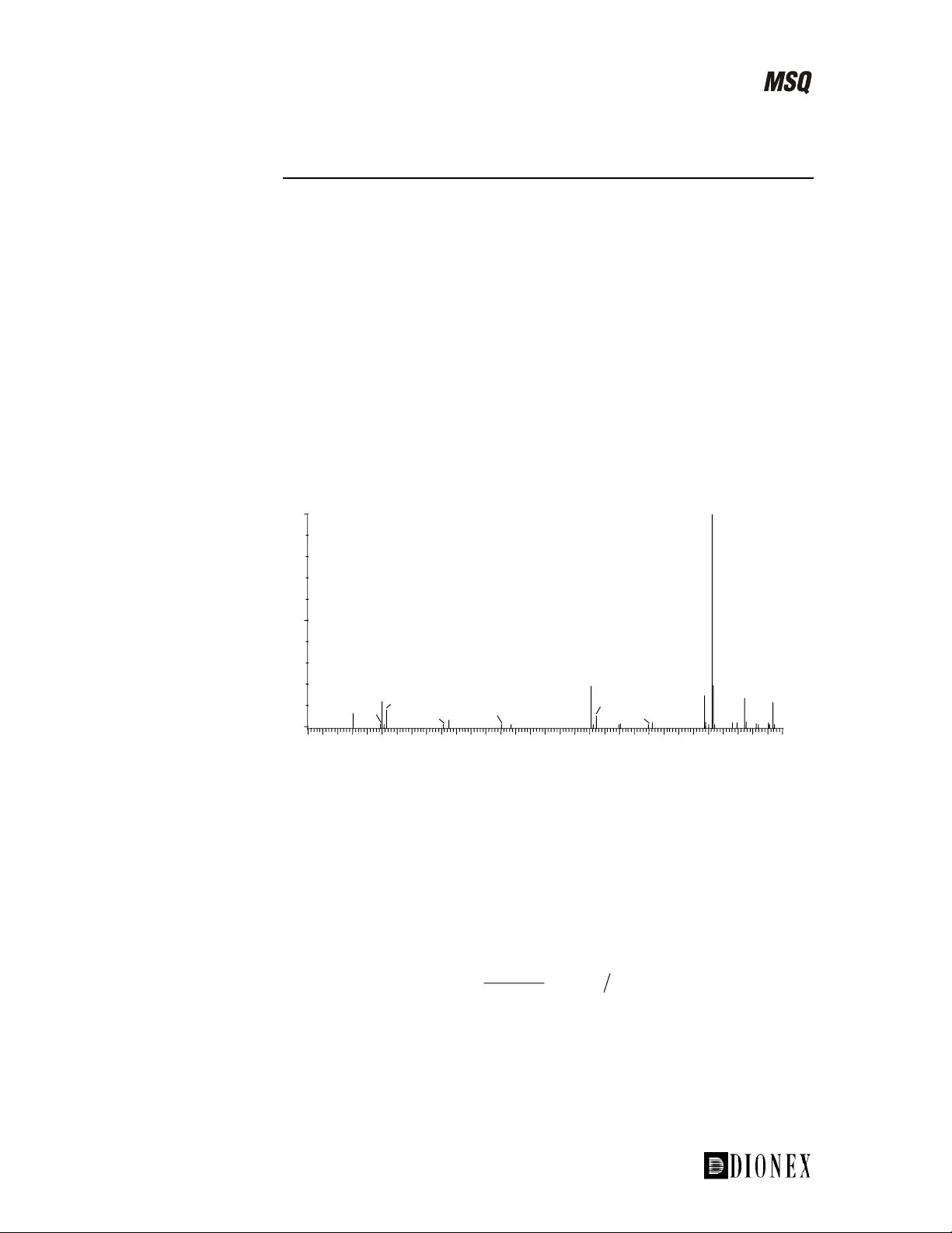
Centroid

During centroid acquisitions, Xcalibur automatically determines and saves the mass center of the acquired profile peak returned from the detector. Hence, the previously large number of points that described the mass spectral peak are reduced to a single centroid stick (see Figure 1-26) for each ion mass recorded. This has the advantage of reducing the quantity of data recorded to the hard disk and improving processing speeds.

100

120 140 160 180 200 220 240 260 280

265

267

263

Figure 1-26. Full scan centroid spectrum of pentachlorophenol

m/z

1-32 __________________________ MSQ Hardware Manual ____________________________

Page 37

Introducing the MSQ

_______________________________________________________________________The Data System

Profile

With profile acquisition, data is not “centroided” into sticks. Instead, the signal received by the interface electronics is stored to give an analog intensity profile of the data being acquired for every scan (see Figure 1-27). Profile acquisition enables mass spectral peak width and resolution to be examined and measured. For example, the resolution between an ion and its isotope(s) or multiply charged ions can be seen and measured, if necessary. This is most useful in the case of protein and peptide analysis, where multiply charged ions are formed.

As data is being written to disk at all times (even when there are no peaks being acquired), profile data acquisition places an extra burden on the acquisition system in comparison to centroided acquisition. Profile data files tend to be significantly larger than centroided ones and the scan speeds used tend to be slower than when acquiring centroided data.

100

281

283

275 300 325 350 375 400 425 450 475 500 525

325

Figure 1-27. Full scan profile spectrum of D-raffinose

503

504

m/z

___________________________MSQ Hardware Manual ___________________________ 1-33

Page 38

Introducing the MSQ The Data System ________________________________________________________________________

MCA

The third type of full scan acquisition is MCA. Such data can be thought of as “summed profile,” with only one intensity-accumulated scan being written to disk for a given experiment (see Figure 1-28). As each scan is acquired, its intensity data is added to the accumulated summed data of previous scans.

An advantage of MCA is that although noise will accumulate at the same rate as sample-related data, noise is random, and therefore its effects will be reduced over a number of scans. This will emphasize the sample-related data and improve signal to noise. A further advantage of MCA is that data is written to disk only at the end of an experiment; therefore, significantly less storage space is required.

MCA cannot be used for time-resolved data because an MCA raw file contains only one scan. Therefore, MCA is not used during a chromatographic run. Generally, it is used to acquire infusion or loop injected samples of fairly weak concentration (the signal can then be enhanced). The real-time spectrum can be viewed and the acquisition stopped when the required results are obtained. MCA is often used to acquire raw data from the infusion of proteins and peptides.

771

808

848

893

942

944

998

999

1060

1131

1212

1305

100

738

707

694

700 800 900 1000 1100 1200 1300

Figure 1-28. Full scan MCA spectrum of horse heart myoglobin

m/z

1-34 __________________________ MSQ Hardware Manual ____________________________

Page 39

Introducing the MSQ

_______________________________________________________________________The Data System

SIM Mode

This acquisition mode is used when only one or a few specific masses are to be monitored during the acquisition. Since most of the acquisition time is spent on these masses, the SIM technique is far more sensitive (typically greater than a factor of ten) than full scan techniques. However, this sensitivity does depend on the number of masses being monitored simultaneously.

SIM is also a highly selective technique. Impurities present in the sample that co-elute with the compound of interest will not affect the analysis as long as they do not produce ions at the same m/z value being monitored.

SIM does not produce spectra that can be used for library searching routines.

___________________________MSQ Hardware Manual ___________________________ 1-35

Page 40

Introducing the MSQ The Data System ________________________________________________________________________

1-36 __________________________ MSQ Hardware Manual ____________________________

Page 41

Chapter 2

Changing Ionization Modes 2.

Changing Ionization Modes ......................................................................................................2-i

Introduction ....................................................................................................................................2-1

Switching from ESI to APCI ..........................................................................................................2-2

Switching from APCI to ESI ..........................................................................................................2-4

____________________________MSQ Hardware Manual _____________________________ 2-i

Page 42

Changing Ionization Modes Introduction ____________________________________________________________________________

2-ii ____________________________ MSQ Hardware Manual ____________________________

Page 43

Changing Ionization Modes

____________________________________________________________________________ Introduction

Introduction

Use the information in this chapter in conjunction with the animations on the MSQ CD shipped with your system. The chapter is divided into the following sections:

Switching from ESI to APCI •

• Switching from APCI to ESI

____________________________MSQ Hardware Manual ____________________________ 2-1

Page 44

Changing Ionization Modes Switching from ESI to APCI ________________________________________________________________

Switching from ESI to APCI

The starting point for this procedure is the source setup for ESI operation, with the LC and gas flows off, and the probe cooled.

WARNING. Allow the source block and probe heater assembly to cool before changing ionization modes.

Unscrew and remove the PEEK finger-tight fitting from the ESI probe assembly (P/N FM102595).

Turn the locking plate clockwise to the open position, and remove the ESI probe assembly (P/N FM102595).

PEEK fitting

Figure 2-5. ESI probe assembly

Swap the ESI probe assembly (P/N FM102595) with the APCI probe

Locking plate

assembly (P/N FM102587), located in the holder in the door.

Turn the locking plate on the APCI probe assembly clockwise into the open position, insert the APCI probe assembly (P/N FM102587), and turn the locking plate counterclockwise into the closed position.

Change the APCI blank plug (P/N FM101437) with the APCI corona pin (P/N FM101433), located in the holder in the source enclosure door.

2-2 ___________________________ MSQ Hardware Manual ____________________________

Page 45

Changing Ionization Modes

________________________________________________________________Switching from ESI to APCI

Figure 2-6. APCI corona pin and APCI blank plug

6. Insert the PEEK finger-tight fitting into the APCI probe assembly (P/N

FM102587) and screw it into place.

____________________________MSQ Hardware Manual ____________________________ 2-3

Page 46

Changing Ionization Modes Switching from APCI to ESI ________________________________________________________________

Switching from APCI to ESI

The starting point for this procedure is the source setup for APCI operation, with the LC and gas flows off, and the probe cooled.

WARNING. Allow the source block and probe heater assembly to cool before changing ionization modes.

Unscrew and remove the PEEK finger-tight fitting from the APCI probe assembly (P/N FM102587).

Change the APCI blank plug (P/N FM101437) with the APCI corona pin (P/N FM101433), located in the holder in the source enclosure door.

Figure 2-7. APCI blank plug and APCI corona pin

3. Turn the locking plate clockwise to the open position, and remove the APCI probe assembly (P/N FM102587).

2-4 ___________________________ MSQ Hardware Manual ____________________________

Page 47

Changing Ionization Modes

________________________________________________________________Switching from APCI to ESI

PEEK fitting

Figure 2-5. ESI probe assembly

Swap the APCI probe assembly (P/N FM102587) with the ESI probe

Locking plate

assembly (P/N FM102595), located in the holder in the door.

Turn the locking plate on the ESI probe assembly clockwise into the open position, insert the ESI probe assembly (P/N FM102595), and turn the locking plate counterclockwise into the closed position.

Insert the PEEK finger-tight fitting into the ESI probe assembly (P/N FM102595) and screw it into place.

____________________________MSQ Hardware Manual ____________________________ 2-5

Page 48

Changing Ionization Modes Switching from APCI to ESI ________________________________________________________________

2-6 ___________________________ MSQ Hardware Manual ____________________________

Page 49

Chapter 3

LC/MS and the Cone Wash 3.

LC/MS and the Cone Wash ......................................................................................................3-i

Introduction ....................................................................................................................................3-1

LC/MS Considerations ...................................................................................................................3-2

Flow Rates .........................................................................................................................3-2

HPLC Solvents and Mobile Phase Additives ....................................................................3-3

Setting Up the Cone Wash..............................................................................................................3-7

Flow Splitting .................................................................................................................................3-9

___________________________ MSQ Hardware Manual _____________________________ 3-i

Page 50

LC/MS and the Cone Wash Introduction ____________________________________________________________________________

3-ii____________________________ MSQ Hardware Manual ____________________________

Page 51

LC/MS and the Cone Wash

____________________________________________________________________________ Introduction

Introduction

Historically, LC/MS has been compatible only with volatile buffer systems using modifiers such as trifluoroacetic acid, formic acid, and acetic acid. Phosphate buffers, although extensively used in LC separations, were not suited to LC/MS due to the rapid blocking of the ion sampling region caused by the deposition of involatile phosphate salts. The self-cleaning API source allows routine LC/MS with chromatographic buffers such as phosphates or ion-pairing agents and samples in dirty matrices.

This chapter contains the following information:

Details of HPLC solvents and mobile phase additives that focus on

•

LC/MS applications using the MSQ.

• • Instructions on how to set up the cone wash and information on when to

use it.

Instructions on flow splitting for use with hyphenated detection applications.

____________________________MSQ Hardware Manual ____________________________ 3-1

Page 52

LC/MS and the Cone Wash LC/MS Considerations ____________________________________________________________________

LC/MS Considerations

This section discusses the considerations to be taken into account when choosing solvents and additives. It also provides guidance on how to optimize LC/MS analyses to produce high quality data using the MSQ.

Flow Rates

In general, the column in use determines the flow rate. Each column has an optimum flow rate. The guidelines in Table 3-1 apply.

Table 3-1. LC columns and flow rates

Column ID Flow Rate

4.6 mm 1.0 mL/min

3.9 mm 0.5 mL/min

2.1 mm 0.2 mL/min

1.0 mm 40-50 µL/min

Capillary <10 µL/min

The different ionization modes require different flow rates and column IDs. The following guidelines apply when using the MSQ:

Electrospray can operate at all the flow rates described in Table 3-1.

•

Therefore, the full range of column IDs can be used without splitting the flow.

• APCI cannot operate at flow rates below 0.2 mL/min; therefore, suitable column IDs are 2.1 mm, 3.9 mm, and 4.6 mm.

3-2 ___________________________ MSQ Hardware Manual ____________________________

Page 53

LC/MS and the Cone Wash

____________________________________________________________________LC/MS Considerations

HPLC Solvents and Mobile Phase Additives

The following section is a guide for the choice of solvent and mobile phase additives to use. The choice of solvents for LC will be dictated primarily by the separation requirements, but there are some guidelines that need to be followed. These guidelines take the form of selected examples, which have been divided into three categories: most compatible, least suitable, and other less common ones. In all cases, degassed solvents are necessary for LC/MS operation. Sonication, helium sparging, or vacuum membrane degassing achieves this. Helium sparging and vacuum membrane degassing are the more efficient techniques.

Most Compatible Solvents

Most compatible solvents are:

Water •

• • Acetonitrile

Methanol

These common reverse phase LC solvents are ideal for LC/MS. When using high percentages of water, the probe temperature usually needs to be raised to aid desolvation in the source.

Most Compatible Additives

The most compatible additives are:

Acetic acid or formic acid •

LC separations can be enhanced by reducing the pH of the mobile phase. Suitable additives for this are acetic acid or formic acid. (Formic acid is stronger than acetic acid and therefore, less needs to be added to reach a required pH.) Addition of acids can suppress ionization in negative ion analysis and weakly acidic compounds may not form [M-H]- ions in acidic conditions.

•

Ammonium hydroxide

Ammonium hydroxide (ammonia solution) is suitable for increasing the pH of the mobile phase, which can enhance LC separations. When analyzing weakly acidic compounds, in negative ion mode, it is unlikely that there will be any suppression of ionization.

____________________________MSQ Hardware Manual ____________________________ 3-3

Page 54

LC/MS and the Cone Wash LC/MS Considerations ____________________________________________________________________

Ammonium acetate or ammonium formate •

These volatile salts are often used to buffer mobile phases. Use as little ammonium acetate or ammonium formate as possible, keeping the concentration below 100 mM. Ensure that the cone wash is running when using high concentrations.

•

Non-volatile salts

When using non-volatile salts, ensure that the cone wash is running as they can crystallize in the source, block the entrance cone, and prevent the mass spectrometer from functioning. The most common non-volatile salts used are phosphates.

•

Ion pairing agents

Ensure that the cone wash is running when using ion-pairing agents (for example, sodium octanesulfonic acid). Many ion-pairing agents suppress electrospray ionization.

Least Suitable Additives

Least suitable additives are surface-active agents/detergents.

These can suppress the ionization of other compounds. Detergents, by their very nature, are concentrated at the surface of a liquid. This causes problems with electrospray, as the ionization relies on the evaporation of ions from the surface of a droplet. The detergent therefore suppresses the evaporation of other ions. Use surfactants only when they are being analyzed themselves, not as additives to HPLC mobile phases.

Other Solvents

Other solvents are:

Normal phase solvents •

Normal phase solvents such as dichloromethane, hexane, and toluene are most suitable for use in APCI.

•

Propan-2-ol (IPA), 2-methoxyethanol, ethanol, and so on

These have all been used with LC/MS, but their use tends to be applicationspecific.

•

Dimethyl sulfoxide (DMSO)

This solvent is commonly used by synthetic chemists for primary dilution.

3-4 ___________________________ MSQ Hardware Manual ____________________________

Page 55

LC/MS and the Cone Wash

____________________________________________________________________LC/MS Considerations

Other Additives

•

Trifluoroacetic acid (TFA)

This is frequently used for peptide and protein analysis. High levels, >0.1% v/v, can cause suppression of sensitivity in positive ion mode. TFA may completely suppress ionization in negative ion mode.

•

Triethylamine (TEA)

This may suppress the ionization of less basic compounds in positive ion mode (as it also is readily ionized to give a [M+H]

ion at m/z 102). TEA enhances ionization of other compounds in negative ion mode because it is basic. This is a particularly useful additive for the analysis of nucleic acids.

•

Tetrahydrofuran (THF)

In ESI, use of THF can reduce sensitivity. This effect can be counteracted by post-column addition of ammonium acetate. It has no effect in APCI.

Caution. Do not use a concentration of THF greater than 5% with PEEK tubing. THF causes swelling in the PEEK tubing and consequently presents a risk of the LC tubing bursting.

• Inorganic acids

Inorganic acids (for example, sulfuric acid or phosphoric acid) can be used. Check the suitability of the LC column to low pHs.

Caution. After using phosphoric acid, thoroughly clean the source, source enclosure, and hexapole RF lens to minimize the physical damage.

____________________________MSQ Hardware Manual ____________________________ 3-5

Page 56

LC/MS and the Cone Wash LC/MS Considerations ____________________________________________________________________

Summary of Additives

Table 3-2. Summary of additive use

Avoid

Use

Positive ion Trifluoroacetic acid (TFA) (>0.1% v/v),

surfactants.

Negative ion Surfactants, organic acids; for example,

acetic acid, formic acid, trifluoroacetic acid (TFA).

Positive ion Acetic acid, formic acid, ammonium

acetate (<0.1M).

Negative ion Triethylamine (TEA), ammonium

hydroxide (ammonia solution), ammonium acetate (<0.1M).

3-6 ___________________________ MSQ Hardware Manual ____________________________

Page 57

LC/MS and the Cone Wash

________________________________________________________________ Setting Up the Cone Wash

Setting Up the Cone Wash

Use the following information in conjunction with the setup and maintenance animations on the MSQ CD shipped with the instrument.

Note. It is necessary to use the cone wash only for dirty matrices or with involatile buffers. Choose the cone wash solvent to give the most effective solubility for the expected contaminants.

A pump (such as the optional AXP-MS pump) delivers solvent to the cone wash. The PEEK tubing (green stripe is recommended) is fed through the door and attached to a PEEK fitting which screws into the instrument on the right of the source block cover (see Figure 3-1). The recommended flow rate is 100 µl/min with 50:50 methanol:water.

From LC pump to cone wash

Figure 3-1. Cone wash solvent delivery

Turn the cone wash nozzle counterclockwise until the tip of the nozzle just touches the top of the entrance cone, and then turn on the LC pump.

____________________________MSQ Hardware Manual ____________________________ 3-7

Page 58

LC/MS and the Cone Wash Setting Up the Cone Wash_________________________________________________________________

Figure 3-2. Cone wash nozzle in the on position

Caution. Do not leave the cone wash running when the source heater is turned off; this could lead to cone wash solvents condensing on the RF lens.

3-8 ___________________________ MSQ Hardware Manual ____________________________

Page 59

LC/MS and the Cone Wash

___________________________________________________________________________ Flow Splitting

Flow Splitting

Due to the MSQ’s source design, flow splitting of the LC eluent is not usually required. However, if hyphenated detection is required, flow splitting can be achieved in the following way.

Zero dead volume T-piece

HPLC column

PEEK LC tubing

PTFE sleeve

Fused silica

to waste or UV

Figure 3-7. Schematic of a split

Fused silica

to insert and source

PTFE sleeve

A simple and effective way to make a post-column split for use with the MSQ is shown in Figure 3-7.

Connect a zero dead volume T-piece to the exit of the column, using the normal PEEK or stainless steel LC tubing (PEEK tubing is used in the figure).

Connect one of the exits of the T-piece to the source enclosure, using narrow bore PEEK tubing or, as shown in the diagram, fused silica. Use a PTFE, or orange stripe PEEK tubing, sleeve to secure the fused silica into the T-piece.

Connect a length of the same tubing to the other exit (the split stream).

The amount of liquid directed through the split stream is determined by the backpressure exerted at this exit, and hence by the internal diameter and the length of the tubing attached. As a general rule, the longer the piece of tubing attached to the split, the greater the flow to the source and the smaller the split. To reduce the flow to the source and increase the split, shorten the length of tubing at the split stream exit.

There are a number of ways to measure the amount of liquid flowing into the source and hence measure the split ratio. Two methods are provided here; one gives a rough estimate and the other a more accurate figure.

____________________________MSQ Hardware Manual ____________________________ 3-9

Page 60

LC/MS and the Cone Wash Flow Splitting ___________________________________________________________________________

To achieve a rough estimate of the flow rate into the source:

Remove the probe from the source enclosure.

Connect the probe directly to the column outlet and set the flow rate of the LC pump to the desired flow rate into the source; for example,

0.2 mL/min.

Count the drops that fall off the end of the insert in one minute. Make a note of this figure.

Connect the split as shown in Figure 3-7.

Now set the LC pump to the flow rate that is required through the

5. column, for example, 1.0 mL/min.

Count the drops that fall off the end of the insert in one minute.

If the split is set up correctly (in this case, to give a split ratio of 4:1), then the number of drops recorded in Step 6 will be the same as that in Step 3. If the number of drops is greater in Step 6, shorten the length of the tubing connected to the waste (or UV detector) stream. If there are fewer drops in Step 6, then a longer length of tubing is required. Continue this until the number of drops in Step 6 is the same as that recorded in Step 3.

Note. There is no need to measure the split ratio accurately. Even significant changes in split ratio have only a minimal effect on chromatographic peak shape.

To accurately measure the split and therefore know the exact flow rate into the source, use the following method:

Remove the probe from the source enclosure.

Connect the split to the probe and LC pump as shown in Figure 3-7.

Set the flow rate of the pump to the flow required through the column; for example, 1.0 mL/min.

Collect and weigh the liquid that emerges from the insert in one minute.

Follow the same procedure with the liquid that emerges from the waste

5. (or UV detector) stream.

Calculate the ratio of the two masses of the liquid to give the split ratio,

6. and hence calculate the exact flow rate into the source.

For example, if 200 mg emerges from the insert and 800 mg from the waste stream in one minute, then the split ratio is 4:1 and the flow rate into the source can be calculated as 0.2 mL/min.

3-10 __________________________ MSQ Hardware Manual ____________________________

Page 61

Chapter 4

Reference Inlet System 4.

Reference Inlet System ..............................................................................................................4-i

Introduction ....................................................................................................................................4-1

Overview ........................................................................................................................................4-2

Setting Up the Reference Inlet System...........................................................................................4-3

____________________________MSQ Hardware Manual _____________________________ 4-i

Page 62

Reference Inlet System Introduction ____________________________________________________________________________

4-ii ____________________________ MSQ Hardware Manual ____________________________

Page 63

Reference Inlet System

____________________________________________________________________________ Introduction

Introduction

The MSQ’s built-in reference inlet system allows easy calibration and tuning.

This chapter provides instructions on how to set up the reference inlet system.

____________________________MSQ Hardware Manual ____________________________

4-1

Page 64

Reference Inlet System Overview ______________________________________________________________________________

Overview

The recommended way to introduce a sample for tuning and mass calibration is to use the reference inlet system. This method provides a steady flow of sample directly into the source (typically at flow rates of <50 µL/min).

Note. Calibration should be performed in positive electrospray mode.

4-2 ___________________________ MSQ Hardware Manual ____________________________

Page 65

Reference Inlet System

_______________________________________________________ Setting Up the Reference Inlet System

Setting Up the Reference Inlet System

Use the following information in conjunction with the setup and maintenance animations on the MSQ CD shipped with the instrument.

These instructions show how to configure the reference inlet system to introduce tuning and mass calibration samples into the source. They assume that the source is set up for electrospray ionization. If your source is not set up for ESI, refer to the chapter Changing Ionization Modes.

1. Ensure that there is calibrant in the calibration reference bottle. If not, unscrew the calibration reference bottle (P/N FM102771), fill it with calibrant, and screw it back into place.

Figure 4-2. Calibration reference bottle

2. Check the waste bottle (P/N FM102770). If it is full, unscrew it, empty it, and then screw it back into place.

Figure 4-2. Waste bottle

Check that liquid is emerging into the waste bottle.

Ideally, the instrument should already be in operate with the gas flow on. If it is not, the software will turn on the gas and put the instrument into operate.

Click, with the right mouse button, on the server icon and select Instrument Tune and Calibration… from the menu displayed. The Instrument Tuning and Calibration dialog box is displayed.

____________________________MSQ Hardware Manual ____________________________

4-3

Page 66

Reference Inlet System Setting Up the Reference Inlet System _______________________________________________________

Figure 4-2. Instrument Tuning and Calibration dialog box

6. Select Full System Autotune and click the Next button. A complete system tune will be performed, followed by a mass scale calibration. A series of messages will be displayed, informing you of the progress. To print a report, click the Print Report button.

Note. Allow time for the probe heater to warm up and stabilize at the required temperature before beginning autotune and calibration.

4-4 ___________________________ MSQ Hardware Manual ____________________________

Page 67

Reference Inlet System

___________________________________________________________ Standard Mass Scale Calibration

Standard Mass Scale Calibration

If there is a significant change in the observed masses, you may wish to perform a standard mass scale calibration.

1. Ensure that there is calibrant in the calibration reference bottle. If not, unscrew the calibration reference bottle (P/N FM102771), fill it with calibrant, and screw it back into place.

Figure 4-2. Calibration reference bottle

2. Check the waste bottle (P/N FM102770). If it is full, unscrew it, empty it, and then screw it back into place.

Figure 4-2. Waste bottle

Check that liquid is emerging into the waste bottle.

Ideally, the instrument should already be in operate with the gas flow on. If it is not, the software will turn on the gas and put the instrument into operate.

Click, with the right mouse button, on the server icon and select Instrument Tune and Calibration… from the menu displayed. The Instrument Tuning and Calibration dialog box is displayed.

____________________________MSQ Hardware Manual ____________________________

4-5

Page 68

Reference Inlet System Standard Mass Scale Calibration____________________________________________________________

Figure 4-2. Instrument Tuning and Calibration dialog box

6. Select Standard Mass Scale Calibration and click the Next button. A series of messages will be displayed, informing you of the progress. To print a report, click the Print Report button.

Note. Allow time for the probe heater to warm up and stabilize at the required temperature before beginning autotune and calibration.

4-6 ___________________________ MSQ Hardware Manual ____________________________

Page 69

Chapter 5

5. Routine and Preventive Maintenance

Routine and Preventive Maintenance ..................................................................................... 5-i

Introduction.................................................................................................................................... 5-1

Maintenance Schedule ................................................................................................................... 5-2

The Electrospray and APCI Probes ............................................................................................... 5-3

Flushing the Capillaries .................................................................................................... 5-3

ESI Probe Removal........................................................................................................... 5-4

ESI Probe Disassembly..................................................................................................... 5-5

Cleaning the ESI Probe..................................................................................................... 5-6

Replacing the Capillary..................................................................................................... 5-6

ESI Probe Assembly ......................................................................................................... 5-7

APCI Probe Removal........................................................................................................ 5-8

APCI Probe Disassembly.................................................................................................. 5-9

Cleaning the APCI Probe.................................................................................................. 5-9

Replacing the Capillary................................................................................................... 5-10

APCI Probe Assembly .................................................................................................... 5-10

The Source Block Assembly........................................................................................................ 5-11

Cleaning the Entrance Cone............................................................................................ 5-11

Cleaning the Cone Wash Nozzle .................................................................................... 5-13

Cleaning the Source Block Assembly............................................................................. 5-13

The Heater.................................................................................................................................... 5-21

Heater Removal .............................................................................................................. 5-21

Cleaning the Heater......................................................................................................... 5-21

Heater Replacement........................................................................................................ 5-22

The Rotary Pump ......................................................................................................................... 5-23

Checking the Rotary Pump Oil Level and Color ............................................................ 5-23

Changing the Rotary Pump Oil....................................................................................... 5-25

___________________________ MSQ Hardware Manual_____________________________ 5-i

Page 70

Routine and Preventive Maintenance Introduction ____________________________________________________________________________

5-ii____________________________ MSQ Hardware Manual ____________________________

Page 71

Routine and Preventive Maintenance

____________________________________________________________________________ Introduction

Introduction

The MSQ has been designed to be a low maintenance instrument. Apart from fairly light periodic preventive maintenance, the MSQ requires only simple source cleaning and inspection on a “loss of performance” basis.

This chapter contains details of how to perform all the user maintenance tasks on the MSQ, both routine and as required. Use this information in conjunction with the setup and maintenance animations on the MSQ CD shipped with the instrument.

The chapter begins with a maintenance schedule that indicates how often you should perform each routine maintenance task.

The chapter then describes maintenance of the following parts of the MSQ:

The electrospray and APCI inserts •

•

The source block

•

The RF lens

•

The heater

•

The rotary pump

____________________________MSQ Hardware Manual ____________________________

5-1

Page 72

Routine and Preventive Maintenance Maintenance Schedule____________________________________________________________________

Maintenance Schedule

Table 5-1 is a list of routine maintenance procedures that should be carried out on the MSQ at the intervals specified.

The maintenance schedule provides only a rough guide to the frequency of maintenance tasks. The appropriate frequency depends on instrument usage and the level of system-induced contamination from samples and matrices.

Table 5-1. Maintenance schedule

Frequency Action

Weekly Clean the source if a drop in sensitivity is seen during

analysis, or if there is a drop in sensitivity when performing the sensitivity verification test (refer to the chapter Preparing for Daily Operation in the MSQ Getting Started manual); see page 5-12.

Clean and flush the capillaries; see page 5-4.

Every 3-6 months

Clean the RF lens; see page 5-16.

Every 6 months

Check the oil level and color in the rotary pump and add oil if necessary; see page 5-23.

Replace the rotary pump oil; see page Error! Bookmark not defined..

Refer to the PC user guide supplied for cleaning the PC fan filters.

5-2 ___________________________ MSQ Hardware Manual ____________________________

Page 73

Routine and Preventive Maintenance

__________________________________________________________The Electrospray and APCI Probes

The Electrospray and APCI Probes

To extend their lifetime, regularly flush both the ESI and APCI probes with solvent, especially after prolonged use with buffers. The probes can also be stripped down and cleaned. Replace the capillaries if they become blocked.

Flushing the Capillaries

To prevent blockage, flush the capillaries with [50:50] acetonitrile:water or methanol:water after use with phosphates, ion-pairing agents, acids, or other additives. The probe does not need to be disassembled for this procedure, but it should be removed from the source block enclosure. Remove the probe from the source block, attach the probe to the pump (with the column removed), and flush the probe.

Note. To prevent blockage, flush each capillary after using buffers.

____________________________MSQ Hardware Manual ____________________________

5-3

Page 74

Routine and Preventive Maintenance The Electrospray and APCI Probes __________________________________________________________

ESI Probe Removal

WARNING. Allow the source block and probe heater assembly to cool before changing ionization modes.

Unscrew and remove the PEEK finger-tight fitting from the ESI probe assembly (P/N FM102595).

Turn the locking plate clockwise to the open position and remove the ESI probe assembly (P/N FM102595).

PEEK fitting

Figure 5-5. ESI probe assembly

Locking plate

5-4 ___________________________ MSQ Hardware Manual ____________________________

Page 75

Routine and Preventive Maintenance

__________________________________________________________The Electrospray and APCI Probes

ESI Probe Disassembly

The starting point for this procedure is the ESI probe removed from the instrument.

Using the 2.5 mm Allen key, unscrew the M3 x 10 cap head stainless steel screw (P/N FM103046).

Remove the probe clamp and locking plate.

Using the 10 mm spanner, unscrew the capillary retaining nut.

Remove the graphite ferrule (P/N 6070119), PEEK insert (P/N FM102591), and ESI probe capillary (P/N FM102698).

Caution. Exercise care when handling the ESI probe capillary because it is fragile and may be damaged easily.

Using the 2.5 mm Allen key, unscrew the two M3 x 8 cap head stainless steel screws (P/N 5313020).

Remove the ESI probe mount and O-rings.

Remove the ESI ceramic sleeve (P/N FM103394) from the ESI ceramic probe assembly.

____________________________MSQ Hardware Manual ____________________________

5-5

Page 76

Routine and Preventive Maintenance The Electrospray and APCI Probes __________________________________________________________

Cleaning the ESI Probe

The ESI probe can be stripped down for thorough cleaning after prolonged use with additives.

Wipe the surface of the stainless steel insert capillary with [50:50] methanol:water.

Sonicate the ceramic sleeve in concentrated nitric acid. Then boil it in distilled water for 5 to 10 minutes.

WARNING. Exercise extreme caution when using concentrated nitric acid. Always wear protective clothing and use only in a fume hood. Observe appropriate disposal requirements when discarding the used acid.

Replacing the Capillary

Replace the capillary if it has become blocked or partially blocked during operation. A significant increase in LC pump backpressure (that is, up to 300 psig at 1 mL/min added to the total LC system backpressure) or instability in the signal could be symptoms of a partially blocked capillary.

5-6 ___________________________ MSQ Hardware Manual ____________________________

Page 77

Routine and Preventive Maintenance

__________________________________________________________The Electrospray and APCI Probes

ESI Probe Assembly

The starting point for this procedure is a disassembled ESI probe.

Insert the ESI ceramic sleeve (P/N FM103394) into the ESI ceramic probe assembly.

Place the O-rings in position and insert the ESI probe mount.

Screw in the two M3 x 8 cap head stainless steel screws (P/N 5313020) and tighten, using the 2.5 mm Allen key.

Insert the ESI probe capillary (P/N FM102698), graphite ferrule (P/N

6070119), and PEEK insert (P/N FM102591).

Caution. Exercise care when handling the ESI probe capillary because it is fragile and may be damaged easily.

Screw in the capillary retaining nut until finger-tight.

Use the setting fixture depth plate to align the end of the ESI probe capillary and tighten the capillary retaining nut, using the 10 mm spanner.

Place the locking plate and probe clamp in position.

Screw in the M3 x 10 cap head stainless steel screw (P/N FM103046) and tighten, using the 2.5 mm Allen key.

____________________________MSQ Hardware Manual ____________________________

5-7

Page 78

Routine and Preventive Maintenance The Electrospray and APCI Probes __________________________________________________________

APCI Probe Removal

WARNING. Allow the source block and probe heater assembly to cool before changing ionization modes.

Unscrew and remove the PEEK finger-tight fitting from the APCI probe assembly (P/N FM102587).

Turn the locking plate clockwise to the open position and remove the APCI probe assembly (P/N FM102587).

PEEK fitting

Figure 5-5. APCI probe assembly

Locking plate

5-8 ___________________________ MSQ Hardware Manual ____________________________

Page 79

Routine and Preventive Maintenance

__________________________________________________________The Electrospray and APCI Probes

APCI Probe Disassembly

The starting point for this procedure is the APCI probe removed from the instrument.

Using the 2.5 mm Allen key, unscrew the M3 x 10 cap head stainless steel screw (P/N FM103046).

Remove the probe clamp and locking plate.

Using the 10 mm spanner, unscrew the capillary retaining nut.

Remove the graphite ferrule (P/N 6070119), PEEK insert (P/N FM102591), and APCI capillary tube (P/N FM102594).

Caution. Exercise care when handling the APCI probe capillary because it is fragile and may be damaged easily.

Using the 2.5 mm Allen key, unscrew the two M3 x 8 cap head stainless steel screws (P/N 5313020).

Remove the APCI probe mount and O-rings.

Cleaning the APCI Probe

The APCI probe can be stripped down for thorough cleaning after prolonged use with additives.

1. Wipe the surface of the stainless steel insert capillary with [50:50] methanol:water.

____________________________MSQ Hardware Manual ____________________________

5-9

Page 80

Routine and Preventive Maintenance The Electrospray and APCI Probes __________________________________________________________

Replacing the Capillary

APCI Probe Assembly

The starting point for this procedure is a disassembled APCI probe.

Place the O-rings in position and insert the APCI probe mount.

Screw in the two M3 x 8 cap head stainless steel screws (P/N 5313020) and tighten, using the 2.5 mm Allen key.

Insert the APCI capillary tube (P/N FM102594), graphite ferrule (P/N

6070119), and PEEK insert (P/N FM102591).

Caution. Exercise care when handling the APCI probe capillary because it is fragile and may be damaged easily.

Screw in the capillary retaining nut until finger-tight.

Use the setting fixture depth plate to align the end of the APCI probe capillary and tighten the capillary retaining nut, using the 10 mm spanner.

Place the locking plate and probe clamp in position.

Screw in the M3 x 10 cap head stainless steel screw (P/N FM103046) and tighten, using the 2.5 mm Allen key.

5-10 __________________________ MSQ Hardware Manual ____________________________

Page 81

Routine and Preventive Maintenance

_______________________________________________________________ The Source Block Assembly

The Source Block Assembly

The source block assembly can be removed from the instrument (see page 5-

12) and disassembled into its component parts for cleaning. Typically, the

entrance cone needs to be cleaned most frequently because it becomes dirty with use over a long period. The cone can be reached without the need to remove the source block from the instrument.

WARNING. Allow the source block and probe heater assembly to cool before carrying out any maintenance.

Cleaning the Entrance Cone

Probe

Figure 5-4. Exposing the entrance cone

Vent the instrument if it is currently under vacuum. Right-click on the server and choose Vent.

Remove the PEEK fitting from the APCI or ESI probe assembly, turn the locking plate clockwise into the open position, and remove the probe assembly. See ESI Probe Removal or APCI Probe Removal.

If the cone wash is in use, switch the cone wash pump off and turn the cone wash nozzle until it is clear of the entrance cone.

If in APCI mode, change the APCI corona pin with the APCI blank plug (located in the source enclosure door).

____________________________MSQ Hardware Manual ___________________________

PCI corona pin Cone wash nozzle

5-11

Page 82

Routine and Preventive Maintenance The Source Block Assembly _______________________________________________________________

Turn the entrance cone assembly (P/N FM103412) clockwise and pull forward to remove it.

Using a 2.5 mm screwdriver, remove the entrance cone O-ring (P/N FM100231).

Caution. Exercise great care when handling the entrance cone. Always store with the cone facing upwards.

Note. To prevent the cone being damaged, it is recommended that you place a clean lint-free cloth in the beaker and use tweezers to handle the entrance cone.

7. Sonicate the cone, first in a 10% v/v solution of formic acid and then in methanol.

Caution. Do not sonicate the O-ring, as the solvent and acid may damage them.

Replace the O-ring.

For heavy buildup that is not removed by the steps above, use the 12 micron lapping paper.

10.

Take a small piece of the lapping paper and fold over, but do not crease it to a point. This prevents too much pressure being applied to the cone orifice.

11.

Rub the outside of the cone with the lapping paper until the buildup has been removed.

12.

Replace the entrance cone assembly and turn counterclockwise until locked in place.

13.

Reinsert the probe and PEEK fitting.

5-12 __________________________ MSQ Hardware Manual ____________________________

Page 83

Routine and Preventive Maintenance

_______________________________________________________________ The Source Block Assembly

Cleaning the Cone Wash Nozzle

The cone wash nozzle (P/N FM102521) should require cleaning only if it becomes blocked. When the pump supplying the cone wash with solvent is switched on, check the backpressure; if it rises, this could indicate a blockage in the nozzle.

Remove the entrance cone. See Cleaning the Entrance Cone on page 5-

11.

Remove the cone wash nozzle and sonicate, first in a 10% v/v solution of formic acid and then in methanol.

Replace the nozzle and entrance cone.

Cleaning the Source Block Assembly

It is good practice to clean the entire source block assembly on a weekly basis, particularly if complex sample matrices or chromatographic buffers are routinely used.

Carry out the procedure for removing the source block assembly and then the procedure for disassembling and cleaning the source block if the source has become completely blocked.

From the animations main menu, choose RF Lens Disassembly, Cleaning, and Assembly. Follow the procedure for RF Lens Removal and then RF Lens Disassembly, or follow the Full RF Lens Cleaning Procedure.

Removing the Source Block Assembly

The starting point for this procedure is the source setup for ESI or APCI operation, with the LC and gas flows off, and the probe cooled.

WARNING. Allow the source block and probe heater assembly to cool before carrying out any maintenance.

Vent the instrument if it is currently under vacuum. Right-click on the server and choose Vent.

Unscrew and remove the PEEK finger-tight fitting from the ESI probe assembly (P/N FM102595) or APCI probe assembly (P/N FM102587).

Turn the locking plate clockwise to the open position and remove the ESI probe assembly (P/N FM102595) or APCI probe assembly (P/N FM102587).

____________________________MSQ Hardware Manual ___________________________

5-13

Page 84

Routine and Preventive Maintenance The Source Block Assembly _______________________________________________________________

PEEK fitting

Locking plate

Figure 5-5. ESI probe assembly and source block enclosure

If in APCI mode, change the APCI corona pin (P/N FM101433) with

APCI blank plug

Entrance cone

Cone wash nozzle

the APCI blank plug (P/N FM101437), located in the holder in the source enclosure door.

If the cone wash is in use, switch off the cone wash pump and turn the cone wash nozzle until it is clear of the entrance cone.

Turn the entrance cone assembly (P/N FM103412) clockwise and pull forward to remove it.

Remove the cone wash nozzle (P/N FM102521).

Loosen the thumbscrews on the source block and pull out the source block assembly (P/N FM102573).

Source block

Thumbscrews

Figure 5-5. Removing the source block assembly

5-14 __________________________ MSQ Hardware Manual ____________________________

Page 85

Routine and Preventive Maintenance

_______________________________________________________________ The Source Block Assembly

Disassembling the Source Block Assembly

The starting point for this procedure is the source block assembly removed from the MSQ.

WARNING. Allow the source block and probe heater assembly to cool before carrying out any maintenance.

Figure 5-6. Source block assembly

Unscrew the three spring screws at the base of the RF lens and remove the RF lens.

Remove the hexapole screw insulator (P/N FM102248), extraction cone (P/N FM102263), and extraction cone insulator (P/N FM102264).

Remove the three O-rings: top left O-ring 7 x 3 Viton® degas (P/N FM102655), bottom left O-ring BS207 Viton degas (P/N FM101417), and right O-ring BS225 Viton degas (P/N FM103048).

Using the 6 mm screwdriver, unscrew the two sealing plugs (P/N FM102277) and remove the two O-rings (one at each side of the source block).

Using the sump lever tool, unscrew the source block sealing plug (P/N FM101460).

____________________________MSQ Hardware Manual ___________________________

5-15

Page 86

Routine and Preventive Maintenance The Source Block Assembly _______________________________________________________________

Cleaning the Source Block

1. Sonicate the disassembled component parts (except the O-rings) first in a 1% v/v solution of formic acid, then in water, and then in methanol.

Caution. Ensure that the parts do not become damaged in this process. If necessary, sonicate each part separately. In particular, ensure that the cones are face-up at all times.

Caution. Do not sonicate the O-rings, as the solvent and acid may damage them.

Cleaning the RF Lens

Under normal working conditions, this procedure needs to be carried out approximately once every 3 to 6 months. Refer to the Maintenance

Schedule topic on page 5-2.

WARNING. Allow the source block and probe heater assembly to cool

before carrying out any maintenance.

1. Totally immerse the RF lens in a measuring cylinder or beaker of [50:50] methanol:water and sonicate.

5-16 __________________________ MSQ Hardware Manual ____________________________

Page 87

Routine and Preventive Maintenance

_______________________________________________________________ The Source Block Assembly

Figure 5-7. Cleaning the RF Lens

Caution. To prevent the RF lens from touching the bottom of the vessel and hence becoming damaged, either suspend it on a wire or place a tissue at the bottom of the vessel.

If necessary, clean the differential aperture plate with a cotton bud (Q-tip) soaked in [50:50] methanol:water.

Rinse the RF lens with methanol and dry with nitrogen gas.

____________________________MSQ Hardware Manual ___________________________

5-17

Page 88

Routine and Preventive Maintenance The Source Block Assembly _______________________________________________________________

Assembling the Source Block Assembly

The starting point for this procedure is the disassembled source block assembly.

Figure 5-8. Source block assembly

Screw in the source block sealing plug (P/N FM101460). Tighten, using the sump lever tool.

Insert the sealing plug O-rings and screw in the two sealing plugs (P/N FM102277), using the 6 mm screwdriver. (There is one plug and O-ring at each side of the source block.)

Replace the three O-rings: top left O-ring 7 x 3 Viton degas (P/N FM102655), bottom left O-ring bs207 Viton degas (P/N FM101417), and right O-ring bs225 Viton degas (P/N FM103048).

Replace the extraction cone insulator (P/N FM102264), extraction cone (P/N FM102263), and hexapole screw insulator (P/N FM102248).

Replace the RF lens and screw in the three spring screws at the base of the RF lens.

5-18 __________________________ MSQ Hardware Manual ____________________________

Page 89

Routine and Preventive Maintenance

_______________________________________________________________ The Source Block Assembly

Replacing the Source Block Assembly

The starting point for this procedure is the source block assembly removed from the MSQ.

Source bloc

Thumbscrews

Figure 5-5. Replacing the source block assembly

Push the source block assembly (P/N FM102573) into place in the source block enclosure and tighten the thumbscrews on the source block.

Replace the cone wash nozzle (P/N FM102521).

Replace the entrance cone assembly (P/N FM103412) and turn counterclockwise.

Turn the locking plate clockwise to the open position and insert the ESI probe assembly (P/N FM102595) or APCI probe assembly (P/N FM102587).

Turn the locking plate counterclockwise into the closed position.

Screw the PEEK fitting finger-tight into the ESI probe assembly (P/N FM102595) or APCI probe assembly (P/N FM102587).

____________________________MSQ Hardware Manual ___________________________

5-19

Page 90

Routine and Preventive Maintenance The Source Block Assembly _______________________________________________________________

PEEK fitting

Locking plate APCI blank plug Entrance cone Cone wash nozzle

Figure 5-5. ESI probe assembly and source block enclosure

Cleaning the Extraction Cone

The starting point for this procedure is the source block assembly removed from the MSQ and disassembled.

Caution. Exercise great care when handling the extraction cone. Always store with the cone facing upward.

Note. To prevent the cone being damaged, it is recommended that you place a clean lint-free cloth in the beaker and use tweezers to handle the extraction cone.

1. Sonicate the cone, first in a 10% v/v solution of formic acid and then in methanol.

5-20 __________________________ MSQ Hardware Manual ____________________________

Page 91

Routine and Preventive Maintenance

_____________________________________________________________________________The Heater

The Heater

If the instrument is used primarily in APCI mode, it is recommended that the heater be cleaned on a monthly basis. If used in ESI mode, the heater will need cleaning less frequently.

Heater Removal

The starting point for this procedure is the source setup for ESI or APCI operation, with the LC and gas flows off, and the probe cooled.

WARNING. Allow the source block and probe heater assembly to cool before performing any maintenance.

Remove the ESI or APCI probe. See ESI Probe Removal or APCI Probe Removal.

Remove the source block cover.

Disconnect the heater connectors.

Using the 2.5 mm Allen key, unscrew the two M3 x 10 cap head stainless steel screws (P/N FM103046). Remove the screws and the screw insulators.

Remove the heater assembly (P/N FM102576).

Cleaning the Heater

Clean the inside of the heater tube with a cotton bud (Q-tip™) soaked in [50:50] methanol:water.

For heavy contamination, the heater tube can be sonicated in a 1% v/v solution of formic acid.

Caution. If you are sonicating the heater, you must immerse only the tube part of the heater. Damage will occur if any other part of the heater comes into contact with the formic acid solution.

____________________________MSQ Hardware Manual ___________________________

5-21

Page 92

Routine and Preventive Maintenance The Heater _____________________________________________________________________________

Heater Replacement

The starting point for this procedure is the heater assembly removed from the MSQ.

Insert the heater assembly (P/N FM102576).

Screw in the M3 x 10 cap head stainless steel screw (P/N FM103046) and tighten, using the 2.5 mm Allen key

Insert the screw insulators and the two M3 x 10 cap head stainless steel screws (P/N FM103046). Tighten, using the 2.5 mm Allen key.

Push in the heater connectors.

Replace the source block cove.

Insert the ESI or APCI probe.

5-22 __________________________ MSQ Hardware Manual ____________________________

Page 93

Routine and Preventive Maintenance

_____________________________________________________________________ The Vacuum System

The Vacuum System

The vacuum system consists of two types of vacuum pumps: a turbomolecular pump and a rotary pump. The turbomolecular pump is housed within the MSQ and must be serviced only by a trained Dionex Service Representative. The rotary pump is external to the MSQ and requires routine maintenance to keep it running at its optimum performance level.

Maintaining the Fore Pump

The fore pump (the rotary or backing pump) is external to the MSQ and requires routine maintenance to keep it running at its optimum performance level. The pumps used for this purpose come from two manufacturers– Busch and Edwards. The type of pump on the system will depend on when the instrument was purchased. The Busch pump has external and internal filters that should be serviced at regular intervals. The Edwards pump does not have filters that require routine maintenance.

The following maintenance procedures are covered here:

Checking the rotary pump oil level and color •

•

Adding oil to top-up the oil level

•

Changing the rotary pump oil

•

Replacing the external oil filter (Busch pumps only)

Note: More information on operating and maintaining the rotary pump can be found in the Rotary Pump User Manual, supplied with the MSQ system.

Checking the Rotary Pump Oil Level and Color

Check the rotary pump oil level and color at least once a week.

If the oil level in the rotary pump gets low before the scheduled oil change, use the procedure in the next section to add oil.

To check the oil:

Look through the oil sight glass at one end of the rotary pump. The oil level should be between the upper and lower marks positioned next to the window.

If the oil level is near or below the lower mark, add more oil. Refer to the procedure for adding oil on page 5-24.

____________________________MSQ Hardware Manual ___________________________

5-23

Page 94

Routine and Preventive Maintenance The Vacuum System _____________________________________________________________________

If a six-monthly service is due, it may be more convenient to drain and replace the oil. In this case, refer to the procedure for changing the rotary pump oil on page 5-25.

Note: If the oil has turned dark in color, it should also be replaced. (Clean rotary pump oil is a clear straw color [Anderol 555] or almost colorless [UltraGrade 19].)

Adding Oil

WARNING: Vent the instrument before adding oil. Attempting to add oil while the pump is running could result in serious personal injury from hot rotary pump oil.

NOTE: Do not mix oil types The oil used in the Edwards Rotary Pump is type Ultragrade 19 (P/N 062746 or 062747). The oil used in the Busch Rotary Pump is type Anderol 555 (P/N 060124 or 060125).

Turn Operate Off and vent the instrument. Refer to the chapter Shutting

3. Down and Restarting the System for information on turning Operate Off and venting.

4. Remove the oil filler plug located above the oil sight glass, marked

, from the pump.

5. Pour the oil into the pump until the oil level in the oil sight glass is close to, but not above, the upper mark.

5-24 __________________________ MSQ Hardware Manual ____________________________

Page 95

Routine and Preventive Maintenance

_____________________________________________________________________ The Vacuum System

oil filter

oil filler plug

oil sight glass

oil drain plug

Figure 5-6. Busch Rotary pump

6. Replace the oil filler plug.

Changing the Rotary Pump Oil

The oil in the rotary pump should be replaced at least once every six months.

The oil used in the Busch Rotary Pump is Anderol 555 (P/N 061024 and

061025).

The oil used in the Edwards Rotary Pump is type Ultragrade 19 (P/N 062746 or 062747).

WARNING: Wear gloves when changing the oil. Avoid contact with the pump oil; it may contain dissolved toxic residues from analyzed samples. Observe appropriate disposal requirements when discarding the used oil.

Turn Operate Off and vent the instrument.

Elevate the rotary pump to gain access to the oil drain plug.

WARNING: The rotary pump is a heavy item and requires at least two people to lift and move it safely.

9. Place a container under the oil drain plug on the rotary pump (below the

oil sight glass, marked ).

____________________________MSQ Hardware Manual ___________________________

5-25

Page 96

Routine and Preventive Maintenance The Vacuum System _____________________________________________________________________

10. Remove the oil filler plug located above the oil sight glass, marked

, from the pump.

11.

Remove the drain plug from the pump and allow the old oil to drain out until it reaches a trickle.

12.

If the oil filter is to be replaced (Busch pump only), remove the old one (using the type of tool used for automobile filter removal) and fit a new one (FM103825).

13.

Replace the drain plug.

14.

Fill the pump reservoir up to, but not above, the upper mark.

15.

Replace the filler plug.

16.

Pump down the instrument to prepare for operation.

Note: Leave the system pumping for at least half an hour before beginning operation.

5-26 __________________________ MSQ Hardware Manual ____________________________

Page 97

Chapter 6

Troubleshooting 6.

Troubleshooting .........................................................................................................................6-i

Introduction ....................................................................................................................................6-1

Troubleshooting Help .....................................................................................................................6-2

Resolving Common Problems ........................................................................................................6-3

Checking the MSQ Power Supply Requirements..............................................................6-3

Restarting the PC...............................................................................................................6-3

HPLC System Troubleshooting......................................................................................................6-4

Buffers and Additives........................................................................................................6-4

Mobile Phase Reservoir.....................................................................................................6-4

Bubble Problems and Degassing ....................................................................................... 6-4

Contamination in the LC System.......................................................................................6-5

Tubing and Fittings............................................................................................................6-5

Injection Valves.................................................................................................................6-7

UV Detectors .....................................................................................................................6-7

Preventive Maintenance and Spares ..................................................................................6-9

____________________________MSQ Hardware Manual _____________________________ 6-i

Page 98

Troubleshooting Introduction ____________________________________________________________________________

6-ii____________________________ MSQ Hardware Manual ____________________________

Page 99

Troubleshooting

____________________________________________________________________________ Introduction

Introduction

This chapter helps you to diagnose and resolve problems that may occur from time to time with the MSQ LC/MS system.

If you encounter a problem that is not described here, or have a problem that is not resolved by the remedy suggested, contact your local Dionex Service Representative for assistance.

This chapter is divided into the following sections:

Troubleshooting Help

•

An introduction to the troubleshooting help system that assists in identifying the precise nature of the problem and the action to be taken.

• • Resolving Common Problems

This section provides procedures to help remedy some of the more easily resolved problems you might encounter.

HPLC System Troubleshooting

This section provides a general guide to HPLC system troubleshooting.

____________________________MSQ Hardware Manual ____________________________ 6-1

Page 100

Troubleshooting Troubleshooting Help _____________________________________________________________________

Troubleshooting Help

The troubleshooting help system is designed to help you identify problems in the following areas:

General system problems

•

Problems relating to the basic operation of the system; for example, breaks in power supply.

•

Low sensitivity

Problems relating to low sensitivity. The symptoms are divided into excessive noise, low signal, and no signal.

•

Inlet system/chromatography

Problems relating to liquid chromatography and the HPLC system.

•

Spectral problems

Problems relating to mass spectral data.

•

Calibration

Problems relating to calibration.

•

Tuning

Problems relating to tuning.

•

Communication

Problems relating to communications among the various parts of the system and with Xcalibur.

•

Vacuum

Problems relating to the vacuum system.

•

MS resolution

Problems relating to MS resolution.

The troubleshooting help system describes the visible symptoms, the probable cause of the problem, and suggestions on how to remedy it.

To open the troubleshooting help, double-click on the troubleshooting help desktop icon.

6-2 ___________________________ MSQ Hardware Manual ____________________________

Dionex MSQ User Manual

Specifications and Main Features

Frequently Asked Questions

User Manual

Introduction

System Overview

What Is Mass Detection?

Exterior Features of the MSQ

The Source–An Introduction to API Techniques

Electrospray

Atmospheric Pressure Chemical Ionization

Source Fragmentation

Cone Voltage Ramping

Polarity Switching

Application of API Techniques

The Self-Cleaning Source: Cone Wash

Introduction

Functional Description

The Reference Inlet System

Introduction

Functional Description

The Mass Analyzer and Detector

The Vacuum System

The Data System

Software

Raw Data

Raw Data Types

Introduction

Switching from ESI to APCI

Switching from APCI to ESI

Introduction

LC/MS Considerations

Flow Rates

HPLC Solvents and Mobile Phase Additives

Setting Up the Cone Wash

Flow Splitting

Introduction

Overview

Setting Up the Reference Inlet System

Standard Mass Scale Calibration

Introduction

Maintenance Schedule

The Electrospray and APCI Probes

Flushing the Capillaries

ESI Probe Removal

ESI Probe Disassembly

Cleaning the ESI Probe

Replacing the Capillary

ESI Probe Assembly

APCI Probe Removal

APCI Probe Disassembly

Cleaning the APCI Probe

Replacing the Capillary

APCI Probe Assembly

The Source Block Assembly

Cleaning the Entrance Cone

Cleaning the Cone Wash Nozzle

Cleaning the Source Block Assembly

The Heater

Heater Removal

Cleaning the Heater

Heater Replacement

The Vacuum System

Maintaining the Fore Pump

Changing the Rotary Pump Oil

Introduction

Troubleshooting Help