

Page 1

TI 385 (6.0 EN)
d&b Line array design, ArrayCalc V8.x
Page 2

Contents
1. Introduction..................................................4
2. The J-Series line array...................................4
2.1 Number of cabinets required............................................4
2.2 J-SUB subwoofer setup.......................................................4
2.2.1 J-SUB ground stacks........................................................5
2.2.2 J-SUBs flown on top of a J8/J12 array........................5
2.2.3 Flown J-SUB columns.......................................................5
2.2.4 J-SUB horizontal SUB array............................................5
2.3 J-SUB/J-INFRA subwoofer setup.......................................5
2.3.1 Combined J-INFRA/J-SUB ground stacks.....................5
2.3.2 Flown J-SUBs, J-INFRA ground stacks...........................5
2.3.3 Flown J-SUBs, J-INFRA SUB array.................................5
3. The V-Series line array..................................6
3.1 Number of cabinets required............................................6
3.2 V-SUB subwoofer setup......................................................6
3.2.1 V-SUB ground stacks.......................................................7
3.2.2 V-SUBs flown on top of a V8/V12 array.....................7
3.2.3 Flown V-SUB columns......................................................7
3.2.4 V-SUB horizontal SUB array..........................................7
3.3 V-, J-SUB/J-INFRA subwoofer setup..................................7
3.3.1 Combined J-, V-SUB ground stacks...............................7
3.3.2 Flown V-, J-SUBs or J-INFRA ground stacks..................7
3.3.3 Flown V-SUBs, J-INFRA SUB array................................7
4. The Y-Series line array..................................8
4.1 Number of cabinets required............................................8
4.2 Y-SUB subwoofer setup......................................................8
4.2.1 Y-SUB ground stacks.......................................................9
4.2.2 Y-SUBs flown on top of a Y8/Y12 array.....................9
4.2.3 Flown Y-SUB columns......................................................9
4.2.4 Y-SUB horizontal SUB array...........................................9
4.3 V-, Y-, J-SUB/J-INFRA subwoofer setup............................9
4.3.1 Combined J-, Y-SUB ground stacks...............................9
4.3.2 Flown Y-, J-SUBs or J-INFRA ground stacks..................9
4.3.3 Flown Y-SUBs, J-INFRA SUB array................................9
5. The Q-Series line array................................10
5.1 Number of cabinets required..........................................10
5.2 Subwoofer setup...............................................................10
6. The T-Series line array.................................12
6.1 Number of cabinets required..........................................12
6.2 Subwoofer setup...............................................................12
7. The xA-Series line array..............................13
7.1 Number of cabinets required..........................................13
7.2 Subwoofer setup...............................................................13
8. The d&b point sources.................................14
8.1 Number of cabinets required..........................................14
9. Column loudspeakers..................................14
10. ArrayCalc..................................................15
10.1 ArrayCalc installation....................................................15
10.2 Starting ArrayCalc.........................................................15
10.3 ArrayCalc menu options and Toolbar.........................16
10.3.1 File menu......................................................................16
10.3.2 View menu...................................................................16
10.3.3 Sources menu..............................................................16
10.3.4 Extras / Options menu...............................................16
10.3.5 Help menu...................................................................16
10.4 ArrayCalc workspace....................................................17
10.5 Venue page.....................................................................17
10.5.1 General data input.....................................................17
10.5.2 Project settings.............................................................17
10.5.3 Venue editor................................................................17
10.6 Sources page..................................................................20
10.6.1 Adding and deleting sources....................................20
10.7 Line Arrays.......................................................................20
10.7.1 Array settings...............................................................20
10.7.2 Auto Splay...................................................................23
10.7.3 Copy, Paste, Paste as new.........................................23
10.7.4 Mechanical load conditions for arrays...................24
10.7.5 Array view and load distribution..............................25
10.7.6 Top view diagram for arrays.....................................25
10.7.7 Profile at array aiming................................................25
10.7.8 SPL plot and signal selection for arrays...................26
10.7.9 Maximum SPL and headroom..................................27
10.7.10 Air absorption, HFC circuit......................................27
10.7.11 Array EQ / CPL........................................................28
10.7.12 Level adjustment (Lev/dB).......................................28
10.7.13 Horizontal arrays of J8, V8, Y8, Q1 and T10
columns......................................................................................28
10.8 Point sources...................................................................29
10.9 Column loudspeakers....................................................29
10.9.1 Point source SPL mapping.........................................31
10.9.2 Simulation limits...........................................................32
10.10 SUB arrays....................................................................32
10.10.1 General considerations on stacked subwoofer
placement..................................................................................32
10.10.2 L/R ground stack......................................................32
10.10.3 Design criteria...........................................................33
10.10.4 Physical placement of cabinets..............................33
10.10.5 Shaping the wavefront using delays.....................34
10.10.6 SUB array settings....................................................35
10.10.7 Mixed arrays of J-, V-SUBs and J-INFRAs.............37
10.10.8 Dispersion displays..................................................37
10.11 Alignment page...........................................................38
10.11.1 Time alignment of SUB arrays................................39
10.12 3D plot page................................................................40
10.13 Amplifiers page............................................................42
10.13.1 Create R1 files..........................................................42
10.13.2 Patches.......................................................................42
10.13.3 Patch dialog..............................................................42
10.13.4 Cabinets section.......................................................43
10.14 Snapshot manager......................................................43
10.15 Rigging plot page........................................................44
10.16 Parts list page...............................................................44
10.17 Ground stacked setups...............................................44
10.18 CPL circuit......................................................................45
10.19 Time alignment.............................................................46
10.19.1 Subwoofers...............................................................46
10.19.2 Nearfills.....................................................................46
10.19.3 Horizontal array.......................................................47
10.20 Equalization..................................................................47
11. ArrayProcessing........................................48
11.1 Motivation and benefits................................................48
TI 385 (6.0 EN) d&b Line array design, ArrayCalc V8.x Page 2 of 54
Page 3

11.2 How does it work?.........................................................49
11.3 ArrayProcessing workflow.............................................50
11.4 ArrayProcessing dialog.................................................51
TI 385 (6.0 EN) d&b Line array design, ArrayCalc V8.x Page 3 of 54
Page 4
1. Introduction
This Technical Information paper will explain the procedure
for designing and tuning d&b J, V, Q, T and xA-Series line
arrays, point source systems from the E, Q, T and xS Series
as well as column speakers from the xC Series in a given
venue using the d&b Array Calculator (ArrayCalc) from
version V7.x.x.
require a higher number of subwoofers, such as a J-SUB to
J8/J12 ratio of 2:3.
When additional J-INFRA systems are used, one cabinet
provides the very low frequency extension for two J-SUB
subwoofers, thus generally reducing the total number of
J-SUBs required.
Before setting up a system read the respective
manuals and safety instructions.
2. The J-Series line array
The J-Series consists of four different loudspeakers: the J8
and J12 loudspeakers and the J-SUB and J-INFRA
subwoofers. The J8 and J12 are mechanically and
acoustically compatible loudspeakers providing two
different horizontal coverage angles of 80° and 120°. The
dispersion of both systems is symmetrical and well
controlled to frequencies down to 250 Hz, their bandwidth
reaching from 48 Hz to 17 kHz.
J-Series loudspeakers can be operated with d&b D12 or
D80 amplifiers. With D80 amplifiers d&b ArrayProcessing
is available.
In the vertical plane J8 and J12 produce a flat wavefront
allowing splay angle settings between 0° and 7° (1°
increments). An array should consist of a minimum of six
cabinets - either J8, J12 or a combination of both.
The J8 with its 80° horizontal dispersion and high output
capability can cover any distance range up to 150 m
(490 ft) depending on the vertical configuration of the
array and the climatic conditions.
The J12 offers a wider horizontal coverage which is
particularly useful for short and medium throw applications.
Using a combination of J8 and J12 cabinets enables the
user to create a venue specific dispersion and energy
pattern.
The J-SUB cardioid subwoofer extends the system
bandwidth down to 32 Hz while providing exceptional
dispersion control either flown or ground stacked in arrays,
or set up individually.
The J-INFRA cardioid subwoofer is an optional extension to
a J8/J12/J-SUB system. It is used in ground stacked
configurations and extends the system bandwidth down to
27 Hz while adding impressive low frequency headroom.
2.2 J-SUB subwoofer setup
J-SUB cabinets can be used ground stacked, as a horizontal
SUB array or integrated into the flown array, either on top
of a J8/J12 array or flown as a separate column.
Depending on the application the dispersion pattern of the
J-SUB cabinet can be modified electronically to achieve the
best sound rejection where it is most effective. In cardioid
mode, the standard setting of the D12 J-SUB setup, the
maximum rejection occurs behind the cabinet (180°) while
hypercardioid mode (HCD selected) provides a maximum
rejection at 135° and 225°. The HCD mode should also
be used when J-SUB cabinets are operated in front of walls.
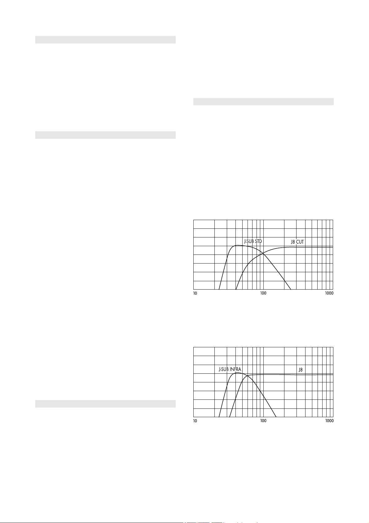
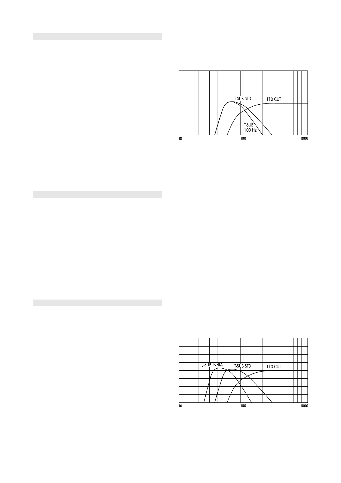
When used with additional subwoofers, the J8/J12 system
should be operated in CUT mode to gain maximum
headroom at low frequencies.
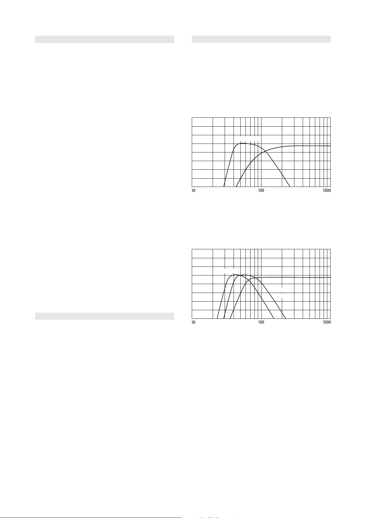
J8 / J-SUB crossover setup
When maximum low end headroom is not an issue, the
J8/J12 system can also be operated in standard mode (full
range, i.e. CUT not selected) and additional J-SUB cabinets
in INFRA mode can be used to extend the system
bandwidth down to 32 Hz.
2.1 Number of cabinets required
The number of J-Series loudspeakers to be used in an
application depends on the desired level, the distances and
the directivity requirements in the particular venue. Using the
J8 / J-SUB crossover setup, full range
d&b ArrayCalc calculator will define whether the system is
able to fulfill the requirements.
Depending on the program material and the desired level,
additional J-SUBs will be necessary to extend the system
bandwidth and headroom. In most applications a J-SUB to
J8/J12 ratio of 1:2 is sufficient. Distributed SUB arrays may
TI 385 (6.0 EN) d&b Line array design, ArrayCalc V8.x Page 4 of 54
Page 5
2.2.1 J-SUB ground stacks
Using J-SUB cabinets in L/R ground stacks provides
maximum system efficiency due to the ground coupling of
the cabinets.
2.2.2 J-SUBs flown on top of a J8/J12 array
Flown J-SUBs create a more even level distribution over
distance. Compared to a ground stacked setup the area at
the very front below the arrays has much less low frequency
level because of the longer distance to the subwoofers.
However, when a high level of low frequency energy at the
front is desired, e.g. to compensate for a loud stage level,
additional ground stacked subwoofers may be necessary.
2.2.3 Flown J-SUB columns
When complete columns of J-SUBs are flown, the increased
vertical directivity adds to the distance effect described
above and thus creates a longer throw of low frequencies.
Clever positioning of flown subwoofer columns behind the
main and outfill arrays of TOP loudspeakers can greatly
enhance both visual appearance and acoustic performance
of the complete system through increased overall coherence
between the different parts of the system.
2.3.1 Combined J-INFRA/J-SUB ground stacks
Maximum coupling and coherence of the systems are
achieved when J-INFRA and J-SUB systems are stacked
close to each other. However, make sure to keep a
minimum distance of 60 cm (2 ft) between adjacent stacks.
J-INFRA cabinets should be operated in standard mode.
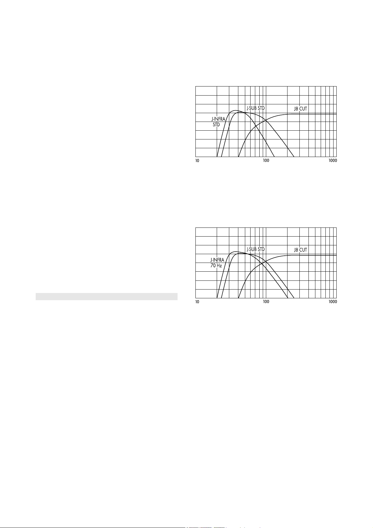
J8 / J-SUB / J-INFRA crossover setup
2.3.2 Flown J-SUBs, J-INFRA ground stacks
Flown columns of J-SUBs provide a higher vertical directivity
and thus a longer throw. Coupling with ground stacked
J-INFRAs will be less coherent and therefore requires the
70 Hz setting on the J-INFRA controllers.
2.2.4 J-SUB horizontal SUB array
Arranging J-SUBs in a horizontal array (SUB array)
provides the most even horizontal coverage eliminating the
cancellation zones to the left and right of the center of a
typical L/R setup. Refer to section 10.10 on page 32.
2.3 J-SUB/J-INFRA subwoofer setup
When used with J-INFRA cabinets J-SUB subwoofers are
always operated in standard mode (i.e. INFRA not
selected).
Depending on the application and the space requirements
a combination of J-SUB and J-INFRA cabinets can be set up
in several different ways.
J8 / J-SUB / J-INFRA 70 Hz crossover setup
2.3.3 Flown J-SUBs, J-INFRA SUB array
As an option J-INFRA cabinets can be set up in a horizontal
SUB array in front of the stage. Also in this case the 70 Hz
setting on the J-INFRA controllers is advantageous. The
correct alignment of the array dispersion and delay settings
is performed using ArrayCalc. Refer to section 10.10 on
page 32.
TI 385 (6.0 EN) d&b Line array design, ArrayCalc V8.x Page 5 of 54
Page 6
3. The V-Series line array
The V-Series consists of three different loudspeakers: the V8
and V12 loudspeakers and the V-SUB subwoofer. The V8
and V12 are mechanically and acoustically compatible
loudspeakers providing two different horizontal coverage
angles of 80° and 120°. The dispersion of both systems is
symmetrical and well controlled to frequencies down to
250 Hz, their bandwidth reaching from 65 Hz to 18 kHz.
V-Series loudspeakers can be operated with d&b D12,
D20 or D80 amplifiers. With D20 and D80 amplifiers d&b
ArrayProcessing is available.
In the vertical plane the V8 and V12 loudspeakers produce
a wavefront that allows splay angle settings ranging from
0° to 14° (1° increments). An array should consist of a
minimum of four cabinets - either V8, V12 or a combination
of both.
The V8 with its 80° horizontal dispersion and high output
capability can cover any distance range up to 100 m
(330 ft) depending on the vertical configuration of the
array and the climatic conditions.
The V12 offers a wider horizontal coverage which is
particularly useful for short and medium throw applications.
Using a combination of V8 and V12 cabinets enables the
user to create a venue specific dispersion and energy
pattern.
The V-SUB cardioid subwoofer extends the system
bandwidth down to 37 Hz while providing exceptional
dispersion control either flown or ground stacked in arrays
or set up individually.
The J-INFRA cardioid subwoofer is an optional extension to
a V8/V12/V-SUB system. It is used in ground stacked
configurations and extends the system bandwidth down to
27 Hz while adding impressive low frequency headroom.
3.2 V-SUB subwoofer setup
V-SUB cabinets can be used ground stacked, as a
horizontal SUB array or integrated into the flown array,
either on top of a V8/V12 array or flown as a separate
column.
The V-SUB cabinet offers a cardioid dispersion pattern
throughout its entire operating bandwidth.
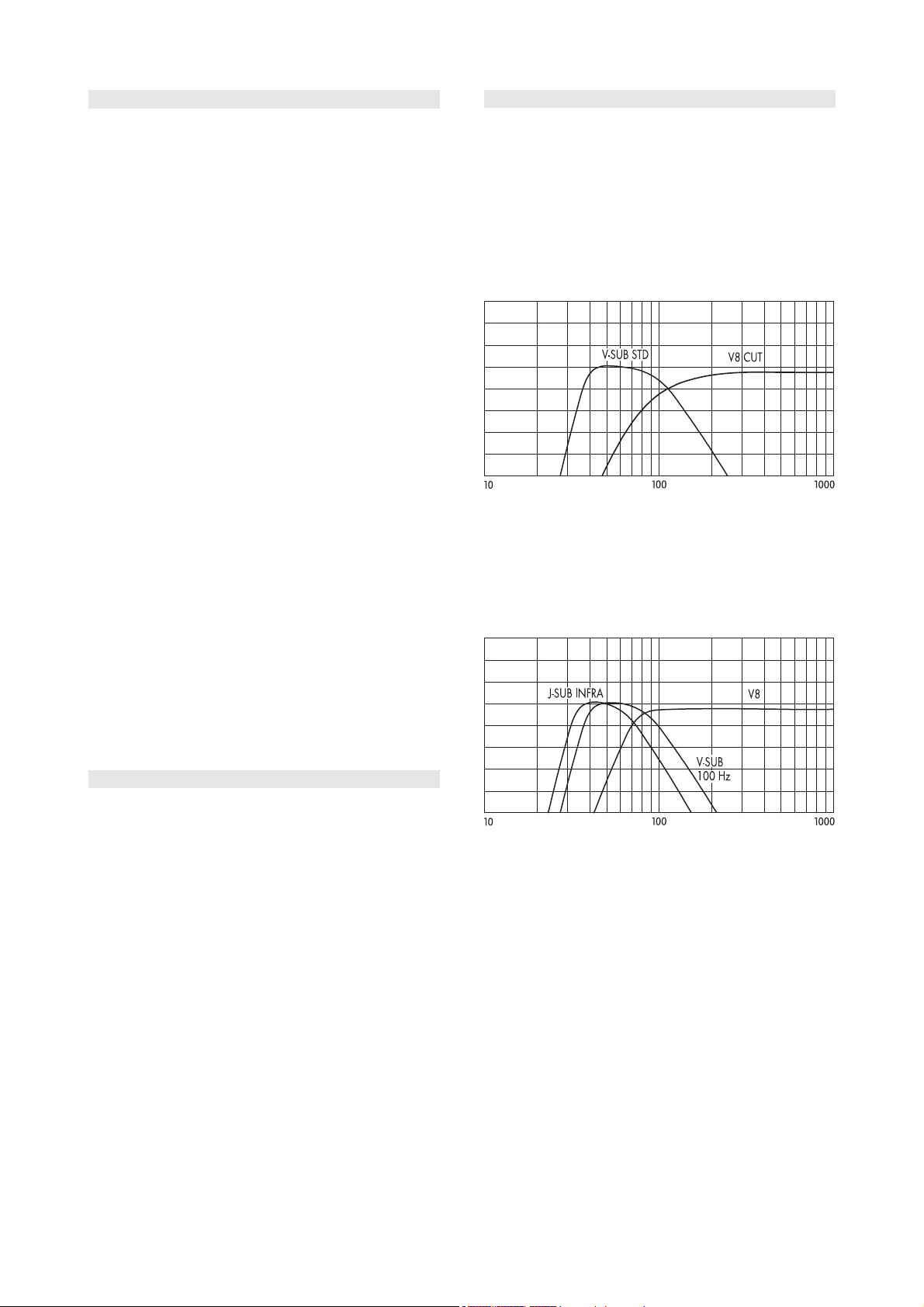
When used with additional subwoofers, the V8/V12 system
should be operated in CUT mode to gain maximum
headroom at low frequencies.
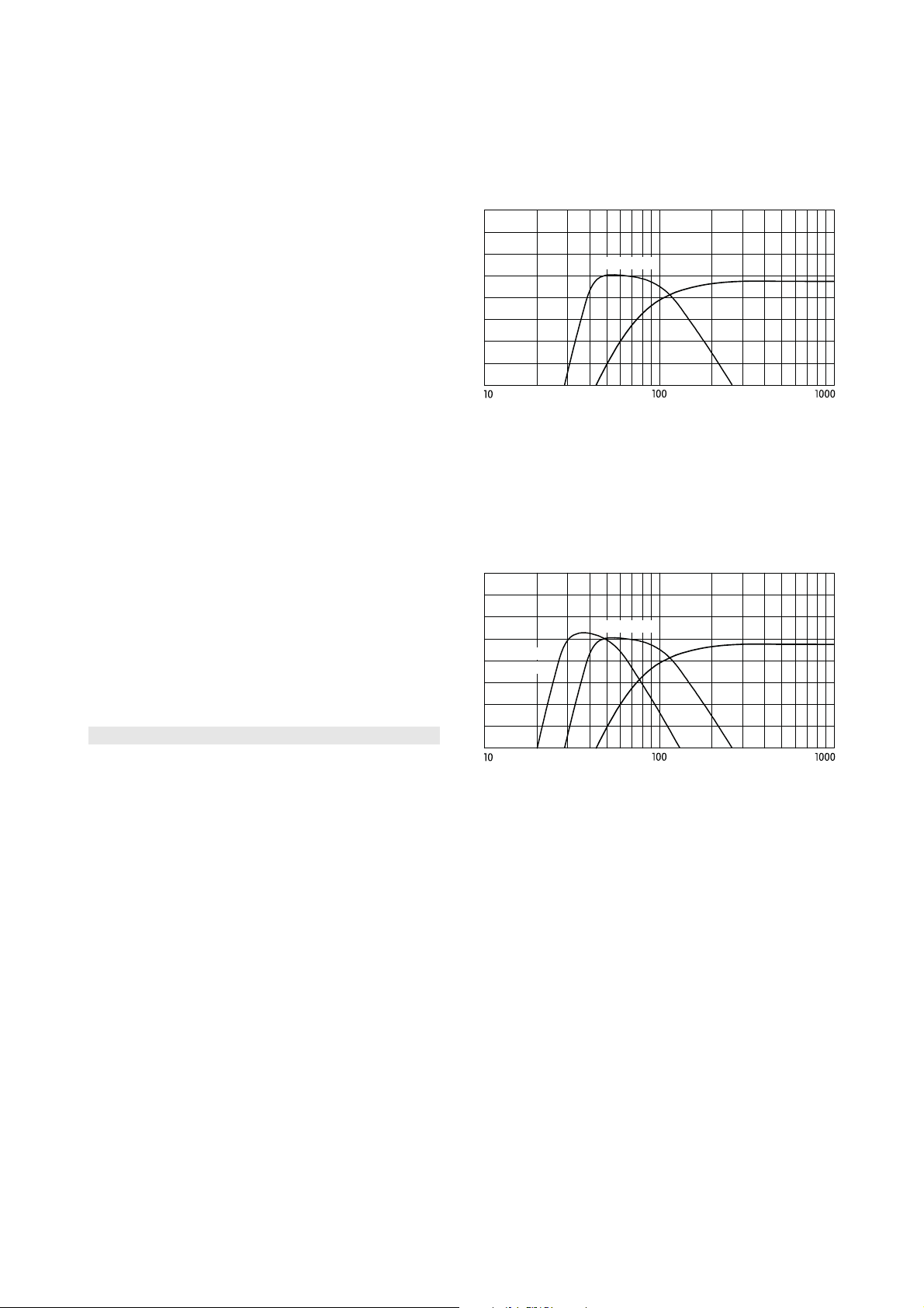
V8 / V-SUB crossover setup
When maximum low end headroom is not an issue, the V8/
V12 system can also be operated in standard mode (full
range, i.e. CUT not selected) and additional V-SUB cabinets
in 100 Hz mode or J-SUB cabinets in INFRA mode can be
used to extend the system bandwidth down to
38 Hz/32 Hz.
3.1 Number of cabinets required
The number of V-Series loudspeakers to be used in an
application depends on the desired level, the distances and
the directivity requirements in the particular venue. Using the
d&b ArrayCalc calculator will define whether the system is
able to fulfill the requirements.
Depending on the program material and the desired level,
additional V-SUBs will be necessary to extend the system
bandwidth and headroom. In most applications a V-SUB to
V8/V12 ratio of 1:2 is sufficient. Distributed SUB arrays
may require a higher number of subwoofers, such as a
V-SUB to V8/V12 ratio of 2:3.
When additional J-INFRA systems are used, one cabinet
provides the very low frequency extension for two V-SUB
subwoofers, thus generally reducing the total number of
V-SUBs required.
V8 / V-SUB / J-SUB crossover setup, full range
TI 385 (6.0 EN) d&b Line array design, ArrayCalc V8.x Page 6 of 54
Page 7
3.2.1 V-SUB ground stacks
Using V-SUB cabinets in L/R ground stacks provides
maximum system efficiency due to the ground coupling of
the cabinets.
3.2.2 V-SUBs flown on top of a V8/V12 array
Flown V-SUBs create a more even level distribution over
distance. Compared to a ground stacked setup the area at
the very front below the arrays has much less low frequency
level because of the longer distance to the subwoofers.
However, when a high level of low frequency energy at the
front is desired, e.g. to compensate for a loud stage level,
additional ground stacked subwoofers may be necessary.
3.2.3 Flown V-SUB columns
When complete columns of V-SUBs are flown, the increased
vertical directivity adds to the distance effect described
above and thus creates a longer throw of low frequencies.
Clever positioning of flown subwoofer columns behind the
main and outfill arrays of TOP loudspeakers can greatly
enhance both visual appearance and acoustic performance
of the complete system through increased overall coherence
between the different parts of the system. Refer to V-Series
setup example 6a on page .
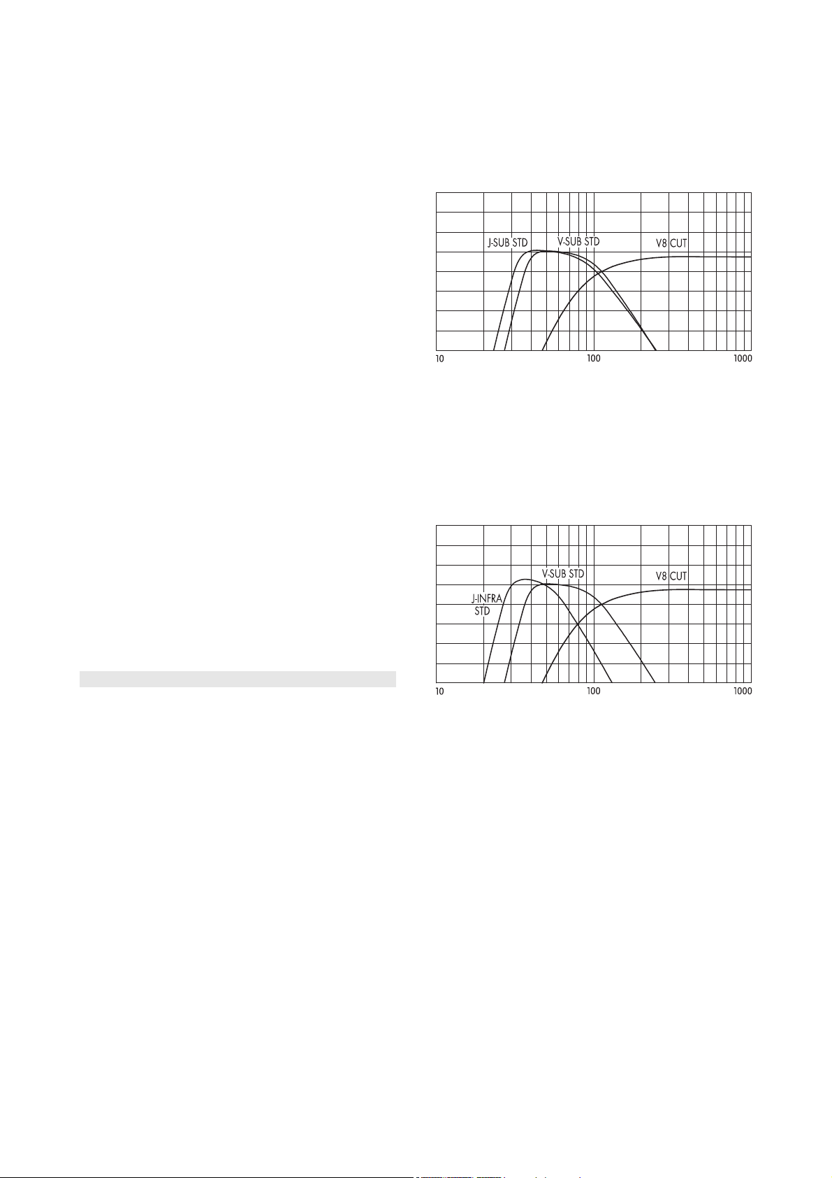
3.3.1 Combined J-, V-SUB ground stacks
Maximum coupling and coherence of the systems are
achieved when J-SUB and V-SUB systems are stacked close
to each other. However, make sure to keep a minimum
distance of 60 cm (2 ft) between adjacent stacks. J-SUB
cabinets should be operated in standard mode.
V8 / V-SUB / J-SUB crossover setup
3.3.2 Flown V-, J-SUBs or J-INFRA ground stacks
Flown columns of V-SUBs provide a higher vertical
directivity and thus a longer throw. Ground stacked J-SUBs
or J-INFRA can be operated in either crossover mode
depending on the ratio of flown to ground stacked
subwoofers.
3.2.4 V-SUB horizontal SUB array
Arranging V-SUBs in a horizontal array (SUB array)
provides the most even horizontal coverage eliminating the
cancellation zones to the left and right of the center of a
typical L/R setup. Refer to section 10.10 on page 32.
3.3 V-, J-SUB/J-INFRA subwoofer setup
When used with J-SUB and J-INFRA cabinets, V-SUB
subwoofers are always operated in standard mode (i.e.
100 Hz not selected).
Depending on the application and the space requirements
a combination of V-SUB and J-SUB / J-INFRA cabinets
can be set up in several different ways.
V8 / V-SUB / J-INFRA crossover setup
3.3.3 Flown V-SUBs, J-INFRA SUB array
As an option J-INFRA cabinets can be set up in a horizontal
SUB array in front of the stage. In this case the 70 Hz
setting on the J-INFRA controllers is advantageous. The
correct alignment of the array dispersion and delay settings
is performed using ArrayCalc. Refer to section 10.10 on
page 32.
TI 385 (6.0 EN) d&b Line array design, ArrayCalc V8.x Page 7 of 54
Page 8
4. The Y-Series line array
Y-SUB STD
Y8 CUT
Y8
J-SUB INFRA
Y-SUB
100 Hz
The Y-Series line array consists of three different
loudspeakers: the Y8 and Y12 loudspeakers and the Y-SUB
subwoofer. The Y8 and Y12 are mechanically and
acoustically compatible loudspeakers providing two
different horizontal coverage angles of 80° and 120°. The
dispersion of both systems is symmetrical and well
controlled to frequencies down to 500 Hz, their bandwidth
reaching from 54 Hz to 19 kHz.
Y-Series loudspeakers can be operated with d&b D6, D12,
D20 or D80 amplifiers. With D20 and D80 amplifiers d&b
ArrayProcessing is available.
In the vertical plane the Y8 and Y12 loudspeakers produce
a wavefront that allows splay angle settings ranging from
0° to 14° (1° increments). An array should consist of a
minimum of four cabinets - either Y8, Y12 or a combination
of both.
The Y8 with its 80° horizontal dispersion and high output
capability can cover any distance range up to 100 m
(330 ft) depending on the vertical configuration of the
array and the climatic conditions.
The Y12 offers a wider horizontal coverage which is
particularly useful for short and medium throw applications.
Using a combination of Y8 and Y12 cabinets enables the
user to create a venue specific dispersion and energy
pattern.
The Y-SUB cardioid subwoofer extends the system
bandwidth down to 39 Hz while providing exceptional
dispersion control either flown or ground stacked in arrays
or set up individually.
The J-INFRA cardioid subwoofer is an optional extension to
a Y8/Y12/Y-SUB system. It is used in ground stacked
configurations and extends the system bandwidth down to
27 Hz while adding impressive low frequency headroom.
4.2 Y-SUB subwoofer setup
Y-SUB cabinets can be used ground stacked, as a
horizontal SUB array or integrated into the flown array,
either on top of a Y8/Y12 array or flown as a separate
column.
The Y-SUB cabinet offers a cardioid dispersion pattern
throughout its entire operating bandwidth.
When used with additional subwoofers, the Y8/Y12 system
should be operated in CUT mode to gain maximum
headroom at low frequencies.
Y8 /Y-SUB crossover setup
When maximum low end headroom is not an issue, the Y8/
Y12 system can also be operated in standard mode (full
range, i.e. CUT not selected) and additional Y-SUB cabinets
in 100 Hz mode or J-SUB cabinets in INFRA mode can be
used to extend the system bandwidth down to
38 Hz/32 Hz.
4.1 Number of cabinets required
The number of Y-Series loudspeakers to be used in an
Y8 / Y-SUB / J-SUB crossover setup, full range
application depends on the desired level, the distances and
the directivity requirements in the particular venue. Using the
d&b ArrayCalc calculator will define whether the system is
able to fulfill the requirements.
Depending on the program material and the desired level,
additional Y-SUBs will be necessary to extend the system
bandwidth and headroom. In most applications a Y-SUB to
Y8/Y12 ratio of 1:2 is sufficient. Distributed SUB arrays
may require a higher number of subwoofers, such as a
Y-SUB to Y8/Y12 ratio of 2:3 or higher.
When additional J-INFRA systems are used, one cabinet
provides the very low frequency extension for up to four
Y-SUB subwoofers, thus generally reducing the total number
of Y-SUBs required.
TI 385 (6.0 EN) d&b Line array design, ArrayCalc V8.x Page 8 of 54
Page 9
4.2.1 Y-SUB ground stacks
Y-SUB STD
Y8 CUT
Y-SUB STD
Y8 CUT
J-INFRA
STD
Using Y-SUB cabinets in L/R ground stacks provides
maximum system efficiency due to the ground coupling of
the cabinets.
4.2.2 Y-SUBs flown on top of a Y8/Y12 array
Flown Y-SUBs create a more even level distribution over
distance. Compared to a ground stacked setup the area at
the very front below the arrays has much less low frequency
level because of the longer distance to the subwoofers.
However, when a high level of low frequency energy at the
front is desired, e.g. to compensate for a loud stage level,
additional ground stacked subwoofers may be necessary.
4.2.3 Flown Y-SUB columns
When complete columns of Y-SUBs are flown, the increased
vertical directivity adds to the distance effect described
above and thus creates a longer throw of low frequencies.
Clever positioning of flown subwoofer columns behind the
main and outfill arrays of TOP loudspeakers can greatly
enhance both visual appearance and acoustic performance
of the complete system through increased overall coherence
between the different parts of the system.
4.3.1 Combined J-, Y-SUB ground stacks
Maximum coupling and coherence of the systems are
achieved when J-SUB and Y-SUB systems are stacked close
to each other. However, make sure to keep a minimum
distance of 60 cm (2 ft) between adjacent stacks. J-SUB
cabinets should be operated in standard mode.
Y8 / Y-SUB / J-SUB crossover setup
4.3.2 Flown Y-, J-SUBs or J-INFRA ground stacks
Flown columns of Y-SUBs provide a higher vertical
directivity and thus a longer throw. Ground stacked J-SUBs
or J-INFRA can be operated in either crossover mode
depending on the ratio of flown to ground stacked
subwoofers.
4.2.4 Y-SUB horizontal SUB array
Arranging Y-SUBs in a horizontal array (SUB array)
provides the most even horizontal coverage eliminating the
cancellation zones to the left and right of the center of a
typical L/R setup. Refer to section 10.10 on page 32.
4.3 V-, Y-, J-SUB/J-INFRA subwoofer setup
Y-SUB and V-SUB cabinets can be combined in virtually
any application that does not require mechanical
compatibility. Their modes should always be synchronized
(i.e. both in 100 Hz mode or both in standard mode).
When used with J-SUB and J-INFRA cabinets, Y-SUB
subwoofers are always operated in standard mode (i.e.
100 Hz not selected).
Depending on the application and the space requirements
a combination of Y-SUB and J-SUB / J-INFRA cabinets can
be set up in several different ways.
Y8 / Y-SUB / J-INFRA crossover setup
4.3.3 Flown Y-SUBs, J-INFRA SUB array
As an option J-INFRA cabinets can be set up in a horizontal
SUB array in front of the stage. In this case the 70 Hz
setting on the J-INFRA controllers is advantageous. The
correct alignment of the array dispersion and delay settings
is performed using ArrayCalc. Refer to section 10.10 on
page 32.
TI 385 (6.0 EN) d&b Line array design, ArrayCalc V8.x Page 9 of 54
Page 10
5. The Q-Series line array
The Q1 is a compact and lightweight line array cabinet
providing a 75° constant directivity coverage in the
horizontal plane down to 400 Hz. The system can be used
from very small configurations of two cabinets per array up
to a maximum of twenty cabinets per array for larger
venues.
Q1 cabinets have a very low height of only 30 cm (1 ft)
and when combined in arrays its accurate wavefront covers
up to 14° vertically per cabinet, and couples coherently up
to 12 kHz when configured in a straight (0° splay) long
throw section. The Q1 covers the frequency range from
60 Hz to 17 kHz.
The Q7 and Q10 cabinets are mechanically and
acoustically compatible loudspeakers with 75° x 40° and
110° x 40° spherical dispersion patterns which can be
used as a downfill (Q7) or nearfill extension with Q1
arrays.
Smaller configurations of Q1 cabinets can also be used
ground stacked, supported by Q-SUB cabinets. The most
even energy distribution in the audience area will however
be achieved with a flown array.
The TI assumes that all Q-Series cabinets are driven by d&b
D6 or D12 amplifiers. E-PAC amplifiers do not provide HFC
and CSA settings.
When used with subwoofers, the Q1 systems should be
operated in CUT mode to gain maximum headroom at low
frequencies.
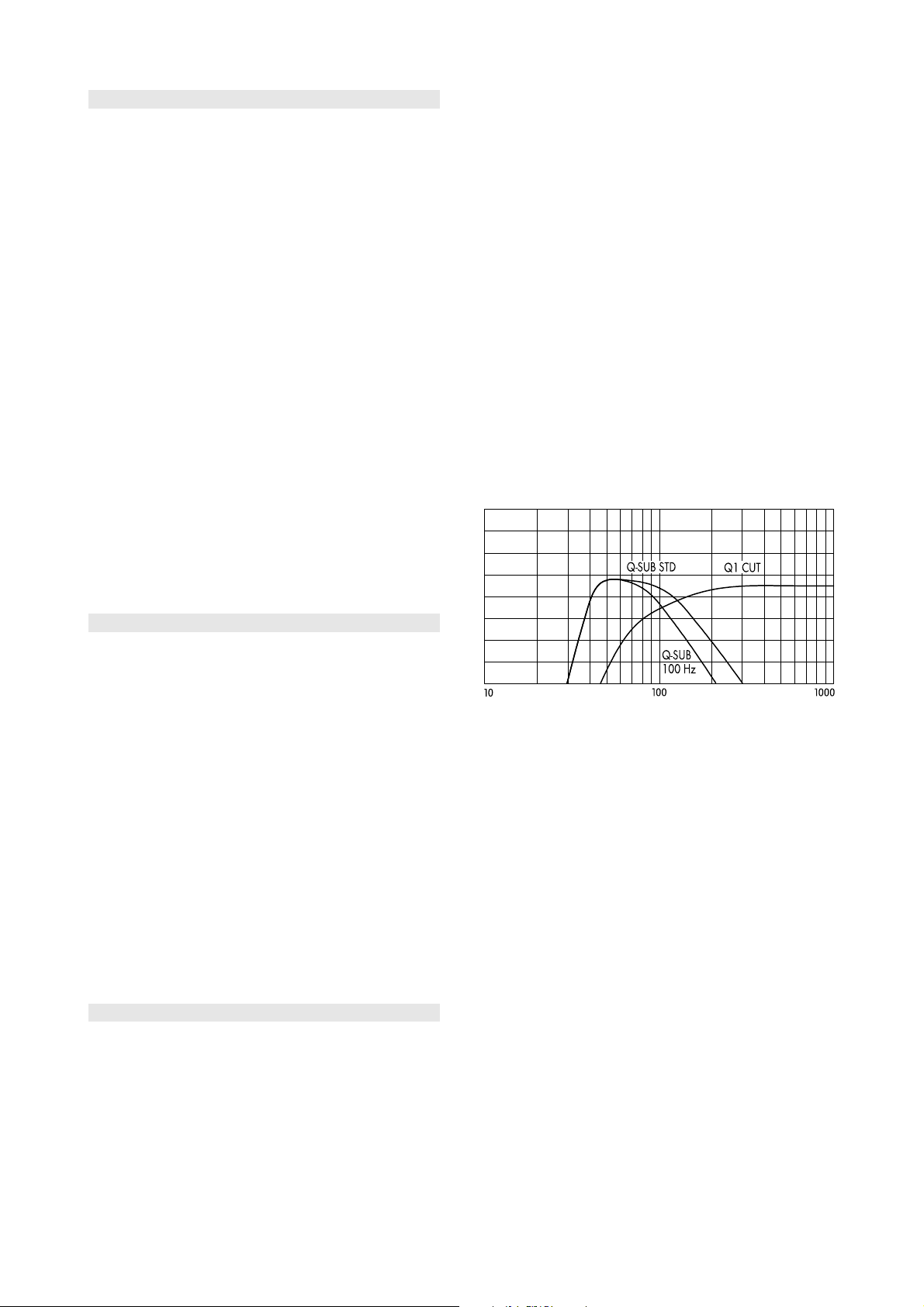
Q-SUB (40 – 100/130 Hz)
Q-SUB cabinets can be used ground stacked or integrated
into the flown array, either on top of a Q1 array or flown
as a separate column.
Flown Q-SUBs create a different level distribution in the
audience area than ground stacked ones. In particular the
area at the very front below the arrays has much less low
frequency energy when subwoofers are included in the
array. This can be very useful in applications that do not
require high levels of low frequency energy at the front,
however for an event with high stage level additional
ground stacked subwoofers may be necessary.
For Q1 arrays consisting of three or more cabinets we
recommend the use of the 100 Hz setting for the Q-SUB
systems. Smaller Q1 arrays providing less coupling at low
frequencies may benefit from the higher crossover
frequency of the standard mode of the Q-SUBs (130 Hz).
5.1 Number of cabinets required
The number of Q1 cabinets to be used in an application
depends on the desired level, the distances and the
directivity requirements in the particular venue. Using the
d&b ArrayCalc calculator will prove whether the system is
able to fulfill the requirements.
Depending on the program material and the desired level
additional Q-SUB subwoofer systems will be necessary to
extend the system bandwidth and headroom. The number
of Q-SUBs needed per Q1 cabinet for serious full-range
program will decrease with the size of the system. For small
setups a 1:1 ratio is recommended, for example four
Q-SUBs to four Q1s, while larger systems will work with a
2:3 ratio, for example eight Q-SUBs to twelve Q1s. Please
note that CSA setups require a multiple of three Q-SUB
cabinets.
As an option Q1 systems can also be used with J-SUB or
J-INFRA subwoofers.
5.2 Subwoofer setup
Subwoofers are operated most efficiently when stacked on
the ground. For cleanest sound and coverage we
recommend arranging subwoofers in a CSA configuration
as described in d&b TI 330 Cardioid SUB array which is
available for download from the d&b audiotechnik website
at www.dbaudio.com.
Q1/Q-SUB crossover setup
Compared to a standard Q-SUB configuration a CSA setup
produces slightly less level above 70 Hz, so it may be
advantageous to use the standard (130 Hz) amplifier
setting.
J-SUB (32 – 70/100 Hz)
J-SUB cabinets can be used to supplement a Q1 system in
different ways.
If the system is equipped with a sufficient number of Q-SUB
cabinets, J-SUBs can be used to extend its bandwidth to
below 32 Hz. Driven by D12 amplifiers set to INFRA mode
one J-SUB will supplement up to four Q-SUB cabinets.
This combination will achieve its maximum headroom when
the Q-SUBs are operated in the 130 Hz mode. If for audio
reasons the lower crossover frequency to the Q1s is desired
you may also reduce the gain of the Q-SUB amplifiers.
Decreasing the gain by 2.5 dB will create the same
downward shift to the upper slope as switching to the
100 Hz setting, but with less low frequency boost.
TI 385 (6.0 EN) d&b Line array design, ArrayCalc V8.x Page 10 of 54
Page 11
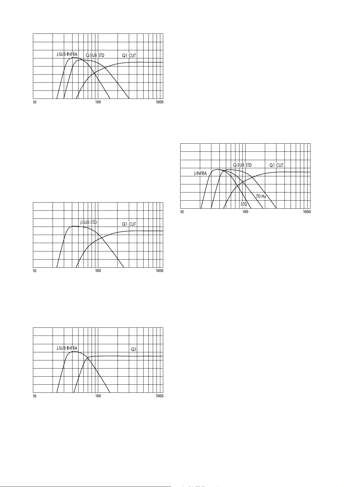
Q1/Q-SUB/J-SUB crossover setup
Please note that a combined ground stack consisting of
Q-SUB and J-SUB cabinets will only provide a consistent
directivity when Q-SUBs are used in CSA setups. Also make
sure to keep the required distance of 60 cm (2 ft) between
the stacks in order to not adversely affect the cardioid
directivity of the systems.
J-SUB subwoofers can also be used as an alternative to
ground stacked Q-SUBs. In this case J-SUB cabinets are
operated in standard mode with a crossover frequency of
100 Hz. One J-SUB will replace three Q-SUB cabinets in a
CSA setup and extends the system bandwidth down to
32 Hz.
J-INFRA (27 – 60/70 Hz)
To achieve the ultimate low frequency extension for a Q
system consisting of Q1 and Q-SUB cabinets, additional
J-INFRA subwoofers can be used. They provide a standard
(60 Hz) and a 70 Hz mode. The selection of the mode
depends on the coupling between J-INFRA and Q-SUB
cabinets in the actual setup. When combined in a ground
stack the standard (60 Hz) mode provides more headroom
at very low frequencies.
Please note that a combined ground stack consisting of
Q-SUB and J-INFRA cabinets will only provide a consistent
directivity when Q-SUBs are used in CSA setups. Also make
sure to keep the required distance of 60 cm (2 ft) between
the stacks in order not to adversely affect the cardioid
directivity of the systems.
Q1/J-SUB crossover setup
J-SUB cabinets in INFRA mode can be used to extend the
bandwidth of a Q1 line array operated in full-range mode,
without Q-SUBs. As this application does not expand the
headroom of the Q1 array it is only useful when medium
levels but very low frequencies are required, for example
for special effects.
Q1/Q-SUB/J-INFRA crossover setup
Q1/J-SUB crossover setup, full range
TI 385 (6.0 EN) d&b Line array design, ArrayCalc V8.x Page 11 of 54
Page 12
6. The T-Series line array
The T10 is a very compact loudspeaker system which can
be used both as a line array and as a high directivity point
source speaker. For these applications the T10 cabinet
provides two different dispersion characteristics which can
be swapped over without any tools.
In line array mode the T10 provides a 105° constant
directivity coverage in the horizontal plane allowing for
vertical splay angles of up to 15° per cabinet. The system
can be used from very small configurations of three
cabinets per array up to a maximum of 20 cabinets per
array for larger venues. The T10 covers the frequency
range from 68 Hz to 18 kHz.
The T-SUB subwoofer extends the system bandwidth down
to 47 Hz either flown or ground stacked.
Smaller configurations of T10 cabinets can also be used
ground stacked supported by T-SUB cabinets or mounted
on a high stand. The most even energy distribution in the
audience area will however be achieved with a flown
array.
6.1 Number of cabinets required
The number of T10 cabinets to be used in an application
depends on the desired level, the distances and the
directivity requirements in the particular venue. Using the
d&b ArrayCalc calculator will prove whether the system is
able to fulfill the requirements.
Depending on the program material and the desired level
additional T-SUB subwoofer systems will be necessary to
extend the system bandwidth and headroom. The number
of T-SUBs needed per T10 cabinet for serious full-range
program will decrease with the size of the system. For small
setups a 1:3 ratio is recommended, for example one T-SUB
to three T10s.
For T10 arrays consisting of three or more cabinets we
recommend the use of the 100 Hz setting for the T-SUB
systems. Smaller T10 arrays providing less coupling at low
frequencies may benefit from the higher crossover
frequency of the standard mode of the T-SUB (140 Hz).
T10 / T-SUB crossover setup
B4-SUB (40 – 100/150 Hz)
Q-SUB (40 – 100/130 Hz)
E15X-SUB (37 – 100/140 Hz)
As an option T10 systems can also be used with B4-SUB,
Q-SUB or E15X-SUB subwoofers. These cabinets cannot be
integrated into a flown T-Series rig. However, they allow the
deployment of T10 cabinets on their M20 flanges using
either the T-Series Base Plate or the T-Series Cluster Bracket.
The T-Series Base Plate connects directly to the M20 flange
and supports an array of up to 6 x T10 cabinets while the
T-Series Cluster Bracket is pole mounted on the M20 flange
and supports up to three T10 cabinets.
To achieve the best acoustic results in critical venues, we
recommend to use the B4-SUB. It is a compact and effective
solution providing a cardioid dispersion from a single
amplifier channel.
Like the T-SUB these systems provide a 100 Hz circuit on
their controller which can be set accordingly.
6.2 Subwoofer setup
When used with subwoofers, the T10 systems should be
operated in CUT mode to gain maximum headroom at low
frequencies.
J-SUB (32 – 70/100 Hz)
J-SUB cabinets in INFRA mode can be used to extend the
frequency range of a T-Series system. To gain maximum
headroom T-SUBs should be operated in standard mode
(i.e. 100 Hz not selected).
T-SUB (47 – 100/140 Hz)
T-SUB cabinets can be used to supplement the LF headroom
of the T10 loudspeakers in various combinations. They can
be used ground stacked or integrated into the flown array,
either on top of a T10 array or flown as a separate column.
Flown T-SUBs create a different level distribution in the
audience area than ground stacked ones. In particular the
area at the very front below the arrays has much less low
frequency energy when subwoofers are included in the
array.
T10 / T-SUB / J-SUB crossover setup
This can be very useful in applications that do not require
high levels of low frequency energy at the front, however
for an event requiring a loud stage level additional ground
stacked subwoofers may be necessary.
TI 385 (6.0 EN) d&b Line array design, ArrayCalc V8.x Page 12 of 54
Page 13
7. The xA-Series line array
The 10AL and 10AL-D line array modules of the xA-Series
have been specifically designed for fixed installations with
visually unobtrusive integrated rigging systems.
For these applications, the cabinets are available with two
different constant directivity dispersion characteristics in the
horizontal plane:
The 10AL provides a 75° coverage while the 10AL-D
version provides 105° of coverage. In the coupling plane,
both allow for vertical splay angles of up to 15° per
cabinet. Both versions may be combined in one array, for
example with 10AL cabinets at the top for longer distances
and one or two 10AL-D to cover the areas near the stage.
Both systems can be used from small configurations of three
cabinets per array up to a maximum of 9 cabinets per
array.
The 10AL (-D) covers the frequency range from 60 Hz to
18 kHz. 18A-SUB or 27A-SUB subwoofers extend the
system bandwidth down to 37 Hz or 40 Hz, respectively.
They can be flown in a separate column, integrated at the
top or within an array or used as ground stacked
applications. When they are flown together with line array
modules, the maximum number of total cabinets is reduced
due to the additional weight.
Configurations of up to six 10AL / 10AL-D cabinets can
also be used ground stacked, supported by 18S-SUB or
27S-SUB cabinets. The most even energy distribution in the
audience area will however be achieved with a flown
array.
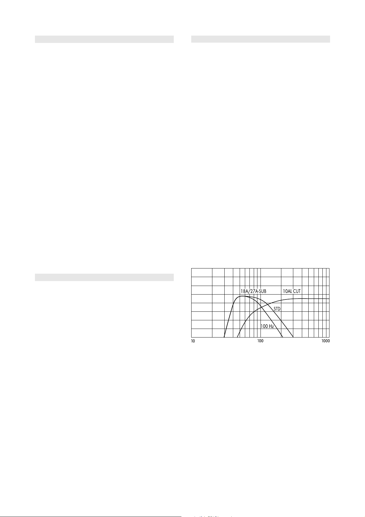
7.2 Subwoofer setup
When used with subwoofers, the 10AL(-D) systems should
be operated in CUT mode to gain maximum headroom at
low frequencies.
27A-SUB/27S-SUB (40 – 100/140 Hz)
Subwoofers can be used to supplement the LF headroom of
the 10AL loudspeakers in various combinations.
To achieve the best acoustic result in critical venues, we
recommend the use of 27A-SUB or 27S-SUB subwoofers.
They offer a compact and effective solution by providing
cardioid dispersion from a single amplifier channel.
They can be used ground stacked (27S-SUB and 27A-SUB)
or integrated into the flown array (27A-SUB), either at the
top or within a 10AL array, or flown as a separate column.
Flown subwoofers create a different level distribution in the
audience area than ground stacked ones. Particularly the
area directly at the front below the arrays provides less low
frequency energy when subwoofers are included in the
array.
This can be very useful in applications that do not require
high levels of low frequency energy at the front, however
for an event requiring a loud stage level, additional ground
stacked subwoofers may be necessary.
For 10AL arrays consisting of three or more cabinets, we
recommend the use of the 100 Hz setting for the
subwoofers. Smaller 10AL arrays providing less coupling at
low frequencies may benefit from the higher crossover
frequency of the standard mode (140 Hz).
7.1 Number of cabinets required
The number of 10AL or 10AL-D cabinets to be used in one
application depends on the desired level, the distances to
be covered and the directivity requirements of the particular
venue. Using the d&b ArrayCalc calculator will prove
whether the system is able to fulfill the requirements.
Depending on the program material and the desired level
additional 18A-SUB or 27A-SUB subwoofer systems may
be necessary to extend the system bandwidth and
headroom. The number of subwoofers required per 10AL
(-D) cabinet to provide a serious full-range program
decreases with the size of the system. For small to medium
size setups, a 1:3 ratio is recommended, for example one
27A-SUB to three 10ALs.
10AL / 18A/27A-SUB crossover setup
18A-SUB/18S-SUB (37 – 100/140 Hz)
18A-SUB or 18S-SUB cabinets can be used in the same
way as 27A-SUB or 27S-SUB cabinets but without the
benefit of cardioid dispersion.
For these systems, just like for the 27S/A-SUBs, a 100 Hz
circuit is available on the controller, which can be set
accordingly.
TI 385 (6.0 EN) d&b Line array design, ArrayCalc V8.x Page 13 of 54
Page 14

8. The d&b point sources
From Version V7x.x, a range of d&b point source
loudspeakers is available for integration into a project. All
current top cabinets of the E-Series, Y(i)P-Series, Q(i)7,
Q(i)10, T(i)10PS and xS-Series can be selected, both in
stand-alone projects and in combination with line arrays.
Please note that a T(i)10L loudspeaker that is deployed
horizontally may also be used as a single nearfill with the
T10PS setup although its polar dispersion does not reflect a
"point source".
For cabinets that are equipped with rotatable HF horns,
both horn orientations can be selected separately. Each
selectable orientation for a specific loudspeaker type uses
its own measured polar data set. This is defined by the
chosen nominal horizontal and vertical dispersion angles
and follows the convention [SystemName] [horizontal
dispersion] x [vertical dispersion] while the cabinet itself
remains in its typical mechanical orientation, i.e. in an
upright position (e.g. 10S 75x50; E6 55x100; Q7 40x75
etc).
If a system is used lying on its side, the standard dataset
must be used and the cabinet rotation must be set to either
90°(on its left side, seen from a listener's position) or 270°
(on its right side, seen from a listener's position). The cabinet
can be rotated in steps of 90° degrees. Each individual
cabinet can be freely positioned within the room with
horizontal or vertical aiming.
Selecting a loudspeaker optionally displays a balloon polar
plot or its vertical aiming into the room.
More specific loudspeaker data can be found in the
relevant documentation of the respective d&b products.
9. Column loudspeakers
The xC-Series column loudspeakers are passive 2-way
designs with a passive bandpass system providing a
cardioid dispersion control with an 18 dB average
broadband attenuation to the rear of the loudspeakers.
The 16C behaves as a standard point source cabinet with
a 90° x 40° (h x v) dispersion and is treated accordingly
in ArrayCalc. Its HF horn orientation is fixed, as a result
there is one single set of data available. You can, of course,
change the orientation of the cabinet itself like with all point
sources.
The 24C provides a special 90° x 20° pattern with a
variable vertical aiming to produce an even level
distribution over a typical audience area. This is achieved
by adjusting the vertical angle of the complete HF array
between 0° and –14°combined with a 5° down tilt to the
dispersion of low and mid frequencies.
When the 24C-E Cardioid column extender is attached,
vertical dispersion control is extended towards low
frequencies by another full octave.
8.1 Number of cabinets required
The number of point source cabinets is primarily defined by
their specific application, for example as nearfill or delay
systems or as the main system. Of course, the number of
cabinets also depends on the desired level, the distances to
be covered and the directivity requirements in the particular
venue or project. Using the d&b ArrayCalc calculator will
prove whether the system is able to fulfill the specific
requirements.
Depending on the program material and the desired level,
additional d&b subwoofer systems may be necessary to
extend the bandwidth and headroom
When used with subwoofers, the point sources should be
operated in CUT mode to gain maximum headroom at low
frequencies.
TI 385 (6.0 EN) d&b Line array design, ArrayCalc V8.x Page 14 of 54
Page 15

10. ArrayCalc
For both acoustic and safety reasons all d&b line arrays
must be designed using the d&b ArrayCalc simulation tool.
ArrayCalc also provides functionality to integrate individual
d&b point source loudspeakers into a simulation project.
ArrayCalc is available for PC and MAC.
ArrayCalc uses a sophisticated mathematical model
synthesizing each line-array cabinet's wavefront using
measured high-resolution dispersion data. Sound pressure
level is calculated in 3D using complex data (vector
summation).
Point sources are modelled using complex measured highresolution 3D polar data.
ArrayCalc provides the following features:
— Editing of three-dimensional listening planes to create
audience areas in a given venue and shape.
— Help function to obtain venue dimensions using laser
distance finders and inclinometers.
— Level distribution on up to five different audience areas
displayed in 3D format for selectable frequency bands
from 32 Hz to 12.5 kHz.
— Calculation of absolute sound pressure levels in
audience areas including system headroom supervision
for different input signals.
— Combination of up to 14 different array pairs distributed
across the venue plus ground stacked subwoofers in L/R
combinations or arranged as SUB array.
— Calculation of ArrayProcessing settings for line arrays
— Flown subwoofers integrated into the line arrays or flown
as separate columns.
— Additional integration of up to six groups of d&b point
source loudspeakers.
— Additional integration of xC column loudspeakers.
— Auto tuning algorithms for vertical aiming and splay
angles of arrays as well as SUB array settings.
— Tuning of all relevant amplifier settings like level, array
coupling, crossover and cardioid modes.
— Simulation of air absorption effects depending on
environmental conditions, tuning of the respective
amplifier settings.
— System time alignment between different sources and
subwoofers using impulse and phase response data.
— Calculation of load and space requirements for rigging
points.
— Calculation and supervision of electronic and physical
load conditions as well as mechanical forces within
arrays.
— Design and calculation printouts, printable parts lists for
inventory control and loading as well as DXF and EASE
export functions.
— Project file export into the d&b R1 Remote control
software.
System requirements
— PC with Intel/AMD (1 GHz or more); Windows 7 or
higher.
— or Macintosh (Intel); Mac OS 10.6 or higher.
— 2 GB RAM, 4 GB recommended.
— 100 MB of available hard disk capacity.
— Mouse, preferably with wheel.
— Minimum screen resolution 1280 x 1024; on smaller
screens viewport has to be scrolled.
10.1 ArrayCalc installation
Windows systems:
To install ArrayCalc, start ArrayCalcSetup.exe or
ArrayCalcSetup.msi and follow the instructions in the setup
dialog.
The default installation path is:
C:\Program files\dbaudio\ArrayCalc
A default project directory will be created:
Windows Version 7 or higher:
C:\Users\'username'\My Documents\dbaudio
To remove ArrayCalc from your system, go to Start –
Settings – Control Panel – Add or remove programs in the
Control Panel folder.
Select the ArrayCalc entry from the list and click the
Remove button. The uninstall routine starts and the software
is removed including all related components.
Macintosh systems:
Double-click ArrayCalc.dmg and drag ArrayCalc to your
applications folder.
To remove ArrayCalc from your system, move ArrayCalc
into the trash bin.
10.2 Starting ArrayCalc
Windows:
ArrayCalc can either be started via the Windows Start
Menu, where it will appear in Programs – dbaudio –
ArrayCalc – ArrayCalc or by double-clicking the ArrayCalc
desktop icon.
Windows automatically links ArrayCalc project files
(*.dbac2) to ArrayCalc. Alternatively, the program can
therefore be started by double-clicking on any ArrayCalc
project file.
Macintosh:
Click ArrayCalc or any ArrayCalc project file.
TI 385 (6.0 EN) d&b Line array design, ArrayCalc V8.x Page 15 of 54
Page 16

10.3 ArrayCalc menu options and Toolbar
The drop-down menus "File", "View", "Sources","Extras" and
"Help" on top of the page provide access to additional
functions of ArrayCalc. Several menu items can also be
accessed directly by clicking the respective button in the
toolbar underneath.
10.3.1 File menu
— New: Creates a new project by loading the default
project. Modifying a simple existing setup is usually
much faster than starting without any data.
— Open / Save / Save as: Loads or saves the project
data including room data, arrays, SUB array design and
alignment settings from/to a file. (file format: *.dbac2).
It is possible to open setup files created with ArrayCalc
version 5.x, however additional data has to be provided
manually. Opening setups from earlier Microsoft Excel
based versions of ArrayCalc is not possible.
Note:
When saving an ArrayCalc project, all relevant
information for the related R1 Remote control
project such as amplifiers, groups and control
elements is generated and saved to the same file.
To operate the simulated ArrayCalc project in R1,
just open the respective *dbac2 file.
— Open recent project: Provides direct access to the
last six projects saved.
— Open example project: Provides direct access to
the example project files included in the installation
package.
— Export DXF: Exports all / the currently selected array
or the SUB array to a *.dxf graphics file. The units used
in the dxf-file are millimeters. However for compatibility
reasons the unit formatting in the dxf-file is omitted, hence
several CAD systems import the data as "unitless".
— Export EASE: Exports the selected array to a file which
can be imported by the d&b Line Array GLL or DLL for
EASE 4.x.
— Export PNG: Only available from the 3D plot page;
exports the 3D plot, the color scale and the underlying
signal selection to a *.png file.
— Print: Print options for several pages of ArrayCalc.
— Print preview: Provides access to a print preview with
several options (depending on the printer selected).
— New instance: Opens another instance of ArrayCalc.
— Exit: Closes ArrayCalc.
10.3.2 View menu
— Toolbar: Allows the toolbar to be switched on/off.
— Status bar: Allows the status bar to be switched
on/off.
10.3.3 Sources menu
When working on the Sources page, the Sources menu
provides the following functions:
— Add array: Adds a new empty array to the project.
The maximum number of arrays is fourteen.
— Auto splay: Provides starting values for the splay
angles of the selected array.
— Add point sources: Adds a new empty point sources
dialog to the project. The maximum number of point
source groups is fourteen. Each group may consist of up
to 14 single point sources. You can also select column
loudspeakers from this dialog by choosing xC-Series
from the system selection.
— Rename: Highlights the name of the selected source
for editing.
— Copy: Creates a copy of the selected source settings in
the internal clipboard.
— Paste: Pastes all source settings copied to the internal
clipboard into the selected source.
— Paste as new: Creates a new source containing all
settings from the internal clipboard.
— Delete: Deletes the selected source from the project
after confirmation.
— Export source: Exports the settings of the selected
source to an ArrayCalc description file (*.dbea for
arrays, *.dbep for groups of point sources, *.dbesa for
SUB arrays).
— Import source: Imports the settings of a source from
an ArrayCalc description file (*.dbea for arrays, *.dbep
for groups of point sources, *.dbesa for SUB arrays) to
the selected source.
10.3.4 Extras / Options menu
— Units: Provides access to the selection of:
the measurement units: metric (m/kg) or imperial (ft/lbs).
the temperature units: degrees centigrade (° C) or
Fahrenheit (° F).
— Web search: Provides access to automatic update
options.
— Graphics: Provides optional color palette for bright
environment.
— R1 project: Defines the start mode of the generated
R1 project.
— Air absorption: Provides access to the environmental
settings (temperature and humidity) which are primarily
relevant to calculate excessive absorption of high
frequencies in air (see also 9.6.10). For quick access to
the global Air absorption settings, an on-off switch is
available in the toolbar at any time. A shortcut to the
Extras/Options/Air absorption settings is provided there
as well to define temperature and humidity values.
10.3.5 Help menu
— F1 Help: Provides access to this document.
— Web search: Searches the web for updates.
— System info: Provides information on the computer
system.
— About: Provides information on the version of
ArrayCalc you are using.
TI 385 (6.0 EN) d&b Line array design, ArrayCalc V8.x Page 16 of 54
Page 17
10.4 ArrayCalc workspace
The workspace is sub-divided into seven pages giving
access to the various data input tables and calculation
results:
Place the mouse pointer onto these cells and turn the mouse
wheel to scroll through the possible selections for the
respective cell.
This is a fast tool to manually set splay angles.
The usual procedure is first to enter the project description
which can be accessed from the first four pages "Venue",
"Sources", Alignment" and "3D plot". Then room data is
provided in the Venue editor which is accessible on the
Venue page (see following section).
On the Sources page, you can add line arrays to the
project and design their profiles and locations depending
on the vertical dispersion requirements for each position. In
addition, or alternatively, you can define and enter a group
of d&b point sources or column loudspeakers. Furthermore
an optional SUB array can be defined and tuned here (see
also section 10.10 SUB arrays on page 32).
If you use more than one source, the Alignment page (see
section 10.11 Alignment page on page 38) helps you to
correctly time align the sources in a next step. This also
includes the SUB array alignment.
In a third step, the 3D plot page enables you to tune and
verify the detailed settings of the horizontal aiming and
relative leveling of the arrays in order to achieve the desired
level distribution.
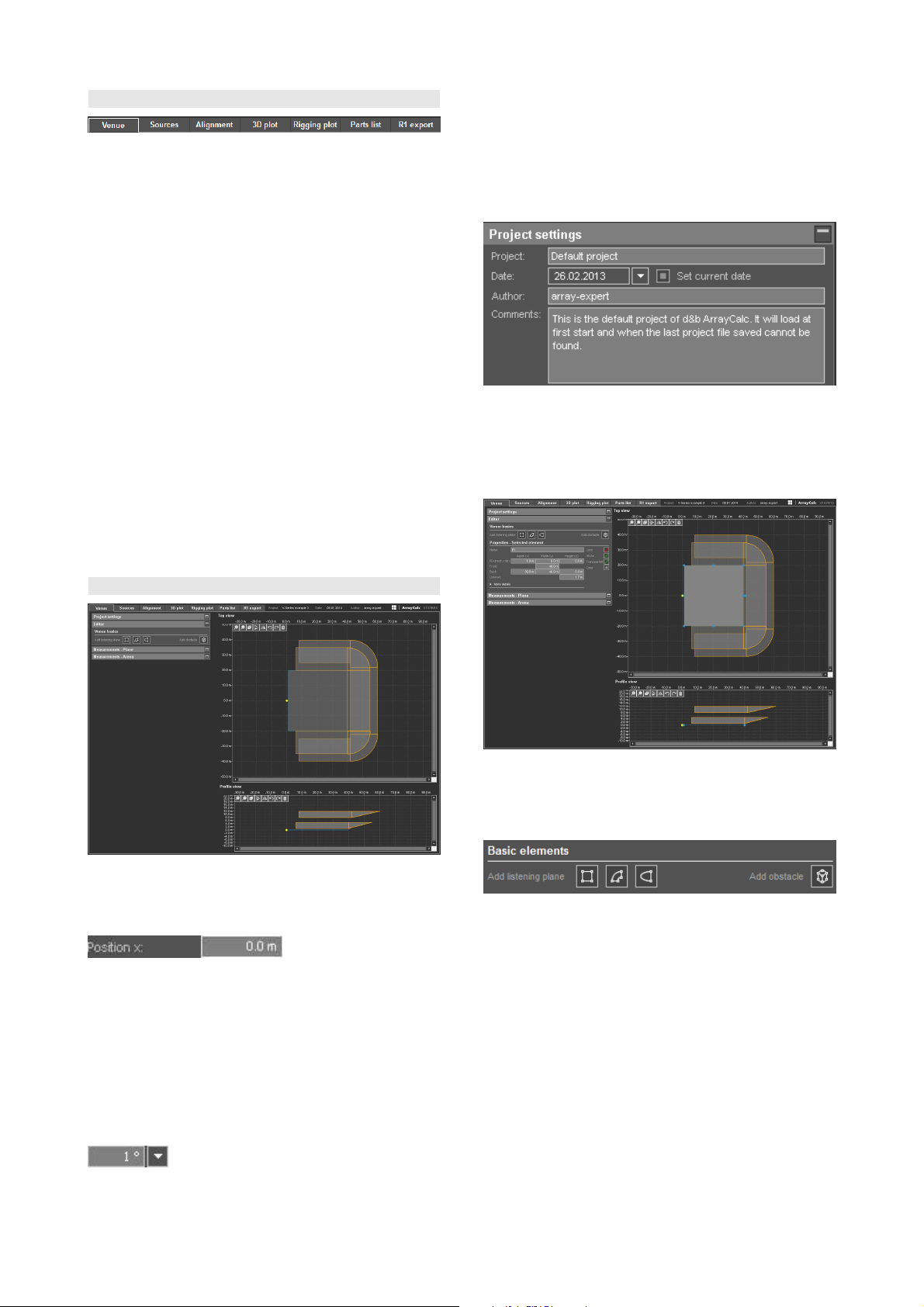
10.5 Venue page
10.5.2 Project settings
Enter information about the project you are planning. This
data will be displayed in the headline or in the dedicated
Comments sections as well as in the printouts.
10.5.3 Venue editor
10.5.1 General data input
Cells with a gray background accept direct data input.
A single click places the cursor in the cell to edit data.
A double-click additionally highlights the value left of the
decimal point for editing and replacement while a triple
click highlights the entire cell contents for editing and
replacement.
To switch between metric and imperial units, refer to section
10.3 ArrayCalc menu options on page 16.
Cells with a drop-down icon attached offer a predefined
selection of data input available from the drop-down list.
General editing
A listening plane is added to the project by clicking one of
the basic geometric shapes, the quadrangle, the arc
segment or the superelliptic plane.
A quadrangle starts as a square which can be moved,
rotated and modified to any possible shape of a
quadrangle. This is done by either modifying its coordinates
numerically or by grabbing and moving the shape with the
mouse as a whole, or dragging one of its corner points or
its rotation point in one of the diagrams.
An arc segment starts as a symmetrical section of two
concentric circle segments. It can be moved, rotated and
modified to any possible shape of an arc segment by
grabbing and dragging one of its corner points, one of its
center points or its rotation point.
In the Venue editor, an arc segment is displayed in full,
while for level calculations and mappings (3D plot) each
arc is segmented into a suitable number of quadrangles.
TI 385 (6.0 EN) d&b Line array design, ArrayCalc V8.x Page 17 of 54
Page 18

A superelliptic listening plane starts with a span of
360°and can be moved, rotated and modified to any
possible shape of an ellipse by dragging its start/end
points or by entering data into the input fields in the Venue
editor dialog.
When modifying plane coordinates, the standard shape is
symmetrical around its (front) center point. Only by using
ALT+mouse movement is the symmetry abandoned and
points can be modified individually.
Pressing the ALT key while dragging a plane activates the
Snap to element option. When this option is active, the
corner points of the plane being dragged snap to any other
corner points of the other plane to which it is dragged.
Please note that the height (z) of the snapping corner points
will be adjusted to the height (z) of the corner points of the
plane to which they are snapped.
You can select multiple listening planes and/or obstacles
for editing by pressing the CTRL (Windows) or CMD key
(OS X) while clicking the desired planes and/or obstacles
Alternatively, it is possible to select multiple listening planes
and/or obstacles by dragging a selection rectangle around
them or to select all by pressing CTRL+A (Windows) or
CMD+A (OS X).
Listening plane properties
Show: If a plane is switched off here, its borders are
displayed in dashed lines in the Venue editor. On all other
pages, the plane or its sections are not visible. It is also
excluded from all calculations.
Transparent option:
When a sound from a source hits a plane, it gets absorbed
by the plane. This is indicated by the fact that the main
beams of the relevant cabinets end as soon as they hit the
plane. Listening points on other planes without a direct line
of sight to a source or points which are in the shadow of a
particular plane do not receive any sound from the source.
This feature can be specifically helpful when simulating the
level of under balcony listening positions.
When a plane's Transparent switch is enabled, the plane
will not absorb the sound. In this case, the beams will go
"through" the plane onto any other planes that are located
in its shadow.
When the planes are set to absorbent, the system checks
every single listening point for an acoustic "sightline",
something which requires a considerable amount of
computing time. As a result, to speed up calculation,
listening planes should be switched to Transparent unless
the planes need to be absorbent to check the levels under
balconies, etc. For this reason, in every new plane the
"Transparent" option is enabled as default.
A listening plane is selected for viewing and editing its
properties by clicking the plane in one of the diagrams:
Name: Each plane can be named individually.
Plane coordinates: In the upper section, a simplified plane
definition based on symmetry of the plane itself is possible.
Listener height: Enter the typical height of the listener's ear.
In the More details section below, the three-dimensional
coordinates of each corner point can be accessed
individually. Place the cursor in one of the data input cells
(x,y,z) of a specific point to highlight the respective point in
both the Top view and the Side view diagrams.
Lock: This function protects all dimensional parameters of a
listening plane against editing. Only the name and color of
the listening plane can still be edited when the plane has
been locked.
Color: The color of each listening plane with its associated
data such as calculated levels can be defined individually.
Obstacles
A virtually unlimited number of obstacles (screens, displays,
etc.) can be defined. An obstacle is added to the project by
clicking the Obstacle button.
Name: Each obstacle can be named individually
Coordinates: The reference point for all coordinate inputs
is always the geometric center of its base edge (P4-P1; the
one opposite to the grab point). The center of the obstacle's
base edge P4-P1 is defined in the row "Origin". Its
extension in x/y/z is defined in the row "Dimensions". An
obstacle can only be symmetrical. x, y and z have to be
positive values, so it always extends upwards from its base
plane.
TI 385 (6.0 EN) d&b Line array design, ArrayCalc V8.x Page 18 of 54
Page 19

Lock/Show/Transparent/Color: Obstacles show the
same behavior as described above for the listening planes.
Obstacles are shown in the Venue editor, the Top view
diagram and in the 3D plot.
All elements
This section lists all listening planes and obstacles defined
for the current venue. You can select one or more listening
planes or obstacles from the list to edit them, either directly
in the list or using the Selected element section above. The
switches and buttons included in the first line named 'All'
affect all listening planes and obstacles defined for the
current venue.
For each plane profile to be determined, enter the distance
and the viewing angle to the closest point (Front) and the
farthest point (Back) of the plane.
From this, the x positions and heights are calculated
.
Create plane: After entering all measurements, click Create
plane to add a new listening plane.
Note: If, with very small angles (low elevation), the
measurement accuracy is not satisfactory, move the
instrument closer to the object to increase the viewing
angle. The sheet allows to input the instrument x-position
and height for each plane.
Measurements - Arena
An additional dialog which supports the input of measuring
data of general superelliptic venues, such as arenas or
stadiums using a laser inclinometer and a range finder.
Note: When multiple elements are selected
(highlighted in yellow), the changes you apply to one
element will affect all selected elements.
Export/import of venue settings
You can export defined venue settings to an ArrayCalc
venue file (*.dbacv). This file including the exported venue
settings can then be imported in other projects or in the
same project again, for example for comparative purposes.
To use the venue export/import function, select 'Export' or
'Import' from the File menu while the 'Venue' page is active.
Measurements - Plane
An additional dialog which supports the input of plane
coordinates using a laser inclinometer and a range finder.
This is a particularly useful method when the elevation of
balconies or stands has to be determined.
When you click into an entry field, the interactive 'How to'
diagram shows to which parameter this particular field
refers.
When measuring a venue with two or more tiers, enter the
data for each tier separately by measuring its lower and
upper edges. After that, click Create planes. Then repeat
the procedure for the next tier.
TI 385 (6.0 EN) d&b Line array design, ArrayCalc V8.x Page 19 of 54
Page 20

Name: Each listening plane in ArrayCalc requires a
unique name.
Position center: This is where you start to measure the
venue. Specify the height (z) of your measuring instrument
above ground.
Lower edge: Measure the angle and distance to the
lower edge of the tier you want to capture at 0°, up to mid
point and at 90°.
Upper edge: Measure the angle and distance to the
upper edge of the tier you want to capture at 0°, up to mid
point and at 90°.
Position off center: Now move your measuring
instrument to a position off center on the x-axis in direction
of 0°. Specify the coordinates of your instrument including
height (z) above ground. This second measuring position is
essential to determine the curvature of the arena.
Measure up to the specified mid points on the lower and
upper edges of the tier you want to capture.
Segments/Create planes: After entering all
measurements, specify the number of segments into which
the resulting superelliptic listening plane should be split and
click Create planes.
When you click Create planes, up to 4 new listening planes
will be added to the Venue editor depending on the desired
number of segments you specified. You can edit each
segment separately after selecting it.
10.6 Sources page
10.6.1 Adding and deleting sources
You can create up to 14 individual arrays or symmetrical
pairs of arrays and in addition 14 groups of point sources
by clicking the "Add array" or the "Add point sources"
button in the toolbar or by selecting the "Add array"/"Add
point sources" item from the Sources menu. For each line
array or point source group in the project, a separate
settings dialog is created and available for use.
You can delete the sources open for editing by clicking the
"Delete" button in the toolbar or by selecting the "Delete"
item from the Sources menu. This action has to be confirmed
and can be canceled again before final execution.
10.7 Line Arrays
10.7.1 Array settings
The following description and examples refer to a line array
dialog in ArrayCalc with V-Series cabinets selected. J, Y, Q
and T-Series system design is performed in the same way.
Differing procedures for xA-Series arrays are described
when applicable.
Top view and Profile view diagrams
The Top view diagram displays the venue and the listening
planes added to the project. The planes can be modified in
the diagram in x (depth) and y (width) directions using the
mouse.
The Profile view diagram also displays the listening planes
added to the project. Here the planes can be modified in z
direction (height) using the mouse.
In both diagrams, a number of tool buttons are provided to
modify the venue:
Zoom in/out (
):
Zooms into or out of the venue. Please note that doubleclicking the diagram always sets the zoom factor to such a
value that all listening planes and obstacles are displayed.
Duplicate (
):
Creates a new listening plane or obstacle as a duplicate of
the one currently selected.
Mirroring (
):
Creates a new listening plane or obstacle as a duplicate of
the one currently selected and mirrors its position either at
the xz or at the yz plane.
Undo / redo (
):
Undoes or redoes the last action. The Venue editor in
ArrayCalc V7.x.x supports 7 undo / redo steps.
Delete (
):
Deletes the currently selected listening plane or obstacle
from the venue.
TI 385 (6.0 EN) d&b Line array design, ArrayCalc V8.x Page 20 of 54
Page 21

Headline
In each headline of the array settings dialogs, the name of
the respective array can be edited directly by clicking on
the text on the left.
The headline also contains an ArrayProcessing LED (AP
LED) which indicates whether ArrayProcessing is enabled
for this particular array, a Gain Reduction LED (GR LED)
and individual Mute switches for the entire array(s). Their
functions are described in detail in sections 10.7.3 Gain
Reduction indicator GR on page 27 and section 10.7.9
Maximum SPL and headroom on page 27.
ArrayCalc supports different array setups including flown
subwoofers or ground stacked configurations. The type of
system and its mounting can be selected independently for
each array / pair of arrays.
Selection of system and mounting
Array positions, aiming and No. of cabinets
A line array produces a precisely shaped wavefront
following the mechanical arrangement of the cabinets. The
cut off at the upper and lower limits of the vertical
dispersion of a column is very sharp, and therefore accurate
aiming is absolutely essential to address the desired
audience area.
The first parameter to set is the flying frame angle and
height. For best results the top cabinet of the column should
aim at the farthest point in the audience area. Aiming the
Flying frame up to 2° above this point sometimes gives a
smoother coverage and can help to stabilize the level
distribution under changing climatic conditions outdoors.
Check the SPL plot for the effect but at the same time
consider a possible increase of reflections from the rear
walls.
No. of cabinets
Total number of SUB and TOP cabinets used in the array.
The final selection of the cabinet type for each individual
position is made in the cabinets section.
With Q1 arrays a Q7 loudspeaker can be inserted at the
very bottom of the column (horizontally mounted with
rotated horn). The maximum splay of 14° is used here.
Compared to a Q1 used in the same position this setup
gains about 10° more coverage to the front for high
frequencies. The Q7 has to be driven by a separate
amplifier channel in Q7 configuration.
Position x / Position y
Defines the coordinates of the top front of the array. When
the Pair option is enabled, the y coordinate is always set to
a positive value and the second array will be located at the
negative y value.
Frame height front
Height above ground of the top front edge of the Flying
frame (trim height).
Horizontal aiming
Horizontal aiming of the array. Positive angle: aimed
towards positive y values. (For pairs of arrays it refers to the
house left array, i.e. positive value: rotated inwards,
negative value: outwards). To calculate SPL over distance,
ArrayCalc uses the projection of the listening planes in the
direction of each array´s horizontal aiming.
Frame angle
Sets the vertical aiming of the entire array. The vertical
orientation of the uppermost cabinet is identical to the frame
angle.
xA-Series: No. of cabinets / TOP cabinet
orientation
In an xA-Series array, SUBs
and TOPs may be arranged
in any order within the
array.
The TOPs of the xA-Series have a biaxial design. Although
they do not provide mechanical symmetry, their dispersion
design is highly symmetrical within the nominal dispersion
area, the level roll-off beyond that area is inevitably not
perfectly symmetrical. To enable a symmetrical setup for
stereo systems, the cabinet orientation may be reversed. In
the default orientation, the HF waveguide is located to the
left, viewed from the audience side.
ArrayProcessing
Enable:
Enables the ArrayProcessing option for this particular array
or pair of arrays.
Note: ArrayProcessing is available for the J, V and YSeries and can be enabled for flown arrays consisting
of a minimum of 4 cabinets.
TI 385 (6.0 EN) d&b Line array design, ArrayCalc V8.x Page 21 of 54
Page 22

Process:
Opens the ArrayProcessing dialog where the target level
distribution can be defined and the related ArrayProcessing
data can be calculated. Up to ten configurations can be
stored to the individual AP slots. For details see 11.4
ArrayProcessing dialog on page 51.
AP slot:
Selects the ArrayProcessing slot that is used to calculate the
diagrams. Set to “Bypass” when ArrayProcessing is
disabled.
Array group controls
Depending on the selected array and the cabinet types
used, group controls are available which define the main
amplifier settings for the whole array or functional parts of
it. The simulation result changes in accordance with the
settings.
HCD: Available for active cardioid J-SUB and J-INFRA
subwoofers. Changes from cardioid to hypercardioid mode.
INFRA, 100 Hz, 70 Hz: Subwoofer crossover options
for different models.
Note: CUT, INFRA, 100 Hz/70 Hz have to be set
before enabling ArrayProcessing. The HCD function is
no longer available with ArrayProcessing enabled.
Line array configuration settings, Levels and
Splay angles
General group controls
Mute: Located in the headline in order to be available
even if the array is not opened for editing. Depending on
the setting of the Mute switch, an array will be taken into
account in the 3D mapping and be displayed, or not
displayed, on the Alignment page.
The Level vs. distance result of the individual array is not
affected by the Mute setting.
Delay value for the array: Acts as an absolute
control, i.e. the value entered here will be set for each
loudspeaker of the array.
Loudspeaker specific amplifier controls
Level (rel.): Independent level controls for SUBs and
TOPs each working with relative values to maintain
individual level tunings in the table below.
Note: When ArrayProcessing is enabled, all elements
of the array are set to identical levels. The Level
controls for SUBs and TOPs apply to all cabinets, no
matter which control is used.
CUT: Available for all line array TOP speakers. Set to CUT,
the low frequency level is reduced. The source is now
configured for use with the system´s dedicated subwoofers.
The CUT circuit must be set consistently within a source.
CPL: Available for all line array speakers. Reduces the low
and mid frequency level. The setting depends on the array
length and curvature.
You can define the amplifier settings for each cabinet
individually. However, if two or more cabinets are linked to
the same amplifier or amplifier channels, identical settings
have to be chosen for these cabinets.
The coverage and level distribution in the audience areas
are mainly adjusted using the splay angles between the
cabinets.
The first entry in the column is the angle between the Flying
frame and the first cabinet which is always set to 0°. Left to
the splay column the absolute vertical aiming of each
cabinet is indicated.
The J8/J12 wavefront characteristic allows a maximum
splay angle between adjacent cabinets of 7° while still
providing a gapless coverage at high frequencies
(V8/V12: 14°; Y8/Y12: 14°; Q1: 14°; T10: 15°).
Lower frequencies will disperse into a wider area creating
an overlap of the coverage patterns between the single
cabinets. Therefore directivity and the level of lower
frequencies increases with every cabinet added to the
column.
Decreasing the splay angles will enforce the overlap of the
coverage patterns at high frequencies resulting in increased
directivity and high-frequency output.
Small splay angles are used when covering remote
audience areas where additional high-frequency energy is
needed to maintain intelligibility in a reverberant venue,
and to compensate for the HF absorption of air which
increases with distance.
TI 385 (6.0 EN) d&b Line array design, ArrayCalc V8.x Page 22 of 54
Page 23

Usually the distances to the audience that an array has to
cover decrease from the top to the bottom of a column,
consequently it is desirable to gradually increase the
vertical splay angles between adjacent cabinets, resulting in
a spiral -or "J"-shape.
If a desired level distribution cannot be achieved with a
given number of cabinets and/or external restrictions in the
placement of the array, the levels of individual cabinets can
be modified. This should always be the last option, and
generally be limited to a few dBs.
The algorithm's first criterion attempts to fully cover the
activated listening planes. If more total splay is available
than needed for coverage, a progressively splayed array
with cabinet aiming points equally spaced along the
listening planes is created. The Flying frame angle (= top
cabinet) will be aimed at the farthest listening point.
If the Auto Splay function proposes a set of large splay
angles, only slightly increasing from top to bottom, this is a
good indication that more cabinets should be considered
for the application.
Line / Arc selection
For J, V, Y, Q and T-Series loudspeakers the d&b amplifiers
provide two different configurations each and they are set
depending on the mechanical design of the array.
The Arc (Q1: standard) configuration is applied when the
speakers are used in curved array sections while the Line
configurations are used for groups of four or more
loudspeakers when coupled to form a long throw array
section.
Compared to the Arc (Q1: standard) configuration the Line
setting uses different CPL attenuation functions reducing the
upper midrange to compensate for the extended near field
effect of the straight array section.
With more than two consecutive splay settings of 0° or 1°
(V, Y, Q1 and T10: 0°, 1° or 2°; 10AL(-D): 0°, 1°, 2° or
4°), the Line setting should be used for the respective
cabinets. All the other cabinets should be operated using
the Arc (Q1: standard) configuration.
The transition from Line to Arc/standard configuration within
the array is made according to the splay progression but
certain deviations may be permitted due to the grouped
wiring of the cabinets.
HFC settings
Available for all line array speakers. Increases high
frequency response to compensate for air absorption
effects. HFC can only be set when the "air absorption"
switch is activated.
Note: Splay angles have to be set before activating
ArrayProcessing. When ArrayProcessing is enabled, the
individual cabinet settings can no longer be modified,
i.e. all parameters in the table like Level, Line/Arc, HFC
are disabled.
10.7.2 Auto Splay
10.7.3 Copy, Paste, Paste as new
— Copy: Creates a copy of the selected array or groups
of sources with all settings in the internal clipboard.
— Paste: Pastes all source settings copied to the internal
clipboard into the selected array or group of sources.
— Paste as new: Creates a new array or group of
sources containing all settings from the internal
clipboard.
Export/import of array settings
You can export defined array settings to an ArrayCalc
description file (*.dbea). This file including the exported
array settings can then be imported in other projects or in
the same project again, for example for comparative
purposes. To use the array export/import function, right-click
in the Array dialog to activate the context menu or select
'Export source/Import source' from the Sources menu.
Gain Reduction indicator GR
Each cabinet has a yellow GR LED which indicates when a
particular amplifier channel has reached its limit for the
given signal level with one of the simulated input signals
selected for the 2D and 3D SPL plots.
A possible Gain Reduction is not considered in the SPL
calculations, i.e. will not limit a cabinet´s calculated output
and will therefore not modify the SPL distribution.
Consequently, with (too) many GR LEDs on, the calculated
and displayed level distribution might actually not be
attainable.
Whenever a GR LED lights up for a cabinet within an array,
the GR LED in the headline is activated even if the array is
not opened for editing.
For line array design you may use the "Auto splay" function
located in the tool bar (or in the Sources menu) to get start
values which should later be optimized manually to achieve
the desired SPL distribution.
TI 385 (6.0 EN) d&b Line array design, ArrayCalc V8.x Page 23 of 54
Page 24

10.7.4 Mechanical load conditions for arrays
WARNING!
Potential risk of personal injury and/or
damage to materials.
Never set up an array which exceeds the load limits.
— Reduce the number of cabinets or the total splay angle
until the load conditions are within limits.
When a given array configuration exceeds the mechanical
load limits, a warning is displayed in the array´s headline:
Exceeding the BGV-C1 limits will bring up a yellow warning
symbol:
Exceeding the absolute load limits will bring up a red
warning symbol:
Array selection
You can select any array defined in the project for display
and simulation by opening the respective array settings
dialog.
Load conditions for selected array
For applications covered by the BGV C1 Rule for the
Prevention of Accidents, "out off BGV-C1 limits" is displayed
as additional information if the designed array exceeds the
load requirements.
Load conditions for xA-Series arrays
Since xA-Series arrays are intended for fixed installation use
only, the additional requirements of the BGV C1 rules do
not apply. Consequently, no further details are provided
here.
Some xA-Series configurations would exceed the rigging
system load capacity if the fully assembled array was lifted
from horizontal assembly position (i.e. when the array was
assembled on the floor):
In this case, the array must be assembled vertically. Add
only one cabinet to the suspended array at a time.
Total mass
The calculated weight of the array including all rigging
components.
Load conditions and single pick point settings
This section provides general information on the mechanical
load conditions of the array:
If the load conditions are within the load limits, the following
message will be displayed:
For applications covered by the BGV C1 Rule for the
Prevention of Accidents, "within BGV-C1 limits" is displayed
as additional information if the designed array fulfills the
load requirements.
If the load limits are exceeded, the following message will
be displayed:
Single pickpt. hole no/pos
For single hoist operation, these values indicate where the
Load adapter should be attached to the Flying frame to get
the desired vertical aiming of the array.
The closest hole of the frame's hole grid, counted from the
front of the frame, as well as the exact position as a
distance from the front of the frame's center beam are
displayed.
The J, V and Y Load adapters supplied with the J, V and Y
Flying frames allow the pick point position to be set with a
resolution of a 1/2 hole. The Q and T-Series Flying frames
with Q/T Load adapter provide a resolution of 1/4 hole.
If the calculated pick point is beyond the frame, an error
message will be displayed:
Single hoist operation might not be allowed for large
arrays. In this case these cells show "--".
Height of lowest edge
Height above the ground of the lowest edge of the array.
Allows easy verification of trim height using a laser range
finder or a tape measure.
TI 385 (6.0 EN) d&b Line array design, ArrayCalc V8.x Page 24 of 54
Page 25

V, Y and Q Flying adapter
If a small V, Y or Q-Series array allows the optional use of
the Z5385 V Flying adapter/Z5394 Y Flying adapter/
Z5156 Q Flying adapter, the pickpoint information is
displayed on the Rigging plot page provided the
corresponding array is selected on this page. Refer to
section 10.15 Rigging plot page on page 44.
10.7.5 Array view and load distribution
If both orientations are possible, the rearward orientation is
chosen.
10.7.6 Top view diagram for arrays
Top view of listening planes and arrays
The top view shows the active listening planes, the position
of the arrays and their horizontal coverage area (nominal –
6 dB isobars).
All arrays of a project are shown, the currently selected one
is colored, all others are shown in gray. The dashed beams
indicate the main axis of each array, the yellow (gray)
dotted lines the coverage area of the uppermost cabinet
and the orange (gray) dotted lines the lowest cabinet, in
this case a J12. The coverage lines end when they hit a
listening plane that is set to absorbent. (See section
Listening plane properties on page 18).
Array side view with load parameters and pick point
settings
The array side view shows the mechanical setup of the
cabinets including the center of gravity of the whole array
(blue). A cabinet being edited in the array section is
highlighted in yellow.
Rearpick / Frontpick
The pick points for dual hoist support can be set to optimize
load distribution. Depending on the exact hole position of
the Load adapters on the Flying frame, the loads for each
hoist are calculated. The load distribution can be modified
by moving the pick points.
xA-Series arrays
The orientation of the Z5415 Flying bar adapter xA
changes according to the center of gravity of the array.
10.7.7 Profile at array aiming
Profile view at horizontal aiming of selected array
The profile view shows a cross section through the active
listening planes in the direction of the selected array's main
axis with the listener ear height indicated. The x scaling is
always relative to the array's position and therefore does
not necessarily correspond to the absolute scaling of the
top view diagram. Each dashed beam marks the main axis
of one cabinet. The beam of a cabinet being edited in the
array section is highlighted in yellow.
TI 385 (6.0 EN) d&b Line array design, ArrayCalc V8.x Page 25 of 54
Page 26

10.7.8 SPL plot and signal selection for arrays
The SPL plot shows the direct sound level vs. distance for
two frequency bands or alternatively for a broadband
signal for all active listening planes in the direction of the
selected array's horizontal aiming.
The reading is in dB SPL for the given input signal level
taking all signal processing settings for the individual
cabinets into account.
Curve 1 (continuous) can be selected to show the
high/midrange level distribution, selectable in octave bands
from 1000 Hz to 8000 Hz.
When one of the frequency bands is selected for curve 1, a
second curve (dotted) appears representing the lower
range selectable in octave bands from 63 Hz to 500 Hz,
where the dispersion is defined by the overall array curving,
not by the particular aiming of single cabinets.
The higher the frequency, the more the coverage is defined
by the individual aiming of each single cabinet. Using
4 kHz for the high/mid curve is a good compromise, giving
enough directivity information while not being affected too
much by the HF absorption of air. Try to match as closely as
possible the characteristics of the curves by modifying the
splay angle settings and switching between the octave
bands.
Increasing the splay between two cabinets will reduce the
high/mid level in their target area, decreasing the splay will
increase the level. As the plot only displays direct sound,
keep in mind that reverberant sound changes the balance
between low and high frequencies, typically towards the
lower frequencies. Allow a relative increase (not an
absolute increase) of higher frequencies towards larger
distances to maintain good intelligibility.
The frequency weighting of the calculated broadband SPL
can be selected between linear, A-weighting and
C-weighting from the second list box.
Resolution
The spacial resolution of the
SPL calculation can be
changed from standard "std"
to "high" when fine-tuning the array. Please note that using
"high" resolution calculation times will increase by a factor
of 3.
The following two examples show different splay
configurations and the effect on the SPL distribution for a
12-deep array in the same venue.
12-deep J8/J12 setup, medium directivity
In the first setup the plots for low/mid and high/mid SPL
(4 kHz band) are very similar. The high/mid directivity of
the system is not very high in order to match the level drop
of the lower frequencies. As a consequence, the tonal
balance of the system's direct sound will be very consistent
over distance. This setup works in a room with low
reverberation and for program material where the tonal
balance is more important than optimum intelligibility and
level distribution in the far field.
As an alternative to the octave frequency bands also pink
noise or IEC 60268 broadband signal can be selected for
the SPL simulation. In this case only one curve is visible.
These signals are particularly interesting to predict the
system headroom with typical music program.
TI 385 (6.0 EN) d&b Line array design, ArrayCalc V8.x Page 26 of 54
Page 27

12-deep J8/J12 setup, high directivity
In the second example the system is tuned the opposite way
in order to adapt it to a critical acoustic environment. More
cabinets cover the far field to reduce the drop in level over
distance at high and mid frequencies.
The higher direct sound level at the back of the room will
compensate for the reverberant field and increase the
speech intelligibility.
10.7.9 Maximum SPL and headroom
After the system parameters have been set and the desired
level distribution has been achieved, check the maximum
SPL of the system by increasing the input signal. If any of
the systems reaches its gain reduction level, the respective
GR LED lights up.
If octave frequency bands are selected, the headroom
simulation assumes that band limited pink noise signals of
the selected frequency bands and the given level are
present at each individual amplifier input.
If a broadband signal is selected, the entered level
represents the summed signal level. Therefore the system's
headroom relative to the input signal level is of course
higher when applying individual frequency bands than with
a broadband signal.
To obtain a realistic system headroom estimation with
typical Rock/Pop music program, we recommend that you
use the IEC60268 signal spectrum.
10.7.10 Air absorption, HFC circuit
In addition to the overall loss of sound pressure with
increasing distance, a certain amount of the acoustic
energy is absorbed by air. This effect follows a quite
complex function of mainly frequency, humidity and
temperature.
When the Air absorption switch is activated, ArrayCalc
calculates this effect for selectable temperature and
humidity values. The Air absorption switch is located in the
Extras-Options menu and directly accessible from the
toolbar. To define the temperature units, click ExtrasOptions and choose between degrees Celsius and
Fahrenheit under Units. The relative humidity can be
specified in 4 steps: "dry-20 %" , "low-40 %", "std-60 %"
and "high-80 %".
Note that in reality there is not much point in specifying
humidity values in more detail based on readings taken at
one position within an audience area. In almost all cases,
this only pretends to be a high accuracy since these
conditions strongly vary with the height above an
audience... and that´s where the sound has to pass
through.
Note: When ArrayProcessing is enabled, the Air
absorption function is permanently active and only the
temperature and humdity settings can be changed.
Compensating for air absorption - HFC function
When air absorption calculation is selected, you can set the
HFC (high frequency compensation) selectors and their
settings will be taken into account in the frequency response
and headroom simulation of the respective cabinets. When
you switch off the air absorption calculation, the settings for
the cabinets will be kept and the HFC drop-down lists will
be disabled. In this case, the HFC settings will not be taken
into account.
That means, by switching the air absorption calculation on
or off, you can verify a useful compensation for the
individual amplifier channels.
The different settings of the HFC correction cover the
following distances according to the individual systems
used:
Note: The calculated SPL is an RMS value. In
ArrayCalc versions prior to V7.6.x, this value is a peak
value. To compare the results for sine wave signals, 3dB
have to be added to the RMS value to obtain a peak
value. ArrayCalc constantly monitors the broadband
amplifier headroom and whether the third octave band
level of any cabinet exceeds the maximum possible
level in the respective bands.
TI 385 (6.0 EN) d&b Line array design, ArrayCalc V8.x Page 27 of 54
Series HFC1 HFC2
J
V
Y
Q
T
xA
Overview of HFC distance compensation
40 m 80 m
30 m 60 m
25 m 50 m
30 m --
25 m 50 m
25 m 50 m
Page 28

At lower humidity values absorption by air increases
therefore the distances at which the respective HFC settings
provide a correct equalization will be shorter.
The HFC2 compensation in the J8/J12, V8/V12, Y8/Y12
T10 and 10AL(-D) Line setups include a bandwidth
limitation to approx. 10 kHz to keep the necessary boost
within meaningful limits not wasting the system's headroom.
Example of frequency response correction
of the HFC circuits
Note: When ArrayProcessing is enabled, the HFC
function is not available. Air absorption effects and
their compensation are included in the
ArrayProcessing algorithm.
If you want to change the level of the whole array to modify
the coverage between different arrays of the setup, you can
use the relative Level group control. Don´t forget the level
of the SUBs if there are any in the array.
Note: Keep in mind that for a lot of applications a
certain increase in level towards the front is expected or
even required, in particular with ground stacked
subwoofers and high stage levels.
Please note that the effect of the level adjustment on the
SPL distribution may decrease when the system is driven
to its limits.
Setting the SPL distribution purely by splay angles
provides a more consistent dynamic behavior.
10.7.13 Horizontal arrays of J8, V8, Y8, Q1 and T10 columns
The recommended horizontal angles between adjacent
arrays are listed in the following table matrix:
Series J V Y Q T
J
50°70°
50°70°
50°70°
45°65°
50°75°
10.7.11 Array EQ / CPL
Six J8/J12 cabinets arrayed vertically with up to 12° total
splay angle produce a flat frequency response. Longer
columns with more total splay will boost low and low/mid
frequencies. The adjustable CPL function in the amplifier
compensates for these effects. While setting the splay
angles the Array EQ "Coupling" parameter (CPL, 0...–9 dB)
can be set to a useful attenuation of lower frequencies to
achieve a balanced sound. The setting of the CPL
parameter affects the frequency response of the array, the
curves of the SPL plot shifting accordingly.
The same principle applies to Q and T arrays. CPL should
be used with arrays of four or more cabinets and a total
splay of more than 15°.
Matching the 500 Hz curve (selectable for the low/mid
curve) with the 1000 Hz curve (high/mid) usually provides
a good start value for the CPL setting. The CPL parameter is
available in the d&b amplifier configurations for J-, Q- and
T-Series and should be set there correspondingly. All
amplifier channels powering one array must be set to the
same CPL value.
10.7.12 Level adjustment (Lev/dB)
After having set the splay angles, you may still find a
significant increase in level very close to the array. It can be
adjusted by decreasing the level of the lower cabinets of
the array. When applying this to ArrayCalc, consider that
usually several cabinets are linked to the same amplifier
channel, so set the levels equally for all cabinets which will
be connected in parallel.
V
Y
Q
T
50°70°
50°70°
50°70°
45°65°
45°65°
40°60°
50°75°
50°75°
50°70°
60°80°
Smaller horizontal angles between the columns will give a
smaller horizontal coverage area, but will produce higher
sound pressure on the center axis and increased comb filter
effects between the arrays. Larger horizontal angles with
careful level tuning can help to seamlessly align outfill
arrays while at the same time compensating for the reduced
distances these arrays have to cover.
The array configurations should be thoroughly adapted to
the actual room acoustics and requirements. In order to
keep diffuse sound low, the total coverage angle should
only be as wide as necessary to cover the audience area.
The smoothest coverage will be achieved if both columns of
a horizontal array have identical vertical setups. Of course
this is often not realistic. If the columns are considerably
different in length or vertical aiming a distance of at least
3 m (10 ft) between their lifting points will reduce audible
interference effects.
In general, an equal height of the bottom boxes of two
adjacent columns gives the smoothest transition for close
audience areas where interference effects are most audible.
TI 385 (6.0 EN) d&b Line array design, ArrayCalc V8.x Page 28 of 54
Page 29

10.8 Point sources
10.9 Column loudspeakers
In the Point sources dialog you can define the system,
number, type and orientation of the selected point source
cabinet per group.
Point sources dialog
System selection, No. of sources, Symmetric
option
The column loudspeakers from the xC-Series can be
selected from the system selection within the Point sources
dialog.
In each individual cabinet position in the Cabinet setup
section, you can select either
"16C" for a single 16C column loudspeaker,
"24C" for a single 24C column loudspeaker or
"24C-E" for a 24C column loudspeaker with a 24C-E
column extender attached.
When 24C or 24C-E is selected, the splay setting on the
right of the relevant row represents the internal angling of
the HF array within the cabinet (HF angle).
The cabinet coordinates (x/y/z) represent the upper front
corner of the respective loudspeaker or combination of
loudspeakers. In addition, this point is the center of rotation
when angling the systems either horizontally (hor), vertically
(ver) or rotating them about their main dispersion axes (rot).
Defines the series from which the individual loudspeakers
can be selected and the number of sources you want to use
in the group. The symmetrical option simplifies data input for
L/R symmetrical setups. When the Symmetric switch is
activated, the data of each cabinet which is defined on one
side is mirrored at the x/z plane resulting in corresponding
data on the other side.
Cabinet setup
General group controls
Mute: Located in the headline in order to be available
even if the group of sources is not opened for editing.
Depending on the setting of its individual Mute switch, a
source will be taken into account in the mapping plots and
be displayed, or not displayed, on the Alignment page. The
Polar and Balloon diagrams of the individual sources are
not affected by the Mute setting.
The Mute control located in the headline of a group of point
sources can have three different states:
Full red: Indicates that all members of
the group are muted.
Full black with red diagonal line:
Indicates that all members of the group
are unmuted.
Half black / half red: Indicates that
the Mute switches of the individual
group members have different settings.
In this case, when moving the mouse
pointer on the group control in the
headline, a second Mute control button
appears. One acts as a pushbutton to
mute all individual group members, the
other one acts as a pushbutton to
unmute all individual group members.
TI 385 (6.0 EN) d&b Line array design, ArrayCalc V8.x Page 29 of 54
Page 30

Group controls CUT and CPL
Controls for functions that must have the same settings for
all group members (CUT and CPL) are provided as
common controls for the group.
Group controls for Level and Delay
Controls for functions that can be set individually for
different group members (Level and Delay) are provided as
relative controls incrementing/decrementing all respective
values while maintaining relative settings.
The simulation results change in accordance with the
settings.
Cabinet specific controls
Type: Defines each individual cabinet and its HF horn
orientation.
For cabinets that are equipped with rotatable HF horns,
both horn orientations can be selected separately. Each
selectable orientation for a specific loudspeaker type uses
its own measured polar data set. This is defined by the
chosen nominal horizontal and vertical dispersion angles
and follows the convention [SystemName] [horizontal
dispersion] x [vertical dispersion] while the cabinet itself
remains in its typical mechanical orientation, i.e. in an
upright position (e.g. 10S 75x50; E6 55x100; Q7 40x75
etc).
If a system is used lying on its side, the standard dataset
must be used and the cabinet rotation must be set to either
90°(on its left side, seen from a listener's position) or 270°
(on its right side, seen from a listener's position).
Level control: Independent level control to maintain the
individual tuning of the particular loudspeaker.
Delay control: Independent delay control to maintain the
individual tuning of the particular loudspeaker.
HFA: Available for all point source loudspeakers. Rolls off
the HF response of the system providing a natural,
balanced frequency response when a cabinet is placed
close to listeners in near field or delay use.
All three values can be modified for the whole group in a
relative way at one go using the + / – buttons.
The coverage and level distribution in the audience areas
are mainly adjusted by entering data in the entry fields for
Vertical and Horizontal aiming. Horizontal aiming: a
positive angle aims towards positive y values. (For pairs of
cabinets it refers to the house left cabinet, i.e. positive value:
rotated inwards, negative value: outwards).
The Rotation field allows you to adapt the cabinet's
deployment to given visual or mounting restrictions relating
to a specific loudspeaker position. The cabinet can be
rotated in steps of 90° degrees.
To calculate SPL over distance, ArrayCalc uses the
projection of the listening planes in the direction of each
source's global aiming.
Export/import of point source settings
You can export defined point source settings including the
cabinet layout to an ArrayCalc description file (*.dbep).
This file including the exported point source settings can
then be imported in other projects or in the same project
again, for example for comparative purposes. To use the
point sources export/import function, right-click in the Point
sources dialog to activate the context menu or select 'Export
source/Import source' from the Sources menu.
Polar profile (vertical profile)
The diagram displays the vertical aiming of the selected
cabinet reflecting the actual aiming into the room. At the top
and bottom, the vertical –6 dB isobar lines are shown as a
guideline.
Cabinet layout, positioning and aiming
You can define the individual position of each cabinet in the
room by entering the desired x, y, and z coordinates. For
point sources, the insertion point is the geometric center of
the cabinet front.
TI 385 (6.0 EN) d&b Line array design, ArrayCalc V8.x Page 30 of 54
Page 31

Attenuation balloon
The diagram displays the 3D polar plot of the selected
loudspeaker in the form of an attenuation balloon or
alternatively the projection of the listening planes in the
horizontal direction of the main axis, the main axis itself and
the nominal –6 dB axes.
— Dragging with the mouse alters the viewing angle.
— Turning the mouse wheel zooms in and out.
— Double-clicking into the diagram always takes you back
to the default side view.
10.9.1 Point source SPL mapping
For frequency bands of 163 Hz and below you can use
complex SPL summation as an option thus showing
interferences. Higher frequencies are always displayed as
an energy sum. To display interferences correctly and
totally, the spatial resolution of the mapping has to be in the
range of half the wavelength of the simulated frequency.
The 163 Hz band is able to fulfill this requirement for a
minimum resolution of 1 m. A mapping with a higher
resolution would dramatically increase calculation time
while providing minimum additional information.
Here you can also set the signal level that is applied to all
amplifier inputs. The selected frequency band is monitored
for sufficient headroom (Refer to section 10.7.9 Maximum
SPL and headroom on page 27).
Air absorption
When the Air Absorption switch is activated, ArrayCalc
calculates this effect for selectable temperature and
humidity values. The Air Absorption switch and the
environmental settings are located in the Extras-Options
menu and are also directly available from the toolbar. To
define the temperature units, click Extras-Options and
choose between degrees Celsius and Fahrenheit under
Units. The relative humidity can be specified in 4 steps:
"dry-20 %" , "low-40 %", "std-60 %" and "high-80 %".
The global Air absorption switch and the environmental
settings affect all SPL calculations both on the Sources page
as well as on the 3D plot page (refer to section 10.7.10 Air
absorption on page 27).
Point source SPL mapping
The mapping plot shows the calculated level distribution on
all active listening planes including the level contribution of
all sources of the currently active point source group, the
positions of the cabinets, their aiming and their nominal
– 6 dB coverage.
Spatial resolution of the SPL mapping
The spatial resolution of the mapping calculation is fixed to
1m with a minimum of 400 points per plane.
Signal selection and SPL summation method
You can select the simulated frequency range in standard
third octave bands.
Color scale
The color scale for the SPL mapping has a fixed
6 dB per division resolution. The color scale
window displayed can be set according to the
calculation results. This is done by either clicking the
+/-- buttons underneath the scale or using the
mouse wheel while the mouse pointer is on the
scale. The small arrow to the right of the scale
indicates the highest SPL value calculated for the
plot.
The color scale does not rescale automatically. This
enables you to quickly notice the result of any
change in the setup while optimizing the project.
For a start, we recommend you to set the scale
taking the displayed "highest SPL" value as a
reference.
Automatic calculation and status
When the Autocalculate switch is
activated, the 3D mapping
calculation immediately starts as
soon as any relevant parameter
in the project is changed.
The calculation starts using a very
rough resolution, getting more and more detailed until the
maximum resolution is reached. In this process the mapping
plot is constantly updated.
TI 385 (6.0 EN) d&b Line array design, ArrayCalc V8.x Page 31 of 54
Page 32

This procedure allows you to modify setup parameters as
soon as a certain result or behavior is perceptible without
having to wait for the calculation to be completed. The
progress of the calculation in relation to the target resolution
is displayed in per cent.
Note: However, please note that constant
recalculation will lead to a persistently high processor
load and will quickly discharge your notebook batteries.
For this reason, when working on notebook computers
without AC supply, switch off the Autocalculate function.
You can trigger a recalculation manually by clicking the
Recalculate button. If a relevant parameter in the project
has been modified since the last calculation, this is
indicated by "Recalculate (required)".
10.9.2 Simulation limits
All the calculations performed in ArrayCalc assume perfect
free field conditions. For this reason, it must be kept in mind
that all the resulting predictions might not be describing the
final result when working indoors. In a room with a distinct
modal structure in the low frequency range ArrayCalc's
predictions especially in the low frequency range might
deviate significantly from reality.
10.10 SUB arrays
10.10.1 General considerations on stacked subwoofer placement
The intention of a SUB array is to distribute the available
low frequency energy as evenly as possible.
ArrayCalc calculates the dispersion and coverage of
horizontal SUB arrays for different LF bands. It provides the
necessary individual delay settings of the subwoofers to
achieve the desired array directivity.
ArrayCalc applies a complex summation (vector
summation) of all sources of the SUB array for a fixed
number of sample points distributed evenly across the
displayed area. For all subwoofer types high resolution
dispersion data is used containing both amplitude and
phase information.
For SUB arrays as well as for a standard L/R setup,
ArrayCalc allows to calculate the overall time alignment
between ground stacked subwoofers and a selectable
array in the project to provide a correct system impulse
response. This procedure is performed on the Alignment
page, which is described in detail in section 10.11.1 Time
alignment of SUB arrays on page 39.
Sources page, SUB array selected
10.10.2 L/R ground stack
A conventional L/R subwoofer configuration provides the
best coupling between the individual subwoofer cabinets,
thus providing highest efficiency and best impulse response.
However, this only applies to the setup center axis. A look
at the SPL mapping at 50 Hz shows all the well-known side
effects: The power alley in the center, the cancellation
zones to the left and right of the center, repeated power
zones, etc.
TI 385 (6.0 EN) d&b Line array design, ArrayCalc V8.x Page 32 of 54
Page 33

50 Hz mapping L/R subwoofer setup
A common approach to change this behavior is to add an
additional center source. A look at the SPL mapping of a L/
C/R subwoofer arrangement at 50 Hz shows: The zone in
the center of the audience area is more even, but from the
second cancellation zone, it isn't any better.
10.10.3 Design criteria
Two sources, which are spaced at a distance of half the
wavelength of the frequency they reproduce, cancel each
other out in the direction of their connecting line. For
frequencies higher than this, the cancellation axis turns more
and more towards the center axis while a second maximum
appears and increases in level with rising frequency.
In the L/R example above, where the distance from left to
right is 18 m (59 ft) (which is more than 2.5 times the
wavelength at 50 Hz), the main lobe is in the center, there
are 2 side lobes with cancellation zones in between and
beyond, and the third side lobe is just about to appear
clearly.
Consequently, to have full control over the array behavior
within the entire operating bandwidth of the subwoofers,
the source spacing must be close enough to fulfill the halfwavelength criteria mentioned above for the highest
frequencies at which the subwoofers operate. In the actual
application, the criteria can be undermined slightly: Firstly,
because a subwoofer cabinet is not a theoretical point
source, but has a certain extension, so the spacing between
cabinet centers can be slightly wider than exactly half the
wavelength; secondly, when directional (cardioid)
subwoofers are used, they already have a certain rejection
towards the sides, so the unwanted side lobes are
suppressed to a certain degree.
50 Hz mapping L/C/R subwoofer setup
10.10.4 Physical placement of cabinets
The first step is to array multiple omnidirectional subwoofers
(e.g. Q-SUBs) in a line, close enough to avoid lobing. This is
quite common practice. A look at the 50 Hz distribution of
an array of 10 subwoofers, equally spaced along 18 m
(59 ft), shows a strong center lobe that drops quickly by
more than 12 dB towards the sides of the audience area.
50 Hz mapping of a straight array of 10 subwoofers
TI 385 (6.0 EN) d&b Line array design, ArrayCalc V8.x Page 33 of 54
Page 34

It is also clearly visible that the behavior is identical in the
direction of the audience area as well as in the direction of
the stage.
Curving the array physically widens the dispersion, thus
providing a more useful coverage.
50 Hz mapping of 10 delay-arced omnidirectional
subwoofers
50 Hz mapping of a physically curved 10-source SUB array
This arrangement has two significant disadvantages. Firstly,
it occupies positions hardly available for subwoofer
placement in reality; secondly, it creates an energy focus on
the stage center which is very difficult or even impossible to
handle with many open microphones.
10.10.5 Shaping the wavefront using delays
The above examples show that our aim is to achieve the
performance of a curved array towards the audience area,
but without the increased stage levels and with a realistic
space requirement.
Transforming the physical arc into a delay pattern achieves
the desired performance while avoiding the space problem
and reducing the low frequency peak at the center of the
stage by about 6 dB.
Array of directional (cardioid) subwoofers
Distributed SUB arrays with their dispersion designed with a
delayed arc, set up from directional subwoofers (cardioid
or hypercardioid) offer exceptional control possibilities of
the low frequency energy while keeping the on-stage low
frequency level at a minimum. The following plot uses the
identical delay pattern as the one above but the
omnidirectional subwoofers are replaced by cardioid ones.
Note the reduction of the on-stage level of 12 to 18 dB.
50 Hz mapping of 10 cardioid delay-arced subwoofers
Furthermore, directional subwoofers allow to manipulate the
dispersion pattern by rotating the single cabinets about their
vertical axes.
TI 385 (6.0 EN) d&b Line array design, ArrayCalc V8.x Page 34 of 54
Page 35

If they are well arranged, this allows for very wide array
dispersions while maintaining low on-stage levels.
10.10.6 SUB array settings
SUB array dialog
System selection
From the SUB systems drop-down list, choose the desired
cabinet type.
The special case of mixed SUB arrays consisting of stacks
of J-SUBs and/or V-SUBs in some positions and stacks of
J-INFRAs in others is described separately in section
10.10.7 Mixed arrays of J-, V-SUBs and J-INFRAs on page
37.
The Symmetric switch: Saves some work if the setup is
symmetrical. When enabled, all editable data in the upper
half of the data table is automatically mirrored into the
lower half.
Using the automatic placement
Define the width across which you want to distribute your
cabinets ("...equally spaced along:"), and the x position
where the line should be positioned.
The cell values "Source spacing" and "Max freq. for pattern
control" already provide a quick overview of the distance
between the subwoofer centers (i.e. will this fit into an
existing stage grid?) and the upper frequency limit it
provides. Above this frequency range, lobing will occur and
make pattern control inaccurate. The given value does not
exactly follow the half-wavelength criteria since the sources
are not theoretical points but have a certain physical
extension. As a guideline, for SUB arrays operated in
INFRA mode, spacing should be close enough to give
pattern control up to a minimum of 75 Hz.
Press the Apply button to distribute the selected number of
subwoofers evenly across the given width. The x-y columns
of the matrix are filled in automatically.
SUB system selection
Define the number of sources you want to use.
A "source" consists of one or more cabinets of identical
subwoofers. The actual number of cabinets can be defined
individually for each position. For CSA arrangements
consisting of three Q-SUB or B2-SUB subwoofers it is
automatically set to 3 and locked.
Using the automatic delay proposal
Each source can be delayed individually to achieve the
desired dispersion. To simplify this, ArrayCalc provides an
automatic algorithm to create the delay arc based on the
nominal far field dispersion of the array (–6 dB).
Keep in mind that a nominal dispersion of 50°-70° from a
SUB array extending over the entire width of a stage
usually equals the nominal dispersion of a standard left-right
system.
Press the corresponding Apply button to fill in the suggested
delay values in the "delay" column. The values are
calculated using the current source positions including all
manual changes to an automatically spaced setup. If
desired, the delay values can be modified manually.
TI 385 (6.0 EN) d&b Line array design, ArrayCalc V8.x Page 35 of 54
Page 36

SUB array group controls
the GR LED in the headline is activated even if the array is
not opened for editing.
Depending on the type of subwoofers selected, group
controls are available which define the main amplifier
settings for the array. The simulation result changes in
accordance with the settings. Note that the level mapping
diagram which is displayed when you select the SUB array
option on the Arrays tab shows a relative level distribution
only.
As a result, it does not change if, for example, the overall
input signal level is altered.
Group controls are
Mute: Located in the headline in order to be available
even if the array is not opened for editing.
Relative delay value for the array: The value is
relative in order to align the SUB array to a selected array
while keeping the arc-delays.
Relative levels: Increments/decrements the levels of all
sources by 0.5 dB.
Loudspeaker specific amplifier controls such as:
Switch 1: Defines the upper frequency extension of the
selected system, i.e. "INFRA", "70 Hz" or "100 Hz" modes.
Switch 2: When available, defines the dispersion
characteristics of the selected subwoofer system, i.e. HCD
(hypercardioid) mode.
Cabinet setup
No. of cabinets
Defines the number of cabinets for the respective source
position. For CSA arrangements consisting of Q-SUB or
B2-SUB subwoofers this number is set to 3 and locked.
Cabinet type
Shows the type of the selected subwoofer system. In case of
a mixed J-SUB / V-SUB / J-INFRA array you can select the
specific cabinet type for each individual position.
Level/dB
The gain to be set on the respective amplifiers / amplifier
channels.
Note: Do not try to achieve the desired dispersion by
using individual cabinet level settings. Use identical
levels for all amplifiers, otherwise the array dispersion
will change when the system is driven to its limits.
x/y columns - manual positioning
Subwoofer x/y positions can also be defined manually. This
may be necessary if SUB arrays have to be fitted into
existing stage sets, or if single obstacles have to be taken
into account.
After placement is modified manually, the displayed source
spacing and the frequency limit for pattern control are not
necessarily valid any more.
The mapping and the polar plots should be checked for
increased lobing at the upper end of the frequency range.
Cabinet setup matrix
GR indicators
Each source position has a yellow GR LED which indicates
when a particular amplifier channel has reached its limit for
the given signal level with one of the simulated input signals
selected for the 2D and 3D SPL plots.
A possible Gain Reduction is not considered in the SPL
calculations, i.e. will not limit a cabinet´s calculated output
and will therefore not modify the SPL distribution.
Consequently, with (too) many GR LEDs on, the calculated
and displayed level distribution might actually not be
attainable.
Whenever a GR LED lights up for a cabinet within an array,
Rotation - rotation angle
Take advantage of directional subwoofers: For very wide
dispersions, additional rotation of subwoofers can help to
keep the energy distribution smooth and even. Progressive
rotation towards the outermost subwoofers should then be
applied. In many applications a rotation by 60° for the
outermost SUBs and 30° for the ones next to them makes a
great difference. Observe the mapping and polar plots
while working on this. Avoid rotations by more than 90°.
When setting up the subwoofers physically, make sure you
rotate them about their center axes. Do not move the center.
Total delay
This column indicates the actual values to be set at the
respective amplifier channels. It is the sum of all the
individual delay values within the array plus the overall time
alignment to the main system. Refer to section 10.11.1 Time
alignment of SUB arrays on page 39.
TI 385 (6.0 EN) d&b Line array design, ArrayCalc V8.x Page 36 of 54
Page 37

Export/import of SUB array settings
You can export defined SUB array settings to an ArrayCalc
description file (*.dbesa). This file including the exported
SUB array settings can then be imported in other projects or
in the same project again, for example for comparative
purposes.
To use the SUB array export/import function, right-click in
the SUB array dialog to activate the context menu or select
'Export source/Import source' from the Sources menu.
10.10.7 Mixed arrays of J-, V-SUBs and J-INFRAs
In general, a SUB array should always be set up using
identical systems for all positions in order to obtain a
predictable and frequency consistent total behavior.
However, it is possible to build a SUB array consisting of
source positions with J-SUBs, V-SUBs or J-INFRAs. The
dispersion characteristics of these subwoofer types have
been closely matched across their entire frequency ranges
and the full spheres to enable a combined operation.
In this case, a default ratio of 2 x V-SUBs to 1 x J-SUB is set
in order to balance the SPL/headroom.
A setup consisting of alternating positions of 3 x J-SUBs and
2 x J-INFRAs is most beneficial. The same applies to a
setup consisting of alternating positions of 2 x V-SUBs and
1 x J-INFRA. In such a combination, the J-INFRA subwoofers
can provide all the extended frequency range on the very
low end with sufficient headroom. However, it is important
to match the upper frequency extension.
If you have selected a mixed array of J/V-SUB and J-INFRA
subwoofers in the SUB systems drop-down list, the cabinet
types listed in the Cabinet setup section are displayed in a
list box from which you can select the system for each
position.
The bandwidth selection switches (Switch 1) of the two
systems work in reverse, i.e the J-SUB has an "INFRA" (the
V-SUB a 100 Hz) switch lowering the upper frequency
extension when "on", while the J-INFRA has a "70 Hz"
switch rising the upper frequency extension when "on".
Consequently, they have to be combined and are mutually
exclusive. When you activate one, the other one is
disabled. Their proper use is controlled by the "hip/hop"
selector.
10.10.8 Dispersion displays
The following displays help to evaluate the performance of
the array.
Mapping diagram
Select the simulation frequency.
Consider and compare all relevant frequencies within the
system´s operating bandwidth. Each colored isobar
represents a drop in level by 6 dB. Place the mouse onto
the drop-down list and use the wheel to quickly change
between the frequencies.
Mapping diagram with color scale
Color scale
The color scale for the SPL mapping has a fixed 6 dB per
division resolution. The color scale window displayed can
be set according to the calculation results. This is done by
either clicking the +/-- buttons underneath the scale or
using the mouse wheel while the mouse pointer is on the
scale. The small arrow to the right of the scale indicates the
highest SPL value calculated for the plot.
The color scale does not rescale automatically. This enables
you to quickly notice the result of any change in the setup
while optimizing the project.
Polar diagram
Polar diagrams visualize the far field behavior of the array,
i.e. the dispersion pattern at a distance which is much larger
than the array dimensions.
Although this distance might often extend beyond the actual
audience area, the polar diagram provides helpful
information about the consistency of the dispersion patterns
for different frequency bands displayed in a single plot.
Third-octave frequency bands between 32 Hz and 100 Hz
can be selected, as well as the octave average at 40 Hz
and 80 Hz.
TI 385 (6.0 EN) d&b Line array design, ArrayCalc V8.x Page 37 of 54
Page 38

Polar diagram
Use the Alignment page to calculate the correct time
alignment between the SUB array and a selectable flown
array with the help of a phase matching procedure (refer to
section 10.11.1 Time alignment of SUB arrays on page
39).
10.11 Alignment page
For a complex system consisting of multiple sources it is
essential to time align the different parts in a useful way.
ArrayCalc provides a dedicated 'Alignment' page to help
you find a useful alignment strategy and finally deduce
starting values.
moving the test point around using the arrow buttons next to
its x/y coordinates or by directly entering numerical values.
The z-coordinate is calculated based on the x/y position
and on the presence of a listening plane at this position.
When you move the point, the algorithm keeps it on the
same plane as long as possible. If the end of a plane is
reached, it jumps onto the next plane in the direction of
moving. The Current plane field shows the name of the
plane on which the test point is currently located.
Arrival times diagram
Arrival times diagram including point sources
The arrival times diagram shows the first arrival of acoustic
energy reaching the test point in milliseconds for all arrays
or individual sources in the project provided they are
unmuted. Underneath the diagram you can define mute
and delay settings for each array. In case of an array, both
functions are operable copies of the same functions in the
array settings dialog of each array.
The Delay settings can be defined by entering data directly
into the relevant field of each array or using the +/--
buttons. Holding down the CTRL key (Apple key for
Macintosh) while clicking the +/-- buttons switches from fine
to coarse increments.
In case of a point source group, the Mute switch here mutes
or unmutes the entire group. If you want to mute/unmute
the individual sources of the group, you have to go to the
appropriate point source settings dialog. The delay buttons
for a point source group increment/decrement the delay
values for all sources of the group while keeping their
settings relative to each other. As a result, a numeric data
input field is not available here.
Alignment
The left side of the page contains a fully operable copy of
the project, room and source settings of the project.
In the above example, the test point is located at a position
to align the "Outfill" array to the "Main Array" array. The
first arrival time from the left side of the paired "Outfill"
array is around 110 ms, while the arrival time of the left
Selecting the test point for array alignment
Within a copy of the Top view diagram, you can place a
test point, either by clicking in the diagram and/or by
TI 385 (6.0 EN) d&b Line array design, ArrayCalc V8.x Page 38 of 54
side of the paired "Main L/R" array is around 114 ms. That
means, approximately 4 ms of delay have to be added to
the "Outfill" array to set a correct time arrival for this test
point position.
Page 39

In this example, the left sides (L) of the paired arrays were
taken as a basis because they are closer to the test point
than the right sides. The peaks at 148ms and 157 ms
represent the arrival times from the right sides of the paired
arrays. Note their relatively low levels and therefore
negligible influence at the selected position. These peaks
can be switched off by simply muting the right sides (R) of
the paired arrays.
The alignment for point sources is performed in a similar
way. Place the test point at a suitable position within the
target area of each point source and set the delay
accordingly. In case of distributed point sources, it may be
necessary to perform this procedure for each individual
source.
10.11.1 Time alignment of SUB arrays
It is vital to carry out a correct time alignment of ground
stacked or arrayed subwoofers to the main system.
ArrayCalc accurately calculates the settings necessary for
an optimum alignment at a user-defined distance from the
system, thus replacing a measurement system.
Note: Before evaluating the necessary time alignment,
make sure all mechanical and acoustic parameters as
well as the arc-shaping delay times of the SUB array
are set correctly and correspond to the actual setup at
the venue. Verify all actual distances, positions and trim
heights. Wrong parameters will deliver an incorrect
alignment.
the diagram. This test point is always located at the y
position of the left source selected. This provides a good
alignment result for a wide area in the infield of an
audience area, including the FoH position. Choose an x
position at a sufficient distance from the sources. Usually a
typical FoH position is a good choice.
Calculating the phase response
The phase responses of both the selected source and the
SUB array at the test point are calculated using a complex
sum of all contributing sources including their angledependent phase and level response and delay settings. To
obtain a useful phase plot, the distance of the closest
source to the test point is compensated for in the diagram.
Set both delay values to minimum (0.3 ms) and check
which system sound arrives earlier (selected source or
SUBs).
It is the one with fewer "turns" in the phase response, since
a steeper phase curve means more delay.
If in doubt, use an acoustic measurement system to set
the delays (refer to section 10.19 Time alignment on
page 46).
Make sure to use the final delay setting for the selected
source to which the subwoofers are to be aligned. If the
source delays are modified later, the subwoofer
alignment has to be re-checked.
Selecting the source for alignment
Select one of the sources in the project for phase alignment
with the SUB array. Make sure to select a source with a
target dispersion that is reasonably similar to the SUB array.
Selecting the test point
Phase response - not aligned
In the above example it is the white trace representing the
summed response of the SUB array, indicating that the SUB
array needs additional delay for phase matching.
Gradually increase the delay of the earlier signal until the
two phase traces match each other within the relevant
frequency range ~55 Hz and ~120 Hz (dark area) as
well as possible.
You can select the distance (x value) at which the phase
responses of the SUB array and the selected source are
Phase response - correctly aligned
compared, either by clicking in the diagram and/or by
moving the test point around using the arrow buttons below
TI 385 (6.0 EN) d&b Line array design, ArrayCalc V8.x Page 39 of 54
Page 40

Aligning a L/R subwoofer setup
The delay alignment tool can also be used to align L/R
ground stacked subwoofers to any other source. Set the
number of subwoofer sources to 1. Now only the center
source is active. Enter the x and y coordinates of the left
ground stack and proceed as before.
10.12 3D plot page
ArrayCalc offers the possibility to calculate an SPL mapping
including all sources in the project on all defined listening
planes for a selectable third octave frequency band.
ArrayCalc, 3D plot
The left side of the page contains a fully operable copy of
the project, room and source settings of the project.
The calculation results are displayed in a zoomable, mouse
controlled 3D diagram that is fully rotatable.
Preset views
You can also move the diagram by holding down the CTRL
key (Apple key for Macintosh) while clicking in the diagram
and holding down the left mouse button when moving the
mouse.
If you are completely lost, simply click one of the preset
views or double-click into the diagram. This will restore the
last preset view selected.
Show sources / show source dispersion
When the Show sources switch is enabled, 3D rendered
drawings of all sources are displayed. As usual, the
selected source is highlighted.
When the Show source dispersion switch is enabled, the
main axis of the first TOP cabinet of each array as well as
the nominal dispersion axes of the first and the last TOP
cabinets of each array are displayed in the diagram. For
point sources, the main axis of each cabinet is displayed.
Spatial resolution of the SPL mapping
Mapping resolution
The spatial resolution of the mapping calculation in the 3D
plot can be selected underneath the diagram. Possible
settings are High (1 m) / Mid (2 m) / Low (5 m). Between
each of them, the time for a full calculation increases by a
factor of 4. A resolution of 2 m is used as default setting.
Be aware that high resolution mapping calculations of large
venues (arena or stadium) using many large arrays can
easily exceed 15 minutes of calculation time and will
require a lot of RAM memory!
For detailed calculations of particular areas only the
relevant listening planes may be switched on in the Room
settings menu. This improves calculation time and ensures a
maximum sized display of the planes.
Directly underneath the diagram area, you can choose
Signal selection and SPL summation method
between different standard views: "Top" - view from above
onto the x-y plane, "End" - view from the end onto the y-z
plane, "Side" - view from the house left side onto the x-z
plane and a standard 30°/30° "Isometric" view. The
preset views always affect the diagram situated directly
above them.
In addition, you can define any other view by clicking and
holding down the left mouse button in the diagram when
moving the mouse. An up/down movement rotates the
viewport around the x-axis, a left/right movement rotates it
around the y-axis.
Holding down the right mouse button while moving
left/right rotates the viewport around the z-axis. The
distance between the click position and the rotational axis
defines the leverage of the movement.
Turning the mouse wheel zooms in and out.
TI 385 (6.0 EN) d&b Line array design, ArrayCalc V8.x Page 40 of 54
You can select the simulated frequency range in standard
third octave bands.
For frequency bands of 163 Hz and below you can use
complex SPL summation as an option thus showing
interferences. (SPL calculation within each array is always
based on complex summation). Higher frequencies are
always displayed as an energy sum.
To display interferences correctly and totally, the spatial
resolution of the mapping has to be in the range of half the
wavelength of the simulated frequency. The 163 Hz band is
able to fulfill this requirement for a minimum resolution of
1 m.
Page 41

A mapping with a higher resolution would dramatically
increase calculation time while providing minimum
additional information.
Here you can also set the signal level that is applied to all
amplifier inputs. The selected frequency band is monitored
for sufficient headroom (Refer to section 10.7.9 Maximum
SPL and headroom on page 27).
Air absorption
Use the Air absorption switch to consider air absorption in
the SPL calculations. The Air absorption switch is located in
the Extras-Options menu and directly accessible from the
toolbar. The related settings for temperature and relative
humidity are also accessible there. (Refer to section
10.7.10 Air absorption on page 27).
Color scale
The color scale for the SPL mapping has a fixed
6 dB per division resolution. The color scale
window displayed can be set according to the
calculation results. This is done by either clicking the
+/-- buttons underneath the scale or using the
mouse wheel while the mouse pointer is on the
scale. The small arrow to the right of the scale
indicates the highest SPL value calculated for the
plot.
The color scale does not rescale automatically. This
enables you to quickly notice the result of any
change in the setup while optimizing the project.
For a start, we recommend you to set the scale
taking the displayed "highest SPL" value as a
reference.
Automatic calculation and status
When the "Autocalculate" switch is
activated, the 3D mapping
calculation immediately starts as
soon as any relevant parameter in the project is changed,
even if the 3D plot tab is currently not active.
The calculation starts using a very rough resolution, getting
more and more detailed until the resolution set in the
options is reached. In the process, the 3D plot is constantly
updated.
This procedure allows you to modify setup parameters as
soon as a certain result or behavior is perceptible without
having to wait for the calculation to be completed. The
progress of the calculation in relation to the target resolution
is displayed in per cent.
Note: However, please note that constant
recalculation will lead to a persistently high processor
load and will quickly discharge your notebook batteries.
For this reason, when working on notebook computers
without AC supply, switch off the "Autocalculate"
function. You can trigger a recalculation manually by
clicking the "Recalculate" button. If a relevant parameter
in the project has been modified since the last
calculation, this is indicated by "Recalculate (required)".
Memories and display options
The 3D plot provides three memories to store calculated
mapping results and various display options. This feature
enables you to compare either different frequency bands
for one source configuration or different source
configurations for the entire venue.
In the "Memories" section underneath the diagram you can
store a calculated mapping result with the current viewport
settings including all related project data such as room and
array configurations to a particular memory (A, B or C) by
clicking one of the Save buttons. If you want to edit the
data of a memory, click the respective "Load" button next to
the "Save" button.
This will load the stored mapping results including the
complete room and source configurations to the live
workspace. Please note that loading a stored memory will
overwrite the current settings of your live workspace.
You can view a memory by selecting the
respective display option on the left side of
the diagram. You can choose individual
views (Live, A, B or C) or a combined view of
all results (Quad). If you want to change the
default preset view for a memory, display the
respective memory A, B or C individually and
select the desired preset view. This view will
then also be displayed in the Quad view.
Keep in mind that this option is intended for display
purposes only. The related project settings are not loaded
to your live workspace.
Notes:
1. ArrayCalc does not store any mapping results when
you save a project file. Only the project, room and
array settings of the live workspace are saved. Also
the A, B and C memories are only temporarily
stored during an ArrayCalc session. As soon as you
exit ArrayCalc, this data is also lost. That means, if
you want to keep the project configuration on which
an SPL mapping is based and which you stored to
one of the memories, you have to load the relevant
memory to the live workspace and then save it as a
project. When the project configuration has been
saved, the mapping results can easily be
recalculated by loading and recalculating the
respective project file.
2. Saving and loading high-resolution mapping data
for large venues can take a lot of time and require
massive amounts of RAM, easily reaching the
gigabyte range!
Print and Export
You can print out all possible display options of the
mapping diagram(s) or you can export them in *.png
format for further use in documentation. To use the print or
export function, select "Print" or ''Export" from the File menu.
TI 385 (6.0 EN) d&b Line array design, ArrayCalc V8.x Page 41 of 54
Page 42

10.13 Amplifiers page
The Amplifiers page of ArrayCalc provides a fast and
convenient way to configure the amplifiers and the patch of
the simulated system. The Amplifiers page also includes an
option for printing out a patch plan.
When saving the ArrayCalc project, all relevant information
for the R1 Remote control project such as amplifiers, groups
and control elements is saved to the same file. To operate
the simulated ArrayCalc project in R1, just open the
respective file using R1.
The Amplifiers page provides a patch dialog for each array
in the project to allow individual assignment (patch) of the
cabinets to the respective amplifier channels. Additionally
the dialog allows you to configure several settings for
remote control in R1.
Link all cabinets function
10.13.1 Create R1 files
In addition to the R1 V2 project file, a Snapshot containing
all settings for the devices and group controls is created.
You can load this Snapshot in R1 V2 by clicking the
appropriate button on the Overview page of the generated
R1 V2 project.
To maintain integrity between an R1 V2 project file and the
Snapshot, the Snapshot is saved within the generated
project file.
Standard procedure
To make effective use of the Amplifiers page, proceed as
follows:
1. Use the Link all cabinets function at the top of the
Amplifiers page.
If necessary, adapt the patch of individual devices
manually. A detailed description is given in section
10.13.3 Patch dialog on page 42.
2. Use the Configure all amplifiers function at the top of
the Amplifiers page.
If necessary, adapt the configuration of individual
devices manually. A detailed description is given in
section 10.13.4 Cabinets section on page 43.
3. Simply save the ArrayCalc project.
4. Open the ArrayCalc project file (*dbac2) in R1 V2.
5. Load the Snapshot using the appropriate button on the
Overview page of the exported R1 project.
Clicking the Link all cabinets button at the top of the
Amplifiers page links the recommended number of cabinets
to one amplifier channel. This function applies to all arrays
in one project (including the additional devices), whether
they are open or not.
Note: Please note that only adjacent cabinets with
identical level and switch settings are linked. ArrayCalc
does not share amplifier channels between different
arrays automatically. For this reason, unused amplifier
channels are not used on other arrays but are listed in
the Unused channels section at the bottom of each
array. Amplifiers can be shared between different arrays
manually. Make sure that all entries of the respective
amplifier have the same Output mode settings.
Configure all amplifiers function
Clicking the Configure all amplifiers button at the top of the
Amplifiers page creates a default order of device IDs and
channel settings for the entire project. Amplifier IDs start at
0.01 for the top left cabinet of the first array in the list. You
can also specify a Start ID manually.
When you click the Configure all amplifiers button,
ArrayCalc displays a dialog asking you whether the Start
IDs you specified should be taken into account. If you select
"Use my Start IDs", the system will start counting from the
specified IDs.
10.13.3 Patch dialog
Patch plan printout
ArrayCalc provides you with a detailed patch plan printout
including the chosen input type and source. On the
Amplifiers page, select 'Print' from the File menu or press
ArrayCalc provides separate patch dialogs for line arrays,
point source groups and the SUB array. Such a patch
dialog displays the name of the related source and is split
into a header and a cabinets section.
Ctrl+P (CMD+P for Mac OS X systems).
Patch plan CSV export
Device name prefix
ArrayCalc provides you with a detailed patch plan export
to a CSV (comma seperated value) file (*.csv) including the
chosen input type and source. On the Amplifiers page,
open the File menu and select Export/CSV.
The device name of each amplifier is automatically
generated by the system and consists of the first 10
characters of the name of the respective source plus the
Remote-ID of the amplifier. The device name cannot be
10.13.2 Patches
edited itself but it is possible to change its prefix by
changing the name of the respective source in the source
settings dialog of the Sources page.
TI 385 (6.0 EN) d&b Line array design, ArrayCalc V8.x Page 42 of 54
Page 43

Total number of amplifier
ArrayCalc displays the total number of amplifiers used in
the currently open patch dialog. To obtain the total number
of all amplifiers in a project, please refer to the Parts list
page.
Note: Please note that the total number of all amplifiers
on the Parts list page depends on your settings on the
Amplifiers page.
10.13.4 Cabinets section
Link cabinets
Clicking the Link cabinets button at the top of the Cabinets
section of a particular array links the recommended number
of cabinets to one amplifier channel for the whole of this
array. Alternatively, clicking the link button that is located
next to an individual cabinet assigns this cabinet to the
amplifier channel above and no entry will be created for it
in the R1 device list.
for more than one cabinet even on different arrays.
If only a single channel of an amplifier is assigned, the
remaining channels is set to LINEAR mode and added to
the Unused channels section at the bottom of each array.
Note: When you press CTRL+ENTER (CMD+ENTER
for Mac OS X systems) while the cursor is placed on an
ID field, the system automatically moves the cursor to
the next ID field in the row below and increments this
particular ID based on the ID specified in the field
above.
10.14 Snapshot manager
ArrayCalc automatically creates a snapshot for the
generated R1 project. This snapshot includes all settings
relevant for R1. The Snapshot manager allows you to
create additional snapshots for this particular R1project.
Channel name (
)
By default, the system suggests a channel name
determined by the name of the source of which the
respective cabinet is a part and the specific position of the
cabinet within the array or the group of point sources. This
name can be edited.
Device (
)
The default device is the D80 amplifier. You can select the
D20, D12 or D6 amplifiers for the loudspeakers that are
supported by the D20, D12 or D6.
Output mode (
)
For a D80 amplifier, the Output mode can be set for each
of the two channel pairs (A/B and C/D). Make sure that
the same Output mode is set for all the channels of a single
D80. The same applies to D20/D12/D6 amplifiers and
their channels.
Channel (
)
Select amplifier channel A, B, C or D of a D80/D20/D12/
D6 amplifier or a pair of them when the Output mode is 2Way Active.
Remote ID (
)
Set the Remote-ID of the device. When editing an ID, make
sure the ID is unique. For 2-way active cabinets, the D80
amplifier is configured automatically. For passive cabinets,
select an appropriate Output mode. Depending on the
cabinet and amplifier used, it is possible to use one channel
You can recall these snapshots by opening them in the
Snapshot view in R1.
To open the Snapshot manager, click the Snapshots button
in the toolbar.
Add snapshot
Adds an additional snapshot to the list which is not saved
yet.
Delete snapshot
Deletes the selected Snapshot from the generated R1
project.
Store snapshot
Stores the current settings that are relevant to R1 as a new
snapshot to the generated R1 project.
Name
The name of the snapshot, will be displayed in R1.
Comment
Here you can store additional information for this particular
snapshot.
TI 385 (6.0 EN) d&b Line array design, ArrayCalc V8.x Page 43 of 54
Page 44

10.15 Rigging plot page
An additional page that displays all mechanical information
such as weights, load conditions, rigging points and
dimensions of line arrays. A rigging plot with this
information for each array in the project should be made
available beforehand for stage and rigging planning.
Rigging plot
For arrays, the Array view shows the overall shape of the
array, its required overall space and frame details.
The Collision view diagram gives an overview of all sources
selected including the overall clearance needed for each
source. A possible collision during setup can be seen here,
as well as the absolute positioning of sources in the room.
The dialog of an array shows the exact x/y coordinates of
the rigging points of each selected array, their relative
distances in x and y directions, the position of possible
single pickpoint support, and the individual pickpoint loads
of each array.
The dialog of a point source group shows the x/y
coordinates of each point source of that particular group.
Print options
You can print out two different views of the rigging plot:
either with detailed data of the selected array or as an
overview plot including all coordinates of the rigging points,
their relative distances and the loads of all arrays in the
project. If the number of arrays/groups of point sources in
the project exceeds 7, the printout extends over more than
one page.
Q Flying adapter
A Q array with no more than three Q-TOP cabinets allows
the optional use of the Z5156 Q Flying adapter. If this is
possible for a selected array, the closest pickpoint hole and
the exact (theoretical) distance in cm/in are displayed in
the array data section.
10.16 Parts list page
ArrayCalc generates a parts list including all cabinets and
rigging components that are required for the specified
single or symmetrical arrays defined in the project. Also
included are the designed SUB array and the cabinets used
for the groups of point sources or columns. The number of
amplifiers is available once you have assigned the cabinets
to the amplifier channels on the Amplifiers page.
Note: Please note that in the Amplifiers section, the
column for each source only indicates the channels used
for that particular source. The 'Total' column indicates
the total number of amplifiers used in the project.
10.17 Ground stacked setups
WARNING!
Potential risk of personal injury and/or
damage to materials.
Ground stacked arrays must be secured to avoid either
possible movement or tipping over.
When a stacked configuration is selected, the array design
will be reversed. Subwoofers will be placed as lowest
cabinets. A maximum of 8 cabinets can be selected.
As the Flying frame has to be mounted horizontally, the
aiming of the cabinets has to be performed with the help of
splay angles only, starting with the lowest J/V/Q/T cabinet.
There is no Auto splay algorithm available. The height of
the system is defined by the stage height and the number of
subwoofers.
V / Y Flying adapter
A V or Y array with no more than four V-TOP cabinets or six
Y-TOP cabinets allows the optional use of the Z5385 V
Flying adapter / Z5394 Y Flying adapter. If this is possible
for a selected array, the closest pickpoint hole and the
exact (theoretical) distance in cm/in are displayed in the
array data section.
TI 385 (6.0 EN) d&b Line array design, ArrayCalc V8.x Page 44 of 54
Page 45

Splay setting of the lowest cabinet
J and V-Series arrays are always mounted on their
appropriate Flying frames. The angle options for the lowest
cabinet are –3°/0°/+3° for J-Series and
–7°/–3.5°/0°/+3.5°/+7° for V-Series and are set in the
"Splay to frame/SUB" cell.
ArrayCalc assumes the use of a standard flying frame
between SUBs and TOPs. If you use other accessories (e.g.
Z5386 V Stack adapter), please consider the actual
number of splay angles available. In this case, the
difference in height must be compensated by modifying the
"stage/riser height" accordingly.
With Q1 and T10 arrays the splay value below cabinet
no.1 represents the setting according to the scale on the
splay link / cabinet.
When Q Tops are stacked on the Q Flying frame, a value
of 8° results in the cabinet aiming horizontally ("0 to
frame"). However, when stacked on a Q-SUB cabinet the
actual splay angle between these cabinets has an offset of
6°. The setup is best adjusted while watching the absolute
angles of the Q1 cabinets.
When T10 arrays are stacked on a T-Series Flying frame,
the splay angle of the lowest cabinet can only be set to –
2° or 0°.
When T10 arrays are stacked on a T-SUB cabinet, the
splay angle of the lowest cabinet can be set to –2°, –1°,
0°, +1°, +2°, +3°, +4° or +6°.
When T10 arrays are stacked on a T-Series base plate, the
splay angle of the lowest cabinet can range from –8° to
+5° (1° increments).
When Y8/Y12 arrays are stacked on a Y-Series base plate,
the splay angle of the lowest cabinet can range from –7°
to +7°.
With ground stacked systems the low/mid SPL curve
generally shows an increase at the very front when
approaching the stack. Creating a similar curve for the
high/mid frequencies is not advised as to achieve this the
cabinets would have to be placed at the level of the
listeners' ears. This would create dangerous sound pressure
levels at the front, and would not reach the audience at the
rear.
10.18 CPL circuit
The CPL (Coupling) circuit compensates for coupling effects
between the cabinets by reducing the low and mid
frequency level.
You can activate the CPL function using the CPL group
control in the array / point source settings dialog.
J, V- and Y-Series
The CPL function should be applied when J , V or Y-TOP
cabinets are used in arrays of six (J) or four (V, Y) or more
cabinets. As coupling effects change with the length and
curvature of the array, the CPL function differs between Arc
and Line setup. Its design enables (and requires) a common
setting of dB attenuation values between 0 and –9 dB to
be applied to the entire array. CPL begins gradually below
2 kHz, with the maximum attenuation below 100 Hz. At
higher attenuation values the corner frequency of the filter
shifts towards lower values.
The principal function of the CPL circuit for J-Series cabinets
is shown in the diagram below. Please note that all cabinets
within a column must be operated at the same CPL setting.
Frequency response correction of the J-Series
CPL circuit
Q, T and xA-Series
The Q, T and xA-Series CPL circuits work in a similar way,
however the filter corner frequency shifts differently
according to the attenuation to comply with the different
system dimensions and curving possibilities. CPL can be set
between +5 and –9 dB.
Positive CPL values (not supported by ArrayCalc) produce a
low frequency boost.
TI 385 (6.0 EN) d&b Line array design, ArrayCalc V8.x Page 45 of 54
Page 46

This is useful when small arrays without additional
x
subwoofers are used for full-range coverage. Positive CPL
will reduce system headroom.
Frequency response correction of the Q-Series
CPL circuit
CPL for point sources
For point sources, CPL compensates for coupling effects
resulting from cabinets mounted close to acoustic
boundaries, such as walls or rigid ceilings.
10.19 Time alignment
Within a line array column it is absolutely essential to
maintain perfect time alignment, otherwise the whole
principle of creating a coherent wavefront will fail.
Therefore, all amplifiers used to drive one column must be
fed from the same input signal. Should a delay for the
complete line array be necessary, the delay function in the
amplifier channels can be used. The setting must be
identical for all amplifier channels used in the column.
10.19.1 Subwoofers
A correct time alignment of subwoofers to the main line
array is very important. If the required delay settings cannot
be calculated using ArrayCalc (unknown geometry of the
setup, unknown latency of devices in the signal chain), an
acoustic measurement system should be used.
The signal arrival at the FoH position can be used as a
reference for time alignment.
In the following example the subwoofer amplifiers have to
be set to a delay time of Dt, equivalent to the physical offset
Dx divided by the speed of sound (343 m/s or 1126 ft/s).
∆
∆t=
v
sound
Time alignment of ground stacked cabinets
Note: An automatic time alignment using impulse
responses - sometimes called "delay finder" – cannot
provide correct results when systems cover different
frequency bands, as this is the case with line array
cabinets and subwoofers.
Therefore use the response of the flown array and a fullrange speaker placed on top of the subwoofer (e.g.
nearfill) to determine the delay setting.
10.19.2 Nearfills
If nearfill loudspeakers are placed on top of subwoofer
cabinets, the respective amplifier channels have to be set to
the same delay value as the subwoofer.
When applying SUB arrays with extensive delay settings to
form the wavefront, equal delay settings of nearfill speakers
placed on top of the subwoofers may not allow for correct
source imaging in some positions. In this case, the correct
timing of the nearfill speaker is of greater importance and a
possible local phase mismatch to the subwoofer is
acceptable.
TI 385 (6.0 EN) d&b Line array design, ArrayCalc V8.x Page 46 of 54
Page 47

10.19.3 Horizontal array
If multiple J/V/Y/Q/T-Series columns or any combination of
them are used per side, the arrays should be time-aligned
at a meaningful position around the direction where both
produce equal level. Use ArrayCalc's Alignment page to
perform the alignment (refer to section 10.11 on page 38).
Should the procedure result in additional delay for the
array selected for the subwoofer alignment, make sure this
is compensated for in the delay settings for the SUB array.
To measure the delay setting between subwoofers and
main column on site turn off the outfill column.
Time alignment of a horizontal array
10.20 Equalization
If additional equalization of the system is required, use the
d&b amplifier's multi-band fully parametric equalizer. It is
important when applying the equalization that all channels
are set identically within one column. Using the d&b Remote
network and the R1 V2 Remote control software the
amplifier channels and their equalizers can be operated in
user-defined functional groups, such as arrays, subwoofers,
or outfills.
Using the amplifier's parametric equalizer for the system EQ
provides the sound engineer with a flat FoH EQ for his
personal sound design.
TI 385 (6.0 EN) d&b Line array design, ArrayCalc V8.x Page 47 of 54
Page 48

11. ArrayProcessing
ArrayProcessing (AP) is a feature to calculate and design
the holistic behavior of a line array. It is an additional
feature to enhance the performance of d&b J-Series,
V-Series and YSeries line array systems when powered by
the D80 or D20.
Physically, ArrayProcessing employs a conventional line
array setup that is properly designed and positioned. The
array must provide the required vertical dispersion and
sufficient acoustic output to cover the audience areas
effectively. Within one array it is possible to combine
loudspeakers with different horizontal dispersions, for
example J12 loudspeakers below J8s.
ArrayProcessing creates individual sets of FIR and IIR filters
for every single cabinet of the array, each of which requires
a dedicated amplifier channel. These filters shape the sound
generated by the array to precisely match a user defined
level distribution and obtain a uniform frequency response
over a given audience geometry.
In addition to individual amplification for each loudspeaker
of an array, ArrayProcessing requires OCA Ethernet remote
control for these amplifiers. The use of ArrayProcessing is
optional, meaning the function can be applied for specific
applications or not, as and when required.
ArrayProcessing adds 5.9 msec of latency, this is in addition
to the 0.3 msec of the d&b amplifiers, arriving at a total of
only 6.2 msec.
11.1 Motivation and benefits
Spectral differences in audience areas
Typically, a line array setup for a given situation is planned
in a way that optimizes the level distribution over distance in
the high-mid frequency range (2 kHz to 4 kHz). This
requires a specific vertical aiming for the individual cabinets
that is defined by the splay angles between them. However,
the array dispersion at lower frequencies (100 Hz to
1000 Hz, depending on the array length) is a direct result
of the total array curvature created by the splay settings
(and not the individual aiming of a cabinet). This often
creates a different level over distance distribution to that in
the high-mid range.
Typical level/distance high-mid vs. low-mid: Changing tonal
balance over distance with progressive curvature.
The effect is well known and has been a cause for criticism
from the very beginning of line array usage in modern
sound reinforcement. The result is an uneven spatial
balance and spectral response from the front of a venue to
the back - a rich and (too) warm sound close to the array,
which then becomes thin and almost aggressive in remote
areas.
Another well-known example is the difference in spectral
response when covering steep seating areas with a strongly
curved array, as it is often used in outfill and 270°
applications for tiers or balconies. In the highest seats it
sounds very thin, in the seats around the middle there is a
strong and annoying midrange beam, which disappears
again when approaching the stage. In these situations it
can often be perceived that the lower midrange dispersion
does not follow the array shape.
Typical level/distance high-mid vs. low-mid: Changing tonal
balance over distance with constant curvature.
TI 385 (6.0 EN) d&b Line array design, ArrayCalc V8.x Page 48 of 54
Page 49

ArrayProcessing can eliminate these issues by providing a
consistent frequency response throughout all listening
positions. The resulting effect is that what you hear at FoH is
what you will hear everywhere else. The mix is valid for
everyone.
Compensating air absorption effects
ArrayProcessing includes air absorption effects in its
calculations and provides a precise and seamless
correction for all relevant cabinets. This not only provides
a more consistent sound balance over distance, in many
applications where the system has sufficient headroom, its
throw can be extended and the need for delay systems is
greatly reduced.
Flexibility
The level distribution in the audience area can be modified
and tailored to reduce the level towards the front of the
audience area and modify the level drop over distance
over the audience area. Different ArrayProcessing settings
for the array can be compared at a mouse click.
Intelligibility
In many applications, achieving a more accurate directivity
control causes less stimulus to the reverberant field and
leads to improved intelligibility.
Health & safety
Using ArrayProcessing, the level increase towards the front
of the venue can be adjusted. Reducing it may help
avoiding harmful sound pressure at the front while keeping
the desired level for the rest of the audience.
Target points are distributed along the listening area profile
with a 20 cm spacing (along the intersection of the array
profile with all matching listening planes). When
ArrayProcessing is enabled, it first calculates the
contribution of each individual source to each listening
position using a high spectral resolution of 24 frequencies
per octave, making a total of 240 individual frequencies
per target point over the entire ten octave audio band.
The resulting data are stored in a matrix and serve as a
basis for all further calculations.
The ArrayProcessing optimization routine will then create a
unified/standardized frequency response at all these points.
This target frequency response is exactly the reference
response that is initially defined when tuning and voicing
the controller setups for the d&b line arrays in conventional
(unprocessed) setups. This response is identical for all
systems above approximately 140 Hz, below that
frequency each system has its own individual LF extension,
depending on the specific cabinet design.
11.2 How does it work?
With the introduction of ArrayProcessing, for speaker
simulation a completely new unified, more accurate and
adaptive speaker model was developed and implemented.
This speaker model provides exactly the necessary degree
of detail for the type, size and the frequency range of each
source – the highest resolution to provide a precise
description of the behavior of a line array's sharp HF
dispersion, a medium resolution to cover the dispersion
characteristics of point sources and directional subwoofers
or a rather coarse resolution for omnidirectional
subwoofers.
The ArrayProcessing algorithm also considers and corrects
diffraction effects produced by neighboring cabinets.
Target frequency responses for J-, V- and Y-Series TOPs
Please note that the response created by the
ArrayProcessing algorithm is independent of array length,
curvature and system type. Any ArrayProcessing line array
design will provide the same sonic characteristics. Any
combination using multiple columns of ArrayProcessing line
arrays (rear fills, outfills, delays, etc.) does not require
individual tuning and maintains this uniform sonic footprint.
Any further adjustment to the system response, either by
using the CPL (Coupling) function or by applying master
equalization is then carried out identically on the entire
system for all listening areas.
TI 385 (6.0 EN) d&b Line array design, ArrayCalc V8.x Page 49 of 54
Page 50

User parameters
The user can specify a desired level distribution along the
listening profile. This is done in a simple way by specifying
the level drop (dB per doubling of distance) for up to three
different sections of the listening area profile
(Front/Central/Rear). Additionally, a level offset can be
applied to specific listening planes.
Furthermore there is another powerful parameter: the
Power/Glory fader, this defines the processing emphasis.
Special focus on either maximum SPL and system headroom
(Power) or on a best match of the target level distribution
and frequency responses (Glory) can be selected. The
center position usually provides a good balance between
these parameters.
Up to nine different combinations of user parameter settings
can be prepared and stored in the 'AP slots' of the
amplifiers. These can be selected using the R1 Remote
control software. Switching between different slots is
performed in near to real time, but as it will interrupt the
audio program for some tenths of a second, it is not
recommended.
Keep it "organic"
Individual FIR filtering for each line array element can easily
destroy the sonic integrity of a system. The secret lies in
useful constraints to the algorithm and all resulting transfer
functions. Algorithm results for each frequency need to
relate to the neighboring frequencies to ensure a continuous
filter response. System efficiency, headroom and time
correlation must be preserved.
For higher frequencies, where the individual sources cover
only a small part of the listening area, the algorithm
gradually shifts towards individual magnitude equalization
of the transfer functions.
The transition between these ranges is continuous, always
considers coherence relations between all elements of an
array, ensuring the acknowledged d&b sonic footprint.
Processing is precisely matched to compensate for the air
absorption under the actual atmospheric conditions and
geometric relations. This replaces the manual process of
selecting specific HFC (High Frequency Compensation)
settings for each loudspeaker.
Subwoofers
ArrayProcessing is also available for flown J-Series, V-Series
and Y-Series subwoofer arrays in mixed arrays with
subwoofers at the top of the column. However, to preserve
a latency of 5.9 msec, ArrayProcessing will not significantly
modify the directivity of subwoofer columns, but rather
ensures their time alignment and frequency response
correctly match line arrays.
Speed
For mobile applications, the speed of the calculation is an
essential aspect. The user should always be able to
immediately react on changing requirements (atmospheric
conditions, audience attendance, level adjustments at the
front or back). From ArrayProcessing initialization to the
filter set being active in the amplifiers, the typical calculation
time for a 20-deep array covering an audience profile of
100 m is in the range of one minute – on a standard laptop
computer.
Different strategies for different frequencies
For the lower frequency range, where all sources contribute
to most listening positions, processing basically only
modifies the time alignment, but keeps equal level for all
sources. You can picture the result as a varying virtual
curving of the array over frequency.
11.3 ArrayProcessing workflow
Finally, as part of ArrayCalc V8 software, ArrayProcessing
integrates seamlessly into the d&b workflow without
compromising the renowned d&b sonic character or ease
of use.
The planning process starts in a well known way; the array
is positioned and splayed mechanically to achieve a useful
level distribution for the 2 kHz and 4 kHz bands using the
recommendation approach described in chapter 10.7.
Enabling the loudspeaker specific ArrayProcessing option in
ArrayCalc/R1 provides access to the additional processing
functionality.
Settings for the array shape (Arc/Line) as well as for the
compensation of air absorption (HFC) are obsolete as they
are now embedded in the ArrayProcessing algorithm.
TI 385 (6.0 EN) d&b Line array design, ArrayCalc V8.x Page 50 of 54
Page 51

ArrayProcessing sets the target frequency response of the
applied system to its original reference response. The
optional CUT mode functions as usual: the low frequency
level is reduced. The source is now configured for use with
the system's dedicated subwoofers.
The CPL functionality is still available with ArrayProcessing
being active. However, its traditional functionality of
compensating for array length and curvature has been
taken over by ArrayProcessing as it provides a uniform
target frequency response for every array. With
ArrayProcessing, CPL now provides an additional user
parameter to adjust the system's tonal balance, for example
to cater for the venue acoustics or individual taste. Its
characteristics are identical for all ArrayProcessing line
arrays. All ArrayProcessing line arrays used in a system
should be set to the same CPL value.
11.4 ArrayProcessing dialog
To access the above mentioned user parameters of
ArrayProcessing, open the ArrayProcessing dialog by
clicking the Process button in the ArrayProcessing section of
the respective array.
Area borders:
Two distance values setting the borders of the venue areas
(Front/Central/Rear) for which individual level drops can
be defined.
Plane offset:
This parameter allows to define a level offset (positive or
negative) for a specific listening plane.
Direct sound over distance:
The graph shows the current target curve resulting from
these settings as a continuous line. The dotted line displays
the unprocessed level distribution (average level across all
frequency bands).
The ArrayProcessing dialog is subdivided into two sections.
On the left hand side, the ArrayProcessing (AP) slots can be
selected for editing and saving user parameters and
resulting ArrayProcessing data. This includes a name and
comment which will later be visible in R1. For each slot, a
Clear button (CLR) is provided which allows you to clear all
data stored to that particular slot. Note that the Clear
button is only available when the respective slot contains
data.
The other section on the right hand side includes two tabs,
Direct sound level vs. distance/dB and Result.
On the Direct sound level vs. distance/dB tab, you can
define the target level distribution for the ArrayProcessing
calculation. The following user parameters are available:
Level drop:
Specifies the desired level drop in dB per doubled distance
for the respective venue area (Front/Central/Rear).
Realizer:
The Realizer meter indicates the match between target and
unprocessed curve. A good match means the processing
effort is low and the system headroom and coherence will
not be significantly affected by it (green area). A poor
match has the opposite effect and will be indicated by
yellow/orange/red LEDs. Red means the array is not
capable of providing the desired level distribution and the
calculation will be blocked. In this case, either the target
levels or the actual physical array design has to be
changed. Yellow or orange means the system is reaching its
limits and you should not demand too much 'Glory' from it
without sacrificing headroom and coherence.
TI 385 (6.0 EN) d&b Line array design, ArrayCalc V8.x Page 51 of 54
Page 52

Air absorption:
Each ArrayProcessing slot has its own air absorption
settings, which will be taken into account for the
optimization.
Note: The Bypass slot always has the global air
absorption settings of ArrayCalc. If different air
absorption settings are used on different arrays, the 3D
plot will display a warning that your settings do not
match.
Processing emphasis:
Sets the above mentioned Power /Glory option.
Calculate and save:
Click the Recalculate button to start the optimization
process. This saves all settings made and the calculation
results to the selected ArrayProcessing slot.
Results:
On the Result tab, ArrayCalc displays the frequency
responses over distance along the array axis before
(unprocessed array, top graph) and after the optimization
process (processed array, bottom graph). Please note that
the Result tab is automatically displayed as soon as the
optimization process for a slot is completed.
TI 385 (6.0 EN) d&b Line array design, ArrayCalc V8.x Page 52 of 54
Page 53

TI 385 (6.0 EN) d&b Line array design, ArrayCalc V8.x Page 53 of 54
Page 54

D5385.EN .06, 04/2015 © d&b audiotechnik GmbH
d&b audiotechnik GmbH, Eugen-Adolff-Strasse 134, D-71522 Backnang, Germany, Phone +49-7191-9669-0, Fax +49-7191-95 00 00
 Loading...