

Page 1

RaneNote
LINKWITZ-RILEY CROSSOVERS: A PRIMER
Linkwitz-Riley Crossovers:
A Primer
• Linkwitz-Riley Background
• 1st-Order Crossover Networks
• Butterworth Crossovers 2nd to 4th-Order
•
Linkwitz-Riley Crossovers
• Phase, Transient & Power Responses
2nd to 8th-Order
Introduction
In 1976, Siegfried Linkwitz published his famous paper
[1] on active crossovers for non-coincident drivers. In
it, he credited Russ Riley (a co-worker and friend) with
contributing the idea that cascaded Butterworth filters
met all Linkwitz’s crossover requirements. eir efforts
became known as the Linkwitz-Riley (LR) crossover
alignment. In 1983, the first commercially available
Linkwitz-Riley active crossovers appeared from Sundholm and Rane.
Today, the de facto standard for professional audio
active crossovers is the 4th-order Linkwitz-Riley (LR-4)
design. Offering in-phase outputs and steep 24 dB/octave slopes, the LR-4 alignment gives users the necessary tool to scale the next step toward the elusive goal
of perfect sound. And many DSP crossovers offer an
8th-order Linkwitz-Riley (LR-8) option.
Before exploring the math and electronics of LR
designs, it is instructional to review just what Linkwitz-Riley alignments are, and how they differ from
traditional Butterworth designs.
Dennis Bohn
Rane Corporation
RaneNote 160
© 2005 Rane Corporation
Linkwitz-Riley-1
Page 2

Linkwitz-Riley Crossovers: Background
Siegfried Linkwitz and Russ Riley, then two HewlettPackard R&D engineers, wrote the aforementioned paper describing a better mousetrap in crossover design.
Largely ignored (or unread) for several years, it eventually received the attention it deserved. Typical of truly
useful technical papers, it is very straightforward and
unassuming: a product of careful analytical attention
to details, with a wonderfully simple solution.
It is seldom whether to cross over, but rather, how to
cross over. Over the years active crossovers proliferated
at a rate equal to the proverbial lucky charm.
In 1983, a 4th-order state variable active filter [2]
was developed by Rane Corporation to implement the
Linkwitz-Riley alignment for crossover coefficients and
now forms the heart of many analog active crossover
designs.
A Perfect Crossover
Mother Nature gets the blame. Another universe,
another system of physics, and the quest for a perfect
crossover might not be so difficult. But we exist here
and must make the best of what we have. And what we
have is the physics of sound, and of electromagnetic
transformation systems that obey these physics.
A perfect crossover, in essence, is no crossover at
all. It would be one driver that could reproduce all
frequencies equally well. Since we cannot have that,
second best would be multiple speakers, along the same
axis, with sound being emitted from the same point,
i.e., a coaxial speaker that has no time shift between
drivers. is gets closer to being possible, but still is
elusive. ird best, and this is where we really begin,
are multiple drivers mounted one above the other with
no time shift, i.e., non-coincident drivers adjusted
front-to-rear to compensate for their different points of
sound propagation. Each driver would be fed only the
frequencies it is capable of reproducing. e frequency
dividing network would be, in reality, a frequency gate.
It would have no phase shift or time delay. Its amplitude response would be absolutely flat and its roll-off
characteristics would be the proverbial brick wall.
(Brings a tear to your eye, doesn’t it?)
DSP digital technology makes such a crossover possible, but not at analog prices demanded by most working musicians.
Linkwitz-Riley Crossover
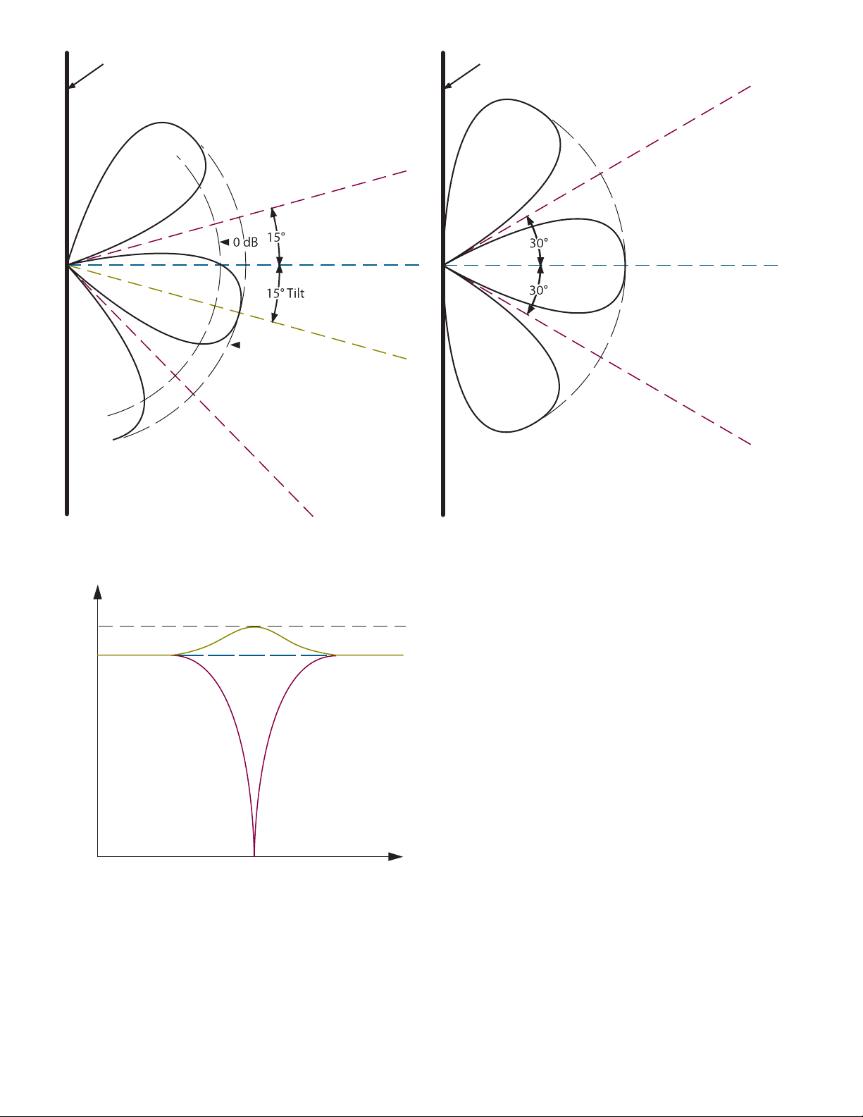
What distinguishes the Linkwitz-Riley crossover design from others is its perfect combined radiation pattern of the two drivers at the crossover point. Stanley
P. Lipshitz [3] coined the term “lobing error” to describe this crossover characteristic. It derives from the
examination of the acoustic output plots (at crossover)
of the combined radiation pattern of the two drivers
(see Figures 1 & 2). If it is not perfect the pattern forms
a lobe that exhibits an off-axis frequency dependent tilt
with amplitude peaking.
Interpretation of Figure 1 is not particularly obvious. Let’s back up a minute and add some more details.
For simplicity, only a two way system is being modeled.
e two drivers are mounted along the vertical center
of the enclosure (there is no side-to-side displacement,
i.e., one driver is mounted on top of the other.) All
front-to-back time delay between drivers is corrected.
e figure shown is a polar plot of the sideview, i.e., the
angles are vertical angles.
It is only the vertical displacement sound field that is
at issue here. All of the popular crossover types (constant voltage [4], Butterworth all-pass [5], etc.) are well
behaved along the horizontal on-axis plane. To illustrate the geometry involved here, imagine attaching
a string to the speaker at the mid-point between the
drivers. Position the speaker such that the mid-point is
exactly at ear level. Now pull the string taut and hold
it up to your nose (go on, no one’s looking). e string
should be parallel to the floor. Holding the string tight,
move to the left and right: this is the horizontal onaxis plane. Along this listening plane, all of the classic crossover designs exhibit no problems. It is when
you lower or raise your head below or above this plane
that the problems arise. is is the crux of Siegfried
Linkwitz’s contribution to crossover design. After all
these years and as hard as it is to believe, he was the
first person to publish an analysis of what happens offaxis with non-coincident drivers (not-coaxial). (Others
may have done it before, but it was never made public
record.)
Figure 1a represents a side view of the combined
acoustic radiation pattern of the two drivers emitting
the same single frequency. at is, a plot of what is
going on at the single crossover frequency all along the
vertical plane. e pattern shown is for the popular 18
dB/octave Butterworth all-pass design with a crossover
frequency of 1700 Hz and drivers mounted 7 inches
apart1.
Linkwitz-Riley-2
Page 3
1. On-Axis
3. Canc
ellation Axis
2. P
eak
ing Axis
3. Cancellation Axis
Combined Acoustic
Radiation Pattern
Time Corrected Sound
Propagation Plane
+3 dB
Peaking
3
.
C
a
n
c
e
l
l
a
t
i
o
n
A
x
i
s
2
.
P
e
a
k
i
n
g Axis
+3
0
Amplitude (dB)
1700 Hz
Frequency (Hz)
1. On-Axis
On-Axis
Cancellation Axis
Cancellation Axi
s
Combined Acoustic
Radiation Pattern
Time Corrected Sound
Propagation Plane
0 dB
No Peaking
Figure 1a.
crossover.
Figure 1b. Butterworth all-pass design radiation pattern at
Figure 2. Linkwitz-Riley radiation response at crossover.
What is seen is a series of peaking and cancellation
nodes. Back to the string: holding it taut again and
parallel to the floor puts you on-axis. Figure 1a tells us
that the magnitude of the emitted 1700 Hz tone will
be 0 dB (a nominal reference point). As you lower your
head, the tone increases in loudness until a 3 dB peak is
reached at 15 degrees below parallel. Raising your head
above the on-axis line causes a reduction in magnitude
until 15 degrees is reached where there is a complete
cancellation of the tone. ere is another cancellation
axis located 49 degrees below the on-axis. Figure 1b
depicts the frequency response of the three axes for
reference.
For a constant voltage design, the response looks
worse, having a 6 dB peaking axis located at -20 degrees and the cancellation axes at +10 and -56 degrees,
respectively. e peaking axis tilts toward the lagging
driver in both cases, due to phase shift between the
two crossover outputs.
e cancellation nodes are not due to the crossover
design, they are due to the vertically displaced drivers. (e crossover design controls where cancellation
nodes occur, not that they occur.) e fact that the
Linkwitz-Riley-3
Page 4
On Axis
Ca
ncellation Axis
Pe
ak
ing Axis
Cancellation Axis
Figure 3. Butterworth all-pass crossover stage-audience relationship.
On Axis
Ca
nc
e
llat
ion Axis
Cancellation Axis
Figure 4. Linkwitz-Riley crossover stage-audience relationship.
drivers are not coaxial means that any vertical deviation from the on-axis line results in a slight, but very
significant difference in path lengths to the listener.
is difference in distance traveled is effectively a
phase shift between the drivers. And this causes cancellation nodes — the greater the distance between
drivers, the more nodes.
In distinct contrast to these examples is Figure
2, where the combined response of a Linkwitz-Riley
crossover design is shown. ere is no tilt and no peaking — just a perfect response whose only limitation is
the dispersion characteristics of the drivers. e main
contributor to this ideal response is the in-phase relationship between the crossover outputs.
Linkwitz-Riley-4
Two of the cancellation nodes are still present, but
are well defined and always symmetrical about the
on-axis plane. eir location changes with crossover
frequency and driver mounting geometry (distance
between drivers). With the other designs, the peaking
and cancellation axes change with frequency and driver
spacing.
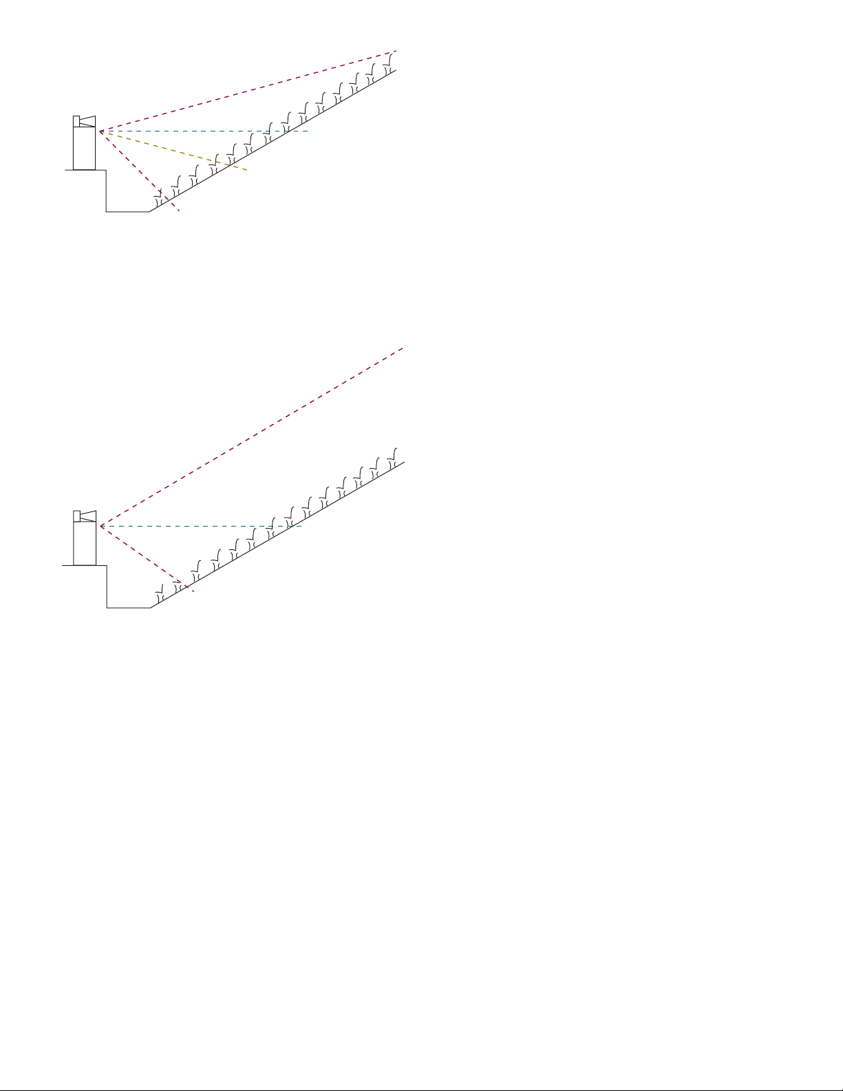
Let’s drop the string and move out into the audience
to see how these cancellation and peaking nodes affect
things. Figure 3 shows a terribly simplified, but not too
inaccurate stage-audience relationship with the characteristics of Figure 1 added.
e band is cooking and then comes to a musical
break. All eyes are on the flautist, who immediately goes
into her world-famous 1700 Hz solo. So what happens?
e people in the middle hear it sweet, while those up
front are blown out of their seats, and those in the back
are wondering what the hell all the fuss is!
Figure 4 shows the identical situation but with the
Linkwitz-Riley characteristics of Figure 2 added. Now
the people in the middle still hear everything sweet,
but those up front are not blown away, and those in the
back understand the fuss!
I think you get the point.
Now let’s get real. I mean really real. e system isn’t
two way, it is four way. ere isn’t one enclosure, there
are sixteen. No way are the drivers 7 inches apart — try
27 inches. And time corrected? Fuhgeddaboudit.
Can you even begin to imagine what the vertical
off-axis response will look like with classic crossover
designs? e further apart the drivers are, the greater
the number of peaks and cancellations, resulting in a
multi-lobe radiation pattern. Each crossover frequency
has its own set of patterns, complicated by each enclosure contributing even more patterns. And so on.
(For large driver spacing the Linkwitz-Riley design
has as many lobes as other designs, except that the
peaks are always 0 dB, and the main lobe is always
on-axis.)
Note that all this is dealing with the direct sound
field, no multiple secondary arrivals or room interference or reverberation times are being considered. Is it
any wonder that when you move your real-time analyzer microphone three feet you get a totally different
response?
Now let me state clearly that using a Linkwitz-Riley
crossover will not solve all these problems. But it will
go a long way toward that goal.
Page 5
-3
0
Amplitude (dB)
Frequency (Hz)
2
4
d
B
/
o
c
t
1
8
d
B
/
o
c
t
12 dB / oc
t
-6
-10
-20
-30
-40
f
o
2f
o
f
o
/2
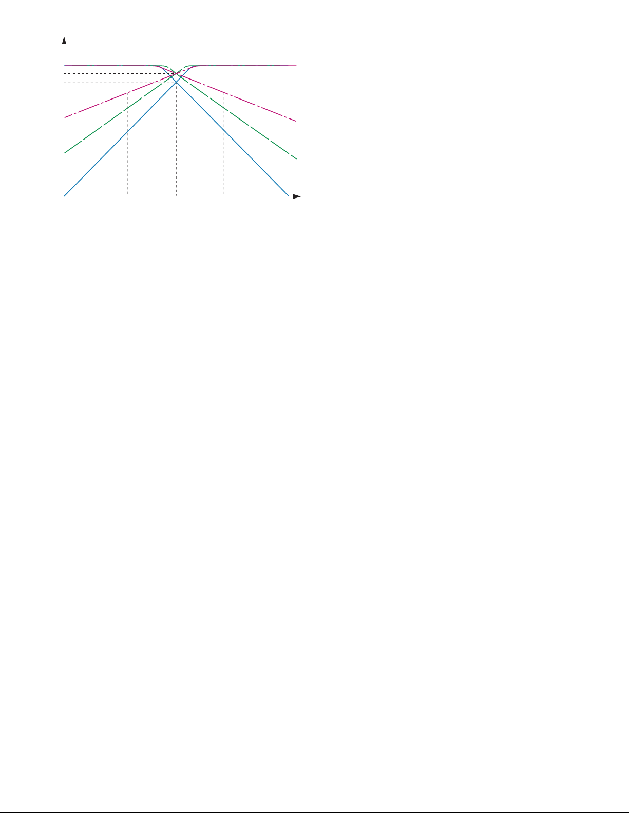
Figure 5. Frequency response of 4th-order Linkwitz-Riley crossover.
witz-Riley alignment is the rolloff rate of 24 dB/octave
(Figure 5). With such a sharp drop-off, drivers can
operate closer to their theoretical crossover points
without the induced distortion normally caused by
frequencies lying outside their capabilities. Frequencies just one octave away from the crossover point are
already attenuated by 24 dB (a factor or about 1/16).
e importance of sharp cutoff rate and in-phase frequency response of the crossover circuitry cannot be
over-stressed in contributing to smooth overall system
response.
Linkwitz-Riley crossover characteristics summary:
1. Absolutely flat amplitude response throughout the
2. e acoustic sum of the two driver responses is unity
3. Zero phase difference between drivers at crossover.
4. e low pass and high pass outputs are everywhere
5. All drivers are always wired the same (in phase).
this is, indeed, the perfect crossover. But such is not so.
e wrinkle involves what is known as “linear phase.”
e other outstanding characteristic of the Link-
passband with a steep 24 dB/octave rolloff rate after
the crossover point.
at crossover. (Amplitude response of each is -6 dB
at crossover, i.e., there is no peaking in the summed
acoustic output.)
(Lobing error equals zero, i.e., no tilt to the polar radiation pattern.) In addition, the phase difference of
zero degrees through crossover places the lobe of the
summed acoustic output on axis at all frequencies.
in phase. (is guarantees symmetry of the polar
response about the crossover point.)
A casual reading of the above list may suggest that
A Linkwitz-Riley crossover alignment is not linear
phase: meaning that the amount of phase shift is a
function of frequency. Or, put into time domain terms,
the amount of time delay through the filter is not
constant for all frequencies, which means that some
frequencies are delayed more than others. (In technical
terms, the network has a frequency-dependent group
delay, but with a gradually changing characteristic.)
Is this a problem? Specifically, is this an audible
“problem?” In a word, no.
Much research has been done on this question [69] with approximately the same conclusions: given a
slowly changing non-linear phase system, the audible
results are so minimal as to be nonexistent; especially
in the face of all of the other system nonlinearities.
And with real-world music sources (remember music?),
it is not audible at all.
State-Variable Solution
One of the many attractions of the Linkwitz-Riley design is its utter simplicity, requiring only two standard
2nd-order Butterworth filters in series. e complexities occur when adjustable crossover frequencies are
required.
After examining and rejecting all of the standard
approaches to accomplish this task, Rane developed
a 4th-order state-variable filter specifically for implementing the Linkwitz-Riley crossover. e state-variable topology was chosen over other designs for the
following reasons:
1. It provides simultaneous high-pass and low-pass out-
puts that are always at exactly the same frequency.
2. Changing frequencies can be done simultaneously
on the high-pass and low-pass outputs without any
changes in amplitude or Q (quality factor).
3. e sensitivities of the filter are very low. (Sensitivity
is a measure of the effects of non-ideal components
on an otherwise, ideal response.)
4. It offers the most cost-effective way to implement
two 4th-order responses with continuously variable
crossover frequencies.
Linkwitz-Riley-5
Page 6
R
C
R
C
INPUT
HF OUTPUT
LF OUTPUT
Figure 6. Driver Displacement
Figure 7a. Without time alignment
Time or Phase Correction
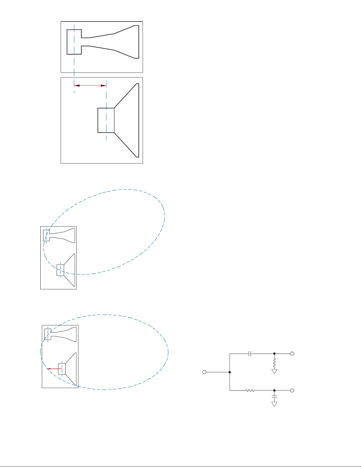
Implicit in the development of the theory of a Linkwitz-Riley crossover design is the key assumption that
the sound from each driver radiates from the some
exact vertical plane, i.e., that the drivers have no time
delay with respect to each other. e crossover then
prohibits any lobing errors as the sound advances
forward simultaneously from the two drivers. Figure
6 illustrates such a front-to-back displacement, which
causes the lobing error shown in Figure 7a.
A Linkwitz-Riley crossover applied to drivers that
are not time-corrected loses most of its magic. e
lobing error is no longer zero; it exhibits a frequency
dependent tilt with magnitude errors as shown in Figure 7a.
Crossover Primer
1st-Order Network
Analog crossovers begin with a resistor and a capacitor.
It never gets more complicated than that—just resistors
and capacitors: lots and lots of resistors and capacitors.
Resistors are the great emancipators of electronics;
they are free of frequency dependence. ey dissipate
energy without frequency prejudice. All frequencies
treated equally. Capacitors, on the other hand, selectively absorb energy; they store it, to be released at a
later time. While resistors react instantly to any voltage
changes within a circuit, capacitors take time to charge
and discharge.
Capacitors are so frequency dependent they only
pass signals with frequency associated with them. Direct-current (think of it as zero frequency) will not pass
at all, while at the other end of the spectrum very high
frequencies will not absorb. Capacitors act like a piece
of wire to high frequencies; hardly there at all.
phase of both drivers, reducing lobing error.
Linkwitz-Riley-6
Figure 7b. With time alignment
Figure 8. 1st-order crossover networkFigure 7. Adding delay to the forward driver time-aligns the
Page 7
We use these facts to create a crossover network.
Figure 8 shows such a circuit. By interchanging the positions of the resistor and capacitor, low-pass (low frequencies = LF) and high-pass (high frequencies = HF)
filters result. For the low-pass case (LF), the capacitor
ignores low frequencies and shunts all high frequencies
to ground. For the high-pass case (HF), the opposite
occurs. All low frequencies are blocked and only high
frequencies are passed.
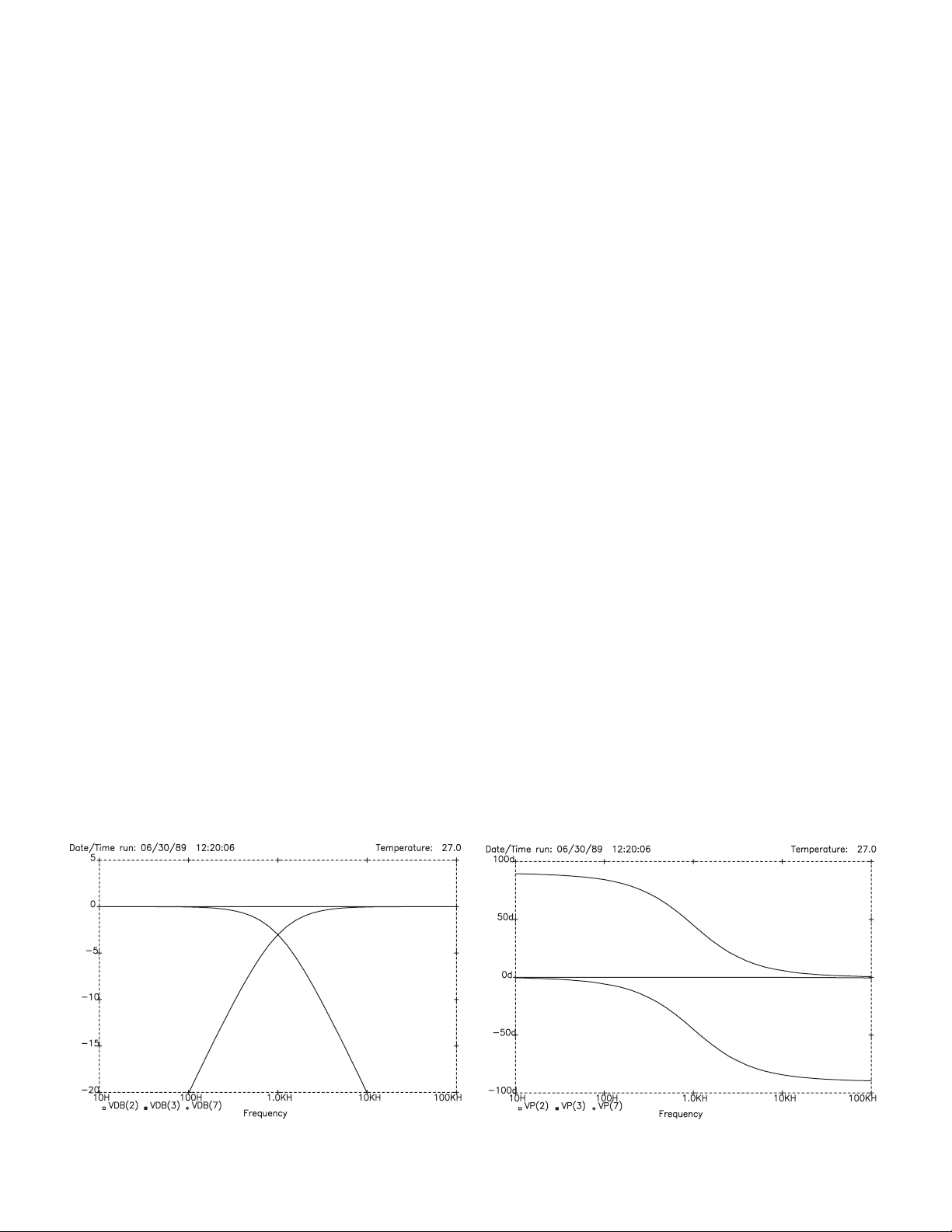
1st-Order Amplitude Response
Using 1 kHz as an example and plotting the amplitude
versus frequency response (Figure 9) reveals the expected low-pass and high-pass shapes. Figure 9 shows
that the 1st-order circuit exhibits 6 dB/octave slopes.
Also, that 6 dB/octave equals 20 dB/decade. Both
ways of expressing steepness are useful and should be
memorized. e rule is: each order, or degree, of a
filter increases the slopes by 6 dB/octave or 20 dB/
decade. So, for example, a 4th-order (or 4th-degree—
interchangeable terms) circuit has 24 dB/octave (4 x 6
dB/octave) or 80 dB/decade (4 x 20 dB/decade) slopes.
Using equal valued resistors and capacitors in each
of the circuits causes the amplitude responses to ‘cross
over’ at one particular frequency where their respective -3 dB points intersect. is point represents the
attenuation effect resulting when the impedance of the
capacitor equals the resistance of the resistor.
e equivalent multiplying factor for -3 dB is .707,
i.e., a signal attenuated by 3 dB will be .707 times the
original in level. Ohms law tells us that if the voltage is
multiplied by .707, then the current will also be multiplied by .707. Power is calculated by multiplying voltage
times current. erefore, a voltage multiplied by .707,
and a current multiplied by .707, equals 0.5 power. So
the -3 dB points represent the half-power point — a
useful reference.
Lastly, Figure 9 shows the flat amplitude response
resulting from summing the LF and HF outputs together. is is called constant voltage, since the result
of adding the two output voltages together equals
a constant. e 1st-order case is ideal in that con-
stant power also results. Constant-power refers to the
summed power response for each loudspeaker driver
operating at the crossover frequency. is, too, results
in a constant. Since each driver operates at half-power
at the crossover frequency, their sum equals one—or
unity, a constant.
1st-Order Phase Response
Much is learned by examining the phase shift behavior
(Figure 10) of the 1st-order circuit. e upper curve is
the HF output and the lower curve is the LF output.
e HF curve starts at +90° phase shift at DC, reduces
to +45° at the crossover frequency and then levels out
at 0° for high frequencies. e LF curve starts with 0o
phase shift at DC, has -45° at the crossover frequency
and levels out at -90° for high frequencies.
Because of its reactive (energy storing) nature each
capacitor in a circuit contributes 90° of phase shift,
either positive or negative depending upon its application. Since the HF section places the capacitor directly
in the signal path, this circuit starts out with +90°
phase shift. is is called phase lead. e LF section,
which starts out with 0° and eventually becomes -90° is
called phase lag.
Examination of Figure 10 allows us to formulate a
new rule: each order, or degree, of a crossover net-
work contributes ±45° of phase shift at the crossover
frequency (positive for the HF output and negative for
the LF output).
Figure 9. 1st-order amplitude response. Figure 10. 1st-order phase response.
Linkwitz-Riley-7
Page 8
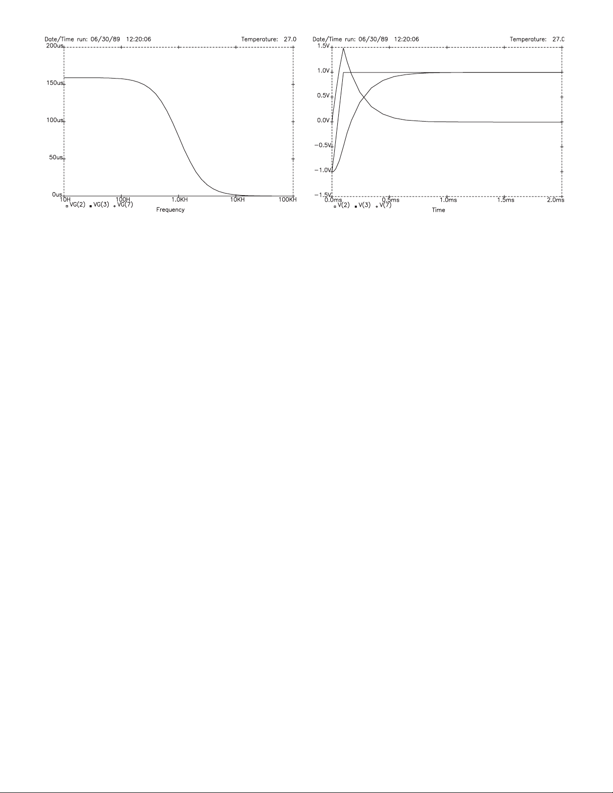
Figure 11. 1st-order group delay response.
Figure 12. 1st-order transient response.
Once again, Figure 10 shows the idealized nature
of the 1st-order case. Here the result of summing the
outputs together produces 0° phase shift, which is to
say that the summed amplitude and phase shift of a
1st-order crossover is equivalent to a piece of wire.
1st-Order Group Delay Response
We shall return to our rules shortly, but first the
concept of group delay needs to be introduced. Group
delay is the term given to the ratio of an incremental
change in phase shift divided by the associated incremental change in frequency (from calculus, this is the
first-derivative). e units for group delay are seconds.
If the phase shift is linear, i.e., a constant rate of change
per frequency step, then the incremental ratio (first-derivative) will be constant. We therefore refer to a circuit
with linear phase shift as having constant group delay.
Group delay is a useful figure of merit for identifying
linear phase circuits. Figure 11 shows the group delay
response for the Figure 8 1st-order crossover circuit.
Constant group delay extends out to the crossover
region where it gradually rolls off (both outputs are
identical). e summed response is, again, that of a
piece of wire.
e importance of constant group delay is the ability
to predict the behavior of the LF output step response.
A circuit with constant group delay (linear phase shift)
shows no overshoot or associated damping time to a
sudden change (step) in input level (Figure 12). e
circuit reacts smoothly to the sudden change by rising
steadily to meet the new level. It does not go beyond
the new level and require time to settle back. We also
refer to the step response as the transient response of
the circuit. e transient response of the summed outputs is perfect since their sum is perfectly equal to one.
For clarity purposes normally only the step response
of the LF network is shown. Nothing is learned by
examining the step response of the HF network. A step
response represents a transition from one DC level to
another DC level, in this case, from -1 volt to +1 volt.
A HF network, by definition, does not pass DC (neither
does a loudspeaker), so nothing particularly relevant
is learned by examining its step response. To illustrate
this, Figure 12 shows the HF step response. It begins
and ends with zero output since it cannot pass DC. e
sharp edge of the input step, however, contains much
high frequency material, which the HF network passes.
So, it begins at zero, passes the high frequencies as a
pulse, and returns to zero.
e HF and LF outputs are the exact complement of
each other. eir sum equals the input step exactly as
seen in Figure 12. Still, we learn everything we need to
know by examining only the LF step response; looking
for overshoot and ringing. From now on, just the LF
output is shown.
Linkwitz-Riley-8
Page 9
a) 1st-order
(6 dB/oct)
b) 2nd-order
(12 dB/oct)
c) 3rd-order
(18 dB/oct)
d) 4th-order
(24 dB/oct)
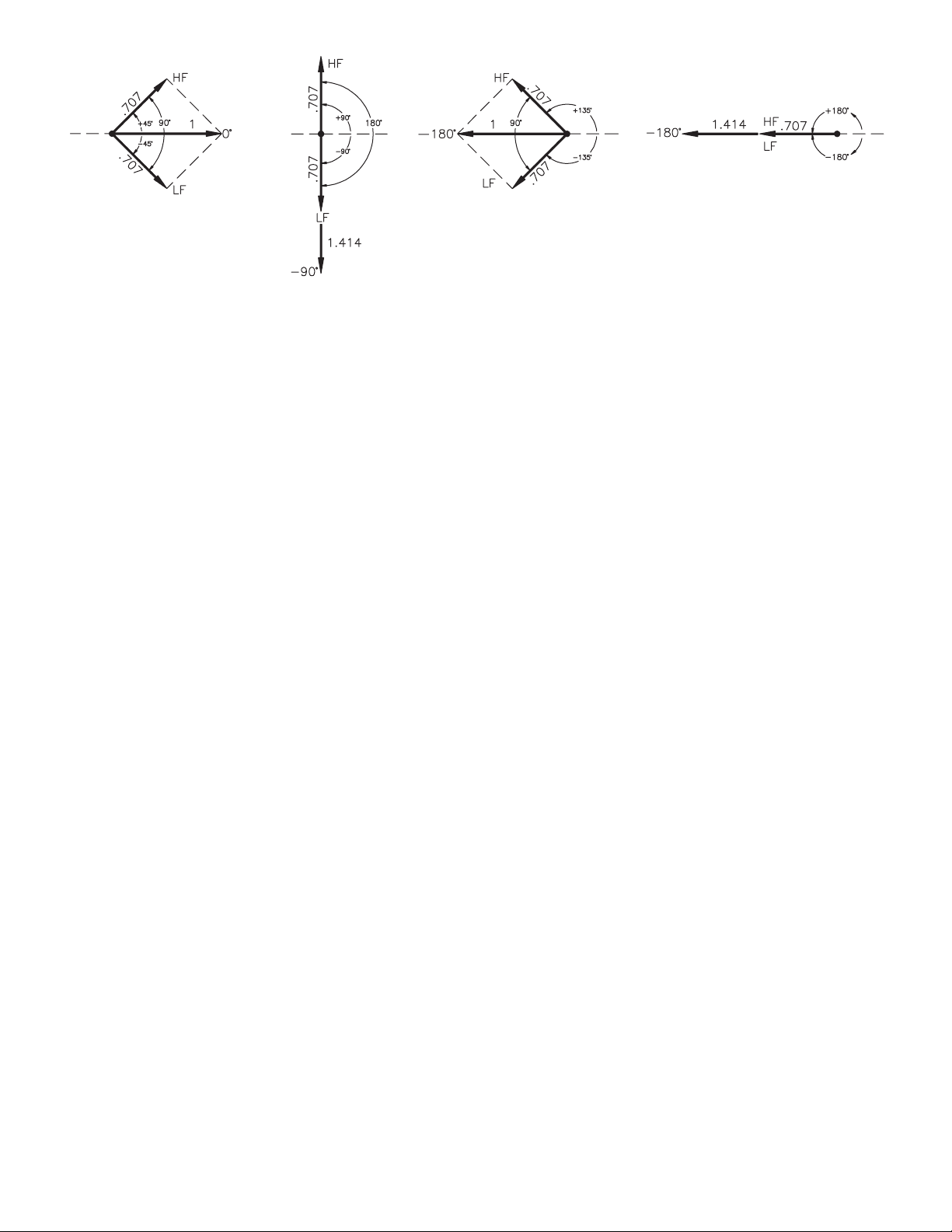
Figure 13. 1st-order vector and 2nd-, 3rd- and 4th-order Butterworth vector diagrams.
Vector Diagrams
A vector is a graphical thing (now we’re getting technical) with magnitude and direction. We can use vectors
to produce diagrams representing the instantaneous
phase shift and amplitude behavior of electrical circuits. In essence, we freeze the circuit for a moment of
time to examine complex relationships.
We shall now apply our two rules to produce a
vector diagram showing the relative phase shift and
amplitude performance for the 1st-order crossover
network at the single crossover frequency (Figure 13a).
By convention, 0° points right, +90° points up, -90°
points down, and ±180° points left. From Figures 9 &
10 we know the HF output amplitude is -3 dB with +45°
of phase shift at 1 kHz, and the LF output is -3 dB with
-45° phase shift. Figure 13a represents the vectors as
being .707 long (relative to a normalized unity vector)
and rotated up and down 45°. is shows us the relative
phase difference between the two outputs equals 90°.
Next we do vector addition to show the summed
results. Vector addition involves nothing more complex than mentally moving one of the vectors to the
end of the other and connecting the center to this new
end point (constructing a parallelogram). Doing this,
results in a new vector with a length equal to 1 and an
angle of 0°. is tells us the recombined outputs of the
HF and LF networks produce constant voltage (i.e., a
vector equal to 1), and is in phase with the original input of the circuit (i.e., a vector with 0° phase rotation).
e 1st-order case is ideal when summed. It yields a
piece of wire. Since the responses are the exact mirror images of each other, they cancel when summed,
thus behaving as if neither was there in the first place.
Unfortunately, all optimized higher order versions yield
flat voltage/power response, group delay or phase shift,
but not all at once. Hence, the existence of different
alignments and resultant compromises.
Comparing Butterworth &
Linkwitz-Riley Alignments
Butterworth Alignment
ere are many types of crossover alignments or filters
(most named after mathematicians). Each displays a
unique amplitude characteristic throughout the passband. Of these, only Butterworth filters have an absolutely flat amplitude response. For this reason, Butterworth filters are popular for crossover use. Butterworth
filters obey our two rules, so we can diagram them for
the 2nd, 3rd and 4th-order cases (Figures 13b-13d).
e 2nd-order case has ±90° phase shift as shown. is
results in the outputs being 180° out of phase. Vector
addition for this case produces a zero length vector, or
complete cancellation. e popular way around this is
to reverse the wiring on one of the drivers (or, if available, electronically inverting the phase at the crossover). is produces a resultant vector 90° out of phase
with the input and 3 dB (1.414 equals +3 dB) longer.
is means there will be a 3 dB amplitude bump at the
crossover region for the combined signals.
e 3rd-order Butterworth case (Figure 13c) mimics the 1st-order case at the crossover frequency, except
rotated 180°. Hence, we see the HF vector rotated up
135° (3 x 45°) and the LF vector rotated down the same
amount. e phase shift between outputs is still 90°.
e resultant is constant voltage (unity) but 180° outof-phase with the input.
e 4th-order Butterworth diagram (Figure 13d)
shows the HF vector rotated up 180° and the LF vector
rotated down the same amount. e phase difference
between outputs is now zero, but the resultant is +3 dB
and 180° out-of-phase with the input. So, the 4th-order
and the inverted phase 2nd-order produce 3 dB bumps
at the crossover frequency.
Linkwitz-Riley-9
Page 10
a) 2nd-order LR-2
(12 dB/oct)
b) 4th-order LR-4
(24 dB/oct)
c) 8th-order LR-8
(48 dB/oct)
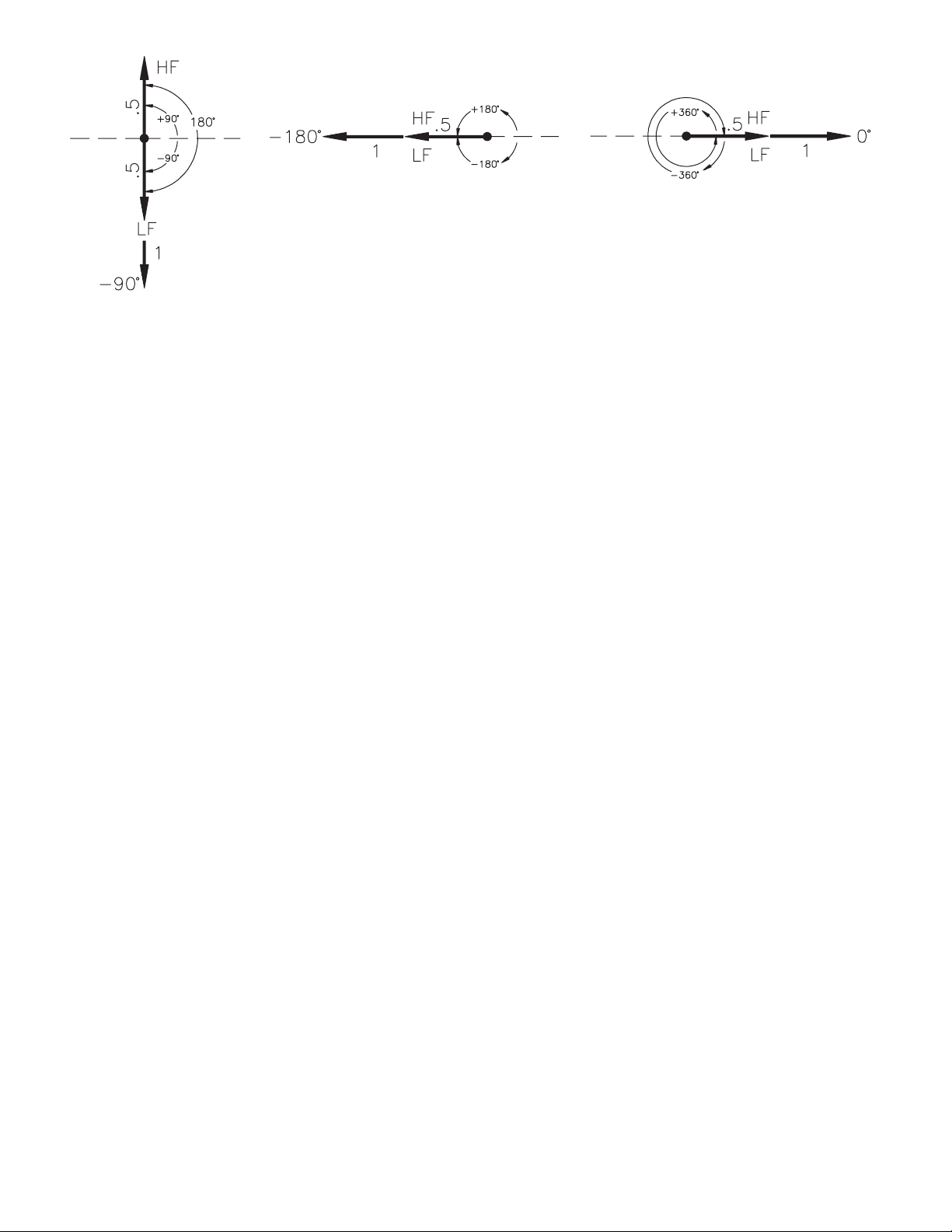
Figure 14. Linkwitz-Riley vector diagrams for 2nd- to 8th-order cases.
Linkwitz-Riley Alignment
Two things characterize a Linkwitz-Riley alignment:
1. In-phase outputs (0° between outputs) at all frequencies (not just at the crossover frequency as popularly
believed by some).
2. Constant voltage (the outputs sum to unity at all
frequencies).
As discussed earlier Linkwitz-Riley in-phase outputs
solve one troublesome aspect of crossover design. e
acoustic lobe resulting from both loudspeakers reproducing the same frequency (the crossover frequency)
is always on-axis (not tilted up or down) and has no
peaking. is is called zero lobing error. In order for
this to be true, however, both drivers must be in correct time alignment, i.e., their acoustic centers must lie
in the same plane (or electrically put into equivalent
alignment by adding time delay to one loudspeaker).
Failure to time align the loudspeakers defeats this zero
lobing error aspect. (e lobe tilts toward the lagging
loudspeaker.)
Examination of Figure 13 shows that the 2nd-order
(inverted) and 4th-order Butterworth examples satisfy
condition 1, but fail condition 2 since they exhibit a 3
dB peak. So, if a way can be found to make the amplitudes at the crossover point -6 dB instead of -3 dB,
then the vector lengths would equal 0.5 (-6 dB) instead
of .707 (-3 dB) and sum to unity — and we would have a
Linkwitz-Riley crossover.
Russ Riley suggested cascading (putting in series)
two Butterworth filters to create the desired -6 dB
crossover points (since each contributes -3 dB). Voila!
Linkwitz-Riley alignments were born.
Taken to its most general extremes, cascading any
order Butterworth filter produces 2x that order Linkwitz-Riley. Hence, cascading two 1st-order circuits produces a 2nd-order Linkwitz-Riley (LR-2); cascading two
2nd-order Butterworth filters creates a LR-4 design;
cascading two 3rd-order Butterworth filters gives a LR6, and so on. (Starting with LR-2, every other solution
requires inverting one output. at is, LR-2 and LR-6
need inverting, while LR-4 and LR-8 do not.)
LR-2, Transient Perfect 2nd-Order Crossover
As an example of this process, let’s examine a LR-2 design. Referring to Figure 8 all that is required is to add
a buffer amplifier (to avoid interaction between cascaded filter components) to each of these two outputs and
then add another resistor/capacitor network identical
to the first. We now have a 2nd-order Linkwitz-Riley
crossover.
e new vector diagram looks like Figure 14a. Each
vector is .5 long (from the fact that each 1st-order
reduces by 0.707, and .707 x .707 = .5) with phase angles
of ±90°. Since the phase difference equals 180°, we invert one before adding and wind up with a unity vector
90° out of phase with the original.
Figure 15 shows the amplitude response. e crossover point is located at -6 dB and the slopes are 12 dB/
octave (40 dB/decade). e summed response is perfectly flat. Figure 16 shows the phase response. At the
crossover frequency we see the HF output (upper trace)
has +90° phase shift, while the LF output (lower trace)
has -90° phase shift, for a total phase difference of 180°.
Invert one before summing and the result is identical
to the LF output.
ese results differ from the 1st-order case in that
the summed results do not yield unity (a piece of wire),
but instead create an all-pass network. (An all-pass
network is characterized by having a flat amplitude
response combined with a smoothly changing phase
response.) is illustrates Garde’s [10] famous work.
Linkwitz-Riley-10
Page 11
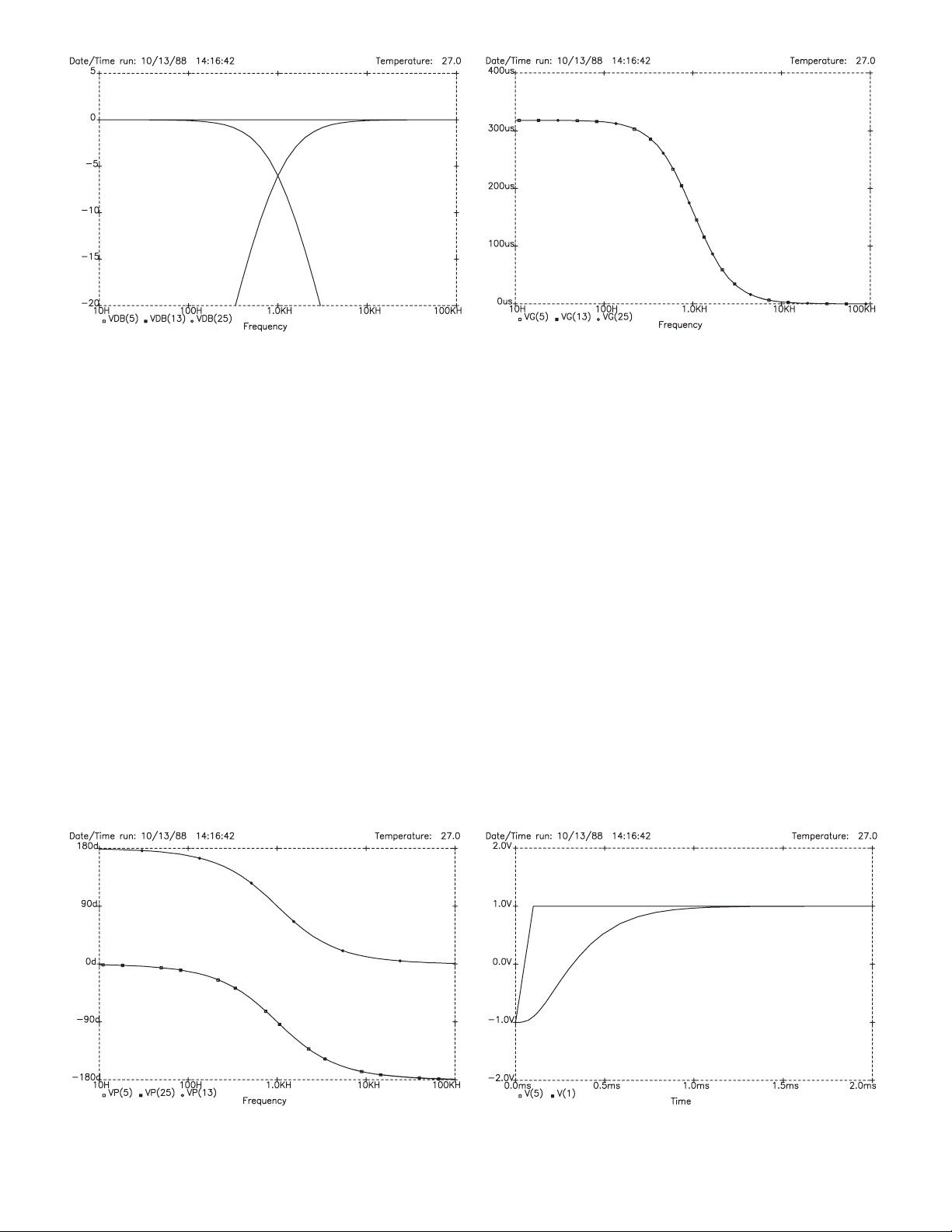
Figure 15. LR-2 amplitude response
Figure 17. LR-2 group delay
Cascading two linear phase circuits results in linear
phase, as shown by the constant group delay plots (all
three identical) of Figure 17. And constant group delay
gives the transient perfect LF step response shown in
Figure 18.
LR-4 and LR-8 Alignments
Looking back to Figure 14b. we see the vector diagrams
for 4th and 8th-order Linkwitz-Riley designs. e LR-4
design shows the resultant vector is unity but 180° out
of phase with the input at the crossover frequency.
Cascading two 4th-order Butterworth filters results
in an 8th-order Linkwitz-Riley design. Figure 14c.
shows the vector diagram for the LR-8 case. Here, we
see the phase shift for each output undergoes 360° rota-
tion returning to where it began. e resultant vector
is back in phase with the original input signal. So, not
only are the outputs in phase with each other (for all
frequencies), they are also in phase with the input (at
the crossover frequency).
8th-Order Comparison
A LR-8 design exhibits slopes of 48 dB/octave, or 160
dB/decade. Figure 19 shows this performance characteristic compared with the LR-4, 4th-order case for
reference. As expected, the LR-4 is 80 dB down one
decade away from the corner frequency, while the LR-8
is twice that, or 160 dB down. Of interest here, are the
potential benefits of narrowing the crossover region by
using a LR-8 alignment.
Figure 16. LR-2 phase response
Figure 18. LR-2 transient response
Linkwitz-Riley-11
Page 12
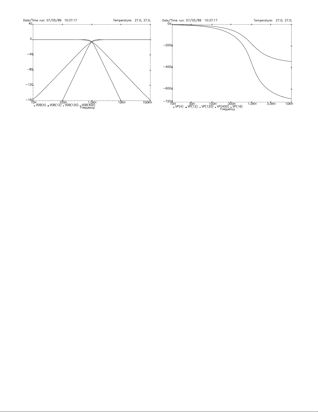
Figure 19. LR-4 and LR-8 slopes
Figure 20. LR-4 and LR-8 phase response
Figure 21 magnifies the responses shown in Figure
19 to reveal a clearer picture of the narrower crossover
region, as well as showing the flat summed responses.
(e slight difference in summed amplitudes at the
crossover frequency is due to a slight gain difference
between the two circuits.) e critical crossover region
for the LR-8 case is one-half of what it is for the LR-4
case. e exact definition of where the crossover region
begins and ends is ambiguous, but, by whatever definition, the region has been halved.
As an example of this, a very conservative definition might be where the responses are 1 dB down from
their respective passbands. We would then refer to the
crossover region as extending from the -1 dB point on
the low-pass response to the -1 dB point on the highpass response. For LR-8, these points are 769 Hz and
1301 Hz respectively, yielding a crossover region only
¾-octave wide. As a comparative reference, the LR-4
case yields -1 dB points at 591 Hz and 1691 Hz, for a
1.5-octave wide region.
For the LR-8 case, it is interesting to note that the
-1 dB point on the low-pass curve corresponds almost
exactly to the -20 dB point on the high-pass curve
(the exact points occur at 760 Hz and 1316 Hz). So if
you want to define the region as where the response is
down 20 dB, you get the same answer. e entire region for the LR-8 case is ¾-octave wide, or it is one-half
this number for each driver. at is, the loudspeaker
driver (referred to as ‘driver’ from now on) has to be
well behaved for only about 0.4-octave beyond the
crossover point. is compares with the 4th-order case
where the same driver must behave for 0.8-octave.
e above is quite conservative. If other reference
points are used, say, the -3 dB points (895 Hz & 1117
Hz), then the LR-8 crossover region is just ⅓-octave
wide, and drivers only have to stay linear for 1/6-octave. (1/6-octave away from the crossover frequency the
drive signal is attenuated by 12 dB, so the output driver
is operating at about 1/16 power.)
e extremely steep slopes offer greater driver protection and linear operation. Beyond the driver’s linear
limits all frequencies attenuate so quickly that most
nonlinearities and interaction ceases being significant.
Because of this, the driver need not be as well behaved
outside the crossover frequency. It is not required to reproduce frequencies it was not designed for. For similar
reasons, power handling capability can be improved for
HF drivers as well. And this narrower crossover region
lessens the need for precise driver time alignment since
the affected spectrum is so small.
e caveat, though, is an increased difficulty in
designing good systems with sharp slopes. e loudspeakers involved have differing transient responses,
polar patterns and power responses. is means the
system designer must know the driver characteristics
thoroughly. Ironically, sometimes loudspeaker overlap
helps the system blend better even when on-axis amplitude response is flat.
LR-8 Phase Response
Figure 20 shows the respective phase response for LR-4
(upper trace) and LR-8 (lower trace) designs. As predicted by the vector diagram in Figure 14b, the LR-4
case has 180° (4 x 45°) of phase shift at the crossover
Linkwitz-Riley-12
Page 13
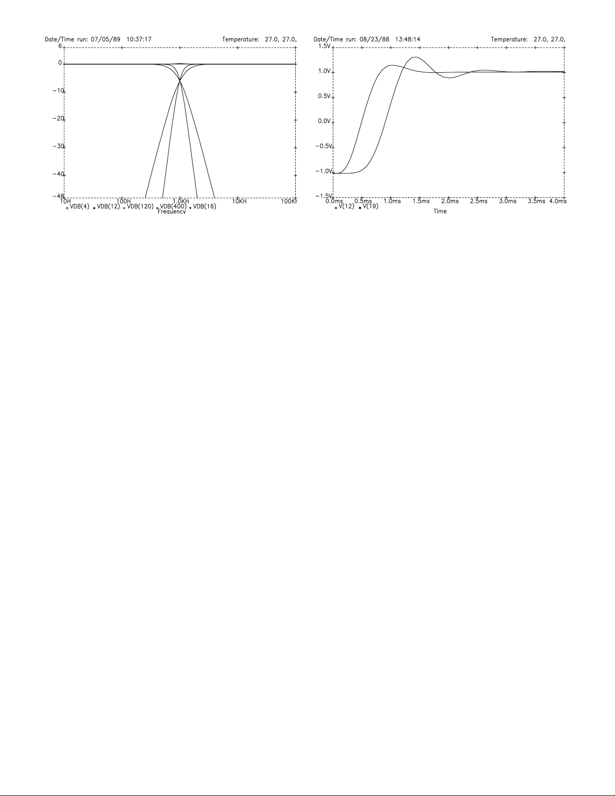
Figure 21. LR-4 and LR-8 slopes magnied
Figure 22. LR-4 and LR-8 transient response
frequency. us, the output signal is out-of-phase with
the input signal at the crossover frequency for the LR-4
case. Both outputs are in-phase with each other, but
out-of-phase with the input.
e LR-8 design eliminates this out-of-phase condition by bringing the outputs back in sync with the
input signal at the crossover frequency. e lower trace
shows the 360° phase shift for the LR-8 alignment.
LR-8 Transient Response
Butterworth functions do not have linear phase shift
and consequently do not exhibit constant group delay.
(First-order networks are not classified as Butterworth.)
Since Linkwitz-Riley designs (higher than LR-2) are
cascaded Butterworth, they also do not have constant
group delay.
Group delay is just a measure of the non-linearity
of phase shift. A direct function of non-linear phase
behavior is overshoot and damping time for a step
response. e transient behavior of all Linkwitz-Riley
designs (greater than 2nd-order) is classic Butterworth
in nature. at is, the filters exhibit slight overshoot
when responding to a step response, and take time to
damp down.
Figure 22 compares LR-8 and LR-4 designs and
shows the greater overshoot and damping time for the
8th-order case. e overshoot is 15% for the LR-4 case
and twice that, or about 30%, for the LR-8 case. As
expected, the LR-8 design takes about twice as long to
damp down. e initial rise-time differences are due to
the group delay value differences.
Is It Audible?
e conservative answer says it is not audible to the
overwhelming majority of audio professionals. Under
laboratory conditions, some people hear a difference on
non-musical tones (clicks and square waves).
e practical answer says it is not audible to anyone
for real sound systems reproducing real audio signals.
Linkwitz-Riley Power Response
Linkwitz-Riley alignments produce constant voltage
response (voltage vectors sum to unity) at the crossover
frequency, but they may produce constant power. At
the crossover frequency, each voltage output is half of
normal. is produces half the normal current into
the loudspeakers. Since power is the product of voltage times current, the power is one-quarter of normal.
Considering a simple two-way system, the combined
total power at the crossover frequency will be half of
normal (one-quarter from each driver), producing a dip
of 3 dB at the crossover frequency in the overall power
response, provided there is no additional phase shift
contributed by the drivers themselves — such is never
the case.
e power response of loudspeakers with noncoincident drivers is a complex problem. See the Vanderkooy
and Lipshitz [11] study for complete details.
Linkwitz-Riley-13
Page 14

References
1. S. H. Linkwitz “Active Crossover Networks for Non-coincident Drivers,” J. Audio Eng. Soc., vol. 24, pp. 2-8 (Jan/
Feb 1976).
2. D. Bohn. “A Fourth Order State Variable Filter for Linkwitz-Riley Active Crossover Designs,” presented at the
74th Convention of the Audio Engineering Society, New York, Oct. 9-12, 1983, preprint no. 2011.
3. S. P. Lipshitz and J. Vanderkooy, “A Family of Linear-Phase Crossover Networks of High Slope Derived by Time
Delay,” J. Audio Eng. Soc., vol. 31, pp. 2-20 (Jan/Feb 1983).
4. R. H. Small, “Constant-Voltage Crossover Network Design,” J. Audio Eng. Soc., vol. 19, pp. 12-19 (Jan 1971).
5. J.R. Ashley and A. L. Kaminsky. “Active and Passive Filters as Loudspeaker Crossover Networks,” J. Audio Eng.
Soc., vol. 19. pp. 494-502 (June 1971).
6. B. B. Bauer, “Audibility of Phase Shift,” Wireless World, (Apr. 1974).
7. S. P. Lipshitz, M. Pocock, and J. Vanderkooy. “On the Audibility of Midrange Phase Distortion in Audio Systems,” J. Audio Eng. Soc., vol. 30, pp. 580-595 (Sep 1982).
8. R. Lee. “Is Linear Phase Worthwhile,” presented at the 68th Convention of the Audio Engineering Society,
Hamburg, Mar 17-20, 1981, preprint no. 1732.
9. H. Suzuke, S. Morita and T. Shindo, “On the Perception of Phase Distortion,” J. Audio Eng. Soc., vol. 28, no. 9,
pp. 570-574 (Sep 1980).
10. P. Garde, ‘All-Pass Crossover Systems,’ J. Audio Eng. Soc., vol. 28, pp. 575-584 (Sep. 1980).
11. J. Vanderkooy & S.P. Lipshitz, “Power Response of Loudspeakers with Noncoincident Drivers — e Influence
of Crossover Design,” J. Audio Eng. Soc., Vol. 34, No. 4, pp. 236-244 (Apr. 1986).
©Rane Corporation 10802 47th Ave. W., Mukilteo WA 98275-5098 USA TEL 425-355-6000 FAX 425-347-7757 WEB w ww.rane.com
Linkwitz-Riley-14
 Loading...