

Page 1
160 dB Range (100 pA –10 mA)
a
FEATURES
Optimized for Fiber Optic Photodiode Interfacing
Eight Full Decades of Range
Law Conformance 0.1 dB from 1 nA to 1 mA
Single-Supply Operation (3.0 V– 5.5 V)
Complete and Temperature Stable
Accurate Laser-Trimmed Scaling:
Logarithmic Slope of 10 mV/dB (at VLOG Pin)
Basic Logarithmic Intercept at 100 pA
Easy Adjustment of Slope and Intercept
Output Bandwidth of 10 MHz, 15 V/s Slew Rate
1-, 2-, or 3-Pole Low-Pass Filtering at Output
Miniature 14-Lead Package (TSSOP)
Low Power: ~4.5 mA Quiescent Current (Enabled)
APPLICATIONS
High Accuracy Optical Power Measurement
Wide Range Baseband Log Compression
Versatile Detector for APC Loops
VSUM
Logarithmic Converter
AD8304
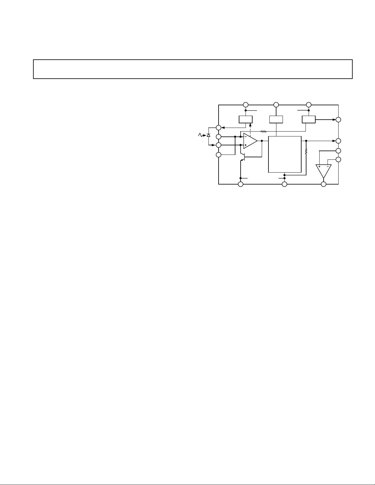
FUNCTIONAL BLOCK DIAGRAM
VPS2 PWDN VPS1
10
VPDB
6
VSUM
3
I
PD
INPT
4
5
PDB BIAS VREF
1
VNEG
~10k
2 12
TEMPERATURE
COMPENSATION
14
ACOM
0.5V
5k
AD8304
11
VOUT
13
7
8
9
VREF
VLOG
BFIN
BFNG
PRODUCT DESCRIPTION
The AD8304 is a monolithic logarithmic detector optimized for
the measurement of low frequency signal power in fiber optic
systems. It uses an advanced translinear technique to provide an
exceptionally large dynamic range in a versatile and easily used
form. Its wide measurement range and accuracy are achieved
using proprietary design techniques and precise laser trimming.
In most applications only a single positive supply, V
, of 5 V
P
will be required, but 3.0 V to 5.5 V can be used, and certain
applications benefit from the added use of a negative supply,
. When using low supply voltages, the log slope is readily
V
N
altered to fit the available span. The low quiescent current and
chip disable features facilitate use in battery-operated applications.
The input current, I
, flows in the collector of an optimally
PD
scaled NPN transistor, connected in a feedback path around a
low offset JFET amplifier. The current-summing input node
operates at a constant voltage, independent of current, with a
default value of 0.5 V; this may be adjusted over a wide range,
including ground or below, using an optional negative supply.
An adaptive biasing scheme is provided for reducing the dark
current at very low light input levels. The voltage at Pin VPDB
applies approximately 0.1 V across the diode for I
rising linearly with current to 2.0 V of net bias at I
= 100 pA,
PD
= 10 mA.
PD
The input pin INPT is flanked by the guard pins VSUM that
track the voltage at the summing node to minimize leakage.
The default value of the logarithmic slope at the output VLOG is
accurately scaled to 10 mV/dB (200 mV/decade). The resistance
at this output is laser-trimmed to 5 kΩ, allowing the slope to be
lowered by shunting it with an external resistance; the addition
of a capacitor at this pin provides a simple low-pass filter. The
intermediate voltage VLOG is buffered in an output stage that can
swing to within about 100 mV of ground (or V
tive supply, V
, and provides a peak current drive capacity of
P
) and the posi-
N
±20 mA. The slope can be increased using the buffer and a pair
of external feedback resistors. An accurate voltage reference of
2V is also provided to facilitate the repositioning of the intercept.
Many operational modes are possible. For example, low-pass filters
of up to three poles may be implemented, to reduce the output
noise at low input currents. The buffer may also serve as a comparator, with or without hysteresis, using the 2 V reference, for
example, in alarm applications. The incremental bandwidth of
a translinear logarithmic amplifier inherently diminishes for small
input currents. At the 1 nA level, the AD8304’s bandwidth is
about 2 kHz, but this increases in proportion to I
up to a
PD
maximum value of 10 MHz.
The AD8304 is available in a 14-lead TSSOP package and specified
for operation from –40°C to +85°C.
REV. A
Information furnished by Analog Devices is believed to be accurate and
reliable. However, no responsibility is assumed by Analog Devices for its
use, nor for any infringements of patents or other rights of third parties that
may result from its use. No license is granted by implication or otherwise
under any patent or patent rights of Analog Devices.
One Technology Way, P.O. Box 9106, Norwood, MA 02062-9106, U.S.A.
Tel: 781/329-4700 www.analog.com
Fax: 781/326-8703 © Analog Devices, Inc., 2002
Page 2

AD8304–SPECIFICATIONS
(VP = 5 V, VN = 0 V, TA = 25C, unless otherwise noted.)
Parameter Conditions Min1Typ Max1Unit
INPUT INTERFACE Pin 4, INPT; Pin 3 and Pin 5, VSUM
Specified Current Range Flows toward INPT Pin 100 pA
10 mA
Input Node Voltage Internally preset; may be altered 0.46 0.5 0.54 V
Temperature Drift –40°C < T
Input Guard Offset Voltage V
PHOTODIODE BIAS
2
Minimum Value I
– V
IN
Established between Pin 6, V
= 100 pA 70 100 mV
PD
< +85°C 0.02 mV/°C
SUM
A
, and Pin 4
PDB
–20 +20 mV
Transresistance 200 mV/mA
LOGARITHMIC OUTPUT Pin 8, VLOG
Slope Laser-trimmed at 25°C 196 200 204 mV/dec
0°C < T
< 70°C 194 207 mV/dec
A
Intercept Laser-trimmed at 25°C60100 140 pA
0°C < T
Law Conformance Error 10 nA < I
1 nA < I
< 70°C35175 pA
A
< 1 mA, Peak Error 0.05 0.25 dB
PD
< 1 mA, Peak Error 0.1 0.7 dB
PD
Maximum Output Voltage 1.6 V
Minimum Output Voltage Limited by V
= 0 V 0.1 V
N
Output Resistance Laser-trimmed at 25°C 4.95 5 5.05 kΩ
REFERENCE OUTPUT Pin 7, VREF
Voltage WRT Ground Laser-trimmed at 25°C 1.98 2 2.02 V
–40°C < T
< +85°C 1.92 2.08 V
A
Output Resistance 2 Ω
OUTPUT BUFFER Pin 9, BFIN; Pin 13, BFNG; Pin 11, VOUT
Input Offset Voltage –20 +20 mV
Input Bias Current Flowing out of Pin 9 or Pin 13 0.4 µA
Incremental Input Resistance 35 MΩ
Output Range R
Output Resistance 0.5 Ω
Wide-Band Noise
Small Signal Bandwidth
3
3
= 1 kΩ to ground VP – 0.1 V
L
IPD > 1 µA (see Typical Performance Characteristics) 1 µV/√Hz
IPD > 1 µA (see Typical Performance Characteristics) 10 MHz
Slew Rate 0.2 V to 4.8 V output swing 15 V/µs
POWER-DOWN INPUT Pin 2, PWDN
Logic Level, HI State –40°C < TA < +85°C, 2.7 V < VP < 5.5 V 2 V
Logic Level, LO State –40°C < TA < +85°C, 2.7 V < VP < 5.5 V 1 V
POWER SUPPLY Pin 10 and Pin 12, VPS1 and VPS2; Pin 1, VNEG
Positive Supply Voltage 3.0 5 5.5 V
Quiescent Current 4.5 5.3 mA
In Disabled State 60 µA
Negative Supply Voltage
NOTES
1
Minimum and maximum specified limits on parameters that are guaranteed but not tested are six sigma values.
2
This bias is internally arranged to track the input voltage at INPT; it is not specified relative to ground.
3
Output Noise and Incremental Bandwidth are functions of Input Current; see Typical Performance Characteristics.
4
Optional
Specifications subject to change without notice.
4
|1VP–VN| < 8V 0 –5.5 V
REV. A–2–
Page 3
AD8304
WARNING!
ESD SENSITIVE DEVICE
ABSOLUTE MAXIMUM RATINGS*
Supply Voltage VP – VN . . . . . . . . . . . . . . . . . . . . . . . . . . . 8 V
Input Current . . . . . . . . . . . . . . . . . . . . . . . . . . . . . . . 20 mA
Internal Power Dissipation . . . . . . . . . . . . . . . . . . . . 270 mW
. . . . . . . . . . . . . . . . . . . . . . . . . . . . . . . . . . . . . . 150°C/W
JA
Maximum Junction Temperature . . . . . . . . . . . . . . . . 125°C
Operating Temperature Range . . . . . . . . . . . –40°C to +85°C
Storage Temperature Range . . . . . . . . . . . . –65°C to +150°C
Lead Temperature Range (Soldering 60 sec) . . . . . . . . 300°C
*Stresses above those listed under Absolute Maximum Ratings may cause perma-
nent damage to the device. This is a stress rating only; functional operation of the
device at these or any other conditions above those indicated in the operational
section of this specification is not implied. Exposure to absolute maximum rating
conditions for extended periods may affect device reliability.
PIN CONFIGURATION
ACOM
VNEG
PWDN
VSUM
INPT
VSUM
VPDB
VREF
1
2
3
AD8304
TOP VIEW
4
(Not to Scale)
5
6
7
14
13
12
11
10
9
8
BFNG
VPS1
VOUT
VPS2
BFIN
VLOG
PIN FUNCTION DESCRIPTIONS
Pin No. Mnemonic Function
1 VNEG Optional Negative Supply, V
. This
N
pin is usually grounded; for details of
usage, see Applications section.
2PWDN Power-Down Control Input. Device is
active when PWDN is taken LOW.
3, 5 VSUM Guard Pins. Used to shield the INPT
current line.
4INPT Photodiode Current Input. Usually
connected to photodiode anode (the
photo current flows toward INPT).
6 VPDB Photodiode Biaser Output. May be
connected to photodiode cathode to
provide adaptive bias control.
7 VREF Voltage Reference Output of 2 V
8 VLOG Output of the Logarithmic Front-End
Processor; R
= 5 kΩ to ground.
OUT
9 BFIN Buffer Amplifier Noninverting Input
(High Impedance)
10 VPS2 Positive Supply, V
(3.0 V to 5.5 V)
P
11 VOUT Buffer Output; Low Impedance
12 VPS1 Positive Supply, V
(3.0 V to 5.5 V)
P
13 BFNG Buffer Amplifier Inverting Input
14 ACOM Analog Ground
ORDERING GUIDE
Model Temperature Range Package Description Package Option
AD8304ARU –40°C to +85°CTube, 14-Lead TSSOP RU-14
AD8304ARU-REEL 13" Tape and Reel
AD8304ARU-REEL7 7" Tape and Reel
AD8304-EVAL Evaluation Board
CAUTION
ESD (electrostatic discharge) sensitive device. Electrostatic charges as high as 4000 V readily
accumulate on the human body and test equipment and can discharge without detection. Although the
AD8304 features proprietary ESD protection circuitry, permanent damage may occur on devices
subjected to high energy electrostatic discharges. Therefore, proper ESD precautions are recommended
to avoid performance degradation or loss of functionality.
REV. A
–3–
Page 4
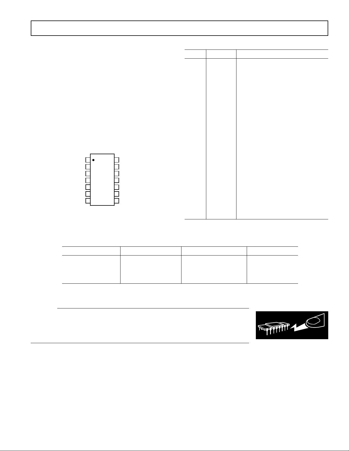
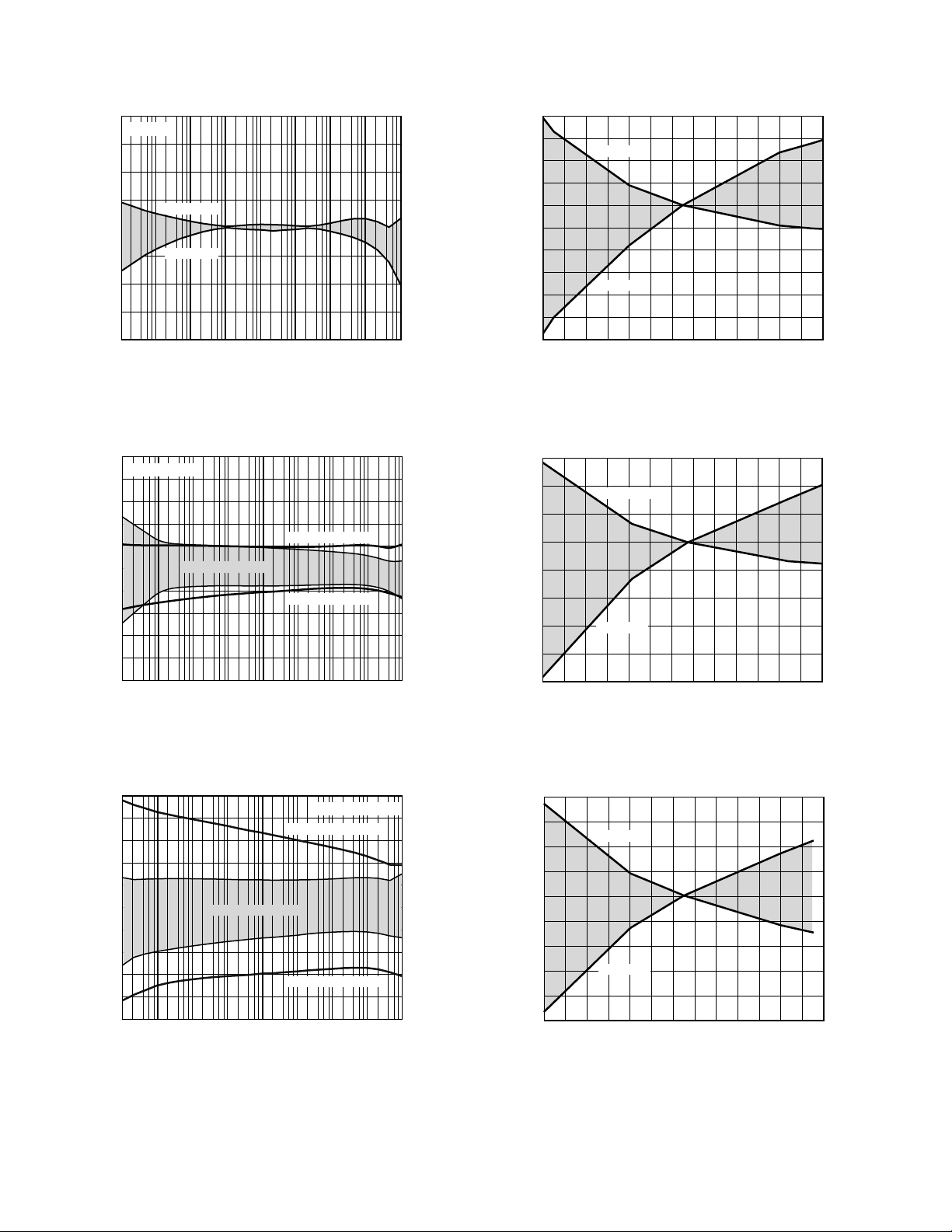
AD8304–Typical Performance Characteristics
INPUT – A
2.4
0.6
100p 10m1n
V
OUT
– V
10n 100n 1 10 100 1m
2.2
1.6
1.4
1.2
1.0
2.0
1.8
+85C
+25C
–40C
0.8
1.25
–1.00
ERROR – dB (10mV/dB)
1.00
0.25
0
–0.25
–0.50
0.75
0.50
–0.75
TA = –40C, +25C, +85C
V
P
= 3.0V
(VP = 5 V, VN = 0 V, TA = 25C, unless otherwise noted.)
1.6
= –40C, +25C, +85C
T
A
V
= –0.5V
N
1.4
1.2
+85C
–40C
+25C
+85C
INPUT – A
LOG
+25C
INPUT – A
vs. I
1.0
– V
0.8
LOG
V
0.6
0.4
0.2
0
100p 10m1n 10n 100n 1 10 100 1m
TPC 1. V
2.0
TA = –40C, +25C, +85C
= –0.5V
V
N
1.5
0C
0
+70C
100p 10m1n
–40C
10n 100n 1 10 100 1m
1.0
0.5
–0.5
ERROR – dB (10mV/dB)
–1.0
–1.5
–2.0
PD
0C
+70C
TPC 2. Logarithmic Conformance (Linearity) for V
LOG
0.510
TA = –40C, +25C, +85C
0.508
0.506
– V
SUM
V
0.504
0.502
0.500
100p 10m1n 10n 100n 1 10 100 1m
TPC 4. V
2.8
TA = –40C, +25C, +85C
2.6
2.4
2.2
2.0
1.8
– V
PDB
1.6
V
1.4
1.2
1.0
0.8
0.6
0101
23456 789
TPC 5. V
INPUT – A
vs. I
SUM
INPUT – mA
vs. I
PDB
–40C
+25C
+85C
PD
PD
–40C
+25C
+85C
2.0
VP = 4.5V, 5.0V, 5.5V
= –0.1V
V
N
1.5
1.0
0.5
4.5V
5.0V
0
5.5V
–0.5
–1.0
–1.5
ERROR FROM IDEAL OUTPUT – dB (10mV/dB)
–2.0
100p 10m1n 10n 100n 1 10 100 1m
INPUT – A
TPC 3. Absolute Deviation from Nominal Specified Value of V
for Several Supply Voltages
LOG
TPC 6. Logarithmic Conformance (Linearity) for a
3 V
Single Supply (See Figure 6)
REV. A–4–
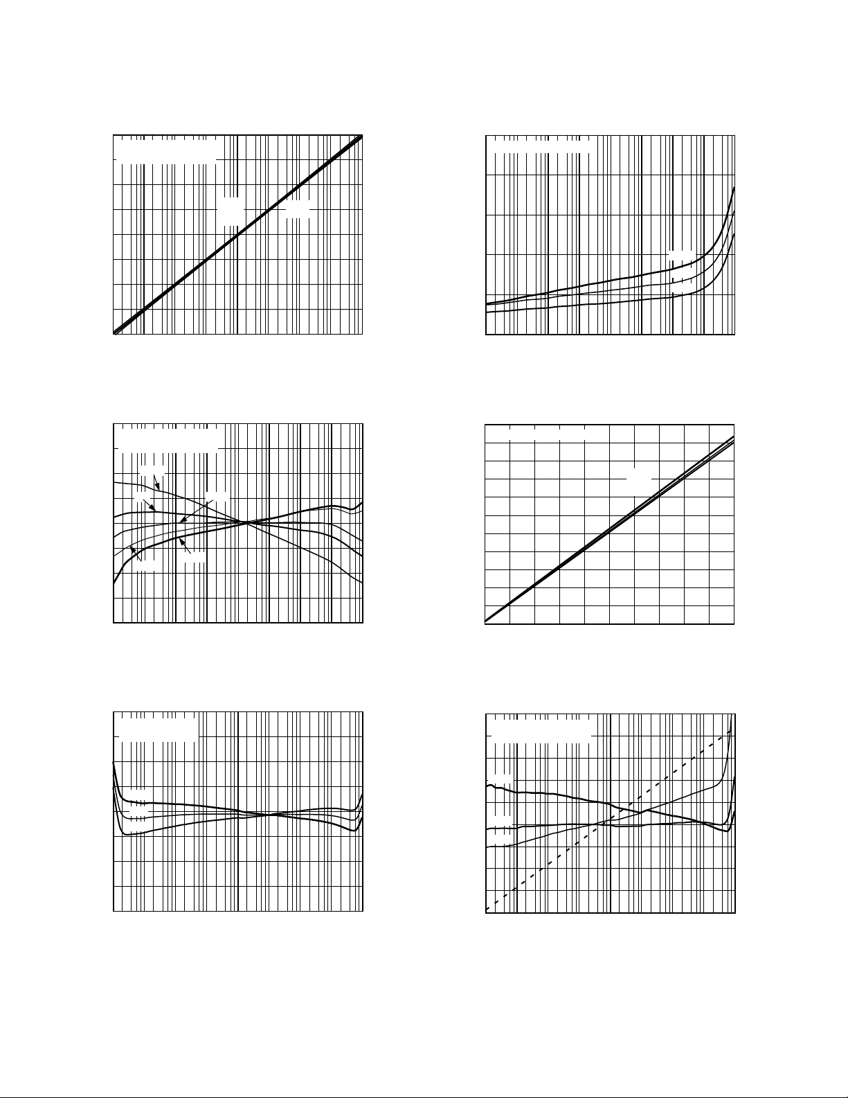
Page 5
AD8304
10
0
–10
–20
–30
–40
–50
NORMALIZED RESPONSE – dB
–60
–70
100 100M1k
100nA
10nA
1nA
10k 100k 1M 10M
FREQUENCY – Hz
1A
10A
10mA
100A
TPC 7. Small Signal AC Response, IPD to V
(5% Sine Modulation of IPD at Frequency)
100
10kHz
10
Hz
1
V rms/
0.1
1MHz
100kHz
100Hz
1kHz
1mA
LOG
10
9
8
7
6
5
4
3
WIDEBAND NOISE – mV rms
2
1
0
INPUT CURRENT – A
TPC 10. Total Wideband Noise Voltage at V
3
GAIN = 1, 2, 2.5, 5
0
AV = 5
–3
AV = 2.5
–6
NORMALIZED RESPONSE – dB
–9
A
= 2
V
LOG
AV = 1
10m100n 101n 10n 1 100 1m
vs. I
PD
0.01
IPD – A
TPC 8. Spot Noise Spectral Density at V
100
1nA
10
10nA
Hz
100nA
1
V rms/
0.1
0.01
100 10M1k
1A
10A
>100A
10k 100k 1M
FREQUENCY – Hz
TPC 9. Spot Noise Spectral Density at V
10m100n 101n 10n 1 100 1m
vs. I
LOG
vs. Frequency
LOG
PD
–12
100 100M1k
10k 100k 1M 10M
FREQUENCY – Hz
TPC 11. Small Signal Response of Buffer
10
f
= 1kHz
C
0
–10
–20
–30
–40
NORMALIZED GAIN – dB
–50
–60
–70
10 100k100
1k 10k
FREQUENCY – Hz
TPC 12. Small Signal Response of Buffer
Operating as Two-Pole Filter
REV. A
–5–
Page 6
AD8304
2.0
TA = 25C
1.5
1.0
0.5
0
–0.5
ERROR – dB (10mV/dB)
–1.0
–1.5
–2.0
100p 10m1n
MEAN + 3
MEAN – 3
10n 100n 1 10 100 1m
INPUT – A
TPC 13. Logarithmic Conformance Error
σ
Distribution (3
5
TA = 0C, 70C
4
3
2
1
0
–1
–2
ERROR – dB (10mV/dB)
–3
–4
–5
100p 10m1n
to Either Side of Mean)
MEAN + 3 @ 70C
MEAN 3 @ 0C
MEAN – 3 @ 70C
10n 100n 1 10 100 1m
INPUT – A
TPC 14. Logarithmic Conformance Error
Distribution (3
σ
to Either Side of Mean)
20
15
10
5
0
–5
DRIFT – mV
–10
REF
V
–15
–20
–25
–30
–40 90–30
TPC 16. V
MEAN + 3
MEAN – 3
–20 –10 0 10 20 40 60 80
REF
TEMPERATURE – C
Drift vs. Temperature (3σ to Either
30 50 70
Side of Mean)
3
2
1
0
–1
–2
–3
SLOPE CHANGE FROM 25C – mV/dec
–4
–5
–40 90–30
MEAN + 3
MEAN – 3
–20
–10 0 10 20 40
TEMPERATURE – C
30 50
60 80
70
TPC 17. Slope Drift vs. Temperature (3σ to Either
Side of Mean)
5
4
3
2
1
0
–1
–2
ERROR – dB (10mV/dB)
–3
–4
–5
100p 10m1n
MEAN 3 @ 85C
10n 100n 1 10 100 1m
INPUT – A
TA = 40C, 85C
MEAN 3 @40C
MEAN 3 @40C
TPC 15. Logarithmic Conformance Error
σ
Distribution (3
to Either Side of Mean)
40
30
20
10
0
–10
–20
–30
INTERCEPT CHANGE FROM 25C – pA
–40
–50
–40 90–30
MEAN + 3
MEAN – 3
–20 –10 0 10 20 40 60 80
TEMPERATURE – C
30 50 70
TPC 18. Intercept Drift vs. Temperature (3σ to
Either Side of Mean)
REV. A–6–
Page 7

AD8304
INPUT GUARD OFFSET – mV
180
0
–20 20–10
HITS
010
100
60
40
20
140
120
80
160
8
6
4
2
DRIFT – mV
0
OS
v
–2
–4
–6
–40 90–30
MEAN + 3
MEAN – 3
–20 –10 0 10 20 40 60 80
TEMPERATURE – C
30 50 70
TPC 19. Output Buffer Offset vs. Temperature
σ
to Either Side of Mean)
(3
180
160
140
120
100
HITS
80
60
40
20
0
196 204198
LOGARITHMIC SLOPE – mV/dec
200 202
TPC 20. Distribution of Logarithmic Slope, Sample 1000
160
140
120
100
80
HITS
60
40
20
0
60 14080
LOGARITHMIC INTERCEPT – pA
100 120
TPC 21. Distribution of Logarithmic Intercept,
Sample 1000
TPC 22. Distribution of Input Guard Offset Voltage
(V
– V
INPT
), Sample 1000
SUM
REV. A
–7–
Page 8

AD8304
BASIC CONCEPTS
The AD8304 uses an advanced circuit implementation that
exploits the well known logarithmic relationship between the
base-to-emitter voltage, V
, and collector current, IC, in a
BE
bipolar transistor, which is the basis of the important class of
translinear circuits*:
VV II
= log( / )
BE T C S
(1)
There are two scaling quantities in this fundamental equation, namely
the thermal voltage V
= kT/q and the saturation current IS. These
T
are of key importance in determining the slope and intercept for this
class of log amp. V
has a process-invariant value of 25.69 mV
T
at T = 25°C and varies in direct proportion to absolute temperature,
is very much a process- and device-dependent parameter,
while I
S
and is typically 10
–16
A at T = 25°C but exhibits a huge variation
over the temperature range, by a factor of about a billion.
While these variations pose challenges to the use of a transistor as
an accurate measurement device, the remarkable matching and
isothermal properties of the components in a monolithic process
can be applied to reduce them to insignificant proportions, as will
be shown. Logarithmic amplifiers based on this unique property
of the bipolar transistor are called translinear log amps to distinguish them from other Analog Devices products designed for RF
applications that use quite different principles.
The very strong temperature variation of the saturation current
I
is readily corrected using a second reference transistor, having
S
an identical variation, to stabilize the intercept. Similarly, proprietary techniques are used to ensure that the logarithmic slope is
temperature-stable. Using these principles in a carefully scaled
design, the now accurate relationship between the input current,
, applied to Pin INPT, and the voltage appearing at the inter-
I
PD
mediate output Pin VLOG is:
VV II
= log ( / )
LOG Y PD Z
10
(2)
VY is called the slope voltage (in the case of base-10 logarithms,
it is also the “volts per decade”). The fixed current I
the intercept. The scaling is chosen so that V
is called
Z
is trimmed to
Y
200 mV/decade (10 mV/dB). The intercept is positioned at
100 pA; the output voltage V
would cross zero when IPD is
LOG
of this value. However, when using a single supply the actual
must always be slightly above ground. On the other hand,
V
LOG
by using a negative supply, this voltage can actually cross zero at
the intercept value.
Using Equation 2, one can calculate the output for any value of I
PD
.
Thus, for an input current of 25 nA,
VVnApA V
==02 25 100 0 4796
. log ( / ) .
LOG
10
(3)
In practice, both the slope and intercept may be altered, to either
higher or lower values, without any significant loss of calibration
accuracy, by using one or two external resistors, often in conjunction with the trimmed 2 V voltage reference at Pin VREF.
Optical Measurements
When interpreting the current IPD in terms of optical power incident on a photodetector, it is necessary to be very clear about the
transducer properties of a biased photodiode. The units of this
transduction process are expressed as amps per watt. The parameter , called the photodiode responsivity, is often used for this
purpose. For a typical InGaAs p-i-n photodiode, the responsivity
is about 0.9 A/W.
It is also important to note that amps and watts are not usually
related in this proportional manner. In purely electrical circuits,
a current I
proportional to the square of the current (that is, I
applied to a resistive load RL results in a power
PD
2
RL). The
PD
reason for the difference in scaling for a photodiode interface is
that the current I
V
. In this case, the power dissipated within the detector
PDB
diode is simply proportional to the current I
and the proportionality of I
flows in a diode biased to a fixed voltage,
PD
(that is, IPDV
to the optical power, P
PD
PD
OPT
PDB
, is
)
preserved.
IP
=ρ
PD OPT
Accordingly, a reciprocal correspondence can be stated between
intercept current, I
IP
=ρ
ZZ
, and an equivalent “intercept power,” PZ,
Z
(4)
the
thus:
(5)
and Equation 2 may then be written as:
VV PP
= log ( / )
LOG Y OPT Z
10
(6)
For the AD8304 operating in its default mode, its IZ of 100 pA
corresponds to a P
of 110 picowatts, for a diode having a
Z
responsivity of 0.9 A/W. Thus, an optical power of 3 mW would
generate:
VVmWpW V
==02 3 110 1 487
.log( / ).
LOG
10
(7)
Note that when using the AD8304 in optical applications, the
interpretation of V
is in terms of the equivalent optical
LOG
power, the logarithmic slope remains 10 mV/dB at this output.
This can be a little confusing since a decibel change on the
optical side has a different meaning than on the electrical side.
In either case, the logarithmic slope can always be expressed in
units of mV per decade to help eliminate any confusion.
Decibel Scaling
In cases where the power levels are already expressed as so many
decibels above a reference level (in dBm, for a reference of 1 mW),
the logarithmic conversion has already been performed, and the
“log ratio” in the above expressions becomes a simple difference. One needs to be careful in assigning variable names here,
because “P” is often used to denote actual power as well as this
same power expressed in decibels, while clearly these are numerically different quantities.
Such potential misunderstandings can be avoided by using “D”
to denote decibel powers. The quantity V
must now be converted to its decibel value, V
(“volts per decade”)
Y
´ = VY/10, because
Y
there are 10 dB per decade in the context of a power measurement.
Then it can be stated that:
*For a basic discussion of the topic, see Translinear Circuits: An Historical Overview,
B. Gilbert, Analog Integrated Circuits and Signal Processing, 9, pp. 95–118, 1996.
VDDmVdB
=−
20 /
LOG OPT Z
where D
and D
OPT
is the equivalent intercept power relative to the same level.
Z
()
is the optical power in decibels above a reference level,
This convention will be used throughout this data sheet.
(8)
REV. A–8–
Page 9

AD8304
To repeat the previous example: for a reference power level of
1 mW, a P
of 3 mW would correspond to a D
OPT
of 10 log10(3) =
OPT
4.77 dBm, while the equivalent intercept power of 110 pW will
correspond to a D
VmV V
=
LOG
of –69.6 dBm; now using Equation 8:
Z
{}
=20 4 77 69 9 1 487. – (– .) .
(9)
which is in agreement with the result from Equation 7.
GENERAL STRUCTURE
The AD8304 addresses a wide variety of interfacing conditions
to meet the needs of fiber optic supervisory systems, and will also
be useful in many nonoptical applications. These notes explain
the structure of this unique translinear log amp. Figure 1 is a
simplified schematic showing the key elements.
V
PHOTODIODE
INPUT CURRENT
I
PD
INPT
C1
R1
0.5V
~10k
VSUM
0.5V
Q1
VNEG (NORMALLY GROUNDED)
200
PDB
VPDB
0.6V
V
BE1
V
BE1
V
BE2–
296mVP
I
REF
(INTERNAL)
0.5V
Q2QM
INTERCEPT AND
TEMPERATURE
COMPENSATION
(SUBTRACT AND
DIVIDE BY TK)
40A/dec
VLOG V
5k
V
BE2
ACOM
LOG
Figure 1. Simplified Schematic
The photodiode current IPD is received at input Pin INPT. The
summing voltage at this node is essentially equal to that on the
two adjacent guard pins, VSUM, due to the low offset voltage of
the ultralow bias J-FET op amp used to support the operation of
the transistor Q1, which converts the current to a logarithmic
voltage, as delineated in Equation 1. VSUM is needed to provide
the collector-emitter bias for Q1, and is internally set to 0.5 V,
using a quarter of the reference voltage of 2 V appearing on
Pin VREF.
In conventional translinear log amps, the summing node is gener-
held at ground potential, but that condition is not
ally
realized in a single-supply part. To address this, the AD8304
supports the use of an optional negative supply voltage, V
Pin VNEG. For a V
of at least –0.5 V the summing node can
N
readily
also
, at
N
be connected to ground potential. Larger negative voltages may
be used, with essentially no effect on scaling, up to a maximum
supply of 8 V between VPOS and VNEG. Note that the resistance
at the VSUM pins is approximately 10 kΩ to ground; this voltage
is not intended as a general bias source.
The input-dependent V
of Q1 is compared with the fixed VBE of
BE
a second transistor, Q2, which operates at an accurate internally
generated current, I
to be 100,000 times smaller than I
The difference between these two V
VV kTqII
– / log ( / )=
BE BE PD REF12
= 10 µA. The overall intercept is arranged
REF
, in later parts of the signal chain.
REF
values can be written as
BE
10
(10)
Thus, the uncertain and temperature-dependent saturation current,
that appears in Equation 1, has been eliminated. Next, to
I
S
eliminate the temperature variation of kT/q, this difference
voltage is applied to a processing block—essentially an analog divider
that effectively puts a variable proportional to temperature
underneath the T in Equation 10. In this same block, I
formed to the much smaller current I
defined value for V
VV II
= log ( / )
LOG Y PD Z
10
LOG
, that is,
, to provide the previously
Z
REF
is trans-
(11)
Recall that VY is 200 mV/decade and IZ is 100 pA. Internally,
this is generated first as an output current of 40 µA/decade
(2 µA/dB) applied to an internal load resistor from VLOG to
ACOM that is laser-trimmed to 5 kΩ ±1%. The slope may be
altered at this point by adding an external shunt resistor. This is
required when using the minimum supply voltage of 3.0 V,
because the span of V
range of I
amounts to 8 ⫻ 0.2 V = 1.6 V, which exceeds the
PD
for the full 160 dB (eight-decade)
LOG
internal headroom at this node. Using a shunt of 5 kΩ, this is
reduced to 800 mV, that is, the slope becomes 5 mV/dB. In
those applications needing a higher slope, the buffer can provide
voltage gain. For example, to raise the output swing to 2.4 V,
which can be accommodated by the rail-to-rail buffer when
using a 3.0 V supply, a gain of 3⫻ can be used which raises the
slope to 15 mV/dB. Slope variations implemented in these ways
do not affect the intercept. Keep in mind these measures to
address the limitations of a small positive supply voltage will not
be needed when I
can also be avoided by using a negative supply that allows V
is limited to about 1 mA maximum. They
PD
LOG
to run below ground, which will be discussed later.
Figure 1 shows how a sample of the input current is derived using
a very small monitoring transistor, Q
Q1. This is used to generate the photodiode bias, V
which varies from 0.6 V when I
, connected in parallel with
M
= 100 pA, and reverse-biases
PD
, at Pin V
PDB
PDB
,
the diode by 0.1 V (after subtracting the fixed 0.5 V at INPT)
and rises to 2.6 V at I
= 10 mA, for a net diode bias of 2 V.
PD
The driver for this output is current-limited to about 20 mA.
The system is completed by the final buffer amplifier, which is
essentially an uncommitted op amp with a rail-to-rail output
capability, a 10 MHz bandwidth, and good load-driving capabilities, and may be used to implement multipole low-pass filters,
and a voltage reference for internal use in controlling the scaling,
but that is also made available at the 2.0 V level at Pin VREF.
Figure 2 shows the ideal output V
versus IPD.
LOG
Bandwidth and Noise Considerations
The response time and wide-band noise of translinear log amps
are fundamentally a function of the signal current I
bandwidth becomes progressively lower as I
PD
. The
PD
is reduced,
largely due to the effects of junction capacitances in Q1. This is
easily understood by noting that the transconductance (g
bipolar transistor is a linear function of collector current, I
(hence, translinear), which in this case is just I
PD
) of a
m
C
. The corre-
,
sponding incremental emitter resistance is:
==
e
g
m
qI
PD
(12)
kT
1
r
Basically, this resistance and the capacitance CJ of the transistor
generate a time constant of r
and thus a corresponding low-pass
eCJ
corner frequency of:
qI
2=π
PD
kTC
j
(13)
f
dB
3
showing the proportionality of bandwidth to current.
REV. A
–9–
Page 10

AD8304
1.6
1.2
– V
0.8
LOG
V
0.4
0
100p 10m1n 10n 100n 1 10 100 1m
Figure 2. Ideal Form of V
INPUT – A
LOG
vs. I
PD
Using a value of 0.3 pF for CJ evaluates to 20 MHz/mA. Therefore, the minimum bandwidth at I
= 100 pA would be 2 kHz.
PD
While this simple model is useful in making a point, it excludes
other effects that limit its usefulness. For example, the network
R1, C1 in Figure 1, which is necessary to stabilize the system over
the full range of currents, affects bandwidth at all values of I
PD
.
Later signal processing blocks also limit the maximum value.
TPC 7 shows ac response curves for the AD8304 at eight representative currents of 100 pA to 10 mA, using R
C
= 1000 pF. The values for R1 and C1 ensure stability over
1
= 750 Ω and
1
the full 160 dB dynamic range. More optimal values may be used
for smaller subranges. A certain amount of experimental trial and
error may be necessary to select the optimum input network
component values for a given application.
Turning now to the noise performance of a translinear log amp,
the relationship between I
S
, associated with the VBE of Q1, evaluates to the following:
NSD
S
where S
14 7.
=
NSD
I
PD
is nV/Hz, IPD is expressed in microamps and TA= 25°C.
NSD
For an input of 1 nA, S
and the voltage noise spectral density,
PD
evaluates to almost 0.5 µV/√Hz; assum-
NSD
(14)
ing a 20 kHz bandwidth at this current, the integrated noise
voltage is 70 µV rms. However, the calculation is not complete.
The basic scaling of the V
is approximately 3 mV/dB; translated
BE
to 10 mV/dB, the noise predicted by Equation 14 must be multiplied by approximately 3.33. The additive noise effects associated
with the reference transistor, Q2, and the temperature compensation circuitry must also be included. The final voltage noise
spectral density presented at the VLOG Pin varies inversely with
, but not as simple as square root. TPCS8 and 9 show the
I
PD
measured noise spectral density versus frequency at the VLOG
output, for the same nine-decade spaced values of I
PD
.
Chip Enable
The AD8304 may be powered down by taking the PWDN Pin
to a high logic level. The residual supply current in the disabled
mode is typically 60 µA.
USING THE AD8304
The basic connections (Figure 3) include a 2.5:1 attenuator in
the feedback path around the buffer. This increases the basic slope
of 10 mV/dB at the VLOG Pin to 25 mV/dB at V
. For the
OUT
full dynamic range of 160 dB (80 dB optical), the output swing
is thus 4.0 V, which can be accommodated by the rail-to-rail
output stage when using the recommended 5 V supply.
The capacitor from VLOG to ground forms an optional singlepole low-pass filter. Since the resistance at this pin is trimmed
to 5 kΩ, an accurate time constant can be realized. For example, with C
= 10 nF, the –3 dB corner frequency is
FLT
3.2 kHz. Such filtering is useful in minimizing the output noise,
particularly when I
is small. Multipole filters are more effec-
PD
tive in reducing noise, and are discussed below. A capacitor
between VSUM and ground is essential for minimizing the
noise on this node. When the bias voltage at either VPDB or
VREF is not needed these pins should be left unconnected.
Slope and Intercept Adjustments
The choice of slope and intercept depends on the application.
The versatility of the AD8304 permits optimal choices to be
made in two common situations. First, it allows an input current
range of less than the full 160 dB to use the available voltage span
at the output. Second, it allows this output voltage range to be
optimally positioned to fit the input capacity of a subsequent
ADC. In special applications, very high slopes, such as 1 V/dec,
allow small subranges of I
to be covered at high sensitivity.
PD
The slope can be lowered without limit by the addition of a
shunt resistor, R
, from VLOG to ground. Since the resistance
S
at this pin is trimmed to 5 kΩ, the accuracy of the modified
slope will depend on the external resistor. It is calculated using:
VR
V
Y
I
PD
C1
1nF
10nF
R1
750
NC = NO CONNECT
YS
=
Rk
+'5Ω
S
VPDB
NC
VSUM
3
INPT
4
VSUM
5
VNEG
VPS2 PWDN VPS1
10
PDB BIAS VREF
1
2 12
~10k
TEMPERATURE
COMPENSATION
ACOM
0.5V
14
5k
VOUT
VLOG
BFIN
BFNG
11
V
P
7
VREF
200mV/DEC
8
9
13
V
500mV/DEC
CFLT
RB
10k
RA
15k
OUT
(15)
Figure 3. Basic Connections (RA, RB, CFLT are
optional; R1 and C1 are the default values)
For example, using RS= 3 kΩ, the slope is lowered to 75 mV per
decade or 3.75 mV/dB. Table I provides a selection of suitable
values for R
and the resulting slopes.
S
Table I. Examples of Lowering the Slope
RS (k)V
(mV/dec)
Y
375
5 100
15 150
REV. A–10–
Page 11

AD8304
In addition to uses in filter and comparator functions, the buffer
amplifier provides the means to adjust both the slope and intercept, which require a minimal number of external components.
The high input impedance at BFIN, low input offset voltage,
large output swing, and wide bandwidth of this amplifier permit
numerous transformations of the basic V
signal, using stan-
LOG
dard op amp circuit practices. For example, it has been noted
that to raise the gain of the buffer, and therefore the slope, a
feedback attenuator, R
and RB in Figure 3, should be inserted
A
between VLOG and the inverting input Pin BFNG.
A wide range of gains may be used and the resistor magnitudes
are not critical; their parallel sum should be about equal to the
net source resistance at the noninverting input. When high gains
are used, the output dynamic range will be reduced; for maximum swing of 4.8 V, it will amount to simply 4.8 V/V
decades.
Y
Thus, using a ratio of 3⫻, to set up a slope 30 mV/dB (600 mV/
decade), eight decades can be handled, while with a ratio of 5⫻,
which sets up a slope of 50 mV/dB (1 V/decade), the dynamic
range is 4.8 decades, or 96 dB. When using a lower positive
supply voltage, the calculation proceeds in the same way,
remembering to first subtract 0.2 V to allow for 0.1 V upper and
lower headroom in the output swing.
Alteration of the logarithmic intercept is only slightly more tricky.
First note that it will rarely be necessary to lower the intercept
below a value of 100 pA, since this merely raises all output voltages further above ground. However, where this is required, the
first step is to raise the voltage V
by connecting a resistor, RZ,
LOG
from VLOG to VREF (2 V) as shown in Figure 4.
V
VLOG
BFIN
BFNG
7
8
9
13
P
VREF
RA
RZ
RB
V
OUT
I
PD
VPDB
6
NC
VSUM
3
INPT
4
5
VSUM
VNEG
C1
1nF
10nF
R1
750
NC = NO CONNECT
VPS2 PWDN VPS1
10
PDB BIAS VREF
1
2 12
~10k
TEMPERATURE
COMPENSATION
ACOM
0.5V
14
5k
VOUT
11
Figure 4. Method for Lowering the Intercept
This has the effect of elevating V
ing the slope to some extent because of the shunt effect of R
for small inputs while lower-
LOG
Z
on the 5 kΩ output resistance. Then, if necessary, the slope may
be increased as before, using a feedback attenuator around the
buffer. Table II lists some examples of lowering the intercept
combined with various slope variations.
Table II. Examples of Lowering the Intercept
VY (mV/decade) IZ (pA) RA (k)RB (k)RZ (k)
200 1 20.0 100 25
200 10 10.0 100 50
200 50 3.01 100 165
300 1 10.0 12.4 25
300 10 8.06 12.4 50
300 50 6.65 12.4 165
400 1 11.5 8.2 25
400 10 9.76 8.2 50
400 50 8.66 8.2 165
500 1 16.5 8.2 25
500 10 14.3 8.2 50
500 50 13.0 8.2 165
Equations for use with Table II:
VGV
OUT Y
=×
R
Z
RR
+
Z LOG
I
PD
log
×
10
V
+×
I
Z
REF
R
RR
LOG Z
LOG
+
where
R
G
A
=+ = Ω15and
R
B
Rk
LOG
Generally, it will be useful to raise the intercept. Keep in mind
that this moves the V
line in Figure 2 to the right, lowering all
LOG
output values. Figure 5 shows how this is achieved. The feedback
resistors, R
a third resistor, R
and RB, around the buffer are now augmented with
A
, placed between the Pins BFNG and VREF.
Z
This raises the zero-signal voltage on BFNG, which has the effect
of pushing V
lower. Note that the addition of this resistor also
OUT
alters the feedback ratio. However, this is readily compensated
in the design of the network. Table III lists the resistor values
for representative intercepts.
Table III. Examples of Raising the Intercept
VY (mV/decade) IZ (nA) RA (k)RB (k)RC(k)
300 10 7.5 37.4 24.9
300 100 8.25 130 18.2
400 10 10 16.5 25.5
400 100 9.76 25.5 16.2
400 500 9.76 36.5 13.3
500 10 12.4 12.4 24.9
500 100 12.4 16.5 16.5
500 500 11.5 20.0 12.4
Equations for use with Table III:
VGV
=×
OUT Y
log –
I
PD
V
10
I
REF
Z
RR
AB
×
RR R
AB C
+
where
REV. A
–11–
R
G
=+ =
A
1 and
RR
BC
RR
AB
RR
×
AB
RR
+
AB
Page 12

AD8304
I
PD
6
NC
3
4
C1
5
1nF
10nF
R1
750
NC = NO CONNECT
VPS2 PWDN VPS1
10
PDB BIAS VREF
VPDB
VSUM
INPT
VSUM
1
VNEG
2 12
~10k
TEMPERATURE
COMPENSATION
ACOM
V
P
Using the Adaptive Bias
For most photodiode applications, the placement of the anode
somewhat above ground is acceptable, as long as the positive
VREF
7
0.5V
VLOG
8
5k
BFIN
BFNG
13
14
VOUT
11
RC
9
RA
RB
V
OUT
bias on the cathode is adequate to support the peak current for a
particular diode, limited mainly by its series resistance. To address
this matter, the AD8304 provides for the diode a bias that varies
linearly with the current. This voltage appears at Pin VPDB, and
varies from 0.6 V (reverse-biasing the diode by 0.1 V) for I
100 pA and rises to 2.6 V (for a diode bias of 1 V) at I
PD
=
PD
= 10 mA.
This results in a constant internal junction bias of 0.1 V when the
series resistance of the photodiode is 200 Ω. For optical power
measurements over a wide dynamic range the adaptive biasing
function will be valuable in minimizing dark current while preventing the loss of photodiode bias at high currents. Use of the
adaptive bias feature is shown in Figure 7.
Figure 5. Method for Raising the Intercept
Low Supply Slope and Intercept Adjustment
When using the device with a positive supply less than 4 V, it is
necessary to reduce the slope and intercept at the VLOG Pin in
order to preserve good log conformance over the entire 160 dB
operating range. The voltage at the VLOG Pin is generated by
an internal current source with an output current of 40 µA/decade
feeding the internal laser-trimmed output resistance of 5 kΩ. When
the voltage at the VLOG Pin exceeds V
– 2.3 V, the current
P
source ceases to respond linearly to logarithmic increases in current.
This headroom issue can be avoided by reducing the logarithmic
slope and intercept at the VLOG Pin. This is accomplished by
connecting an external resistor R
in combination with an intercept lowering resistor R
from the VLOG Pin to ground
S
. The values
Z
shown in Figure 6 illustrate a good solution for a 3.0 V positive
supply. The resulting logarithmic slope measured at VLOG is
62.5 mV/decade with a new intercept of 57 fA. The original
logarithmic slope of 200 mV/decade can be recovered using voltage
gain on the internal buffer amplifier.
V
I
PD
VPDB
6
NC
VSUM
3
INPT
4
5
VSUM
C1
1nF
10nF
R1
750
NC = NO CONNECT
VPS2 PWDN VPS1
10
PDB BIAS VREF
1
VNEG
2 12
~10k
TEMPERATURE
COMPENSATION
ACOM
14
0.5V
5k
VOUT
11
VREF
VLOG
BFIN
BFNG
P
7
RZ
15.4k
2.67k
8
9
62.5mV/DEC
13
RA
4.98k
RS
RB
2.26k
V
OUT
Figure 6. Recommended Low Supply Application Circuit
V
VLOG
BFIN
BFNG
P
VREF
7
CFILT
8
9
RB
13
RA
V
OUT
CPB
C1
1nF
10nF
R1
750
VPDB
I
PD
VPS2 PWDN VPS1
10
PDB BIAS VREF
6
3
4
5
VSUM
INPT
VSUM
VNEG
1
~10k
TEMPERATURE
COMPENSATION
ACOM
2 12
0.5V
14
VOUT
5k
11
Figure 7. Using the Adaptive Biasing
Capacitor CPB, between the photodiode cathode at Pin VPDB
and ground, is included to lower the impedance at this node and
thereby improve the high frequency accuracy at those current
levels where the AD8304 bandwidth is high. It also ensures an
HF path for any high frequency modulation on the optical signal
which might not otherwise be accurately averaged. It will not be
necessary in all cases, and experimentation may be required to find
an optimum value.
Changing the Voltage at the Summing Node
The default value of VSUM is determined by using a quarter of
VREF (2 V). This may be altered by applying an independent voltage source to VSUM, or by adding an external resistive divider
from VREF to VSUM. This network will operate in parallel with
the internal divider (40 kΩ and 13.3 kΩ), and the choice of external
resistors should take this into account. In practice, the total
resistance of the added string may be as low as 10 kΩ (consuming
400 µA from VREF). Low values of VSUM and thus V
Figure 13) are not advised when large values of I
PD
(see
CE
are expected.
Implementing Low-Pass Filters
Noise, leading to uncertainty in an observed value, is inherent to
all measurement systems. Translinear log amps exhibit significant
amounts of noise for reasons stated above, and are more troublesome at low current levels. The standard way of addressing this
problem is to average the measurement over an appropriate time
interval. This can be achieved in the digital domain, in post-ADC
DSP, or in analog form using a variety of low-pass structures.
REV. A–12–
Page 13

The use of a capacitor at the VLOG Pin to create a single-pole
filter has already been mentioned. The small added cost of the few
external components needed to realize a multipole filter is often
justified in a high performance measurement system. Figure 8
shows a Sallen-Key filter structure. Here, the resistor needed at
the front of the network is provided entirely by the accurate 5 kΩ
present at the VLOG output; R
will have a similar value. The corner
B
frequency and Q (damping factor) are determined by the capacitors
C
and CB and the gain G = (RA+ RB)/RB. A suggested starting
A
point for choosing these components using various gains is provided in Table IV; the values shown are for a 1 kHz corner (also
see TPC 12). This frequency can be increased or decreased by
scaling the capacitor values. Note that R
C
should not deviate from the suggested values to maintain the
A/CB
, G, and the capacitor ratio
D
shape of the ac amplitude response and pulse overshoot provided
by the values shown in this table. In all cases, the roll-off rate above
the corner is 40 dB/dec.
V
11
BFIN
BFNG
7
8
9
13
P
VREF
VLOG
CA
RD
RB
CB
RA
V
OUT
I
PD
VPDB
6
NC
VSUM
3
INPT
4
10nF
5
VSUM
C1
1nF
R1
750k
NC = NO CONNECT
VPS2 PWDN VPS1
10
PDB BIAS VREF
1
VNEG
2 12
~10k
TEMPERATURE
COMPENSATION
ACOM
14
0.5V
5k
VOUT
Figure 8. Two-Pole Low-Pass Filter
Table IV. Two-Pole Filter Parameters for 1 kHz Cutoff
Frequency*
R
R
A
B
V
Y
R
D
C
C
A
B
(k)(k)G (V/decade) (k) (nF) (nF)
0 open 1 0.2 11.3 12 12
10 10 2 0.4 6.02 33 22
12 8 2.5 0.5 12.1 33 18
24 6 5 1.0 10.0 33 18
The corner frequency can be adjusted by scaling capacitors CA and CB. For
example, to reduce the corner frequency to 100 Hz, raise the values of CA and
CB by 10 ⫻.
*See TPC 12.
Operation in Comparator Modes
In certain applications, the need may arise to generate a logical
output when the input current has reached a certain value. This
can be easily addressed by using a fraction of the voltage reference to provide the setpoint (threshold) and using the buffer
without feedback in a comparator mode, as illustrated in Figure 9.
Since V
runs from ground up to 1.6 V maximum, the 2 V
LOG
reference is more than adequate to cover the full dynamic range
. Note that the threshold for an increasing IPD is unchanged,
of I
PD
while the release point for decreasing currents is 5 dB below
this. Raising R
may be increased using a lower value for R
to 5 MΩ reduces the hysteresis to 0.5 dB, or it
H
.
H
AD8304
V
VPS2 PWDN VPS1
I
PD
VPDB
6
NC
VSUM
3
INPT
4
5
VSUM
C1
1nF
10nF
R1
750
NC = NO CONNECT
10
PDB BIAS VREF
1
VNEG
2 12
~10k
TEMPERATURE
COMPENSATION
ACOM
0.5V
5k
14
VOUT
Figure 9. Using the Buffer as a Comparator
Using a Negative Supply
Most applications of the AD8304 will require only a single supply
of 3.0 V to 5.5 V. However, to provide further versatility, dual
supplies may be employed, as illustrated in Figure 10.
The use of a negative supply, V
, allows the summing node to
N
be placed exactly at ground level, because the input transistor
(Q1 in Figure 1) will have a negative bias on its emitter. V
be as small as –0.5 V, making the V
the same as for the default
CE
case. This bias need not be accurate, and a poorly defined source
can be used.
A larger supply of up to –5V may be used. The effect on scaling
is minor. It merely moves the intercept by ~0.01 dB/V. Accordingly, an uncertainty of 0.2 V in V
would result in a negligible
N
error of 0.002 dB. The slope is unaffected by V
earity will be degraded at the extremes of the dynamic range as
indicated in Figure 11. The bias current, buffer output (and its
load) current, and the full I
all have to be absorbed by this
PD
negative supply, and its supply capacity must be ensured for the
maximum current condition.
VPS2 PWDN VPS1
I
PD
VPDB
6
NC
VSUM
3
INPT
4
5
VSUM
V
C1
1nF
R1
750
NC = NO CONNECT
10
PDB BIAS VREF
1
VNEG
N (–0.5V TO –3V)
2 12
~10k
TEMPERATURE
COMPENSATION
ACOM
0.5V
5k
14
VOUT
Figure 10. Using a Negative Supply
With the summing node at ground, the AD8304 may now be used
as a voltage-input log amp, simply by inserting a suitably scaled
resistor from the voltage source to the INPT Pin. The logarithmic accuracy for small voltages is limited by the offset of the JFET
op amp, appearing between this pin and VSUM.
The use of a negative supply also allows the output to swing below
ground, thereby allowing the intercept to correspond to a midrange
value of I
. However, the voltage V
PD
remains referenced to the
LOG
P
VREF
7
VLOG
8
BFIN
9
BFNG
13
RH
11
. The log lin-
N
V
P
7
VREF
VLOG
8
BFIN
9
BFNG
13
11
RB
V
OUT
N
V
OUT
RG
RA
may
RA
REV. A
–13–
Page 14

AD8304
ACOM Pin, and does not normally go negative with regard to this
pin, but is free to do so. Therefore, a resistor from VLOG to the
negative supply can lower V
, thus raising the intercept. A more
LOG
accurate method for repositioning the intercept is described below.
2.0
1.5
1.0
0.5
0
–0.5
ERROR – dB (10mV/dB)
–1.0
–1.5
–2.0
100p 10m1n 10n 100n 1 10 100 1m
WITHOUT INTERCEPT ADJUST
WITH INTERCEPT ADJUST
INPUT – A
V
= 0
NEG
V
= –0.5
NEG
V
= –3
NEG
Figure 11. Log Conformance (Linearity) vs. IPD for
Various Negative Supplies
APPLICATIONS
The AD8304 incorporates features that improve its usefulness in
both fiber optic supervisory applications and in more general ones.
To aid in the exploration of these possibilities, a SPICE macromodel is provided and a versatile evaluation board is available.
The macromodel is shown in generalized schematic form (and thus
is independent of variations in SPICE programs) in Figure 12.
Q1, QM, and Q2 (here made equal in size) correspond to the
identical transistors in Figure 1. The model parameters for these
transistors are not critical; the default model provided in SPICE
libraries will be satisfactory. However, the AD8304 employs
compensation techniques to reduce errors caused by junction
resistances (notably, RB and RE) at high input currents. Therefore, it is advisable to set these to zero. While this will not model
the AD8304 precisely, it is safer than using possibly high default
values for these parameters. The low current model parameters
may also need consideration. Note that no attempt is made to
capture either dynamic behavior or the effects of temperature in this
simple macromodel; scaling is correct for 27°C.
E2
5
I1
IPD
IN
C1
I1
C1
E1
V1
Q1
I2
Q2
I3
Q3
.MODEL
E2
E3
E4
V2
R1
C2
R2
RL
V1
V
+
Q1
0
IN
2
1
IN
0
3
0
4
NPN
5
6
7
8
8
9
9
VLOG
1
3k
IN
DC
0
1.0N
0
IN
0
0.5
2
0
3
1
3
0
4
316.2
4
0
NPN
0
POLY (2)
0
POLY (2)
0
6 5 100K
7
0.8
9
100
0
163P
VLOG
4.9K
0
1000K
I1
2
3
Q2
1A
1
NPN
NPN
NPN
2 3 1 0 0, 0, 0, 0, 1
4 3 7 0 0, 0, 0, 0, 1
I2
4
Q3
3K
E3
E4
100k
6
Figure 12. Basic Macromodel
V2
R2
R1
7
+
V
C2
VLOG
RL
REV. A–14–
Page 15

AD8304
Summing Node at Ground and Voltage Inputs
A negative supply may be used to reposition the input node at
ground potential. A voltage as small as –0.5 V is sufficient. Figure 13
shows the use of this feature. An input current of up to 10 mA is
supported.
This connection mode will be useful in cases where the source is a
positive voltage V
photodiodes, or other “perfect” current sources. R
referenced to ground, rather than for use with
SIG
scales the
IN
input current and should be chosen to optimally position the range
of I
, or provide a very high input resistance, thus minimizing
PD
the loading of the signal source. For example, assume a voltage
source that spans the four-decade range from 100 mV to 1 kV and
is desired to maximize R
. When set to 1 GΩ, IPD spans the range
IN
100 pA to 1 mA. Using a value of 10 MΩ, the same four decades
of input voltage would span the central current range of 10 nA
to 100 mA.
Smaller input voltages can be measured accurately when aided by
a small offset-nulling voltage applied to VSUM. The optional
network shown in Figure 13 provides more than ±20 mV for
this purpose.
V
BFIN
BFNG
7
8
9
13
P
VREF
VLOG
RB
RA
V
OUT
AD8304
VPDB
6
NC
VSUM
RIN
V
P
NC = NO CONNECT
3
4
I
PD
VSUM
5
V
SIG
1k
V
LOW
10k
VPS2 PWDN VPS1
10
PDB BIAS VREF
INPT
1
VNEG
V
~10k
N
2 12
TEMPERATURE
COMPENSATION
14
ACOM
0.5V
5k
VOUT
11
Figure 13. Using a Negative Supply and Placing VSUM at
Ground Permits Voltage-Mode Inputs
The minimum voltage that can be accurately measured is then
limited only by the drift in the input offset of the AD8304. The
specifications show the maximum spread over the full temperature and supply range. Over a limited temperature range, and with
a regulated supply, the offset drift will be lower; in this situation,
processing of inputs down to 5 mV is practicable.
The input system of the AD8304 is quasi-differential, so VSUM
can be placed at an arbitrary reference level V
, over a wide
LOW
range, and used as the “signal LO” of the source. For example,
using V
= 5 V and VN = –3 V, V
P
can be any voltage within
LOW
a ±2.5 V range.
Providing Negative Outputs and Rescaling
As noted, the AD8304 allows the buffer to drive a load to negative
voltages with respect to ACOM, the analog common pin, which
is grounded. A negative supply capable of supporting the input
current I
must be used, the fraction of quiescent bias that flows
PD
out of the VNEG Pin, and the load current at VLOG. For the
example shown in Figure 14, this totals less than 20 mA when
driving a 1 kΩ load as far as –4V.
The use of a much larger value for the intercept may be useful in
certain situations. In this example, it has been moved up four
decades, from the default value of 100 pA to the center of the full
eight-decade range at 1 mA. Using a voltage input as described
above, this corresponds to an altered voltage-mode intercept, V
which would be 1 V for R
= 1 MΩ. To take full advantage of the
IN
,
Z
larger output swing, the gain of the buffer has been increased to
4.53, resulting in a scaling of 900 mV/decade and a full-scale
output of ±3.6 V.
V
BFIN
BFNG
7
8
9
13
P
VREF
VLOG
RB
22.6k
V
OUT
RC
12.4k
RA
13.3k
RL
1k
NC
RIN
I
PD
V
SIG
1k
V
P
10k
NC = NO CONNECT
VPS2 PWDN VPS1
AD8304
VPDB
6
VSUM
3
INPT
4
VSUM
5
V
LOW
10
PDB BIAS VREF
~10k
TEMPERATURE
COMPENSATION
1
VNEG
ACOM
V
N
2 12
0.5V
14
VOUT
5k
11
Figure 14. Using a Negative Supply to Allow the
Output to Swing Below Ground
Inverting the Slope
The buffer is essentially an uncommitted op amp that can be used
to support the operation of the AD8304 in a variety of ways. It
can be completely disconnected from the signal chain when not
needed. Figure 15 shows its use as an inverting amplifier; this
changes the polarity of the slope. The output can either be
repositioned to all positive values by applying a fraction of V
REF
to the BFIN Pin, or range negative when using a negative supply.
The full design for a practical application is left undefined in this
brief illustration, but a few cases will be discussed.
For example, suppose we need a slope of –30 mV/dB; this requires
the gain to be three. Since V
5kΩ, R
must be 15 kΩ. In cases where a small negative supply
B
exhibits a source resistance of
LOG
is available, the output voltage can swing below ground, and the
BFIN Pin may be grounded. But a negative slope is still possible
when only a single supply is used; a positive offset, V
, is applied
OFS
to this pin, as indicated in Figure 15. In general, the resulting
output voltage can be expressed as:
R
V
OUT
B
=
V
Y
k
5
Ω
I
PD
×
10
V
+– log
OFS
I
Z
(16)
REV. A
–15–
Page 16

AD8304
V
P
VPS2 PWDN VPS1
AD8304
I
PD
VPDB
6
NC
VSUM
3
INPT
4
5
VSUM
V
C1
1nF
10nF
R1
750
NC = NO CONNECT
10
PDB BIAS VREF
1
VNEG
N
(–0.5V TO –3V)
2
~10k
TEMPERATURE
COMPENSATION
ACOM
14
Figure 15. Using the Buffer to Invert the Polarity
of the Slope
When the gain is set to 13 (RB= 5 kΩ) the 2 V V
directly to BFIN, in which case the starting point for the output
response is at 4 V. However, since the slope in this case is only
–0.2 V/decade, the full current range will only take the output
0.5V
12
5k
VOUT
7
8
BFIN
9
BFNG
13
11
can be tied
REF
VREF
VLOG
V
OFS
RB
V
OUT
down by 1.6 V. Clearly, a higher slope (or gain) is desirable, in
which case V
the output at low currents. If V
should be set to a smaller voltage to avoid railing
OFS
= 1.2 V and G = 33, VOUT
OFS
now starts at 4.8 V and falls through this same voltage toward
ground with a slope of –0.6 V per decade, spanning the full
range of I
PD
.
Programmable Level Comparator with Hysteresis
The buffer amplifier and reference voltage permit a calibrated
level detector to be realized. Figure 16 shows the use of a 10-bit
MDAC to control the setpoint to within 0.1 dB of an exact value
over the 100 dB range of 1 nA ≤ I
≤ 100 µA when the full-
PD
scale output of the MDAC is equal to that of its reference. The
2 V V
also sets the minimum value of V
REF
to 0.2 V, correspond-
SPT
ing to an input of 1 nA. Since 100 dB at the VLOG interface
corresponds to a 1 V span, the resistor network is calculated to
provide a maximum V
10% of V
REF
.
of 1.2 V while adding the required
SPT
In this example, the hysteresis range is arranged to be 0.1 dB,
(1 mV at VLOG) when using a 5 V supply. This will usually be
adequate to prevent noise that causes the comparator output to
thrash. That risk can be reduced further by using a low-pass filtering
capacitor at V
(shown dotted) to decrease the noise bandwidth.
LOG
I
PD
NC
1nF
10nF
750
NC = NO CONNECT
I
SRC
NC
25k
VPS2 PWDN VPS1
10
2 12
AD8304
PDB BIAS VREF
~10k
INPT
TEMPERATURE
COMPENSATION
1
VNEG
ACOM
0.5V
14
VOUT
6
3
4
5
VPDB
VSUM
VSUM
Figure 16. Calibrated Level Comparator
VPS2 PWDN VPS1
AD8304
VPDB
6
VSUM
3
INPT
4
VSUM
5
10
PDB BIAS VREF
2 12
~10k
TEMPERATURE
COMPENSATION
0.5V
5k
11
5k
VLOG
BFIN
BFNG
BFNG
BFIN
13
V
7
8
9
P
VREF
V
SPT
RH
V
7
8
9
13
50M
V
P
VREF
VLOG
49.9k
100k
OUT
VOUT
VOUT
VREF
MDAC
VREF
MDAC
C2
1nF
VNEG
1k
NC = NO CONNECT
VN (–0.5V TO –5V)
1
ACOM
14
VOUT
11
Figure 17. Multidecade Current Source
C1
10nF
100k
REV. A–16–
Page 17

AD8304
Programmable Multidecade Current Source
The AD8304 supports a wide variety of general (nonoptical)
applications. For example, the need frequently arises in test
equipment to provide an accurate current that can be varied over
many decades. This can be achieved using a logarithmic amplifier
as the measuring device in an inverse function loop, as illustrated
in Figure 16. This circuit generates the current:
V
02/.
()
IpA
=×
100 10
SRC
SPT
(17)
The principle is as follows. The current in QA is forced to supply
a certain I
V
LOG
by measuring the error between a setpoint V
PD
, and nulling this error by integration. This is performed by
SPT
and
the internal op amp and capacitor C1, with a time constant formed
with the internal 5 kΩ resistor. The choice of C1 in this example
ensures loop stability over the full eight-decade range of output
currents; C2 reduces phase lag. The system is completed with a
10-bit MDAC using V
as its reference, whose output is scaled
REF
to 1.6 V FS by R1 and R2 (whose parallel sum is also 5 kΩ).
Transistor QA may be a single bipolar device, which will result in
a small alpha error in I
(the current is monitored in the emitter
SRC
branch), or a Darlington pair or an MOS device, either of which
ensure a negligible difference between I
PD
and I
. In this example,
SRC
the bipolar pair is used. The output voltage compliance is determined by the collector breakdown voltage of these transistors,
while the minimum voltage depends on where VSUM is placed.
Optional components could be added to put this node and VNEG
at a low enough bias to allow the voltage to go slightly below ground.
Many variations of this basic circuit are possible. For example, the
current can be continuously controlled by a simple voltage, or
by a second current. Larger output currents can be controlled by
setting V
to zero and using a current shunt divider.
SUM
Characterization Setups and Methods
During the primary characterization of the AD8304, the device
was treated as a high precision current-in logarithmic amplifier
(converter). Rather than attempting to accurately generate photocurrents by illuminating a photodiode, precision current sources,
like the Keithley 236, were used as input sources. Great care was
taken when applying the low level input currents. The triax output
of the current source was used with the guard connected to VSUM
at the characterization board. On the board the input trace was
guarded by connecting adjacent traces and a portion of an internal
copper layer to the VSUM Pins. One obvious reason for the care
was leakage current. With 0.5 V as the nominal bias on the
INPT Pin, a resistance of 50 GΩ to ground would cause 10 pA
of leakage, or about one decibel of error at the low end of the
measurement range. Additionally, the high output resistance of
the current source and the long signal cable lengths commonly
needed in characterization make a good receiver for 60 Hz emissions. Good guarding techniques help to reduce the pickup of
unwanted signals.
TRIAX
CONNECTOR*
PWDN VNEG VPOS
VOUT
AD8304
KEITHLEY 236
*SIGNAL: INPT;
GUARD: VSUM;
SHIELD: GROUND
INPT
CHARACTERIZATION
BOARD
VSUM VPDB VREF
DC MATRIX, DC SUPPLIES, DMM
BFIN
VLOG
RIBBON
CABLE
Figure 18. Primary Characterization Setup
The primary characterization setup shown in Figure 18 is used to
measure the static performance, logarithmic conformance, slope
and intercept, buffer offset and V
drift with temperature, and
REF
the performance of the VPDB Pin functions. For the dynamic tests,
such as noise and bandwidth, more specialized setups are used.
HP 3577A
NETWORK
ANALYZER
+IN
AD8138
EVALUATION
BOARD
OUTPUT INPUT INPUTA
B
POWER
A
SPLITTER
INPUTB
1
2
3
4
5
6
7
AD8304
VNEG
PWDN
VSUM
INPT
VSUM
VPDB
VREF
ACOM
BFNG
VPS1
VOUT
VPS2
BFIN
VLOG
14
13
12
11
10
9
8
49.9
+V
0.1F
S
Figure 19. Configuration for Buffer Amplifier
Bandwidth Measurement
Figure 19 shows the configuration used to measure the buffer
amplifier bandwidth. The AD8138 Evaluation Board provides a
dc offset at the buffer input, allowing measurement in single-supply
mode. The network analyzer input impedance was set to 1 MΩ.
REV. A
–17–
Page 18

AD8304
HP 3577A
NETWORK
ANALYZER
OUTPUT INPUT INPUTA
POWER
SPLITTER
+IN
AD8138
EVALUATION
BOARD
INPUTB
B
A
R1
750
1nF
1
2
3
4
5
6
7
AD8304
VNEG
PWDN
VSUM
INPT
VSUM
VPDB
VREF
ACOM
BFNG
VPS1
VOUT
VPS2
BFIN
VLOG
14
13
12
11
10
9
8
+V
0.1F
S
Figure 20. Configuration for Logarithmic
Amplifier Bandwidth Measurement
The setup shown in Figure 20 was used for frequency response
measurements of the logarithmic amplifier section. In this configuration, the AD8138 output was offset to 1.5 V and R1 was
adjusted to provide the appropriate operating current. The
buffer amplifier was then used; still any capacitance added at
the VLOG Pin during measurement would form a filter with the
on-chip 5 kΩ resistor.
The configuration illustrated in Figure 21 measures the device
noise. Batteries provide both the supply and the input signal to
remove the supplies as a possible noise source and to reduce
ground loop effects. The AD8304 Evaluation Board and the
current setting resistors are mounted in closed aluminum enclosures to provide additional shielding to external noise sources.
HP 89410A
SOURCE TRIGGER
CHANNEL
1
CHANNEL
2
AD8304
ALKALINE
D CELL
R1
750
1nF
1
2
3
4
5
6
7
VNEG
PWDN
VSUM
INPT
VSUM
VPDB
VREF
ACOM
BFNG
VPS1
VOUT
VPS2
BFIN
VLOG
14
13
12
11
10
9
8
ALKALINE
D CELL
Figure 21. Configuration for Noise Spectral
Density Measurement
Evaluation Board
An evaluation board is available for the AD8304, the schematic
for which is shown in Figure 22, and the two board sides are
shown in Figure 23 and Figure 24. It can be configured for a wide
variety of experiments. The board is factory set for Photoconductive Mode with a buffer gain of unity, providing a slope of
10 mV/dB and an intercept of 100 pA. By substituting resistor and
capacitor values, all of the application circuits presented in this
data sheet can be evaluated. Table V describes the various configuration options.
INPUT
LK1
INSTALLED
BIASER
+V
R10
10k
SW1
LK2 OPEN
R15
750
C11
1nF
C10
0.1F
S
S
–V
GND
AD8304
C1
0.1nF
R7
OPEN
R7
OPEN
R9
0.1FR6OPEN
C9
10nF
C2
1nF
R5
OPEN
1
VNEG ACOM
2
PWDN BFNG
3
VSUM VPS1
4
INPT VOUT
5
VSUM VPS2
6
VPDB BFIN
7
VREF VLOG
R4
OPEN
R3
OPEN
14
13
12
11
10
9
8
Figure 22. Evaluation Board Schematic
R1
OPEN
R2
0
C3
1nFC40.1F
C7
OPEN
R11
0
R14
0
C6
OPEN
R13
R12
OPEN
C5
OPEN
0
C8
OPEN
BUFFER
OUT
LOG
OUT
REV. A–18–
Page 19

AD8304
Figure 23. Component Side Layout Figure 24. Component Side Silkscreen
Table V. Evaluation Board Configuration Options
Component Function Default Condition
, VN, AGND Positive and Negative Supply and Ground Pins Not Applicable
V
P
SW1, R10 Device Enable: When SW1 is in the “0” position, the PWDN Pin is SW1 = Installed
connected to ground and the AD8304 is in its normal operating mode. R10 = 10 kΩ (Size 0603)
R1, R2 Buffer Amplifier Gain/Slope Adjustment: The logarithmic slope R1 = Open (Size 0603)
of the AD8304 can be altered using the buffer’s gain-setting resistors, R2 = 0 Ω (Size 0603)
R1 and R2.
R3, R4 Intercept Adjustment: A dc offset can be applied to the input term- R3 = Open (Size 0603)
inals of the buffer amplifier to adjust the effective logarithmic intercept. R4 = Open (Size 0603)
R5, R6, R7, R8, R9 Bias Adjustment: The voltage on the VSUM and INPT Pins can be R5 = R6 = Open (Size 0603)
altered using appropriate resistor values. R9 is populated with a decoup- R7 = R8 = Open (Size 0603)
ling capacitor to reduce noise pickup. The decoupling capacitor can be R9 = 0.1 µF (Size 0603)
removed when a fixed bias is applied to VSUM.
C1, C2, C3, C4, C9 Supply Decoupling Capacitors C1 = C4 = 0.1 µF (Size 0603)
C2 = C3 = 1 nF (Size 0603)
C9 = 10 nF (Size 0603)
C10 Photodiode Biaser Decoupling: Provides high frequency decoupling C10 = 0.1 µF (Size 0603)
of the adaptive bias output at Pin VPDB.
C5, C6, C7, C8, R11, Output Filtering: Allows implementation of a variety of filter config- R11 = R13 = 0 Ω (Size 0603)
R12, R13, R14 urations, from simple RC low-pass filters to three-pole Sallen and Key. R12 = Open (Size 0603)
R14 = 0 Ω (Size 0603)
C5 = C6 = Open (Size 0603)
C7 = C8 = Open (Size 0603)
R15, C11 Input Filtering: Provides essential HF compensation at the input R15 = 750 Ω (Size 0603)
Pin INPT. C11 = 1 nF (Size 0603)
LK1, LK2 Guard/Shield Options: The shells of the SMA connectors used LK1 = Installed
for the input and the photodiode bias can be set to the voltage on the LK2 = Open
VSUM Pin or connected to ground.
REV. A
–19–
Page 20

AD8304
OUTLINE DIMENSIONS
14-Lead Thin Shrink Small Outline Package [TSSOP]
(RU-14)
Dimensions shown in millimeters
5.10
5.00
4.90
1.05
1.00
0.80
4.50
4.40
4.30
PIN 1
14
0.65
BSC
0.15
0.05
COMPLIANT TO JEDEC STANDARDS MO-153AB-1
0.30
0.19
8
71
SEATING
PLANE
6.40
BSC
1.20
MAX
0.20
0.09
8
0
0.75
0.60
0.45
Revision History
Location Page
8/02—Data Sheet changed from REV. 0 to REV. A.
Edits to SPECIFICATIONS . . . . . . . . . . . . . . . . . . . . . . . . . . . . . . . . . . . . . . . . . . . . . . . . . . . . . . . . . . . . . . . . . . . . . . . . . . . . . . . 2
New TPC 1 . . . . . . . . . . . . . . . . . . . . . . . . . . . . . . . . . . . . . . . . . . . . . . . . . . . . . . . . . . . . . . . . . . . . . . . . . . . . . . . . . . . . . . . . . . . . 4
Edits to TPC 7 caption . . . . . . . . . . . . . . . . . . . . . . . . . . . . . . . . . . . . . . . . . . . . . . . . . . . . . . . . . . . . . . . . . . . . . . . . . . . . . . . . . . . 5
Changes to TPC 19 . . . . . . . . . . . . . . . . . . . . . . . . . . . . . . . . . . . . . . . . . . . . . . . . . . . . . . . . . . . . . . . . . . . . . . . . . . . . . . . . . . . . . . 7
Edits to USING THE AD8304 section . . . . . . . . . . . . . . . . . . . . . . . . . . . . . . . . . . . . . . . . . . . . . . . . . . . . . . . . . . . . . . . . . . . . . . 10
Changes to Figure 3 . . . . . . . . . . . . . . . . . . . . . . . . . . . . . . . . . . . . . . . . . . . . . . . . . . . . . . . . . . . . . . . . . . . . . . . . . . . . . . . . . . . . . 10
Edits to Table I . . . . . . . . . . . . . . . . . . . . . . . . . . . . . . . . . . . . . . . . . . . . . . . . . . . . . . . . . . . . . . . . . . . . . . . . . . . . . . . . . . . . . . . . 10
Edits to Table III . . . . . . . . . . . . . . . . . . . . . . . . . . . . . . . . . . . . . . . . . . . . . . . . . . . . . . . . . . . . . . . . . . . . . . . . . . . . . . . . . . . . . . . 11
New Figure 12 . . . . . . . . . . . . . . . . . . . . . . . . . . . . . . . . . . . . . . . . . . . . . . . . . . . . . . . . . . . . . . . . . . . . . . . . . . . . . . . . . . . . . . . . . 14
Changes to Figure 22 . . . . . . . . . . . . . . . . . . . . . . . . . . . . . . . . . . . . . . . . . . . . . . . . . . . . . . . . . . . . . . . . . . . . . . . . . . . . . . . . . . . . 18
Changes to Table V . . . . . . . . . . . . . . . . . . . . . . . . . . . . . . . . . . . . . . . . . . . . . . . . . . . . . . . . . . . . . . . . . . . . . . . . . . . . . . . . . . . . . 19
C02743–0–8/02(A)
–20–
PRINTED IN U.S.A.
REV. A
 Loading...