Datasheet AD629 Datasheet (Analog Devices)

High Common-Mode Voltage

a

FEATURES
Improved Replacement for:

INA117P and INA117KU
ⴞ270 V Common-Mode Voltage Range
Input Protection to:

ⴞ500 V Common Mode

ⴞ500 V Differential
Wide Power Supply Range (ⴞ2.5 V to ⴞ18 V)
ⴞ10 V Output Swing on ⴞ12 V Supply

1 mA Max Power Supply Current

HIGH ACCURACY DC PERFORMANCE
3 ppm Max Gain Nonlinearity
20 ␮V/ⴗC Max Offset Drift (AD629A)
10 ␮V/ⴗC Max Offset Drift (AD629B)
10 ppm/ⴗC Max Gain Drift

EXCELLENT AC SPECIFICATIONS
77 dB Min CMRR @ 500 Hz (AD629A)
86 dB Min CMRR @ 500 Hz (AD629B)
500 kHz Bandwidth

APPLICATIONS
High Voltage Current Sensing
Battery Cell Voltage Monitor
Power Supply Current Monitor
Motor Control
Isolation

Difference Amplifier

AD629

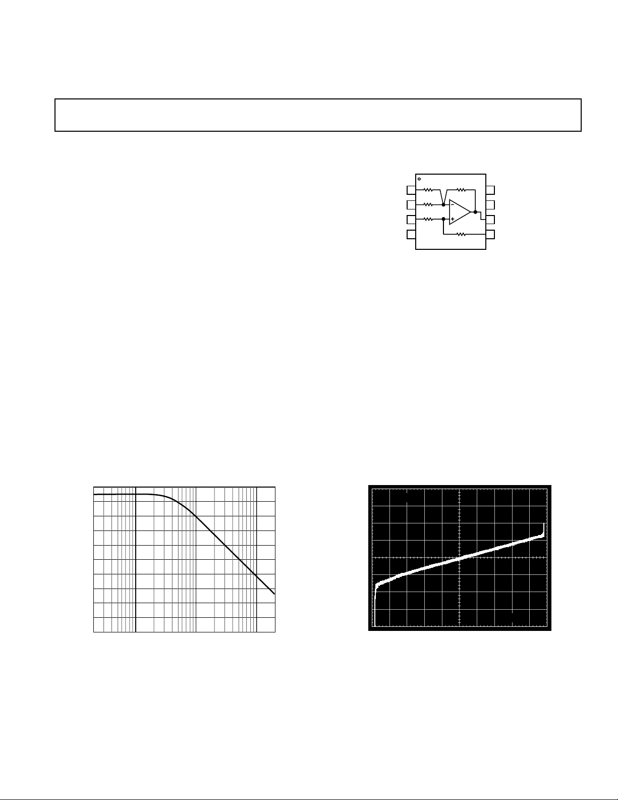
FUNCTIONAL BLOCK DIAGRAM

8-Lead Plastic Mini-DIP (N) and SOIC (R) Packages

REF(–)

–V

–IN

+IN

380k⍀

2

380k⍀

3

4

S

21.1k⍀

1

GENERAL DESCRIPTION

The AD629 is a difference amplifier with a very high input
common-mode voltage range. It is a precision device that
allows the user to accurately measure differential signals in the
presence of high common-mode voltages up to ±270 V.

The AD629 can replace costly isolation amplifiers in applications
that do not require galvanic isolation. The device will operate
over a ±270 V common-mode voltage range and has inputs
that are protected from common-mode or differential mode
transients up to ±500 V.

The AD629 has low offset, low offset drift, low gain error drift,
as well as low common-mode rejection drift, and excellent CMRR
over a wide frequency range.

The AD629 is available in low-cost, plastic 8-lead DIP and
SOIC packages. For all packages and grades, performance is
guaranteed over the entire industrial temperature range from
–40°C to +85°C.

380k⍀

20k⍀

AD629

NC = NO CONNECT

NC

8

7

+V

6

OUTPUT

5

REF(+)

S

100

95

90

85

80

75

70

65

60

COMMON-MODE REJECTION RATIO – dB

55

50

20 100

FREQUENCY – Hz

1k 10k 20k

Figure 1. Common-Mode Rejection Ratio vs. Frequency

REV. A

Information furnished by Analog Devices is believed to be accurate and
reliable. However, no responsibility is assumed by Analog Devices for its
use, nor for any infringements of patents or other rights of third parties
which may result from its use. No license is granted by implication or
otherwise under any patent or patent rights of Analog Devices.

2mV/DIV

OUTPUT ERROR – 2mV/DIV

60V/DIV

–240 –120

COMMON-MODE VOLTAGE – Volts

0 120 240

Figure 2. Common-Mode Operating Range. Error Voltage
vs. Input Common-Mode Voltage

One Technology Way, P.O. Box 9106, Norwood, MA 02062-9106, U.S.A.
Tel: [phone] World Wide Web Site: http://www.analog.com
Fax: [phone] © Analog Devices, Inc., 2000

AD629–SPECIFICATIONS

(TA = 25ⴗC, VS = ⴞ15 V unless otherwise noted)

AD629A AD629B

Parameter Condition Min Typ Max Min Typ Max Unit

GAIN V

Nominal Gain 11V/V
Gain Error 0.01 0.05 0.01 0.03 %
Gain Nonlinearity 4 10 4 10 ppm

Gain vs. Temperature TA = T

OFFSET VOLTAGE

Offset Voltage 0.2 1 0.1 0.5 mV

vs. Temperature T
vs. Supply (PSRR) VS = ±5 V to ±15 V 84 100 90 110 dB

INPUT

Common-Mode Rejection Ratio V

Operating Voltage Range Common-Mode ±270 ±270 V

Input Operating Impedance Common-Mode 200 200 kΩ

OUTPUT

Operating Voltage Range R

Output Short Circuit Current ±25 ±25 mA
Capacitive Load Stable Operation 1000 1000 pF

DYNAMIC RESPONSE

Small Signal –3 dB Bandwidth 500 500 kHz
Slew Rate 1.7 2.1 1.7 2.1 V/µs
Full Power Bandwidth V
Settling Time 0.01%, V

OUTPUT NOISE VOLTAGE

0.01 Hz to 10 Hz 15 15 µV p-p
Spectral Density, ≥100 Hz

1

POWER SUPPLY

Operating Voltage Range ±2.5 ± 18 ± 2.5 ±18 V
Quiescent Current V

TEMPERATURE RANGE

For Specified Performance TA = T

NOTES

1

See Figure 19.

Specifications subject to change without notice.

= ±10 V, RL = 2 kΩ

OUT

= 10 kΩ 1 1 3 ppm

R

L

V

S

A

CM

T

A

V

CM

V

CM

MIN

to T

MAX

3 10 3 10 ppm/°C

= ±5 V 1mV
= T

MIN

to T

MAX

620 310µV/°C

= ±250 V dc 77 88 86 96 dB

= T

MIN

to T

MAX

73 82 dB
= 500 V p-p DC to 500 Hz 77 86 dB
= 500 V p-p DC to 1 kHz 88 90 dB

Differential ±13 ± 13 V

Differential 800 800 kΩ

= 10 kΩ±13 ±13 V

L

= 2 kΩ±12.5 ± 12.5 V

R

L

= ±12 V, RL = 2 kΩ±10 ±10 V

V

S

= 20 V p-p 28 28 kHz

OUT

0.1%, V

0.01%, VCM = 10 V Step, V

= 10 V Step 15 15 µs

OUT

= 10 V Step 12 12 µs

OUT

= 0 V 5 5 µs

DIFF

550 550 nV/√Hz

= 0 V 0.9 1 0.9 1 mA

OUT

T

MIN

to T

MIN

MAX

to T

MAX

1.2 1.2 mA

–40 +85 –40 +85 °C

–2–

REV. A

AD629

WARNING!

ESD SENSITIVE DEVICE

ABSOLUTE MAXIMUM RATINGS

Supply Voltage VS . . . . . . . . . . . . . . . . . . . . . . . . . . . . . ±18 V

Internal Power Dissipation

2

1

DIP (N) . . . . . . . . . . . . . . . . . . . . . . . . See Derating Curves

SOIC (R) . . . . . . . . . . . . . . . . . . . . . . . See Derating Curves

Input Voltage Range, Continuous . . . . . . . . . . . . . . . . ±300 V

Common-Mode and Differential, 10 sec . . . . . . . . . . . ±500 V

Output Short Circuit Duration . . . . . . . . . . . . . . . . Indefinite

Pin 1, Pin 5 . . . . . . . . . . . . . . . . . . –V

– 0.3 V to +VS + 0.3 V

S

Maximum Junction Temperature . . . . . . . . . . . . . . . . . 150°C

Operating Temperature Range . . . . . . . . . . –55°C to +125°C

Storage Temperature Range . . . . . . . . . . . . –65°C to +150°C

Lead Temperature Range (Soldering 60 sec) . . . . . . . . . 300°C

NOTES

1

Stresses above those listed under Absolute Maximum Ratings may cause perma-

nent damage to the device. This is a stress rating only; functional operation of the
device at these or any other conditions above those indicated in the operational
section of this specification is not implied. Exposure to absolute maximum rating
conditions for extended periods may effect device reliability.

2

Specification is for device in free air: 8-Lead Plastic DIP, θJA = 100°C/W; 8-Lead

SOIC Package, θJA = 155°C/W.

2.0

TJ = 150ⴗC

8-LEAD MINI-DIP PACKAGE

1.5

1.0

8-LEAD SOIC PACKAGE

0.5

MAXIMUM POWER DISSIPATION – Watts

0

–40 –30 –20 –100 102030405060708090

–50

AMBIENT TEMPERATURE – ⴗC

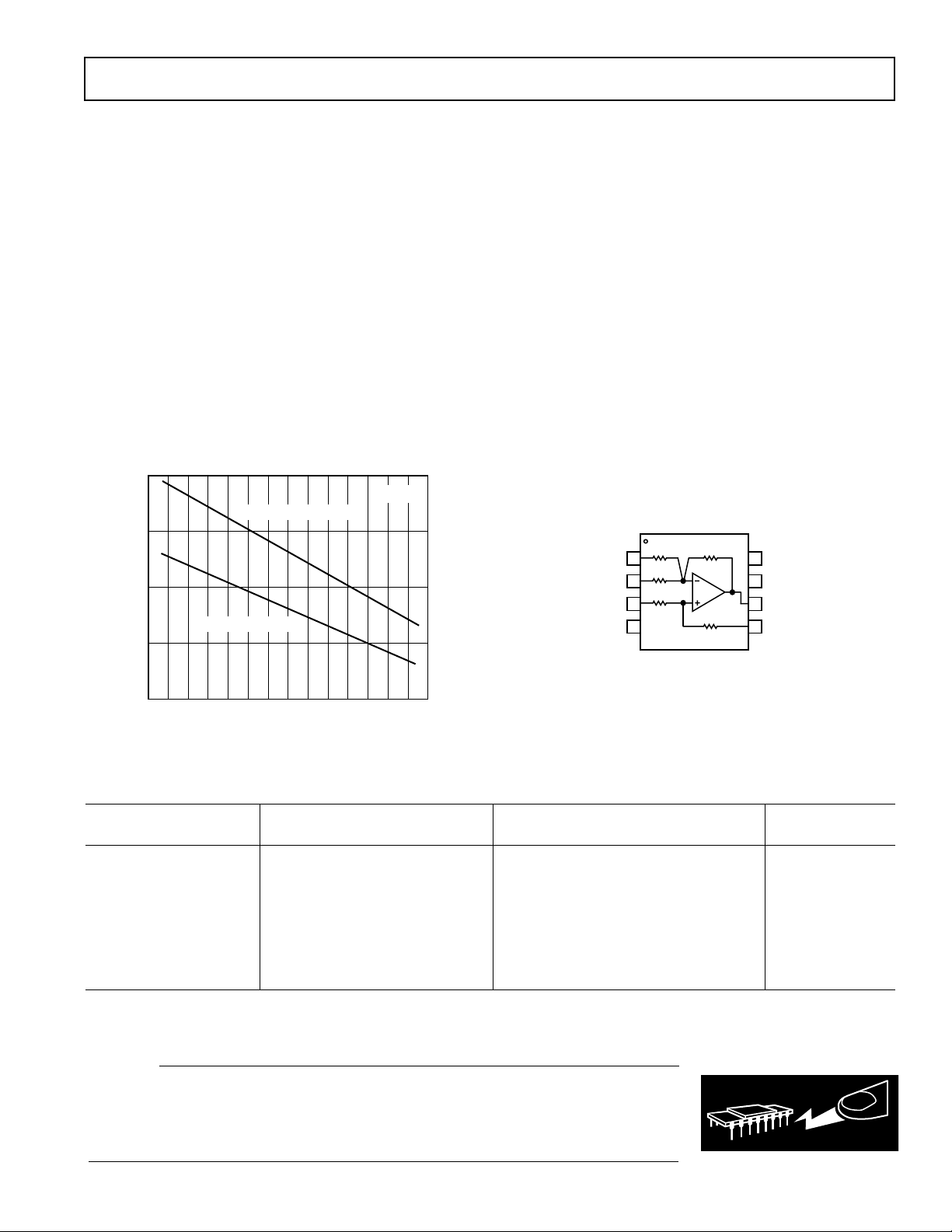
Figure 3. Derating Curve of Maximum Power Dissipation
vs. Temperature for SOIC and PDIP Packages

ORDERING GUIDE

THEORY OF OPERATION

The AD629 is a unity gain differential-to-single-ended amplifier
(Diff Amp) that can reject extremely high common-mode
signals (in excess of 270 V with 15 V supplies). It consists of an
operational amplifier (Op Amp) and a resistor network.

In order to achieve high common-mode voltage range, an internal
resistor divider (Pin 3, Pin 5) attenuates the noninverting signal
by a factor of 20. Other internal resistors (Pin 1, Pin 2, and the
feedback resistor) restores the gain to provide a differential gain
of unity. The complete transfer function equals:

V

= V (+IN ) – V (–IN )

OUT

Laser wafer trimming provides resistor matching so that common­mode signals are rejected while differential input signals are
amplified.

The op amp itself, in order to reduce output drift, uses super
beta transistors in its input stage The input offset current and
its associated temperature coefficient contribute no appreciable
output voltage offset or drift. This has the added benefit of
reducing voltage noise because the corner where 1/f noise becomes
dominant is below 5 Hz. In order to reduce the dependence of
gain accuracy on the op amp, the open-loop voltage gain of the
op amp exceeds 20 million, and the PSRR exceeds 140 dB.

REF(–)

–IN

+IN

–V

21.1k⍀

1

380k⍀

2

380k⍀

3

4

S

380k⍀

20k⍀

AD629

NC = NO CONNECT

NC

8

7

+V

6

OUTPUT

5

REF(+)

S

Figure 4. Functional Block Diagram

Temperature Package Package

Model Range Description Option

AD629AR –40°C to +85°C 8-Lead Plastic SOIC SO-8
AD629AR-REEL
AD629AR-REEL7
AD629BR –40°C to +85°C 8-Lead Plastic SOIC SO-8
AD629BR-REEL
AD629BR-REEL7

1

2

1

2

–40°C to +85°C 8-Lead Plastic SOIC SO-8
–40°C to +85°C 8-Lead Plastic SOIC SO-8

–40°C to +85°C 8-Lead Plastic SOIC SO-8

–40°C to +85°C 8-Lead Plastic SOIC SO-8
AD629AN –40°C to +85°C 8-Lead Plastic DIP N-8
AD629BN –40°C to +85°C 8-Lead Plastic DIP N-8

NOTES

1

13" Tape and Reel of 2500 each

2

7" Tape and Reel of 1000 each

CAUTION

ESD (electrostatic discharge) sensitive device. Electrostatic charges as high as 4000 V readily
accumulate on the human body and test equipment and can discharge without detection.
Although the AD629 features proprietary ESD protection circuitry, permanent damage may
occur on devices subjected to high energy electrostatic discharges. Therefore, proper ESD
precautions are recommended to avoid performance degradation or loss of functionality.

REV. A

–3–

AD629

–Typical Performance Characteristics

(@25ⴗC, VS = ⴞ15 V unless otherwise noted)

100

90

80

70

60

50

40

30

20

COMMON-MODE REJECTION RATIO – dB

10

0

100

1k 10k 100k

FREQUENCY – Hz

1M 10M

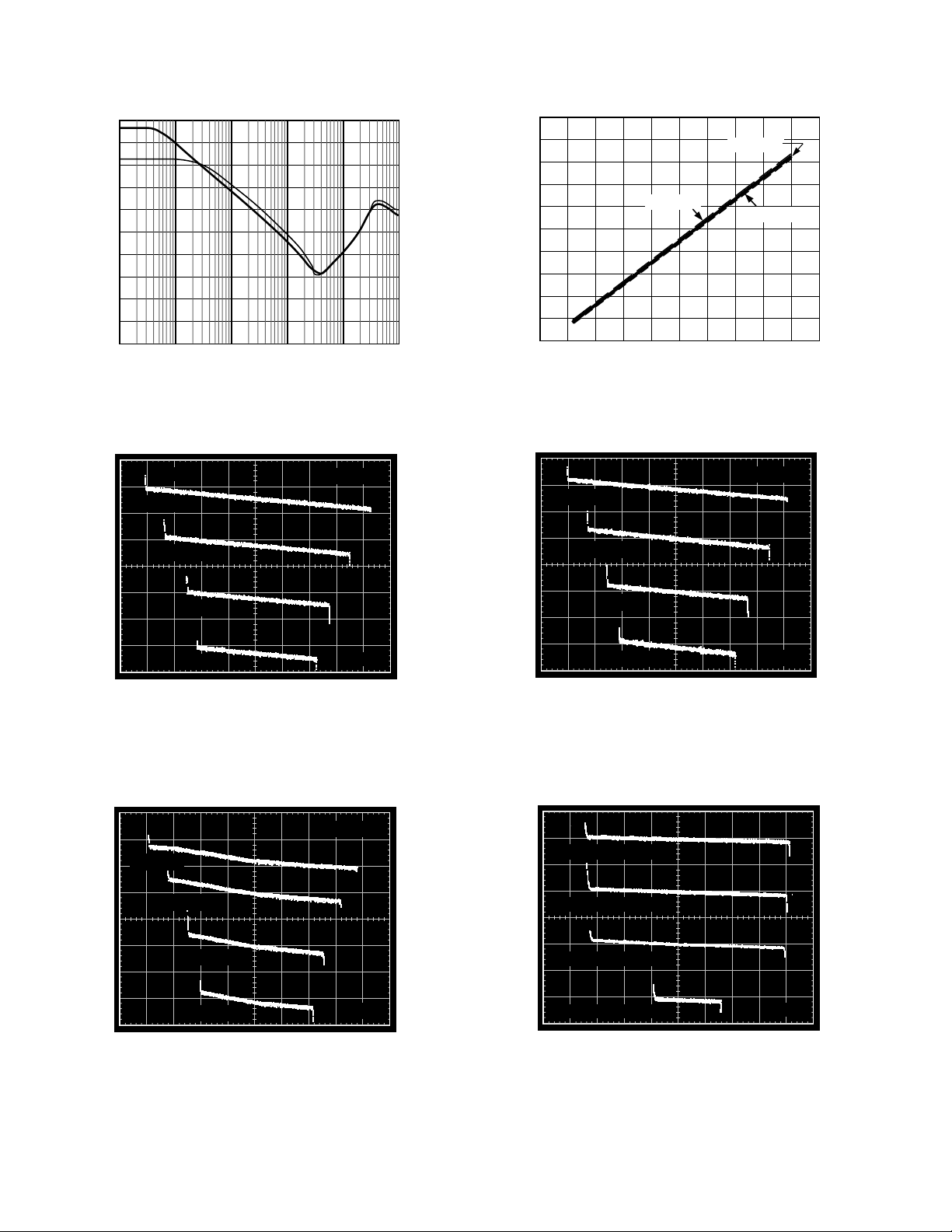
Figure 5. Common-Mode Rejection Ratio vs. Frequency

2mV/DIV

VS = ⴞ18V

VS = ⴞ15V

RL = 10k⍀

400

360

320

280

240

200

160

120

80

COMMON-MODE VOLTAGE – ⴞVolts

40

0

020

POWER SUPPLY VOLTAGE – ⴞVolts

TA = +85ⴗC

TA = +25ⴗC

TA = –40ⴗC

18161412108642

Figure 8. Common-Mode Operating Range vs. Power
Supply Voltage

RL = 2k⍀

VS = ⴞ18V

VS = ⴞ15V

VS = ⴞ12V

OUTPUT ERROR – 2mV/DIV

VS = ⴞ10V

–20 –40 4 20

–8–12–16 8 12 16

V

– Volts

OUT

Figure 6. Typical Gain Error Normalized @ V

4V/DIV

= 0 V and

OUT

Output Voltage Operating Range vs. Supply Voltage,
RL = 10 kΩ (Curves Offset for Clarity)

RL = 1k⍀

VS = ⴞ18V

VS = ⴞ15V

VS = ⴞ12V

OUTPUT ERROR – 2mV/DIV

VS = ⴞ10V

–20 –40 4 20

–8–12–16 8 12 16

V

– Volts

OUT

Figure 7. Typical Gain Error Normalized @ V

4V/DIV

OUT

= 0 V

and Output Voltage Operating Range vs. Supply Voltage,

= 1 kΩ (Curves Offset for Clarity)

R

L

VS = ⴞ12V

OUTPUT ERROR – 2mV/DIV

VS = ⴞ10V

–20 –40 4 20

–8–12–16 8 12 16

V

– Volts

OUT

Figure 9. Typical Gain Error Normalized @ V

4V/DIV

= 0 V and

OUT

Output Voltage Operating Range vs. Supply Voltage,

= 2 kΩ (Curves Offset for Clarity)

R

L

VS = ⴞ5V, RL = 10k⍀

VS = ⴞ5V, RL = 2k⍀

= ⴞ5V, RL = 1k⍀

V

S

OUTPUT ERROR – 2mV/DIV

V

= ⴞ2.5V, RL = 1k⍀

S

–5 –10 1 5

–2–3–4234

– Volts

V

OUT

Figure 10. Typical Gain Error Normalized @ V

1V/DIV

OUT

= 0 V
and Output Voltage Operating Range vs. Supply Voltage
(Curves Offset for Clarity)

–4–

REV. A

AD629

OUTPUT CURRENT – mA

OUTPUT VOLTAGE – Volts

020

14.0

18161412108642

13.0

12.0

11.0

10.0

9.0

–12.0

–12.5

–13.0

–13.5

–11.5

–40ⴗC

–40ⴗC

+85ⴗC

+25ⴗC

VS = ⴞ15V

–40ⴗC

+85ⴗC

+25ⴗC

ERROR – 0.8ppm/DIV

–10 –5

0510

V

– Volts

OUT

Figure 11. Gain Nonlinearity; VS = ±15 V, RL =10 k

ERROR – 1ppm/DIV

–10 –20 2 10

–4–6–8 468

V

– Volts

OUT

Figure 12. Gain Nonlinearity; VS = ±12 V, RL =10 k

ERROR – 2ppm/DIV

–10 –20 2 10

Ω

Ω

Figure 14. Gain Nonlinearity; VS = ±15 V, RL = 2 k

Figure 15. Output Voltage Operating Range vs. Output
Current; V

= ±15 V

S

–4–6–8 468

V

– Volts

OUT

Ω

ERROR – 6.67ppm/DIV

REV. A

–3.0 –0.6 0 0.6 3.0

Figure 13. Gain Nonlinearity; VS = ±5 V, RL =1 k

–1.2–1.8–2.4 1.2 1.8 2.4

V

– Volts

OUT

Ω

Figure 16. Output Voltage Operating Range vs. Output
Current; V

–5–

11.5

10.5
–40ⴗC

9.5

8.5

7.5

6.5

–9.0

–9.5

OUTPUT VOLTAGE – Volts

–10.0

–10.5

–11.0

020

= ±12 V

S

+85ⴗC

VS = ⴞ12V

–40ⴗC

OUTPUT CURRENT – mA

–40ⴗC

+25ⴗC

+85ⴗC

+25ⴗC

+85ⴗC

18161412108642

AD629

+85ⴗC

–40ⴗC

+85ⴗC

VS = ⴞ5V

+85ⴗC

–40ⴗC

+25ⴗC

020

+85ⴗC

OUTPUT CURRENT – mA

–40ⴗC

+25ⴗC

+25ⴗC

18161412108642

–2.0

–2.5

OUTPUT VOLTAGE – Volts

–3.0

–3.5

–4.0

4.5

3.5

2.5

1.5

0.5

Figure 17. Output Voltage Operating Range vs. Output

120

110

100

= ±5 V

S

+V

S

–V

S

90

80

70

60

50

40

30

Current; V

POWER SUPPLY REJECTION RATIO – dB

RL = 2k⍀

= 0pF

C

L

25mV/DIV

4␮s/DIV

Figure 20. Small Signal Pulse Response; G = 1, RL = 2 k

RL = 2k⍀

= 1000pF

C

L

25mV/DIV

4␮s/DIV

Ω

0.1 1
FREQUENCY – Hz

100 1k10 10k

Figure 18. Power Supply Rejection Ratio vs. Frequency

5.0

4.5

4.0

3.5

3.0

2.5

␮V/ Hz

2.0

1.5

1.0

0.5

0.1 1

0.01
FREQUENCY – Hz

100 1k10 10k 100k

Figure 19. Voltage Noise Spectral Density vs. Frequency

Figure 21. Small Signal Pulse Response; G = 1, RL = 2 kΩ,

= 1000 pF

C

L

G = +1

= 2k⍀

R

L

= 1000pF

C

L

5V/DIV

5␮s/DIV

Figure 22. Large Signal Pulse Response; G = 1,

= 2 kΩ, CL = 1000 pF

R

L

–6–

REV. A

AD629

+1 GAIN ERROR – ppm

350

0

–600

NUMBER OF UNITS

–400 –200 0

50

200

600

400

300

250

200

150

100

N = 2180
n ⬇ 200 PCS. FROM
10 ASSEMBLY LOTS

400

5V/DIV

+10V

V

OUT

0V

OUTPUT
ERROR

1mV/DIV

1mV = 0.01%

10␮s/DIV

Figure 23. Settling Time to 0.01%, For 0 V to 10 V Output

= 2 k

Step; G = –1, R

350

N = 2180
n ⬇ 200 PCS. FROM

300

10 ASSEMBLY LOTS

250

200

150

NUMBER OF UNITS

100

50

Ω

L

5V/DIV

0V

V

OUT

–10V

OUTPUT
ERROR

1mV/DIV

1mV = 0.01%

10␮s/DIV

Figure 26. Settling Time to 0.01% for 0 V to –10 V Output
Step; G = –1, R

300

250

200

150

100

NUMBER OF UNITS

50

= 2 k

Ω

L

N = 2180

⬇

200 PCS. FROM

n
10 ASSEMBLY LOTS

0

–150

–100 –50 0

COMMON-MODE REJECTION RATIO – ppm

50

100

150

Figure 24. Typical Distribution of Common-Mode
Rejection; Package Option N-8

400

N = 2180

350

n ⬇ 200 PCS. FROM
10 ASSEMBLY LOTS

300

250

200

150

NUMBER OF UNITS

100

50

0

–600

–400 –200 0

–1 GAIN ERROR – ppm

200

400

600

Figure 25. Typical Distribution of –1 Gain Error;
Package Option N-8

0

–900

–600 –300 0

OFFSET VOLTAGE – ␮V

300

600

900

Figure 27. Typical Distribution of Offset Voltage;
Package Option N-8

Figure 28. Typical Distribution of +1 Gain Error;
Package Option N-8

REV. A

–7–

AD629

APPLICATIONS
Basic Connections

Figure 29 shows the basic connections for operating the AD629
with a dual supply. A supply voltage of between ±3 V and
±18 V is applied between Pins 7 and 4. Both supplies should be
decoupled close to the pins using 0.1 µF capacitors. 10 µF elec-
trolytic capacitors, also located close to the supply pins, may
also be required if low frequency noise is present on the power
supply. While multiple amplifiers can be decoupled by a single
set of 10 µF capacitors, each in amp should have its own set of

0.1 µF capacitors so that the decoupling point can be located
physically close to the power pins.

+V

S

8

7

6

5

NC

+V

REF(+)

3V TO 18V

0.1␮F

S

V

OUT

= I

(SEE
TEXT)

SHUNT

ⴛ R

SHUNT

I

SHUNT

TEXT)

(SEE

R

SHUNT

REF(–)

–IN

+IN

–V

S

0.1␮F

–V

S

–3V TO –18V

AD629

21.1k⍀

1

380k⍀

2

3

4

380k⍀

380k⍀

20k⍀

NC = NO CONNECT

Figure 29. Basic Connections

The differential input signal, which will typically result from a
load current flowing through a small shunt resistor, is applied to
Pins 2 and 3 with the polarity shown in order to obtain a posi­tive gain. The common-mode range on the differential input
signal can range from –270 V to +270 V and the maximum dif­ferential range is ±13 V. When configured as shown, the device
operates as a simple gain-of-one differential-to-single-ended
amplifier, the output voltage being the shunt resistance times the
shunt current. The output is measured with respect to Pins 1 and 5.

Pins 1 and 5 (REF(–) and REF(+)) should be grounded for a
gain of unity and should be connected to the same low imped­ance ground plane. Failure to do this will result in degraded
common-mode rejection. Pin 8 is a no connect pin and should
be left open.

Single Supply Operation

Figure 30 shows the connections for operating the AD629 with
a single supply. Because the output can swing to within only
about 2 V of either rail, it is necessary to apply an offset to the
output. This can be conveniently done by connecting REF(+) and
REF(–) to a low impedance reference voltage (some analog­to-digital converters provide this voltage as an output), which is
capable of sinking current. Thus, for a single supply of 10 V,

might be set to 5 V for a bipolar input signal. This would

V

REF

allow the output to swing ±3 V around the central 5 V reference
voltage. Alternatively, for unipolar input signals, V

could be

REF

set to about 2 V, allowing the output to swing from +2 V (for a 0 V
input) to within 2 V of the positive rail.

+V

NC

+V

S

REF(+)

S

0.1␮F

OUTPUT = V

OUT

–V

REF

I

SHUNT

R

SHUNT

AD629

REF(–)

V

REF

21.1k⍀

1

380k⍀

–IN

2

380k⍀

+IN

3

–V

S

4

NC = NO CONNECT

8

380k⍀

7

V

X

20k⍀

6

5

V

Y

Figure 30. Operation with a Single Supply

Applying a reference voltage to REF(+) and REF(–) and operating
on a single supply will reduce the input common-mode range of
the AD629. The new input common-mode range depends upon
the voltage at the inverting and noninverting inputs of the internal
operational amplifier, labeled V

and VY in Figure 30. These

X

nodes can swing to within 1 V of either rail. So for a (single)
supply voltage of 10 V, V
9 V. If V

is set to 5 V, the permissible common-mode range

REF

and VY can range between 1 V and

X

is +85 V to –75 V. The common-mode voltage ranges can be
calculated using the following equation.

VVV

±

=±

(

)

CM X Y REF

−20 19

(

)

/

System-Level Decoupling and Grounding

The use of ground planes is recommended to minimize the
impedance of ground returns (and hence the size of dc errors).
Figure 31 shows how to work with grounding in a mixed-signal
environment, that is, with digital and analog signals present. In
order to isolate low-level analog signals from a noisy digital
environment, many data-acquisition components have separate
analog and digital ground returns. All ground pins from mixed­signal components such as analog-to-digital converters should
be returned through the “high quality” analog ground plane.
This includes the digital ground lines of mixed-signal converters
that should also be connected to the analog ground plane. This
may seem to break the rule of keeping analog and digital grounds
separate, but in general, there is also a requirement to keep the
voltage difference between digital and analog grounds on a con­verter as small as possible (typically <0.3 V). The increased
noise, caused by the converter’s digital return currents flowing
through the analog ground plane, will typically be negligible.
Maximum isolation between analog and digital is achieved by
connecting the ground planes back at the supplies. Note that
Figure 31, as drawn, suggests a “star” ground system for the
analog circuitry, with all ground lines being connected, in this
case, to the ADC’s analog ground. However, when ground planes
are used, it is sufficient to connect ground pins to the nearest
point on the low impedance ground plane.

–8–

REV. A

AD629

V

OUT

REF(–)

–IN

+IN

–V

S

NC

+V

S

REF(+)

AD629

380k⍀

380k⍀

380k⍀

20k⍀

NC = NO CONNECT

0.1␮F

+V

S

R

SHUNT

8

7

6

5

1

2

3

4

R

COMP

–V

S

0.1␮F

I

SHUNT

21.1k⍀

DIGITAL

POWER SUPPLY

GND

GND

12

␮PROCESSOR

0.1␮F

+5V

V

DD

+IN

–IN

0.1␮F 0.1␮F

–V

S

AD629

REF(–)

ANALOG POWER

+V

S

V

OUT

REF(+)

SUPPLY

+5V GND–5V

0.1␮F

V

DD

V

IN1

V

IN2

AGND

AD7892-2

DGND

Figure 31. Optimal Grounding Practice for a Bipolar Supply
Environment with Separate Analog and Digital Supplies

+IN

–IN

+V

AD629

REF(–)

0.1␮F

S

–V

S

V

OUT

REF(+)

POWER SUPPLY

+5V

V

V

V

DD

IN

REF

GND

0.1␮F

AGND DGND

ADC

0.1␮F

VDDGND

␮PROCESSOR

shows some sample error voltages generated by a common-mode
voltage of 200 V dc with shunt resistors from 20 Ω to 2000 Ω.
Assuming that the shunt resistor has been selected to utilize the
full ±10 V output swing of the AD629, the error voltage becomes
quite significant as R

Table I. Error Resulting from Large Values of R

SHUNT

increases.

SHUNT

(Uncompensated Circuit)

RS (⍀) Error V

(V) Error Indicated (mA)

OUT

20 0.01 0.5
1000 0.498 0.498
2000 1 0.5

If it is desired to measure low current or current near zero in a
high common-mode environment, an external resistor equal to
the shunt resistor value may be added to the low impedance side
of the shunt resistor as shown in Figure 33.

Figure 32. Optimal Ground Practice in a Single Supply
Environment

If there is only a single power supply available, it must be shared
by both digital and analog circuitry. Figure 32 shows how to
minimize interference between the digital and analog circuitry.
In this example, the ADC’s reference is used to drive the
AD629’s REF(+) and REF(–) pins. This means that the reference
must be capable of sourcing and sinking a current equal to V

CM

/

200 kΩ. As in the previous case, separate analog and digital

Figure 33. Compensating for Large Sense Resistors

Output Filtering

A simple 2-pole low-pass Butterworth filter can be implemented
using the OP177 at the output of the AD629 to limit noise at
the output, as shown in Figure 34. Table II gives recommended
component values for various corner frequencies, along with the
peak-to-peak output noise for each case.

ground planes should be used (reasonably thick traces can be
used as an alternative to a digital ground plane). These ground
planes should be connected at the power supply’s ground pin.
Separate traces (or power planes) should be run from the power
supply to the supply pins of the digital and analog circuits. Ideally,
each device should have its own power supply trace, but these
can be shared by a number of devices as long as a single trace is
not used to route current to both digital and analog circuitry.

Using a Large Sense Resistor

Insertion of a large shunt resistance across the input Pins 2 and 3
will imbalance the input resistor network, introducing a common­mode error. The magnitude of the error will depend on the
common-mode voltage and the magnitude of R

SHUNT

. Table I

AD629

21.1k⍀

1

380k⍀

2

380k⍀

3

–V

S

4

NC = NO CONNECT

380k⍀

20k⍀

–IN

+IN

–V

0.1␮F

REF(–)

S

Figure 34. Filtering of Output Noise Using a 2-Pole
Butterworth Filter

8

7

6

5

+V

NC

+V

S

REF(+)

S

0.1␮F

+V

S

OP177

–V

0.1␮F

0.1␮F

S

C1

R2

R1

C2

Table II. Recommended Values for 2-Pole Butterworth Filter

Corner Frequency R1 R2 C1 C2 Output Noise (p-p)

No Filter 3.2 mV
50 kHz 2.94 kΩ ± 1% 1.58 kΩ ± 1% 2.2 nF ± 10% 1 nF ± 10% 1 mV
5 kHz 2.94 kΩ ± 1% 1.58 kΩ ± 1% 22 nF ± 10% 10 nF ± 10% 0.32 mV
500 Hz 2.94 kΩ ± 1% 1.58 kΩ ± 1% 220 nF ± 10% 0.1 µF ± 10% 100 µV
50 Hz 2.7 kΩ ± 10% 1.5 kΩ ± 10% 2.2 µF ± 20% 1 µF ± 20% 32 µV

REV. A

–9–

V

OUT

AD629

Output Current and Buffering

The AD629 is designed to drive loads of 2 kΩ to within 2 V of
the rails, but can deliver higher output currents at lower output
voltages (see Figure 15). If higher output current is required,
the AD629’s output should be buffered with a precision op
amp such as the OP113 as shown in Figure 35. This op amp
can swing to within 1 V of either rail while driving a load as
small as 600 Ω.

+V

S

OP113

–V

S

0.1␮F

0.1␮F

V

OUT

–IN

+IN

–V

0.1␮F

REF(–)

S

AD629

21.1k⍀

1

380k⍀

2

3

4

380k⍀

380k⍀

20k⍀

NC = NO CONNECT

8

7

6

5

NC

0.1␮F

REF(+)

Figure 35. Output Buffering Application

A Gain of 19 Differential Amplifier

While low level signals can be connected directly to the –IN and
+IN inputs of the AD629, differential input signals can also be
connected as shown in Figure 36 to give a precise gain of 19.
However, large common-mode voltages are no longer permissible.
Cold junction compensation can be implemented using a tempera­ture sensor such as the AD590.

+V

8

7

6

5

NC

0.1␮F

REF(+)

S

V

OUT

THERMOCOUPLE

REF(–)

1

–IN

2

+IN

3

V

REF

4

AD629

21.1k⍀

380k⍀

380k⍀

380k⍀

20k⍀

NC = NO CONNECT

Figure 36. A Gain of 19 Thermocouple Amplifier

Error Budget Analysis Example 1

In the dc application below, the 10 A output current from a
device with a high common-mode voltage (such as a power sup­ply or current-mode amplifier) is sensed across a 1 Ω shunt
resistor (Figure 37). The common-mode voltage is 200 V, and
the resistor terminals are connected through a long pair of lead
wires located in a high-noise environment, for example, 50 Hz/
60 Hz 440 V ac power lines. The calculations in Table III
assume an induced noise level of 1 V at 60 Hz on the leads, in
addition to a full-scale dc differential voltage of 10 V. The error
budget table quantifies the contribution of each error source.
Note that the dominant error source in this example is due to
the dc common-mode voltage.

Table III. AD629 vs. INA117 Error Budget Analysis Example 1 (VCM = 200 V dc)

Error, ppm of FS

Error Source AD629 INA117 AD629 INA117

ACCURACY, T

Initial Gain Error (0.0005 × 10) ÷ 10 V × 10
Offset Voltage (0.001 V ÷ 10 V) × 10

= 25°C

A

6

6

(0.0005 × 10) ÷ 10 V × 10
(0.002 V ÷ 10 V) × 10

6

6

500 500
100 200

DC CMR (Over Temperature) (224 × 10-6 × 200 V) ÷ 10 V × 106(500 × 10-6 × 200 V) ÷ 10 V × 1064,480 10,000

Total Accuracy Error: 5,080 10,700

TEMPERATURE DRIFT (85°C)

Gain 10 ppm/°C × 60°C 10 ppm/°C × 60°C 600 600
Offset Voltage (20 µV/°C × 60°C) × 106/10 V (40 µV/°C × 60°C) × 106/10 V 120 240

Total Drift Error: 720 840

RESOLUTION

Noise, Typ, 0.01–10 Hz, µV p-p 15 µV ÷ 10 V × 10
CMR, 60 Hz (141 × 10

–6

Nonlinearity (10–5 × 10 V) ÷ 10 V × 10

6

× 1 V) ÷ 10 V × 106(500 × 10–6 × 1 V) ÷ 10 V × 10

6

25 µV ÷ 10 V × 10

(10–5 × 10 V) ÷ 10 V × 10

6

6

6

23
14 50
10 10

Total Resolution Error: 26 63

Total Error: 5,826 11,603

–10–

REV. A

AD629

OUTPUT

CURRENT

1⍀

SHUNT

10 AMPS
200V

DC

CM

TO GROUND

60Hz

POWER LINE

REF(–)

–V

S

21.1k⍀

1

380k⍀

–IN

2

380k⍀

+IN

3

4

AD629

0.1␮F

NC = NO CONNECT

380k⍀

20k⍀

8

7

6

5

NC

0.1␮F

REF(+)

+V

S

V

OUT

Figure 37. Error Budget Analysis Example 1. VIN = 10 V
Full-Scale, V

= 200 V DC. R

CM

= 1 Ω, 1 V p-p 60 Hz

SHUNT

Power-Line Interference

Error Budget Analysis Example 2

This application is similar to the previous example except that
the sensed load current is from an amplifier with an ac common­mode component of ±100 V (frequency = 500 Hz) present on
the shunt (Figure 38). All other conditions are the same as

before. Note that the same kind of power line interference can
happen as detailed in Example 1. However, the ac common­mode component of 200 V p-p coming from the shunt is much
larger than the interference of 1 V p-p, so that this interference
component can be neglected.

OUTPUT

CURRENT

1⍀

SHUNT

10 AMPS

AC CM

ⴞ100V
TO GROUND

60Hz

POWER LINE

REF(–)

–V

S

21.1k⍀

1

380k⍀

–IN

2

380k⍀

+IN

3

4

AD629

0.1␮F

NC = NO CONNECT

380k⍀

20k⍀

8

7

6

5

NC

0.1␮F

REF(+)

+V

S

V

OUT

Figure 38. Error Budget Analysis Example 2. VIN = 10 V
Full-Scale, V

= ±100 V at 500 Hz, R

CM

SHUNT

= 1

Ω

Table IV. AD629 vs. INA117 AC Error Budget Example 2 (VCM = ⴞ100 V @ 500 Hz)

Error, ppm of FS

Error Source AD629 INA117 AD629 INA117

ACCURACY, T

Initial Gain Error (0.0005 × 10) ÷ 10 V × 10
Offset Voltage (0.001 V ÷ 10 V) × 10

= 25°C

A

6

6

(0.0005 × 10) ÷ 10 V × 10
(0.002 V ÷ 10 V) × 10

6

6

500 500
100 200

Total Accuracy Error: 600 700

TEMPERATURE DRIFT (85°C)

Gain 10 ppm/°C × 60°C 10 ppm/°C × 60°C 600 600
Offset Voltage (20 µV/°C × 60°C) × 106/10 V (40 µV/°C × 60°C) × 106/10 V 120 240

Total Drift Error: 720 840

RESOLUTION

Noise, Typ, 0.01–10 Hz, µV p-p 15 µV ÷ 10 V × 10
CMR @ 60 Hz (141 × 10
Nonlinearity (10

–6

–5

× 10 V) ÷ 10 V × 10

6

× 1 V) ÷ 10 V × 106(500 × 10–6 × 1 V) ÷ 10 V × 10

6

25 µV ÷ 10 V × 10

(10–5 × 10 V) ÷ 10 V × 10

6

6

6

23
14 50
10 10

AC CMR @ 500 Hz (141 × 10–6 × 200 V) ÷ 10 V × 106(500 × 10–6 × 200 V) ÷ 10 V × 1062,820 10,000

Total Resolution Error: 2,846 10,063

Total Error: 4,166 11,603

REV. A

–11–

AD629

OUTLINE DIMENSIONS

Dimensions shown in inches and (mm).

PIN 1

0.210

(5.33)

MAX

0.160 (4.06)

0.115 (2.93)

0.022 (0.558)

0.014 (0.356)

8-Lead Plastic DIP

(N-8)

0.430 (10.92)

0.348 (8.84)

8

0.100 (2.54)

5

0.280 (7.11)

14

BSC

0.240 (6.10)

0.060 (1.52)

0.015 (0.38)

0.070 (1.77)

0.045 (1.15)

0.130
(3.30)
MIN

SEATING
PLANE

0.325 (8.25)

0.300 (7.62)

0.015 (0.381)

0.008 (0.204)

0.195 (4.95)

0.115 (2.93)

0.1574 (4.00)

0.1497 (3.80)

PIN 1

0.0098 (0.25)

0.0040 (0.10)

SEATING

0.1968 (5.00)

0.1890 (4.80)

85

0.0500 (1.27)

PLANE

8-Lead SOIC

0.2440 (6.20)

0.2284 (5.80)

41

BSC

0.0192 (0.49)

0.0138 (0.35)

(SO-8)

0.0688 (1.75)

0.0532 (1.35)

0.0098 (0.25)

0.0075 (0.19)

0.0196 (0.50)

0.0099 (0.25)

8ⴗ

0.0500 (1.27)

0ⴗ

0.0160 (0.41)

ⴛ 45ⴗ

C3717a–6–3/00 (rev. A)

–12–

PRINTED IN U.S.A.

REV. A