


1-Port VNA Series
R54
R140
R60
R180/RP180
Operating Manual
Software version 18.3.0
July 2018

T A B L E O F C O N T E N T S
INTRODUCTION ....................................................................................................................... 8
SAFETY INSTRUCTIONS .......................................................................................................... 9
1. GENERAL OVERVIEW ....................................................................................................... 11
1.1 Description ........................................................................................................................................ 11
1.2 Specifications ................................................................................................................................... 11
1.3 Measurement Capabilities ........................................................................................................... 11
1.4 Principle of Operation .................................................................................................................. 16
2. PREPARATION FOR USE .................................................................................................. 18
2.1 General Information ...................................................................................................................... 18
2.2 Software Installation ..................................................................................................................... 20
2.3 Top Panel ........................................................................................................................................... 20
2.4 Test Port ............................................................................................................................................. 23
2.5 Mini B USB Port ............................................................................................................................... 23
2.6 External Trigger Signal Input Connector (R140 model only) ........................................ 24
2.7 External Reference Frequency Input Connector (R140 model only) .......................... 24
2.8 Reference Frequency Input/Output Connector (R60 and R180 model
only) 24
2.9 External Trigger Signal Input/Output Connector (R60 and R180 model
only) 25
3. GETTING STARTED .......................................................................................................... 26
3.1 Analyzer Preparation for Reflection Measurement ........................................................... 27
3.2 Analyzer Presetting ........................................................................................................................ 27
3.3 Stimulus Setting .............................................................................................................................. 28
3.4 IF Bandwidth Setting .................................................................................................................... 29
3.5 Number of Traces, Measured Parameter and Display Format Setting ...................... 30
3.6 Trace Scale Setting ........................................................................................................................ 31
3.7 Analyzer Calibration for Reflection Coefficient Measurement ..................................... 31
3.8 SWR and Reflection Coefficient Phase Analysis Using Markers .................................. 34
4. MEASUREMENT CONDITIONS SETTING ......................................................................... 36
4.1 Screen Layout and Functions ..................................................................................................... 36
4.1.1 Left and Right Softkey Menu Bars .................................................................................... 36
4.1.2 Top Menu Bar ........................................................................................................................... 37
4.1.3 Instrument Status Bar ........................................................................................................... 40
4.2 Channel Window Layout and Functions ................................................................................ 42
4.2.1 Channel Title Bar .................................................................................................................... 43
4.2.2 Trace Status Field ................................................................................................................... 43
4.2.3 Graph Area ................................................................................................................................. 46
4.2.4 Markers ........................................................................................................................................ 47
4.2.5 Channel Status Bar ................................................................................................................. 48
4.3 Quick Channel Setting Using Mouse....................................................................................... 49
4.3.1 Active Channel Selection ..................................................................................................... 49
2

4.3.2 Active Trace Selection .......................................................................................................... 50
4.3.3 Display Format Setting ......................................................................................................... 50
4.3.4 Trace Scale Setting................................................................................................................. 50
4.3.5 Reference Level Setting ....................................................................................................... 51
4.3.6 Marker Stimulus Value Setting .......................................................................................... 52
4.3.7 Switching between Start/Center and Stop/Span Modes ......................................... 52
4.3.8 Start/Center Value Setting .................................................................................................. 53
4.3.9 Stop/Span Value Setting ...................................................................................................... 53
4.3.10 Sweep Points Number Setting ........................................................................................ 54
4.3.11 IF Bandwidth Setting .......................................................................................................... 54
4.3.12 Power Level Setting ............................................................................................................ 55
4.4 Channel and Trace Display Setting ......................................................................................... 55
4.4.1 Setting the Number of Channel Windows ..................................................................... 55
4.4.2 Channel Activating ................................................................................................................. 56
4.4.3 Active Channel Window Maximizing ............................................................................... 57
4.4.4 Number of Traces Setting .................................................................................................... 58
4.4.5 Active Trace Selection .......................................................................................................... 59
4.5 Measurement Parameters Setting ............................................................................................ 62
4.5.1 S-Parameters............................................................................................................................. 62
4.5.2 Trace Format ............................................................................................................................. 62
4.5.3 Rectangular Format ............................................................................................................... 63
4.5.4 Polar Format ............................................................................................................................. 65
4.5.5 Smith Chart Format ................................................................................................................ 66
4.5.6 Data Format Setting ............................................................................................................... 68
4.6 Trigger Setting ................................................................................................................................. 69
4.6.1 External Trigger (except R54) ............................................................................................ 71
4.6.1.1 Point Feature ..................................................................................................................... 71
4.6.1.2 External Trigger Polarity .............................................................................................. 71
4.6.1.3 External Trigger Position ............................................................................................. 72
4.6.1.4 External Trigger Delay .................................................................................................. 73
4.6.2 Trigger Output (except R54/R140) .................................................................................. 76
4.6.2.1 Switching ON/OFF Trigger Output ........................................................................... 77
4.6.2.2 Trigger Output Polarity ................................................................................................. 78
4.6.2.3 Trigger Output Function ............................................................................................... 79
4.7 Scale Setting ..................................................................................................................................... 80
4.7.1 Rectangular Scale ................................................................................................................... 80
4.7.2 Rectangular Scale Setting ................................................................................................... 80
4.7.3 Circular Scale ............................................................................................................................ 81
4.7.4 Circular Scale Setting ............................................................................................................ 81
4.7.5 Automatic Scaling ................................................................................................................... 82
4.7.6 Reference Level Automatic Selection ............................................................................. 83
4.7.7 Electrical Delay Setting ........................................................................................................ 83
4.7.8 Phase Offset Setting .............................................................................................................. 84
4.8 Stimulus Setting .............................................................................................................................. 86
4.8.1 Sweep Type Setting ............................................................................................................... 86
4.8.2 Sweep Span Setting ............................................................................................................... 86
3

4.8.3 Sweep Points Setting ............................................................................................................ 87
4.8.4 Stimulus Power Setting ........................................................................................................ 88
4.8.5 Segment Table Editing ......................................................................................................... 88
4.9 Trigger Setting ................................................................................................................................. 91
4.10 Measurement Optimizing ......................................................................................................... 92
4.10.1 IF Bandwidth Setting .......................................................................................................... 92
4.10.2 Averaging Setting ................................................................................................................. 92
4.10.3 Smoothing Setting ............................................................................................................... 93
4.10.4 Trace Hold Function ............................................................................................................ 95
4.11 Cable Specifications .................................................................................................................... 96
4.11.1 Selecting the type of cable ............................................................................................... 96
4.11.2 Manually specify Velocity Factor and Cable Loss .................................................... 97
4.11.3 Editing table of cables........................................................................................................ 98
5. CALIBRATION AND CALIBRATION KIT ......................................................................... 100
5.1 General Information .................................................................................................................... 100
5.1.1 Measurement Errors ............................................................................................................. 100
5.1.2 Systematic Errors .................................................................................................................. 100
5.1.2.1 Directivity Error .............................................................................................................. 101
5.1.2.2 Source Match Error ....................................................................................................... 101
5.1.2.3 Reflection Tracking Error ........................................................................................... 101
5.1.3 Error Modeling ....................................................................................................................... 101
5.1.3.1 One-Port Error Model .................................................................................................. 101
5.1.4 Analyzer Test Port Defining .............................................................................................. 102
5.1.5 Calibration Steps ................................................................................................................... 103
5.1.6 Calibration Methods ............................................................................................................. 104
5.1.6.1 Normalization ................................................................................................................. 104
5.1.6.2 Expanded Normalization ............................................................................................ 105
5.1.6.3 Full One-Port Calibration ........................................................................................... 105
5.1.6.4 Waveguide Calibration ................................................................................................ 106
5.1.7 Calibration Standards and Calibration Kits ................................................................ 107
5.1.7.1 Types of Calibration Standards ................................................................................ 107
5.1.7.2 Calibration Standard Model ...................................................................................... 107
5.2 Calibration Procedures ............................................................................................................... 110
5.2.1 Calibration Kit Selection .................................................................................................... 110
5.2.2 Reflection Normalization ................................................................................................... 112
5.2.3 Full One-Port Calibration ................................................................................................... 114
5.2.4 Error Correction Disabling ................................................................................................. 116
5.2.5 Error Correction Status ....................................................................................................... 116
5.2.6 System Impedance Z0 ......................................................................................................... 117
5.2.7 Port Extension ........................................................................................................................ 117
5.2.8 Auto Port Extension ............................................................................................................. 119
5.3 Calibration Kit Management .................................................................................................... 121
5.3.1 Calibration Kit Selection for Editing ............................................................................. 121
5.3.2 Calibration Kit Label Editing ............................................................................................ 121
5.3.3 Predefined Calibration Kit Restoration ........................................................................ 122
4

5.3.4 Calibration Standard Editing ............................................................................................ 124
5.3.5 Calibration Standard Defining by S-Parameter File ................................................ 126
5.4 Automatic Calibration Module ................................................................................................ 128
5.4.1 Automatic Calibration Module Features ...................................................................... 129
5.4.2 Automatic Calibration Procedure ................................................................................... 130
6. MEASUREMENT DATA ANALYSIS ................................................................................. 131
6.1 Markers ............................................................................................................................................. 131
6.1.1 Marker Adding ........................................................................................................................ 132
6.1.2 Marker Deleting ..................................................................................................................... 133
6.1.3 Marker Stimulus Value Setting ........................................................................................ 133
6.1.4 Marker Activating .................................................................................................................. 134
6.1.5 Reference Marker Feature ................................................................................................. 134
6.1.6 Marker Properties .................................................................................................................. 136
6.1.6.1 Marker Coupling Feature ............................................................................................ 136
6.1.6.2 Marker Value Indication Capacity ........................................................................... 138
6.1.6.3 Multi Marker Data Display ......................................................................................... 138
6.1.6.4 Marker Data Alignment ............................................................................................... 139
6.1.6.5 Memory trace value display ...................................................................................... 140
6.1.7 Marker Position Search Functions .................................................................................. 141
6.1.7.1 Search for Maximum and Minimum ....................................................................... 142
6.1.7.2 Search for Peak............................................................................................................... 143
6.1.7.3 Search for Target Level ............................................................................................... 145
6.1.7.4 Search Tracking .............................................................................................................. 147
6.1.7.5 Search Range .................................................................................................................. 147
6.1.8 Marker Math Functions ....................................................................................................... 148
6.1.8.1 Trace Statistics ............................................................................................................... 149
6.1.8.2 Bandwidth Search ......................................................................................................... 151
6.1.8.3 Flatness ............................................................................................................................. 155
6.1.8.4 RF Filter Statistics ......................................................................................................... 157
6.2 Memory Trace Function ............................................................................................................. 160
6.2.1 Saving Trace into Memory ................................................................................................. 161
6.2.2 Memory Trace Deleting ...................................................................................................... 161
6.2.3 Trace Display Setting .......................................................................................................... 162
6.2.4 Memory Trace Math ............................................................................................................. 163
6.3 Fixture Simulation ........................................................................................................................ 164
6.3.1 Port Z Conversion ................................................................................................................. 164
6.3.2 De-embedding ........................................................................................................................ 165
6.3.3 Embedding ............................................................................................................................... 167
6.4 Time Domain Transformation .................................................................................................. 168
6.4.1 Time Domain Transformation Activating .................................................................... 170
6.4.2 Time Domain Transformation Span ............................................................................... 172
6.4.3 Time Domain Transformation Type ............................................................................... 174
6.4.4 Time Domain Transformation Window Shape Setting ........................................... 174
6.4.5 Frequency Harmonic Grid Setting .................................................................................. 175
6.5 Time Domain Gating ................................................................................................................... 177
5

6.5.1 Time Domain Gate Activating .......................................................................................... 178
6.5.2 Time Domain Gate Span..................................................................................................... 178
6.5.3 Time Domain Gate Type ..................................................................................................... 179
6.5.4 Time Domain Gate Shape Setting .................................................................................. 179
6.6 S-Parameter Conversion ............................................................................................................ 180
6.7 Limit Test ......................................................................................................................................... 182
6.7.1 Limit Line Editing ................................................................................................................. 183
6.7.2 Limit Test Enabling/Disabling ......................................................................................... 185
6.7.3 Limit Test Display Management ..................................................................................... 185
6.7.4 Limit Line Offset .................................................................................................................... 186
6.8 Ripple Limit Test........................................................................................................................... 187
6.8.1 Ripple Limit Editing ............................................................................................................. 187
6.8.2 Ripple Limit Enabling/Disabling ..................................................................................... 189
6.8.3 Ripple Limit Test Display Management ....................................................................... 189
7. CABLE LOSS MEASUREMENT ........................................................................................ 191
7.1 Cable Loss Measurement Algorithm ..................................................................................... 191
8. ANALYZER DATA OUTPUT ............................................................................................ 193
8.1 Analyzer State ................................................................................................................................ 193
8.1.1 Analyzer State Saving ......................................................................................................... 193
8.1.2 Analyzer State Recalling .................................................................................................... 195
8.1.3 Autosave and Autorecall State of Analyzer ................................................................ 195
8.2 Channel State ................................................................................................................................. 196
8.2.1 Channel State Saving .......................................................................................................... 196
8.2.2 Channel State Recalling ..................................................................................................... 197
8.3 Trace Data CSV File ..................................................................................................................... 199
8.3.1 CSV File Saving ...................................................................................................................... 199
8.4 Trace Data Touchstone File ...................................................................................................... 201
8.4.1 Touchstone File Saving ...................................................................................................... 202
8.4.2 Touchstone File Recalling ................................................................................................. 203
8.5 Graph Printing ................................................................................................................................ 205
8.5.1 Graph Printing Procedure .................................................................................................. 205
8.5.2 Quick saving program screen shot ................................................................................. 206
9. SYSTEM SETTINGS ......................................................................................................... 207
9.1 Analyzer Presetting ...................................................................................................................... 207
9.2 Program Exit ................................................................................................................................... 207
9.3 Analyzer System Data ................................................................................................................. 208
9.4 System Correction Setting ........................................................................................................ 208
9.5 User Interface Setting ................................................................................................................. 210
10. SPECIFICS OF WORKING WITH TWO OR MORE DEVICES ........................................ 212
10.1 Installation of additional software...................................................................................... 212
10.2 Connecting devices to a USB port ....................................................................................... 212
10.3 Synchronizing the work of analyzers ................................................................................. 212
10.4 Adding / removing devices ..................................................................................................... 214
6

10.5 Frequency adjustment of the internal generators ........................................................ 214
10.5.1 Manual frequency adjustment ....................................................................................... 215
10.5.2 Automatic frequency adjustment ................................................................................. 215
10.6 Features of analyzers calibration ........................................................................................ 216
10.6.1 Calibration Type .................................................................................................................. 217
10.6.2 Scalar Transmission Normalization............................................................................. 218
10.6.3 Expanded Transmission Normalization ..................................................................... 218
10.7 Selection of the measured S-parameters ......................................................................... 221
11. MAINTENANCE AND STORAGE ................................................................................... 222
11.1 Maintenance Procedures ......................................................................................................... 222
11.2 Instrument Cleaning ................................................................................................................. 222
11.3 Factory Calibration .................................................................................................................... 223
11.4 Storage Instructions .................................................................................................................. 223
Appendix 1 .......................................................................................................................... 224
7

INTRODUCTION
This Operating Manual represents design, specifications, overview of functions,
and detailed operation procedure for the Vector Network Analyzer, to ensure
effective and safe use of the technical capabilities of the instrument by the user.
Vector Network Analyzer operation and maintenance should be performed by
qualified engineers with initial experience in operating of microwave circuits and
PC.
The following abbreviations are used in this Manual:
PC – Personal Computer
DUT – Device Under Test
IF – Intermediate Frequency
CW – Continuous Wave
SWR – Standing Wave Ratio
VNA – Vector Network Analyzer
8

SAFETY INSTRUCTIONS
Carefully read through the following safety instructions before putting the
Analyzer into operation. Observe all the precautions and warnings provided in this
Manual for all the phases of operation, service, and repair of the Analyzer.
The VNA must be used only by skilled and specialized staff or thoroughly trained
personnel with the required skills and knowledge of safety precautions.
The Analyzer complies with INSTALLATION CATEGORY I as well as POLLUTION
DEGREE 2 in IEC61010–1.
The Analyzer is a MEASUREMENT CATEGORY I (CAT I) device. Do not use as CAT II,
III, or IV device.
The Analyzer is tested in stand-alone condition or in combination with the
accessories supplied by Copper Mountain Technologies against the requirement of
the standards described in the Declaration of Conformity. If it is used as a system
component, compliance of related regulations and safety requirements are to be
confirmed by the builder of the system.
Never operate the Analyzer in the environment containing inflammable gasses or
fumes.
Operators must not remove the cover or part of the housing. The Analyzer must
not be repaired by the operator. Component replacement or internal adjustment
must be performed by qualified maintenance personnel only.
Electrostatic discharge can damage your Analyzer when connected or
disconnected from the DUT. Static charge can build up on your body and damage
the sensitive circuits of internal components of both the Analyzer and the DUT. To
avoid damage from electric discharge, observe the following:
Always use a desktop anti static mat under the DUT.
Always wear a grounding wrist strap connected to the desktop anti static
mat via daisy-chained 1 MΩ resistor.
Connect the PC and the body of the DUT to protective grounding before
you start operation.
9

SAFETY INSTRUCTIONS
CAUTION
This sign denotes a hazard. It calls attention to a procedure,
practice or condition that, if not correctly performed or adhered
to, could result in damage to or destruction of part or all of the
instrument.
Note
This sign denotes important information. It calls attention to a
procedure, practice, or condition that is essential for the user to
understand.
10

Measured parameters
S
11,
Cable loss.
Number of
measurement
channels
Up to 4 logical channels. Each logical channel is
represented on the screen as an individual channel
window. A logical channel is defined by such stimulus
signal settings as frequency range, number of test points,
etc.
Data traces
Up to 4 data traces can be displayed in each channel
window. A data trace represents one of such parameters
of the DUT as magnitude and phase of S11, DTF, Cable
loss.
Memory traces
Each of the 4 data traces can be saved into memory for
further comparison with the current values.
Data display formats
SWR, Return loss, Cable loss, Phase, Expanded phase,
Smith chart diagram, DTF SWR, DTF Return loss, Group
delay.
Sweep setup features
Sweep type
Linear frequency sweep, logarithmic frequency sweep,
and segment frequency sweep.
Measured points per
sweep
Set by user from 2 to 100,001.
1. GENERAL OVERVIEW
1.1 Description
The VNA is designed for use in the process of development, adjustment and testing of
antenna-feeder devices in industrial and laboratory facilities, as well as in field,
including operation as a component of an automated measurement system. The
Analyzer is designed for operation with external PC, which is not supplied with it.
1.2 Specifications
The specifications of Analyzer model can be found in its corresponding datasheet.
1.3 Measurement Capabilities
11

GENERAL OVERVIEW
Segment sweep
A frequency sweep within several user-defined
segments. Frequency range, number of sweep points, IF
bandwidth and measurement delay should be set for
each segment.
Power settings
Two modes of output power level.
Power levels depending on device.
Sweep trigger
Trigger modes: continuous, single, hold.
Trace display functions
Trace type
Data trace, memory trace.
Trace math
Data trace modification by math operations: addition,
subtraction, multiplication or division of measured
complex values and memory data.
Auto scaling
Automatic selection of scale division and reference level
value to have the trace most effectively displayed.
Electrical delay
Calibration plane moving to compensate for the delay in
the test setup. Compensation for electrical delay in a
DUT during measurements of deviation from linear
phase.
Phase offset
Phase offset defined in degrees.
Accuracy enhancement
Calibration
Calibration of a test setup (which includes the Analyzer
and adapter) significantly increases the accuracy of
measurements. Calibration allows to correct the errors
caused by imperfections in the measurement system:
system directivity, source match, and tracking.
Calibration methods
The following calibration methods are available:
reflection normalization;
full one-port calibration.
Reflection
normalization
The simplest calibration method.
Full one-port
calibration
Method of calibration that ensures high accuracy.
12

GENERAL OVERVIEW
Factory calibration
The factory calibration of the Analyzer allows performing
measurements without additional calibration and
reduces the measurement error after reflection
normalization.
Mechanical
calibration kits
The user can select one of the predefined calibration kits
of various manufacturers or define own calibration kits.
Electronic calibration
modules
Electronic calibration modules manufactured by COPPER
MOUNTAIN TECHNOLOGIES make the Analyzer
calibration faster and easier than traditional mechanical
calibration.
Defining of calibration
standards
Different methods of calibration standard defining are
available:
standard defining by polynomial model;
standard defining by data (S-parameters).
Error correction
interpolation
When the user changes such settings as start/stop
frequencies and number of sweep points, compared to
the settings of calibration, interpolation or extrapolation
of the calibration coefficients will be applied.
Marker functions
Data markers
Up to 16 markers for each trace. A marker indicates
stimulus value and the measured value in a given point
of the trace.
Reference marker
Enables indication of any maker values as relative to the
reference marker.
Marker search
Search for max, min, peak, or target values on a trace.
Marker search
additional features
User-definable search range. Functions of specific
condition tracking or single operation search.
Setting parameters by
markers
Setting of start, stop and center frequencies by the
stimulus value of the marker and setting of reference
level by the response value of the marker.
Marker math functions
Statistics, bandwidth, flatness, RF filter.
13

GENERAL OVERVIEW
Statistics
Calculation and display of mean, standard deviation and
peak-to-peak in a frequency range limited by two
markers on a trace.
Bandwidth
Determines bandwidth between cutoff frequency points
for an active marker or absolute maximum. The
bandwidth value, center frequency, lower frequency,
higher frequency, Q value, and insertion loss are
displayed.
Flatness
Displays gain, slope, and flatness between two markers
on a trace.
RF filter
Displays insertion loss and peak-to-peak ripple of the
passband, and the maximum signal magnitude in the
stopband. The passband and stopband are defined by
two pairs of markers.
Data analysis
Port impedance
conversion
The function of conversion of the S-parameters
measured at 50 Ω port into the values, which could be
determined if measured at a test port with arbitrary
impedance.
De-embedding
The function allows to exclude mathematically the
effect of the fixture circuit connected between the
calibration plane and the DUT from the measurement
result. This circuit should be described by an Sparameter matrix in a Touchstone file.
Embedding
The function allows to simulate mathematically the DUT
parameters after virtual integration of a fixture circuit
between the calibration plane and the DUT. This circuit
should be described by an S-parameter matrix in a
Touchstone file.
S-parameter
conversion
The function allows conversion of the measured Sparameters to the following parameters: reflection
impedance and admittance, transmission impedance and
admittance, and inverse S-parameters.
14

GENERAL OVERVIEW
Time domain
transformation
The function performs data transformation from
frequency domain into response of the DUT to
radiopulse in time domain. Time domain span is set by
the user arbitrarily from zero to maximum, which is
determined by the frequency step. Windows of various
forms allow better tradeoff between resolution and level
of spurious sidelobes.
Time domain gating
The function mathematically removes unwanted
responses in time domain what allows obtaining
frequency response without influence from the fixture
elements. The function applies reverse transformation
back to frequency domain from the user-defined span in
time domain. Gating filter types are: bandpass or notch.
For better tradeoff between gate resolution and level of
spurious sidelobes the following filter shapes are
available: maximum, wide, normal and minimum.
Other features
Analyzer control
Using external personal computer via USB interface.
Familiar graphical
user interface
Graphical user interface based on Windows operating
system ensures fast and easy Analyzer operation by the
user.
The software interface of Analyzers is compatible with
modern tablet PCs and laptops.
Saving trace data
Saving the traces in graphical format and saving the data
in Touchstone and *.csv (comma separated values)
formats on the hard drive are available.
Remote control
COM/DCOM
Remote control via COM/DCOM. COM automation runs
the user program on an Analyzer PC. DCOM automation
runs the user program on a LAN-networked PC.
Automation of the instrument can be achieved in any
COM/DCOM-compatible language or environment,
including Python, C++, C#, VB.NET, LabVIEW, MATLAB,
Octave, VEE, Visual Basic (Excel) and many others.
Socket
Data transfer between the PC user and the computer
that is connected to the device, can be also performed
via Socket (TCP, port 5025).
15

GENERAL OVERVIEW
1.4 Principle of Operation
The Analyzer consists of the Analyzer Unit, some supplementary accessories, and
personal computer (which is not supplied with the package). The Analyzer Unit is
powered and controlled by PC via USB-interface. The block diagram of the Analyzer is
represented in Figure 1.1.
The Analyzer Unit consists of a source oscillator, a local oscillator, a source power
attenuator, a directional coupler and other components which ensure the Analyzer
operation. The test port is the source of the test signal. The incident and reflected
signals from the directional coupler are supplied into the mixers, where they are
converted into IF, and are transferred further to the 2-channel receiver. The 2-channel
receiver, after filtration, digitally encodes the signals and supplies them for further
processing (filtration, phase difference measurement, magnitude measurement) into the
signal processor. The filters for the IF are digital and have passband from 10 Hz to
30(100) kHz. The combination of the assemblies of directional couplers, mixers, and 2channel receiver forms two similar signal receivers.
An external PC controls the operation of the components of the Analyzer. To fulfill the
S-parameter measurement, the Analyzer supplies the source signal of the assigned
frequency from test port to the DUT, then measures magnitude and phase of the signal
reflected by the DUT, and after that compares these results to the magnitude and phase
of the source signal.
16

Figure 1.1The VNA block diagram
17

2. PREPARATION FOR USE
2.1 General Information
Unpack the VNA and other accessories.
Connect the Analyzer to the PC using the USB Cable supplied in the package.
Install the software (supplied on the flash drive) onto your PC. The software
installation procedure is described below.
Warm-up the Analyzer for the time stated in its specifications.
Assemble the test setup using cables, connectors, fixtures, etc, which allow DUT
connection to the Analyzer.
Perform calibration of the Analyzer. Calibration procedure is described in section
5.
18

PREPARATION FOR USE
Attention!
To avoid motherboard damage you must use USB cables
supplied in the package or similar ones according to the
specifications shown in Figure 2.1 and Figure 2.2 (for
R180/RP180 only)
Figure 2.1 USB TYPE C TO C 2.0, 3A
Figure 2.2 USB TYPE C TO USB 2.0 A MALE, 3A
19

PREPARATION FOR USE
Minimal system
requirements for
the PC
WINDOWS 2000/XP/VISTA/7/8
1.5 GHz Processor
2 GB RAM
USB 2.0 High Speed
Flash drive
contents
Setup_RVNA_vX.X.X.exe installer file
(X.X.X – program version number);
Driver folder contains the driver;
Doc folder contains documentation.
Driver installation
Connect the Analyzer to your PC via the supplied USB
cable.
When you connect the Analyzer to the PC for the first time,
Windows will automatically detect the new USB device and
will open the USB driver installation dialog (Windows
2000/XP/VISTA/7/8).
In the USB driver installation dialog, click on Browse and
specify the path to the driver files, which are contained in
the Driver folder on the USB flash drive.
Program and
related files
installation
Run the Setup_RVNA_vX.X.X.exe installer file from the
supplied USB flash drive. Follow the instructions of the
installation wizard.
2.2 Software Installation
The software is installed to the external PC running under Windows operating
system. The Analyzer is connected to the external PC via USB interface.
The supplied USB flash drive contains the following software:
The procedure of the software installation is performed in two steps. The first one
is the driver installation. The second step comprises installation of the program,
documentation and other related files.
2.3 Top Panel
The top panel view of Analyzers is represented in the figures below. The top panel
is equipped with the READY/STANDBY LED indicator running in the following
modes:
20

PREPARATION FOR USE
green blinking light – standby mode. In this mode the current
consumption of the device from the USB port is minimum;
green glowing light – normal device operation.
Figure 2.3 R140 top panel
Figure 2.4 R54 top panel
Figure 2.5 R60 top panel
21

Figure 2.6 R180 top panel
PREPARATION FOR USE
22

PREPARATION FOR USE
2.4 Test Port
The test port (type-N male 50 Ω) is intended for DUT connection. It is also used as
a source of the stimulus signal and as a receiver of the response signal from the
DUT.
2.5 Mini B USB Port
The mini B USB port view is represented in Figure 2.7, Figure 2.8, Figure 2.9 and
Figure 2.10. It is intended for connection to USB port of the personal computer via
the supplied USB cable.
Figure 2.7 Mini B USB port R54
Figure 2.8 Mini B USB port R140
23

Figure 2.9 Mini B USB port R60
PREPARATION FOR USE
Figure 2.10 Mini B USB port R180
2.6 External Trigger Signal Input Connector (R140 model only)
This connector allows the user to connect an external trigger source. Connector
type is SMA female. TTL compatible inputs of 3 V to 5 V magnitude have up to 1
us pulse width. Input impedance is at least 10 kΩ.
2.7 External Reference Frequency Input Connector (R140 model only)
External reference frequency - see in its specifications, input level is 2 dBm ± 2
dB, input impedance at «Ref In» is 50 Ω. Connector type is SMA female.
2.8 Reference Frequency Input/Output Connector (R60 and R180
model only)
External reference frequency is 10 MHz, input level is 2 dBm ± 2 dB, input
impedance is 50 Ohm. Output reference signal level is 3 dBm ± 2 dB into 50 Ohm
impedance. Connector type is SMA female.
24

PREPARATION FOR USE
2.9 External Trigger Signal Input/Output Connector (R60 and R180
model only)
External Trigger Signal Input allows the user to connect an external trigger
source. Connector type is SMA female. 3.3v CMOS TTL compatible inputs
magnitude have at least 1 μs pulse width. Input impedance is at least 10 kOhm.
The External Trigger Signal Output port can be used to provide trigger to an
external device. The port outputs various waveforms depending on the setting of
the Output Trigger Function: before frequency setup pulse, before sampling pulse,
after sampling pulse, ready for external trigger, end of sweep pulse, measurement
sweep.
25

3. GETTING STARTED
This section represents a sample session of the Analyzer. It describes the main
techniques of measurement of reflection coefficient parameters of the DUT. SWR
and reflection coefficient phase of the DUT will be analyzed.
The instrument sends the stimulus to the input of the DUT and then receives the
reflected wave. Generally in the process of this measurement the output of the
DUT should be terminated with a LOAD standard. The results of these
measurements can be represented in various formats. The given example
represents the measurement of SWR and reflection coefficient phase.
Typical circuit of DUT reflection coefficient measurement is shown in Figure 3.1.
Figure 3.1.
To measure SWR and reflection coefficient phases of the DUT in the given
example you should go through the following steps:
Prepare the Analyzer for reflection measurement;
Set stimulus parameters (frequency range, number of sweep points);
Set IF bandwidth;
Set the number of traces to 2, assign measured parameters and display
format to the traces;
Set the scale of the traces;
Perform calibration of the Analyzer for reflection coefficient measurement;
Analyze SWR and reflection coefficient phase using markers.
26

GETTING STARTED
Ready state
features
The bottom line of the screen displays the instrument status
bar. It should read Ready.
Note
You can operate either by the mouse or using a touch screen.
3.1 Analyzer Preparation for Reflection Measurement
Turn on the Analyzer and warm it up for the period of time stated in the
specifications.
Connect the DUT to the test port of the Analyzer. Use the appropriate adapters for
connection of the DUT input to the Analyzer test port. If the DUT input is type-N
(female), you can connect the DUT directly to the port.
3.2 Analyzer Presetting
Before you start the measurement session, it is recommended to reset the
Analyzer into the initial state. The initial condition setting is described in
Appendix 1.
To restore the initial state of the Analyzer use the following softkeys in the right
menu bar System > Preset.
Close the dialog by Ok.
27

GETTING STARTED
3.3 Stimulus Setting
After you have restored the preset state of the Analyzer, the stimulus parameters
will be as follows: full frequency range of the instrument, sweep type is linear,
number of sweep points is 201, power level is high, and IF is 10 kHz.
For the current example, set the frequency range from 100 MHz to 1 GHz.
To set the start frequency of the frequency range to 100 MHz use the following
softkey in the right menu bar Stimulus .
Then select the Start field and enter 100 using the on-screen keypad. Complete
the setting by Ok.
To set the stop frequency of the frequency range to 1 GHz select the Stop field
and enter 1000 using the on-screen keypad. Complete the setting Ok. Close the
Stimulus dialog by Ok.
28

GETTING STARTED
Note
You can also select the IF bandwidth by double clicking on the
required value in the IFBW. The dialog will close automatically.
3.4 IF Bandwidth Setting
For the current example, set the IF bandwidth to 3 kHz.
To set the IF bandwidth to 3 kHz use the following softkey in the left menu bar
Average.
Then select the IFBW field in the Average dialog.
To set the IF bandwidth in the IFBW dialog use the following softkeys 3 kHz > Ok.
29

GETTING STARTED
3.5 Number of Traces, Measured Parameter and Display Format
Setting
In the current example, two traces are used for simultaneous display of the two
parameters (SWR and reflection coefficient phase).
To add the second trace use the following softkeys in the right menu bar Trace >
Add trace.
The added trace automatically becomes active. The active trace is highlighted in
the list and on the graph.
To select the trace display format click on Format.
Set the Phase format by Phase > Ok.
To scroll up and down the formats list click on the list field and drag the mouse
up or down accordingly.
30

GETTING STARTED
Note
To activate a trace use the softkey Active Trace.
To select the first trace display format click on Active Trace and on Format. In the
Format dialog use the following softkeys SWR > Ok.
Close the dialogs by Ok.
3.6 Trace Scale Setting
For a convenience in operation, change the trace scale using automatic scaling
function.
To set the scale of the active trace by the autoscaling function use the following
softkeys in the right menu bar Scale > Auto Scale > Ok.
The program will automatically set the scale for the best display of the active
trace.
If you use the softkeys Scale > Auto Scale All > Ok, the program will automatically
set the scale for all traces.
3.7 Analyzer Calibration for Reflection Coefficient Measurement
Calibration of the whole measurement setup, which includes the Analyzer and
other devices, supporting connection to the DUT, allows to enhance considerably
the accuracy of the measurement.
31

GETTING STARTED
To perform full 1-port calibration, you need to prepare the kit of calibration
standards: OPEN, SHORT and LOAD. Every kit has its description and specifications
of the standards.
To perform proper calibration, you need to select the correct kit type in the
program. In the process of full 1-port calibration, connect calibration standards to
the test port one after another, as shown in Figure 3.2.
Figure 3.2. Full 1-port calibration circuit
In the current example Agilent 85032B/E calibration kit is used.
To select the calibration kit use the following softkeys in the left menu bar
Calibration > Calibration Kit.
32

GETTING STARTED
Then select the required kit from the Calibration Kits list and complete the setting
by Ok.
To perform full 1-port calibration you should execute measurements of the three
standards. After that the table of calibration coefficients will be calculated and
saved into the memory of the Analyzer. Before you start calibration, disconnect
the DUT from the Analyzer.
To perform full 1-port calibration use the following softkey in the left menu bar
Calibration.
33

GETTING STARTED
Connect an OPEN standard and click Open.
Connect a SHORT standard and click Short.
Connect a LOAD standard and click Load.
After clicking any of the Open, Short, or Load softkeys, wait until the calibration
procedure is completed.
To complete the calibration and calculate the table of calibration coefficients click
Apply. Then re-connect the DUT to the Analyzer test port.
3.8 SWR and Reflection Coefficient Phase Analysis Using Markers
This section describes how to determine the measurement values at three
frequency points using markers. The Analyzer screen view is shown in Figure 3.3.
In the current example, a reflection standard of SWR = 1.2 is used as a DUT.
34

GETTING STARTED
Figure 3.3 SWR and reflection coefficient phase measurement example
To enable a new marker use the following softkeys in the left menu bar Marker >
Add Marker.
Double click on the marker in the Marker List to activate the on-screen keypad
and enter the marker frequency value.
Complete the setting by Ok.
35

4. MEASUREMENT CONDITIONS SETTING
4.1 Screen Layout and Functions
The screen layout is represented in Figure 4.1. In this section you will find
detailed description of the softkey menu bars and instrument status bar. The
channel windows will be described in the next section.
Figure 4.1 Analyzer screen layout
4.1.1 Left and Right Softkey Menu Bars
The softkey menu bars in the left and right parts of the screen are the main menu
of the program. Each softkey represents one of the submenus. The menu system is
multilevel and allows to access to all the functions of the Analyzer.
You can manipulate the menu softkeys by the mouse or using a touch screen.
36

MEASUREMENT CONDITIONS SETTING
Note
Type of saving is set by the user in the dialog form Save type (see
section 8.1).
On-screen alphanumeric keypads also support data entering from external PC
keyboard. Besides, you can navigate the menu by «Up Arrow», «Down
Arrow»,«Enter», «Esc» keys on the external keyboard.
To expand the menu bar click on it and drag the cursor to the right or to the left
accordingly. To collapse the menu bar click on it and drag the cursor to the right
or to the left accordingly.
You can also click the softkey Menu Size to expand or to collaps the menu bar.
4.1.2 Top Menu Bar
The menu bar contains the functions of the most frequently used softkeys.
The softkey Recall State allows to recall the state from a file of Analyzer state (see
section 8.1.2).
The softkey Save State allows to save the Analyzer state (see section 8.1.1).
37

MEASUREMENT CONDITIONS SETTING
The softkey Save Data allows to save the trace data in CSV format (see section
8.3.1).
The softkeys Add Marker and Delete Marker add and delete markers on the trace
respectively.
The softkey Reference Marker allows to add the reference marker on the trace. To
delete the reference marker reclick this key.
The softkeys Add Trace and Delete Trace add and delete traces respectively.
The softkey Memory trace enables trace saving into memory (see section 6.2).
38

MEASUREMENT CONDITIONS SETTING
The softkey Data Math pops up the corresponding dialog form for choosing the
math operation type between data traces and memory traces (see section 6.2.4).
The softkey Auto Scale allows to define the trace scale automatically so that the
trace of the measured value could fit into the graph entirely (see section 3.6).
The softkey Auto Ref Value executes the automatic selection of the reference
level (see section 4.7.6).
The softkey Auto Scale All allows to define the trace scale automatically for all
traces (see section 3.6).
39

MEASUREMENT CONDITIONS SETTING
Field
Description
Message
Instrument Status
DSP status
Not Ready
No communication between DSP and PC.
Loading
DSP program is loading.
Ready
DSP is running normally.
Standby
DSP is in energy saving standby mode.
Sweep status
Measure
Continuous sweep.
Hold
A sweep is on hold.
Factory
calibration
error
System Cal
Failure
ROM error of system calibration.
The softkey Inverse Color allows to change the interface color.
4.1.3 Instrument Status Bar
Figure 4.2 Instrument status bar
The instrument status bar is located at the bottom of the screen. It can contain
the following messages (see Table 4.1).
Table 4.1 Messages in the instrument status bar
40

MEASUREMENT CONDITIONS SETTING
Field
Description
Message
Instrument Status
Error
correction
status
Correction Off
Error correction disabled by the user1.
System
correction
status
System
Correction Off
System correction disabled by the user.
1 Disabling of error correction does not affect factory calibration.
41

MEASUREMENT CONDITIONS SETTING
Note
The calibration parameters are applied to the whole Analyzer and
affect all the channel windows.
4.2 Channel Window Layout and Functions
The channel windows display the measurement results in the form of traces and
numerical values. The screen can display up to 4 channel windows
simultaneously. Each window has the following parameters:
Frequency range;
Sweep type;
Number of points;
IF bandwidth.
Physical analyzer processes the logical channels in succession.
In turn each channel window can display up to 4 traces of the measured
parameters. General view of the channel window is represented in Figure 4.3.
Figure 4.3 Channel window
42

MEASUREMENT CONDITIONS SETTING
Note
To edit the channel title click on the softkey Edit to recall the onscreen keypad.
4.2.1 Channel Title Bar
The channel title feature allows you to enter your comment for each channel
window.
To show/hide the channel title bar use the softkey Display.
Click on Caption field in the opened dialog.
4.2.2 Trace Status Field
Figure 4.4 Trace status field
43

MEASUREMENT CONDITIONS SETTING
Note
Using the trace status field you can easily modify the trace
parameters by the mouse.
The trace status field displays the name and parameters of a trace. The number of
lines in the field depends on the number of traces in the channel.
Each line contains the data on one trace of the channel:
Trace name from Tr1 to Tr4. The active trace name is highlighted in
inverted color;
Display format, e.g. Return Loss;
Trace scale in measurement units per division, e.g. 0.5 dB/;
Reference level value, e.g. -20.0 dB;
Trace status is indicated as symbols in square brackets (see Table 4.2).
44

Table 4.2 Trace status symbols definition
Status
Symbols
Definition
Error Correction
RO
OPEN response calibration
RS
SHORT response calibration
F1
Full 1-port calibration
Data Analysis
Z0
Port impedance conversion
Dmb
De-embedding
Emb
Embedding
Pxt
Port extension
Math Operations
D+M
Data + Memory
D-M
Data - Memory
D*M
Data * Memory
D/M
Data / Memory
Maximum Hold
Max
Hold of the trace maximum between repeated
measurements
Electrical Delay
Del
Electrical delay other than zero
Phase Offset
PhO
Phase offset value other then zero
Smoothing
Smo
Trace smoothing
Gating
Gat
Time domain gating
Conversion
Zr
Reflection impedance
Yr
Reflection admittance
1/S
S-parameter inversion
Conj
Conjugation
MEASUREMENT CONDITIONS SETTING
45
MEASUREMENT CONDITIONS SETTING
Status
Symbols
Definition
Trace display
Dat
Data trace
Mem
Memory trace
D&M
Data and memory traces
Off
Data and memory traces - off
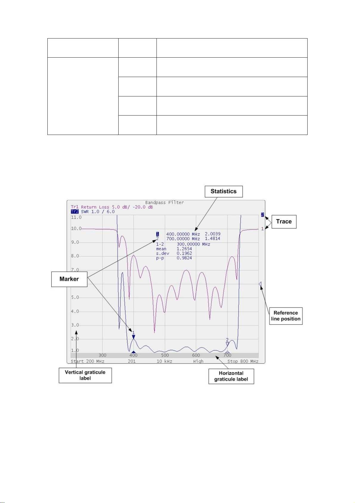
4.2.3 Graph Area
The graph area displays the traces and numeric data (see Figure 4.5).
Figure 4.5 Graph area
46

MEASUREMENT CONDITIONS SETTING
Note
Using the graticule labels, you can easily control all the trace
parameters by the mouse.
The graph area contains the following elements:
Vertical graticule label displays the vertical axis numeric data for the active
trace;
Horizontal graticule label displays stimulus axis numeric data (frequency,
time, or distance);
Reference level position indicates the reference level position of the trace;
Markers indicate the measured values in different points on the active
trace. You can enable display of the markers for all the traces
simultaneously;
Marker functions: statistics, bandwidth, flatness, RF filter;
Trace number allows trace identification in the channel window;
Current stimulus position indication appears when sweep duration exceeds
1 sec.
4.2.4 Markers
The markers indicate the stimulus values and the measured values in selected
points of the trace (see Figure 4.6).
Figure 4.6 Markers
47

MEASUREMENT CONDITIONS SETTING
Symbol
Definition
--
No calibration data. No calibration was performed.
Cor
Error correction is enabled. The stimulus settings are the same for the
measurement and the calibration.
C?
Error correction is enabled. The stimulus settings are not the same for
the measurement and the calibration. Interpolation is applied.
The markers are numbered from 1 to 16. The reference marker is indicated with R
symbol. The active marker is indicated in the following manner: its number is
highlighted in inverse color, the stimulus indicator is fully colored.
4.2.5 Channel Status Bar
The channel status bar is located in the bottom part of the channel window (see
Figure 4.7)
Figure 4.7 Channel status bar
The channel status bar contains the following elements:
Stimulus start field allows to display and enter the start frequency. This
field can be switched to indication of stimulus center frequency, in this
case the word Start will change to Center;
Sweep points field allows to display and enter the number of sweep points.
The number of sweep points can have the following values: 2 - 100001;
IF bandwidth field allows to display and set the IF bandwidth. The values
can be set from 10 Hz to 30 kHz (100 kHz);
Power level field allows to display and enter the port output power;
Stimulus stop field allows to display and enter the stop frequency . This
field can be switched to indication of stimulus span, in this case the word
Stop will change to Span;
Error correction field displays the integrated status of error correction for
S-parameter traces. The values of this field are represented in Table 4.3.
Table 4.3 Error correction field
48

MEASUREMENT CONDITIONS SETTING
Symbol
Definition
C!
Error correction is enabled. The stimulus settings are not the same for
the measurement and the calibration. Extrapolation is applied.
Off
Error correction is turned off.
Note
The manipulations described in this section will help you to
perform the most frequently used settings only. All the channel
functions can be accessed via the softkey menu.
4.3 Quick Channel Setting Using Mouse
This section describes the manipulations, which will enable you to set the channel
parameters of R140 fast and easy. When you move a mouse pointer in the channel
window field where a channel parameter can be changed, the mouse pointer will
change its form and a prompt field will appear.
4.3.1 Active Channel Selection
You can select the active channel window when two or more channel windows
are open. The border line of the active window will be highlighted (see Figure
4.8). To activate a channel click in its window.
Figure 4.8 Active channel window display
49
MEASUREMENT CONDITIONS SETTING
4.3.2 Active Trace Selection
You can select the active trace if the active channel window contains two or more
traces.
The active trace name will be highlighted in inverted color. In the example given
it is Tr2. To activate a trace click on the required trace or its status line.
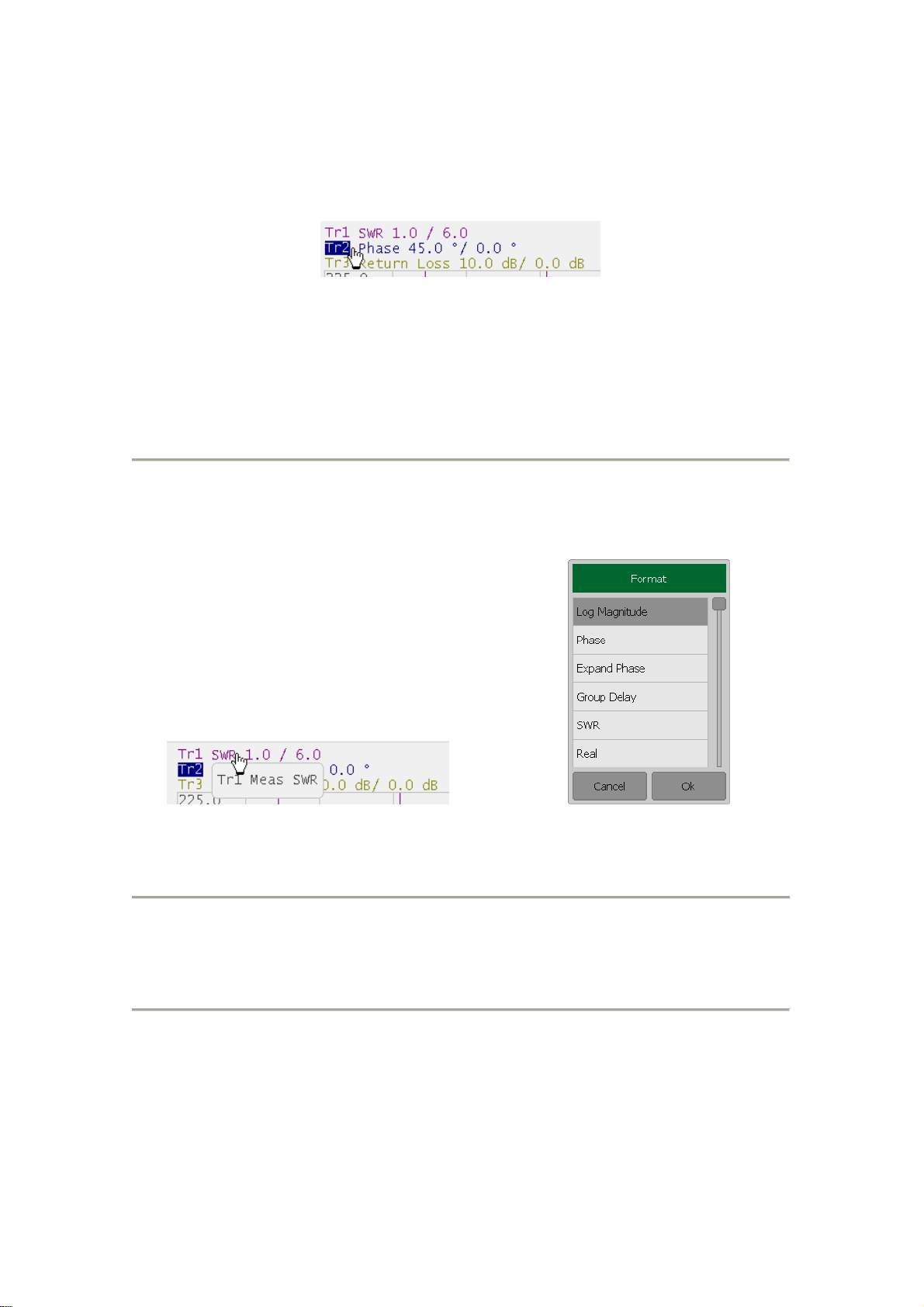
4.3.3 Display Format Setting
To select the trace display format click on the format name in the trace status
line.
Select the required format in the Format dialog and complete the setting by Ok.
4.3.4 Trace Scale Setting
50

MEASUREMENT CONDITIONS SETTING
To select the trace scale click in the trace scale field of the trace status line.
Enter the required numerical value using the on-screen keypad and complete the
setting by Ok.
4.3.5 Reference Level Setting
To set the value of the reference level click on the reference level field in the
trace status line.
Enter the required numerical value using the on-screen keypad and complete the
setting by Ok.
51

MEASUREMENT CONDITIONS SETTING
4.3.6 Marker Stimulus Value Setting
The marker stimulus value can be set by dragging the marker or by entering the
value from the on-screen keypad.
To drag the marker, move the mouse pointer to one of the marker indicators.
The marker will become active, and a pop-up hint with its name will appear near
the marker. The marker can be moved either by dragging its indicator or its hint
area.
To enter the numerical value of the stimulus in the marker data click on the
stimulus value. Then enter the required value using the on-screen keypad.
4.3.7 Switching between Start/Center and Stop/Span Modes
To switch between the modes Start/Center and Stop/Span click in the respective
field of the channel status bar.
Label Start will be replaced by Center, and label Stop will be replaced by Span.
52

MEASUREMENT CONDITIONS SETTING
4.3.8 Start/Center Value Setting
To enter the Start/Center numerical values click on the respective field in the
channel status bar.
Then enter the required value using the on-screen keypad.
4.3.9 Stop/Span Value Setting
To enter the Stop/Span numerical values click on the respective field in the
channel status bar.
Then enter the required value using the on-screen keypad.
53

MEASUREMENT CONDITIONS SETTING
4.3.10 Sweep Points Number Setting
To enter the number of sweep points click in the respective field of the channel
status bar.
Select the required value in the Points dialog and complete the setting by Ok.
4.3.11 IF Bandwidth Setting
To set the IF bandwidth click in the respective field of the channel status bar.
Select the required value in the IFBW dialog and complete the setting by Ok.
54

MEASUREMENT CONDITIONS SETTING
4.3.12 Power Level Setting
To set the output power level click in the respective field of the channel status
bar.
This way you can switch between high and low power settings.
4.4 Channel and Trace Display Setting
The Analyzer supports 4 channels, which allows measurements with different
stimulus parameter settings. The parameters related to a logical channel are listed
in Table 4.4
4.4.1 Setting the Number of Channel Windows
A channel is represented on the screen as an individual channel window. The
screen can display from 1 to 4 channel windows simultaneously. By default one
channel window is opened.
The program supports three options of the channel window layout: one channel,
two channels, and four channels. The channels are allocated on the screen
according to their numbers from left to right and from top to bottom. If there are
more than one channel window on the screen, one of them is selected as active.
The border line of the active window will be highlighted in inverted color.
55

MEASUREMENT CONDITIONS SETTING
Note
For each open channel window, you should set the stimulus
parameters and make other settings.
Before you start channel parameter setting or calibration, you need
to select this channel as active.
To set the number of channel windows displayed on the screen use the following
softkey in the right menu bar Channels. Then select the softkey with the required
number and layout of the channel windows.
In the Active Channel field, you can select the active channel. The repeated
clicking will switch the numbers of all channels.
The measurements are executed for open channel windows in succession.
4.4.2 Channel Activating
Before setting channel parameters, you need to activate the channel.
56

MEASUREMENT CONDITIONS SETTING
To activate the channel use the following softkeys in the right menu bar Channels
> Active Channel.
Active Channel field allows viewing the numbers of all channels from 1 to 4.
Select the required number of the active channel.
To activate a channel, you can also click on its channel window.
4.4.3 Active Channel Window Maximizing
When there are several channel windows displayed, you can temporarily maximize
the active channel window to full screen size.
The other channel windows will be hidden, and this will interrupt the
measurements in those channels.
57

MEASUREMENT CONDITIONS SETTING
Note
Channel maximizing function can be controlled by a double mouse
click on the channel.
To enable/disable active channel maximizing function use the following softkeys
Channel > Maximize Channel.
4.4.4 Number of Traces Setting
Each channel window can contain up to 4 different traces. Each trace is assigned
the display format, scale and other parameters. The parameters related to a trace
are listed in Table 4.5.
The traces can be displayed in one graph, overlapping each other, or in separate
graphs of a channel window. The trace settings are made in two steps: trace
number setting and trace layout setting in the channel window. By default a
channel window contains one trace. If you need to enable two or more traces, set
the number of traces as described below.
58

MEASUREMENT CONDITIONS SETTING
To add a trace use the following softkeys in the right menu bar Trace > Add Trace.
To delete a trace use the following softkeys in the right menu bar Trace > Delete
Trace.
All the traces are assigned their individual names, which cannot be changed. The
trace name contains its number. The trace names are as follows: Tr1, Tr2 ... Tr4.
Each trace is assigned some initial settings: measured parameter, format, scale
and color, which can be modified by the user.
By default the display format for all the traces is set to Return loss (dB).
By default the scale is set to 10 dB, reference level value is set to 0 dB, reference
level position is in the middle of the graph.
The trace color is determined by its number.
4.4.5 Active Trace Selection
Trace parameters can be entered for the active trace. Active trace belongs to the
active channel, and its name is highlighted in inverted color. You have to select
the active trace before setting the trace parameters.
59

MEASUREMENT CONDITIONS SETTING
Note
A trace can be activated by clicking on the trace status bar in the
graphical area of the program
To select the active trace use the softkeys in the right menu bar Trace.
Click the Active Trace to select the trace you want to assign the active.
60

Table 4.4 Channel parameters
N
Parameter Description
1
Sweep Range
2
Number of Sweep Points
3
IF Bandwidth
N
Parameter Description
1
Display Format
2
Reference Level Scale, Value and Position
3
Electrical Delay, Phase Offset
4
Memory Trace
5
Markers
6
Parameter Transformation
Table 4.5 Trace parameters
MEASUREMENT CONDITIONS SETTING
61

MEASUREMENT CONDITIONS SETTING
n Port at waveincident
m Port at wavedtransmitte
=S
mn
4.5 Measurement Parameters Setting
4.5.1 S-Parameters
For high-frequency network analysis the following terms are applied: incident,
reflected and transmitted waves, transferred in the circuits of the setup (see
Figure 4.9).
Figure 4.9
Measurement of magnitude and phase of incident, reflected and transmitted
signals allow to determin the S-parameters (scattered parameters) of the DUT. An
S-parameter is a relation between the complex magnitudes of the two waves:
R140 Analyzer has one measurement port which operates as a signal source and
as a reflected signal receiver. That is why the Analyzer allows measuring only S11
parameter.
4.5.2 Trace Format
The Analyzer offers the display of the measured S-parameters on the screen in
three formats:
rectangular format;
polar format;
Smith chart format.
62
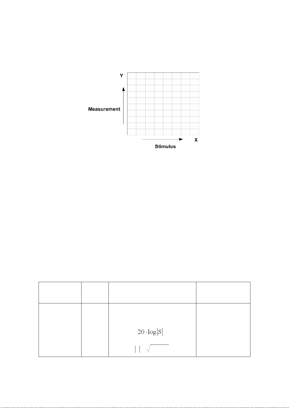
MEASUREMENT CONDITIONS SETTING
bj+a=S
Format Type
Description
Label
Data Type (Y-axis)
Measurement Unit
(Y-axis)
Logarithmic
Magnitude
Log
Mag
S-parameter logarithmic
magnitude:
,
22
baS
Decibel (dB)
4.5.3 Rectangular Format
In this format, stimulus values are plotted along X-axis and the measured data are
plotted along Y-axis (see Figure 4.10).
Figure 4.10 Rectangular format
To display S-parameter complex value along Y-axis, it should be transformed into
a real number. Rectangular formats involve various types of transformation of an
S-parameter
, where:
a – real part of S-parameter complex value;
b – imaginary part of S-parameter complex value.
There are nine types of rectangular formats depending on the measured value
plotted along Y-axis (see Table 4.6).
Table 4.6 Rectangular formats
63

MEASUREMENT CONDITIONS SETTING
Format Type
Description
Label
Data Type (Y-axis)
Measurement Unit
(Y-axis)
Voltage
Standing
Wave Ratio
SWR
Abstract number
Phase
Phase
S-parameter phase from
–180to +180
a
b
arctg
180
Degree (°)
Expanded
Phase
Expand
Phase
S-parameter phase,
measurement range expanded
to from below –180 to over
+180
Degree (°)
Group
Delay
Group
Delay
Signal propagation delay within
the DUT:
d
d
,
a
b
arctg
,
f2
Second (sec.)
Linear
Magnitude
Lin Mag
S-parameter linear magnitude:
Abstract number
Real Part
Real
S-parameter real part:
)(Srea
Abstract number
Imaginary Part
Imag
S-parameter imaginary part:
)(Simb
Abstract number
Cable Loss
Cable
Loss
Decibel (dB)
64

MEASUREMENT CONDITIONS SETTING
Format Type
Description
Label
Data Displayed by Marker
Measurement Unit
(Y-axis)
Linear
Magnitude
and Phase
Polar (Lin)
S-parameter linear magnitude
Abstrac number
S-parameter phase
Degree
Logarithmic
Magnitude
and Phase
Polar (Log)
S-parameter logarithmic
magnitude
Decibel (dB)
S-parameter phase
Degree
Real and
Imaginary
Parts
Polar
(Re/Im)
S-parameter real part
Abstract number
S-parameter imaginary part
Abstract number
4.5.4 Polar Format
Polar format represents the measurement results on the pie chart (see Figure
4.11). The distance to a measured point from the graph center corresponds to the
magnitude of its value. The counterclockwise angle from the positive horizontal
axis corresponds to the phase of the measured value.
Figure 4.11 Polar format
The polar graph does not have a frequency axis, so frequency will be indicated by
the markers. There are three types of polar formats depending on the data
displayed by the marker. The traces will remain the same on all the graphs.
Table 4.7 Polar formats
65

MEASUREMENT CONDITIONS SETTING
Format Type
Description
Label
Data Displayed by Marker
Measurement Unit
(Y-axis)
Linear
Magnitude and
Phase
Smith (Lin)
S-parameter linear
magnitude
Abstract number
S-parameter phase
Degree
Logarithmic
Magnitude and
Phase
Smith (Log)
S-parameter logarithmic
magnitude
Decibel (dB)
S-parameter phase
Degree
Real and
Imaginary
Parts
Smith
(Re/Im)
S-parameter real part
Abstract number
S-parameter imaginary part
Abstract number
4.5.5 Smith Chart Format
Smith chart format is used for representation of impedance values for DUT
reflection measurements. In this format, the trace has the same points as in polar
format.
Figure 4.12 Smith chart format
Smith chart format does not have a frequency axis, so frequency will be indicated
by the markers. There are five types of Smith chart formats depending on the data
displayed by the marker. The traces will remain the same on all the graphs.
Table 4.8 Smith chart format
66

MEASUREMENT CONDITIONS SETTING
Format Type
Description
Label
Data Displayed by Marker
Measurement Unit
(Y-axis)
Complex
Impedance
(at Input)
Smith
(R + jX)
Resistance at input:
)(
inp
ZreR
,
S
S
ZZ
inp
1
1
0
Ohm (Ω)
Reactance at input:
)(
inp
ZimX
Ohm (Ω)
Equivalent capacitance or
inductance:
0,
1
X
X
C
0, X
X
L
Farad (F)
Henry (H)
Complex
admittance
(at Input)
Smith
(G + jB)
Conductance at input:
)(
inp
YreG
,
S
S
Z
Y
inp
1
11
0
Siemens (S)
Susceptance at input:
)(
inp
YimB
Siemens (S)
Equivalent capacitance or
inductance:
0, B
B
C
0,
1
B
B
L
Farad (F)
Henry (H)
Z0 – test port impedance. Z0 setting is described in section 5.2.6
67

MEASUREMENT CONDITIONS SETTING
4.5.6 Data Format Setting
You can select the format for each trace of the channel individually. Before you set
the format, first activate the trace.
To set the trace display format use the following softkey in the right menu bar
Trace.
In the Trace dialog select the required trace from Active Trace and click on
Format.
Then select the required format in the Format dialog. Complete the setting by Ok.
68

MEASUREMENT CONDITIONS SETTING
4.6 Trigger Setting
The trigger mode determines the sweep actuation of the channel at a trigger
signal detection. A channel can operate in one of the following three trigger
modes:
Continuous – a sweep actuation occurs every time a trigger signal is
detected;
Single – one sweep actuation occurs with trigger signal detection after the
mode has been enabled; after the sweep is complete the channel modes
changes to hold;
Hold – sweep actuation is off in the channel, trigger signals do not affect
the channel.
The trigger signal applies to the whole Analyzer and controls the trigging of all
the channels in the following manner. If more than one channel window are open,
the trigger activates successive measurements of all the channels which are not in
hold mode. Before measurement of all channels is complete, all additional triggers
are ignored. When measurement of all the channels is complete, if there is as least
one channel in continuous trigger mode, the Analyzer will enter waiting for a
trigger state.
The trigger source can be selected by the user from the following four available
options:
Internal – the next trigger signal is generated by the Analyzer on
completion of each sweep;
External – the external trigger input is used as a trigger signal source
(except R54);
Bus – the trigger signal is generated by a command communicated from an
external computer from a program controlling the Analyzer via COM/DCOM.
To set the trigger mode, use the following softkeys Trigger > Trigger Mode.
69

Then select the required trigger mode:
Hold
Single
Continuous
MEASUREMENT CONDITIONS SETTING
To set the trigger source, use the following softkeys Trigger > Trigger Source.
Then select the required trigger source:
Internal
External
Bus
70

MEASUREMENT CONDITIONS SETTING
4.6.1 External Trigger (except R54)
4.6.1.1 Point Feature
By default the external trigger initiates a sweep measurement upon every trigger
event (See Figure 4.13 a, b). For the external trigger source, the point trigger
feature instead initiates a point measurement upon each trigger event (See Figure
4.13 c, d).
To enable the point trigger feature for external trigger source, use the following
softkeys Trigger > Trigger Input > Event { On Sweep | On Point }.
4.6.1.2 External Trigger Polarity
71

MEASUREMENT CONDITIONS SETTING
To select the external trigger polarity, use the following softkeys Trigger > Trigger
Input > Polarity { NegativeEdge | Positive Edge }.
4.6.1.3 External Trigger Position
The external trigger position selects the position when Analyzer expects the
external trigger signal:
Before sampling, when the frequency of the stimulus port have been set.
The frequency change of the stimulus port begins after sampling (See
Figure 4.13 a, c).
Before the frequency setup and subsequent measurement. The frequency
change of the stimulus port begins when the external trigger arrives (See
Figure 4.13 b, d).
Depending on the Point Feature settings the external trigger is expected before
each point or before the first point of the full sweep cycle.
72

MEASUREMENT CONDITIONS SETTING
To select external trigger polarity, use the following softkeys: Trigger > Trigger
Input > Position { Before Sampling | Before Setup }.
4.6.1.4 External Trigger Delay
The external trigger delay sets the response delay with respect to the external
trigger signal (see Figure 4.13). The delay value has range from 0 to 100 sec with
resolution 0.1 μsec.
To set the external trigger delay, use the following softkeys: Trigger > Trigger
Input > Delay.
73

MEASUREMENT CONDITIONS SETTING
74

MEASUREMENT CONDITIONS SETTING
Figure 4.13 External Trigger
75

MEASUREMENT CONDITIONS SETTING
4.6.2 Trigger Output (except R54/R140)
The trigger output outputs various waveforms depending on the setting of the
Output Trigger Function:
Before frequency setup pulse;
Before sampling pulse;
After sampling pulse;
Ready for external trigger;
End of sweep pulse;
Measurement sweep.
Figure 4.14 Trigger Output (except Ready for Trigger)
Figure 4.15 Trigger Output (Ready for Trigger)
76

MEASUREMENT CONDITIONS SETTING
Note
When the Ready for Trigger function of the trigger output is
selected the trigger source must be set to external to enable the
output trigger.
4.6.2.1 Switching ON/OFF Trigger Output
To enable/disable the trigger output, use the following softkeys Trigger > Trigger
Output > Enable Out.
77
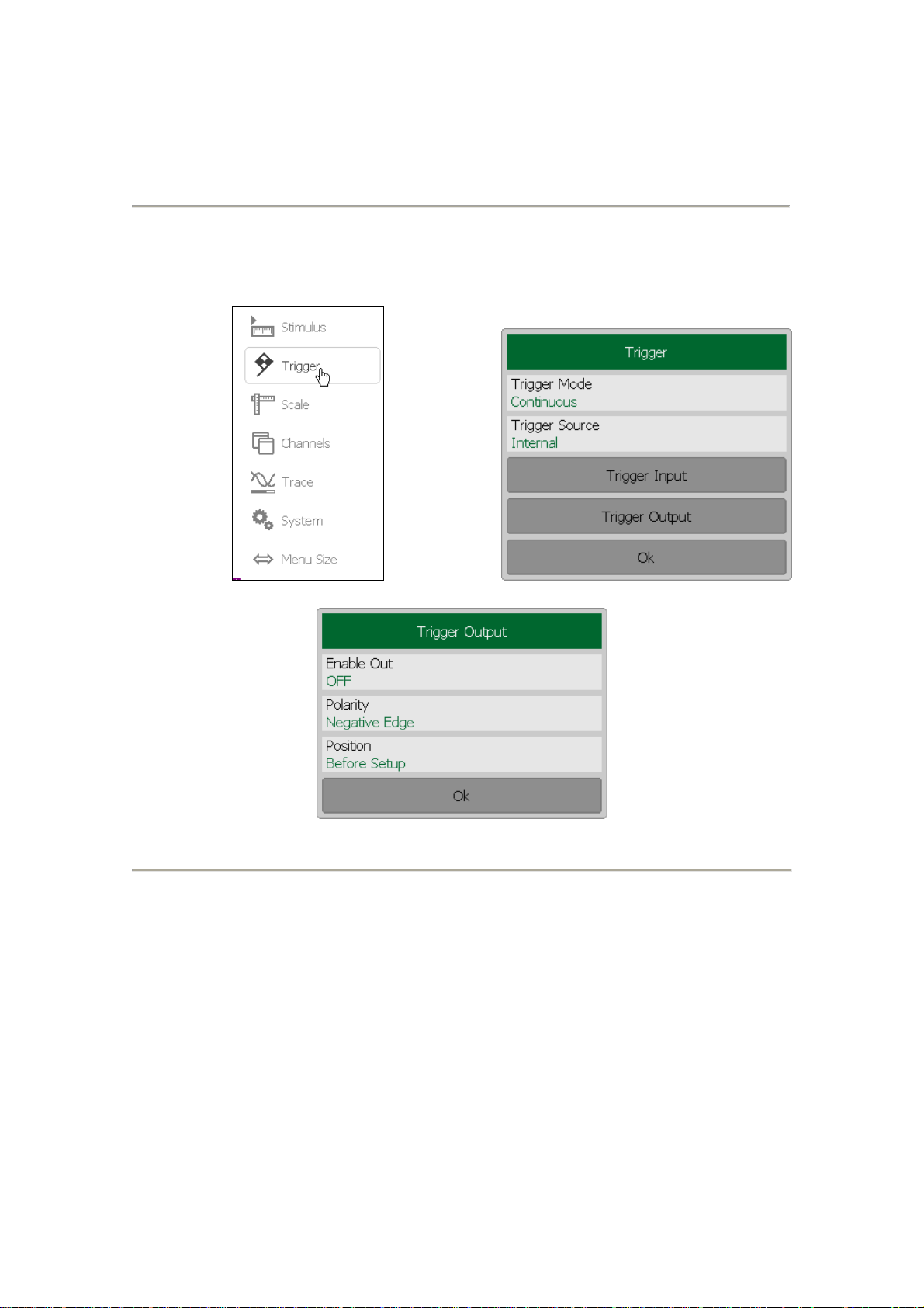
MEASUREMENT CONDITIONS SETTING
4.6.2.2 Trigger Output Polarity
To select the polarity of the trigger output, use the following softkeys Trigger >
Trigger Output > Polarity { NegativeEdge | Positive Edge }.
78

MEASUREMENT CONDITIONS SETTING
4.6.2.3 Trigger Output Function
To select the function of the trigger output (See Figure 4.14, Figure 4.15), use the
following softkeys Trigger > Trigger Output > Position { Before Setup |
BeforeSampling | After Sampling | Ready for Trigger | Sweep End | Measurement }.
79

MEASUREMENT CONDITIONS SETTING
4.7 Scale Setting
4.7.1 Rectangular Scale
For rectangular format you can set the following parameters (see Figure 4.16):
Trace scale;
Reference level value;
Reference level position;
Number of scale divisions.
Figure 4.16 Rectangular scale
4.7.2 Rectangular Scale Setting
You can set the scale for each trace of a channel. Before you set the scale, first
activate the trace.
To set the scale of a trace use the following softkey in the right menu bar Scale.
80

MEASUREMENT CONDITIONS SETTING
Then select the Scale field and enter the required value using the on-screen
keypad.
To set the reference level select the Ref. Value field and enter the required value
using the on-screen keypad.
To set the position of the reference level select the Ref. Position field and enter
the required value using the on-screen keypad.
To set the number of trace scale divisions1 select the Divisions field and enter the
required value using the on-screen keypad.
4.7.3 Circular Scale
For polar and Smith chart format, you can set the outer circle value (see Figure
4.17).
Figure 4.17 Circular scale
4.7.4 Circular Scale Setting
1 The number of scale divisions affects all channel traces.
81

MEASUREMENT CONDITIONS SETTING
To set the scale of the circular graph use the following softkey in the right menu
bar Scale.
Then select the Scale field and enter the required value using the on-screen
keypad.
4.7.5 Automatic Scaling
The automatic scaling function allows the user to define the trace scale
automatically so that the trace of the measured value could fit into the graph
entirely.
In rectangular format, two parameters are adjustable: scale and reference level
position. In circular format, the outer circle value will be adjusted.
To execute the automatic scaling use the following softkeys in the right menu bar
Scale > Auto Scale.
82

MEASUREMENT CONDITIONS SETTING
tfj
eS=S
π2
4.7.6 Reference Level Automatic Selection
This function executes automatic selection of the reference level in rectangular
coordinates.
After the function has been executed, the trace of the measured value makes the
vertical shift so that the reference level crosses the graph in the middle. The scale
will remain the same.
To execute the automatic selection of the reference level use the following
softkeys in the right menu bar Scale > Auto Ref. Value.
4.7.7 Electrical Delay Setting
The electrical delay function allows the user to define the compensation value for
the electrical delay of a device. This value is used as compensation for the
electrical delay during non-linear phase measurements. The electrical delay is set
in seconds.
If the electrical delay setting is other than zero, S-parameter value will vary in
accordance with the following formula:
, where
f – frequency, Hz,
t – electrical delay, sec.
83
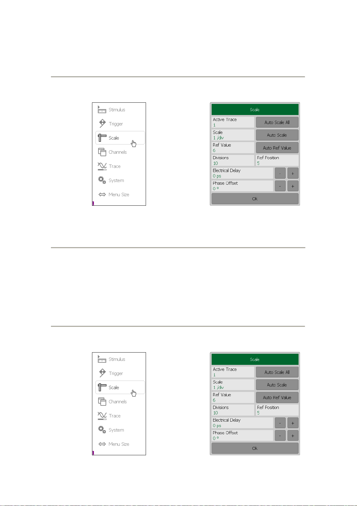
MEASUREMENT CONDITIONS SETTING
The electrical delay is set for each trace individually. Before you set the electrical
delay, first activate the trace.
To set the electrical delay use the following softkey in the right menu bar Scale.
Then select the Electrical Delay field and enter the required value using the onscreen keypad.
4.7.8 Phase Offset Setting
The phase offset function allows the user to define the constant phase offset of a
trace. The value of the phase offset is set in degrees for each trace individually. To
set the phase offset, first activate the trace.
To set the phase offset use the following softkey in the right menu bar Scale.
84

MEASUREMENT CONDITIONS SETTING
Then select the Phase Offset field and enter the required value using the on-
screen keypad.
85

MEASUREMENT CONDITIONS SETTING
Note
If you select segment frequency sweep, the Segment Table softkey
will be become available in Stimulus dialog. For segment tables
details see section 4.8.5.
4.8 Stimulus Setting
The stimulus parameters are set for each channel. Before you set the stimulus
parameters of a channel, make this channel active.
4.8.1 Sweep Type Setting
To set the sweep type use the following softkey in the right menu bar Stimulus.
4.8.2 Sweep Span Setting
86

MEASUREMENT CONDITIONS SETTING
To enter the start and stop values of the sweep range use the following softkey in
the right menu bar Stimulus.
Then select the Start Frequency or Stop Frequency field and enter the required
values using the on-screen keypad.
If necessary, you can select the measurement units. The current measurement
units are shown to the right from the value entry field.
4.8.3 Sweep Points Setting
To enter the number of sweep points use the following softkey in the right menu
bar Stimulus.
87

MEASUREMENT CONDITIONS SETTING
Then click on Points field, select the required value from the list and complete the
setting by Ok.
4.8.4 Stimulus Power Setting
The stimulus power level can take two possible values. High output power
corresponds to the source signal power of -10 dB/m. Low output power
corresponds to -30 dBm.
To enter the power level value use the following softkeys in the right menu bar
Stimulus > Power.
Then select the Output power field to switch between the high and low settings
of the power level.
The set power level can also be seen in the channel status bar.
4.8.5 Segment Table Editing
Frequency sweep span can be divided into segments. Each segment has start and
stop values of the sweep range, number of points and measurement delay. IF filter
and measurement delay can be enabled/disabled by the user.
88

MEASUREMENT CONDITIONS SETTING
The types of segment tables are shown below.
Each table line determines one segment. The table can contain one or several
lines. The number of lines is limited by the aggregate number of all segment
points, i.e. 100001
To edit the segment table use the following softkeys in the right menu bar
Stimulus > Segment Table.
Select the segment frequency sweep to make the Segment Table softkey available
(see section 4.8.1).
To add a segment to the segment table use Add.
To delete a segment from the table use Delete.
89

MEASUREMENT CONDITIONS SETTING
Note
The adjacent segments cannot overlap in the frequency domain.
To enter the segment parameters, move the mouse to the respective box and
enter the numerical value. You can navigate the segment table using the «Up
Arrow», «Down Arrow », «Left Arrow », «Right Arrow» keys.
To edit any parameter in the table, double click on the its value field and enter
the required value using the on-screen keypad.
To enable/disable the IFBW filter column click on the List IFBW field.
To enable/disable the measurement delay column click on the List Delay field.
The segment table can be saved into *.seg file to a hard disk and later recalled.
To save the segment table use Save.
To recall the segment table use Recall.
90

MEASUREMENT CONDITIONS SETTING
4.9 Trigger Setting
The Analyzer can operate in one of three sweep trigger modes. The trigger mode
determines the sweep actuation. The trigger can have the following modes:
Continuous – a sweep actuation occurs every time after sweep cycle is
complete in each channel;
Single – sweep actuation occurs once, and after the sweep is complete, the
trigger turns to hold mode;
Hold – sweep is stopped, the actuation does not occur.
If more than one channel window is displayed on the screen, a sweep will be
actuated in them in succession.
Trigger source can be internal or bus (transferred through COM/DCOM).
To set the trigger mode use the following softkey in the right menu bar Trigger.
Then click on Trigger Mode field select the required mode from the list and
complete the setting by Ok.
Close the Trigger dialog by Ok.
If you select Single Trigger Mode you can actuate sweep by clicking on the
Trigger Event softkey in the right menu bar.
91

MEASUREMENT CONDITIONS SETTING
4.10 Measurement Optimizing
4.10.1 IF Bandwidth Setting
The IF bandwidth function allows the user to define the bandwidth of the test
receiver. The IF bandwidth can be selected by user from the following values: 100
Hz, 300 Hz, 1 kHz, 3 kHz, 10 kHz and 30 kHz.
The IF bandwidth narrowing allows you to reduce self-noise and widen the
dynamic range of the Analyzer. Also the sweep time will increase. Narrowing of
the IF bandwidth to 10 will reduce the receiver noise to 10 dB.
The IF bandwidth should be set for each channel individually. Before you set the
IF bandwidth, first activate the channel.
To set the IF bandwidth use the following softkey in the left menu bar Average.
To set the IF bandwidth click on IFBW field and select the required value from the
list. Complete the setting by Ok.
4.10.2 Averaging Setting
The averaging function is similar to IF bandwidth narrowing, it allows reducing
self-noise and widening the dynamic range of the Analyzer.
The averaging in each measurement point is made over several sweeps according
to the exponential window method.
The averaging should be set for each channel individually. Before you set the
averaging, first activate the channel.
92

MEASUREMENT CONDITIONS SETTING
To set the averaging use the following softkey in the left menu bar Average.
To toggle the averaging function on/off click on Average field.
To set the averaging factor click on Averaging Factor field and enter the required
value using the on-screen keypad.
4.10.3 Smoothing Setting
The smoothing of the sweep results is made by averaging the measurement
results of adjacent points of the trace determined by the moving aperture. The
aperture is set by the user in percent from the total number of the trace points.
The smoothing does not increase the dynamic range of the Analyzer. It preserves
the average level of the trace and reduces the noise bursts.
The smoothing should be set for each trace individually. To set the smoothing,
first activate the trace.
93

MEASUREMENT CONDITIONS SETTING
To set the smoothing use the following softkey in the left menu bar Average.
To toggle the smoothing function on/off click on Smoothing field.
To set the smoothing aperture click on Smoothing Aperture field and enter the
required value using the on-screen keypad.
94

MEASUREMENT CONDITIONS SETTING
4.10.4 Trace Hold Function
The Trace Hold function displays the maximum or the minimum of any given
active measurement instead the real-time data. The held data is displayed as an
active trace.
To toggle the Trace Hold function on/off use the following softkeys in the right
menu bar Trace > Trace Hold.
Then select the required type (Maximum | Minimum) from the Hold Type list and
complete the setting by Ok.
95

MEASUREMENT CONDITIONS SETTING
4.11 Cable Specifications
By default, the program does NOT compensate DTF measurements to account for
the inherent loss of a cable. However, to make more accurate DTF measurements,
the cable loss and velocity factor can be entered using one of the following
methods:
Select a cable type from a list which contains the Cable loss in dB/meter
and Velocity factor;
Manually enter Cable loss and Velocity factor for the measurement.
Velocity factor is a property of the physical material of a cable. A VF of 1.0
corresponds to the speed of light in a vacuum, or the fastest VF possible. A
polyethylene dielectric cable has VF = 0.66 and a cable with Teflon dielectric has
VF = 0.7.
Cable Loss is specified in dB/meter. In addition to the length of the cable, loss is
also directly proportional to the frequency of the signal that passes through the
cable.
4.11.1 Selecting the type of cable
To select the type of cable use the following softkeys in the left menu bar
Analysis > Time Domain > Cable Correction > Cable type.
96

MEASUREMENT CONDITIONS SETTING
Select the required item from the Cable List and complete the setting by Ok
4.11.2 Manually specify Velocity Factor and Cable Loss
To set the parameters of cable, press the following softkeys in the left menu bar
Analysis > Time Domain > Cable Correction.
97

MEASUREMENT CONDITIONS SETTING
Click on Velocity Factor field to enter the value of velocity factor using the onscreen keypad.
Click on Loss field to enter the value of cable loss using the on-screen keypad.
4.11.3 Editing table of cables
To edit the table of cables, press the following softkeys in the left menu bar
Analysis > Time Domain > Cable Correction.
98

MEASUREMENT CONDITIONS SETTING
Click the left button of the mouse on the field Cable Type.
To add/delete rows in the table click Add/Delete.
Then select the required parameter in the table and double click on the
corresponding cell.
Enter the required value Cable Name, Velocity, Cable Loss etc using the on-screen
keypad.
To save the table of cables on the drive click the Save Cable List button.
To restore the table cables from the drive, press the Restore Cable List softkey.
99

5. CALIBRATION AND CALIBRATION KIT
5.1 General Information
5.1.1 Measurement Errors
S-parameter measurements are influenced by various measurement errors, which
can be devided into two categories:
systematic errors,
random errors.
Random errors comprise such errors as noise fluctuations and thermal drift in
electronic components, changes in the mechanical dimensions of connectors
subject to temperature drift, repeatability of connections. Random errors are
unpredictable and hence cannot be estimated and eliminated in calibration.
Random errors can be reduced by correct setting of the source power, IF
bandwidth narrowing, maintaining constant environment temperature, observance
of the Analyzer warm-up time, careful connector handling, avoidance of cable
bending after calibration, and use of the calibrated torque wrench for connection
of the Male-Female coaxial RF connectors.
Random errors and related methods of correction are not mentioned further in
this section.
Systematic errors are the errors caused by imperfections in the components of the
measurement system. Such errors occur repeatedly and their characteristics do not
change with time. Systematic errors can be determined and then reduced by
performing mathematical correction of the measurement results.
The process of measurement of precision devices with predefined parameters with
the purpose of determination of measurement systematic errors is called
calibration, and such precision devices are called calibration standards. The most
commonly used calibration standards are SHORT, OPEN, and LOAD.
The process of mathematical compensation (numerical reduction) for
measurement systematic errors is called an error correction.
5.1.2 Systematic Errors
The systematic measurement errors of vector network analyzers are subdivided
into the following categories according to their source:
Directivity;
Source match;
Reflection tracking.
100
 Loading...