Cisco GS7000 User Manual

Cisco 1.2 GHz GS7000 Node

Installation and Operation Guide

For Your Safety

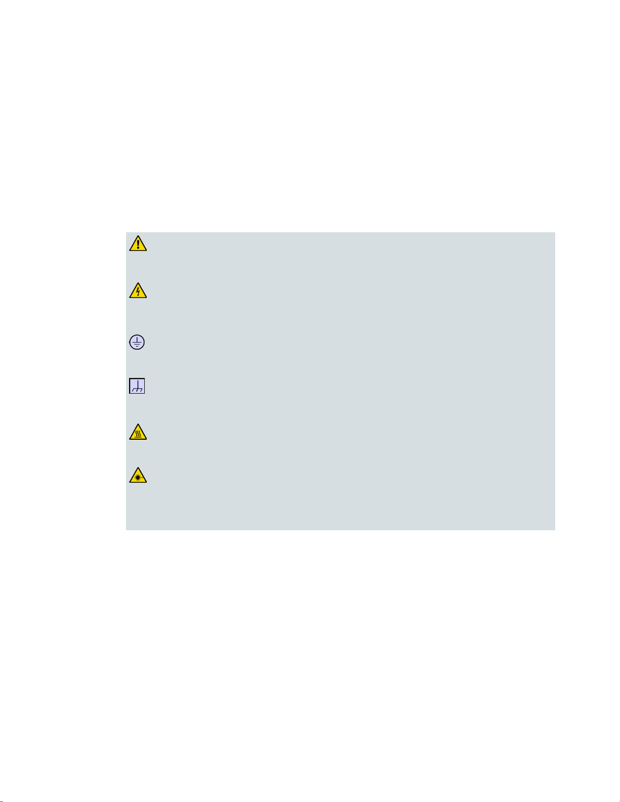
You may find this symbol in the document that accompanies this product. This symbol indicates important operating or maintenance instructions.

You may find this symbol affixed to the product. This symbol indicates a live terminal where a dangerous voltage may be present; the tip of the flash points to the terminal device.

You may find this symbol affixed to the product. This symbol indicates a protective ground terminal.

You may find this symbol affixed to the product. This symbol indicates a chassis terminal (normally used for equipotential bonding).

You may find this symbol affixed to the product. This symbol warns of a potentially hot surface.

You may find this symbol affixed to the product and in this document. This symbol indicates an infrared laser that transmits intensity-modulated light and emits invisible laser radiation or an LED that transmits intensity-modulated light.

Explanation of Warning and Caution Icons

Avoid personal injury and product damage! Do not proceed beyond any symbol until you fully understand the indicated conditions.

The following warning and caution icons alert you to important information about the safe operation of this product:

Important

Please read this entire guide. If this guide provides installation or operation instructions, give particular attention to all safety statements included in this guide.

Notices

Trademark Acknowledgments

Cisco and the Cisco logo are trademarks or registered trademarks of Cisco and/or its affiliates in the U.S. and other countries. To view a list of Cisco trademarks, go to this URL: http://www.cisco.com/go/trademarks.

Third party trademarks mentioned are the property of their respective owners.

The use of the word partner does not imply a partnership relationship between Cisco and any other company. (1110R)

Publication Disclaimer

Cisco Systems, Inc. assumes no responsibility for errors or omissions that may appear in this publication. We reserve the right to change this publication at any time without notice. This document is not to be construed as conferring by implication, estoppel, or otherwise any license or right under any copyright or patent, whether or not the use of any information in this document employs an invention claimed in any existing or later issued patent.

Information in this publication is subject to change without notice. No part of this publication may be reproduced or transmitted in any form, by photocopy, microfilm, xerography, or any other means, or incorporated into any information retrieval system, electronic or mechanical, for any purpose, without the express permission of Cisco Systems, Inc.

iii

Contents

For Your Safety ......................................................................................................................... 3

Notices ....................................................................................................................................... 4

Important Safety Instructions.............................................................................................. vii

Laser Safety ............................................................................................................................xiii

Laser Warning Labels ............................................................................................................ xv

General Information 1

Equipment Description ........................................................................................................... 2

Theory of Operation 15

System Diagrams ................................................................................................................... 17

Forward Path .......................................................................................................................... 21

Reverse Path ........................................................................................................................... 22

Power Distribution ................................................................................................................ 23

RF Amplifier Module ............................................................................................................ 24

Forward Configuration Module .......................................................................................... 29

Reverse Configuration Module ............................................................................................ 34

Optical Interface Board (OIB) ............................................................................................... 38

Optical Receiver Module ...................................................................................................... 39

Optical Analog Transmitter Modules ................................................................................. 43

Optical Amplifier (EDFA) Modules .................................................................................... 45

Optical Switch Module .......................................................................................................... 52

Local Control Module ........................................................................................................... 58

Power Supply Module .......................................................................................................... 61

Installation 65

Tools and Test Equipment .................................................................................................... 66

Node Housing Ports .............................................................................................................. 68

Strand Mounting the Node ................................................................................................... 69

Pedestal or Wall Mounting the Node ................................................................................. 72

Fiber Optic Cable Installation .............................................................................................. 74

RF Cable Installation ............................................................................................................. 82

Applying Power to the Node ............................................................................................... 85

Setup and Operation 89

Tools and Test Equipment .................................................................................................... 90

System Diagrams ................................................................................................................... 91

Forward Path Setup Procedure ............................................................................................ 97

Contents

Reverse Path Setup Procedure ........................................................................................... 101

Reconfiguring Forward Signal Routing ............................................................................ 103

Reconfiguring Reverse Signal Routing ............................................................................. 113

Maintenance 121

Opening and Closing the Housing .................................................................................... 122

Preventative Maintenance .................................................................................................. 124

Removing and Replacing Modules ................................................................................... 127

Care and Cleaning of Optical Connectors ........................................................................ 134

Troubleshooting 139

No RF Output at Receiver RF Test Point: Optical Power LED on Receiver Module is

off ........................................................................................................................................... 140

No RF Output: Fiber Optic Light Level is Good, Receiver Optical Power LED is on 142

Poor C/N Performance ....................................................................................................... 144

Poor Distortion Performance .............................................................................................. 146

Poor Frequency Response ................................................................................................... 148

No RF Output from Reverse Receiver .............................................................................. 150

Customer Support Information 151

Appendix A Technical Information 153

Linear Tilt Chart ................................................................................................................... 154

Forward Equalizer Chart .................................................................................................... 156

Appendix B Enhanced Digital Return Multiplexing Applications 158

Enhanced Digital Return System Overview .................................................................... 159

Enhanced Digital Return (EDR) System Installation ...................................................... 177

Transmitter Module Setup Procedure .............................................................................. 186

Reverse Balancing the Node with EDR ............................................................................ 189

Troubleshooting ................................................................................................................... 192

Appendix C Expanded Fiber Tray 197

Expanded Fiber Tray Overview......................................................................................... 198

Expanded Fiber Tray Installation ...................................................................................... 200

Fiber Management System ................................................................................................. 203

Configuration Examples ..................................................................................................... 209

Contents

Glossary 213

Index 225

Important Safety Instructions

vii

Important Safety Instructions

WARNING:

To reduce risk of electric shock, perform only the instructions that are included in the operating instructions. Refer all servicing to qualified service personnel only.

Read and Retain Instructions

Carefully read all safety and operating instructions before operating this equipment, and retain them for future reference.

Follow Instructions and Heed Warnings

Follow all operating and use instructions. Pay attention to all warnings and cautions in the operating instructions, as well as those that are affixed to this equipment.

Terminology

The terms defined below are used in this document. The definitions given are based on those found in safety standards.

Service Personnel - The term service personnel applies to trained and qualified individuals who are allowed to install, replace, or service electrical equipment. The service personnel are expected to use their experience and technical skills to avoid possible injury to themselves and others due to hazards that exist in service and restricted access areas.

User and Operator - The terms user and operator apply to persons other than service personnel.

Ground(ing) and Earth(ing) - The terms ground(ing) and earth(ing) are synonymous. This document uses ground(ing) for clarity, but it can be interpreted as having the same meaning as earth(ing).

Electric Shock Hazard

This equipment meets applicable safety standards.

Electric shock can cause personal injury or even death. Avoid direct contact with dangerous voltages at all times.

Know the following safety warnings and guidelines:

 Only qualified service personnel are allowed to perform equipment installation

Important Safety Instructions

viii

or replacement.

WARNING:

Avoid personal injury and damage to this equipment. An unstable mounting surface may cause this equipment to fall.

CAUTION:

Be aware of the size and weight of strand-mounted equipment during the installation operation.

Ensure that the strand can safely support the equipment’s weight.

WARNING:

Avoid the possibility of personal injury. Ensure proper handling/lifting techniques are employed when working in confined spaces with heavy equipment.

 Only qualified service personnel are allowed to remove chassis covers and access

any of the components inside the chassis.

Equipment Placement

To protect against equipment damage or injury to personnel, comply with the following:

 Install this equipment in a restricted access location (access restricted to service

personnel).

 Make sure the mounting surface or rack is stable and can support the size and

weight of this equipment.

Strand (Aerial) Installation

Pedestal, Service Closet, Equipment Room or Underground Vault Installation

 Ensure this equipment is securely fastened to the mounting surface or rack

where necessary to protect against damage due to any disturbance and subsequent fall.

 Ensure the mounting surface or rack is appropriately anchored according to

manufacturer’s specifications.

 Ensure the installation site meets the ventilation requirements given in the

equipment’s data sheet to avoid the possibility of equipment overheating.

 Ensure the installation site and operating environment is compatible with the

equipment’s International Protection (IP) rating specified in the equipment’s data

sheet.

Important Safety Instructions

Connection to Network Power Sources

CAUTION:

RF connectors and housing seizure assemblies can be damaged if shunts are not removed from the equipment before installing or removing modules from the housing.

WARNING:

Avoid electric shock! Opening or removing this equipment’s cover may

expose you to dangerous voltages.

CAUTION:

These servicing precautions are for the guidance of qualified service personnel only. To reduce the risk of electric shock, do not perform any servicing other than that contained in the operating instructions unless you are qualified to do so. Refer all servicing to qualified service personnel.

Refer to this equipment’s specific installation instructions in this manual or in

companion manuals in this series for connection to network ferro-resonant AC power sources.

AC Power Shunts

AC power shunts may be provided with this equipment.

Important: The power shunts (where provided) must be removed before installing modules into a powered housing. With the shunts removed, power surge to the components and RF-connectors is reduced.

Equipotential Bonding

If this equipment is equipped with an external chassis terminal marked with the IEC

60417-5020 chassis icon ( ), the installer should refer to CENELEC standard EN 50083-1 or IEC standard IEC 60728-11 for correct equipotential bonding connection instructions.

General Servicing Precautions

Be aware of the following general precautions and guidelines:

 Servicing - Servicing is required when this equipment has been damaged in any

way, such as power supply cord or plug is damaged, liquid has been spilled or objects have fallen into this equipment, this equipment has been exposed to rain or moisture, does not operate normally, or has been dropped.

Important Safety Instructions

 Wristwatch and Jewelry - For personal safety and to avoid damage of this

equipment during service and repair, do not wear electrically conducting objects such as a wristwatch or jewelry.

 Lightning - Do not work on this equipment, or connect or disconnect cables,

during periods of lightning.

 Labels - Do not remove any warning labels. Replace damaged or illegible

warning labels with new ones.

 Covers - Do not open the cover of this equipment and attempt service unless

instructed to do so in the instructions. Refer all servicing to qualified service personnel only.

 Moisture - Do not allow moisture to enter this equipment.  Cleaning - Use a damp cloth for cleaning.  Safety Checks - After service, assemble this equipment and perform safety

checks to ensure it is safe to use before putting it back into operation.

Electrostatic Discharge

Electrostatic discharge (ESD) results from the static electricity buildup on the human body and other objects. This static discharge can degrade components and cause failures.

Take the following precautions against electrostatic discharge:

 Use an anti-static bench mat and a wrist strap or ankle strap designed to safely

ground ESD potentials through a resistive element.

 Keep components in their anti-static packaging until installed.  Avoid touching electronic components when installing a module.

Batteries

This product may contain batteries. Special instructions apply regarding the safe use and disposal of batteries:

Safety

 Insert batteries correctly. There may be a risk of explosion if the batteries are

incorrectly inserted.

 Do not attempt to recharge ‘disposable’ or ‘non-reusable’ batteries.  Please follow instructions provided for charging ‘rechargeable’ batteries.  Replace batteries with the same or equivalent type recommended by

manufacturer.

Important Safety Instructions

 Do not expose batteries to temperatures above 100°C (212°F).

Disposal

 The batteries may contain substances that could be harmful to the environment  Recycle or dispose of batteries in accordance with the battery manufacturer’s

instructions and local/national disposal and recycling regulations.

 The batteries may contain perchlorate, a known hazardous substance, so special

handling and disposal of this product might be necessary. For more information about perchlorate and best management practices for perchlorate-containing substance, see www.dtsc.ca.gov/hazardouswaste/perchlorate.

Modifications

This equipment has been designed and tested to comply with applicable safety, laser safety, and EMC regulations, codes, and standards to ensure safe operation in its intended environment. Refer to this equipment's data sheet for details about regulatory compliance approvals.

Do not make modifications to this equipment. Any changes or modifications could void the user’s authority to operate this equipment.

Modifications have the potential to degrade the level of protection built into this equipment, putting people and property at risk of injury or damage. Those persons making any modifications expose themselves to the penalties arising from proven non-compliance with regulatory requirements and to civil litigation for compensation in respect of consequential damages or injury.

Accessories

Use only attachments or accessories specified by the manufacturer.

Electromagnetic Compatibility Regulatory Requirements

This equipment meets applicable electromagnetic compatibility (EMC) regulatory requirements. Refer to this equipment's data sheet for details about regulatory compliance approvals. EMC performance is dependent upon the use of correctly shielded cables of good quality for all external connections, except the power source, when installing this equipment.

 Ensure compliance with cable/connector specifications and associated

installation instructions where given elsewhere in this manual.

Important Safety Instructions

xii

EMC Compliance Statements

Where this equipment is subject to USA FCC and/or Industry Canada rules, the following statements apply:

FCC Statement for Class A Equipment

This equipment has been tested and found to comply with the limits for a Class A digital device, pursuant to Part 15 of the FCC Rules. These limits are designed to provide reasonable protection against harmful interference when this equipment is operated in a commercial environment.

This equipment generates, uses, and can radiate radio frequency energy and, if not installed and used in accordance with the instruction manual, may cause harmful interference to radio communications. Operation of this equipment in a residential area is likely to cause harmful interference in which case users will be required to correct the interference at their own expense.

Industry Canada - Industrie Canadiene Statement

This apparatus complies with Canadian ICES-003. Cet appareil est confome à la norme NMB-003 du Canada.

CENELEC/CISPR Statement with Respect to Class A Information Technology Equipment

This is a Class A equipment. In a domestic environment this equipment may cause radio interference in which case the user may be required to take adequate measures.

Laser Safety

xiii

Laser Safety

WARNING:



Avoid personal injury! Use of controls, adjustments, or procedures other than those specified herein may result in hazardous radiation exposure.



Avoid personal injury! The laser light source on this equipment (if a transmitter) or the fiber cables connected to this equipment emit invisible laser radiation. Avoid direct exposure to the laser light source.



Avoid personal injury! Viewing the laser output (if a transmitter) or fiber cable with optical instruments (such as eye loupes, magnifiers, or microscopes) may pose an eye hazard.

WARNING:

Avoid personal injury! Qualified service personnel may only perform the procedures in this manual. Wear safety glasses and use extreme caution when handling fiber optic cables, particularly during splicing or terminating operations. The thin glass fiber core at the center of the cable is fragile when exposed by the removal of cladding and buffer material. It easily fragments into glass splinters. Using tweezers, place splinters immediately in a sealed waste container and dispose of them safely in accordance with local regulations.

Introduction

This equipment contains an infrared laser that transmits intensity-modulated light and emits invisible radiation.

Warning: Radiation

 Do not apply power to this equipment if the fiber is unmated or unterminated.  Do not stare into an unmated fiber or at any mirror-like surface that could reflect

light emitted from an unterminated fiber.

 Do not view an activated fiber with optical instruments (e.g., eye loupes,

magnifiers, microscopes).

 Use safety-approved optical fiber cable to maintain compliance with applicable

laser safety requirements.

Warning: Fiber Optic Cables

Laser Safety

xiv

Safe Operation for Software Controlling Optical Transmission

WARNING:



Ensure that all optical connections are complete or terminated before using this equipment to remotely control a laser device. An optical or laser device can pose a hazard to remotely located personnel when operated without their knowledge.



Allow only personnel trained in laser safety to operate this software. Otherwise, injuries to personnel may occur.



Restrict access of this software to authorized personnel only.



Install this software in equipment that is located in a restricted access area.

Equipment

If this manual discusses software, the software described is used to monitor and/or

control ours and other vendors’ electrical and optical equipment designed to

transmit video, voice, or data signals. Certain safety precautions must be observed when operating equipment of this nature.

For equipment specific safety requirements, refer to the appropriate section of the equipment documentation.

For safe operation of this software, refer to the following warnings.

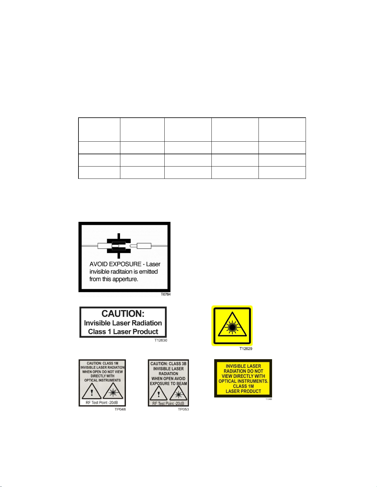
Laser Warning Labels

Output Power

Maximum Output

CDRH Classification

IEC 60825-1 Classification

IEC 60825-2 Hazard Level

17 dBm

20 dBm

22 dBm

Maximum Laser Power

The maximum laser power that can be expected from the EDFA optical amplifier for various amplifier configurations is defined in the following table.

Warning Labels

One or more of the labels shown below are located on this product.

Laser Warning Labels

xvi

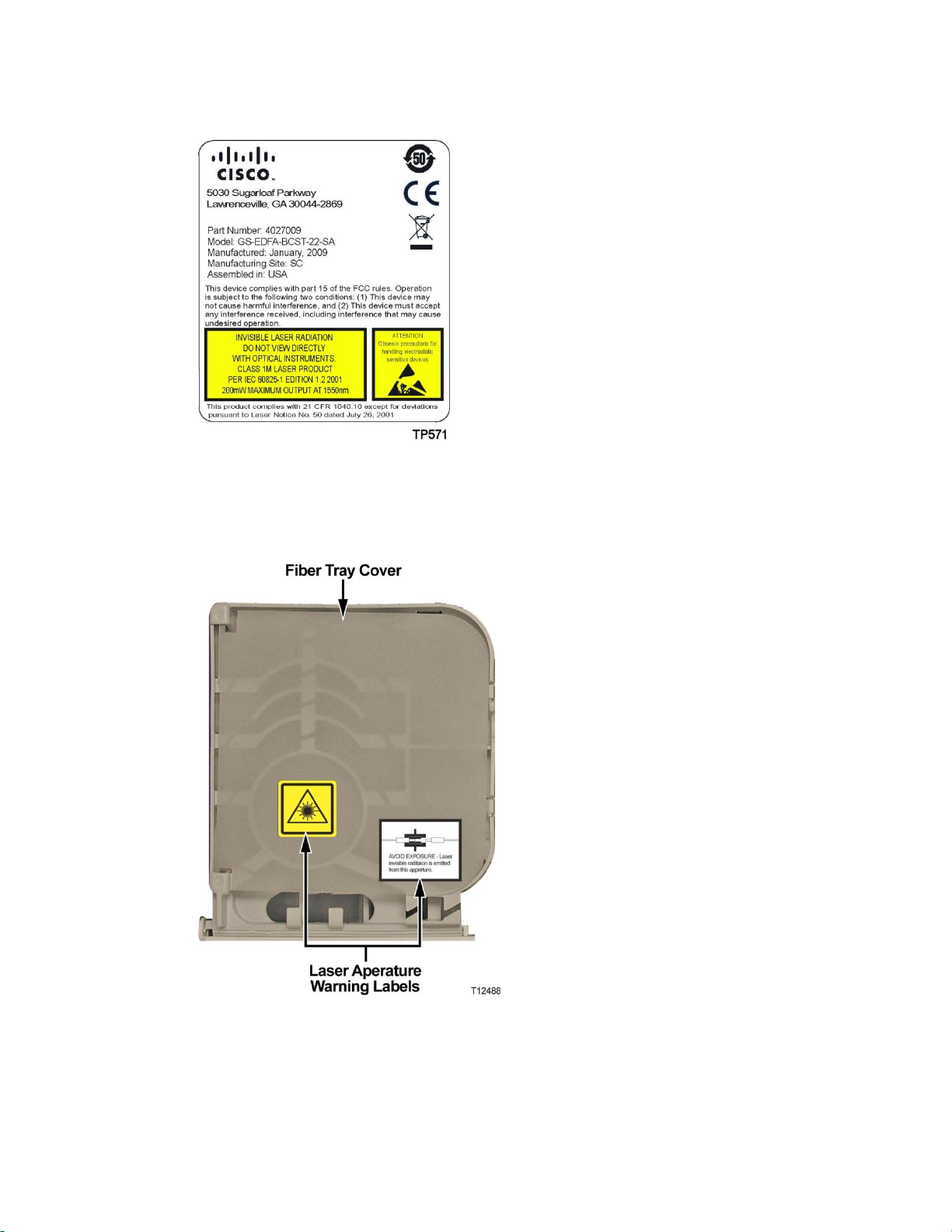
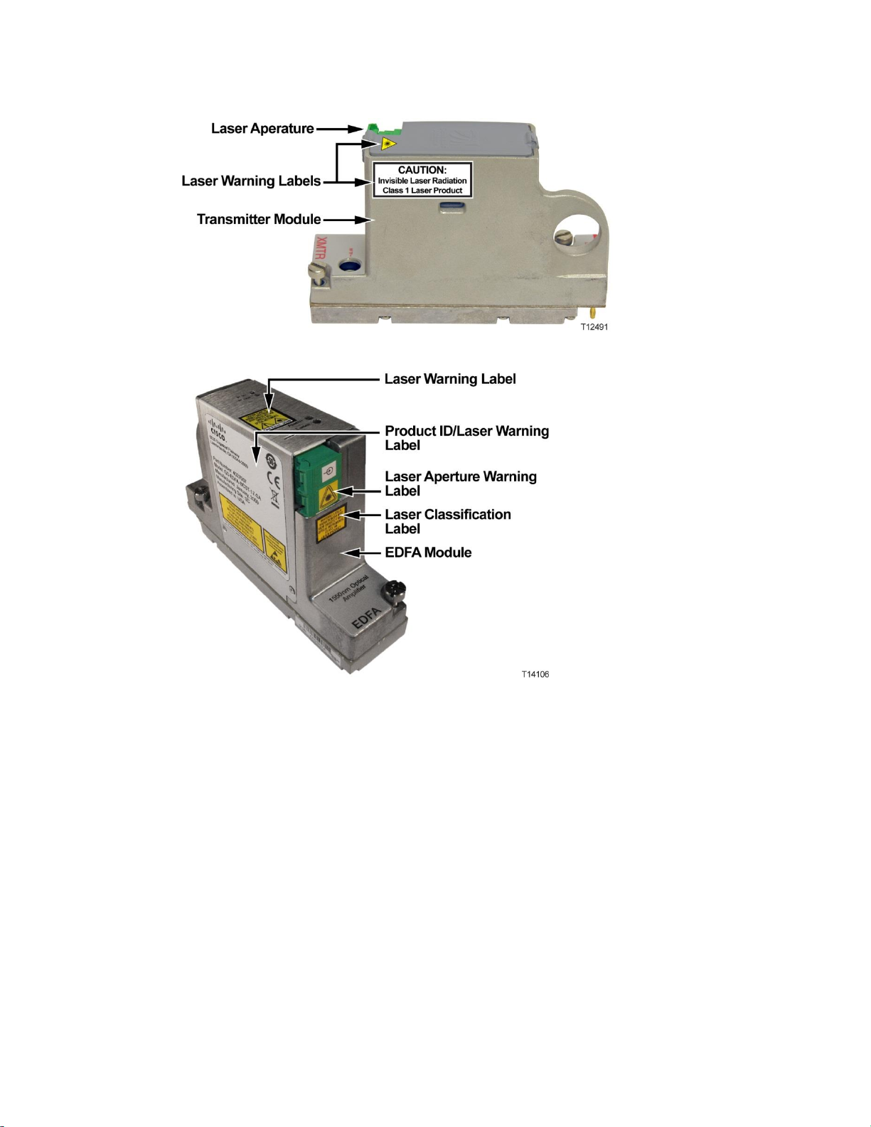
Location of Labels on Equipment

The following illustrations display the location of warning labels on this equipment.

Laser Warning Labels

xvii

Introduction

This manual describes the installation and operation of the 1.2 GHz GS7000 Node.

1 Chapter 1

General Information

In This Chapter

 Equipment Description .......................................................................... 2

Chapter 1 General Information

Equipment Description

Overview

This section contains a physical and functional description of the 1.2 GHz GS7000 Node.

Physical Description

The 1.2 GHz GS7000 Node is the latest generation 1.2 GHz optical node platform which uses the housing developed for the GS7000 Node Platform, but it has been painted for improved thermal performance. The housing has a hinged lid to allow access to the internal electrical and optical components. The housing also has provisions for strand, pedestal, or wall mounting.

Note: The 1.2 GHz GS7000 node is painted white, and the pictures in this document which use unpainted housings are used as references.

The base of the housing contains:

 an RF amplifier module  AC power routing  forward and reverse configuration modules (configuration will vary)

The lid of the housing contains:

 a fiber management tray and track (included in all nodes)  optical receiver and transmitter modules (configuration will vary)  EDFA (erbium-doped fiber amplifier) modules and optical switch modules

(for hub node application)

 power supplies (one or two)  a status monitor/local control module (optional)

Not every 1.2 GHz GS7000 Node contains all of these modules. The 1.2 GHz GS7000 Node is a versatile node that can be configured to meet various network requirements.

Equipment Description

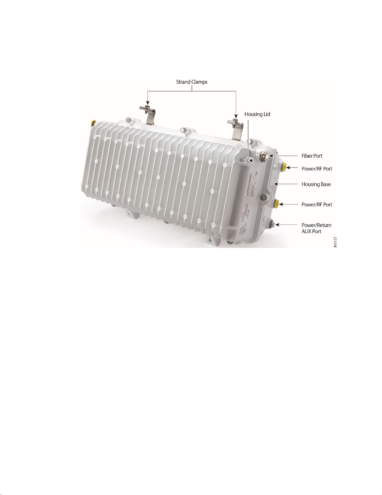
The following illustration shows the external housing of the 1.2 GHz GS7000 Node.

Chapter 1 General Information

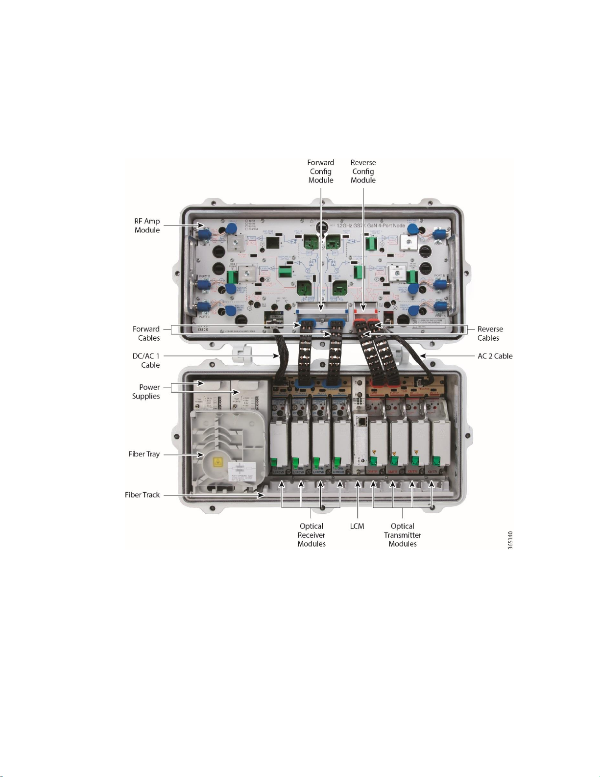
The following illustration shows the 1.2 GHz GS7000 Node internal modules and components.

Functional Description

Node

The 1.2 GHz GS7000 Node is used in broadband hybrid fiber/coax (HFC) networks. It is configured with the receivers, transmitters, configuration modules, and other modules to meet your unique network requirements. This platform allows independent segmentation and redundancy for both the forward and reverse paths in a reliable, cost-effective package.

Equipment Description

The 1.2 GHz GS7000 Node receives forward optical inputs, converts the input to an electrical radio frequency (RF) signal, and outputs the RF signals at up to six ports. The forward bandwidth is from 54 MHz (or 86, 102, 258 MHz) to 1218 MHz. The lower edge of the passband is primarily determined by the diplex filter and the reverse amplifier assembly. Diplex filter choices are 54 MHz, 86 MHz, 102 MHz, and 258 MHz.

The forward path of the 1.2 GHz GS7000 Node can be deployed with a broadcast 1310/1550 nm optical receiver with common services distributed to either four output ports (all high level) or six output ports (two high level and four lower level). The forward path can also be segmented by using one optical receiver that feeds all output ports, two independent optical receivers that each feed half of the node’s output ports (left/right segmentation) or four independent optical receivers that feed four independent forward paths. Forward optical path redundancy is supported via the use of optional local control module. The type of forward segmentation and/or redundancy is determined by the type of RF amplifier assembly and Forward Configuration Module installed in the node.

The 1.2 GHz GS7000 Node’s reverse path is equally flexible. Reverse traffic can be segmented or combined and routed to up to four DFB reverse optical transmitters, or up to four Enhanced Digital Return reverse optical transmitters as part of our EDR system. Redundant (back-up) transmitters may be utilized. In addition, an auxiliary input path is provided for reverse signal injection (5 - 210 MHz). Reverse segmentation and/or redundancy are determined by the type of Reverse Configuration Module installed in the node.

The 1.2 GHz GS7000 Node accepts Optical Transmitter Modules based on the existing 694x/GainMaker optical transmitters. Reverse optical transmitters can be installed to transmit data, video, or both. Reverse bandwidth is determined by the diplex filter and the reverse amplifier assembly. Diplex filter choices are 42/54 MHz, 65/86 MHz, 85/102 MHz, and 204/258 MHz.

The 1.2 GHz GS7000 Node utilizes the transmitter and receiver module covers that have been designed to allow fiber pigtails storage within them, providing improved fiber management within the node.

Up to four optical receivers and up to four analog or two digital transmitters can be installed in the 1.2 GHz GS7000 Node.

45 - 90 V AC input power is converted to +24.5, +8.5, -6.0, and +5.5 V DC by an internal power supply to power the 1.2 GHz GS7000 Node.

Hub Node

The GS7000 Hub Node performs the same functions as the GS7000 Node with the added benefit of also providing optical gain and optical switching capability. The hub node allows you to push fiber deeper into your network while taking advantage

Chapter 1 General Information

of the RF plant that is already in place.

The GS7000 Node can be upgraded to a GS7000 Hub Node in the field. This is accomplished by the installation of optical amplification (EDFA) modules, optical switching modules, and the Status Monitor/Local Control Module in the node lid. The GS7000 Hub Node can then serve as a traditional node feeding the local HFC plant and as an optical hub with the optical amplifiers. The node hub with the amplifiers can service up to 32 nodes at a distance of 50 km with only three fibers.

EDFAs are available in 17 dBm, 20 dBm, and 22 dBm for broadcast constant output power. A 17 dBm, 20 dBm and 21 dBm narrowcast constant gain EDFA version is available to fit any architecture for requirements like DWDM narrowcasting.

The optical switch module is used for switching the input of an EDFA module from a primary signal to a backup or secondary signal. The switch is monitored and controlled by the Status Monitor/Local Control Module (SM/LCM) in the node.

A specific model of the SM/LCM is required for use in the hub node. This SM/LCM model monitors and controls several EDFA and optical switch parameters and functions while continuing to monitor the standard node components.

Features

The 1.2 GHz GS7000 Node has the following features:

 Six port 1.2 GHz RF platform  Uses rugged GaN Technology on the output stage  Uses standard GainMaker style accessories (i.e., attenuator pads, equalizers,

diplexers and crowbar)

 Field accessible plug-in Forward Interstage Linear Equalizers,

Forward/Reverse Configuration Modules, and Node Signal Directors

 3-state reverse switch (on/off/-6 dB) allows each reverse input to be isolated

for noise and ingress troubleshooting (status monitor or local control module required)

 Auxiliary reverse injection (5 - 210 MHz) configurable on up to 2 ports (port 3

or port 6)

 Positions for up to 4 optical receivers and 4 optical transmitters in housing lid  Provides hub node functionality with addition of available optical amplifier

and optical switch modules

 Optional low-cost Local Control Module may be installed in conjunction with

a Redundant Forward Configuration Module to allow optical forward path

Equipment Description

redundancy when no status monitor is present

 Fiber entry ports on both ends of housing lid  Fiber management tray and track provides easy access to fiber connections  Primary and redundant power supplies with passive load sharing  Spring loaded seizure assemblies allow coax connectors to be installed or

removed without removing amplifier chassis or spring loaded mechanism from the rear of the housing base

 Dual/Split AC powering  Space provided for mounting WDM modules inside the housing lid.

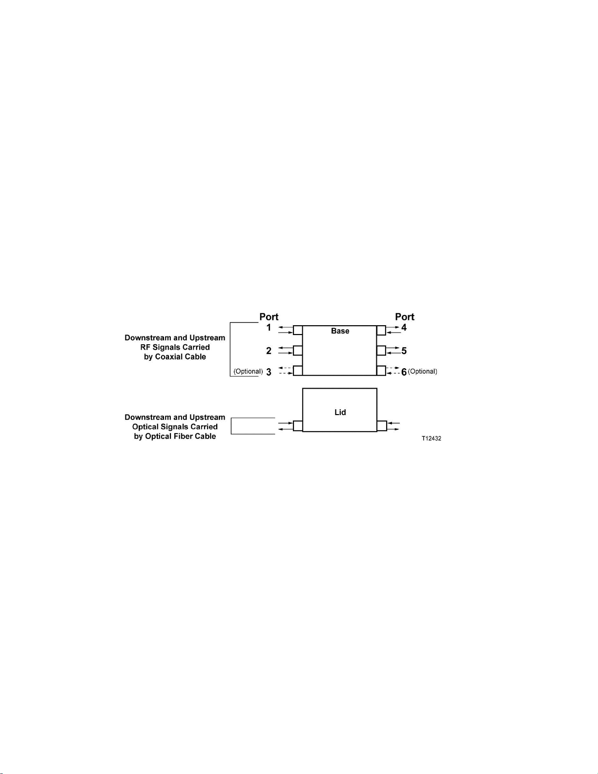
Node Inputs/Outputs Diagram

The following diagram shows the system-level inputs and outputs of the 1.2 GHz GS7000 Node.

 The AC can be applied to any RF port and routed, if required, to the other

ports.

 The DC power supply modules can be fed by any RF port (1 through 6).

Modules Functional Descriptions

This table briefly describes each module. The 1.2 GHz GS7000 Node may not contain all these modules. See Theory of Operation (on page 15) for detailed descriptions of the modules.

Chapter 1 General Information

Module

Description

RF Amplifier

The RF Amplifier Module includes:



four separate and independent forward amplification paths, each having one or two RF outputs.



four independent reverse inputs.



forward and reverse bandwidths that are established by diplexer and reverse amplifier assembly selection.

Forward Configuration

There are several types of this module.

The 1x4 Forward Configuration Module (FCM) is used when the 1.2 GHz GS7000 Node is configured with a single optical receiver routed to all four outputs of the amplifiers. This module splits the signals equally to the inputs of the RF amplifier module. The 1x4 Forward Configuration Modules with forward RF injection are similar to the 1x4 Forward Configuration Modules, but are used with the Forward Local Injection (FLI) Module. The FLI Module routes an RF signal from an external source to the Forward Configuration Module which is then coupled with other inputs from an optical receiver.

The 1x4 Redundant Forward Configuration Module is used when the

1.2 GHz GS7000 Node is configured with two optical receivers routed to all four outputs of the amplifiers in a redundant configuration. Receiver 1 is the primary receiver and Receiver 2 is the backup. The active receiver is selected with a status monitor or local control monitor.

Equipment Description

Module

Description

Forward Configuration (cont'd)

The 1x4 Redundant Forward Configuration Modules with forward RF injection are similar to the 1x4 Redundant Forward Configuration Modules, but are used with the Forward Local Injection (FLI) Module. The FLI Module routes an RF signal from an external source to the Forward Configuration Module which is then coupled with other inputs from an optical receiver.

The 2x4 Forward Configuration Module is used when the 1.2 GHz GS7000 Node is configured with two optical receivers, each feeding two/three outputs of the amplifier module. In this configuration, the node serving area is divided in half in the forward direction. Receiver 1 is routed to RF amplifier Ports 4 and 5/6, while Receiver 3 is routed to RF amplifier Ports 1 and 2/3.

The 2x4 Redundant Forward Configuration Module is used when the GS7000 Node is configured with four optical receivers with each pair feeding two/three RF outputs of the amplifier module in a redundant configuration. In this configuration, the node serving area is divided in half, with redundancy, in the forward direction. Receivers 1 (primary) and 2 (redundant) are routed to RF amplifier Ports 4 and 5/6, while Receivers 3 (primary) and 4 (redundant) are routed to RF amplifier Ports 1 and 2/3. The active receiver is selected with a status monitor or local control monitor.

The 3x4 Forward Configuration Module is used when the 1.2 GHz GS7000 Node is configured with three receivers each feeding one/two/three/four outputs of the amplifier module. Two versions of this module are available. In one version Receiver 1 is routed to RF amplifier ports 4/5/6, Receiver 3 is routed to port 1, and Receiver 4 is routed to ports 2/3. In the other version Receiver 1 is routed to RF amplifier ports 5/6, Receiver 2 is routed to port 4, and Receiver 4 is routed to ports 1/2/3. (Note that the 3x4 FCM can only be used with the 4-way RF amplifier module.)

The 4x4 Forward Configuration Module is used when the 1.2 GHz GS7000 Node is configured with four optical receivers with each feeding separate RF outputs of the amplifier module. Receiver 1 is routed to RF amplifier Ports 5/6. Receiver 2 is routed to RF amplifier Port 4. Receiver 3 is routed to RF amplifier Port 1. Receiver 4 is routed to RF amplifier Ports 2/3. (Note that the 4x4 FCM can only be used with the 4-way RF amplifier module.)

Chapter 1 General Information

Module

Description

Reverse Configuration

There are several types of this module.

The 4x1 Reverse Configuration Module (RCM) with auxiliary reverse RF injection combines all four reverse RF inputs (Ports 1, 2/3,

4, and 5/6) of the node and routes the signal to Transmitter 1. An RF signal from an external source can optionally be injected and coupled with the reverse RF inputs on Ports 3/6 and routed to Transmitter 1.

The 4x1 Redundant Reverse Configuration Module combines all four reverse RF signals (Ports 1, 2/3, 4 and 5/6) together, splits this RF signal and routes it to Transmitters 1 and 2.

The 4x2 Reverse Configuration Module with auxiliary reverse RF injection combines reverse inputs from Ports 1 and 2/3 and routes

them to Transmitter 1; it also combines reverse inputs from Ports 4 and 5/6 and routes them to Transmitter 3. An RF signal from an external source can optionally be injected and coupled with reverse RF inputs from Ports 3/6 and routed to Transmitter 1.

The 4x2 Redundant Reverse Configuration Module combines reverse inputs from Ports 1 and 2/3 and routes them to Transmitters 1 and 2; it also combines reverse inputs from Ports 4 and 5/6 and routes them to Transmitters 3 and 4.

The 4x3 Reverse Configuration Module with auxiliary reverse RF injection is available in two types. The

left-combined/right-segmented version combines reverse inputs from Ports 1 and 2/3 and routes them to Transmitter 1; it also routes reverse inputs from Port 4 to Transmitter 3 and from Ports 5/6 to Transmitter

4. An RF signal from an external source can optionally be injected at Ports 3/6 and coupled with the reverse RF input from Port 1 and routed to Transmitter 1. The left-segmented/right-combined version combines reverse inputs from Ports 4 and 5/6 and routes them to Transmitter 4; it also routes reverse inputs from Port 1 to Transmitter 1 and from Ports 2/3 to Transmitter 2. An RF signal from an external source can optionally be injected at Ports 3/6 and coupled with the reverse RF inputs from Ports 2/3 and 1 and routed to Transmitter 1.

Equipment Description

Module

Description

Reverse Configuration (cont'd)

The 4x4 Reverse Configuration Module with auxiliary reverse RF injection routes reverse inputs from Port 1 to Transmitter 1, from Port

2/3 to Transmitter 2, from Port 4 to Transmitter 3, and from Port 5/6 to Transmitter 4. An RF signal from an external source can optionally be injected and coupled with reverse RF inputs from Ports 3/6 and routed to Transmitter 1. (Note that this module is typically installed when using EDR multiplexing digital reverse modules. Since the digital reverse module occupies the physical space that transmitters 3 and 4 normally occupy in the node base, this reverse configuration module is typically used with a 6-port optical interface board.)

Optical Receiver

This module converts an optical signal from the headend into a forward path RF signal. An SC/APC fiber connector is standard. Optical power, test points, and status LEDs are provided.

Optical Transmitter

This module converts reverse path RF signals from the network into an optical signal. An SC/APC fiber connector is standard. Multiple transmitter options are available such as uncooled DFB, 1550 ITU, and EDR. EDR uses the included LC/APC connector that jumps over to an SC/APC bulkhead. Optical power, test points, and status LEDs are provided.

Optical Amplifier (EDFA)

Erbium-doped fiber amplifier modules are available in two categories: broadcast and narrowcast (gain-flattened). EDFAs are available in 17 dBm, 20 dBm, and 22 dBm for broadcast constant output power. A 17 dBm, 20 dBm and 21 dBm narrowcast constant gain EDFA version is available to fit any architecture for requirements like DWDM narrowcasting. EDFA modules are single-wide, single-output devices. The modules mount in receiver or transmitter slots on the optical interface board in the node lid using a reversible pin adapter. The EDFA is monitored and controlled by the Status Monitor/Local Control Module in the node.

Optical Switch

The optical switch module is used for switching the input of an EDFA module from a primary signal to a backup or secondary signal. The module mounts in receiver or transmitter slots on the optical interface board in the node lid using a reversible pin adapter. The switch is monitored and controlled by the Status Monitor/Local Control Module in the node.

Chapter 1 General Information

Module

Description

Status Monitor/ Local Control Module

(SM/LCM)

The local control module monitors the input optical power of up to four receivers and four transmitters, plus AC power entry and power supply voltage rails. It also provides local reverse path wink and shutdown capabilities through the PC-based GS7000 ViewPort software. It can be upgraded to a status monitor which provides node monitoring and control capability at the cable plant's headend. This module is not required for normal operation of the node. In a hub node application the SM/LCM also monitors and controls the operation of the EDFAs and optical switches.

Power Supply

The 1.2 GHz GS7000 power supply module has multiple output voltages of +24.5, +8.5, -6.0, and +5.5 V DC. A second power supply can be installed in the node for redundancy or load sharing.

The 1.2 GHz GS7000 Node can be set up in the following powering configurations:



two power supplies powered by different AC sources



two power supplies using the same AC source



a single supply using a single AC source

Fiber Management Tray and Track

The fiber management system secures and protects the optical fiber inside the node housing.

Optical Interface Board

The Optical Interface Board (OIB) provides all interconnections between the modules in the housing lid of the 1.2 GHz GS7000 Node. Each module in the lid plugs directly into the OIB through a connector header or row of sockets. Input attenuator pads are provided on the OIB for each optical receiver in the housing lid. Output attenuator pads are provided on the OIB for each optical transmitter in the housing lid.

Equipment Description

Ordering Information

The 1.2 GHz GS7000 Node is available in a wide variety of configurations. Please refer to the 1.2 GHz GS7000 Node Data Sheet for a full listing of the configured node, components, and accessories that are available.

Note: Please consult with your Account Representative, Customer Service Representative, or System Engineer to determine the best configuration PID for your particular application.

Note: Please consult with your Account Re presentative, Customer Service Representative, or System Engineer to determi ne the best configuration for your particular application.

Introduction

This chapter describes the theory of operation for the 1.2 GHz GS7000 Node, including functional descriptions of each module in the node.

The 1.2 GHz GS7000 Node is comprised of two parts, the lid and the base.

The lid houses an optical interface board (OIB), and some of the following products: one to four optical receivers, one to four optical transmitters, one digital return module with one or two digital transmitters, EDFA (optional), optical switch (optional), a status monitor (optional) or a local control module (optional), one or two power supplies, and a fiber management tray/track.

The base houses the RF amplifier module and the accessories that plug into it. These accessories include a forward configuration module, four forward band linear equalizer modules, multiple attenuator pads, two node signal director jumper or splitter modules, and two auxiliary reverse injection director modules. Also contained within the launch amplifier module are a reverse auxiliary jumper/combiner/amplifier/termination module and a reverse configuration module.

2 Chapter 2

Theory of Operation

Chapter 2 Theory of Operation

In This Chapter

 System Diagrams .................................................................................. 17

 Forward Path ......................................................................................... 21

 Reverse Path .......................................................................................... 22

 Power Distribution ............................................................................... 23

 RF Amplifier Module ........................................................................... 24

 Forward Configuration Module ......................................................... 29

 Reverse Configuration Module .......................................................... 34

 Optical Interface Board (OIB) .............................................................. 38

 Optical Receiver Module ..................................................................... 39

 Optical Analog Transmitter Modules ................................................ 43

 Optical Amplifier (EDFA) Modules ................................................... 45

 Optical Switch Module ........................................................................ 52

 Local Control Module .......................................................................... 58

 Power Supply Module ......................................................................... 61

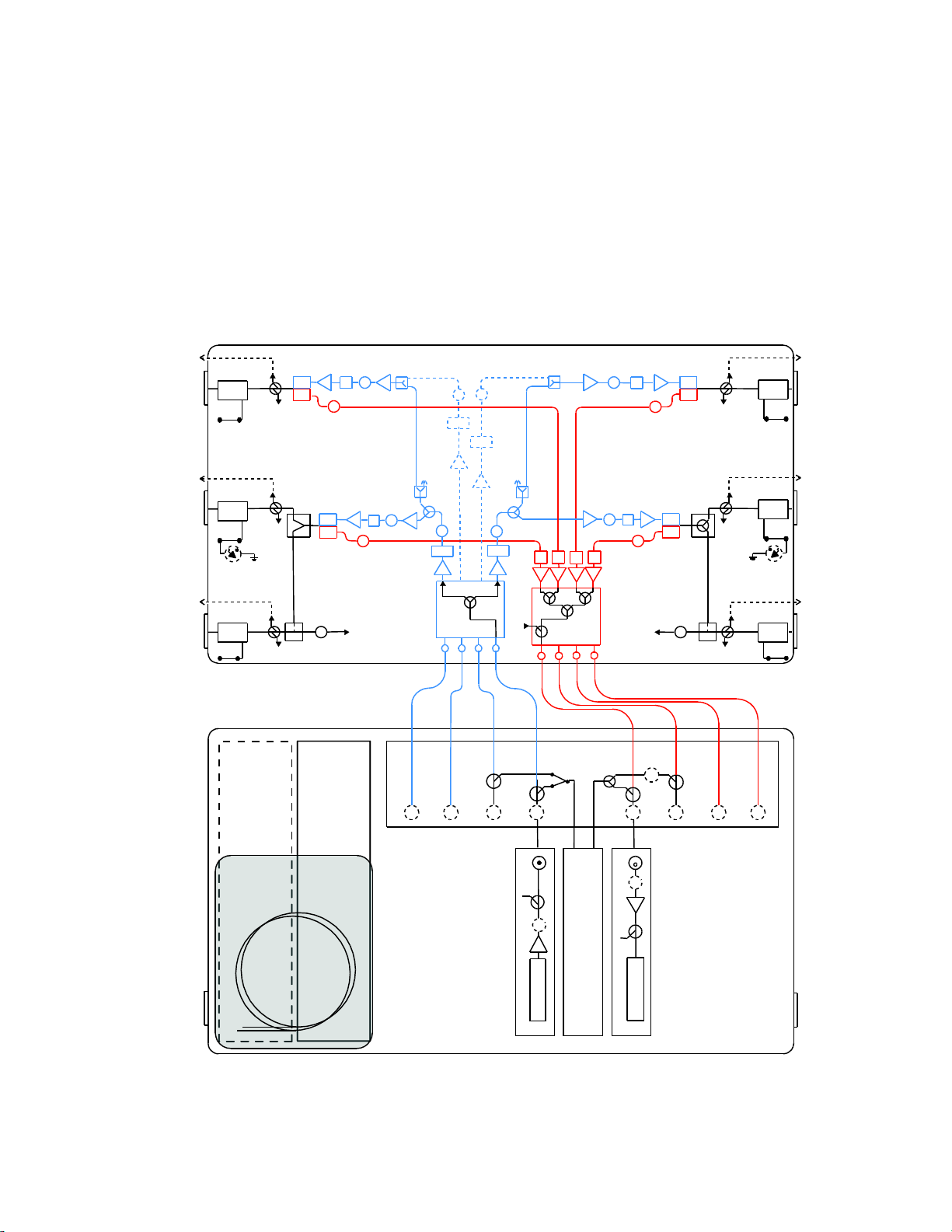
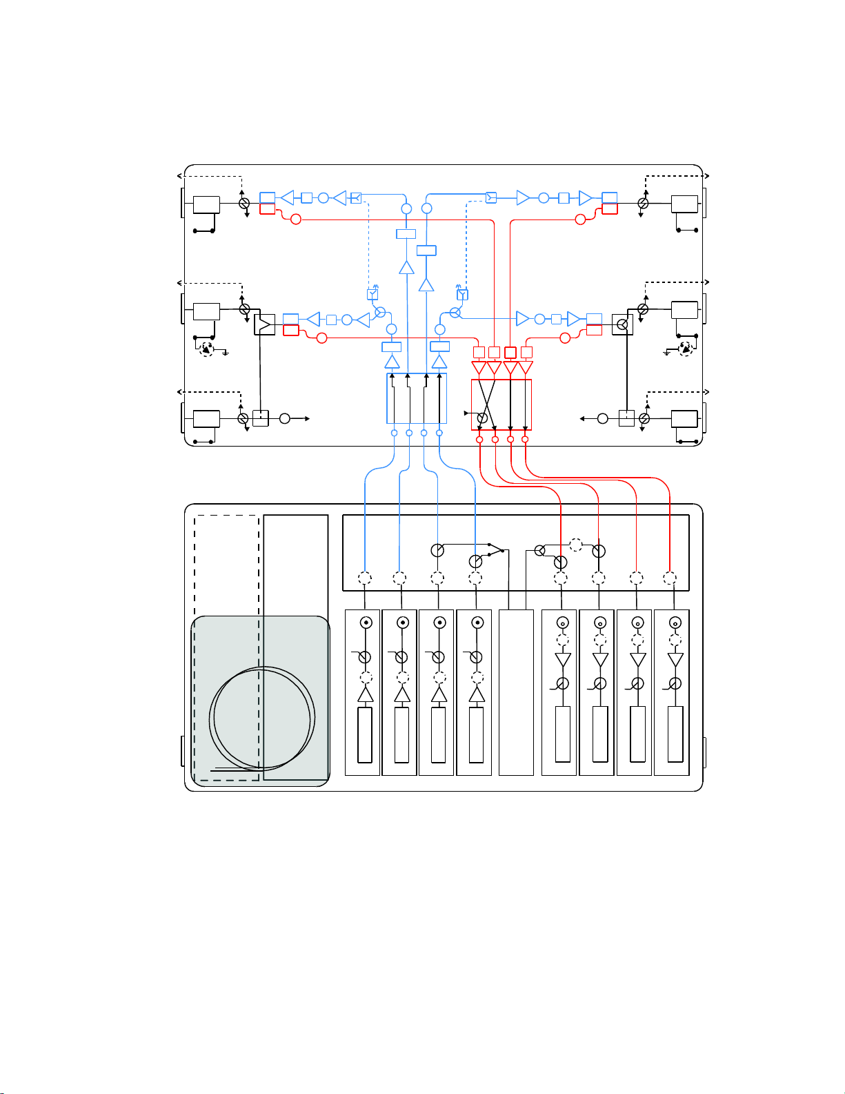
System Diagrams

F2F1

Optical

Interface Board

Power

Supply #1

Power Dire ctor

FWD

REV

FWD

REV

Aux. Rever se Injection

Director

Node

Signal Dir ector

Jumper

Pad

Crowbar

Power Dire ctor

FWD

REV

FWD

REV

(to RCM)

-210 MHz

Reverse In jection

Option

Aux. Rever se Injection

Director

Aux. Rev

Injection

Node

Signal Dir ector

Splitter

Pad

Crowbar

Power Dire ctor

Byp ass

RS = rever se switch

1x4

Forward Configuration

Module

4x1 Reverse

Configuration Module

w/Aux Reverse

RF Injection

Fiber Tray

Power

Supply #2

RCVR

# 1

XMT R # 1

Pad

Pad Pad Pad Pad PadPadPad

Pad

-20 dB

Rev. TP

-20 dB Rev. TP

-20 dB

Rev. TP

-20 dB Rev. TP

-20 dB

Rev. TP

-20 dB

Rev. TP

Thermal

PadPad

Thermal

Pad

Thermal

RF Switch

(to RCM)

-210 MHz

Reverse In jection

Option

External

-20 dB TP

-20 dB Fwd. TP

External

-20 dB TP

-20 dB

Fwd. TP

Power Dire ctor

-20 d

Fwd. TP

-20 d

Fwd. TP

-20 d

Fwd. TP

External

-20 dB TP

External

-20 dB TP

External

-20 dB TP

External

-20 dB TP

-20 dB

Fwd. TP

Byp ass

RS RS

Functional Diagrams: 4-Way Forward Segmentable Node

The following diagrams show the signal flow through the 4-way forward segmentable node.

Non-Segmented

Chapter 2 Theory of Operation

Left-Right Segmented

System Diagrams

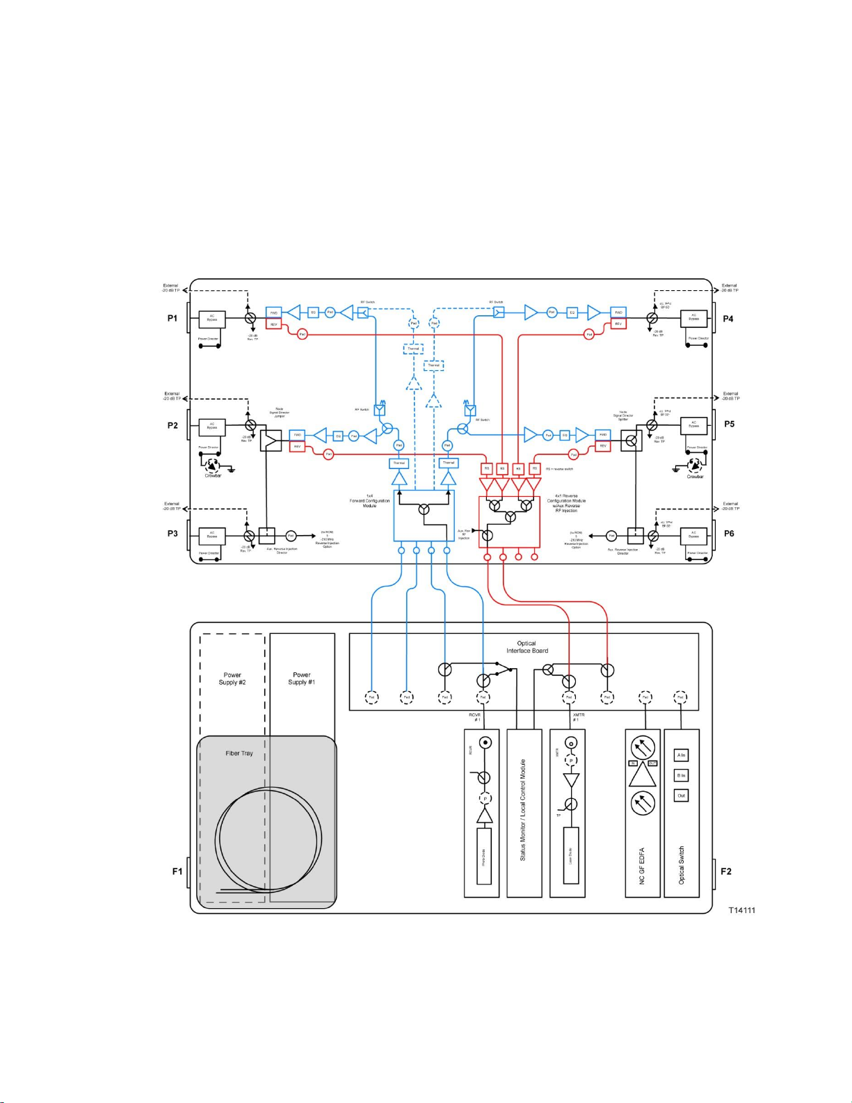
Fully Segmented

F2F1

Optical

Interface Board

Power

Supply #1

Power Dire ctor

FWD

REV

FWD

REV

Aux. Rever se Injection

Director

Node

Signal Dir ector

Jumper

Pad

Crowbar

Power Dire ctor

FWD

REV

FWD

REV

(to RCM)

-210 MHz

Reverse In jection

Option

Aux. Rever se Injection

Director

Aux. Rev

Injection

Node

Signal Dir ector

Splitter

Pad

Crowbar

Power Dire ctor

Byp ass

RS = rever se switch

4x4

Forward Configuration

Module

4x4 Reverse

Configuration Module

w/Aux Reverse

RF Injection

Fiber Tray

Power

Supply #2

RCVR

# 1

RCVR

# 2

RCVR

# 3

RCVR

# 4

XMT R # 1

XMT R # 2

XMT R # 3

XMT R # 4

Pad

Pad Pad Pad Pad PadPadPad

Pad

-20 dB Rev. TP

-20 dB

Rev. TP

-20 dB

Rev. TP

-20 dB

Rev. TP

-20 dB Rev. TP

-20 dB

Rev. TP

Thermal

PadPad

Thermal

Pad

Thermal

RF Switch

(to RCM)

-210 MHz

Reverse In jection

Option

External

-20 dB TP

-20 dB Fwd. TP

External

-20 dB TP

-20 dB Fwd. TP

Power Dire ctor Power Dire ctor

-20 d

Fwd. TP

-20 d

Fwd. TP

-20 d

Fwd. TP

External

-20 dB TP

External

-20 dB TP

External

-20 dB TP

External

-20 dB TP

-20 dB Fwd. TP

Byp ass

RS RS

Chapter 2 Theory of Operation

Functional Diagram: Hub Node

The following diagram shows the signal flow through a 4-way non-segmented hub node.

Forward Path

Stage

Description

1310 nm or 1550 nm optical signals from the headend are applied to receiver module 1 (and/or modules 2, 3, and 4, if used) in the 1.2 GHz GS7000 Node.

The receiver module detects the signal on the optical carrier applied to it and outputs an electrical RF signal to the node Optical Interface Board (OIB).

The RF signals travel across the OIB and cables to the Forward Configuration Module (FCM). The FCM determines how RF signals from the different receiver modules are routed to the four independent forward amplification paths in the RF amplifier module. The 1X4 FCM splits the RF signals entering it equally between the four forward amplification paths in the RF amplifier module.

Each of the forward amplification paths in the RF amplifier module is composed of one input amplification stage and one interstage amplification stages in series followed by a power doubler output amplification stage. This topology provides one driven output port for each of the forward amplification paths in the RF amplifier module, for a total of four driven node output ports.

Each of the forward amplification paths in the RF amplifier module also contains padding, trimming, thermal compensation, equalization, and filtering circuitry.

Node signal directors are present at two of the nodes forward output ports and allow the signals at those ports to be redirected to the nodes auxiliary output ports or split equally between the primary and auxiliary node output ports. In this way, the node can be configured to have up to six output ports.

Introduction

Forward path refers to signals received by the node from the headend. These signals are amplified in the node and routed to subscribers through the cable distribution network.

4-Way Forward Path Signal Routing

1.2 GHz GS7000 Node 4-way forward path signal routing functions are described below.

Chapter 2 Theory of Operation

Reverse Path

Stage

Description

Reverse path RF signals are applied to node output ports 1, 2, 4, and 5. A fifth reverse path RF signal can be applied to node auxiliary output port 3 or 6 if the node is configured for local reverse path injection.

The RF signals from each of the four node output ports are amplified independently in the RF amplifier module and routed to the Reverse Configuration Module (RCM).

Each of the reverse amplification paths in the RF amplifier module also contains padding, trimming, filtering, -6 db wink, and RF On/Off switch circuitry.

The RCM determines how RF signals from the different node output ports are combined and routed to the four transmitter module paths on the Optical Interface Board (OIB). The 4X1 RCM combines the reverse path signals from the four node output ports together and directs them to the transmitter module 1 path on the OIB. (Note that other RCMs combine and direct signals to OIB transmitter module paths 2, 3, and 4 differently.)

The RF signals travel across the OIB to transmitter module 1 (and/or modules 2, 3, and 4, if used and proper RCM is installed.) The transmitter modulates the RF signals entering it onto an optical carrier and routes it through the fiber portion of the network back to the headend.

Introduction

Reverse path refers to signals received by the node from the cable distribution network. These signals are amplified in the node and returned to the headend optically through the fiber portion of the network. The reverse path is not used in all networks.

Reverse Path Signal Routing

1.2 GHz GS7000 Node reverse path signal routing functions are described below.

Note: Node output ports 3 and 6 can be configured as primary reverse ports. See Reconfiguring Reverse Signal Routing (on page 113) for further details on this configuration.

Power Distribution

Stage

Description

45 to 90 V AC is applied to one or two power supply modules in the 1.2 GHz GS7000 Node.

The power supply module(s) convert(s) the AC input to +24.5, +8.5, -6.0, and +5.5 V DC.

The +24.5, +8.5, -6.0, and +5.5 V DC lines are routed to 1.2 GHz GS7000 Node internal modules.

If two power supplies are installed and both are active, the load is shared equally between them.

An AC segmentable shunt is available to separate the AC connection to ports 1-3 from that of ports 4-6. This allows the node to be configured where one power supply is powered from ports 1-3 and a second power supply is powered from ports 4-6.

Introduction

The 1.2 GHz GS7000 Node is powered by one or two power supplies.

Power Distribution

1.2 GHz GS7000 Node power distribution functions are described below.

Chapter 2 Theory of Operation

RF Amplifier Module

Port 3

Port 2

Port 1

1.2GHz GS7000 Node

4 Way Forward Segmentable Launch Amplifier Module

Digital

Control

Pre

Amp

Forward Configuration

Module

Forward Input

R1R2R4

Digital Control

Pre

Amp

AC 2

Power

Surge

Protection

Rev. TP

Fwd. TP

Rev. TP

Fwd. TP

Port 6

Rev. TP

Port 5

Port 4

Output

GaN

Gain Block

Aux. Reverse

Injection

Director

Node Signal

Director

Splitter

Interstage

GaAs

Gain Block

Output

GaN

Gain Block

Tilt Pad EQ

Pad

EQPad

Pad

Ther

Interstage

GaAs

Gain Block

Switch

Pad

210 MHz Aux.

Reverse Injection

Option

Switch

Surge

Protection

AC 1

Power

Rev. TP

Fwd. TP

Rev. TP

Fwd. TP

Rev. TP

Aux. Reverse

Injection Director

Node Signal

Director

Jumper

Output

GaN

Gain Block

Pad

Pad B

Tilt

Pad

Ther

Pad

210 MHz Aux.

Reverse Injection

Option

Output

GaN

Gain Block

Pad

EQ PadPad

Ther

Switch

Interstage

GaAs

Gain Block

Switch

Pre

Amp

Interstage

GaAs

Gain Block

TrimTrim

Trim

Field Accessable

Plug-In

Factory Plug-In

Field Accessable

Split Upgrade

Low

High

Low

High

Low

High

Low

High

Low

High

Introduction

This section describes the RF amplifier module. The RF amplifier module contains the forward band and the reverse band amplifiers.

Functional Diagrams

The following diagrams show how the RF amplifier functions.

RF Amplifier Module

Reverse Amplifier PWB

Reverse Amplifier IC

with Integrated Attenuator

Digital Att

(Off - 0 - 6 dB)

Trim

Switch

Trim

Switch

Trim

Switch

Trim

Switch

Reverse Amplifier

Digital Control Circuitry

Digital Control

Parallel Output

Digital Control

Reverse

Aux. Jumper/ Comb./

Amp./ Term./

Module

LPF

Serial Input

. . .

Optical Interface PWB

Status Monitor or

Local Control Module

Receiver 1

Receiver 2

Receiver 3

Receiver 4

Power Supply 1

Power Supply 2

Pad

Switch

To Forward

Amplifier

Reverse

Config.

Module

Control

Digital Att

(Off - 0 - 6 dB)

Digital Att

(Off - 0 - 6 dB)

Digital Att

(Off - 0 - 6 dB)

Transmitter 4

Transmitter 3

Transmitter 2

Transmitter 1

Pad

Field Accessable

Plug-In

Field Accessable

Split Upgrade

Forward Band Amplification 4-Way Path Description

The RF amplifier module provides all forward signal amplification outside the optical receiver modules in the GS7000 Node.

The 4-way segmentable launch amplifier contains four independent forward amplification paths, each having one input near the center of the amplifier module and one, two or three outputs at one end of the amplifier module. Each of the forward paths is comprised of the forward configuration module, an input gain block, a frequency response trim circuit, a thermal compensation circuit, an inter-stage pad, a 2-way splitter or RF switch circuit, an inter-stage gain block, a plug-in forward band linear equalizer, an output pad, an output gain block, a diplex filter, a bi-directional 20 dB down forward test point, and finally an AC bypass circuit.

The thermal circuit on the RF amplifier module is designed to compensate for the RF forward path thermal movement of the entire node RF station. This includes the forward path amplifier module circuitry, RF cables, and optical interface board

Chapter 2 Theory of Operation

circuitry. It does not include the thermal movement of the optical receivers.

Forward Configuration Module

The forward configuration module determines the forward path topology in the RF amplifier module and the 1.2 GHz GS7000 Node. The output signals from one to four optical receivers enter the forward configuration module where they are combined and or directed to the two or four independent forward paths in the RF amplifier module. Forward path segmentation and/or redundancy are set by plugging the appropriate forward configuration module into the RF amplifier module. The forward configuration module is a plug-in, field accessible module. See Forward Configuration Module (on page 29) for more information.

Forward Band Linear Equalizer Module

The forward band linear equalizer module sets the overall forward path tilt of the RF amplifier module and the 1.2 GHz GS7000 Node. The 1.2GHz GS7000 Node launch amplifier is shipped with four 18.0 dB linear equalizers installed in the RF amplifier module. One equalizer is installed in each of the four amplifier module forward paths. This sets the nodes forward path tilt to 17.5 dB linear. Forward band linear equalizer modules of other values are available. This allows the nodes forward path tilt to be adjusted as needed. The forward band linear equalizer module is a plug-in, field accessible module. See the equalizer charts in Appendix A - Technical Information.

Node Signal Director Jumper/Splitter Module

The node signal director jumper/splitter module is a plug-in, field accessible module. It is present on the center output ports on either end of the RF amplifier module. The orientation of these modules determines where the RF amplifiers center output port signals are directed. The node signal director jumper allows the center output port signals to be routed to either the amplifiers primary center output port or to its auxiliary corner output port. The node signal director splitter module splits the center output port signals equally between the primary and auxiliary output ports.

Auxiliary Reverse Injection Director Module

The auxiliary reverse injection director module is a plug-in module. It is accessible only after the RF amplifier modules cover has been removed. Auxiliary reverse injection director modules are present on the auxiliary corner output ports on either end of the RF amplifier module. The orientation of these modules determine if the nodes auxiliary output ports are configured to be primary or split node output ports, or local reverse injection ports.

RF Amplifier Module

Reverse Band Amplification Path Description

The RF amplifier module provides all reverse signal amplification outside the optical transmitter modules in the 1.2 GHz GS7000 Node. It contains four independent reverse paths comprised of an AC bypass circuit, a bi-directional 20 dB down reverse test point, a diplex filter, an input pad, a low pass filter, a 6 dB switched attenuator, a 16 dB gain block, a second low pass filter, an RF on/off switch, a frequency response trim circuit, and a reverse configuration module. The 6 dB switched attenuator and RF on/off switch circuits allow each reverse path to have 6 dB (wink) and on/off capabilities. These circuits are controllable from the headend via the status monitor or locally via the local control module and a hand held controller. A serial communication link is provided between status monitor or local control module and the reverse band launch amplifier. Circuitry on the amplifier converts the serial communications to parallel control signals and routes them as needed.

The RF amplifier module also provides the routing for the auxiliary ports, 5 to 210 MHz reverse band local injection signals. Each of the two auxiliary port reverse band local injection paths is comprised of an AC bypass circuit, a bi-directional 20 dB down reverse test point, an input pad, and a reverse auxiliary jumper/amplifier/termination module. Signals from port 3 or port 6 of the nodes auxiliary path are directed by the reverse auxiliary/jumper/amplifier/termination module to the reverse configuration module.

Reverse Configuration Module

The reverse configuration module determines the reverse path topology in the RF amplifier module and 1.2 GHz GS7000 Node. The input signals from four independent amplifier module output ports and possibly the auxiliary reverse injection amplifier module port enter the reverse configuration module where they are combined and/or directed to one to four optical transmitters. Reverse path segmentation and or redundancy as well the ability to locally inject signals into the reverse path of the amplifier is set by plugging the appropriate reverse configuration module into the RF amplifier module. The reverse configuration module is a plug-in, field accessible module. See Reverse Configuration Module (on page 34) for more information.

Reverse Auxiliary Jumper/Combiner/Amplifier/Termination Module

The reverse auxiliary jumper/combiner/amplifier/termination module determines how reverse band signals, locally injected into the RF amplifier modules auxiliary ports, are routed within the amplifier module. The reverse auxiliary jumper module directs signals for one of the RF amplifiers auxiliary ports to the reverse configuration module.

The reverse auxiliary amplifier module amplifies signals for one or both of the RF

Chapter 2 Theory of Operation

amplifiers auxiliary ports and directs them to the reverse configuration module. The reverse auxiliary termination module terminates both auxiliary port reverse injection signal paths in 75 ohms as well as the path to the reverse configuration module.

Forward Configuration Module

Introduction

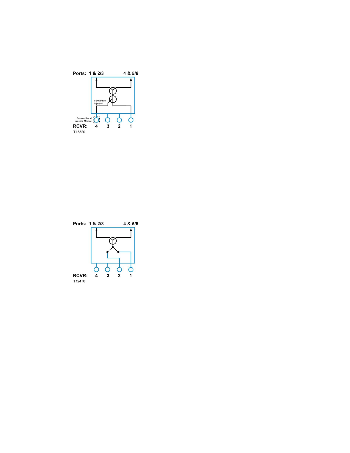
1x4 Forward Configuration Modules Description

The 1x4 Forward Configuration Module is used when the 1.2 GHz GS7000 Node is configured with a single optical receiver routed to all four outputs of the RF amplifier module. This module splits the signals equally to the inputs of the RF amplifier module.

The following diagram shows how this module functions.

1x4 Forward Configuration Modules with Forward RF Injection Description

The 1x4 Forward Configuration Modules with forward RF injection are similar to the 1x4 Forward Configuration Modules, but are used with the Forward Local Injection (FLI) Module. The FLI Module routes an RF signal from an external source to the Forward Configuration Module which is then coupled with other inputs from an optical receiver.

The following diagram shows how this module functions.

Chapter 2 Theory of Operation

1x4 Redundant Forward Configuration Modules Description

The 1x4 Redundant Forward Configuration Module is used when the 1.2 GHz GS7000 Node is configured with two optical receivers routed to all four outputs of the amplifiers in a redundant configuration. Receiver 1 is the primary receiver and Receiver 2 is the backup. The active receiver is selected with a digital signal from the status monitor/local control module.

The following diagram shows how this module functions.

1x4 Redundant Forward Configuration Modules with Forward RF Injection Description

The following diagram shows how this module functions.

Forward Configuration Module

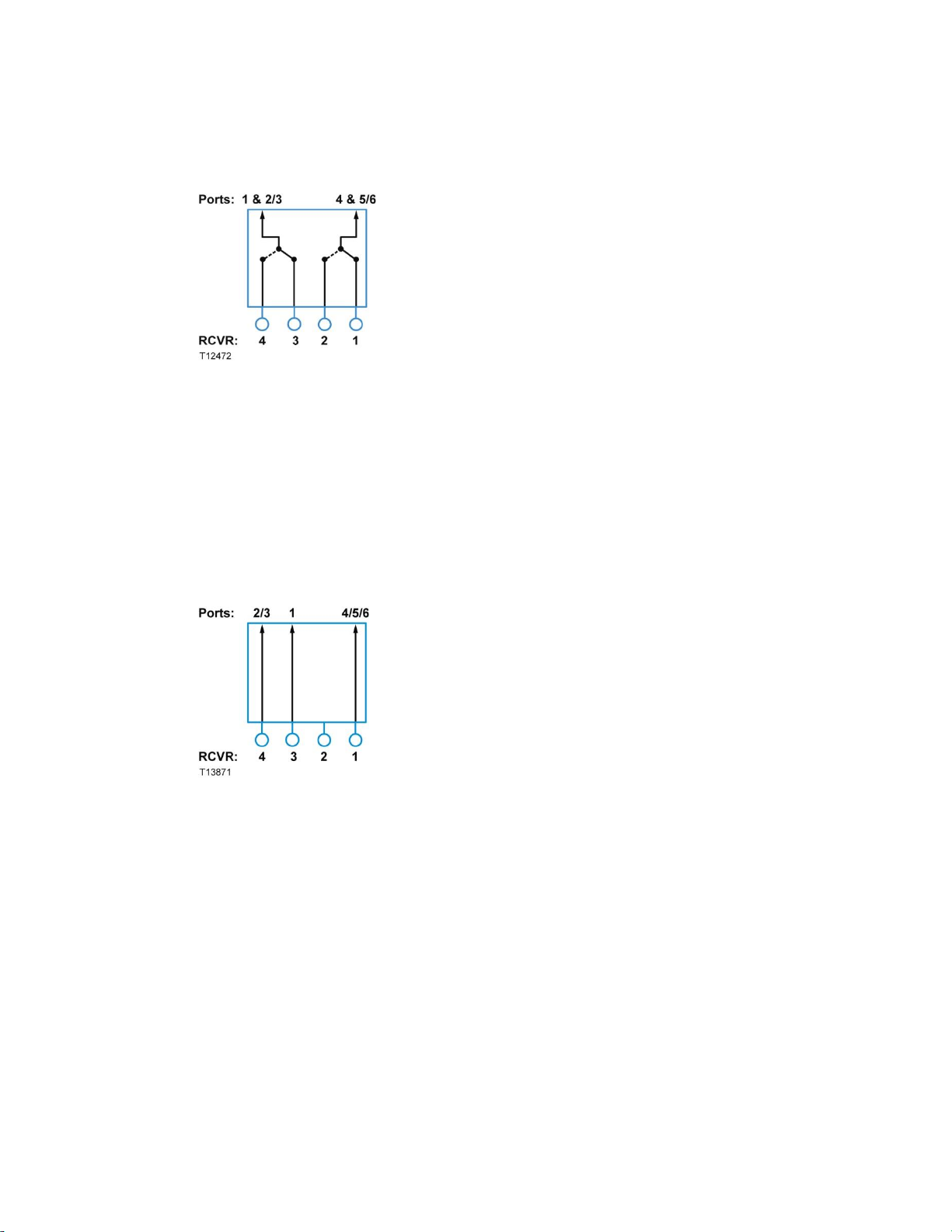
2x4 Forward Configuration Modules Description

The 2x4 Forward Configuration Module is used when the 1.2 GHz GS7000 Node is configured with two optical receivers, each feeding two outputs of the amplifier module. In this configuration, the node serving area is divided in half in the forward direction. Receiver 1 is routed to RF amplifier Ports 4 and 5/6, while Receiver 3 is routed to RF amplifier Ports 1 and 2/3.

The following diagram shows how this module functions.

2x4 Redundant Forward Configuration Modules Description

The 2x4 Redundant Forward Configuration Module is used when the 1.2 GHz GS7000 Node is configured with four optical receivers with each pair feeding two RF outputs of the amplifier module in a redundant configuration. In this configuration, the node serving area is divided in half for redundancy in the forward direction. Receivers 1 (primary) and 2 (redundant) are routed to RF amplifier Ports 4 and 5/6, while Receivers 3 (primary) and 4 (redundant) are routed to RF amplifier Ports 1 and 2/3. The active receiver is selected with digital signal from the status monitor/local control module.

The following diagram shows how this module functions.

Chapter 2 Theory of Operation

3x4-1, 3, 4 Forward Configuration Module Description

The 3x4-1, 3, 4 Forward Configuration Module is used when the 1.2 GHz GS7000 Node is configured with three receivers each feeding one/two/three/four outputs of the amplifier module. Receiver 1 is routed to RF amplifier ports 4/5/6, Receiver 3 is routed to port 1, and Receiver 4 is routed to ports 2/3.

Note: The 3x4-1, 3, 4 FCM can only be used with the 4-way RF amplifier module.

The following diagram shows how this module functions.

3x4-1, 2, 4 Forward Configuration Module Description

The 3x4-1, 2, 4 Forward Configuration Module is used when the 1.2 GHz GS7000 Node is configured with three receivers each feeding one/two/three/four outputs of the amplifier module. Receiver 1 is routed to RF amplifier ports 5/6, Receiver 2 is routed to port 4, and Receiver 4 is routed to ports 1/2/3.

Note: The 3x4-1, 2, 4 FCM can only be used with the 4-way RF amplifier module.

The following diagram shows how this module functions.

Forward Configuration Module

4x4 Forward Configuration Module Description

Note: The 4x4 FCM can only be used with the 4-way RF amplifier module.

The following diagram shows how this module functions.

Chapter 2 Theory of Operation

Reverse Configuration Module

Introduction

The reverse configuration module determines the reverse path topology in the RF amplifier module and 1.2 GHz GS7000 Node. The input signals from four independent amplifier module output ports enter the reverse configuration module where they are combined and/or directed to one to four optical transmitters. The various types of the reverse configuration module are described below.

4x1 Reverse Configuration Module with Auxiliary Reverse RF Injection Description

The 4x1 Reverse Configuration Module with auxiliary reverse RF injection combines all four reverse RF inputs (Ports 1, 2/3, 4, and 5/6) of the node and routes the signal to Transmitter 1. An RF signal from an external source can optionally be injected and coupled with the reverse RF inputs on Ports 3/6 and routed to Transmitter 1.

The following diagram shows how this module functions.

4x1 Redundant Reverse Configuration Module Description

The 4x1 Redundant Reverse Configuration Module combines all four reverse RF signals (Ports 1, 2/3, 4 and 5/6) together, splits this RF signal and routes it to Transmitters 1 and 2.

The following diagram shows how this module functions.

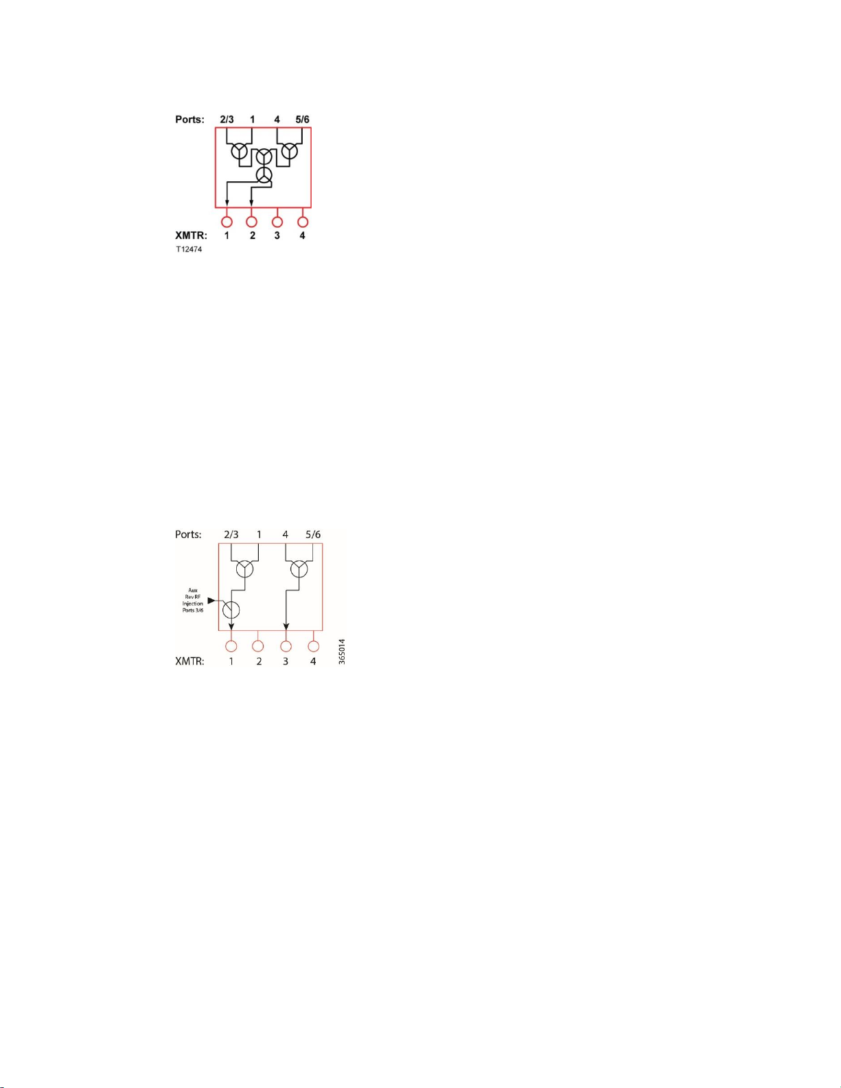
Reverse Configuration Module

4x2 Reverse Configuration Module with Auxiliary Reverse RF Injection Description

The 4x2 Reverse Configuration Module with auxiliary reverse RF injection combines reverse inputs from Ports 1 and 2/3 and routes them to Transmitter 1; it also combines reverse inputs from Ports 4 and 5/6 and routes them to Transmitter 3. An RF signal from an external source can optionally be injected and coupled with reverse RF inputs from Ports 3/6 and routed to Transmitter 1.

Note: This module can only be used with an 8-port optical interface board. (There is no transmitter 3 position with a 6-port optical interface board.)

The following diagram shows how this module functions.

4x2 Redundant Reverse Configuration Module Description

The following diagram shows how this module functions.

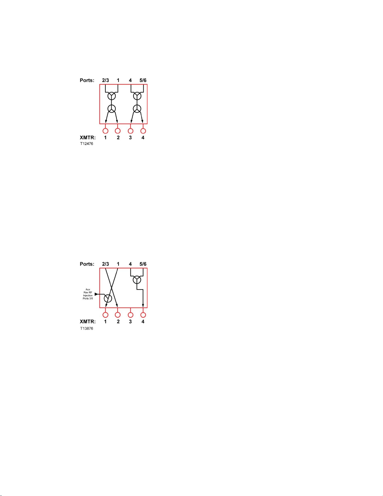
Chapter 2 Theory of Operation

4x3-1, 2, 4 Reverse Configuration Module with Auxiliary Reverse RF Injection Description

The 4x3-1,2,4 Reverse Configuration Module with auxiliary reverse RF injection combines reverse inputs from Ports 4 and 5/6 and routes them to Transmitter 4; it also routes reverse inputs from Port 1 to Transmitter 1 and from Ports 2/3 to Transmitter 2. An RF signal from an external source can optionally be injected at Ports 3/6 and coupled with the reverse RF input from Port 1 and routed to Transmitter 1.

The following diagram shows how this module functions.

4x3-1,3,4 Reverse Configuration Module with Auxiliary Reverse RF Injection Description

The 4x3-1,3,4 Reverse Configuration Module with auxiliary reverse RF injection combines reverse inputs from Ports 1 and 2/3 and routes them to Transmitter 1; it also routes reverse inputs from Port 4 to Transmitter 3 and from Ports 5/6 to Transmitter 4. An RF signal from an external source can optionally be injected at Ports 3/6 and coupled with the reverse RF inputs from Ports 2/3 and 1 and routed to Transmitter 1.

The following diagram shows how this module functions.

Reverse Configuration Module

4x4 Reverse Configuration Module with Auxiliary Reverse RF Injection Description

The 4x4 Reverse Configuration Module with auxiliary reverse RF injection routes reverse inputs from Port 1 to Transmitter 1, from Port 2/3 to Transmitter 2, from Port 4 to Transmitter 3, and from Port 5/6 to Transmitter 4. An RF signal from an external source can optionally be injected and coupled with reverse RF inputs from Ports 3/6 and routed to Transmitter 1.

Note: This module is typically installed when using EDR multiplexing digital reverse modules. Since the digital reverse module occupies the physical space that transmitters 3 and 4 normally occupy in the node base, this reverse configuration module is typically used with a 6-port optical interface board.

The following diagram shows how this module functions.

Chapter 2 Theory of Operation

Optical Interface Board (OIB)

Optical Interface Board Description

The Optical Interface Board (OIB) provides all interconnections between the modules in the housing lid of the 1.2 GHz GS7000 Node. The modules in the housing lid include the optical receiver, optical transmitter, power supply, and status monitoring/local control modules. Each module in the lid plugs directly into the OIB through a connector header or row of sockets. Input attenuator pads are provided on the OIB for each optical receiver in the housing lid. Output attenuator pads are provided on the OIB for each optical transmitter in the housing lid. All RF and power cables running between the housing lid and base also plug into the OIB.

The OIB is field replaceable. All optical modules, power supplies, RF cables, power cables, and OIB mounting screws must be removed in order to remove the OIB from the housing lid.

The upstream status monitoring signal goes through LPF then splits. Splitter output 1 goes through a 17dB coupler into transmitter 1 input. Splitter output 2 goes through a plug-in attenuator pad, a 17dB coupler and into transmitter 2 input.

The purpose of the attenuator (AT9) is to terminate the upstream status monitoring signal going into transmitter 2 when either the node is segmented or EDR transmitter is in use. When the node is configured in either segmented or EDR mode, a 75 dB pad must be placed in the Tx2 SM Term.

This solution resolves the issue of transmitting and receiving duplicate copy of the upstream signal from transponder at the CMTS.

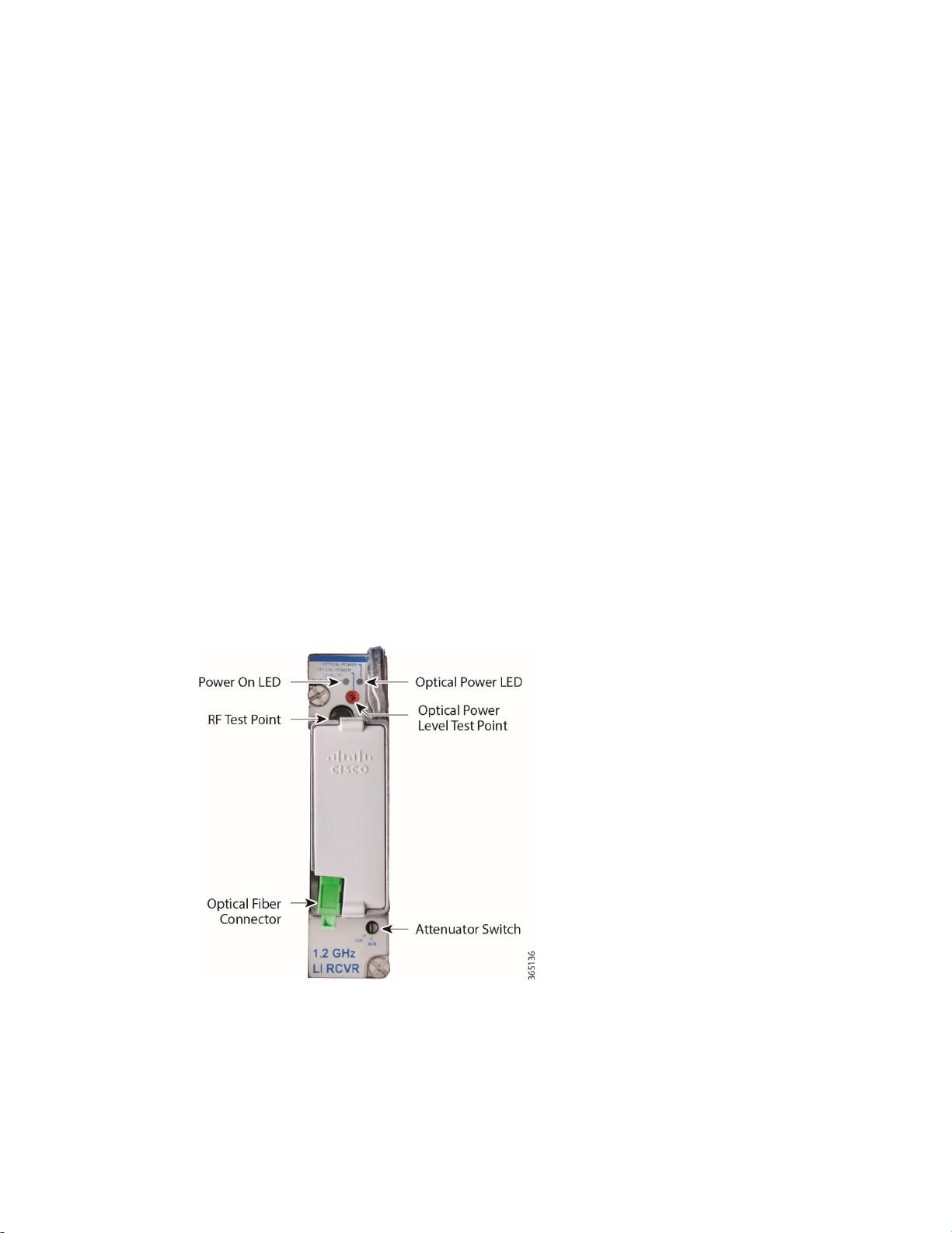
Optical Receiver Module

Optical Receiver Module Description

The optical receiver module takes in optical signals and puts out forward band RF signals. The module cover has a sliding tray incorporated into it allowing the receivers fiber pigtail to be spooled up and contained within the receiver module. This greatly improves fiber management within the node.

The optical receiver modules plug directly into the optical interface board via a connector header and are secured in place with two screws. Input attenuator pads are provided on the optical interface board for each receiver mounted in the housing lid.

All optical receiver test points are provided and are accessible through holes in the module housing. The optical power test points for the optical receiver module has a scaling ratio of 1 V = 1 mW. A -20 dB RF power test point is accessible through the front panel.

The optical receiver module has an optical power LED to indicate the presence of optical power that is either above or below the specified range. ON indicates optical power is within operating limits and OFF indicates that optical power is below the alarm threshold.

The optical power level into the optical receiver module is monitored by the status monitor or local control module. When the node is setup for redundant optical receiver operation, a digital signal is generated by the status monitor or local control module to switch between the primary and redundant optical receiver module in the forward configuration module.

Chapter 2 Theory of Operation

There are two types of the receiver module: Standard Input Optical Receiver and Low Input Optical Receiver.

The optical input range for the low input receiver is 0.1 w to 0.63 w (-10 dBm to -2 dBm). Compared to the standard input optical receiver (the optical input range is -6 dBm to +2 dBm (0.25 w to 1.58 w)), the low input optical receiver can work with lower optical input level, in order to support fiber deep applications.

Optical Receiver Module

The illustration below is Low Input Receiver RF Output Level and Transmitter OMI:

29.0

29.5

30.0

30.5

31.0

31.5

32.0

32.5

33.0

33.5

34.0

34.5

35.0

35.5

36.0

36.5

2.25% 2.50% 2.75% 3.00% 3.25% 3.50% 3.75% 4.00%

Minimum

RF Output

Level

(dBmV)

-6dBm Optical Input Power

Transmitter OMI per Channel

1310nm 1550nm

21.0

21.5

22.0

22.5

23.0

23.5

24.0

24.5

25.0

25.5

26.0

26.5

27.0

27.5

28.0

28.5

2.25% 2.50% 2.75% 3.00% 3.25% 3.50% 3.75% 4.00%

Minimum

RF Output

Level

(dBmV)

-6dBm Optical Input Power

Transmitter OMI per Channel

1310nm 1550nm

Rx Switch in 0 dB Setting:

The illustration below is Low Input Receiver RF Output Level and Transmitter OMI: Rx Switch in -8 dB Setting:

For the detailed information about the low input optical receiver, please refer to the latest GS7000 Data Sheet.

Chapter 2 Theory of Operation

Optical Receiver Module Diagram

The following diagram shows how the optical receiver module functions.

Optical Analog Transmitter Modules

Optical Analog Transmitter Module Descriptions

The optical analog transmitter module takes in reverse band RF signals and puts out optical signals. The 1.2 GHz GS7000 Node is designed to work specifically with the existing mid gain, temperature compensated DFB optical transmitters. Other mid and high gain optical transmitters may be installed in the 1.2 GHz GS7000 Node with varying effects on the overall node specifications. The new module cover fits on all existing optical transmitters. This module cover has a sliding tray incorporated into it allowing the transmitters fiber pigtail to be spooled up and contained within the transmitter module. This greatly improves fiber management within the node.

The optical transmitter modules plug directly into the optical interface board via a connector header and are secured in place with two screws. Output attenuator pads are provided on the optical interface board for each transmitter mounted in the housing lid.

RF test points are accessible through holes in the module housing. The optical power test point for the optical transmitter module has a scaling ratio of 1 V = 1 mW. A -20 dB RF power test point is accessible through the module top cover.

The top cover contains a status monitor LED. Each optical transmitter module laser power indicator turns off when the laser power output falls outside the alarm threshold. It is on (green) when within the alarm threshold.

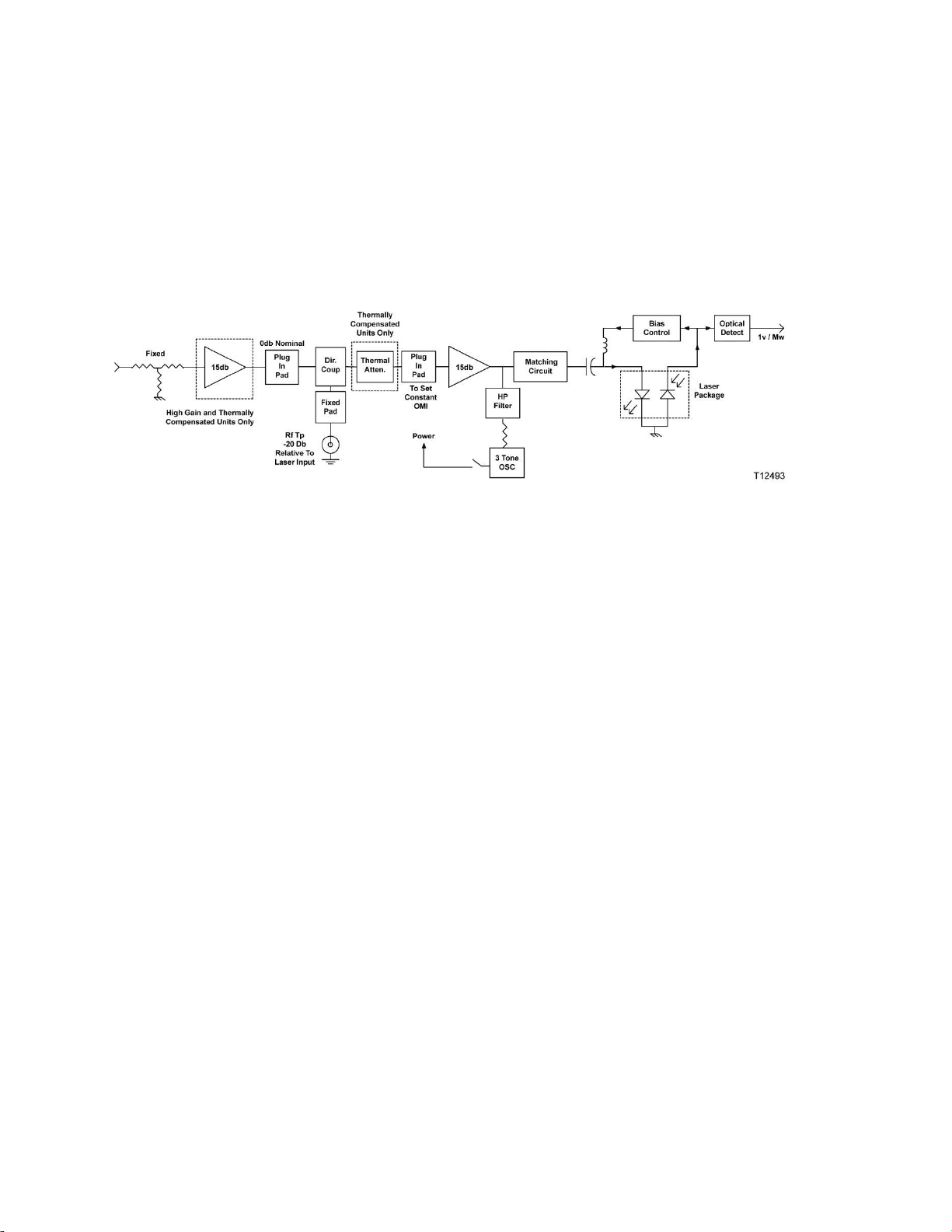
Chapter 2 Theory of Operation

Optical Analog Transmitter Module Diagram

This illustration shows how the optical analog transmitter module functions.

Optical Amplifier (EDFA) Modules

Part Number

Description

GS7K-GFEDFA-17L=

17 dBm gain flattened low gain EDFA

GS7K-GFEDFA-17H=

17 dBm gain flattened high gain EDFA

GS7K-GFEDFA-21L=

21 dBm gain flattened low gain EDFA

Optical Amplifier Module Descriptions

Erbium-doped fiber amplifier modules are available in two categories: broadcast and narrowcast (gain-flattened). Broadcast EDFAs are used for the amplification of broadcast signals which are carried by a single optical channel anywhere between 1530 nm and 1565 nm. (Gain-flattened) EDFAs are used for the amplification of multiple optical channels. For uniformity of performance, EDFAs need to be gain flattened in the designated operating wavelength range between 1536 nm and 1562 nm.

Broadcast EDFAs are available in 17 dBm, 20 dBm, and 22 dBm versions. Narrowcast (gain-flattened) EDFAs are available in 17 dBm, 20 dBm, and 21 dBm versions to fit any architecture for requirements like DWDM narrowcasting.

Both broadcast and (gain-flattened) EDFAs can be operated in constant power and constant gain modes. The default setting for a broadcast EDFA is constant power mode, while the default setting for a (gain-flattened) EDFA is constant gain mode.

The table below lists the part number and description of the new gain-flattened EDFA:

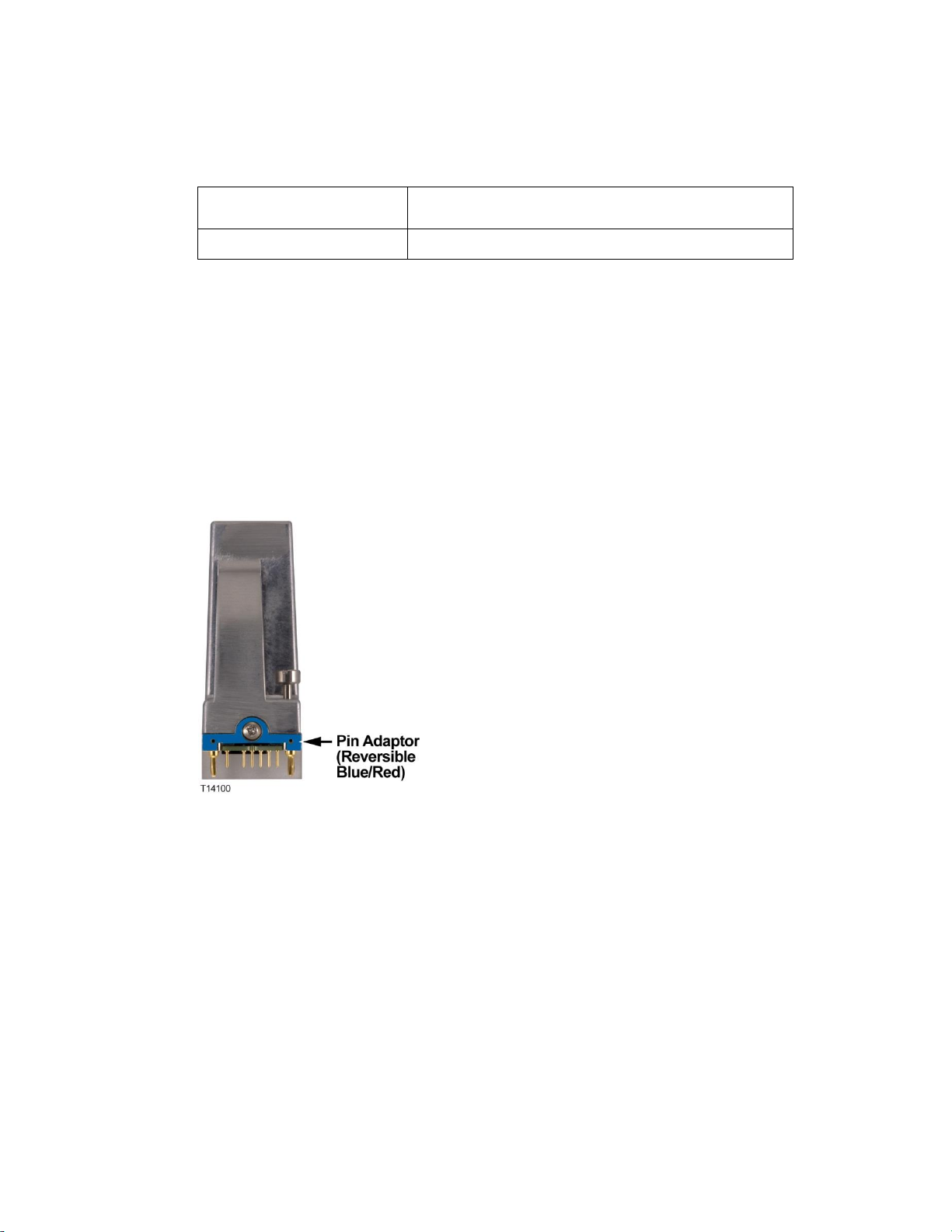
Chapter 2 Theory of Operation

Part Number

Description

GS7K-GFEDFA-21H=

21 dBm gain flattened high gain EDFA

EDFA modules are single-wide, single-output devices. Each module is connected to one input fiber and one output fiber through optical fiber connectors on the side of the module housing. The modules can be mounted in either receiver or transmitter slots on the optical interface board in the node lid using a reversible pin adaptor. The pin adaptor is used to adapt the module to the connector arrangement for a transmitter slot or a receiver slot, which are different. To mount the module in a transmitter slot the red side of the pin adaptor must face out. To mount the module in a receiver slot the blue side of the pin adaptor must face out.

Refer to Optical Amplifier and Optical Switch Module Pin Adaptor (on page 128) for pin adaptor installation instructions.

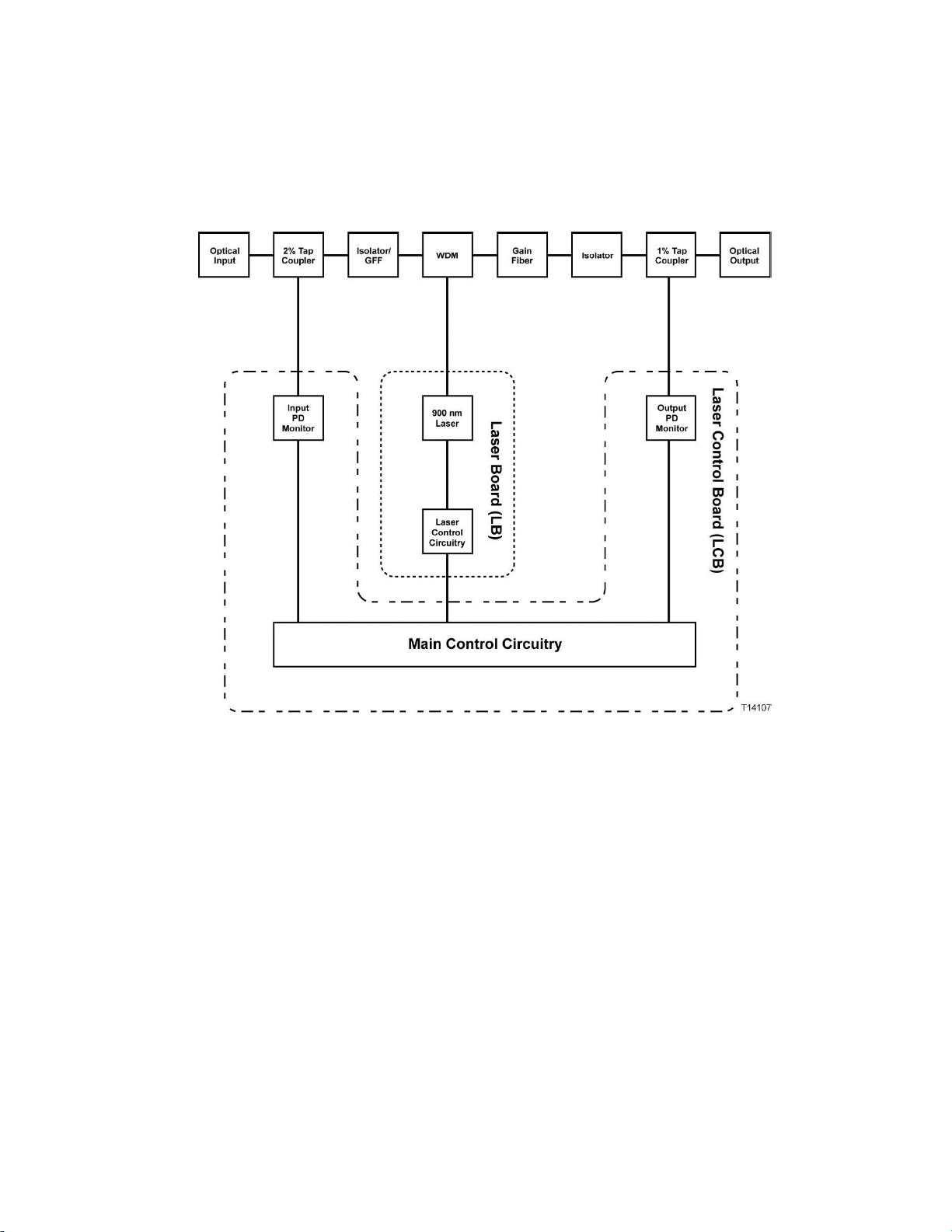
Optical Amplifier (EDFA) Modules

Optical Amplifier Module Diagram

The following block diagram shows how the optical amplifier module functions.

Optical Amplifier Operating Parameters

This section is a reference for the operating parameters of the EDFA. The EDFA is configured through the Status Monitor/Local Control Module in the housing lid. Refer to the GS7000 Hub/Node Status Monitor/Local Control Module Installation and Operation Guide, part number OL-29937, for complete instructions on configuring the EDFA.

Configurable Parameters

The following table defines the configurable parameters for the EDFA.

Chapter 2 Theory of Operation

Param Name

Products

Function

Default Value

Min

Typical

Max

Step

Unit

Mode

All

Sets operating mode of amplifier

[A]

Constant Gain (0) Constant Power (1)

Enable

All

Enables or disables amplifier

Off(0)

Off(0) On(1)

Set Power

BCST 17

Sets optical output level [B]

0.1

dBm

BCST 20

Sets optical output level [B]

0.1

dBm

BCST 22

Sets optical output level [B]

0.1

dBm

GF 17

Sets optical output level [B]

0.1

dBm

GF 21

Sets optical output level [B]

0.1

dBm

Set Gain

BCST 17

Sets gain level in Constant Gain Mode [A][B]

0.1

BCST 20

Sets gain level in Constant Gain Mode [A][B]

0.1

BCST 22

Sets gain level in Constant Gain Mode [A][B]

0.1

GF 17L

[A] 7 5 7 9

0.1

dB GF 17H

[A]

0.1

dB GF 21L

[A]

11 9 11

0.1

dB GF 21H

[A]

0.1

[A] For the Broadcast amplifier, the default is Constant Power. For the (gain-flattened) amplifier, the default is Constant Gain.

[B] In Constant Power mode only.

Optical Amplifier (EDFA) Modules

Operating Status Parameters

Parameter Name

Function

Typical Value

Units

Optical Input Power

Optical input power

5.0

dBm

Output Power

Optical output power

19.5

dBm

Laser Temperature

Laser temperature

25.0

degC

Laser Bias Current Limit

Laser operating current limit

0.825

A Laser Bias Current

Laser operating current

0.625

TEC Current

Thermoelectric cooler current

0.25

Module Temperature

Module temperature

26.5

degC

Laser On Time

Time the laser has been on

1.0

Hrs

Alarm Name

Major High

Minor High

Minor Low

Major Low

Values

Typical Value

Hysteresis

Units

Laser Bias Current

-0.001

-0.010

Alarm

0.625

0.001

Optical Output Level

1.0

0.7

-0.7

-1.0

Alarm

0.1

dBm

Input Power [1]

[5]

Alarm

0.1

dBm

Laser Temperature [1][4]

20.0

15.0

-15.0

-20.0

Alarm

25.0

1.0

degC OIB Voltage

Status [1][2]

Alarm

Internal Power Status [1][3]

Alarm

The following table defines the monitored operating parameters for the EDFA.

Alarm Parameters

The following table defines the alarm parameters for the EDFA.

Chapter 2 Theory of Operation

Alarm Name

Major High

Minor High

Minor Low

Major Low

Values

Typical Value

Hysteresis

Units

Laser Enabled Status [1]

Alarm

[1] This alarm sets the unit to the safe state. In the safe state, the amplifier is turned

Product Type

Major High

Minor High

Minor Low

Major Low

Values

Typical Value

Hysteresis

Units

17.0 / 20.0 /21.0 dBm Low Gain

45.0

25.0

-8.0

-10.0

Alarm

-7.0

0.1

dBm

17.0 / 20.0 /21.0 dBm High Gain

45.0

25.0

-13.0

-15.0

Alarm

-12.0

0.1

dBm

Product Type

Major High

Minor High

Minor Low

Major Low

Values

Typical Value

Hysteresis

Units

17.0 / 20.0 /21.0 dBm

Low/High Gain

45.0

25.0

-10.0

Alarm

5.0

0.1

dBm

Product Type

Major High

Minor High

Minor Low

Major Low

Values

Typical Value

Hysteresis

Units

off causing the optical amplifier output to be disabled.

[2] This alarm tests for presence of +24V, -6V from the OIB.

[3] This alarm indicates the state of the internal voltages (+24V, +5.0V, Vref).

[4] See following for laser nominal set point temperature based on module temperature.

[5] See next table for input power alarm values.

Input Power Alarm Parameters

The following tables define the input power alarm parameters for the EDFA.

(Gain-flattened) EDFA - Constant Gain Mode (Default)

(Gain-flattened) EDFA - Constant Power Mode

Broadcast EDFA - Constant Power Mode (Default)

Optical Amplifier (EDFA) Modules

17.0/20.0/22.0 dBm

45.0

25.0

-10.0

Alarm

5.0

0.1

dBm

Product Type

Major High

Minor High

Minor Low

Major Low

Values

Typical Value

Hysteresis

Units

17.0/20.0/22.0 dBm

45.0

25.0

-13.0

-15.0

Alarm

-12.0

0.1

dBm

Broadcast EDFA - Constant Gain Mode

Laser Temperature Set Point Adjustment

In an effort to reduce EDFA power consumption, laser temperature set point is changed based on EDFA module temperature. Typically, the laser temperature set point is set at 25°C. When module temperature is greater than 60°C and less than 10°C, laser temperature set point is adjusted.

Hot Condition (Module Temperature > 60° C)

For module temperature less than 60.0°C, laser set point temperature is set at 25°C. For every degree of module temperature greater than 60°C, laser set point temperature is also increased by that amount until module temperature reaches 70°C, then laser temperature set point is fixed at 35°C. For example, if module temperature is 64°C, laser set point temperature is 29°C. If module temperature is 85°C, laser set point temperature is 35°C.

Cold Condition (Module Temperature < 10° C)

For module temperature greater than 10°C, laser set point temperature is set at 25°C. For every degree of module temperature less than 10°C, laser set point temperature is also decreased by that amount until the module temperature reaches -5°C, then laser temperature set point is fixed at 10°C. For example, if module temperature is

-4°C, laser set point temperature is 11°C. If module temperature is -25°C, laser set point temperature is 10°C.

Chapter 2 Theory of Operation

Optical Switch Module

Optical Switch Module Description

The optical switch module is used for switching the input of an EDFA module from a primary signal to a backup or secondary signal. The switch operates in the 1550 nm wavelength range since its application is high power/long haul systems that employ EDFAs.

The switch has two operating modes: manual and automatic. In automatic mode, the switch can be triggered by a loss of light. The loss of light activation triggers the switch when the light level drops below the threshold value set by the operator. In manual mode, the switch can be triggered through the Local Control Module (LCM).

The module mounts in receiver or transmitter slots on the optical interface board in the node lid using a reversible pin adaptor. The pin adaptor is used to adapt the module to the connector arrangement for a transmitter slot or a receiver slot, which are different. To mount the module in a transmitter slot the red side of the pin adaptor must face out. To mount the module in a receiver slot the blue side of the pin adaptor must face out.

Refer to Optical Amplifier and Optical Switch Module Pin Adaptor (on page 128) for pin adaptor installation instructions.

Optical Switch Module

Optical Switch Module Diagram

The following block diagram shows how the optical switch module functions.

Optical Switch Operating Parameters

This section is a reference for the operating parameters of the optical switch. The optical switch is configured through the Status Monitor/Local Control Module in the node. Refer to the GS7000 Hub/Node Status Monitor/Local Control Module Installation and Operation Guide, part number OL-29937, for complete instructions on configuring the optical switch.

Chapter 2 Theory of Operation

Switch Operation

Primary Input

Secondary Input

Alarms

Optical Switch

Path A Optical Power > ThresholdA (default)

Path B Optical Power > Threshold B [1]

None

Switch to Path A

Path A Optical Power < ThresholdA (default)

Path B Optical Power > Threshold B [1]

Loss of Input Light at Path A

Switch to Path B Optical Power

Path B Optical Power > Threshold B [1]

Path B Optical Power < Threshold B [1]

Loss of Input Light at Path B

Switch to Path A

Path A Optical Power < ThresholdA (default)

Path B Optical Power < Threshold B [1]

Both Dark

Switch to Path A Optical Power

Path B Optical Power > ThresholdB (User Setting)

Path A Optical Power > ThresholdA [1]

None

Switch to Path B

Path B Optical Power < ThresholdB (User Setting)

Path A Optical Power > ThresholdA [1]

Loss of Input Light at Path B

Switch to Path A Optical Power

Path B Optical Power > ThresholdB (User Setting)

Path A Optical Power < ThresholdA [1]

Loss of Input Light at Path A

Switch to Path B

Path B Optical Power < ThresholdB (User Setting)

Path A Optical Power < ThresholdA [1]

Both Dark

Switch to Path B Optical Power

Parameter

Function

Default Value

Values

Min

Max

Step

Unit

Mode

Automatic or manual mode

Auto(0)

Manual(1)

Threshold B

Switching threshold, input optical power at input B

5.0 -10.0

14.0

0.1

dBm

The following table describes the optical switch function.

[1] Hysteresis Amplitude (default 1.0 dB) is the value above which the input optical power must rise for the switch to begin sequence to return to the primary switch position. Hysteresis Amplitude is a user configurable parameter.

Configurable Parameters

The following table defines the configurable parameters for the optical switch.

Optical Switch Module

Parameter

Function

Default Value

Values

Min

Max

Step

Unit

Threshold A

Switching threshold, input optical power at input A

5.0 -10.0

14.0

0.1

dBm

Hysteresis Amplitude

Hysteresis Amplitude: The value (in dB relative to the switching threshold) above which the input optical power must raise for the switch to begin the hysteresis timer before restoring primary switch position. Only applies if Revert is On.

1.0 0.5

9.5

0.1

Hysteresis Time

Hysteresis Time: The length of time, in seconds, that primary optical power must remain above the restore threshold before switch is allowed to revert to primary position. Only applies if Revert is On.

60 0

600 1 sec

Revert

On (1) allows switch to revert to primary position after optical power restored. In Off (0), switch will remain in backup (non-primary) position.

On(1)

Off(0)

On(1)

Primary Optical Input

Selects the primary optical input

PathA(0)

PathB(1)

na Switch

Position

Selects the Normal switch position

PathA(0)

PathB(1)

Chapter 2 Theory of Operation

Operating Status Parameters

Parameter Name

Function

Typical Operating Range

Units

Switch Position

Read optical switch position

(Calibrated at 1550 nm only)

PathA/PathB

state

Path A Optical Power

Input optical power on Path A

(Calibrated at 1550 nm only)

-10 to 14

dBm

Path B Optical Power

Input optical power on Path B

-10 to 14

dBm

Module Temp

Module temperature

Ambient temp + 7

degC

Switch Temp

Switch temperature

Ambient temp + 7

degC

Alarm Name

Error Condition

Values

Hysteresis

Loss of Input Light at Path A

Optical input at path A is less than the switching threshold at path A

Minor Alarm(0)

Ok(1)

[1]

Loss of Input Light at Path B

Optical input at path B is less than the switching threshold at path B

Minor Alarm(0)

Ok(1)

[1]

Both Dark

Loss of light at both inputs

(Loss of Input Light at Path A and Loss of Input Light at Path B)

Major Alarm(0) [2]

Ok(1)

No Switch

Optical switch failed to change states when commanded

Major Alarm(0) [2]

Ok(1)

Power Supply OK

Failure of external power supply rails

Major Alarm(0) [2]

Ok(1)

Excessive Input Optical Power

Optical input at Path A or optical input at Path B is greater than or equal to 24 dBm

Major Alarm(0) [2]

Ok(1)

The following table defines the monitored operating parameters for the optical switch.

Alarm Parameters

The following table defines the alarm parameters for the optical switch.

Optical Switch Module

[2] In some cases this may display as Fault (0).

Chapter 2 Theory of Operation

Local Control Module

Overview

A local control module and a status monitor are available for the 1.2 GHz GS7000 Node and Hub Node. A status monitor consists of a local control module with a transponder core module installed in the housing. The same housing is used for both units. The units perform the following function:

 Local Control Module - controls redundancy and forward segmentation, and

configures the modules

 Status Monitor - adds status monitoring capability to the local control module  DOCSIS capability

Status Monitor Description

The status monitor is HMS compliant and provides node monitoring and control capability at the cable plant's headend. The following node voltages and signals are monitored and their status reported to the headend by the status monitor.

 Receiver optical input level (all receivers)  Transmitter optical output level (all transmitters)  AC power presence and peak voltage (for split AC powering cases, AC

power from both sides of node housing is monitored)

 DC voltages from both primary and redundant power supplies  Optical amplifier operating parameters  Optical switch operating parameters

Commands are sent from the headend to the status monitor. The status monitor communicates serially with the RF amplifier module to control the optional forward band redundancy switches on the forward configuration module, the reverse band 6 dB (wink) attenuators on the reverse amplifier PWB, and the reverse band on/off switches on the reverse amplifier PWB.

Note: Configuration parameters for the transponder core module, such as IP address, can be changed using the PC-based GS7000 ViewPort software.

Local Control Module

Note: The transponder core module can be seen through the Heart Beat/Receive/Error indicator cutout in the cover.

Local Control Module Description

The local control module locally monitors the following node voltages and signals:

 Receiver optical input level (all receivers)  Transmitter optical output level (all transmitters)  AC power presence and peak voltage (for split AC powering cases, AC

power from both sides of node housing is monitored)

 DC voltages from both primary and redundant power supplies  Optical amplifier operating parameters  Optical switch operating parameters

The local control module communicates serially with the RF amplifier module to control the optional forward band redundancy switches on the forward

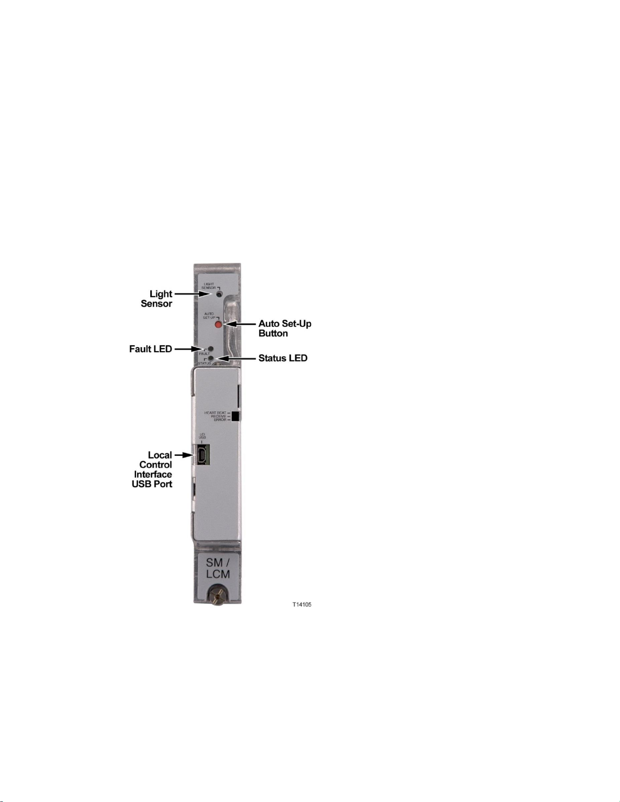
Chapter 2 Theory of Operation

configuration module. It is a low-cost module that plugs into the status monitor connectors on the optical interface board.

The local control module is equipped with a USB port to allow local control of the optional forward band redundancy switches, the reverse band 6 dB (wink) attenuators, the reverse band on/off switches, the optical switch, and optical amplifiers through the PC-based GS7000 ViewPort software. All parameters monitored by the local control module can be displayed and reviewed using ViewPort.

Note: The local control module can be upgraded to a status monitor through the addition of a transponder core module. The transponder core module plugs directly

onto the local control module’s PWB. The mechanical housing for the status monitor

and the local control module are the same. The Heart Beat, Receive, and Error indicator LEDs are only present if the transponder module is installed.

Power Supply Module

Power Supply Module Description

The power supply module converts a quasi-square wave, 50 – 60 Hz AC input voltage into four well-regulated DC output voltages. The supply is an off-line, switched-mode power supply with a large operative input range. This reduces service outages by converting long duration AC surges into load power. The power supply is a constant power device, meaning that it automatically adjusts its internal operating parameters for the most efficient use of the different levels of input voltage and current it will receive within the cable plant.

The DC output voltages generated by the power supply, at given load currents, are shown below:

+24.5 VDC @ 6.2 Amps +8.5 VDC @ 1.0 Amps +5.5 VDC @ 1.3 Amps

-6.0 VDC @ 0.8 Amps

Test points are provided on top of the power supply module for AC input and all output DC voltage rails.

Chapter 2 Theory of Operation

The power supply module plugs directly into the optical interface board, no external cables are required.

A 1.2 GHz GS7000 Node can be configured with one or two power supplies. AC input voltage can be routed to both power supplies commonly from any node output port. In addition, AC input voltages can be routed in a split fashion to the two power supplies. AC input voltages from the left half of the node (output ports 1 – 3) can be routed to power supply 1 independent of AC input voltages from the right half of the node (output ports 4 – 6) being routed to power supply 2. Each of the power supplies output voltage rails is diode OR'd within the supply. This creates common DC powering circuits when multiple supplies are present in the node.

Power Supply Module

CAUTION:

The life of the equipment may be reduced if configured to draw more than the recommended level of power from the power supplies.

Equipment

Type

Maximum Power Draw (Watts)

Typical Power Draw (Watts)

Transmitter

1310 nm dfb, analog CWDM

4.1

3.4 Transmitter

analog DWDM

5.4

4.8

Standard Input Receiver

operating

4.1

3.9

Standard Input Receiver

standby

0.5

0.4 Low Input Receiver

operating

4.1

3.85

Low Input Receiver

standby

0.5

0.4

EDFA

17 dBm

4.5 4 EDFA

20 dBm

7 5 EDFA

22 dBm

9 7 Optical Switch

2 1.5

Status Monitor/ Local Control Module

2.6

0.9 RF Amplifier

4-way forward segmentable

72.8

72.9

Node Power Limitations

Nodes and hub nodes must be configured in a manner that prevents potential thermal overloads. Heat generated by the node can reduce the life of the equipment.

Two power supplies can provide a maximum power level of 100 watts to the node or hub node. The RF amplifier uses the majority of the available power. Maintain the total power consumption of all modules in the housing within these guidelines to minimize the heat generated. Find the optimal configuration by summing the power consumption of the RF amplifier plus the other individual modules in the housing using the following table.

Important: Do not populate the housing with any combination of modules that would draw more than the available power of 100 watts.

The following table lists the modules and their respective power consumption.

Chapter 2 Theory of Operation

1:1 EDR Transmitter

< 3 2:1 EDR Transmitter

< 7

Introduction

This chapter describes the installation of the 1.2GHz GS7000 Node.

3 Chapter 3

Installation

In This Chapter

 Tools and Test Equipment ................................................................... 66

 Node Housing Ports ............................................................................. 68

 Strand Mounting the Node ................................................................. 69

 Pedestal or Wall Mounting the Node ................................................ 72

 Fiber Optic Cable Installation ............................................................. 74

 RF Cable Installation ............................................................................ 82

 Applying Power to the Node .............................................................. 85

Chapter 3 Installation

Tools and Test Equipment

Fastener

Torque Specification

Illustration

Housing closure bolts

5 to 12 ft-lbs (6.8 to 16.3 Nm)

Test point port plugs

Housing plugs

5 to 8 ft-lbs (6.8 to 10.8 Nm)

Strand clamp mounting bracket bolts

5 to 8 ft-lbs (6.8 to 10.8 Nm)

Pedestal mounting bolts

8 to 10 ft-lbs (10.8 to 13.6 Nm)

Module securing screws

(Tx, Rx, PS, and SM/LCM modules)

25 to 30 in-lbs (2.8 to 3.4 Nm)

Required Tools and Test Equipment

The following tools and equipment are required for installation.

 Torque wrench capable of 5 to 12 ft-lbs (6.8 to 16.3 Nm)  4-inch to 6-inch extension for torque wrench  1/2-inch socket for strand clamp bolts and cover bolts  1/4-inch flat-blade screwdriver  #2 Phillips-head screwdriver  Long-nose pliers  1/2-inch deep-well socket for seizure connector  True-rms digital voltmeter (DVM)  EXFO FOT 22AX optical power meter with adapters  Optical connector cleaning supplies  Optical connector microscope with appropriate adapters for your optical

connectors

Node Fastener Torque Specifications

Be sure to follow these torque specifications when assembling/mounting the node.

Tools and Test Equipment

Fastener

Torque Specification

Illustration

RF Amplifier assembly shoulder screws (cross head screw)

18 to 20 in-lbs (2.0 to 2.3 Nm)

Seizure nut

2 to 5 ft-lbs (2.7 to 6.8 Nm)

RF cable connector

Per manufacturer instructions

Fiber optic cable connector

20 to 25 ft-lbs (27.1 to 33.9 Nm)

Chapter 3 Installation

Node Housing Ports

The following illustration shows the location of available RF ports, fiber ports, and test points on the 1.2 GHz GS7000 Node housing.

Notes:

 External test points are only active on models with the "Amplifier Type 3 -

External Test Points Activated" option.

 When replacing test point port plugs, torque from 5 to 8 ft-lbs (6.8 to 10.8 Nm).

Strand Mounting the Node

WARNING:

Be aware of the size and weight of the node while strand mounting. Ensure that the strand can safely support the node’s maximum weight. A fully loaded 1.2 GHz GS7000 Node weighs over 50 lbs (22.7 kg).

Ensure the ground area below the installation site is clear of personnel before hoisting the node. If possible, block off walkway below the hoisting area to prevent pedestrian traffic during hoisting.

Failure to observe these admonishments can result in serious injury or death.

Description

The following procedure explains how to install the 1.2 GHz GS7000 Node on a strand (aerial installation). Strand mounting allows street-side access to the housing.

Procedure

Follow this procedure to mount the housing to a strand. The housing does not need to be opened for strand installation.

1 Check the strand size. The minimum strand diameter should be 5/16 inch. 2 Attach the strand clamp brackets to the housing in the position shown in the

following illustration. Use a torque wrench tightens the strand clamp bracket bolts from 5 ft-lb to 8 ft-lbs (6.8 to 10.8 Nm).

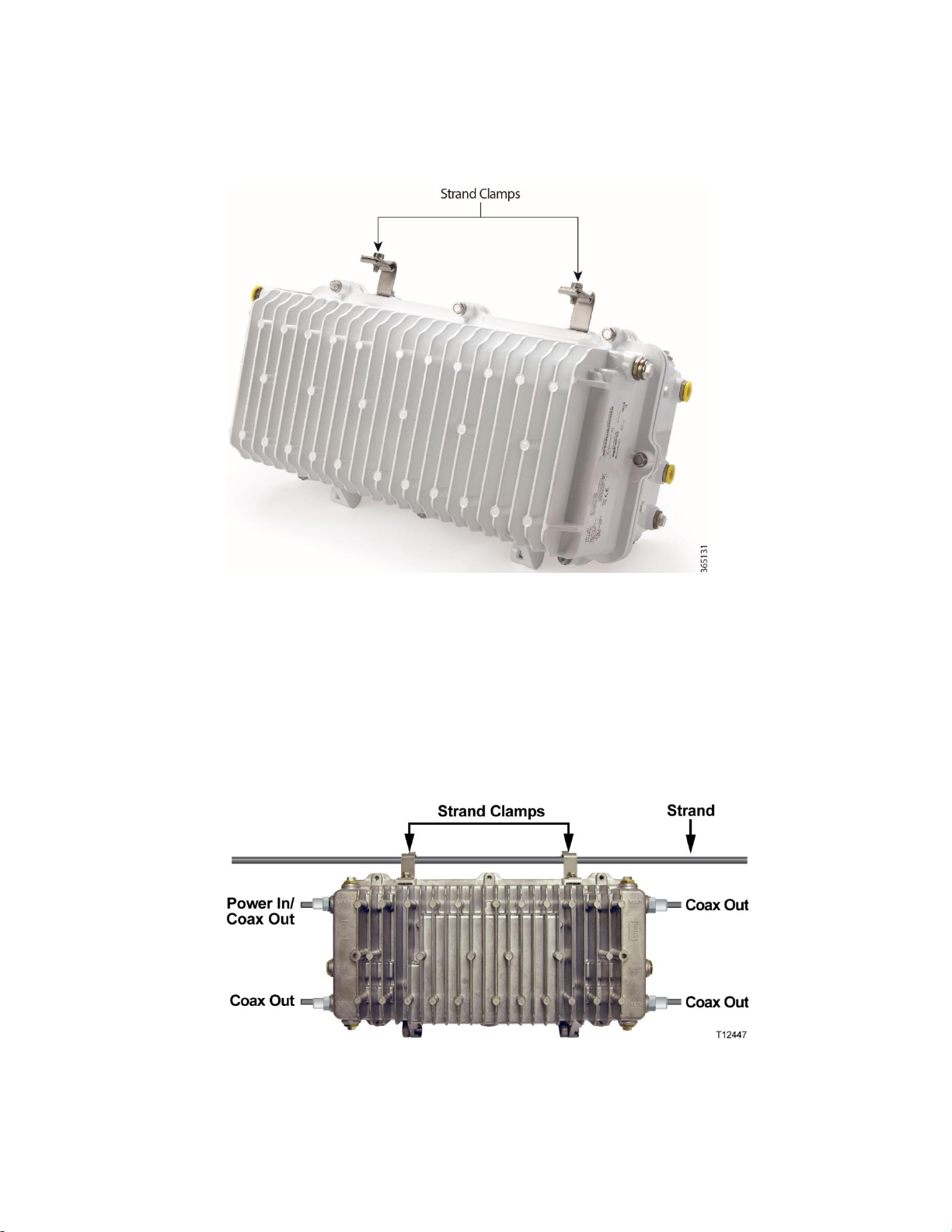
Chapter 3 Installation

3 Loosen the strand clamp bolts to separate the clamps enough to insert the strand,

but do not remove them. Then lift the housing into proper position on the strand.

4 Slip the clamps over the strand and finger-tighten the clamp bolts. This allows

additional side-to-side movement of the housing as needed.

5 Move the housing as needed to install the coaxial cable and connectors. See the

illustrations below for an example

Powered from Left

Powered from Right

Strand Mounting the Node

Note: If supplying power to the node through a main output port, a power inserter must be installed to inject the AC voltage onto the RF signal.

6 Use a torque wrench and a 1/2-inch socket to tighten the strand clamp bolts

from 5 ft-lb to 8 ft-lbs (6.8 to 10.8 Nm).

Note: A slight tilt of the face of the housing is normal. Cable tension will cause the housing to hang more closely to vertical.

7 Connect the coaxial cable to the pin connector according to the pin connector

manufacturer’s specifications.

8 Continue to Fiber Optic Cable Installation (on page 74) and RF Cable

Installation (on page 82).

Chapter 3 Installation

Pedestal or Wall Mounting the Node

WARNING:

Be aware of the size and weight of the node while mounting. A fully loaded 1.2 GHz GS7000 Node weighs over 50 lbs (22.7 kg).

Ensure that proper handling/lifting techniques are employed when working in confined spaces with heavy equipment.

Failure to observe these admonishments can result in serious injury or death.

Description

Two mounting holes on the housing allow pedestal or wall mounting.

Procedure

Follow this procedure for pedestal or wall mounting.

1 Remove the cover of the pedestal. 2 Remove the self-tapping bolts from the strand clamps, if previously installed,

Pedestal or Wall Mounting the Node

and set the bolts and strand clamps aside.

3 Position the 1.2 GHz GS7000 Node horizontally in the enclosure and allow for

free flow of air around it. Inadequate airflow could cause the node to exceed thermal parameters. Line up the bolt holes on the bottom of the housing with the mounting holes on the pedestal bracket provided by the pedestal manufacturer.

Important: The node housing must be mounted horizontally, as shown, to ensure proper airflow over the housing cooling fins. Do NOT mount the node housing vertically.

4 Secure the node housing to the pedestal bracket using the strand clamp bracket

bolts you removed in step 2. Insert the bolts into the mounting holes. Use the strand clamps as spacers if necessary. Torque the bolts from 8 ft-lb to 10 ft-lb (10.8 Nm to 13.6 Nm).

5 Connect the coaxial cable to the pin connector according to connector

manufacturer’s specifications.

6 Ground the equipment in accordance with local codes and regulations. 7 Continue to Fiber Optic Cable Installation (on page 74) and RF Cable

Installation (on page 82).

Chapter 3 Installation

Fiber Optic Cable Installation

Connector/Adapter Number

Fiber Color Code

Connects to

Blue

forward receiver 1

Orange

forward receiver 2

Green

reverse transmitter 1

Brown

reverse transmitter 2

Slate

spare

White

spare

Red

spare

Black

spare

Overview

The 1.2 GHz GS7000 Node can accept a fiber optic cable connector from either the right or left side of the housing, or both. The fiber optic cable(s) carries forward and reverse optical signals.

This procedure assumes a specific type of connector as an example. Your connector may be different from the one shown in these illustrations. Be sure to install the connector according to the connector manufacturer’s instructions.

Important: Fiber optic cable installation is a critical procedure. Incorrect installation can result in severely degraded 1.2 GHz GS7000 Node performance. Be sure to

carefully follow fiber connector manufacturer’s instructions. See Care and Cleaning of Optical Connectors (on page 134).

Color Code

Fiber connectors and adapters are labeled with the following color code.

Note: This is only a suggested setup. Your fiber assignment may be different. Refer to your network diagrams to verify your color code.

Fiber Optic Cable Installation

Fiber Management System

The fiber management system is made up of a fiber tray and a fiber routing track. The fiber tray provides a convenient location to store excess fiber and up to two WDM modules in the node. The tray is hinged to allow it to move out of the way during the insertion of the fibers and for installation or replacement of the node power supplies. The fiber routing track provides a channel for routing fiber pigtails to their appropriate optical modules as well as a location to snap in unused fiber connectors for storage.

The following illustration shows the design of the fiber tray.

Note: Fibers are spooled in a counterclockwise direction in the tray.

The following illustrations show the location and layout of the fiber tray and track in the housing lid.

Chapter 3 Installation

Fiber Optic Cable Installation

Note: Power supplies are removed in the previous illustration for clarity.

WARNING:

Laser light hazard. The laser light source on this product emits invisible laser radiation. Avoid direct exposure. Never look into the end of an optical fiber or connector. Failure to observe this warning can result in eye damage or blindness.

IF...

THEN...

fiber optic cable is factory installed

splice fiber pigtail of optical fiber input cable to your splice enclosure and continue to RF Cable Installation.

fiber optic cable is not installed

go to step 2.

Procedure

Install fiber optic cable as described below.

 Do not apply power to this product if the fiber is unmated or unterminated.  Do not stare into an unmated fiber or at any mirror-like surface that could reflect

light that is emitted from an unterminated fiber.

 Do not view an activated fiber with optical instruments.

1 The first step depends on whether the fiber optic cable is factory installed or not.

2 Select the right or left fiber connection port for use and remove its sealing plug.

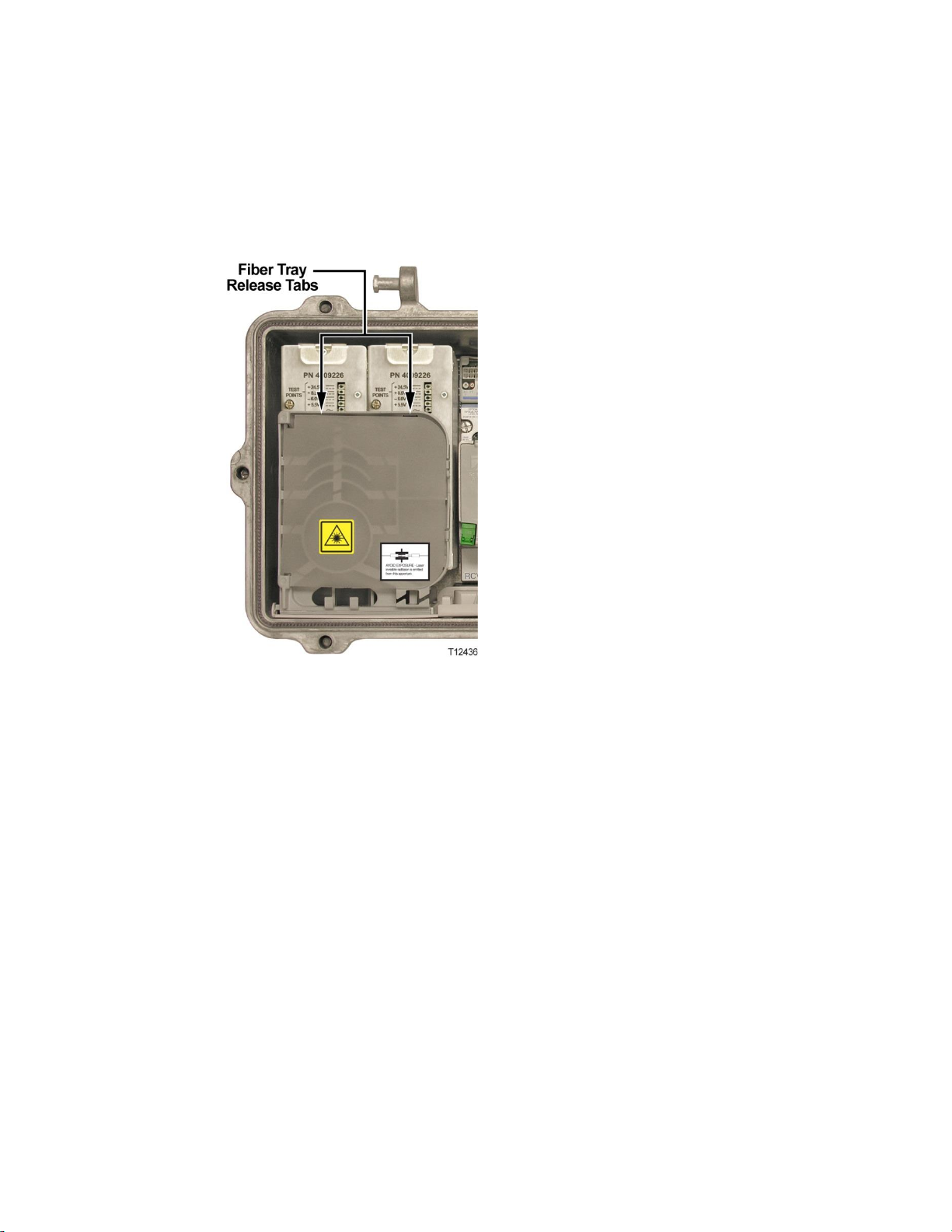
Chapter 3 Installation

3 Push in the two release tabs at the top of the fiber tray and swivel the top of the

fiber tray up and back to allow a clear view of the fiber routing channel below.

4 One at a time, carefully insert fibers with attached connectors through the fiber

connection port, the fiber channel, and then up and through the fiber entry point in the bottom of the fiber tray. Do not bend or kink fibers. Though not necessary, you can also remove the power supplies and open the fiber routing channel cover for additional access.

Fiber Optic Cable Installation

Note: If using the alternate (right-side) fiber connection port, you have to route the fibers through the fiber channel in the fiber track located underneath the

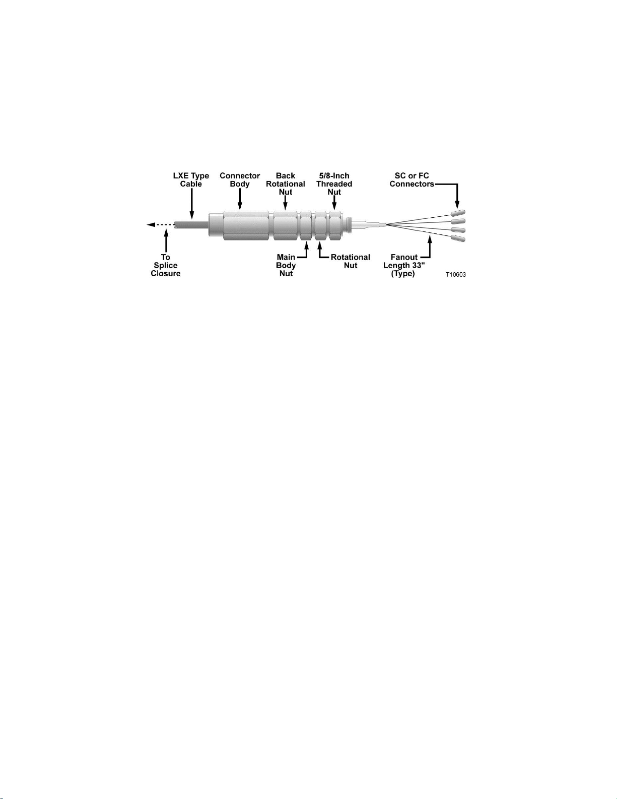
Chapter 3 Installation

unused fiber holders.

5 Hold the connector body to prevent rotation of the connector or fibers.

6 Carefully thread the 5/8-inch threaded nut into the threaded hole of the fiber

port. Tighten to 20 to 25 ft-lbs (27.1 to 33.9 Nm).

7 Firmly tighten the rotational nut against the 5/8-inch threaded nut. 8 Push heat shrink tubing over the connector and fiber port and shrink in place. 9 Identify individual fibers according to their color code and determine to which

receiver or transmitter module each fiber will connect.

10 Pivot the fiber tray back down and snap it into place on top of the power supply

with its locking tabs.

11 Open the fiber tray cover and carefully wind the fibers around the spool in a

counterclockwise direction. Be sure to leave enough fiber so that each connector can reach its intended module. Note that different diameter spool paths are provided to properly adjust the fiber length.

Cisco GS7000 User Manual

Specifications and Main Features

Frequently Asked Questions

User Manual