


Vibration equipment division
www.cemb.com
CEMB S.p.A.
Via Risorgimento, 9
23826 MANDELLO del LARIO (Lc) Italy
*Translation of the original instructions
N600
Dual chaNNel spectrum aNalyzer
aND BalaNciNg
u
se aND maiNteNaNce iNstructioN maNual


Vibration equipment division
N600 - Ver.2.2 09/2015
General Index
1. General descrIptIon 5
1.1 Standard acceSSorieS 5
1.2 optional acceSSorieS 5
1.3 connectionS 6
1.4 Battery 7
1.5 General advice 7
2. General layout 8
2.1 KeyS/ButtonS on the control panel 8
2.2 General purpoSe functionS 10
2.2.1 Functions associated with the measuring phase 10
2.2.2 Function “other Functions...” 10
2.2.3 Functions operating on the graphs 11
2.2.4 T
o save measurements 13
2.2.5 T
o capture and save displayed images 14
3. Home screen (menu) 15
4. setup mode 16
4.1 SenSor Setup 16
4.1.1 type oF sensor 16
4.1.2 sensitivity oF the sensor 17
4.1.3 photocell 17
4.2 MeaSureMent Setup 18
4.2.1 unit oF measure 18
4.2.2 measurement type 18
4.2.3 unit oF Frequency 19
4.2.4 max Frequency 19
4.2.5 no. oF lines 19
4.2.6 no. oF means 19
4.3 General Setup 20
4.3.1 date 20
4.3.2 time 20
4.3.3 language 20
4.3.4 measurement system 20
4.3.5 time zone 20
4.3.6 updating oF Firmware 20
5. VIbrometer mode 22
5.1 viBroMeter - MeaSureMent Screen 22
5.1.1 direct printing oF the vibration value (optional) 22
5.2 MonitorinG in tiMe 23
5.3 MonitorinG in Speed 23
6. FFt (Fast FourIer transForm) analyzer mode 25
6.1 SpectruM analySiS (fft) 25
6.2 harMonic curSor 25
6.3 WaveforM function 26
6.4 triGGer Setup 26

N600 - Ver.2.2 09/2015
6.4.1 modes 27
6.4.2 channel 27
6.4.3 threshold 28
7. balancer mode 29
7.1 Selection of the BalancinG proGraM 30
7.1.1 new program - balancing setup 30
7.1.1.1 number oF planes 30
7.1.1.2 Filter accuracy 30
7.1.2 load program From archive 31
7.1.3 use current program 31
7.1.4 copy archive to usb key 31
7.2 caliBration Sequence 32
7.3 execution of MeaSureMent 33
7.3.1 test weight 33
7.4 unBalance MeaSureMent and calculation of the correction 34
7.5 SplittinG of correction WeiGht 36
7.6 SavinG of a BalancinG proGraM 37
8. data manaGer mode 38
8.1 open exiStinG project 38
8.2 chanGe Selected pointS 39
8.3 neW project 40
8.4 iMport projectS froM
USB
Key 40
8.5 export projectS to uSB Key 40
8.6 delete projectS 41
9. arcHIVe FunctIon 42
9.1 load ScreenShot 42
9.2 delete ScreenShotS 43
10. cemb n-pro proGram (optIonal) 44
10.1 SySteM requireMentS 44
10.2 inStallation of the SoftWare 44
10.3 inStallation of driverS for uSB coMMunication With the n100, n300 inStruMentS
(for verSion 1.3.4 or earlier) 45
10.4 inStallation of driverS for uSB coMMunication With the n100 and n300 inStruMentS
(for 46
verSion 1.3.5 and later only) 46
10.5 activatinG the SoftWare 47
10.6 uSe of the SoftWare 48
10.6.1 Function bar 48
10.7 General SettinGS 49
10.8 readinG data froM the n100 or n300 inStruMent 50
10.9 data recordS iMported froM the n100 or n300 inStruMent 51
10.10 R
eadinG data froM the n600 inStruMent 51
10.11 diSplayinG data preSent in the recordS 52
10.12 Specific functionS for the SpectruM GraphS 52
10.13 SynchronouS viBration value MeaSureMent (only for n100 and n300 inStruMentS) 53
10.14 BalancinG data (only for n300 and n600 inStruMentS) 54
10.15 Generation and printinG of certificateS (reportS) 54
10.16 GeneratinG and printinG Multiple MeaSureMent certificateS (Multi-report) 55

Vibration equipment division
N600 - Ver.2.2 09/2015
Appendix A
specIFIcatIons 5
6
Appendix B
eValuatIon crIterIa 5
8
Appendix C
a rapId GuIde to InterpretInG a spectrum 6
2
Appendix D
laser sensor For cemb n Instruments 6
8
Appendix E
InFormatIon related to tHe creatIon oF customIsed templates (models) For certIFIcates Generated by
cemb n-pro soFtware 69
Attachment: Balancing accuracy for rigid rotors

N600 - Ver.2.2 09/2015

Vibration equipment division
5
N600 - Ver. 2.2 09/2015
1. General descrIptIon
The N600 instrument is supplied, together with its accessories, in a special case. It is advisable, each time the instrument is
used, to place back it in its case in order to avoid risk of damage during transit.
1.1 standard accessorIes
• No. 2 velocity transducers 100mV/g
• No. 2 transducer connection cables L 2.5 m
• No. 1 heavy duty spiral cable L 2 m
• No. 2 magnetic bases Ø 25 mm
• No. 2 probes
• No. 1 250.000 Cpm Hi-speed, laser photocell complete with upright and magnetic base
• No. 1 roll of reecting paper
• No. 1 USB stick for data transfer
• Angle rule
• Battery charger
• Universal plug
• Case complete with carry strap
• User manual
1.2 optIonal accessorIes
• Bluetooth thermal printer for direct printing of certicates on normal or adhesive thermal paper
• Protective cover
• Acceleration transducer type DM-40 complete with connection cable and magnetic base
• Proximity sensor type ARA-18 complete with stand, cable and magnetic base
• Connection cable for transducers L 5 m
• Extension cable, length 10 metres, for transducers
• Extension cable, length 10 metres, for photocell
• CEMB ADS software for data storage and management
aFter connecting the printer via bluetooth, wait For about 5 seconds to allow completion oF the automatic re-
cognition and initialization procedure. only at this point will it be possible to make a print-out by pressing relative
key F
3 .
6
N600 - Ver. 2.2 09/2015
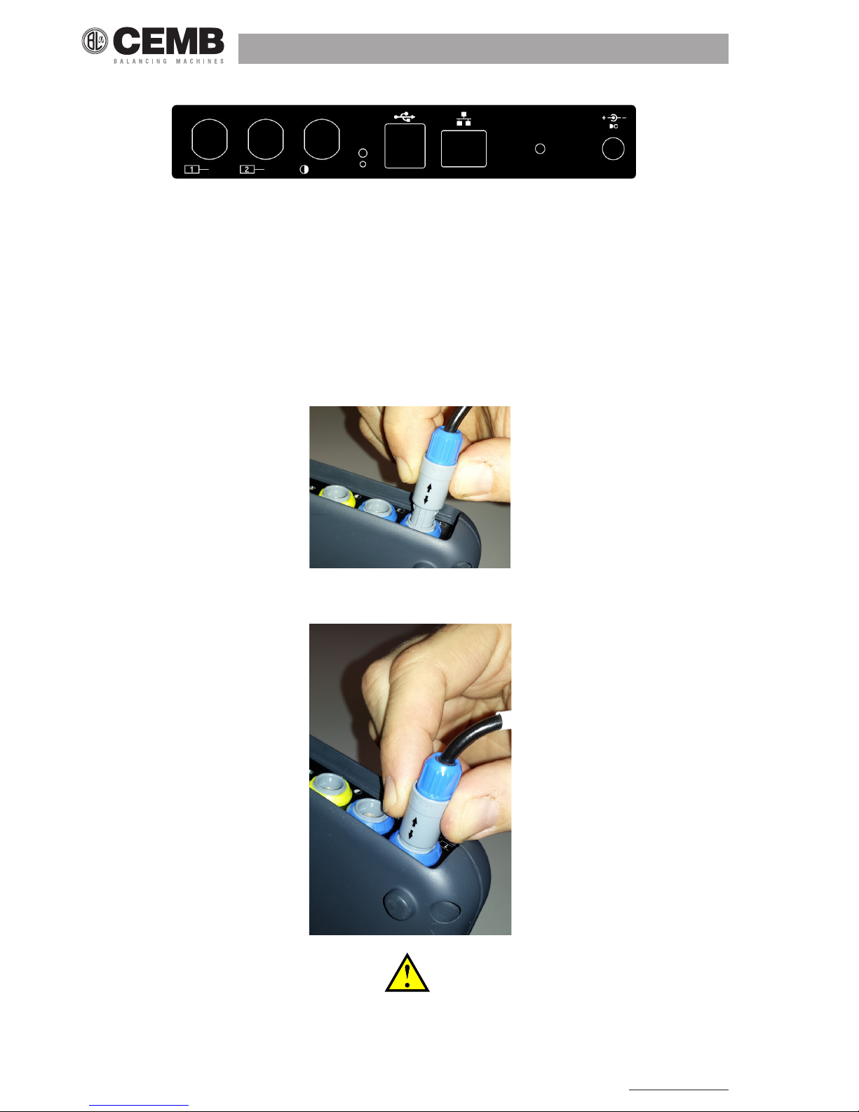
1
23
4
5
6
7
1.3 connectIons
1 Battery charger
2 Internal heat dissipation area (electronics)
3 Network port (useful to connect the instrument to a PC and share a folder for data exchange between the two)
4 2 USB ports type A (master)
5 Instrument reset button
6 Battery charge indication led
7 Photocell input
8 2 inputs, measuring channels
To connect the sensors and photocell, merely plug the connector in the corresponding socket, pushing it until it clicks into
place; make sure that the safety connection is correctly aligned as shown in the gure.
Instead, to extract the connector, press its end part (blue or yellow) and at the same time pull the main body (grey), in order
to release it.
————————————————————————————————————————————————————
warnInG!
aVoId pullInG tHe connector wItH Force beFore releasInG It as descrIbed aboVe,
otHerwIse tHere would be rIsk oF damaGInG It.
————————————————————————————————————————————————————

Vibration equipment division
7
N600 - Ver. 2.2 09/2015
1.4 battery
The N600 instrument is provided with a built-in rechargeable lithium battery, which allows autonomy of more than eight hours
under normal operating conditions of the instrument.
The battery status is indicated by an icon in the upper right hand corner of the screen.
battery fully charged
battery partly charged
battery almost at (battery life remaining when this appears is approx. one hour)
battery at: recharge within 5 minutes
In these conditions, any still active measurements are interrupted and therefore not yet saved.
————————————————————————————————————————————————————
warnInG!
It Is stronGly recommended to recHarGe tHe battery wItH tHe Instrument swItcHed oFF: as recHarGInG Is completed wItHIn
less tHan FIVe Hours sucH precautIon preVents tHe battery cHarGer From beInG connected For an excessIVely lonG perIod
oF tIme (max. 12 Hours).
————————————————————————————————————————————————————
————————————————————————————————————————————————————
warnInG!
tHe lItHIum battery Is able to wItHstand tHe recHarGInG-dIscHarGInG cycles, eVen on a daIly basIs, wItHout problems but It
could become damaGed IF allowed to be Fully dIscHarGed. For tHIs reason It Is adVIsable to recHarGe tHe battery at least
once eVery tHree montHs, eVen In tHe case oF extended Idle perIod
————————————————————————————————————————————————————
as the greater consumption is due to the back lighting oF the lcd display, the latter is switched oFF automatically
aFter two minutes iF no button is pressed. the pressing oF any button (except For and those oF the alphanu meric keypad) is suFFicient to switch the back lighting on again.
1.5 General adVIce
Keep and use the instrument far from sources of heat and strong electromagnetic elds (inverters and high-power electric
motors). Measurement accuracy could be impaired by the connection cable between the transducer and instrument, there-
fore it is recommended to:
• not allow such cable to have sections in common with power cables;
• prefer a perpendicular arrangement when overlapping power cables;
• always use the shortest possible length of cable; in fact oating lines would act as active or passive antennae.
8
N600 - Ver. 2.2 09/2015
2. General layout
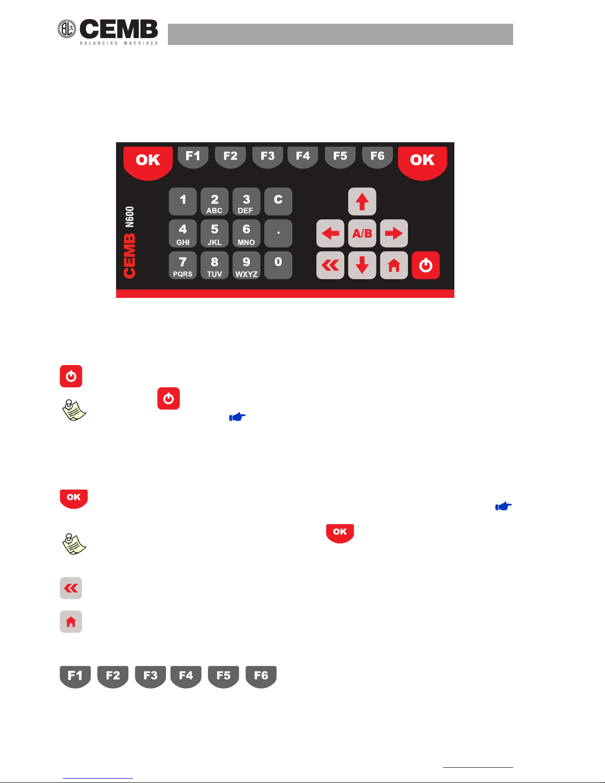
2.1 keys/buttons on tHe control panel
The control panel of the CEMB N600 instrument incorporates a keypad where the various keys or buttons can be subdivided
by function:
► ON / OFF button
Press this button to switch the instrument on; hold it down for at least 3 seconds to switch it off , then release the
button.
aFter pressing , the instrument is ready For use only at the end oF the switching on procedure, signalled by
the appearance oF the home screen (
home screen - menu
).
aFter the insrument has been switched oFF, about 30 seconds must pass beFore it can be switched back on again.
► Buttons for navigating between the pages
When this button is pressed in the setup screen, it conrms the settings selected and allows going onto the next
screen. Instead, in the Measurement screen, it has the function of starting/stopping the actual measurement (
START / STOP THE ACQUISITION).
to Facilitate use oF the instrument also with the leFt hand, the button is located on both sides oF the
display.
When this button is pressed, it causes quitting of the current screen with return to the previous one, without taking
into account any changes (or saves) in the settings
Used for returning to the Main page, from any other page.
► Function keys
Each function key is linked to different functions in the various screens. Such functions are indicated in each individual case
by the buttons shown at the bottom of the display: each function is activated by pressing the function key under it.

Vibration equipment division
9
N600 - Ver. 2.2 09/2015
T
T U
P
Q R
-
0
1
In the setup screens they are used for setting the various parameters, each one being indicated by a number corresponding
to that of the function key to be pressed to modify it.
► Tab key
This key can only be used when two graphs are plotted on the same page; when pressed, it changes the active
graph to which the selected functions will be applied. The active graph can be identied by the symbol loca ted on the right side.
► Arrow keys
When a graph is displayed, these keys increase or decrease respectively the minimum or max. value of the x axis ( ,
) or the y axis ( , ). Instead, when inputting a value for a parameter, they either shift the cursor to the
left or right ( , ) and increase or decrease the value in question ( , ).
► Alphanumeric keypad
This keypad serves for entering alphanumeric characters in the elds which do not allow just default selections. Where it is
possible to enter just numbers, it acts like a normal numeric keypad.
To enter a character, press a key repeatedly to scroll the characters assigned to it (e.g. M N O 6) until the required one is
displayed. The cursor passes on automatically to the next position after a pause of one second, or else after pressing another key.
With it is possible to delete the character to the left of the cursor.
For example, suppose we wish to enter the word “TUR-1” press:
10
N600 - Ver. 2.2 09/2015
an icon indicates whether the upper case style (selectable with ) or lower case (selectable
with
).
► Image capture key
Pressing of this key has the function of capturing the image present on the display and opening a screen which
allows it to be saved ( CAPTURE AND SAVING OF DISPLAYED IMAGES).
2.2 General purpose FunctIons
In addition to many functions, specic for each different purpose and described in relative sections, there are certain general
purpose functions which are described below.
2.2.1 Functions associated with the measuring phase
► Start / Stop acquisition
In all the Measurement screens, acquisition is started by pressing and is subsequently stopped by again pressing
. The active acquisition status is easily to recognize (except in the balancing function) by the presence of a bar indi-
cating level of the input signal to each of the activated channels.
Instead, in the Balancing functions, this status is signalled by an indication of the quality of the measurement in progress
( EXECUTION OF MEASUREMENT).
2.2.2 Function “other Functions...”
When there are more than six functions accessible from a certain screen, there are not enough function keys to correspond
to them; in such cases the key is associatedwith .
Pressing of this key causes substitution of the functions corresponding to with another ve. The original
correspondence can be reset by again pressing .
Vibration equipment division
11
N600 - Ver. 2.2 09/2015
2.2.3 Functions operating on the graphs
► Scale setting
allows selecting the function for modication of the minimum and maximum values of the axes in a
graph; in this way it is possible to display just the zone of greater interest. When activated, the following
sub-functions are made available:
quit the Scale Setting function
preset minimum value of the x axis
preset maximum value of the x axis
preset minimum value of the y axis
preset maximum value of the y axis
sets the axis limits to be coherent with the graph data
The value of the limit selected (x
min
, x
max
, Y
min
or else Y
max
, displayed by white wording on black background), can be increased
or decreased by pressing
, for X axis and , for Y axis.
measurement can be started with also while set scale is activated but it would automatically cause exit
From this Function.
when two graphs are shown both at the same time on the same screen, the scale Functions operate on the active graph
(identiFied by symbol ). to change the active graph, proceed to press the key
.
► Use of the cursor
For easier reading and interpretation of the displayed data, it is possible to introduce a cursor in any graph, provided the
visible region is not blank: this can be done with F2
. A window at the top right corner of the graph contains the
co-ordinates of the point where the cursor lies.
The cursor can be shifted by one step to the right or to the left by using thefollowing keyse F1
or F3
respectively.
For quick reaching of points from the current position, hold down F1 or F3 . With F2 the
cursor is removed.

12
N600 - Ver. 2.2 09/2015
measurement can started with also while the cursor is visible; at the end oF the measurement, the cursor
remains visible.
when two graphs are represented on the same screen simultaneously, it is possible to display the cursor on both
in order to have easier comparisons and assessments. however, pressing oF the Function keys will only have eFFect
on that oF the currently activated graph (identiFied by the symbol ). to change the activated graph, proceed to
press the key.
► Change of display channel
If both measuring channels are enabled, various types of display are possible, namely:
• just graph of channel Ch1
• just graph of channel Ch2
• graphs of channels Ch1 and Ch2 simultaneously
The passing in sequence between the various possibilities is obtained by repeatedly pressing This corresponds in
each case to these options or
► List of peaks
When this function is selected, a table appears with the 10 peaks of highest value present in the zone of the spectrum displayed, and associated with the corresponding frequencies. Their value is calculated by applying an interpolation algorithm to
the FFT graph; this also allows identifying peaks not situated in correspondence to one of the lines of the spectrum.
When F5 is pressed, the system quits this function and again displays the graph (or graphs).
the 10 highest peaks are determined in relation to the highest value present in the spectrum; hence in certain cases
the list could contain less than 10 peaks..

Vibration equipment division
13
N600 - Ver. 2.2 09/2015
iF graphs oF both channels are displayed, the list oF peaks should be calculated For the active one (identiFiable by
the symbol
).
2.2.4 T
o save measurements
The N600 instrument, structured according to a route logic, allows easily saving acquired data; to this end, two different route
types are available ( DATA MANAGER MODE):
• Soft route
• Strict route
If using Soft Route, pressing allows viewing the PROJECT STRUCTURE screen relating to the tree corresponding to the currently active route. All the individual measurement points marked by the symbol
, allow saving the data
several times.
Select the measurement point in which to save the measurement made using the arrows
and , and then press
to save the measurement in the selected point.
If you have done a two-channel acquisition, both channels are automatically saved in the same le.
If using Strict Route, pressing F5
a pop-up will inform you that the measurement has successfully been saved.
the , button, accessible by pressing , allows reloading the measurements previously
processed.
U
sing the arrows and , select the measurement you want to reload (indicated by the date [mm/dd/yyyy]
and time [hh:mm:ss] oF acquisition) and conFirm by pressing the button
.

14
N600 - Ver. 2.2 09/2015
2.2.5 T
o capture and save displayed images
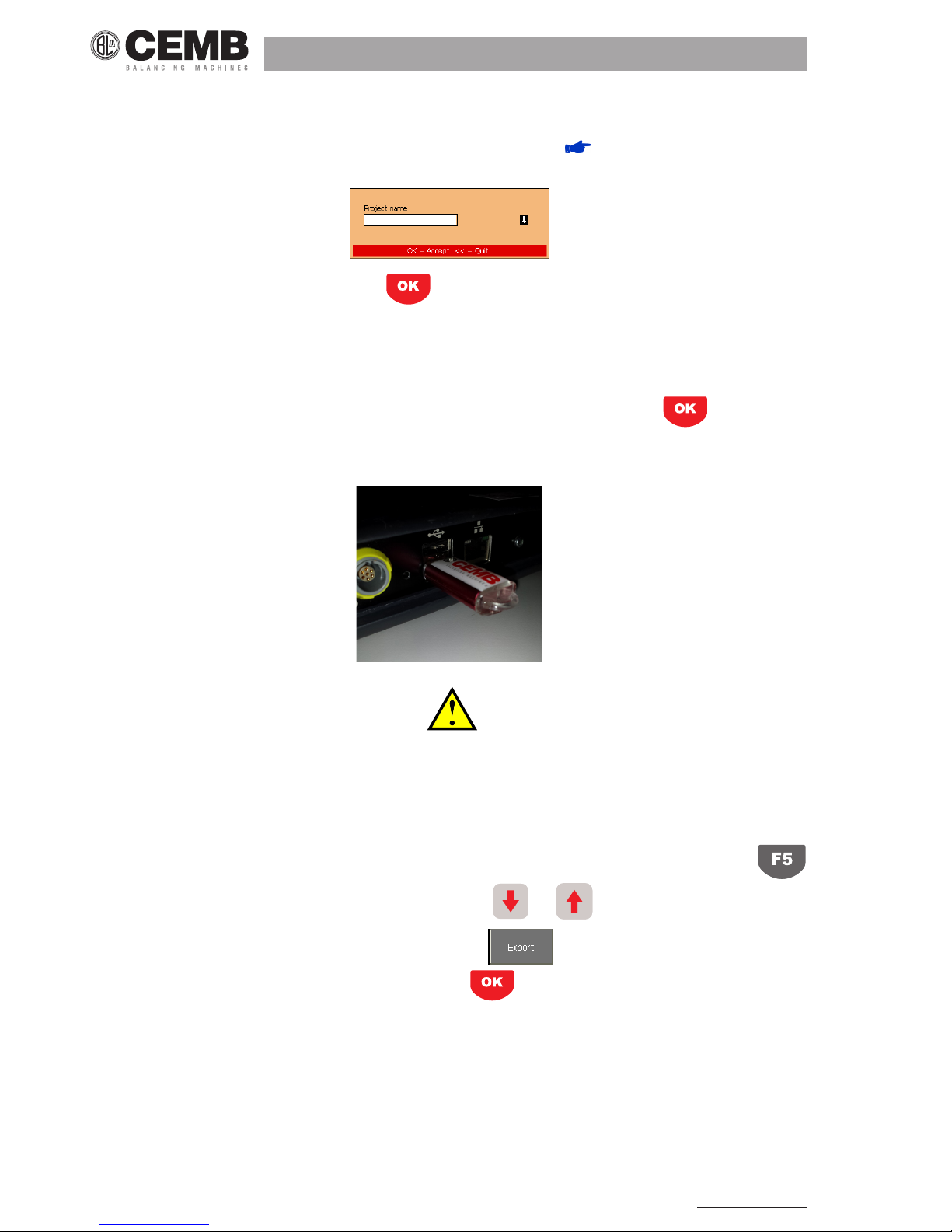
In all screens of the N600 instrument, the image visible on the display can be captured with then saved in png format
in an appropriate archive. This image can be used subsequently if required to accompany documentation produced by the
operator.
Selection of the position where to save can be done with the arrow keys and , then merely press F2
to display a pop-up where to enter the required name, as explained in ALPHANUMERIC KEYPAD.
To delete an image, and clear the corresponding position in the archive, merely press the button F3 .Instead with
F4 it is possible to fully clear the image le.
When pressing the above mentioned buttons, the popup shown below asks you to conrm the operation with the button
or quit with the button .
Finally, pressing F6 , all the image les on the instrument will be copied to a folder called Screenshots, which will
automatically be created on the USB key inserted in the instrument.
E
ach time you want to save new images on the same usb key, ’other subFolders named with the date and time will be
created in the screenshots Folder.
keys
and
, which either increase or decrease by 10 respectively the position selected, can be used
For quick scrolling oF the archive.

Vibration equipment division
15
N600 - Ver. 2.2 09/2015
3. Home screen (menu)
After fully switching on the N600 instrument, it shows its Home screen:
which, besides showing a set of information:
• manufacturer logo and name of the instrument
• serial number (S/N) of the instrument
• current program version
• battery state:
> fully charged
> partly charged
> almost at
> at
> instrument being charged (connection to socket via the battery charger supplied)
as a normal menu, it also proposes and allows selection of the available modes, namely:
► Vibrometer mode
• measurement of the total value and synchronous measurement of vibration
• measurement and memorization of the trend in vibration against variation in time or rotor speed
► FFT (Fast Fourier Transform)
• splitting of the vibration into its component frequencies
• display of waveform of the vibration
► Balancer mode
• balancing of rotors
► Setup mode
• setting of the characteristics of sensors connected to the instrument
• setting of the general operating parameters of the instrument
► Project management
• open an existing project
• modify the measurement points selectable in a project during a eld measurement campaign
• create a new project (Soft Route only)
• import new projects (Soft Route and Strict Route) from USB key
• export projects from the instrument to USB key
• delete existing projects
► Archive
• load a previously stored screenshot

16
N600 - Ver. 2.2 09/2015
• delete one or all the previously stored screenshots
it is possible to return to this screen From any other by pressing
.
4. setup mode
This function allows making all the possible conguration settings on the N600 instrument. More specically, these settings
are:
• Sensor setup: conguration of the sensors that interface with the instrument
• Measurement setup: conguration of the measurement settings
• General setup: conguration of the general operating parameters of the instrument.
4.1 sensor setup
The N600 instrument can be used with different types and models of sensors. Therefore in order to ensure correct measurement, it is necessary to preset exactly the type of sensitivity of the sensors actually connected.
although the instrument can operate correctly with any combination oF sensors, it is advisable to connect sensors
oF the same type and model to the two channels.
4.1.1 type oF sensor
Any one of the following possibilities can be selected:
• OFF : sensor not present (or else channel to be kept switched off)
• ACCEL : accelerometer
• VELOC : velocity sensor
• DISPLC : proximity sensor (non-contact)
it is not possible to set both channels to oFF; at least one oF the two channels should be activated
Vibration equipment division
17
N600 - Ver. 2.2 09/2015
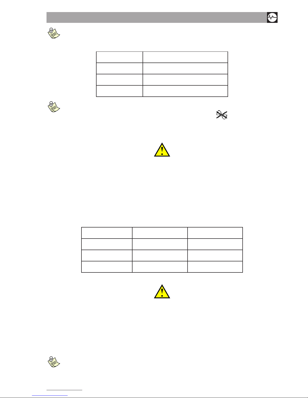
although the required unit oF measurement can diFFer From the natural one oF the sensor, these are the only
combinations are possible.
TYPE OF SENSOR REQUIRED MEASUREMENT
ACCEL acceleration, speed, displacement
VELOC speed, displacement
DISPLC displacement
the n600 instrument is able to determine automatically whether there is no sensor connected to an enabled chan-
nel (i.e. not set to oFF sensors setup) and it signals this by showing the symbol in the vicinity oF the signal
bar oF the corresponding channel (only during measurement). to avoid displaying this symbol, it is advisable to disa-
ble the channel when not used, by setting to oFF.
————————————————————————————————————————————————————
warnInG!
tHe appearance oF tHIs symbol For a cHannel wHere a sensor Is really connected,
could IndIcate a possIble malFunctIon oF tHe sensor or else a problem In connectIon
(e.G. tHe cable could HaVe been sHeared).
In sucH case It Is adVIsable to carry out a Few tests by connectInG a sensor (wHIcH Is known to be operatInG properly) to
tHe cHannel In questIon; IF tHe IndIcatIon persIsts, contact cemb tecHnIcal serVIce.
————————————————————————————————————————————————————
4.1.2 sensitivity oF the sensor
This is the number of volts per unit produced by the sensor: it is expressed for the various types in:
TYPE OF SENSOR SENSITIVITY TYPICAL VALUE
ACCEL mV/g 100
VELOC mV/(mm/s) 21,2
DISPLC mV/µm 4
————————————————————————————————————————————————————
warnInG!
dIFFerent models can HaVe sensItIVIty dIFFerInG From tHe typIcal Values; pay attentIon
wHen takInG tHe correct Value From tHe sensor documentatIon and preset It .
————————————————————————————————————————————————————
4.1.3 photocell
You can set activation of the photocell or its power circuit. Setting the parameter to ON, the photocell will continuously be
powered as soon as it is connected to the instrument.
iF the photocell is not enabled, when you select a program that requires’its use, a pop-up will ask you to activate it.

18
N600 - Ver. 2.2 09/2015
4.2 measurement setup
In the case of analysis using a Soft Route, this function allows making the necessary settings to obtain a correct overall value
measurement via the Vibrometer function as well as highlighting signicant data in the spectrum, separating them from the
ineliminable background noise relating to the FFT function.
I
n the case oF analysis using a strict route, this Function allows checking but not modiFying the parameters set.
the symbol allows identiFying a setup relating to a strict route.
4.2.1 unit oF measure
Select the unit of measure in which you want the vibration measurement to be provided; the options are:
• Acceleration (g) - strengthens the higher frequencies and weakens the lower frequencies
• Speed (mm/s or inch/s)
• Displacement (µm or mils) - strengthens the lower frequencies and weakens the higher frequencies
4.2.2 measurement type
This is the mode in which each component (line) of the spectrum is provided and may be:
• RMS (Root Mean Square):
This is the mean vibration value squared beforehand.
This value is typically used in the European standards, in particular for acceleration or speed measurements.
It is a direct index of the “energy” content of the vibration. In practice, it represents the power the vibration carries with it,
which is discharged onto the supports of the vibrating structure.
• PK (Peak):
This is the maximum value the vibration has reached in a certain time interval.
For purely sinosoidal signals, it is simply equal to the RMS value multiplied by 1.41.
• PP (Peak-to-Peak):
This is the difference between the maximum and minimum values the vibration has reached in a certain time interval; for
purely sinosoidal signals, it is simply equal to the RMS value multiplied by 2.82.
It is normally used for displacement measurements.

Vibration equipment division
19
N600 - Ver. 2.2 09/2015
linee
max
N
f
4.2.3 unit oF Frequency
There are two options:
• Hz - cycles (revolutions) per second
• RPM - revolutions per minute
evidently, there is a relation between the two units: 1 hz = 60 rpm.
4.2.4 max Frequency
This is the maximum frequency involved in the phenomenon under examination; in practice, it is the maximum frequency
viewable in the spectrum. You can choose from the default values 100, 500, 1000, 2500, 5000, 10000 Hz, based on which
the N600 instrument selects the appropriate frequency for data acquisition.
T
he typical choice appropriate For most situations is 1000 hz (60.000 rpm) consistent with what is indicated in iso
10816-1.
normal practice is to check that the maximum Frequency set is at least 20-30 times that oF rotation oF the shaFt
under test. this allows including in the spectrum also the high Frequency zone where bearing-related problems
normally occur.
at parity oF other conditions, choosing a low maximum Frequency (below 1000 hz) results in considerably longer
acquisition and measurement times.
4.2.5 no. oF lines
This parameter denes the number of lines used in the FFT algorithm, in practice related to the resolution in frequency in the
spectrum. This determines how close the frequency of two peaks may be for them to still be distinguished in the FFT graph.
This resolution is equal to:
therefore, in order to keep them constant, if the maximum frequency is increased, also the number of lines must be increased.
It should be pointed out that the time necessary to acquire the correct number of samples is exactly equal to the inverse
of the resolution to which the time necessary to process the data needs to be added. An example of the relation between
resolution and acquisition time is shown in the table below:
Resolution [Hz]
t
Acquisition [
sec
]
5 0,2
2,5 0,4
1,25 0,8
0,625 1,6
0,3125 3,2
it is inadvisable to use a too large number oF lines unless you have a situation where an extreme resolution is es-
sential.
T
his would in Fact translate into an increase in calculation time and the space required For data saving,
oFten without adding particular inFormation. a reasonable choice would be to use 200, 400 or 800 lines at most,
making sure that you set a maximum Frequency consistent with the situation under examination.
4.2.6 no. oF means
This is the number of spectrums/data that needs to be calculated and averaged in order to enhance measurement stability.
Four means are more than sufcient for normal vibration measurements on rotating machines.
Pressing
the settings are conrmed.
20
N600 - Ver. 2.2 09/2015
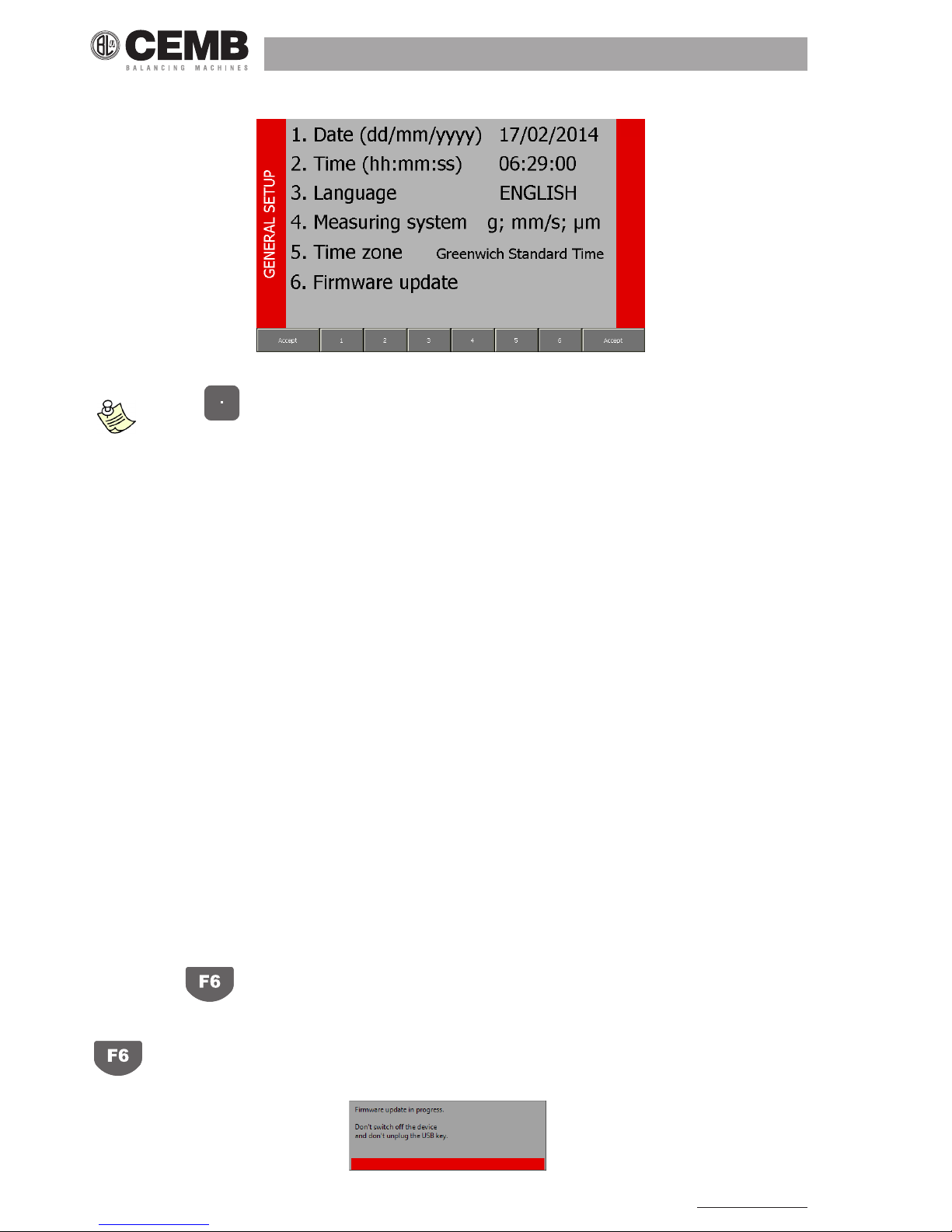
4.3 General setup
The parameters for general use of the instrument should be preset in this page.
when the key is pressed, the system inFo pop-up appears, containing Full inFormation concerning the
system. strike any key to close this window.
4.3.1 date
Use the alphanumeric keypad to enter the date in the format DD/MM/YYYY.
4.3.2 time
Use the alphanumeric keypad to enter the date in the format HH:MM:SS.
4.3.3 language
Select one of the possible languages:
• ITALIANO
• ENGLISH
• DEUTSCH
• FRANÇAIS
• ESPAÑOL
4.3.4 measurement system
The units of measure for the acceleration, speed and displacement values can be the following respectively:
• g; mm/s; μm : metric units
• g; inc/s; mils : imperial units
4.3.5 time zone
Allows setting the time zone. This setting is important if the instrument is associated with the CEMB Advanced Diagnostic
Software for data processing.
4.3.6 updating oF Firmware
Pressing of key does not set any parameter, but it does allow updating the program (rmware) inside the instrument,
if this proves necessary. Each new rmware version consists of a le with the extension fmw, which should be copied in the
main directory on the USB key supplied. Merely insert the pendrive in one of the USB ports of the instrument, then press
to start the automatic updating procedure, at the end of which the pop-up:

Vibration equipment division
21
N600 - Ver. 2.2 09/2015
signals successful transfer of the le and requests switching the instrument off, then on again to complete the operation.
————————————————————————————————————————————————————
cautIon!
updatInG oF tHe FIrmware Is a delIcate operatIon, wHIcH could last a Few mInutes. It sHould be carrIed out by payInG careFul
attentIon to tHe InstructIons supplIed In order not to cause malFunctIons or data loss; For tHIs reason, a conFIrmatIon Is
requested beFore actIVatInG tHIs procedure.
————————————————————————————————————————————————————
Only the rmware obtained directly from CEMB Technical Service should be used. It is advisable to remove the USB key
before rebooting the instrument.
If using invalid rmware, the following pop-up will appear:
————————————————————————————————————————————————————
warnInG!
IF tHe automatIc updatInG operatIon Is not perFormed successFully, contact cemb
tecHnIcal serVIce, cItInG tHe type oF error sIGnalled.
————————————————————————————————————————————————————

22
N600 - Ver. 2.2 09/2015
1
3
8
4
5
2
6
7
9
5. VIbrometer mode
One of the simplest, but at the same time most signicant information in vibration analysis, is the overall value of the actual
vibration. In fact, this is very often the rst parameter to be considered when evaluating the operating conditions of a motor,
fan, pump, machine tool.
Appropriate tables allow discrimination between an optimum state and a good state, or from an allowable, tolerable, nonpermissible or even a dangerous one. ( APPENDIX B - EVALUATION CRITERIA).
In certain situations instead, it could be interesting to know the values of modulus and phase of the synchronous vibration
(1xRPM), i.e. corresponding to the speed of rotation of the rotor.
The vibrometer mode is designed to make this type of measure and also makes available two monitoring functions, for
observing the trend of vibration plotted against time or against variation in rotor speed.
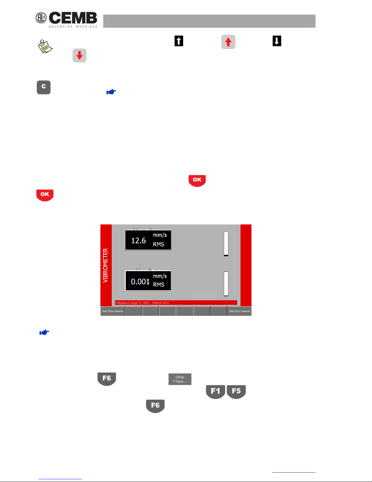
5.1 VIbrometer - measurement screen
The Measurement page supplies a series of information, organized as shown in the gure:
1. measurement information: indicates unit of the sensor (A, V or D) and any conversion made to supply the overall value
(e.g. A→V means that the measurement is made with an accelerometer, but the vibration is supplied in speed)
2. channel measured
3. overall value of the vibration
4. unit of measurement
5. type of measurement
6. value of the synchronous vibration
7. phase of the synchronous vibration
8. speed rotation of rotor
9. signal level bar
the values obtained in this mode can be reused to evaluate the operating status oF the instrument by using, For
example, the tables and graphs given in appendix B oF this manual.
The default measurement is that of the total vibration value, but by pressing F4 it is possible to switch to measu-
rement of the synchronous value: in this mode, information appears concerning the modulus, phase and speed of rotation.
Pressing of F4 allows return to measurement of the overall. value.
to perForm a synchronous measurement, it is necessary to connect the photocell and make sure that it is positio-
ned correctly (
SPEED MONITORING).
5.1.1 direct printing oF the viBration value (optional)
By connecting the portable printer supplied (optional) then pressing F3 it is possible to print directly in eld the
vibration values displayed in the VIBROMETER PAGE.
Vibration equipment division
23
N600 - Ver. 2.2 09/2015
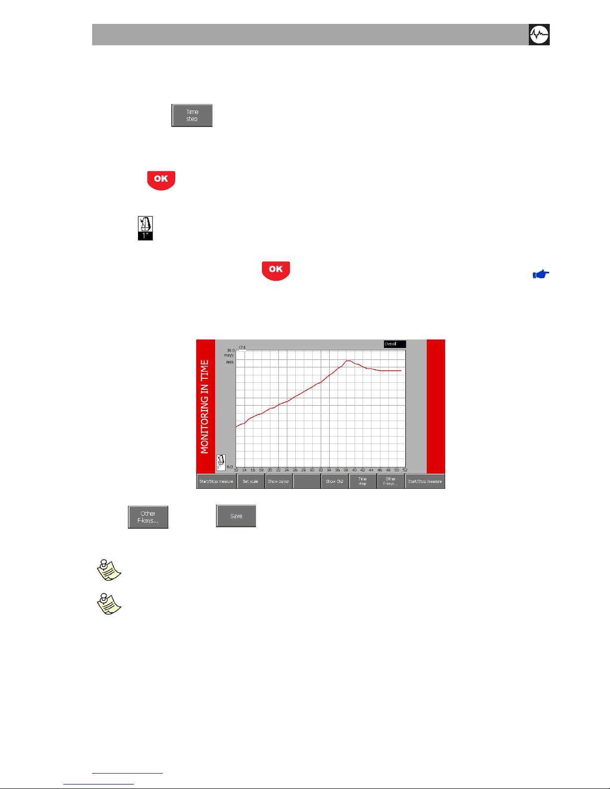
5.2 monItorInG In tIme
The monitoring in time function allows observing (and memorizing if necessary) of the
trend of the overall vibration value plotted against time. For such purpose, it is necessary to preset a value which is adequate
for the parameter F5
by selecting from the following possibilities:
• 1’’ - one second
• 10’’ - ten seconds
• 1’ - one minute
• 15’ - fteen minutes
After pressing
a measurement is made of the overall value, indicated by a point on the graph; such measurement
is automatically repeated according to the preset time step, and a new point is represented in the graph. Availability of a
new measurement is signalled by momentarily displaying the time step in white on black background (under the icon with
metronome
).
When the number of measurements made exceeds forty, just the most recent forty measurements are shown in the graph.
Monitoring is stopped by a further pressing of
and the typical control functions of the graphs become available (
FUNCTIONS OPERATING ON THE GRAPHS).
• Set scale (with which it is also possible display all the measurements made)
• Show cursor
• Change of channel displayed
• List of peaks
When F6
and then F4 is selected, the entire monitoring can be saved in a le for subsequent analysis.
When the acquisition is enabled for both channels, the data save is performed automatically for both channels in the same
le.
as access to the monitoring in time Function is gained From the vibrometer screen, the settings used For cal-
culation oF the overall value are the ones selected in the vibrometer setup screen.
the memory allotted For a single monitoring, allows memorizing a maximum oF 1024 values per channel: when the
limit is reached, the acquisition is stopped automatically without data loss. For this reason, it is important to use
the most suitable Frequency according to the duration oF the phenomenon concerned.
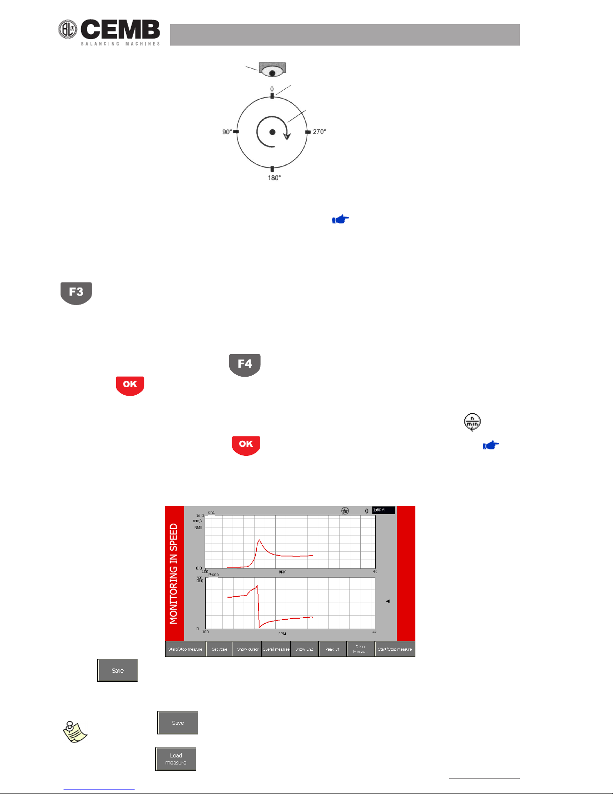
5.3 monItorInG In speed
In many situations it could prove useful to associate the vibration value with that of the speed of rotation of a shaft; in this
way it could be possible to investigate, for example, how the overall or the synchronous component varies during machine
starting or stop phase, with identication of any critical zones or zones with risk of resonance, which are best to avoid.
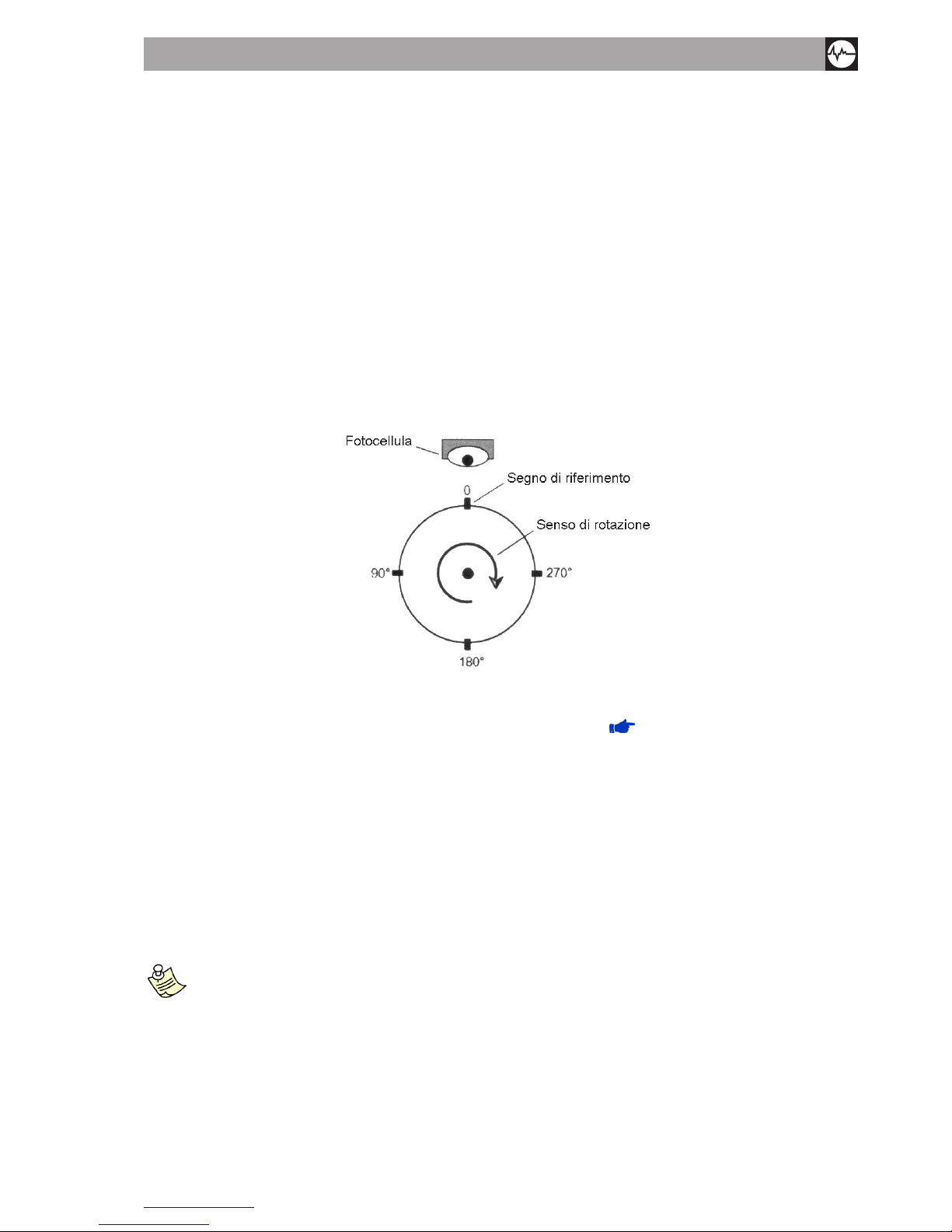
In order to be able to use this function, it is essential to have the tachometric signal; therefore it is necessary:
• to apply a reecting label on the rotor as reference mark (0°). Starting from this position, proceed to measure the angles
in direction opposite to that of the shaft rotation.
24
N600 - Ver. 2.2 09/2015
photocell
reference MarK
rotation SenSe
• connect the photocell and position it correctly (50 - 400 mm), so that the led located behind it lights up once for each rev.
when the reference mark is illuminated by the light beam. If the operation is not regular, either retract or approach the
photocell, or else incline it with the respect to the workpiece surface. APPENDIX D - LASER SENSOR FOR CEMB
N INSTRUMENTS.
Speed monitoring can be performed according to two different modes, namely:
• monitoring of overall vibration (overall)
• monitoring of modulus and phase of the vibration synchronous with the speed of rotation (1xRPM)
An icon on the top part of the page indicates which mode is currently selected; this mode can be changed by pressing
.
Two graphs are always displayed simultaneously in a synchronous monitoring. Such graphs can be:
• modulus and phase of the vibration of channel 1
• modulus and phase of the vibration of channel 2
• modulus of the vibration for both channels
To switch between the various modes, press
After pressing a vibration measurement is made and a speed reading taken, these are then plotted by a point on
the graph; such measurements are repeated automatically, with a new point added each time to the graph. For the sake of
convenience, the current rotor speed, expressed in RPM, is displayed at the top right, alongside the symbol .
Monitoring is stopped by a further pressing of , and the typical graph control functions become available ( FUN-
CTIONS OPERATING ON THE GRAPHS).
• Set scale
• Show cursor
• Change of channel displayed
• List of peaks
When F4 is pressed, the entire monitoring can be saved in a le for subsequent analysis.
When the acquisition is enabled for both channels, the data save is performed automatically for both channels in the same
le.
the F4 button allows saving the measurements, selecting the appropriate measurement point in the
tree element relating to the currently selected route.
the F2 button allows reloading the measurements previously processed by the instrument.

Vibration equipment division
25
N600 - Ver. 2.2 09/2015
6. FFt (Fast FourIer transForm) analyzer mode
A complete analysis of the vibration cannot fail to take into account the study of the various factors contributing towards
forming its overall value. Hence it is essential to be able to carry out spectrum analysis with FFT (Fast Fourier Transform)
algorithm. Such technique allows splitting and memorizing a measured signal into its component frequencies in a certain
period of time, thus making it easier to discover their causes. Analysis of the highest peaks in the spectrum, together with
analysis of the frequencies to which they correspond allows determining which are the principle sources of vibration and,
therefore, the aspects on which to act in order to reduce them. Although a spectrum contains a series of very signicant
information, its interpretation requires a certain amount of experience and attention; for this purpose, the material given in
APPENDIX C - A RAPID GUIDE TO INTERPRETING A SPECTRUM COULD BE USEFUL.
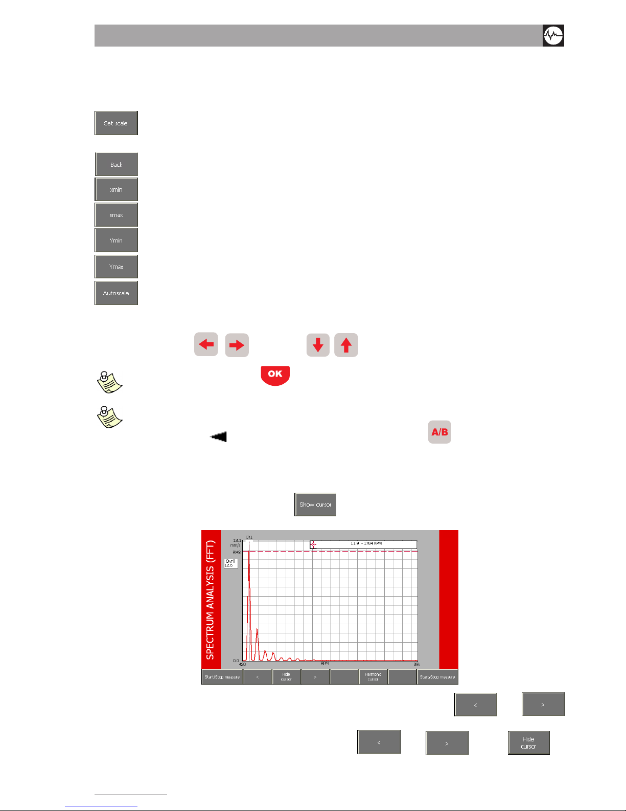
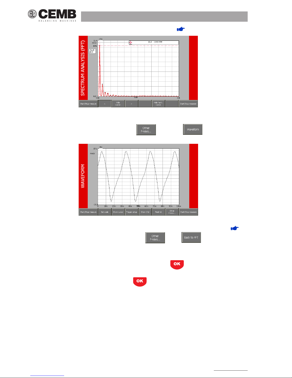
6.1 spectrum analysIs (FFt)
The so-called FFT algorithm is applied to the signals acquired with due respect for the settings made; in accordance with the
recommendations deriving from the mathematical treatment from which it has been taken, such numeric processing is preceded by application of a Hanning window to the acquired signal. This allows attenuating the edge effects due to digitizing as
well as reducing phenomena of leakage in the spectrum. The Measurement page appears like the one shown in the gure.
It is organized so as to maximize as much as possible the area dedicated for representation of the FFT graph.
A box Ovrll is located on the left side giving the overall value of the signal for the channel displayed; it has the same units
of measurement as those of the FFT. Such information allows monitoring the total vibration, also during the analysis of its
single components.
Beside the usual graphic control functions (
FUNCTIONS OPERATING ON GRAPHS), namely:
• Set scale
• Show cursor
• Change of displayed channel
• List of peaks in order to display the list of highest peaks in the spectrum ( LIST OF PEAKS).
the following are available:
• Waveform ( WAVEFORM FUNCTION)
• Trigger Setup to set a trigger to be used for starting the acquisition ( TRIGGER SETUP).
6.2 HarmonIc cursor
When the cursor is displayed on an FFT graph ( USE OF THE CURSOR), it means that a special mode known as harmonic
cursor is available.
The frequency at which the cursor is currently positioned when F5
is pressed, is considered as the fundamental
frequency of the signal under examination, and on the graph all the harmonics of higher order (2nd, 3rd, 4th, …) are marked
Shifting of the cursor, which varies the frequency considered as fundamental, causes the automatic updating of the position
of all the multiple ones.
Use of the harmonic cursor allows easy recognition in the spectrum of families of peaks in correspondence of frequencies,
26
N600 - Ver. 2.2 09/2015
which are multiples between each other, and typically indicative of special defects ( APPENDIX C).
6.3 waVeForm FunctIon
In the second series of functions (accessed by pressing F6 ) is present F1 which allows access to a
page where the vibration signals are shown in relation to time.
In this mode, the N600 instrument can be used as an actual oscilloscope, and further enhances the variety of information
which can be deduced from the vibration signals. This mode also contains all the typical graph control functions ( FUN-
CTIONS OPERATING ON GRAPHS).
It is possible to return to SPECTRUM ANALYSIS by selecting F6 e poi F1 .
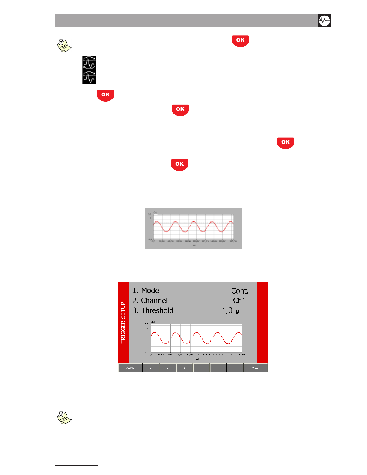
6.4 trIGGer setup
In certain cases, it could be useful for acquisition not to start with the pressing of by the operator, rather with a certain
condition associated with the phenomenon being observed; this is possible by enabling the so-called trigger. In this way, the
measurement does not started immediately after pressing , but only when the signal of the trigger channel exceeds
a preset threshold.
Operation of a trigger can be enabled in two distinct modes, namely:
• Cont. (continuous mode)
• Single (single measurement)
and requires presetting of
• a channel
• a threshold
One of the most frequent uses is the so-called Impact test: A hammer is used to stress a structure and to cause it to vibrate
in order to determine its natural frequencies. For such purpose, a sensor should be placed in the zone to be examined and
a threshold value chosen, which is higher than the background noise read, but lower than that produced by the hammering
with which the structure is stressed.
Vibration equipment division
27
N600 - Ver. 2.2 09/2015
Trigger threshold
aFter enabling the trigger and selecting the required settings, press to return to the measurement page
in which the mode selected For the trigger is speciFied by a speciFic icon:
-
continuous mode
-
“single measurement” mode
Now merely press , and wait for the trigger threshold to be exceeded. If it is required to stop the procedure manually
(before or after exceeding the threshold), just press again.
6.4.1 modes
This is the parameter which indicates whether the trigger is:
• OFF (disabled): the measurement is started and stopped manually by the operator on pressing
• Cont. (enabled in continuous mode): acquisition is started when the signal exceeds the trigger threshold, and continues
until the operator stops it manually (by pressing )
• Single (enabled in “single measurement” mode): when the signal exceeds the trigger threshold, a single measurement
is made (duly observing the parameters set for the FFT), then the acquisition is stopped automatically; this is the most
frequently used mode because it allows analyzing phenomena of transitory type; by suitably presetting the FFT parame-
ters, it is possible to obtain an acquisition time sufciently long for containing all the important information.
Subsequent acquisitions would only succeed in capturing noise, therefore they would be counter-productive.
When the trigger is enabled, the following settings become visible in the TRIGGER SETUP page:
• Channel
• Threshold
6.4.2 channel
This indicates on which channel (Ch1 or Ch2) to make the comparison between the signal value and the threshold value in
order to activate the acquisition.
iF just one oF the two measuring channels is enabled, obviously choice oF the trigger channel is obligatory, hence
it is Forced automatically.
28
N600 - Ver. 2.2 09/2015
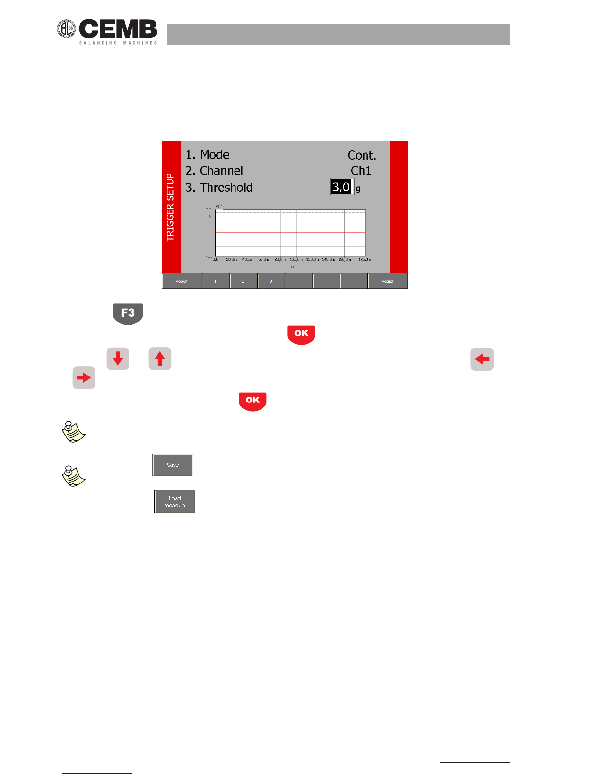
6.4.3 threshold
This is the level which the signal must exceed (in a leading edge of the waveform) in order for the acquisition to be started
automatically. The selection of a suitable value is normally one of the most delicate operations, but by using the N600 instru-
ment it is considerably simplied. The graph at the bottom of the page shows in real time the signal of the trigger channel (in
continuous line) and the current threshold (broken line). Hence the effect of different values can be assessed immediately,
thus making it easier to make a rapid choice of the value considered most appropriate.
After pressing the threshold value can be preset in two ways, namely:
• by typing, using the numeric keyboard (only after pressing , it is possible to shift the broken line in the graph);
• by using and , to increase or decrease the value of a single digit, which can be selected with and
(the broken line in the graph is shifted
• immediately, however at the end, pressing of is always necessary in order to conrm).
the trigger threshold should always be set in the unit oF natural measurement oF the sensor. however, in the
measurement page, it is possible to supply the vibration in other units even iF this is not recommended when making
measurements with the trigger enabled.
the F5 button allows saving the measurements, selecting the appropriate measurement point in the
tree element relating to the currently selected route.
the F2 button allows reloading the measurements previously processed by the instrument.
Vibration equipment division
29
N600 - Ver. 2.2 09/2015
7. balancer mode
One of the causes of vibration most frequently encountered in actual practice, is the unbalance of a rotating part (lack of
uniformity of the mass about its axis of rotation); such unbalance can be corrected with a balancing procedure.
The N600 instrument allows balancing any rotor under service conditions in one or two planes, by using one or two vibration
pick-ups and a photocell.
Ad hoc procedures have been drawn up for the most frequent situations (balancing on one plane with just one sensor and
balancing on two planes with two sensors). These procedures guide the operator step-by-step through the sequence of
operations. A general guided procedure is available for all the other cases (rarely used).
Some rules to be observed in order to perform correct balancing are as follows:
• place the sensors as close as possible to the supports of the rotor to be balanced, by using the magnetic base or by
fastening via a tapped hole to ensure good repeatability;
• apply a reecting label on the rotor as reference mark (0°). The angles are measured, starting from this position, in direc-
tion opposite to that of shaft rotation.
• connect the photocell and place it in correct position (50 – 400 mm), so that the led at the back of the photocell lights up
only just once per rev. when the light beam illuminates the reference mark. If operation is incorrect, either retract or approach the photocell or else incline it with respect to the workpiece surface. ( APPENDIX D - Laser sensor for CEMB
N instruments).
For further consideration, see attached brochure BALANCING ACCURACY FOR RIGID ROTORS.
The balancing procedure consists of two parts, namely:
• calibration: a series of spins allows determining the parameters required for balancing in the case of a given rotor
• measurement of the unbalance and calculation of the correction.
As the calibration is normally a laborious procedure, the parameters derived should be memorized, then called in the case
of subsequent maintenance work on the same machine. This is possible via the balancing programs: a program is dened
with a series of settings in order to work on a particular rotor and it contains all the information and data acquired regarding
such rotor. It is possible to save the current program at any moment in a special archive so that it is available at later dates.
iF it is required to use data and parameters oF a previously stored program, it is essential to mount the transducer
in exactly the same position on the rotor..

30
N600 - Ver. 2.2 09/2015
7.1 selectIon oF tHe balancInG proGram
When the balancing function is selected, a page is presented to the operator in which to select the balancing program to be
used, choosing between the following options:
• new program
• loading of program from archive
• use of current program (only available if a program has been previously created or loaded)
• copy archive to USB key
7.1.1 new program - Balancing setup
The creation of a new program entails setting of a series of parameters. This is done in the BALANCING SETUP screen.
7.1.1.1 numBer oF planes
This is the number of planes on which to act to correct the unbalance of the rotor. The number can be 1 or 2..
7.1.1.2 Filter accuracy
Balancing under not particularly stable signal conditions is certainly critical and needs acquisition for longer times in order to
obtain a satisfactory quality of the value measured. This can be achieved by acting on the lter accuracy:
acquisition made with a broad lter: faster, but only suitable for particularly stable signal conditions (high
unbalance values)
acquisition made with a narrow lter: suitable in most conditions
acquisition made with a very narrow lter: suitable for particularly critical signal conditions (low unbalan-
ce values); requires longer times
Vibration equipment division
31
N600 - Ver. 2.2 09/2015
depending on the accuracy selected For the Filter, the instrument automatically determines the number oF revs. ne
cessary For each acquisition. as it could be necessary to have up to some hundred revs. in certain situations, the
time required For each measurement could likewise be equal to some tens oF a second. taking into account that a
certain number oF consecutive acquisitions is necessary so that the quality oF the measurement can reach accepta-
ble levels, the time required For an acquisition could also entail several minutes in the case oF slow rotors. For
example, For a rotor with speed oF rotation 600 rpm, it could be necessary to wait up to 10 seconds beFore being
able to view the First result oF the measurement.
Conrmation of the settings made (with ) creates a new balancing program not associated with any name, seeing as
though it is directly accessible as current program. Only when saving in the archive, will there be a request to the operator
to enter a special name which will characterize it from that moment on.
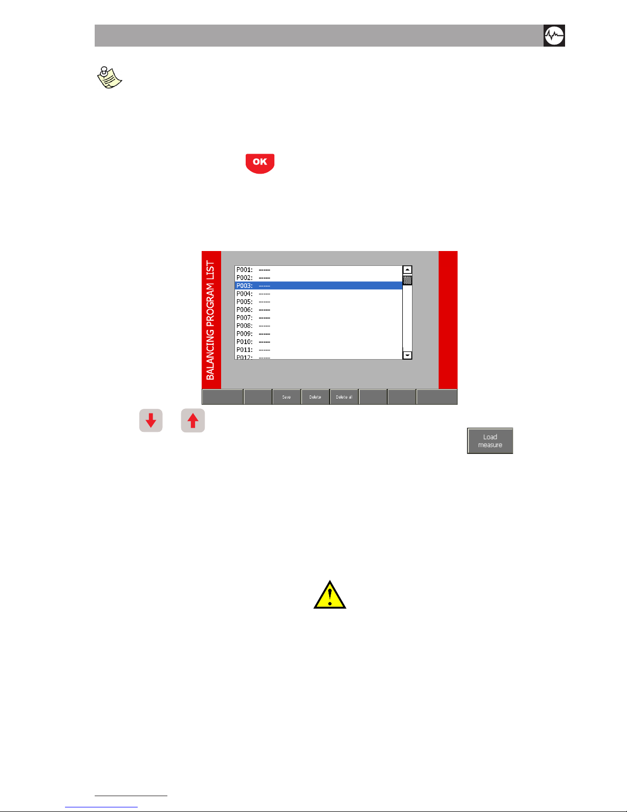
7.1.2 load program From archive
When this option is selected, access is gained to the program archive.
Arrow keys and allows scrolling the 10 available positions, thus selecting the required program (visible in nega-
tive, i.e. with white writing on black background); the program can then be loaded by pressing F1 .
If it is not possible to carry out the operation correctly (e.g. attempt made to load a program from an empty position, indicated
by the symbol -----), an error message appears in the black band in the bottom area of the page.
After loading, the following is displayed:
• the measurement and unbalance correction screen, if the calibration procedure has already been completed
• the calibration screen, if not.
7.1.3 use current program
This option allows resuming the last program used (new or loaded), exactly from the point where it had been abandoned.
————————————————————————————————————————————————————
warnInG!
wHen tHe Instrument Is swItcHed oFF, tHIs causes loss oF unsaVed data (and tHereFore oF tHe current proGram); Hence tHIs
optIon Is not InItIally aVaIlable wHen tHe Instrument Is swItcHed on aGaIn; It becomes aVaIlable only aFter
a proGram Has been created or loaded From tHe arcHIVe.
————————————————————————————————————————————————————
7.1.4
copy archive to usB key
Allows to export on a USB key connected to the instrument all balancing programs previously saved.
It will create a le “Unb_Data.ini”, necessary to do custom balancing reports (using N-Pro software).

32
N600 - Ver. 2.2 09/2015
2
1
3
4
7
9
5
6
8
10
1
5
2
3
4
7
9
6
8
10
7.2 calIbratIon sequence
The calibration operation, necessary for assessing the unbalance of a rotor, is normally a procedure consisting of various
steps. Above all, for the most common two cases, it consists of:
• Calibration for balancing on one plane:
> rst spin without test weight
> second spin with test weight on the balancing plane
• Calibration for balancing on two planes:
> rst spin without test weight
> second spin with test weight only on the rst balancing plane
> third spin with test weight only on the second balancing plane
For the two congurations:
• correction on one plane with one sensor
• correction on two planes with two sensors
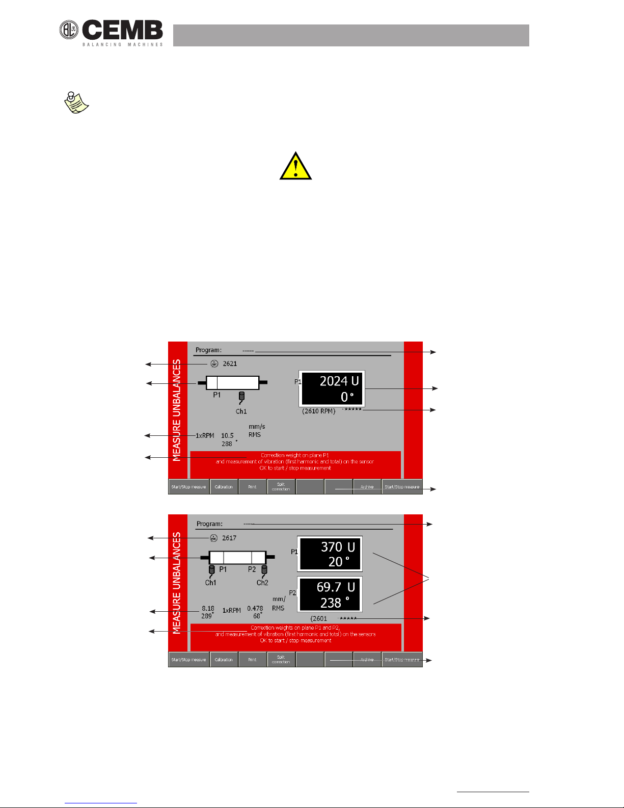
The calibration sequence screen on the N600 instrument is organized as in the gures:
1. number and name of the balancing program (if loaded from the archive), or else ----
2. current speed of rotation, in RPM
3. ayout of the position of the sensors and correction planes on the rotor; indication of the plane on which to apply the test
weight
this representation is approximate only; the sensors and correction planes can be chosen in any position relative
to each other (external sensors or sensors inside planes, ... ) since the calibration serves especially For determi-
ning correctparameters For balancing in any conFiguration.
4. value and angular position of any test weight
5. indication of the vibration component synchronous with the rotation (unbalance) in value and phase for every measuring
channel
6. average speed of rotation and lter accuracy with which the vibration has been measured

Vibration equipment division
33
N600 - Ver. 2.2 09/2015
the average speed value is highly important because the calibration procedure can only be considered as properly
perFormed iF between one step and the other, such speed does not exhibit diFFerences exceeding 5%. it is up to the
operator to check For this condition.
7. indication of the number of calibration step selected
8. indication of the status of the calibration steps
> completed
> to be done
9. instructions for the current calibration step
10. functions for selecting the calibration step
(F1): go the previous step
(F6): go to next step (if the current step is the last step of the sequence, this function, which is indicated by
F6 , ends the calibration and loads the unbalance measuring page)
when each already completed step is selected, the available data appear on the monitor (vibration, average measu-
ring speed, ... ). such inFormation is useFul, also at a later date, to decide whether to repeat or not to repeat the
measurement.
although it is advisable to perForm the calibration steps in the order in which they appear, it is perFectly possible
to select a diFFerent order according to your particular requirements.
7.3 executIon oF measurement
To start the measurement in any of these steps, press ; a pop-up panel appears showing, in real time, the quality of
the current measurement (for each channel).
The higher is the level of the bars, the better will be the quality of the measurement (which is averaged over time). After
reaching the required level, stop the measurement again by pressing
.
If the operator decides to accept the value, then he must press
corresponding to the option , which
ashes in order to warn the operator the importance of pressing it.
When the measurement is accepted, the corresponding calibration step is indicated as complete
.
unstable signals produce measurements whose quality is unable to reach acceptable levels; under these conditions, it
is advisable to increase Filter accuracy (
Filter accuracy) and consequently repeat the entire procedure.
iF the quality oF a particular measurement has been altered by a special event (e.g. an impact), the time required
to go back to it could be excessively long; to speed it up, the measurement can be reset manually by pressing
.
7.3.1 test weight
Calibration requires the use of a test weight, to be applied in succession on the various correction planes. These two para-
meters should be preset, with the appropriate functions F2
and F3 by typing the appropriate values
with the numeric keypad, and conrming with
.
34
N600 - Ver. 2.2 09/2015
2
1
3
6
7
5
8
1
4
2
3
6
7
5
8
4
To cover the various operational requirements when balancing on two planes, it is possible to specify a different test weight
(value and angular position) on plane 1 and on plane 2.
the value oF the test weight should be indicated in general units u. the operator can decide independently to make
these u correspond to the physical units preFerred by him, bearing in mind that also the unbalance and necessary
correction will be indicated in the same units u.
————————————————————————————————————————————————————
warnInG!
correct cHoIce Has been made oF tHe test weIGHt IF It produces, In eacH oF tHe spIns, a suFFIcIent VarIatIon In tHe VIbratIon
compared to tHat oF tHe InItIal spIn.
tHIs may be consIdered satIsFactory IF we HaVe at least one From tHe FollowInG:
- VarIatIon In module oF at least 30%
- VarIatIon In pHase oF at least 30°
————————————————————————————————————————————————————
7.4 unbalance measurement and calculatIon oF tHe correctIon
In appearance the UNBALANCE MEASUREMENT page is very similar to the calibration page:
and the following information is given:
1. number and name of the balancing program (when loaded from the archive), otherwise ----
2. current speed of rotation, in RPM
3. layout of the position of the sensors and correction planes on the rotor
Vibration equipment division
35
N600 - Ver. 2.2 09/2015
this representation is approximate only; the sensors and correction planes can be chosen in any position relative
to each other (external sensors or sensors inside the planes, ... ) since the calibration serves especially For de-
termining correct parameters For balancing in any conFiguration.
4. indication of the correction weight, in value and position on every plane
the module is indicated in general units u, corresponding to those used in setting the test weight. as the program
makes use oF correction through addition oF material, the position indicated is the one where to add the correc-
tion weight. when it is required to proceed by removal oF material, act in a position diametrically opposite (add
180° to the displayed phase)
5. average speed of rotation and lter accuracy with which the unbalance has been measured
————————————————————————————————————————————————————
warnInG!
tHe aVeraGe speed Value Is Important because It allows cHeckInG wHetHer tHe measurement Has been made at a speed not
too dIFFerent From tHat used In tHe calIbratIon spIns (dIFFerences less tHan 5%). owInG to small amounts oF non
lInearIty always preset In actual practIce, It Is not adVIsable to proceed to calculate tHe correctIon at a speed too wIdely
dIFFerent From tHe calIbratIon speed. cHeckInG oF tHIs condItIon Is up to tHe operator.
————————————————————————————————————————————————————
6. value and phase of the vibration synchronous with the rotation (1xRPM) and total value(Overall) vibration measured via
the sensors
this inFormation is considerably important as indicator oF the reliability oF the balancing: what concerns us in
actual practice is to reduce the vibration to under a certain value considered as tolerable ( appendix B
).
however reduction oF the unbalance only has eFFect on the 1xrpm component. a low value oF this component,
accompanied by a high overall indicates problems diFFering From those oF unbalance, which, thereFore, cannot be
corrected by balancing.
7. instructions for unbalance measurement and calculation of the correction
8. functions available
(F1): calibration procedure
iF the calibration procedure has not been completed, this button starts Flashing, to warn the operator to return
to the calibration procedure beFore being able to make unbalance measurements. iF not, indication is already given
oF the correction weights and positions where to act, deduced From the calibration spins.
(F2): direct printing of a balancing certicate by using the portable printer provided (optional). The certicate
gives the unbalances on the correction planes (in units U), as well as the values of vibration (overall and
synchronous) of these planes.
(F3): function involving splitting of the correction weight on two presettable angles ( SPLITTING OF COR-
RECTION WEIGHT).
(F6): shows the program archive (to allow saving or eliminating a program).
As in calibration, to start or stop measurement, press ; while the measurement is active a pop-up appears to indicate
the quality of measurement of each channel. After making the corrections indicated, the measurement-correction procedure
can be repeated until the required conditions are met (typically vibration measured by the sensors lower than a certain value).
36
N600 - Ver. 2.2 09/2015
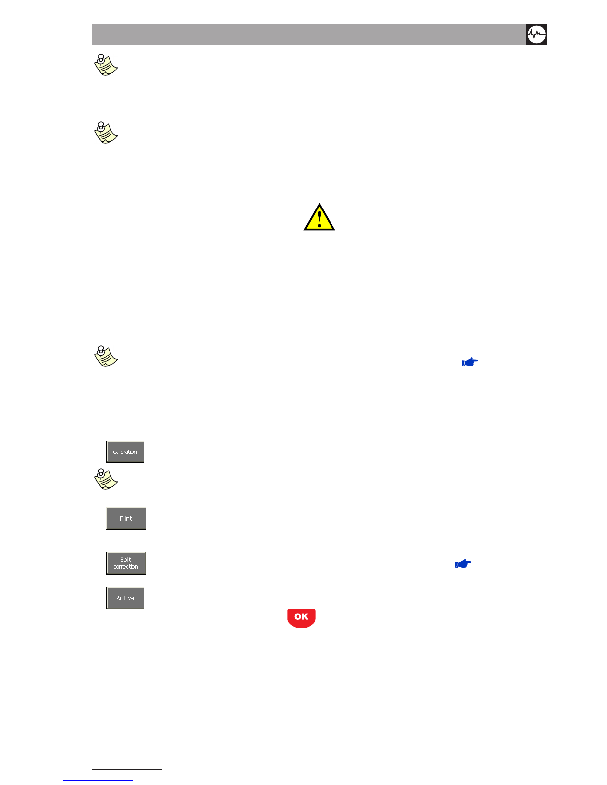
7.5 splIttInG oF correctIon weIGHt
In this page it is possible to select between the correction modes:
• by addition of material
• by removal of material
•
by pressing push buttons F1 and respectively.
In certain practical situations it is not possible to correct in the position calculated theoretically as optimum position: in the
case of a fan, for example, such position could fall in the gap between two blades, where obviously it is not possible to add
or remove material. However, it is often the case also for uniform rotors, to prefer to correct where holes are already present,
or else to avoid acting in particular zones.
The split function of the N600 function calculates the weights to be applied or to remove corresponding to any two positions
α1 and α2, so that their effects are equivalent to those of the correction calculated by the balancing algorithm.
When F3
or F4 is pressed, the user can assign the most appropriate value to these two positions,
by selecting from those effectively available in practice for that particular rotor. By pressing
the two corresponding
correction weights are automatically calculated and displayed.
Such operation can be performed separately on each of the planes, after selecting the required one by pressing
.
Pressing F6 you go back to the residual unbalance page.
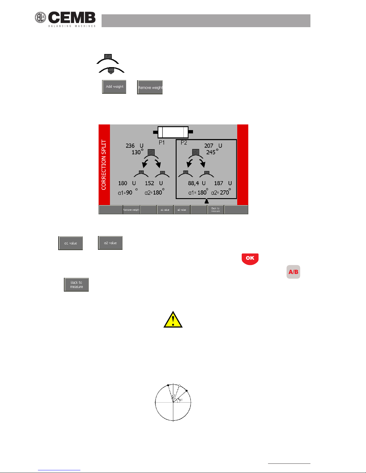
————————————————————————————————————————————————————
warnInG!
wHateVer tHe Value oF α1 and α2, tHe anGle oF reVolutIon Is subdIVIded Into two parts, one part
conVex (<180°) and tHe otHer concaVe (>180°).
In order to carry out tHe splIttInG, anGles α1 and α2 sHould be cHosen so tHat tHe correctIon posItIon
calculated durInG balancInG, lIes wItHIn tHe conVex zone.
IF not, sucH splIttInG would be ImpossIble, and tHe n600 Instrument would IndIcate zero as correctIon
weIGHt For botH posItIons
α
1 and
α2.
————————————————————————————————————————————————————

Vibration equipment division
37
N600 - Ver. 2.2 09/2015
it is useFul to observe that the more the α1 and α2 positions are Further apart From the position calculated in
balancing, the higher must be the values oF the corresponding weights. hence it is advisable to select α1 and α2 as
close as possible to the correction angle obtained by the balancing operation, or at least to make sure that they
diFFer by less than 150°.
7.6 saVInG oF a balancInG proGram
After displaying the program archive, proceed to select (with and the position in which to save the current program.
When F2 is pressed, a pop-up appears in which to enter the program name, as explained in ALPHANUMERIC
KEYPAD.
Instead, when F3 is pressed, the selected program can be eliminated, provided it is not the current one.
With F4 it is possible to eliminate all the balancing programs contained in the archive.

38
N600 - Ver. 2.2 09/2015
8. data manaGer mode
The N600 instrument operates following a route logic in which all the data processed and collected by the measuring instrument can be saved.
These routes are divided into two distinct types:
• Soft Route (can be created with the RouteManager software). You can create a “simplied” route directly on the instru-
ment - NEW PROJECT.
It is characterised by the fact that two measurement points are created, whose measurement setup can be modied at
any time.
• Strict Route (can only be created with RouteManager). It is characterised by the fact that the measurement points crea-
ted have a measurement setup set via software and is hence not modiable during data acquisition.
When pressing a PROJECT MANAGEMENT screen appears in which you can select from the following options:
• Open existing project (select the available projects from a list)
• Change selected points (select a measurement point in the tree element of the project selected)
• New project (create a new Soft Route)
• Import projects from USB key (import a Soft/Strict Route created via software and previously saved to USB key)
• Export projects to USB key (export a route from the instrument to USB key)
• Delete projects (delete an existing project from the instrument).
8.1 open exIstInG project
The projects (routes) saved on the N600 instrument can be selected via this function. To change the active project, scroll
through the list using the arrows and ; and select the project involved (recognisable by white text on a blue
background) and conrm by pressing F1 .

Vibration equipment division
39
N600 - Ver. 2.2 09/2015
If you select a Strict Route, the PROJECT STRUCTURE screen will appear; scroll through the list of measurement points
using the arrows
and and select the rst point in the list by pressing F2 .
The measurement acquired will be set according to the settings made during route creation; the measurement functions
(vibrometer, FFT, waveform, monitor_T and monitor_V) will be characterised by the logo
, and the name of the mea-
surement point will be shown at the top of the graph.
in the case oF analysis using a strict route, this measurement setup Function allows checking but not modiFying
the parameters set.
T
he symbol allows identiFying a setup relating to a strict route.
iF you select a soFt route, a pop-up will appear inForming you oF the route type selected and the procedure to
save the acquired data.
press to conFirm the above pop-up.
8.2 cHanGe selected poInts
If a Strict Route is active, this function can be used to change the points of the tree element related to the selected route. For
each measurement point selected, the measurement will be acquired according to the settings made during route creation
via the RouteManager software.
Accessing this function, you can view the PROJECT STRUCTURE screen relating to the tree corresponding to the currently
active route. Use the arrows
and to select the measurement point involved and press F5 to conrm
the measurement point.
in case oF analysis with soFt route active, accessing this Function, a pop-up inForms you that the measurement
points to which to attribute/save the reading are to be selected at the time oF saving the measurement. pressing
,
you go back to the initial screen.
40
N600 - Ver. 2.2 09/2015
8.3 new project
This function allows creating a Soft Route directly on the N600 instrument characterised by only two measurement points.
A pop-up window will appear in which to enter the desired name, as explained in ALPHANUMERICAL KEYPAD.
Type in the desired name and conrm by pressing . At this point, the Soft Route previously created will automatically
be activated.
8.4 Import projects From
USB
key
This function allows copying all the projects saved on the USB key inserted in the N600 instrument to its internal memory. A
pop-up will inform you when the operation has successfully been completed. Conrm by pressing .
As the instrument is characterised by a Windows-based operating system, any USB key formatted with this system can be
connected to the instrument.
————————————————————————————————————————————————————
cautIon!
IF you access tHIs FunctIon wItHout HaVInG FIrst Inserted a usb key In tHe dedIcated port,
a pop-up wIll InForm you to Insert It.
————————————————————————————————————————————————————
8.5 export projects to usb key
This function allows exporting the routes saved on the N600 instrument to a USB key. Accessing this function via ,
the Project List page appears. Scroll through the list using the arrows and and select the route you want to copy
to USB key (white text on blue background). Conrm by pressing F2 , A pop-up will inform you when the operation
has successfully been completed. Close the pop-up by pressing .

Vibration equipment division
41
N600 - Ver. 2.2 09/2015
iF you want to copy a project already saved to the
USB
key, a pop-up will ask you to conFirm that you want to
overwrite the File.
iF you access this Function without having inserted a
USB
key in the dedicated port, a pop-up will ask you to insert
it.
8.6 delete projects
This function allows deleting projects saved in the instrument. To delete a single project, press F5 , scroll through
the Project List using the arrows
and and select the project you want to delete.
You can delete all the projects saved in the instrument by pressing F6
.
you cannot delete the currently active project From the list.

42
N600 - Ver. 2.2 09/2015
9. arcHIVe FunctIon
The N600 instrument allows viewing and managing screenshots previously stored by pressing , using this specic
function directly accessible from the start screen.
Pressing F6 an ARCHIVE screen is shown where you can select from two options:
• load screenshot (view previously stored screenshots)
• delete screenshots (delete one or all the stored screenshots).
9.1 load screensHot
You can load and view the previously stored screenshots on the display.
The page shows as a list of positions where the screenshots are stored:
Select the screenshot to be loaded using the arrows
and ; then press F1 to load the screenshot
selected.
Vibration equipment division
43
N600 - Ver. 2.2 09/2015
To go back to the list of stored screenshots, press or to go back to the main screen.
the screenshots loaded will be characterised by the icon , to indicate that you are not viewing data but a
screenshot acquired previously.
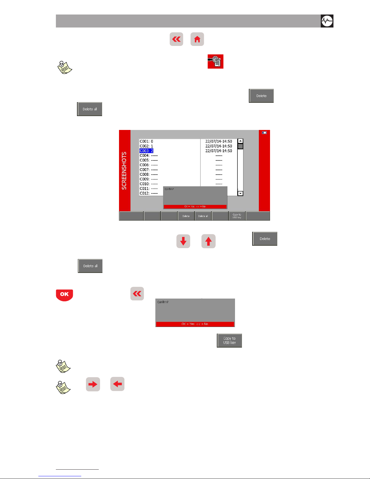
9.2 delete screensHots
To delete a screenshot and clear the corresponding position in the archive, press F3 .To delete all screenshots,
press F4
.
The page shows a list of positions where the screenshots are stored.
Select the screenshot to be deleted using the arrows
and ; then press F3 to delete the screenshot
selected.
Press F4
, to delete all the screenshots at the same time.
When pressing the above mentioned buttons, the popup shown below asks you to conrm the operation with the button
or to quit with the button .
For the functions “Load screenshot” and “Delete screenshots”, press F6
to copy all the screenshots stored on the
instrument to a Screenshots folder that will automatically be created on the USB key inserted in the instrument.
each time you want to save new screenshots to the same usb key, new subFolders will be created in the
screenshots Folder named with the date and time.
the and , buttons, which respectively increase and decrease the position selected by 10 can be used to
quickly scroll through the archive.
44
N600 - Ver. 2.2 09/2015
10. CEMB N-Pro PrograM (oPtioNal)
Data saved in the N100, N300 and N600 instruments can easily be imported into a PC, organised and saved to the hard disk
and subsequently analysed, compared, printed, etc.
These operations are made possible thanks to CEMB N-Pro software (Professional Environment for N-Instruments), available for Microsoft Windows operating systems. The interface has been carefully designed to make it intuitive and therefore
extremely simple to use even for inexperienced users.
This chapTe r refers To The “N iNsTrumeNT” or “N apparaTus”, geNe ric expressioNs ThaT refer exclus ively To The
N100, N300 aNd N600 models wiTh which cemB N-pro sofTware caN Be used (commuNicaTioN, daTa orgaNisaTioN,
priNTiNg, eTc...).
N-pro sofTware caNNoT Be used wiTh oTher cemB iNsTrumeNTs, iNcludiNg Those from The N raNge.
10.1 SyStEM rEquirEMENtS
Installation and use of the CEMB N-Pro program requires:
• a processor: at least Intel Pentium IV 1GHz, or Athlon equivalent
• memory: 512MB (recommended: 1GB or more)
• space on disk: at least 400MB free before installation (excluding space subsequently required for the data records)
• operating system:
> Microsoft Windows 2000 almeno Service Pack 4
> Microsoft Windows XP almeno Service Pack 2
> Microsoft Windows Vista
> Microsoft Windows 7 (32 e 64 bit)
> Microsoft Windows 8 and 8.1 (32 e 64 bit)
• video resolution 1024x768 or better.
10.2 iNStallatioN of thE SoftwarE
Installation of the CEMB N-Pro software must be carried out by launching the setup.exe program, contained in the CD-ROM,
and then clicking on the key without changing any options.
That way the software will be installed in the program directory.
————————————————————————————————————————————————————
warNiNg!
(oNly for N100 aNd N300 iNStruMENtS):
duriNg iNStallatioN of thE SoftwarE a filE will BE CrEatEd CoNtaiNiNg thE drivErS for uSB CoMMuNiCatioN;
it iS thErEforE iMPortaNt that thE CEMB N-Pro SoftwarE iS iNStallEd BEforE thE N100 or N300 iNStruMENt
iS CoNNECtEd to thE PC, othErwiSE MalfuNCtioNiNg May oCCur.
————————————————————————————————————————————————————
wheN updaTiNg from a versioN previous To versioN 1.3.3 iN a wiNdows visTa, wiNdows 7 aNd wiNdows 8 operaTiNg
sysTem, The followiNg operaTioNs musT Be compleTed Before The sofTware caN Be used:
- righT-click oN The cemB N-pro program icoN oN The deskTop
- selecT The ‘compaTiBiliTy’ meNu
- check ThaT The opTioN ‘execuTe program iN operaTiNg mode for’ : has BeeN disaBled
- check ThaT The opTioN ‘execuTe program as admiNisTraTor’ has BeeN disaBled
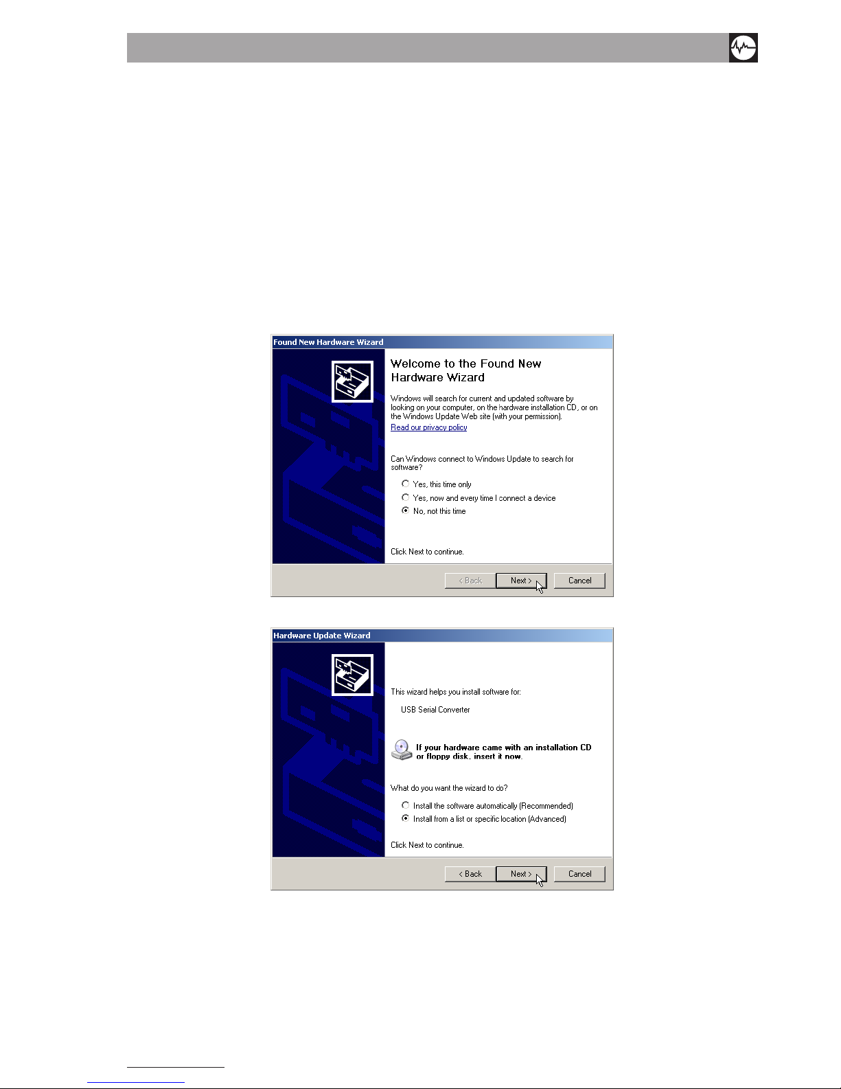
Vibration equipment division
45
N600 - Ver. 2.2 09/2015
- press ok.
10.3 iNStallatioN of drivErS for uSB CoMMuNiCatioN with thE N100, N300 iNStruMENtS (for vErSioN
1.3.4 or EarliEr)
Do not connect the N instrument to the PC using the USB cable supplied until the CEMB N-Pro software has been correctly
installed; after a few seconds the following message will appear:
New hardware found
USB <-> Serial
in the Windows application bar (lower right hand corner).
The add new hardware window will then appear with the guided procedure.
• When requested to authorise Windows to connect to Internet to search for the drivers
• select the option ‘No, not this time’ and press ‘Next>’
• Then select ‘Install from a specic location (Advanced)’ and press ‘Next’ > again
• Enable the options ‘Search for the best driver in these paths’ and ‘Include this path in the search’.
• Using the ‘Search’ button, select the ‘USB driver’ sub-folder from the one in which the CEMB N-Pro software is instal-
led. At this point press ‘Next’ >
At the end of this guided procedure, the ‘USB Serial Converter’ hardware should be correctly installed.
Wait until the Windows application bar displays a new message:
New hardware found
USB Serial Porte
and a second Found New Hardware guided procedure window appears.
Repeat exactly the same steps to install the ‘USB Serial Converter’ hardware.

46
N600 - Ver. 2.2 09/2015
Correct communication between the PC and the N100, N300, N600 instruments is now possible.
To iNsTall The sofTware aNd drivers correcTly you musT have admiNisTraTor righTs oN The pc used; This is possiBle
wheN you logiN as The admiNisTraTor.
10.4 iNStallatioN of drivErS for uSB CoMMuNiCatioN with thE N100 aNd N300 iNStruMENtS (for
vErSioN 1.3.5 aNd latEr oNly)
As of version 1.3.5, the USB drivers for communication with the instruments N100 and N300 are automatically installed with
the N-Pro program.
When the program has been installed, the window “FTDIChip CDM Drivers” for USB driver installation is displayed.
Click Extract:
When done, the window “Welcome to the Device Driver Installation Wizard!” is automatically displayed.
Click Next:
If installation was successful, the following message is displayed:

Vibration equipment division
47
N600 - Ver. 2.2 09/2015
10.5 actIVatInG tHe soFtware
The rst time the software is started a pop-up is displayed containing the software’s serial
number (S/N) and requesting the corresponding activation code.
This can be obtained by sending an e-mail to CEMB customer service Vibration Analysis division (www.cemb.com)
specifying the subject: “CEMB N-Pro activation code” and specifying in the message your data and the serial number (S/N)
as shown in the pop-up.
CEMB customer service will reply by e-mail containing the corresponding activation code (AC).
The same must be entered to complete the procedure for registration and allow the use of the software.
————————————————————————————————————————————————————
warnInG!
to successFully complete reGIstratIon oF tHe cemb n-pro soFtware, It must be opened by a person wItH admInIstrator
rIGHts on tHe pc. tHe proGram can tHen be opened and used by users wItH more lImIted rIGHts
————————————————————————————————————————————————————
selecting “register later” means the soFtware can be used temporarily whilst waiting to receive the activation
code From the cemb customer service
————————————————————————————————————————————————————
warnInG!
InstallatIon oF tHe cemb n-pro soFtware requIres a dIFFerent actIVatIon code For eVery pc, eacH one oF wHIcH requested
must be From cemb In accordance wItH tHe procedure descrIbed aboVe.
————————————————————————————————————————————————————

48
N600 - Ver. 2.2 09/2015
10.6 use oF tHe soFtware
The buttons on the function bar in the upper part of the page allow full access to all of the functions available in the CEMB
N-Pro software.
The data record contents are always visible on the left, subdivided into:
• vibration measurements (overall, or synchronous)
• balancing operations (only for N300 instrument)
All of the remaining space is reserved for information related to the function enabled at that moment in time, as described
in the following paragraphs.
10.6.1 Function Bar
The buttons are grouped together in the function bar according to type:
• Data storage functions:
creates a new folder
displays the contents of the upper folder
searches in the records
copies the element selected
moves the element selected
pastes the element to be copied or moved in the position displayed
deletes the element selected
renames the element selected
• Record viewing functions:
displays the element selected
edits the notes associated with the element displayed (vibration or balancing measurement). For maximum
exibility, 3 different notes can be associated to each element: users are free to enter the information de
emed appropriate on a case by case basis
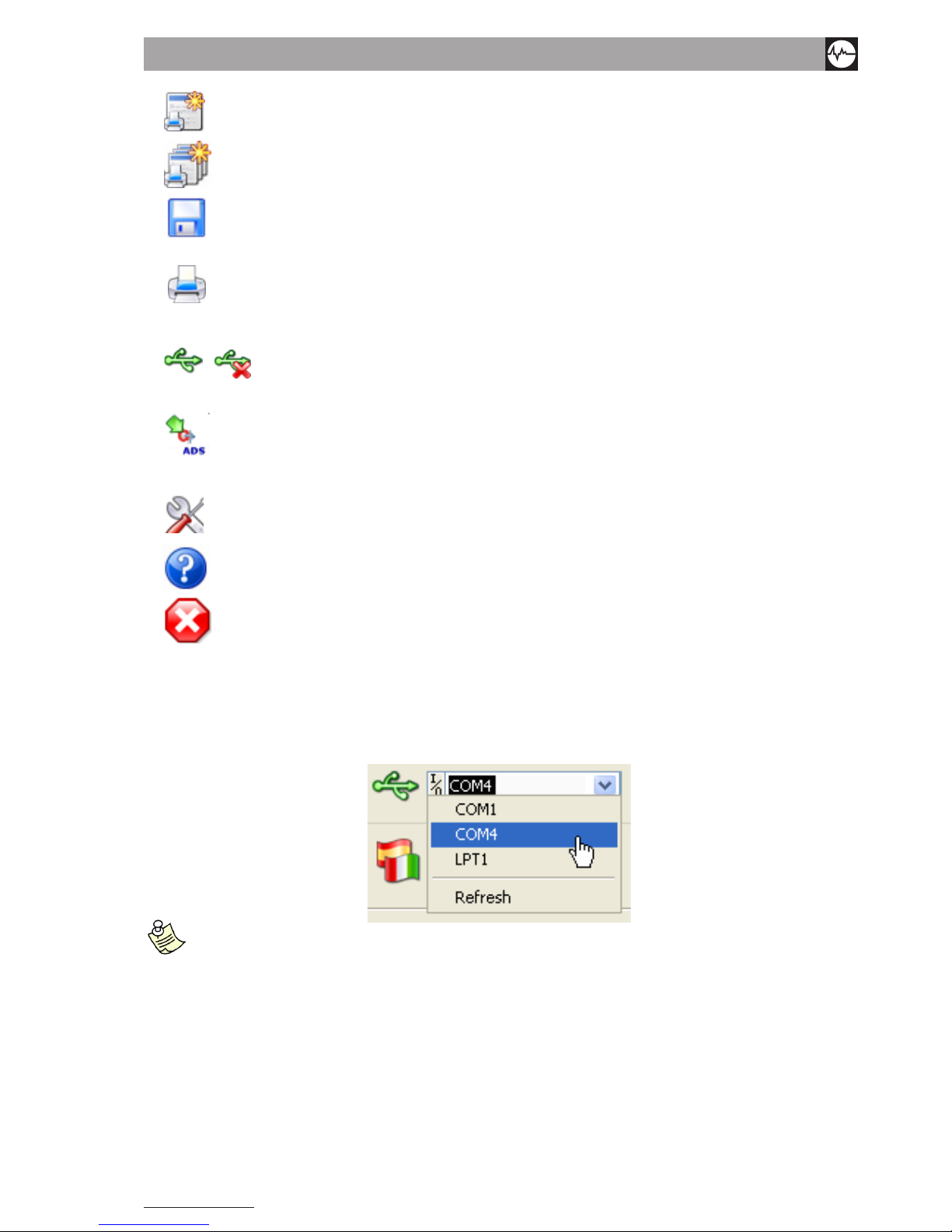
Vibration equipment division
49
N600 - Ver. 2.2 09/2015
generates and displays a report for the element selected
generates and displays a multi-report for the elements selected
saves the report (or multi-report) generated
prints the report (or multi-report) generated
• Function for importing data from the N100 and N300 instruments:
/
starts/quits the automatic procedure for importing data from the N instrument using a USB connection
• Function for importing data from the N600 instrument:
starts the automatic procedure for importing data from the N600 instrument (data previously exported on
USB key
• General functions:
opens the settings window
displays a panel with information related to the software (producer, version, etc...)
quits the program.
10.7 General settInGs
General operating parameters for the CEMB N-Pro software can be set from this window, such as:
• the PC port to which the N instrument will be connected which will be one of the COMx serials available, a list of which
can be displayed by clicking on the drop-down menu (only for N100 and N300 instruments)
to select the port correctly, proceed as Follows:
- with the n instrument (n100 or n300) disconnected From the pc, click on the drop-down menu and select
reFresh, noting the list oF ports available
- connect the n instrument (n100 or n300) to the pc and wait For a Few seconds
- click on the drop-down menu again and select reFresh
- the port that the instrument has been connected to is the one added to the list noted down previously.

50
N600 - Ver. 2.2 09/2015
————————————————————————————————————————————————————
warnInG!
always connect tHe n Instrument (n100 or n300) to tHe same usb port on tHe pc.
otHerwIse It wIll be necessary to cHanGe tHe com port number In tHe General settInGs wIndow,
and In some cases eVen repeat tHe usb drIVer InstallatIon procedure.
————————————————————————————————————————————————————
• the language for messages which can be chosen from a drop-down menu:
Italiano
English
Français
Deutsch
Español
• the display mode of frequency values which can be chosen using the checkbox as follows:
> checked: shows the frequencies values in kHz or kRPM
> unchecked: shows the frequencies values in Hz or RPM
• the path of the basic folder (DB_N-Pro) of the PC’s data records within which the program creates subfolders:
> vibr: for vibration measurements
> bal : for balancing data (only for N300 instrument)
After setting the desired values, press .
To quit the window without setting anything, press .
10.8 readInG data From tHe n100 or n300 Instrument
After connecting the N instrument to the PC, checking and if necessary changing the USB port setting, the CEMB N-Pro
software can be used to automatically read all of the measurements contained in the instrument’s records, by simply pres-
sing . After which, without pressing any key, wait for the message to appear marking the end of this procedure. Data
reading progress is indicated by the progressive lling up of a horizontal bar. This procedure creates a folder in both records
(vibration and balancing) named according to the current date and time in the AAMMGG_hhmmss format where:
• AA = last two gures of the year
• MM = month of the year (01 January; 02 February; … 12 December)
• GG = day of the month
• hh = hour of the day (00 … 23)
• mm = minutes (00 … 59)
• ss = seconds (00 … 59)
In this way measurements will automatically be displayed in the order in which they were imported.
Users with special or advanced requirements can name the folder as desired, or copy or move all or part of its contents.
pressing beFore the transFer is complete quits this operation immediately, thereFore preventing its com-
pletion.
reading data From the in strument does not change the records present in the instrument itselF : aFter checki ng
that th ey have b een imp orted i nto the pc corr ectly, the operator can del ete the m From the ins trument iF he
wishes, as described in measurement records
.
balancing data is only available For the n300 instrument. likewise, the n100 model only measures and records
vibration.

Vibration equipment division
51
N600 - Ver. 2.2 09/2015
10.9 data records Imported From tHe n100 or n300 Instrument
The CEMB N-Pro software subdivides the data records on the PC into two sub-folders, one for vibration measurements
(symbol ) and one for balancing data ( ), which the user is then free to manage as desired.
Use the key to create folders and sub-folders to subdivide the data, for example by type, date, operator, location, etc.
With the keys , and single les or entire folders can be copied or moved. An element can be renamed or
deleted by simply pressing a button. There is also a useful search function , to facilitate the use of the measurement
records. Just insert the name (or part of it) of the element searched for. If more than one element matches the search criteria
entered, they will be displayed in sequence by pressing the “Find next” button .
10.10 R
eadInG data From tHe n600 Instrument
After exporting on a USB key the Route (le named *.ads) on which are stored the data collected with N600 instrument,
connect the key to the PC USB port. Select the icon: a popup will conrm the export of le *.ads:
This procedure creates inside the archive “vibration” ( icon) a folder, whose name varies depending on the type of the
route imported:
• Soft Route: folder and subfolders generically named Plant > Group > Machine > Channel A_B, with inside acquired measurements named “YYMMDD_hhmmss.tdms”, in the specic:
> YY : last two gures of the year
> MM : month of the year (01 January; 02 February; … 12 December)
> DD : day of the month
> Hh : hour of the day (00 … 23)
> mm : minutes (00 … 59)
> ss : seconds (00 … 59)
• Strict Route: folder and subfolders named as set when creating route throught software RouteManager, with inside ac-
quired measurements named “YYMMDD_hhmmss.tdms” (see above, Route Soft description).
Users with special or advanced requirements can name the folder as desired, or copy or move all or part of its contents.
As for data balancing, after exporting the le “Unb_Data.ini” on USB key on which are stored programs saved on N600,
connect it to the USB port of the PC. Select the icon and the path from which to get the les above.
This procedure creates in the archive “balancing” (symbol ) a folder, whose name is “YYMMDD_hhmmss” (see above
for nomenclatures).
Inside, there will be the single balancing programs, named as visible on toN600 instrument (Pxxx.N3b).
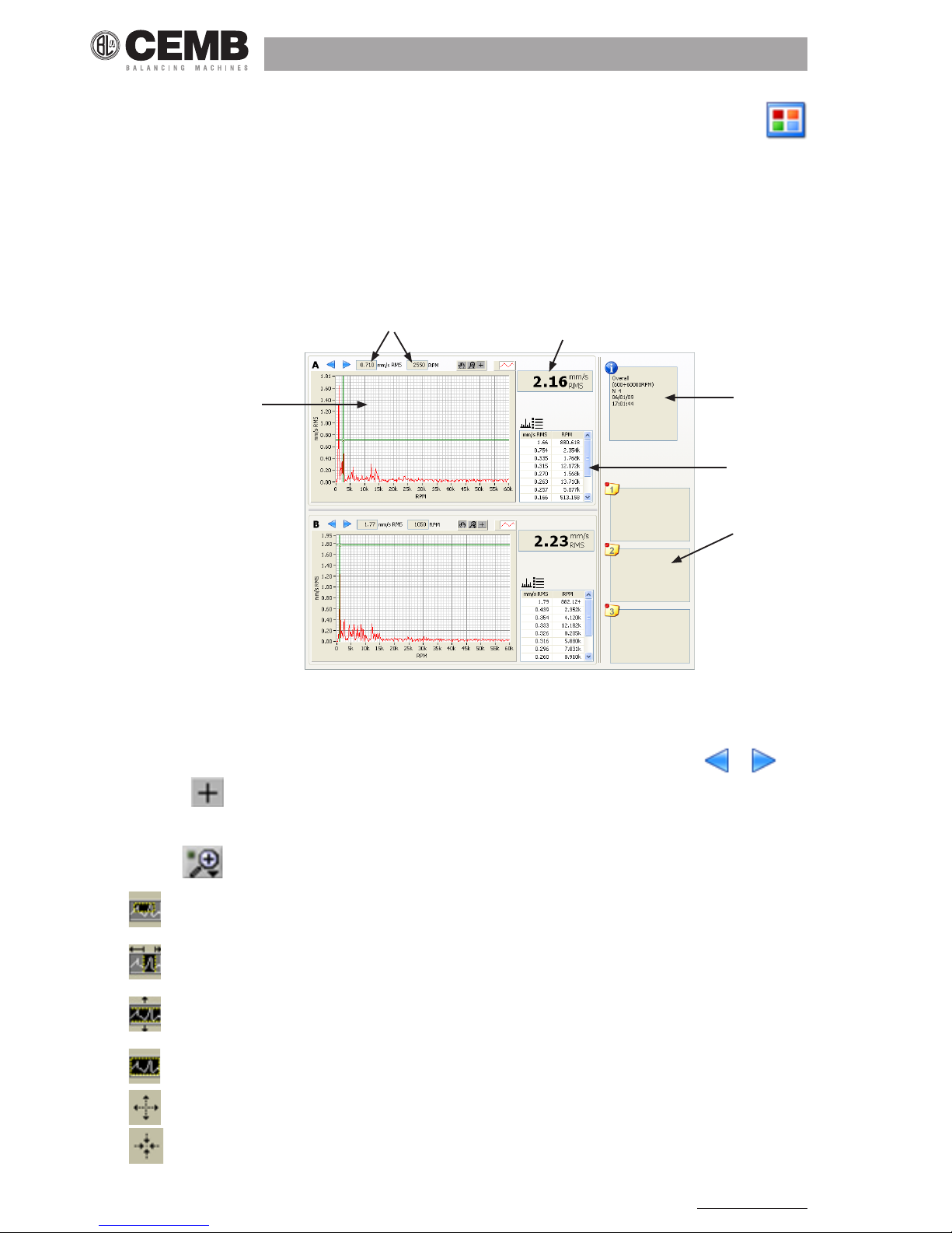
52
N600 - Ver. 2.2 09/2015
10.11 dIsplayInG data present In tHe records
After selecting a le from the records, the contents can be displayed in a clear and detailed manner by pressing the
key.
The various data types will be displayed as follows:
1. spectrum graph (not visible directly on the N100 or N300 instrument)
2. position and value of the cursor
3. overall vibration value
4. list of peak values
5. measurement information and parameters
6. notes associated with the measurements
Overall vibration value measurement:
10.12 specIFIc FunctIons For tHe spectrum GrapHs
• Cursor
The graph has a cursor that can be moved left or right one step at a time by clicking on or pressing
By selecting , it is possible to click on the cursor directly and, by holding down the left mouse key, quickly drag it to
the desired position.
• Zoom
By clicking it is possible to choose from various zoom options:
> (enlarge rectangle) : the rectangle to be enlarged can be selected by clicking on one point and dragging the
cursor
> (zoom x) : the portion of the x axis to be enlarged can be selected by clicking on one point and moving the cursor
horizontally
> (zoom y) : the portion of the y axis to be enlarged can be selected by clicking on one point and moving the
cursor vertically
> (autoscale) : by clicking on the graph the extremes of the axes will automatically be set to the most suitable
values, based on that displayed
> (zoom in) : clicking in one point enlarges the zone around it
> (zoom out) : clicking in one point displays a larger area around it.
2
3
5
4
6
1

Vibration equipment division
53
N600 - Ver. 2.2 09/2015
1
2
3
4
5
• Moving the graph in the window
After having selected , it is possible to click on one point of the graph and, without releasing the mouse button,
move the whole graph within the window. In practice this changes the minimum and maximum extremes of both axes,
without altering the scale. By dragging the cursor out of the window, the graph returns to the position it was in previously.
the minimum and maximum values oF the axes can be modiFied individually by simply clicking on them and entering a
new value using the keyboard.
10.13 syncHronous VIbratIon Value measurement (only For n100 and n300 Instruments)
1. amplitude of the synchronous vibration value
2. phase of the synchronous vibration value
3. frequency of the synchronous vibration value
4. measurement information and parameters
5. notes associated with the measurements
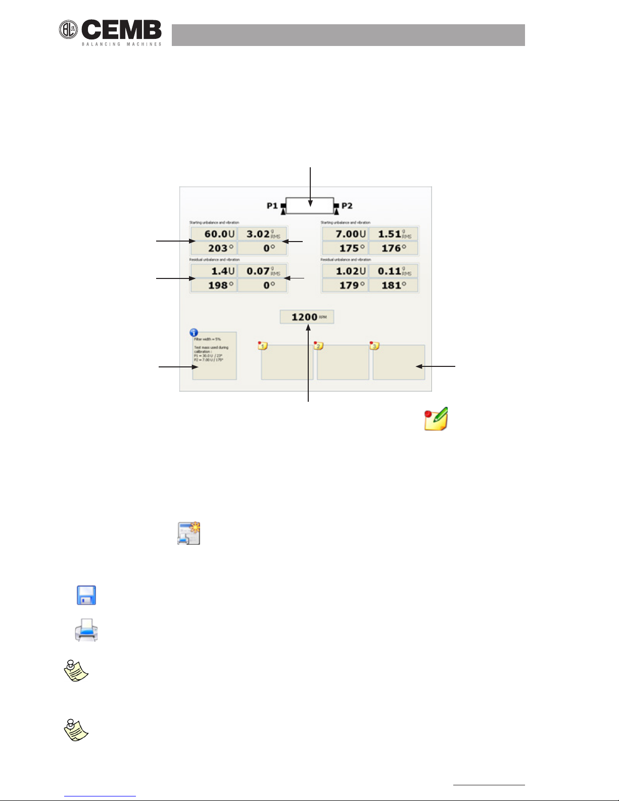
54
N600 - Ver. 2.2 09/2015
1
2
4
7
3
5
8
6
10.14 balancInG data (only For n300 and n600 Instruments)
1. type of balancing (on one or two planes)
2. value (in generic U units) and phase of the initial imbalance
3. value and phase of the initial vibration
4. value (in generic U units) and phase of the nal imbalance (that is to say after balancing)
5. value and phase of the nal vibration (that is to say after balancing)
6. velocity of the rotating part
7. balancing information and parameters
8. notes associated with balancing
The notes associated with each measurement can be entered or edited at any time by pressing
.
This is a valid help in the post-data analysis stage: the user can add comments or notes related to the values or type of
measurement, but also regarding the acquisition conditions. Reminders for future work can be added, or other important
notes. For example, in the case of balancing it is recommended to specify what physical units (mg, g, kg, g
•
mm, g• cm, g•
m…) the generic U units correspond to.
10.15 GeneratIon and prIntInG oF certIFIcates (reports)
CEMB N-Pro software can be used to create and print customised certicates of vibration analysis and balancing results
with extreme ease. Press the key, then select a model (template) for the certicate to be generated. The model is a
simple HTML le that the same user can create and customise to suit his own needs using any HTML editor. The CEMB N-
Pro program generates the report automatically replacing some preset codes in the template with the corresponding values
of the measurement displayed. The result is then displayed in a window and the following functions are enabled:
• : to save the report just generated, specifying the name and position
• : to print the report displayed, selecting a printer from those installed on the PC.
iF a virtual pdF printer is installed on the pc (e.g. pdFcreator, …), select that to obtain a copy oF the certiFicate
in pdF Format instead oF a hard copy. it can then be named and saved on the hard disk in the desired location, so
that it can be Filed or even sent by e-mail. a hard copy can be obtained at a later date iF required by printing oFF a
copy oF the pdF document.
to assist users, the cemb n-pro program includes some example templates that can be used as a base to create
customised reports. these models are located in the sub-Folder named report templates in the n-pro directory in
which the program is installed.

Vibration equipment division
55
N600 - Ver. 2.2 09/2015
————————————————————————————————————————————————————
warnInG!
IF you wIsH to customIse one oF tHe templates present In tHe report templates Folder,
It Is best to saVe tHe edIted model wItH anotHer name or In a dIFFerent Folder. tHIs Is because subsequent n-pro soFtware
updates wIll oVerwrIte tHe templates dIstrIbuted by cemb wItH tHe proGram.
————————————————————————————————————————————————————
the list oF codes that can be used in the templates and their meanings, and some suggestions For the creation oF
customised certiFicates, are given in appendix e.
10.16 GeneratInG and prIntInG multIple measurement certIFIcates (multI-report)
This function allows to group in a single document a series of measurements taken at subsequent times, even for different
points of different machines. The certicate can be fully customised thanks to the extension of the template concept. Prede-
ned codes for multi-reports are composed of two parts:
• the code related to the information to be replaced (identical to a single measurement report)
• the sequential number of the measurement to which the code refers
The steps for generating a multi-report are very simple:
1. use ‘CTRL + click’ or ‘SHIFT + click’ to select measurements from the data records to be included in the multi-report,
which must be contained in a single folder
2. press the button
3. select the desired template
th e des cri pt ion , l ist a nd me an ing oF co de s t hat ca n be us ed in mu lti-re port te mpl ates ar e sho wn in
ap pend ix e.

56
N600 - Ver. 2.2 09/2015
Appendix A
specIFIcatIons
Instrument
• Dimensions: ca. 225 x 200 x 50 mm
• Weight: 1.4 kg
Operating range
• Temperature: -10°C to +50°C
• Air humidity: 0 to 95% without condensation
Power supply
• 6 Ah rechargeable lithium battery
• Charging time: less than 5 hours (with battery fully discharged)
• Power supply/battery charger for 100-240V, 50/60 Hz (24V, 1.5 A)
• Battery life: more than 8 hours with normal instrument use
Display
• 7” TFT colour LCD, LED backlit
• A/D converter: 24-bit resolution
Keypad
• 28 keys, including 6 function keys
Inputs
• 2 independent and simultaneous measuring channels (accelerometer, velocimeter, non-contact, any dynamic signal of
max. 5V-PP)
• 1 photocell channel (speed and angular reference)
• 2 USB ports for data exchange
Connectable sensors
• Accelerometer
• Velocimeter
• Proximity sensor
• Generic with max. 5V-PP signal
• Photocell 30 - 250,000 RPM
Bluetooth portable printer (optional)
• Dimensions: 146 x 88 x 65 mm
• Weight: 0.360 kg (without paper roll)
• Printing on normal or adhesive paper
• Paper width: 57.5 mm ± 1 mm
Functions
• Total vibration measurement (acceleration, speed, displacement)
• Vibration phase measurement
• Vibration analysis in frequency domain
• Total vibration monitoring in relation to time or speed (Bode diagram)
• Balancing of rotors in operating condition (1 or 2 planes)
• Waveform
Measurement mode
• Effective value (RMS)
• Peak value (Pk)
• Peak-to-peak value (PP)

Vibration equipment division
57
N600 - Ver. 2.2 09/2015
Units of measure
• Acceleration: [g]
• Speed: [mm/s] or [mils]
• Displacement: [µm] or [mils]
• Frequency: [Hz] or [RPM]
Vibrometer function
• Total vibration measurement
• Maximum frequency settable (100; 500; 1000 Hz; 2.5; 5; 10 KHz)
• Basic vibration value and phase measurement 1x
• Rotor speed measurement
FFT function (frequency analysis)
• FFT analysis (manual/trigger)
• Maximum frequency settable (100; 500; 1000 Hz; 2.5; 5; 10 KHz)
• Resolution (100; 200; 400; 800; 1600; 3200 lines)
• Number of means: 1 to 16
• List of main peaks
Monitor function - Data Logger
• Recording and indication of the trend of the total vibration value over time
• Storage and display of the trend of the vibration phase as the rotation speed changes
Balancing function
• Number of correction planes: 1 to 2
• Graphic measurement stability indicator
• Step-by-step guided balancing procedure with the possibility of interim editing and modications
• Vectorial unbalance split
• Correction by adding or removing material
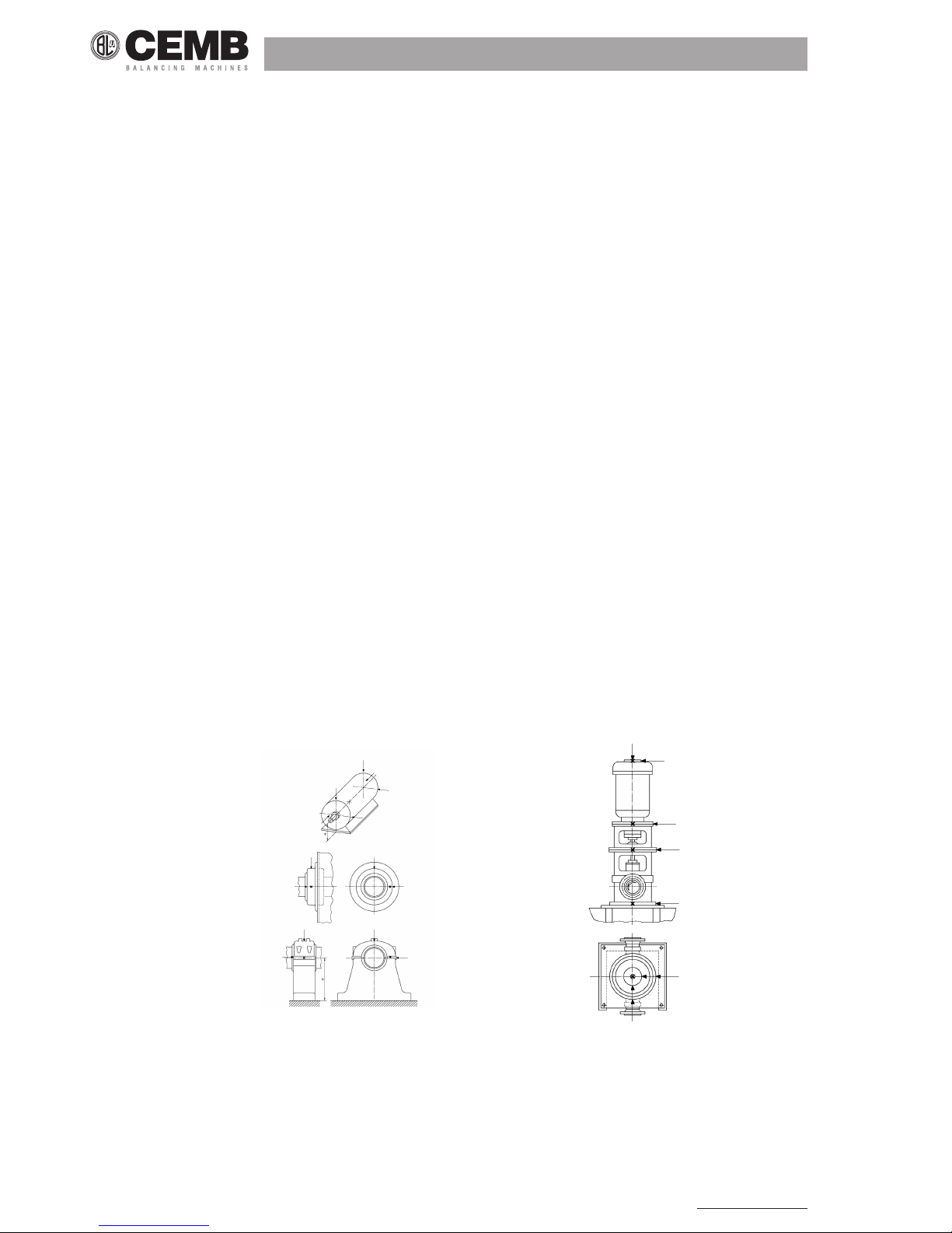
58
N600 - Ver. 2.2 09/2015
Appendix B
eValuatIon crIterIa
UNI ISO 10816-3 Mechanical vibration - Evaluation of machine vibration by measurements on non-rotating parts - Part 3:
Industrial machines with nominal power above 15 kW and nominal speeds between 120 r/min and 15 000 r/min when measured in situ.
IntroductIon
ISO 10816-1 constitutes the basic document that describes the general requirements for evaluation of vibration in different
types of machinery when the vibration measurements are made on non-rotating parts. It provides specic guidance to assess the severity of the vibration measured on bearings, bearing supports or industrial machine casings when the measurements are made in situ.
measurement poInts
Normally, the measurements should be made on the visible parts of the machine which are usually accessible. Due care
should be taken so that the measurements are reasonably representative of vibration of the bearing seat and do not lead to
any local resonance or amplication. The vibration measurement positions and directions must be such as to offer adequate
sensitivity to the dynamic forces of the machine. Generally, this requires two orthogonal radial measurement positions on
each bearing cap or support as illustrated in Figures 1 and 2.
The sensors can be arranged in any angular position on the bearing housings or supports. For horizontally mounted machines, it is generally preferable to arrange the sensors in vertical and horizontal position. For inclined or vertically mounted
machines, the position that gives the maximum vibration reading, normally in the direction of the exible shaft, must be one
of those used. In some cases, measurement in axial direction is also advisable.
On a bearing cap or support, only one sensor can be used instead of the more usual pair of orthogonal sensors if it is known
that this sensor provides sufcient information on the machine vibration amplitude. However, precautions must be taken
when evaluating vibration using only one sensor at the level of a measurement plane, as you risk it not being oriented to
provide a reasonable approximation of the maximum value on this plane.
Figure 1 Measurement points Figure 2 Measurement points for
vertical machine units
classIFIcatIon accordInG to macHIne type, nomInal power or sHaFt HeIGHt
Signicant differences in design, type of bearings and type of support structures require a division into different machine
groups (as regards the shaft height, see ISO 496). The machines in the 4 groups below may have a horizontal, vertical or

Vibration equipment division
59
N600 - Ver. 2.2 09/2015
inclined shaft and may be mounted on rigid or exible supports.
Group 1: Large machines with nominal power above 300 kW or electrical machines with shaft heights ≥ 315 mm.
These machines normally have sleeve bearings. The range of operating or nominal speeds is relatively broad
with ranges from 120 r/min to 15 000 r/min.
Group 2: Medium-sized machines with nominal power above 15 kW up to and including 300 kW or electrical machines
with shaft heights from 160 mm up to ≥ 315 mm.
These machines normally have rolling bearings and an operating speed above 600 rpm.
Group 3: Pumps with n rotors and separate motor (mixed or axial ow centrifugal pumps) with nominal power above
15 kW. The machines in this group may have sleeve or rolling bearings.
Group 4: Pumps with n rotors and incorporated motor (mixed or axial ow centrifugal pumps) with nominal power abo-
ve 15 kW. The machines in this group normally have sleeve or rolling bearings.
classIFIcatIon accordInG to support FlexIbIlIty
The exibility of the support unit in the specied directions is classied considering two possibilities:
• rigid supports
• exible supports
These support conditions are determined by the ratio between the exibility of the machine and that of its foundation. If the
natural lowest frequency of the combined machine-support system in the measuring direction is greater by at least 25% than
the main excitation frequency (in most cases, this is the rotation frequency) in this direction, the support system may be
considered rigid. All other support systems may be considered exible.
Typical examples: large and medium-sized electrical motors, mainly with low speeds, have rigid supports, while turbo generators and compressors with power above 10 MW and vertical machine units normally have exible supports.
In certain cases, a support may be rigid in one direction and exible in the other. For example, the natural lowest frequency
in vertical direction may be well above the main excitation frequency, while the natural frequency in horizontal direction may
be considerably lower. Such a system would be rigid on the vertical but exible on the horizontal plane. In these cases, the
vibration should be evaluated according to the classication of the support that corresponds to the measuring direction.
If the machine-support system class cannot easily be determined from drawings or calculated, it can be determined with
tests.
eValuatIon zones
The following evaluation zones are dened to allow qualitative vibration evaluation of a given machine and to provide guidelines for any action to be taken.
Zone A: the vibration of newly commissioned machines normally falls within this zone
Zone B: machines with vibration within this zone are normally considered acceptable for unrestricted long-term operation.
Zone C: machines with vibration within this zone are normally considered unsatisfactory for long-term continuous opera-
tion. Generally, the machine may be operated for a limited period in this condition until a suitable opportunity
arises for remedial action.
Zone D: vibration values within this zone are normally considered to be of sufcient severity to cause damage to the
machine.
The numerical values specied are not intended to serve as the only basis for acceptance specications, but should be
agreed upon between the machine manufacturer and the customer. Nevertheless, the vibration limits for the zone boundaries provide guidelines for ensuring that gross deciencies or unrealistic requirements are avoided. In certain cases, particular construction solutions may be adopted for a given machine, which would require adopting different values (greater
or smaller) for the zone limits. In these cases, the machine manufacturer generally needs to explain the reasons and, in
particular, conrm that the machine would not be damaged by operation at higher vibration values.

60
N600 - Ver. 2.2 09/2015
eValuatIon zone lImIts
Table A.1
Classication of the vibration severity zones for Group 1 machines: Large machines with nominal power above 300 kW but
not greater than 50 MW or electrical machines with shaft heights ≥ 315 mm
Support class Zone limit Effective displacement, µm Effective speed (mm/s)
Rigid
A/B 29 2,3
B/C 57 4,5
C/D 90 7,1
Flexible
A/B 45 3,5
B/C 90 7,1
C/D 140 11,0
Table A.2
Classication of the vibration severity zones for Group 2 machines: Medium-sized machines with nominal power above 15
kW up to and including 300 kW or electrical machines with shaft heights from 160 mm up to ≤ 315 mm
Support class Zone limit Effective displacement, µm Effective speed (mm/s)
Rigid
A/B 22 1,4
B/C 45 2,8
C/D 71 4,5
Flexible
A/B 37 2,3
B/C 71 4,5
C/D 113 7,1
Table A.3
Classication of the vibration severity zones for Group 3 machines: Pumps with n rotors and separate motor (mixed or axial
ow centrifugal pumps) with nominal power above 15 kW
Support class Zone limit Effective displacement, µm Effective speed (mm/s)
Rigid
A/B 18 2,3
B/C 36 4,5
C/D 56 7,1
Flexible
A/B 28 3,5
B/C 56 7,1
C/D 90 11,0
Table A.4
Classication of the vibration severity zones for Group 4 machines: Pumps with n rotors and incorporated motor (mixed or
axial ow centrifugal pumps) with nominal power above 15 kW
Support class Zone limit Effective displacement, µm Effective speed (mm/s)

Vibration equipment division
61
N600 - Ver. 2.2 09/2015
Rigid
A/B 11 1,4
B/C 22 2,8
C/D 36 4,5
Flexible
A/B 18 2,3
B/C 36 4,5
C/D 56 7,1

62
N600 - Ver. 2.2 09/2015
Appendix C
a rapId GuIde to InterpretInG a spectrum
typIcal cases oF macHIne VIbratIons
1. preliminary rapid guide
Measured values during control
f = vibration frequency [cycles/min] or [Hz]
s = shift amplitude [μm]
v = vibration speed [mm/s]
a = vibration acceleration [g]
n = piece rotation speed [rpm]
Frequency data Causes Notes
1) f = n Unbalances in rotating
bodies
Intensity proportional to unbalance, mainly in the radial
direction, increases with speed
Rotor inection Axial vibrations sometimes sensitive
Resonance in rotating bodies Critical speed near n with very high intensity
Roller bearings mounted with
eccentricity
Recommend balancing the rotor on its own bearings
Misalignments Considerable axial vibration also present, greater than
50% of the transverse vibration; also frequent cases of
f = 2n, 3n
Eccentricity in pulleys, gears,
etc.
When the rotation axis does not coincide with the
geometric axis
Irregular magnetic eld in
electrical machines
Vibration disappears when power is cut off
Belt length an exact multiple
of the pulley circumference
Stroboscope can be used to block belts and pulleys at
the same time
Gear with defective tooth An unbalance vibration often also intervenes
Alternating forces Second and third harmonic present
2) f ≅ n with knocking Mechanical unbalance defect
superimposed on irregular
magnetic eld
In asynchronous motors, the knocking is due to
running

Vibration equipment division
63
N600 - Ver. 2.2 09/2015
3) f ≅ (0,40 ÷ 0,45) n Defective lubrication in
sleeve bearings
Faulty roller bearing cage
For high n, above the 1° critical level
Check with stroboscope
Precision journal movement (oil whirl)
Check for harmonics
4) f = ½ n Mechanical weakness in
rotor
Sleeve bearing shells loose
Mechanical yield
This is a sub-harmonic, often present but hardly ever
important.
f = 2n, 3n, 4n and semi-harmonics also often present
5) f = 2n Misalignment
Mechanical looseness
There is strong axial vibration
Loose bolts, excessive play in the mobile parts and
bearings, cracks and breaks in the structure: there are
upper grade sub-harmonics
6) f is an exact multiple
of n
Roller bearings misaligned or
forced in their housings
Defective gears
Misalignments with excessive
axial play
Rotors with blades (pumps,
fans
Frequency = n x number of spheres or rollers
Check with stroboscope
f = z n (z = number of defective teeth)
Because of general wear, teeth badly made if z = total
number of teeth
Often caused by mechanical looseness
f = n x number of blades (or channels)
7) f is much greater
than n, not an
exact multiple
Damaged roller bearings
Excessive wear on sleeve
bearings
Belts too tight
Multiple belts not
homogeneous
Low load gears
Rotors with blades for uid
management (cavitation,
reux, etc.)
Unstable frequency, intensity and phase.
Axial vibration
Completely or locally defective lubrication
Audible screech
Characteristic audible screech
Run between the belts
Teeth knock together because of insufcient load;
unstable vibration
Unstable frequency and intensity
f = n x number of blades x number of channels
Frequent axial vibration.
8) f = natural frequency
of other parts
Excessive play on sleeve
bearings
Belts disturbed by vibrations
from other parts
Oil whip caused by vibrations in other parts
Check with stroboscope
Examples: eccentric or unbalanced pulleys,
misalignments, rotor unbalances
9) f unstable with
knocking
Multiple belts not
homogeneous
Belts with multiple joints
Unstable intensity
10) f = n
c
n ≠ n
c
( nc = critical speed of shaft)
Roller bearings.
For rotors above the 1st critical speed
(nr = mains frequency)
Electric motors, generators
Harmonics also present
12) f = fc < n or
f = 2 f
c
Belt with defective elasticity
in one area
fc is the belt frequency
fc = π D n / l (D = pulley diameter; l = belt length)
Considerable axial vibrations, more than 10% of the transverse vibration, may be caused typically by:
• misalignment (more than 40%)
• shaft inection, especially in electrical motors
• defective thrust bearings

64
N600 - Ver. 2.2 09/2015
• elliptic eccentricity in the electric motor rotor
• forces deriving from tubing
• distorted foundations
• wear in stufng box seals, etc.
• rotor side rubbing
• defective radial bearings
• defective coupling
• defective belts.
•
2. typical spectra oF viBrations related to the most common deFects
the spectra are in an indicative graphic Form. the n600 equipment produces a diFFerent Form oF graph.
The following are the spectra of typical vibrations, caused by the most common defects found in practical experience.
CPM = shaft rotation speed in rpm
UNBALANCE
MISALIGNMENT
MECHANICAL LOOSENESS/PLAY

Vibration equipment division
65
N600 - Ver. 2.2 09/2015
BELT
GEARS
SLEEVE BEARINGS
ROLLER BEARINGS

66
N600 - Ver. 2.2 09/2015
Θ⋅
−⋅ cos
PD
BDS
=FTF 1
2
Θ⋅
−⋅⋅ cos
PD
BD
N
S
=BPFO 1
2
Θ⋅
⋅⋅ cos
PD
BD
+N
S
=BPFI 1
2
Θ⋅
−⋅
⋅
2
1
2
cos
PD
BD
BD
PDS
=BSP
Θ⋅
+⋅ cos
PD
BDS
=FTF 1
2
Θ⋅
−⋅⋅ cos
PD
BD
N
S
=BPFO 1
2
ELECTRIC MOTORS
3. Formulae For calculating typical Bearing deFect Frequencies
SYMBOLS:
FTF = housing frequency
BPFO = defect on outer track
BPFI = defect on inner track
BSP = defect on roller/ball
The frequencies of bearings can be calculated if we know:
S = number of shaft rpm
PD = primitive diameter
BD = ball/roller diameter
N = number of balls/rollers
Θ = angle of contact
The most common case:
a - xed external ring (rotating internal ring)
b - rotating external ring (xed internal ring)

Vibration equipment division
67
N600 - Ver. 2.2 09/2015
Θ⋅
⋅⋅ cos
PD
BD
+N
S
=BPFI 1
2
Θ⋅
−⋅
⋅
2
1
2
cos
PD
BD
BD
PDS
=BSP
Approximate calculation formulae (± 20%)
FTF = 0.4 x S (a) or 0.6 x S (b)
BPFO = 0.4 x N x S (a) or (b)
BPFI = 0.6 x N x S (a) or (b)
BSP = 0.23 x N x S (N < 10) (a) or (b)
= 0.18 x N x S (N ≥ 10) (a) or (b)

68
N600 - Ver. 2.2 09/2015
Appendix D
laser sensor For cemb n Instruments
Specications
CEMB complete code: 9206812659
Distance from target: 100 - 2000 mm nominal
Current: 30mA nominal
Spare parts
CEMB sensor only, code: 800625541
CEMB cable only, code: 962600025
Connections
Pin 1 Brown Positive power
Pin 3 White Earth
Pin 4 Green Output signal
Instructions for use
Reector position on rotor or shaft.
1. Stick a piece of reective tape on the rotor.
2. It must be at least twice the size of the laser spot.
3. The laser beam should hit the centre of the reector.
4. With the laser connected to the instrument, the LED will come on when the beam passes over the reector and then turn
off. During rotation, the LED will appear to be always on.
Use without reector
In particular conditions, it might not be necessary to use the reector. If there is a difference in reection between one part
of the rotor and the remaining part, use of the reector is not necessary.
If there is more than one target per revolution, the speed measured will not be the correct one.
If you have highly reecting surfaces, position the laser at 90° from the measurement point and colour part of it with a felt-tip
pen.
————————————————————————————————————————————————————
warnInG!
tHe laser measures tHe contrast In reFlectIon and not tHe dIFFerence between colours.
S
ystem response may Vary based on tHe type oF applIcatIon.
I
t Is adVIsable to do a Few tests In order to FInd tHe best solutIon.
————————————————————————————————————————————————————

Vibration equipment division
69
N600 - Ver. 2.2 09/2015
Appendix E
InFormatIon related to tHe creatIon oF customIsed templates (mo
-
dels) For certIFIcates Generated by cemb n-pro soFtware
numerIc codes
When the certicate is created, the CEMB N-Pro software automatically replaces some of the default codes in the template
(#x# format) with corresponding information related to the measurements displayed at the time.
To ensure they are replaced correctly, only the following codes should be used:
#1# Current date
#2# Current time
#3# Note number 1 added to the measurement
#4# Image of the spectrum graph for channel A
#5# Image of the spectrum graph for channel B
#6# Name of the measurement
#7# Path of the le containing the measurement
#8# Serial number of the N100 or N300 instrument
#11# Type of measurement (Pk, PP, RMS)
#12# Type of sensor connected to channel A
#13# Type of sensor connected to channel B
#14# Measurement (overall, 1xRPM, 2xRPM, …)
#15# Number of averages (only for overall measurement)
#16# Synchronous lter width, expressed as a % (only for synchronous measurements
or balancing)
#17# Maximum frequency measured (only for overall measurement)
#18# Number of lines in the spectrum
#19# Note number 2 added to the measurement
#20# Note number 3 added to the measurement
#48# Model of apparatus used to take the measurement (N100, N300)
#49# N100 or N300 apparatus rmware version

70
N600 - Ver. 2.2 09/2015
#50# Frequency and velocity units of measurement
#51# Date on which the measurement was taken
#61# Time at which the measurement was taken
#301# Total vibration value (overall) - channel A
#302# Total vibration value (overall) - channel B
#311# Synchronous vibration value - channel A
#312# Synchronous vibration value - channel B
#321# Synchronous vibration phase - channel A
#322# Synchronous vibration phase - channel B
#331# Synchronous vibration frequency - channel A
#332# Synchronous vibration frequency - channel B
#351# Units of measurement for vibration (g, mm/s, µm, …)
#401# Vibration peak 1 frequency – channel A
#402# Vibration peak 2 frequency – channel A
#...# Vibration peak … frequency – channel A
#405# Vibration peak 5 frequency – channel A
#426# Vibration peak 1 value – channel A
#427# Vibration peak 2 value – channel A
#...# Vibration peak … value – channel A
#430# Vibration peak 5 value – channel A

Vibration equipment division
71
N600 - Ver. 2.2 09/2015
#451# Vibration peak 1 frequency – channel B
#452# Vibration peak 2 frequency – channel B
#...# Vibration peak … frequency – channel B
#455# Vibration peak 5 frequency – channel B
#476# Vibration peak 1 value – channel B
#477# Vibration peak 2 value – channel B
#...# Vibration peak … value – channel B
#480# Vibration peak 5 value – channel B
#601# Initial unbalance value on plane P1 (in U units)
#602# Initial unbalance phase on plane P1 (in degrees °)
#603# Initial vibration value on plane P1
#604# Initial vibration phase on plane P1 (in degrees °)
#605# Current (nal) unbalance value on plane P1 (in U units)
#606# Current (nal) unbalance phase on plane P1 (in degrees °)
#607# Initial unbalance value on plane P2 (in U units)
#608# Initial unbalance phase on plane P2 (in degrees °)
#609# Initial vibration value on plane P2
#610# Initial vibration phase on plane P2 (in degrees °)
#611# Current (nal) unbalance value on plane P2 (in U units)
#612# Current (nal) unbalance phase on plane P2 (in degrees °)
#613# Balancing speed
In the case of multi-reports (certicates produced by grouping together data from N different measurements) #x-y# format
codes must be used, where:
• x: numeric code listed in the previous table
• y: sequential number of the measurement of which the multi-report is composed (1, 2, … N)
For example:
> #6-1# : name of measurement No. 1 of the multi-report
> #11-2# : type of measurement No. 2 of the multi-report
> …

72
N600 - Ver. 2.2 09/2015
suggestions For customising certiFicates
The HTML model (template) used to create the certicates leaves clients free to customise the certicates distributed by
CEMB together with the program, or to create new ones as desired. Clients with special requirements can insert logos or
images and change the size and colour of the wording themselves.
As these templates are HTML documents they should be created or edited using appropriate programs known as HTML edi-
tors. They are used in a similar manner to normal word processing programs (Microsoft Word, Openofce Writer, etc), with
the exception that documents are generated and saved directly in HTML format; this means that the document’s graphic
appearance remains unaltered when saved. On the contrary, if a word processing program is used and the document is
then saved in HTML format, the alignment, spacing, sizes, etc may be altered after being converted and saved and the nal
HTML model may not turn out exactly as desired. Users of Microsoft Word 2000 or higher will have experienced this situation
frequently.
Various HTML editors are available, including:
• KompoZer: multilingual, it can be downloaded free of charge from the website http://www.kompozer.net/
• W3C Amaya: multilingual, it can be downloaded free of charge from the website http://www.w3.org/Amaya/
• Mozilla Composer: multilingual, part of the Mozilla Seamonkey suite, it can be downloaded free of charge from the
website http://www.seamonkey-project.org/
• Adobe Dreamweaver: multilingual, available at a cost.
To assist users, KompoZer is included in the CD together with the CEMB N-Pro software.
creation oF certiFicates in pdF Format
To generate certicates in PDF format, install a virtual PDF printer on the PC and select it after pressing the key in the
CEMB N-Pro software.
If you do not yet have this type of printer, PDFCreator can be installed, which can be downloaded free of charge from the
website http://sourceforge.net/projects/pdfcreator/
Once installed a new printer named PDFCreator will be displayed in the ‘Printers and fax’ window alongside the real printers
connected to the PC.

BALANCING ACCURACY OF RIGID ROTORS
are different according to whether the rotor may be considered
rigid or flexible, similarly, the balancing accuracy or tolerance
is different in the two cases. Suffice to say that in a flexible
rotor, the effect of unbalance is amplified by the elasticity in
such a way as to generate in the pedestals different forces than
those created by a rigid rotor with the same unbalance. We can
deduce, all other conditions being equal, that the balancing
tolerances of the two cases will be different in the presence of
equal forces or vibrations on the pedestals.
The contents of this pamphlet may be considered to be valid
only for rigid rotors, unless otherwise specified.
UNIT OF MEASUREMENT OF BALANCING
TOLERANCE
Balancing tolerance is given by the product of the maximum
permissible unbalance by its distance from the rotational axis.
If the balancing tolerance is divided by the weight of the rotor,
we obtain the “specific unbalance”. This is also called the
“residual permissible eccentricity” as, in the case of static
unbalance, it expresses the eccentricity of the rotor’s barycentre
from the rotational axis caused by the permissible unbalance.
The purpose of balancing is to improve the distribution of
the mass of a rotor so that it may rotate on its bearings
without creating unbalance centrifugal forces higher than
a predetermined permissible value.
This aim can and must be attained only to a certain degree as,
even after balancing, residual unbalance will inevitably persist.
Just as when machining a piece in a workshop it is never possible
to mach drawing sizes with perfect exactness and it is necessary
to predetermine a “machining tolerance”, which varies in
accordance to the requirements of each single piece, also when
balancing, the precision obtained has to suit the needs of each
single piece, which is achieved by fixing a “maximum
permissible residual unbalance” or “balancing tolerance”.
It is obvious that an insufficiently balanced piece will cause
intolerable vibrations with all consequent malfunctions or
damage. However, it would be clearly useless to balance a rotor
to a degree of quality greater than required for a regular and
normal operation of the machine incorporating that part, by using
a balancing machine to its peak precision. In fact, exaggerating
the quality requirements would only result in a waste of time
and a higher balancing cost, without improving the quality of
the rotor.
When fixing the balancing tolerance, the concept of
“reproducibility” should also be borne in mind, i.e. the minimum
value that can be certainly reproduced on repeated testing. For
example: if with the simple operation of disassembling and
reassembling a piece on the balancing machine or of balancing
it at different times on the machine itself there is a variation in
eccentricity of 5 microns, it is quite useless to balance that piece
with a much greater precision than 5 microns.
It is therefore necessary to calculate and prescribe the
technical and economically most effective levels of balancing
tolerance for each type of rotor.
The drawing should, therefore, always show:
- the value of the maximum permissible residual unbalance
for each of the correction planes, with precision;
- where and how compensating weights should be added; or
where material may be removed without damaging the piece;
- the journals that should support the rotor on the balancing
machine;
- the recommended speed range for balancing;
- all other useful data from case to case, that may help to
enable the user to carry out balancing operations quickly
and safely.
This applies to rigid rotors; for flexible rotors, other
specifications should be applied. Just as balancing operations
23826 MANDELLO DEL LARIO (LC) ITALY
SYMBOLS
p (grams) = maximum permissible unbalance
r (mm) = p ’s distance from the rotational axis
P (kg) = rotor weight
n (rpm)= normal service rotational speed
p·r (gr·mm) = maximum permissible residual unbalance
e =
P
rp ⋅
= residual permissible eccentricity (micrometer)
G (mm/s) = balancing grade (see table)

Grade
G ROTOR TYPE
mm/s
0,4 Gyroscopes
Spindles, discs and armature of precision grinders
Spinning spindles
1,0 Small electrical armatures with high level balancing requirements
Tape-recorder and phonograph (gramophone) drivers, cinema projectors
High precision grinding machine drives
Rotors of turbines and compressor of high-speed jet engines
Rotor of steam turbines with high level balancing requirements
2,5 Rotors of steam and gas turbines, of turbo-generators, of turboblowers and of turbine pumps
Merchant ship main turbines
Superchargers, supercompressor for aircraft
Medium and large electrical armatures with high level balancing requirements
Small electrical armatures with a reasonable level of balancing requirements, for high quality domestic electric appliances,dentist’s
drills, aerosols
Small electrical armatures not included in the conditions specified for Grade 6.3
Machine-tool drives
Fans for air-conditioning in hospitals and concert halls
High speed reduction gears (over 1000 rpm) for marine turbines
Disc and drums of computer memories
6,3 Small mass produced electrical armatures in applications where they are not sensitive to vibrations or with antivibrating mounting
Medium and large electrical armatures (with shaft height at least 80 mm) without any special requirements
Machine tools and components of machine tools and of machines in general
Fast moving weaving and spinni ng looms, plaiting machines, centrifuge drums (creams separators, cleansing plants, washing
machines)
Hydraulic machine rotors
Fly-wheels, fans, centrifugal pumps
Reduction gear for merchant navy marine propulsion turbines
Cylinders and rollers for printing machines
Gas turbine rotors for the aeronautical industry
Separated components of engines under special requirements
16 Drive and cardan shafts with high level balancing requirements
Parts for agricultural, grinding and threshing machines
Motor parts for vehicles, commercial vehicles and locomotives (petrol or diesel drive)
Crankshafts complete with fly-wheels and clutches with 6 or more cylinders with high level balancing requirements
Drums for slow centrifuges
Propellers for light boats (motor boats. hydrofoils)
Wheel-rims for car and motorbikes
Normal drive pulleys
Large cylinders for paperworks
Single-piece tools for wood-working machines.
40 Wheels and wheel-rims for cars
Drive shafts and complete axles for vehicles
Crankshafts complete with fly-wheels and clutches for 4-stroke engines with 6 or more cylinders mounted elastically, with piston
speed greater than 9 m/s
Crankshafts complete with fly-wheels and clutches for car, lorry and locomotive engines
Drive shafts for pulleys
Multi-piece tools wood-working machines
100 Complete crankshafts for diesel motor of six or more cylinders with a piston speed greater than 9 m/s
Complete engines for vehicles and locomotives
Crankshafts for 1, 2 or 3 cylinder engines
250 Complete crankshafts for rigidly-mounted, 4 cylinder diesel engines: with piston speed greater than 9 m/s
630 Complete crankshafts for large rigidly-mounted, 4-stroke engines
Complete crankshafts for elastically mounted marine diesel engines
1600 Complete crankshafts for large rigidly-mounted, 2-stroke engines
4000 Complete crankshafts for rigidly-mounted marine diesel engines, with any number of cylinders, with a piston speed lower than 9 m/s
BALANCE QUALITY GRADES FOR VARIOUS GROUPS OF ROTORS
Note: The rotor classes in italics are not included in the ISO standards, but have been added by the Author.
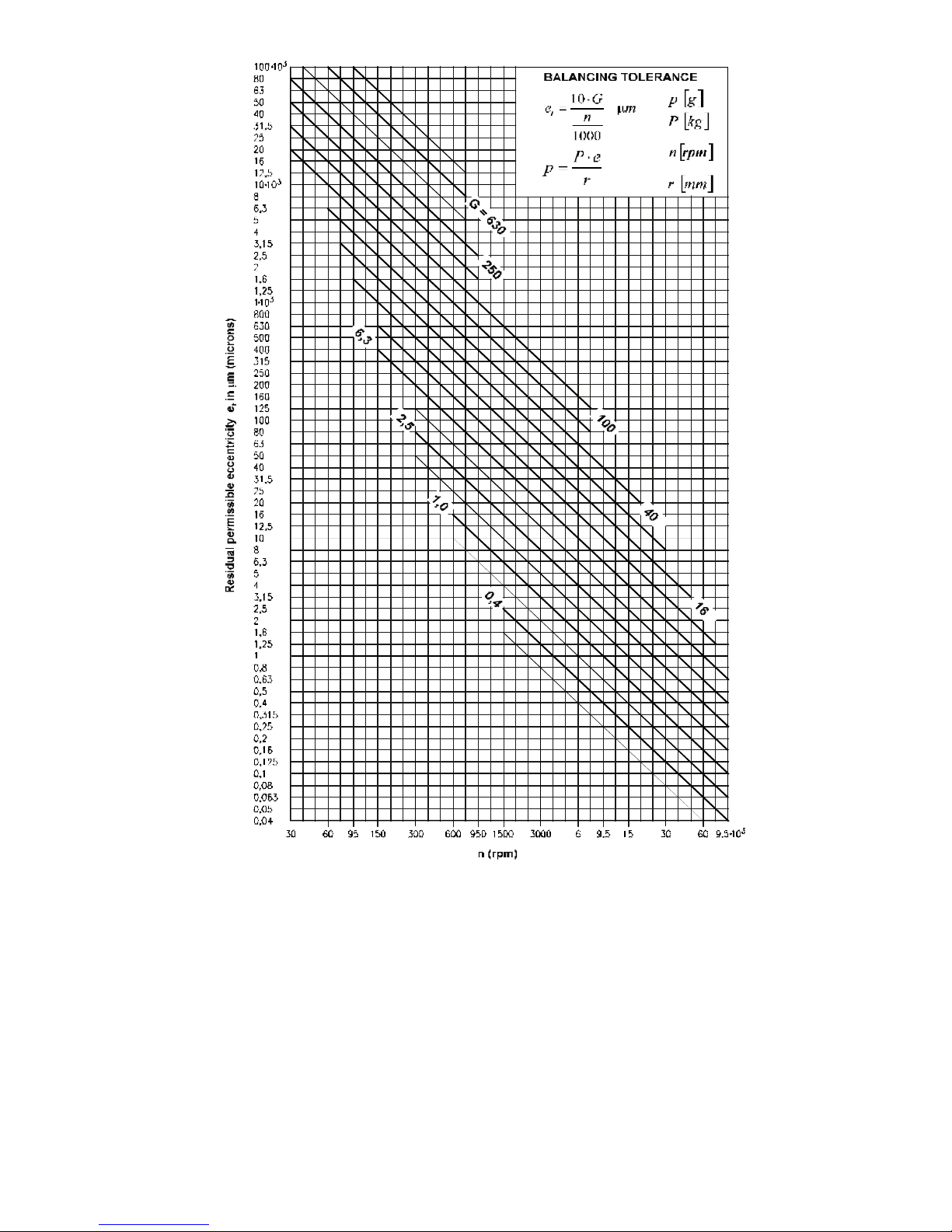
HOW TO USE THE BALANCING TOLERANCE GRAPH
The balancing quality grade G is determined according to the
characteristics of the rotor and the machine on which the rotor
is mounted under normal service conditions (see table).
The residual permissible eccentricity may then be deduced from
the graph, as a function of the rotational speed, in
correspondence with the G grade.
The residual eccentricity is not a fixed value: it may vary for a
given G grade between a minimum and a maximum,
corresponding to the two fine lines above and below the line of
the G grade, according to the rotor type and purpose and to the
construction characteristic of the machine on which the rotor
will be mounted.
The balancing tolerance in gr·mm may be obtained from the
residual eccentricity e (micrometers) multiplied by the rotor
weight P (kg).
The tolerance values obtained are generally a good guide and
sufficient to ensure satisfactory service conditions to a great
extent. Some corrections may, however, be opportune and
sometimes necessary, particularly when the machine has
construction characteristics substantially different from those
of traditional machines of the same category.
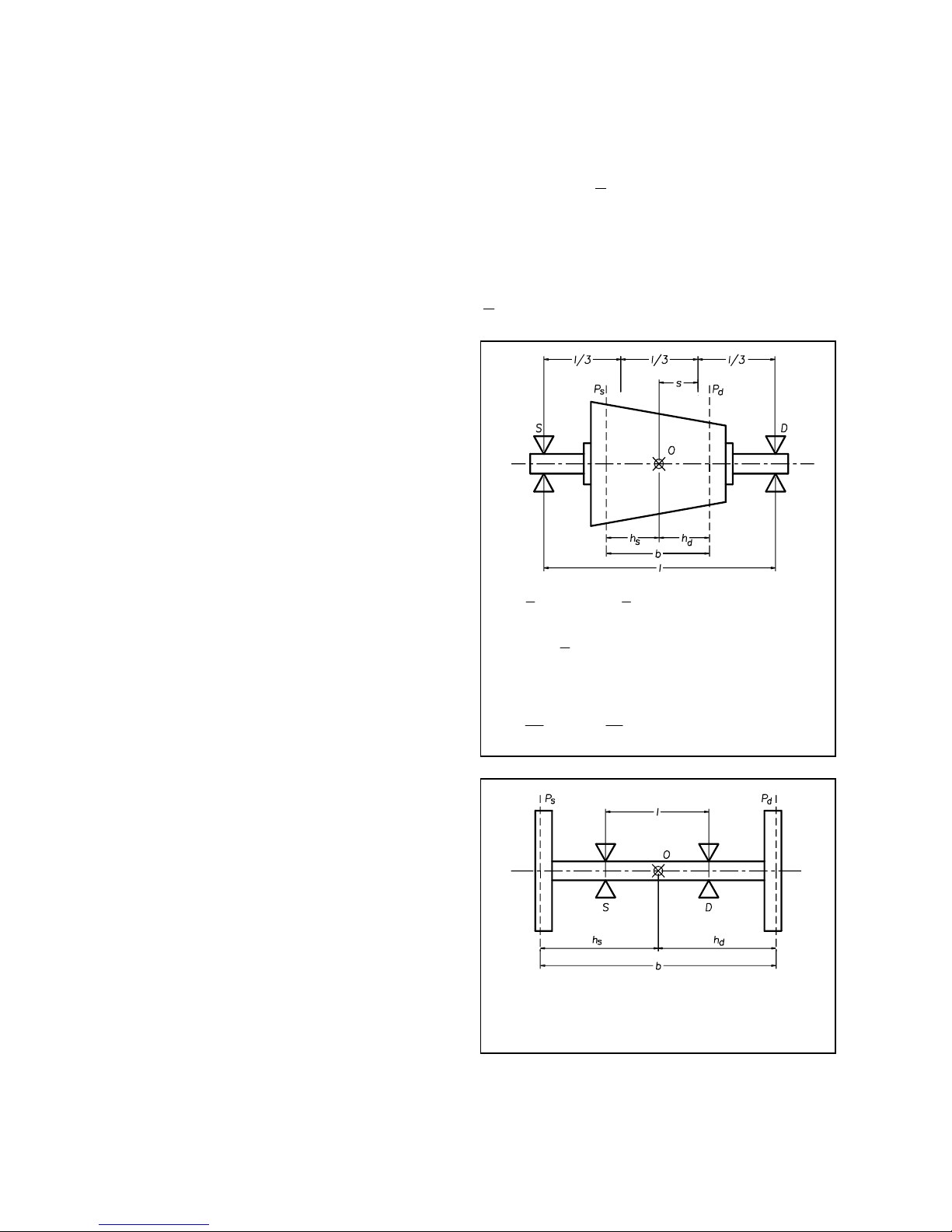
CONDITIONS OF VALIDITY OF THE BALANCING TOLERANCE GRAPH
1. The balancing values refer to the entire rotor; if there are two
planes of correction and if the rotor is approximately symmetrical,
each correction plane should be allotted a tolerance value equal
to half the value found, as long as the correction planes are
symmetrical with respect to the barycentre and the pedestals; in
the case of marked asymmetry in the rotor or in the position of the
correction planes, the residual unbalance must be divided
accordingly between the two planes of correction.
2. The tolerance values arc valid both for static and for couple
unbalance.
3. A rotor should be considered to be rigid over its complete range of
service speeds and in the actual working conditions of the machine
itself (bearings, pedestals, bedplates, foundations, couplings with
other rotors, drive elements, etc.).
NOTE 1 - Balancing grades 0,4 and 1
For class 0,4 and 1 rotors, balancing tolerance must normally be
checked with the direct experimental method.
The influence of the means of rotor drive and of the bearings may be
significant.
NOTE 2 – Use of auxiliary equipment
For rotors that must be mounted on auxiliary shafts or flanges for
balancing, the tolerances shown are only meaningful if, as well as the
unbalance of the auxiliary shaft or flange, the play of the mounting and
the working tolerance of the piece are checked for their concentricity
with the rotational axis, both for the residual unbalances and of the
ultimate shaft. The sum of the residual unbalances and of the plays,
converted into eccentricity values, must, of course, be lower than the
balancing tolerance, as the balancing accuracy obtained would otherwise
be purely illusory.
NOTE 3 - Assembled rotors
For assembled rotors the unbalance of the component parts must be
summed together vectorially, also bearing in mind the unbalance that
derives from the mounting (machining tolerances, clearances, keys,
set screws, etc.).
The unbalance resulting after the assembling should be lower than that
indicated by the graphs for the complete rotor; if it is not, the rotor
should be balanced after assembly, selecting two suitable planes of
correction.
DIVIDING THE PERMISSIBILE RESIDUAL
UNBALANCE BETWEEN TWO CORRECTION
PLANES
In most rotors, a reasonable division of the total permissible
residual unbalance U of the rotor is possible between the two
correction planes using one of the following methods; choose
the method according to the conditions specified.
Us and Ud are used to indicate the respective permissible
residual unbalances for the left and right correction planes (see
figures).
O
indicates the rotor’s barycentre.
1) If
lb
l
<<
3
;
3
l
s <
with
ds
hh ≅ we can consider
UUU
ds
2
1
==
With
ds
hh ≠
but
bhb
s
7,03,0 <<
we can consider
U
b
h
U
d
s
=
;
U
b
h
U
s
d
=
2) If
lb >
it is advisable to consider a greater value of
overall unbalance to be divided as above
DIRECT EXPERIMENTAL METHOD
The most accurate and safest value of the maximum permissible
residual unbalance can only be obtained with direct experiments.
To do this, balance the rotor on a balancing machine as accurately
as possible, then fit it on its ultimate machine in service
conditions. In successive tests, add increasing unbalances, until
the vibrations of the pedestals or of the machine become
significant. Now establish the maximum permissible unbalance
in relation to the value found, e/g. one third.
This testing must be systematic, so as to take all possible cases
of vibration and all possible conditions of the rotor and of the
position of the added unbalances into consideration.
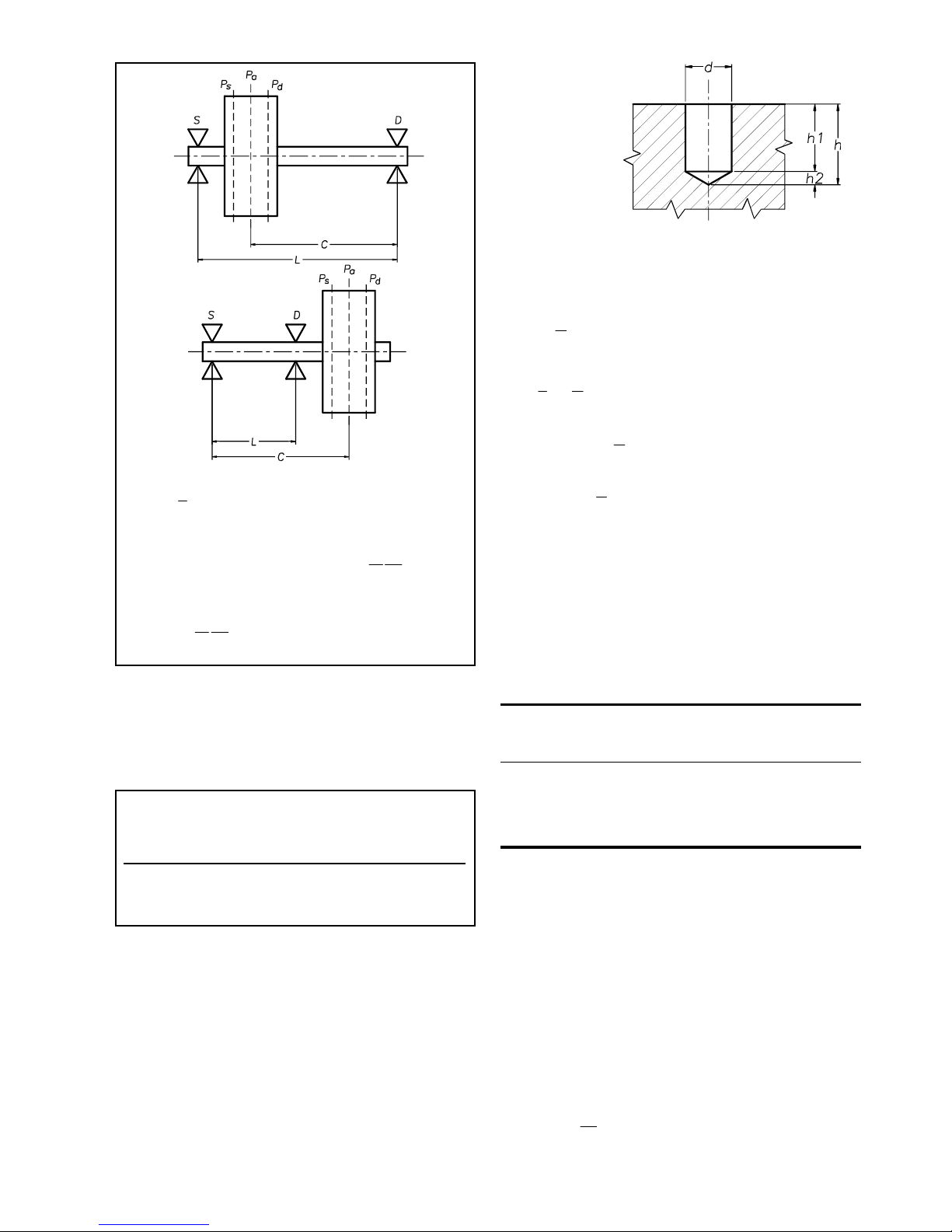
3) If
3
l
b <
it is advisable to use an auxiliary plane P
a
(which may coincide with Ps or Pd) for which the
maximum permissible unbalance is
c
lU
U
a
22
=
furthermore, for planes Ps and P
d
b
lU
UU
ds
432
==
P in grams
d in mm
h1-h2-h in mm
The total weight to
4) The permissibile residual unbalance for one correction
plane is usually given by the product of the overall
permissible residual unbalance of the entire rotor and the
relationship between the distance of the other correction
plane from the rotor’s barycentre and the distance between
the correction planes.
If the rotor does not come under any of the simplified
methods listed, you must follow the general method, which
is valid for any rotor and any position of the correction
planes.
The general method is set out in CEMB Technical Booklet
N° 8 (which can be sent f.o.c. on request), and in International
Standard N° 1940/1 (1986-09-1).
PRACTICAL USE DIAGRAMS FOR
CORRECTING UNBALANCE
DRILLING IN STEEL:
Use diagrams 1 to 5 according to need. Each diagram supplies
the depth of the drill hole (h), as a function of the weight to be
removed (P) and the diameter of the drill bit (d). The curves are
plotted for steel (density 7.85 kg/dm3), taking the conical shape
(120°) of the drill bit into account, using the following criterion:
Unit of measurement:
be removed from a
drill hole is: P = 7.85 10-3 V (where V is the total volume
of the hole) (1) considering that:
21
VVV +=
where
1
2
1
2
h
d
V ⋅
÷
ø
ö
ç
è
æ
⋅π=
(Volume of cylindrical pan) and
2
2
2
23
1hd
V ⋅
÷
ø
ö
ç
è
æ
⋅π=
(Volume of conical part)
21
hhh −=
;
°= 30tan
2
2
d
h
(1) becomes:
÷
ø
ö
ç
è
æ
⋅−
π
⋅=
− 323
1511.0
4
1085.7 dhdP
(2)
DRILLING IN ALUMINIUM, CAST IRON etc.
Once you know the weight that has to be removed, you must
multiply it by a correction coefficient designed to take the
different densities of the materials into account. The resulting
weight is used in diagrams 1 to 5 to determine the correct value
of hole depth (h).
TABLE OF CORRECTION COEFFICIENTS
MAT D Reference Correction coefficient
density (7.85/D)
(Kg/dm3)
ALUMINIUM 2.7 2.91
CAST IRON 7.25 1.09
BRASS 8.5 0.92
COPPER 8.9 0.88
EXAMPLE:
Unbalance to remove P = 10 grams. Drill bit used d = 14 mm.
Rotor material ALUMINIUM. Corrected P value = 10x2.91 =
29.1 Diagram 1 gives us h = 27 mm
CORRECTING BY ADDING WEIGHT TO STEEL:
Use diagram 6. This supplies the weight of a 1 cm long plate, as
a function of the commercial dimensions of thickness (S) and
width (L). Divide the unbalance by the weight obtained from
the diagram to obtain the length (l).
EXAMPLE: Unbalance to add 50 grams
Plate used 50x10 mm.
Diagram 6 gives us a weight of P = 39 grams/cm
therefore
3.1
39
50
==l
cm.


1 - GENERAL DIAGRAM OF WEIGHT REMOVABLE BY DRILLING IN STEEL
(For small weight see diagrams 2 – 3 – 4 – 5)
Cone only
Weight removed in grammes
Hole depth (h) in mm
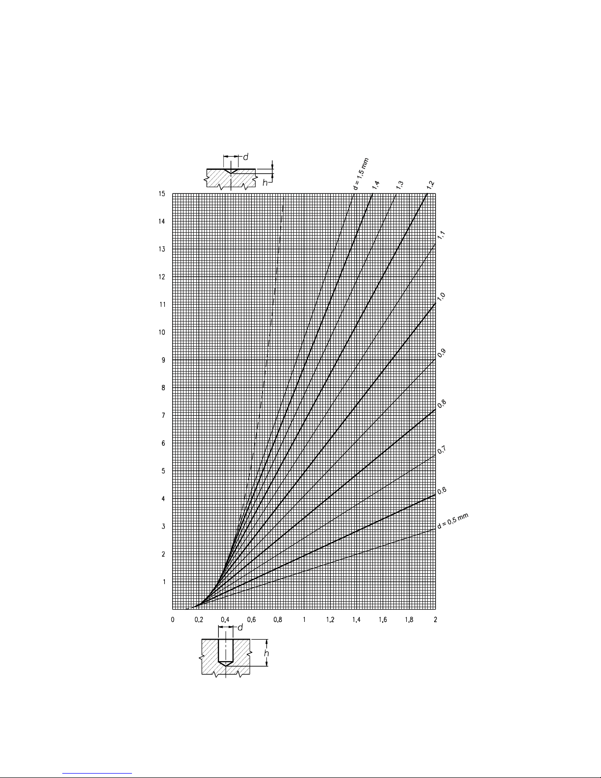
2 - DIAGRAM FOR FINE DRILLING Ø 0,5 – 1,5 mm
Hole depth (h) in mm
Weight of material removed (steel) in milligrammes
Cone only

3 - DIAGRAM FOR FINE DRILLING Ø 1 – 6 mm
Hole depth (h) in mm
Weight of material removed (steel) in grammes
Cone only
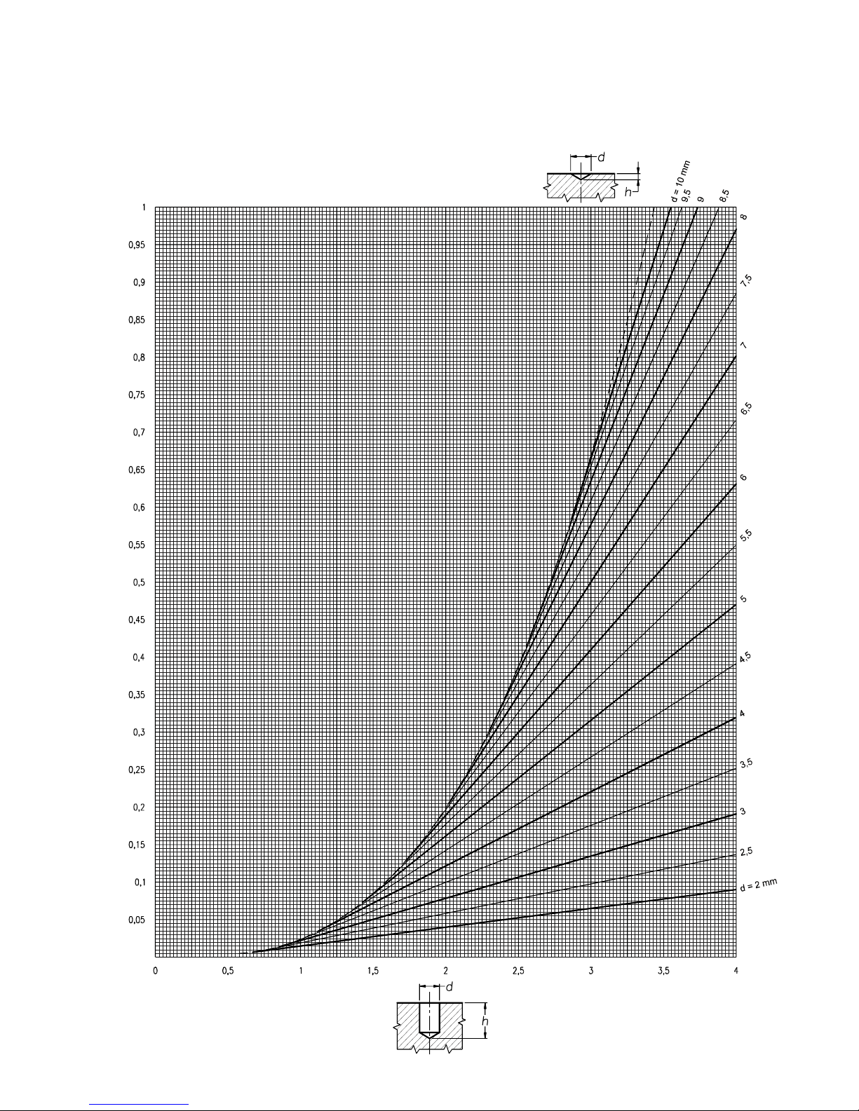
4 - DIAGRAM FOR FINE DRILLING Ø 2 – 10 mm
Hole depth (h) in mm
Weight of material removed (steel) in grammes
Cone only

5 - DIAGRAM FOR FINE DRILLING Ø 5 – 12 mm
Hole depth (h) in mm
Weight of material removed (steel) in grammes
Cone only
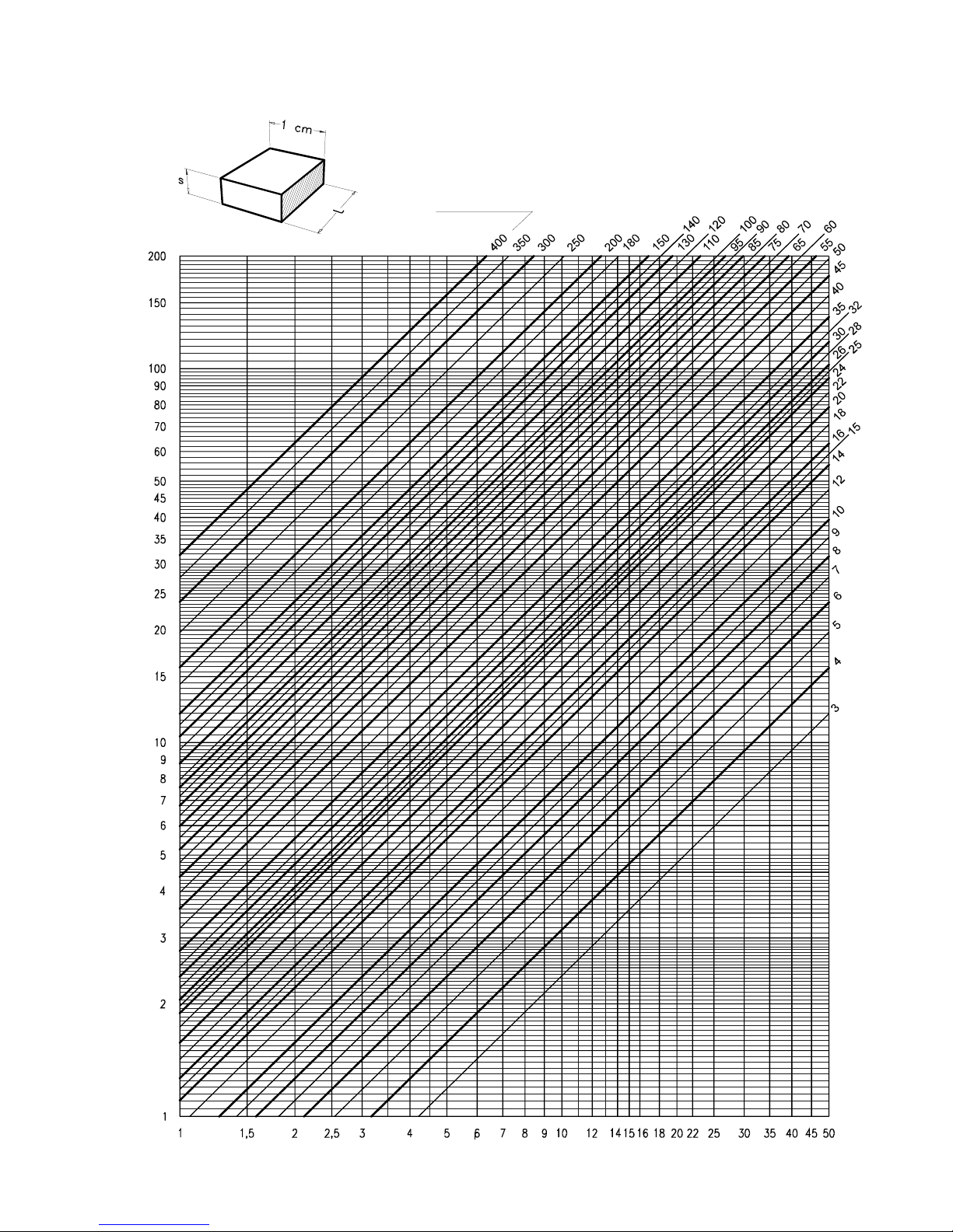
6 - DIAGRAM OF WEIGHT per cm OF A STEEL PLATE AS A FUNCTION OF DIMENSIONS L - s
Thickness of plate (s) in mm
Weight of plate in g/cm
Width of plate (L)
in mm
 Loading...