Campbell Scientific TGA100 User Manual

Download

TGA100 TRACE GAS ANALYZER

USER AND REFERENCE MANUAL

LAST REVISION: 2 August 2004

1 OVERVIEW 12

1.1 System Components 12

1.2 Theory of Operation 13

1.2.1 Optical System 13

1.2.2 Laser Scan Sequence 14

1.2.3 Concentration Calculation 15

1.3 Trace Gas Species Selection 15

1.4 Dual Ramp Mode 15

1.5 User Interface 16

1.6 Micrometeorological Applications 17

1.6.1 Eddy Covariance 17

1.6.2 Flux Gradient 18

1.6.3 Site Means 19

1.6.4 Absolute Concentration / Isotope Ratio Measurements 20

1.7 Specifications 21

1.7.1 Measurement Specifications 21

1.7.2 Physical Specifications 22

2 INSTALLATION 23

2.1 Analyzer Installation 23

2.2 TGA100 PC Installation 24

2.3 Routine Operation 25

2.3.1 Startup Procedure 25

2.3.2 Shutdown Procedure 25

2.3.3 System Checks 26

3 TGA SOFTWARE 27

3.1 General 27

3.2 Startup 27

3.3 Main Menu 27

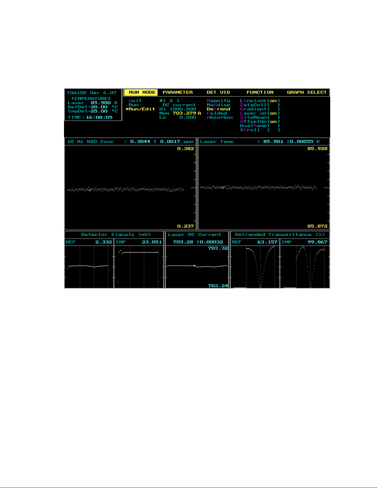
3.4 Real Time Screen 28

3.4.1 Screen Layout 29

3.4.2 Navigating and Editing 30

3.4.3 Run Mode 30

3.4.4 Dynamic Parameters 31

3.4.5 Detector Video 32

3.4.6 Functions 32

3.4.7 Graph Selections 32

3.4.8 Graph Display Limits 33

3.4.9 Quick Keys 33

3.5 Parameter Change Menu 35

3.5.1 Standard Parameter Screens 36

3.5.2 File Output Selection Screen 37

3.5.3 Analog Output Screen 38

3.5.4 Gradient and Site Means Screens 39

3.6 TGA Files 39

3.6.1 Parameter Files 39

3.6.2 10 Hz Concentration Data Files 40

3.6.3 Gradient (Delta Concentration) Files 40

3.6.4 Site Means Files 41

3.6.5 Housekeeping Data File 42

3.6.6 Header Files 43

3.6.7 User Messages 43

4 DETAILED SETUP INSTRUCTIONS 44

4.1 Configuring the System for a Specific Gas Species 44

4.1.1 Laser Selection 44

4.1.2 Reference Gas 44

4.1.3 Detectors 45

4.1.4 Air Gap Purge 46

4.1.5 Polyethylene Sample Cell Liner 46

4.2 Optical Alignment 47

4.2.1 Setting Parameters to Align a New Laser 49

4.2.2 Initial Alignment 49

4.2.3 Horizontal and Vertical Alignment 50

4.2.4 Focus Adjustment 51

4.2.5 Reference Detector Coalignment 51

4.3 Finding the Absorption Line 52

4.4 Laser Mapping 53

4.5 Optimizing Laser Parameters 55

4.5.1 Laser Temperature 55

4.5.2 Zero Current 58

4.5.3 High Current 59

4.5.4 Omitted Data Count 62

4.5.5 Laser Modulation Current 63

4.5.6 Laser Maximum Temperature and Laser Maximum Current 63

4.5.7 Laser Multimode Correction 63

4.6 Optimizing Detector Parameters 64

4.6.1 Detector Gain and Offset 64

4.6.2 Detector Temperature 65

4.6.3 Detector Linearity Coefficients 65

4.7 Calibration 66

5 SAMPLING SYSTEM CONTROL 67

5.1 GRADIENT MEASUREMENTS 67

5.1.1 Gradient Overview 67

5.1.2 Gradient Calculations 68

5.1.3 Real time display 70

5.1.4 Controlling Gradient Valve Assemblies 70

5.1.5 Controlling a Gradient Site Selection Assembly 72

5.1.6 Gradient Mode Parameters 74

5.1.7 Gradient Mode Setup 75

5.2 SITE MEANS MEASUREMENTS 80

5.2.1 Site Means Overview 80

5.2.2 Site Means Calculations 81

5.2.3 Real Time Display 83

5.2.4 Controlling a Site Means Sampling System 83

5.2.5 Site Means Parameters 84

5.3 MASTER/SLAVE OPERATION 85

5.3.1 Master/Slave Setup 85

5.3.2 Master/Slave Operation 86

5.3.3 Shift and Omit Samples 86

6 EDDY COVARIANCE MEASUREMENTS 86

6.1 Overview 86

6.2 Flow Rate and Tubing Size 88

7 AUXILIARY INPUTS AND OUTPUTS 90

7.1 Reading Data from a CSAT3 Sonic Anemometer 90

7.2 Reading Data from a CR9000 90

7.3 Sending Concentration Data to a CR9000 91

7.4 TGA Analog Inputs 91

7.5 PC Analog Inputs 92

7.6 Analog Outputs 92

7.7 Digital Outputs 93

7.8 Excitation Source 93

8 TGA100 OPTIONS 94

8.1 Laser Cooling 94

8.1.1 LN2DEWAR TGA100 LN2 Laser Dewar 94

8.1.2 CRYODEWAR TGA100 Laser Cryocooler System 94

8.2 Lasers 95

8.3 TGAHEAT Temperature Controller 95

9 TGA100 ACCESSORIES 96

9.1 TGA100 Insulated Enclosure Cover 96

9.2 Dewar Evacuation System 96

9.3 Sample Vacuum Pump 96

9.4 Sample Air Dryers 97

9.4.1 General Description 97

9.4.2 Theory of Operation 98

9.4.3 Installation Instructions 98

10 TROUBLESHOOTING 102

10.1 Fiber Optic Diagnostics 102

APPENDIX A. OPTIONS FOR FILE SAVE AND REAL TIME DISPLAY 104

APPENDIX B: DEFAULT PARAMETER FILE 108

1 OVERVIEW

The TGA100 Trace Gas Analyzer measures trace gas concentration in an air sample using tunable diode laser absorption spectroscopy (TDLAS). This technique provides high sensitivity, speed, and selectivity. The TGA100 is a rugged, portable instrument designed for use in the field. It can measure one of a large number of gases by choosing appropriate lasers and detectors. It incorporates several features that make it ideal for measuring fluxes of trace gases using gradient or eddy covariance techniques. A vacuum pump continuously pulls the air sample through the analyzer, which measures the concentration of the trace gas at a 10 Hz rate. The TGA computer provides the user interface; controlling the analyzer, and calculating, displaying, and storing data in real time.

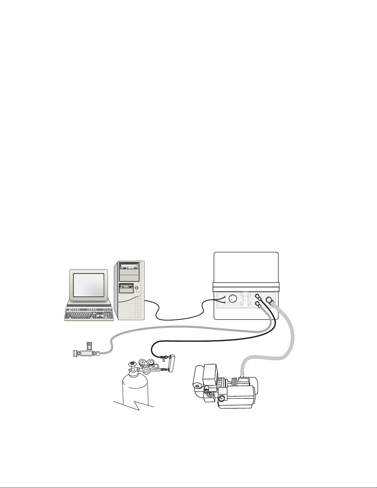
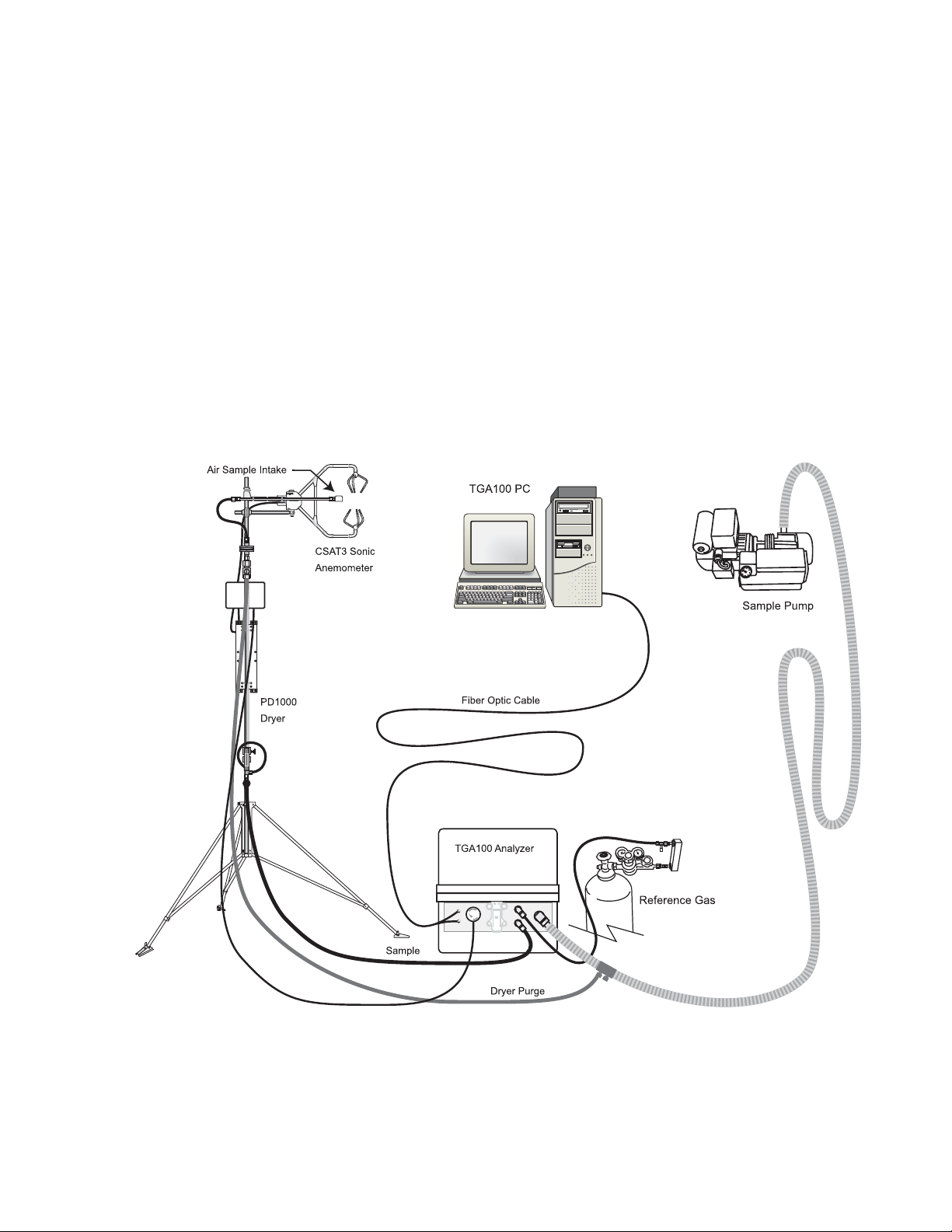
1.1 System Components

Figure 1-1 These system components include:

illustrates the main system components as well as additional equipment needed to operate the TGA100.

• TGA100 Analyzer: The analyzer optics and electronics, mounted in an insulated fiberglass enclosure.

• TGA100 PC: A desktop computer, supplied as part of the TGA100.

• Fiber optic cable (7737-L): Connects the TGA100 analyzer to the TGA100 PC.

• Sample Intake (15838 shown): Filters the air sample and controls its flow rate.

• Sample pump (RB0021-L shown): Pulls the air sample and reference gas through the analyzer at low pressure.

• Suction hose (7123): Connects the analyzer to the sample pump. Supplied with RB0021 sample pump.

• Reference gas: tank of reference gas, with pressure regulator (supplied by user).

• Reference gas connection (15837): Flow meter, needle valve, and tubing to connect the reference gas to the

analyzer.

TGA100 Analyzer

TGA100 PC

Fiber Optic Cable

Sample Intake

Reference Gas Connection

Reference Gas

Sample Pump

Figure 1-1. TGA100 System Components

Suction Hose

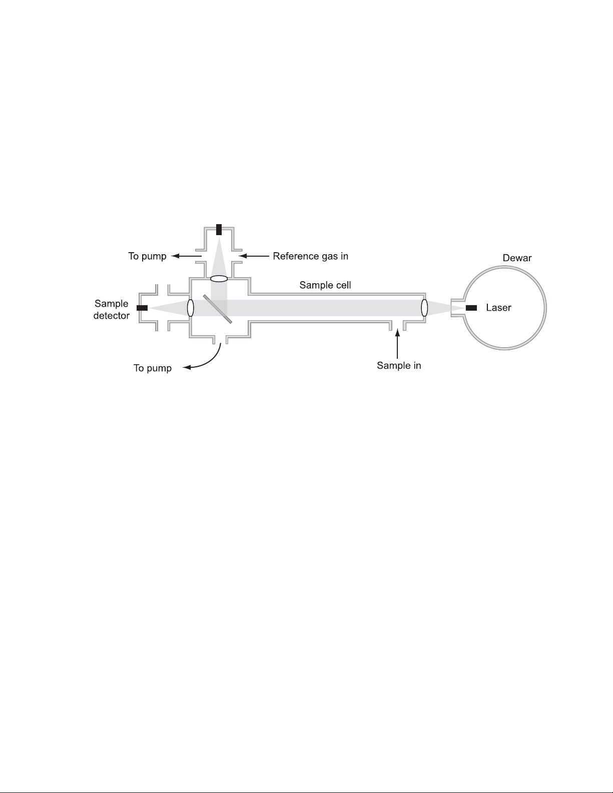
1.2 Theory of Operation

1.2.1 Optical System

The TGA100 optical system is shown schematically in . The optical source is a lead-salt tunable diode laser that operates between 80 and 140 K, depending on the individual laser. Two options are available to mount and cool the laser: the TGA100 LN2 Laser Dewar and the TGA100 Laser Cryocooler System. Both options include a laser mount that can accommodate one or two lasers. The LN2 Laser Dewar mounts inside the analyzer enclosure. It holds 10.4 liters of liquid nitrogen, and must be refilled twice per week. The Laser Cryocooler System uses a closed-cycle refrigeration system to cool the laser without liquid nitrogen. It includes a vacuum housing mounted inside the analyzer enclosure, an AC-powered compressor mounted outside the enclosure, and 3.1 m (10 ft) flexible gas transfer lines.

Reference detector

Figure 1-2

Figure 1-2. Schematic Diagram of TGA100 Optical System

The laser is simultaneously temperature and current controlled to produce a linear wavelength scan centered on a selected absorption line of the trace gas. The IR radiation from the laser is collimated and passed through a 1.5 m sample cell, where it is absorbed proportional to the concentration of the target gas. A beam splitter directs most of the energy through a focusing lens to the sample detector, and reflects a portion of the beam through a second focusing lens and a short reference cell to the reference detector. A prepared reference gas having a known concentration of the target gas flows through the reference cell. The reference signal provides a template for the spectral shape of the absorption line, allowing the concentration to be derived independent of the temperature or pressure of the sample gas or the spectral positions of the scan samples. The reference signal also provides feedback for a digital control algorithm to maintain the center of the spectral scan at the center of the absorption line. The simple optical design avoids the alignment problems associated with multiple-path absorption cells. The number of reflective surfaces is minimized to reduce errors caused by Fabry-Perot interference.

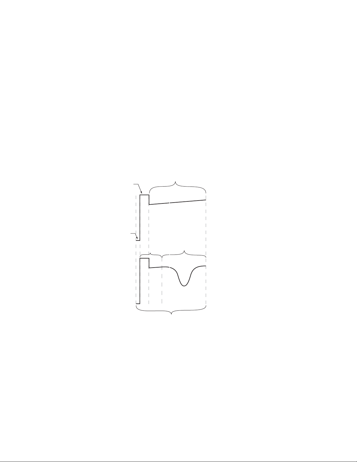
1.2.2 Laser Scan Sequence

The laser is operated using a scan sequence that includes three phases: the zero current phase, the high current phase, and the modulation phase, as illustrated in Figure 1-3. The modulation phase performs the actual spectral scan. During this phase the laser current is increased linearly over a small range (typically +/- 0.5 to 1 mA). The laser’s emission wavenumber depends on its current. Therefore the laser’s emission is scanned over a small range of frequencies (typically +/- 0.03 to 0.06 cm

-1

During the zero current phase, the laser current is set to a value below the laser’s emission threshold. “Zero” signifies the laser emits no optical power; it does not mean the current is zero. The zero current phase is used to measure the detector’s dark response, i.e., the response with no laser signal.

The reduced current during the zero phase dissipates less heat in the laser, causing it to cool slightly. The laser’s emission frequency depends on its temperature as well as its current. Therefore the temperature perturbation caused by reduced current during the zero phase introduces a perturbation in the laser’s emission frequency. During the high current phase the laser current is increased above its value during the modulation phase to replace the heat “lost” during the zero phase. This stabilizes the laser temperature quickly, minimizing the effect of the temperature perturbation. The entire scan sequence is repeated every 2 ms. Fifty consecutive scans are averaged and processed to give a concentration measurement every 100 ms (10 Hz sample rate).

Modulation Phase

High Current Phase

(Temperature

Stabilization)

(Spectral Scan)

Zero Current Phase

(Laser Off)

Omitted

Used in Calculation

2 ms

Figure 1-3. TGA100 Laser Scan Sequence

Laser Current

Detector Response

1.2.3 Concentration Calculation

The reference and sample detector signals are digitized and averaged over 50 consecutive scans. The average reference and sample scans are then corrected for detector offset and nonlinearity, and converted to absorbance. A linear regression of sample absorbance vs. reference absorbance gives the ratio of sample absorbance to reference absorbance. The assumption that temperature and pressure are the same for the sample and reference gases is fundamental to the design of the TGA100. It allows the concentration of the sample, C

Where C

= concentration of reference gas, ppm

= length of the short reference cell, cm

= length of the short sample cell, cm

= length of the long sample cell, cm

, to be calculated by:

))()((

DLC

)1(

DLL

−+

D = ratio of sample to reference absorbance

1.3 Trace Gas Species Selection

The TGA100 can measure gases with absorption lines in the 3 to 10 micron range, by selecting appropriate lasers, detectors, and reference gas. Lead-salt tunable diode lasers have a limited tuning range, typically 1 to 3 cm

-1

within a continuous tuning mode. In some cases more than one gas can be measured with the same laser, but usually each gas requires its own laser. The laser dewar has two laser positions available (four with an optional second laser mount), allowing selection of up to four different species by rotating the dewar, installing the corresponding cable, and performing a simple optical realignment.

The standard detectors used in the TGA100 are Peltier cooled, and operate at wavelengths up to 5 microns. These detectors are used for most gases of interest, including nitrous oxide (N Some gases, such as ammonia (NH

), have the strongest absorption lines at longer wavelengths, and require the

O), methane (CH4), and carbon dioxide (CO2).

optional long wavelength, liquid nitrogen-cooled detectors. These detectors operate to wavelengths beyond 10 microns. They require filling with liquid nitrogen once each day.

1.4 Dual Ramp Mode

The TGA100 can be configured to measure two gases simultaneously by alternating the spectral scan wavelength between two nearby lines. This technique requires that the two absorption lines be very close together (within about 1

-1

), so it can be used only in very specific cases. The dual ramp mode is used to measure isotope ratios in carbon

cm dioxide or water by tuning each ramp to a different isotopomer.

The dual ramp mode may also be used to measure some other pairs of gases, such as carbon monoxide and nitrous oxide, or nitrous oxide and methane, but the measurement noise will be higher than if a single gas is measured. For measurements of a single gas, the laser wavelength is chosen for the strongest absorption lines of that gas. Choosing a laser that can measure two gases simultaneously involves a compromise. Weaker absorption lines must be used in order to find a line for each gas within the laser’s narrow tuning range.

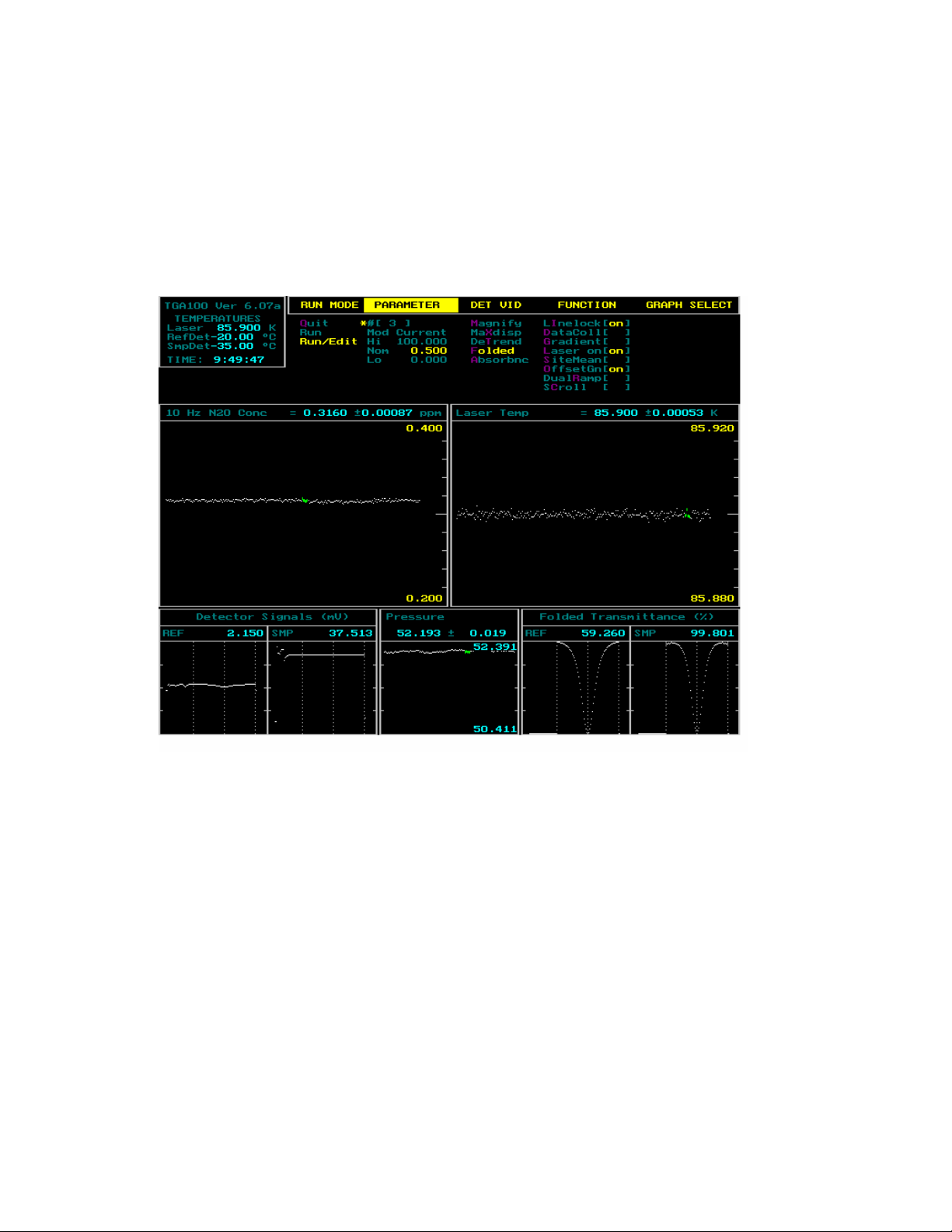
1.5 User Interface

The TGA100 includes a computer that provides the user interface. It displays the data in real time, allows the user to modify control parameters, and saves data to the hard disk. The real time graphics screen is presented in . In

Figure 1-4 the upper left corner is a box which displays the TGA software version, the laser and detector temperatures, and the time. Beneath the time and temperature display is a blank area used for information and error message display. The rest of the top of the screen has five menu columns: run mode, dynamic parameters, detector video, special function enable/disable, and graph selections.

Figure 1-4. Real Time Graphics Screen

In the middle of the screen are graph 1 and graph 2, used to display certain user-selectable variables. This example shows N

Graph 3 is located at the bottom-center of the screen, and is also used to display user-selected variables. In this example graph 3 shows the sample cell pressure.

At the bottom left corner of the screen are two high speed graphic windows that show the raw reference (REF) detector signal and the raw sample (SMP) detector signal, scaled to match the analog-to-digital converter (ADC) input range.

At the bottom right corner of the screen are two more high speed graphic windows that display processed reference and sample signals. The user may select the type of data to display in these windows using the Detector Video menu or the Quick Keys. The number displayed at the top of these windows is either the transmittance or the absorbance of the center of the spectral scan, depending on the display mode selected. All four of the high-speed graphic windows have three vertical dashed lines. These lines show the center of the spectral scan and the range of data actually used to calculate concentration.

O concentration in graph 2 and laser temperature in graph 2.

1.6 Micrometeorological Applications

The TGA100 is ideally suited to measure fluxes of trace gases using micrometeorological techniques. In addition to its rugged design that allows it to operate reliably in the field with minimal protection from the environment, it also incorporates several hardware and software features to facilitate these measurements.

1.6.1 Eddy Covariance

The TGA100's sample rate, frequency response, sensitivity and selectivity are optimized for measuring trace gas fluxes using the eddy covariance (EC) method. It is designed to collect three-dimensional wind data from a CSAT3 sonic anemometer while synchronously measuring trace gas concentration. Figure 1-5 illustrates a typical EC application. The sonic anemometer and air sample intake are mounted on the measurement mast. Tubing connects the air sample intake to the inlet of a PD1000 sample air dryer, which filters and dries the air sample. A needle valve at the outlet of the PD1000 sets the sample flow rate, typically to approximately 15 slpm. The TGA100 analyzer is located near the base of the measurement mast to minimize the length of sample tubing. This avoids the attenuation of high frequencies in the concentration data that can be caused by excessive tubing length. The TGA100 PC requires shelter from the environment, but can be located up to 500 m (1650 ft) away from the TGA100 analyzer, connected by fiber optic cable. The sample pump requires minimal shelter and can be located up to 90 m (300 ft) away from the analyzer, connected by the suction hose. The CSAT3 connects to the TGA analyzer by way of a TL925 serial interface module, which can be mounted inside the analyzer enclosure for protection from the environment.

CSAT3 Cable

Figure 1-5. Example Eddy Covariance Flux Application

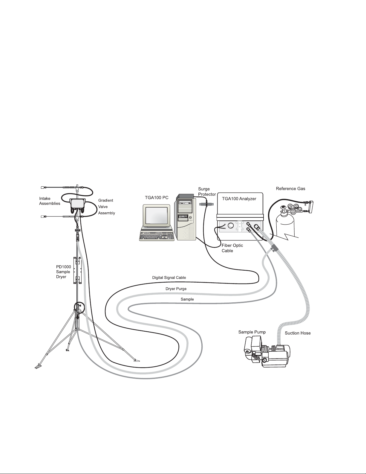
1.6.2 Flux Gradient

The TGA100 also supports the measurement of trace gas fluxes by the gradient method. The TGA100 automatically controls gradient switching valves and computes the mean concentration at each of the two intake heights. Timing parameters are entered by the user to control the gradient valves, typically switching between intakes every 5 to 20 s. The results are displayed on the TGA100 PC in real-time and stored on the hard disk.

Figure 1-6 measurement mast. Tubing connects each intake assembly to a gradient valve assembly that selects one of the intakes at a time. The air sample from the selected intake flows through the PD1000 sample air dryer, which filters and dries the air sample. A needle valve at the outlet of the PD1000 sets the sample flow rate, typically 5 to 10 slpm. Tubing connects the outlet of the dryer to the TGA100 analyzer, which may be located 200 m (650 ft) or more away. The TGA100 PC requires shelter from the environment, and can be located up to 500 m (1650 ft) away from the TGA100 analyzer, connected by fiber optic cable. However, for gradient applications the analyzer is normally positioned away from the intake mast, and the PC is placed near the analyzer for convenience. The sample pump requires minimal shelter and can be located up to 90 m (300 ft) away from the analyzer, connected by 1” ID suction hose.

This example shows a gradient flux measurement at a single site. However, the TGA100 can also support flux gradient measurements at multiple sites by installing intake assemblies, a gradient valve assembly, and a sample dryer at each site, and a site selection system near the analyzer. The site selection system connects one site at a time to the analyzer. The TGA100 controls the site selection system using timing parameters supplied by the user. Normally each site is measured for 15 to 30 min before switching to the next site.

illustrates a typical gradient application. Two intake assemblies are mounted at different heights on the

Figure 1-6. Example Gradient Flux Application

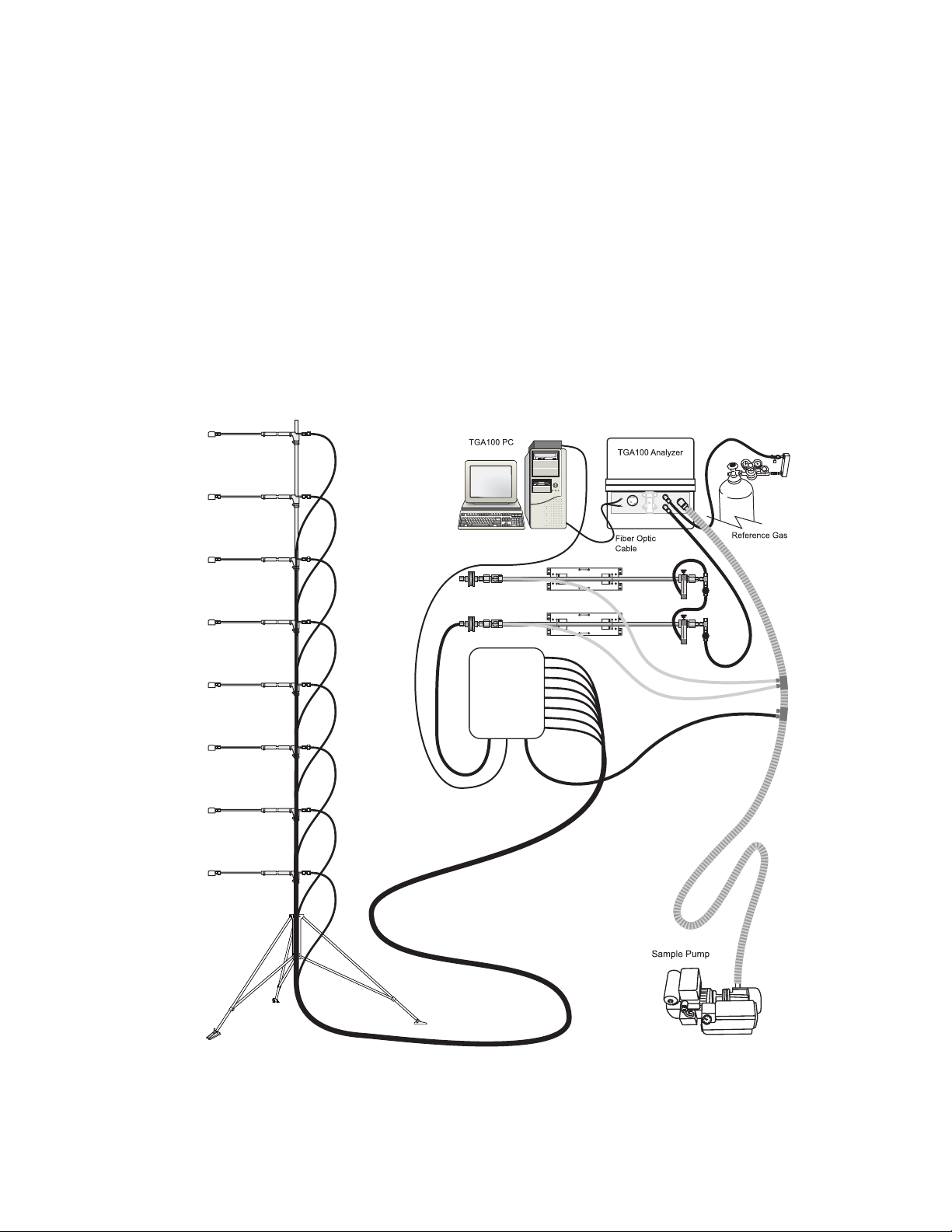
1.6.3 Site Means

The TGA100’s site means sampling mode is similar to the flux gradient mode in that it controls switching valves and calculates mean concentrations for each intake. The difference between the two sampling modes is that the gradient mode considers the sample intakes in pairs, switching several times between an upper and lower intake before moving to another site, but the site means mode considers all of the intakes as one group. It cycles through all of the intakes in sequence (up to 18 sites are supported). Applications for the site means mode include concentration profile measurements and trace gas flux measurements using the mass balance technique.

Figure 1-7

illustrates an eight-level vertical profile using the TGA100 site means mode. The eight intake assemblies are arranged vertically on a single measurement tower. These intake assemblies include a filter to remove particulates and a critical flow orifice to set the sample flow (typically less than 1 slpm). A separate tube connects each intake assembly to the site selection system, which selects one of the intakes at a time. All of the unselected intakes are connected through the bypass tube to the sample pump suction hose, keeping air flow at all times in all intake tubes. The flow from the selected intake goes through a sample air dryer to the TGA100 analyzer. A second dryer is used to provide dry air to purge the sample dryer.

Sample

Intakes

Digital Control Cable

Site Selection Sampling

Sample

System

Purge Dryer

Sample Dryer

Sample

Dryer Purge

Bypass

Figure 1-7. Example Profile Application

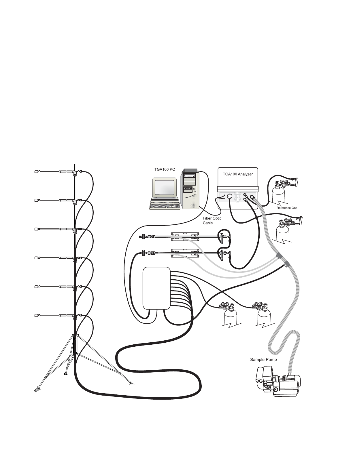
1.6.4 Absolute Concentration / Isotope Ratio Measurements

The TGA100 can be configured for highly accurate measurements of trace gas concentrations by performing frequent calibration. The TGA100 has a small offset error caused by optical interference. This offset error changes slowly over time, with a standard deviation roughly equal to the short-term noise. Offset errors have little effect on flux measurements by either the gradient or eddy covariance technique, but may be important in other applications. For measurements of absolute trace gas concentration, the offset error can be removed by switching between a nonabsorbing gas (e.g. nitrogen) and the sample, using the gradient mode of operation.

Applications such as isotopic ratio measurements require the highest possible accuracy. This is achieved using a frequent two-point calibration to correct for drift in the instrument gain and offset. High accuracy requires the flow rate for the calibration gases to be the same as for the sample air. Even though the sampling system can be designed so that calibration gases flow only when they are used, frequent calibration (every few minutes) consumes a large amount of calibration gas if high flow rates are used. The site means sampling mode is normally used because it works well at low flow rates.

Figure 1-8

illustrates a typical CO two intakes connected to calibration tanks. A tank of nitrogen or CO purge the air gap between the laser dewar and sample cell. This purge is required for CO because of the high ambient concentration of CO

isotope application. It is similar to the site means example above, but it also includes

-free air is also shown connected to the analyzer to

isotope measurements

and the need for high accuracy.

Sample

Intakes

Digital Control Cable

Sample

Site Selection Sampling System

Purge Dryer

Sample Dryer

Purge

Sample

Dryer Purge

Bypass

Calibration tanks

Figure 1-8. Example CO2 Isotope Application

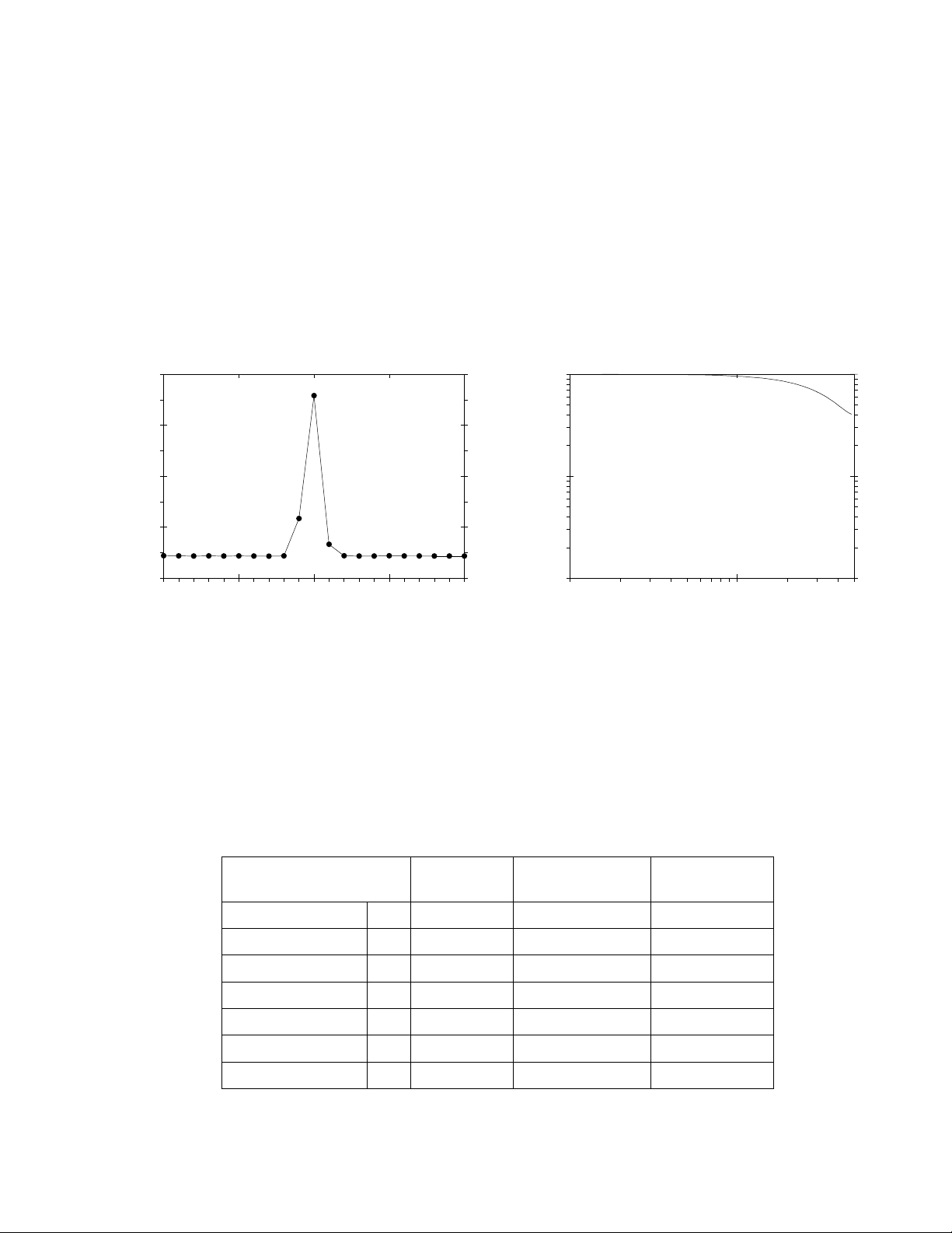
1.7 Specifications

1.7.1 Measurement Specifications

Sample Rate: 10 Hz

Averaging Period: 0.1 sec

Sample cell volume: 480 ml

Frequency Response (@ 4.8 liter/sec actual flow rate): 3 Hz

The TGA100 frequency response is determined by the averaging time (0.1 s) and the time for a new sample to fill the sample cell. The frequency response was measured at 14.4 slpm flow rate and 50 mbar sample pressure (4.8 actual l/s) by injecting 1 µl of N

O into the sample stream. The resulting time series and frequency response graphs are shown in

. Figure 1-9

Concentration (ppmv)

0.0

0.5

1.0

Time (sec)

1.5

2.0

0.1

Frequency Response

0.01

0.1

Frequency (Hz)

Figure 1-9. TGA100 Impulse Response (left) and Frequency Response (right)

The typical 10 Hz concentration measurement noise, given in , is calculated as the square root of the Allan variance with no averaging (i.e. the two-sample standard deviation. This is comparable to the standard deviation of the 10 Hz samples calculated over a relatively short time (10 s). The typical 30-minute average gradient resolution is given as the standard deviation of the difference between two intakes, averaged over 30 minutes, assuming typical valve switching parameters.

Table 1

Table 1. Typical Concentration Measurement Noise

Gas Wave number

(cm

-1

)

10 Hz Noise

(ppbv)

Nitrous Oxide N2O 2208.575 1.5 30

Methane CH4 3017.711 7 140

Ammonia NH3 1065.56 6 200

Carbon Monoxide CO 2176.284 3 60

Nitric Oxide NO 1900.08 13 260

Nitrogen Dioxide NO2 1630.33 3 60

Sulfur Dioxide SO2 1366.60 25 500

30-min Gradient

Resolution (pptv)

Typical performance for isotope ratio measurements is given in delta notation. For example, the δ by:



=−×





1 1000

VPDB

C for CO2 is given

where R

is the ratio of the isotopomer concentrations measured by the TGA100 (13CO2/12CO2) and R

standard isotope ratio (

13C/12

C). δ13C is reported in parts per thousand (per mil or ‰). The 10 Hz noise is the square

VPDB

is the

root of the Allan variance with no averaging. The calibrated noise assumes a typical sampling scenario: two air sample intakes and two calibration samples measured in a 1 minute cycle. It is given as the standard deviation of the calibrated air sample measurements.

Table 2. Typical Isotope Ratio Measurement Noise

Gas Isotope Ratio Wavenumber (cm-1) 10 Hz Noise (‰) Calibrated Noise (‰)

δ13C 2293.881, 2294.481 0.5 0.1 Carbon

Dioxide

1.7.2 Physical Specifications

Analyzer

Length: 211 cm (83 in)

Width: 47 cm(18.5 in)

Height: 55 cm (21.5 in)

Weight: 74.5 kg (164 lb)

Optional Cryocooler Compressor

Length: 31 cm (12 in)

Width: 45 cm (18 in)

Height: 38 cm (15 in)

Weight: 32 kg (71 lb)

Power Requirements

Analyzer: 90-264 Vac, 47-63 Hz, 50 W (max) 30 W (typical)

Optional Heater: 90-264 Vac, 47-63 Hz, 150 W (max)

PC: 115/230 Vac, 50/60 Hz, 150 W

Optional Cryocooler Compressor: 100, 120, 220, or 240 Vac, 50/60 Hz, 500 W

Optional sample pump (RB0021-L): 115 Vac, 60 Hz, 950 W (other power options are available)

O 2308.225, 2308.416 2.5 0.5

δ18O 1500.546, 1501.188 2 0.5 Water

δD 1501.813, 1501.846 10 2.5

2 INSTALLATION

The basic components required to operate the TGA100 are shown in Fi . Other components, such as a sample air dryer, valves to switch between multiple intakes, calibration gases, etc. may also be required, depending on the user’s application. These optional components will be discussed in other sections.

gure 2-1

TGA100 Analyzer

TGA100 PC

Fiber Optic Cable

Reference Gas Connection

Suction Hose

Sample Intake

Reference Gas

Sample Pump

Figure 2-1. Basic Components Required for TGA100 Operation

2.1 Analyzer Installation

The TGA100 analyzer (the optics and electronics) is housed in an insulated fiberglass enclosure that allows it to operate in the open environment. However, if a tent or other shelter is not available, the optional TGA Temperature Controller and TGA Insulated Enclosure Cover are recommended. The analyzer must be placed on a stable surface. If placed on uneven ground, wooden blocks or other supports can be used under the two pairs of rubber feet near the ends of the enclosure. Older enclosures have a third pair of rubber feet in the center, but should be placed on blocks so that only the four feet on the ends are used.

The analyzer should be connected to other system components as follows:

1) Connect the vacuum exhaust outlet of the analyzer to the sample pump using 1" ID exhaust hose and hose clamps.

The sample pump must be able to pull the required flow rate at 75 mbar or less. The actual flow rate and pressure required will depend on the application. The RB0021, available from Campbell Scientific, has a capacity of 18 slpm at 50 mbar (15 slpm with 50 Hz power), and is adequate for most applications.

2) Connect the reference gas supply to the reference gas inlet on the end of the analyzer. The reference gas supply

should have an appropriate regulator, flow meter, and needle valve to supply approximately 10 ml/min. See section

4.1.2 for more details on the reference gas.

3) Connect the sample intake to the sample gas inlet. The sample intake should be filtered to remove particulates (10

µm maximum pore size) and should have an appropriate needle valve or fixed orifice to control the sample gas flow and pressure.

4) Connect power. For older units, connect a user-supplied, regulated 12 Vdc supply with at least 5 ampere capacity

to the system enclosure POWER IN connector. Use the supplied external cable (CSI PN 7987) with the red wire connected to +12 volts and the black wire to ground return. Newer units are supplied with an internal, universalinput power supply. Connect the power supply to AC power (100-240 Vac, 47-63 Hz, 1.6 A). The use of an appropriate surge protector is highly recommended. However, unless the entire system can be powered from an uninterruptible power supply (UPS), including the sample pump, this electronics power supply should not be connected to a UPS. This will allow the system to initiate an automatic restart if power is temporarily interrupted.

5) For newer units equipped with a TGAHEAT temperature controller, set the temperature by inserting a small

screwdriver into the Temperature Setting hole in the TGAHEAT module in the analyzer electronics. Rotate the screw to the desired temperature (10 to 50 °C). Connect its power supply to AC power (85-132 Vac, 3.2 A, or 170264 Vac, 1.8 A, at 47-63 Hz). The use of an appropriate surge protector and a UPS is highly recommended, to help the automatic restart sequence find the correct absorption line when power is restored.

6) For isotope ratio applications, the short sample cell and the air gap between the dewar and lens and the short

sample cell should be purged to prevent absorption by ambient air, as discussed in section 4.1.4.

More details on configuring the TGA100 to measure a specific trace gas can be found in section 4.1.

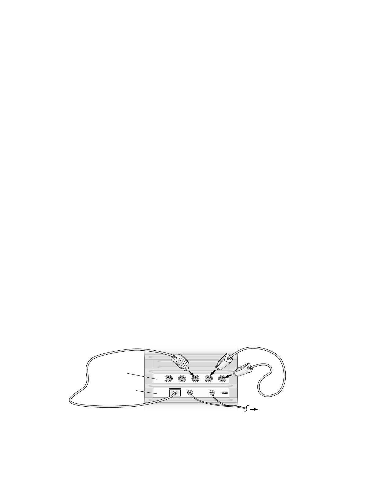
2.2 TGA100 PC Installation

The TGA100 includes a standard desktop personal computer (PC) to provide the user interface; controlling the analyzer, and calculating, displaying, and storing data in real time. The TGA PC must be protected from the weather. The TGA PC may be located up to 1650 ft. (500 m) from the TGA100 analyzer, determined by the length of the fiber optic interconnect cable. To install the TGA PC:

1) Connect the monitor, keyboard, and mouse (if applicable) to the TGA100 PC.

2) Connect the PC and monitor to AC power. The PC and monitor should operate with any AC power (115/230 Vac,

50/60 Hz). However, if this is an initial installation, check the voltage selector on the PC for proper setting (115/230 Vac). The use of an appropriate surge protector and uninterruptible power supply (UPS) is highly recommended for the PC. The monitor should be powered with a surge suppressor only.

3) Use the fiber optic cable (CSI PN 7737) to connect the analyzer to the link adapter card in the TGA PC.

4) Connect the link adapter card in the TGA PC to the transputer card in the PC. There are two versions of the

transputer card, with a different style connector and cable.

a) For older TGA100s, connect the 18-inch cable with one 8-pin mini-din connector and one RJ45 telephone-

type connector (CSI PN 10699) between the link adapter board and the third (center) connector on the PC transputer board. Connect the cable with two 8-pin mini-din connectors (CSI PN 7917) between the two adjacent connectors on the transputer which are farthest from the PC’s mother board, as shown in Figure 2-2.

Single Stand-Alone System

Transputer Board

TLINK

Link Adapter

OUT

Figure 2-2. Link Adapter Cable Connections

Fiber optic out to TGA

b) Newer TGAs have a transputer board with a single “D” connector, and a single cable assembly to make this

connection.

5) Connect the 7996 I/O terminal board (if needed) to the optional 7996 I/O board in the TGA PC.

2.3 Routine Operation

Once the TGA100 has been set up, it should be checked periodically to verify proper operation, download data files, and fill the laser dewar with liquid nitrogen, if necessary. This section gives suggestions for routine operating procedures.

2.3.1 Startup Procedure

This section describes the routine startup procedure for the TGA100. It assumes the TGA100 has been operational and is being restarted after a routine shutdown. This section is not intended as a full explanation of the operation of the TGA100; it is a brief checklist, with cross references to other sections of the manual which provide more detail.

1) Verify the laser dewar vacuum integrity. See section 8.1.

2) Cool the laser dewar. See section 8.1. Do not turn the laser on until it is cold. To run the TGA program with the

laser warm, disable the laser at the main menu before proceeding to the real time screen.

3) If the TGA100 is equipped with the optional liquid nitrogen-cooled detectors (used for long wavelength operation),

cool the detectors with liquid nitrogen. If the TGA100 is equipped with the standard thermoelectric-cooled detectors, they will be cooled automatically.

4) Start the sample vacuum pump.

5) Turn on the reference gas. A flow rate of approximately 10 ml/min is recommended.

6) Turn on the air gap purge gas, if required (isotope ratio measurements). A flow rate of approximately 10 ml/min is

recommended.

7) Turn on calibration gas supplies, if applicable.

8) Power up the TGA analyzer.

9) Power up the TGA PC, start the TGA program, and start real time operation (see section 3.2).

10) Verify the TGA pressure is consistent with the previous operation of the TGA. The sample pump capacity and the

total flow at the pump determine the pressure. Therefore, if the pressure has changed, it may indicate a problem in the plumbing.

11) Wait for the laser temperature to stabilize.

12) Verify the correct absorption line is being scanned. See section 0.

13) Initiate the line lock algorithm to bring the absorption line to the center of the spectral scan.

14) For dual ramp applications, start the ramp B line lock.

15) Verify the detector signals are consistent with previous operation of the TGA. If they have changed, check the

operational parameters (see section 4.4.)

16) Verify the reference transmittance at the center of the absorption line is consistent with previous operation of the

TGA. This transmittance is dependent on which absorption line is selected, the concentration in the reference cell, the pressure in the reference cell, and the laser performance. A significant change indicates a problem.

17) Check the concentration standard deviation to verify proper performance.

The TGA100 is now fully functional. Other features such as Site Means or Gradient Mode, communication with other devices, or data collection may now be started.

2.3.2 Shutdown Procedure

This section describes the routine shutdown procedure for the TGA100. It assumes the TGA100 is operating in the Real Time mode.

1) If data collection is on, turn it off.

2) If Site Means or Gradient mode is on, turn it off.

3) Exit the Real Time display mode.

4) Exit the TGA program.

5) Shut off power to the TGA PC and monitor.

6) Shut off the TGA sample pump.

7) Shut off power to the TGA enclosure.

8) Shut off the reference gas supply.

9) Shut off the air gap purge supply, if applicable.

10) Shut off calibration gas supplies, if applicable.

If the TGA100 is not to be operated for an extended period, allow the laser to warm up. If the laser is to be operated again in the near future, it is recommended to keep the laser cold to avoid temperature cycling the laser.

2.3.3 System Checks

The TGA100 is often used for long term continuous measurements. It is necessary to periodically check the status of the system, perform routine maintenance, and transfer data for offline analysis.

1) Look for a message printed in red above graph 1 indicating the system has restarted. If it has restarted, it is

important to verify it is on the correct absorption line.

2) Verify concentration data collection and site means or gradient mode are ON (if used).

3) Verify the line lock is ON. If the TGA100 is in dual ramp mode, also verify the Ramp B line lock is ON.

4) Note the DC current (it is recommended that this be recorded in a log book). Compare it to the expected value to

verify the laser is still operating on the desired absorption line. If the TGA100 is in dual ramp mode, also note the Ramp B offset.

5) Verify that the concentration and concentration noise are as expected. If the TGA100 is in dual ramp mode, also

verify the Ramp B concentration and noise.

6) Note the sample pressure (it is recommended that this be recorded in a log book). Compare this to the previous

values. The pressure will decrease over time as the sample intake filter(s) becomes plugged.

7) Note the laser heater voltage (it is recommended that this be recorded in a log book). Compare this to the previous

values. The vacuum inside the laser dewar will gradually degrade. This degradation reduces the thermal isolation between the outer wall of the laser dewar and the laser itself. Over time, as more heat is transferred to the laser by the degraded vacuum, less heat is needed to maintain the laser at the set temperature, and the laser heater voltage will gradually decrease. Therefore, monitoring the laser heater voltage may give an indication of when it is time to evacuate the dewar. This is especially important for cryocooler systems and for lasers that must operate at very cold temperatures.

8) Exit the real time screen and stop the TGA program.

9) Download data. The details will vary from one system to another. The data can then be transferred by copying to

CD ROM, Zip disk, etc. Check the files to verify the expected files are present.

10) As soon as the data are downloaded, restart the TGA program and go to the real time screen. This will let the laser

and detector temperatures stabilize as the next steps are completed.

11) If needed, fill the laser dewar with liquid nitrogen. If the TGA is equipped with liquid nitrogen cooled detectors,

fill these as needed.

12) Check the reference gas tank and regulator pressure. Check other tanks (air gap purge, calibration, etc.) as needed.

13) If a change in the sample pressure indicates the sample intake filter(s) must be changed, shut off the sample

vacuum pump. Wait for the pressure to reach ambient, and then replace the filter element(s). Restart the sample vacuum pump.

14) Restart the TGA (see section 2.3.1).

3 TGA SOFTWARE

3.1 General

The TGA software runs on the TGA PC. It provides the user interface to the TGA100, allowing the user to view the operation of the TGA, set parameters, and collect data. The TGA program actually is a set of three programs that run concurrently on three computers, communicating in real time. The first computer is the TGA PC itself. It runs the user interface and data storage functions of the TGA software. The second computer is the 9030 CPU module mounted in the TGA electronics chassis in the TGA enclosure. This computer controls the detector temperatures, the laser temperature and current, performs the measurements, and sends the data to the third computer, which is the transputer board mounted in the TGA PC. This third computer acts as an interface between the other two, and performs most of the calculations required to compute the concentration. When two or more TGA100s are linked together in the master/slave configuration, the transputer board also provides the communication link between them.

Normally it is not important for the user to be aware of the three computers and the roles they play. It is sufficient to know that the TGA program runs on the TGA PC, the transputer board must be installed in the PC, and the transputer board must be connected to the TGA enclosure through the link adapter and the fiber optic cable. However this information may be useful in troubleshooting problems.

The following sections discuss the details of the TGA software.

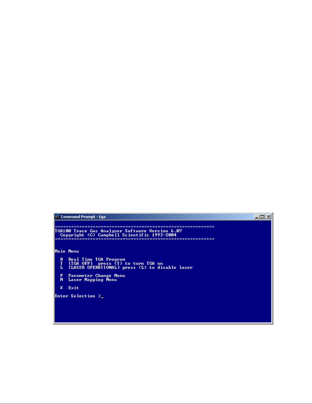
3.2 Startup

The TGA program is a DOS mode program. Although it may be run under the Windows operating system, it will run more reliably when the TGA PC is started in DOS mode.

The executable file is TGA.EXE, normally installed in the C:\TGA directory. The program is started by setting the default path to C:\TGA and entering the command <TGA>. The TGA program starts at the main menu.

3.3 Main Menu

When the TGA program is started, the main menu is displayed as shown below:

Figure 3-1. Main Menu

The functions available at the main menu are described below.

R) Real Time TGA Program

Turns the TGA on and displays the real time screen. This is the normal operating mode. See section 3.4 for

additional information.

T) TGA on/off

Toggles the TGA on or off. When the TGA is on, all current and temperature controls are active and

concentration calculations are being made, but the real time screen is not displayed, and no data are saved to the hard disk.

L) Laser on/off

Toggles the laser on or off. The laser must be on during normal operation. The laser may be disabled to

operate the TGA100 without driving the laser. For example, the laser temperature may be monitored during the initial cool down by disabling the laser at the main menu and then entering the real time screen.

P) Parameter Change Menu

Displays submenus for changing parameters. See section 3.5 for additional information.

M) Laser Mapping Menu

Displays the mapping submenu to be used to characterize a laser. See section 4.3 for additional information.

X) Exit

Exit TGA program.

3.4 Real Time Screen

The Real Time Screen is entered by pressing “R” at the main menu (see section 0.) This is the normal operating mode for the TGA100. Concentration data can be displayed or saved only while in the real time mode.

3.4.1 Screen Layout

The real time graphics screen is presented in . In the upper left corner is a box which displays the TGA software version, the laser and detector temperatures, and the time. Beneath the time and temperature display is a blank area used for information and error message display. The rest of the top of the screen has five menu columns: run mode, dynamic parameters, detector video, special function enable/disable, and graph selections.

Figure 3-2

Figure 3-2. Example Real Time Screen

In the middle of the screen are graph 1 and graph 2, used to display certain user-selectable variables. The horizontal time step is 0.1 sec and the horizontal width is 280 pixels or 28 seconds. The title bar at the top of each window shows the variable name, the floating point value and its standard deviation, and the units. The maximum and minimum display limits are shown in the upper right and lower right corners.

Graph 3 is located at the bottom-center of the screen, and is used to display user-selected variables. The graph 3 window is 150 pixels wide or 15 seconds. Graph 3 also has the variable name, value, standard deviation, and display limits noted on the graph.

3.4.2 Navigating and Editing

The <left/right arrow> keys are used to cycle through the following menus: RUN MODE, PARAMETER, DET VID, FUNCTION, GRAPH 1, GRAPH 2, GRAPH 3, DETECTORS, Graph 1 display scale, and Graph 2 display scale. The heading for the current menu is highlighted. The active option within each menu is also highlighted. The <up/down arrow> keys are used to select a specific option (marked with an asterisk “*”) within the selected menu and the <Enter> key is used to activate the option. To adjust the value of a numeric field (dynamic parameter or graph display limit), use the <Home End> keys for coarse adjustments, <Page Up Page Down> keys for normal adjustments, the <+-> keys for fine adjustments, and the </ *> keys for very fine adjustments. Number pad and keyboard give the same results. Each field is described below.

3.4.3 Run Mode

The first menu in the Real Time screen controls the run mode. The options are Quit, Run, or Run/Edit.

Upon entering the Real Time Screen, the run mode is Run/Edit which enables the display and parameters to be edited using either cursor motion or the Quick keys.

Once operating conditions have been established, the Run mode may be selected to disable the Quick keys and editing capability. This may be useful to avoid problems caused by pressing a key inadvertently. In Run mode, the user may adjust the display, but can not adjust any of the dynamic parameters are operating functions.

Quit stops real time operation and returns program control to the main menu. The hardware continues to control and monitor temperatures but any open data storage files are closed. The <escape> key has the same effect as selecting Quit.

3.4.4 Dynamic Parameters

The next menu column, labeled “PARAMETERS”, provides access to the dynamic parameters, i.e. those that may be changed in real time. The <up/down arrow> keys are used to scroll through the list of dynamic parameters (listed in Table 3 <Home End PgUp PgDn + - / *> keys. Use the <Home End> keys for coarse adjustments, <Page Up Page Down> keys for normal adjustments, the <+ -> keys for fine adjustments, and the </ *> keys for very fine adjustments. Number pad and keyboard give the same results.

Some dynamic parameters may be controlled automatically. In this case, the value is displayed and updated in real time, and an “A” will appear to the right of the value. Changing the value of a dynamic parameter that is being controlled will disable the control function.

The dynamic parameters are a subset of the parameters stored in the parameter file and can also be edited through the parameter change menu (see section 3.5). Table 3 lists the dynamic parameters by the abbreviated name shown in the real time screen and gives the full parameter name shown in the parameter change menus (see section 3.5). Changes made to these parameters in the Real Time Screen are saved in the parameter file.

). If the Run/Edit mode is selected, the value of the selected dynamic parameter may be changed using the

Table 3. Dynamic Parameters

Abbreviated Name Units Full Parameter Name

1 Laser Temp K Laser operating temperature (K)

2 DC Current mA Laser DC current (mA)

3 Mod Current mA Laser Modulation current (mA)

4 High Current mA Laser High current offset (mA)

5 Zero Current mA Laser Zero current (mA)

6 SMP Gain -- Sample detector gain

7 SMP Offset -- Sample detector offset

8 SMP Det Temp ºC Sample detector operating temp (deg C)

9 REF Gain -- Sample detector gain

10 REF Offset -- Reference detector offset

11 REF Det Temp ºC Reference detector operating temp (deg C)

12 Std Dev Time sec Mean, StdDev time frame (sec)

13 Graph3 Range -- Graph 3 range

14 SMP Det Lin -- Sample detector linearity coeff

15* RampB Offset mA Ramp B offset current (mA)

16* RampB Mod mA Ramp B Modulation Current (mA)

17* RampB High mA Ramp B High current (mA)

18* SmpDetLin B -- Ramp B Smp detector linearity coeff

* Dynamic parameters 15 through 18 are available only in dual ramp mode.

3.4.5 Detector Video

This next menu column, labeled “DET VID”, is used to select the display mode of the processed detector data in the two bottom-right displays. The display mode may be selected either by pressing the corresponding Quick key or by highlighting the selection using the <up/down arrow> keys and pressing <enter>. Each option is discussed below.

Magnify displays the reference and sample transmittance, scaled to the maximum and minimum of the data used in

the concentration calculation (i.e., the data between the vertical dashed lines).

MaXdisp displays the reference and sample transmittance, scaled to the maximum and minimum of all of the data

(including the zero, high, and omitted data).

DeTrend display mode is similar to the Magnify display mode, but the data have been detrended by fitting a line to

the data and dividing by this line.

Folded display mode is similar to the Magnify display mode, but the data have been averaged with a reversed copy

of the data to make them symmetrical about the center of the spectral scan (the center vertical dashed line).

Absorbnc mode displays the absorbance of the (folded) data instead of the transmittance.

3.4.6 Functions

The FUNCTION menu allows the user to turn functions on or off, and displays their status. The functions are indicated as either on i.e. [on] or off i.e. [ ]. The functions may be toggled on/off either by pressing the Quick key or by highlighting the selection using the <up/down arrow> keys and pressing <enter>.

LInelock[ ] automatically adjusts the laser DC current to keep the reference absorption line minimum in the center

of the spectral scan. The line lock function must be on during normal operation.

DataColl[ ] turns 10 Hz data collection on or off. This function must be on to save the concentration data to a file.

Gradient[ ] turns gradient measurements on or off (see section 5.1).

Laser On[ ] turns the laser on or off. The laser must be on for normal operation.

SiteMean[ ] turns site means measurements on or off (see section 5.2).

OffsetGn[ ] turns automatic control of detector gains and offsets on or off. This function is normally on during

routine operation.

DualRamp[ ] turns dual ramp mode on or off.

SCroll [ ] toggles graphs 1 and 2 between scroll and retrace mode.

3.4.7 Graph Selections

This field is used to select the variable to be displayed in graphs 1, 2, 3, or the detector graphs. When this field is not selected, its heading reads “GRAPH SELECT” with a blank area below. When it is selected, its heading will read either “GRAPH 1”, “GRAPH 2”, “GRAPH 3”, or “DETECTORS” depending on which menu is selected using the left arrow or right arrow keys. The “DETECTORS” menu is available only if dual ramp mode is on. The options for the graph selected (1, 2, 3, or DETECTORS) will be displayed below the heading, and the border of the graph selected will be highlighted.

There are up to 65 options available for display in Graphs 1, 2 or 3. These options are displayed one page at a time, and the user may view the other options using the <up/down arrow> keys, the <PgUp, PgDown> keys, or the <Home/End> keys. Use the <up/down arrow> keys to scroll up and down one item at time. When the top or bottom of the list is reached, pressing the <up/down arrow> key one more time will display the next page of options. Pressing <PgUp, PgDown> keys will also display more options. The <Home/End> keys will move you to the beginning or the end of the list, respectively. The complete list of display options is found in Appendix A.

In dual ramp mode, the “DETECTORS” menu becomes available, allowing the user to select which ramp (A or B) is displayed in the detector signal graphs in the lower left corner of the real time screen and the transmittance graphs in the lower right corner. In single ramp mode, the average of ramps A and B is always displayed. describes the

Table 4

options available in the “DETECTORS” menu.

Table 4. Detector Graph Display Options

DETECTORS Description

Ramp A Ramp A, reference and sample detectors

Ramp B Ramp B, reference and sample detectors

Alt A&B Alternate between Ramp A and Ramp B, reference and sample detectors

RefDet A&B Reference detector, ramp A and B.

SmpDet A&B Sample detector, ramp A and B.

3.4.8 Graph Display Limits

The Y-axis limits for graphs 1, 2, and 3 are displayed in the upper right and lower right corners of each graph. These limits are set by the user for graphs 1 and 2 by moving the cursor (using the arrow keys) onto the limit to be changed, and then using the <Home End PgUp PgDn + - / *> keys to adjust the value, similar to the adjustment of the dynamic parameters. However, for setting graph limits, the step size corresponding to each set of keys depends on the difference between the limits. This adaptive step size allows for faster changes when the limits are far apart and gives finer control as the limits approach each other.

The Y-axis limits for graph 3 are set with a single parameter, the Graph 3 Range (dynamic parameter 13). This parameter sets the range of the graph, and this range is offset automatically if a measurement goes outside the graph range. The graph 3 range should be set high enough to avoid frequent automatic offsets.

The graph ranges can also be adjusted by using the quick keys <Alt-1>, <Alt-2>, and <Alt-3>. When the user types <Alt-1>, the graph 1 limits are set to the mean ± (50 times the standard deviation), using the most recent 64 data values (6.4 s). This usually gives reasonable values for the graph limits. Similarly, typing <Alt-2> adjusts graph 2, and typing <Alt-3> adjusts graph 3.

3.4.9 Quick Keys

Pressing a quick key calls its associated function directly, without moving the cursor. Most of the quick keys are associated with functions available in a real time screen, but some additional Quick Keys are available as well. Here is a summary of all of the Quick Keys.

Key Function

Table 5. Quick Key Summary

Alt-I

Turn line locking on/off for ramp A

Turn line locking on/off for ramp B. Available only when dual ramp mode is on.

Turn data collection on/off

Turn gradient mode on/off

Turns laser current on/off

Turn site mean mode on/off

Turn automatic control of detector gain and offset on/off

Turn dual ramp mode on/off

Toggle graphs 1 and 2 between scroll and retrace mode

Select Magnify mode for the reference and sample detector displays.

Select maXdisp mode for the reference and sample detector displays.

Select deTrended mode for the reference and sample detector displays.

Select Folded mode for the reference and sample detector displays.

Select Absorbance mode for the reference and sample detector displays.

Same as the QUIT mode or <escape>: it stops real time operation, closes data files, and returns to the main menu

Turn on or off the display of vertical grid lines in graph 1 and graph 2 that correspond to switching valve control. This mode is enabled by default, but the lines are displayed only if the site means mode or the gradient mode is active. See section 5.

AltZ

AltM

AltN

Alt1

Alt-2 Similar to <Alt-1>, for graph 2.

Alt-3 Similar to <Alt-1>, for graph 3.

AltC

Turn on/off printer output for the site means or gradient mode. When enabled, all information that is written to a site means or gradient file will also be written to a printer. This mode is disabled by default.

Start an automated sequence to optimize the value of the Laser Zero Current. See section 4.4.2.

Start an automated sequence to optimize the value of the Laser Modulation Current. See section 4.4.5.

Start an automated sequence to optimize the value of the Ramp B Laser Modulation Current. Available only when dual ramp mode is on. See section 4.4.5.

Adjust the graph 1 limits to the mean ± (50 times the standard deviation), using the most recent 64 data values (6.4 s).

If the header file is open, this key will print a message in the header file. The user may type in the message or press a function key to enter a previously defined message. See section 3.6.7 for a listing of the predefined messages.

3.5 Parameter Change Menu

The system parameters are stored in the file, TGAPARM.CFG, which is read when the program is loaded. TGAPARM.CFG is updated at the end of real time operation to maintain a current parameter set, and a new file MMDDHHMM.gas (gas is a parameter) is written when data collection is started, maintaining a history for future reference (see section 3.6.1).

The parameter change menu may be used to change system parameters. Upon entering <P> from the main menu, the user is presented with the following menu:

Figure 3-3. Parameter Change Menu

There are fourteen parameter screens, with similar types of parameters grouped together. These screens are organized as follows:

Parameter Change Menu Laser Detector Ramp B Concentration Calculation File Format File Output Selection Analog Output Valve Control Menu Gradient Mode Site Means Mode Miscellaneous Valve Control

Miscellaneous Menu

Serial Numbers Pressure Calculations Graph Setup Laser Map Temperature and Current

Parameter File Operations Menu

Save parameters to user-specified file Read user-specified parameter file Document parameters (create tgaparm.doc)

3.5.1 Standard Parameter Screens

Most of the parameter screens have three columns, containing the parameter name, value, and allowable range, as shown in Figure . The selected parameter value is highlighted and a corresponding prompt is displayed at the bottom of the screen. Use the <up/down arrow> keys to select the parameter to be edited. To change the selected parameter’s value, type the new value and press <enter> or the <up/down arrow> keys. To cancel a change while typing in a new value, press the <escape> key. To return to the main menu press the <escape> key.

Figure 3-4

Figure 3-4. Example Parameter Screen

3.5.2 File Output Selection Screen

The File Output Selection screen selects which data will be included in the 10 Hz data file. It has four columns, containing the on/off indicator ([X] to save data, or [ ] to skip), the description, the present value, and the units. The present value and units are displayed only if the TGA is on. An example of the File Output Selection screen is shown in Figure . To toggle whether the selected parameter should be saved or not, type <space>, <enter>, or ‘X’. Use the <up arrow / down arrow> to change the selected parameter, and to see more options, type <Pg Up>, <Pg Down>, or highlight “Prev Page” or “Next Page” and hit <enter>.

Figure 3-5

Figure 3-5. Example File Output Selection Screen

Some of the file output options are not available all the time. For example, if dual ramp mode is turned off, then no Ramp B data can be saved. The list of values that can be saved is the same as the list that can be displayed in the real time screen graphs (see section 3.4.7). For a list of file output options, see Appendix A.

The descriptions for user-defined parameters (analog inputs and other device data) can be edited. To edit these descriptions, select the row, press the <right arrow> key, and type in the new description.

3.5.3 Analog Output Screen

The Analog Output screen allows the user to configure the analog output channels (see section 0). Use the <up/down/right/left arrow> keys, or the <TAB> and <shift-TAB> keys to move to the field to be changed. To change which data will be output, highlight the desired channel, and type <enter>. A new menu will appear that will show the options available for output. These options are the same as for the real time graphs and for output to the 10 Hz data file, and are listed in Appendix A. Use the <up/down/right/left arrow> keys, the <Pg Up / Pg Down> keys, and the <TAB> and <shift-Tab> keys to select the desired option, and then hit the <enter> key.

If the TGA is running, the current value of the parameter and the corresponding analog output voltage will be displayed, as shown in . Figure 3-6

Figure 3-6. Example Analog Output Screen

3.5.4 Gradient and Site Means Screens

The Site Means and Gradient screens allow the user to edit valve switching parameters (see section 5). These screens are organized in rows and columns, with one row for each site, as shown in Figure 3-7. The user can navigate to each field using the <up/down/left/right arrow> keys, or the <TAB> and <shift-TAB> keys. Type the number and press <enter> or an arrow key to change a selected field.

Figure 3-7. Example Site Means Screen

3.6 TGA Files

The TGA system uses and creates several different types of files. Many of the files are automatically named based on the date and time the file is created. For example, if the file were created on 29 July, at 3:45 PM, the filename would be

07291545.xxx. This is referred to generically in this manual as MMDDHHMM.xxx. The file extension will be DAT, MIN, SM, DC, or HDR for concentration, housekeeping, site mean, gradient, and header files, respectively. These files are stored in the path defined in the DOS environment variable TGADATA. The default data location is c:\tgadata. If the “European date format” parameter is set, the format of the file names will be DDMMHHMM.xxx.

3.6.1 Parameter Files

Parameter files are ASCII (plain text) files which store all of the parameters necessary to run the TGA program. The default location of all parameter files is c:\tgaparm, but can be changed to a user-specified location by modifying the “set TGAPARM=C:\TGAPARM” statement in the autoexec.bat file. The file TGAPARM.CFG contains the working set of parameters which the program automatically loads at startup and updates at exit.

In addition to the working parameter file, each time a concentration file, gradient file, or site mean file is opened, a parameter file called MMDDHHMM.gas is saved for future reference. The file extension “gas” is the "Gas Mnemonic" parameter, set in the "Concentration Calculations" screen. It is normally chosen to describe the gas being measured, e.g. CH4 or N2O.

Three functions are available at the Parameter File Operations screen to help the user manage parameter files:

S Save parameters to user-specified file

R Read user-specified parameter file

D Document parameters (create tgaparm.doc file)

The Save and Read functions allow the user to store and recall a particular TGA setup. The Document function creates file tgaparm.doc, which documents the parameters in a format very similar to the parameter editing screens.

It is very important that the working parameter file, tgaparm.cfg, is not deleted or corrupted. If there is no valid parameter file when the TGA program is started, a set of default parameters will be used. These defaults are designed to be non-operational, to protect the laser, and to make it obvious to the user that correct parameters are not in use. If this happens, restore the parameters, either by reading in a valid parameter file, or by entering new parameters in the parameter editing screens.

Most of the parameters can be edited using the parameter change screens described in section 3.5, and a subset can also be edited from the real time screen, as described in section 3.4.4. A complete list of the contents of the parameter file (in the tgaparm.doc file format) is given in Appendix A.

3.6.2 10 Hz Concentration Data Files

Data are saved by enabling the data collection function (by pressing the <D> Quick key) from the real time screen. This creates a file called MMDDHHMM.DAT. Normally data are written to the same file until data collection is shut off. Optionally, new data files can be automatically created at user-specified intervals. This is controlled by Interval to start new data files (min) parameter in the File Format parameter screen. If this is set to zero, then only one data file is created. If this parameter is greater than zero, the old file is saved and a new file is created at the interval set by the parameter.

The user selects which data are saved from the “File Output Selection” parameter menu. Any of the data values that can be displayed in the real time graphs may also be saved to the concentration file. A complete list of output options is given in Appendix A.

Concentration data are normally saved every 0.1 second, although it is possible to decimate the data to reduce the size of the file. This is controlled by parameter “Concentration file decimation factor” in the “File Format” parameter screen. Set this parameter to 1 to save all of the data, or set it to an integer greater than 1 to decimate the data. For example, if it is set to 10, only every 10

sample will be saved (1 Hz instead of 10 Hz).

Two data storage formats are available: ASCII or binary, as determined by the parameter “File format: ASCII (0) or binary (1)” in the “File Format” parameter screen. The ASCII (plain text) format uses approximately 12 bytes per value. It is “human-readable” text, and is easily printed or displayed by a simple text editor or spread sheet. Binary format uses the IEEE floating point standard format. It uses 4 bytes per value, resulting in much smaller files than if ASCII format is selected.

3.6.3 Gradient (Delta Concentration) Files

Gradient data are saved by enabling the gradient (also called delta concentration) measurement function by pressing the <G> Quick key from the real time screen. This creates a file called MMDDHHMM.DC, stored in the default data directory. The gradient measurement mode is discussed in section 5.1.

Data are saved at the end of the sequence. The duration of the sequence is the sum of the Site Time parameters, as discussed in section 5.1. The time of day (and the day of year) are based on the PC real-time clock, at the time the data are written to the file. Thus it represents the end of the averaging period. Also, because the timing of the gradient sampling sequence is driven by the clock in the analyzer electronics, the time of day reported in the file may drift over time. For example, if the sequence time is 1 hour, the data at the start of the file will be written on the hour, but if the PC clock is “fast” compared to the TGA100 clock, the data will eventually be written at one minute past the hour, then two minutes past the hour, etc.

This file is always ASCII (plain text) format. The first four rows contain header information, and the rest of the file contains the data. The contents of the file are listed in Table 6.

Table 6. Gradient File Contents

Day Day of year, with January 1 written as 1

Time Time of day, in 24 hour format. For example 6:15:01 AM is written as 06:15:01, and 6:15:01

PM is written as 18:15:01.

Site Site number, from 1 to 18.

M/S ID Master/slave identifier. This column includes a number, 0 through 4, to identify data from the

master TGA100, which always controls the sampling system, and slave TGA100s, which may share a sampling system as described in section 5.3. If the analyzer is in dual ramp mode, this field will also include "A" or "B" to differentiate between ramp A data and ramp B data. If the TGA100 is not in dual ramp mode and there are no slave TGA100s attached this column will always be 0. The number of slaves recorded in the file is set by the "Number of slaves attached to this TGA" parameter, as described in section 5.3.

# Scans: Number of scans included in the calculations, where a scan is a measurement of level 1 and

level 2.

Level 1 Mean Conc. (ppm)

Level 1 Conc. Slope (ppm/scan)

Level 1 Mean Pressure (units)

Level 1 Standard Deviation

Level 2 Mean Conc. (ppm)

Level 2 Conc. Slope (ppm/scan)

Level 2 Mean Pressure (units)

Level 2 Standard Deviation

3.6.4 Site Means Files

The mean trace gas concentration, in ppm, calculated from the measurements that are valid for level 1.

The time rate of change of trace gas concentration, in ppm/scan, for level 1.

The mean sample pressure, calculated from the measurements that are valid for level 1. The pressure is given in units defined by the "Units for pressure measurement" parameter on the Pressure Calculation screen.

Standard deviation, in ppm, of the samples used to calculate the mean concentration for level 1.

The mean trace gas concentration, in ppm, calculated from the measurements that are valid for level 2.

The time rate of change of trace gas concentration, in ppm/scan, for level 2.

The mean sample pressure, calculated from the measurements that are valid for level 2. The pressure is given in units defined by the "Units for pressure measurement" parameter on the Pressure Calculation screen.

Standard deviation, in ppm, of the samples used to calculate the mean concentration for level 2.

Site Means data are saved by enabling the Site Mean measurement function by pressing the <S> Quick key from the real time screen. This creates a file called MMDDHHMM.SM, stored in the default data directory. The Site Means measurement mode is discussed in section 5.2.

Data are saved at the end of the sequence. The duration of the sequence is set by the user, in the Output Interval parameter, as discussed in section 5.2. The time of day (and the day of year) are based on the PC real-time clock, at the time the data are written to the file. Thus it represents the end of the averaging period. Also, because the timing of the site means sampling sequence is driven by the clock in the analyzer electronics, the time of day reported in the file may drift over time. For example, if the sequence time is 1 hour, the data at the start of the file will be written on the hour, but if the PC clock is “fast” compared to the TGA100 clock, the data will eventually be written at one minute past the hour, then two minutes past the hour, etc.

This file is always ASCII (plain text) format. The first three rows contain header information, and the rest of the file contains the data. The contents of the file are listed in Table 7.

Table 7. Site Means File Contents

Day Day of year, with January 1 written as 1

Time Time of day, in 24 hour format. For example 6:15:01 AM is written as 06:15:01, and 6:15:01

PM is written as 18:15:01.

Site Site number, from 1 to 18.

M/S ID Master/slave identifier. This column includes a number, 0 through 4, to identify data from the

# Scans: Number of scans included in the calculations, where a scan is a measurement of each active site.

Mean Conc. (ppm)

Conc. Slope (ppm/scan)

Mean Pressure (units)

Level 1 Standard Deviation

Level 2 Mean Conc. (ppm)

Level 2 Conc. Slope (ppm/scan)

Level 2 Mean Pressure (units)

Level 2 Standard Deviation

3.6.5 Housekeeping Data File

The mean trace gas concentration, in ppm, calculated from the measurements that are valid for the site.

The time rate of change of trace gas concentration, in ppm/scan, for the site.

The mean sample pressure, calculated from the measurements that are valid for the site. The pressure is given in units defined by the "Units for pressure measurement" parameter on the Pressure Calculation screen.

Standard deviation, in ppm, of the samples used to calculate the mean concentration for the site.

The mean trace gas concentration, in ppm, calculated from the measurements that are valid for level 2.

The time rate of change of trace gas concentration, in ppm/scan, for level 2.

Standard deviation, in ppm, of the samples used to calculate the mean concentration for level 2.

In addition to the 10 Hz data file, all available data are saved to the disk once a minute. The file, MMDDHHMM.MIN, is created at the same time the 10 Hz data collection file is created, and is stored in the default data directory. This file is intended to help document the status of the analyzer and for troubleshooting if something goes wrong. The data are stored in ASCII (plain text) format.

3.6.6 Header Files

Any time a concentration, gradient, or site means file is created, a header file called MMDDHHMM.hdr is also created, unless a header file is already open. The file may already open, for example, if 10 Hz concentration data collection is started, and then either the gradient or site means mode is started. In this case the same header file is used, with additional lines written to give information for the second data collection mode.

The header file is always ASCII (plain text) format and contains the following information:

TGA software version

Gas Mnemonic

Date

Site

Laser serial number

Column definitions for 10 Hz data file

Column definitions for 1-minute data file

Data collection start time

User messages

Error messages

3.6.7 User Messages

To enter a time-tagged user message in the header file, press <alt-C> at the real time screen, then type the message text and press <enter>. For convenience, a predefined set of user messages is stored in the TGAHDR.MSG file in the TGADATA directory. To use these messages, press a function key after <alt-C>. The corresponding text (defined in the table below) will appear in the window, where it can be edited before pressing <enter>. Note that '~F#' represents the 'shift F#' key combination and that '^F#' represents the 'control F#' combination. This list of comments is defined by the TGAHDR.MSG file in the TGADATA directory. This is an ASCII (plain text) file, and it can be edited to create custom messages. If the file does not exist, the default comments listed in Tab will be used. le 8

Table 8. Default Comments for Header Files

Function Key Shift + Function Key Control + Function Key

{ F1} 'sunny', {~F1} 'high winds', {^F1} 'acetylene application',

{ F2} 'partly sunny', {~F2} 'low winds', {^F2} 'system noisy',

{ F3} 'cloudy', {~F3} 'no winds', {^F3} 'poor vacuum',

{ F4} 'raining', {~F4} 'low pressure', {^F4} 'refilled LN2',

{ F5} 'thunder storms', {~F5} 'high pressure', {^F5} 'adj. laser temp',

{ F6} 'hot', {~F6} 'water irrigation', {^F6} 'adj. laser current',

{ F7} 'warm', {~F7} 'NH4+ application', {^F7} 'conc. grad. site',

{ F8} 'cool', {~F8} 'NO3- application', {^F8} 'eddy correlation site',

{ F9} 'cold', {~F9} 'carbohydrate application' {^F9} 'point source site',

{ F10}'freezing', {~F10}'manure application', {^F10}'delete above comment'

4 DETAILED SETUP INSTRUCTIONS

When the TGA100 is first installed, or if it is reconfigured (with a new laser, for example) the operational parameters must be set for optimal performance. This section gives detailed instructions to set up the TGA100. If the TGA100 has already been configured, see section 2.3.1 for routine startup instructions.

4.1 Configuring the System for a Specific Gas Species

The TGA100 can measure gases with appropriate absorption lines in the 3 to 10 µm range, by selecting appropriate lasers, reference gas, and detectors. Some applications, such as isotope ratio or ammonia measurements, require options such as an air gap purge or polyethylene sample cell liner. This section describes how to configure the system for the specific gas of interest.

4.1.1 Laser Selection

Each gas species has a unique set of absorption lines, and tunable diode lasers have limited tuning ranges. Therefore, in most cases a different laser is required for each gas species to be measured. The laser dewar can accommodate up to four lasers, allowing the user to select a different gas without opening the dewar to install a different laser. Note that some dewars require an optional second laser mount assembly to allow more than 2 lasers to be installed, and each laser position requires a corresponding dewar cable. The following steps outline the laser selection procedure.

1) Turn the analyzer electronics off.

2) Disconnect the dewar cable from the dewar and electronics.

3) If the dewar must be rotated to select the other laser port, remove the four dewar mounting bolts, rotate the dewar

and reinstall and tighten the dewar mounting bolts.

4) Connect the dewar cable corresponding to the new laser position.

5) Read an appropriate parameter file. To avoid damaging the laser, ensure that the laser maximum temperature and

laser maximum current parameters are valid for the new laser.

6) Turn the analyzer electronics on.

7) Adjust the optical alignment (see section 4.2).

8) Resume real time operation and verify the parameter settings (see sections 4.4 and 4.5).

4.1.2 Reference Gas

A prepared reference gas having a known concentration of the target gas must flow through the reference cell. The beam splitter directs a small fraction of the laser power through the reference cell to the reference detector. This gives a reference signal proportional to the laser power, with the spectral absorption signature of the reference gas. The reference signal provides a template for the spectral shape of the absorption feature, allowing the concentration to be derived without measuring the temperature or pressure of the sample gas, or the spectral positions of the scan samples. It provides feedback for a digital control algorithm to maintain the center of the spectral scan at the center of the absorption line. The reference signal also allows the user to identify the wavenumber of an absorption line by comparing it to the theoretical absorption spectrum of the gas.

The reference cell is kept at the same pressure as the sample cell by connecting the outlets of both cells to a common vacuum manifold. A continuous flow of reference gas must be maintained to avoid dilution of the reference gas with the sample gas. A flow of 10 ml/min is recommended.

The reference gas and sample gas are brought to the same temperature by flowing each of them through sufficient length of tubing inside the analyzer enclosure to bring them both to the temperature of the inside of the enclosure.

The absorbance of the reference gas depends primarily on the line strength of the selected absorption line, the concentration of the reference gas, and the path length. Pressure and temperature also affect the reference absorbance. The reference gas concentration should be chosen to give an absorbance (in the center of the absorption line) of 0.3 to

0.9 (transmittance of 75% to 40%). If the absorbance is significantly more or less than this, the concentration noise may increase. Suggested reference gas concentrations for the most commonly measured gases are listed in Table 9.

Table 9. Suggested Reference Gas Concentration

Gas Species Concentration (ppm)

Methane (CH4) 10,000 – 20,000

Nitrous Oxide (N2O) 1500 – 2500

Ammonia (NH3) 4000 – 6000

Carbon Dioxide (CO2) isotopic ratios 50,000- 100,000

Other Contact Campbell Scientific

Generally, any value in the range given should be acceptable. A high concentration is recommended if a relatively weak absorption line is used, or if the TGA is to be operated at very low pressure. A low concentration is recommended for strong absorption lines and high pressure, or if the laser has significant multimode power. Concentration errors caused by multimode lasers can be minimized by reducing the reference absorbance.

The concentration of the reference gas is used to calculate the concentration of the sample gas; therefore, it must be entered into the TGA software. The calculated sample concentration is scaled by this value. If it is not correct, the measured concentration will have a corresponding scale error. For many trace gas flux measurement applications, a measurement of the reference gas accurate to 2% is adequate. For applications that require a very accurate concentration measurement (such as isotope ratios), the TGA100 must be calibrated on-line using a pair of well-known calibration tanks that bracket the concentration range of interest. For these applications the reference gas concentration provides only a preliminary estimate that is superceded by the measurements of the calibration gases. This makes a highly accurate measurement of the reference gas concentration unnecessary.

The user must provide a tank of reference gas with an appropriate regulator for low flow rates and low delivery pressure. The delivery pressure is normally set to approximately 0 psig. A reference gas connection assembly (part number 15837) can be obtained from Campbell Scientific to connect the reference gas to the TGA100. This assembly includes a flow meter, needle valve, and 20 ft. (6.2 m) of tubing, with Swagelok fittings to connect to the TGA100. The outlet of the regulator must have a ¼” Swagelok fitting to attach this assembly. Alternatively, the user may provide this connection to the TGA100. The reference gas inlet connection on the TGA100 is a ⅜” Swagelok fitting. A 200 ft

) tank of reference gas will last approximately one year at a continuous flow of 10 ml/min.

(5.7

4.1.3 Detectors

The most commonly measured trace gases, methane and nitrous oxide, (as well as many other gases) have strong absorption lines at wavelengths below 5 µm, and can be measured with the standard thermoelectrically-cooled detectors. Some gases, such as ammonia, must be measured at longer wavelengths requiring special liquid nitrogencooled detectors. Contact Campbell Scientific for information regarding long-wavelength detectors for the TGA100.

4.1.4 Air Gap Purge

For isotope ratio applications, the air gap between the dewar and lens and the short sample cell should be purged as shown in Figure 4-1. This is not required for most trace gas applications, where the ambient concentration is very low, and there is very little absorption. The sample cell is at low pressure, making the sample absorption very narrow compared to the pressure-broadened ambient absorption. Thus the concentration measurement is relatively insensitive to trace gases in the ambient-pressure air gap. However, for CO

or water isotope measurements, the ambient

concentration is relatively high, it may change rapidly (especially if the TGA100 cover is off and someone exhales nearby), and this application requires extremely high accuracy. For these reasons the air gap should be purged to prevent absorption. This requires that the optional air gap purge boot be installed between the dewar and sample cell. A tank of compressed nitrogen should be connected to the inlet of the short sample cell, and the outlet of the short sample cell should be connected to the inlet of the air gap purge collar on the laser dewar. A flow of approximately 10 ml/min is recommended. The regulator on the user's tank may be connected to the short sample cell using the flow meter, needle valve, and tubing included in PN 15837, Reference Gas Connection, or similar hardware.

Figure 4-1. TGA100 Optical Layout, Including Air Gap Purge

4.1.5 Polyethylene Sample Cell Liner

The standard sample cell for the TGA100 is a stainless steel pipe. For water vapor measurements this sample cell should be lined with polyethylene to reduce the problem of water sticking to it. The tubing inside the analyzer is also changed to polyethylene. This modification is also used for ammonia measurements. Contact Campbell Scientific for details.

4.2 Optical Alignment

The TGA100 has a simple, robust optical design that makes it easy to adjust and maintain its optical alignment. The optical system, illustrated in , includes the laser, a collimating lens in front of the laser, a beamsplitter to reflect some of the laser’s energy onto the reference detector, and two focusing lenses mounted in front of the sample and reference detectors.

Figure 4-2

Reference detector

Figure 4-2. TGA100 Optical Layout

The TGA optical alignment does not change during normal operation, but it should be checked after transport or after the laser dewar is moved to evacuate it or to change lasers. To check the optical alignment, compare the reference and sample detector signals (displayed above the detector graphs in the lower left corner of the real time screen) with the previous values. If these signals have not changed, this indicates the alignment has not shifted. It is important when doing this comparison for the analyzer parameters to be the same, especially the detector temperatures and the laser temperature and current.

If the optical alignment must be adjusted, perform the following steps.

1) Loosen the transport lock screw and axial lock screw at the detector end. Note that these screws should both be

tightened only for transport. They should both be loose during operation to allow the detector end to move slightly as the length of the long sample cell changes with temperature. Figure 4-3 illustrates the alignment hardware at the detector end. Note that this illustration shows the horizontal adjustment screw that was included with older units; newer units use a fine-pitch horizontal adjustment screw at the dewar end which makes horizontal adjustment at the detector end unnecessary.

2) Loosen the horizontal and vertical clamping screws at the dewar end (illustrated in Fig ). ure 4-4

Horizontal

adjustment screw

Tighten only when transporting

Horizontal lock screw

Axial lock screw

Figure 4-3. Alignment Hardware - Detector End

adjustment screw

Horizontal clamping screws

Vertical adjustment screw

Axial clamping screw

Figure 4-4. Alignment Hardware - Dewar End

Vertical clamping screw

If the TGA is equipped with an iris in front of the focusing lens, open it fully (this is recommended for normal operation – see section 4.5.2).

3) Start the TGA program and make sure the laser and detector parameters are set appropriately for the laser. If the

laser has not been changed this normally means just using the parameters that were loaded automatically at startup. If switching to another laser, this normally means reading in a parameter file that was previously used with the laser. If a new laser has been installed, see section 4.2.1 for suggested initial settings for the laser and detector parameters.

4) Enter the real time mode and display the reference detector signal in graph 1 and display the sample detector signal

in graph 2. The goal of the alignment procedure is to maximize these signals. Set the minimum value of the Y axis for graph 1 and 2 to zero. Set the Y axis maxima as needed to display the signals. Repeat this adjustment as needed during the alignment process.

5) If no sample detector signal can be seen, perform the initial alignment (section 4.2.2).

6) Once a signal can be observed on the sample detector, adjust the horizontal and vertical alignment (section 4.2.3).

7) Adjust the focus (section 4.2.4).

8) When the focus and the horizontal and vertical alignment have been optimized, tighten the horizontal, vertical, and

axial clamping screws.

9) Make sure the reference detector is coaligned with the sample detector (section 4.2.5).

4.2.1 Setting Parameters to Align a New Laser

If a new laser is being tested for the first time, there will be no nominal values for the laser in the parameter file. In this case, the following settings should allow the user to proceed with the optical alignment.

1) Set the laser temperature and DC current to values expected to give good output based on the laser vendor’s test

report. In general, a lower temperature often gives a larger output from the laser. It is not necessary to find an absorption line before performing the optical alignment.

2) Set the Zero current below the lasing threshold. If in doubt, set it to 0 mA.

3) Set the modulation current to a nominal value such as 1 mA.

4) Set the High current to a nominal value such as 50 mA.

5) Enable automatic adjustment of the detector gains and offsets.

6) If no signal can be seen in the sample detector, set its temperatures to -60 ºC to maximize its responsivity.

7) If a signal can be seen in the sample detector, proceed to the horizontal and vertical alignment (section 4.2.3).

Otherwise perform the initial alignment (section 4.2.2).

4.2.2 Initial Alignment

If the optical system is significantly misaligned, there may be no observable detector response. This initial alignment procedure will help to align the system well enough to see a response. As soon as a detector response is observed, the system is ready for the horizontal and vertical alignment procedure described in section 4.2.3.

1) At the detector end, loosen the horizontal lock screw, adjust the horizontal position to near the center of its

adjustment range, and retighten the horizontal lock screw. Note that older units were supplied with a horizontal adjustment screw at the detector end, but newer units use a fine-pitch horizontal adjustment screw at the dewar end which makes horizontal adjustment at the detector end unnecessary.

2) Use the horizontal adjustment screw at the dewar end to align the long sample cell with the laser. Sight along the

long sample cell to point it at the laser, which can be viewed through the dewar window, hanging below the laser mount.

3) Use the vertical adjustment screw to align the long sample cell with the laser. If no detector response is observed,

set the vertical adjustment near the center of its adjustment range.

4) Alternately adjust the horizontal and vertical alignment screws. When a response is observed in the sample

detector, proceed to the next section.

5) If a detector response is not observed, it may be helpful to defocus the optics intentionally. This will make the

laser’s image on the detector larger and easier to locate. Loosen the axial clamping screw at the dewar end. Slide

the long sample cell back (away from the dewar) about 5 mm from the center of its adjustment range and retighten the axial clamping screw. Alternately adjust the horizontal and vertical adjustment screws.

6) If no detector response can be found, perform the following checks:

• If two lasers are installed, verify you are aligning to the correct laser.

• Verify the dewar cable is installed correctly. If two or more lasers are installed, verify you are using the correct

cable.

• Verify the detector cables are correctly installed.

• Verify the detector temperatures are stable at -60 deg C.

• Verify the detectors are in gain 7 and the offset is adjusted to avoid saturation.

• Verify the laser is enabled in the TGA program. The real time screen should show LASER [ON] in the

function column.

• Recheck the laser temperature, and the zero, DC, modulation, and high current settings.

7) If a detector response is still not observed, check for continuity of the laser drive circuit.

• Disable the laser. The real time screen should show LASER [ ] in the function column.

• Set the laser temperature to zero and allow the laser temperature to stabilize at its minimum temperature.

• Display the laser temperature in graph 3 on the real time screen and press <alt 3> to adjust the graph 3 scale.

Verify the laser temperature is stable.

• Press <L> to enable the laser. If current is now flowing through the laser, it will generate a small amount of

heat. Watch the laser temperature displayed in graph 3 to see if it begins to rise after several seconds. If the laser temperature does not respond to turning the laser on and off, it indicates an open circuit. Contact Campbell Scientific for assistance.

4.2.3 Horizontal and Vertical Alignment

Once the system is aligned well enough to see a response in the sample detector, follow these steps to optimize the horizontal and vertical alignment.

1) Change the laser DC current slightly if needed such that no absorption lines are visible in the detector signal

displays, or flow nonabsorbing gas (nitrogen) through the reference and sample cells.

2) Set the reference and sample detector gains to zero. This will disable automatic gain and offset adjustment which

can cause confusion during the alignment process.

3) Set the detector offsets and temperatures as needed to avoid saturation. These adjustments may need to be repeated

during the alignment process if the signal level increases too much. It is not important to have large signals during alignment, so when in doubt, set the detector temperatures relatively high for relatively low signals.

4) Adjust the horizontal position (see Figure 4-4) to maximize the sample detector signal. Note that the sample and

reference signals may not reach their maxima simultaneously. If so, ignore the reference detector signal and adjust the alignment to maximize the sample detector signal. Adjust the horizontal position past the peak in each direction far enough to make sure there is a single response peak. If there is a single peak, leave it at the center of the peak. If there are multiple peaks, leave the horizontal alignment at the center of the group of peaks.

5) Some older systems used a relatively coarse-pitch screw for the horizontal alignment at the dewar end and a second

horizontal adjustment screw at the detector end. This screw provides a finer adjustment of the horizontal alignment than the one at the dewar end, allowing the signal to be more easily maximized. Newer systems have a fine-pitch horizontal adjustment screw at the dewar end and require no adjustment at the detector end.

6) Adjust the vertical position (see Figure 4-4) to maximize the sample detector signal, in the same way as for the

horizontal alignment.

7) Iterate the horizontal and vertical alignment until the sample detector signal is maximized. If there is a single

narrow peak horizontally and vertically, the system is also in good focus. If the response peak is broad or if it has multiple peaks, adjust the focus as outlined in the following section.

4.2.4 Focus Adjustment

The optical system includes the long sample cell, with the lens holder at the dewar end, and the beamsplitter and detectors at the other end. To focus the system, this entire assembly is moved closer or farther away from the dewar.

1) To adjust the focus, first note the sample detector signal at the current focus position. Then loosen the axial

clamping screw, slide the optical assembly either forward or back a short distance (~2 mm), and retighten the axial clamping screw. Readjust the horizontal and vertical alignment to find the maximum sample detector signal at this new focus position.

2) Compare the sample detector signal at this focus position to the signal at the previous focus position. Step the focus

again in the same direction if the signal improved, or move it the other direction if the signal decreased. Repeat this process until the sample detector signal has a single narrow peak of maximum height. It may be helpful to record the focus position and sample signal in a table, along with a qualitative assessment of the focus: whether there is one or multiple peaks, and if the peak seems broad or narrow.

3) Generally the goal is set the focus for a single narrow peak, giving the maximum sample signal. In some cases it

may be desirable to intentionally defocus the system:

• Isotope ratio measurement accuracy may be improved by defocusing to reduce detector nonlinearity

• If the laser signal is large enough that the detector temperatures must be raised above ~0 °C to avoid detector

saturation, defocusing will reduce the signal and it will also reduce detector nonlinearity

• If it is difficult to coalign the reference and sample detector (see section 4.2.5) it may be helpful to defocus the

system

In cases where the optics are to be intentionally defocused, start at the position of best focus and move the optical system away from the dewar by no more than 5 mm. It is generally best to defocus just enough to give a single relatively broad, flat peak.

4.2.5 Reference Detector Coalignment

Once the optical alignment has been optimized for the sample detector, check the coalignment of the reference and sample detectors. Ideally, the sample and reference detectors are optically coincident, and adjusting the horizontal and vertical alignment gives a maximum response for both detectors at the same position. Evaluate this by watching both detector signals while adjusting the horizontal and vertical alignment. If they are not coincident, the reference detector alignment must now be adjusted. The process is different for older and newer systems:

• On older systems, the beamsplitter mount can be rotated to adjust the vertical coalignment of the reference

detector to the sample detector. Loosen the three beam splitter clamping screws, rotate the beam splitter mount to maximize the reference detector signal, and retighten the beam splitter clamping screws. It is recommended that the system be at normal operating pressure (vacuum pump on) for this step. If it is not possible to achieve adequate signal on the reference detector signal by rotating the beamsplitter, it may be necessary to make a small adjustment to the horizontal, vertical, and axial alignment to reach a compromise between the reference detector signal and the sample detector signal.

• Newer systems have a combined reference cell / detector holder that includes horizontal and vertical alignment

cams. For these systems, the beamsplitter mount should be rotated to center the three clamping screws in their slots. Align the reference detector to the sample detector by loosening the three screws that attach the reference detector holder to the beamsplitter block, turning the alignment cams to maximize the reference signal, and then retightening the mounting screws.

The optical alignment is now complete. However, if the laser is exceptionally bright, if it is difficult to coalign the reference detector to the sample detector, or if detector nonlinearity is a problem, it may be desirable to defocus the system intentionally. The optical assembly may be moved back (away from the dewar) by as much as 5 mm from the position of best focus (see section 4.2.4).

Finding the Absorption Line

The TGA’s spectral scan must be locked onto a selected absorption line. When the TGA is restarted, its spectral scan position is set by the parameters stored in the default parameter file. After the laser temperature has stabilized, the previously selected absorption line should be visible in the detector response. Note that it may take a minute or two for the actual laser temperature to stabilize completely after the displayed temperature is stable.

If the absorption line is not visible, small adjustments in the DC current will often bring it into view. Increasing or decreasing the DC current will increase or decrease the laser’s emission frequency. It may be helpful to think of the reference detector display as a viewing window looking upon a portion of the absorption spectrum. Increase the DC current to move the window to the right and decrease the DC current to move the window to the left. It may also be helpful to temporarily increase the width of the spectral scan by increasing the modulation current.

After the absorption line is found, adjust the DC current up or down to find nearby absorption lines. Compare the spacing and relative depth of the observed absorption lines to the absorption spectrum provided in the user manual to verify it is the desired absorption line. Adjust the DC current to position the selected absorption line near the center of the spectral scan. Readjust the modulation current (see section 4.4.5) and initiate the line locking function.

If the expected absorption line is not found easily, it may be helpful to map the laser’s output systematically as a function of temperature and current, as described in section 4.3.

For dual ramp operation, ramp A and ramp B must be locked onto different absorption lines. For example, the two lines may correspond to different isotopomers of CO

for CO2 isotope ratio measurements. To find the absorption lines in

dual ramp mode, first select the “RefDet A & B” detector display option. Then lock ramp A onto its absorption line as described above. If the TGA has already been set up for the pair of lines, then as the ramp A line is centered, the ramp B line should also be close to the center. Press alt-I to start the ramp B line lock. If the ramp B offset and the reference transmittance for ramp A and ramp B are consistent with previous values, this is a good indication that the TGA is locked onto the correct absorption lines. below illustrates ramp A locked onto a locked onto a

CO2 line. The 12CO2 line is at a lower wavenumber (not shown), so the ramp B offset must be negative,

Figure 4-5

CO2 line and ramp B

i.e., the laser current during ramp B is less than during ramp A.

Ramp B Offset

Laser Current

Detector Response

Ramp A Ramp B

Figure 4-5. Dual Ramp Laser Scan Sequence

If a new laser is being tested, or if there is any doubt about the identity of the absorption lines, first turn the dual ramp mode off, and find the ramp A absorption line as described above. Then start dual ramp mode and select the “RefDet A & B” detector display option. Set the dual ramp parameters as follows so that ramp B will scan the same absorption line as ramp A:

1) Set the ramp B offset to 0 mA

2) Set the ramp B high current to the same value as the (ramp A) high current

3) Set the ramp B modulation current to the same value as the (ramp A) modulation current

Adjust the Ramp B offset to move ramp B to the correct absorption line, letting the ramp A line lock maintain the first absorption line in the center of ramp A. It may be necessary to adjust high currents and the modulation currents for ramp A and ramp B as the ramp B offset is adjusted.

4.3 Laser Mapping

The laser mapping function allows the user to characterize the laser performance. It steps the laser over a range of temperature and current to measure the target gas absorption lines within the tuning range of the laser.

Configure the plumbing as follows:

Use a tee to connect the reference gas to both the reference inlet and the sample inlet. Set the reference gas flow rate to at least 10 ml/min. Use a filter and needle valve connected to the suction hose between the analyzer and the sample pump to admit enough filtered air to set the sample pressure to approximately 20 mbar. This configuration is helpful for several reasons:

1) Reference gas in the sample cell avoids absorption by water vapor or other gases in the air that can occur if

ambient air is drawn through the sample cell.

2) The stronger absorption lines will absorb virtually all of the light from the laser, giving an indication of the laser’s

multimode power.

3) Some gases, such as nitrous oxide (N

O) have a very regular pattern of strong absorption lines that all look alike.

These lines are identified more easily if there is enough absorption for the weaker lines to be seen easily.

Set the parameters for laser mapping:

1) It may be helpful to save a copy of the current parameters (see section 3.6.1.) Several parameters will be changed

to perform the laser map, and saving a copy of the parameter file now will allow the current configuration to be restored later by reading in the saved parameter file.

2) From the real time screen:

• Zero current: The laser’s threshold current will tend to increase with increasing temperature, so the zero

current must be set below the laser threshold current for the lowest laser temperature to be mapped. When in doubt it is best to set the zero current to a low value.

• High current: The high current pulse can affect the mode structure of some lasers. Therefore it is best to set the

high current to the normal operating value, if this is known. However, the normal operating value depends on the laser, and on its temperature and current settings. Also, the laser map covers a wide range of temperature and current, and the maps are often generated when the optimum temperature and current are unknown. It is preferable to use a low value for the high current to avoid limiting the range of laser map (the laser is automatically disabled if the DC current plus the High current would be greater than the maximum laser current rating). Therefore if the normal operating value is unknown, set the high current to 20 mA, and the high current counts to 8.

• Detector parameters: The detector gains, offsets, and temperatures must be set to avoid detector saturation

over the range of temperatures and currents to be mapped. The laser’s output power tends to increase at higher DC current and at lower temperature, so generally the detector parameters should be checked at the lowest temperature and highest current to be mapped. Set the detector gains to zero and disable the automatic offset and gain adjustment. Increase the detector temperatures as needed to ensure the detectors do not saturate at any combination of temperature and current to be used in the laser map. Generally it is best to set the detector temperatures for relatively low response because a high signal level is not needed for the mapping process, and a saturated detector response would invalidate the measurement.

Return to the Main Menu, select the Laser Mapping Menu, and then select the File Format screen.

−

• Set the File Format to ASCII or binary, as desired.

• Set the Concentration File Decimation Factor to 1

• Set the Interval to start new data files (min) to 0

3) Return to the Laser Mapping Menu and select the File Output Selection screen. Select the following data to be

saved to the 10 Hz file (additional data may be selected if desired).

• Laser Temp

• Laser DC Current

• Ref Det Signal

4) Return to the Laser Mapping Menu and select the Laser Map Temperature and Current screen. Enter the map

limits:

• Laser Map Temperature Low (K): Choose the lower temperature limit to include the range of interest. There is

no danger to the laser at too low temperature. However, if the lower temperature limit is lower than can be maintained, the mapping sequence will be suspended waiting for the temperature to stabilize. Make sure the system can achieve the desired lower map limit. This should be checked at the maximum current, because of the power dissipated in the laser by its current.

• Laser Map Temperature High (K): Choose the upper temperature limit to include the range of interest, but do

not exceed the operating range of the laser. Lasers can be damaged by operation at temperatures (or currents)

that are too high. Generally the temperature can be increased until either the threshold current begins to increase more rapidly with increased temperature, or the laser power begins to decrease at higher current. This parameter must also be set lower than the Maximum laser temperature rating (K) parameter, or the laser mapping function will not be completed.

• Laser Map Temperature Step Size (K): The step size should be small enough that the laser's mode structure

does not change too much between temperatures. This depends on the characteristics of the individual laser, but generally a 1or 2 K increment works well.

• Laser Map Current Low (mA): Choose the lower current limit to include the range of interest. It is often

helpful to set this parameter just below the laser’s threshold current (the current at which it starts to emit). The threshold current will increase with increasing temperature, so the lower current limit should be chosen to include the laser’s threshold current at the lowest temperature to be mapped.

• Laser Map Current High (mA): Choose the upper current limit to include the range of interest. However,

lasers can be damaged by excessive current. Do not exceed the operational range of the laser, as noted on the laser vendor’s specification sheet. This parameter must also be set lower than the Maximum laser current rating (mA) parameter, or the laser mapping function will not be completed.

• Laser Map Current Step Size (mA): The current increment must be small enough to provide sufficient detail in

the laser maps. Generally 0.03 to 0.05 mA works well. Maps collected at very low pressure (which reduces line width) may require a smaller current increment. Conversely, maps collected at higher pressure may be collected with a larger current increment.

5) Start the laser mapping function. Return to the Laser Mapping Menu, and then select Begin Laser Map. The real

time screen will appear, with a run mode of LaserMap. This mode allows the user to change the graphical displays, but it does not allow the run mode, functions or dynamic parameters to be changed. Graphs 1, 2, and 3 will be set to display the reference detector signal, the laser temperature, and the DC current. The laser temperature will be set to the starting (lowest) temperature. As soon as the temperature stabilizes at this temperature, the data collection will start and the laser DC current will increment from the lower limit to the upper limit. The current will increment every sample (0.1 s), so the time for each current scan will be approximately:

lowhigh

1.0

)(

step

For example, if the current high, low, and step size are 500, 300, and 0.05 mA, the time for each temperature will be approximately 400 s.

When the upper current is reached, the data file will be closed and the laser temperature will be incremented. A new file will be collected for each laser temperature, and each file will contain a scan of the DC current.

The data files can then be processed by the user to make a plot of reference detector signal vs. DC current.

4.4 Optimizing Laser Parameters

Normally the laser parameters are adjusted only when a new laser is installed, or after transporting the system or warming and recooling the laser. These parameter settings optimize the performance for a specific absorption line, so these steps should be performed after the correct absorption line is chosen (see section 0).

4.4.1 Laser Temperature

If the TGA’s laser were perfect, it would emit at only one frequency (single mode). This emission frequency would depend only on the injection current, and the emission frequency could be tuned over a wide range. In fact, the real laser’s emission frequency is dependent on both its current and temperature, it always emits some of its optical energy at other frequencies (multi-mode), and its emission frequency can be tuned over only a small range before it jumps to a different frequency (mode hop). The multi-mode power and the mode hop characteristics of a laser may change dramatically with temperature. Because both temperature and current determine the emission frequency, changing the current can compensate for a change in temperature. The goal in setting the laser temperature is to find the combination of temperature and current that minimizes multi-mode operation and avoids mode hops.

In principle, this is straightforward, but it is complicated by the iterative nature of the process. All of the other laser parameters must be set to reasonably appropriate values in order to evaluate the laser temperature, but the optimum value of some of those parameters depend on temperature. To begin, set the other laser parameters as follows:

• Set the zero current as described in section 4.4.2, but then reduce it by approximately 20% before setting the

other parameters. This will help to avoid confusion caused by the laser’s lower threshold current at lower temperature.

• Set the high current count and the omitted data count to their maximum values

• Set the high current as described in section 4.4.3

• Set the modulation current as described in section 4.4.5

After setting these parameters to these preliminary values, set the laser temperature as described in this section, and then proceed with the final optimization of the other parameters.

Display the 10 Hz concentration in Graph 1, Sample detector signal in Graph2, and DC Current in Graph 3. Enable the line locking function and the detector offset and gain adjustment function. Note the laser operating temperature, the laser DC current, the reference detector’s percent transmittance at the center of the ramp (displayed at the top of the reference detector transmittance graph near the lower right corner), and the concentration noise. It is helpful to record these values in a notebook. gives an example of this process. Table 10

Table 10. Example Laser Temperature Optimization Data

Laser

Temperature (K)

Laser DC

Current (mA)

Reference

Transmittance (%)

Concentration

Noise (ppb)

Sample Signal

(mV)

103.7 482.6 65.9 7 30

103.9 477.4 66.2 8 27.6

104.1 472.1 66.4 9 24.9

104.3 466.6 67.3 10 21.9

104.5 460.8 69.1 13 18.3

104.7 454.9 72 20 14.4

104.9 448.7 78.2 45 10

105.1 442.2 90.5 350 4.9

Transmittance and noise much worse - try going down.

103.5 487.7 65.8 7 32.5

103.3 492.6 67.7 6 34.5

103.1 497.5 77.8 15 36.3

102.9 502.9 89.5 85 38.7

Transmittance and noise worse again - go to optimum temperature.

103.6 485 65.5 6 31

Increase the laser operating temperature by 0.1 or 0.2 K. Some lasers will allow a larger temperature increment, but when in doubt, use 0.1 K. The line locking algorithm will decrease the DC current as needed to keep the absorption line in the center of the ramp. Wait until the laser temperature and DC current stabilize, and record the values. Iterate this process until the transmittance or concentration noise increases noticeably. Return to the starting laser temperature, and then step the temperature downward, again noting the laser temperature, DC current, reference transmittance, concentration noise, and sample signal at each step, until the transmittance or concentration noise again increases noticeably.

To evaluate the results, first verify the DC current decreases approximately linearly with increasing temperature. A discontinuity indicates the line locking algorithm may have switched to a different absorption line. This can be caused by other strong absorption lines nearby, or by a laser mode hop. If this happens, repeat parts of this test near the discontinuity, using a smaller step in laser temperature, and watching the reference detector transmittance carefully. If the discontinuity was caused by another strong absorption line near by, using a smaller temperature step may solve the problem. If the discontinuity was caused by a mode hop, this is the end of the temperature tuning range for the selected absorption line. It is generally not necessary to actually plot the data, but shows a graph of a typical data set

Figure 4-6

where the same absorption line is scanned with a range of temperatures.

510

500

490

480

470

460

450

Laser DC Current (mA)

440

430

102.5 103 103.5 104 104.5 105 105.5

LaserTemperature (K)

Figure 4-6. Typical Laser DC Current as a Function of Temperature

Next, look at the reference detector transmittance as a function of temperature. The transmittance should have a minimum at the (optimum) laser temperature. It should be higher at temperatures above and below the optimum temperature. This increased transmittance results from an increased fraction of the laser’s energy at undesired frequencies (multimode operation). Again, it is usually not necessary to plot the data, but Figure 4-7 shows a typical example.

Reference Transmittance (%)

102.5 103 103.5 104 104.5 105 105.5

Laser Temperature (K)

Figure 4-7. Typical Reference Transmittance as a Function of Laser Temperature

Finally, look at the concentration noise as a function of temperature. The concentration noise should also have a minimum at the optimum laser temperature. Normally the minimum concentration noise occurs at the same laser temperature as the minimum reference transmittance, and the laser temperature is simply set to this value. This is illustrated in Fig . ure 4-8

100

Concentration Noise (ppb)

102.5 103 103.5 104 104.5 105 105.5

Laser Temperature (K)

Figure 4-8. Typical Concentration Noise as a Function of Laser Temperature

In some cases the minimum concentration noise may be at a different laser temperature than the minimum reference transmittance. First, if the DC current is near the laser threshold current, the laser’s optical power output may be reduced significantly at higher laser temperatures (lower DC current). This can be verified by looking at the sample detector signal as a function of laser temperature. This is shown in Fi for our example. gure 4-9

45 40 35 30 25 20 15 10

Sample Signal (mV)

5 0

102.5 103 103.5 104 104.5 105 105.5

Laser Temperature (K)

Figure 4-9. Typical Sample Detector Signal as a Function of Laser Temperature

In this case it may be possible to compensate for the reduced laser power be reducing the detector temperatures (see section 4.5.2). If adjusting the detector temperatures results in low concentration noise at the laser temperature of minimum reference transmittance, this is the optimal laser temperature.

The other condition that can give a different optimum laser temperature for reference transmittance and concentration noise is that the position of a mode hop may also move with laser temperature. If the laser has a mode hop near the absorption line, the concentration noise may increase as the mode hop approaches the line. In this case, it may be necessary to choose a laser temperature that gives a compromise between reference transmittance and concentration noise. If there is no laser temperature that gives satisfactory performance, it may be necessary to choose another absorption line.

For dual ramp operation, follow the process described above, but also record the ramp B offset, ramp B reference transmittance, and ramp B concentration noise. Ideally ramp A and ramp B will have the same optimum laser temperature. In some cases it may be necessary to set the laser temperature between the optimum temperatures for ramp A and ramp B to achieve acceptable performance for both.

4.4.2 Zero Current

The laser current must be reduced below the lasing threshold briefly at the start of each spectral scan (described in section 1.2.2) to measure the detector response with no laser emission. If the zero current is set too high, the laser will emit some energy when it should be off, and the TGA will calculate the wrong transmittance. This will cause an error in the reported concentration. This problem could be avoided by simply setting the zero current to 0 mA to guarantee the laser is off. However, both current and temperature affect the laser’s emission frequency, and the laser's temperature is affected by its current. The laser’s temperature falls slightly when the current is reduced, so the temperature must be stabilized at the start of each spectral scan. Overdriving the current, as discussed in section 4.4.3, can help to stabilize the laser temperature more quickly, but setting the zero current as high as possible minimizes the temperature perturbation.

Set the laser zero current by temporarily disabling line lock and automatic gain and offset correction, and then pressing <Alt+Z> to start an algorithm to determine the optimum laser zero current. This algorithm will set the laser zero current to zero, and then increase it in steps until the sample detector's response during the zero current phase starts to increase. This indicates that the laser’s threshold current has been reached and the laser is now emitting. The program will then reduce the laser zero current slightly and increment it again, using a smaller step size. When the sample detector's zero-

response again increases, the algorithm reduces the zero current to just below the threshold current. After the algorithm terminates, reenable automatic control of detector offset and gain, and restart line lock.

For dual ramp mode, the same value of the zero current is used at the start of ramp A and ramp B. The process described above should set the zero current to a value that is acceptable for both ramps.

4.4.3 High Current

The laser cools slightly at the start of the spectral scan when it is turned off by reducing its current to the zero current value, as discussed in section 4.4.2. If the actual spectral scan started immediately thereafter, the laser temperature would rise during the entire spectral scan. The rise in temperature would be more rapid at first, and slower near the end of the scan as the temperature approached equilibrium. The change in temperature would change the laser’s emission frequency, adding an undesired spectral modulation, as illustrated in . To minimize this problem, the laser

Figure 4-10 current is increased above the DC current by an amount specified in the high current offset parameter. The duration of this high current pulse is determined by the laser high current count parameter. When these parameters are properly set, the heat from the increased current compensates for the heat lost when the current is reduced, stabilizing the laser temperature more quickly.

Laser Current

Laser Temperature

Wavenumber (temperature)

Wavenumber (current)

Wavenumber (combined)

High current too low

Equilibrates slowly Constant during ramp Overshoots

Positive slope Nearly Flat Negative slope

Reduced Normal Increased

High current correct

High current too high

Detector Response

Steep slope

Shallow slope

Symmetrical

about center

Figure 4-10. Effects of Temperature Perturbation

Falls off at

left edge

The goal of the high current adjustment procedure is to make the movement of the absorption line symmetrical about its center line as possible, for equal changes in the DC current. The undesired asymmetry is caused by the laser temperature perturbation. As the laser warms up at the start of the ramp, it warms more quickly at first, and then more slowly as it approaches equilibrium. The change in temperature causes a corresponding change in the laser’s emission frequency that may require a larger change in DC current to move the absorption line to the left edge of the spectral scan than the right edge. If the high current pulse adequately cancels the temperature perturbation, the laser’s emission frequency will be determined only by the linear ramp in the current, and the same change in DC current will move the absorption line to the left or right edge of the spectral scan. This is illustrated in Fig . ure 4-11

+0.6 mA

+0.3 mA

Line lock on

-0.3 mA

High current too low

High current correct

High current too high

-0.6 mA

Figure 4-11. High Current Adjustment Procedure

To set the high current, follow these steps:

1) Set the High current to an initial value (start at zero mA when in doubt)

2) Press “I” to start line lock

3) Set the modulation current as discussed in section 4.4.5

4) Select DC Current in the Dynamic parameter column

5) Repeatedly press the “-“ key to decrement the DC current in 0.1 mA steps until the center of the absorption line is

at the right edge of the spectral scan. Count the number of steps required.

6) Press “I” to start line lock again. Watch the reference detector display as the lines to come to the center of the

spectral scan.

7) Repeatedly press the “+” key to increment the DC current in 0.1 mA steps until the center of the absorption line is

at the left edge of the spectral scan. Count the number of steps required.

8) Press “I” to start line lock again. Watch the reference detector display as the lines to come to the center of the

spectral scan.

9) Evaluate the results and iterate as needed (refer to Fig ): ure 4-11

• If the High current is too low, it will take more “+” steps to move the line to the left edge than “-” steps to

move the line to the right edge, the absorption line may become noticeably narrower as it approaches the left edge, and when line lock is started with the absorption line at the left or right edge, the absorption line may move relatively slowly to the center. Increase the High current and repeat the steps above.

• If the High current is set correctly, it will take the same change in DC current to move the absorption line to

the left or right edge (and this will be approximately equal to the modulation current), the width of the absorption line will not change noticeably as it is moved from left edge to right edge, and when line lock is started with the absorption line at the left or right edge, the absorption line will jump quickly to the center.

• If the High current too high, the laser’s frequency will overshoot the absorption line at the beginning of the

spectral scan, quickly scan backwards through the absorption line, and then scan forward through the absorption line. This is visible in the reference detector display as a second narrow absorption line at the left edge of the spectral scan data. When incrementing the DC current, it may not be possible to move the absorption line to the left edge because the two absorption lines may merge just inside the left vertical dotted line. When line lock is started with the absorption line at the left or right edge, the absorption line may come quickly to the center, it may overshoot the center and then approach from the other side, or it may oscillate about the center. Decrease the High current and repeat the steps above.

4.4.3.1 High Current Counts

The high current counts parameter must be set in conjunction with the high current offset. The high current counts parameter sets the duration of the high current pulse, from 2 to 8 counts, where each count represents a 20 µs interval, for a total duration of 40 to 160 µs. Generally, it is best to start with the high current counts at its maximum value, for a low-amplitude, long duration pulse. However, if the high current is set to a small value (less than 20 mA) it may be useful to reduce the high current counts and increase the high current offset. This will allow more of the samples to be used in the concentration calculation.

4.4.3.2 Ramp B High Current

For dual ramp mode, the high current pulse must also compensate for a temperature perturbation caused by the ramp B offset. The high current count parameter applies to both ramp A and ramp B, and it should generally be set to its maximum value. The high current offset must be set individually for ramp A and ramp B. If the ramp B offset is negative (as illustrated in Figure 4-12), the laser will be warmer than “normal” at the start of the ramp B, because its DC current was higher in the previous ramp (ramp A). The ramp B high current offset must be set lower than “normal” to compensate for this additional heating. In this case the (ramp A) high current must be set to a higher value than “normal”, because the previous scan (ramp B) was at a lower DC current. It is possible that the ramp B high current must be set to a negative value in some cases. If the ramp B offset is positive, the situation is reversed, and the ramp B high current must be set to a higher value than the (ramp A) high current.

Laser Current

Detector Response

Ramp B Offset

Ramp A Ramp B

Figure 4-12. Dual Ramp Scan Sequence

To set the ramp B high current, first set the (ramp A) high current as described in section 4.4.3. Then repeat the process for the ramp B high current. When evaluating the ramp B high current setting,, observe the ramp B line instead of the ramp A line, and use both the ramp A line lock and the ramp B line lock to center the absorption lines. Count steps while adjusting the DC current, as was done for the ramp A high current (not the ramp B offset current).

4.4.4 Omitted Data Count

Some additional data must be omitted from the concentration calculation to allow the laser temperature to stabilize fully after the zero and high current phases of the scan. The omitted data count parameter specifies how many scan points to omit It may have a value from 4 to 20 counts, where each count represents a 20 µs interval, to give a total duration of omitted data of 80 to 400 µs. To set this parameter, look at the reference detector transmittance in Magnified mode. The leftmost of the three vertical dotted lines on the display marks the end of the omitted data counts, i.e., the start of the data used to calculate concentration. Increase the omitted data counts to move this line to the right; decrease it to move it to the left. Set the omitted data counts to avoid a transient at the start of the points used in the concentration calculations. When in doubt it is usually better to omit a few extra points. Figure 4-13 illustrates how to set this parameter.

Too few omit counts Correct omit counts

Drops at

left edge

Flat at

left edge

Figure 4-13. Adjustment of Omitted Data Counts

For dual ramp mode, the omitted data count parameter is applied to ramp A and ramp B, and it should generally be set to its maximum value.

4.4.5 Laser Modulation Current

The laser modulation current parameter controls the width of the spectral scan. In most cases, the spectral scan will include a single absorption line. This is generally preferred, but is not required for proper operation. If a group of two or more lines is used, make sure the line locking is enabled, and then adjust the modulation current as needed to include the entire group of lines. The edges of the spectral scan should extend slightly past the absorption lines, to measure the laser’s unabsorbed intensity (i.e. 100% transmittance).

If a single absorption line is used, adjust the modulation current until it occupies approximately one-third of the spectral scan, with a nearly flat portion on either side, as illustrated in Figure 4-14. The TGA100 software includes an automatic algorithm to set the modulation current. To use this algorithm, enable line locking and then press <Alt+M>. Use this algorithm only if a single absorption line is used. If more than one absorption line is present, the algorithm may give an erroneous setting.

Modulation too low

Modulation correct

Modulation too hig

Figure 4-14. Adjustment of Modulation Current

For dual ramp mode, the modulation current must be set individually for ramp A and ramp B. It may need to be set to a different value for ramp A and ramp B to compensate for residual temperature perturbation that cannot be completely removed by the high current pulse. First, set the (ramp A) modulation as described above. Then select the “Alt A & B” detector display mode. Adjust the ramp B modulation current to match the width of the ramp B absorption line to the ramp A absorption line. The TGA100 software includes an automatic algorithm to set the ramp B modulation current. To use this algorithm, enable line locking (ramp A and ramp B) and then press <Alt+N>.

4.4.6 Laser Maximum Temperature and Laser Maximum Current

The laser can be damaged by too much current or by operation at too high a temperature. The TGA100 software will automatically disable the laser current output if the laser's temperature is above an upper limit or if the laser current parameters are set to exceed an upper limit for any of the spectral scan points.

After the laser’s operating parameters are established, set the laser maximum temperature to one Kelvin above the operating temperature. Set the laser maximum current to the DC current plus the high current offset plus 20 mA. This will help to protect the laser if the laser warms up, or if the laser current parameters are inadvertently set for too much current.

4.4.7 Laser Multimode Correction

An ideal laser would emit at only one frequency (single mode). Unfortunately, real lasers emit some of their power at frequencies other than the desired frequency (multimode). The main mode generally contains at least 90% of the total power, but there will likely be a few percent of the power in other modes. This multimode power is not absorbed by the selected absorption line; therefore it gives an error in the measured concentration.

The TGA100 software corrects for the laser’s multimode power, but the user must enter a parameter that is the percentage of total power emitted in the undesired modes. The multimode power can be estimated by temporarily putting reference gas in the long sample cell. This will give very strong absorption in the main (desired) mode at the center of the absorption line, essentially absorbing all of the laser’s power. The side-mode power at other frequencies will generally not be absorbed. The measured transmittance at the center of the absorption line gives an estimate of the laser multimode power. This transmittance measurement is affected by detector nonlinearity (see section 4.5.3). The reference detector is more linear because it has a smaller signal. Therefore this measurement should be based on the reference detector, not the sample detector.

It is best for this test to avoid having too much absorption, which can lead to two possible problems. First, the lines become broader, and absorption in the tails of the absorption line can reduce the response at the edges of the spectral scan that are assumed to be 100% transmittance. This will give an error in the estimate of multimode power, especially

if there is another absorption line near by. Second, too much absorption will increase the chances of absorbing the multimode power in some other absorption lines of the gas.

To achieve the optimum amount of absorption, first note the reference transmittance with reference gas in the reference cell only (the normal configuration.) Normally the reference gas concentration is chosen to give approximately 50% absorption. However, for this test, it is best to have between 75% and 85% absorption. Usually this can be accomplished by reducing the pressure in the analyzer. Then put the reference gas in the long sample cell (in addition to the reference cell) at this same pressure. The long sample cell is much longer than the reference cell, giving proportionally higher absorbance. Starting with 85% or lower transmittance will result in transmittance well below 1%, as shown in . This table also shows that there is no real advantage to starting with a transmittance below 75%. Table 11

Table 11. Reference Transmittance for Laser Multimode Power Test

Reference Transmittance (%) (reference

gas in reference cell only)

95 16.7

90 2.5

85 0.3

80 0.04

75 0.004

Once the proper absorption is achieved, go to the Laser parameter screen and make sure the Laser multimode power (%) parameter is set to zero. Return to the real time screen and read the value of the reference transmittance at the center of the ramp (displayed in the graph in the lower right corner of the real time screen). This is the estimate of the laser's multimode power. Enter this value into the Laser multimode power (%) parameter on the Laser parameter screen. Return to the real time screen and verify the reference transmittance now reads zero.

For dual ramp operation the laser multimode power may be different for each absorption line. Repeat the process described above using ramp B to set the value of the Ramp B laser multimode power (%) parameter on the Ramp B parameter screen.

4.5 Optimizing Detector Parameters

The detector parameters should be set after the laser parameters are adjusted.

4.5.1 Detector Gain and Offset

The detector signals are processed in the TGA electronics, which include an amplifier with programmable gain and offset in the input module and a second programmable-gain amplifier in the analog module. The detector gains and offsets are normally controlled automatically by the TGA software using the “OffsetGn” function. This function is turned on when the TGA software starts up, and it can be toggled on or off by pressing <O> at the real time screen (see section 3.4.6).

The automatic gain algorithm adjusts the sample detector gain to maximize the sample detector signal while staying within the analog input range. If the offset corrected detector signal (maximum of the points used in the concentration calculation) is less than 50% of the analog input range, it will increase the sample gain. If any of the points used in the calculations are within 2% of the upper or lower limit, it will reduce the gain.

The automatic gain algorithm adjusts the reference detector gain to use between 5% and 10% of the input range. Keeping the reference detector signal below 10% of the analog input range minimizes electronic crosstalk without increasing concentration noise.

The detector gains and offsets can be viewed or changed using the dynamic parameter feature of the real time screen (see section 3.4.4.) The sample detector gain parameter is an integer from 0 to 55, organized into seven groups of eight (0 to 7, 8 to 15, 16 to 23, 24 to 31, 32 to 29, and 40 to 55). The total gain for each setting is the product of the gain in the input module and the gain in the analog module. In each group of eight, the input module gain increases from 1.00 to 25.71, with each step increasing the gain by approximately 60%. Moving to the next group of eight increases the gain in the analog module.

The reference and sample detector signals each have their own amplifier channels on the input module, but they are multiplexed to share the same amplifier channel in the analog module. The sample detector gain parameter determines the gain in the analog module for both detectors. Because the reference detector gain is automatically placed in the

Reference Transmittance (%) (reference gas in

reference and sample cells)

same group as the sample detector gain, all that is needed is to select the desired gain within the group. Therefore, the reference detector gain parameter has a range of 0 to 7, and a gain of 1 will provide an actual gain of 278, 698, 1396, etc., depending on the setting of the sample gain.

The detector offset provides 0 to 40 mV of offset at the input of the detector preamplifier and is used to center the detector signal in the input range, allowing the detector gain to be maximized. It is normally controlled automatically using the “OffsetGn” function. This function adjusts the detector offset to center the detector signal (including the zero and ramp points, but not the high or omitted points) in the input range.

The detector gains and offsets should usually be controlled automatically, with two exceptions. First, it should be disabled while performing some of the setup steps, such as optical alignment, laser mapping, or setting the zero current. Second, the automatic gain algorithm will not increase the sample gain beyond gain 7. Therefore, if the detector signals are extremely weak, it may be necessary to set the detector gains and offsets manually.

4.5.2 Detector Temperature

The reference and sample detectors are cooled thermoelectrically to improve their responsivity. Generally, a lower detector temperature will increase the detector signal and decrease the concentration noise. However, some lasers emit enough power to saturate the detectors if they are cooled to their lowest temperature. Early TGA100s were supplied with an iris to reduce the laser power reaching the detectors. However, reducing the iris opening increases the effect of the optical interference that causes a concentration offset error. Therefore it is recommended that the iris be left completely open (on units supplied with an iris), and that the detector temperature be adjusted to give the optimal detector response.

The user sets the detector temperatures using the dynamic parameter function (see section 3.4.4). The TGA software automatically controls the power to the detector’s thermoelectric coolers to maintain the desired temperature. The detector temperatures can be viewed in the upper left corner of the real time screen, as described in section 3.4.1.

To adjust the detector temperatures, observe the detector signal displays in the lower left corner of the real time screen. These graphs are scaled to match the analog input range. The automatic gain and offset algorithm will normally adjust the gains and offsets so that the reference detector signal fills 5 to 10% of the input range, and the sample detector signal fills 50 to 96% of the input range. If the three ‘laser off’ points are at the bottom of the graph or if any of the ramp points (between the vertical dotted lines) are at the top of the graph, the signal is too large. The signal may be reduced by raising the detector’s temperature (which decreases its responsivity). Conversely, if the signals are too small, decreasing the detector temperature will increase the signal level. The ideal detector temperature settings will give a reference signal of approximately 10% of the input range in gain 0 and a sample signal of approximately 80% of the input range in gain 0.

Unfortunately, in addition to improving detector responsivity, decreasing the detector's temperature also increases detector nonlinearity. To first order, detector nonlinearity can be compensated using the detector linearity coefficients, described in section 4.5.3. However, If detector nonlinearity is significant, or if concentration accuracy is more important than precision, it is recommended to increase the detector temperatures (especially the sample detector) to reduce the signal level by 20 to 50%. This may increase the concentration noise, but it will improve accuracy by reducing the detector nonlinearity. This is especially important when using dual ramp mode to measure isotope ratios.

4.5.3 Detector Linearity Coefficients

An ideal detector would have linear response, such that any increase in the incident optical power would increase its signal proportionally. Unfortunately, real detectors have nonlinear response. As the incident optical power is increased, the incremental response becomes gradually lower. Detector nonlinearity is worse at lower detector temperatures and at higher flux density (large detector signals).

The TGA software corrects detector nonlinearity using the quadratic polynomial:

Crrr

where: r is detector response, r

is linearity-corrected response, and C is the linearity correction coefficient. The linearity

correction coefficients are defined separately for the reference and sample detector, and for ramp A and ramp B (if using dual ramp mode).

The reference detector linearity coefficient should be set to a value of 0, based on the assumption that the reference detector is perfectly linear. This is assumed because it is difficult to quantify the nonlinearity in the reference detector, and because it generally gives good results. Although the reference detector may not be perfectly linear, it is much more linear than the sample detector, because 1) the flux density on the reference detector is low due to the beamsplitter

transmitting most of the optical power to the sample detector and reflecting less than 10% onto the reference detector, and 2) the reference detector is adjusted (see section 4.5.2) to give a relatively low response. The reference detector may have a small amount of nonlinearity, but this tends to be cancelled by setting the sample detector linearity coefficient so that the sample detector matches the reference detector, as described below.

1) Change the plumbing configuration to flow the reference gas through both short cells in parallel. This can be done

by disconnecting the tubing at the inlet to the reference cell and inserting a tee and two short tubes connected to the inlets of the reference cell and the short sample cell. Similarly, disconnect the tubing at the outlet of the reference cell and insert another tee and two more tubes connected to the outlets of the reference cell and the short sample cell. This will split the reference flow to go through the two short cells in parallel. The sample inlet (long sample cell) should be connected (in the normal way) to a source of air or nitrogen. This plumbing configuration should result in both detectors seeing the same amount of absorption.

2) Go to the parameter change menu and set the following parameters:

• Reference gas concentration (ppm): 1000

• For dual ramp mode, also set the ramp B reference gas concentration to 1000.

• Length of long sample cell (cm): 0

• Length short sample cell (cm): actual value

• Length reference cell (cm): actual value

3) Return to the real time screen and observe the mean concentration in Graph 1. The short sample cell and the

reference cell contain the same reference gas; therefore, the measured concentration should equal the reference gas concentration (set to 1000 above). Sample detector nonlinearity will cause the measured concentration to be underestimated. If the measured concentration is too low, increase the value of the sample detector linearity coefficient (in the dynamic parameters column) until the measured concentration is 1000. For dual ramp mode, also observe the mean ramp B concentration in Graph 2, and adjust the ramp B sample detector linearity coefficient until the ramp B concentration is equal to 1000.

4) Restore the plumbing to its normal configuration and set the reference gas concentration and cell length parameters

back to their proper values.

4.6 Calibration

The predominant sources of error in the TGA100 concentration measurement are the offset error caused by Fabry-Perot interference, and gain errors caused by errors in reference gas analysis, or by different pressure or temperature in the reference and sample cells. For eddy covariance or gradient flux applications the offset error cancels out and only the gain errors are significant. For measurements of absolute concentrations, the offset errors are also significant. Therefore the appropriate calibration procedure depends on the application. All applications will benefit from the basic span calibration described in the next paragraph. It should be performed after the TGA has been set up as discussed in sections 4.1 through 4.5.

The TGA calibration may be checked by switching the sample inlet between two calibration tanks. Normally one tank should have near ambient concentration and the other calibration tank should have zero concentration, but for applications measuring very high concentrations, it is preferable to bracket the expected measurement range. For example, if measuring isotope ratios in ambient CO Configure the calibration tank connections to supply the same flow rate, and to give the same sample cell pressure, as for the trace gas measurements. The difference in the measured concentrations for the two tanks should be equal to the true difference between the two calibration tanks. If it is not, adjust the Reference gas concentration (ppm) parameter on the Concentration Calculation screen proportional to the measured error:

Where C the true concentrations in the calibration tanks, and M TGA.

is the corrected reference gas concentration, C

New

, calibration tanks with ~300 ppm and ~600 ppm may be preferred.

 

OrigNew

 

is the original reference gas concentration, T1 and T2 are

Orig

and M2 are the calibration tank concentrations measured by the



−



−



5 SAMPLING SYSTEM CONTROL

The TGA software can control sampling system switching valves and process the 10Hz concentration data to calculate the mean concentration for multiple air sample intakes. There are two different sampling system control modes: gradient mode and site means mode.

In the gradient mode, the air sample intakes are always considered as pairs (two levels at one or multiple sites). It is called the gradient mode because it is normally used to measure the trace gas flux by the flux-gradient method. The two intakes are called level 1 and level 2 because they normally are located at the same location (site), but at two different heights (levels). However, there are other applications for this sampling mode. For example, the intakes could be located at the inlet and outlet of a chamber to measure chamber flux by the mass balance method, they could sample from a pair of sample bags collected with a relaxed eddy accumulation sampling system, or they could sample a pair of calibration tanks (zero and span). In all of these examples the measurement of interest is the difference in concentration between two intakes. To minimize errors in the measured concentration difference, the gradient mode switches relatively quickly between the level 1 and level 2 intakes, cycling through both intakes many times at one site before moving on to the next site (if applicable). This reduces errors in the concentration difference caused by drift over time in either the TGA100 offset error or the actual trace gas concentration A typical gradient mode sampling scenario might switch between level 1 and level 2 every 10 s, and to spend 30 min at one site before switching to the next site.

In the site means mode, there is no inherent pairing of the air sample intakes. Each intake is considered a separate site. A typical application for the site means sampling mode is a vertical profile measurement, with air sample intakes located at several heights on a tower. The site means mode cycles through each of the intakes (sites) in order. A typical site means sampling scenario might spend 15 s at each of eight sites, cycling through all eight sites every two minutes. The mean concentration for each site could be output every cycle, or these data could be averaged over a longer time period, typically 30 minutes, as determined by the user.

With either sampling mode, the user must configure the TGA100 software parameters to:

• Give appropriate valve switching intervals

• Account for the time delay from when the sampling system valve switches until the air sample from the newly

selected intake fills the TGA100 sample cell

• Set the digital output bits as needed to control the sampling system

• Perform averaging over the desired time interval.

The following sections describe how to configure the TGA100 for gradient or site means operation.

5.1 GRADIENT MEASUREMENTS

5.1.1 Gradient Overview

The goal of the gradient sampling mode it to measure the difference in concentration measured at two sample intakes. It is called the gradient mode because it normally is used to measure the trace gas flux by the gradient method, and the two intakes are called level 1 and level 2 because normally they are located at the same location, but at two heights. However, there are many other applications for this sampling mode. For example, the intakes could be located at the inlet and outlet of a chamber to measure chamber flux by the mass balance method, or they could sample from a pair of sample bags collected with a relaxed eddy accumulation sampling system, or they could sample a pair of calibration tanks (zero and span). In all of these examples the measurement of interest is the difference in concentration between two intakes.

Figure 5-1 heights on the measurement mast. Tubing connects each intake assembly to a gradient valve assembly that selects one of the intakes at a time. The air sample from the selected intake flows through the sample air dryer, which filters and dries the air sample. A needle valve at the outlet of the dryer sets the sample flow rate, typically 5 to 10 slpm. Tubing connects the outlet of the dryer to the TGA100 analyzer, which may be located 200 m (650 ft) or more away. The TGA100 PC requires shelter from the environment, and can be located up to 500 m (1650 ft) away from the TGA100 analyzer, connected by fiber optic cable. However, for gradient applications the analyzer is normally positioned some distance away from the intake mast, and the PC is placed near the analyzer for convenience. The sample pump requires minimal shelter and can be located up to 90 m (300 ft) away from the analyzer, connected by a 1” ID suction hose.

illustrates a typical flux gradient measurement at one site. Two intake assemblies are mounted at different

Figure 5-1. Single-Site Gradient Flux Configuration

5.1.2 Gradient Calculations

Although the usual goal of the gradient mode is to measure the difference in trace gas concentration at two sample intakes, the TGA100 does not directly compute this difference. Instead, it calculates the mean concentration at each level. The user can then subtract one mean from the other to get the difference. The TGA100 also calculates the standard deviation of the concentration, rate of change (slope) of concentration, and mean pressure for each level. If dual ramp mode is active, the mean and standard deviation of the ramp B concentration are also calculated for each level. If dual ramp mode is active and the standard ratio is defined (nonzero), the mean isotope ratio is calculated from the mean ramp A and ramp B concentrations for each level. The mean isotope ratio is displayed on the real time screen, but it is not saved in the data file.

These calculations account for two complications introduced by the sampling scenario. First, when the gradient valve switches, the air sample from the new intake does not enter the analyzer's sample cell immediately. There is a time delay because of the travel time through the tube from the gradient valve to the sample cell. This time delay depends on

the volume of the sample tubing and the sample flow rate, and can be several seconds. The user must set the Shift Samples parameter to accommodate this time delay. If the sampling system includes multiple sites, the Shift Samples may be different for each site, because the flow rate and/or sample tube length (volume) may be different.

The second complication is that when the air sample from the new level reaches the sample cell, some data must be omitted from the calculations because of mixing in the tube as the sample travels from the gradient valve to the sample cell, and because it takes a finite time to replace all of the air in the sample cell. The number of samples to omit is also entered by the user.

The time delay and mixing are illustrated in . This figure shows the valve status and concentration as they

Figure 5-2 would be displayed on the real time screen in gradient mode. The left graph shows the valve status, indicating which of the digital output bits are on. At the left edge, the valve status has a value of 1, indicating only the least significant bit (bit 0) is on. At the solid vertical line near the left edge, the valve status changes to 2, indicating bit 0 has turned off and the next bit (bit 1) has turned on. These digital output bits are used to control the valves; therefore when the valve status is 1, the air sample enters through the level 1 intake, and when the valve status is 2, the air sample enters through the level 2 intake. The solid vertical lines mark the time when the gradient valve switches. More information on using the digital output bits to control the gradient valve assembly can be found in section 5.1.4.

Level 2 Valid Level 1 Valid

Omit Samples

Shift Samples

Omit Samples

Shift Samples

Omit Samples

Valve Switch

Valve Status

Level 2

Valve Switch

Level 1 Valid

Valve Switch

Level 2

Concentration

Level 1

Shift Samples

Figure 5-2. Gradient Mode Shift Samples and Omit Samples

The right graph shows the corresponding concentration data. The concentration starts at a high level, but it does not change when the valve switches because of the delay as the air sample travels down the sample tube to the analyzer. During this time the air sample flowing through the sample cell is still a valid sample from the previous level. The data from the valve switch until the end of the shift samples (indicated by dotted vertical lines) are included in the calculations for the previous level. Data from the end of the shift samples until the end of the omit samples (marked by the dashed vertical line) are omitted. Data from the end of the omit samples to the end of the shift samples after the next valve switch are included in the mean for the present level.

An additional complication is introduced by switching from one site to another. The site valves will switch from one site to another at the start of a level scan, when the gradient valve assembly switches from level 2 to level 1. Normally the next samples would be in the shift counts, and would be included in the averaging for the previous level 2. However, the switching of the site selection valves invalidate these data. Therefore one entire scan (level 1 and 2) is discarded at the end of every site averaging time. Similarly, the first data for level 1 of the new site may also be invalid, because of travel time down the tube from the site selection manifold or pressure/flow transients caused by the valve switch. Therefore the first scan of every site averaging time is also discarded. In some cases the disturbance caused by the site selection valve switching may extend beyond the first level scan. In this case, extra level scans must be

discarded. The Discard Scans column of the gradient parameter menu can be adjusted to discard as many level scans as

+=′

−

′

necessary. More information on setting up multi-site gradient parameters may be found in section 5.1.7.3.

The mean concentration, standard deviation of concentration, and mean pressure are calculated using all of the valid data for each level (taking into account the shifted samples, the omitted samples, and the discarded scans). The concentration slope is the rate of change of concentration in units of ppm per scan, where a scan includes levels 1 and 2. The concentration slope allows the user to correct for the fact that the two intakes are sampled at different times: level 1 is always sampled before level 2. If there is an overall change in the concentration during the averaging period, there will be an error in the concentration difference. This error can be corrected by interpolating the level 1 and 2 mean concentrations to a common time. Interpolating the level 1 data forward in time ¼ of a scan and the level 2 data backward in time ¼ of a scan will estimate their mean values at the center of the scan:

25.0 sxx

111

25.0 sxx

222

where

the slope-corrected mean concentrations. These corrections are normally very small, but can be significant if the scan time (samples/level) is large, the averaging time is short, and the concentration changes quickly over time. The user may then subtract these slope-corrected mean concentrations to calculate the concentration difference.

5.1.3 Real time display

When the gradient mode is active, vertical lines are drawn on graph 1 and graph 2 to mark the time of critical events (see Figure 5-2). When a sampling system valve switches at the start of a new level or site, a solid vertical line marks the time. A vertical dotted line marks the end of the shift samples, and a vertical dashed line marks the end of the omitted samples. Data are included in calculations from the end of the omitted samples (dashed line) to the end of the shift samples (dotted line), and are omitted from the end of the shifted samples (dotted line) to the end of the omitted samples (dashed line). The vertical line display can be disabled by pressing “V” at the real time screen, and re-enabled by pressing “V” again. Disabling the vertical line display has no effect on the digital outputs used to control the sampling system, or on the gradient calculations.

At the end of the valid data for a level (valve switch plus shift samples), the TGA100 software calculates the mean concentration for that level. This intermediate result is displayed on the real time screen, above graph 1. The site, scan, and level are displayed as well as the mean concentration. If dual ramp mode is active, the mean concentration for ramp B is also displayed. If dual ramp mode is active and a standard isotope ratio is defined (nonzero), the mean isotope ratio will also be displayed. As described above, the first one (or more) level scans and the last level scan in a site averaging time are discarded. These discarded intermediate results are still calculated and displayed on the real time screen, but they are shown in darker blue, with an (x) beside them. Intermediate results from level scans that are included in the final calculations are shown in a lighter color.

5.1.4 Controlling Gradient Valve Assemblies

and are the original mean concentrations for levels 1 and 2, and are the slopes, and and

′

are

There are many types of gradient valve assemblies, and the TGA100 software has several options to help the user control them. The three basic issues are: 1) does the gradient valve assembly contain a single three-way valve or a pair of two-way valves, 2) does the valve assembly require just a short pulse to change its state (latching type) or does it require a constant signal to maintain the active state, and 3) does the gradient valve assembly require a high voltage or a low voltage to activate it. These issues are explained by the following two examples.

Example 1: The gradient valve assembly uses a pair of nonlatching two-way valves. The level 1 intake is connected to the level 1 valve, the level 2 intake is connected to the level 2 valve, and the output ports of both valves are connected by a tee to the TGA100 sample inlet. If the control signal to a valve is low, it will be closed; if the control signal is high, it will be open. This example is illustrated in . Figure 5-3

Level 2 Intake

Level 1 Intake

Level 1 Valve Level 2 Valve

To Bit 0 To Bit 1

To TGA Sample Inlet

Figure 5-3. Gradient Valve Assembly with Two 2-Way Valves

To configure the TGA100 for this example gradient valve assembly:

1) In the gradient sampling mode, digital output bits 0 and 1 are called the Level Bits. They are used to control the

gradient valves assemblies that switch the air sample between level 1 and level 2. For this example, connect digital output bit 0 to the level 1valve and connect bit 1 to the level 2 valve.

2) In the top row of the Gradient Mode Parameters menu, set the Samples/Level parameter to the number of samples

to collect at each level. In this example, this parameter is set to 100. This will connect the level 1 intake to the sample tube for 10 s and then switch to the level 2 intake for 10 s.

3) In the top row of the Gradient Mode Parameters menu, set the Pulse Samples parameter to "-". This is a flag to tell

the software to hold the control bits active during the entire sampling time for each level (continuous excitation, not pulsed excitation).

4) Set the Level Bits for each active site to 11. This will enable bits 0 and 1, so that bit 0 will be active during the level

1 time and bit 1 will be active during the level 2 time. (Setting the Level Bits parameter to 0 disables the bit, so it will never be active.)

5) Exit the Gradient Mode Parameters menu and go the Miscellaneous Valve Control screen. Set bits 0 and 1 in the

Invert digital output bits parameter to 0. This is the normal mode (not inverted). It will set the bits to a high voltage when active and a low voltage when inactive.

When the gradient mode is started by pressing ‘G’ from the real time screen, bit 0 will be set to a high voltage for 10 s (activating the level 1 valve to allow flow from the level 1 intake), and then bit 1 will be set to a high voltage for 10 s (activating the level 2 valve to allow flow from the level 2 intake). Note that if the gradient mode is off, bits 0 and 1 will both be inactive, neither intake valve will be open, and there will be no flow through the TGA100 sample cell. When the gradient mode is on, there will always be flow from the level 1 or level 2 intake.

Example 2 illustrates the use of the Pulse Samples and Invert digital output bits parameters (see ). For this

Figure 5-4 example the gradient valve is a latching type three-way valve. The level 1 intake is connected to valve inlet port 1, the level 2 intake is connected to valve inlet port 2, and the valve output port is connected to the TGA100 sample inlet. The valve has two control inputs: A low-voltage pulse on control input 1 will connect port 1 to the output port, and a lowvoltage pulse on input 2 will connect port 2 to the output port. The valve latches onto its new state when switched, so the control signals do not have to be energized continuously. They only need to be held to a low voltage for 0.2 s to set the valve state, and then the valve will stay in that state until the other control input is pulsed.

Level 2 Intake

Level 1 Intake

To Bit 0 To Bit 1

To TGA Sample Inlet

Figure 5-4. Gradient Valve Assembly with a Latching Type 3-Way Valve

To configure the TGA100 for this example gradient valve assembly:

1) Connect digital output bit 0 to valve control input 1 and connect bit 1 to valve control input 2.

2) In the top row of the Gradient Mode Parameters menu, set the Samples/Level parameter to the number of samples

to collect at each level. In this example, this parameter is set to 100. This will connect the level 1 intake to the sample tube for 10 s and then switch to the level 2 intake for 10 s.

3) In the top row of the Gradient Mode Parameters menu, set the Pulse Samples parameter to 2. At the valve

switching time the level bit will be energized for 2 samples (0.2 s) and then turned off.

4) Set the Level Bits for each active site to 11 to enable bit 0 and 1.

5) Set bits 0 and 1 in the Invert digital output bits parameter at the bottom of the Miscellaneous Valve Control menu

to 1, i.e. xxxxxxxxxxxxxx11, where ‘x’ means it can be either 0 or 1. This will invert the bit 0 and 1 output (they will have a low voltage when active and a high voltage when inactive).

When the gradient mode is started by pressing ‘G’ from the real time screen, digital output bit 0 will be set to a low voltage for 0.2 s, and then it will return to a high voltage. This control pulse will cause the gradient valve to connect the level 1 intake to the TGA100 sample inlet. The gradient valve will remain in that state until the start of the Level 2 time, when digital output bit 1 will be set to a low voltage for 0.2 s. This will switch the gradient valve to connect the level 2 intake to the TGA100 sample inlet. When the gradient mode is turned off by pressing ‘G’ or exiting the real time screen, bits 0 and 1 will go to a high voltage and the gradient valve will remain in whichever state it is in. Either the level 1 intake or the level 2 intake will be connected to the TGA100 sample inlet at all times in this example.

5.1.5 Controlling a Gradient Site Selection Assembly

The previous example described a flux gradient measurement at a single site. However, the TGA100 can also support flux gradient measurements at up to 18 sites. A four-site gradient measurement is illustrated in . Each of the

Figure 5-5 four sites has its own pair of air sample intakes (at level 1 and level 2) and its own gradient valve assembly to switch between the two intakes. All four of the gradient valve assemblies are controlled in parallel: the level 1 intake at each of the four sites is selected during the level 1 time, and the level 2 intake at each of the four sites is selected during the level 2 time, regardless of which site is connected to the TGA100. A sample tube from each of the four sites connects

that site’s gradient valve assembly to a corresponding inlet on the site selection assembly located near the TGA100. The site selection assembly consists of four nonlatching three-way valves, one for each site. The outlets of the four valves are connected to a manifold that is connected to the TGA100 sample inlet. The TGA100 controls the site selection system using timing parameters supplied by the user. Normally each site is measured for 15 to 60 minutes before switching to the next site.

Site 1

Intake

Assemblies

Needle Valve

Site 2

Site 3

Filter

Gradient

Valve Assembly

Gradient Valve Control Cables To Each Site

Gradient Valve Control Cable

Site Selection Control Cable

Site Selection Sampling

Sample

System

Purge Dryer

Sample Dryer

Sample

Dryer Purge

Bypass

Sample Tubing From Each Site

Site 4

Figure 5-5. Gradient Measurement at Four Sites

To configure the TGA100 for this example site selection assembly:

1) Connect digital output bit 2 to site valve 1, bit 3 to site valve 2, bit 4 to site valve 3, and bit 5 to site valve 4.

2) In the Gradient Mode Parameters screen, put the following values in the Site Time column: sites (rows) 1, 2, 3,

and 4 should be set to 15 minutes, and all other sites (rows) should be set to zero. This configures the system to cycle through the four sites once each hour, sampling from each site for 15 minutes.

3) In the Site I/O Bits column, set site (row) 1 to xxxxxxxxxx0001xx, where ‘x’ means it can be either 0 or 1. In the

gradient mode, bits 0 and 1 are designated as the Level Bits, so they must be set as needed to control the gradient valve assemblies (see section 5.1.4). Bits 6 to 15 are not used in the example, so their setting in this column has no effect. This setting will cause bit 2 to be activated at the start of the site 1 time and bits 3, 4, and 5 to be inactive during the site 1 time. Similarly, in row 2 set the Site I/O Bits to xxxxxxxxxx0010xx, row 3 to xxxxxxxxxx0100xx, and in row 4 to xxxxxxxxxx1000xx. For this example sites 5 through 18 are not active (as selected by putting a zero in the Site Time column), so the setting of the Site I/O Bits for rows 5 to 18 has no effect.

4) In the Pulse Samples column, set the value for the first four rows to "-", so the site I/O bits will be active for the

duration of the site time. Note that if latching type valves were used, the Pulse Samples column would be set to the number of samples needed to activate the valves. For this example sites 5 through 18 are not active (as selected by putting a zero in the Site Time column), so the setting of this parameter for rows 5 to 18 has no effect.

5) Exit the Gradient Mode Parameters screen and go to the Miscellaneous Valve Control screen. In the Invert digital

output bits parameter, set bits 2, 3, 4, and 5 to 0. This is the normal mode (not inverted), so the digital output bits will be set to a high voltage when active and a low voltage when inactive. Note that bits 0 and 1 of this parameter must be set as needed for the gradient valve assemblies (see section 5.1.4). Bits 6 through 15 are not used for this example, so their value has no effect.

When the gradient mode is started by pressing ‘G’ from the real time screen, all four of the gradient valve assemblies will begin switching between level 1 and level 2 (see section 5.1.4 for instructions on configuring the gradient valve assemblies). The site selection assembly will connect one of the four sites to the TGA100 sample inlet, as determined by the real time clock on the TGA PC. The TGA software will synchronize the sampling sequence to the real-time clock such that a new sequence will begin at midnight. In this example, the duration of the sequence is one hour (15 minutes at each of four sites), so the sequence will be synchronized to switch to site one at the start of each hour. Generally the first sequence will be shorter than one hour, depending on when the gradient mode is started. If the gradient mode is started between 0 and 15 minutes past the hour, it will start on site 1. If it is started between 15 and 30 minutes past the hour, it will start on site 2, etc.

5.1.6 Gradient Mode Parameters

Many parameters must be set to control the gradient valves, site selection valves, and calculations. These parameters are edited at the Gradient Mode Parameters screen, shown in . Each of these parameters is discussed in this section.

Figure 5-6

Figure 5-6. Example Gradient Mode Parameters Screen

The top row of the Gradient Mode Parameters screen has three parameters that control the timing of the gradient valve switching for both levels and all sites. The first parameter, Samples/Level, is the time spent at each of the levels (one and two) before switching to the other level. It is entered as the number of 10 Hz samples, so the actual duration in seconds will be 0.1 x Samples/Level. This parameter applies to both level 1 and 2 - the time spent at each of the two levels will always be the same. The Samples/Level must be set to give an integral number of scans of level 1 and level 2 within each site time. For example, if the site time is set to 1 minute, then the Samples/Level may be 300 (one complete scan of level 1 and level 2 in one minute) or 150 (two scans) or 100 (three scans), etc. The Samples/Level must also be greater than the sum of the Omit Samples and the Shift Samples. In other words, the valid data for a level must begin during the time the level is selected (before the valve switches to the other level).

The Omit Samples parameter also applies to both levels and all sites. Once the air sample from the new intake level reaches the TGA100 sample cell, the concentration reading does not change instantaneously because of mixing in the sample tube and because it takes a finite time to replace the air in the sample cell. Therefore some data must be omitted from the calculations. The Omit Samples parameter specifies how many samples to omit, starting at the end of the shift counts, before starting to include data in the average for the next level (see ). Figure 5-2

Pulse Samples is the last of the parameters that applies to both levels and all sites. It gives the duration (number of samples at 10 Hz) of the gradient valve switching pulse. For nonlatching valves, enter "-" to keep the level bits energized during the entire time for each level. This parameter applies to the Level Bits only (bits 0 and 1).

The rest of the Gradient Mode Parameters screen is organized as a table, with a row for each site. The first column gives the site number, from 1 to 18. The rest of the columns contain the parameters that must be set for each site.

Site Time is the length of time, in minutes, to spend at the site. If multiple sites are used, each site may have a different time. Each site time must be an integral number of minutes, and the sum of site times must divide evenly into 1440 (the number of minutes in 24 hours). Enter 0 for sites that are not used.

Discard Scans is the number of level 1/level 2 scans that are discarded at the start of each site time. One scan must be discarded at the beginning of each site time (and another scan must be discarded at the end of each site time) because switching to a new site invalidates the shifted samples. Depending on the design of the sampling system, there may also be pressure transients at the start of a new site that extend beyond the first level 1/level 2 scan. The Discard Scans parameter allows more data to be omitted from the calculations, as needed to avoid these transients at the start of a new site.

Shift Samples: When the gradient valve switches, the concentration at the new level is not measured immediately. There is a time delay because of the travel time through the tube from the gradient valve assembly to the TGA100 sample cell. This time delay depends on the volume of the sample tubing and the sample flow rate, and can be several seconds. The user must enter the Shift Samples parameter to accommodate this time delay. If the sampling system includes multiple sites, the Shift Samples may be different for each site, because the flow rate and/or sample tube length (volume) may be different.

Level Bits: In the gradient sampling mode, digital output bits 0 and 1 are called the Level Bits. They are used to control the gradient valves assemblies that switch the air sample between level 1 and level 2. The user may enable these output bits by entering "11" in the Level Bits column or disable them by entering a "0" instead of a "1" for either one or both bits. If enabled, bit 0 will be active during the level 1 time and bit 1 will be active during the level 2 time. If a bit is disabled, it will be inactive all the time. Note that the level bits are affected by the Pulse Samples parameter defined above. The level bits are also affected by the Invert digital output bits parameter in the Miscellaneous Valve Control

Parameter screen, which defines whether an active bit will have a high voltage or a low voltage.

Site I/O Bits: In the gradient sampling mode, digital output bits 2 through 15 are called the Site I/O Bits. They are used

to control the site selection sampling system that switches the air sample between multiple sites. The user enters the desired bit pattern in the Site I/O Bits column; 1 for bits to be active during the site time and 0 for bits to be inactive during the site time. Note that these bits are affected by the Pulse Samples parameter defined in the last column of the table. They are also affected by the Invert digital output bits parameter in the Miscellaneous Valve Control Parameter screen, which defines whether an active bit will have a high voltage or a low voltage.

Pulse Samples: The duration (number of samples at 10 Hz) of the site selection valve switching pulse. For nonlatching valves, enter "-" to keep the bits energized during the entire site time. This parameter applies to the Site I/O Bits only (bits 2 through 15).

5.1.7 Gradient Mode Setup

This section gives information to help set up a gradient measurement, including choosing the flow rate, tubing length and diameter, and timing parameter settings.

5.1.7.1 Flow Rate

The sample flow rate should be high enough to minimize the equilibration time after valve switching, but low enough to avoid a possible bias between sample intakes. Two issues that can affect the equilibration time are the time to replace the sample in the sample cell, and mixing in the tubing. The time to replace the sample in the sample cell depends on the actual flow rate and the volume of the sample cell:

qvt /

where t is time, v is volume, and q is actual flow rate. Substituting the TGA100 sample volume (480 ml), converting actual flow rate to standard flow rate, and converting some units gives a more useful form of this equation:

028.0=

where T is time (s) to replace the sample volume, P is the pressure (mbar) in the sample cell, and Q is flow rate (standard l/min or slpm). With a relatively high pressure (75 mbar) and a relatively low flow rate (2 slpm) the time is one second, and will be even lower for most cases, where the flow rate is higher and/or the pressure is lower.

Mixing in the sample tubing depends on the tubing length and diameter, and the flow rate. In general it is best to have short, small-diameter tubing and a high flow rate to minimize mixing. However, mixing is not a problem for most gradient applications, because the equilibration time is normally only a few seconds, even for tubing lengths of 100 to 200 m.

The maximum flow rate must also be considered. It is extremely important when measuring concentration gradients to avoid a systematic bias between the two intakes. One possible cause for such a bias is unequal flow rates. There will always be a pressure drop along the sample cell. Therefore, even though the outlets of the sample and reference cells are connected inside the analyzer, the pressure drop along the sample cell causes a small pressure difference between the reference and sample cells, leading to an error in the measured concentration. This TGA100 is designed to minimize this pressure drop, which normally introduces only a small error in the concentration measurement. However, at high flow rates, unequal flow rates for the two intakes can give a measurable bias in the concentration difference. To minimize this problem:

1) The flow rate should generally be no greater than 10 to 15 slpm.

2) For the same standard flow rate, higher pressure in the sample cell reduces the pressure drop (the pressure drop is

related to the actual flow rate, which is inversely related to pressure).

3) The gradient valve assembly and the intake assemblies must be carefully designed to match the flow rate between

the two intakes.

• The filter and the needle valve or orifice should be located downstream of the gradient valve assembly, in

common with both intakes.

• The intake assemblies and tubing upstream of the gradient valve assembly should be well matched, and should

have minimum flow restriction.

• A pair of two-way valves ( ) will generally be better matched than the two inlets of a single three-

way valve ( ).

A well designed sampling system and flow rates below 15 slpm will give an intake bias well below the detection limit.

5.1.7.2 Tubing Length and Diameter

In some cases it is convenient to locate the analyzer at the base of the instrumentation mast and use a very short tube from the gradient valve assembly to the analyzer. In other cases it is more convenient to locate the analyzer some distance away from the intake mast. For example, to measure gradients at multiple sites the analyzer is generally placed between the sites with relatively long tubes to each of the gradient valve assemblies. The ability to use long sample tubes is an advantage of the flux gradient method over the eddy covariance method, which requires short sample tubing to preserve the high frequencies in the data.

To choose tubing diameter and lengths, the two main considerations are the pressure drop in the tubing and the travel time. through give the predicted pressure drop and travel time for several flow rates and tubing

Figure 5-7 Figure 5-10

diameters.

Figure 5-4

Figure 5-3

1000

900

800

700

600

500

Pressure (mB)

400

300

200

100

0 102030405060708090100

1 slpm 2 slpm 3 slpm 5 slpm 7 slpm

Tube Length (m)

Figure 5-7. Pressure Drop and Travel Time for 0.125" (3.2 mm) ID Tubing

1000

900

800

700

600

500

Pressure (mB)

400

300

200

100

0 20 40 60 80 100 120 140 160 180 200

2 slpm 3 slpm 5 slpm 7 slpm 11 slpm

Tube Length (m)

Figure 5-8. Pressure Drop and Travel Time for 0.170" (4.3 mm) ID Tubing

Time (s)

0 102030405060708090100

1 slpm 2 slpm 3 slpm 5 slpm 7 slpm

Time (s)

0 20 40 60 80 100 120 140 160 180 200

Tube Length (m)

2 slpm 3 slpm 5 slpm 7 slpm 11 slpm

1000

900

800

700

600

500

Pressure (mB)

400

300

200

100

0 50 100 150 200 250 300 350 400

Tube Length (m)

3 slpm 5 slpm 7 slpm 11 slpm 16 slpm

Figure 5-9. Pressure Drop and Travel Time for 0.250" (6.4 mm) ID Tubing

Time (s)

0 50 100 150 200 250 300 350 400

Tube Length (m)

3 slpm 5 slpm 7 slpm 11 slpm 16 slpm

1000

++=

900

800

700

600

500

Pressure (mB)

400

300

200

100

0 50 100 150 200 250 300 350 400

5 slpm 7 slpm 11 slpm 16 slpm 26 slpm

Tube Length (m)

Time (s)

0 50 100 150 200 250 300 350 400

Tube Length (m)

5 slpm 7 slpm 11 slpm 16 slpm 26 slpm

Figure 5-10. Pressure Drop and Travel Time for 0.375" (9.5 mm) ID Tubing

Two examples are given as a guide in selecting tubing for gradient applications. The first example is a single site gradient measurement, with the intakes located 200 m (656 ft) from the analyzer. The sample pump is the RB0021, running at 50 Hz. Assuming the analyzer pressure is 75 mbar and allowing for 5 mbar pressure drop from the analyzer to the pump, the maximum total flow is 22 slpm (see section 9.3). If the gradient sample flow is limited to 15 slpm to minimize the possibility of a bias between intakes, the remaining available flow (7 slpm) is more than adequate to purge the dryer (see section 9.4). The maximum pressure at the inlet end of the tubing depends on the altitude and the pressure drop in the dryer. For this example the altitude is assumed to be near sea level, giving an ambient pressure of 1000 mbar. The pressure drop in the dryer is 5 mbar per slpm (see section 9.4), giving a maximum pressure at the outlet of the dryer (inlet end of the sample tubing) of 890 mbar.

Figure 5-8 Figure 5-9 for 11 and 16 slpm), with a travel time of 16 s. shows that 0.375" ID tubing would allow flow rates even higher than 15 slpm, and the minimum travel time is 13 s for a flow rate of 16 slpm. All three of these tubing sizes show that the travel time decreases for increasing flow rates until a minimum is reached, and then still higher flow rates actually increase the travel time slightly. The minimum travel time corresponds to the minimum friction coefficient at the threshold between laminar and turbulent flow in the tubing. This minimum occurs at a Reynolds number of approximately 2300, where the Reynolds number is:

shows that for 200 m of 0.170" ID tubing, the maximum flow rate is 5 slpm, with a travel time of 20 s.

shows that 200 m of 0.250" ID tubing would allow approximately 15 slpm (interpolating between the curves

Figure 5-10

36.55=

Where Q is standard flow rate (slpm) and D is tubing ID (inches), at a temperature of 20° C. This friction coefficient minimum occurs at flow rates of 5.2, 7.1, 10.4, and 15.6 slpm, for tubing IDs of 0.125, 0.170, 0.250, and 0.375 inches.

Either of the two larger tubing sizes should give acceptable results, but the 0.375" tubing is preferred for its slightly shorter travel time. The 0.250" tubing is also a good choice, but it may not allow the full 15 slpm flow rate.

The second example is a four-site gradient, with the intakes located 85 m from the analyzer. The sample pump is the RB0021, running at 60 Hz. Assuming the analyzer pressure is 75 mbar and allowing for 5 mbar pressure drop from the analyzer to the pump, the maximum total flow is 26 slpm (see section 9.3). This flow must be split between the four sets of gradient intakes and the dryers. Two dryers are used, mounted between the site selection system and the analyzer. The sample flow is calculated from:

xxxQ 5.024

where Q is the total flow to the sample pump, x is the sample flow. The first term on the right hand side represents the flow from the four gradient intakes, the second term represents the purge flow for the sample dryer, and the third term represents the purge flow for the purge dryer (see section 9.4.3.5). Solving this equation for x gives a sample flow of 4 slpm for a total flow of 26 slpm. For this example the altitude is also assumed to be near sea level, giving an ambient pressure of 1000 mbar. There is no dryer mounted at the intakes, so the maximum pressure at the inlet of the sample tube is close to 1000 mbar.

Figure 5-7 shows that approximately 4 slpm is the maximum flow rate allowed through 85 m of 0.125" ID tubing, with a travel time of approximately 6.5 s. If 0.170" ID tubing is used ( ), 4 slpm will give 500 mbar pressure at the

Figure 5-8

inlet end of the sample tube and approximately 7 s travel time. The travel time is nearly the same for the two tubing sizes, so either one should give acceptable results. The smaller tubing has the advantage of being near the optimum Reynolds number, making the travel time relatively insensitive to changes in flow rate, but it is at the very limit of being able to carry the full 4 slpm. It may not allow the 4 slpm flow rate if the tubing is really slightly longer than 85 m, or if the experiment site is above sea level, which reduces the ambient pressure. The larger tubing will avoid these potential problems, but will be subject to larger changes in travel time if the flow rate changes. Two possibilities that may be considered for this gradient example are:

• Use an intermediate tubing size, such as 0.157" (4.0 mm). This would easily carry the 4 slpm flow, and it

would have slightly improved travel time compared to the 0.170" ID tubing.

• Use a larger pump, such as the RA0040. This would allow almost twice the flow of the RB0021. The larger

tubing size (0.170" ID) would now be near its optimum flow of 7 slpm, and would have a travel time of 5.0 s.

5.1.7.3 Setting Timing Parameters

The gradient mode timing parameters (Samples/Level, Shift Samples, and Omit Samples are normally set by iteratively adjusting the parameters at the Gradient Mode Parameters screen, and then observing the 10 Hz concentration in graph 1 or 2 on the real time screen as the gradient mode is running. However, it is helpful to start this process with reasonable values for the timing parameters, which can be estimated as follow:

1) Estimate the travel time, in seconds, from the tubing diameter and length and flow rate (see section 5.1.7.2).

Multiply this value by 10 (there are 10 samples/sec) and enter this as the number of Shift Samples for each active site. Following the first example above, for a single site gradient, with 15 slpm flow rate and 200 m of 0.375" ID tubing, the travel time is estimated as 13 s. The Shift Samples parameter is set to 130.

2) Divide the Shift Samples parameter by two to estimate the Omit Samples (65).

3) Multiply the Shift Samples by two (260) and then "round it up" to the first number that divides evenly into 600

(600, 300, 200, 150, 120, 100 etc.) In this case, the Samples/Level is set to 300.

These guidelines are intended only to give reasonable starting values. In order to finalize the gradient mode timing parameters there must be an obvious concentration difference between levels. If the natural gradient is very low, an artificial gradient can be created by filling a large plastic bag with air and then adding a small amount of the reference gas (or other source of the target gas). Alternately the bag may be filled with nitrogen. The bag can then be placed over one of the intakes and sealed with a cable tie. This should give a noticeable concentration difference for a few minutes (until the bag is emptied). The timing parameters can be evaluated and adjusted as follows:

1) Start TGA real time operation and turn on the gradient sampling mode (press <G> from the real time screen).

2) Display 10 Hz concentration in graph 1 or graph 2.

3) The TGA will plot a solid line when the valve switches, a dotted line at the end of the shifted samples, and a

dashed line at the end of the omitted counts, similar to the illustration in section 5.1.2. If no vertical lines are displayed, press <v> to turn on the vertical line display feature.

4) Observe the position of the transition from one level's concentration to the other, relative to the vertical lines. The

concentration must be constant from the valve switch (solid line) until just after the dotted line that marks the end of the shift samples. Exit the real time screen and adjust the Shift Samples parameter on the Gradient Mode Parameters screen as needed.

5) After the Shift Samples are adjusted, set the Omit Samples. The concentration must reach the value for the new

level just before the vertical dashed line that marks the end of the omitted samples. Exit the real time screen and adjust the Omit Samples parameter on the Gradient Mode Parameters screen as needed.

6) After the Shift Samples and Omit Samples are set, adjust the Samples/Level as needed. In setting the value of this

parameter, there are two contradictory criteria. First, it is best to switch between the two intakes frequently to minimize errors (noise) in the concentration difference caused by drift in the TGA100's offset error and changes in the trace gas concentration. Conversely, the Samples/Level should generally be at least twice as long as the Omit Samples to provide sufficient samples for averaging. The TGA software also requires that the time spent at each level must be long enough to accommodate the omit counts and the shift counts. Following our example from above, assume the Shift Samples parameter is adjusted from 130 to 120, and the Omit Samples parameter is adjusted from 65 to 50. The minimum value for the Samples/Level parameter to accommodate the shift and omit samples is 170. This can be "rounded up" to 200 samples to give three complete level scans every two minutes. This will satisfy the requirement for an integral number of level scans at each site as long as the Site Time for each site is set to an even number of minutes.

7) If multiple sites are used, the Shift Samples must be set individually for each site. The Omit Samples and

Samples/Level parameters are common to all sites, so they must be set large enough to accommodate all sites.

An additional complication may be introduced by switching from one site to another. The site valves will switch from one site to another at the start of a level scan, when the gradient valve assemblies switch from level 2 to level 1. Normally the next samples would be in the shift counts, and would be included in the averaging for the previous level

2. However, the switching of the site selection valves may affect these data. Therefore one entire scan (level 1 and 2) is discarded at the end of every site averaging time. Similarly, the first data for level 1 of the new site may not be valid, either because of travel time down the tube from the site selection manifold or pressure/flow transients caused by the valve switch. Therefore the first scan of every site averaging time is also discarded. In some cases the disturbance caused by the site selection valve switching may extend beyond the first level scan. In this case, extra level scans must be discarded. The Discard Scans column of the gradient parameter menu can be adjusted to discard as many level scans as necessary.

5.2 SITE MEANS MEASUREMENTS

5.2.1 Site Means Overview

The site means sampling mode is used to measure the mean trace gas concentration at multiple sites. A typical application is to measure a vertical profile, as illustrated in . This figure shows a set of eight intake

Figure 5-11 assemblies arranged vertically on the intake mast. Each intake assembly has a filter to remove particulates and an orifice to set the flow rate (typically less than 1 slpm). Each intake has a separate tube to carry its air sample to the site selection system located near the analyzer, The site selection system selects one of the air samples at a time to flow through the sample dryer and then into the analyzer sample inlet. Normally the unselected intakes are bypassed to the sample pump to maintain constant flow in the intake tubing and to minimize valve switching pressure transients. The valve switching parameters are normally chosen to cycle through all of the intakes in one or two minutes.

The site selection system, sample dryer, and analyzer are located close together to minimize the time delay from switching to a new site until the new sample reaches the analyzer, but these may be located 300 m (1000 ft) or more away from the intakes. The TGA100 PC requires shelter from the environment, and can be located up to 500 m (1650 ft) away from the TGA100 analyzer, connected by fiber optic cable. However, for site means applications the PC is usually placed near the analyzer for convenience. The sample pump requires minimal shelter and can be located up to 90 m (300 ft) away from the analyzer, connected by a 1” ID suction hose.

Sample

Intakes

Digital Control Cable

Site Selection Sampling

Sample

System

Purge Dryer

Sample Dryer

Sample

Dryer Purge

Bypass

Figure 5-11. Example Site Means Application: 8-level Vertical Profile

5.2.2 Site Means Calculations

The TGA100 calculates the mean concentration, the standard deviation of the concentration, the concentration rate of change (slope), and the mean pressure for each site. If dual ramp mode is active, the mean and standard deviation of the ramp B concentration are also calculated for each site. If dual ramp mode is active and the standard ratio is defined (nonzero), the mean isotope ratio is calculated from the mean ramp A and ramp B concentrations for each site. The mean isotope ratio is displayed on the real time screen, but it is not saved in the data file.

These calculations account for two complications introduced by the sampling scenario. First, when the site selection valve switches, the air sample from the new intake does not enter the analyzer's sample cell immediately. There is a time delay because of the travel time through the tube from the site selection system to the sample cell. This time delay depends on the volume of the sample tubing and the sample flow rate, and can be several seconds. The user must set the Shift Samples parameter to accommodate this time delay.

The second complication is that when the air sample from the new site reaches the sample cell, some data must be omitted from the calculations because of mixing in the tube as the sample travels from the site selection system to the sample cell, and because it takes a finite time to replace all of the air in the sample cell. The number of samples to omit is also entered by the user.

The time delay and mixing are illustrated in . This figure shows the valve status and trace gas concentration as they would be displayed on the real time screen in site means mode. The left graph shows the valve status, indicating which of the digital output bits are on. At the left edge, the valve status has a value of 1, indicating only the least

Figure 5-12

significant bit (bit 0) is on. At the solid vertical line near the left edge, the valve status changes to 2, indicating bit 0 has turned off and the next bit (bit 1) has turned on. These digital output bits are used to control the site selection valves. In this example it is assumed that bit 0 selects site 1, bit 1 selects site 2, etc. The solid vertical lines mark the times when the valves switch. More information on using the digital output bits to control the site selection valves can be found in section 5.2.4.

Site 4 Valid

Omit Samples

Valve Switch

Valve Status

Site 2

Valve Switch

Site 3

Valve Switch

Site 4

Concentration

Shift Samples

Site 2 Valid Site 3 ValidSite 1 Valid

Omit Samples

Shift Samples

Omit Samples

Shift Samples

Figure 5-12. Site Means Shift and Omit Example

The right graph shows the corresponding concentration data. The concentration starts at a high value, but it does not change when the valve switches because of the delay as the air sample travels down the sample tube to the analyzer. During this time the air sample flowing through the sample cell is still a valid sample from the previous site. The data from the valve switch until the end of the shift samples (indicated by dotted vertical lines) are included in the calculations for the previous site. Data from the end of the shift samples until the end of the omit samples (marked by the dashed vertical line) are omitted. Data from the end of the omit samples to the end of the shift samples after the next valve switch are included in the mean for the present site.

The mean concentration, standard deviation of concentration, and mean pressure are calculated using all of the valid data for each site (taking into account the shifted samples and the omitted samples). The concentration slope is the rate of change of concentration in units of ppm per scan, where a scan includes all of the active sites. The concentration slope allows the user to correct for the fact that the intakes are sampled at different times: site 1 is always sampled first, then site 2, etc. In some applications it may not matter that the intakes are sampled at different times. However, for applications involving comparisons between intakes or using calibration tanks for some of the sites, the data should be interpolated to a common time, usually defined at the center of the site scan. To interpolate each site's mean concentration to the time at the center of the scan:

−+

′



 

where s is the site number, N is the total number of sites, x

′

is the slope-corrected mean concentration for site s. These corrections are normally very small,

slope for site s, and





is the original mean concentrations for site s, ms is the

sss



but can be significant if the site scan time (the sum of the Site Samples for all of the sites) is large, the averaging time is short, and the concentration changes quickly over time. Note that this equation assumes all sites have the same number of samples. If this is not the case, the equation must be modified accordingly.

5.2.3 Real Time Display

When the site means mode is active, vertical lines are drawn on graph 1 and graph 2 to mark the time of critical events (see Figure 5-12). When a sampling system valve switches at the start of a new site, a solid vertical line marks the time. A vertical dotted line marks the end of the shift samples, and a vertical dashed line marks the end of the omitted samples. Data are included in calculations from the end of the omitted samples (dashed line) to the end of the shift samples (dotted line), and are omitted from the end of the shifted samples (dotted line) to the end of the omitted samples (dashed line). The vertical line display can be disabled by pressing “V” at the real time screen, and re-enabled by pressing “V” again. Disabling the vertical line display has no effect on the digital outputs used to control the sampling system or on the site means calculations.

At the end of the valid data for a site (valve switch plus shift samples), the TGA100 software calculates the mean concentration for that level. This intermediate result is displayed on the real time screen, above graph 1. The site and scan are displayed as well as the mean concentration. If dual ramp mode is active, the mean concentration for ramp B is also displayed. If dual ramp mode is active and a standard isotope ratio is defined (nonzero), the mean isotope ratio will also be displayed. The first site scan at site means mode startup is usually a partial scan, and is discarded. These discarded intermediate results are still calculated and displayed on the real time screen, but they are shown in darker blue, with an (x) beside them. Intermediate results that are included in the final calculations are shown in a lighter color.

5.2.4 Controlling a Site Means Sampling System

There are many types of site means sampling systems, and the TGA100 software has several options to help the user control them. An example (see ) is used to illustrate these options. It has 8 intakes arranged in a vertical profile. Each intake is to be sampled for 15 s, to cycle through intakes 1 through 8 every two minutes. The data are to be averaged for 30 minutes before writing the results to the site means file. The sampling system has eight valves, each of which is operated by a solid state relay (SSR). The control signal to each SSR must be a low voltage to turn on the SSR and energize the valve (to send that intake to the TGA).

To configure the TGA100 for this example site means sampling system:

1) In the site means sampling mode, all of the digital output bits (0 through 15) are called the Site I/O Bits or Site Bits.

They are used to control the valves assemblies that switch the air sample between intakes. For this example, connect digital output bits 0 through 7 to the control inputs of SSRs 1 through 8 (connect bit 0 to SSR 1, bit 1 to SSR 2, etc.)

2) Go to the Site Means Mode Parameters screen, and set the Output Interval parameter to 30. The TGA will cycle

through the eight sites for 30 minutes before calculating the results and writing them to the mmddhhmm.sm file. The parameter screen for this example is shown in . Figure 5-13

3) In the rows for sites 1 to 8, set the Site Sample parameter to the number of samples to collect at each site (150).

This will connect the site 1 intake to the analyzer for 15 s and then switch to the site 2 intake for 15 s, to cycle through sites 1 through 8 every two minutes.

4) In the rows for sites 1 to 8, set the Omit Samples parameter to the number of samples to omit (50).

5) In the rows for sites 1 to 8, set the Shift Samples parameter to the number of samples to shift (0).

6) Set the Site I/O Bits as shown in . This will activate bit 0 during the site 1 time, bit 1 during the site 2

time etc.

7) Set the Pulse Samples parameter to "-". This is a flag to tell the software to hold the control bits active during the

entire sampling time for each site (continuous excitation, not pulsed excitation).

6) Exit the Site Means Mode Parameters screen and go the Miscellaneous Valve Control screen. Set the Invert digital

output bits parameter to xxxxxxxx11111111, where ‘x’ means it can be either 0 or 1. This will invert output bits 0 through 7 (they will have a low voltage when active and a high voltage when inactive).

When the site means mode is started by pressing <S> from the real time screen, bit 0 will be set to a low voltage for 15 s (activating the site 1 valve to allow flow from the site 1 intake), and then bit 1 will be set to a low voltage for 15 s (activating the site 2 valve to allow flow from the site 2 intake), etc. Note that if the site means mode is off, bits 0 through 7 will be inactive, none of the valves will be open, and there will be no flow through the TGA100 sample cell. When the site means mode is on, there will always be flow from one of the intakes.

Figure 5-11

Figure 5-13

5.2.5 Site Means Parameters

Many parameters must be set to control the site means sampling system and calculations. These parameters are edited at the Site Means Mode Parameters screen, shown in Fi . Each of these parameters is discussed in this section. gure 5-13

Figure 5-13. Example Site Means Mode Parameters Screen

The top row of the Site Means Mode Parameters screen has the Output Interval parameter. This is the interval, in minutes, for calculating and saving data to the site means file. The output interval must be an integer multiple of the site scan time. For the example screen shown, sites 1 through 8 each have 150 samples, or 15 seconds. The time required to cycle through all eight sites (a site scan) is two minutes. Therefore the output interval must be a multiple of two. A value of 30 is shown, which will result in data written to the site means file every 30 minutes. The data will be calculated from 15 site scans.

The rest of the Site Means Mode Parameters screen is organized as a table, with a row for each site. The first column gives the site number, from 1 to 18. The rest of the columns contain the parameters that must be set for each site.

Site Samples is the number of samples to collect at the site. Each site may have a different number of samples. The sum of the site times must divide evenly into the output interval. Enter 0 for sites that are not used. For the example shown, sites 1 through 8 each have 150 samples. The time spent at each site will be 15 s. The total site scan time is 8x15=120 s (2 minutes).

The Omit Samples parameter is also set individually for each site. Once the air sample from the new intake reaches the TGA100 sample cell, the concentration reading does not change instantaneously because of mixing in the sample tube and because it takes a finite time to replace the air in the sample cell. Therefore some data must be omitted from the calculations. The Omit Samples parameter specifies how many samples to omit, starting at the end of the shift counts, before starting to include data in the average for the next site (see ). Figure 5-12

Shift Samples: When the sampling system switches to the next intake, the concentration at the new level is not measured immediately. There is a time delay because of the travel time through the tube from the site means sampling system to the TGA100 sample cell. This time delay depends on the volume of the sample tubing and the sample flow rate, and can be several seconds. The user must enter the Shift Samples parameter to accommodate this time delay. The Shift

Samples may be different for each site, because the flow rate may be different.

Site I/O Bits: In the site means sampling mode, all of the digital output bits (0 through 15) are called the Site I/O Bits.

They are used to control the site means sampling system that switches the air sample between multiple intakes. The user enters the desired bit pattern in the Site I/O Bits column; 1 for bits to be active during the site time and 0 for bits to be inactive during the site time. Note that these bits are affected by the Pulse Samples parameter defined in the last column

of the table. They are also affected by the Invert digital output bits parameter in the Miscellaneous Valve Control

Parameter screen, which defines whether an active bit will have a high voltage or a low voltage.

Pulse Samples: The duration (number of samples at 10 Hz) of the site means switching pulse. For nonlatching valves,

enter "-" to keep the bits energized during the entire site time. This parameter applies to all of the Site I/O Bits (bits 0 through 15).

5.3 MASTER/SLAVE OPERATION

Up to five TGA100s may be linked together (one master and up to four slaves) to measure gradients or site means for multiple gas species, with each TGA100 measuring a different species. Each slave measures concentration at 10 Hz and sends its data to the master. The master controls the sampling system valves, calculates gradients or site means for all of the TGA100s, and stores the results on its hard disk. The results are also sent back to the slaves for display.

5.3.1 Master/Slave Setup

Communication between systems is enabled by interconnecting the transputer cards in the TGA100 PCs. For a single system operating alone, the first two connectors on the transputer board are not used, the middle connector is connected to the link adapter, and the two connectors on the end farthest from the computer’s motherboard are connected together using a loop-back cable, as shown in . When connecting two or more systems together in a master/slave configuration, the loop-back cables must be connected from the master to slave 1, from slave 1 to slave 2 (if used), etc. to all of the slaves, and then back to the master, as illustrated in Fig .

Figure 5-14

ure 5-15

Figure 5-14. Loopback Cable Connection for Standalone Operation

Figure 5-15. Loopback Cable Connections for Master/Slave Operation

Newer TGA100s use a different style transputer board with a single connector. The mating cable assembly includes the loopback cable as a mating pair of cables with DIN connectors. These must also be interconnected in a loop from the master, to each of the slaves, and back to the master.

Two parameters must be set for proper master/slave operation. First, each TGA100 must be identified as the master or as slave 1 to 4. This is done by entering the Miscellaneous Valve Control menu and setting the Master/Slave designation parameter as appropriate (0 for the master, 1 for slave #1, 2 for slave #2, etc.) This parameter must be set in each TGA100. If there are no slaves attached (standalone operation), set this parameter to 0.

Second, set the Number of slaves attached to this TGA parameter. This parameter determines which slave data are to be stored in the data files. If there are no slaves attached (standalone operation), set this parameter to 0 to avoid cluttering data files with undefined "slave" data. For master/slave operation, in the master TGA set this parameter to the number of slaves attached. On the slave TGA100s, this parameter should be set to 0.

5.3.2 Master/Slave Operation

To begin Master/slave operation, make each of the TGA100s operational, as discussed in section 2.3.1. Then start the site means or gradient mode on the master TGA100. The master TGA will begin to control the valves and calculate statistics as it normally does for site means or gradient mode. Additionally, every time the master TGA measures concentration (10 Hz), it will put its concentration data and the valve control status into a master/slave information packet and send it to slave 1. Slave 1 will add its own concentration data to the packet, and send it on to slave 2, etc. until the last slave sends the completed packet back to the master TGA.

The 10 Hz concentration data from any slave may be displayed in the master’s real time graphs. The master TGA will calculate the site means or gradient values for each slave, and save these results to its file.

The vertical lines that mark the valve switching times, the end of the shift samples, and the end of the omit samples will be displayed in graph 1 and graph 2 of each slave. Gradient or site means intermediate results will also be displayed on each slave TGA above graph 1.

5.3.3 Shift and Omit Samples

The master TGA calculates the mean concentration, etc. using the same shift samples and omit samples for all of the TGAs. Depending on the design of the sampling system, a few extra samples may need to be omitted so that only valid samples are included in the calculations for all of the TGAs.

6 EDDY COVARIANCE MEASUREMENTS

6.1 Overview

The TGA100's sample rate, frequency response, sensitivity and selectivity are optimized for measuring trace gas fluxes using the eddy covariance (EC) method. It is designed to collect three-dimensional wind data from a CSAT3 sonic anemometer while synchronously measuring trace gas concentration. Figure 6-1 illustrates a typical EC application. The sonic anemometer and air sample intake are mounted on the measurement mast. Tubing connects the air sample intake to the inlet of a PD1000 sample air dryer, which filters and dries the air sample. A needle valve at the outlet of the PD1000 sets the sample flow rate, typically to approximately 15 slpm. The TGA100 analyzer is located near the base of the measurement mast to minimize the length of sample tubing. This avoids the attenuation of high frequencies in the concentration data that can be caused by excessive tubing length. The TGA100 PC requires shelter from the environment, but can be located up to 500 m (1650 ft) away from the TGA100 analyzer, connected by fiber optic cable. The sample pump requires minimal shelter and can be located up to 90 m (300 ft) away from the analyzer, connected by the suction hose. The CSAT3 connects to the TGA analyzer by way of a TL925 serial interface module, which can be mounted inside the analyzer enclosure for protection from the environment.

CSAT3 Cable

Figure 6-1. Example Eddy Covariance Flux Application

6.2 Flow Rate and Tubing Size

It is important to maintain the high frequency response for eddy covariance measurements. The frequency response of the analyzer itself is discussed in section 1.7.1. The other consideration is to avoid the loss of high frequencies by mixing in the tubing from the air sample intake to the analyzer. Using a high flow rate and a minimum length, small diameter sample tube will help to preserve the high frequency variations in the trace gas concentration. Normally the analyzer is placed at the base of the mast to minimize the tube length, and smallest diameter that will allow the desired flow rate is used. through show predicted pressure drops and travel times for selected tubing

Figure 6-2

Figure 6-5

diameters and flow rates to help select the optimum tubing size.

1000

900

800

700

600

500

Pressure (mB)

400

300

200

100

0 2 4 6 8 101214161820

8 slpm 10 slpm 13 slpm 17 slpm 22 slpm

Tube Length (m)

Figure 6-2. Pressure Drop and Travel Time for 0.125" (3.2 mm) ID Tubing

1000

900

800

700

600

500

Pressure (mB)

400

300

200

100

0 102030405060

10 slpm 13 slpm 17 slpm 22 slpm 28 slpm

Tube Length (m)

Figure 6-3. Pressure Drop and Travel Time for 0.170" (4.3 mm) ID Tubing

0.8

0.7

0.6

0.5

0.4

Time (s)

0.3

0.2

0.1

02468101214161820

8 slpm 10 slpm 13 slpm 17 slpm 22 slpm

3.5

2.5

1.5

Time (s)

0.5

0 102030405060

10 slpm 13 slpm 17 slpm 22 slpm 28 slpm

Tube Length (m)

1000

900

800

700

600

500

Pressure (mB)

400

300

200

100

0 20 40 60 80 100 120 140 160

13 slpm 17 slpm 22 slpm 28 slpm 35 slpm

Tube Length (m)

Figure 6-4. Pressure Drop and Travel Time for 0.250" (6.4 mm) ID Tubing

Time (s)

0 20 40 60 80 100 120 140 160

Tube Length (m)

13 slpm 17 slpm 22 slpm 28 slpm 35 slpm

1000

900

800

700

600

500

Pressure (mB)

400

300

200

100

0 40 80 120 160 200 240 280 320

13 slpm 17 slpm 22 slpm 28 slpm 35 slpm

Tube Length (m)

Figure 6-5. Pressure Drop and Travel Time for 0.375" (9.5 mm) ID Tubing

Time (s)

0 40 80 120 160 200 240 280 320

Tube Length (m)

13 slpm 17 slpm 22 slpm 28 slpm 35 slpm

7 AUXILIARY INPUTS AND OUTPUTS

The TGA100 has three options for digital communication with other devices: sending concentration data to a CR9000 data logger, reading data from a CSAT3 sonic anemometer, and reading data from a CR9000 data logger. It also has four analog inputs and a 5V excitation output inside the analyzer enclosure. The optional 7996 Input/Output Board can be installed in the PC to provide eight additional analog inputs, two analog outputs, and sixteen digital outputs. All I/O channels are updated at 10 Hz, and are synchronized with the TGA100 concentration measurements.

Additional surge protection is recommended for all of the auxiliary inputs and outputs if a cable longer than 3 m is attached. The SVP48 Surge Voltage Protector is available from Campbell Scientific for this purpose.

7.1 Reading Data from a CSAT3 Sonic Anemometer

For an eddy covariance measurement involving only a TGA100 and a CSAT3 sonic anemometer, the CSAT3 may be connected directly to the TGA100, avoiding the additional complexity and expense of using a data logger. This requires the use of the optional TL925 CR9000 COMPUTER TO SERIAL INTERFACE module to connect the CSAT3 to the TGA100.

To read data from a CSAT3 Sonic Anemometer, complete the following steps:

1) Set the data rate of the TL925 to 9600 baud by removing the cover from the TL925 and setting the jumpers on the

board as indicated by the label on the inside of the cover.

2) Connect the TLINK RJ45 CABLE (CSI P/N 7954, supplied with the TL925) from the RS422 Link connector on

the TGA 9030 CPU card to the ‘CR9000/RS422’ port on the TL925.

3) Connect the RS232 output cable (CSAT3CBL2-L, supplied with the CSAT3) from the CSAT3 to the

‘Computer/RS232’ port on the TL925, using a null modem and a gender changer.

4) Apply 12 Vdc power to the CSAT3.

5) Start the TGA program and from the Main Menu, select the Parameter Change Menu and then the File Format

screen.

6) Set the Output conc data to additional device? parameter to 0.

7) Set the Read data from additional device? parameter to 1.

Every 0.1 sec the TGA100 will request and receive data from the CSAT3. The CSAT3 measures the wind velocity when the TGA100 issues the request for data. In this way the CSAT3’s measurements are synchronized with the TGA100’s concentration measurements, to minimize errors in the EC flux caused by random timing jitter between the wind and concentration measurements. The data received from the CSAT3 include the three-dimensional wind velocity

, uy, and uz), the speed of sound c, and the diagnostic word w. The TGA software scales the wind velocity data to m/s

using the range codes in the diagnostic word. It scales the speed of sound to m/s, and then converts it to sonic temperature, T

where

, in °C, using:

4.1=

and JK04.287=

-1kg-1

. The TGA software then masks the range codes from the diagnostic

15.273

−=

word. Refer to the CSAT3 user manual for details.

Any of the five CSAT3 data values can be displayed on the real time screen in graph 1, 2, or 3, by choosing it from the graph selection menus. These data will be written to the 10 Hz data file if selected for file output on the File Output Selection screen.

7.2 Reading Data from a CR9000

Some applications may require other measurements to be synchronized with the TGA100 concentration measurement. For example, an eddy covariance experiment may include one or more CSAT3 sonic anemometers, KH20 Krypton hygrometers, fine-wire thermocouples, etc., as well as the TGA100. It is important for all of the measurements to be controlled by a single clock, to avoid timing jitter that would cause flux to be underestimated. A CR9000 datalogger may be used for the additional measurements, with all data to be archived on the TGA100 hard disk. This option is used in applications requiring 15 or fewer data fields from the CR9000.

To read data from a CR9000, complete the following steps:

1) Connect a cable (CSI P/N 10847) from the RS422 Link connector on the TGA 9030 CPU card to the TLink

connector on the CR9000 9031 CPU card.

2) Start the TGA program and from the Main Menu, select the Parameter Change Menu and then the File Format

screen.

3) Set the Output conc data to additional device? parameter to 0.

4) Set the Read data from additional device? parameter to 2.

Every 0.1 sec the TGA100 will request and receive 15 data fields from the CR9000. The CR9000 must be programmed to scan its devices and then wait for the TGA100 to request data. It then sends 15 data fields to the TGA100 (null values will be sent if fewer than 15 data fields are used), completes another measurement scan, and then waits for the next request from the TGA100. In this way all of the measurements are synchronized to the TGA100 clock.

Any of the fifteen data values can be displayed on the real time screen in graph 1, 2, or 3, by choosing it from the graph selection menus. These data will be written to the 10 Hz data file if selected for file output on the File Output Selection screen.

7.3 Sending Concentration Data to a CR9000

This option is used when it is necessary to collect a large number of parameters (more than 15) in addition to the TGA100 concentration measurement. To send concentration data to a CR9000, complete the following steps:

1) Connect a cable (CSI P/N 10847) from the RS422 Link connector on the TGA 9030 CPU card to the TLink

connector on the CR9000 9031 CPU card.

2) Start the TGA program and from the Main Menu, select the Parameter Change Menu and then the File Format

screen.

3) Set the Read data from additional device? parameter to 0.

4) Set the Output conc data to additional device? parameter to 1.

Every 0.1 sec the TGA100 will send its concentration data to the CR9000. The CR9000 must be programmed to wait for the TGA100 to send its data, and then complete its scan of the other devices to be measured. In this way all of the measurements are synchronized to the TGA100 clock.

7.4 TGA Analog Inputs

The TGA100 has four analog input channels on the 9058 Trace Gas Input module mounted in the electronics chassis inside the analyzer enclosure. Channels one through three are available for use as auxiliary inputs, and record the raw input voltage only. They are always measured, regardless of parameter settings. The measurement results can be viewed on the real time screen by selecting TGA Analog 1, TGA Analog 2, or TGA Analog 3 for display in graph 1, 2, or 3. These data will be written to the 10 Hz data file if selected for file output on the File Output Selection screen.

Table 12. TGA (9058) Analog Input Channels

Wire

Locations

1 & 2 1

3 & 4 2

5 & 6 3

7 & 8 4

9058

Channel

Range (volts)

± 5

Resolution

(bits)

16 10

16 10 Used for analyzer pressure measurement

Sampling

Frequency (Hz)

Notes

TGA analog input four is configured for a pressure transducer to measure the pressure in the vacuum manifold at the

−

outlet of the sample and reference cells. Its measured voltage is converted to pressure using the parameters in the Pressure Calculations screen. The measured pressure may be viewed on the real time screen by selecting Pressure for display in graph 1, 2, or 3, and it will be written to the 10 Hz file if selected for file output on the File Output Selection screen.

7.5 PC Analog Inputs

If the optional 7996 I/O board is installed in the PC, up to eight analog signals may be input to the system via the screw terminal connection board. These inputs are sampled at 10 Hz, synchronized to the TGA100 concentration measurements. These inputs are configured at the factory to have a -10 to +10 volt range, and the TGA software calculates the voltage assuming this input rage. The input range may be changed by setting jumpers on the board, as described in the user manual for the I/O board. However, the TGA software will continue to assume the input range is +/- 10 V, so the user must correct the measurements if another input range is selected. The standard I/O board has 12bit resolution for these analog inputs, although some TGA100s have been provided with 16-bit I/O boards. Refer to the I/O board user manual for details.

The measurement results can be viewed on the real time screen by selecting the desired channel (e.g. PC Analog 1) for display in graph 1, 2, or 3. The PC analog inputs will be written to the concentration file if selected for file output on the File Output Selection screen.

7.6 Analog Outputs

If the optional 7996 I/O board is installed in the PC, the TGA100 will continuously output two analog voltages to the screw terminal connection board. These voltages correspond to the output variables selected by the user. Any of the output variables available for display in the real time graphs (see Appendix A) may be selected. The output voltages have 12-bit resolution, and they will drive up to 5 mA. They are scaled using the equation below:

)(

xxvv

−+=

lolo

where

These voltages can be recorded by the user's data logger or other measurement system. The voltages may be converted back to the original data units using the equation below:

The maximum and minimum data value parameters and the maximum and minimum output voltage parameters are set by the user in the Analog Output parameter screen (see section 3.5.3). The maximum and minimum data value parameters must be chosen to include the range of interest. If a data value falls outside this range, the corresponding voltage will not be valid - it will be limited to the maximum or minimum output voltage. The maximum and minimum voltage parameters must correspond to the voltage input range selected by jumpers on the I/O board. These jumpers are preset at the factory for +10 V and -10 V, but may be changed by the user as described in the I/O board user manual.

As an example, assume “10 Hz Concentration” is selected for analog output 1, the maximum and minimum data value parameters are set to 0 and 5, and the I/O board jumpers are configured for +/- 10 V output. The maximum and minimum voltage parameters must be set to 10 and -10 to correspond to the I/O board jumper settings. If the measured concentration is 1.8 ppm the corresponding output voltage will be -2.8 V, calculated as follows:

is the value of the selected variable,

is the minimum data value,

is the maximum data value,

is the analog output voltage, v

is the minimum output voltage, and

is the maximum output voltage.

)(

vvxx

−+=

lolo

lohi

−

)(

lohi

)(

lohi

−

)(

lohi

−

−+−=v

)08.1(10 −=

This voltage can be converted back to a concentration as follows:

−−−+=x

))10()8.2((0 =

))10(10(

)05(

−

−−

It is extremely important when using the analog outputs to set the data value limits carefully. If the data value exceeds the voltage range, the analog output will be invalid. However, if the data value limits are set too wide, the 12-bit voltage resolution may not preserve the resolution of the data value. The data value limits and the output voltage limits are recorded in the parameter file for future reference.

7.7 Digital Outputs

If the optional 7996 I/O board is installed in the PC, sixteen digital outputs will be available at the screw terminal connection board. These digital outputs are used to control switching valves in the gradient or site means sampling modes (see sections 5.1 and 5.2). The outputs will drive up to 24 mA at 2.4 V on the "ON" state and will sink up to 24 mA at 0.5 V in the “OFF” state. These outputs generally must be connected to a relay (such as the A6REL-12 Relay Driver available from Campbell Scientific) or other mechanical or solid state relay to drive the sampling system valves.

7.8 Excitation Source

A precision 5 Vdc source (100 mA maximum current) is provided on the 9058 Trace Gas Input module mounted in the electronics chassis inside the analyzer enclosure. This source is normally configured to supply power to a pressure transducer. This signal is located at the left pin of the connector labeled “EXT”.

8.2

)05(

8.1

)10(10(

8 TGA100 OPTIONS

8.1 Laser Cooling

The laser must be cooled to as low as 80 K, depending on the individual laser. Two options are available to mount and cool the laser: the TGA100 LN2 Laser Dewar and the TGA100 Laser Cryocooler System. Both options include a laser mount that can accommodate one or two lasers. An optional second laser mount is available if more than two lasers are to be mounted in the same dewar. Contact Campbell Scientific for details on the second laser mount

8.1.1 LN2DEWAR TGA100 LN2 Laser Dewar

The TGA100 LN2 Laser Dewar mounts inside the analyzer enclosure. It holds 10.4 liters of liquid nitrogen, and must be refilled twice per week. The top of the analyzer enclosure has a screw-out deck plate to allow access to fill the dewar.

The dewar must be evacuated periodically to maintain its insulating vacuum. Typically this must be done once per year. There are two indications that the dewar vacuum has degraded. First, as the vacuum degrades more heat will be transferred to the LN2 tank, which reduces the hold time. The hold time is typically 10 to 12 days if the laser is off, but the operational hold time depends on the operating temperature of the laser and on the thermal conductance between the laser mount and the LN2 tank. This thermal conductance is adjusted at the factory to give at least 4 days of operational hold time. As the vacuum degrades the hold time may be reduced. The other indication of degraded vacuum is a reduction in the laser heater voltage. As the vacuum degrades inside the dewar, more heat is transferred to the laser by convection, and less heat must be applied to the laser heater to maintain its temperature. The laser heater voltage will tend to decrease slowly as the vacuum degrades. Some lasers must operate at very low temperature (near 80 K), which may require more frequent evacuation of the laser dewar.

8.1.2 CRYODEWAR TGA100 Laser Cryocooler System

The TGA100 Laser Cryocooler System uses a closed-cycle refrigeration system to cool the laser without liquid nitrogen. It includes a vacuum housing mounted inside the analyzer enclosure, a compressor mounted outside the enclosure, and 3.1 m (10 ft) flexible gas transfer lines. The compressor and gas lines must be sheltered from the environment and maintained between 10 and 35 °C.

8.2 Lasers

-1

The TGA100 uses a lead-salt tunable diode laser. These lasers are available from 1000 to 3250 cm

. Each gas species has a unique set of absorption lines, and tunable diode lasers have limited tuning ranges. Therefore, in most cases a different laser is required for each gas species to be measured. The laser dewar can accommodate one or two lasers, allowing the user to select a different gas without opening the dewar to install a different laser. The most commonly used lasers are listed in . This table also lists the frequencies for the preferred absorption lines. Contact

Table 13

Campbell Scientific for other laser options.

Table 13. Laser Part Numbers and Preferred Frequencies for Selected Trace Gases

CSI PN Gas Name Preferred

Frequencies (cm

-1

)

7990 Nitrous Oxide (N2O) 2205.691

2208.575

2211.398

2233.273

2240.439

7992 Methane (CH4) 3017.467

3017.711

3018.529

3095.179

17467 Carbon Dioxide δ13C 2293.7 to 2294.6

17468 Carbon Dioxide

C or δ18O

2308.1 to 2308.5

2310.1 to 2310.8

2311.3 to 2312.1

The TGA100 includes a dewar cable for a single laser in position one. A position 2 laser cable (CSI PN 8098) is required if a second laser is installed in position two.

8.3 TGAHEAT Temperature Controller

The TGA100 temperature controller is recommended when the TGA100 is operated in the field without a shelter. It heats the TGA100 enclosure to prevent condensation and maintains a more consistent temperature to reduce the errors associated with diurnal temperature changes. The TGA100 temperature controller has two independently controlled 60 W heaters that are factory-installed in the TGA100 enclosure.

To operate the temperature controller, adjust the temperature setting with a small screwdriver. The temperature adjustment is in the center of the temperature controller module, mounted in the electronics chassis in the analyzer enclosure. The temperature should be set to 5 to 10 ºC above the maximum dew point temperature expected, to prevent condensation on the window of the laser dewar.

Plug the temperature controller into AC power (85 to 264 Vac, 47 to 63 Hz, 185 W).

9 TGA100 ACCESSORIES

9.1 TGA100 Insulated Enclosure Cover

The TGA100 insulated enclosure cover is recommended when the TGA100 is operated in the field without additional shelter. The cover has a rain-proof, white exterior to reflect the sun’s heat, and additional insulation to dampen diurnal temperature fluctuations. It fits over the TGA100, attaching with integral hook-and-loop fasteners. It has a flap over the access hole in the top of the TGA100 enclosure to allow easy refilling of the liquid nitrogen-cooled laser dewar.

To install the TGA cover, place the bottom (uninsulated) piece under the TGA100 analyzer. The bottom has the fuzzy part (loops) of the hook-and-loop fastener strip around the periphery. Orient the bottom piece so the periphery folds up, with the strips on the outside. Place the top (insulated) piece over the analyzer, oriented with the flap over the deck plate to allow the laser dewar to be filled. Connect the side flaps to the end flaps with the hook-and-loop fastener strips, and then attach the top to the bottom.

9.2 Dewar Evacuation System

The TGA100 dewar evacuation system includes a two-stage, oil-sealed, rotary vacuum pump (Edwards model E2M1.5). It has a capacity of 2.0 m

3hr-1

and ultimate vacuum rating of 1.1 mtorr. It includes an activated alumina trap to prevent back-migration of pump oil, a thermocouple vacuum gauge, and a vacuum shut-off valve. It is used to periodically evacuate the LN2DEWAR or CRYODEWAR to maintain their insulating vacuum.

Connecting a LN2DEWAR to the dewar evacuation system requires a ½" insert valve operator (CSI VALVOP TGA100 Evacuation Valve Operator), and a flexible vacuum line with fittings (CSI PN 15896, TGA100 Dewar Evacuation Kit).

Connecting a CRYODEWAR to the dewar evacuation system requires only the flexible vacuum line with fittings (CSI PN 15896). No valve operator is required for the CRYODEWAR.

9.3 Sample Vacuum Pump

Campbell Scientific offers two vacuum pumps to pull sample air through the TGA100. The RB0021 and the RA0040 are air-cooled, direct-drive, oil-sealed, rotary-vane pumps. They are supplied with oil, a suction hose (user-specified length), and all of the fittings needed to connect to the TGA100. Specifications are given for 115 Vac, 60 Hz, single phase power, but other power options are available. The RB0021's capacity is adequate for most TGA100 applications; the RA0040 is available for applications requiring a larger capacity.

RB0021-L Specifications RB0040-L Specifications

Length: 44.2 cm (17.4 in) 70.1 cm (27.6 in)

Width: 29.2 cm (11.5 in) 35.6 cm (14.0 in)

Height: 26.9 cm (10.6 in) 26.7 cm (10.5 in)

Weight: 19 kg (42 lbs) 59 kg (129 lbs)

Capacity: 6 actual liters/sec @ 50 mbar 11 actual liters/sec @ 50 mbar

Power: 950 W 1.6 kW

For detailed installation and operating instructions, refer to the user manual supplied with the pump. The following suggestions may be helpful. The pump must be level to make sure the pump oil reaches the proper places inside the pump. The pump must be filled with oil of appropriate type, and the oil must be changed regularly. The pump must be sheltered from weather, but it must be very well ventilated, or it will overheat. The pump requires significant power, especially at startup. The AC mains wiring must be adequate to supply this power. If an extension cord is used, it must have conductors large enough to avoid excessive voltage drops for the length of the cord.

The pump pressure depends on the motor speed (which depends on the AC line frequency) and the total flow rate, as shown in . The pressure at the TGA sample cell will be slightly higher due to pressure drop in the suction

Figure 9-1

hose connecting the TGA to the pump.

Flow Rate (slpm)

0 1020304050607080

Pressure (mbar)

60 Hz 50 Hz

Figure 9-1. RB0021 Sample Pump Flow Rate

9.4 Sample Air Dryers

Accurate measurements of trace gas fluxes by eddy covariance or gradient techniques require that variation in water vapor concentration be eliminated either by drying the sample gas before it is measured or by correcting the trace gas flux (Webb, E.K., Pearman, G.I. and Leuning, R.: 1980, "Correction of flux measurements for density effects due to heat and water vapor transfer", Quart. J. Met. Soc. 106: 85-100). Two sample air dryers are designed for use with the TGA100, the PD1000 and the PD625. The PD1000 is recommended high flow applications, and the PD625 is recommended for low flow applications.

9.4.1 General Description

The PD1000 consists of a 200-tube, 48" Nafion® dryer element manufactured by Perma Pure, Inc., that is housed in a rugged dryer shell designed and manufactured by Campbell Scientific. The PD1000 includes a filter holder and spare filter membranes, flow meters to measure the sample flow and purge flow, needle valves to adjust the flow rates and pressures, and mounting hardware. The various parts of the PD1000 are illustrated below.

Sample Inlet

Filter Holder

Purge Outlet

Mounting Bracket

Purge Needle Valve

Purge Flowmeter

Sample Needle Valve

Sample Outlet

Figure 9-2. PD1000 High Flow Sample Air Dryer

The PD625 is similar to the PD1000, but it is designed for lower flow rates. Its 50-tube, 24" Nafion® dryer element has a drying capacity one eighth that of the PD1000. The PD625's inlet filter, tubing connections, and purge flow meter range are also smaller than for the PD1000. See to compare specifications for the two dryers. The PD625 is normally used in the two-dryer configuration, so it does not include the sample flow meter or sample needle valve included in the PD1000.

Table 14

Table 14. Sample Air Dryer Specifications

Specification PD625 PD1000 Units

Length 76 (30) 142 (56) cm (in)

Weight 4.4 (9.7) 6.5 (14.4) kg (lbs)

Connections: Sample Inlet Sample Outlet Purge Outlet

Pressure drop (at standard temperature and pressure) 10 5 mbar per l min-1

Flow rate for -15 °C dew point 2 16 l min-1

Sample volume (internal volume of dryer tubing) 10 80 ml

Purge flow meter range 0 to 5 0 to 10 l min-1

Sample flow meter range NA 0 to 50 l min-1

9.4.2 Theory of Operation

The dryers work by forcing the humidity in the sample air through the walls of the Nafion® tubing, where it is carried away by the purge flow. The sample air flows through the insides of the bundle of tubes, and the purge air flows on the outside of these tubes, in the opposite direction. The water vapor is forced through the wall of the tubes by a difference in partial pressure. The sample becomes progressively drier as it travels down the dryer, while the purge air becomes progressively more humid. For best performance, the purge flow should be very dry (-40 °C dew point), and should have an actual flow rate of at least twice the sample flow. Although the purge flow could be supplied by air from a compressed air tank or by ambient air dried with a chemical desiccant, for most TGA applications it is provided by the dryer itself. A portion of the sample flow is split off at the outlet of the dryer, and its pressure is reduced by connecting the purge outlet to the TGA100 sample pump. Dropping the pressure reduces the partial pressure of the water vapor and increases the actual flow rate, allowing the purge requirements to be met with just a fraction of the sample flow. More information on the dryer can be found at www.permapure.com

¼" Swagelok ¼" Swagelok ⅜" Swagelok

⅜" Swagelok ⅜" Swagelok

½" Swagelok

9.4.3 Installation Instructions

9.4.3.1 Mounting the Dryer

The dryer is configured at the factory for horizontal installation, but it may be operated in any orientation. The dryer mounting bracket may be attached to a horizontal or vertical pipe with a maximum diameter of 1.75 in (4.5 cm), with the U-bolts included with the dryer. For vertical installation, the tee at the sample outlet may be rotated so that the sample outlet connection is downward (along the dryer axis), and the flow meter may be rotated to be vertical (along the dryer axis), as shown in . Figure 9-3

Figure 9-3. Purge connection for horizontal installation (left) and vertical installation (right)

9.4.3.2 Sample Inlet Filter

Install a filter element (10 µm maximum pore size) in the filter holder at the sample inlet. The PD1000 uses a 47 mm membrane filter holder, and is shipped with a box of 100 spare filter elements. Be sure to use the filter elements (white) and not the separator papers (light blue). Additional filter elements can be ordered from a laboratory supply vendor (Pall Corp. part number 61757) or from Campbell Scientific (part number 9838).

The PD625 uses a Swagelok inline filter holder with a sintered element, and is shipped with one spare element. Additional filter elements can be ordered from Campbell Scientific (part number 17575) or from your local Swagelok supplier (part number SS-4F-K4-7). In some cases it may be helpful to have spare filter holders. These can also be ordered from Campbell Scientific (part number 17574) or your local Swagelok supplier (part number B-4F-7).

9.4.3.3 Tubing Connections

Connect the sample intake assembly to the dryer's sample inlet connection. The PD1000 inlet connection is a ⅜" Swagelok and the PD625 inlet connection is a ¼" Swagelok.

Connect the sample outlet of the dryer to the sample inlet of the TGA100. If the PD1000 dryer is used, both of these connections are ⅜" Swagelok fittings, so ⅜" OD tubing may be used directly. Swagelok reducers may be used if another tubing size is used. The sample outlet of the PD625 has a ¼" Swagelok connection, so a Swagelok reducer must be used.

Install the purge connector in the 1" ID suction hose between the TGA100 and the sample pump, using the hose clamps supplied with the dryer. Position the purge connector to minimize the distance to the dryer, thereby minimizing pressure drop in the purge tubing. Usually this means the connector should be near the TGA100.

Connect the dryer's purge outlet to the purge connector in the 1" ID suction hose. The PD1000 purge connector is a ½" Swagelok, but a reducer is supplied for ⅜" connection, and the purge connector in the 1" ID suction hose has two sizes, ½" and ⅜". The purge tubing should generally be ½" OD, but ⅜" OD tubing may be used for low flow rates and short distances. The PD625 is configured for ⅜" OD purge tubing.

Two precautions must be observed when using the dryer:

• Make sure the purge outlet is connected to the sample pump before turning on the sample pump. This will

ensure the sample pressure is always higher than the purge pressure, to avoid tubing collapse.

• Do not allow liquid water to enter or condense inside the dryer. This can cause cooling of the dryer membrane

as the liquid water evaporates into the purge stream. This cooling will cause more water to condense from the humid air sample, increasing the cooling effect. If a very humid sample is used, the inlet end of the dryer must be heated to 5 to 10 °C above the dew point of the sample.

9.4.3.4 Split-Sample Configuration

For eddy covariance (EC) applications, it is desirable to have a relatively high flow rate, typically above 10 slpm. Mount the dryer on the mast, very close to the actual intake, to minimize the length of tubing upstream of the dryer. The dryer is used in a split sample configuration, in which a portion of the air from the dryer is used for the purge flow. This method works because the sample air is at high (near ambient) pressure, and the purge flow is at very low pressure. Dropping the total pressure of the purge flow drops the partial pressure of water vapor in the purge flow. This difference in the partial pressure of water forces the water vapor from the humid sample air, through the walls of the Nafion® tubing, and into the dry purge stream.

The purge flow (actual flow rate) must be at least twice the sample flow to achieve a very dry sample. The following equation gives the minimum purge flow (standard flow rate) to meet this requirement:

V 2≥

Where V is the purge flow rate, V is the total flow rate, is the pressure of the total flow through the dryer, and

are in absolute units. Note that the sample flow (the flow through the analyzer) is the difference between the total flow and the purge flow.

The following example illustrates the use of this equation.

The minimum purge flow (3 slpm) is used, to leave a flow of 15 slpm through the analyzer. This flow is desired to be as high as possible, to minimize the attenuation of high frequency concentration fluctuations in the sample intake tubing.

In this example the minimum purge flow is 3.0 slpm, 16.7% of the total flow (18 slpm). Generally the purge flow should be 15 to 20% of the total flow into the dryer, but this depends on the sample/purge pressure ratio. A higher purge flow may be required if the ambient pressure is lower than 1000 mbar, the TGA sample pressure is higher than 50 mbar, or if there is a substantial pressure drop in the tubing that connects the purge flow to the vacuum pump.

is the purge pressure. The flow rates in this equation are standard flow rates (at one atmosphere) and the pressures

• The sample pressure is 50 mbar. This is a typical pressure for the TGA100.

• The total flow rate is 18 slpm. The sample pump is the RB0021, operating at 60 Hz, with a capacity 18 slpm at

50 mbar.

• The pressure of the sample in the dryer is assumed to be 910 mbar, as determined by the altitude and the flow

rate. The site is assumed to be near sea level, with an ambient pressure of 1000 mbar. The pressure drop in the dryer is estimated as 90 mbar (5 mbar per slpm). The pressure at the dryer outlet is used as a conservative estimate for the pressure in the dryer.

• The purge pressure is 75 mbar (25 mbar pressure drop allowed in the connection of the purge outlet to the 1"

suction hose).

• The required purge flow is:

t t



≥

2 =

V slpm





910



318

 

9.4.3.5 Two-Dryer Configuration

For site means applications, the sample dryer is located between the sampling system and the analyzer. The flow will be relatively low, usually 2 slpm or less, and the pressure in the dryer will be low, usually near the analyzer pressure. The split sample configuration does not work well in this case because of the very low pressure in the dryer. A second dryer is used to provide the dry air to purge the sample dryer. This second (purge) dryer is purged by its own dry sample air, using the split sample configuration.

As for the split sample configuration, the purge flow (actual flow rate) must be at least twice the sample flow rate. However, in this case the pressures in the sample and purge flow are nearly the same, so the standard flow rate for the sample dryer purge must be twice the standard flow rate of its sample. Typically the total flow into the purge dryer is set to 2.5 times the sample flow. The purge dryer is used in the split-sample configuration, with 20% of its total flow used to purge itself, and the remaining 80% of its flow used to purge the sample dryer. The figure below illustrates the two-dryer configuration, with flow rates labeled relative to the sample flow, X.

100

Campbell Scientific TGA100 User Manual

Specifications and Main Features

Frequently Asked Questions

User Manual

TABLE OF CONTENTS

1.2.1 Optical System

1.2.2 Laser Scan Sequence

1.2.3 Concentration Calculation

1.6.1 Eddy Covariance

1.6.2 Flux Gradient

1.6.3 Site Means

1.6.4 Absolute Concentration / Isotope Ratio Measurements

1.7.1 Measurement Specifications

1.7.2 Physical Specifications

2.3.1 Startup Procedure

2.3.2 Shutdown Procedure

2.3.3 System Checks

3.4.1 Screen Layout

3.4.2 Navigating and Editing

3.4.3 Run Mode

3.4.4 Dynamic Parameters

3.4.5 Detector Video

3.4.6 Functions

3.4.7 Graph Selections

3.4.8 Graph Display Limits

3.4.9 Quick Keys

3.5.1 Standard Parameter Screens

3.5.2 File Output Selection Screen

3.5.3 Analog Output Screen

3.5.4 Gradient and Site Means Screens

3.6.1 Parameter Files

3.6.2 10 Hz Concentration Data Files

3.6.3 Gradient (Delta Concentration) Files

3.6.4 Site Means Files

3.6.5 Housekeeping Data File

3.6.6 Header Files

User messages

4.1.1 Laser Selection

4.1.2 Reference Gas

4.1.3 Detectors

4.1.4 Air Gap Purge

4.1.5 Polyethylene Sample Cell Liner

4.2.1 Setting Parameters to Align a New Laser

4.2.2 Initial Alignment

4.2.3 Horizontal and Vertical Alignment

4.2.4 Focus Adjustment

4.2.5 Reference Detector Coalignment

Finding the Absorption Line

4.4.1 Laser Temperature

4.4.2 Zero Current

4.4.3 High Current

4.4.4 Omitted Data Count

4.4.5 Laser Modulation Current

4.4.6 Laser Maximum Temperature and Laser Maximum Current

4.4.7 Laser Multimode Correction

4.5.1 Detector Gain and Offset

4.5.2 Detector Temperature

4.5.3 Detector Linearity Coefficients

5.1.1 Gradient Overview

5.1.2 Gradient Calculations

5.1.3 Real time display

5.1.4 Controlling Gradient Valve Assemblies

5.1.5 Controlling a Gradient Site Selection Assembly

5.1.6 Gradient Mode Parameters

5.1.7 Gradient Mode Setup

5.2.1 Site Means Overview

5.2.2 Site Means Calculations

5.2.3 Real Time Display

5.2.4 Controlling a Site Means Sampling System

5.2.5 Site Means Parameters

5.3.1 Master/Slave Setup

5.3.2 Master/Slave Operation

5.3.3 Shift and Omit Samples

8.1.1 LN2DEWAR TGA100 LN2 Laser Dewar

8.1.2 CRYODEWAR TGA100 Laser Cryocooler System

9.4.1 General Description

9.4.2 Theory of Operation

9.4.3 Installation Instructions