Campbell Scientific Sentek TriSCAN User Manual

Download

Page 1

TriSCAN

Agronomic User Manual

Version 1.2a

Page 2

TriSCAN Manual Version 1.2a

All rights reserved. No part of this document may be reproduced, transcribed, translated into any language or transmitted in any form electronic or mechanical for any purpose whatsoever without the prior written consent of Sentek Pty Ltd. All intellectual and property rights remain with Sentek Pty Ltd.

All information presented is subject to change without notice.

 2003 Sentek Pty Ltd

EnviroSCAN, EnviroSMART, EasyAG, TriSCAN and IrriMAX are trademarks or registered trademarks of Sentek Pty Ltd.

EnviroSCAN, EnviroSMART, EasyAG, TriSCAN and IrriMAX are protected internationally by various patents (and/or patents pending).

Sentek Pty Ltd

ACN 007 916 672 77 Magill Road Stepney, South Australia 5069

Phone: +61 8 8366 1900 Facsimile: +61 8 8362 8400 Internet: www.sentek.com.au

Email: sentek@sentek.com.au

Page 3

TriSCAN Manual Version 1.2a

Disclaimer

The access tubes, probes and sensors supplied by Sentek are specifically designed to be used together. Other brands of probe and access tube are not compatible with the Sentek products and should not be used as they may damage Sentek equipment. Damage to Sentek equipment through incorrect use will invalidate warranty agreements.

The TriSCAN sensor produces an output in volumetric ion content (VIC). VIC is a nominal instrument value that is produced by the sensor data processing model. VIC does not represent the exact soil Electrical Conductivity value. Changes of units of VIC represent changes in units of soil EC. The exact relationship between VIC and EC however, varies with soil type. If a relationship between VIC and EC needs to be established, please refer to section on “Benchmarking Soil Salinity –TriSCAN Calibration” in this manual.

Page 4

TriSCAN Manual Version 1.2a

Table of Contents

Disclaimer.................................................................................................................3

Table of Contents......................................................................................................4

List of Figures............................................................................................................i

List of Tables.............................................................................................................ii

Introduction ..............................................................................................................1

TriSCAN: Sentek’s Fertilizer/Salinity and Soil Water Monitoring System..................................................1

Important Definitions and Terms....................................................................................................................1

Salinity – the problem........................................................................................................................................2

Where does the salt come from? ......................................................................................................................3

Global impacts of salinization...........................................................................................................................3

Why measure salinity and soil water content?.................................................................................................3

Fertilizer management .......................................................................................................................................4

What is TriSCAN?....................................................................................................5

TriSCAN Features..............................................................................................................................................5

TriSCAN Applications.......................................................................................................................................6

Benefits of TriSCAN Applications...................................................................................................................6

How does the TriSCAN sensor work?....................................................................7

Sensor output and measurement units.............................................................................................................7

Measurement Range and Soil Suitability..........................................................................................................7

Resolution and Accuracy...................................................................................................................................7

Temperature Effects ..........................................................................................................................................8

Getting TriSCAN ready for logging........................................................................9

Probe Assembly and Sensor Addressing.........................................................................................................9

Probe Configuration and Normalization .......................................................................................................12

Site Selection...........................................................................................................18

What is site selection?......................................................................................................................................18

Relationship between macro and micro zones in the field..........................................................................18

Important factors for macro site selection....................................................................................................19

A general view of macro scale zone selection...............................................................................................23

Micro scale zone selec tion...............................................................................................................................25

Micro zone selection guidelines ......................................................................................................................25

Access Tube and Probe Installation......................................................................28

Standard TriSCAN Access Tube Installation Method.................................................................................28

EasyAG TriSCAN Installation.......................................................................................................................31

Benchmarking Soil Salinity – TriSCAN Calibration............................................33

Sampling Method.............................................................................................................................................33

Laboratory Methods.........................................................................................................................................35

Adjusting the Salinity scale from Volumetric Ion Content (VIC) units to EC or ECe units...................36

Salinity and Soil Water Data Interpretation..........................................................37

Example 1 .........................................................................................................................................................37

Example 2 .........................................................................................................................................................39

Example 3 .........................................................................................................................................................40

Page 5

TriSCAN Manual Version 1.2a

Appendix 1. Units of Salinity Measurement and Conversion Factors................41

Appendix 2: Guidelines for Interpretation of Water Salinity for Irrigation ........42

Appendix 3: Soil Salinity Classes and Cro p Growth.............................................43

Appendix 4: Crop Tolerance and Yield Potential of Selected Crops as

Influenced by Irrigation Water Salinity and Soil Salinity ....................................44

Appendix 5: Relative Salt Tolerance of Agricultural Crops.................................48

Appendix 6: Relative Effect of Fertilizer Materials on the Soil Solution............52

References ...............................................................................................................53

Acknowledgements.................................................................................................54

Page 6

TriSCAN Manual Version 1.2a

List of Figures

Figure 1. Cut-away view of the TriSCAN probe..............................................................................................................................5

Figure 2. Sensor output.........................................................................................................................................................................7

Figure 3. Example of sensor address 5.............................................................................................................................................11

Figure 4. Sensor addressing positions..............................................................................................................................................11

Figure 5. Example Water DU test results .........................................................................................................................................25

Figure 6. Example of EC distribution uniformity in a potato field..............................................................................................26

Figure 7: Example of localized salt accumulation in furrow irrigation (from Ayars & Westcott)........................................27

Figure 8: Field Correlation: Volumetric Ion Content vs. ECe .....................................................................................................36

Figure 9. Sensor response to fertigation...........................................................................................................................................37

Figure 10: Salinity response to incremental applications of fertilizer to a sand colunn..........................................................38

Figure 11. Soil Water and Salinity Graph ........................................................................................................................................39

Figure 12. Tracking movement of salts ............................................................................................................................................40

Page 7

TriSCAN Manual Version 1.2a

List of Tables

Table 1. Salinity Measurement Units and their Abbreviations......................................................................................................2

Table 2. Expected air and water counts for different sensors.......................................................................................................14

Table 3. Default Calibration Coefficients........................................................................................................................................14

Table 4. Configuration Information for TriSCAN sensors...........................................................................................................16

Table 5. Examples of crop coefficients (FAO)...............................................................................................................................22

Table 6. Useful Conversion Factors..................................................................................................................................................41

Table 7. Guidelines for Interpretations of Water Salinity for Irrigation (from Ayars & Westcott).......................................42

Table 8. Soil Salinity Classes and Crop Growth.............................................................................................................................43

Table 9. Crop Tolerance and Yield Potential of Field Crops as Influenced by Irrigation Water Salinity (ECw) and Soil

Salinity (ECe) – from Ayars and Westcott 1994....................................................................................................................44

Table 10. Crop Tolerance and Yield Potential of Vegetable Crops as Influenced by Irrigation Water Salinity (ECw) and

Soil Salinity (ECe) – from Ayars and Westcott 1994............................................................................................................45

Table 11. Crop Tolerance and Yield Potential of Forage Crops as Influenced by Irrigation Water Salinity (ECw) and

Soil Salinity (ECe) – from Ayars and Westcott 1994............................................................................................................46

Table 12. Crop Tolerance and Yield Potential of Fruit Crops as Influenced by Irrigation Water Salinity (ECw) and Soil

Salinity (ECe) – from Ayars and Westcott 1994....................................................................................................................47

Table 13. Relative Salt Tolerance of Agricultural Crops..............................................................................................................48

Table 14. Relative Effect of Fertilizer Materials on the Soil Solution (from Ayars and Westcot) ........................................52

Page 8

TriSCAN Manual Version 1.2a

Introduction

TriSCAN: Sentek’s Fertilizer/Salinity and Soil Water Monitoring System

Monitoring, understanding and managing irrigated water and nutrients, so that they stay within the active crop’s root zone, is one of the key challenges in modern agriculture. This is necessary in order to develop long term, environmentally sustainable irrigation and land management practices.

Today electronic sensor technology can be used in conjunction with analytical software to visualize and prevent leakage of water and nutrients from production systems into water tables and waterways through precision irrigation management.

Sentek Pty Ltd has developed a near continuous in -field fertilizer/salinity and soil moisture monitoring system called TriSCAN in order to help irrigators and land managers to efficiently utilize precious water resources and fe rtilizer. Implementation of this technology can lead to management of fertilizer, salinity and water movement to the benefit of the environment. It also has the potential to contribute to substantial savings in water, fertilizer and power (pumping costs) while at the same time increasing crop yields, quality and farm profits. Sustainable and profitable agriculture is the goal.

The TriSCAN sensor monitors soil water content and soil salinity on a near continuous basis. Sensors are placed at multiple depths on probes within the soil profile. Probes are connected to a data logger, where the data is recorded. Graphed data of soil water content and salinity of each depth level can be viewed simultaneously.

This manual describes the operation and use of the TriSCAN multi-sensor, profile probe and its data output, in the context of fertilizer, salinity and irrigation management. It introduces important definitions and terms, explains the problem and touches on the national and global impacts of salinity. It also stresses the importance of understanding the link between fertilizer management and salinity. TriSCAN features and applications are described, along with an explanation on how the sensor works. Known sensor specifications are provided.

The manual also covers principles of site selection, and details the process of configuring the probe for connection to a range of different logging systems. Data from these systems can be imported into Sentek’s customised irrigation and salinity management software, IrriMAX®6 for graphical display.

A further section of the manual covers how to benchmark the TriSCAN salinity measurement units (Volumetric Ion Content, VIC), against the Systéme Internationale (SI) unit for electrical conductivity (deciSiemens per metre, dS m-1).

The manual closes with a collection of useful appendices and references. The manual should be used in conjunction with the SDI-12 and RS485 Modbus technical manuals, which

provide information on the interfaces, power consumption and wiring diagrams.

Important Definitions and Terms

The term salinity in this manual refers to the total dissolved concentration of major inorganic solutes or ions (principally Na+, Ca2+, Mg2+, K+, NH soils, it refers to the soluble plus readily dissolvable salts in the soil, or in an aqueous extract of a soil sample.

Ions can be classified in terms of the nature of their charge: Anion - a single atom or molecule with a net negative charge.

Cation - a single atom or molecule with a net positive charge.

, HCO

, CO

-, SO

and Cl-) in aqueous samples. As applied to

Page 9

TriSCAN Manual Version 1.2a

When ionically bonded compounds like NaCl are added to water, they dissociate (break up) into their constituent positively and negatively charged ions (Na+ and Cl -). This phenomenon causes water, which in its pure state is a poor conductor of electricity, to become a good electrical conductor. The EC of a solution is dependent on the type of ions present, their concentration and the temperature of the solution. Therefore, if the EC of the solution is measured, and if the temperature is known, then the EC can be used to determine the concentration of ions in the solution.

Salinity is quantified in terms of the total concentration of such soluble salts, or more practically, in terms of the EC of the solution.

It is not a simple process to measure the concentration of ions in an aqueous soil solution. Soil consists of an intricate combination of organic and inorganic compounds, each with their own ionic properties. In an attempt to standardize measureme nts and to establish a reasonable reference for comparison purposes, soil salinity is commonly expressed in terms of the EC of an extract of a saturated paste (ECe) from a sample of the soil.

The value of EC for a particular soil sample will vary according to the preparation of the sample. Due to these differences, it is important to state the technique for sample preparation when defining soil salinity. The following terms are used is this manual to describe various preparation techniques:

Electrical conductivity of an extract of a 1:5 mixture of soil:water

1:5

ECe Electrical conductivity of a saturation paste extract ECp Electrical conductivity of an aqueous extract of a soil sample, or pore water salinity

The effect of dissolved or ionized salts on plant growth depends on their concentration in the soil solution at any particular time. Therefore there is a strong need to be able to measure the concentration of salts through the soil profile on a continuous basis. Current methods of measuring soil salinity based on destructive sampling make this extremely difficult. The TriSCAN technology overcomes this problem.

Table 1. Salinity Measurement Units and their Abbreviations

EC Electrical conductivity

1:5

Electrical conductivity of an extract of a 1:5 mixture of

soil:water

Electrical conductivity of water

Electrical conductivity of the saturated soil extract

-1

dSm

deciSiemens per meter (dS/m)

-1

mmolL

Millimoles per litre (mmol/L or mM)

TDS Total dissolved solids

ppm Parts per million

-1

mgL

Milligrams per litre (mg/L)

-3

Grams per cubic meter (g/m

)

Salinity – the problem

Saline soils can be defined as soils containing sufficient soluble salts to adversely affect the growth of plants. The soluble salts are chiefly sodium chloride and sodium sulfate, but saline soils also contain appreciable quantities of chlorides and sulfates of calcium and magnesium. For purposes of definition, saline soils are those which have an electrical conductivity of the saturation soil extract of more than 4 dSm-1 at 25°C.

In field conditions, saline soils can be recognized by the poor growth of crops and often by the presence of white salt crusts on the surface. When the salt problem is only mild, growing plants often have a blue -green tinge. Barren areas and stunted plants may appear in cereal or forage crops growing on saline soils. The

Page 10

TriSCAN Manual Version 1.2a

extent and frequency of bare spots is often an indication of the concentration of salts in the soil. If the salinity level is not sufficiently high to cause barren spots, the crop appearance may be irregular in vegetative vigour.

Where does the salt come from?

The presence of excess salts on the soil surface and in the root zone characterizes all saline soils. The main source of all salts in the soil is the primary rock minerals from which they derive. During the process of chemical weathering, the salt constituents are gradually released and made soluble. The released salts are transported away from their source of origin through surface or ground water streams.

The salts in the groundwater stream are gradually concentrated as it moves from a wetter, more humid area to a drier, less humid one.

Geologic materials are highly variable in their elemental composition and some materials are higher in salts than others. The kinds of geologic formations through which the drainage water passes thus significantly influence the composition and total concentration of salts. Salt-affected soils generally occur in regions that receive salts from other areas. Although the weathering of rocks and minerals is the source of all salts, rarely are salt-affected soils solely formed from the accumulation of salts in situ.

However, salts released through weathering in the arid regions with limited rainfall are usually deposited at some depth in the soil profile, the depth depending on such factors as the water retention capacity of the soil and the annual rainfall. If the salts are deposited beyond the rooting depth of crops, they rarely affect the crops adversely unles s they are redistributed.

Global impacts of salinization

Accumulation of excess salts in the root zone resulting in a partial or complete loss of soil productivity is a worldwide phenomenon. Globally, approximately 400,000 square kilometres of land are affected by soil salinization and waterlogging. It has been calculated that the world is losing at least ten hectares of arable land every minute, three hectares of which are lost to soil salinization. Nearly 50 percent of the irrigated land in the arid and semi-arid regions is salinized to some degree, and it is in these regions that irrigation is essential to increase agricultural production to satisfy world food requirements.

Irrigation is often costly, technically complex and requires skilled management. Failure to apply efficient principles of water management results in wastage of water through seepage, over watering and inadequate drainage. This causes waterlogging, high salinity and erosion and reduces soil productivity, leading to a loss of arable land.

Why measure salinity and soil water content?

A salinity problem exists if salt accumulates in the crop root zone to a concentration that causes a loss of yield. Yield reductions occur where the salts accumulate in the root zone to such an extent that the crop is no longer able to extract sufficient water from the soil solution for growth.

The plant extracts water from the soil by three mechanisms: bulk flow, diffusion and osmosis. Bulk flow and diffusion are driven by transpiration. Water molecules los t to the atmosphere by the leaf and stems are physically connected by cohesive forces to adjacent water molecules in the plant. This line of force is connected throughout the plant and ends in the root -to-soil interface. Hence, any loss of water at the leaves draws water inward from the soil.

Osmosis dictates that water moves across a membrane (root) from a lower solute concentration (more water) to a higher solute concentration (less water). This force is referred to as osmotic or water potential. The wat er is said to move down an energy gradient from a higher energy state to a lower one. Salt in the soil water decreases the water potential and reduces the net influx of water into the plant. Hence, plants grown in salty water suffer water stress.

Salts are added to the soil with each irrigation. The crop removes much of the applied water from the soil to meet its evapotranspiration (ET) demand, but leaves most of the salt behind to concentrate in the shrinking volume of soil water. Salt concentration typically increases with depth due to plants extracting water but leaving salts behind. Each subsequent irrigation pushes the salts deeper into the root zone where they continue to accumulate until leached.

Page 11

TriSCAN Manual Version 1.2a

. The crop does not respond to the extremes of low or high salinity in the rooting depth uniformly, but integrates water availability, and takes water from wherever it is most readily available. Irrigation timing is thus important in maintaining soil water availability. This reduc es problems caused when the crop must draw a significant portion of its water from the less available, highly saline soil water deeper in the root zone. For good crop production, equal importance must be given to maintaining soil water availability and to leaching accumulated salts from the rooting depth before the salt concentration exceeds the tolerance of the plant.

When the upper rooting depth is well supplied with water, salinity in the lower root zone becomes less important. However, if periods between irrigations are extended and the crop must extract a significant portion of its water from the lower depths, the deeper root zone salinity becomes important. In this case, absorption and water movement towards the roots may not be fast enough to supply the crop, and severe water stress results.

Leaching can be used as a management tool in controlling salinity in the crop root zone. However, this is only effective when the drainage within and below the crop root zone is sufficient.

Salinity problems encountered in irrigated agriculture are very frequently associated with an uncontrolled water table within one to two metres of the ground surface. In most soils with a shallow water table, saline water rises into the active root zone by capillary action. Salinization from this source can be rapid in irrigated areas in hot climates , where portions of the land remain fallow for extended periods. A good irrigation management plan strives to apply sufficient water to meet the crop water demand plus the leaching requirement.

Until now there has been no practical way to directly measure the degree of leaching achieved in a soil profile. The traditional leaching requirement calculation is based on an estimate of the amount of irrigation required to prevent excessive loss in crop yield caused by salinity build -up within the root zone.

TriSCAN offers the opportunity to directly track leaching of salts through the profile. From real-time measurements of soil salinity and moisture, one can determine whether salinity is within acceptable limits for crop production and whether leaching and drainage are adequate.

Fertilizer management

Fertilizers, manure and soil amendments include many soluble salts in high concentrations. Timing and placement are therefore important, and unless properly ap plied, may contribute to environmental problems. Proper timing, application and placement of fertilizer products can reduce nutrient and salinity movement from the soil into waterways. At present, best practice in fertilizer application relies on regular soil and tissue analysis to ensure that an adequate reserve of nutrients is available in the soil.

TriSCAN offers a practical means of tracking on a real-time basis where the applied fertilizer salts move within the soil and the rate of plant uptake of these nutrients. While the TriSCAN sensor cannot determine individual ion constituents, it can be used to optimize the timing of strategic soil sampling and so assist with nutrient management. This has the dual impact of an economic benefit for the operat or as well as a positive environmental benefit to our waterways.

Page 12

TriSCAN Manual Version 1.2a

What is TriSCAN?

TriSCAN Features

TriSCAN is the world’s first near-continuous in -field monitoring probe to measure soil water content and soil salinity throughout a soil profile. Soil water and salinity measurements are taken by the same sensor successively. The TriSCAN technology is protected by various world patents.

Sensor and Probe

The sensor consists of a tubular housing with two conductive surfaces. The electronic circuit contained within this housing connects into a ribbon cable running inside the extruded plastic support (probe rod) which carries the sensors. The probe rod can be fitted with multiple sensors, located at 100 mm intervals along its length. Each configuration of multiple sensors fitted to a probe rod constitutes a probe. A total of 16 TriSCAN sensors can be mounted to a probe at chosen depth intervals by the user.

Arrays of sensors can be typically installed to depths of 0.5 m, 1.0 m, 1.5 m, 2 m and 3 m. Special probe lengths can be ordered and installed to greater than 3 m pending favourable installation conditions. The

TriSCAN technology is also offered as an EasyAG probe version, where 4 smaller diameter sensors are fixed on to a probe rod at depths of 100 mm, 200 mm, 300 mm and 500 mm.

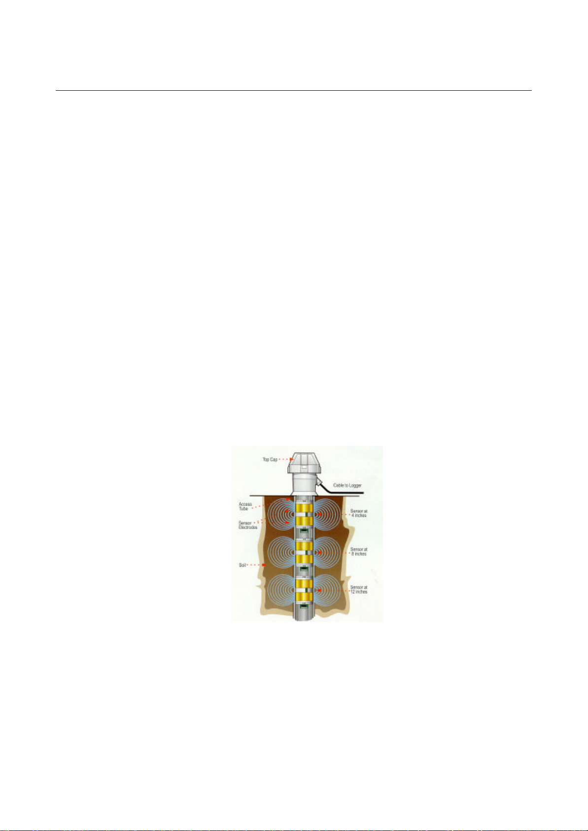
Access Tubes

During installation, the probe is lowered into a specially extruded plastic tube inserted into the soil at the desired measuring location. Readings of soil water content and soil salinity are taken through the plastic access tube without any direct contact between the sensor and soil. The top and bottom of the access tube is sealed to prevent the entry of water and moisture. The top cap of the access tube allows cable entry from the probe to a suitable data logger through a water-tight grommet.

The TriSCAN EasyAG probes are lowered into the smaller diameter EasyAG access tube body.

Figure 1. Cut-away view of the TriSCAN probe

Probe Interface and Data Acquisition Systems

The TriSCAN can be fitted with two probe interfaces: SDI-12 and RS232/RS485 Modbus. This means that data loggers supporting the SDI-12 or RS232/RS485 Modbus protocol can be used to connect and log soil water and salinity data.

Page 13

TriSCAN Manual Version 1.2a

TriSCAN Applications

A Fertilizer Management Tool and Soil Salinity Early Warning System

Sentek has developed TriSCAN to provide a tool for monitoring, understanding and managing irrigation water and nutrients, so that they are maintained within the active crop root zone, where they are taken up to the benefit of the plant and irrigator. These are key challenges of irrigation management today to generate long term, sustainable irrigation practices.

TriSCAN is designed to be a pro -active day to day on-farm management tool for irrigation and fertilizer application, to visualize and prevent leakage of water and nutrients from agricultural production systems. TriSCAN is also designed to report rising salinity levels below or in the active plant root zone and so to provide an early warning system of salinity impact on the plant.

Note: If TriSCA N is to be used as an early warning system to detect damaging salinity concentrations,

salinity benchmarking (a soil salinity check) should be undertaken – refer the section on Salinity

Benchmarking.

Near-continuous data of soil water and soil salinity taken at multiple levels in the soil profile provides a picture of:

• where the roots are taking up water

• the depth of the active root zone

• the day -to-day concentration changes of salts and applied fertilizers

This is a new, dynamic approach linking soil water and salinity to management of irrigation and fertilizer applications; an approach that practically and commercially cannot be achieved using soil sampling alone.

The TriSCAN technology is designed to reduce the soil sampling frequency and it is designed as a complementary technology that will allow soil sampling to be undertaken at strategic points in time.

Determination of EC or ECe in soil samples will verify the magnitude of salinity chang e detected by the TriSCAN sensors. This process is called “salinity benchmarking”, that sets the upper and lower limits of the soil salinity range encountered in the field during the crop season.

Benefits of TriSCAN Applications

The use of the TriSCAN technology can potentially lead to several benefits depending on the user, application and site conditions. These benefits include:

• Optimizing fertilizer uptake by the crop

• Fertilizer savings

• Optimizing crop quality and yield

• Improving economic return

• Minimizing fertilizer leaching into groundwater

• Preventing soil acidification from nitrate leaching

• Providing water savings

• Providing energy (pumping cost) savings

• Improving soil & water conservation

• Reducing leakage from field systems

• Improving irrigation and salinity management

• Reducing costs to the environment and grower

• Conforming to regulatory compliance

• Improving and contributing to the scientific understanding of the water and solute (salt/ fertilizer)

movement in soils

Page 14

TriSCAN Manual Version 1.2a

How does the TriSCAN sensor work?

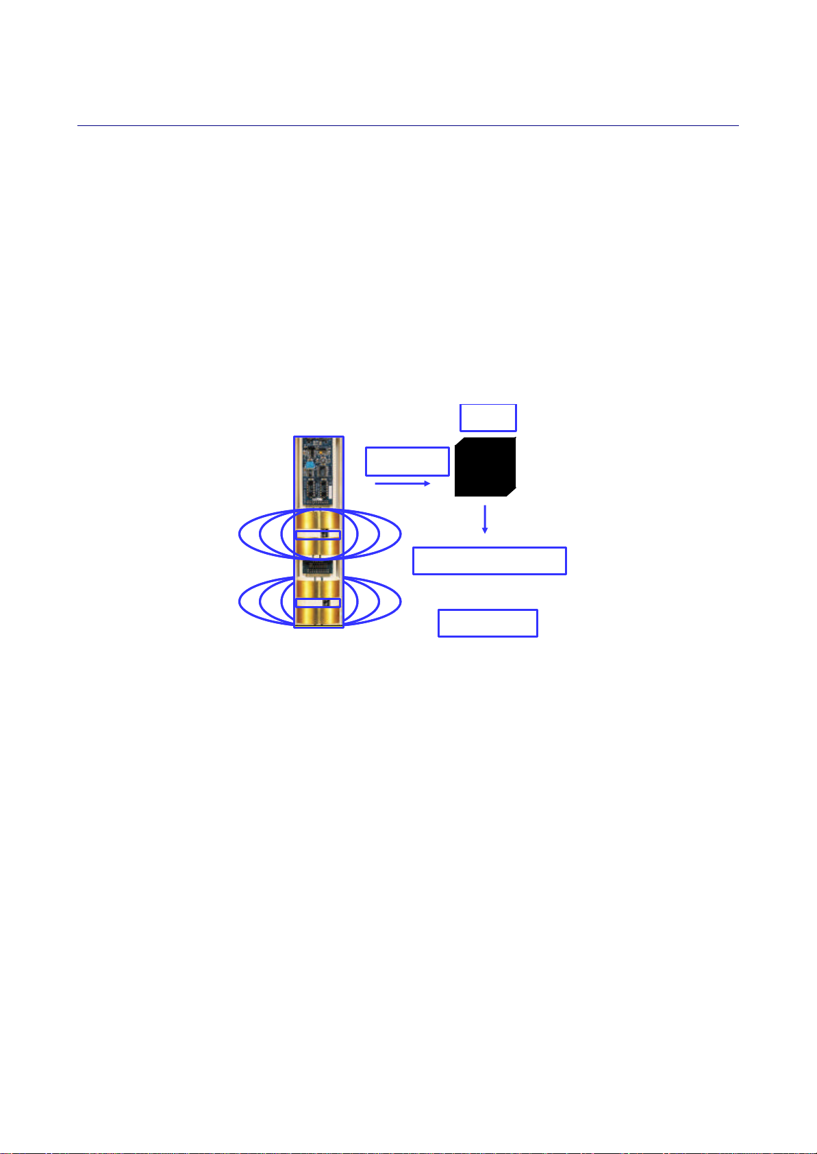
Sensor output and measurement units

The TriSCAN sensor provides two outputs. The first output is a signal of dimensionless frequency (raw count), that is converted via a normalization

equation and then a default or user-defined calibration equation into volumetric soil water content. The measurement unit is thus volumetric water content (Vol %) or millimetres of water per 100 mm of soil depth.

The second output is also a dimensionless frequency (raw count) that, in conjunction with the first output signal, is proportional to changes in soil water content and salinity. A proprietary data model processes the changes of both output signals simultaneously to reflect the changes in soil salinity. The output of the data model is a nominal Volumetric Ion Content (VIC). Measurement units of VIC can be quantitatively related (benchmarked ) to the soil EC through site-specific soil sampling and analysis.

Figure 2. Sensor output

Both outputs can be presented as dynamic trend changes over a chosen time scale.

Raw Data

Soil Water Content

Model

Soil Salinity

Measurement Range and Soil Suitability

The effective measurement range of TriSCAN is between 0 and 17 dSm-1 in sand, loamy sand and sandy loam textures (Australian Soil and Land Survey Field Handbook). Use of TriSCAN at salinity levels and soil textures outside this range is currently unsupported by Sentek.

Resolution and Accuracy

The resolution and accuracy of the sensor can be considered in terms of the two different outputs.

Volumetric Water Content:

The sensor has a resolution of 0.1 mm of soil moisture. Consecutive readings in equilibrated soil have a coefficient of variation of 0.1% .

The accuracy of the system is dependent upon the similarity of the soil site to that of the original default soil type used by Sentek. Calibration coefficients based on this default soil type are used in normal operation. If site-specific (quantitative) values are required, then a calibration procedure is required to be performed (refer to “Calibration of Sentek Probes” Manual). A high level of accuracy can be attained with careful calibration.

Page 15

TriSCAN Manual Version 1.2a

Salinity:

There are two levels at which resolution and accuracy may be considered with regard to the TriSCAN® sensor:

• Resolution and accuracy of the electronic sensor

• Resolution and accurac y of the benchmarking (correlation of VIC to EC) procedure

The resolution of the electronic sensor, i.e. the smallest measurable increment , has been determined to be as low as 1 microSiemen/cm (0.001 mS/cm) in dry soil conditions, and as high as 14 micoSiemen/cm (0.014 mS/cm) in saturated soil conditions.

The accuracy of the benchmarking of the VIC values to soil EC is dependent upon the degree of alignment possible as limited experimentally. This is affected by many things, including the ability of the operator to measure the physical EC, soil sampling technique and sample timing. In Sentek’s own field testing, strong relationships (r2=0.9) have been achieved (refer Figure 8, Benchmarking section).

At Sentek’s laboratories, the accuracy of the sensor to predict the EC has been determined at ±8.06% (range: 6.0 – 10.1%). This figure was determined through analysis of the inherent variability of discrete salinity measurements as taken over a range of water contents from 4% (dry sand) to 20% (saturated) and a salinity range from 0 to 4.9 mS/cm.

Temperature Effects

The precise temperature effects on TriSCAN data output are currently unknown. It is however, known that there is a minor positive relationship between VIC and soil temperature. The TriSCAN model currently does not include temperature correction.

In the field the graph pattern produced is easily discernable as a small temperature effect distinct from salinity changes.

Page 16

TriSCAN Manual Version 1.2a

Getting TriSCAN ready for logging

Probe Assembly and Sensor Addressing

Assembling the Probe

The TriSCAN probe consists of the following components:

• Handle set with screws

• Interface board

• TriSCAN sensors

• Probe Rod

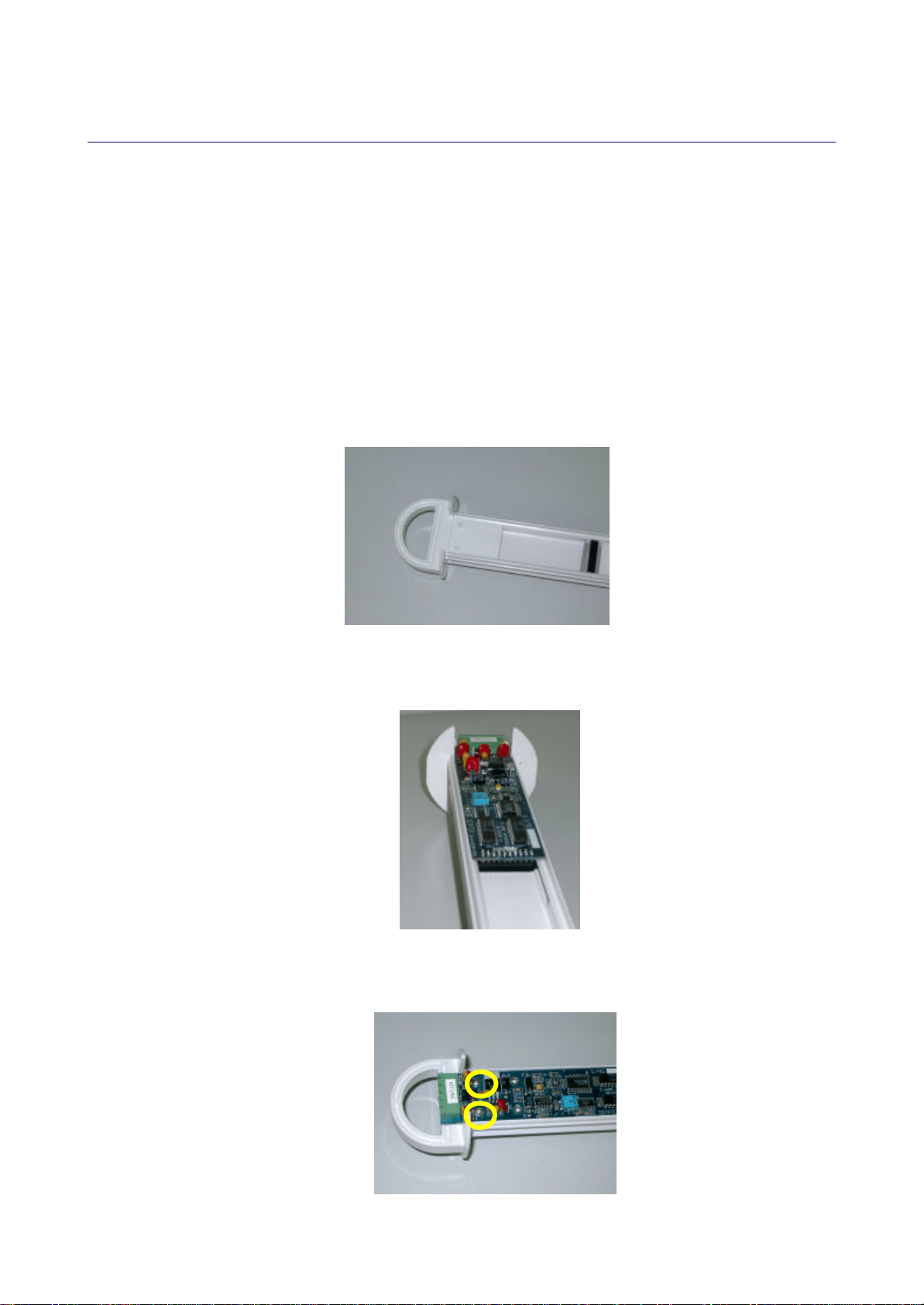
Assemble the probe following these steps:

1. Insert the probe handle into the top of the probe rod, with the lugs on the handle facing the connector side of the probe rod.

2. Attach the interface board to the probe rod. Fit the interface board between the lugs on the handle and the probe rod guides, with the green phoenix connector facing the top of the probe. Plug the interface into the first available connection on the probe rod.

3. Gently move the interface board along the probe rod so that the holes at the top of the board align with the holes in the probe rod handle behind. Insert the two small scre ws into these holes, being careful not to over-tighten.

Page 17

TriSCAN Manual Version 1.2a

4. Insert the large screws into the holes in the side of the handle and tighten to hold them in place. Be careful not to over tighten the screws, as this may damage the interface board.

5. Locate the desired sensor positions on the probe rod, keeping in mind that each probe connection is spaced 100 mm apart.

6. Position the sensor at the bottom of the probe rod with the ribbon cable facing towards the bottom of the probe and the connec tor facing the side of the probe rod that holds the connector plugs.

7. Depress the lever on the bottom side of the sensor, and slide the sensor along the probe rod into position.

8. Align the lug on the back of the sensor with the notch in the probe rod, and click into position by pushing the lever outwards with a finger or screwdriver inserted behind the lever.

Page 18

TriSCAN Manual Version 1.2a

9. Firmly plug the sensor into the connector on the probe rod, ensuring that all the pins are correctly aligned.

10. Repeat for the other sensors.

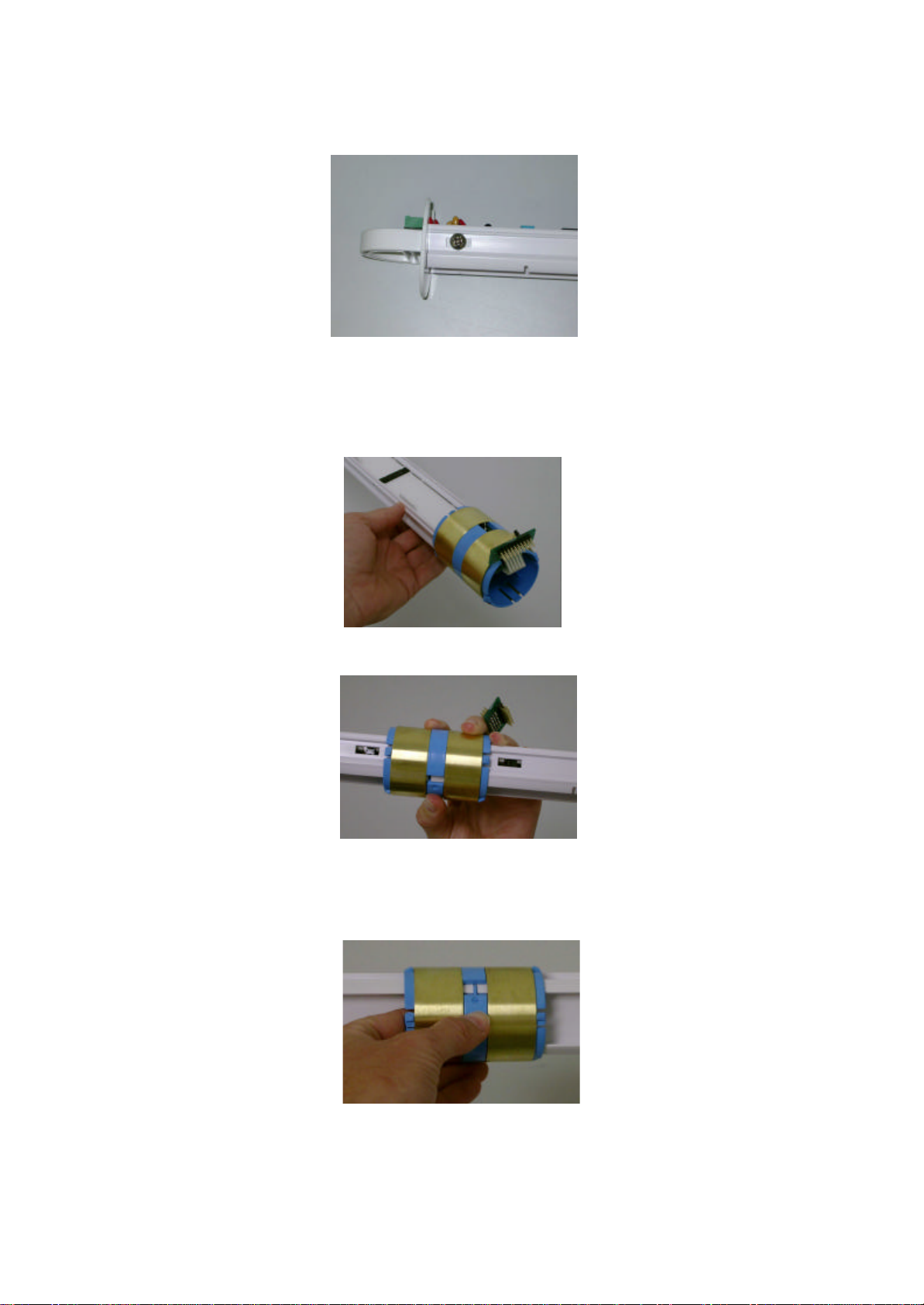
Addressing the Sensors

After positioning and securing each sensor in its proper location, every sensor on a probe needs to be assigned a unique address. The sensor address is set by changing the position of the address link on the ribbon cable board of the sensor. This address is a means of differentiating between each sensor on the probe, and can be assigned a numerical value between 1 and 16. The sensor address is not necessarily related to the sensor position on the probe rod.

Figure 3 below shows the address link in position 5 on the sensor.

Figure 3. Example of sensor address 5

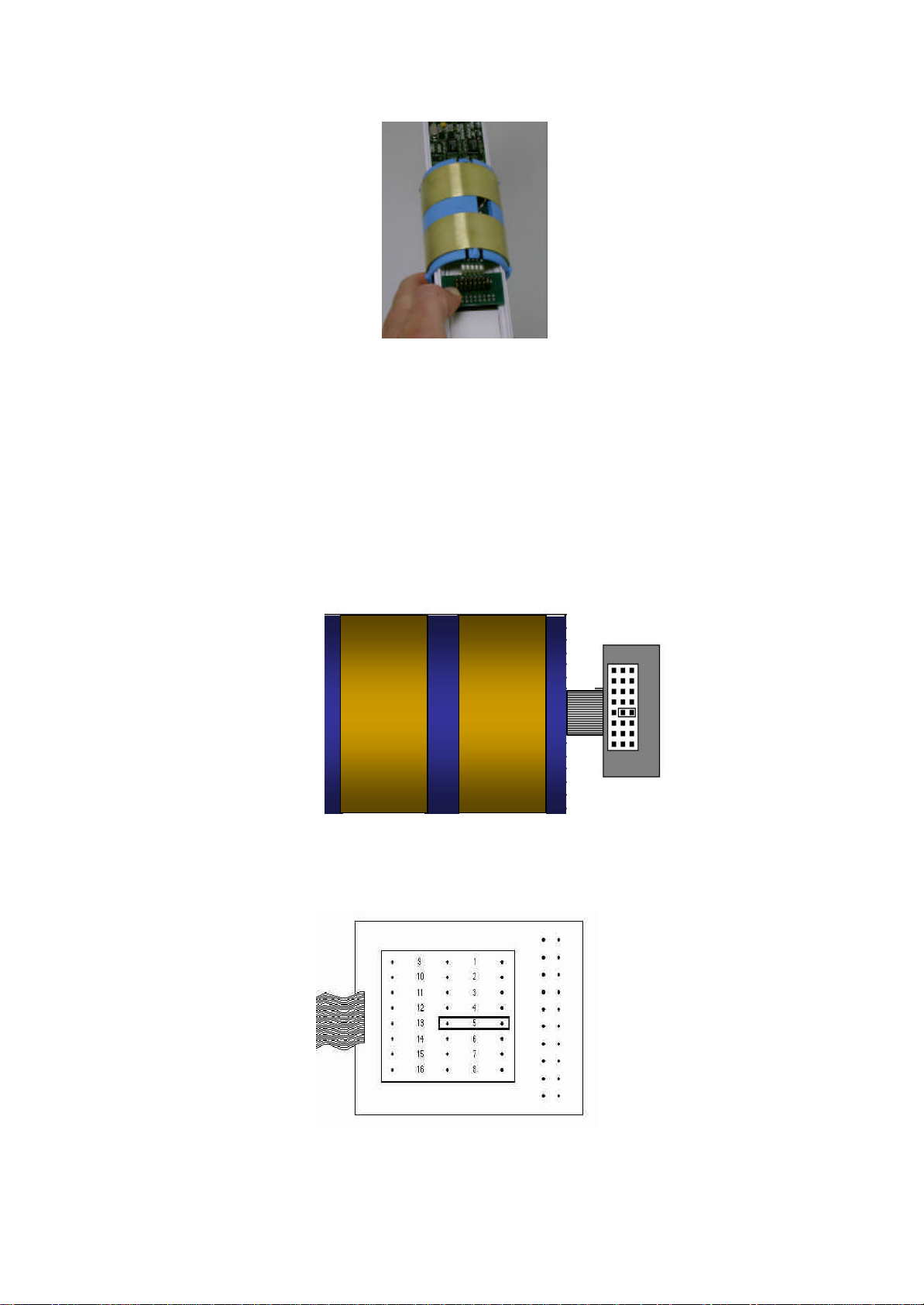
Figure 4 below outlines the sensor address link positions for all the different possible addresses.

Figure 4. Sensor addressing positions

Page 19

TriSCAN Manual Version 1.2a

For each probe, assign the top sensor with the lowest address (e.g. address 1) and then address each sensor below it with a sequentially higher address, such as 2, 3, 4 and so on.

Probe Configuration and Normalization

The probe is now ready to normalize. The following paragraphs outline the procedure for normalizing the probe using the IP Configuration Utility Software Version 1.4.1 or later. For more details on the IP Configuration Utility Software, refer to the IP Configuration Utility User Guide.

Step 1 – Powering the probe

Connect a 12 volt power supply to the probe. Refer to the relevant SDI-12 or RS232/ RS485-Modbus Manual for the correct wiring procedure. Power can either be supplied from the logger power source or directly to the probe.

Warning:

Incorrect wiring may lead to damage to the probe, or blow the fuse on the probe interface. Any damage

due to incorrect wiring will void the warranty. Therefore it is recommended that the wiring procedure be

checked prior to connecting the power to avoid such damage.

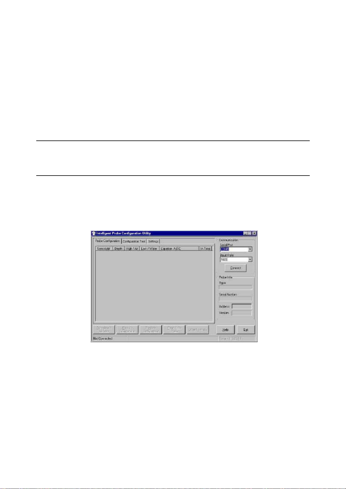
Step 2 – Connecting to IP Configuration Software Utility

1. Connect the IP Configuration Utility Cable to the probe interface and to the serial port on the computer.

2. Open the IP Configuration Utility Software.

3. Select which serial port the probe is connected to from the Serial Port drop down list. Also select the baud rate to use from the Baud Rate drop down list. If you are unsure of the baud rate you can select “Auto” for the baud rate which will use auto detection of the baud rate when connecting.

4. Click the Connect button to connect to the probe. If connection is successful then the status bar will now display “Connected” and the Connect button will have changed to Disconnect. If “Auto” was specified as the baud rate then the correct baud rate will now be displayed in the Baud Rate drop down list. On successful connection, the probe’s information (name, serial number, address and firmware version number) will be displayed, and the probe will be queried for its configuration settings.

Page 20

TriSCAN Manual Version 1.2a

Step 3 – Getting the configuration from the probe

To detect the probe configuration, click on the Auto-detect Sensors button. This will automatically detect all the sensors on the probe. After the sensors are detected the configuration information will be displayed in the list.

Step 4 – Changing the sensor depths

1. Click on the sensor depth when it is selected and it will go into edit mode as show n above.

2. Type the new depth or use the up/down arrows to increase or decrease the depth value 10 units at a time. The minimum allowable depth is 5.

3. To accept the new depth, click outside the cell or press Enter. The new depth will not be set in the probe’s configuration until you use the Write to Probe button. If you want to discard the changes, press Escape and the depth will change back to the old value.

Note:

The depth number is not associated with any units and is just a stored value for informative purposes.

Therefore the value may mean "inch", "cm", etc.

Step 5 – Normaliz ing the sensor air and water counts

The effective range of each sensor needs to be set between a high and low value. To achieve this each sensor is normalized under identical conditions.

To normalize the air counts:

1. With the probe inside an access tube and held in the air, click on the buttons in the “High / Air” column one at a time to start direct sensor reading. Ensure that the probe is held well away from any objects when obtaining the air counts.

2. Wait for a few seconds at each sensor while the reading stabilizes before clicking on the next one.

To normalize the water counts:

1. Insert the probe into the tube in the normalization container filled with reverse osmosis (RO) water (EC less than 300µScm-1), so that the sensor that you wish to take the water counts from is in the centre of the tube.

Note:

The water in the normalisation container must be RO water for TriSCAN sensors, as other water supplies

may contain ions that affect the reading of the sensor.

2. Click the button in the “Low / Water” column that refers to that sensor to start direct sensor reading mode. Wait until the reading stabilizes and the value displayed is updated. To accept the new water count value click the button again to stop direct sensor reading.

Page 21

TriSCAN Manual Version 1.2a

3. Repeat this process for each sensor on the probe.

The expected air and water counts are dependent on the sensor type and sampling mode. Normalization values outside the expected range may indicate errors in the normalization steps or problems with the hardware.

Table 2. Expected air and water counts for different sensors

Sensor Type Sampling Mode Air Range Water Range

EnviroSCAN sensor (white) Moisture 36000±3000 23000±3000 TriSCAN sensor (blue) Moisture 33000±2000 22800±2000 Salinity 20500±2000 13500±2000 EasyAG sensor (white) Moisture 44000±2000 31000±2000 Moisture (sensor at bottom) 50000±2000 32000±2000 EasyAG with TriSCAN sensor (blue) Moisture 33000±2000 25000±2000 Salinity 20500±2000 15000±2000

Step 6 – Changing the Calibration Coefficients

To change the calibration coefficients of the sensors:

1. Click on the sensor coefficients cell when it is selected and it will go into edit mode as shown above.

2. Type the new coefficients separated by semicolons. To accept the new coefficients click outside the cell or press Enter. If you want to discard the changes while in edit mode then press Escape. The new coefficients will not be set in the probe’s configuration until you use the Write to Probe button.

The default calibration equation coefficients provided for different sensor types are listed in Table 3.

Table 3. Default Calibration Coefficients

Sensor Type A B C

Moisture sensors 0.1957 0.404 0.02852 TriSCAN sensors

1.0 1.0 0

Step 7 – Addressing the Probe

Where there are multiple probes connected to a logger in a multi-drop situation, it is necessary to assign each probe a unique address to avoid a clash in communication.

Page 22

TriSCAN Manual Version 1.2a

To change the probe address, type the new address in the Address tab on the Probe Configuration page. The address of the probe should be in the range 1-65534 for most types of probes. Probes supporting specific protocols such as SDI-12 and Modbus accept only addresses in their specific formats (i.e. ASCII '0''9', 'a' -'z', 'A'-'Z' for SDI-12 probes, 1 to 247 for Modbus probes).

Step 8 - Writing the Configuration to the Probe

Writing the configuration to the probe will send the currently displayed sensor configuration (and output port configuration, if applicable) to the probe. The probe’s address will also be set to the one displayed in the Probe Info section. Existing configuration information in the probe will be overwritten. If you do not write the configuration to the probe, the changes to the probe configuration will not be saved onto the probe itself.

To write the configuration to the probe:

1. Click the ‘Write to Probe’ button. You will be prompted to make sure you want to write both the sensor configuration and the probe output port configuration (if applicable for the connected probe) to the probe.

2. Click ‘Yes’ and the configuration information for that page will be written. Settings will be verified when you click the ‘Write to Probe’ button.

Step 9 – Backing up the Configuration File

The Probe Configuration information should be saved as a configuration file. This is useful if the probe interface ever needs to be changed, as the original probe configuration (i.e. depth settings, air and water counts, probe address and calibration coefficients) can then be written to the new interface.

To backup the configuration to a file:

1. Click the Backup Configuration button.

2. Specify the file you would like to save it in and click OK. The sensor configuration (and probe output port configuration, Modbus or Analog if applicable) information displayed should now be stored in the specified file.

Important Information for Configuring TriSCAN probes

The probe configuration page is for displaying and editing the probe configuration.

The colour red represents an item that has been modified, and an asterisk appears on the title tab to indicate some change has occurred on that page, which has not been written to the probe (this will remain until ‘Write to probe’ is performed).

Page 23

TriSCAN Manual Version 1.2a

Some important information on the configuration of the TriSCAN sensors is summarized in Table 4.

Table 4. Configuration Information for TriSCAN sensors

Sensor Address

Displays the sensor address for each sensor. Note 1: Moisture sensor addresses start at 1. The sensor address is controlled by the

address jumper plug on the physical probe sensor assembly (refer to section of Probe Assembly and Sensor Addressing). Non-existent sensors will not be assigned a sensor address e.g. On an EasyAG -50 probe sensor addresses are detected as 1, 2, 3, 5 (no sensor 4).

Note 2: Salinity sensor addresses start at 65 in firmware that supports salinity. If salinity sensor addresses start at 129 then the firmware loaded in the probe does not support salinity and sensors readings will be indeterminate.

Note 3: Temperature sensor addresses start at 129 in firmware that supports salinity sensors (earlier firmware versions have a temperature sensor at address 66). At present only one temperature sensor exists and it only samples the temperature on the interface device circuit board. This sensor is only accessible using this IPConfig program and cannot be accessed through the output port.

Note 4: Salinity sensors (if present) always correspond to a moisture sensor address i.e. salinity sensor 65 is associated with moisture sensor 1, 80 with 16 etc.

Note 5: The sensors are sorted by type (moisture, salinity, temperature) then depth, then sensor address. This sort order cannot be changed.

Depth Depth of each sensor.

When a new sensor is detected a depth of value '0' (zero) is assigned to it. This indicates that the sensor has not been configured yet. Clicking a depth when the row is selected allows changing the depth. Pressing Enter or clicking outside the cell confirms the changes. Pressing Escape discards any changes. The depth figure should reflect the actual (physical) depth of each sensor.

Note: The depth number is not associated with any units and is just a stored value for informative purposes. Therefore the value may mean "inch", "cm", etc.

The following notes only apply to firmware that supports salinity sensors . You cannot directly set the depth of salinity sensors. The depth is taken from the

corresponding moisture sensor depth. Warning:

The depth of a salinity sensor remains zero until the following steps are performed.

1. The corresponding moisture sensor depth is set.

2. The salinity sensor is normalized (air and water counts set).

3. Write to Probe has been performed.

4. The salinity depths (using IPConfig version 1. 4.1) are not updated after the above steps, until “Read from Probe ” (or Disconnect/Connect) has been done.

High / Air Displays the high counts of the sensor. This field contains buttons for taking new air

counts from moisture and salinity sensors. Clicking on these buttons will start or stop direct sensor reading for that sensor.

Low / Water Displays the low counts of the sensors. This field contains buttons for taking new water

counts from moisture and salinity sensors. Clicking on these buttons will start or stop direct sensor reading for that sensor.

Equation A;B;C

Displays the calibration equation coefficients for the sensors. The A, B and C components of the equation must be separated by semicolons. Clicking on the calibration equation when the row is selected will enable editing of these coefficients. Pressing Enter or clicking outside the cell confirms the changes. Pressing Escape discards any changes.

Page 24

TriSCAN Manual Version 1.2a

In Total Sentek Smart Probes support a feature, by which the probe can provide a sum of values

of the selected sensors. This is useful when an overall amount of water in the soil profile is to be found. A tick specifies that the sensor is used in the “In Total Moisture Calculations”. Double click in this column to change which sensors are used. A red cross or a blank cell specifies that the sensor is not used in the “In Total Moisture Calculations”.

Note: Early probe versions do not allow de-selection of all sensors from the ‘In Total’ reading.

Page 25

TriSCAN Manual Version 1.2a

Site Selection

The key to effective soil water and soil volumetric ion content (VIC) monitoring is to select sites which truly represent irrigation management areas. The same basic site selection principles apply to the full range of Sentek soil moisture and salinity monitoring devices.

In addition, when monitoring soil solution VIC, consideration of VIC variability in relation to the irrigation emitter needs to be taken into account.

Many variables influence the spatial distribution of soil water and VIC across an area of land. These variables and their impact on site selection are discussed in more detail below.

What is site selection?

A site is defined here as: “The location of the access tube within a field or irrigation shift, where soil water and soil volumetric ion content (VIC) readings are taken at different depth levels within the soil profile.”

Note:

If readings are to be used as a basis for scheduling irrigation; managin g fertilizer applications or

monitoring salinity, it is imperative that monitoring sites are representative of these areas.

Soil moisture data can provide information about the:

• Quality and depth of irrigations

• Levels of soil moisture retention

• Depth of the crop root zone

• Impact of weather and rainfall events on an area

Soil VIC data can provide information about the:

• Movement of ions within the profile

• Uptake of ions by the plant or loss to the atmosphere

• Leaching of salts below the root zone

• Excessive build-up of salts within the root zone to detrimental levels

Warning:

Do not position TriSCAN sensors at random on your property. Poor site selection will result in

unrepresentative soil moisture and salinity data.

Site selection is carried out in two stages:

• Macro zone selection

• Micro zone selection

Relationship between macro and micro zones in the field

Traditional practice within the field and across the whole farm is for irrigation and fertilizer to be applied on a hypothetical “farm average” – similar to traditional broad acre management practices.

Uniform application of irrigation and fertilizer across areas with highly variable soils, nutrient levels and different levels of crop water use causes significant differences in yield and quality. This creates commercial losses and environmental harm through increasing problems with rising water tables and increasing salinity.

Page 26

TriSCAN Manual Version 1.2a

If different soil types are ignored in terms of their different irrigation scheduling requirements and nutrient management, crop setbacks or failures may occur. This effect is displayed in the aerial photograph of a citrus orchard (Photo 1).

Photo 1. Variable growth due to uniform management across variable soil types

Macro zone selection defines the number of zones on a property where the amount and timing of irrigation and fertilizer applications can be specifically tailored to match soil and crop variability. A macro zone thus comprises areas with similar crop water and nutrient requirements and salinity characteristics.

Crop water use is governed by many factors such as soil properties; water quality; weather patterns and type of irrigation system. These factors need to be considered when defining the macro zones on your property.

Micro zone selection determines the position of access tubes in relation to the crop and irrigation system. Micro zone selection considers the:

• areas of root zone and canopy spread

• water distribution uniformity (sprinkler pattern)

• moisture patterns of drip irrigation

• surface, topographic and soil anomalies

The consideration of these factors will help you find the best representative position or site for access tube placement within the macro and micro zones.

Macro and micro zone selection is described in greater detail in the following pages. If you require further information, consult your Sentek reseller and/or undertake further reading.

Important factors for macro site selection

Many factors can have an impact on the way the water is stored in the soil and on the way crops use that water. They affect transpiration and evaporation rates and have a direct impact on irrigation scheduling. In macro zone selection, it is important to consider the way the following factors influence water use in a particular area or zone:

• Climate

• Soils

• Crop

• Cultural management

• Irrigation system

• Water quality

Page 27

TriSCAN Manual Version 1.2a

Climate

The most commonly recognized factor in influencing the amount of crop transpiration is the weather.

Temperature

Crops need to draw up water to compensate for water use through transpiration (water loss through the leaves) and evaporation (water loss from the surface of soil and leaves). The demand increases with increasing temperature up to a maximum threshold for each crop (when the stomata close and photosynthesis stops).

Humidity

Atmospheric demand for transpiration and evaporation is relative to the humidity (amount of water vapor in the air). The higher the humidity level, the lower the demand.

Wind speed

Crop transpiration and evaporation increase with increasing wind speed, creating an increased water demand. At higher wind speeds, transpiration eventually decreases due to stomata closure, but evaporation increases.

Solar radiation

On sunny days, crops can synthesize more basic sugars and complex plant food compounds, through combining atmospheric carbon dioxide and soil-derived water, than on cloudy days. Although crops vary in their sensitivity of photosynthetic response, they all require access to greater amounts of soil water.

Rainfall

Rainfall is generally associated with higher humidity levels and lower solar radiation and temperatures. It follows logically, than days on which rainfall occurs, are associated with lower water demand and use than dry, sunnier days.

Notwithstanding the care taken to delineate macro zones, some variability in soil moisture levels is inevitable. For example: on large properties rain events may cover only a portion of the agricultural area, replenishing some soil reservoirs and leaving others dry.

The aspect or orientation of sloping fields can subject the crop to more or less solar radiation, wind exposure or water run -off – all affecting crop water use.

Soils

An understanding of how soil type influences plant -soil-water dynamics, and hence irrigation scheduling is important. Intrinsic soil properties are texture, structure, depth, soil chemistry, organic matter content, rocks and stones and clay type. Influencing factors include compaction, salinity, water -table development, drainage rate dynamics and topography.

Soil texture

Water storage in the soil profile depends on the soil texture. At the one end of the spectrum, sandier soils with a low porosity (total volume of pore space) and weak adhesion forces (strength with which water and nutrients are held), fill up and drain quickly. The nutrient holding capacity is also low and hence these soils, in general, require smaller and more frequent irrigations and fertilizer/fertigation applications. In contrast, the heavier clay soils have a high porosity and strong adhesion properties. Consequently, they replenish and drain slowly and to a higher total water content than lighter (sandier) soils. Nutrient holding capacity is also high. An infinite range of textures exist between the two extremes. Textures often change within a profile, with the layering of different textural bands playing a large part in determining the water holding capacity of a soil.

Soil structure

Water infiltration rates, and air and water permeability within the soil profile are closely related to the size and distribution of soil pores (porosity). Porosity, in turn, is dependent upon the arrangement and aggregation (binding) of sand, silt and clay particles (soil structure). Soil structure is as important as soil

Page 28

TriSCAN Manual Version 1.2a

texture in governing how much water and air move in soil and therefore their availability to crops. Roots penetrate more easily and rapidly in soils that have stable aggregates, than in similar soil types that have no or highly developed structures. The effectiveness of soil moisture, air and nutrient utilization, is related to the efficiency of root colonization of the entire soil profile.

Soil depth

The effective depth of soil affects the extent of root penetration. The deeper the soil, the greater the volume of soil that is available for gas eous exchange and water and nutrient uptake. Drainage is also affected by effective depth.

Soil compaction

Soil compaction from farm machinery can change pore size and distribution resulting from the natural arrangement of the sand, silt and clay particles. This can cause reductions in water infiltration rates, and air and water permeability within the soil profile. The resultant impact upon the effectiveness of root penetration, air exchange and nutrient and water uptake, affects plant growth efficiency and hence water and nutrient uptake.

Salinity

Salinity lowers osmotic potential, reducing the efficiency with which nutrients and water are taken up by the plant. The dominance of the contributing ions can result in a nutrient imbalance causing deficiencies of essential macro and micro nutrients. The reduced plant health and vigour affect crop water use.

Water tables & drainage rate

Poor drainage can lead to the development of water tables and/or cause a temporarily saturated soil profile. The presence of impermeable soil layers can cause the formation of perched water tables, which saturate parts of the root zone. Efficient gaseous exchange becomes impossible, and plant health and water use is reduced.

Organic Matter

The presence of organic matter and humus increases the cation exchange capacity (CEC), water -holding capacity and structural stability of soils. This influence is predominantly in the top soil, although lamellae (thin organic matter layers further down the profile) can be important properties.

Type of clay

Clays are highly variable in their water -holding capacity, CEC (ability to hold and release nutrients) and stability (shrink -swell potential). At the one end of the spectrum, the so-called smectite-type clays have high CEC’s, water-holding capacities and low stability. Highly weathered (kaolinite or oxide) clays, at the other extreme, are stable with relatively lower CEC’s and water -holding capacities. Most soils have a mixture of clay types depending on parent material and climate. At present TriSCAN is only recommended for predominantly sandy soils.

Soil chemistry

Acid, alkaline, sodic (soils characterized by a dominance of sodium ions) or nutrient deficient conditions impact on expected soil chemical properties. For example:

• pH conditions change CEC; the availability of nutrients (by changing their form) and the solubility of ions.

• High levels of sodium can lead to structural collapse.

Rocks and stones

Stones and rocks within a soil profile occupy part of the soil volume and hence reduce the soil water storage capacity. Very stony soils have a substantially lower water holding capacity than soils of the same texture that are free of stones.

Page 29

TriSCAN Manual Version 1.2a

Topography

Topography relates to the configuration of the land surface and is described in terms of differences in aspect, elevation and slope. This impacts on plant-soil-water dynamics via influencing climatic conditions including:

• Rain shadows and sunshine hours

• Rainfall and temperature patterns up slopes

• Elluviation (washing-out) of clays from higher elevations and illuviation (washing-in and

accumulation) of clays at lower elevations

• Relatively poorer drainage at lower elevations

Crop

Crop differences have an impact on crop water use and irrigation scheduling requirements. While all require management between full point and refill point at most times, the depth of root extraction varies, as do specialized requirements e.g. the deliberate stressing of horticultural crops during flowering.

Most plant tissues contain about 90% water and the rate of uptake of water from the soil solution by plant roots is largely controlled by the rate of water loss through transpiration. Plant characteristics such as crop type, size, age, vigour, variety, rootstock, development stage, leaf area, nutritional status, disease status, crop load and harvest all affect crop water use. Specialized advice should be sought in this regard. A rough guide to water use can be obtained from crop coefficients, which are widely available in the literature for different stages of growth for most crops (Table 5). These express evapotranspiration as a ratio of reference evaporation (in this case Penman-Monteith).

Table 5. Examples of crop coefficients (FAO)

Crop Kc (initial) Kc (mid) Kc (end) Green beans 0.5 1.052 0.9

Artichokes 0.5 1 0.95 Cereals 0.3 1.15 0.4 Sugar cane 0.4 1.25 0.75 Alfalfa 0.4 0.95 0.9

Cultural Management

The impacts of cultural management (agronomic/horticultural practices) also need to be understood for proper irrigation scheduling.

Soil preparation

Cultivation increases evaporation from the topsoil, reducing soil water available to the plant. It may also reduce water run -off and improve the infiltration of rain and irrigation water, improving plant water availability. The dynamics of nutrient availability are also affected. An example is the dependence of mineralization rates, of particularly nitrogen, upon aeration.

Cover crop and mulch

Cover crops provide more competition for water, but reduce evaporation and facilitate infiltration of rain and irrigation water, reducing run-off.

Mulch can improve the infiltration rate of the soil, reduce water run-off, encourage root growth near the soil surface and increase the soil water holding capacity over time, through the accumulation of soil organic matter, and reduc tion of soil temperature.

Oil spraying

Oily substances on leaves reduce water use by temporarily closing stomata. An example of this is mite control in citrus.

Page 30

TriSCAN Manual Version 1.2a

Fertilizer management

In order to ensure that no nutrients are deficient, fertilizer applications are normally based on soil and/or leaf sample analyses. The degree of precision varies from a rough averaging approach, to precision farming where sample points are matched to requirements using satellite tracking technology. He althy crops require more water and have different nutrient dynamics to crops that have been stunted or diseased through inefficient fertilizer management.

Pest/disease management

Good pest/disease management keeps the crop protected and in good health, sustaining its potential growth and transpiration rates. Infestations can result in lower than normal water and nutrient uptake.

Irrigation System

Variations in irrigation system pressure, flow and water distribution uniformity cause variations in irrigation application. This affects root zone wetting patterns and therefore crop water use.

The preceding crop water use factors should be taken into account when matching your irrigations to areas of similar crop water use. These areas are then represented by soil water monitoring sites and the data collected at these sites is used for irrigation scheduling purposes.

Water Quality

The source and constituents of irrigation water, impact on osmotic potential (and hence plant water uptake). Measured volumetric ion content (VIC), will increase with increasing irrigation water electrical conductivity (EC). Water quality can vary both within and between seasons and between water sources.

A general view of macro scale zone selection

Macro zone selection is used to ide ntify the total number of required zones and their locations on your farm. A macro zone comprises areas of similar crop water use and fertilizer requirements.The aim of good site selection is to select a monitoring site that reflects representative changes in soil water content, fertilizer mineralization and crop water / fertilizer use trends.

The representative data gained from monitoring sites is used to schedule irrigations over a larger defined area. This area (or macro zone) may be an entire field, or a sub -section of a field, where irrigation is applied during a watering shift or fertilizer application.

As an irrigator, you want to replenish the soil water used by plants for growth and transpiration, whilst maintaining nutrients at a level sufficient to ensure growth, but not too high so as to cause leaching losses. It is important to understand the many factors affecting crop water use or transpiration and how these factors may vary on your property.

A primary goal of good irrigation management is to match irrigations to areas with similar crop water use, within the limits of your irrigation system flexibility. This consideration will ultimately determine how many monitoring sites you will need and where you should locate them. The diagrams on the following pages show how ‘factors that affect crop water use’ can be used to determine macro zones.

Firstly the topography must be considered,

Page 31

TriSCAN Manual Version 1.2a

Then the soils,

Then the type of irrigation and system layout,

And finally, the crop types.

Overlaying all this information makes it possible to identify, within a property, areas (zones) that have significantly different requirements.

In the example used, the property has been divided into four macro zones. Each macro zone requires a monitoring site. Potential sites are shown by the dots, but final positioning can be determined by the information in the micro scale zone section.

Page 32

TriSCAN Manual Version 1.2a

Micro scale zone selection

During macro zone selection you identified the irrigation management units on your property. Micro scale zone selection target s the actual site of the access tube in relation to crop and irrigation delivery point.

Note:

Micro zone selection is equally as important as macro zone selection and has a direct effect on the

representative value of the data.

In soil-based monitoring, the measurements are taken from a small part of the root zone. Sentek sensors record the dynamics of moisture in the part of the soil profile where the access tube has been installed. If you miss the root system or install the access tube in abnormally dry or wet irrigation spots, the data will not be representative of the irrigation management unit.

Micro zone selection guidelines

The following is a set of guidelines for selecting access tube installation sites within irrigation management units. Two major factors need to be taken into account; irrigation and plant health.

Irrigation system

It is important to check that your irrigation system is performing as per design specifications prior to installation and at least annually thereafter. Variations in sprinkler pressure and flow, pump performance, distribution uniformity and wind can result in uneven patterns of watering. This can lead to; the development of water tables, dry spots and salinity problems.

Conducting a Distribution Uniformity (DU) test

Prior to installation, it is also necessary to check the distribution uniformity (DU) of the system. This can be done with a simple can test. The method involves arranging cans in a grid pattern, in a representative area within the macro zone. In the example illustrated in Figure 5, cans in the blue shaded area received above average water; those in the red shading below average; while those in the green shading, received an average amount.

Figure 5. Example Water DU test results

A DU of salinity at the proposed probe site can act as a valuable check to ensure that an especially saline or non-saline site has been chosen. Samples should be collected in a grid, at the same depths as the probe sensors. A simple 1:5 EC test for each sample will provide an EC DU. As before excessively high or low unrepresentative areas should be avoided. Areas such as fertilizer preparation or turn -around zones should be avoided.

Figure 6 below illustrates the degree of salinity uniformity found in a potato field. It can be seen that, although the salinity distribution uniformity is high at each depth, it is possible to inappropriately site a probe in a position of high salt by mistake. It also shows the degree of inherent difference in ECe at depth. Greater

Page 33

TriSCAN Manual Version 1.2a

Crop: Potato

soil fertility is indicated at 30 cm depth than at all others. This is indicative of previous cropping history and fertilizer applications.

Figure 6. Example of EC distribution uniformity in a potato field

Irrigation: Centre Pivot Water DU = 79.1% Salinity DU = 86.9% (10cm),

85.4% (30cm), 91.2% (50cm).

Due to the specific nature of each site in terms of irrigation system, cultivation practice and fertilizer application method, it is inappropriate to give prescriptive advice on tube placement. Placement should however be representative and consistent. General guidelines, for commonly used systems, and principles of sample site selection follow:

For sprinkler systems, it is preferable to use two access tubes per site, plac ing one into an area receiving average precipitation and the other into an area of perceived need.

Under centre pivot irrigation,, two or more access tubes should be installed if the distribution uniformity tests show significant variation between booms..

For high pressure rain guns, measure the water application pattern under different wind conditions to ensure that you don’t pick an area of extremely low or high water application.

Installation of access tubes in drip irrigation crops needs consideration of the extent of the ‘wetting onion.’ Use at least two access tubes to monitor soil moisture of drip irrigated crops to measure the lateral spread of water.

In furrow irrigated fields, avoid installing access tubes too close to the head ditch or where tail water from the irrigation may back up the furrows and give unrepresentative readings. Consider also installing an access tube in the middle of the field to measure the depth of irrigation there.

Plant health

Select a site next to an average sized, healthy plant representative of the irrigation management unit (macro zone). Avoid:

• Stunted or sick plants

• Unusually large plants

• Spots where plants are missing

General guidelines for key crops follow:

• In field crop and vegetable production, ensure that the probe is inserted within the actively growing root zone.

• In orchards, use two access tubes to monitor the site. Place one access tube under the canopy of a tree and another outside the canopy. Again take care to select a site that represents dynamic dat a trends (root activity).

Page 34

TriSCAN Manual Version 1.2a

Fertilizer types and application methods

It is essential that notice is taken of the fertilizer application method. The following factors should be taken into account:

• The position of the edge of the wetting pattern, where salts will accumulate

• Points of concentration of fertilizer application, which vary according to application method eg. spot,

within-row, ring or band

• Mineralization rates of fertilizers eg. animal manures, compost and urea.

Other micro zone selection considerat ions

There are several other factors when considering micro zone selection that need to be taken into consideration. These are:

• On sloping ground in drip irrigated situations, install the access tube below the emitter.

• Do not install access tube in outside rows. These locations are usually exposed to wind and dust,.

• Avoid the ‘drip ring’, for example, citrus orchards, where sprinkler irrigation water is channelled by

the canopy to the outside bottom edge of the foliage creating wetter soil conditions at the edge of the canopy.

• Avoid wheel tracks (and wheel track rows) as the soil is more compacted in these areas.

• Inspect the site for any anomalies that could give an unrepresentative picture. These could include

fertilizer spillages , localized salt accumulation or localized drainage non-conformities.

• If water application is not uniform due to uneven land surface, salts will accumulate in high spots with little water penetration and leaching.

• Water accumulating in low-lying areas causes waterlogging and indicat es potential drainage problems.

• With furrow irrigated crops, planted on raised beds, water movement is from the furrow into the bed. Since water moves from the two furrows towards the centre of the bed, any salts present, move with the water and tend to ac cumulate in the upper centre of the bed.

• Salts also accumulate with localized irrigation at the soil surface between emitters, and at the

outside edges of the area wetted by the water applicators. .New plantings can also be affected, if they take place int o these salty areas without prior leaching.

Figure 7: Example of localized salt accumulation in furrow irrigation (after Ayars & Westcott )

Salt accumulation

Page 35

TriSCAN Manual Version 1.2a

Access Tube and Probe Installation

The information provided below is a summary only. Further information is provided in the Access Tube Installation Guide Version 1.0. It is recommended that the probes be installed by a trained Sentek installation specialist.

The aim of the installation is to cause minimum disturba nce to the crop and soil profile. Disturbances to the soil may produce pockets of air or loosely packed soil material. These conditions will cause preferential flow of irrigation water or rain to a greater depth compared with the rest of the field. Access tubes must be installed to fit tightly in the soil along their entire length.

Permanent errors can be introduced into the measurements through poor or hasty installations. Air gaps existing between the sensors (or access tubes) and the soil will bias sens or readings, i.e. the sensor will read high when the air gaps are filled with water and low when they drain. Poor installation is a primary source of inconsistencies between sensors.

The additional time taken in careful installation ensures access to accurate and meaningful data. Sentek has developed precision installation tools to be used for the installation of Sentek access tubes. The precision of the access tubes and tools is designed to complement the high value of the readings taken by the Sentek sensors.

Standard TriSCAN Access Tube Installation Method

The standard manual installation method is recommended for most soil types. In this method the access tube hole is hand augered into the soil, through and slightly ahead of the access tube. This is done using the 47.0 mm Regular Auger. The augered hole is slightly smaller than the access tube. The access tube is fitted with a cutting edge that cuts the last of the soil away, providing a tight fit down the length of the access tube.

This method prevents the formation of air pockets along the length of the access tube and causes minimum disturbance to the surrounding soil profile. This installation method is proven to be reliable.

Installing the Access Tube

To install an access tube, follow these steps:

1. Put on gloves

2. Put on safety goggles

3. Select the 47.0 mm regular auger head

4. Select the required extension rods and screw the auger head and the T-handle to the extension rods. The length of assembled auger must exceed the length of access tube by at least 20 cm.

5. Insert the auger into the access tube while the tube is lying on the ground until the auger head protrudes by 20 cm.

6. Use a marking pen to mark the auger extension rod at the point where it disappears into the top of the access tube.

7. Remove the auger from the tube.

8. Select the yellow cutting edge and push it into the end of the access tube ensuring it fits squarely. Note: If you experience difficulties fitting the cutting edge onto the tube then turn the cutting edge on its side and, with a twisting motion, shave a layer of PVC from the lip of the access tube. Partially fit the cutting edge into the end of the access tube, then gently bounce the access tube and cutting edge on the side of the sledgehammer head until the cutting edge fits squarely.

9. Insert the access tube with fitted cutting edge into the tripod guide tube.

10. Select dolly No. 1 or dolly No. 2 and insert into the top of the access tube.

Page 36

TriSCAN Manual Version 1.2a

11. Use a sledgehammer to tap the dolly until the access tube is embedded approximately 5 cm into the soil.

12. Place the auger inside the access tube and turn the handle clockwise. Auger ahead of the access tube by approximately 20 cm (until the pen mark made in step 6 is flush with the top of the access tube).

13. Take the auger out of the tube and empty the soil using the small auger cleaning tool No. 1.

14. Select dolly No. 1 or dolly No. 2 and re-insert into the top of the access tube.

15. Use the sledgehammer to drive the access tube further into the predrilled hole.

16. When you reach the bottom, remove the dolly. Again, aug er ahead of the access tube by approximately 10-20 cm. Alternate between augering and hammering until the dolly resting on top of the access tube touches the top of the tripod.

17. Insert dolly No. 3 and continue hammering and augering until the mark on the dolly is level with the top of the tripod.

18. Remove the tripod by inserting the tommy bars into the holes of the tripod pins and pulling them upward with a twisting motion.

19. When all pins are removed carefully lift the tripod straight upward and off the access tube.

20. Try twisting and moving the access tube. It should not move and there should be no air gaps.

21. If there is an air gap, retrieve the access tube and start the installation process again at a site at least one metre away from the failed installation.

Cleaning the Access Tube

The access tube must be cleaned before the top cap is installed and readings are taken. The bottom stopper is installed after cleaning in all soils except very wet and saturated soils. The type of soil at the installation site will determine which of the three cleaning methods is to be used. For instance, for dry/moist sandy to loamy conditions:

1. Attach cleaning tool No. 1.

2. Remove loose soil, dry sand etc from the bottom of the access tube by turning the tool a few times until the sand collects on top of the spiral. Pull up and retrieve the material.

3. Select the access tube cleaning tool No. 3 – rag tool. Insert a clean cotton cloth into the eyelet and saturate with methylated spirits (denatured alcohol). Move this tool up and down the access tube to clean off the final dirt residue from the access tube.

4. After cleaning the tube, inspect the inside of the access tube with a light. You should be able to see clean walls and the lip of the cutting edge at the bottom.

Installing the Bottom Stopper Bung

The bottom stopper bung is installed after the access tube has been cleaned. To install the bung:

1. Partially insert the bung into the access tube and hold it at the upper end so that 75% of the top rubber ring is within the access tube.

2. Tighten the wing nut to the point where there is enough friction on the wall of the access tube to prevent the bung from turning in the tube while the wing nut is tightened.

3. Attach the bung tightening tool to the auger extension rod and use the tommy bars to tighten it firmly.

4. Place the bung tightening tool over the wing nut and slowly push the bung down the access tube. Allow air to escape until the bung rests on top of the internal cutting edge on the inside of the tube.

5. Slowly turn the T-handle clockwise until you feel resistance to turning when the bung is sitting tight.

6. Twist the tool clockwise quickly while pulling upwards. This will release the spring on the tool from the wing nut and enable you to pull the tool out of the access tube.

Page 37

TriSCAN Manual Version 1.2a

Installing the Top Cap

The top cap assembly is installed after the access tube has been cleaned and the bottom stopper fitted. To install the top cap assembly follow these steps:

1. Ensure the 4 cm of access tube protruding from the soil is clean on the inside and the outside.

2. With a silicone gun and new nozzle, apply three rings of silicone around the outside of the access tube about 1 cm below the top rim of the tube.

3. Unscrew the cap from the top cap assembly base.

4. Take the top cap base and push it onto the top of the access tube with a slight forward and backward rotating motion until the base of the top cap touches the undisturbed soil surface.

5. Wipe off excess silicone from the inside of the access tube.

6. Screw the top cap back on the top cap housing.

Installing the probe

Now the probe is ready for insertion into the access tube. To insert and connect the probe, follow these steps:

1. Pass the cable through the cable gland and into the centre of the top cap assembly.

2. Strip back the outer sheath of the cable so that 200 mm of inner cable are exposed.

3. Strip back the inner cables to expose 5 mm of bare copper conductor.

4. Unplug the green connector from the top of the probe, and screw the wires into the connector plug. Follow the wiring diagram supplied with the probe interface manual. Check that the connector is crimping the copper wire strands and not the plastic sheath of the cable. Also ensure that copper wire does not protrude from the connector.

5. Pull the cable back through the cable gland until the black outer sheath just protru des from the cable gland into the top cap assembly.

6. Inject a small quantity of silicone into the centre of the cable at the end of the outer sheath and around the wires. This will prevent any moisture from moving into the top cap assembly via the cable.

7. Align the probe handle with lugs on the top cap and carefully slide the probe into the access tube until the handle rests neatly on the top cap.

8. Plug the green connector into the top of the probe.

9. Place a silica gel bag on top of the probe under the arch of the handle.

10. Ensure that there is no dirt on the O-ring and that it is seated properly in the top cap.

11. Screw the top of the top cap assembly onto the top cap and firmly tighten by hand.

12. Tighten the cable gland.

13. The probe can now be connected to the logger. Refer to the logger user manual for instructions on connecting to the logger.

Page 38

TriSCAN Manual Version 1.2a

EasyAG TriSCAN Installation

The EasyAG TriSCAN is installed using the same technique as the standard EasyAG probes. The information provided below is a summary only. Further information is provided in the EasyAG Installation Guide Version 3.0. Users should read this Guide prior to installing the EasyAG probes.

Assembling the stabilization plate

The stabilization plate can be used on both flat ground and raised soil beds. There are two different types of stabilization plate pins for this reason: short pins for flat ground and long ones for raised soil beds.

Fixing the stabilization plate on flat ground

1. Place the stabilization plate on the ground where the probe is to be situated. Insert the short stabilization plate pins through the holes in the stabilization plate.

2. Drive the stabilization plate pins all the way into the ground using a sledgehammer. The stabilization plate should be in firm contact with the soil without compressing it significantly.

3. Put the soil sampler polyguide in place.

Fixing the stabilization plate to a raised soil bed

1. Insert each of the four long stabilization plate pins into the holes in the stabilization plate and tighten the wing nuts with light finger pressure. Place the assembled stabilization plate on the ground directly above the required position of the probe.

2. Apply gentle pressure directly down onto the stabilization plate to force the pins into the ground. Ensure that the stabilization plate pins remain parallel to one another.

3. Using a sledgehammer alternately beat the stabilization plate at the points provided to force it closer to the ground. Do not beat continuously on any one side in advance of the other. The aim is to achieve a situat ion where the pins are near parallel in the ground.

4. The stabilization plate should be firm to the ground without causing significant soil compression

5. Insert the soil sampler polyguide.

Preparing the hole

1. Insert the AMS soil sampler and force it downward in a single smooth action by hand until the resistance becomes too great.

2. Using a sledgehammer, beat the AMS soil sampler into the ground until the bottom of the beating head sits above the stabilization plate. Note: While it is preferable to go all the way in one insertion, successful installation may be possible in heavier soils with 2 insertions. Ensure accurate blows are made such that lateral deflection of the soil sampler is minimized.

3. Turn the AMS soil sampler one single complete rotation clockwise.

4. Carefully lift the AMS soil sampler directly out of the ground.

5. Remove the AMS soil sampler polyguide.

6. If the soil is dry, add a small quantity of water into the hole using a squirt bottle.

Assembling the EasyAG probe

1. Attach the cutting tip to the base of the probe with firm pressure. No glue is required.

2. Remove the lid of the top cap and extract the probe electronics. Place this safely to one side on a clean, dry surface such as a tarpaulin.

Inserting the access tube

1. Insert the access tube into the stabilization plate and push it into the ground in a single gentle movement as far as it will go. Do not cause undue inflection of the access tube, as this will destroy the integrity of the installation.

Page 39

TriSCAN Manual Version 1.2a

2. As the probe enters the prepared hole in the soil, it shaves off a soil residue that is eventually stored in the cutting tip or falls to the bottom of the hole.

3. Slide the dolly rubber to the top of the EasyAG dolly. Insert the EasyAG dolly into the access tube and position it on top of the joiner at the base of the access tube. Gently slide the dolly rubber into the top cap to stabilize the EasyAG dolly.

4. Continue inserting the probe by hammering on the insertion dolly with a sledgehammer until there is a 2.5 cm (1 inch) gap between the base of the top cap an d the edge of the stabilization plate tube guide.

5. Feed the cable through the cable gland into the top cap. It is simpler to push the cable through the cable gland at this point than when the access tube is installed in the ground.

6. Remove the stabilizat ion plate wing nuts.

7. Remove the stabilization plate pins and separate the 2 halves of the stabilization plate.

8. Continue inserting the probe into the ground with gentle blows of the sledgehammer using the EasyAG dolly, until the base of the top cap is level with the ground. This will place the top sensor at 10 cm (3.9 inches) below the ground surface. Remove the EasyAG dolly.

Fitting the top cap lid

1. Carefully slide the probe into the access tube, ensuring that the top of the probe seats correctly into the grooves in the top cap. Connect the cable to the green phoenix connector on the top of the probe.

2. Pull the excess cable back through the cable gland. The outer sheath of the cable should be trimmed back as far as the point where the cable enters the ins ide of the top cap. Apply silicone around the wires of the cable at the end of the outer sheath, to prevent moisture from traveling along the cable into the inside of the top cap.

3. Ensure that the sealing gasket on the top cap is clean, in good condition and positioned correctly, and replace the lid of the top cap. Tighten the screws completely to ensure an effective seal.

4. The probe is now installed and upon connection to the data logger is ready for use.

Page 40

TriSCAN Manual Version 1.2a

Benchmarking Soil Salinity – TriSCAN Calibration

The TriSCAN sensor currently provides an output in VIC (Volumetric Ion Content). This is sufficient for the monitoring of trends in changing soil salinity. In many instances, however, it is important to be able to relate VIC to soil Electrical Conductivity (EC). The following procedure outlines a simple methodology for benchmarking different levels of VIC in relation to EC. It is not a site-specific calibration as such, as it assumes a linear relationship between VIC and EC, which may not be the case in your soil. Therefore it will not give an absolute value of soil EC, but it will provide an approximate value of soil EC.

The procedure involves setting up 2 access tubes in close proximity to the monitoring system. One access tube is bathed in low EC irrigation water (ideally less than 0.3dSm-1), and the other in high EC water (recommended 7dSm-1). After 24 hours (48 hours on low infiltration rate sites), the monitoring probe is temporarily repositioned into each of these. Soil samples are imm ediately collected from relevant depths for EC determination. The VIC signal from the TriSCAN probe is then related to actual soil EC by a simple linear mathematical equation.

This benchmarking procedure may be performed at any stage of the growing season while the monitoring probe is in place, but is most useful if done early in the cycle.

Sampling Method

For each macro -zone, for which probes are planned undertake the following steps:

Step 1

Insert two access tubes (P1 and P2) at a distance of 5 metres apart, into a representative site (micro-zone) to the depth of the monitoring system.

Step 2

Temporarily reposition a probe from the monitoring system into one access tube and reconnect the data logger. Collect data from each access tube location for at least 10 minutes. Download the data and compare soil water content and salinity readings. Ensure that data sets from locations are similar. Data similarity willl provide a good baseline for benchmarking. If data are very different (e.g. if soil water content varies by 20mm and salinity varies by 2000 VIC’s at comparable depth levels), then reinstall the access tube at a different location. Possible reasons for these differences are:

• Soil disturbance (old backhoe pit)

• Air gaps around the access tubes during installation

• Site polluted with fertilizer spill

Page 41

TriSCAN Manual Version 1.2a

Step 3

Place a drum or bucket with the bottom cut out around each probe, with the base buried slightly to minimize lateral movement of water. Add 25 litres of normal irrigation water (low EC) around one probe (Probe 1 P1). Apply this in stages so that there is no overflow and such that it is continuous, with no air infiltration.

Add 25 litres of irrigation water mixed to 5-10 dSm-1, with NH4NO3 fertilizer, to the other probe (Probe 2 P2). Only 1-2 cups of fertilizer are required for this volume of water (depending on N content). Th is amount added should be sufficient that the wetting front moves past the bottom sensor. The soil moisture reading from the TriSCAN should be used to check this. A greater volume can be added to each treatment if this proves insufficient.

If the infiltration rate is slow, then use elevated water containers with fitted taps and drain the water to each probe adjusting the flow so that the head of water remains at a steady state (as illustrated).

Step 4

Allow the soil to drain for 24 - 48 hours depending on infiltration rate. Place the TriSCAN probe into the low EC treatment access tube. Allow the probe to continue logging for 10

minutes with the logging interval set to one minute. Then insert the probe into the high EC treatment access tube and record 10 readings at 1 minute intervals. Record the times at which you make these probe movements for alignment of the data. If your data logger requires more time to fully inquire of the probe, then set this collection time to a minimum not greater than 10 minutes. Check the data collection. Record the average for each depth of these final VIC and moisture values for the two treatments.

Step 5

Take 3 soil samples (1 -2 cups each) per sensor depth around each access tube. Be accurate with taking soil samples at exactly the depths required. For example, when collecting for the 30

cm depth, auger down to 25 cm and remove 2 cups of soil not exceeding a depth of 35 cm. Collect soil samples from immediately adjacent to the access tube. Make sure that no topsoil falls into the augered hole. Place soil samples into a plastic sealable plastic bags. Note on the bag the location of bench marking, EC treatment, depth level, replicate and collection date.

Page 42

TriSCAN Manual Version 1.2a

Step 6

Analyse soil EC for each sample using one of the methods below.

Laboratory Methods

Saturated Paste Extract

The standard procedure for measuring soil EC consists of mixing a soil sample with sufficient water to produce a saturated paste, and then extracting the solution by suction for measurement. Measuring the electrical conductivity (ECe) of a saturation extract has an advantage in that saturation percentage is directly related to fiel d available moisture range. The soluble salt concentration in the saturation extract tends to be about one half of the concentration of the soil solution at the upper end of the field available moisture range and about one quarter the concentration that the soil solution will have at the dry end of the available moisture range.

This method relies heavily on the ability of the operator to add water to the soil until it is just glistening. With practice, this technique is surprisingly reproducible, despite this subjective consideration on the part of the technician.

1:5 Determination

A more practical method requiring less specialized equipment consists of measuring the EC extract of soil. This result can then be converted to the more widely recognized ECe value by a simple multiplication factor. Relationships exist between EC

and ECe for different ranges of soil textures (Shaw et

1:5

al, 1987). Steps to follow in determining a 1:5 EC are:

1. Air dry an aliquot of each soil sample for a few days to a week (spread out on a tray).

2. Gently crush the dry clods and pass the sample through a 2 mm sieve.

3. Mix the sieved soil thoroughly

4. Weigh three 20g ( ±0.1g) sub samples of dry soil into separate 100ml extraction containers.

5. Add 100ml deionized water (EC

< 30µS/cm) to each sub sample

(H2O)

6. Extract samples in an end -over-end rotational mixer for 1 hour

7. Allow samples to stand for 1 hour

8. Carefully measure the EC of the liquid above the settled soil using a calibrated EC meter

9. Check the EC values again after 1 hou r to ensure no significant change

10. Calculate the average EC value of the assay triplicates. There should not be a variation greater than 5%

11. Calculate the average EC value of the depth triplicates. It is quite possible that the variation here may be greater than 5% due to the variability of the soil and infiltration pattern

12. Make a correction for ECe if required using the equations:

ECe = EC

WCF = -2.21 x %CLAY

x WCF

1:5

0.5

+ 23.78

of a water

1:5

Ref: Shaw, 1987

Page 43

TriSCAN Manual Version 1.2a

For very sandy soils, the %CLAY can be assumed to be close to zero (0). Note: If the samples are tested in separate batches for ease of handling, then a couple of quality control

(QC) samples, should be added to each batch. These samples are then used to make a correction for interassay variation.

Adjusting the Salinity scale from Volumetric Ion Content (VIC) units to EC or ECe units

To determine the relationship between VIC and EC, plot the average VIC output recorded by the TriSCAN in the field (over 10 minutes) against the measured EC or ECe in a spreadsheet bas ed software program. Perform a linear regression to derive the equation that best describes the relationship between VIC and EC or ECe.

This equation can then be applied to the data recorded by the TriSCAN sensors in the field to convert VIC to EC or ECe using either a programming change in the data logger, or using a spreadsheet program. An example of this is shown in Figure 8. In this example, four treatments were used to collect the data.

In this example only the following relationship applies: ECe = 1,095.5 x VIC – 50,157 This relationship will be different for each soil.

Figure 8: Field Correlation: Volumetric Ion Content vs. ECe

0.25

0.2

0.15

0.1

EC 1:5 (dS/m)

y = 2E-05x + 0.0191

R2 = 0.8376

0.05

0 2000 4000 6000 8000 10000 12000

Volumetric Ion Content

It is up to the operator’s discretion to apply the most accurate mathematical relationship to the field data.

Page 44

TriSCAN Manual Version 1.2a

Salinity and Soil Water Data Interpretation

The effect of dissolved salts on plant growth depends on their concentration in the soil solution at any particular time or at a given soil water content. The follo wing examples using IrriMAX 6 software demonstrate some of the expected output from the TriSCAN sensors.

Example 1

Figure 9 shows how the TriSCAN sensor output changes following a series of irrigations containing different amounts of a common farm fertilizer (ammonium nitrate) applied to a sand column. The trend line in the bottom window pane indicates changes in soil water content while the trend line in the centre window pane shows salinity changes.

In the top window pane purple bars indicate irrigation events. Salinity concentration of the irrigation water is given in deciSiemens per meter and is shown in “bubble comments” pointing to the respective irrigation.

To interpret the salinity changes on the graph, first look at the soil water trend line in the bottom window pane to understand the soil water dynamics.

The irrigation containing ammonium nitrate with a salinity of 0.26 dSm-1 (see bubble comment) applied on the 10 December at field capacity (Box 1) saturates the sand column for a few hours. The sand column then drains back to field capacity (Box 2).

Looking at the salinity trend line over the same time period, a definite rise in the trend line can be observed after the fertigation event (refer to Boxes 3 and 4). Independent measures of salinity of soil drainage water from the column during the box 3 period was 0.1 dSm-1. Drainage water salinity then rose after the irrigation to 0.26 dSm-1.

Figure 9. Sensor response to fertigation

Page 45

TriSCAN Manual Version 1.2a

The salinity increase during the irrigation event as the TriSCAN™ salinity model is currently unable to detect the correct soil salinity during soil water contents at or near to saturation. This rise of salinity

during the irrigation event is only apparent and should be ignored.

Focus should be placed on the data before and after the irrigation event, when rapid drainage has slowed.

Figure 10 illustrates the use of vertical rulers to show a volumetric ion content (VIC) change from 3.45 VIC to

7.17 VIC (at a comparable soil water content of 3.19mm), The red line extending upward along the base line salinity trend shows the soil salinity response to

incremental Ammonium Nitrate Fertilizer applications. For salinity concentrations of each irrigation application see the captions.

Figure 10: Salinity response to incremental applications of fertilizer to a sand colunn

Page 46

TriSCAN Manual Version 1.2a

Example 2

Multiple irrigation events are plotted with soil water content and salinity concentrations (VIC) against time in Figure 11. The initial soil salinity level on October 31 before 12.00 pm was represented by a value of 832.2 VIC (0.1 dSm-1). A horizontal ruler is located slightly below this threshold at 775.18 VIC to provide a reference baseline for salinity.

The first irrigation applied shortly after 12.00 pm on October 31 contained salts measuring 5.8 dSm-1 and resulted in a VIC level of 1865.41, indicated by a second horizontal ruler.

The second irrigation on November 1 was applied using distilled water to flush out soil salts. This irrigation event caused a steep drop in the salinity, levelling out on November 2, at a soil salinity close to the initial measurement.

The third irrigation, applied on November 2, at an EC of 1.0 dSm-1 did not cause any change in VIC. The fourth irri gation applied on November 3 at an EC of 2.2 dSm-1 raised the VIC. The fifth irrigation of 3.0 dSm-1 applied on November 4 raised the VIC further. Rainfall and another leaching irrigation event applied on November 5 caused the VIC to drop and level out

slightly above the reference baseline.

Figure 11. Soil Water and Salinity Graph

Page 47

TriSCAN Manual Version 1.2a

Example 3

Figure 12 illustrates the movement of salts at the bottom of the wetting front in drip irrigation in IrriMAX®6. Soil moisture data showed that the bottom of the wetting front just reached to a depth of 50 cm with each

irrigation With successive irrigations, estimated EC increased from 1162µS/cm on 20 November, to 1233µS/cm on 22

November and 1287µS/cm on 23 November at this depth. Rainfall of 22mm on 23 November caused movement of the wetting front from the overlying layers , which

diluted the solute concentration.

Figure 12. Tracking movement of salts

Page 48

TriSCAN Manual Version 1.2a

Appendix 1. Units of Salinity Measurement and Conversion Factors

Table 6. Useful Conversion Factors

Electrical Conductivity 1 Scm-1 (1 mhocm-1) = 1000 mScm-1 (1000 mmhoscm-1)

1 dSm-1 = 1000 µScm-1 (1000 micromhoscm-1)

Conductivity to mmol (+) per liter:

mmol (+)/L = 10 X EC (EC in dSm-1)

for irrigation water and soil extracts in the range of 0.1 – 5 dSm

Conductivity to osmotic pressure in bars:

OP = 0.36 x EC (EC in dSm-1) or soil extracts in the range of 3-30 dSm

Conductivity to Total Dissolved Solids (TDS) mgL-1:

TDS (mgL-1) ˜ 640 x EC (dSm-1) for water and soil extracts having conductivity up to 5 dSm

TDS (mgL-1) ˜ 800 x EC (dSm-1) for waters and soil extracts > 5 dSm-1

TDS (lbs/ac ˜ ft) = TDS (mgL-1) x 2.72

TDS (tons/ac ˜ ft) = TDS (mgL-1) x 0.00136

Note: The SI unit of electrical conductivity is Siemens per metre (Sm-1). The equivalent non-SI unit is mho

and 1 mho = 1 Siemens.

-1

Page 49

TriSCAN Manual Version 1.2a

Appendix 2: Guidelines for Interpretation of Water Salinity for Irrigation

Table 7. Guidelines for Interpretations of Water Salinity for Irrigation (from Ayars & Westcott)

Salinity measure Units Degree of Restriction on Use

None Slight to

Moderate

ECw dSm

TDS m gL

ECw means elec trical conductivity of the water salinity, reported in deciSiemens per meter at 25°C (dSm-1) or in units millimhos per centimetre (mmho/cm). Both are equivalent. TDS means total dissolved solids, reported in milligrams per litre (mgL-1).

All plants do not respond to salinity in a similar manner; some crops can produce acceptable yields at much greater soil salinity than others. This is because some are better able to make the needed osmotic adjustments enabling them to extract more water from a saline soil.

-1

< 0.7 0.7 – 3.0 > 3.0

< 450 450 -2000 > 2000

Severe

Page 50

TriSCAN Manual Version 1.2a

Appendix 3: Soil Salinity Classes and Crop Growth

Table 8. Soil Salinity Classes and Crop Growth

Soil Salinity Class Electrical Conductivity of the

Saturation Extract (ECe in

dSm-1)

Non Saline 0 - 2 Salinity effects negligible

Slightly Saline 2 - 4 Yields of sensitive crops may be

Moderately Saline 4 - 8 Yields of many crops are

Strongly Saline 8 - 16 Only tolerant crops yield

Very Strongly Saline > 16 Only a few very tolerant crops

Effect on Crop Plants

restricted

satisfactorily

yield satisfactorily

Page 51

TriSCAN Manual Version 1.2a

Appendix 4: Crop Tolerance and Yield Potential of Selected Crops as Influenced by Irrigation Water Salinity and Soil Salinity

Table 9. Crop Tolerance and Yield Potential of Field Crops as Influenced by Irrigation Water Salinity (ECw)

and Soil Salinity (ECe) – from Ayars and Westcott 1994

Yield Potential Field Crops

Barley (Hordeum vulgare) Cotton (Gossypium hirsutum) Sugarbeet (Beta vulgaris) Sorghum (Sorghum bicolor) Wheat (Triticum aestivum) Wheat, durum (Triticum turgidum ) Soybean (Glycine max) Cowpea (Vigna unguiculata) Groundnut (Peanut) (Arachis hypogaea ) Rice (paddy) (Oriza sativa) Sugar cane (Saccharum officinarum) Corn (maize) (Zea mays) Flax (Linum usitatissimum) Broadbean (Vicia faba) Bean (Phasesolus vulgaris )

100 % 90 % 75 % 50 % 0 %

(maximum)

ECe ECw ECe ECw ECe ECw ECe ECw ECe ECw

8.0 5.3 10 6.7 13.0 8.7 18.0 12.0 28.0 19.0

7.7 5.1 9.6 6.4 13.0 8.4 17.0 12.0 27.0 18.0

7.0 4.7 8.7 5.8 11.0 7.5 15.0 10.0 24.0 16.0

6.8 4.5 7.4 5.0 8.4 5.6 9.9 6.7 13.0 8.7

6.0 4.0 7.4 4.9 9.5 6.3 13.0 8.7 20.0 13.0

5.7 3.8 7.6 5.0 10.0 6.9 15.0 10.0 24.0 16.0

5.0 3.3 5.5 3.7 6.3 4.2 7.5 5.0 10.0 6.7

4.9 3.3 5.7 3.8 7.0 4.7 9.1 6.0 13.0 8.8

3.2 2.1 3.5 2.4 4.1 2.7 4.9 3.3 6.6 4.4

3.0 2.0 3.8 2.6 5.1 3.4 7.2 4.8 11.0 7.6

1.7 1.1 3.4 2.3 5.9 4.0 10.0 6.8 19.0 12.0

1.7 1.1 2.5 1.7 3.8 2.5 5.9 3.9 10.0 6.7

1.5 1.1 2.6 1.8 4.2 2.0 6.8 4.5 12.0 8.0

1.0 0.7 1.5 1.0 2.3 1.5 3.6 2.4 6.3 4.2

Page 52

TriSCAN Manual Version 1.2a

Table 10. Crop Tolerance and Yield Potential of Vegetable Crops as Influenced by Irrigation Water Salinity

(ECw) and Soil Salinity (ECe) – from Ayars and Westcott 1994

Yield Potential Vegetable Crops

100 % 90 % 75 % 50 % 0 %

(maximum)

ECe ECw ECe ECw ECe ECw ECe ECw ECe ECw

Squash, zucchini

4.7 3.1 5.8 3.8 7.4 4.9 10.0 6.7 15.0 10.0 (Cucurbita pepo melopepo) Beet, red

4.0 2.7 5.1 3.4 6.8 4.5 9.6 6.4 15.0 10.0 (Beta vulgaris) Squash, scallop

3.2 2.1 3.8 2.6 4.8 3.2 6.3 4.2 9.4 6.3 (Cucurbita pepo melopepo) Broccoli

2.8 1.9 3.9 2.6 5.5 3.7 8.2 5.5 14.0 9.1 (Brassica oleracea botrytis) Tomato

2.5 1.7 3.5 2.3 5.0 3.4 7.6 5.0 13.0 8.4 (Lycopersicon esculentum) Cucumber

2.5 1.7 3.3 2.2 4.4 2.9 6.3 4.2 10.0 6.8 (Cucumis sativus ) Spinach

2.0 1.3 3.3 2.2 5.3 3.5 8.6 5.7 15.0 10.0 (Spinacia oleracea ) Celery

1.8 1.2 3.4 2.3 5.8 3.9 9.9 6.6 18.0 12.0 (Apium graveolens ) Cabbage

1.8 1.2 2.8 1.9 4.4 2.9 7.0 4.6 12.0 8.1 (Brassica oleracea capitata) Potato

1.7 1.1 2.5 1.7 3.8 2.5 5.9 3.9 10.0 6.7 (Solanum tuberosum) Corn, sweet (maize)

1.7 1.1 2.5 1.7 3.8 2.5 5.9 3.9 10.0 6.7 (Zea mays ) Sweet potato

1.5 1.0 2.4 1.6 3.8 2.5 6.0 4.0 11.0 7.1 (Ipomoea batatas ) Pepper, capsicum

1.5 1.0 2.2 1.5 3.3 2.2 5.1 3.4 8.6 5.8 (Capsicum annuum) Lettuce

1.3 0.9 2.1 1.4 3.2 2.1 5.1 3.4 9.0 6.0 (Lactuca sativa) Radish

1.2 0.8 2.0 1.3 3.1 2.1 5.0 3.4 8.9 5.9 (Raphanus sativus ) Onion

1.2 0.8 1.8 1.2 2.8 1.8 4.3 2.9 7.4 5.0 (Allium cepa ) Bean

1.0 0.7 1.5 1.0 2.3 1.5 3.6 2.4 6.3 2.4 (Phaseolus vulgaris) Turnip

0.9 0.6 2.0 1.3 3.7 2.5 6.5 4.3 12.0 8.0 (Brassica rapa) Carrot

1.0 0.7 1.7 1.1 2.8 1.9 4.6 3.0 8.1 5.4 (Daucus carota)

Page 53

TriSCAN Manual Version 1.2a

Table 11. Crop Tolerance and Yield Potential of Forage Crops as Influenced by Irrigation Water Salinity (ECw)

and Soil Salinity (ECe) – from Ayars and Westcott 1994

Yield Potential Forage Crops

100 % 90 % 75 % 50 % 0 %

(maximum)

ECe ECw ECe ECw ECe ECw ECe ECw ECe ECw

Wheatgrass, tall

7.5 5.0 9.9 6.6 13.0 9.0 19.0 13.0 31.0 21.0 (Agropyron elongatum) Wheatgrass, fairway

7.5 5.0 9.0 6.0 11.0 7.4 15.0 9.8 22.0 15.0 crested (Agropyron cristatum) Bermuda grass

6.9 4.6 8.5 5.6 11.0 7.2 15.0 9.8 23.0 15.0 (Cynodon dactylon ) Barley (forage)

6.0 4.0 7.4 4.9 9.5 6.4 13.0 8.7 20.0 13.0 (Hordeum vulgare) Ryegrass, perennial

5.6 3.7 6.9 4.6 8.9 5.9 12.0 8.1 19.0 13.0 (Lolium perenne ) Trefoil

5.0 3.3 6.0 4.0 7.5 5.0 10.0 6.7 15.0 10.0 (Lotus corniculatus tenuifolium) Harding grass

4.6 3.1 5.9 3.9 7.9 5.3 11.0 7.4 18.0 12.0 (Phalaris tuberosa) Fescue, tall

3.9 2.6 5.5 3.6 7.8 5.2 12.0 7.8 20.0 13.0 (Festuca elatior) Wheatgrass, standard

3.5 2.3 6.0 4.0 9.8 6.5 16.0 11.0 28.0 19.0 crested (Agropyron sibiricum) Vetch, common

3.0 2.0 3.9 2.6 5.3 3.5 7.6 5.0 12.0 8.1 (Vicia angustifolia) Sudan grass

2.8 1.9 5.1 3.4 8.6 5.7 14.0 9.6 26.0 17.0 (Sorghum sudanense) Wildrye, beardless

2.7 1.8 4.4 2.9 6.9 4.6 11.0 7.4 19.0 13.0 (Elymus triticoides ) Cowpea (forage)

2.5 1.7 3.4 2.3 4.8 3.2 7.1 4.8 12.0 7.8 (Vigna unguiculata) Trefoil, big

2.3 1.5 2.8 1.9 3.6 2.4 4.9 3.3 7.6 5.0 (Lotus uliginosus) Sesbania

2.3 1.5 3.7 2.5 5.9 3.9 9.4 6.3 17.0 11.0 (Sesbania exaltata) Sphaerophysa

2.2 1.5 3.6 2.4 5.8 3.8 9.3 6.2 16.0 11.0 (Sphaerophsa salsula) Corn (forage, maize)

1.8 1.2 3.2 2.1 5.2 3.5 8.6 5.7 15.0 10.0 (Zea mays ) Clover, berseem

1.5 1.0 3.2 2.2 5.9 3.9 10.0 6.8 19.0 13.0 (Trifolium alexandrinum ) Orchard grass

1.5 1.0 3.1 2.1 5.5 3.7 9.6 6.4 18.0 12.0 (Dactylis glomerata) Foxtail, meadow

1.5 1.0 2.5 1.7 4.1 2.7 6.7 4.5 12.0 7.9 (Alopecurus pratensis) Clover, red

1.5 1.0 2.3 1.6 3.6 2.4 5.7 3.8 9.8 6.6 (Trifolium pratense) Alfalfa

2.0 1.3 3.4 2.2 5.4 3.6 8.8 5.9 16.0 10.0 (Medicago sativa) Lovegrass

2.0 1.3 3.2 2.1 5.0 3.3 8.0 5.3 14.0 9.3 (Eragrostis sp.)

Page 54

TriSCAN Manual Version 1.2a

Table 12. Crop Tolerance and Yield Potential of Fruit Crops as Influenced by Irrigation Water Salinity (ECw)

and Soil Salinity (ECe) – from Ayars and Westcott 1994

Yield Potential Fruit crops

100 % 90 % 75 % 50 % 0 %

(maximum)

ECe ECw ECe ECw ECe ECw ECe ECw ECe ECw

Date palm

4.0 2.7 6.8 4.5 11.0 7.3 18.0 12.0 32.0 21.0 (Phoenix dactylifera ) Grapefruit

1.8 1.2 2.4 1.6 3.4 2.2 4.9 3.3 8.0 5.4 (Citrus paradisi) Orange

1.7 1.1 2.3 1.6 3.3 2.2 4.8 3.2 8.0 5.3 (Citrus sinensis) Peach

1.7 1.1 2.2 1.5 2.9 1.9 4.1 2.7 6.5 4.3 (Prunus persica) Apricot

1.6 1.1 2.0 1.3 2.6 1.8 3.7 2.5 5.8 3.8 (Prunus armeniaca) Grape

1.5 1.0 2.5 1.7 4.1 2.7 6.7 4.5 12.0 7.9 (Vitis sp.) Almond

1.5 1.0 2.0 1.4 2.8 1.9 4.1 2.8 6.8 4.5 (Prunus dulcis) Plum, prune

1.5 1.0 2.1 1.4 2.9 1.9 4.3 2.9 7.1 4.7 (Prunus domestica) Blackberry

1.5 1.0 2.0 1.3 2.6 1.8 3.8 2.5 6.0 4.0 (Rubus sp.) Boysenberry

1.5 1.0 2.0 1.3 2.6 1.8 3.8 2.5 6.0 4.0 (Rubus ursinus ) Strawberry

1.0 0.7 1.3 0.9 1.8 1.2 2.5 1.7 4.0 2.7 (Fragaria sp.)

Adapted from Maas and Hoffman (1977) and Maas (1984). These data should only serve as a guide to relative tolerances among crops. Absolute tolerances vary depending upon climate, soil conditions and cultural practices. In gypsiferous soils, plants will tolerate about 2 dS m-1 higher soil salinity (ECe) than indicated but the water salinity (ECw) will remain the same as shown in this table.

ECe means the average root zone salinity as measured by electrical conductivity of the saturation extract of the soil, reported in deciSiemens per meter (dSm-1) at 25°C. ECw means electrical conductivity of the irrigation water in deciSiemens per meter (dSm-1). The relationship between soil salinity and water salinity (ECe = 1.5ECw) assumes a 15-20 percent leaching fraction and a 40 -30-20-10 percent water use pattern for the upper to lower quarters of the root zone.

The zero yield potential or maximum ECe indicates the theoretical soil salinity at which crop growth ceases. Tolerance evaluation is based on tree growth and not on yield.

Page 55

TriSCAN Manual Version 1.2a

Appendix 5: Relative Salt Tolerance of Agricultural Crops

Table 13. Relative Salt Tolerance of Agricultural Crops

Tolerant

Yield loss begins at 6.0 – 10.0 dSm

Fibre, Seed and Sugar Crops Barley Hordeum vulgare

Cotton Gossypium hirsutum Jojoba Simmondsia chinensis Sugarbeet Beta vulgaris

Grasses and Forage Crops

Alkali grasses, Nuttall Puccinellia airoides Alkali sacaton Sporobolus airoides Bermuda grass Cynodon dactylon Kallar grass Diplachne fusca Saltgrass, desert Distichlis stricta Wheatgrass, fairway crested Agropyron cristatum Wheatgrass, tall Agropyron elongatum Wildrye, Altai Elymus angustus Aildrye, Russian Elymus junceus

Vegetable Crops

Asparagus Asparagus officinalis

Fruit and Nut Crops

Date palm Phoenix dactylifera

-1

Page 56

TriSCAN Manual Version 1.2a

Moderately Tolerant

-1

Fibre, Seed and Sugar Crops

Yield loss begins at 3.0 – 6.0 dSm

Cowpea Vigna unguiculata Oats Avena sativa Rye Secale cereale Safflower Carthamus tinctorius Sorghum Sorghum bicolor Soybean Glycine max Triticale X Triticosecale Wheat Triticum aestivum Wheat, Durum Triticum turgidum

Grasses and Forage Crops

Barley, forage Hordeum vulgare Brome, mountain Bromus marginatus Canary grass, reed Phalaris arundinacea Clover, Hubam Melilotus alba Clover, sweet Melilotus Fescue, meadow Fetuca pratensis Fescue, tall Festuca elatior Harding grass Phalaris tuberosa Panic grass, blue Panicum antidotale Rape Brassica napus Rescue grass Bromus unioloides Rhodes grass Chloris gayana Ryegrass, Italian Lolium italicum multiflorum Ryegrass, perennial Lolium perenne Sudan grass Sorghum sudanense Trefoil, narrowleaf Lotus corniculatus Trefoil, broadleaf Lotus corniculatus Wheat (forage) Triticum aestivum Wheatgrass, standard crested Agropyron sibiricum Wheatgrass, intermediate Agropyron intermedium Wheatgrass, slender Agropyron trachycaulum Wheatgrass, western Agropyron smithii Wildrye, beardless Elymus triticoides Wildrye, Canadian Elymus canadeneis

Vegetable Crops

Artichoke Helianthus tuberosus Beet, red Beta vulgaris Squash, zucchini Cucurbita pepo melopepo

Fruit and Nut Crops

Fig Ficus carica Jujube Ziziphus jujube Olive Olea europaea Papaya Carica papaya Pineapple Ananas comosus Pomegranate Punica granatum

Page 57

TriSCAN Manual Version 1.2a

Moderately Sensitive

-1

Fibre, Seed and Sugar Crops

Yield loss begins at 1.3 – 3.0 dSm

Broadbean Vicia faba Maize Zea mays Flax Linum usitatissimum Millet, foxtail Setaria italica Groundnut/Peanut Arachis hypogaea Rice, paddy Oryza sativa Sugarcane Saccharum officinarum Sunflower Halianthus annuus

Grasses and Forage Crops

Alfalfa Medicago sativa Brome, smooth Bromus inermis Buffelgrass Cenchrus ciliaris Clover, red Trifolium pretense Clover, strawberry Trifolium fragriferum Corn (forage) (maize) Zea mays Cowpea (forage) Vigna unguiculata Dallis grass Paspalum dilatatum Foxtail, meadow Alopecurus pratensis Grama, blue Bouteloua gracilis Lovegrass Eragrostis sp. Milkvetch, Cicer Astagalus cicer Oatgrass, tall Arrhenatherum Danthonia Oats (forage) Avena sativa Orchard grass Dactylis glomerata Rye (forage) Secale cereale Sesbania Sesbania exaltata Sphaerophysa Sphaerophysa salsula Timothy Phleum pretense Trefoil, big Lotus uliginosus Vetch, common Vicia angustifolia

Vegetable Crops

Broccoli Brassica oleracea botrytis Brussels sprouts B. oleracea gemmifera Cabbage B. oleracea capitata Cauliflower B. oleracea botrytis Celery Apium graveolens Corn, sweet Zea mays Cucumber Cucumis sativus Eggplant Solanum melongena esculentum Lettuce Latuca sativa Pepper Capsicum annuum Potato Solanum tuberosum Pumpkin Cucurbita peop pepo Radish Raphanus sativus Spinach Spinacia oleracea Squash, scallop Cucurbita pepo melopepo Sweet potato Ipomoea batatas Tomato Lycopersicon lycopersicum Watermelon Citrullus lanatus

Fruit and Nut Crops

Grape Vitis sp.

Page 58

TriSCAN Manual Version 1.2a

Sensitive

-1

Fibre, Seed and Sugar Crops

Yield loss begins at <1.3 dSm

Bean Phaseolus vulgaris Guayule Parthenium argentatum Sesame Seamum indicum

Vegetable Crops

Bean Phaseolus vulgaris Carrot Daucus carota Okra Abelmoschus esculentus Onion Allium cepa Parsnip Pastinaca sativa

Fruit and Nut Crops

Almond Prunus dulcis Apple Malus sylvestris Apricot Prunus armeniaca Avocado Persea Americana Blackberry Rubus sp. Boysenberry Rubus ursinus Cherimoya Annona cherimola Cherry, sweet Prunus avium Currant Ribes sp. Gooseberry Ribes sp. Grapefruit Citrus paradisi Lemon Citrus limon Lime Citrus aurantiifolia Loquat Eriobotrya japonica Mango Mangifera indica Orange Citrus sinensis Passion fruit Passiflora edulis Peach Prunus persica Pear Pyrus communis Persimmon Diospyros virginiana Plum, Prune Prunus domestica Pummelo Citrus maxima Raspberry Rubus idaeus Rose apple Syzygium jambos Sapote, white Casimiroa edulis Strawberry Fragaria sp. Tangerine Citrus reticulata

These data serve as a guide to the relative tolerance among crops. Absolute tolerances vary with climate, soil conditions and cultural practices.

Page 59

TriSCAN Manual Version 1.2a

Appendix 6: Relative Effect of Fertilizer Materials on the Soil Solution

Table 14. Relative Effect of Fertilizer Materials on the Soil Solution (from Ayars and Westcot)

Material Salt Index Partial Salt Index

per Unit of Plant

Nutrient

Anhydrous ammonia 47.1 0.572 Ammonium nitrate 104.7 2.990 Ammonium nitrate-lime 61.1 2.982 Ammonium phosphate (11 -48) 26.9 2.442 Ammonium sulphate 69.0 3.253 Calcium carbonate (limestone) 4.7 0.083 Calcium cyanamide 31.0 1.476 Calcium nitrate 52.5 4.409 Calcium sulfate 8.1 0.247 Diammonium phosphate 29.9 1.614 Dolomite (calcium and magnesium carbonates) 0.8 0.042 Kainit, 13.5 % 105.9 8.475 Kainit, 17.5 % 109.4 6.253 Manure salts, 20% 112.7 5.636 Manure salts, 30% 91.9 3.067 Monoammonium phosphate 34.2 2.453 Monocalcium phosphate 15.4 0.274 Nitrate of soda 100.0 6.060 Nitrogen solution, 37% 77.8 2.104 Nitrogen solution, 40% 70.4 1.724 Potassium chloride, 50% 109.4 2.189 Potassium chloride, 60% 116.3 1.936 Potassium chloride, 63% 114.3 1.812 Potassium nitrate 73.6 5.336 Potassium sulphate 46.1 0.853 Sodium chloride 153.8 2.899 Sulphate of potash-magnesia 43.2 1.971 Superphosphate, 16% 7.8 0.487 Superphosphate, 20% 7.8 0.390 Superphosphate, 45% 10.1 0.224 Superphosphate, 48% 10.1 0.210 Urea 75.4 1.618

The salt index is for various fertilizer materials when applied at equal weights. Sodium nitrate, with a salt index of 100, is used as a base for the index.

Page 60

TriSCAN Manual Version 1.2a

References

Ayars, R.S. and Wescot, D.W. (1985) ‘Water quality for agriculture.’ FAO Irrigation and Drainage Paper 29 Rev. 1. Food and Agriculture Organization of the United Nations. Rome.

Maas, E.V. (1986). ‘Salt tolerance of plants.’ Applied Agricultural Research. 1:12 -26. Maas, E.V. and Hoffmand, G.J. (1977). Crop salt tolerance- current assessment. J. Irrig. and Drainage Div.,

ASCE 103(IR2): 115-134. Rhoades, J.D., Kandiah, A. And Mashali, A.M. (1992). ‘The use of saline waters for crop production’. FAO

Irrigation and Drainage Paper 48. Food And Agriculture Organization of the United Nations. Rome. Rhoades, J.D., Chanduvi, F. and Lesch, S. (1999). ‘Soil salinity assessment. Methods and interpretation of

electrical conductivity measurements.’ FAO Irrigation and Drainage Paper 57. Food and Agriculture Organization of the United Nations. Rome.

Shaw, R.J., Hughes, K.K., Thorburn, P.J. and Dowling, A.J. (1987). Principles of landscape, soil and water salinity – processes and management options. Part A. In:‘Landscape, soil and water salinity‘. Proceedings of the Brisbane regional salinity workshop. Brisbane, May 1987. Queensland Department of Primary Industries Conference and Workshop Series QC87003.

United States Salinity Laboratory (1954). Diagnosis and improvement of saline and alkali soils. US Department of Agriculture, Agricultural Handbook No. 60, US Government Printer, Washington, USA.

Page 61

TriSCAN Manual Version 1.2a

Acknowledgements

The management of Sentek Pty. Ltd. wish to thank the following for their valuable contributions to the TriSCAN™ product.

Dr. John Hutson and Ms. Leslie McKluskey, Flinders University of South Australia. Mr. Steve Marks and family, Caurnamo nt Farms. Ms. Shannon Pudney, South Australian Research and Development Institute (SARDI). Ms. Nicole Wilson, past employee.

Campbell Scientific Sentek TriSCAN User Manual

Specifications and Main Features

Frequently Asked Questions

User Manual