

Page 1

PWS100
Present Weather Sensor
Revision: 3/12
Copyright © 2006-2012
Campbell Scientific, Inc.
Page 2

Page 3

Warranty
“PRODUCTS MANUFACTURED BY CAMPBELL SCIENTIFIC, INC. are
warranted by Campbell Scientific, Inc. (“Campbell”) to be free from defects in
materials and workmanship under normal use and service for twelve (12)
months from date of shipment unless otherwise specified in the corresponding
Campbell pricelist or product manual. Products not manufactured, but that are
re-sold by Campbell, are warranted only to the limits extended by the original
manufacturer. Batteries, fine-wire thermocouples, desiccant, and other
consumables have no warranty. Campbell's obligation under this warranty is
limited to repairing or replacing (at Campbell's option) defective products,
which shall be the sole and exclusive remedy under this warranty. The
customer shall assume all costs of removing, reinstalling, and shipping
defective products to Campbell. Campbell will return such products by surface
carrier prepaid within the continental United States of America. To all other
locations, Campbell will return such products best way CIP (Port of Entry)
INCOTERM® 2010, prepaid. This warranty shall not apply to any products
which have been subjected to modification, misuse, neglect, improper service,
accidents of nature, or shipping damage. This warranty is in lieu of all other
warranties, expressed or implied. The warranty for installation services
performed by Campbell such as programming to customer specifications,
electrical connections to products manufactured by Campbell, and product
specific training, is part of Campbell’s product warranty. CAMPBELL
EXPRESSLY DISCLAIMS AND EXCLUDES ANY IMPLIED
WARRANTIES OF MERCHANTABILITY OR FITNESS FOR A
PARTICULAR PURPOSE. Campbell is not liable for any special, indirect,
incidental, and/or consequential damages.”
Page 4

Assistance
Products may not be returned without prior authorization. The following
contact information is for US and international customers residing in countries
served by Campbell Scientific, Inc. directly. Affiliate companies handle
repairs for customers within their territories. Please visit
www.campbellsci.com to determine which Campbell Scientific company serves
your country.
To obtain a Returned Materials Authorization (RMA), contact CAMPBELL
SCIENTIFIC, INC., phone (435) 227-9000. After an applications engineer
determines the nature of the problem, an RMA number will be issued. Please
write this number clearly on the outside of the shipping container. Campbell
Scientific's shipping address is:
CAMPBELL SCIENTIFIC, INC.
RMA#_____
815 West 1800 North
Logan, Utah 84321-1784
For all returns, the customer must fill out a "Statement of Product Cleanliness
and Decontamination" form and comply with the requirements specified in it.
The form is available from our web site at www.campbellsci.com/repair. A
completed form must be either emailed to repair@campbellsci.com or faxed to
(435) 227-9106. Campbell Scientific is unable to process any returns until we
receive this form. If the form is not received within three days of product
receipt or is incomplete, the product will be returned to the customer at the
customer's expense. Campbell Scientific reserves the right to refuse service on
products that were exposed to contaminants that may cause health or safety
concerns for our employees.
Page 5

PWS100 Table of Contents
PDF viewers: These page numbers refer to the printed version of this document. Use the
PDF reader bookmarks tab for links to specific sections.
1. Introduction...............................................................1-1
2. Cautionary Statements.............................................2-1
2.1 Sensor Unit Safety ................................................................................ 2-1
2.2 Laser Safety .......................................................................................... 2-1
3. Initial Inspection .......................................................3-1
4. Overview....................................................................4-1
5. Specifications ...........................................................5-1
5.1 Mechanical Specifications .................................................................... 5-1
5.2 Electrical Specifications ....................................................................... 5-1
5.3 Optical Specifications........................................................................... 5-2
5.3.1 Laser Head Specifications........................................................... 5-2
5.3.2 Sensor Head Specifications......................................................... 5-2
5.4 Environmental Specifications............................................................... 5-2
5.5 CS215-PWS Specifications .................................................................. 5-2
5.6 Measurement Capabilities and Limitations........................................... 5-2
5.6.1 Visibility Measurements ............................................................. 5-2
5.6.2 Precipitation Measurements........................................................ 5-3
5.6.3 Data Storage and Buffering ........................................................ 5-3
6. Installation.................................................................6-1
6.1 Location and Orientation ...................................................................... 6-1
6.2 Unloading and Unpacking .................................................................... 6-2
6.2.1 Unpacking Procedure.................................................................. 6-2
6.2.2 Storage Information .................................................................... 6-2
6.3 Installation Procedures.......................................................................... 6-3
6.3.1 Assembling the PWS100 ............................................................ 6-3
6.3.2 Mounting the PWS100................................................................ 6-3
6.3.3 Connecting Cables ...................................................................... 6-7
6.3.4 Basic Wiring ............................................................................... 6-7
6.3.5 Desiccant..................................................................................... 6-9
6.3.6 Communication Options ............................................................. 6-9
6.3.6.1 RS-485 Half-duplex mode .............................................. 6-11
6.3.7 Installing Power Supply............................................................ 6-13
6.3.8 Start-Up Testing........................................................................ 6-13
6.3.9 Initial Settings ........................................................................... 6-13
6.3.10 Load Factory Defaults............................................................. 6-13
6.3.11 Lubricating the Enclosure Screws........................................... 6-13
i
Page 6

PWS100 Table of Contents
7. Operation .................................................................. 7-1
6.4 Grounding and Lightning Protection .................................................. 6-14
6.4.1 Equipment Grounding............................................................... 6-14
6.4.2 Internal Grounding .................................................................... 6-14
6.4.3 Lightning Rod ...........................................................................6-14
7.1 Introduction........................................................................................... 7-1
7.2 PWS100 Configuration......................................................................... 7-1
7.2.1 Using the Present Weather Viewer Program............................... 7-1
7.3 Terminal Mode...................................................................................... 7-2
7.3.1 Using the Help Command........................................................... 7-3
7.3.2 Entering / Exiting the Menu System ...........................................7-3
7.3.3 Message Polling ..........................................................................7-4
7.4 PWS100 Menu System ......................................................................... 7-4
7.4.1 Top Menu Options 0, 1 and 2 (Message n) ................................. 7-5
7.4.1.1 Message 0 (the Default Output)......................................... 7-9
7.4.1.2 Message Field 1 and 2 User Defined Message.................. 7-9
7.4.1.3 Message Field 10 To 19 Fixed Messages........................ 7-10
7.4.1.4 Message Field 20 Visibility Range (m) ........................... 7-10
7.4.1.5 Message Field 21 Present Weather Code (WMO) .......... 7-10
7.4.1.6 Message Field 22 Present Weather Code (METAR)....... 7-10
7.4.1.7 Message Field 23 Present Weather Code (NWS)............ 7-10
7.4.1.8 Message Field 24 Alarms ............................................... 7-10
7.4.1.9 Message Field 25 Fault Status of the PWS100................ 7-11
7.4.1.10 Message Field 30 External Sensor Temperature,
RH% and Wetbulb........................................................ 7-11
7.4.1.11 Message Field 31 External Sensor Maximum and
Minimum Temperature................................................. 7-11
7.4.1.12 Message Field 33 External Sensor Wetness .................. 7-11
7.4.1.13 Message Field 34 External Sensor Aux......................... 7-11
7.4.1.14 Message Field 40 Precipitation Intensity....................... 7-11
7.4.1.15 Message Field 41 Precipitation Accumulation .............. 7-12
7.4.1.16 Message Field 42 Drop Size Distribution...................... 7-12
7.4.1.17 Message Field 43 Average Velocity (ms-1) and
Average Size (mm)....................................................... 7-12
7.4.1.18 Message Field 44 Type Distribution.............................. 7-12
7.4.1.19 Message Field 45 Size / Velocity Type Map 1
(20 x 20) .......................................................................7-12
7.4.1.20 Message Field 46 Size / Velocity Type Map 2
(32 x 32) .......................................................................7-13
7.4.1.21 Message Field 47 Campbell Scientific Standard Size /
Velocity Map (34 x 34) ................................................7-15
7.4.1.22 Message Field 48........................................................... 7-17
7.4.1.23 Message Field 49 Visibility (m), 10 minute average..... 7-17
7.4.1.24 Message Field 100 Upper, Lower LED temperature..... 7-18
7.4.1.25 Message Field 101 Upper, Lower Detector
Temperature.................................................................. 7-18
7.4.1.26 Message Field 102 Laser Hood, Laser Temperature
and Laser Drive Current ............................................... 7-18
7.4.1.27 Message Field 103 Laser, Upper, Lower Detector DC
Voltage Offsets............................................................. 7-18
7.4.1.28 Message Field 104 Laser, Upper and Lower Dirty
Window Detector ......................................................... 7-18
ii
Page 7

PWS100 Table of Contents
7.4.1.29 Message Field 105 DSP PSU Voltage, Hood and
Dew Heater % Duty ..................................................... 7-18
7.4.1.30 Message Field 106 Upper, Lower Detector Differential
Voltage, Calibrated Visibility mV............................... 7-18
7.4.1.31 Message Field 150 Serial Number, Operating System
and Hardware Version.................................................. 7-18
7.4.1.32 Message Field 151 Day Count, Hours, Minutes,
Seconds ........................................................................ 7-18
7.4.1.33 Message Field 152 Product Name................................. 7-18
7.4.1.34 Message Field 153 Statistics Period.............................. 7-18
7.4.1.35 Message Field 154 Watchdog Count, Maximum Particles
Per Second, Particles Not Processed, Time Lag........... 7-19
7.4.1.36 Message Field 155 Processing Statistics ....................... 7-19
7.4.1.37 Message Field 156 Year, Month, Day........................... 7-19
7.4.1.38 Message Field 157 Hours, Minutes, Seconds................ 7-19
7.4.1.39 Message Field 158 Averaged Corrected Visibility
Voltage and Averaged Upper Head Voltage............... 7-19
7.4.1.40 Message Field 159 Output a CCITT CRC-16
(checksum) of the message .......................................... 7-19
7.4.1.41 Message Field Error ...................................................... 7-19
7.4.2 Top Menu Option 3 (Set Time and Date) ................................. 7-21
7.4.3 Top Menu Option 4 (Configuration)......................................... 7-22
7.4.4 Top Menu Option 5 (Password)................................................ 7-30
7.4.5 Top Menu Option 6 (Weather and Alarm Parameters)............. 7-31
7.4.6 Top Menu Option 7 (Terminal) ................................................ 7-34
7.4.7 Top Menu Option 8 (Info) ........................................................ 7-34
7.4.8 Top Menu Option 9 (Done) ...................................................... 7-35
7.5 Message Related Commands.............................................................. 7-36
7.5.1 Automatic and Polled Message Sending................................... 7-36
7.5.2 Retrieving Historical Data ........................................................ 7-38
7.5.3 Viewing Data Output on the Command Line ........................... 7-40
7.5.4 Collection of Data in Text File Format..................................... 7-40
7.6 Weather Related Commands .............................................................. 7-40
7.6.1 Setting and Viewing Weather Parameters................................. 7-40
7.6.2 Receiving Data from Remote Sensors ...................................... 7-41
7.7 System Configuration Commands...................................................... 7-41
7.7.1 Setting System Parameters........................................................ 7-41
7.8 Maintenance Commands..................................................................... 7-43
7.8.1 Loading a New OS.................................................................... 7-43
7.8.2 Running a Diagnostic Test........................................................ 7-44
7.8.3 Running the Calibration............................................................ 7-45
7.8.4 Rotating the Calibration Disc.................................................... 7-45
7.9 Other Commands................................................................................ 7-45
7.9.1 Setting the Time and Date......................................................... 7-45
7.9.2 Resetting the System................................................................. 7-46
7.10 Connecting the PWS100 to a Datalogger ......................................... 7-46
7.10.1 Connections ............................................................................ 7-46
7.10.2 Example Logger Programs...................................................... 7-46
8. Functional Description.............................................8-1
8.1 General.................................................................................................. 8-1
8.2 Optical Measurement............................................................................ 8-1
8.2.1 Optical Arrangement................................................................... 8-1
iii
Page 8

PWS100 Table of Contents
9. Maintenance ............................................................. 9-1
8.3 Additional Sensor Connections............................................................. 8-3
8.3.1 Using a CS215-PWS on the PWS100......................................... 8-4
8.3.2 Using Other Sensors on the PWS100.......................................... 8-4
8.4 PWS100 Control Unit........................................................................... 8-5
8.5 Measurement Signal Processing ...........................................................8-5
8.6 Algorithm Description .......................................................................... 8-6
8.6.1 Detecting and Classifying Precipitation ...................................... 8-6
8.6.2 Precipitation Intensity .................................................................8-8
8.6.3 Precipitation Accumulation....................................................... 8-10
8.6.4 Present Weather ........................................................................ 8-10
8.6.4.1 Precipitation Types .......................................................... 8-10
8.6.4.2 Visibility Types ...............................................................8-11
8.6.4.3 Weather Classes............................................................... 8-11
8.6.4.4 Weather Code Selection ..................................................8-11
8.6.5 Visibility.................................................................................... 8-11
8.7 Applications ........................................................................................ 8-12
8.8 Internal Monitoring............................................................................. 8-13
9.1 General.................................................................................................. 9-1
9.2 Cleaning ................................................................................................ 9-1
9.3 Calibration............................................................................................. 9-2
10. Troubleshooting................................................... 10-1
10.1 Introduction....................................................................................... 10-1
10.2 Possible Problems ............................................................................. 10-1
10.2.1 No response from PWS100..................................................... 10-1
10.2.2 PWS100 responds but no data output given ........................... 10-1
10.2.3 Ice has formed in the end of the hoods.................................... 10-2
10.2.4 The visibility output is clearly in error.................................... 10-2
10.2.5 The sensor does not detect particles during a precipitation
event .................................................................................... 10-2
10.2.6 The sensor detects particles when there are none present ....... 10-2
10.2.7 The OS update did not work ...................................................10-3
Appendices
A. PWS100 Output Codes ........................................... A-1
B. Wiring ....................................................................... B-1
C. Cable Selection........................................................C-1
C.1 Power Cable ........................................................................................ C-1
C.2 Communication Cable......................................................................... C-3
D. Software Flowchart .................................................D-1
E. Menu System Map ................................................... E-1
iv
Page 9

List of Figures
4-1. PWS100............................................................................................... 4-1
6-1. Effect of structure on air flow ............................................................. 6-1
6-2. Hardware for mounting the top of the DSP plate to a pole ................. 6-4
6-3. Placing the PWS100 onto the bracket ................................................. 6-5
6-4. PWS100 mounted to a mast or pole .................................................... 6-6
6-5. Underside of DSP enclosure ............................................................... 6-8
6-6. Mounting the desiccant pack on the DSP cover.................................. 6-9
6-7. Removal of DSP cover...................................................................... 6-10
6-8. Exposing the DSP board ................................................................... 6-10
6-9. DSP board dip switch location (circled)............................................ 6-12
6-10. Dip switches (defaults set - 00011100) ........................................... 6-12
6-11. Labeled DIN-RAIL contacts ........................................................... 6-13
7-1. PWS100 setup menu ........................................................................... 7-5
7-2. Message menu ..................................................................................... 7-5
7-3. Message parameters and fields menu.................................................. 7-6
7-4. Message interval menu........................................................................ 7-6
7-5. Message mode menu ........................................................................... 7-7
7-6. Message field menu........................................................................... 7-20
7-7. Delete message menu ........................................................................ 7-21
7-8. Time and date menu .......................................................................... 7-21
7-9. Configuration menu........................................................................... 7-22
7-10. PWS100 ID menu............................................................................ 7-23
7-11. TRH probe menu............................................................................. 7-23
7-12. Wetness probe menu ....................................................................... 7-24
7-13. Aux probe menu.............................................................................. 7-24
7-14. Hood heater temperature menu ....................................................... 7-25
7-15. Dew heater mode menu................................................................... 7-25
7-16. Output mode menu .......................................................................... 7-26
7-17. Calibration warning screen.............................................................. 7-27
7-18. Calibration top menu....................................................................... 7-27
7-19. Calibration disc constants menu...................................................... 7-28
7-20. View / adjust calibration menu........................................................ 7-29
7-21. Terminal mode menu....................................................................... 7-29
7-22. PSU shut down voltage menu ......................................................... 7-30
7-23. Password menu............................................................................... 7-30
7-24. Weather parameters menu ............................................................... 7-31
7-25. Visibility range alarm menu ............................................................ 7-31
7-26. Snow water content adjustment....................................................... 7-33
7-27. Mixed precipitation threshold adjustment....................................... 7-34
7-28. Terminal active screen..................................................................... 7-34
7-29. Information menu............................................................................ 7-35
7-30. Done menu ...................................................................................... 7-36
8-1. Laser unit............................................................................................. 8-2
8-2. Laser unit showing light sheet production (not to scale)..................... 8-2
8-3. Sensor unit........................................................................................... 8-3
8-4. Sensor unit showing light path extents (not to scale) .......................... 8-3
8-5. Block diagram of PWS100 control unit .............................................. 8-5
8-6. Signal to pedestal ratio values for different precipitation types .......... 8-7
9-1. Baffle removal and fitting ................................................................... 9-1
B-1. Underside of DSP enclosure...............................................................B-1
B-2. DSP PCB to DSP enclosure connections............................................B-2
C-1. PWS100 power cable..........................................................................C-2
C-2. Enclosure wiring details for power cable ...........................................C-2
PWS100 Table of Contents
v
Page 10

PWS100 Table of Contents
List of Tables
C-3. PWS100 communication cable .......................................................... C-4
C-4. Enclosure wiring details for communication cable............................ C-4
7-1. Command Set ......................................................................................7-2
7-2. Message Field parameters.................................................................... 7-7
7-3. Assumed bulk density of various particle types. ...............................7-32
7-4. Weather parameters. .......................................................................... 7-41
7-5. Detectable sensors. ............................................................................7-43
8-1. Precipitation intensities........................................................................ 8-9
A-1. PWS100 output codes........................................................................ A-1
A-2. Light, moderate and heavy precipitation defined with respect to
type of precipitation and to intensity, i, with intensity values
based on a three-minute measurement period ................................. A-7
A-3. Intensity bounds for rain and drizzle .................................................A-8
A-4. Intensity bounds for rain and snow.................................................... A-8
A-5. Intensity bounds for drizzle and snow ............................................... A-8
A-6. Intensity bounds for rain, drizzle and snow....................................... A-9
A-7. Intensity bounds for rain, drizzle, ice pellets, hail and snow............. A-9
A-8. Intensity bounds for ice pellets, hail and snow.................................. A-9
B-1. Cable identifier................................................................................... B-1
C-1. Communication cable connections .................................................... C-3
vi
Page 11

Section 1. Introduction
The PWS100 is a laser-based sensor that measures precipitation and visibility
by accurately determining the size and velocity of water droplets in the air. It
can be used in weather stations in road, airport, and marine applications. The
PWS100 uses advanced measurement techniques and algorithms to calculate
individual precipitation particle type.
1-1
Page 12

Section 1. Product Overview
1-2
Page 13

Section 2. Cautionary Statements
2.1 Sensor Unit Safety
The PWS100 sensor has been checked for safety before leaving the factory and
contains no internally replaceable or modifiable parts.
WARNING
WARNING
CAUTION
2.2 Laser Safety
Do not modify the PWS100 unit. Such modifications
will lead to damage of the unit and could expose users
to dangerous laser light levels and voltages.
In unusual failure modes and environmental
conditions the sensor hood could become hot. In
normal operation they will be at ambient temperature
or slightly above.
Ensure that the correct voltage supply is provided to the sensor.
The PWS100 sensor incorporates a laser diode which is rated as a class 3B
device. This is an embedded laser where the output from the sensor unit,
through the optics, is minimized to class 1M. This classification indicates that
viewing of the beam with the naked eye is safe but looking directly into the
beam with optical instruments, e.g. binoculars can be dangerous.
From the laser head the output has the following characteristics:
Maximum pulse energy: 73 nJ
Pulse duration: 5.2 μs
Wavelength: 830 nm
EN 60825-1:2001
The sensor is marked with the following warning:
INVISIBLE LASER RADIATION
DO NOT VIEW DIRECTLY WITH OPTICAL INSTRUMENTS
CLASS 1M LASER PRODUCT
Opening the laser head unit with the power applied to the PWS100 may expose
the user to hazardous laser radiation. To open the unit requires the use of tools
and should not be carried out except by authorized personnel using appropriate
safety eyewear.
2-1
Page 14

Section 2. Cautionary Statements
If the laser is operated outside of the housing then the following warning
applies:
INVISIBLE LASER RADIATION
AVOID EXPOSURE TO BEAM
CLASS 3B LASER PRODUCT
WARNING
Check that the laser warning label on the sensor is still
visible and can be clearly read on an annual basis.
When installing the sensor avoid pointing the laser
housing towards areas where binoculars are in
common use.
2-2
Page 15

Section 3. Initial Inspection
Upon receipt of the PWS100, inspect the packaging and contents for damage.
File damage claims with the shipping company.
3-1
Page 16

Section 3. Initial Inspection
3-2
Page 17
Section 4. Overview
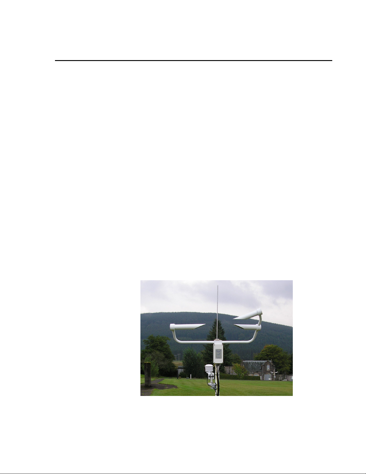
The PWS100 Present Weather Sensor is a laser based sensor capable of
determining precipitation and visibility parameters for automatic weather
stations including road, marine and airport stations. Due to its advanced
measurement technique and fuzzy logic algorithms, the PWS100 can determine
each individual precipitation particle type from accurate size and velocity
measurements and the structure of the received signal.
The system can output visibility and precipitation related weather codes such
as those detailed in the World Meteorological Organisation (WMO) SYNOP
code, those used as part of a METAR weather report and those previously used
by the US National Weather Service (NWS).
Further details of precipitation can be given in terms of drop size distributions
(DSD) and particle size / velocity maps to give better indications of
precipitation intensity. Such distributions can then be used in soil erosion
studies.
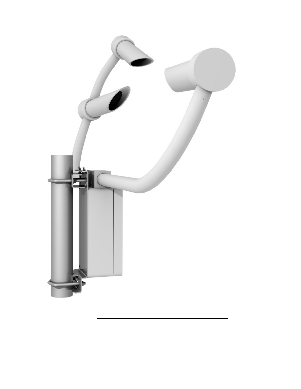
The PWS100 comprises a Digital Signal Processor (DSP) housing unit
connected to a sensor arm, comprising one laser head and two sensor heads.
Each of the sensor heads is 20° off axis to the laser unit axis, one in the
horizontal plane, the other in the vertical plane. The DSP housing is fixed via a
mounting bracket to a mast, though a tripod can be used for temporary sites.
Figure 4-1 shows the PWS100 mounted on a pole.
An optional CS215-PWS temperature and humidity sensor is normally
supplied and plugs directly into the PWS100. That sensor is used to improve
the accuracy of weather coding by the PWS, in particular in respect of
discriminating between snow and rain and also fog/mist and dust.
FIGURE 4-1. PWS100
4-1
Page 18

Section 4. Overview
4-2
Page 19

Section 5. Specifications
5.1 Mechanical Specifications
Measuring Area: 40 cm2 (6.2 in2)
Housing Materials: Iridite NCP conversion coated aluminium
(RoHS compliant) and hard anodized
aluminium. Outer parts also coated with marine
grade paint.
Weight: 8.2 kg (18 lb) excluding power supply /
communications enclosure
Shipping Weight: 20.4 kg (45 lb)
Dimensions: 115 cm × 70 cm × 40 cm (42.3 in × 27.6 in ×
15.8 in)
Mountings: U-bolt mounting to mast or pole with outer
diameter from 1.25 in to 2.07 in
5.2 Electrical Specifications
NOTE
Power Requirements: DSP power 9 to 24 V, (9 to 16 V limit when
using CS215-PWS or other SDI-12 sensors).
Current consumption 200 mA no dew heater or
SDI-12, 1 A with dew heater and SDI-12. The
currents are lower at high supply voltages as
the sensor uses SMPS technology. Hood
heater 24 Vac or dc, 7 A.
It is the responsibility of the user to ensure that any local
regulations, regarding the use of power supplies, are adhered to.
Communication: RS-232, RS-422, RS-485. Baud rate of 300 bps
to 115.2 kbps supported.
Control Unit: Custom DSP board
EMC Compliance: Tested and conforms to BS EN 61326:1998.
Class A device. May cause interference in a
domestic environment.
5-1
Page 20

Section 5. Specifications
5.3 Optical Specifications
5.3.1 Laser Head Specifications
Laser Source: Near-infrared (IR) diode, eye safe Class 1M
Peak Wavelength: 830 nm
Modulation Frequency: 96 kHz
Laser Head Lens Diameter: 50 mm (1.97 in)
5.3.2 Sensor Head Specifications
Receivers: Photodiode with band pass filters
Spectral Response: Maximum spectral sensitivity at 850 nm, 0.62
Sensor Head Lens Diameter: 50 mm (1.97 in)
unit output
A/W (0.6 A/W at 830 nm)
Lens Check Light Source: Near-IR LED
5.4 Environmental Specifications
Standard Operating
Temperature Range: -25° to +50°C
Optional Extended Operating
Temperature Range: -40° to +70°C
Relative Humidity Range: 0 to 100%
IP Rating: IP 66 (NEMA 4X)
5.5 CS215-PWS Specifications
Please refer to the CS215 manual or product brochure for the specifications.
5.6 Measurement Capabilities and Limitations
5.6.1 Visibility Measurements
5-2
Visibility Range: 0 to 20,000 m (0 to 65,620 ft)
Visibility Accuracy: ± 10% (0 to 10,000 m)
Measurement Interval: User selectable from 10 seconds to 2 hours
Page 21

5.6.2 Precipitation Measurements
Particle Size*: 0.1 mm to 30 mm (0.004 in to 1.18 in)
Size Accuracy*: ± 5% (for particles >0.3 mm)
Section 5. Specifications
Particle Velocity: 0.16 ms
-1
to 30 ms-1
Velocity Accuracy*: ± 5% (for particles >0.3 mm)
Types of Precipitation
Detected: Drizzle, rain, snow grains, snow flakes, hail,
ice pellets, graupel (heavily rimed solid
precipitation), freezing rain, freezing drizzle,
mixed (combination of types above)
-1
Rain Rate Intensity Range: 0 to 400 mm h
(M-P Distributed)
Rainfall Resolution: 0.0001 mm
Rain Total Accuracy*: Typically ±10% (accuracy will be degraded for
windy conditions, frozen precipitation, and
very high rainfall rates).
DSD bin sizes: 0.1 mm (diameter) 0.1 ms
-1
(velocity)
Data Output: Raw parameter output (particle size, particle
velocity, signal peak value, signal pedestal
value), WMO SYNOP codes (4680, W
a Wa
precipitation and obscurant type), WMO
METAR codes (4678, W
- precipitation
a Wa
and obscurant type), NWS code, drop size
distribution (DSD) statistics, particle type
distribution, size / velocity intensity maps,
precipitation rate, precipitation accumulation,
visibility range and internal checks
(temperatures, lens contamination, processing
limits).
External Sensors: CS215-PWS supported for temperature / RH
*Accuracy values are for laboratory conditions with reference particles and
visibility standards.
5.6.3 Data Storage and Buffering
The PWS100 has a large internal memory that is split up to store different
types of data. One buffer, the particle buffer, is used to hold raw signal data
captured from the detectors. The size of this buffer and the speed at which it
can be processed is a limit on the maximum rainfall rates the sensor can
measure. For most users, this is not a limitation; if it may be a limitation, please
read the description below.
measurement; SDI-12 compatible sensors
supported.
5-3
Page 22

Section 5. Specifications
The particle buffer is able to hold raw data for 500 typical particles. The
processor is able to process the particles at a rate of 120 particles per second,
typically. This means if more than 120 particles per second fall through the
sample volume of 40 cm
2
the particle buffer will start to fill up. If the rain rate
exceeds 120 particles per second for a prolonged period, the buffer could run
out of space and particles will be lost.
The fact that the processor is running behind real-time and/or particles are
being missed can be monitored in the alarm message which can be selected for
data output.
The particle processor then places data about each particle in the Large Particle
Array (LPA). The LPA is 100000 records long. It uses 5 records every 10
seconds plus a record for every processed particle that passes through the
volume. For example if 20 particles per second are processed then 20.5 records
are used per second. Since 100000 records can be stored, the system can store
100000 / 20.5 = 4878 seconds worth of data in the LPA. The user needs to be
aware of the size of this buffer as it is used to hold data that is processed when
a message is output. The size of the buffer may become a limiting factor if a
very long message interval is selected and rainfall rates are high.
The PWS100 has the capability to store measured data in a buffer called the
message storage buffer, which is 1 MB (1000000 characters) in size. All ASCII
characters including CrLf must be included in any storage calculations. This
buffer stores the user defined messages (see Section 7.5, Message Related
Commands for the types of messages available to the user). A typical message
containing 120 characters can be stored 1000000 / 120 = 8333 times which at
minute intervals for the data output would be over 138 hours worth of storage.
5-4
Page 23
Section 6. Installation
6.1 Location and Orientation
The PWS100 measures environmental variables and is designed to be located
in harsh weather conditions. However there are a few considerations to take
into account if accurate and representative data from a site are to be obtained.
NOTE
The descriptions in this section are not exhaustive. Please refer to
meteorological publications for further information on the
locating of weather instruments.
The PWS100 should be sited in a position representative of local weather
conditions and not of a specific microclimate (unless the analysis of
microclimate weather is being sought).
To give non-microclimatic measurements the PWS100 should be sited away
from possible physical obstructions that could affect the fall of precipitation.
The PWS100 should also be positioned away from sources of heat, electrical
interference and in such a position as to not have direct light on the sensor
lenses.
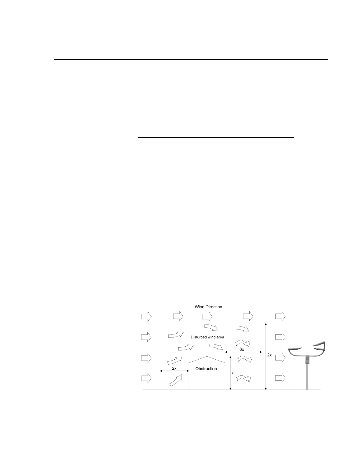
Whenever possible, the PWS100 should be located away from windbreaks.
Several zones have been identified upwind and downwind of a windbreak in
which the airflow is unrepresentative of the general speed and direction. Eddies
are generated in the lee of the windbreak and air is displaced upwind of it. The
height and depth of these affected zones varies with the height and to some
extent the density of the obstacle.
Generally, a structure disturbs the airflow in an upwind direction for a distance
of about twice the height of the structure, and in a downwind direction for a
distance of about six times the height. The airflow is also affected to a vertical
distance of about twice the height of the structure. Ideally, therefore, the
PWS100 should be located outside this zone of influence in order to obtain
representative values for the region (see Figure 6-1).
FIGURE 6-1. Effect of structure on air flow
6-1
Page 24

Section 6. Installation
In order to minimize user interaction with the unit, the PWS100 should be
placed away from sources of contamination, in the case of roadside monitoring,
larger mounting poles can be used. More regular maintenance will be required
when the instrument is placed in areas where contamination is unavoidable or
where measurements may be safety critical.
The orientation of the unit should be such that the horizontal sensor head points
north in the northern hemisphere and south in the southern hemisphere. The
angle of inclination of the second sensor head is such that the deviation from
north/south orientation causes no increase in system noise.
High frequency light sources can lead to increased system noise and hence
erroneous weather classification and so the PWS100 should be positioned in a
location where such interference is minimized. Ideally this should be a
minimum of 100 m from the nearest high frequency light source, with the
sensor heads pointing away from the light source. In any case the sensor heads
should be positioned to be away from any high frequency light source.
Avoid locations where the transmitter is pointing at a light scattering or
reflective surface.
WARNING
When installing the sensor, avoid pointing the laser
housing toward areas where binoculars are commonly
used.
To be at any risk from the laser light source, the operator must look directly
down the beam of light and must be at the same height and in exact alignment
with the sensor. In addition, the beam diverges slightly so the risk decreases
with distance from the sensor.
6.2 Unloading and Unpacking
6.2.1 Unpacking Procedure
Depending on the power and mounting options selected for the PWS100 there
will be up a number of boxes containing the PWS sensor unit, power supply/
external communications enclosure and grounding equipment.
CAUTION
Handle the boxes carefully, taking care not to drop them as
the sensor can be damaged if dropped.
Unpack the boxes carefully and check the contents, ensuring that the contents
match those listed on the packing slip. Carefully remove the items and replace
all packing materials back into the empty boxes and store in case the unit is
required to be repacked for shipping.
6-2
6.2.2 Storage Information
The PWS100 should be stored between -40° to +70°C in a dry place,
preferably with the enclosures securely fastened with desiccant in place. The
optics should be protected from possible accidental damage.
Page 25

6.3 Installation Procedures
6.3.1 Assembling the PWS100
The PWS100 comes as a single unit, with the DSP enclosure attached to the
base of the sensor arms. The PWS100 and power/communication enclosure (if
purchased) are typically mounted to a Campbell Scientific tripod. Usersupplied mounting structures should be strong enough to withstand high winds,
without significant movement.
See the manuals supplied with your tripod for details on how to set up ready
for PWS100 mounting. Tripods need to be firmly secured to a base with the
central pole vertical to ensure correct measurements with the PWS100. See the
relevant tripod or tower manual for further details.
6.3.2 Mounting the PWS100
Section 6. Installation
NOTE
A PWS100 purchased from Campbell Scientific Europe will
have a different mounting bracket.
A pole mounting kit is supplied with the PWS100. This kit includes a DSP
plate, a bracket, two u-bolts, four flat washers, four split washers, and four
nuts. The PWS100 usually comes with the DSP plate attached to it. The
PWS100 mounts onto a Campbell Scientfiic tripod, tower, or a user-supplied
pole with a 1.5 inch (3.81 cm) to 2.1 inch (5.25 cm) outer diameter as follows.
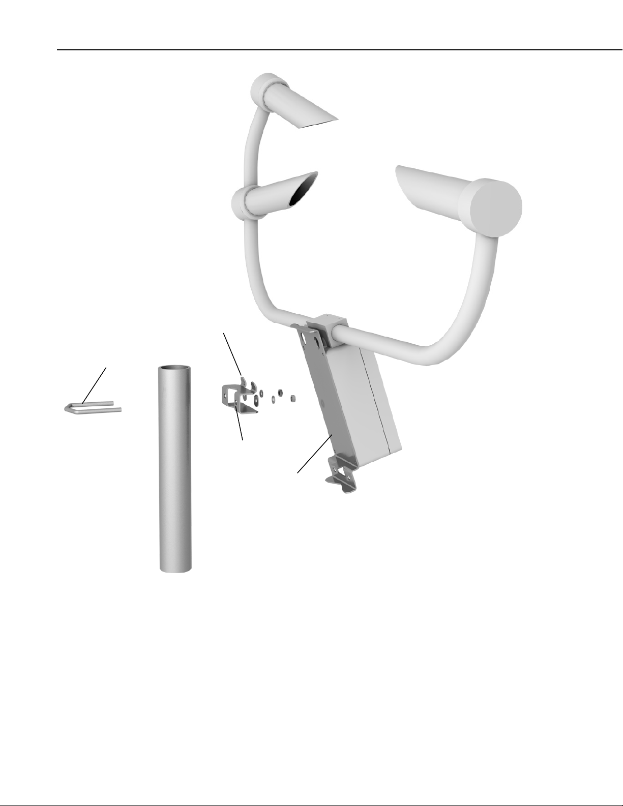
1. Fasten the bracket to the pole using one u-bolt, two flat washers, two split
washers, and two nuts (see Figure 6-2).
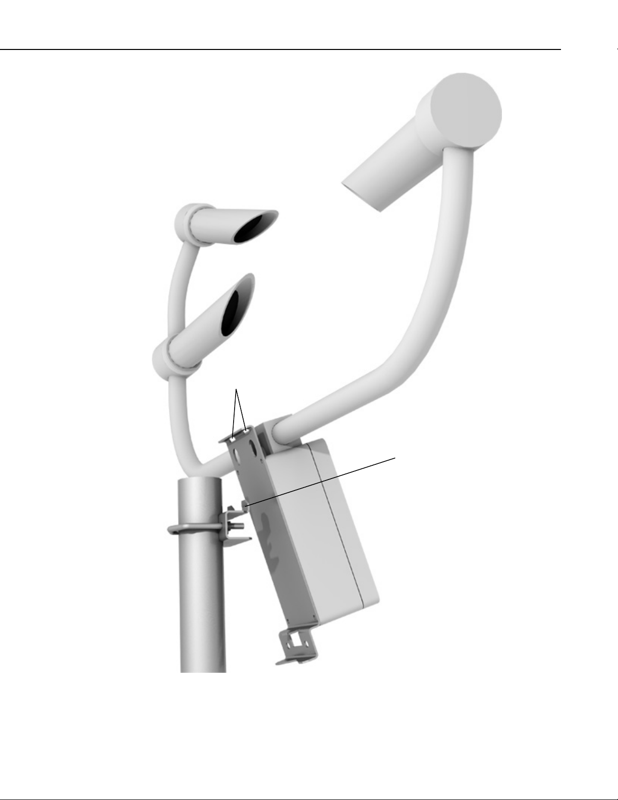
2. Place the DSP plate on the bracket. The tabs of the bracket fit in the
notches at the top of the DSP plate (see Figure 6-3).
3. Fasten the bottom of the DSP plate using the remaining u-bolt, washers,
and nuts (see Figure 6-4).
4. Mount the power supply enclosure if purchased. This enclosure can be
mounted to the same tripod, tower, or user-supplied pole as the PWS100.
Alternatively the power supply can be mounted elsewhere (e.g., on a wall
at some distance from the sensor). The power supply enclosure should be
mounted away from the sensor head to avoid wind flow disturbance or rain
drops bouncing back up into the sensor’s sensing volume.
CAUTION
Take care not to overtighten the nuts on the u-bolts, as it
may be possible to distort and/or damage the bracket or
DSP plate by doing so, and/or the nuts may seize up. Only
tighten the nuts to a degree necessary to hold the PWS100
firmly in place.
6-3
Page 26
Section 6. Installation
Bracket Tab
U-bolt
Bracket
DSP Plate
FIGURE 6-2. Hardware for mounting the top of the DSP plate to a pole
6-4
Page 27
Section 6. Installation
Notches
Bracket Tab
FIGURE 6-3. Placing the PWS100 onto the bracket
6-5
Page 28
Section 6. Installation
6-6
CAUTION
FIGURE 6-4. PWS100 mounted to a mast or pole
Ensure that the PWS100 is mounted according to Figures
6-2 through 6-4. Do not reposition, once fixings are
tightened, by forcing the arms of the unit as this can
damage the unit.
Page 29

6.3.3 Connecting Cables
The sensor unit comes with the DSP control unit fixed to the sensor arm. All
cabling between the sensor heads and the DSP unit is premade. An SDI-12
sensor connection is fixed into the DSP terminal strip. The connection is
terminated with a LEMO socket on the lower face of the DSP housing. This is
primarily wired for the CS215-PWS but is also used with the PWC100
Calibrator. Power, communications and additional sensor connections are to
be routed through the cable glands on the lower face of the DSP housing to the
DSP terminal strip. As a factory default, a power cable and a communications
cable are pre-wired in the unit. The third cable gland will be sealed off by
default but can be used for further external sensor connections or a separate
power cable for the hood heaters (rather than sharing the main power cable).
There should be no need to alter any wiring within the DSP housing and the
housing cover should only be removed periodically to renew desiccant packs or
if any of the hardware switches need to be used. However if cable lengths are
to be changed then these will have to be rewired in the DSP housing. If the unit
remains sealed during operation, the packs should only need replacing once
every 6 months. Replace the desiccant pack in the holder and secure the cover.
6.3.4 Basic Wiring
Section 6. Installation
The PWS100 wiring block is shown on the internal layout diagram in Figure
B-2. Connection points for power and communications are shown in the
diagram. There are two power inputs (one 24V for hood heater and one 12V
for the processor board) one communications connection and two SDI-12 ports
for peripheral connection. For RS-485 communications a 120 Ω termination
resistor may need to be placed across the RTS-B and RX-A connections at
either end of the cable, although this is normally not required for most
installations unless electronic noise interference is prevalent or cable runs are
very long.
A 1K LEMO socket (IP66 rated) is used for connection of a peripheral (often
the CS215-PWS temperature / relative humidity probe). The cable for any
peripheral to be connected to the LEMO socket should be terminated with the
appropriate 4 pin 1K series LEMO plug. Ensure when fitting the peripheral
plug into the socket that the red tabs are aligned.
The power and communications cables are routed through two of the three
cable glands on the base of the PWS100 DSP enclosure. If power and
communications cables are replaced refer to Appendix C.1 and C.2 for further
details.
Figure 6-5 shows the lower face of the DSP enclosure with the cable gland and
LEMO connector positions.
6-7
Page 30

Section 6. Installation
PG9 CABLE GLAND
EARTH GROUND
LEMO 4-PIN
(CONNECTOR FOR
CS215-PWS)
FIGURE 6-5. Underside of DSP enclosure
PG11 CABLE GLAND
(HOOD HEATER)
6-8
Page 31

6.3.5 Desiccant
Section 6. Installation
The desiccant bags should be removed from the plastic bags in which they are
shipped before placing them inside the enclosure. Two 100 g bags of desiccant
are supplied with the PWS100. Desiccant use depends on your application (see
below). The desiccant should be firmly strapped to the DSP cover inside the
PWS electronics enclosure using the strap provided and as shown in Figure
6-6.
FIGURE 6-6. Mounting the desiccant pack on the DSP cover
The second bag of desiccant should be re-sealed in the plastic shipping bag as a
replacement for the initial bag
6.3.6 Communication Options
The communications options are RS-232, RS-422 and RS-485. Baud rate is
selectable between 300 bps and 115.2 kbps. The communications are set on a
series of dip switches on the DSP board itself. The get to the board the DSP
cover must be removed as shown in Figure 6-7. Unscrew the four retaining
screws and carefully lift off to expose the board as shown in Figure 6-8.
6-9
Page 32

Section 6. Installation
FIGURE 6-7. Removal of DSP cover.
6-10
FIGURE 6-8. Exposing the DSP board.
Page 33

Section 6. Installation
The location of the dip switches on the board is shown in Figure 6-9 and the
dip switches themselves are shown in detail in Figure 6-10. The following
settings are available:
PWS100 dip switch settings:-
0 = off; 1 = on.
switch 1 slew rate
0 slow slew rate (default)
1 fast slew rate
switch 2 communication mode
0 RS232 (default)
1 RS485 (note – load resistor may be required – see Section 6.3.6.1)
switch 3 duplex mode
0 full duplex (default)
1 half duplex (RS485 – see Section 6.3.6.1 below)
switch 4-6 serial communication baud rate
switch
654 Baud Rate
000 300
001 1200
010 9600
011 19200
100 38400
101 57600
110 76800
111 115200 (default)
switch 7 reserved for future use (default off)
switch 8 load factory defaults at power up
0 normal operation (default)
1 load factory defaults
6.3.6.1 RS-485 Half-duplex mode
In half duplex mode, the transition from transmits (Tx) to receive (Rx) modes
and vice versa are subject to the following timing rules which may need to be
considered when interfacing other devices:
• The sensor waits for a gap of 1 byte period plus 10 ms without receiving
data before switching from Rx to Tx and echoing/responding.
• Sensor has a 1 millisecond Tx to Rx turn around time.
6-11
Page 34

Section 6. Installation
FIGURE 6-9. DSP board dip switch location (circled)
6-12
FIGURE 6-10. Dip switches (defaults set - 00011100)
Page 35

6.3.7 Installing Power Supply
Power supply connections can be made in the PWS100 24 Vdc/12 Vdc power
supply cabinet using the power cable supplied with the PWS100.
Din rail contacts are mounted inside the power supply enclosure that allows
connection to the two power supplies (see Figure 6-11).
Section 6. Installation
FIGURE 6-11. Labeled DIN-RAIL contacts
6.3.8 Start-Up Testing
On start-up the PWS100 will run internal diagnostic tests and check the status
of any connections to the instrument.
6.3.9 Initial Settings
Initially the PWS100 will be set up with a series of default options set. These
can be altered by entering the command mode of the sensor.
6.3.10 Load Factory Defaults
To load the factory default settings (retaining only the time, date and
calibration values) power down the sensor move dip switch 8 to position 1 and
power up the sensor. Once powered switch dip switch 8 back to position 0.
This removes the password and all other user entered values.
6.3.11 Lubricating the Enclosure Screws
The PWS100 enclosure screws should be lubricated with a suitable anti-seize
grease (often copper loaded) to protect the threads from corrosion. This should
be reapplied when resealing the enclosure at regular intervals, normally after
6-13
Page 36

Section 6. Installation
replacing the desiccant. This is of particular importance if using the sensor in
corrosive or salt laden atmospheres.
6.4 Grounding and Lightning Protection
6.4.1 Equipment Grounding
The present weather sensor must be properly grounded to protect it from
transients and secondary lightning discharges. The PWS100 has a ground lug
on the outside of its enclosure. This ground lug is connected to a tripod’s
grounding system via a 12 AWG copper wire. A 12 AWG copper wire is
included with Campbell Scientific’s tripods or towers.
To ground the system, first install the tripod’s grounding system as described
in the tripod or tower manual. The 12 AWG wire should be fastened to the
tripod or tower’s ground clamp. Route the 12 AWG wire from the clamp to the
PWS100 ground lug. Strip one inch of insulation from each end of the wire
and insert the end of wire into the ground lug and tighten.
6.4.2 Internal Grounding
The DSP enclosure of the unit and associated electronics are grounded through
the power cable assembly. The sensor components are in contact with each
other or have internal copper contacts.
6.4.3 Lightning Rod
Campbell Scientific suggests that a lightning rod is only fitted where there is
significant risk of lightning strike. During rainfall events water can accumulate
and shed from the rod and cause erroneous measurements. The rod itself can
also interfere with the passage of precipitation particles and ice accumulation
can exacerbate the situation.
If required, the lightning rod included with our tripods, UT10 Tower, or
UTGND Ground Kit should be used. The process of mounting the lightning
rod is described in our tripod and tower manuals.
6-14
Page 37

Section 7. Operation
7.1 Introduction
The best way of becoming familiar with the sensor is to setup the sensor and
connect it to a PC running Windows and the Campbell Scientific Present
Weather Viewer program.
This software allows easy setup of the sensor and a graphical display of the
measurements being made. It also provides an easy way of upgrading the
firmware of the sensor. It is not intended to capture or store data on a
permanent basis but is provided as a demonstration, test and setup tool. Brief
details of use of the program are described below. The program includes a
more detailed multi-lingual help system which can be accessed from the Help
menu option once the program is running.
The PWS100 Present Weather Sensor is capable of outputting a range of data,
from single particle parameters, to codes representing those from WMO and
other standard meteorological tables. The sensor is setup with some factory
defined output messages but the user often will need to change these to meet
their own requirements. The setup can be done using either the Present
Weather Viewer program or using a terminal emulator and interacting with the
sensor directly.
7.2 PWS100 Configuration
7.2.1 Using the Present Weather Viewer Program
The latest copy of which can be downloaded from:
www.campbellsci.com/downloads
To use this program install it on your PC. When first run you will be prompted
to chose a connection port and speed. Set these to match the serial port on the
PC being used and the baud rate. With a new sensor the PWS100 address/ID
will be set to zero and there will be no password. With these set you can then
connect icon (top right hand corner) to establish a connection with the sensor.
After the program has checked the sensor setup it will switch to a mode of
displaying data transmitted at regular intervals (one minute by default). The
graphs will then be updated, although they will largely look blank if there is no
precipitation falling. Clicking on the data values and status tab of the display
gives access to basic data which shows the sensor is working OK.
To change settings in the sensor click on the icon near the connection button
which brings up the sensor control panel.
The PWS viewer also provides a simple terminal emulator screen which can be
used to setup the sensor using it’s built in menu system rather than the
graphical interface the viewer provides.
To understand the operation of the sensor and the relevance of the settings in
the graphical interface it is necessary to understand the messages and
7-1
Page 38

Section 7. Operation
configuration options. These are discussed below within the context of setting
up the sensor using a terminal emulator.
7.3 Terminal Mode
In normal operating mode the sensor will respond to a number of “root”
commands, shown in Table 7-1. Those commands allow the configuration of
the sensor in a non-interactive fashion, the polling of data and also switching
the sensor into an interactive user menu mode.
They are accessed via the command TERM PWS_1d Password ↵
Commands are entered in the format ‘Command Pws_1d Password ↵
Command Description
PASSWORD Sets user password
HELP* Gives a list of available commands
OPEN* Activate user menu
TERM Enter command mode
TABLE 7-1. Command Set
CLOSE Exit command mode
MSEND* Poll messages
MSET Set message parameters
HDATA Retrieve historical particle data from sensor
SETPARAM Set weather parameters
FUZZY DIAG* Extra particular information (see Section 7.5.2)
CONFIG View system configuration
SETCONFIG Set system configuration
LOADOS Load a new operating system
DIAGSET Set diagnostic test parameters
DIAG Run diagnostic test
TIME Display or set time and date
RSENSOR Receive remote sensor values (T °C and H %)
RESET Reset hardware
XHMDATA Historic `MSET’ data download using Xmodem
HMDATA Output historic data to the command line
RUNDISC
*These commands are available outside terminal mode.
Rotate the calibration disc for test / demonstration
purposes
7-2
The most commonly used commands are MSEND, HELP and OPEN.
Page 39

Section 7. Operation
In the descriptions which follow ↵ symbolizes the pressing of the ENTER key.
Input parameters in italics should be user-defined characters appropriate for the
command. Unless otherwise stated, all command parameters should be
separated by a space.
To support addressed RS-485 networks, each PWS100 can be assigned an
identifier, shown as Pws_Id below. By default the PWS_Id is set to 0 (zero).
NOTE
When operating at the root level, commands are not echoed back
to the terminal as this mode is intended primarily for polled data
collection and echoed commands will complicate the issue of
decoding the responses sent back from the sensor. Local echo
can be turned on in Hyperterminal if required. Start
Hyperterminal, select the pulldown ‘File’ menu and select
‘Properties’. Click the ‘ASCII setup’ tab and check the ‘Echo
typed characters locally’ checkbox.
7.3.1 Using the Help Command
To list available commands, the HELP command can be used as follows with
the correct PWS100 Pws_Id:
HELP Pws_Id↵
e.g., HELP 0↵
The PWS100 will respond with a list of available commands and their basic
function.
7.3.2 Entering / Exiting the Menu System
The user can enter the menu system by using the OPEN command with the
correct Pws_Id. If a password is set, then it should also be entered. The
command is then as follows:
NOTE
OPEN Pws_Id Password↵
e.g., OPEN 0 campbell↵
The PWS100 will then display the SETUP menu of the menu system
To close the menu system and return the PWS100 to operation, option
9 should be chosen from the SETUP menu (see Figure 7-1). At this
point either option 1 should be chosen to save changes and quit the
menu system, or option 2 should be chosen to lose changes made and
quit the menu system. Option 0 will return the user to the SETUP
menu.
Changes made to the unit calibration and time and date settings
while in the menu system are immediate and as such will remain
changed independent of the quit option chosen from the menu.
7-3
Page 40

Section 7. Operation
NOTE
The data storage function will not store data while the terminal
or menu is active. This means data will be missing during these
periods. To reduce data loss reduce the amount of time that the
terminal or menu are active.
7.3.3 Message Polling
While the menu system or terminal mode are closed, it is possible to poll data
from a suitable set sensor (see Sections 7.4.1 and 7.6.1 for information on how
to set up messages for polling). In order to poll a message the MSEND
command must be used with the correct Pws_Id, stats_period and message_ID.
Statistics are calculated over the stats_period in seconds which completely
overrides any period defined within the message. The message can be either a
fixed or user defined message from 0 to 19. The command for message polling
is as follows:
MSEND Pws_Id stats_period message_ID ↵
e.g., MSEND 0 3600 10↵
In the example given above, the PWS100 will respond with fixed message_ID
10 statistics calculated or sampled over the stats_period of 3600 seconds for
the PWS100 with a Pws_Id of 0. If the stats_period is zero then the statistics
are calculated from the last collection interval. So the polling interval controls
the interval at which statistics are calculated over, up to a maximum of 2 hours.
Setting stat_period to less than 10 seconds will result in repeated data due to
the ten seconds measurement cycle (see Section 8.5).
7.4 PWS100 Menu System
From the command line the use of the OPEN command, as detailed in Section
7.3.2, will initiate the menu system which can be used to set up the operation of
the PWS100.
NOTE
NOTE
If there is no activity for 10 minutes with the menu system open
it will automatically close.
The menu system map is shown in Appendix D. The menu is controlled by
means of numeric selections followed by the enter key. Pressing enter by itself
will return the user to the previous menu. A selection followed by the enter key
will lead to the display of a specific menu or allow a specific parameter value
to be input. Entering an incorrect selection or parameter value will return the
user to the same menu. Pressing the delete key will delete the current entry.
Pressing the escape key will clear the current entry and return to the previous
menu.
Entering the command line (terminal mode) from the menu
system will lead to a loss of all changes made during navigation
of the menu system.
7-4
Page 41

Section 7. Operation
Section 7.4.6 gives further details of how to set up the PWS100 with the
command set in the terminal mode (option 7 from the SETUP menu).
FIGURE 7-1. PWS100 setup menu
7.4.1 Top Menu Options 0, 1 and 2 (Message n)
The options 0, 1 and 2 from the SETUP menu are entitled ‘message 0’,
‘message 1’ and ‘message 2’. These are used to setup the message outputs for
messages with ID 0, 1 and 2. Selecting one of these brings up the MESSAGE
menu as shown in Figure 7-2. Each message allows the user to select message
intervals, modes and fields (option 1).
FIGURE 7-2. Message menu
7-5
Page 42

Section 7. Operation
If option 1 is chosen from the MESSAGE menu then the system will display
the MESSAGE PARAMETERS and FIELDS menu for that message as shown
in Figure 7-3. From here 19 fields can be filled in. Field 0 is the message
interval. This is set in seconds and will be the interval between which output
messages are given. Field 1 is the message mode and fields 2 to 19 are output
parameters which can be user set.
FIGURE 7-3. Message parameters and fields menu
Selecting field 0 brings up the MESSAGE INTERVAL menu shown in Figure
7-4. Here the interval is input. An input of 0 means that the message is polled
(i.e., will be given when the user requests it, either manually or in an automated
fashion using a datalogger).
7-6
FIGURE 7-4. Message interval menu
Page 43

Section 7. Operation
From the MESSAGE PARAMETERS and FIELDS menu if field 1 is chosen
then the MESSAGE MODE menu (see Figure 7-5) will be displayed. Here the
options are to store and output to the serial port (option 1) which is useful for
on screen analysis of real-time data, or store only (option 2) more useful when
logging data.
FIGURE 7-5. Message mode menu
From the MESSAGE PARAMETERS and FIELDS menu if fields 2 to 19 are
chosen then the MESSAGE FIELD menu will be displayed as shown in Figure
7-6. Here an output parameter for that message field can be chosen from a
number of different output parameters as detailed in Table 7-2 and described in
Sections 7.4.1.1 to 7.4.1.40.
TABLE 7-2. Message Field parameters
Message
Parameter Output
Field
0 – 2 User set message types
10 – 19 Fixed messages
20 Average visibility (m)
21 Present weather code (WMO)
22 Present weather code (METAR)
23 Present weather code (NWS)
24 Alarms
25 Fault status of PWS100
30 Average temperature, RH%, wet bulb
31 Minimum and maximum temperature
33 External sensor (Wetness)
7-7
Page 44

Section 7. Operation
TABLE 7-2. Message Field parameters
Message
Parameter Output
Field
34 External sensor (Aux)
40 Precipitation intensity (mmh-1)
41 Precipitation accumulation
42 Drop size distribution bin values (0.1 mm increment
per value)
43 Average velocity (ms-1), average size (mm)
44 Type distribution
45
46
47
Size / velocity map type 1 (20 × 20)
Size / velocity map type 2 (32 × 32)
Campbell Scientific standard size / velocity map (34 × 34)
48 Peak-to-Pedestal ratio distribution histogram
49 Visibility range, in meters, averaged over 10 minutes
100 Internal LED temperatures: upper LED, lower LED
101 Internal detector temperatures: upper, lower
102 Laser hood temperature, laser temperature and laser
current
103 DC offsets: upper, lower, laser
104 Dirty window: upper, lower, laser
105 Battery voltage, hood %, dew %
106 Upper and lower detector differential voltage (mV) and
calibrated visibility voltage (mV)
150 Device s/n, operating system and hardware versions
151 Date and time: day count (from 01/01/2007) HH MM SS
152 Product name “PWS100”
153 Statistics period (s)
154 Watchdog count, maximum particles per second, particles
not processed, time lag
155 Processing statistics
156 Year, month, day
157 Hours, minutes, seconds
158 Averaged corrected visibility voltage (mV) and average
upper head voltage (mV)
159 CRC16-CCITT Checksum
7-8
Page 45

Note that user defined messages cannot make field references to other user
defined messages but can make reference to fixed messages from field 10 to 19
and all other message fields.
7.4.1.1 Message 0 (the Default Output)
User message 0 can be set by setting the Message Field parameters as required
using other message fields from 10 upwards.
By default and after a hardware reset (see Section 6.3.10, Load Factory
Defaults) or a software reset (see Section 7.9.2, Resetting the System) this
outputs the message fields below (in the format as seen in the interactive
menu). These fields have been used as defaults so they give a full display of
the PWS100’s capabilities when used with the Present Weather Sensor Viewer
program.
The user can delete and completely reconfigure this message as required.
(0) Message interval = 60 seconds
(1) Mode = Store and Output
(2) 49 Vis range Av (m) over 10 minutes
(3) 21 WMO code
(4) 22 Metar code
(5) 23 NWS code
(6) 24 Alarms
(7) 25 System fault status 0=pws_ok
1=degraded_performance 2=maintenance
(8) 30 Temp Av (C), RH Samp (%), Wetbulb Av (C)
(9) 31 Temp Max (C), Temp Min (C)
(10) 40 Precipitation Intensity (mm / hour)
(11) 41 Precipitation accumulation (mm)
(12) 42 Particle size distribution (300 values 0.1 to 30mm)
(13) 43 Particle Av velocity (m/s), Av size (mm)
(14) 44 Particle type distribution (fd, d, fr, r, sg,
sf, ip, h, g, e, u)
(15) 47 Size and velocity map Campbell 34x34
(16) 48 Ped ratio distribution (50 values 1.0 to 6.0)
(17) 156 Date (year, month, day)
(18) 157 Time (hours, minutes, seconds)
(19) 159 CRC16-CCITT
Section 7. Operation
Note that in the default message, the start and end characters (STX/ETX) are
included in the message – see “Output options” described in Section 7.4.3.
7.4.1.2 Message Field 1 and 2 User Defined Message
These user messages are set in the same way as message 0 but are cleared and
do not output as default after a master reset.
7-9
Page 46

Section 7. Operation
7.4.1.3 Message Field 10 To 19 Fixed Messages
7.4.1.4 Message Field 20 Visibility Range (m)
7.4.1.5 Message Field 21 Present Weather Code (WMO)
7.4.1.6 Message Field 22 Present Weather Code (METAR)
7.4.1.7 Message Field 23 Present Weather Code (NWS)
No fixed messages have been defined yet. The user cannot change the fixed
messages.
This field will output the average visibility range (m) calculated over the
Message_Interval defined.
This field will output the Present Weather Code (WMO) calculated over the
Message_Interval defined.
This field will output the Present Weather Code (METAR) calculated over the
Message_Interval defined.
This field will output the Present Weather Code (NWS) calculated over the
Message_Interval defined.
7.4.1.8 Message Field 24 Alarms
This field will output the Alarms. The alarms are output as a string of 16 ‘0’s
and ‘1’s delimited with spaces, for example 1 1 1 1 1 1 1 1 1 1 1 1 1 1 1 1.
Each alarm has the following definition starting from the left hand side:
1. Visibility range less than alarm 1 trigger point set by user. The factory
default is 5 km.
2. Visibility range less than alarm 2 trigger point set by user. The factory
default is 1.5 km.
3. Visibility range less than alarm 3 trigger point set by user. The factory
default is 0.5 km.
4. Laser drive current greater than 80 mA. This may indicate the laser is
failing or recalibration is required.
5. Power supply voltage for dsp less than 11 V.
6. Laser window needs cleaning. There is sufficient build up on the
window that if not cleaned could reduce accuracy.
7. Upper detector window needs cleaning. There is sufficient build up on
the window that if not cleaned could reduce accuracy.
8. Lower detector window needs cleaning. There is sufficient build up on
the window that if not cleaned could reduce accuracy.
7-10
9. DC voltage of laser dirty window detector greater than 1.5 V. This can
be caused by sun directly shining into lens or a pws fault.
Page 47

Section 7. Operation
10. DC voltage of upper detector greater than 1.5 V. This can be caused
by sun directly shining into lens or a pws fault.
11. DC voltage of lower detector greater than 1.5 V. This can be caused
by sun directly shining into lens or a pws fault.
12. Particle processor is unable to process all particles due to limited time
and buffer resources. Particles are missed and data could be
inaccurate. This alarm may activate when there are 120 or more
particles per second going through the volume, sustained for a period
that fills all available space in the buffers.
13. Particle processor lags real time by more than 5% of the user
requested statistics interval.
14. Particle stripper is unable to process all particles due to limited time
and buffer resources. Particles are missed and data will be inaccurate.
This alarm may activate if there are more than ~150 particles per
second going through the volume.
15. Reserved for future use. Outputs ‘0’.
16. Reserved for future use. Outputs ‘0’.
7.4.1.9 Message Field 25 Fault Status of the PWS100
This field will output the fault status of the PWS100. The value output is from
0 to 4. 0 = no fault, 1 = Possible degraded performance, 2 = Degraded
performance, 3 = Maintenance required, 4 = Laser fault.
7.4.1.10 Message Field 30 External Sensor Temperature, RH% and Wetbulb
This field will output the averaged temperature (°C), sampled relative humidity
and averaged wetbulb temperature (°C) calculated over the Message_Interval
defined.
7.4.1.11 Message Field 31 External Sensor Maximum and Minimum Temperature
This field will output the maximum and minimum temperature (°C) calculated
over the Message_Interval defined.
7.4.1.12 Message Field 33 External Sensor Wetness
This field will output the sampled wetness (0-100%).
7.4.1.13 Message Field 34 External Sensor Aux
This field will output the sampled auxiliary sensor output. Such an auxiliary
sensor needs to be defined.
7.4.1.14 Message Field 40 Precipitation Intensity
This field will output the precipitation intensity (mm / hour) calculated over the
Message_Interval defined.
7-11
Page 48

Section 7. Operation
NOTE
The PWS100 only measures particles / visibility 90% of the time
so precipitation intensity is scaled appropriately.
7.4.1.15 Message Field 41 Precipitation Accumulation
This field will output the precipitation accumulation (mm) calculated over the
Message_Interval defined.
NOTE
The PWS100 only measures particles / visibility 90% of the time
so precipitation totals are scaled appropriately.
7.4.1.16 Message Field 42 Drop Size Distribution
This field will output the drop size distribution table which is output as 300
values, starting with the 0 to 0.1 mm bin, in steps of 0.1 mm up to 30 mm. This
is calculated over the Message_Interval defined.
7.4.1.17 Message Field 43 Average Velocity (ms
-1
) and Average Size (mm)
This field will output the average velocity and average size values ignoring any
particle type classifications.
7.4.1.18 Message Field 44 Type Distribution
This field will output the type distribution which is a series of 11 values for
each particle type which shows the number of each type of particle classified.
The order of the output is: drizzle, freezing drizzle, rain, freezing rain, snow
grains, snow flakes, ice pellets, hail, graupel, error, unknown.
7.4.1.19 Message Field 45 Size / Velocity Type Map 1 (20 x 20)
This field will output a size and velocity map with the following classes:
Particle diameter class
Class Diameter [mm] Class width [mm]
*1 =>0.00 0.24
2 =>0.24 0.12
3 =>0.36 0.14
4 =>0.50 0.25
5 =>0.75 0.25
6 =>1.00 0.25
7 =>1.25 0.25
8 =>1.50 0.25
9 =>1.75 0.25
10 =>2.00 0.50
11 =>2.50 0.50
12 =>3.00 0.50
13 =>3.50 0.50
14 =>4.00 0.50
7-12
Page 49

Section 7. Operation
15 =>4.50 0.50
16 =>5.00 0.50
17 =>5.50 0.50
18 =>6.00 0.50
19 =>6.50 0.50
20 =>7.00 93.00
Particle speed class
Class Speed [m/s] Class width [m/s]
1 =>0.0 0.2
2 =>0.2 0.2
3 =>0.4 0.2
4 =>0.6 0.2
5 =>0.8 0.2
6 =>1.0 0.4
7 =>1.4 0.4
8 =>1.8 0.4
9 =>2.2 0.4
10 =>2.6 0.4
11 =>3.0 0.4
12 =>3.4 0.8
13 =>4.2 0.8
14 =>5.0 0.8
15 =>5.8 0.8
16 =>6.6 0.8
17 =>7.4 0.8
18 =>8.2 0.8
19 =>9.0 1.0
20 =>10.0 90.0
7.4.1.20 Message Field 46 Size / Velocity Type Map 2 (32 x 32)
This field will output a size and velocity map with the following classes:
Particle diameter class
Class
Average Diameter
[mm]
1 0.060 0.12
2 0.180 0.12
3 0.300 0.12
4 0.420 0.12
5 0.540 0.12
6 0.665 0.13
Class width [mm]
7-13
Page 50

Section 7. Operation
7 0.795 0.13
8 0.925 0.13
9 1.055 0.13
10 1.185 0.13
11 1.375 0.25
12 1.625 0.25
13 1.875 0.25
14 2.125 0.25
15 2.375 0.25
16 2.750 0.50
17 3.250 0.50
18 3.750 0.50
19 4.250 0.50
20 4.750 0.50
21 5.500 1.00
22 6.500 1.00
23 7.500 1.00
24 8.500 1.00
25 9.500 1.00
26 11.000 2.00
27 13.000 2.00
28 15.000 2.00
29 17.000 2.00
30 19.000 2.00
31 21.500 3.00
32 =>23.000 77.00
Particle speed class
7-14
Class Average Speed [m/s] Class width [m/s]
1 0.05 0.1
2 0.15 0.1
3 0.25 0.1
4 0.35 0.1
5 0.45 0.1
6 0.55 0.1
7 0.65 0.1
8 0.75 0.1
9 0.85 0.1
Page 51

Section 7. Operation
10 0.95 0.1
11 1.10 0.2
12 1.30 0.2
13 1.50 0.2
14 1.70 0.2
15 1.90 0.2
16 2.20 0.4
17 2.60 0.4
18 3.00 0.4
19 3.40 0.4
20 3.80 0.4
21 4.40 0.8
22 5.20 0.8
23 6.00 0.8
24 6.80 0.8
25 7.60 0.8
26 8.80 1.6
27 10.40 1.6
28 12.00 1.6
29 13.60 1.6
30 15.20 1.6
31 17.60 3.2
32 =>19.20 80.8
7.4.1.21 Message Field 47 Campbell Scientific Standard Size / Velocity Map (34 x 34)
This field will output the standard Campbell Scientific size and velocity map
with the following classes:
Particle diameter class
Class Diameter [mm] Class width [mm]
1 =>0.00 0.1
2 =>0.10 0.1
3 =>0.20 0.1
4 =>0.30 0.1
5 =>0.40 0.1
6 =>0.50 0.1
7 =>0.60 0.1
7-15
Page 52

Section 7. Operation
8 =>0.70 0.1
9 =>0.80 0.1
10 =>0.90 0.1
11 =>1.00 0.2
12 =>1.20 0.2
13 =>1.40 0.2
14 =>1.60 0.2
15 =>1.80 0.2
16 =>2.00 0.4
17 =>2.40 0.4
18 =>2.80 0.4
19 =>3.20 0.4
20 =>3.60 0.4
21 =>4.00 0.8
22 =>4.80 0.8
23 =>5.60 0.8
24 =>6.40 0.8
25 =>7.20 0.8
26 =>8.00 1.6
27 =>9.60 1.6
28 =>11.20 1.6
29 =>12.80 1.6
30 =>14.40 1.6
31 =>16.00 3.2
32 =>19.20 3.2
33 =>22.40 3.2
34 =>25.60 74.4
Particle speed class
7-16
Class Speed [m/s] Class width [m/s]
1 =>0.00 0.1
2 =>0.10 0.1
3 =>0.20 0.1
4 =>0.30 0.1
5 =>0.40 0.1
6 =>0.50 0.1
7 =>0.60 0.1
8 =>0.70 0.1
9 =>0.80 0.1
10 =>0.90 0.1
Page 53

Section 7. Operation
11 =>1.00 0.2
12 =>1.20 0.2
13 =>1.40 0.2
14 =>1.60 0.2
15 =>1.80 0.2
16 =>2.00 0.4
17 =>2.40 0.4
18 =>2.80 0.4
19 =>3.20 0.4
20 =>3.60 0.4
21 =>4.00 0.8
22 =>4.80 0.8
23 =>5.60 0.8
24 =>6.40 0.8
25 =>7.20 0.8
26 =>8.00 1.6
27 =>9.60 1.6
28 =>11.20 1.6
29 =>12.80 1.6
30 =>14.40 1.6
31 =>16.00 3.2
32 =>19.20 3.2
33 =>22.40 3.2
34 =>25.60 74.4
7.4.1.22 Message Field 48
This field outputs a histogram which contains the number of particles counted
within the measurement period that have a given peak-to-pedestal ratio (see
Section 8.6 – this gives a measure of the number of crystalline particles). This
is a histogram of 50 bins for ratios for 1.0 to 6.0 in steps of 0.1.
Note that the ratios for particles less that 0.5 mm in size are not accurate so are
not included in this histogram. The total number of particles in this histogram
can therefore be less than the total particles detected.
7.4.1.23 Message Field 49 Visibility (m), 10 minute average
This field will output the average visibility range (m) calculated over the
previous 10 minutes, independent of the message interval – this is a 10 minute
rolling average.
7-17
Page 54

Section 7. Operation
7.4.1.24 Message Field 100 Upper, Lower LED temperature
7.4.1.25 Message Field 101 Upper, Lower Detector Temperature
7.4.1.26 Message Field 102 Laser Hood, Laser Temperature and Laser Drive Current
7.4.1.27 Message Field 103 Laser, Upper, Lower Detector DC Voltage Offsets
7.4.1.28 Message Field 104 Laser, Upper and Lower Dirty Window Detector
This field will output the sampled internal upper and lower LED temperatures
(°C).
This field will output the sampled internal upper and lower detector
temperatures (°C).
This field will output the sampled internal laser hood temperature (°C), laser
temperature (°C), and laser drive current (mA).
This field will output the sampled internal laser dirty window detector, upper
and lower detector DC offsets (mV).
This field will output the sampled internal laser, upper and lower dirty window
detector voltage levels (mV).
7.4.1.29 Message Field 105 DSP PSU Voltage, Hood and Dew Heater % Duty
This field will output the sampled DSP PSU voltage (V), hood and dew heater
duty (0 to 100%)
7.4.1.30 Message Field 106 Upper, Lower Detector Differential Voltage, Calibrated Visibility mV
This field will output the sampled upper, lower detector differential voltage
(mV) and the calibrated visibility (mV).
7.4.1.31 Message Field 150 Serial Number, Operating System and Hardware Version
This field will output the system serial number, operating system and hardware
version numbers.
7.4.1.32 Message Field 151 Day Count, Hours, Minutes, Seconds
This field will output the day count (from 01/01/2007), hours, minutes and
seconds.
7.4.1.33 Message Field 152 Product Name
7-18
This field will output the product name PWS100.
7.4.1.34 Message Field 153 Statistics Period
This field will output the statistics period in seconds.
Page 55

Section 7. Operation
7.4.1.35 Message Field 154 Watchdog Count, Maximum Particles Per Second, Particles
Not Processed, Time Lag
This field will output a watchdog count which indicates the number of resets of
the system due to error, the maximum number of particles stripped per second
over the measurement interval, the number of particles stripped in real time but
not processed and a time lag in seconds indicating how far behind processing
has got at some point during the measurement interval.
7.4.1.36 Message Field 155 Processing Statistics
Shows the statistical distribution of particle processing methods used on each
particle and is generally intended for debug purposes only; contact Campbell
Scientific for details.
7.4.1.37 Message Field 156 Year, Month, Day
This field will output the year, month, and day.
7.4.1.38 Message Field 157 Hours, Minutes, Seconds
This field will output hours, minutes, and seconds.
7.4.1.39 Message Field 158 Averaged Corrected Visibility Voltage and Averaged Upper
Head Voltage
Shows the average voltage (mV) value corresponding to the corrected visibility
value (i.e., adjusted for atmospheric conditions) and the average mV value for
the upper head.
7.4.1.40 Message Field 159 Output a CCITT CRC-16 (checksum) of the message
This outputs a two byte checksum in hex format (four ASCII characters). This
is normally included at the end of a message to allow the validity of the
message to be checked. The CRC some not include the checksum itself or
STX/ETX characters.
7.4.1.41 Message Field Error
If “Error - message field nnn not valid” is output then this indicates the
message you have defined has an invalid field which is not in the list above.
You must go and check / re-edit your message definition.
7-19
Page 56

Section 7. Operation
FIGURE 7-6. Message field menu
Choosing option 0 on the MESSAGE FIELD menu will display more output
parameter options. Choosing option 999 will delete the field (note that
subsequent fields already selected shift up to fill the gap in the fields).
Choosing option 1000 + field number will insert the chosen parameter in the
field selected and shift subsequent filled fields down one field.
Also available on the MESSAGE menu is the option to delete the message
(option 2). If the message is to be deleted the DELETE MESSAGE menu (see
Figure 7-7) will be shown. Choosing option 1 will not delete the message and
will return the user to the previous menu; option 2 will delete the message. If a
message is deleted a new message can be created for that message ID.
Messages not deleted will retain their message ID. Therefore if all messages
are set and message 1 is deleted then messages 0 and 2 are still active and will
still be output. Message 1 can be redefined if required.
7-20
Page 57

FIGURE 7-7. Delete message menu
Section 7. Operation
7.4.2 Top Menu Option 3 (Set Time and Date)
Choosing option 3 from the SETUP menu brings up the TIME AND DATE
menu (see Figure 7-8). On this menu it is possible to set the time and / or date
for the PWS100. To change the time alone enter it as hh:mm:ss, for example
16:30:00. To change the date alone enter it as yyyy/mm/dd), for example
2007/02/04. To set the time and date simultaneously enter both of these
parameters on the same line, for example 16:30:00 2007/02/04. Leading
zeroes are not required on the values but the colons (:) and forward slashes (/)
are and a space is required between the time and date values.
FIGURE 7-8. Time and date menu
7-21
Page 58

Section 7. Operation
7.4.3 Top Menu Option 4 (Configuration)
Choosing option 4 from the SETUP menu brings up the CONFIGURATION
menu (see Figure 7-9). From this menu the basic configuration of the sensor is
set.
FIGURE 7-9. Configuration menu
Option 1 of the configuration menu gives the PWS100 ID menu (Figure 7-10).
Here a PWS100 ID can be set. This is effectively the station address which is
required on any communication with the PWS100. If the PWS100 is on a
network with more than one PWS100 then each station should have its own
PWS100 ID. The default PWS100 ID is zero.
7-22
Page 59

FIGURE 7-10. PWS100 ID menu
Section 7. Operation
Option 2 of the configuration menu gives the TRH PROBE TYPE menu (see
Figure 7-11). Choose the correct temperature / relative humidity probe that is
connected to the PWS100 from the list given.
FIGURE 7-11. TRH probe menu
Selecting probe type 2 configures the sensor to expect a temperature and
humidity reading to be sent to it from a remote system using the RSENSOR
command.
7-23
Page 60

Section 7. Operation
Option 3 of the configuration menu gives the WETNESS PROBE TYPE menu
(see Figure 7-12). Choose the correct wetness probe that is connected to the
PWS100 from the list given.
FIGURE 7-12. Wetness probe menu
Option 4 of the configuration menu gives the AUX PROBE TYPE menu (see
Figure 7-13). Choose the correct auxiliary probe that is connected to the
PWS100 from the list given.
7-24
FIGURE 7-13. Aux probe menu
Page 61

Section 7. Operation
Option 5 of the configuration menu gives the HOOD HEATER
TEMPERATURE menu (see Figure 7-14). The value that is to be set needs to
be between 0° and 50°C. The hood temperature is maintained by the system at
the value set.
FIGURE 7-14. Hood heater temperature menu
Option 6 of the configuration menu gives the DEW HEATER MODE menu
(see Figure 7-15). The dew heaters can be set to on, off or auto. Auto mode
turns the heaters on, except when main hood heaters are set to heat.
FIGURE 7-15. Dew heater mode menu
7-25
Page 62

Section 7. Operation
Option 7 of the configuration menu gives the OUTPUT MODE menu (Figure
7-16). This refers to the use of packetized output. The message framing is done
by STX (ASCII character 02) and ETX (ASCII character 03); these act as start
and end delimiters. The default value is 1 (STX / ETX on). These framing
characters are useful for programmers writing code to pick up data coming
from a sensor outputting data asynchronously to the device collecting it.
FIGURE 7-16. Output mode menu
Option 8 of the configuration menu gives the initial warning screen for the
calibration procedure (Figure 7-17). Unless the correct procedure is followed
and calibration entries are correctly input the PWS100’s performance can be
seriously degraded. In order to perform a calibration, the PWC100 calibration
unit is required, which affixes to the PWS and performs several checks of the
PWS100. This unit is connected via the LEMO socket of the PWS100 and
automatically provides values to the PWS100 system which can be used to
alter the calibration.
See the PWC100 calibrator manual for further instructions on how to run the
calibration device. The device itself can be run at any time during the operation
of the PWS100. It then provides size, velocity and visibility calibration values
which can be checked and accepted by the user using the PWS100 menu
system described below.
In order to proceed with the calibration routine confirm must be typed followed
by the return key.
7-26
Page 63

Section 7. Operation
FIGURE 7-17. Calibration warning screen
Once confirm is typed followed by the return key, the CALIBRATION top
menu (see Figure 7-18) appears. The options available to the user are: 0 to
view and enter the calibration disc constants, and 1 to view and adjust the
PWS100 calibration.
FIGURE 7-18. Calibration top menu
Selecting option 0 on the CALIBRATION top menu will bring up the
CALIBRATION DISC CONSTANTS menu (see Figure 7-19). The following
can then be entered (each followed by the return key); the calibration disc serial
number, which identifies the specific disc for traceability; the size value; the
visibility value. The velocity value is fixed by the PWC100 calibrator unit and
is not a function of the disc and so this value is fixed and not user enterable.
7-27
Page 64

Section 7. Operation
FIGURE 7-19. Calibration disc constants menu
Selecting option 1 on the CALIBRATION top menu will bring up the VIEW /
ADJUST CALIBRATION menu (see Figure 7-20). On this menu the latest
calibration values will be evident in the left hand column of values headed
latest. Selecting option 0 on the VIEW / ADJUST CALIBRATION menu will
return the user to the previous menu without invoking any calibration changes.
Selecting option 1 from the VIEW / ADJUST CALIBRATION menu will
allow the user to update the calibration values for velocity, size and visibility.
If the values are in the target range then all is correct with the sensor. If values
are out then there may be a problem, such as dirty windows on the PWS100, an
error with the PWC100 calibrator, or some further problem with the PWS100
that may need investigation. In this instance, ensure that the PWC100
calibrator is working as described in the PWC100 calibrator manual, and
ensure that all lenses are clear of dirt or fingerprints. Place the PWS100 in a
suitable location and attempt the calibration again. If a problem persists then it
may be necessary to contact Campbell Scientific for further diagnostics.
7-28
NOTE
The calibration should only be carried out during nonprecipitation conditions and during clear atmospheric conditions
(>10 km visibility).
Page 65

FIGURE 7-20. View / adjust calibration menu
Section 7. Operation
NOTE
Option 9 of the configuration menu gives the TERMINAL MODE menu (see
Figure 7-21). Choose whether CRC16-CCITT checksum verification is
required.
When terminal mode is set to 1 all terminal commands need a
CRC. For example “open 0;d2d5” a semi-colon is used to
indicate start of CRC in 4 byte ASCII hex. The CRC is
calculated either from the start of new line or after a [STX] up to
but not including the semicolon. ETX can follow the CRC if
required. The valid CRC can be read back for any command if
the CRC after the semi-colon is replaced with four `?’. For
example “open 0;????” the response will
be
[CRLF]CRC>D2D5<CRC[CRLF] so d2d5 is the
CRC.
FIGURE 7-21. Terminal mode menu
7-29
Page 66

Section 7. Operation
Option 10 of the configuration menu gives the PSU SHUT DOWN VOLTAGE
menu (Figure 7-22). Enter the PSU input voltage level below which the
PWS100 will enter low power mode. Enter `0.0’ to disable this feature
(default).
FIGURE 7-22. PSU shut down voltage menu
NOTE
This feature is usually used to protect batteries from deep
discharge. There is a hysteresis of 0.9V applied. For example, if
the PWS100 goes into low power mode at 10V it will return to
normal operation when the voltage rises to 10.9V. Current will
be limited to about 120 mA at 9V. Communications are still
possible and a message “PSU voltage too low nn.n”, where nn.n
is the supply voltage, will be output every 60 seconds.
7.4.4 Top Menu Option 5 (Password)
Choosing option 5 from the SETUP menu brings up the PASSWORD menu
(see Figure 7-23). Pressing enter deletes the password. To set a password, type
up to 10 alpha-numeric characters and press enter.
7-30
FIGURE 7-23. Password menu
Page 67

Section 7. Operation
7.4.5 Top Menu Option 6 (Weather and Alarm Parameters)
Choosing option 6 from the SETUP menu brings up the WEATHER AND
ALARM PARAMETERS menu (see Figure 7-24). This menu allows for the
setup of the visibility range alarms, snow water content factor and the mixed
precipitation thresholds.
FIGURE 7-24. Weather parameters menu
There are three visibility alarms, each of which is set separately by selecting 1,
2, or 3, followed by enter on the WEATHER PARAMETERS menu. Selection
of one of the visibility range alarms brings up the individual alarm menu
(Figure 7-25). Select an alarm range from 0 to 50000 m noting that the
PWS100 visibility measurement is currently capped at 20000 m and so values
set above this cap will set an alarm that is never triggered. These alarms are
triggered and stored in the sensor and can be output as part of a message or
used as flags as part of a monitoring system.
FIGURE 7-25. Visibility range alarm menu
7-31
Page 68

Section 7. Operation
The snow water content scaling factor (SWCF) can be adjusted by choosing
option 4 on the WEATHER PARAMETERS menu. This will bring up a line
asking for a value.
Depending on atmospheric conditions likely to be encountered, a wide range of
snow water content figures can be observed dependant on the bulk density of
the particle. Particle bulk density depends on the structure of the particle (e.g.,
whether it is dendritic, columnar or plate-like as the surrounding air or
encapsulated air occupies some of the particle space). The conversion from a
measurement of size (which in itself is not precise for irregular snowflakes)
and water content can at best be considered approximate.
The PWS100 assumes a relationship between snow flake size and bulk density
published in the literature (Brandes, E. A., K. Ikeda, G. Zhang, M. Schönhuber,
and R. M. Rasmussen, 2007: A statistical and physical description of
hydrometeor distributions in Colorado snow storms using a video disdrometer.
J. Appl. Meteor., 46, 634−650). That equation and the values it assumes for
other identified particle types are given in Table 7-3. The equation for
snowflakes has the scaling factor for snow water content that can be adjusted to
suit local conditions. Entering a value of 1 assume this relationship is correct.
For example, if the snow at the site of installation is typically more dense and
wet (as is common in temperate climates) a higher scaling factor may be
needed.
TABLE 7-3. Assumed bulk density of various
particle types.
Particle Type Bulk Density assumed
Liquid 1.0 g cm-3
Graupel 0.6 g cm-3
Snow grain 0.4 g cm-3
Ice pellet 0.7 g cm-3
Hail 0.8 g cm-3
Snow Flake SWCF* 0.178*D
(D is the flake diameter in mm)
-0.922
g cm
-3
This figure should not be confused with equivalent water to snow depth
calculations which require further knowledge of packing structures, wind
effects, ground temperature, ground type and a myriad of other parameters
related to snow depth. The ratio of water accumulation to snow depth will be
lower than the snow water content figure and is typically in the order of 0.1
(i.e., the snow pack is 10 times deeper than the water accumulation of the
melted snow pack).
7-32
NOTE
Changing the snow water content parameter will also affect the
determination of precipitation intensity, which is defined by
water equivalent precipitation rates. See 8.6.2 and Appendix A
for more details.
Page 69

FIGURE 7-26. Snow water content adjustment
Section 7. Operation
The mixed precipitation threshold value can be adjusted by choosing options 58 on the WEATHER PARAMETERS menu. This will bring up a line asking
for a value between 0 to 1. A value of 0 means there is no threshold for mixed
precipitation – a single other type of particle in a specific event will give rise to
a mixed event, therefore mixed events are highly likely; and may easily be
caused by the occasional erroneous particle classification. A value of 1 means
an equal number of two types will have to be observed to trigger a mixed
event, therefore mixed events are highly unlikely. A setting of 0.5 means that a
second precipitation type needs to be 50% or more of the most common type to
be distinguished as a mixed event.
Four thresholds are given to allow maximum flexibility and to allow the sensor
to be setup to match local observer practise (which varies).
Option 5 controls the threshold for mixed events between two types of liquid
precipitation (e.g., rain and drizzle).
Option 6 controls the threshold for mixed events when a liquid type is the
dominant particle type and a solid is the next most prevalent particle type (e.g.,
when it is raining and snow flakes are detected). Observers are typically more
sensitive to reporting this as a mixed event than for rain/drizzle as occasional
snow flakes are easy to see.
Option 7 controls the threshold for mixed events when a solid type is the
dominant particle type and a liquid is the next most prevalent particle type
(e.g., when it is snowing but changing to rain).
Option 5 controls the threshold for mixed events between two types of solid
precipitation (e.g., snow and snow pellets).
7-33
Page 70

Section 7. Operation
7.4.6 Top Menu Option 7 (Terminal)
FIGURE 7-27. Mixed precipitation threshold adjustment
Choosing option 7 from the SETUP menu brings up the TERMINAL screen
(see Figure 7-28). Pressing any key brings up the terminal as described in
Section 7.3.
7-34
FIGURE 7-28. Terminal active screen
7.4.7 Top Menu Option 8 (Info)
Choosing option 8 from the SETUP menu brings up the INFORMATION
menu (see Figure 7-29). This shows various parameters for the PWS100
system. The software version shows the current operating system number
which may be required in communications with Campbell Scientific about the
PWS100. The watchdog shows errors that have occurred since the installation
Page 71

Section 7. Operation
of the operating system or a hardware reset. The SDI-12 values of temperature
and relative humidity will be -999.00 if no such information is available such
as when no probe is connected to the SDI-12 port. The diagnostic mode shows
two values. The first value is the flag for the fuzzy diagnostic mode (0 or 1);
see Section 7.5.2, Retrieving Historical Data for more information. The second
value indicates the connection status of the calibration unit, 0 shows that the
unit is not connected and 1 shows that it is connected.
FIGURE 7-29. Information menu
7.4.8 Top Menu Option 9 (Done)
Choosing option 9 from the SETUP menu brings up the DONE menu (see
Figure 7-30). Here changes made can be saved before quitting (option 1) or lost
before quitting (option 2). Alternatively option 0 returns to the main menu.
7-35
Page 72

Section 7. Operation
FIGURE 7-30. Done menu
7.5 Message Related Commands
Messages can be set for a variety of output types, including fixed standard
types and user defined types. The system can be set up to send automated
messages at user defined intervals, or can be used as a user polled system.
7.5.1 Automatic and Polled Message Sending
While the command mode is closed, the PWS100 will operate by sending data
output as set by the user in either automatic or polled modes (see Section 7.3.3,
Message Polling for a description of the manual data polling command).
To define the output parameters and fields, use the MSET command with the
Message_ID, Message_Interval, Message_Mode and Message_Fields
parameters as follows:
MSET Message_ID Message_Interval Message_Mode
Message_Fields ↵
e.g., MSET 0 3600 0 105 106↵
In order to ensure that output is as required, the Message_ID,
Message_Interval, Message_Mode and Message_Fields parameters must be
defined.
7-36
Three Message_IDs 0, 1 and 2 can be defined to provide the scope for different
output types to be given at different time intervals (e.g., Message_ID 0 can be
defined with a 15 second interval, whereas Message_ID 1 can have a 60 second
interval). Then every 15 seconds the message defined by Message_ID 0 will be
output, additionally every 60 seconds the message defined by Message_ID 1
will be output. Each Message_ID should be defined as a separate command.
Page 73

Section 7. Operation
The Message_Interval parameter must also be defined from 0 second to 32767
seconds which is the rate at which the system will display the output message
and the period which statistics are calculated over (the factory and reset default
for ID 0 is 60 seconds). If the Message_Interval is 0 then it will set the
message polling mode (see Section 7.3.3, Message Polling for a description of
the manual data polling command). Setting the Message_Interval to less than
10 seconds will result in repeated data due to the 10 second measurement cycle
in the sensor (see Section 8.5).
The Message_Mode defines special functions and can be set to either 0 or 1.
Setting Message_Mode to 0 allows output to the serial port and stores the
‘MSET’ data history. Setting the Message_Mode to 1 prevents the output to the
serial port but stores the ‘MSET’ data. For message polling, mode the
Message_Mode should be set to 0.
By default (factory set and after reset of the system) the Message_Field
parameter for message_ID 0 is set up as described in Section 7.4.1.1, which is a
combination of message types. If no message field parameters are set, then no
output will be given, thus a particular ID can be cleared by using the above
method.
There are many fixed message types which are detailed elsewhere in Sections
7.4.1.1 to 7.4.1.40. Table 7-2 defines the possible message field parameters.
To view all current user messages set then leave all parameters blank as below:
MSET↵
The system will then output the current message in the form:
Message_ID Message_Interval Message_Mode Message_Fields
....
....
To view only the Message_ID of interest then leave all parameters blank apart
from Message_ID as follows:
MSET Message_ID↵
The system will then output the current message for that Message_ID in the
form:
Message_ID Message_Interval Message_Mode Message_Fields
e.g., for ID 0 set with a 10 second interval, serial port output and parameters
105 and 106 the output will be:
0 10 0 105 106
Note that the MSET command will output the parameters for all of the
message_IDs set. e.g if additional to ID 0 set above, ID 1 is set with a time
interval of 30 seconds, serial port output and with parameter 104 set the output
will be:
0 10 0 105 106
1 30 0 104
7-37
Page 74

Section 7. Operation
To set manual polling mode the MSET command should be of the form:
MSET Message_ID 0 0 Message_Fields ↵
e.g., MSET 0 0 0 105 106↵
NOTE
A minimum message interval of 10 seconds can be set for all
types of message field output. If a time is set less than 10
seconds some output parameters may not function correctly.
7.5.2 Retrieving Historical Data
Historical data can be output by using the HDATA period command.
Parameter period is the number of seconds to output going back in history. The
most recent message will be output first going back period seconds into
history. The command is:
HDATA period↵
If period is larger than the number of seconds stored, then only the messages
stored will be output. If no value is provided for period then all of the stored
historical data will be output. Note that this command outputs particle by
particle data (size, velocity, volume).
This function is provided for initial setup and diagnosis. It is not intended for
long term use as it has several limitations, which include the amount of data
that can be stored is limited by the system memory (see specifications) and no
data is stored while the system is in the terminal or system menu.
The HDATA command outputs this format:
Timestamp (seconds), datatype, value a, value b, value c
The datatype can range from 0 to 1015 currently. Low value numbers, ranging
from 0 to 99, indicate it is particle data with the coding:
Drizzle
0
Freezing drizzle
1
Rain
2
Freezing rain
3
Snow grain
4
Snowflake
5
Ice pellets
6
7 Hail
Graupel
8
Error
90
Unknown particle type
99
For the above value a, value b, and value c relate to size (diameter in mm),
velocity (ms
-1
) and volume (mm3).
7-38
Page 75

Section 7. Operation
Higher codes indicate other type of data (stored every 10 seconds) where
values a, b, and c have different meanings as indicated below:
Time stamp (in seconds from 1/1/2007)
1000
Temperature, RH and wetbulb temperature
1001
Visibility data (upper, lower and calibrated mV sample)
1002
Wetness grid value
1010
Error codes (temperature / RH error code, wetness error code)
1011
1012 Aux sensor value
Extra information about each particle can be given from the sensor if the
sensor is set up to store such extra information. The command to enable the
storage of this extra information is:
FUZZYDIAG 1↵
Once this command is given then the following information will also be stored
for each particle observed:
1013 Minimum signal peak, pedestal height and signal to pedestal ratio for
detector 1
1014 Minimum signal peak, pedestal height and signal to pedestal ratio for
detector 2
1015 Polycrystalline flag (1 for polycrystalline, 0 for not polycrystalline)
To disable the storage of the above extra information (which if not required
frees up more memory to store more history of particles) use the command:
FUZZYDIAG 0↵
This data is part of the logical processing of each particle as the signal to
pedestal ratio value is used in one of the fuzzy logic tables to help determine
particle type. It has been shown from studies of the PWS100 signal output that
snow grains and snowflakes exhibit much smaller ratios than for drizzle and
rain. This is only possible due to the structured nature of the detection volume
and the fact that polycrystalline particles such as snow exhibit refraction and
reflection of light from multiple scattering sites as opposed to mainly refraction
from what is effectively one scattering site for liquid particles.
In terms of data storage with FUZZYDIAG enabled 5 records are used every
10 seconds (1001, 1002, 1010, 1011 and 1012) plus 4 records for every
processed particle that passes through the volume (0-99, 1013, 1014 and 1015).
For example if 20 particles per second are processed then 80.5 records are used
per second. Since 1000000 records can be stored in the LPA only 1242 seconds
worth of data can be stored as opposed to 4878 seconds with FUZZYDIAG
disabled. FUZZYDIAG will be disabled by default.
NOTE
Three values are always given in the HDATA output; however,
if the particular coded output has less than three parameters the
remaining values will be zero, 1010 and 1012 are examples of
this.
7-39
Page 76

Section 7. Operation
7.5.3 Viewing Data Output on the Command Line
7.5.4 Collection of Data in Text File Format
A number of records (defined by the number n) of uncollected historic m data
(message data) can be output to the command line in ASCII text format in
exactly the same format as defined in the messages. To do this type:
HMDATA n ↵
If the parameter n is omitted then all uncollected data is output. Any output
message of either interval or polled are stored in a large final output buffer and
any uncollected data can be collected using this command. See Section 7.5.4
for the preferred method of collecting this data.
A number of records (defined by the number n) of uncollected historic m data
(message data) can be collected using Xmodem 1 k protocol. To do this type
the following on the command line:
XHMDATA n ↵
If the parameter n is omitted then all uncollected data is collected. Any output
message of either interval or polled are stored in a large final output buffer and
any uncollected data can be collected using this command. This command
would normally be used for scheduled collection using a computer. The file
downloaded is a text file with messages in exactly the same format as defined
in the messages.
7.6 Weather Related Commands
7.6.1 Setting and Viewing Weather Parameters
Visibility alarm limit parameters, a snow water content parameter and a mixed
precipitation threshold parameter can be viewed using the SETPARAM
command. To view these parameters, type:
SETPARAM↵
The PWS100 will then display three visibility alarm limit parameters, the snow
water content parameter and the mixed precipitation threshold parameter (four
total) on screen in the following format:
vislim1 vislim2 vislim3 snowwater mixthreshold
vislim1 = visibility limit alarm 1 limit (Default 5 km).
vislim2 = visibility limit alarm 2 limit (Default 1.5 km).
vislim3 = visibility limit alarm 3 limit (Default 0.5 km).
snowwater = snow water content (Default 0.5)
mixthreshold = mixed precipitation threshold (Default 0.5)
7-40
Page 77

Section 7. Operation
To set the adjustable visibility limit parameters, type:
SETPARAM vislim1 vislim2 vislim3 snowwater mixthreshold↵
The system will respond by displaying the new settings as described above
with SETPARAM↵ command. Please see Section 7.4.5 for a description of the
thresholds.
TABLE 7-4. Weather parameters.
Parameter Function
VISLIM1 Set a visibility alarm below which a particular alarm
will be given.
VISLIM2 Set a visibility alarm below which a particular alarm
will be given.
VISLIM3 Set a visibility alarm below which a particular alarm
will be given.
SNOWWATER Set a snow water content parameter from which water
equivalent accumulations will be derived.
MIXTHRESHOLD Set a threshold for the reporting of mixed precipitation
as a proportion of the most populated precipitation type.
7.6.2 Receiving Data from Remote Sensors
Instead of using data from sensors directly connected to the PWS100, it can be
sent data from remote sources (e.g., a different temperature and humidity
sensor connected to the controlling system/datalogger). To do this, the TRH
sensor type needs to be changed to the remote sensor option and the data sent
to the PWS100 by the controlling system at regular intervals (e.g., every
minute). The RSENSOR command is used as follows:
RSENSOR Pws_Id Temperature Humidity ↵
Temperature should be in degrees Celsius and humidity as a percent (0-100).
The PWS100 will use the last values sent to it for its particle discrimination
decisions.
7.7 System Configuration Commands
7.7.1 Setting System Parameters
The system configuration parameters can be viewed using the CONFIG
command and those capable of being set by the user are set using the
SETCONFIG command. To view the system configuration parameters, type:
CONFIG ↵
7-41
Page 78

Section 7. Operation
The PWS100 will then display the configuration parameters on screen in the
following format:
Date and Time
PWS100 product identification
Serial Number
Hardware Version
Software Version
PWS100 ID
Serial Baud Rate
Interface type [RS232 / RS485] and duplex [FULL / HALF]
Auxiliary Sensor ID 1, 2…
Hood and Dew heater settings
Overrun error count
Output mode
Diagnostic mode
Watchdog error count
Some of these parameters are set using other commands, such as the time and
date being set using the TIME command and the various message output
parameters set using the MSET command. Other configuration parameters will
only be updated with an OS change.
An example of the output given from the CONFIG command is given below:
23/2/2007 16:30:01
PWS100
SN-9999
HW4
OS 007628-02c
PWS_ID 0
Baud 117504
RS232 Full Duplex
TRH 1 Wetness 0 Aux 0
Hood 10 Dew 2
OR_ERR 0
Output_Mode 1
Diag 0 0
WD 0
Using the SETCONFIG command will adjust system configuration parameters.
SETCONFIG allows you to change the PWS100 ID and the sensor types.
To view the current SETCONFIG parameters without changing them use
SETCONFIG↵.
To change the parameters use the following command:
7-42
SETCONFIG pws100_ID TRH_Sensor Wetness_Sensor Aux_Sensor
Hood_Set Dew_Set Output_Mode↵
The pws100_ID is a number from 0 to 99. This is the effectively the station
address and is required on any communication with the PWS100. On a network
with more than one PWS100 the ID must be set different for each station. The
default factory pws100_ID is zero (0).
Page 79

Section 7. Operation
Currently three other sensors can be connected to the PWS100. The sensor
configured is changed by parameters TRH_Sensor (Temperature and RH%),
Wetness_Sensor and Aux_Sensor. Section 8 gives further details of how to
connect optional sensors. Table 7-5 gives the IDs of various sensors. To add
these to the system put the appropriate sensor ID to the appropriate sensor
parameter.
TABLE 7-5. Detectable sensors.
ID Sensor Type
0 No Sensor
1 CS-215 Temperature RH%
2 CS-xxx Wetness Grid
3-99 Reserved for future use
The Hood_Set value sets the temperature at which the hood heaters are set to
function at and can be set to 0 (off) or a temperature between 10 and 50°C. The
Dew_Set value value sets the temperature at which the internal dew heaters are
set to function at and can be 0 (off), 1 (on) or 2 (auto).
The Output_Mode value relates to the use of packetized output. The message
framing is done by STX and ETX (start and end) delimiters. The Output_Mode
values available are 0 = No STX / ETX or 1 = STX / ETX. The default is 1 =
Send STX / ETX. The use of STX and ETX is mainly used in multidrop
systems with many sensors on one RS-485 bus or to aid software development.
7.8 Maintenance Commands
7.8.1 Loading a New OS
A new OS can be loaded into the PWS100. A new OS may be developed and
provided by Campbell Scientific to improve the functionality of the system.
The system will check that the OS loaded is valid, however the user should
ensure that the OS is the latest OS provided by Campbell Scientific.
Save the relevant new OS file provided by Campbell Scientific in a known
directory on the PC used for communications to the PWS100.
A new operating system can be loaded with the Present Weather Viewer
program using the option in the tools menu (see the help system) or it can be
loaded using Hyperterminal as described below.
With the PWS100 then connected to this PC and Terminal running as described
in Section 7.3 use the following command to load a new OS:
LOADOS ↵
The system will now respond by attempting to upload the new OS using
Xmodem. Select ‘Transfer’ on the pull down menu and then select ‘Send File’.
7-43
Page 80

Section 7. Operation
Select the Xmodem 1k protocol and select the OS file using the ‘Browse’
button. Once selected press the ‘Send’ button. The Xmodem file send dialog
box then opens displaying download progress and will close automatically
once the download has completed. The OS can be seen to be being installed by
a series of memory block erasures, followed by writing of the OS and
verification of the OS. The user is then prompted to wait for 5 seconds for the
OS to restart. The new OS is now installed.
WARNING
NOTE
Do not remove power to the unit while the OS is being
installed as this will cause the unit to malfunction.
Hyperterm PWS100 OS upload and data collection will not work
when an NL100 is used in the communications link.
7.8.2 Running a Diagnostic Test
To run a DIAG test first the fields need to be set by using the DIAGSET
command as below:
DIAGSET Stats_Period Diagnostic_Fields↵
The Stats_Period parameter is the period in seconds that statistics are
calculated over ranging from 0 to 32767.
The Diagnostic_Fields parameter is a list of fields required as listed in Table
7-2. There is no restriction on the type or combination of fields that can be
output.
If DIAGSET is executed with Stats_Period and Diagnostic_Fields blank then
the diagnostic field parameters will be output without changes.
7-44
NOTE
The diagnostic message type is 9000 and this is can be seen with
both the outputs of DIAGSET and DIAG commands.
To run diagnostic tests use the DIAG command as below:
DIAG Output_Rate↵
Output_Rate is the rate in seconds ranging from 0 to 32767. If Output_Rate is
not entered then the Output_Rate will be set the same as the Stats_Period.
e.g., DIAG 10↵
In the example above the PWS100 will output the diagnostic information with
statistics calculated over a period defined by the DIAGSET command at an
output rate of 10 seconds. This information will continue to be displayed until
the key combination ‘Ctrl + C’ is pressed, or after 10 minutes has passed.
Page 81

7.8.3 Running the Calibration
The detection volume is calibrated using the PWC100 calibrator. The
calibration fixture plate which holds the calibration unit is mounted in place on
the top of the sensor boss.
The PWC100 calibrator runs automatically when the start button is pressed and
will provide values for the PWS calibration as shown in Section 7.4.3 and
Figure 7-20. Normally, the PWC100 calibrator is only used as a check device
in the field. It can be used to adjust the calibration of the system, if desired, as
detailed in Section 7.4.3.
Please refer to the PWC100 calibrator manual for further details of operation of
the PWC100 calibrator and the procedure for calibration of the PWS100.
7.8.4 Rotating the Calibration Disc
Section 7. Operation
The command RUNDISC n will start the disc of the PWS Calibrator (if
connected) rotating at a speed n = ms
following:
RUNDISC n ↵
where n is a number between 0.0 and 7.0. The user can then use this
command to test or demonstrate the PWS functions. Using the command
RUNDISC without any parameter (i.e., n = 0.0) will stop the disc.
7.9 Other Commands
7.9.1 Setting the Time and Date
The time and date of the system can be observed by using the TIME command
as follows:
TIME ↵
yyyy/mm/dd hh:mm:ss
To change the system time and date then the command requires the time and
date in the correct format as follows:
TIME yyyy/mm/dd hh:mm:ss↵
-1
. To start the disc spinning type the
Where, in the order shown in the command above, yyyy is the year, mm is the
month of the year, dd is the day of the month, hh are the hours (24 hour clock),
mm are the minutes, ss are the seconds. Leading zeros on the values are not
necessary however the colons (:) and forward slashes (/) are required and a
space is required between the day and the hour.
It is possible to set just the date or the time independently of the other. To set
just the date without altering the time the following should be used:
TIME yyyy/mm/dd↵
7-45
Page 82

Section 7. Operation
To set the time without the date being altered the following should be used:
TIME hh:mm:ss↵
7.9.2 Resetting the System
The system is reset by using the RESET command as follows:
RESET↵
This will terminate all current measurements and reset the system. The time,
date and calibration values will be maintained, but all other user enterable data
are lost and will need to be input again as required.
If a problem is found with the sensor first try power cycling the sensor. A soft
reset is the next level of debugging and should be tried before using a hardware
reset (see switch settings).
7.10 Connecting the PWS100 to a Datalogger
7.10.1 Connections
The PWS100 can be connected to a datalogger using the supplied RS-232 cable
with a null modem between the PWS100 and the datalogger. The connections
should adhere to the EIA232F standard for RS-232 communications. If the
supplied 9 pin D-connector is removed to connect to a device without a
suitable socket for the D-connector then connect using the information supplied
in Table B-1.
Please make sure that the RTS/CTS lines are connected correctly when making
up this cable as no data will be transmitted otherwise. Normally these lines
should be connected together in the PWS enclosure or joined at the end of the
cable, as it is not necessary to use handshaking with a Campbell Scientific
datalogger.
7.10.2 Example Logger Programs
Prior to writing a data logging program whether is be for a Campbell logger or
another system it is important to consider the issue of whether the sensor is to
be set to automatically transmit the data at a given interval and the logger
capture it OR the logging system poll the sensor based upon the loggers
timebase.
The automatic transmission system appears to be easier and may be the only
way to work where several systems need to listen in and pick up data from one
sensor. However, there will always be issues with synchronising the data
transmitted by the sensor and that stored alongside it in the logging system.
The main cause of these problems is the relative time drift between the sensor
and logging system. The simplest issue this causes is the timestamp from the
sensor will drift away from the logger, unless regularly corrected and also the
data output from the sensor will relate to different times in the logger (e.g., the
sensor may output anywhere within the loggers’s minute interval if set to one
minute output interval). More noticeable issues are that, depending on the
7-46
Page 83

Section 7. Operation
relative gains or losses of the two clocks that the logger will over time either
receive an extra transmission from the sensor or not get a transmission from the
sensor in a given period. Apart from accepting this as being inevitable the only
solution to this is to get the sensor to output more frequently than you need the
logger to receive data and have the logging system work with the latest
transmission, but this is not always ideal or possible.
Polling the sensor for data gives full control of the timing of measurements to
the logging system, as with the PWS100 it can be asked to output a meassage
for a given time up until the instant the poll command is issued. The PWS100
processes the data in its buffer for that period and generates the message “on
the fly”. Apart from needing both transmit and receive connections to the
logger the only disadvantage of this technique is there may be a slight delay
(typically less than one second) whilst the PWS100 prepares the message in
response to the poll command.
Two simple example programs for a CR1000 Campbell Scientific datalogger.
A more powerful, documented program that includes advanced setup, CRC
checks can be downloaded from:
www.campbellsci.co.uk/downloads
The following is an example program for the Campbell Scientific CR1000
datalogger using automated output settings (see section 7.5.1). Note that the
aliases are set for the output as defined in the program, these should be altered
to suit the individual outputs selected.
'CR1000 Series Datalogger
'Campbell Scientific Ltd. PWS100 Present Weather Sensor
'Example of data capture in a single message output
'automatically by a sensor connected to COM1 on the logger
'Declare General Variables
Public Temp, PWS_Bytes
'Incoming PWS100 Data buffer
Public InString As String * 500
'Final PWS100 Data - define the array large enough to match the
'number of fields in the message
Public PWS100data(11)
'Define aliases so the results are easier to identify
'Need to match the fields selected in the message
Alias PWS100data(1) = MessageID
Alias PWS100data(2) = PWSID
Alias PWS100data(3) = Visibility
Alias PWS100data(4) = PWS
Alias PWS100data(5) = NWS
Alias PWS100data(6) = Intensity
Alias PWS100data(7) = Accumulation
Alias PWS100data(8)= DayCount
Alias PWS100data(9) = Hour
Alias PWS100data(10) = Minute
Alias PWS100data(11) = Second
'Declare Constants
Const STX = &H02
Const ETX = &H03
DataTable (PWS100,True,-1)
Sample (11,PWS100data(),IEEE4)
EndTable
7-47
Page 84

Section 7. Operation
'Main Program
BeginProg
'Open Serial Port to the PWS100
SerialOpen (Com1,115200,3,0,10000)
'Commands can be included here to setup the
'sensor if it has not been preconfigured
Scan (60,Sec,0,0)
'Read the data using the STX and ETX characters as delimiters
'If a whole message is not in the serial buffer this will
'store "NAN" in the string
SerialInRecord(COM1,InString,STX,0,ETX,PWS_Bytes,01)
'If a full string has been read then parse the data and store it
If PWS_Bytes>0 Then
SplitStr (PWS100data(),InString," ",11,0)
CallTable PWS100
EndIf
NextScan
EndProg
The following is an example program for the Campbell Scientific CR1000
datalogger using polled output settings (see Section 7.5.1).
'CR1000 Series Datalogger
'Campbell Scientific Ltd. PWS100 Present Weather Sensor
'Example of data capture in a single message that is polled
'for by the logger. The sensor is connected to COM1
'Declare variables
'Incoming PWS100 Data buffer
Public InString As String * 500
'Final PWS100 Data - define the array large enough to match the
'number of fields in the message
Public PWS100data(11)
'Define aliases so the results are easier to identify
'Need to match the fields selected in the message
Alias PWS100data(1) = MessageID
Alias PWS100data(2) = PWSID
Alias PWS100data(3) = Visibility
Alias PWS100data(4) = PWS
Alias PWS100data(5) = NWS
Alias PWS100data(6) = Intensity
Alias PWS100data(7) = Accumulation
Alias PWS100data(8)= DayCount
Alias PWS100data(9) = Hour
Alias PWS100data(10) = Minute
Alias PWS100data(11) = Second
'Declare Constants
Const CR = CHR(13)
Const LF = CHR(10)
DataTable (PWS100,True,-1)
Sample (11,PWS100data(),IEEE4)
EndTable
'Main Program
BeginProg
7-48
Page 85

'Open Serial Port to the PWS100
SerialOpen (Com1,115200,3,0,10000)
'Commands can be included here to setup the sensor
'if it has not been preconfigured
Scan (60,Sec,0,0)
'Poll for message 0 from the PWS100 using msend
'In this case getting a message for the last 60 s of data
'First flush the buffer
SerialFlush (Com1)
SerialOut (Com1,"msend 0 60 0" & CR,"",0,0)
'Read in the data waiting for up to two seconds
'for the response
SerialIn (InString,Com1,200,LF,2000)
'If we received something parse the data and store
If Len(InString) >0 Then
SplitStr (PWS100data(),InString," ",11,0)
CallTable PWS100
EndIf
NextScan
EndProg
Section 7. Operation
7-49
Page 86

Section 7. Operation
7-50
Page 87

Section 8. Functional Description
8.1 General
The PWS100 Present Weather Sensor is an optical sensor using the best of
scatter meter and disdrometer techniques to give accurate analysis of weather
conditions including precipitation classification, precipitation intensity, drop
size distributions and visibility range.
Visibility is measured using the forward scatter technique, which gives an
estimation of the meteorological optical range (MOR). The amount of scatter
detected at the sensor heads is proportional to the visibility for small fog
particles. For larger particles, which are detected as various forms of
precipitation, the PWS100 is able to give estimates of visibility using its
particle discrimination as a calibration factor.
Precipitation is detected using an optical technique, originally developed as a
method for the measurement of the size and velocity of fine particles in sprays,
which has been modified to make it applicable to the analysis of precipitation.
Individual precipitation particles are analyzed using the optical arrangement
described Section 8.2, Optical Measurement. As well as the size and velocity
measurements, the instrument also looks at the structure of the signal to
provide further parameters for particle classification. From the measurements,
the volume of particles (or water equivalent volume in the case of snow) is
calculated which gives a measurement of precipitation intensity. Drop size
distributions can be determined from data collected over set periods.
8.2 Optical Measurement
8.2.1 Optical Arrangement
The optical design is such that the system outputs a number of evenly spaced
horizontal light sheets that are parallel to each other in order to define a
structured volume that is consistent. The two sensors are at angles of 20° to the
optic axis of the light sheet generator (laser unit), one deviated through 20° in
the horizontal plane, the other 20° in the vertical plane. This defines a good-
sized volume in which to detect particles of all sizes and provide accurate
statistical analysis of events. With the PWS100 optical arrangement good
signal strength from all types of particle (e.g., drizzle, rain, snow, sleet, hail) is
observed.
The laser unit, as shown in Figure 8-1, comprises a laser diode and a number of
optical elements to produce the light sheet pattern as shown in Figure 8-2,
which extends some distance while maintaining a parallel sheet distribution.
Over the volume length there is negligible distortion to the light sheets.
8-1
Page 88

Section 8. Functional Description
FIGURE 8-1. Laser unit
Rod lens Cylindrical lens
Doublet lens Grating Laser
FIGURE 8-2. Laser unit showing light sheet production (not to scale)
The sensor units as shown in Figure 8-3, comprise a lens, a filter tuned to the
wavelength of the laser output and a photodiode placed at the back focal length
of the lens with suitable amplification electronics. This photodiode then
accepts light from the detection volume over a finite range of angles as shown
in Figure 8-4.
8-2
Page 89

FIGURE 8-3. Sensor unit
Section 8. Functional Description
Filter
Plano-convex lens Photodiode
FIGURE 8-4. Sensor unit showing light path extents (not to scale)
8.3 Additional Sensor Connections
Although it is possible to use the PWS100 as a stand alone present weather
sensor, its ability to distinguish particle types is improved when certain other
sensors are connected to the unit. In particular a temperature and RH probe
provides the system with more discriminating parameters, ensuring that solid
and liquid precipitation are more clearly identified. Though general statistics
would be enough on most occasions to determine particle types over minute or
hour long averaging periods, individual particle analysis will benefit from these
extra temperature, humidity and corresponding wet bulb temperature
parameters being incorporated into the classification algorithms. The CS215PWS temperature and relative humidity probe is available as an accessory.
The CS215-PWS’s cable is fitted with a LEMO connector that attaches to the
PWS100.
8-3
Page 90

Section 8. Functional Description
8.3.1 Using a CS215-PWS on the PWS100
The CS215-PWS temperature and RH probe should be connected directly to
one of the free SDI-12 connectors at the base of the DSP enclosure as shown in
Figure 6-5. The CS215 is mounted inside a radiation shield and needs to be
mounted away from the actual detection volume of the PWS100 in order to
avoid any turbulence effects in the volume that could give rise to inaccuracies
in the measurement of speed and size of particles. The bracket for the
CS215-PWS should therefore point in the opposite direction to the mounted
PWS100. Adding a CS215 improves the precipitation type algorithm by adding
three further parameters, temperature, relative humidity and wet bulb
temperature. Though wetbulb temperature is derived from other parameters,
there is plenty of evidence showing its relationship with the precipitation type
and thus it becomes a useful parameter within itself. If no CS215-PWS is
connected then an internal, less accurate temperature measurement is used, and
the sensor assumes the relative humidity is 100%. The removal of the
CS215-PWS does not prevent the unit from working, but can lead to less
accurate particle classifications.
NOTE
The CS215 should be “recalibrated” at the recommended
interval, normally every year, to ensure accurate measurements
from it and the PWS100. In the case of the CS215 this is most
easily achieved by replacing the sensor element in situ with a
new one.
8.3.2 Using Other Sensors on the PWS100
Starting from operating system version 4, the PWS100 can accept temperature
and humidity values sent from the controlling system, which might have access
to data from another air temperature and relative humidity sensor. This is
enabled by selected the remote TRH sensor type in the configuration menu and
the remote system sending the data (space separated) using the RSENSOR
terminal command.
8-4
Page 91

8.4 PWS100 Control Unit
The PWS100 control unit, shown in Figure 8-5 as a block diagram, is a custom
designed DSP board comprising a DSP, memory, timing circuits and analogue
to digital converter.
Section 8. Functional Description
FIGURE 8-5. Block diagram of PWS100 control unit
The DSP board controls all of the functions of the system, including switching
of heaters when the temperature sensors in each head pass certain thresholds,
laser modulation, signal analysis and communications. The on board memory
holds the program code, data tables and data for statistical manipulation.
8.5 Measurement Signal Processing
The PWS100 has two phases of operation based around a ten second cycle. The
main phase is run for nine seconds out of every ten during which it
continuously captures data from the optical detectors and processes the data to
analyze for particles. The second phase, which runs in the remaining second is
used for making measurements from other sensors both within the sensor itself
and from the external sensors. Precipitation amounts and rates are corrected
for the 90% particle duty cycle, whilst counts of particles are not. As a result of
this ten second cycle statistical data are only updated every ten seconds.
The algorithm descriptions in this user guide give details as to how particles
are detected and used to give certain output relevant to present weather
monitoring.
8-5
Page 92

Section 8. Functional Description
8.6 Algorithm Description
8.6.1 Detecting and Classifying Precipitation
The PWS100 has a structured detection volume consisting of four sheets of
light each 0.4 mm in depth with 0.4 mm spacing. The area of detection is
approximately 40 cm
which is 20° off of the light sheet propagation axis.
Detection of precipitation is carried out in real-time. Time and frequency
domain analysis of the signals from the two sensor heads is carried out to
ensure all particles are detected. Time domain analysis allows quick stripping
of larger particles while the frequency domain analysis picks out smaller
particles using a slightly more computationally intensive routine.
Using a series of thresholds and checks precipitation signals from particles as
small as 0.1 mm diameter passing through the area of detection are identified
while any sources of noise or particles not passing through the defined area are
discounted. A routine then strips the signal from the incoming data for each
real particle passing through the defined area in order to minimize the data that
is to be further processed.
2
as defined by the overlap of the two detectors each of
When a particle passes through the four light sheets it provides a signal
characteristic of the particle type and provides information on the velocity of
the particle, by means of auto correlation, and size, by means of cross
correlation of the two channels of data. Particles for which cross correlation
could be poor (e.g., snow) may have their size measured by the analysis of
particle transit time or signal amplitude (in the same way that present weather
sensors without structured detection volumes measure particle size). Due to the
Gaussian nature of the light sheet intensity there is more error involved in these
transit time or signal amplitude measurements than those using the cross
correlation which is independent of the signal intensity.
The structure of the particle is to some degree given by the analysis of the
signal peak to signal pedestal ratio. The signal pedestal is found through
stripping higher frequencies from the particle signal (i.e., those produced by the
four light sheets) and is higher for particles with higher crystallinity and
therefore more scattering sites. Particles of water have almost no pedestal
compared to the peak signal value whereas snow can have large pedestals
compared to the peak signal value.
Analysis of separate snow and rain/drizzle events has shown that there is very
little overlap in the signal peak to pedestal peak ratio for the solid and liquid
particles, though drizzle values extend further towards the snow values and
snow grains extend further towards the liquid precipitation values, while the
larger rain and snowflakes remain almost entirely separate. This is shown
graphically in Figure 8-6 which represents two separate events one comprising
snowflakes and snow grains (particle count on the left vertical axis) and one
representing a mixed drizzle and rain event (particle count on the right vertical
axis). This particular differentiator, only obtainable because the PWS100 has a
structured detection volume, is extremely useful in the fuzzy logic processing
as described below and further in Section 8.6.4.1.
8-6
Page 93

Section 8. Functional Description
Signal to Pedestal Ratio Analysis
600
Snowflakes
500
400
300
Particle Count (S now)
200
100
0
1 1.5 2 2.5 3 3 .5 4 4.5 5
Signal to P edestal Ratio
Snow Gr ains
Dr izzle
Rain
100
90
80
70
60
50
40
30
20
10
0
FIGURE 8-6. Signal to pedestal ratio values for different
precipitation types.
The above data was collected during the sensor development. Results from
production instruments will differ. In particular the optics do not allow
accurate measurement of the pedestal ratio for true drizzle (particles <0.5 mm
diameter).
Particle Count (Liquid)
Auxiliary data including values of temperature, relative humidity and derived
wet bulb temperature are used in the analysis of particles if a CS215-PWS is
connected to the PWS100. There is a complex relationship between these
parameters and the types of particles that are formed; however since the
PWS100 only measures point values, and the evolution of particle formation is
not known, the true nature of the particle type can only be estimated from such
parameters.
Processing of these data values is done by a series of fuzzy logic tables, some
of which provide certain pure logical differentiators such as the size bounds for
drizzle and rain, snow grains and snowflakes and ice pellets and hail. Through
the use of the parameters determined from the PWS100 and CS215-PWS the
fuzzy logic tables provide a means of determining particle type. The general
parameters thus analyzed in this fuzzy logic processing are size versus velocity,
signal peak to signal pedestal ratio, temperature, relative humidity and wet bulb
temperature.
Each particle type from drizzle, freezing drizzle, rain, freezing rain, snow
grains, snowflakes, ice pellets, hail and graupel have a set of fuzzy logic tables
covering the above parameters. The size versus velocity tables are based on
values derived from previous studies either by Campbell Scientific Ltd. or
other research institutes and organizations (see Ellis R A et al, 2006, New
Laser Technology to Determine Present Weather Parameters, Meas. Sci.
Technol., 17 1715-1722). The fuzzy part of these tables gives a reduced fuzzy
logic score off of the defined size versus velocity curve. These values then
overlap on the various tables such that a particle could be assigned a
8-7
Page 94

Section 8. Functional Description
size/velocity value of 0 for drizzle, 0.4 for rain, 0.3 for snow flakes, 0.4 for
graupel, 0.1 for ice pellet etc. The fuzzy value assigned is always between 0
and 1. Since certain particle types are mutually exclusive then some types will
be assigned 0 based on pure logic (e.g., a particle > 0.5 mm diameter will have
a rain value that can be >0 whereas the drizzle value for this type will always
be 0).
Once each possible particle type has been assigned a fuzzy logic value for all
of the parameters the values are multiplied for each particle to give 9 particle
type scores between 0 and 1. The highest value is more likely to be the correct
particle and so this type is assigned to the individual particle. If two values are
the same then the particle is of unknown type and is assigned a type as such.
Over the measurement period there are likely to be a number of particles falling
through the detection volume. To define a precipitation type the individual
particles are binned into 11 classes. 9 specific types, 1 unknown and 1 error.
The unknown classification is used for particles which appeared to have been
measured correctly but either have fuzzy logic classifications that are not
unique OR fall outside the realms of possibility for natural particles (e.g., they
are measuring as travelling too fast for their size, or perhaps a particle appears
to be classified as a snow flake at very high temperatures). Measurements
where two particles have overlapped in the optical path are also classified as
unknown. Unknown particles’ size and speeds measurements are excluded
from statistical calculations, but as at least one particle has definitely been
detected the rainfall intensity and total measurements are corrected by adding
one extra particle with the characteristics of the average of the good particles
falling at that time.
The error classification is used for particles where various quality checks
determine the measurement to be suspect (e.g., a particle is moving upwards,
the signal to noise ratio is too large, the particle has fallen through the edge of
the measurement zone or the measurements are off scale in some way). In
general particles with the erroneous classification are not likely to be real or
should not be counted (upwards moving for instance) so these are not included
in any statistics nor is any correction made to rainfall rates or totals.
During normal measurements a small fraction of unknown or error particles
will be counted. There will always be a small fraction of error particles for
instance which fall through the edge of the optical path. The proportions of
these particles can increase with the type of precipitation and weather
conditions (e.g., under heavy rainfall conditions both more unknown and error
particles will be counted). This is due to a larger proportion of particles
clipping the edge of the optical path (as they are larger) and an increased risk
that two particles will pass through the optical path at the same time. Similarly
where there are very windy conditions more particles will not fall through all
four light sheets so cannot be properly measured.
8.6.2 Precipitation Intensity
Precipitation intensity calculations are possible because of the instruments
accurate analysis of particle size. Over the defined period of time, the volume
of all particles is summed and precipitation rate output is then given as an
equivalent mm h
-1
measurement.
8-8
Page 95

Section 8. Functional Description
The PWS100 has exceptional sensitivity to the start and end of precipitation
events.
NOTE
To avoid falsely reporting precipitation due to insects etc., the
sensor will not report the detection of particles at the start of an
event until a threshold of ~3 particles per minute is exceeded.
Measurements of both intensity and accumulation are however subject to some
assumptions as is common with most optical rain detectors. These are that all
rain particles are distorted in a similar way as they fall and also that there is a
defined cut-off area for the optical sampling volume. Those assumptions break
down in windy conditions, when accuracy can be increasingly degraded.
During high winds from critical directions the optical housing or mounting
poles may also create shadows causing under-reading.
In terms of an intensity output through the SYNOP and METAR and NWS
codes the intensity is calculated from the precipitation rate over the
measurement period. As heavy drizzle can give less precipitation accumulation
(and thus precipitation rate) than moderate rain for example, it is necessary to
observe the precipitation rate and also take into consideration the particle type
distribution of those particles. Table 8-1 is a WMO standard table of intensity
definitions that define the intensity class of different types of precipitation.
The PWS100 defines various intensity classes for all types and combination of
types of precipitation and these are shown fully in Appendix A. Although the
WMO guidelines have been followed as far as possible with these intensity
ranges some have been added since the WMO guidelines do not cover all
possible eventualities.
TABLE 8-1. Precipitation intensities
Variable Range Intensity Class
Drizzle
Rain
Snow
i < 0.1 mmh-1 Light
0.1 mmh
-1
< i < 0.5 mmh-1 Moderate
i > 0.5 mmh
-1
Heavy
i < 2.5 mmh-1 Light
2.5 mmh
-1
< i < 10.0 mmh-1 Moderate
i > 10.0 mmh
-1
Heavy
i < 1.0 mmh-1 Light
1.0 mmh
-1
< i < 5.0 mmh-1 Moderate
i > 5.0 mmh
-1
Heavy
8-9
Page 96

Section 8. Functional Description
8.6.3 Precipitation Accumulation
Precipitation accumulation is calculated in millimeters over a specified time
period by summing the volume of all precipitation particles falling through the
defined volume. As mentioned above, as with most other similar optical
detectors, the PWS100 will be subjected to increased error and bias in windy
conditions.
Accumulations of snow are based on the water content of those particles. The
snow water content is a user definable parameter in the instrument, see Section
7.4.5. The accumulation given will be the water equivalent depth and not the
snow depth which requires further knowledge of packing structures, wind
effects, ground temperature, ground type and a myriad of other parameters
related to snow depth. The ratio of water accumulation to snow depth will be
lower than the snow water content figure and is typically in the order of 0.1
(i.e., the snow pack is 10 times deeper than the water accumulation of the
melted snow pack). Local conditions will dictate the values to use and since
these will be different for every location it is not possible to give accurate snow
depth figures with the PWS100. Thus only accurate snow water content values
for the particles falling through the detection volume are given.
8.6.4 Present Weather
Present weather covers precipitation type analysis and visibility in the PWS100
algorithms. The PWS has separate routines for these two functions along with
various housekeeping tasks to ensure that the output is as accurate as possible.
8.6.4.1 Precipitation Types
The precipitation types identified are drizzle, freezing drizzle, rain, freezing
rain, snow grains, snow flakes, ice pellets, hail and graupel. A mixture of these
types and intensity of these types gives an array of outputs that have been
assigned codes by the WMO. These are defined as the WMO SYNOP codes
(4680, W
type from analysis of particle size, velocity, signal structure and inclusion of
any other weather parameters from auxiliary instruments connected to the
PWS100. The CS215-PWS provides three additional parameters, temperature,
relative humidity and wetbulb temperature. Fuzzy logic is used to define
particle type from these values as this provides the best estimate of a particle
type, allowing for grey boundaries in terms of size and velocity measurements
for example, which may help to determine particle types during windy
conditions. Standard logic can be flawed when incorporating a number of
different parameters from the signal and auxiliary instruments as the
boundaries have to be effectively black and white allowing for no margin of
error, this is highlighted by the use of temperature matrices on certain
instruments which have fixed boundaries between snow and rain. With such
non-fuzzy logic instruments all particles above a set temperature are classified
as rain, drizzle or unknown and below that temperature have to be snow or
unknown (the unknown classification sometimes being used if other sensor
values are contradictory to the temperature measurement – for example a
wetness grid on the instrument remains dry). The PWS100 clearly does not
have such limitations and can cope with a wider variation in meteorological
parameters within its classification routines.
). See Appendix A for the code table. Each particle is assigned a
aWa
8-10
Page 97

8.6.4.2 Visibility Types
Also by using the WMO SYNOP code table (4680) a visibility type can be
defined. These types cover mist, fog, haze and smoke. See Appendix A for
details.
8.6.4.3 Weather Classes
Continuous and showers or intermittent classes can be defined when analyzing
the time series of code output given by the PWS100 over a given time period.
These are again given specific codes in the WMO 4680 table. Since the
PWS100 stores historical data it can give codes relating to the conditions
during the previous hour if no event is currently taking place. Again these
events have specific WMO 4680 codes.
8.6.4.4 Weather Code Selection
Weather code selection is based on a history of particle types determined for
each particle falling through the detection volume and classified by the
instrument. A table of particle types can be called from the history over a user
specified period of time (or after a specific amount of time if the instrument
runs in an automated mode). This table will consist of 11 numbers, one for
each particle type as defined above, one for unknown type and one for errors
observed from the signal (e.g., a size out of the range specified for the
instrument). Logical processing is then used to determine the most prevalent
particle type or to classify mixed types if present. No precipitation and
unknown precipitation outputs are also possible. Unknown precipitation is
classified if a certain number of the detected particles are individually
classified as unknown types.
Section 8. Functional Description
8.6.5 Visibility
Precipitation intensity is also given for the period specified. Output can then be
given as ASCII (e.g., heavy snow) or as any of the set output standard codes,
such as WMO SYNOP (WW73), METAR (+SN) and NWS (S+). Note that for
some output types, certain particle types are not given an individual code. In
these cases the most appropriate classification is given. METAR can support 3
types in one output, NWS output can be given with multiple codes if necessary
and the WMO code has mixed types incorporated into its 80 specific codes (00
to 99 available but 20 codes reserved for future allocation).
Although the PWS100 detects and classifies graupel (heavily rimed
precipitation particles), for the purposes of WMO, 4680 coding graupel is
classed as snow as there is no classification codes for this type of particle. The
type classification output will still reflect the number of particles identified as
snow grains, snowflakes and graupel. The PWS100 will output snow grains
and snow flakes (snow) as separate outputs as per the WMO, 4680 code tables
if these are dominant.
Visibility as defined in the British Standard ‘BS 185-15:1972 Glossary of
Aeronautical and Astronautical Terms – Section 15 : Meteorology’ is “the
greatest distance at which an object of specified characteristics can be seen and
identified. At night, lights are observed and an equivalent day-light visibility is
deduced”. Because of the human perception of the environment, visibility is a
subjective measurement dependant on the contrast response of the individual
human eye. Therefore no instrument can truly measure visibility. It is only
8-11
Page 98

Section 8. Functional Description
possible to measure the immediate surroundings, selecting appropriate
parameters, which can be related to the environmental air quality and human
visual perception.
The PWS100 has the ability to define an obscurant type and determine a
visibility value based on the amount of particle scatter calibrated against the
type of particles in the detection volume. The size distribution can also be used
to calibrate the visibility value if such a distribution exists in the present
weather event (i.e., available when the obscurant is drizzle, snow or some other
large particle but not when fog or mist as particle sizes are too small to enable
the distribution to be determined). When the obscurant consists of fog, mist or
some other sub-drizzle sized particles then no visibility range correction is
required.
The ±10% accuracy range of the visibility output from the PWS100 is from 0
to 10,000 m with a 20,000 m cap on the total range. These accuracy figures are
quoted for fog/rain conditions. Accuracy will be lower in conditions of
freezing precipitation and other conditions such as dust.
As with any instrument sampling obscurants over a small portion of the range
given (including transmissometers, forward scatter meters and backscatter
meters) the output is only accurate if the scattering medium is uniformly dense
over that given range. Some time averaging may lead to better agreement with
a human observer during inconsistent events and may avoid highly variable
output not consistent with overall events. In order to reduce noise levels the
visibility measurements (raw voltage readings) are taken for 9 out of 10
seconds of time measurement interval and then averaged. Visibility range (in
meters) is then processed in the statistical output over the required period.
8.7 Applications
Any accuracy figures quoted by any manufacturer of automated visibility
sensors will consider only uniform events over the range given, even then
differences in obscurant particle observed (including but not limited to particle
density, surface roughness and optical scatter mechanism) can lead to ± 20%
errors (UK Met. Office studies). Only by determining particle type accurately
and having the added information of particle size distribution can these errors
during uniform events be minimised. The PWS100 is capable of determining
this extra information and therefore giving the most accurate visibility
estimates in uniform events.
Currently the PWS100 implements two separate calibrations for fog and rain
events and interpolates between them depending on the rainfall intensity. In the
future other calibrations will be added to give increase accuracy in other types
of events.
Because of the amount of information available from the sensor it is capable of
giving detailed analysis of weather conditions suitable for meteorological,
aeronautical, agricultural and transportation applications. Measurements of
visibility are applicable for aviation or roadside weather monitoring. Drop size
and velocity distributions can be used in the analysis of soil erosion, flood
prediction or as a calibration for radar instruments in meteorological studies.
8-12
Page 99

8.8 Internal Monitoring
The PWS100 has a number of internal checks including temperature analysis
inside each head unit of the sensor, temperature check at the laser, dirty
window contamination checks and voltage monitoring (particularly for the
laser source). These can be selected for output with the weather data; see
Section 7.4 for details.
Section 8. Functional Description
8-13
Page 100

Section 8. Functional Description
8-14
 Loading...