Campbell Scientific KH20 User Manual

Download

Page 1

KH20

Revision:

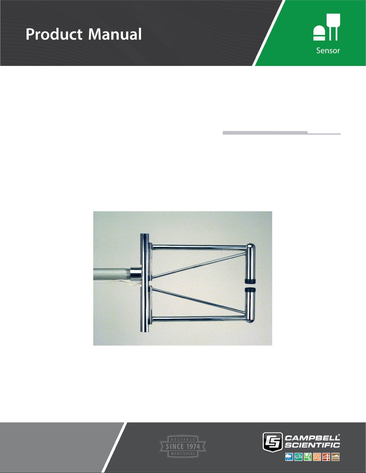
Krypton Hygrometer

05/2020

2010 – 2020

Page 2

PDF viewers: These page numbers refer to the printed version of this document. Use the PDF reader bookmarks tab for links to specific sections.

1. Introduction................................................................ 1

2. Precautions ................................................................ 1

3. Initial Inspection ........................................................ 1

3.1 Components .........................................................................................1

4. Overview .................................................................... 1

5. Specifications ............................................................ 2

5.1 Measurements ......................................................................................2

5.2 Electrical ..............................................................................................2

5.3 Physical ................................................................................................2

6. Installation ................................................................. 3

6.1 Siting ....................................................................................................3

6.2 Mounting ..............................................................................................3

6.2.1 Parts and Tools Needed for Mounting ..........................................3

6.2.2 Mounting the KH20 Sensor ..........................................................3

6.2.3 Mounting the Electronics Box ......................................................4

6.3 Wiring ..................................................................................................6

6.4 Data Logger Programming ...................................................................7

6.4.1 KH20 Calibration ..........................................................................7

7. Maintenance and Calibration .................................... 7

7.1 Visual Inspection ..................................................................................8

7.2 Testing the Source Tube .......................................................................8

7.3 Testing the Detector Tube ....................................................................8

7.4 Managing the Scaling of KH20 ............................................................8

7.5 Calibration ............................................................................................9

Appendices

Calibrating KH20 .................................................... A-1

A.1 Basic Measurement Theory ............................................................. A-1

A.2 Calibration of KH20 ........................................................................ A-1

B. Example Program .................................................. B-1

Page 3

Table of Contents

C. EasyFlux® DL CR6KH20 ........................................ C-1

C.1 Introduction ...................................................................................... C-1

C.2 Precautions ....................................................................................... C-2

C.3 Wiring .............................................................................................. C-2

C.3.1 Required Sensors ...................................................................... C-3

C.3.2 Optional Sensors ....................................................................... C-3

C.3.2.1 VOLT116 Module .......................................................... C-3

C.3.2.2 Barometer ....................................................................... C-4

C.3.2.3 Fine Wire Thermocouple ................................................ C-4

C.3.2.4 GPS Receiver ................................................................. C-5

C.3.2.5 Radiation Measurements Option 1 ................................. C-5

C.3.2.6 Radiation Measurements Option 2 ................................. C-6

C.2.3.7 Precipitation Gage .......................................................... C-8

C.2.3.8 Soil Temperature ............................................................ C-9

C.2.3.9 Soil Water Content ......................................................... C-9

C.3.2.10 Soil Heat Flux Plates .................................................... C-10

C.4 Operation ........................................................................................ C-12

C.4.1 Set Constants in CRBasic Editor and Load Program .............. C-12

C.4.2 Enter Site-Specific Variables with Data Logger Keypad or

LoggerNet ............................................................................ C-14

C.4.3 Data Retrieval ......................................................................... C-19

C.4.4 Output Tables .......................................................................... C-19

C.4.5 Program Sequence of Measurement and Corrections ............. C-36

C.5 References ...................................................................................... C-37

D. Equations and Algorithms of Water Vapor

Density and Water Flux in KH20 Eddy-

Covariance Systems ........................................... D-1

D.1 Fundamental Equation .................................................................... D-1

D.2 Working Equation ........................................................................... D-2

D.3 Eddy-Covariance Water Flux .......................................................... D-2

D.4 Frequency Response of KH20 ......................................................... D-3

D.5 References ....................................................................................... D-4

Figures

6-1. Mounting KH20 to a tripod. .................................................................4

6-2. Proper mounting position of the electronics box. .................................5

6-3. Attaching cables to the electronics box. ...............................................6

A-1. KH20 ln(mV) vs. Vapor Density .................................................... A-2

C-1. Example screen from CRBasic Editor showing user-defined

configuration constants ............................................................... C-13

C-2. Custom keypad menu; arrows indicate submenus .......................... C-14

Tables

6-1. Wire Color, Function, and Data Logger Connection............................6

6-2. KH20 Calibration Ranges ....................................................................7

A-1. Linear Regression Results for KH20 ln(mV) vs. Vapor Density .... A-2

A-2. Final Calibration Values for KH20 ................................................. A-3

C-1. Default Wiring for Required Sensors ............................................... C-3

C-2. Default Wiring for CS106 Barometer .............................................. C-4

C-3. Default Wiring for Fine Wire Thermocouple ................................... C-4

Page 4

C-4. Default Wiring for GPS Receiver .................................................... C-5

C-5. Default Wiring for Radiation Measurement Option 1 ...................... C-5

C-6. Default Wiring for Radiation Measurements Option 2 .................... C-6

C-7. A21REL-12 Wiring .......................................................................... C-8

C-8. CNF4 Wiring .................................................................................... C-8

C-9. Default Wiring for Precipitation Gage ............................................. C-9

C-10. Default Wiring for Soil Thermocouple Probes ................................ C-9

C-11. Default Wiring for Soil Water Content Probes .............................. C-10

C-12. Default Wiring for Non-Calibrating Soil Heat Flux Plates ............ C-10

C-13. Default Wiring for Soil Heat Flux Plates (Self Calibrating) .......... C-11

C-14. Station Variables with Descriptions ............................................... C-15

C-15. microSD Flash Card Fill Times with 10Hz Measurement Rate ..... C-19

C-16. Data Output Tables ........................................................................ C-20

C-17. Data Fields in the Time_Series Data Output Table ........................ C-21

C-18. Data Fields in the Diagnostic Output Table ................................... C-22

C-19. Data Fields in the Monitor_CSAT3B Output Table ....................... C-22

C-20. Data Fields in the Flux_AmeriFluxFormat Output Table .............. C-22

C-21. Data Fields in the Flux_CSFormat Data Output Table .................. C-25

C-22. Data Fields in the Flux_Notes Output Table .................................. C-29

CRBasic Example

B-1. CR3000 Program to Measure Water Vapor Fluctuations ................. B-1

Table of Contents

iii

Page 5

KH20 Krypton Hygrometer

1. Introduction

The KH20 is a highly sensitive hygrometer designed for measurement of rapid fluctuations in atmospheric water vapor, not absolute concentrations. It is typically used together with a CSAT3B in eddy-covariance systems.

2. Precautions

• READ AND UNDERSTAND the Safety section at the back of this

manual.

• Although the KH20 is rugged, it should be handled as precision scientific

instrument.

3. Initial Inspection

• Upon receipt of the KH20, inspect the packaging and contents for damage.

• The model number and cable length are printed on a label at the

3.1 Components

The KH20 sensor consist of a sensor head with 2 m (6 ft) cables and an electronics box. The following are also shipped with the KH20:

File damage claims with the shipping company.

connection end of the cable. Check this information against the shipping documents to ensure the correct product and cable length are received (see Section 3.1, Components

• KH20CBL-L25 Power/Signal cable with 8 m (25 ft) length. If a

longer cable is desired, order a KH20CBL-L replacement cable and specify the desired length after -L (for example KH20CBL-L50).

• 1/2 Unit Desiccant Bag

• Rain Shield

• Horizontal Mounting Boom (51 cm 20 mm DN (20-inch 3/4 IPS)

threaded aluminum pipe)

• 3/4 x 3/4 in. Nu-Rail Crossover Fitting

• 4 mm (5/32 in) Allen Wrench

(p. 1)).

4. Overview

The KH20 is a krypton hygrometer for measuring water vapor fluctuations in the air. The name KH20 (KH-twenty) was derived from KH2O (K-H the sensor has been known with this name since 1985. It is typically used with

O), and

Page 6

KH20 Krypton Hygrometer

NOTE

the CSAT3B 3-D sonic anemometer for measuring latent heat flux (LE), using eddy-covariance technique.

The KH20 sensor uses a krypton lamp that emits two absorption lines: major line at 123.58 nm and minor line at 116.49 nm. Both lines are absorbed by water vapor, and a small amount of the minor line is absorbed by oxygen. The KH20 is not suitable for absolute water vapor concentration measurements due to its signal offset drift.

The KH20 heads are sealed and will not suffer damage should they get wet. In addition, the electronics box and the connectors are housed inside a rain shield that protects them from moisture. The KH20 is suitable for long-term continuous outdoor applications.

The KH20 sensor is comprised of two main parts: the sensor head and the electronics box. The sensor head comes with cables that connect the sensor to the electronics, a power/signal cable, and mounting hardware.

Discussion on the principles and theory of measurement is included in Appendix A, Calibrating KH20 (p. A-1).

Features:

5. Specifications

5.1 Measurements

Calibration Range: 1.7 to 19.5 g/m3 (nominal) Frequency Response: 100 Hz Operating Temperature Range: –30 to 50 °C

5.2 Electrical

Supply Voltage: 10 V to 16 VDC Current Consumption: 20 mA max at 12 VDC Power Consumption: 0.24 Watts Output Signal Range: 0 to 5 VDC

• High frequency response suitable for eddy-covariance applications

• Well-suited for long-term, unattended applications

• Compatible with Campbell Scientific CRBasic data loggers: CR6,

CR3000, CR1000X, CR800 Series, CR1000, CR5000, and CR9000(X)

5.3 Physical

Dimensions

Sensor Head: 29 x 23 x 3 cm (11.5 x 9 x 1.25 in) Electronics Box: 19 x 13 x 5 cm (7.5 x 5 x 2 in) Rain Shield with Mount: 29 x 18 x 6.5 cm (11.5 x 7 x 2.5 in) Mounting Pipe: 50 cm (20 in) Carrying Case: 64 x 38 x 18 cm (25 x 15 x 7 in)

Page 7

6. Installation

6.1 Siting

6.2 Mounting

6.2.1 Parts and Tools Needed for Mounting

KH20 Krypton Hygrometer

Weight

Sensor Head: 1.61 kg (3.55 lb) Electronics Box: 0.6 kg (1.4 lb) Rain Shield with Mount: 2.2 kg (4.75 lb) Mounting Pipe with Nu-rail: 0.45 kg (1.0 lb) Carrying Case: 4.3 kg (9.45 lb) Shipping: 9.2 kg (20.15 lb)

When installing the KH20 sensor for latent heat flux measurement in an eddycovariance application, proper siting, sensor height, sensor orientation and fetch are important.

The following user-supplied hardware is required to mount the KH20 sensor:

1. Tripod (CM115 standard) or tower

2. Campbell Scientific crossarm (CM204 standard)

3. 3/4-inch IPS Aluminum Pipe, 12 inches long

4. 3/4-inch-by-1-inch Nu-Rail Crossover Fitting

5. Small Phillips and flat-head screwdrivers

6. 1/2-inch wrench

6.2.2 Mounting the KH20 Sensor

Mount the KH20 sensor head as follows:

1. Attach the 51 cm (20 in) mounting boom to the KH20.

2. Mount a crossarm to a tripod or tower.

3. Mount the 12-inch-long pipe to a crossarm via 1-inch-by-3/4-inch Nu-Rail

Crossover Fitting.

4. Mount the KH20 onto the 30 cm (12 in) pipe using a 3/4-inch-by-3/4-inch

Nu-Rail Crossover Fitting. Mount the KH20 such that the source tube, the longer of the two tubes, is positioned on top, as shown in FIGURE 6-1. Use cable ties to secure loose cables to the tripod or tower mast.

Page 8

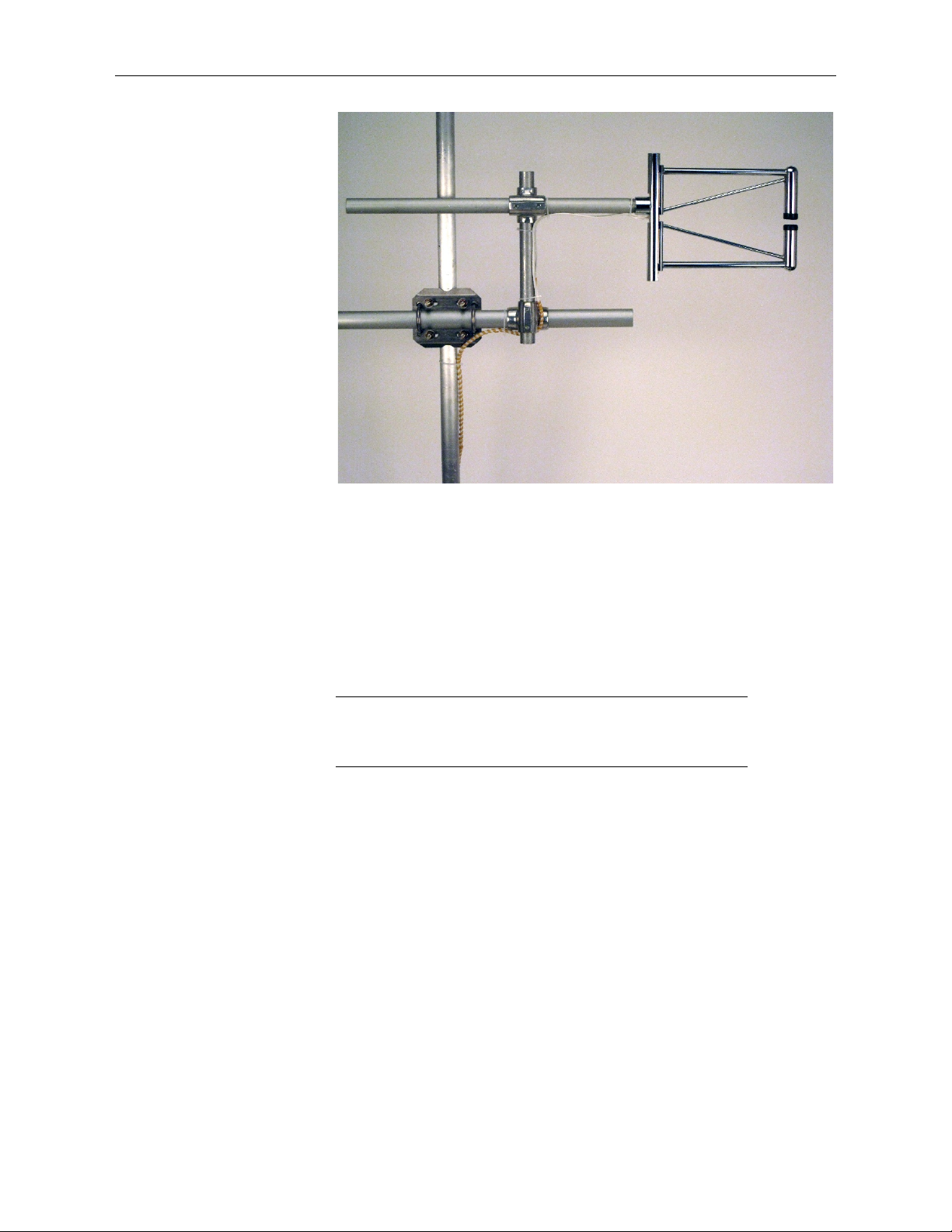
FIGURE 6-1. Mounting KH20 to a tripod.

NOTE

KH20 Krypton Hygrometer

6.2.3 Mounting the Electronics Box

Mount the electronics box as follows:

1. Remove the front cover of the rain shield by loosening the two pan-head

screws on the bottom front of the rain shield, and then pushing the cover all the way up, and sliding it out.

It will be difficult to mount the rain shield to a mast with the front cover on, since the 1/2-inch nut holding the bottom U-bolt is located inside the rain shield.

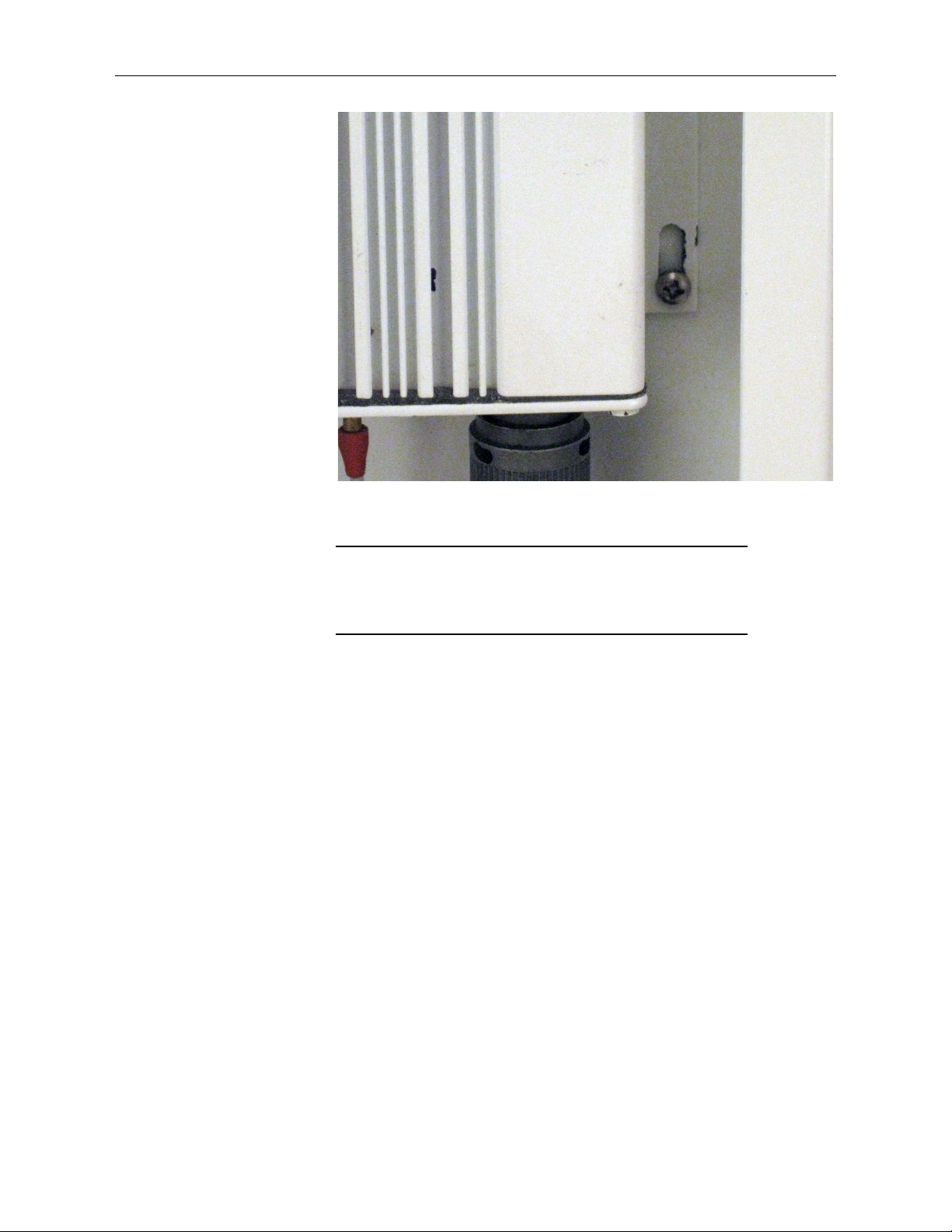
2. Before mounting the rain shield to a tripod, first mount the electronics box

inside the rain shield. Remove the four pan-head screws from the back panel of the rain shield. Align the electronics box and use the four panhead screws to secure the electronics box onto the back panel. Make sure the electronics box is pushed all the way up, and the screws are positioned at the bottom of the mounting slot on the electronics box (see FIGURE

6-2). This will provide enough room to attach the connectors to the bottom

of the electronics box later.

Page 9

KH20 Krypton Hygrometer

NOTE

FIGURE 6-2. Proper mounting position of the electronics box.

If the electronics box is not pushed all the way up during mounting, you will not have enough room to attach the connectors to the bottom of the electronics box, as the U-bolt for the rain shield will block the position of the connectors.

3. Mount the rain shield onto the tripod or tower mast using the U-bolt

provided. Make sure that the distance between the KH20 sensor head and the rain shield is within 5 feet so that the cables from the sensor head will be within reach of the electronics box. Also make sure that the rain shield is mounted vertically with an opening pointing downward so that the rain will effectively run down the rain shield and not penetrate inside.

Page 10

KH20 Krypton Hygrometer

TABLE 6-1. Wire Color, Function, and Data Logger Connection

⏚

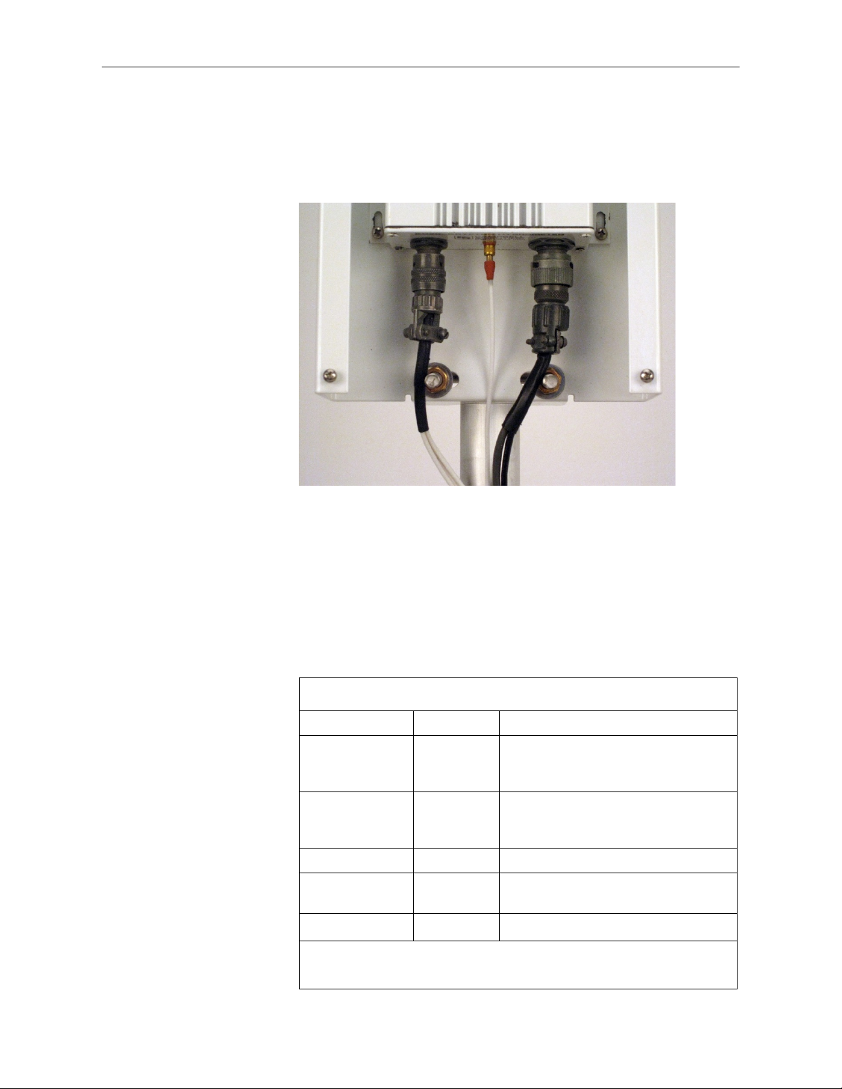
4. Connect the three cables to the bottom of the electronics box around the

U-bolt on the rain shield (see FIGURE 6-3). If there is not enough room for the connectors around the U-bolt, make sure the electronics box is mounted at a highest possible position (see step 2).

6.3 Wiring

FIGURE 6-3. Attaching cables to the electronics box.

5. Place the front cover back on the rain shield and tighten the two pan-head

screws to secure it in place.

6. Gather any loose cables and tie them up, using cable ties, onto the tripod or

tower mast.

Wire Wire Label Data Logger Connection Terminal

1, 2

White Signal

Black (from

white/black set)

Signal

Reference

U configured for differential input

DIFF H (differential high, analog-

voltage input)

U configured for differential input

DIFF L (differential low, analog-

voltage input)

Red Power 12V 12V

Black (from

red/black set)

Clear Shield

U terminals are automatically configured by the measurement instruction.

Jumper to ⏚ with a user-supplied wire.

Power

Ground

(analog ground)

Page 11

6.4 Data Logger Programming

TABLE 6-2. KH20 Calibration Ranges

The KH20 sensor outputs 0 to 5 VDC analog signal. These signals can be measured using the VoltDiff instruction on the CRBasic data loggers.

Programming basics for CRBasic data loggers are in the following sections. Complete program examples for select CRBasic data loggers can be found in Appendix B, Example Program

6.4.1 KH20 Calibration

Each KH20 is calibrated over a vapor range of approximately 2 to 19 g/m3. The calibration is performed twice under the following two conditions: window clean, and scaled. The water vapor absorption coefficient for three different vapor ranges are calculated from the collected calibration data: full range, dry range, and wet range. TABLE 6-2 shows a sample of the KH20 vapor ranges over which three different water vapor absorption coefficients are calculated. See Appendix A, Calibrating KH20 calibration.

KH20 Krypton Hygrometer

(p. B-1).

(p. A-1), for more information on KH20

Ranges Vapor Density (g/m3)

Full Vapor Range 2 – 19

Dry Vapor Range 2 – 9.5

Wet Vapor Range 8.25 – 19

Before the water vapor absorption coefficient, k logger program for the KH20, the following decisions must be made:

• Will the windows be allowed to scale?

• What vapor range is appropriate for the site?

Once the decision is made, the appropriate k calibrations sheet. The calibration sheet also contains the path length, x, for a specific KH20. Using the water vapor absorption coefficient for either the dry or the wet vapor range will produce more accurate measurements than using that for the full range. If the vapor range of the site is unknown, or if the vapor range is on the border line between the dry and the wet vapor ranges, the full range should be used.

7. Maintenance and Calibration

The KH20 sensor is designed for continuous field application and requires little maintenance. The tube ends for the KH20 have been sealed with silicone elastomer using an injection-mold method. Therefore, the tubes are protected from water damage, and the KH20 continues to make measurements under rainy or wet conditions. If the water tends to pool up on the tube window and blocks the signal, turn the sensor head at an angle so as to shed the water off the tube window. The rain shield protects the electronics box and the connectors from moisture.

, is entered into the data

can be chosen from the

Page 12

7.1 Visual Inspection

NOTE

• Make sure the optical windows are clean.

• Inspect the cables and connectors for any damage or corrosion. If you see

a discoloration on the white co-axial cable, you may suspect that the cable has water damage.

7.2 Testing the Source Tube

The source tube is the longer of the two tubes. Check to see if the source tube is working properly by performing the following test.

First, make sure the UV light is emitted from the source tube. To do this, you may look into the source tube (the longer of the two tubes), and you should see a bright blue light emitted from it.

Avoid looking into the source tube for an extended period of time when the KH20 is powered on to minimize the prolonged exposure to the UV light.

KH20 Krypton Hygrometer

If you see a faint or flickering blue light, perform the following test.

Check the current drain on the KH20

Typical current drain for the KH20 during normal operation should be 15 ~ 20 mA. The current drain of around 5 mA or less indicates the problem on the source tube. Obtain an RMA from Campbell Scientific and send the unit in for repair.

Check the voltage signal output from the KH20

If the voltage output reading is below 50 mV, you may have problems with either the source tube or the detector tube (Section 7.3, Testing the Detector Tube

(p. 8)).

7.3 Testing the Detector Tube

If the source tube tests fine but the output from KH20 is still in question, perform the following test. Prepare a piece of paper and insert it between the source tube and the detector tube to completely block the optical path. You should see an immediate decrease in the voltage reading, and it should go close to zero. No noticeable change in the voltage output, when the optical path is completely blocked, indicates a problem in the detector tube. If the decrease in the voltage reading takes place but the reading remains below 50 mV, when the paper is removed from the optical path, the source tube may be at fault. Obtain an RMA from Campbell Scientific and send the unit in for repair.

7.4 Managing the Scaling of KH20

The KH20 cannot be used to measure an absolute concentration of water vapor, because of scaling on the source tube windows caused by disassociation of atmospheric continuants by the ultra violet photons (Campbell and Tanner,

Page 13

KH20 Krypton Hygrometer

NOTE

1985 and Buck, 1976). The rate of scaling is a function of the atmospheric humidity. In a high humidity environment, scaling can occur within a few hours. That scaling attenuates the signal and can cause shifts in the calibration curve. However, the scaling over a typical flux averaging period is small. Thus, water vapor fluctuation measurements can still be made with the hygrometer.

To see if the source tube window has been scaled, get a clean, dry cotton swab and slide it across the source tube window. The scale is not visible to the naked eye, but if the window is scaled, you will feel a slight but noticeable resistance while you slide the swab across the window. There will be little resistance if the window is not scaled. If you determine the window is scaled, you can clean it with a wet cotton swab.

Use distilled water and a clean cotton swab to clean the scaled window. After cleaning the window, slide a clean, dry swab across the window to confirm the scale has been removed.

You can use the water vapor absorption coefficient for scaled window from the calibration sheet if the window will be allowed to scale during measurements.

7.5 Calibration

For quality assurance of the measured data, Campbell Scientific recommends the KH20 be recalibrated every two years. Calibrations require a returned material authorization (RMA) and completion of the “Declaration of Hazardous Material and Decontamination” form. Refer to the Assistance page at the end of this manual for more information.

For more information on the calibration process, refer to Appendix A, Calibrating KH20

(p. A-1).

Page 14

−

)ln(ln

−

lnln VxkV

+−=

Appendix A. Calibrating KH20

A.1 Basic Measurement Theory

The KH20 uses an empirical relationship between the absorption of the light and the material through which the light travels. This relationship is known as the Beer’s law, the Beer-Lambert law, or the Lambert-Beer law. According to the Beer’s law, the log of the transmissivity is anti-proportional to the product of the absorption coefficient of the material, k, the distance the light travels, x, and the density of the absorbing material, ρ. The KH20 sensor uses the UV light emitted by the krypton lamp: major line at 123.58 nm and the minor line at 116.49. As the light travels through the air, both the major line and the minor line are absorbed by the water vapor present in the light path. This relationship can be rewritten as follows, where k vapor, x is the path length for the KH20 sensor, and ρ density.

A-1

is the absorption coefficient for water

is the water vapor

If we express the transmissivity, T, in terms of the light intensity before and after passing through the material as measured by the KH20 sensor, V and V respectively, we obtain the following equation.

Taking the natural log of both sides, and solving for the density, ρ following equation.

If the path length, x, and the absorption coefficient for water, k becomes possible to measure the water vapor density ρ signal output, V, from KH20.

A.2 Calibration of KH20

The KH20 calibration process is to find the absorption coefficient of water vapor, k

. To do this, we rewrite the equation A-3, and solve for ln(V).

A-2

, yields the

A-3

are known, it

, by measuring the

A-4

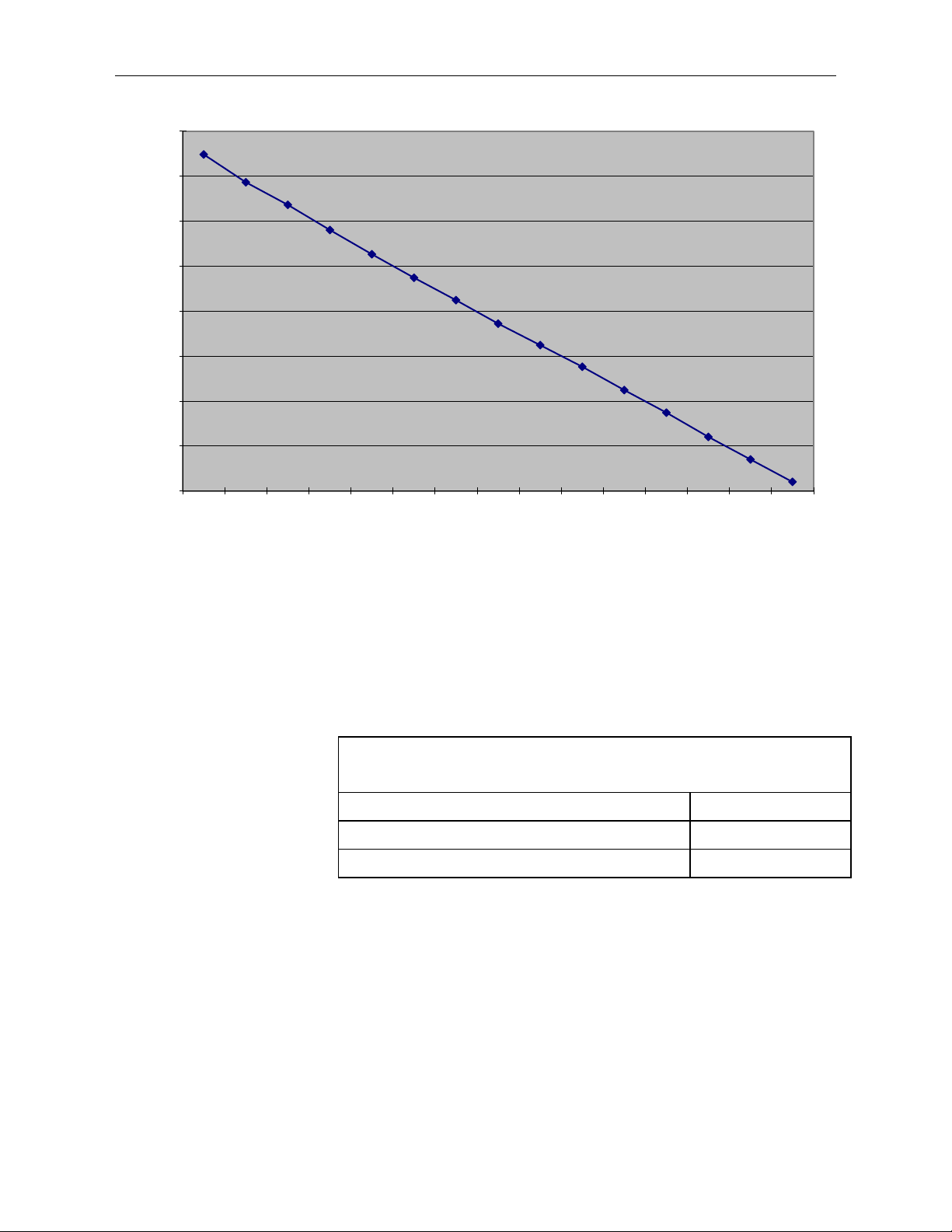
It now becomes obvious from the equation A-4 that there is a linear relationship between the natural log of the KH20 measurement output, lnV, and the water vapor density, ρ after we ran a KH20 over a full calibration vapor range.

. FIGURE A-1 shows the plot of the equation A-4

A-1

Page 15

Appendix A. Calibrating KH20

TABLE A-1. Linear Regression Results for KH20 ln(mV)

KH2O Output (mV)

Vapor Density (g/m3)

7.5

6.5

5.5

4.5

1.74 3.02 4.17 5.44 6.71 7.95 9.2 10.47 11.69 12.9 14.22 15.46 16.78 18.04 19.25

FIGURE A-1. KH20 ln(mV) vs. Vapor Density

We can perform the linear regression on the plot to obtain the slope for the relationship between the ln(mV) and the vapor density. The slope for the graph is the coefficient, k

x. TABLE A-1 shows the result of linear regression

analysis. The slope is the product of the absorption coefficient of water vapor,

, and the KH20 path length, x.

vs. Vapor Density

Description Values

Slope (xkw) –0.205

Y Intercept (ln(V0) 8.033

If we substitute these values, along with the measured lnV into equation A-3, we can obtain the water vapor density, ρ

. Campbell Scientific performs the

calibration twice for each KH20: once with the window cleaned, and again with the window scaled. We then break up the vapor density range into dry and wet ranges, and compute the k range. If you know the vapor density range for your site, it is recommended that you select the coefficient, k

values for each sub range, as well as for the full

, that is appropriate for your site, the dry range

or the wet range. If the vapor range for the site is unknown, or if the vapor range is on the border line between the dry and the wet ranges, use the value for the full range. TABLE A-2 shows the final calibration values the KH20 calibration certificate contains. The data shown in TABLE A-2 is from an actual KH20.

A-2

Page 16

Appendix A. Calibrating KH20

TABLE A-2. Final Calibration Values for KH20

Vapor Range

)

(g/m

Slope (xkw)

Y Intercept

ln (V0)

Coefficient

(kw)

Full Range 1.74 ~ 19.25 -0.205 3087 -0.144

Dry Range 1.74 ~ 9.20 -0.216 3259 -0.151

Wet Range 7.95 ~ 19.25 -0.201 2899 -0.141

A-3

Page 17

Appendix B. Example Program

CRBasic Example B-1. CR3000 Program to Measure Water Vapor Fluctuations

'CR3000 Series Data Logger

Units kh_mV = mV

NOTE

'This data logger program measures KH20 Krypton Hygrometer.

'The station operator must enter the constant and the calibration value for the KH20. 'Search for the text string "unique" to find the locations of these constants 'and enter the appropriate values found from the calibration sheet of the KH20.

'*** Unit Definitions ***

'Units Description 'ln_mV ln(mV) (natural log of the KH20 millivolts) 'mV millivolts 'rho_w g/m^3

'*** Wiring ***

'ANALOG INPUT '1H KH20 signal+ (white) '1L KH20 signal- (black) 'gnd KH20 shield (clear)

'EXTERNAL POWER SUPPLY 'POS KH20 power+ (red) ' data logger POWER IN 12 (red) 'NEG KH20 power- (black) ' KH20 power shield (clear) ' data logger POWER IN G (black)

PipeLineMode

'*** Constants ***

'Measurement Rate '10 Hz

Const SCAN_INTERVAL = 100 '100 mSec

'Output period

Const OUTPUT_INTERVAL = 30 'Online flux data output interval in minutes. Const x = 1 'Unique path length of the KH20 [cm]. Const kw = -0.150 'Unique water vapor absorption coefficient [m^3 / (g cm)]. Const xkw = x*kw 'Path length times water vapor absorption coefficient [m^3 / g].

'*** Variables ***

Public panel_temp Public batt_volt Public kh(2) Public rho_w Alias kh(1) = kh_mV Alias kh (2) = ln_kh Units panel_temp = deg_C Units batt_volt = volts

The following example program measures the KH20 at 10Hz, and stores the average values into a data table called ‘stats’, as well as the raw data into a data table called ‘ts_data’.

The KH20 does not monitor absolute water vapor concentration.

B-1

Page 18

Units ln_kh = ln_mV

EndProg

Appendix B. Example Program

Units rho_w = g/m^3

'*** Data Output Tables *** 'Processed data

DataTable (stats,True,-1)

DataInterval (0,OUTPUT_INTERVAL,Min,10) Minimum (1,batt_volt,FP2,False,False) Average (1,panel_temp,FP2,False) Average (2,kh(1),IEEE4,False)

EndTable

'Raw time-series data.

DataTable (ts_data,True,-1)

DataInterval (0,SCAN_INTERVAL,mSec,100) Sample (1,kh_mV,IEEE4)

EndTable

'*** Program ***

BeginProg

Scan (SCAN_INTERVAL,mSec,3,0)

'data logger panel temperature. PanelTemp (panel_temp,250)

'Measure battery voltage. Battery (batt_volt)

'Measure KH20. VoltDiff (kh_mV,1,mV5000,1,TRUE,200,250,1,0) ln_kh = LOG(kh_mV) rho_w = ln_kh/xkw

CallTable stats CallTable ts_data

NextScan

B-2

Page 19

NOTE

EasyFlux is

Appendix C. EasyFlux® DL CR6KH20

C.1 Introduction

EasyFlux® DL CR6KH20 is a CRBasic program that enables a CR6 data logger, along with a KH20 and CSAT3B, to collect fully corrected fluxes of latent heat (H EC data using commonly used corrections in the scientific literature. The program can also calculate the ground surface heat flux and energy closure by adding an optional suite of energy balance sensors. Because the energy balance sensors require more analog terminals than the CR6 has, the program supports the addition of a VOLT116 (or CDM-A116) analog terminal expansion module.

Specifically, the program supports data collection and processing from the following sensors.

REQUIRED SENSORS:

KH20 Krypton Hygrometer (qty 1) CSAT3B Sonic Anemometer (qty 1) Temperature/Relative Humidity (RH) Probe (qty 1). Supported Models:

OPTIONAL SENSORS:

CS106 Barometer (qty 0 to 1) FW3 Fine Wire Thermocouple (qty 0 to 1) GPS16X-HVS GPS Receiver (qty 0 to 1) Radiation measurements

TE525MM Rain Gage (qty 0 to 1) TCAV Soil Thermocouple Probe (qty 0 to 3) Soil Water Content Reflectometer (qty 0 to 3)

Soil Heat Flux Plates

O), sensible heat, and momentum. The program processes the

o HMP155A o EE181

o Option 1

− NR-LITE2 Net Radiometer (qty 0 to 1)

− CS301 or CS320 Pyranometer (qty 0 to 1)

− CS310 Quantum Sensor (qty 0 to 1)

− SI-111 Infrared Radiometer (qty 0 to 1)

o Option 2

− SN500SS, or NR01, or CNR4 4-Way Radiometer

(qty 0 to 1; if using CNR4, the CNF4 Ventilation and Heating Unit is also supported)

o CS650 o CS655

o Option 1: HFP01 plates (qty 0 to 3) o Option 2: HFP01SC self-calibrating plates (qty 0 to 3)

It may be possible to customize the program for other sensors or quantities in configurations not described here. Contact Campbell Scientific for more information.

a registered trademark of Campbell Scientific, Inc.

C-1

Page 20

C.2 Precautions

NOTE

Appendix C. EasyFlux® DL CR6KH20

The VOLT116 and CDM-A116 are functionally the same, however their OSes are not interchangeable. If updating an OS, make sure it is for the correct model.

EasyFlux DL CR6KH20 requires the CR6 to have operating system (OS)

version 09.02 or newer. If using a VOLT116, it must have OS v.01 or newer, or if using a CDM-A116, it must have v.06 or newer.

The program applies the most common EC corrections to fluxes. However, the

user should determine the appropriateness of the corrections for their site.

Campbell Scientific always recommends saving time-series data in the event

reprocessing of raw data is warranted. Further, the user should determine the quality and fitness of all data for publication, regardless of whether said data were processed by EasyFlux DL CR6KH20 or another tool.

As EasyFlux DL CR6KH20 is not encrypted, users have the ability to view and

edit the code. However, Campbell Scientific does not guarantee the function of an altered program.

C.3 Wiring

When wiring the sensors to the data logger or VOLT116, the default wiring schemes, along with the number of instruments EasyFlux DL CRKH20 supports, should be followed if the standard version of the program is being used. TABLE C-1 through TABLE C-13 present the wiring schemes.

A KH20 and CSAT3B are the only required sensors for the program. The additional sensors described in the following tables are optional, although the CS106 and FW3 are recommended. Many of the optional sensors are wired to a VOLT116 (or CDM-A116) module, which effectively increases the CR6 analog terminals. If one or more of the optional sensors are not used, the data logger or VOLT116 terminals assigned to those sensor wires should be left unwired.

If the standard data logger program is modified, the wiring presented in TABLE C-1 may no longer apply. In these cases, refer directly to the program code to determine proper wiring.

If using an analog expansion module, all wiring and connections are the same whether using a VOLT116 or a CDM-A116. Therefore, throughout this appendix, the wiring terminals are only listed for the VOLT116.

C-2

Page 21

Appendix C. EasyFlux® DL CR6KH20

TABLE C-1. Default Wiring for Required Sensors

⏚

⏚.

C.3.1 Required Sensors

A KH20, CSAT3B, and Temp/RH Probe must be wired to the CR6 for EasyFlux DL CR6KH20 to be functional. TABLE C-1 shows the default wiring for these sensors.

Sensor Quantity Wire Description Color Terminal

Signal White U3

Signal Reference Black U41/

KH20 1

CSAT3B 1

Power Cable, Ground

HMP155A/EE1812/

Temp/RH Probe

Wire a user-supplied jumper from U4 to

Wire colors for the HMP155A are shown in normal font, while colors for the EE181 are italicized.

Due to terminal constraints, the Temp/RH Probe is a single-ended (SE) voltage measurement. As an SE measurement from a sensor that is powered continuously, wire the signal reference and power ground wires both to G.

Power Red 12V

Power Ground Black G (power ground)

Shield Clear

CSAT3BCBL3 CPI

Cable

CSAT3BCBL2

Power Cable, 12V

CSAT3BCBL2

RJ45 Connector

Red 12V

Black G

(analog ground)

CR6 CPI Port (if no

Volt116) or

Volt116 CPI Port

Temp Signal Yellow/Yellow U5

RH Signal Blue/Blue U6

RH Signal Reference White/Black

Shield Clear/Clear

Power Red/Red +12 V

Power Ground Black/None G3/

C.3.2 Optional Sensors

C.3.2.1 VOLT116 Module

Due to the limitations on terminal count of the CR6, a VOLT116 (or CDM-A116) module is required when adding optional sensors. Prepare the module as follows:

1. Connect the module to a 10-32 VDC power source.

2. Launch Campbell Scientific Device Configuration Utility software (v2.12

or newer) and select VOLT116. If this is the first time connecting, follow the instructions on the main screen to download and install the USB driver to the computer.

3. Select the appropriate COM port and click Connect.

C-3

Page 22

Appendix C. EasyFlux® DL CR6KH20

TABLE C-2. Default Wiring for CS106 Barometer

⏚

TABLE C-3. Default Wiring for Fine Wire Thermocouple

⏚

4. Once connected, a list of settings is shown. Navigate to CPI Address and

change the value to 1. Press Apply and exit the software.

5. Use an Ethernet cable (included with the module) to connect the module

CPI port to the CR6 CPI port.

C.3.2.2 Barometer

A CS106 Barometer is recommended for increased accuracy due to calculations and unit conversions that use ambient pressure. TABLE C-2 shows the default wiring for EasyFlux DL CR6KH20.

Sensor Quantity Wire Description Color CR6 Terminal

Signal Blue U7

Signal Reference Yellow

CS106 Barometer 0 or 1

Shield Clear

12V Red 12V

Power Ground Black G

Trigger (not used) Green G

C.3.2.3 Fine Wire Thermocouple

A fine wire thermocouple is recommended for a more accurate and direct measurement of sensible heat flux. If no fine wire thermocouple is used, an estimate of sensible heat flux is still given; it is derived using the covariance of sonic temperature and vertical wind and applying the SND correction. The EasyFlux DL CR6KH20 can support from zero to one fine-wire thermocouple. Shown in TABLE C-3 are the available types and default wiring for adding a fine-wire thermocouple.

VOLT116

Sensor Quantity Wire Description Color

Signal

FW3 Fine Wire

Thermocouple

The FW05 and FW1 may be used instead of the FW3, although they are more fragile and may require more

frequent replacement.

0 or 1

Signal Reference

Shield Clear

Purple

Red

Terminal

Diff 15H

Diff15L

C-4

Page 23

Appendix C. EasyFlux® DL CR6KH20

TABLE C-4. Default Wiring for GPS Receiver

⏚

TABLE C-5. Default Wiring for Radiation Measurement Option 1

Signal

White

CR6 U11

⏚

C.3.2.4 GPS Receiver

A GPS receiver such as the GPS16X-HVS is optional, but will keep the data logger clock synchronized to GPS time. If the CR6 clock differs by one millisecond or more, EasyFlux DL CR6OP will resynchronize the data-logger clock to match the GPS. The GPS receiver also calculates solar position. TABLE C-4 shows the default wiring for the GPS16X-HVS.

Sensor Quantity Wire Description Color CR6 Terminal

PPS Grey U1

TXD White U2

Shield Clear

GPS16X-HVS 0 or 1

12V Red 12V

Power Ground Black G

Unused Yellow and Blue G

C.3.2.5 Radiation Measurements Option 1

There are two options for making radiation measurements with EasyFlux DL CR6KH20 . The program can support a combination of the sensors described in TABLE C-5. Alternatively, it can support one of the three types of four-way radiometers described in TABLE C-6. TABLE C-5 gives the default wiring for Option 1. TABLE C-6 shows the details of the default wiring for Option 2.

Sensor Quantity Wire Description Color

Radiation Signal Red CR6 U8

NR-LITE2 Net

Radiometer

CS301

Pyranometer

0 or 1

Signal Reference Blue

Shield Black

Signal White VOLT116 Diff 9H

Signal Reference Black VOLT116 Diff 9L2/

Shield Clear

Signal Reference Blue

CS320 Digital

Pyranometer

0 or 1

Shield Clear

12V Power Red CR6 12V

Terminal

CR6 ⏚

VOLT116 ⏚

CR6

Power Ground Black CR6 G

Signal Red

CS310

Quantum Sensor

0 or 1

Signal Reference Black VOLT116 Diff 10L

Shield Clear

VOLT116 Diff

10H

VOLT116 ⏚

C-5

Page 24

Appendix C. EasyFlux® DL CR6KH20

TABLE C-5. Default Wiring for Radiation Measurement Option 1

TABLE C-6. Default Wiring for Radiation Measurements Option 2

⏚

Sensor Quantity Wire Description Color

Target Temp Signal Red/White

Terminal

VOLT116 Diff

11H

Target Temp Reference Black/Black VOLT116 Diff 11L

SI-111/SI-111SS

Infrared

Radiometer

0 or 1

Sensor Temp Reference Blue/Blue

Shield Clear/Clear

Sensor Temp Signal Green/Green

VOLT116 ⏚

VOLT116 Diff

12H

VOLT116 ⏚

Voltage Excitation White/Red VOLT116 X3

Use only one pyranometer, the CS301 or the CS320. Use the CS320 for applications where a digital, optionally-heated sensor is preferred.

Jumper to ⏚ with user-supplied wire

C.3.2.6 Radiation Measurements Option 2

Three models of four-way radiometers are compatible with EasyFlux DL CR6KH20, however only one may be used at a given time. The default wiring for each of the four-way radiometers is shown in TABLE C-6.

Sensor Quantity Wire Description Color Terminal

SN500SS 4-Way

Radiometer

NR01 4-Way

Radiometer

0 or 1

SDI-12 Signal White CR6 U11

Shield Clear

CR6

Power Red CR6 12V

Power Ground Black G

Pyranometer Up Signal Red (cbl 1) VOLT116 Diff 9H

Pyranometer Up Reference Blue

(cbl 1)

Pyranometer Down Signal White (cbl 1)

Pyranometer Down

Reference

Green

(cbl 1)

Pyrgeometer Up Signal Brown (cbl 1)

Pyrgeometer Up Reference

Yellow

(cbl

Pyrgeometer Down Signal Purple (cbl 1)

Pyrgeometer Down

Reference

Grey

(cbl 1)

PT100 Signal White (cbl 2) VOLT116 Diff 4H

PT100 Reference Green (cbl 2) VOLT116 Diff 4L

VOLT116 Diff

10H

VOLT116 Diff

10L

VOLT116 Diff

11H

VOLT116 Diff

11L

VOLT116 Diff

12H

VOLT116 Diff

12L

C-6

Page 25

Appendix C. EasyFlux® DL CR6KH20

TABLE C-6. Default Wiring for Radiation Measurements Option 2

Sensor

Quantity

Wire Description

Color

Terminal

⏚

VOLT116 Diff

⏚

Current Excite Red (cbl 2) VOLT116 X1

Current Return Blue (cbl 2)

VOLT116 ⏚

CNR4 4-Way

Radiometer

Jumper to ⏚ with user-supplied wire

Shields Clear

VOLT116

Pyranometer Up Signal Red VOLT116 Diff 9H

VOLT116 Diff

10H

VOLT116 Diff

10L

VOLT116 Diff

11H

11L1/

VOLT116 Diff

12H

VOLT116 Diff

12L

0 or 1

Pyranometer Up Reference Blue1/

Pyranometer Down Signal White

Pyranometer Down

Reference

Black

Pyrgeometer Up Signal Grey

Pyrgeometer Up Reference Yellow1/

Pyrgeometer Down Signal Brown

Pyrgeometer Down

Reference

Green

Thermistor Signal White VOLT116 Diff 4H

Thermistor V Excite Red VOLT116 X1

Thermistor Reference Black

Shields Clear

VOLT116

A CNF4 Ventilation and Heater Unit may be used with the CNR4 4-way Radiometer for more accurate radiation measurements. The CNF4 requires a solid state relay to control the ventilator and heater. The A21REL-12 4-Channel Relay Driver, sold separately, is recommended. Install the A21REL12 inside the system enclosure near the VOLT116 and data logger. TABLE

C-7 lists the wiring connections needed to power and control the A21REL-12;

a CABLE3CBL-1 or similar 3-conductor 22 AWG cable is recommended for connections from the A21REL-12 to the VOLT116, and a CABLEPCBL-1 or similar 16 AWG 2-conductor power cable is recommended for power connections from the A21REL-12 to system 12V power source. TABLE C-8 lists the wiring for the CNF4.

C-7

Page 26

Appendix C. EasyFlux® DL CR6KH20

A21REL-12 Terminal

Connecting Terminal

Cable/Wire

CABLEPCBL-1,

CABLE3CBL-1,

TABLE C-8. CNF4 Wiring

Sensor

Quantity

Wire Description

Color

Terminal

A21REL-12

TABLE C-7. A21REL-12 Wiring

+12V

System +12V

Ground System GND1/

CTRL 1

CTRL 2

CTRL 3

The +12V terminal on the A21REL-12 needs to be in common with the REL 1 COM, REL 2 COM, and REL 3 COM terminals. To do this, use jumper wires to connect the +12V terminal to REL 1 COM, and then REL1 COM to REL 2 COM, and finally REL2 Com to REL 3 COM.

For the A21REL-12 power connections, connect +12V and G to a system or external

power supply. Do not connect to the +12V or G terminals on the CR6 or VOLT116.

VOLT116 SW5V #1

VOLT116 SW5V #2

VOLT116 SW5V #3

CABLEPCBL-1,

red wire

black wire

CABLE3CBL-1,

red wire

black wire

CABLE3CBL-1,

white wire

Tachometer Output Green CR6 U11

CNF4

0 or 1,

only use

with a

CNR4

Tachometer

Reference

Ventilator Power Yellow

Ventilator Ground Brown

Heater #1 Power White

Grey

A21REL-12

REL 1 NO

A21REL-12

REL 2 NO

CR6 ⏚

REL G

Heater #1 Ground Red

Heater #2 Power Black

Heater #2 Ground Blue

C.2.3.7 Precipitation Gage

EasyFlux DL CR6KH20 can support a single TE525MM tipping rain gage. The default wiring for the precipitation gage is shown in TABLE C-9.

REL G

A21REL-12

REL 3 NO

A21REL-12

REL G

C-8

Page 27

Appendix C. EasyFlux® DL CR6KH20

TABLE C-9. Default Wiring for Precipitation Gage

⏚

TABLE C-10. Default Wiring for Soil Thermocouple Probes

VOLT116 Terminal

⏚

CAUTION

NOTE

Sensor Quantity Wire Description Color

TE525MM

Tipping Rain

Gage

0 or 1

Pulse Output Black U12

Signal Ground White

Shield Clear

C.2.3.8 Soil Temperature

The TCAV is an averaging soil thermocouple probe used for measuring soil temperature. EasyFlux DL CR6KH20 can support up to three TCAV probes. The order of wiring, however, is important. If only one TCAV sensor is used, it must be wired as described for TCAV #1 in TABLE C-10. A second or third TCAV sensor would be wired according to TCAV #2 or TCAV #3, respectively, in TABLE C-10.

If only one TCAV is being used and it is wired according to TCAV #2 or #3, the data logger will not record any TCAV measurements.

Sensor Quantity Wire Description Color

Signal Purple Diff 1H

TCAV #1 1

TCAV #2 1

Signal Reference Red Diff 1L

Shield Clear

Signal Purple Diff 2H

Signal Reference Red Diff 2L

Shield Clear

CR6 Terminal

Signal Purple

TCAV#3

Signal Reference Red

Shield Clear

The CS650 or CS655 sensors also measure soil temperature. If the CS650 or CS655 sensors are used but no TCAV probes are used, EasyFlux DL CR6KH20 will use soil temperature from the CS650 or CS655 to compute ground-surface heat flux. If available, soil temperature from the TCAV probe is preferred since it provides a better spatial average. See wiring details for these sensors in TABLE C-11.

C.2.3.9 Soil Water Content

EasyFlux DL CR6KH20 supports one of two models of soil water content sensors: the CS650 or CS655; up to three of one model is supported. A soil

Diff 3H

Diff 3L

C-9

Page 28

TABLE C-11. Default Wiring for Soil Water Content Probes

Sensor

Quantity

Wire Description

Color

CR6 Terminal

CS650/CS655

⏚

TABLE C-12. Default Wiring for Non-Calibrating Soil Heat Flux Plates

⏚

CAUTION

SDI-12 address 1

CS650/CS655

SDI-12 address 2

CS650/CS655

SDI-12 address 3

Appendix C. EasyFlux® DL CR6KH20

water content sensor can also be omitted without affecting function. The default wiring for each is shown in TABLE C-11.

If only one soil water content sensor is being used, wire it according to the first probe as described in TABLE C-11. If only one sensor is being used and it is wired according to the second or third sensor, EasyFlux DL CR6KH20 will not record any measurements from the soil water content sensor.

SDI-12 Data Green U9

SDI-12 Power Red +12 V

SDI-12 Reference Black G

Shield Clear G

Not Used Orange

SDI-12 Data Green U9

SDI-12 Power Red +12 V

SDI-12 Reference Black G

Shield Clear

Not Used Orange G

SDI-12 Data

SDI-12 Power

SDI-12 Reference

Shield Clear

Not Used

Green

Red

Black

Orange

+12 V

C.3.2.10 Soil Heat Flux Plates

EasyFlux DL CR6KH20 can support from zero to soil heat flux plates. The user has the option to use one of two supported models: the HFP01 or HFP01SC (self-calibrating). The default wiring for the HFP01 soil heat flux plates is shown in TABLE C-12, and the default wiring for the HFP01SC plates is shown in TABLE C-13.

Sensor Quantity Wire Description Color VOLT116 Terminal

Signal White Diff 5H

HFP01 #1 1

Signal Reference Green Diff 5L

Shield Clear

C-10

Page 29

Appendix C. EasyFlux® DL CR6KH20

TABLE C-12. Default Wiring for Non-Calibrating Soil Heat Flux Plates

Sensor

Quantity

Wire Description

Color

VOLT116 Terminal

⏚

TABLE C-13. Default Wiring for Soil Heat Flux Plates (Self Calibrating)

Sensor

Quantity

Wire Description

Color

VOLT116 Terminal

⏚

Signal White Diff 6H

HFP01 #2 1

Signal Reference Green Diff 6L

Shield Clear

Signal White Diff 7H

HFP01 #3 1

Signal Reference Green Diff 7L

Shield Clear

Signal White Diff 5H

Signal Reference Green Diff 5L

HFP01SC #1 1

Shield Clear

Heater Signal Yellow Diff 13H

Heater Reference Purple Diff 13L

Shield Clear

Heater Power Red SW12-11/

Power Reference Black G

Signal White Diff 6H

Signal Reference Green Diff 6L

Shield Clear

Heater Signal Yellow Diff 14H

HFP01SC #2 1

Heater Reference Purple Diff 14L

Shield Clear

Heater Power Red SW12-11/

Power Reference Black G

Signal White Diff 7H

Signal Reference Green Diff 7L

Shield Clear

Heater Signal Yellow Diff 16H

HFP01SC #3 1

Heater Reference Purple Diff 16L

Shield Clear

Heater Power Red SW12-21/

Power Reference Black G

The SW12 terminals on the VOLT116 are limited to 200mA output. Accordingly, no more than two HFP01SC sensors may be connected to each terminal. Connect heater power wires from HFP01SC #1 and #2 to SW12-1, and connect heater wires from HFP01SC #3 to SW12-2.

C-11

Page 30

C.4 Operation

C.4.1 Set Constants in CRBasic Editor and Load Program

Appendix C. EasyFlux® DL CR6KH20

Operating EasyFlux DL CR6KH20 requires the user to enter or edit certain constants and input variables unique to the program or site. Constants are typically edited only once when first initializing the program, whereas sitespecific variables are edited upon initial deployment and periodically as site conditions change; for example, canopy height is a variable that may need to be adjusted throughout a growing season. Appendix C.4.1, Set Constants in CRBasic Editor and Load Program constants, and Appendix C.4.2, Enter Site-Specific Variables with Data Logger Keypad or LoggerNet

Before operating the station, the values for configuration constants should be verified in the program code using CRBasic Editor.

Open the program in CRBasic Editor. After the introductory comments at the top is a section titled “USER-DEFINED CONFIGURATION CONSTANTS” (see FIGURE C-1). Review the constants in this section and modify as needed. If having difficulty locating the correct lines of code, search the program for the word “unique”. This will locate all lines of code containing constants that need to be verified. Look for the text comments on the right side of each line of code for more explanation of the constant. Generally, the constants fall into four categories:

(p. C-14), provides details on setting variables.

(p. C-12), provides instructions on setting

1. Program Function Constants

These are constants that determine the timing of code execution, frequency of writing to output tables, memory allocation, etc. In most cases, the default constants for these values may be retained.

A program function constant worth mentioning is ONE_FULL_TABLE. If this is set to TRUE, all of the intermediate and auxiliary measurements will be included as data fields in the main FLUX_CSFormat output table, rather than being in a separate output table called FLUX_NOTES. For more information, see Appendix C.4.4, Output Tables

2. Sensor Selection Constants

All sensor selection constants begin with the prefix SENSOR. The value is set to TRUE in the constant table if the system includes the sensor. For example, if a system has a fine-wire thermocouple, the constant SENSOR_FW should be set to TRUE. When set to TRUE, the wiring in TABLE C-13 will apply to the sensor and the data from that sensor will be included in the data output tables.

If a sensor is not used, ensure the constant is set to FALSE.

3. Sensor Quantity Constants

The value for these constants indicates the number of each type of sensor in the system. For example, if three soil heat flux (SHF) plates were being used, the constant NMBR_SHF would be set to 3.

(p. C-19).

4. Sensor Calibration Constants

Some sensors have unique parameters for their measurement

C-12

Page 31

Appendix C. EasyFlux® DL CR6KH20

NOTE

equations; for example, multipliers and/or offsets for linear working equations that are used to convert their raw measurements into the values applicable in analysis. Typically, these parameter values are found on the calibration sheet from the sensor original manufacturer. For example, if an NR-LITE2 net radiometer is being used, a unique multiplier is set in the following line of code: Constant NRLITE_SENSITIVITY = 16. The comments in the code explain that the value entered is the sensor sensitivity provided in the NRLITE2 calibration sheet.

Constants relating to a particular sensor have been grouped together and have the sensor selection constant at the beginning, such that if the sensor selection constant is set to FALSE, the other constants for that sensor may be ignored. For example, the constants dealing with the SI-111SS Infrared Radiometer are grouped together with the SENSOR_SI111 constant at the top. If a SI-111SS is not being used, SENSOR_SI111 should be set to FALSE and the next five constants dealing with calibration coefficients will be ignored in the program.

After all constants are verified, save the program under a new or modified file name to keep track of different program versions. Finally, send the program to the CR6 using LoggerNet, PC400, or PC200W software.

FIGURE C-1. Example screen from CRBasic Editor showing user-

defined configuration constants

C-13

Page 32

Appendix C. EasyFlux® DL CR6KH20

System Control Site Var Settings >

Site Var Settings: Latitude Hemisph_NS Longitude

Hemisph_EW Altitude Meas height Surface Type > Canopy Height

d, 0 = auto z0, 0 = auto Sonic Azmth

KH20 Coord x KH20 Coord y FW Coord x

FW Coord y FW Dim GPS Height Bulk Density C_dry_soil HFP Depth

Planar Fit Alpha > Planar Fit Beta > Footprt Dist Intrst >

Surface Type: CROP GRASS FOREST SHRUB BARELAND WATER ICE

Planar Fit Alpha: ≤60 or ≥300 >60 & ≤170 >170 & <190 ≥190 & <300

Planar Fit Beta: ≤60 or ≥300 >60 & ≤170 >170 & <190 ≥190 & <300

Footprt Dist Intrst: ≤60 or ≥300 >60 & ≤170 >170 & <190 ≥190 & <300

C.4.2 Enter Site-Specific Variables with Data Logger Keypad or

LoggerNet

After the eddy-covariance station is installed and the data logger is running the program, connect a CR1000KD Keyboard Display to the CR6 CS-I/O port to view a custom menu of station-specific variables (FIGURE C-2). Use this menu to enter, view, and modify these variables. Use the up and down arrow buttons to navigate to different variables. Press Enter to select a variable or to set a new value after typing it. Press Esc to return to the previous menu.

FIGURE C-2 depicts the structure of the custom menu. Bypass the custom menu to interact directly with the data logger through the data logger default menus. To bypass the custom menus, select < System Menu >. If no CR1000KD is available, these same variables may be viewed and edited using the LoggerNet connect screen numeric display of variables from the Public table.

FIGURE C-2. Custom keypad menu; arrows indicate submenus

Before fluxes are processed correctly, the user must go through each of the station variables and set or confirm the assigned values. TABLE C-14 gives short descriptions of each station variable.

C-14

Page 33

Appendix C. EasyFlux® DL CR6KH20

TABLE C-14. Station Variables with Descriptions

The height of the center of the

Distance along the sonic x-axis

Station Variable Units Default Description

Latitude

Hemisph_NS none NORTH

Longitude

Hemisph_EW none WEST

Altitude m 1356 The site altitude altitude

decimal

degrees

decimal

degrees

41.766

111.855

The site latitude in degrees North or South.

The site latitudinal hemisphere. Options are NORTH or SOUTH.

The site longitude in degrees East or West.

The site longitudinal hemisphere. Options are EAST or WEST.

Name of variable in

Public Table (in

case no CR1000KD

available)

Latitude

hemisphere_NS 1 = North –1 = South

Longitude

hemisphere_EW 1 = East –1 = West

Meas Height m 2

Surf Type none GRASS

Canopy Height m 0.5

d m 0 (Auto)

Sonic Azmth

m 0 (Auto)

decimal

degrees

eddy-covariance sensor measurement volumes above ground.

Type of surface at the measurement site. Options are CROP, GRASS, FOREST, SHRUB, BARELAND, and WATER. This is used to estimate displacement height.

The average height of the canopy.

Displacement height. Set to zero (0) for program to auto-calculate. See the Aerodynamic Height appendix in the EasyFlux DL CR6OP manual for details.

Roughness length. Set to zero (0) for program to auto-calculate. See the Programmatic Approach appendix in the EasyFlux DL CR6OP manual for details.

The compass direction in which the sonic negative x-axis points (the compass direction in which the sonic head is pointing).

height_measurement

surface_type 1 = CROP 2 = GRASS 3 = FOREST 4 = SHRUBLAND 5 = BARELAND 6 = WATER 7 = ICE

height_canopy

displacement_user

roughness_user

sonic_azimuth

KH20 Coord x

m 0.15

between the sonic sampling volume and KH20 sampling volume.

separation_x_kh20

C-15

Page 34

Appendix C. EasyFlux® DL CR6KH20

TABLE C-14. Station Variables with Descriptions

Station Variable Units Default Description

Distance along the sonic y-axis

KH20 Coord y

m 0.15

between the sonic sampling volume and KH20 sampling volume.

Distance along the sonic x-axis between the sonic sampling

FW Coord x m 0.01227

volume and fine-wire thermocouple. If no fine-wire thermocouple is being used, this variable is omitted.

Distance along the sonic y-axis between the sonic sampling

FW Coord y m -0.02408

volume and the fine-wire thermocouple. If no fine-wire thermocouple is being used, this variable is omitted.

Identifies which fine-wire thermocouple is being used and loads the appropriate diameter. For FW05_DIA, FW1_DIA and

FW Dim m FW3_DIA

FW3_DIA, the diameters are

-5

1.27 x 10 x 10

, 2.54 x 10-5, and 7.62

-5

m, respectively. If no finewire thermocouple is being used, this variable is omitted.

The height of the GPS reciever

GPS Height m 2

above the ground surface. If GPS is not used, this variable is omitted.

Average bulk density of soil. If

Bulk Density kg·m-3 1300

energy balance sensors are not used, this variable is omitted.

Specific heat of dry mineral soil.

C_dry_soil J·kg-1 K-1 870

If energy balance sensors are not used, this variable is omitted.

Depth of the soil heat flux plates.

HFP Depth m 0.16

If energy balance sensors are not used, this variable is omitted.

Alpha angle used to rotate the wind when the mean horizontal

Planar

Fit Alpha

≤ 60

≥ 300

decimal

degrees

wind is blowing from the sector of 0 to 60 and 300 to 360 degrees in the sonic coordinate system (wind blowing into sonic

head).

Name of variable in

Public Table (in

case no CR1000KD

available)

separation_y_kh20

separation_x_FW

separation_y_FW

FW_diameter

height_GPS16X

soil_bulk_density

cds

thick_abv_HFP

alpha_PF_60_300

C-16

Page 35

Appendix C. EasyFlux® DL CR6KH20

TABLE C-14. Station Variables with Descriptions

Alpha angle used to rotate the

Beta angle used to rotate the

Station Variable Units Default Description

Alpha angle used to rotate the wind when the mean horizontal

Planar

Fit Alpha

> 60

≤ 170

decimal

degrees

wind is blowing from the sector of 60 to 170 degrees in the sonic coordinate system (wind blowing from the sector left and behind

sonic head).

Alpha angle used to rotate the wind when the mean horizontal

Planar

Fit Alpha

> 170

< 190

decimal

degrees

wind is blowing from the sector of 170 to 190 degrees in the sonic coordinate system (wind blowing from behind sonic

head).

Name of variable in

Public Table (in

case no CR1000KD

available)

alpha_PF_60_170

alpha_PF_170_190

Planar

Fit Alpha

Planar

Fit Beta

Planar

Fit Beta

Planar

Fit Beta

≥ 190

< 300

≤ 60

≥ 300

> 60

≤ 170

> 170

< 190

decimal

degrees

decimal

degrees

decimal

degrees

decimal

degrees

wind when the mean horizontal wind is blowing from the sector

of 190 to 300 degrees in the

alpha_PF_190_300 sonic coordinate system (wind blowing from the sector right

and behind sonic head).

wind when the mean horizontal wind is blowing from the sector

of 0 to 60 and 300 to 360

beta_PF_60_300 degrees in the sonic coordinate system (wind blowing into sonic

head).

Beta angle used to rotate the wind when the mean horizontal wind is blowing from the sector

of 60 to 170 degrees in the sonic

beta_PF_60_170 coordinate system (wind blowing from left and behind sonic

head).

Beta angle used to rotate the wind when the mean horizontal wind is blowing from the sector

of 170 to 190 degrees in the

beta_PF_170_190 sonic coordinate system (wind blowing from behind sonic

head).

C-17

Page 36

Appendix C. EasyFlux® DL CR6KH20

TABLE C-14. Station Variables with Descriptions

Name of variable in

Public Table (in

case no CR1000KD

Station Variable Units Default Description

available)

Beta angle used to rotate the wind when the mean horizontal

Planar

Fit Beta

≥ 190

< 300

decimal

degrees

wind is blowing from the sector of 190 to 300 degrees in the sonic coordinate system (wind

beta_PF_190_300

blowing from right and behind

sonic head).

The upwind distance of interest from the station when the mean horizontal wind is blowing from the sector of 0 to 60 and 300 to 360 degrees in the sonic coordinate system (wind blowing into sonic head).

Footprint

Dist of

Interest

≤ 60

≥ 300

m 100z

Note: The program will report the percentage of cumulative

dist_intrst_60_300

footprint from within this distance. The default value is 100 times the aerodynamic height, z. Recall that z is the difference between the measurement height and displacement height.

The upwind distance of interest from the station when the mean

Footprint

Dist of

Interest

> 60

≤ 170

m 100z

horizontal wind is blowing from the sector of 60 to 170 degrees in the sonic coordinate system

dist_intrst_60_170

(wind blowing from left and behind sonic head).

The upwind distance of interest from the station when the mean

Footprint

Dist of

Interest

> 170

< 190

m 100z

horizontal wind is blowing from the sector of 170 to 190 degrees in the sonic coordinate system

dist_instrst_170_190

(wind blowing from behind sonic head).

The upwind distance of interest from the station when the mean

Footprint

Dist of

Interest

≥ 190

< 300

m 100z

horizontal wind is blowing from the sector of 190 to 300 degrees in the sonic coordinate system

dist_intrst_190_300

(wind blowing from right and behind sonic head).

Leave all planar fit alpha and beta angles set to 0 to use Tanner and Thurtell (1969) method of double coordinate rotations.

C-18

Page 37

The CSAT3B offers a user-enabled correction for transducer wind

TABLE C-15. microSD Flash Card Fill Times with 10Hz Measurement Rate

Fill time with required sensors, FW,

NOTE

CAUTION

shadowing. The correction is disabled as a default state but may be enabled by connecting the CSAT3B to a computer using the CSAT3B USB Data Cable, launching the Device Configuration Utility, and changing the setting for correction. For more information on the correction, see the CSAT3B manual.

C.4.3 Data Retrieval

The program stores a limited amount of data to the internal CPU of the data logger, so a microSD Flash card should be used with the CR6. TABLE C-15 shows the number of days of data a 2 GB, 8 GB, and 16 GB card will typically hold before the memory is full and data starts to be overwritten. In cases where real-time remote monitoring is desired, various telemetry options (for example, cellular, radio, etc.) are available to transmit the processed flux data. Certain conditions may also allow remote transmittal of time series data. Contact Campbell Scientific for more details.

Appendix C. EasyFlux® DL CR6KH20

microSD Flash

card size

Fill time with required

sensors only

CS106, and biomet/energy balance

sensors)

2 GB ~41 days ~35 days

8 GB ~170 days ~141 days

16 GB ~339 days ~281 days

Biomet and energy balance sensors used for this fill time estimate include the following: NR-LITE2, CS301,

CS310, SI-111, TE525MM, TCAV (qty 3), CS616 (qty 3), and HFP01 (qty 3)

microSD Flash cards from various manufacturers may have slightly different memory sizes on their 2 GB, 8 GB, and 16 GB cards, respectively. Also, as a card ages some of its sectors may become unusable, decreasing the available memory. Fill time estimates given in

TABLE C-15 are approximations for new

cards.

Campbell Scientific recommends and supports only the use of microSD cards obtained from Campbell Scientific. These cards are industrial grade and have passed Campbell Scientific hardware testing. Use of consumer grade cards substantially increases the risk of data loss.

C.4.4 Output Tables

Besides the standard Public, Status, and TableInfo tables that every data logger reports, the program has six output tables. TABLE C-16 gives the names of these output tables, along with a short description, the frequency at which a record is written to the table, and the amount of memory allocated from the CPU and microSD card for each table.

C-19

Page 38

Appendix C. EasyFlux® DL CR6KH20

TABLE C-16. Data Output Tables

Table Name

Description

Recording Interval

Memory on

CR6 CPU

Memory on

microSD Card

NOTE

The variable naming conventions used by AmeriFlux and other flux networks have been adopted in EasyFlux DL CR6KH20. Additionally, an output table called Flux_AmeriFluxFormat reports the variables in the order and format prescribed by AmeriFlux (see

variables/

https://ameriflux.lbl.gov/data/aboutdata/data-

If the user would prefer to have the data fields contained in the Flux_Notes table appended to the end of the Flux_CSFormat table rather than being placed in a separate output table, this is possible by changing the constant

ONE_FULL_TABLE from FALSE to TRUE (see Appendix C.4.1, Set Constants in CRBasic Editor and Load Program

(p. C-12), on changing

constants).

Time_Series

Diagnostic

Monitor_CSAT3B

Flux_AmeriFluxFormat

Flux_CSFormat

Flux_Notes

Time series data (aligned to account for electronic delays)

Reports most recent diagnostic flags from select sensors

Reports roll and pitch of the CSAT3B, as well as temp & RH in CSAT3B sensor housing

Processed flux and statistical data following reporting conventions and order of AmeriFlux

Processed flux and statistical data

Intermediate variables, station constants, and correction variables used to generate flux results

SCAN_INTERVAL

(default 100 ms)

SLW_SCN_INTV

(default 6 s)

SLW_SCN_INTV

(default 6 s)

OUTPUT_INTERVAL

(default 30 minutes)

OUTPUT_INTERVAL

(default 30 minutes)

OUTPUT_INTERVAL

(default 30 minutes)

Auto-Allocate

(typically less than

1 hour)

1 record (most

recent scan)

1 day

7 days

NUM_DAY_CPU

(default 7 days)

See TABLE

C-15 for total

days. Data

broken into

daily files.

0 records

See TABLE

C-15 for total

days. Data

broken into 30-

day files.

See TABLE

C-15 for total

days. Data

broken into 30-

day files.

See TABLE

C-15 for total

days. Data

broken into 30-

day files.

See TABLE

C-15 for total

days. Data

broken into 30-

day files.

C-20

Page 39

Appendix C. EasyFlux® DL CR6KH20

TABLE C-17. Data Fields in the Time_Series Data Output Table

NOTE

TABLE C-16 through TABLE C-22 give a description of all data fields found in each data output table and when each data field is included in the table.

Prior to coordinate rotations, the orthogonal wind components from the sonic anemometer are denoted as Ux, Uy, and Uz. Following coordinate rotations, the common denotation of u, v, and w is used, respectively.

Variables with _R denote that the value was computed after coordinate rotations were done. Variables with a _F denote that the value was calculated after frequency corrections were applied. Similarly, _SND and _WPL refer to variables that have had the SND correction or the WPL correction applied, respectively.

Data Field

Name

Ux m·s-1 Wind speed along sonic x-axis Always

Uy m·s-1 Wind speed along sonic y-axis Always

Uz m·s-1 Wind speed along sonic z-axis Always

T_SONIC

diag_sonic none Raw sonic diagnostic value (0 indicates no diagnostic flags set) Always

volt_KH20 mV Raw signal voltage from KH20 Always

diag_KH20 none

PA kPa Ambient pressure Always

TA_1_1_1

RH_1_1_1 % Relative humidity measured by the temp/RH probe Always

Units Description

deg

Sonic temperature Always

Diagnostic value from KH20 (a non-zero result indicates volt_KH20 was returned as not a number, less than -10 mV, or greater than 4500 mV).

deg

Air temperature measured by the temp/RH probe Always

deg

Air temperature measured by fine-wire thermocouple

Data Field

Included

Always

If FW05, FW1, or

FW3 is used

C-21

Page 40

Appendix C. EasyFlux® DL CR6KH20

TABLE C-18. Data Fields in the Diagnostic Output Table

HFP01SC calibration error flag. Set to

TABLE C-19. Data Fields in the Monitor_CSAT3B Output Table

Data Field Name

Units

Description

Data Field

Included

TABLE C-20. Data Fields in the Flux_AmeriFluxFormat Output Table

Data Field Name

Units

Description

Included

Data Field

Data Field Name Description

Included

sonic_amp_l_f Amplitude low diagnostic flag Always

sonic_amp_h_f Amplitude high diagnostic flag Always

sonic_sig_lck_f Signal lock diagnostic flag Always

sonic_del_T_f_f Delta Temp diagnostic flag Always

sonic_aq_sig_f Acquiring signal diagnostic flag Always

sonic_low_volt_f Low voltage diagnostic flag Always

sonic_trig_f No measurement trigger diagnostic flag Always

sonic_intrnl_hmdty High internal humidity diagnostic flag Always

sonic_cal_err_f Calibration error diagnostic flag Always

diag_kh20_f KH20 diagnostic flag Always

true if the calibration multiplier is

shfp_cal_fail_x_1_1

returned as a non-number or if the calibrated sensitivity it not within 80%105% of the original sensitivity; x is an

If HFP01SC

used

index identifying the HFP01SC of concern.

board_temp_sonic deg C Average temperature of the CSAT3B sensor housing Always

board_RH_sonic %

pitch_sonic

roll_sonic

TIMESTAMP_START YYYYMMDDHHMM Start time of the averaging period Always

TIMESTAMP_END YYYYMMDDHHMM End time of the averaging period Always

H2O mmol·mol-1

H2O_SIGMA mmol·mol-1 Standard deviation of H2O Always

LE W·m-2 Latent heat flux after corrections Always

decimal

deg

decimal

deg

Average relative humidity inside the CSAT3B sensor housing

Degrees between horizontal plane and CSAT3B xaxis

Degrees between horizontal plane and CSAT3B yaxis

Average H

O molar mixing ratio

(dry basis)

Always

Data Field

Always

C-22

Page 41

Appendix C. EasyFlux® DL CR6KH20

TABLE C-20. Data Fields in the Flux_AmeriFluxFormat Output Table

Result of steady state and integral Sensible heat flux after

The change in heat storage in the

Distance upwind where the

Data Field Name Units Description

Result of steady state and integral

LE_SSITC_TEST none

ET mm·hour-1 Evapotranspiration Always

turbulence characteristics for LE according to Foken et al. (2004)

Data Field

Included

Always

ET_SSITC_TEST none

H W·m-2

H_SSITC_TEST none

G W·m-2

SG W·m-2

FETCH_MAX m

FETCH_90 m

FETCH_55 m

FETCH_40 M

WD decimal degrees Average wind direction Always

WS m·s-1 Average wind speed Always

WS_MAX m·s-1 Maximum wind speed Always

USTAR m·s-1 Friction velocity Always

ZL none Stability Always

TAU kg·m-1·s-2 Momentum Flux Always

TAU_SSITC_TEST none

MO_LENGTH M Monin-Obukhov length Always

U m·s-1 Average streamwise wind Always

turbulence characteristics for ET according to Foken et al. (2004)

corrections

Result of steady state and integral turbulence characteristics for FC according to Foken et al. (2004)

Calculated heat flux at the ground surface

soil above the soil heat flux plates during the averaging interval

maximum contribution to the footprint is found

Upwind distance that contains 90% of cumulative footprint. If NAN is returned, integration of the model never reached 90% within the allowable distance of integration. See the Footprint appendix in the EasyFlux DL CR6OP manual for more details.

Upwind distance that contains 55% of footprint

Upwind distance that contains 40% of footprint.

Result of steady state and integral turbulence characteristics for FC according to Foken et al. (2004)

Always

If energy balance

sensors used

If energy balance

sensors used

Always

C-23

Page 42

Appendix C. EasyFlux® DL CR6KH20

TABLE C-20. Data Fields in the Flux_AmeriFluxFormat Output Table

Air temperature from temp/RH

Data Field

Data Field Name Units Description

U_SIGMA m·s-1

V m·s-1 Average crosswind Always

V_SIGMA m·s-1 Standard deviation of crosswind Always

W m·s-1 Average vertical wind Always

W_SIGMA m·s-1

PA kPa Atmospheric Pressure Always

Standard deviation of streamwise wind

Standard deviation of vertical wind

Included

Always

TA_1_1_1 deg C

RH_1_1_1 %

T_DP_1_1_1 deg C

VPD hPa Vapor pressure deficit Always

T_SONIC deg C Average sonic temperature Always

T_SONIC_SIGMA deg C

PBLH m

SWC_x_1_1 %

TS_x_1_1 deg C

ALB none Albedo

NETRAD W·m-2 Net radiation

PPFD_IN µmol·m-2·s-1 Photosynthetic photon density If CS310 used

SW_IN W·m-2 Incoming shortwave radiation

SW_OUT W·m-2 Outgoing shortwave radiation

LW_IN W·m-2 Incoming longwave radiation

LW_OUT W·m-2 Outgoing longwave radiation

P mm Precipitation in output interval If TE525 used

T_CANOPY deg C Canopy temperature If SI111 used

probe

Relative humidity from temp/RH probe

Dewpoint temperature from temp/RH probe

Standard deviation of sonic temperature

Estimated planetary boundary layer height

Soil water content. x is an index for the number of soil sensors.

Soil temperature. x is an index for the number of soil temperature measurements made.

Always

If CS65X used

If TCAV or CS65X

used.

If SN500SS, NR01,

or CNR4 used

If SN500SS, NR01,

CNR4, or NRlit2

used

If SN500SS, NR01,

CNR4, CS301, or

CS320 used

If SN500SS, NR01,

or CNR4 used

If SN500SS, NR01,

or CNR4 used

If SN500SS, NR01,

or CNR4 used

C-24

Page 43

Appendix C. EasyFlux® DL CR6KH20

TABLE C-21. Data Fields in the Flux_CSFormat Data Output Table

Data Field Name

Units

Description

Included

The total number of time series

If energy

Data Field

LE W·m-2 Final corrected latent heat flux Always

LE_QC grade

Overall quality grade for LE following Foken et al. 2012

Always

LE_samples count

H W·m-2

H_QC grade

H_samples count

H_FW W·m-2

H_FW_samples count

NETRAD W·m-2

G W·m-2 Heat flux at the ground surface

SG W·m-2

samples used in calculation of LE

Final corrected sensible heat flux derived from sonic sensible heat flux

Overall quality grade for Hs following Foken et al. 2012

The total number of time series samples used in calculation of H

Final corrected sensible heat flux derived from fine-wire thermocouple measurements

The total number of time series samples used in calculation of H_FW

Average net radiation (corrected for wind)

The change in heat storage in the soil above the soil heat flux plates during the averaging interval

Always

If FW05,

FW1, or FW3

is used

If FW05,

FW1, or FW3

is used

If NR-LITE2,

SN500SS,

NR01, or

CNR4 used

If energy

balance

sensors are

used

If energy

balance

sensors used

energy_closure fraction

poor_enrg_clsur none

Bowen_ratio fraction

The ratio of sensible and latent heat fluxes to surface heat flux plus net radiation

If TRUE, despite favorable meteorological conditions (adequate turbulence and no rainfall), energy closure is poor. Check instruments.

The ratio of final sensible heat flux over final latent heat flux

TAU kg·m-1·s-2 Final corrected momentum flux Always

TAU_QC grade

USTAR m·s-1

Overall quality grade for tau following Foken et al. 2012

Friction velocity after coordinate rotations and frequency corrections

balance

sensors are

If energy

balance

sensors and

TE525 used

Always

used

C-25

Page 44

Appendix C. EasyFlux® DL CR6KH20

TABLE C-21. Data Fields in the Flux_CSFormat Data Output Table

Relative humidity from temp/RH

Average saturated water vapor

Data Field Name Units Description

Scaling temperature after coordinate

TSTAR deg C

rotations, frequency corrections, and SDN correction

TKE m2·s-2

TA_1_1_1 deg C

Specific turbulence kinetic energy after coordinate rotations

Average ambient temperature from temp/RH probe

Data Field

Included

Always

RH_1_1_1 deg C

T_DP_1_1_1 deg C

probe

Average dewpoint temperature from temp/RH probe

Average water vapor pressure

e kPa

calculated from temp/RH probe and pressure (from CS106 if used)

e_sat kPa

pressure calculated from temp/RH probe and pressure (from CS106 if used)

Average ambient air pressure from

PA kPa

CS106 if used, otherwise the nominal air pressure entered by user

VPD kPa Vapor pressure deficit Always

Ux m·s-1 Average Ux Always

Ux_SIGMA m·s-1 Standard deviation of Ux Always

Uy m·s-1 Average Uy Always

Uy_SIGMA m·s-1 Standard deviation of Uy Always

Uz m·s-1 Average Uz Always

Uz_SIGMA m·s-1 Standard deviation of Uz Always

T_SONIC deg C Average sonic temperature Always

T_SONIC_SIGMA deg C

sonic_azimuth decimal degrees

Standard deviation of sonic temperature

Compass direction in which the sonic negative x-axis points

WS m·s-1 Average wind speed Always

WS_RSLT m·s-1 Average horizontal wind speed Always

WD_SONIC decimal degrees

Average wind direction in the sonic coordinate system

WD_SIGMA decimal degrees Standard deviation of wind direction Always

WD decimal degrees Average compass wind direction Always

WS_MAX m·s

-1

Maximum wind speed Always

H2O_density mmol·mol-1 Water vapor mass density Always

Always

C-26

Page 45

Appendix C. EasyFlux® DL CR6KH20

TABLE C-21. Data Fields in the Flux_CSFormat Data Output Table

Average net radiation (raw, not

If NR-LITE2

If SN500SS,

Data Field Name Units Description

H2O_density_SIGMA mmol·mol-1

FW deg C

FW_SIGMA deg C

P mm Total precipitation

Standard deviation of water vapor mass density

Average fine-wire thermocouple temperature

Standard deviation of fine-wire thermocouple temperature

Data Field

Included

Always

If FW05,

FW1, or FW3

is used

If FW05,

FW1, or FW3

is used

If TE525MM

is used

NETRAD_meas W·m-2

ALB none Average albedo

SW_IN W·m-2

SW_OUT W·m-2

LW_IN W·m-2

LW_OUT W·m-2

T_nr K Average sensor body temperature

T_nr_in K

T_nr_out K

LW_in_meas W·m-2

LW_out_meas W·m-2

PPFD_IN µmol·s-1·m-2

sun_azimuth decimal degrees Solar azimuth Always

corrected for wind)

Average incoming short wave radiation

Average outgoing short wave radiation

Average incoming long wave radiation

Average outgoing long wave radiation

Average body temperature of top of sensor

Average body temperature of bottom of sensor

Average raw incoming long wave radiation (not corrected for temperature)

Average raw outgoing long wave radiation (not corrected for temperature)

Average density of photosynthetic active radiation

is used

If SN500SS,

NR01, or

CNR4

used

NR01, CNR4,

CS301, or

CS320 used

If SN500SS,

NR01, or

CNR4 used

If SN500SS,

NR01, or

CNR4 used

If SN500SS,

NR01, or

CNR4 used

If NR01 or

CNR4 used

If SN500SS

used

If SN500SS

used

If NR01 or

CNR4 used

If NR01 or

CNR4 used

If CS310

used

C-27

Page 46

Appendix C. EasyFlux® DL CR6KH20

TABLE C-21. Data Fields in the Flux_CSFormat Data Output Table

If SI111 is

Heat flux manifested as heat storage

Data Field

Data Field Name Units Description

sun_elevation decimal degrees Solar elevation Always

hour_angle decimal degrees Solar hour angle Always

sun_declination decimal degrees Solar declination Always

Air mass coefficient: Ratio of the

air_mass_coeff none

daytime fraction

T_CANOPY deg C

path length between the current solar position to the solar noon

Day time in fraction of an output interval

Average temperature of targeted object

Included

Always

If SI111 is

used

T_SI111_body deg C Average temperature of sensor body

Average soil temperature for each sensor; x is an index for the number

TS_x_1_1 deg C

SWC_x_1_1 m3·m-3

TS_CS65X_x_1_1 deg C

CS65X_EC_x_1_1 dS·m-1

G_plate_x_1_1 W·m-2

G_x_1_1 W·m-2

of sensors. If both TCAV and CS65X used, this data field defaults to TCAV, and C65X data is stored in TS_CS65X_x_1_1.

Average volumetric soil water content for each CS650 or CS655; x is an index for the number of sensors.

Average soil temperature from CS65X probe; x is an index for the number of sensors.

Average electrical conductivity for each sensor; x is an index for the number of CS650 or CS655

Average soil heat flux at plate; x is an index for the number of HFP01 or HFP01SC

Average heat flux at ground surface; x is an index for each soil sensor suite replicate (suite includes soil temperature, soil water content, and soil heat flux)

used

If TCAV,

CS650, or

CS655 used

If CS650 or CS655 used

If TCAV and

CS65X used

If CS650 or

CS655

used

If HFP01 or

HFP01SC

used

If HFP01 or

HFP01SC,

TCAV, and

CS65X used

SG_x_1_1 W m-2

FETCH_MAX m

FETCH_90 m

in layer between heat flux plate and soil surface; x is an index for the number of soil temp and water content sensor pairs.

Distance upwind where the maximum contribution to the footprint is found

Upwind distance that contains 90% of cumulative footprint

If CS65X, or

TCAV and

CS65X, used

Always

C-28

Page 47

Appendix C. EasyFlux® DL CR6KH20

TABLE C-21. Data Fields in the Flux_CSFormat Data Output Table

TABLE C-22. Data Fields in the Flux_Notes Output Table

Data Field Name

Units

Description

Included

Mean streamwise wind speed after

Data Field Name Units Description

FETCH_55 m

FETCH_40 m

UPWND_DIST_INTRST m

FP_DIST_INTRST %

FP_EQUATION text

Upwind distance that contains 55% of footprint

Upwind distance that contains 40% of footprint. If NAN is returned, integration of the model never reached 90% within the allowable distance of integration. See the Footprint appendix in the EasyFlux DL CR6OP manual for more details.

Upwind distance of interest for the average wind direction

Percentage of footprint from within the upwind range of interest

Returns either Kljun or KormannMeixner; the model of Kljun et al. (2004) is used for applicable atmospheric conditions, else the model of Kormann & Meixner (2001) is used

Data Field

Included

Always

Data Field

UxUy_cov m2·s-2 Covariance of Ux and Uy Always

UxUz_cov m2·s-2 Covariance of Ux and Uz Always

UyUz_cov m2·s-2 Covariance of Uy and Uz Always

TsUx_cov deg C·m·s-1 Covariance of Ts and Ux Always

TsUy_cov deg C·m·s-1 Covariance of Ts and Uy Always

TsUz_cov deg C·m·s-1 Covariance of Ts and Uz Always

USTAR_R m·s-1

U m·s-1

U_SIGMA m·s-1

V m·s-1

V_SIGMA m·s-1

W m·s-1

Friction velocity after coordinate rotations

coordinate rotations

Standard deviation of streamwise wind after coordinate rotations

Average crosswind speed after coordinate rotations

Standard deviation of crosswind after coordinate rotations

Average vertical wind speed after coordinate rotations

Always

C-29

Page 48

Appendix C. EasyFlux® DL CR6KH20

TABLE C-22. Data Fields in the Flux_Notes Output Table

Covariance of streamwise and

Covariance of streamwise wind and Number of sonic samples where no

Data Field Name Units Description

W_SIGMA m·s-1

UV_cov m·s-1

Standard deviation of vertical wind after coordinate rotations

Covariance of streamwise and crosswind after coordinate rotations

Data Field

Included

Always

UW_cov m·s-1

VW_cov m·s-1

UT_SONIC_Cov m·°C·s-1

VT_SONIC_Cov m·°C·s-1

WT_SONIC_Cov m·°C·s-1

UW_Cov_fc m2·s-2

VW_Cov_fc m2·s-2

WT_SONIC_Cov_fc m·°C·s-1

WT_SONIC_Cov_fc_SND m·°C·s-1

sonic_samples count

crosswind after coordinate rotations

Covariance of crosswind and vertical wind after coordinate rotations

sonic temperature after coordinate rotations

Covariance of crosswind and sonic temperature after coordinate rotations

Covariance of vertical wind (after coordinate rotations) and sonic temperature

Covariance of streamwise and vertical wind after coordinate rotations and frequency corrections

Covariance of cross and vertical wind after coordinate rotations and frequency corrections

Covariance of vertical wind and sonic temperature after coordinate rotations and frequency corrections

Covariance of vertical wind and sonic temperature after coordinate rotations, frequency corrections, and SND correction

Number of raw sonic samples in averaging period without diagnostic flags

Always

no_sonic_head_Tot count

no_new_sonic_data_Tot count

sonic_amp_l_f_Tot count

sonic_amp_h_f_Tot count

sonic_sig_lck_f_Tot count

sonic_del_T_f_Tot count

sonic head was detected

Number of scans where no sonic data were received

Number of sonic samples with amplitude low diagnostic flag

Number of sonic samples with amplitude high diagnostic flag

Number of sonic samples with signal lock diagnostic flag

Number of sonic samples with delta temp diagnostic flag

Always

C-30

Page 49

Appendix C. EasyFlux® DL CR6KH20

TABLE C-22. Data Fields in the Flux_Notes Output Table

Number of sonic samples with trigger

Number of sonic samples with

Data Field Name Units Description

sonic_aq_sig_f_Tot count

sonic_low_volt_f_Tot count

Number of sonic samples with acquiring signal diagnostic flag

Number of sonic samples with low voltage flag

Data Field

Included

Always

sonic_trig_f_Tot count

sonic_intrnl_hmdty_f_Tot count

sonic_cal_err_f_Tot count

UxH2O_Cov g·m-2·s-1

UyH2O_Cov g·m-2·s-1

UzH2O_Cov g·m-2·s-1

flag

Number of sonic samples with high internal humidity flag

calibration error diagnostic flag

Covariance of U density (without O

and water vapor

correction)

and water vapor

correction)

and water vapor

correction)

Covariance of streamwise wind and

O density after coordinate rotations

UH2O_Cov g·m-2·s-1

VH2O_Cov g·m-2·s-1

and covariance maximization (without

correction)

Covariance of crosswind and H

density after coordinate rotations and covariance maximization (without O

correction)

WH2O_Cov g·m-2·s-1

Covariance of vertical wind and H density after coordinate rotations, O correction, and covariance

maximization

Covariance of vertical wind and H

density after coordinate rotations,

WH2O_Cov_fc g·m-2·s-1

oxygen correction, covariance maximization, and frequency corrections

O2_crrctn_1 g·m-2·s-1 First KH20 oxygen correction Always

O2_crrctn_2 g·m-2·s-1 Second KH20 oxygen correction Always

O flux WPL correction term due to

H2O_E_WPL_fc g·m-2·s-1

water vapor flux after coordinate rotations and frequency corrections

O flux WPL correction term due to

H2O_T_WPL_fc g·m-2·s-1

sensible heat flux after coordinate rotations and frequency corrections

H2O_samples count

Number of H diagnostic flags

O samples without

Always

C-31

Page 50

Appendix C. EasyFlux® DL CR6KH20

TABLE C-22. Data Fields in the Flux_Notes Output Table

Covariance of vertical wind and fine-

Data Field Name Units Description

UxFW_Cov deg C·m·s-1

UyFW_Cov deg C·m·s-1

UzFW_Cov deg C·m·s-1

Covariance of U thermocouple temperature

and fine-wire

Covariance of streamwise wind and

UFW_Cov deg C·m·s-1

fine-wire thermocouple temperature after coordinate rotations and covariance maximization

Covariance of crosswind and fine-wire

VFW_Cov deg C·m·s-1

thermocouple temperature after coordinate rotations and covariance maximization

Data Field

Included

If FW05,

FW1, or FW3

is used

If FW05,

FW1, or FW3

is used

If FW05,

FW1, or FW3

is used

If FW05,

FW1, or FW3

is used

If FW05,

FW1, or FW3

is used

If FW05,

FW1, or FW3

is used

WFW_Cov deg C·m·s-1

wire thermocouple temperature after coordinate rotations and covariance maximization

Covariance of vertical wind and fine-

If FW05,

FW1, or FW3

is used

WFW_Cov_fc deg C·m·s-1

wire thermocouple temperature after coordinate rotations, covariance maximization, and frequency corrections

FW_samples count

The number of valid fine-wire thermocouple measurements in the averaging period from which covariances may be calculated

If FW05,

FW1, or FW3

is used

Alpha angle used for coordinate

alpha

decimal degrees

rotations (regardless of planar fit or double rotation method, angle

Always

convention of Wilczak et al. 2001 used)

Beta angle used for coordinate rotations

beta

decimal degrees

(regardless of planar fit or double rotation method, angle convention of

Always

Wilczak et al. 2001 used)

Gamma angle used for coordinate

gamma

decimal degrees

rotations (regardless of planar fit or double rotation method, angle

Always

convention of Wilczak et al. 2001 used)

height_measurement m

User entered measurement height of EC sensors

Always

height_canopy m User entered canopy height Always

surface_type_text text User entered surface type Always

C-32

Page 51

Appendix C. EasyFlux® DL CR6KH20

TABLE C-22. Data Fields in the Flux_Notes Output Table

Number of iterations for recalculating

Longitude; positive for Eastern

Data Field

Data Field Name Units Description

displacement_user m

d m

roughness_user m

z0 m

z m Aerodynamic height Always

MO_LENGTH m Monin-Obukhov length Always

ZL m·m-1 Atmospheric surface layer stability Always

User entered displacement height; 0 for auto calculation

Displacement height used in calculations; it will equal displacement_user if user entered a non-zero value; if displacement_user is zero, program will auto calculate

Roughness length entered by user (if left as 0, the program autocalculates a value)

Roughness length; if roughness_user = 0, z0 is determined by the program; if roughness_user ≠ 0, z0 is set to roughness_user.

Included

Always

iteration_FreqFactor count

latitude

longitude

altitude

UTC_OFFSET h

separation_x_kh20 m

separation_y_kh20 m

separation_lat_dist_kh20 m

separation_lag_dist_kh20 m

separation_lag_scan_kh20 scans

decimal degrees

m Altitude of site above sea level Always

Monin-Obukhov length and frequency factors

Latitude; positive for Nothern hemisphere, negative for Southern hemisphere

hemisphere, negative for Western hemisphere

Time offset in hours at site relative to universal time

Separation between sonic and KH20 with respect to sonic x-axis

Separation between sonic and KH20 with respect to sonic y-axis

Separation distance between sonic and KH20 along the axis perpendicular to oncoming wind

Separation distance between sonic and KH20 along the axis parallel to oncoming wind

Number of scans to lag KH20 data relative to sonic data to account for separation along the axis of oncoming wind and wind velocity

Always

C-33

Page 52

Appendix C. EasyFlux® DL CR6KH20

TABLE C-22. Data Fields in the Flux_Notes Output Table

Data Field Name Units Description

Separation between sonic and fine-wire

separation_x_FW m

thermocouple with respect to sonic xaxis

Separation between sonic and fine-wire

separation_y_FW m

thermocouple with respect to sonic yaxis

FW_diameter m

Effective diameter of fine-wire thermocouple junction

Separation distance between sonic and

separation_lat_dist_FW m

fine-wire thermocouple along axis perpendicular to oncoming wind

Separation distance between sonic and

separation_lag_dist_FW m

fine-wire thermocouple along axis parallel to oncoming wind

Number of scans to lag fine-wire

separation_lag_scan_FW scans

thermocouple data relative to sonic data to account for separation along axis of oncoming wind and wind velocity

time_const_FW m

Calculated time constant of the finewire thermocouple

Maximum number of scans to lag KH20 or fine-wire thermocouple data with respect to sonic data when doing

MAX_LAG scans

cross correlation for covariance maximization. For example, if MAX_LAG = 2, the program will consider lags of −2, −1, 0, +1, and +2.

The lag applied to KH20 data with

lag_kh20 scans

respect to sonic data that maximizes covariance

The lag applied to fine-wire

lag_FW scans

thermocouple data with respect to sonic data that maximizes covariance

FreqFactor_UW_VW number

FreqFactor_WT_SONIC number

FreqFactor_WH2O number

Frequency correction factor applied to momentum fluxes

Frequency correction factor applied to wTs covariance

Frequency correction factor applied to

O covariance values

Frequency correction factor applied to

FreqFactor_WFW number

fine-wire thermocouple derived wFW covariance

Data Field

Included

If FW05,

FW1, or FW3

is used

If FW05,

FW1, or FW3

is used

If FW05,

FW1, or FW3

is used

If FW05,

FW1, or FW3

is used

If FW05,

FW1, or FW3

is used

If FW05,

FW1, or FW3

is used

If FW05,

FW1, or FW3

is used

Always

C-34

Page 53

Appendix C. EasyFlux® DL CR6KH20

TABLE C-22. Data Fields in the Flux_Notes Output Table

Specific heat of ambient (moist) air at

Number of seconds CNR4 heater #1

Average incline with respect to sensor

Data Field Name Units Description

rho_d_probe g·m-3

rho_a_probe kg·m-3

Average density of dry air calculated from temp/RH probe data

Average density of ambient moist air calculated from temp/RH probe data

Data Field

Included

Always

Cp J·kg

-1·K-1

constant pressure

Lv J·g-1 Latent heat of vaporization Always

T_panel deg C

batt_volt volt

Average temperature of the data-logger wiring panel

Average battery voltage supplying power to the data logger

Number of slow sequences during the

slowsequence_Tot count

averaging interval (for example, the number of times biomet and energy balance sensors were measured)

nr01_heater_secs s

cnr4_fan_secs s

cnr4_fan_freq_max Hz

cnr4_fan_freq_min Hz

cnr4_heater_1_secs s

cnr4_heater_2_secs s

sn500_heater_secs s

V_CS320 mV

Number of seconds NR01 heater was powered in interval

Number of seconds CNR4 fan was powered in interval

Maximum frequency of CNR4 fan in interval

Minimum frequency of CNR4 fan in interval

was powered in interval

Number of seconds CNR4 heater #2 was powered in interval

Number of seconds SN500SS heater was powered in interval

Average raw voltage output from CS320

If NR01 used

If CNR4 used

If SN500SS

If CS320 used

T_CS320 deg C Average temperagure of CS320 If CS320 used

Always

used

X_incline decimal deg

Y_incline decimal deg

Z_incline decimal deg

shfp_cal_x_1_1 W·m

-2·mV-1

x-axis

Average incline with respect to sensor y-axis

Average incline with respect to sensor z-axis

Calibration multiplier currently used for soil heat flux plates; x is an index indicating the number of sensors

If CS320 used

If HFP01 or

HFP01SC

used

C-35

Page 54

Appendix C. EasyFlux® DL CR6KH20

TABLE C-22. Data Fields in the Flux_Notes Output Table

Data Field

Data Field Name Units Description

Included

Result of TRUE indicates HFP01SC

shfp_cal_fail_x_1_1 none

returned an invalid number or the calibrated sensitivity was not within

If HFP01SC

used

80%-105% of the original sensitivity

process_time ms Average processing time for each scan Always

process_time_Max Ms Maximum processing time for a scan Always

buff_depth_Max Number

Maximum number of records stored in the buffer

Always

C.4.5 Program Sequence of Measurement and Corrections

The following are the main correction procedures and algorithms implemented in the program. The oxygen correction is unique to the KH20; see Appendix D,

Equations and Algorithms of Water Vapor Density and Water Flux in KH20 Eddy-Covariance Systems the theory and implementation may be found in the appendices of the EasyFlux DL CR6OP manual.

(p. D-1). For the other corrections, more details about

1. Despike and filter 10 Hz data using sonic and KH20 diagnostic codes.

2. Coordinate rotations with an option to use the double rotation method

(Tanner and Thurtell 1969), or planar fit method (Wilczak et al.

2001).

3. Lag CO

maximization of CO

and H2O measurements against sonic wind measurements for

and H2O fluxes (Horst and Lenschow 2009,

Foken et al. 2012), with additional constraints to ensure lags are physically possible.

4. Apply oxygen correction to covariances with water density from the

KH20. (See Appendix D, Equations and Algorithms of Water Vapor Density and Water Flux in KH20 Eddy-Covariance Systems

(p. D-1).)

5. Frequency corrections using commonly used cospectra (Moore 1986,

van Dijk 2002a, Moncrieff et al. 1997) and transfer functions of block averaging (Kaimal et al. 1989), line/volume averaging (Moore 1986, Moncrieff et al. 1997, Foken et al. 2012, van Dijk 2002a), time constants (Montgomery 1947, Shapland et al. 2014, Geankoplis

1993), and sensor separation (Horst and Lenschow 2009, Foken et al.

2012).

6. A modified SND correction (Schotanus et al. 1983) to derive sensible

heat flux from sonic sensible heat flux following the implementation as outlined in van Dijk 2002b. Additionally, fully corrected real sensible heat flux computed from fine-wire thermometry may be provided.

7. Correction for air density changes using WPL equations (Webb et al.

1980).

C-36

Page 55

C.5 References

Appendix C. EasyFlux® DL CR6KH20

8. Data quality qualifications based on steady state conditions, surface-

layer turbulence characteristics, and wind directions following Foken et al. 2012 (or Foken et al. 2004 for the Flux_AmeriFluxFormat output table).

9. If energy balance sensors are used, calculation of energy closure based

on energy balance measurements and corrected sensible and latent heat fluxes.

10. Footprint characteristics are computed using Kljun et al (2004) and

Kormann and Meixner (2001).

Foken et al. (2012) “Eddy Covariance: A Practical Guide to Measurement and

Data Analysis” by Aubinet, Vesala, and Papale from Springer. This book consists of chapters that are written by specialists in the field. Chapter 4 titled “Corrections and Data Quality Control” is written by Foken et al.

Foken,T,M., Göockede, M., Mauder, L., Mahrt, B., Amiro, W. Munger. 2004.

Post-Field Data Quality Control. Eds: X. Lee, W. Massman, B. Law. Handbook of Micrometeorology: A Guide for Surface Flux Measurement and Analysis. Kluwer Academic Publishers. Dordrecht, p. 181-208.

Geankoplis, C.J. 1993. Transportation Processes and Unit Operation. 3rd

Edition. PTR Prentice Hall, New Jersey. pp 114-131 and Appendix.

Horst, T.W., and D.H. Lenschow. 2009. Attenuation of scalar fluxes measured

with spatially-displaced sensors. Boundary-Layer Meteorology 130:275-

300.

Kaimal, J.C., S.F. Clifford, R.J. Lataitis. 1989. Effect of finite sampling on

atmospheric spectra. Boundary-Layer Meteorology 7:827-837.

Moncrieff, J.B., J.M. Massheder, H. de Bruin, J.A. Elbers, T. Friborg, B.

Heusinkveld, P. Kabat, S. Scott, H. Soegaard, A. Verhoef. 1997. A system to measure surface fluxes of momentum, sensible heat, water vapour and carbon dioxide. Journal of Hydrology 188-189:589-611.

Montgomery, R.B. 1947. Viscosity and thermal conductivity of air and

diffusivity of water vapor in air. J. Meteor 4:193–196.

Moore, C.J. 1986. Frequency response corrections for eddy correlation

systems. Boundary-Layer Meteorology 37:17-35.

Schotanus, P.S., F.T.M. Nieuwstadt, H.A.R. Debruin. 1983. Temperature

measurement with a sonic anemometer and its application to heat and moisture flux. Boundary-Layer Meteorology 26:81-93.

Shapland, T.M., R.L. Snyder, K.T. Paw U, A.J. McElrone. 2014.

Thermocouple frequency response compensation leads to convergence of the surface renewal alpha calibration. Agricultural and Forest Meteorology 189-190:36-47.

C-37

Page 56

Appendix C. EasyFlux® DL CR6KH20

Tanner, C.B., and G.W. Thurtell. 1969. “Anemoclinometer measurements of

Reynolds stress and heat transport in the atmospheric surface layer science lab”, US Army Electronics Command, Atmospheric Sciences Laboratory TR ECOM 66-G22-F. pp: R1-R10.

van Dijk, A. 2002a. Extension of 3D of “the effect of linear averaging on scalar

flux measurements with a sonic anemometer near the surface” by Kristensen and Fitzjarrald. Journal of Atmospheric and Ocean Technology 19:80-19.

van Dijk, A. 2002b. The Principle of Surface Flux Physics. Research Group of

the Royal Netherlands Meteorological Institute and Department of Meteorology and Air Quality with Agricultural University Wageningen. 65p.

Webb, E.K., G.I. Pearman, R. Leuning. 1980. Correction of flux measurements

for density effects due to heat and water transfer. Quart. J. Met. Soc. 106:85-100.

Wilczak, J.M., S.P. Oncley, S.A. Stage. 2001. Sonic anemometer tilt correction

algorithm. Boundary-Layer Meteorology 99:127-150.

C-38

Page 57

V V xk xk V xk xk

w w o o w w o o

= − − + − −

01 1 1 02 2 2

exp( ) exp( )

ρ ρ ρ ρ

k k

w w1 2

≈

( )

ρ ρ

w w

o o

V xk

− + −

1 1

ln ln

Appendix D. Equations and Algorithms of Water Vapor Density and Water Flux in KH20 Eddy-Covariance Systems

D.1 Fundamental Equation

A krypton hygrometer (KH20, Campbell Scientific) is a fast-response water vapor analyzer to measure the high-frequency fluctuations of water vapor density in the atmosphere. When the three-dimensional wind speeds are measured nearby using a fast-response sonic anemometer, the fluctuations are used for the eddy-covariance methodology to estimate the water flux (latent heat flux) between ecosystems and the atmosphere.

KH20 has a cylindrical path for measurements (FIGURE 6-1). In the lower end of the path, a krypton lamp emits a major light at 123.58-nm wavelength (wavelength 1) along with a minor light at 116.49-nm wavelength (wavelength

2). The lights penetrate the air along the path length of x, in cm, and are received by the detector in the upper end of the path that outputs voltage (V in mV). The lights in both wavelengths are absorbed by two air components: water vapor and oxygen. Without both components along the path, the sensor outputs voltage V both of which sum up one voltage output as V for air free of water vapor and oxygen. Given water vapor density (ρ

-3

) and oxygen density (ρo in gO2 m-3), based on the Beer–Lambert Law

m (Wallace and Hobbs. 2006), KH20 output V can be theoretically expressed as:

from wavelength 1 and voltage V02 from wavelength 2,

(V0 = V01+V02) from the sensor

in gH2O

where, on wavelengths 1 and 2, k are the absorption coefficients of water vapor and k indicating oxygen similar absorption at both wavelengths (Campbell Scientific Inc. 2010), thus

could be represented by the same value denoted by k

-1.

Similarly, one coefficient also is used by Tanner et al. (1993) and van

cm Dijk et al. (2003) for the absorption by oxygen at both wavelengths. Thus, the absorption coefficients for oxygen on both wavelengths (k represented by the same value denoted by k equation (1) can be solved for ρ

This is the fundamental equation for KH20 measurements.

(1)

and kw2 with subscript w indicating water

and ko2 with subscript o

are the absorption coefficients of oxygen. Water vapor has

and absorption coefficients of water vapor on both wavelengths

in ln(mV) m3 gH2O-1

and ko2) can be

-1

cm-1. Further,

as:

in ln(mV) m3 gO

(2)

D-1

Page 58

Appendix D. Equations and Algorithms of Water Vapor Density

ρ ρ

w w

I o oc

O O

C xk

C M P

R T

= − + + −

 



 



 



 



1 1

w w w

ρ ρ

= +

' '

(

)

w V

kkC M

o o

' ' '

− +

w T

' '

w T

' '

D.2 Working Equation

In the field, KH20 measurements output V values. To acquire ρw from fundamental equation (2), other constants (x and V and variable (ρ measured in precision and others are statistically estimated in the calibration process under the calibration background oxygen density (ρ Through the process, the working equation is given

In this equation, V, P (high-frequency atmospheric pressure in Pa), and T (high-frequency air temperature in K) are variables measured/derived in KH20 eddy-covariance water flux systems; k x, and ρ KH20 Calibration; k al (2003) following Tanner et al. (1993) , considered as universal for all KH20 sensors with x around 1.3 cm; C considered as a constant of 0.2095 in ecosystems (Tanner et al. 1993); M molar mass of oxygen (32 g mole K

are parameters and constants from the calibration process, given in

-1

mol-1).

and Water Flux in KH20 Eddy-Covariance Systems

), parameters (kw and ko),

) in this equation are needed. In manufacture process, x is

in gO2 m-3).

(3)

, CI [termed as “Constant” in ln(mV)],

is 0.00345 ln(mV) m3 g-1 cm-1 determined by van Dijk et

is the mole fraction of oxygen that is

-1

); and R* is universal gas constant (8.3143 J

is the

D.3 Eddy-Covariance Water Flux

Water flux is computed from wind speed and overbar averages the data over an averaging interval. In practice, it is computed from

(4)

where prime indicates the fluctuation of a given variable away from its mean. In the right side of this equation, the first term is the eddy-covariance term which is the covariance of vertical wind speed with water vapor density and the second term is the WPL term (Webb et al. 1980) which reflects the water flux caused by changes in air density.

Eddy-covariance term is derived from equation (3) as

The second term on the right side of this equation is the oxygen correction

term.

is temperature flux. It can be directly measured if a fine wiring

(Webb et al. 1980) where w is vertical

(5)

thermocouple is available; otherwise, it is derived from corrections (van Dijk 2002).

through SND

D-2

Page 59

Appendix D. Equations and Algorithms of Water Vapor Density

( )

w w

w T

ρ µσ ρ µσ

= + +

' ' ' '

( )

w V

w T

' '

T f x u

100

( , , )

exp

= −

 



 







 





 

and Water Flux in KH20 Eddy-Covariance Systems

The WPL term is given by Webb et al. (1980):

(6)

where µ (1.60802 ) is the ratio of dry air molecular weight (28.97 kg kmol water molecular weight [18.016 kg kmol (2006)], σ is mean water vapor mass mixing ratio (ratio of mean water vapor to mean dry air density computed in the data processing).

As usual in eddy-covariance measurements, the covariance variables:

and general algorithm and procedure for coordinate rotation and frequency corrections are addressed in Campbell Scientific Inc (2020), but the equation for frequency response of a KH20 to water vapor density (lnV) cannot be found in previous documents from Campbell Scientific.

need coordinate rotation and frequency corrections. The

D.4 Frequency Response of KH20

KH20 measures the water vapor density averaged over a cylindrical light path that has a diameter of 9.5 mm and length of 11 to 15 mm (see KH20 Calibration). Andreas (1981) derived the power spectra transfer function for volume averaging [Equation (18) in Andreas (1981)]. His equation includes the first order Bessel function of the first kind that makes the integration of the transfer function over the frequency domain in need of more computation time. Moene (2003) used a simple function to approximate equation (18) of Andreas (1981). Moene’s (2003) approximation was developed only for a Krypton Hygrometer with a diameter-ratio of 0.5. Because the cylindrical light path of KH20 for measurements has a fixed diameter, but changeable length, Moene’s (2003) approximation only uses the length as a sensor parameter. In his original equation, the approximation curve matches the curve for a diameterlength ratio between 0.5 and 1.0 when the ratio of Kolmogorov microscale (1 mm in the atmosphere) to the path length is 0.014 [Fig. 2 in Andreas (1981)]. Based on the diameter fixed and length range of KH20 cylindrical light path, its diameter-length ratio is about 0.63 to 0.86 within the applicable range of Moene’s (2003) approximation for 0.5 to 1.0 as a diameter-length ratio (see page 650). This approximation is given by:

-1

, page 466 in Wallace and Hobbs

-1

) to

(7)

where f is natural frequency, u is wind speed in the stream-wise direction, and 100 is used to convert x in cm to m. Its application is the same as the power spectral transfer function for line averaging in other Campbell Scientific openpath eddy-covariance systems for the EC155 or IRGASON infrared gas analyzer (Campbell Scientific Inc. 2020)

D-3

Page 60

D.5 References

Appendix D. Equations and Algorithms of Water Vapor Density

and Water Flux in KH20 Eddy-Covariance Systems

Andreas, E.L. 1981. The effects of volume averaging on spectra measured with

Lyman-Alpha hygrometer. Journal of Applied Meteorology 20: 467-475.

Campbell Scientific Inc. 2010. KH20 Krypton Hygrometer, Logan, UT, US.

pp. 10.

Campbell Scientific Inc. 2020. EasyFlux-DL, Logan, UT, US. pp. 10.

Moene, A.F. 2003. Effects of water vapor on the structure parameter of the

refractive index for near-infrared radiation. Boundary-Layer Meteorology 107: 635-653.

Tanner, B.D., E. Swiatek, J.P. Greene. 1993. Density fluctuations and use of

the krypton Hygrometer in surface flux measurement. Management of Irrigation and Drainage Systems Sponsored by the Irrigation and Drainage Division/ASCE, Park City, Utah.

van Dijk, A. 2002. The Principle of Surface Flux Physics. Research Group of

the Royal Netherlands Meteorological Institute and Department of Meteorology and Air Quality with Agricultural University Wageningen. 65p.

van DijK, A, W. Kohsiek, H.A.R. de Bruin. 2003. Oxygen sensitivity of

krypton and Lyman-α hygrometers. Journal of Atmospheric and Oceanic Technology 20: 143-151.

Wallace, J.M., P.V. Hobbs. 2006. Atmospheric Science: An Introductory

Survey, 2

Webb, E.K., G.I. Pearman, R. Leuning. 1980. Correction of flux measurements

for density effects due to heat and water transfer. Quart. J. Met. Soc. 106: 85-100.

edition. Elsevier, Amsterdam. pp: 483.

D-4

Page 61

Limited Warranty

Products manufactured by Campbell Scientific are warranted by Campbell Scientific to be free from defects in materials and workmanship under normal use and service for twelve months from the date of shipment unless otherwise specified on the corresponding product webpage. See Product Details on the Ordering Information pages at www.campbellsci.com. Other manufacturer's products, that are resold by Campbell Scientific, are warranted only to the limits extended by the original manufacturer.

Refer to www.campbellsci.com/terms#warranty for more information.

CAMPBELL SCIENTIFIC EXPRESSLY DISCLAIMS AND EXCLUDES ANY IMPLIED WARRANTIES OF MERCHANTABILITY OR FITNESS FOR A PARTICULAR PURPOSE. Campbell Scientific hereby disclaims, to the fullest extent allowed by applicable law, any and all warranties and conditions with respect to the Products, whether express, implied or statutory, other than those expressly provided herein.

Page 62

Assistance

Products may not be returned without prior authorization.

Refer to www.campbellsci.com/repair for up-to-date repair information.

The following contact information is for US and international customers residing in countries served by Campbell Scientific, Inc. directly. Campbell Scientific regional offices handle repairs for customers within their territories. Please visit www.campbellsci.com/contact to determine which Campbell Scientific office serves your country.

To obtain a Returned Materials Authorization (RMA) number, contact CAMPBELL SCIENTIFIC, INC., phone (435) 227-9000. Please write the issued RMA number clearly on the outside of the shipping container. Campbell Scientific’s shipping address is:

CAMPBELL SCIENTIFIC, INC. RMA#_____ 815 West 1800 North Logan, Utah 84321-1784

For all returns, the customer must fill out a “Statement of Product Cleanliness and Decontamination” form and comply with the requirements specified in it. The form is available from our website at www.campbellsci.com/repair. A completed form must be either emailed to repair@campbellsci.com or faxed to (435) 227-9106. Campbell Scientific is unable to process any returns until we receive this form. If the form is not received within three days of product receipt or is incomplete, the product will be returned to the customer at the customer’s expense. Campbell Scientific reserves the right to refuse service on products that were exposed to contaminants that may cause health or safety concerns for our employees.

Page 63

Safety

DANGER — MANY HAZARDS ARE ASSOCIATED WITH INSTALLING, USING, MAINTAINING, AND WORKING ON OR AROUND

TRIPODS, TOWERS, AND ANY ATTACHMENTS TO TRIPODS AND TOWERS SUCH AS SENSORS, CROSSARMS, ENCLOSURES, ANTENNAS, ETC. FAILURE TO PROPERLY AND COMPLETELY ASSEMBLE, INSTALL, OPERATE, USE, AND MAINTAIN TRIPODS,

TOWERS, AND ATTACHMENTS, AND FAILURE TO HEED WARNINGS, INCREASES THE RISK OF DEATH, ACCIDENT, SERIOUS INJURY, PROPERTY DAMAGE, AND PRODUCT FAILURE. TAKE ALL REASONABLE PRECAUTIONS TO AVOID THESE HAZARDS. CHECK WITH YOUR ORGANIZATION'S SAFETY COORDINATOR (OR POLICY) FOR PROCEDURES AND REQUIRED PROTECTIVE EQUIPMENT PRIOR TO PERFORMING ANY WORK.

Use tripods, towers, and attachments to tripods and towers only for purposes for which they are designed. Do not exceed design limits. Be familiar and comply with all instructions provided in product manuals. Manuals are available at www.campbellsci.com. You are responsible for conformance with governing codes and regulations, including safety regulations, and the integrity and location of structures or land to which towers, tripods, and any attachments are attached. Installation sites should be evaluated and approved by a qualified engineer. If questions or concerns arise regarding installation, use, or maintenance of tripods, towers, attachments, or electrical connections, consult with a licensed and qualified engineer or electrician.

General

• Protect from over-voltage.

• Protect electrical equipment from water.

• Protect from electrostatic discharge (ESD).

• Protect from lightning.

• Prior to performing site or installation work, obtain required approvals and permits. Comply with all

governing structure-height regulations, such as those of the FAA in the USA.

• Use only qualified personnel for installation, use, and maintenance of tripods and towers, and any

attachments to tripods and towers. The use of licensed and qualified contractors is highly recommended.

• Read all applicable instructions carefully and understand procedures thoroughly before beginning work.

• Wear a hardhat and eye protection, and take other appropriate safety precautions while working on or

around tripods and towers.

• Do not climb tripods or towers at any time, and prohibit climbing by other persons. Take reasonable

precautions to secure tripod and tower sites from trespassers.

• Use only manufacturer recommended parts, materials, and tools.

Utility and Electrical

• You can be killed or sustain serious bodily injury if the tripod, tower, or attachments you are installing,

constructing, using, or maintaining, or a tool, stake, or anchor, come in contact with overhead or underground utility lines.

• Maintain a distance of at least one-and-one-half times structure height, 20 feet, or the distance required by

applicable law, whichever is greater, between overhead utility lines and the structure (tripod, tower, attachments, or tools).

• Prior to performing site or installation work, inform all utility companies and have all underground utilities

marked.

• Comply with all electrical codes. Electrical equipment and related grounding devices should be installed by a

licensed and qualified electrician.

Elevated Work and Weather

• Exercise extreme caution when performing elevated work.

• Use appropriate equipment and safety practices.

• During installation and maintenance, keep tower and tripod sites clear of un-trained or non-essential

personnel. Take precautions to prevent elevated tools and objects from dropping.

• Do not perform any work in inclement weather, including wind, rain, snow, lightning, etc.

Maintenance

• Periodically (at least yearly) check for wear and damage, including corrosion, stress cracks, frayed cables,

loose cable clamps, cable tightness, etc. and take necessary corrective actions.

• Periodically (at least yearly) check electrical ground connections.

Internal Battery

• Be aware of fire, explosion, and severe-burn hazards.

• Misuse or improper installation of the internal lithium battery can cause severe injury.

• Do not recharge, disassemble, heat above 100 °C (212 °F), solder directly to the cell, incinerate, or expose

contents to water. Dispose of spent batteries properly.

WHILE EVERY ATTEMPT IS MADE TO EMBODY THE HIGHEST DEGREE OF SAFETY IN ALL CAMPBELL SCIENTIFIC PRODUCTS, THE CUSTOMER ASSUMES ALL RISK FROM ANY INJURY RESULTING FROM IMPROPER INSTALLATION, USE, OR MAINTENANCE OF TRIPODS, TOWERS, OR ATTACHMENTS TO TRIPODS AND TOWERS SUCH AS SENSORS, CROSSARMS, ENCLOSURES, ANTENNAS, ETC.

Page 64

Campbell Scientific regional offices

Australia

Location: Phone: Email: Website:

Brazil

Location: Phone: Email: Website:

Canada

Location: Phone: Email: Website:

China

Location: Phone: Email: Website:

Garbutt, QLD Australia

61.7.4401.7700 info@campbellsci.com.au www.campbellsci.com.au

São Paulo, SP Brazil

11.3732.3399 vendas@campbellsci.com.br www.campbellsci.com.br

Edmonton, AB Canada

780.454.2505 dataloggers@campbellsci.ca www.campbellsci.ca

Beijing, P. R. China

86.10.6561.0080 info@campbellsci.com.cn www.campbellsci.com.cn

France

Location: Phone: Email: Website:

Vincennes, France

0033.0.1.56.45.15.20 info@campbellsci.fr www.campbellsci.fr

Germany

Location: Phone: Email: Website:

Bremen, Germany

49.0.421.460974.0 info@campbellsci.de www.campbellsci.de

India

Location: Phone: Email: Website:

New Delhi, DL India

91.11.46500481.482 info@campbellsci.in www.campbellsci.in

South Africa

Location: Phone: Email: Website:

Stellenbosch, South Africa

27.21.8809960 sales@campbellsci.co.za www.campbellsci.co.za

Thailand

Location: Phone: Email: Website:

USA

Location: Phone: Email: Website:

Bangkok, Thailand

66.2.719.3399 info@campbellsci.asia www.campbellsci.asia

Shepshed, Loughborough, UK

44.0.1509.601141 sales@campbellsci.co.uk www.campbellsci.co.uk

Logan, UT USA

435.227.9120 info@campbellsci.com www.campbellsci.com

Costa Rica

Location: Phone: Email: Website:

San Pedro, Costa Rica

506.2280.1564 info@campbellsci.cc www.campbellsci.cc

Spain

Location: Phone: Email: Website:

Barcelona, Spain

34.93.2323938 info@campbellsci.es www.campbellsci.es

Campbell Scientific KH20 User Manual

Specifications and Main Features

Frequently Asked Questions

User Manual

Table of Contents

1. Introduction

2. Precautions

3. Initial Inspection

3.1 Components

4. Overview

5. Specifications

5.1 Measurements

5.2 Electrical

5.3 Physical

6. Installation

6.1 Siting

6.2 Mounting

6.2.1 Parts and Tools Needed for Mounting

6.2.2 Mounting the KH20 Sensor

6.2.3 Mounting the Electronics Box

6.3 Wiring

6.4 Data Logger Programming

6.4.1 KH20 Calibration

7. Maintenance and Calibration

7.1 Visual Inspection

7.2 Testing the Source Tube

7.3 Testing the Detector Tube

7.4 Managing the Scaling of KH20

7.5 Calibration

Appendix A. Calibrating KH20

A.1 Basic Measurement Theory

A.2 Calibration of KH20

Appendix B. Example Program

Appendix C. EasyFlux® DL CR6KH20

C.1 Introduction

C.2 Precautions

C.3 Wiring

C.3.1 Required Sensors

C.3.2 Optional Sensors

C.3.2.1 VOLT116 Module

C.3.2.2 Barometer

C.3.2.3 Fine Wire Thermocouple

C.3.2.4 GPS Receiver

C.3.2.5 Radiation Measurements Option 1

C.3.2.6 Radiation Measurements Option 2

C.2.3.7 Precipitation Gage

C.2.3.8 Soil Temperature

C.2.3.9 Soil Water Content

C.3.2.10 Soil Heat Flux Plates

C.4 Operation

C.4.1 Set Constants in CRBasic Editor and Load Program

C.4.3 Data Retrieval

C.4.4 Output Tables

C.4.5 Program Sequence of Measurement and Corrections

C.5 References

Appendix D. Equations and Algorithms of Water Vapor Density and Water Flux in KH20 Eddy-Covariance Systems

D.1 Fundamental Equation

D.2 Working Equation

D.3 Eddy-Covariance Water Flux

D.4 Frequency Response of KH20

D.5 References

Limited Warranty

Assistance

Safety

Campbell Scientific regional offices