Campbell Scientific Granite 6 User manual

Download

Revision: 01/27/2021

Campbell Scientific

CSL I.D - 1316

Guarantee



This equipment is guaranteed against defects in materials and workmanship. We will repair or replace products which prove to be defective during the guarantee period as detailed on your invoice, provided they are returned to us prepaid. The guarantee will not apply to:

Equipment which has been modified or altered in any way without the written permission of Campbell Scientific

Batteries Any product which has been subjected to misuse, neglect, acts of God or

damage in transit.

Campbell Scientific will return guaranteed equipment by surface carrier prepaid. Campbell Scientific will not reimburse the claimant for costs incurred

in removing and/or reinstalling equipment. This guarantee and the Company’s

obligation thereunder is in lieu of all other guarantees, expressed or implied, including those of suitability and fitness for a particular purpose. Campbell Scientific is not liable for consequential damage.

Please inform us before returning equipment and obtain a Repair Reference Number whether the repair is under guarantee or not. Please state the faults as clearly as possible, and if the product is out of the guarantee period it should be accompanied by a purchase order. Quotations for repairs can be given on request. It is the policy of Campbell Scientific to protect the health of its employees and provide a safe working environment, in support of this policy a

“Declaration of Hazardous Material and Decontamination” form will be

issued for completion.

When returning equipment, the Repair Reference Number must be clearly marked on the outside of the package. Complete the “Declaration of Hazardous Material and Decontamination” form and ensure a completed copy is returned with your goods. Please note your Repair may not be processed if you do not include a copy of this form and Campbell Scientific Ltd reserves the right to return goods at the customers’ expense.

Note that goods sent air freight are subject to Customs clearance fees which Campbell Scientific will charge to customers. In many cases, these charges are greater than the cost of the repair.

Campbell Scientific Ltd,

80 Hathern Road,

Shepshed, Loughborough, LE12 9GX, UK

Tel: +44 (0) 1509 601141

Fax: +44 (0) 1509 270924

Email: support@campbellsci.co.uk

www.campbellsci.co.uk

About this manual

Please note that this manual was originally produced by Campbell Scientific Inc. primarily for the North American market. Some spellings, weights and measures may reflect this origin.

Some useful conversion factors:

Area: 1 in2 (square inch) = 645 mm2

Length: 1 in. (inch) = 25.4 mm

1 ft (foot) = 304.8 mm 1 yard = 0.914 m 1 mile = 1.609 km

In addition, while most of the information in the manual is correct for all countries, certain information is specific to the North American market and so may not be applicable to European users.

Differences include the U.S standard external power supply details where some information (for example the AC transformer input voltage) will not be applicable for British/European use. Please note,

however, that when a power supply adapter is ordered it will be suitable for use in your country.

Reference to some radio transmitters, digital cell phones and aerials may also not be applicable according to your locality.

Some brackets, shields and enclosure options, including wiring, are not sold as standard items in the European market; in some cases alternatives are offered. Details of the alternatives will be covered in separate manuals.

Part numbers prefixed with a “#” symbol are special order parts for use with non-EU variants or for special installations. Please quote the full part number with the # when ordering.

Mass: 1 oz. (ounce) = 28.35 g

1 lb (pound weight) = 0.454 kg

Pressure: 1 psi (lb/in2) = 68.95 mb

Volume: 1 UK pint = 568.3 ml

1 UK gallon = 4.546 litres 1 US gallon = 3.785 litres

Recycling information

At the end of this product’s life it should not be put in commercial or domestic refuse but sent for recycling. Any batteries contained within the product or used during the products life should be removed from the product and also be sent to an appropriate recycling facility.

Campbell Scientific Ltd can advise on the recycling of the equipment and in some cases arrange collection and the correct disposal of it, although charges may apply for some items or territories.

For further advice or support, please contact Campbell Scientific Ltd, or your local agent.

Campbell Scientific Ltd, 80 Hathern Road, Shepshed, Loughborough, LE12 9GX,

UK Tel: +44 (0) 1509 601141 Fax: +44 (0) 1509 270924

Email: support@campbellsci.co.uk

www.campbellsci.co.uk

Safety

DANGER — MANY HAZARD S ARE ASSOCIATED WITH INSTALLING, USING, M AINTAINING, AND WORKING ON OR AROUND TRIPODS, TOWERS, AND ANY ATTACHMENTS TO TRIPODS AND TOWERS SUCH AS SENSORS, CROSSARMS, ENCLOSURES, ANTENNAS, ETC. FAILURE TO PROPERLY AND COM P LE TE LY ASS E M BLE , INSTALL, OPERATE, USE, AND MAINTAIN TRIPODS, TOWERS, AND ATTACHMENTS, AND FAILURE TO HEED WARNINGS, INCREASES THE RISK OF DEATH, ACCIDENT, SERIOUS INJURY, PROPERTY DAMAGE, AND PRODUCT FAILURE. TAKE ALL REASONABLE PRECAUTIONS TO AVOID THESE HAZARDS. CHECK WITH YOUR ORGANIZATION'S SAFETY COORDINATOR (OR POLICY) FOR PROCEDURES AND REQUIRED PROTECTIVE EQUIPMENT PRIOR TO PERFORMING ANY WORK.

Use tripods, towers, and attachments to tripods and towers only for purposes for which they are designed. Do not exceed design limits. Be familiar and comply with all instructions provided in product manuals. Manuals are available at www.campbellsci.eu or by telephoning +44(0) 1509 828 888 (UK). You are responsible for conformance with governing codes and regulati ons, including safety regulati ons, and the integrity and locati on of structures or land to which towers, tripods, and any attachments are attached. Installation sites should be evaluated and approved by a qualified engineer. If questions or co ncerns arise regarding installation, use, or maintenance of tripods, towers, attachments, or electrical connections, consult with a licensed and qualified engineer or electrician.

General

• Prior to performing site or installation work, obtain required approvals and permits. Comply with all governing structure-height regulations, such as those of the FAA in the USA.

• Use only qualified personnel for installation, use, and maintenance of tripods and towers, and any attachments to tripods and towers. The use of licensed and qualified contractors is highly recommended.

• Read all applicable instructions carefully and understand procedures thoroughly before beginning work.

• Wear a hardhat and eye protection, and take other appropriate safety precautions while working on or

around tripods and towers.

• Do not climb tripods or towers at any time, and prohibit climbing by other persons. Take reasonable precautions to secure tripod and tower sites from trespassers.

• Use only manufacturer recommended parts, materials, and tools.

Utility and Electrical

• You can be killed or sustain serious bodily injury if the tripod, tower, or attachments you are installing, constructing, using, or maintaining, or a tool, stake, or anchor, come in contact with overhead o

nderground utility lines.

• Maintain a distance of at least one-and-one-half times structure height, or 20 feet, or the distance r

equired by applicable law, whichever is greater, between overhead utility lines and the structure (tripod,

tower, attachments, or tools).

• Prior to performing site or installation work, inform all utility companies and have all underground utilities marked.

• Comply with all electrical codes. Electrical equipment and related grounding devices should be installed by a licensed and qualified electrician.

Elevated Work and Weather

• Exercise extreme caution when performing elevated work.

• Use appropriate equipment and safety practices.

• During installation and maintenance, keep tower and tripod sites clear of un-trained or non-essential

personnel. Take precautions to prevent elevated tools and objects from dropping.

• Do not perform any work in inclement weather, including wind, rain, snow, lightning, etc.

Maintenance

• Periodically (at least yearly) check for wear and damage, including corrosion, stress cracks, frayed cables, loose cable clamps, cable tightness, etc. and take necessary corrective actions.

• Periodically (at least yearly) check electrical ground connections.

WHILE EVERY ATTEMPT IS MADE TO EMBODY THE HIGHEST DEGREE OF SAFETY IN ALL CAMPBELL SCIENTIFIC PRODUCTS, THE CUSTOMER ASSUMES ALL RISK FROM ANY INJURY RESULTING FROM IMPROPER INSTALLATION, USE, OR MAINTENANCE OF TRIPODS, TOWERS, OR ATTACHMENTS TO TRIPODS AND TOWERS SUCH AS SENSORS, CROSSARMS, ENCLOSURES, ANTENNAS, ETC.

1. GRANITE 6 data acquisition system components 1

1.1 The GRANITE 6 Datalogger 2

1.1.1 Overview 2

1.1.2 Operations 2

1.1.3 Programs 3

1.2 Sensors 3

2. Wiring panel and terminal functions 5

2.1 Power input 9

2.1.1 Powering a data logger with a vehicle 11

2.1.2 Power LED indicator 11

2.2 Power output 11

2.3 Grounds 12

2.4 Communications ports 14

2.4.1 USB device port 14

2.4.2 USB host port 14

2.4.3 Ethernet port 15

2.4.4 C and U terminals for communications 15

2.4.4.1 SDI-12 ports 15

2.4.4.2 RS-232, RS-422, RS-485, TTL, and LVTTL ports 15

2.4.4.3 SDM ports 16

2.4.5 CS I/O port 16

2.4.6 CPI/RS-232 port 17

2.5 Programmable logic control 18

3. Setting up the GRANITE 6 20

3.1 Setting up communications with the data logger 20

3.1.1 USB or RS-232 communications 21

3.1.2 Virtual Ethernet over USB (RNDIS) 22

3.1.3 Ethernet communications option 23

3.1.3.1 Configuring data logger Ethernet settings 24

3.1.3.2 Ethernet LEDs 25

Table of Contents - i

3.1.3.3 Setting up Ethernet communications between the data logger and computer 25

3.1.4 Wi-Fi communications 26

3.1.4.1 Configuring the data logger to host a Wi-Fi network 26

3.1.4.2 Connecting your computer to the data logger over Wi-Fi 27

3.1.4.3 Setting up Wi-Fi communications between the data logger and the data logger support software 27

3.1.4.4 Configuring data loggers to join a Wi-Fi network 28

3.1.4.5 Wi-Fi mode button 29

3.1.4.6 Wi-Fi LED indicator 29

3.2 Testing communications with EZSetup 30

3.3 Making the software connection 31

3.4 Programming quickstart using Short Cut 32

3.5 Sending a program to the data logger 35

4. Working with data 36

4.1 Default data tables 36

4.2 Collecting data 37

4.2.1 Collecting data using LoggerNet 37

4.2.2 Collecting data using RTDAQ 37

4.3 Viewing historic data 38

4.4 Data types and formats 38

4.4.1 Variables 39

4.4.2 Constants 40

4.4.3 Data storage 41

4.5 About data tables 42

4.5.1 Table definitions 42

4.5.1.1 Header rows 43

4.5.1.2 Data records 44

4.6 Creating data tables in a program 45

5. Data memory 47

5.1 Data tables 47

5.2 Memory allocation 47

5.3 SRAM 48

5.3.1 USRdrive 49

5.4 Flash memory 50

5.4.1 CPU drive 50

Table of Contents - ii

5.5 MicroSD (CRD:drive) 50

5.5.1 Formatting microSD cards 51

5.5.2 MicroSDcard precautions 51

5.5.3 Act LED indicator 52

5.6 USB Host (USB: drive) 52

5.6.1 USB Host precautions 52

5.6.2 Act LED indicator 53

5.6.3 Formatting drives 32 GB or larger 53

6. Measurements 54

6.1 Voltage measurements 54

6.1.1 Single-ended measurements 55

6.1.2 Differential measurements 56

6.1.2.1 Reverse differential 56

6.2 Current-loop measurements 56

6.2.1 Example Current-Loop Measurement Connections 57

6.3 Resistance measurements 58

6.3.1 Resistance measurements with voltage excitation 59

6.3.2 Resistance measurements with current excitation 61

6.3.3 Strain measurements 63

6.3.4 AC excitation 65

6.3.5 Accuracy for resistance measurements 66

6.4 Period-averaging measurements 66

6.5 Pulse measurements 67

6.5.1 Low-level AC measurements 69

6.5.2 High-frequency measurements 69

6.5.2.1 U terminals 70

6.5.2.2 C terminals 70

6.5.3 Switch-closure and open-collector measurements 70

6.5.3.1 U Terminals 70

6.5.3.2 C terminals 71

6.5.4 Edge timing and edge counting 71

6.5.4.1 Single edge timing 71

6.5.4.2 Multiple edge counting 71

6.5.4.3 Timer input NAN conditions 72

6.5.5 Quadrature measurements 72

6.5.6 Pulse measurement tips 73

Table of Contents - iii

6.5.6.1 Input filters and signal attenuation 73

6.5.6.2 Pulse count resolution 74

6.6 Vibrating wire measurements 74

6.6.1 VSPECT® 75

6.6.1.1 VSPECT diagnostics 75 Decay ratio 75 Signal-to-noise ratio 76 Low signal strength amplitude warning 76

6.6.2 Improving vibrating wire measurement quality 76

6.6.2.1 Matching measurement ranges to expected frequencies 76

6.6.2.2 Rejecting noise 76

6.6.2.3 Minimizing resonant decay 76

6.6.2.4 Preventing spectral leakage 77

6.7 Sequential and pipeline processing modes 77

6.7.1 Sequential mode 77

6.7.2 Pipeline mode 78

6.7.3 Slow Sequences 78

7. Communications protocols 80

7.1 General serial communications 81

7.1.1 RS-232 83

7.1.2 RS-485 84

7.1.3 RS-422 85

7.1.4 TTL 86

7.1.5 LVTTL 86

7.1.6 TTL-Inverted 86

7.1.7 LVTTL-Inverted 87

7.2 CPI 87

7.3 Modbus communications 88

7.3.1 About Modbus 89

7.3.2 Modbus protocols 90

7.3.3 Understanding Modbus Terminology 90

7.3.4 Connecting Modbus devices 91

7.3.5 Modbus master-slave protocol 91

7.3.6 About Modbus programming 92

7.3.6.1 Endianness 92

7.3.6.2 Function codes 92

Table of Contents - iv

7.3.7 Modbus information storage 93

7.3.7.1 Registers 93

7.3.7.2 Coils 94

7.3.7.3 Data Types 94 Unsigned 16-bit integer 95 Signed 16-bit integer 95 Signed 32-bit integer 95 Unsigned 32-bit integer 95 32-Bit floating point 95

7.3.8 Modbus tips and troubleshooting 95

7.3.8.1 Error codes 96 Result code -01: illegal function 96 Result code -02: illegal data address 96 Result code -11: COM port error 97

7.4 Internet communications 97

7.4.1 IPaddress 98

7.4.2 HTTPS server 98

7.4.3 FTP server 98

7.5 DNP3 communications 99

7.6 Serial peripheral interface (SPI) and I2C 100

7.7 PakBus communications 100

7.8 SDI-12 communications 101

7.8.1 SDI-12 transparent mode 101

7.8.1.1 Watch command (sniffer mode) 102

7.8.1.2 SDI-12 transparent mode commands 103

7.8.2 SDI-12 programmed mode/recorder mode 103

7.8.3 Programming the data logger to act as an SDI-12 sensor 104

7.8.4 SDI-12 power considerations 105

8. GRANITE 6 maintenance 106

8.1 Data logger calibration 106

8.1.1 About background calibration 107

8.2 Data logger security 108

8.2.1 TLS 109

8.2.2 Security codes 109

8.2.3 Creating a .csipasswd file 110

8.2.3.1 Command syntax 112

Table of Contents - v

8.3 Data logger enclosures 112

8.3.1 Mounting in an enclosure 112

8.4 Internal battery 114

8.4.1 Replacing the internal battery 115

8.5 Electrostatic discharge and lightning protection 115

8.6 Power budgeting 117

8.7 Updating the operating system 118

8.7.1 Sending an operating system to a local data logger 118

8.7.2 Sending an operating system to a remote data logger 119

8.8 File management via powerup.ini 120

8.8.1 Syntax 121

8.8.2 Example powerup.ini files 122

9. Tips and troubleshooting 124

9.1 Checking station status 125

9.1.1 Viewing station status 125

9.1.2 Watchdog errors 126

9.1.3 Results for last program compiled 126

9.1.4 Skipped scans 127

9.1.5 Skipped records 127

9.1.6 Variable out of bounds 127

9.1.7 Battery voltage 127

9.2 Understanding NAN and INF occurrences 127

9.3 Timekeeping 128

9.3.1 Clock best practices 128

9.3.2 Time stamps 129

9.3.3 Avoiding time skew 129

9.4 CRBasic program errors 130

9.4.1 Program does not compile 130

9.4.2 Program compiles but does not run correctly 131

9.5 Resetting the data logger 131

9.5.1 Processor reset 132

9.5.2 Program send reset 132

9.5.3 Manual data table reset 132

9.5.4 Formatting drives 132

9.5.5 Full memory reset 133

9.6 Troubleshooting power supplies 133

Table of Contents - vi

9.6.1 SDI-12 transparent mode 134

9.6.1.1 Watch command (sniffer mode) 135

9.6.1.2 SDI-12 transparent mode commands 136

9.7 Ground loops 136

9.7.1 Common causes 136

9.7.2 Detrimental effects 137

9.7.3 Severing a ground loop 138

9.7.4 Soil moisture example 139

9.8 Improving voltage measurement quality 140

9.8.1 Deciding between single-ended or differential measurements 141

9.8.2 Minimizing ground potential differences 142

9.8.2.1 Ground potential differences 142

9.8.3 Detecting open inputs 143

9.8.4 Minimizing power-related artifacts 143

9.8.4.1 Minimizing electronic noise 144

9.8.5 Filtering to reduce measurement noise 145

9.8.5.1 GRANITE 6 filtering details 146

9.8.6 Minimizing settling errors 146

9.8.6.1 Measuring settling time 147

9.8.7 Factors affecting accuracy 149

9.8.7.1 Measurement accuracy example 150

9.8.8 Minimizing offset voltages 150

9.8.8.1 Compensating for offset voltage 152

9.8.8.2 Measuring ground reference offset voltage 153

9.9 Field calibration 154

9.10 File system error codes 155

9.11 File name and resource errors 156

9.12 Background calibration errors 156

10. Information tables and settings (advanced) 157

10.1 DataTableInfo table system information 158

10.1.1 DataFillDays 158

10.1.2 DataRecordSize 158

10.1.3 DataTableName 158

10.1.4 RecNum 158

10.1.5 SecsPerRecord 159

10.1.6 SkippedRecord 159

Table of Contents - vii

10.1.7 TimeStamp 159

10.2 Status table system information 159

10.2.1 Battery 159

10.2.2 BuffDepth 159

10.2.3 CalCurrent 159

10.2.4 CalGain 160

10.2.5 CalOffset 160

10.2.6 CalRefOffset 160

10.2.7 CalRefSlope 160

10.2.8 CalVolts 160

10.2.9 CardStatus 160

10.2.10 ChargeInput 160

10.2.11 ChargeState 160

10.2.12 CommsMemFree 160

10.2.13 CompileResults 161

10.2.14 ErrorCalib 161

10.2.15 FullMemReset 161

10.2.16 IxResistor 161

10.2.17 LastSystemScan 161

10.2.18 LithiumBattery 161

10.2.19 Low12VCount 161

10.2.20 MaxBuffDepth 161

10.2.21 MaxProcTime 162

10.2.22 MaxSystemProcTime 162

10.2.23 MeasureOps 162

10.2.24 MeasureTime 162

10.2.25 MemoryFree 162

10.2.26 MemorySize 162

10.2.27 Messages 162

10.2.28 OSDate 163

10.2.29 OSSignature 163

10.2.30 OSVersion 163

10.2.31 PakBusRoutes 163

10.2.32 PanelTemp 163

10.2.33 PortConfig 163

10.2.34 PortStatus 163

10.2.35 PowerSource 164

Table of Contents - viii

10.2.36 ProcessTime 164

10.2.37 ProgErrors 164

10.2.38 ProgName 164

10.2.39 ProgSignature 164

10.2.40 RecNum 164

10.2.41 RevBoard 164

10.2.42 RunSignature 165

10.2.43 SerialNumber 165

10.2.44 SkippedScan 165

10.2.45 SkippedSystemScan 165

10.2.46 StartTime 165

10.2.47 StartUpCode 165

10.2.48 StationName 165

10.2.49 SW12Volts 166

10.2.50 SystemProcTime 166

10.2.51 TimeStamp 166

10.2.52 VarOutOfBound 166

10.2.53 WatchdogErrors 166

10.2.54 WiFiUpdateReq 166

10.3 CPIStatus system information 166

10.3.1 BusLoad 167

10.3.2 ModuleReportCount 167

10.3.3 ActiveModules 167

10.3.4 BuffErr (buffer error) 167

10.3.5 RxErrMax 167

10.3.6 TxErrMax 167

10.3.7 FrameErr (frame errors) 168

10.3.8 ModuleInfo array 168

10.4 Settings 168

10.4.1 Baudrate 169

10.4.2 Beacon 169

10.4.3 CentralRouters 169

10.4.4 CommsMemAlloc 169

10.4.5 ConfigComx 170

10.4.6 CSIOxnetEnable 170

10.4.7 CSIOInfo 170

10.4.8 DisableLithium 171

Table of Contents - ix

10.4.9 DeleteCardFilesOnMismatch

10.4.10 DNS

10.4.11 EthernetInfo

10.4.12 EthernetPower

10.4.13 FilesManager

10.4.14 FTPEnabled

10.4.15 FTPPassword

10.4.16 FTPPort

10.4.17 FTPUserName

10.4.18 HTTPEnabled

10.4.19 HTTPHeader

10.4.20 HTTPPort

10.4.21 HTTPSEnabled

10.4.22 HTTPSPort

10.4.23 IncludeFile

10.4.24 IPAddressCSIO

10.4.25 IPAddressEth

10.4.26 IPGateway

10.4.27 IPGatewayCSIO

10.4.28 IPMaskCSIO

10.4.29 IPMaskEth

10.4.30 IPMaskWiFi

10.4.31 IPTrace

10.4.32 IPTraceCode

10.4.33 IPTraceComport

10.4.34 IsRouter

10.4.35 MaxPacketSize

10.4.36 Neighbours

10.4.37 NTPServer

10.4.38 PakBusAddress

10.4.39 PakBusEncryptionKey

10.4.40 PakBusNodes

10.4.41 PakBusPort

10.4.42 PakBusTCPClients

10.4.43 PakBusTCPEnabled

10.4.44 PakBusTCPPassword

10.4.45 PingEnabled

171 171 171

171 172 172 172 172 172 172 172 173 173 173 173 173 173

174 174 174 174 174 174

175 175 175 175 175 176 176 176 176 176 176 177 177 177

Table of Contents - x

10.4.46 PCAP 177

10.4.47 pppDial 177

10.4.48 pppDialResponse 178

10.4.49 pppInfo 178

10.4.50 pppInterface 178

10.4.51 pppIPAddr 178

10.4.52 pppPassword 178

10.4.53 pppUsername 178

10.4.54 RouteFilters 178

10.4.55 RS232Handshaking 179

10.4.56 RS232Power 179

10.4.57 RS232Timeout 179

10.4.58 Security(1), Security(2), Security(3) 179

10.4.59 ServicesEnabled 179

10.4.60 TCPClientConnections 179

10.4.61 TCP_MSS 180

10.4.62 TCPPort 180

10.4.63 TelnetEnabled 180

10.4.64 TLSConnections (Max TLS Server Connections) 180

10.4.65 TLSPassword 180

10.4.66 TLSStatus 180

10.4.67 UDPBroadcastFilter 180

10.4.68 USBEnumerate 181

10.4.69 USRDriveFree 181

10.4.70 USRDriveSize 181

10.4.71 UTCOffset 181

10.4.72 Verify 181

10.4.73 Wi-Fi settings 182

10.4.73.1 IPAddressWiFi 182

10.4.73.2 IPGatewayWiFi 182

10.4.73.3 IPMaskWiFi 182

10.4.73.4 WiFiChannel 182

10.4.73.5 WiFiConfig 183

10.4.73.6 WiFiEAPMethod 183

10.4.73.7 WiFiEAPPassword 183

10.4.73.8 WiFiEAPUser 184

10.4.73.9 Networks 184

Table of Contents - xi

10.4.73.10 WiFiEnable 184

10.4.73.11 WiFiFwdCode (Forward Code) 184

10.4.73.12 WiFiPassword 184

10.4.73.13 WiFiPowerMode 185

10.4.73.14 WiFiSSID (Network Name) 185

10.4.73.15 WiFiStatus 185

10.4.73.16 WiFiTxPowerLevel 185

10.4.73.17 WLANDomainName 185

11. GRANITE 6 Specifications 187

11.1 System specifications 187

11.2 Physical specifications 188

11.3 Power requirements 188

11.4 Power output specifications 190

11.4.1 System power out limits (when powered with 12VDC) 190

11.4.2 12 V and SW12 V power output terminals 190

11.4.3 5 V fixed output 191

11.4.4 U and C as power output 191

11.4.5 CSI/O pin 1 191

11.4.6 Voltage and current excitation specifications 192

11.4.6.1 Voltage excitation

11.4.6.2 Current excitation

11.5 Analogue measurement specifications

192 192 192

11.5.1 Voltage measurements 193

11.5.2 Resistance measurement specifications 195

11.5.3 Period-averaging measurement specifications 195

11.5.4 Static vibrating wire measurement specifications 196

11.5.5 Thermistor measurement specifications 196

11.5.6 Current-loop measurement specifications 197

11.6 Pulse measurement specifications 197

11.6.1 Switch closure input 198

11.6.2 High-frequency input 198

11.6.3 Low-level AC input 199

11.7 Digital input/output specifications 199

11.7.1 Switch closure input 200

11.7.2 High-frequency input 200

11.7.3 Edge timing 200

Table of Contents - xii

11.7.4 Edge counting 200

11.7.5 Quadrature input 200

11.7.6 Pulse-width modulation 201

11.8 Communications specifications 201

11.8.1 Wi-Fi specifications 202

11.9 Standards compliance specifications 202

Appendix A. Glossary 204

Table of Contents - xiii

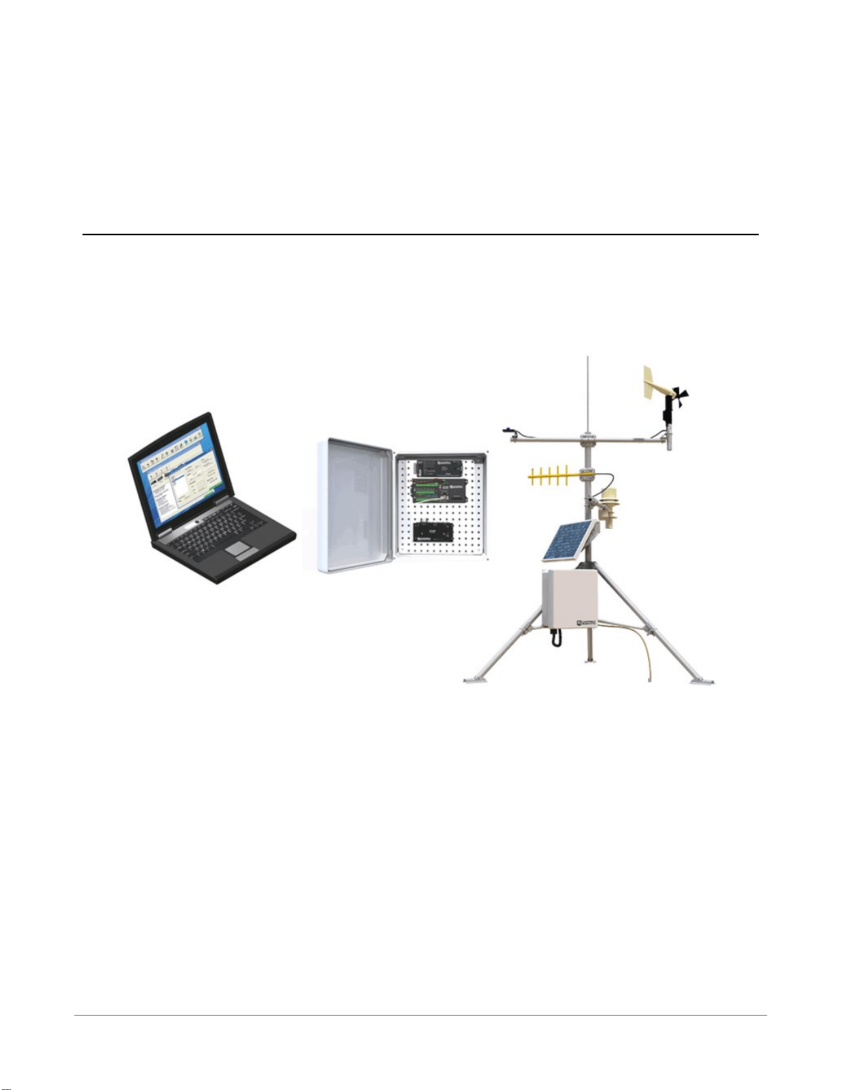
1. GRANITE 6 data acquisition system components

A basic data acquisition system consists of sensors, measurement hardware, and a computer with programmable software. The objective of a data acquisition system should be high accuracy, high precision, and resolution as high as appropriate for a given application.

The components of a basic data acquisition system are shown in the following figure.

Following is a list of typical data acquisition system components:

l Sensors - Electronic sensors convert the state of a phenomenon to an electrical signal (see

Sensors (p. 3) for more information).

l Data logger - The data logger measures electrical signals or reads serial characters. It

converts the measurement or reading to engineering units, performs calculations, and reduces data to statistical values. Data is stored in memory to await transfer to a computer by way of an external storage device or a communications link.

l Data Retrieval and Communications - Data is copied (not moved) from the data logger,

usually to a computer, by one or more methods using data logger support software. Most communications options are bi-directional, which allows programs and settings to be sent to the data logger. For more information, see Sending a program to the data logger (p. 35).

1. GRANITE 6 data acquisition system components 1

l Datalogger Support Software - Software retrieves data, sends programs, and sets settings.

The software manages the communications link and has options for data display.

l Programmable Logic Control - Some data acquisition systems require the control of

external devices to facilitate a measurement or to control a device based on measurements. This data logger is adept at programmable logic control. See Programmable logic control (p. 18) for more information.

l Measurement and Control Peripherals - Sometimes, system requirements exceed the

capacity of the data logger. The excess can usually be handled by addition of input and output expansion modules.

l Campbell Distributed Module (CDM) - CDMs increase measurement capability can be

centrally located or distributed throughout the network. Modules are controlled and synchronized by a single GRANITE 6. GRANITE Measurement Modules are one type of CDM.

1.1 The GRANITE 6 Datalogger

The GRANITE 6 data logger provides fast communications, low power requirements, built-in USB, compact size and and high analogue input accuracy and resolution. It includes universal (U) terminals, which allow connection to virtually any sensor - analogue, digital, or smart. This multipurpose data logger is also capable of doing static vibrating-wire measurements.

1.1.1 Overview

The GRANITE 6 data logger is the main part of a data acquisition system (see GRANITE 6 data

acquisition system components (p. 1) for more information). It has a central-processing unit

(CPU), analogue and digital measurement inputs, analogue and digital outputs, and memory. An operating system (firmware) coordinates the functions of these parts in conjunction with the onboard clock and the CRBasic application program.

The GRANITE 6 can simultaneously provide measurement and communications functions. Low power consumption allows the data logger to operate for extended time on a battery recharged with a solar panel, eliminating the need for ac power. The GRANITE 6 temporarily suspends operations when primary power drops below 9.6 V, reducing the possibility of inaccurate measurements.

1.1.2 Operations

The GRANITE 6 measures almost any sensor with an electrical response, drives direct communications and telecommunications, reduces data to statistical values, performs calculations, and controls external devices. After measurements are made, data is stored in onboard, nonvolatile memory. Because most applications do not require that every measurement

1. GRANITE 6 data acquisition system components 2

be recorded, the program usually combines several measurements into computational or statistical summaries, such as averages and standard deviations.

1.1.3 Programs

A program directs the data logger on how and when sensors are measured, calculations are made, data is stored, and devices are controlled. The application program for the GRANITE 6 is written in CRBasic, a programming language that includes measurement, data processing, and analysis routines, as well as the standard BASIC instruction set. For simple applications, Short Cut, a user-friendly program generator, can be used to generate the program. For more demanding programs, use the full featured CRBasic Editor.

Programs are run by the GRANITE 6 in either sequential mode or pipeline mode. In sequential mode, each instruction is executed sequentially in the order it appears in the program. In pipeline mode, the GRANITE 6 determines the order of instruction execution to maximize efficiency.

1.2 Sensors

Sensors transduce phenomena into measurable electrical forms by modulating voltage, current, resistance, status, or pulse output signals. Suitable sensors do this with accuracy and precision. Smart sensors have internal measurement and processing components and simply output a digital value in binary, hexadecimal, or ASCII character form.

Most electronic sensors, regardless of manufacturer, will interface with the data logger. Some sensors require external signal conditioning. The performance of some sensors is enhanced with specialized input modules. The data logger, sometimes with the assistance of various peripheral devices, can measure or read nearly all electronic sensor output types.

The following list may not be comprehensive. A library of sensor manuals and application notes is available at www.campbellsci.eu/support to assist in measuring many sensor types.

l Analogue

Voltage

Current

Strain

Thermocouple

Resistive bridge

l Pulse

High frequency

Switch-closure

1. GRANITE 6 data acquisition system components 3

Low-level ac

Quadrature

l Period average l Vibrating wire l Smart sensors

SDI-12

RS-232

Modbus

DNP3

TCP/IP

RS-422

RS-485

1. GRANITE 6 data acquisition system components 4

2. Wiring panel and terminal functions

The GRANITE 6 wiring panel provides ports and removable terminals for connecting sensors, power, and communications devices. It is protected against surge, over-voltage, over-current, and reverse power. The wiring panel is the interface to most data logger functions so studying it is a good way to get acquainted with the data logger. Functions of the terminals are broken down into the following categories:

l Analogue input l Pulse counting l Analogue output l Communications l Digital I/O l Power input l Power output l Power ground l Signal ground

2. Wiring panel and terminal functions 5

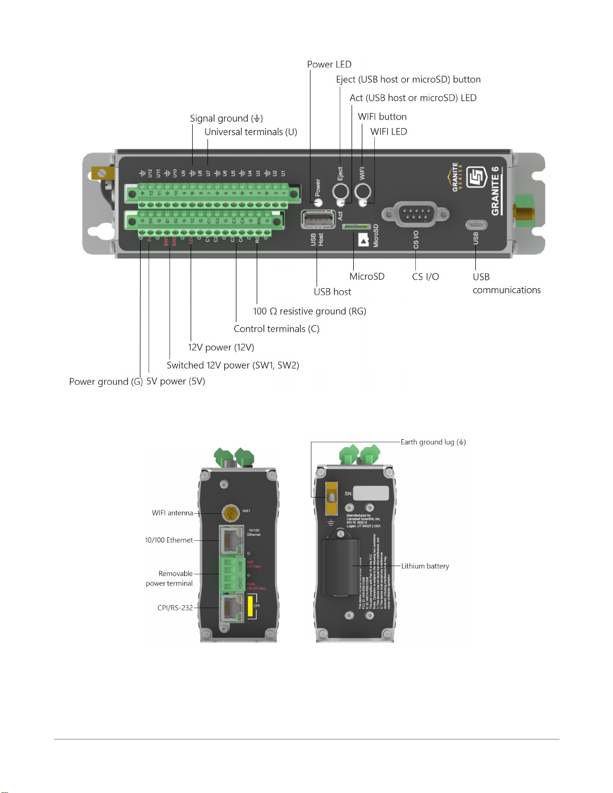
FIGURE 2-1. GRANITE 6 Wiring panel

FIGURE 2-2. GRANITE 6

2. Wiring panel and terminal functions 6

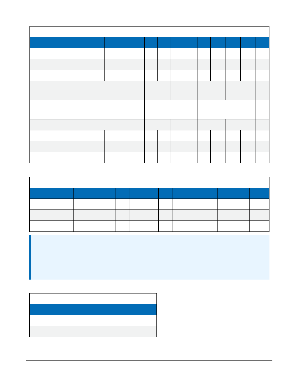
Table 2-1: Analogue input terminal functions

U1 U2 U3 U4 U5 U6 U7 U8 U9 U10 U11 U12 RG

Single-Ended Voltage ✓ ✓ ✓ ✓ ✓ ✓ ✓ ✓ ✓ ✓ ✓ ✓

Differential Voltage H L H L H L H L H L H L

Ratiometric/Bridge ✓ ✓ ✓ ✓ ✓ ✓ ✓ ✓ ✓ ✓ ✓ ✓

Vibrating Wire (Static,

✓ ✓ ✓ ✓ ✓ ✓

VSPECT®)

Vibrating Wire with

✓ ✓ ✓

Thermistor

Thermistor ✓ ✓ ✓ ✓ ✓ ✓

Thermocouple ✓ ✓ ✓ ✓ ✓ ✓ ✓ ✓ ✓ ✓ ✓ ✓

Current Loop ✓

Period Average ✓ ✓ ✓ ✓ ✓ ✓ ✓ ✓ ✓ ✓ ✓ ✓

Table 2-2: Pulse counting terminal functions

U1 U2 U3 U4 U5 U6 U7 U8 U9 U10 U11 U12 C1-C4

Switch-Closure ✓ ✓ ✓ ✓ ✓ ✓ ✓ ✓ ✓ ✓ ✓ ✓ ✓

High Frequency ✓ ✓ ✓ ✓ ✓ ✓ ✓ ✓ ✓ ✓ ✓ ✓ ✓

Low-level Ac ✓ ✓ ✓ ✓ ✓ ✓

NOTE: Conflicts can occur when a control port pair is used for different instructions (TimerInput(),

PulseCount(), SDI12Recorder(), WaitDigTrig()). For example, if C1 is used for SDI12Recorder(), C2 cannot be used for TimerInput(), PulseCount(), or WaitDigTrig().

Table 2-3: Analogue output terminal functions

U1-U12

Switched Voltage Excitation ✓

Switched Current Excitation ✓

2. Wiring panel and terminal functions 7

Table 2-4: Voltage output terminal functions

U1-U12 C1-C4 12V SW12-1 SW12-2 5V

3.3 VDC ✓ ✓

5 VDC ✓ ✓ ✓

12 VDC ✓ ✓ ✓

C and even numbered U terminals have limited drive capacity. Voltage levels are configured in pairs.

Table 2-5: Communications terminal functions

U1 U2 U3 U4 U5 U6 U7 U8 U9 U10 U11 U12 C1 C2 C3 C4

SDI-12 ✓ ✓ ✓ ✓ ✓ ✓ ✓ ✓

GPS

Time

Sync

PPS Rx Tx Rx Tx Rx

RS-

232/

CPI

TTL

Tx Rx Tx Rx Tx Rx Tx Rx Tx Rx Tx Rx Tx Rx Tx Rx

0-5 V

LVTTL

Tx Rx Tx Rx Tx Rx Tx Rx Tx Rx Tx Rx Tx Rx Tx Rx

0-3.3 V

RS-232 Tx Rx Tx Rx ✓

RS-485

(Half

Duplex)

RS-485

(Full

Duplex)

I2C SCL SDA SCL SDA SCL SDA SCL SDA SCL SDA SCL SDA SCL SDA SCL SDA

SPI MOSI SCLK MISO MOSI SCLK MISO MOSI SCLK MISO MOSI SCLK MISO

A- B+ A- B+

Tx- Tx+ Rx- Rx+

2. Wiring panel and terminal functions 8

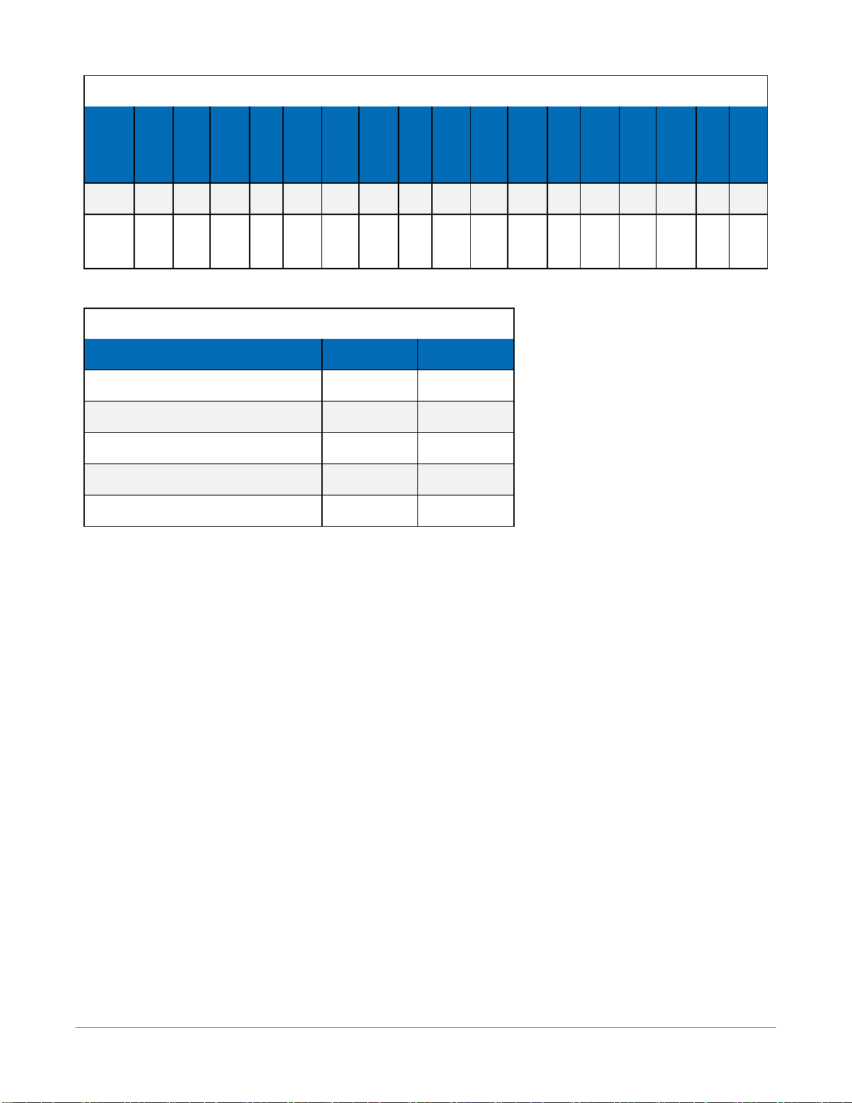
Table 2-5: Communications terminal functions

U1 U2 U3 U4 U5 U6 U7 U8 U9 U10 U11 U12 C1 C2 C3 C4

SDM Data Clk Enabl Data Clk Enabl Data Clk Enabl Data Clk Enabl

RS-

232/

CPI

CPI/

CDM

Table 2-6: Digital I/O terminal functions

U1-U12 C1-C4

General I/O ✓ ✓

Pulse-Width Modulation Output ✓ ✓

Timer Input ✓ ✓

Interrupt ✓ ✓

Quadrature ✓ ✓

2.1 Power input

The data logger requires a power supply. It can receive power from a variety of sources, operate for several months on non-rechargeable batteries, and supply power to many sensors and devices. The data logger operates with external power connected to the green BAT and/or CHG terminals on the side of the module. The positive power wire connects to +. The negative wire connects to -. The power terminals are internally protected against polarity reversal and high voltage transients.

✓

In the field, the data logger can be powered in any of the following ways:

l 10 to 18 VDC applied to the BAT + and – terminals l 16 to 32 VDC applied to the CHG + and – terminals

To establish an uninterruptible power supply (UPS), connect the primary power source (often a transformer, power converter, or solar panel) to the CHG terminals and connect a nominal 12 VDC sealed rechargeable lead-acid battery to the BAT terminals. See Power budgeting (p. 117) for more information. The Status Table ChargeState may display any of the following:

2. Wiring panel and terminal functions 9

l No Charge - The charger input voltage is either less than +9.82V±2% or there is no charger

attached to the terminal block.

l Low Charge Input – The charger input voltage is less than the battery voltage. l Current Limited – The charger input voltage is greater than the battery voltage AND the

battery voltage is less than the optimal charge voltage. For example, on a cloudy day, a solar panel may not be providing as much current as the charger would like to use.

l Float Charging – The battery voltage is equal to the optimal charge voltage. l Regulator Fault - The charging regulator is in a fault condition.

WARNING: Sustained input voltages in excess of 32 VDC on CHGor BAT terminals can damage the transient voltage suppression.

Ensure that power supply components match the specifications of the device to which they are connected. When connecting power, switch off the power supply, insert the connector, then turn the power supply on. See Troubleshooting power supplies (p. 133) for more information.

Following is a list of GRANITE 6 power input terminals and the respective power types supported.

l BAT terminals: Voltage input is 10 to 18 VDC. This connection uses the least current since

the internal data logger charging circuit is bypassed. If the voltage on the BAT terminals exceeds 19 VDC, power is shut off to certain parts of the data logger to prevent damaging connected sensors or peripherals.

l CHG terminals: Voltage input range is 16 to 32 VDC. Connect a primary power source, such

as a solar panel or VAC-to-VDC transformer, to CHG. The voltage applied to CHG terminals must be at least 0.3 V higher than that needed to charge a connected battery. When within the 16 to 32 VDC range, it will be regulated to the optimal charge voltage for a lead acid battery at the current data logger temperature, with a maximum voltage of approximately 15 VDC. A battery need not be connected to the BAT terminals to supply power to the data logger through the CHG terminals. The onboard charging regulator is designed for efficiently charging lead-acid batteries. It will not charge lithium or alkaline batteries.

l USB Device port: 5 VDC via USB connection. If power is also provided with BAT or CHG,

power will be supplied by whichever has the highest voltage. If USB is the only power source, then the CS I/O port and the 12V and SW12 terminals will not be operational. When powered by USB (no other power supplies connected) Status field Battery = 0. Functions that will be active with a 5 VDC source include sending programs, adjusting data logger settings, and making some measurements.

2. Wiring panel and terminal functions 10

NOTE: The Status field Battery value and the destination variable from the Battery() instruction (often called batt_volt or BattV) in the Public table reference the external battery voltage. For information about the internal battery, see Internal battery (p. 114).

2.1.1 Powering a data logger with a vehicle

If a data logger is powered by a motor-vehicle power supply, a second power supply may be needed. When starting the motor of the vehicle, battery voltage often drops below the voltage required for data logger operation. This may cause the data logger to stop measurements until the voltage again equals or exceeds the lower limit. A second supply or charge regulator can be provided to prevent measurement lapses during vehicle starting.

In vehicle applications, the earth ground lug should be firmly attached to the vehicle chassis with 12 AWG wire or larger.

2.1.2 Power LED indicator

When the data logger is powered, the Power LED will turn on according to power and program states:

l Off: No power, no program running. l 1 flash every 10 seconds: Powered from BAT, program running. l 2 flashes every 10 seconds: Powered from CHG, program running. l 3 flashes every 10 seconds: Powered via USB, program running. l Always on: Powered, no program running.

2.2 Power output

The data logger can be used as a power source for communications devices, sensors and peripherals. Take precautions to prevent damage to these external devices due to over- or undervoltage conditions, and to minimize errors. Additionally, exceeding current limits causes voltage output to become unstable. Voltage should stabilize once current is again reduced to within stated limits. The following are available:

l 12V: unregulated nominal 12 VDC. This supply closely tracks the primary data logger supply

voltage; so, it may rise above or drop below the power requirement of the sensor or peripheral. Precautions should be taken to minimize the error associated with measurement of underpowered sensors.

2. Wiring panel and terminal functions 11

l 5V: regulated 5 VDC. The 5 VDC supply is regulated to within a few millivolts of 5 VDC as

long as the main power supply for the data logger does not drop below the minimum supply voltage. It is intended to power sensors or devices requiring a 5 VDC power supply. It is not intended as an excitation source for bridge measurements. Current output is shared with the CSI/O port; so, the total current must be within the current limit.

SW12: program-controlled, switched 12 VDC terminals. It is often used to power devices

such as sensors that require 12 VDC during measurement. Voltage on a SW12 terminal will change with data logger supply voltage. CRBasic instruction SW12()controls the SW12 terminal. See the CRBasic Editor help for detailed instruction information and program examples: https://help.campbellsci.eu/crbasic/granite6/.

l CS I/O port: used to communicate with and often supply power to Campbell Scientific

peripheral devices.

CAUTION: Voltage levels at the 12V and switched SW12 terminals, and pin 8 on the CS I/O port, are tied closely to the voltage levels of the main power supply. Therefore, if the power received at the POWER IN 12V and G terminals is 16 VDC, the 12V and SW12 terminals and pin 8 on the CS I/O port will supply 16 VDC to a connected peripheral. The connected peripheral or sensor may be damaged if it is not designed for that voltage level.

l C or U terminals: can be set low or high as output terminals . With limited drive capacity,

digital output terminals are normally used to operate external relay-driver circuits. Drive current varies between terminals. See also Digital input/output specifications (p. 199).

l U terminals: can be configured to provide regulated ±2500 mV dc excitation.

See also Power output specifications (p. 190).

2.3 Grounds

Proper grounding lends stability and protection to a data acquisition system. Grounding the data logger with its peripheral devices and sensors is critical in all applications. Proper grounding will ensure maximum ESD protection and measurement accuracy. It is the easiest and least expensive insurance against data loss, and often the most neglected. The following terminals are provided for connection of sensor and data logger grounds:

Signal Ground ( ) - reference for single-ended analogue inputs, excitation returns,

and a ground for sensor shield wires.

6 common terminals

2. Wiring panel and terminal functions 12

l Power Ground (G) - return for 3.3 V, 5 V, 12 V, U or C terminals configured for control, and

digital sensors. Use of G grounds for these outputs minimizes potentially large current flow through the analogue-voltage-measurement section of the wiring panel, which can cause single-ended voltage measurement errors.

6 common terminals

l Resistive Ground (RG) - used for non-isolated 0-20 mA and 4-20 mA current loop

measurements (see Current-loop measurements (p. 56) for more information). Also used for decoupling ground on RS-485 signals. Includes 100 Ω resistance to ground. Maximum voltage for RG terminal is ±16 V.

1 terminal

l Earth Ground Lug ( ) - connection point for heavy-gauge earth-ground wire. A good earth

connection is necessary to secure the ground potential of the data logger and shunt transients away from electronics. Campbell Scientific recommends 14 AWG wire, minimum.

NOTE: Several ground wires can be connected to the same ground terminal.

A good earth (chassis) ground will minimize damage to the data logger and sensors by providing a low-resistance path around the system to a point of low potential. Campbell Scientific recommends that all data loggers be earth grounded. All components of the system (data loggers, sensors, external power supplies, mounts, housings) should be referenced to one common earth ground.

In the field, at a minimum, a proper earth ground will consist of a 5-foot copper-sheathed grounding rod driven into the earth and connected to the large brass ground lug on the wiring panel with a 14 AWG wire. In low-conductive substrates, such as sand, very dry soil, ice, or rock, a single ground rod will probably not provide an adequate earth ground. For these situations, search for published literature on lightning protection or contact a qualified lightning-protection consultant.

In laboratory applications, locating a stable earth ground is challenging, but still necessary. In older buildings, new VAC receptacles on older VAC wiring may indicate that a safety ground exists when, in fact, the socket is not grounded. If a safety ground does exist, good practice dictates to verify that it carries no current. If the integrity of the VAC power ground is in doubt, also ground the system through the building plumbing, or use another verified connection to earth ground.

2.4 Communications ports

The data logger is equipped with ports that allow communications with other devices and networks, such as:

l Computers l Smart sensors l Modbus and DNP3 networks l Ethernet l Modems l Campbell Scientific PakBus® networks l Other Campbell Scientific data loggers l GRANITE Measurement Modules

Campbell Scientific data logger communications ports include:

l CS I/O l CPI/RS-232 l USB Device l USB Host l Ethernet l C and U terminals

2.4.1 USB device port

One USB device port supports communicating with a computer through data logger support software or through virtual Ethernet (RNDIS), and provides 5 VDC power to the data logger (powering through the USB port has limitations - details are available in the specifications). The data logger USB device port does not support USBflash or thumb drives; use the USB host port for these external devices. Although the USB connection supplies 5 V power, a 12 VDC battery will be needed for field deployment.

2.4.2 USB host port

USB host provides portable data storage on a mass storage device (MSD). A single USB thumb drive can be inserted into the drive and will show up as a drive (USB: ) in file related operations. Measurement data is stored on USB: as discrete files by using the TableFile() instruction. Files on USB can be collected by inserting the thumb drive into a computer and copying the files.

USB: can be used in the TableFile() instruction and all file access related instructions in CRBasic. Because of data-reliability concerns in non-industrial rated drives, this drive is not intended for long term unattended data storage. USB: is not affected by program recompilation or formatting of other drives.

2. Wiring panel and terminal functions 14

2.4.3 Ethernet port

The RJ45 10/100 Ethernet port is used for IP communications.

2.4.4 C and U terminals for communications

C and U terminals are configurable for the following communications types:

l SDI-12 l RS-232 l RS-422 l RS-485 l TTL (0 to 5 V) l LVTTL (0 to 3.3 V) l SDM

Some communications types require more than one terminal, and some are only available on specific terminals. This is shown in the data logger specifications.

2.4.4.1 SDI-12 ports

SDI-12 is a 1200 baud protocol that supports many smart sensors. C1, C3, U1, U3, U5, U7, U9, and U11 can each be configured as SDI-12 ports. Maximum cable lengths depend on the number of sensors connected, the type of cable used, and the environment of the application. Refer to the sensor manual for guidance.

For more information, see SDI-12 communications (p. 101).

2.4.4.2 RS-232, RS-422, RS-485, TTL, and LVTTL ports

RS-232, RS-422, RS-485, TTL, and LVTTL communications are typically used for the following:

l Reading sensors with serial output l Creating a multi-drop network l Communications with other data loggers or devices over long cables

Configure C or U terminals as serial ports using Device Configuration Utility or by using the

SerialOpen() CRBasic instruction. C and U terminals are configured in pairs for TTL and

LVTTL communications, and C terminals are configured in pairs for RS-232 or half-duplex RS-422 and RS-485. For full-duplex RS-422 and RS-485, all four C terminals are required. See also

Communications protocols (p. 80).

NOTE: RS-232 ports are not isolated.

2. Wiring panel and terminal functions 15

2.4.4.3 SDM ports

SDM is a protocol proprietary to Campbell Scientific that supports several Campbell Scientific digital sensor and communications input and output expansion peripherals and select smart sensors. It uses a common bus and addresses each node. CRBasic SDM device and sensor instructions configure terminals C1, C2, and C3 together to create an SDM port. Alternatively, terminals U1, U2, and U3; U5, U6, and U7; or U9, U10, and U11 can be configured together to be used as SDM ports by using the SDMBeginPort()instruction.

See also Communications specifications (p. 201).

2.4.5 CS I/O port

One nine-pin port, labelled CS I/O, is available for communicating with a computer through Campbell Scientific communications interfaces, modems, and peripherals. Campbell Scientific recommends keeping CS I/O cables short (maximum of a few feet). See also Communications

specifications (p. 201).

Table 2-7: CS I/O pinout

Function

Number

1 5 VDC O 5 VDC: sources 5 VDC, used to power peripherals.

2 SG

3 RING I

4 RXD I

5 ME O

6 SDE O

7 CLK/HS I/O

Input(I)

Description

Output(O)

Signal ground: provides a power return for pin 1 (5V), and is used as a reference for voltage levels.

Ring: raised by a peripheral to put the GRANITE 6 in the telecom mode.

Receive data: serial data transmitted by a peripheral are received on pin 4.

Modem enable: raised when the GRANITE 6 determines that a modem raised the ring line.

Synchronous device enable: addresses synchronous devices (SD); used as an enable line for printers.

Clock/handshake: with the SDE and TXD lines addresses and transfers data to SDs. When not used as a clock, pin 7 can be used as a handshake line; during printer output, high enables, low disables.

2. Wiring panel and terminal functions 16

Table 2-7: CS I/O pinout

Function

Number

Input(I)

Description

Output(O)

Nominal 12 VDC power. Same power as 12V and SW12

8 12VDC

terminals.

Transmit data: transmits serial data from the data logger to peripherals on pin 9; logic-low marking (0V), logichigh spacing (5V), standard-asynchronous ASCII: eight

9 TXD O

data bits, no parity, one start bit, one stop bit. User selectable baud rates: 300, 1200, 2400, 4800, 9600, 19200, 38400, 115200.

2.4.6 CPI/RS-232 port

The data logger includes one RJ45 module jack labelled RS-232/CPI. CPI is a proprietary interface for communications between Campbell Scientific data loggers and Campbell Distributed Modules (CDMs) such as the GRANITE-Series peripheral devices and smart sensors. It consists of a physical layer definition and a data protocol. CDM devices are similar to Campbell Scientific SDM devices in concept, but the CPI bus enables higher data-throughput rates and use of longer cables. Some GRANITE devices may require more power to operate in general than do SDM devices. Consult the manuals for GRANITE modules for more information.

NOTE: CPI/RS-232 port is not isolated.

CPI port power levels are controlled automatically by the GRANITE 6:

l Off: Not used. l High power: Fully active. l Low-power standby: Used whenever possible. l Low-power bus: Sets bus and modules to low power.

When used with a Campbell Scientific RJ45-to-DB9 converter cable, the CPI/RS-232 port can be used as an RS-232 port. It defaults to 115200 bps (in autobaud mode), 8 data bits, no parity, and 1 stop bit. Use Device Configuration Utility or the SerialOpen() CRBasic instruction to change these options.

2. Wiring panel and terminal functions 17

Table 2-8: RS-232/CPI pinout

Pin Number Description

1 RS-232: Transmit (Tx)

2 RS-232: Receive (Rx)

3 100 Ω Res Ground

4 CPI: Data

5 CPI: Data

6 100 Ω Res Ground

7 RS-232 CTS CPI: Sync

8 RS-232 DTR CPI: Sync

9 Not Used

2.5 Programmable logic control

The data logger can control instruments and devices such as:

l Controlling cellular modem or GPS receiver to conserve power. l Triggering a water sampler to collect a sample. l Triggering a camera to take a picture. l Activating an audio or visual alarm. l Moving a head gate to regulate water flows in a canal system. l Controlling pH dosing and aeration for water quality purposes. l Controlling a gas analyzer to stop operation when temperature is too low. l Controlling irrigation scheduling.

Control decisions can be based on time, an event, or a measured condition. Controlled devices can be physically connected to C, U, or SW12 terminals. Short Cut has provisions for simple on/off control. Control modules and relay drivers are available to expand and augment data logger control capacity.

C and U terminals are selectable as binary inputs, control outputs, or communication ports.

These terminals can be set low (0 VDC) or high (3.3 or 5 VDC) using the PortSet()or

WriteIO() instructions. See the CRBasic Editor help for detailed instruction information

and program examples: https://help.campbellsci.eu/crbasic/granite6/. Other functions include device-driven interrupts, asynchronous communications and SDI-12 communications. The high voltage for these terminals defaults to 5 V, but it can be

2. Wiring panel and terminal functions 18

changed to 3.3 V using the PortPairConfig() instruction. A C or U terminal configured for digital I/O is normally used to operate an external relay-driver circuit because the terminal itself has limited drive capacity.

l SW12 terminals can be set low (0 V) or high (12 V) using the SW12() instruction (see the

CRBasic help for more information).

The following image illustrates a simple application wherein a C or Uterminal configured for digital input, and another configured for control output are used to control a device (turn it on or off) and monitor the state of the device (whether the device is on or off).

In the case of a cell modem, control is based on time. The modem requires 12 VDC power, so connect its power wire to a data logger SW12 terminal. The following code snip turns the modem on for the first ten minutes of every hour using the TimeIsBetween() instruction embedded in an If/Then logic statement:

If TimeIsBetween (0,10,60,Min)Then

SW12(SW12_1,1,1) 'Turn phone on.

Else

SW12(SW12_1,0,1) 'Turn phone off.

EndIf

2. Wiring panel and terminal functions 19

3. Setting up the GRANITE 6

The basic steps for setting up your data logger to take measurements and store data are included in the following sections:

3.1 Setting up communications with the data logger 20

3.2 Testing communications with EZSetup 30

3.3 Making the software connection 31

3.4 Programming quickstart using Short Cut 32

3.5 Sending a program to the data logger 35

3.1 Setting up communications with the data logger

The first step in setting up and communicating with your data logger is to configure your connection. Communications peripherals, data loggers, and software must all be configured for communications. Additional information is found in your specific peripheral manual, and the data logger support software manual and help.

The default settings for the data logger allow it to communicate with a computer via USB, RS232, or Ethernet. For other communications methods or more complex applications, some settings may need adjustment. Settings can be changed through Device Configuration Utility or through data logger support software.

You can configure your connection using any of the following options. The simplest is via USB. For detailed instruction, see:

3.1.1 USB or RS-232 communications 21

3.1.2 Virtual Ethernet over USB (RNDIS) 22

3.1.3 Ethernet communications option 23

3.1.4 Wi-Fi communications 26

For other configurations, see the LoggerNet EZSetup Wizard help. Context-specific help is given in each step of the wizard by clicking the Help button in the bottom right corner of the window. For complex data logger networks, use Network Planner. For more information on using the

3. Setting up the GRANITE 6 20

Network Planner, watch a video at https://www.campbellsci.eu/videos/loggernet-software-

network-planner .

3.1.1 USB or RS-232 communications

Setting up a USB or RS-232 connection is a good way to begin communicating with your data logger. Because these connections do not require configuration (like an IPaddress), you need only set up the communications between your computer and the data logger. Use the following instructions or watch the Quickstart videos at https://www.campbellsci.eu/videos .

Follow these steps to get started. These settings can be revisited using the data logger support software Edit Datalogger Setup option .

1. Using data logger support software, launch the EZSetup Wizard.

LoggerNet users, click Setup , click the View menu to ensure you are in the EZ (Simplified) view, then click Add Datalogger.

RTDAQ users, click Add Datalogger .

2. Click Next.

3. Select your data logger from the list, type a name for your data logger (for example, a site or project name), and click Next.

4. If prompted, select the Direct Connect connection type and click Next.

5. If this is the first time connecting this computer to a GRANITE 6 via USB, click Install USBDriver, select your data logger, click Install, and follow the prompts to install the USBdrivers.

6. Plug the data logger into your computer using a USBor RS-232 cable. The USB connection supplies 5 V power as well as a communications link, which is adequate for setup. A 12V battery will be needed for field deployment. If using RS-232, external power must be provided to the data logger and a CPI/RS-232 RJ45 to DB9 cable is required to connect to the computer.

NOTE: The Power LED on the data logger indicates the program and power state. Because the data logger ships with a program set to run on power-up, the Power LED flashes 3 times every 10 seconds when powered over USB. When powered with a 12 V battery, it flashes 1 time every 10 seconds.

7. From the COM Port list, select the COMport used for your data logger.

3. Setting up the GRANITE 6 21

8. USB and RS-232 connections do not typically require a COM Port Communication Delay this allows time for the hardware devices to "wake up" and negotiate a communications link. Accept the default value of 00 seconds and click Next.

9. The baud rate and PakBus address must match the hardware settings for your data logger. The default PakBus address is 1. A USB connection does not require a baud rate selection. RS-232 connections default to 115200 baud.

10. Set an Extra Response Time if you have a difficult or marginal connection and you want the data logger support software to wait a certain amount of time before returning a communication failure error.

11. LoggerNet users can set a Max Time On-Line to limit the amount of time the data logger remains connected. When the data logger is contacted, communication with it is terminated when this time limit is exceeded. A value of 0 in this field indicates that there is no time limit for maintaining a connection to the data logger.

12. Click Next.

13. By default, the data logger does not use a security code or a PakBus encryption key. Therefore, the Security Code can be set to 0 and the PakBus Encryption Key can be left blank. If either setting has been changed, enter the new code or key. See Data logger

security (p. 108) for more information.

14. Click Next.

15. Review the Setup Summary. If you need to make changes, click Previous to return to a previous window and change the settings.

Setup is now complete, and the EZSetup Wizard allows to you click Finish or click Next to test communications, set the data logger clock, and send a program to the data logger. See Testing

communications with EZSetup (p. 30) for more information.

3.1.2 Virtual Ethernet over USB (RNDIS)

GRANITE 6 data loggers support RNDIS (virtual Ethernet over USB). This allows the data logger to communicate via TCP/IP over USB. Watch a video

https://www.campbellsci.eu/videos/ethernet-over-usb or use the following instructions.

3. Setting up the GRANITE 6 22

1. Supply power to the data logger. If connecting via USB for the first time, you must first install USB drivers by using Device Configuration Utility (select your data logger, then on the main page, click Install USBDriver). Alternately, you can install the USBdrivers using EZ Setup. A USB connection supplies 5 V power (as well as a communication link), which is adequate for setup, but a 12 V battery will be needed for field deployment.

NOTE: Ensure the data logger is connected directly to the computer USB port (not to a USBhub). We recommended always using the same USB port on your computer.

2. Physically connect your data logger to your computer using a USB cable, then in Device Configuration Utility select your data logger.

3. Retrieve your IPAddress. On the bottom, left side of the screen, select IP as the Connection Type, then click the browse button next to the Server Address box. Note the IP Address (default is 192.168.66.1). If you have multiple data loggers in your network, more than one data logger may be returned. Ensure you select the correct data logger by verifying the data logger serial number or station name (if assigned).

4. A virtual IP address can be used to connect to the data logger using Device Configuration Utility or other computer software, or to view the data logger internal web page in a

browser. To view the web page, open a browser and enter linktodevice.eu or the IP address you retrieved in the previous step (for example, 192.168.66.1) into the address bar.

To secure your data logger from others who have access to your network, we recommend that you set security. For more information, see Data logger security (p. 108).

NOTE: Ethernet over USB (RNDIS) is considered a direct communications connection. Therefore, it is a trusted connection and csipasswd does not apply.

3.1.3 Ethernet communications option

The GRANITE 6 offers a 10/100 Ethernet connection. Use Device Configuration Utility to enter the data logger IPAddress, Subnet Mask, and IPGateway address. After this, use the EZSetup Wizard to set up communications with the data logger. If you already have the data logger IPinformation, you can skip these steps and go directly to Setting up Ethernet communications

between the data logger and computer (p. 25). Watch a video https://www.campbellsci.eu/videos/datalogger-ethernet-configuration or use the following

instructions.

3. Setting up the GRANITE 6 23

3.1.3.1 Configuring data logger Ethernet settings

2. Connect an Ethernet cable to the 10/100 Ethernet port on the data logger. The yellow and green Ethernet port LEDs display activity approximately one minute after connecting. If you do not see activity, contact your network administrator. For more information, see Ethernet

LEDs (p. 25).

3. Using data logger support software (LoggerNet or RTDAQ), open Device Configuration

Utility .

4. Select the GRANITE 6 data logger from the list

5. Select the port assigned to the data logger from the Communication Port list. If connecting via Ethernet, select Use IPConnection.

6. By default, this data logger does not use a PakBus encryption key; so, the PakBus Encryption Key box can be left blank. If this setting has been changed, enter the new code or key. See Data logger security (p. 108) for more information.

7. Click Connect.

8. On the Deployment tab, click the Ethernet subtab.

9. The Ethernet Power setting allows you to reduce the power consumption of the data logger. If there is no Ethernet connection, the data logger will turn off its Ethernet interface for the time specified before turning it back on to check for a connection. Select Always On, 1 Minute, or Disable.

10. Enter the IP Address, Subnet Mask, and IP Gateway. These values should be provided by your network administrator. A static IP address is recommended. If you are using DHCP, note the IP address assigned to the data logger on the right side of the window. When the IP Address is set to the default, 0.0.0.0, the information displayed on the right side of the window updates with the information obtained from the DHCP server. Note, however, that this address is not static and may change. An IP address here of 169.254.###.### means the data logger was not able to obtain an address from the DHCP server. Contact your network administrator for help.

11. Apply to save your changes.

3. Setting up the GRANITE 6 24

3.1.3.2 Ethernet LEDs

When the data logger is powered, and Ethernet Power setting is not disabled, the 10/100 Ethernet LEDs will show the Ethernet activity:

l Solid Yellow: Valid Ethernet link. l No Yellow: Invalid Ethernet link. l Flashing Yellow: Ethernet activity. l Solid Green: 100 Mbps link. l No Green: 10 Mbps link.

3.1.3.3 Setting up Ethernet communications between the data logger and computer

Once you have configured the Ethernet settings or obtained the IPinformation for your data logger, you can set up communications between your computer and the data logger over Ethernet. Watch a video https://www.campbellsci.eu/videos/ezsetup-ethernet-connection or use the following instructions.

This procedure only needs to be followed once per data logger. However, these settings can be revised using the data logger support software Edit Datalogger Setup option .

1. Using data logger support software, open EZSetup.

LoggerNet users, select Setup from the Main category on the toolbar, click the View menu to ensure you are in the EZ(Simplified) view, then click Add Datalogger.

RTDAQ users, click Add Datalogger .

2. Click Next.

3. Select the GRANITE 6 from the list, enter a name for your station (for example, a site or project name), Next.

4. Select the IPPort connection type and click Next.

5. Type the data logger IPaddress followed by a colon, then the port number of the data logger in the Internet IPAddress box (these were set up through the Ethernet

communications option (p. 23)) step. They can be accessed in Device Configuration Utility

on the Ethernet subtab. Leading 0s must be omitted. For example:

l IPv4 addresses are entered as 192.168.1.2:6785

l IPv6 addresses must be enclosed in square brackets. They are entered as

[2001:db8::1234:5678]:6785

3. Setting up the GRANITE 6 25

6. The PakBus address must match the hardware settings for your data logger. The default PakBus address is1.

l Set an Extra Response Time if you want the data logger support software to wait a

certain amount of time before returning a communications failure error.

l LoggerNet users can set a Max Time On-Line to limit the amount of time the data

logger remains connected. When the data logger is contacted, communications with it is terminated when this time limit is exceeded. A value of 0 in this field indicates that there is no time limit for maintaining a connection to the data logger. Next.

7. By default, the data logger does not use a security code or a PakBus encryption key. Therefore the Security Code can be set to 0 and the PakBus Encryption Key can be left blank. If either setting has been changed, enter the new code or key. See Data logger

security (p. 108). Next.

8. Review the Communication Setup Summary. If you need to make changes, click Previous to return to a previous window and change the settings.

Setup is now complete, and the EZSetup Wizard allows you Finish or select Next. The Next steps take you through testing communications, setting the data logger clock, and sending a program to the data logger. See Testing communications with EZSetup (p. 30) for more information.

3.1.4 Wi-Fi communications

By default, the GRANITE 6 is configured to host a Wi-Fi network. The LoggerLink mobile app for iOS and Android can be used to connect with a GRANITE 6. Up to eight devices can connect to a network created by a GRANITE 6. The setup follows the same steps shown in this video: CR6-WIFI

Datalogger - Setting Up a Network .

NOTE: The user is responsible for emissions if changing the antenna type or increasing the gain.

See also Communications specifications (p. 201).

3.1.4.1 Configuring the data logger to host a Wi-Fi network

By default, the GRANITE 6 is configured to host a Wi-Fi network. If the settings have changed, you can follow these instructions to reconfigure it.

1. Ensure your GRANITE 6 is connected to an antenna and power.

2. Using Device Configuration Utility, connect to the data logger.

3. On the Deployment tab, click the Wi-Fi sub-tab.

3. Setting up the GRANITE 6 26

4. In the Configuration list, select the Create a Network option.

5. Optionally, set security on the network to prevent unauthorized access by typing a password in the Password box (recommended).

6. Apply your changes.

3.1.4.2 Connecting your computer to the data logger over Wi-Fi

1. Open the Wi-Fi network settings on your computer.

2. Select the Wi-Fi-network hosted by the data logger. The default name is GRANITE 6 followed by the serial number of the data logger. In the previous image, the Wi-Fi network is CRxxx.

3. If you set a password, select the Connect Using a Security Key option (instead of a PIN) and type the password you chose.

4. Connect to this network.

3.1.4.3 Setting up Wi-Fi communications between the data logger and the data logger support software

Using LoggerNet click Add Datalogger to launch the EZSetup Wizard. For LoggerNet users, you must first click Setup , then View menu to ensure you are in the EZ (Simplified) view, then click Add Datalogger .

3. Setting up the GRANITE 6 27

2. Select the IPPort connection type and click Next.

3. In the Internet IPAddress field, type 192.168.67.1. This is the default data logger IPaddress created when the GRANITE 6 creates a network.

4. Click Next.

5. The PakBus address must match the hardware settings for your data logger. The default PakBus address is 1.

l Set an Extra Response Time if you want the data logger support software to wait a

certain amount of time before returning a communication failure error. This can usually be left at 00 seconds.

l You can set a Max Time On-Line to limit the amount of time the data logger remains

connected. When the data logger is contacted, communication with it is terminated when this time limit is exceeded. A value of 0 in this field indicates that there is no time limit for maintaining a connection to the data logger.

6. Click Next.

7. By default, the data logger does not use a security code or a PakBus encryption key. Therefore, the Security Code can be left at 0 and the PakBus Encryption Key can be left blank. If either setting has been changed, enter the new code or key. See Data logger

security (p. 108) for more information.

8. Click Next.

9. Review the Communication Setup Summary. If you need to make changes, click the Previous button to return to a previous window and change the settings.

Setup is now complete, and the EZSetup Wizard allows you click Finish or click Next to test communications, set the data logger clock, and send a program to the data logger. See Testing

communications with EZSetup (p. 30) for more information.

3.1.4.4 Configuring data loggers to join a Wi-Fi network

By default, the GRANITE 6 is configured to host a Wi-Fi network. To set it up to join a network:

1. Ensure your GRANITE 6 is connected to an antenna and power.

2. Using Device Configuration Utility, connect to the data logger.

3. On the Deployment tab, click the Wi-Fi sub-tab.

4. In the Configuration list, select the Join a Network option.

Next to the Network Name (SSID) box, click Browse to search for and select a Wi-Fi network. To join a hidden network, manually enter its SSID.

3. Setting up the GRANITE 6 28

6. If the network is a secured network, you must enter the password in the Password box and add any additional security in the Enterprise section of the window.

7. Enter the IP Address, Network Mask, and Gateway. These values should be provided by your network administrator. A static IP address is recommended.

l Alternatively, you can use an IP address assigned to the data logger via DHCP. To do

this, make sure the IP Address is set to 0.0.0.0. Click Apply to save the configuration changes. Then reconnect. The IP information obtained through DHCP is updated and displayed in the Status section of the Wi-Fi subtab. Note, however, that this address is not static and may change. An IP address here of

169.254.###.### means the data logger was not able to obtain an address from the DHCP server. Contact your network administrator for help.

8. Apply your changes.

9. For each data logger you want to connect to network, you must follow the instruction in

Setting up Wi-Fi communications between the data logger and the data logger support software (p. 27), using the IP address used to configure that data logger (step 7 in this

instruction).

3.1.4.5 Wi-Fi mode button

Configure the Wi-Fi mode button using Device Configuration Utility software.

Disable button - When this configuration is selected, pressing the button will have no effect on the operation of the device. The Wi-Fi network will continue to work as configured.

Temporarily enable Wi-Fi - When this configuration is selected, the normally disabled Wi-Fi network will be activated temporarily when the button is pressed.

Temporarily create a network - When this configuration is selected, the device will temporarily create a network when the button is pressed. If the Wi-Fi configuration is set to "Join a Network" then the temporarily created network will be an open network with the name GRANITE 6_[Serial Number]. If the Wi-Fi configuration is set to "Create a Network" then the configured Wi-Fi network will normally be disabled, and it will be activated temporarily when the button is pressed.

NOTE:

When the Wi-Fi configuration is set to "Create a Network" the device behaviour is the same for both button configurations.

3.1.4.6 Wi-Fi LED indicator

When the data logger is powered, the Wi-Fi LED will turn on according to Wi-Fi communication states:

3. Setting up the GRANITE 6 29

l Off: Insufficient power, Wi-Fi disabled, or data logger failed to join or create a network

(periodic retries will occur).

l Solid for 2 seconds: Attempting to join or create a network. l Flashing: Successfully joined or created a network. Flashes with network activity and once

every four seconds.

3.2 Testing communications with EZSetup

1. Using data logger support software EZSetup, access the Communication Test window. This window is accessed during EZ Setup (see USB or RS-232 communications (p. 21) for more information). Alternatively, you can double-click a data logger from the station list to open the EZ Setup Wizard and access the Communication Test step from the left side of the window.

2. Ensure the data logger is connected to the computer, select Yes to test communications, then click Next to initiate the test. To troubleshoot an unsuccessful test, see Tips and

troubleshooting (p. 124).

3. With a successful connection, the Datalogger Clock window displays the time for both the data logger and the computer.

3. Setting up the GRANITE 6 30

l The Adjusted Server Date/Time displays the current reading of the clock for the

computer or server running your data logger support software. If the Datalogger Date/Time and Adjusted Server Date/Time don't match, you can set the data logger clock to the Adjusted Server Date/Time by clicking Set Datalogger Clock.

l Use the Time Zone Offset to specify a positive or negative offset to apply to the

computer time when setting the data logger clock. This offset will allow you to set the clock for a data logger that needs to be set to a different time zone than the time zone of the computer (or to accommodate for changes in daylight saving time).

4. Click Next.

5. The data logger ships with a default GettingStarted program. If the data logger does not have a program, you can choose to send one by clicking Select and Send Program. Click Next.

6. LoggerNet only - Use the following instructions or watch the Scheduled/Automatic Data

Collection video :

l The Datalogger Table Output Files window displays the data tables available to be

collected from the data logger and the output file name. By default, all data tables set up in the data logger program will be included for collection. Make note of the Output File Name and location. Click Next.

l Check Scheduled Collection Enabled to have LoggerNet automatically collect data

from the data logger on the Collection Interval entered. When the Base Date and Time are in the past, scheduled collection will begin immediately after finishing the EZSetup wizard. Click Next twice.

7. Click Finish.

3.3 Making the software connection

Once you have configured your hardware connection (see Setting up communications with the

data logger (p. 20), your data logger and computer can communicate. You'll use the Connect

screen to send a program, set the clock, view real-time data, and manually collect data.

LoggerNet users, select Main and Connect on the LoggerNet toolbar, select the data logger from the Stations list, then Connect .

RTDAQ users, select the data logger from the list and click Connect .

To disconnect, click Disconnect .

For more information see the Connect Window Tutorial .

3. Setting up the GRANITE 6 31

3.4 Programming quickstart using Short Cut

Short Cut is an easy way to program the GRANITE data acquisition system to measure a sensor and assign wiring terminals. Short Cut is available as a download from

https://www.campbellsci.eu/shortcut. It is also included in installations of LoggerNet and

RTDAQ.

The following procedure shows using Short Cut to program the data logger to measure a typeT thermocouple on a VOLT 100 series.

1. Open Short Cut and click Create New Program.

2. Double-click your GRANITE data logger.

3. In the Available Sensors and Devices box, start typing GRANITE. You can also locate it in the Devices folder. Double click the GRANITE Measurement Module you are working with. Type the serial number located on the VOLT 100 series label. Optionally, type a name in the Module ID String if you want the module to have an ID. This is useful when multiple VOLT 100 series modules are connected to the GRANITE data logger.

4. In the Available Sensors and Devices box, type Type T. You can also locate the thermocouple in the Sensors > Temperature folder. Double click Type T Thermocouple. Type the number of type T thermocouples connected to the VOLT 100 series. The temperature defaults to degree C. This can be changed by clicking the Temperature units box and selecting one of the other options.

3. Setting up the GRANITE 6 32

5. Click on the Wiring tab to see how the sensor is to be wired to the VOLT 100 series. Click OK after wiring the thermocouple.

6. Repeat steps four and five for other sensors you want to measure. Click Next.

3. Setting up the GRANITE 6 33

7. In Output Setup, type the scan rate, a meaningful table name, and the Data Output Storage Interval.

8. Select the measurement and its associated output option.

9. Click Finish and save the program. Send the program just created to the GRANITE data logger if it is connected to the computer.

10. If the thermocouple is connected to the VOLT 100 series, check the output of the thermocouple in the data logger support software data display in LoggerNet or RTDAQ to make sure it is making reasonable measurements.

3. Setting up the GRANITE 6 34

3.5 Sending a program to the data logger

TIP: It is good practice is to always retrieve data from the data logger before sending a program; otherwise, data may be lost. See Collecting data (p. 37) for detailed instruction.

Some methods of sending a program give the option to retain data when possible. Regardless of the program upload tool used, data will be erased when a new program is sent if any change occurs to one or more data table structures in the following list:

l Data table name(s) l Data output interval or offset l Number of fields per record

l Number of bytes per field l Field type, size, name, or position l Number of records in table

Use the following instructions or watch the Quickstart part 3 video .

1. Connect the data logger to your computer (see Making the software connection (p. 31) for more information).

2. Using your data logger support software, click Send New... or Send Program (located in the Current Program section on the right side of the window).

3. Navigate to the program, select it, and click Open. For example: navigate to C:\Campbellsci\SCWin and select MyTemperature.CRB.

4. Confirm that you would like to proceed and erase all data tables saved on the data logger. The program will send and compile.

5. Review the Compile Results window for errors, messages and warnings.

6. Click Details, select the Table Fill Times tab. Ensure that the times shown are expected for your application. Click OK.

After sending a program, it is a good idea to monitor the Public Table to make sure sensors are taking good measurements. See Working with data (p. 36) for more information.

3. Setting up the GRANITE 6 35

4. Working with data

4.1 Default data tables

By default, the data logger includes three tables: Public, Status, and DataTableInfo. Each of these tables only contains the most recent measurements and information.

l The Public table is configured by the data logger program, and updated at the scan

interval set within the data logger program, It shows measurement and calculation results as they are made.

l The Status table includes information about the health of the data logger and is updated

only when viewed.

l The DataTableInfo table reports statistics related to data tables. It also only updates when

viewed.

l User-defined data tables update at the schedule set within the program.

For information on collecting your data, see Collecting data (p. 37).

Use these instructions or follow the Connect Window tutorial to monitor real-time data.

LoggerNet users, select the Main category and Connect on the LoggerNet toolbar, select the data logger from the Stations list, then click Connect . Once connected, select a table to view

using the Table Monitor.

RTDAQ users, click Connect , then Monitor Data. When this tab is first opened for a data logger, values from the Public table are displayed. To view data from other tables, click Add , select a table or field from the list, then drag it into a cell on the Monitor Data tab. Click Start to begin monitoring data values. The name of this button then changes to Stop, and it can be clicked to stop monitoring.

4. Working with data 36

4.2 Collecting data

The data logger writes to data tables based on intervals and conditions set in the CRBasic program (see Creating data tables in a program (p. 45) for more information). After the program has been running for enough time to generate data records, data may be collected by using data logger support software. During data collection, data is copied to the computer and still remains on the data logger. Collections may be done manually, or automatically through scheduled

collections set in LoggerNet Setup. Use these instruction or follow the Collect Data Tutorial .

4.2.1 Collecting data using LoggerNet

From the LoggerNet toolbar, click Main and Connect , select the data logger from the Stations list, then Connect .

Click Collect Now .

3. After the data is collected, the Data Collection Results window displays the tables collected and where they are stored on the computer.

4. Select a data file, then View File to view the data. See Viewing historic data (p. 38)

4.2.2 Collecting data using RTDAQ

Click Connect on the main RTDAQ window.

2. Go to the Collect Data tab.

4. Working with data 37

3. Leave the default Collection Options:

l Collect Mode should be Data Since Last Collection l File Mode should be Append to End of File. l File Format should be ASCII Table Data (TOA5)

4. Select the check boxes for tables in the Table Collection list to indicate which tables will be collected.

5. Click Start Data Collection.

6. After the data is collected, the Data Collection Results window displays the tables collected and where they are stored on the computer.

7. Select a data file, then View File to view the data. See Viewing historic data (p. 38)

4.3 Viewing historic data

Open data files using View Pro. View Pro contains tools for reviewing data in tabular form as well as several graphical layouts for visualization. Use these instructions or follow the View Data

Tutorial .

Once the data logger has had enough time to store multiple records, you should collect and review the data.

1. To view the most recent data, connect the data logger to your computer and collect your data (see Collecting data (p. 37) for more information).

2. Open View Pro:

LoggerNet users click Data then View Pro on the LoggerNet toolbar.

RTDAQ users click View Data Files via View Pro .

Click Open , navigate to the directory where you saved your tables (the default directory is C:\Campbellsci\[your data logger software application]). For example: navigate to the C:\Campbellsci\LoggerNet folder and select OneMin.dat.

4.4 Data types and formats

Data takes different formats as it is created and manipulated in the data logger, as it is displayed through software, and as it is retrieved to a computer file. It is important to understand the different data types, formats and ranges, and where they are used.

4. Working with data 38

Table 4-1: Data types, ranges and resolutions

Data type Description Range Resolution Where used

Float

IEEE four-byte

floating point

four-byte

Long

signed integer

four-byte

Boolean

signed integer

+/–1.8 *10^–38 to

+/–3.4 *10^38

–2,147,483,648 to

+2,147,483,647

–1, 0

24 bits

variables

(about 7 digits)

1 bit variables, output

True (–1) or

False ( 0)

variables,

sample output

variables,

String ASCII String

sample output

IEEE four-byte

+/–1.8 *10^–38 to

24 bits

internal calculations,

IEEE4

floating point

IEEE eight-byte

+/–3.4 *10^38

+/–2.23 *10^–308 to

(about 7 digits)

53 bits

output

internal calculations,

IEEE8

floating point

Campbell Scientific

FP2

two-byte floating point

+/–1.8 *10^308

–7999 to +7999

(about 16 digits)

13 bits

(about 4 digits)

output

NSEC eight-byte time stamp nanoseconds variables, output

4.4.1 Variables

In CRBasic, the declaration of variables (via the DIM or the PUBLIC statement) allows an optional type descriptor As that specifies the data type. The data types are Float, Long,

Boolean, and String. The default type is Float.

Example variables declared with optional data types

Public PTemp As Float, Batt_volt Public Counter As Long Public SiteName As String * 24

As Float specifies the default data type. If no data type is explicitly specified with the As

statement, then Float is assumed. Measurement variables are stored and calculations are performed internally in IEEE 4 byte floating point with some operations calculated in double precision. A good rule of thumb is that resolution will be better than 1 in the seventh digit.

As Long specifies the variable as a 32 bit integer. There are two possible reasons a user would

do this: (1) speed, since the GRANITE 6 Operating System can do math on integers faster than with Floats, and (2) resolution, since the Long has 31 bits compared to the 24 bits in the

Float. A good application of the As Long declaration is a counter that is expected to get very

large.

4. Working with data 39

As Booleanspecifies the variable as a 4 byte Boolean. Boolean variables are typically used for

flags and to represent conditions or hardware that have only 2 states (e.g., On/Off, High/Low). A Boolean variable uses the same 32 bit long integer format as a Longbut can set to only one of two values: True, which is represented as –1, and false, which is represented with 0. When a

Floator Longinteger is converted to a Boolean, zero is False (0), any non-zero value will set

the Boolean to True (-1). The Boolean data type allows application software to display it as an On/Off, True/False, Red/Blue, etc.

The GRANITE 6 uses –1 rather than some other non-zero number because the AND and OR operators are the same for logical statements and binary bitwise comparisons. The number -1 is expressed in binary with all bits equal to 1, the number 0 has all bits equal to 0. When –1 is anded with any other number the result is the other number, ensuring that if the other number is nonzero (true), the result will be non-zero.

As String * sizespecifies the variable as a string of ASCII characters, NULL terminated,

with an optional size specifying the maximum number of characters in the string. A string is convenient in handling serial sensors, dial strings, text messages, etc. When size is not specified, a default of 24 characters will be used (23 usable bytes and 1 terminating byte).

As a special case, a string can be declared As String* 1. This allows the efficient storage of a single character. The string will take up 4 bytes in memory and when stored in a data table, but it will hold only one character.

Structures (StructureType/EndStructureType) are an advanced technique used to organize variables and display data in a structured manner. They can significantly shorten program code, especially for instructions that output an array of values, such as AVW200(),GPS(), and SDI12Recorder(). For example, a single StructureTypemay be used to organize and display data for multiple vibrating wire sensors or many SDI-12 sensors without creating aliases for each sensor. See the CRBasic Editor help for detailed instruction information and program examples: https://help.campbellsci.eu/crbasic/granite6/.

4.4.2 Constants

The Constdeclaration is used to assign a name that can be used in place of a value in the data logger CRBasic program. Once a value is assigned to a constant, each time the value is needed in the program, the programmer can type in the constant name instead of the value itself. The use of the Constdeclaration can make the program easier to follow, easier to modify, and more secure against unintended changes. Unlike variables, constants cannot be changed while the program is running.

Constants must be defined before they are used in the program. Constants can be defined in a

ConstTable/EndConstTableconstruct allowing them to be changed using the keyboard

display, the C command in terminal mode, or via a custom menu.

4. Working with data 40

Constants can also be typed For example:Const A as Long = 9999, and Const B as String = “MyString”. Valid data types for constants are: Long, Float, Double, and String. Other data types return a compile error.

When the CRBasic program compiles, the compiler determines the type of the constant (Long,

Float, Double, or String) from the expression. This data type is communicated to the

software. The software formats or restricts the input based on the data type communicated to it by the data logger.

You can declare a constant with or without specifying a data type. If a data type is not specified, the compiler determines the data type from the expression. For example: Const A = 9999 will use the Long data type. Const A = 9999.0 will use the Floatdata type.

4.4.3 Data storage

Data can be stored in either IEEE4 or FP2 formats. The format is selected in the program instruction that outputs the data, i.e. minimum, maximum, etc.

While Float (IEEE 4 byte floating point) is used for variables and internal calculations, FP2 is adequate for most stored data. Campbell Scientific 2 byte floating point (FP2) provides 3 or 4 significant digits of resolution, and requires half the memory space as IEEE4 (2 bytes per value vs 4).

Table 4-2: Resolution and range limits of FP2 data

Zero Minimum magnitude Maximum Magnitude

0.000 ±0.001 ±7999.

The resolution of FP2 is reduced to 3 significant digits when the first (left most) digit is 8 or greater. Thus, it may be necessary to use IEEE4 output or an offset to maintain the desired resolution of a measurement. For example, if water level is to be measured and output to the nearest 0.01 foot, the level must be less than 80 feet for FP2 output to display the 0.01 foot increment. If the water level is expected to range from 50 to 90 feet the data could either be output in IEEE4 or could be offset by 20 feet (transforming the range to 30 to 70 feet).

Table 4-3: FP2 decimal location

Absolute value Decimal location

0 – 7.999 X.XXX

8 – 79.99 XX.XX

80 – 799.9 XXX.X

800 – 7999. XXXX.

4. Working with data 41

NOTE:

String and Boolean variables can be output with the Sample() instruction. Results of

Sampling a Boolean variable will be either -1 or 0 in the collected Data Table. A Boolean displays in the Numeric Monitor Public and Data Tables as true or false.

4.5 About data tables

A data table is essentially a file that resides in data logger memory (for information on data table storage, see Data memory (p. 47)). The file consists of five or more rows. Each row consists of columns, or fields. The first four rows constitute the file header. Subsequent rows contain data records. Data tables may store individual measurements, individual calculated values, or summary data such as averages, maximums, or minimums.

Typically, files are written to based on time or event. The number of data tables is limited to 250. You can retrieve data based on a schedule or by manually choosing to collect data using data logger support software (see Collecting data (p. 37)).

Table 4-4: Example data

TOA5, MyStation, GRANITE 6, 1142, GRANITE 6.Std.01, CPU:MyTemperature..CRB, 1958,

OneMin

TIMESTAMP RECORD BattV_Avg PTemp_C_Avg Temp_C_Avg

TS RN Volts Deg C Deg C

Avg Avg Avg

2019-03-08 14:24:00 0 13.68 21.84 20.71

2019-03-08 14:25:00 1 13.65 21.84 20.63

2019-03-08 14:26:00 2 13.66 21.84 20.63

2019-03-08 14:27:00 3 13.58 21.85 20.62

2019-03-08 14:28:00 4 13.64 21.85 20.52

2019-03-08 14:29:00 5 13.65 21.85 20.64

4.5.1 Table definitions

Each data table is associated with descriptive information, referred to as a“table definition,” that becomes part of the file header (first few lines of the file) when data is downloaded to a computer. Table definitions include the data logger type and OS version, name of the CRBasic

4. Working with data 42

program associated with the data, name of the data table (limited to 20 characters), and alphanumeric field names.

4.5.1.1 Header rows

The first header row of the data table is the environment line, which consists of eight fields. The following list describes the fields using the previous table entries as an example:

TOA5 - Table output format. Changed via LoggerNet Setup Standard View, Data Files tab.

l MyStation - Station name. Changed via LoggerNet Setup, Device Configuration Utility, or

CRBasic program.

l GRANITE 6 - Data logger model. l 1142 - Data logger serial number. l GRANITE 6.Std.01 - Data logger OS version. l CPU:MyTemperature.CRB - Data logger program name. Changed by sending a new

program (see Sending a program to the data logger (p. 35) for more information).

l 1958 - Data logger program signature. Changed by revising a program or sending a new

program (see Sending a program to the data logger (p. 35) for more information).

l OneMin - Table name as declared in the running program (see Creating data tables in a

program (p. 45) for more information).

The second header row reports field names. Default field names are a combination of the variable names (or aliases) from which data is derived, and a three-letter suffix. The suffix is an abbreviation of the data process that outputs the data to storage. A list of these abbreviations follows in Data processing abbreviations (p. 44).

If a field is an element of an array, the field name will be followed by a indices within parentheses that identify the element in the array. For example, a variable named Values, which is declared as a two-by-two array in the data logger program, will be represented by four field names: Values(1,1), Values(1,2), Values(2,1), and Values(2,2). There will be one value in the second header row for each scalar value defined by the table.

If the default field names are not acceptable to the programmer, the FieldNames() instruction can be used in the CRBasic program to customize the names. TIMESTAMP, RECORD, BattV_Avg, PTemp_C_Avg, and Temp_C_Avg are the default field names in the previous

Example data (p. 42).

The third header row identifies engineering units for that field. These units are declared at the beginning of a CRBasic program using the optional Units() declaration. In Short Cut, units are chosen when sensors or measurements are added. Units are strictly for documentation. The data logger does not make use of declared units, nor does it check their accuracy.

4. Working with data 43

The fourth header row reports abbreviations of the data process used to produce the field of data.

Table 4-5: Data processing abbreviations

Data processing name Abbreviation

Totalize

Average

Maximum

Minimum

Sample at Max or Min

Standard Deviation

Moment

Sample No abbreviation

Histogram1

Histogram4D

FFT

Covariance

Level Crossing

Tot

Avg

Max

Min

SMM

Std

MMT

Hst

H4D

FFT

Cov

LCr

WindVector

Median

Solar Radiation (from ET)

Time of Max

Time of Min

WVc

Med

ETsz

RSo

TMx

TMn

4.5.1.2 Data records

Subsequent rows are called data records. They include observed data and associated record keeping. The first field is a time stamp (TS), and the second field is the record number (RN).

The time stamp shown represents the time at the beginning of the scan in which the data is written. Therefore, in record number 3 in the previous Example data (p. 42), Temp_C_Avg shows the average of the measurements taken over the minute beginning at 14:26:01 and ending at

4. Working with data 44

14:27:00. As another example, consider rainfall measured every second with a daily total rainfall recorded in a data table written at midnight. The record time stamped 2019-03-08 00:00:00 will contain the total rainfall beginning at 2019-03-07 00:00:01 and ending at 2019-03-08 00:00:00.

4.6 Creating data tables in a program

Data is stored in tables as directed by the CRBasic program. In Short Cut, data tables are created in the Output steps (see Programming quickstart using Short Cut (p. 32)). Data tables are created within the CRBasic data logger program using the DataTable()/EndTable instructions. They are placed after variable declarations and before the BeginProg instruction. Between

DataTable() and EndTable() are instructions that define what data to store and under

what conditions data is stored. A data table must be called by the CRBasic program for data processing and storage to occur. Typically, data tables are called by the CallTable() instruction once each Scan. These instructions include:

DataTable()

'Output Trigger Condition(s)

'Output Processing Instructions

EndTable

See the CRBasic Editor help for detailed instruction information and program examples: https://

help.campbellsci.eu/crbasic/granite6/.

Use the DataTable()instruction to define the number of records, or rows, allocated to a data table. You can set a specific number of records, which is recommended for conditional tables, or allow your data logger to auto-allocate table size. With auto-allocation, the data logger balances the memory so the tables “fill up” (newest data starts to overwrite the oldest data) at about the same time. It is recommended you reserve the use of auto-allocation for data tables that store data based only on time (tables that store data based on the DataInterval()instruction). Event or conditional tables are usually set to a fixed number of records. View data table fill times for your program on the Station Status > Table Fill Times tab (see Checking station status (p. 125) for more information). An example of the Table Fill Times tab follows. For information on data table storage see Data memory (p. 47).

4. Working with data 45

4. Working with data 46

5. Data memory

The data logger includes three types of memory: SRAM, Flash, and Serial Flash. A memory card slot is also available for an optional microSD card. The USB host port supports mass storage devices (MSD) such as USB flash or thumb drives.

5.1 Data tables

Measurement data is primarily stored in data tables within SRAM. Data is usually erased from this area when a program is sent to the data logger.

During data table initialization, memory sectors are assigned to each data table according to the parameters set in the program. Program options that affect the allocation of memory include the Sizeparameter of the DataTable()instruction, the Intervaland Unitsparameters of the DataInterval()instruction. The data logger uses those parameters to assign sectors in a way that maximizes the life of its memory. See the CRBasic Editor help for detailed instruction information and program examples: https://help.campbellsci.eu/crbasic/granite6/.

By default, data memory sectors are organized as ring memory. When the ring is full, oldest data is overwritten by newest data. Using the FillStopstatement sets a program to stop writing to the data table when it is full, and no more data is stored until the table is reset. To see the total number of records that can be stored before the oldest data is overwritten, or to reset tables, go to Station Status > Table Fill Times in your data logger support software.

Data concerning the data logger memory are posted in the Status and DataTableInfo tables. For additional information on these tables, see Information tables and settings (advanced) (p. 157).

For additional information on data logger memory, visit the Campbell Scientific blog article,"How to Know when Your Datalogger Memory is Getting Full."

5.2 Memory allocation

Data table SRAM and the CPU drive are automatically partitioned by the data logger. The USR drive and the USB drive can be partitioned as needed. The CRD drive is automatically partitioned when a memory card is installed.

The CPU and USR drives use the FAT file system. There is no limit, beyond practicality and available memory, to the number of files that can be stored. While a FAT file system is subject to fragmentation, performance degradation is not likely to be noticed since the drive has a relatively small amount of solid state RAM and is accessed very quickly.

5. Data memory 47

5.3 SRAM

SRAM holds program variables, communications buffers, final-data memory, and, if allocated, the USR drive. An internal lithium battery retains this memory when primary power is removed.

The structure of the data logger SRAMmemory is as follows:

l Static Memory: This is memory used by the operating system, regardless of the running

program. This sector is rebuilt at power-up, program recompile, and watchdog events.

Operating Settings and Properties: Also known as the "Keep" memory, this memory is used

to store settings such as PakBus address, station name, beacon intervals, and allowed neighbour lists. This memory also stores dynamic properties such as known routes and communications timeouts.

l CRBasic Program Operating Memory: This memory stores the currently compiled and

running user program. This sector is rebuilt on power-up, recompile, and watchdog events.

l Variables & Constants: This memory stores constants and public variables used by the

CRBasic program. Variables may persist through power-up, recompile, and watchdog events if the PreserveVariables instruction is in the running program.

l Final-Data Memory: This memory stores data. Auto-allocated tables fill whatever memory

remains after all other demands are satisfied. A compile error occurs if insufficient memory is available for user-allocated data tables. This memory is given lowest priority in SRAM memory allocation.

l Communication Memory 1: Memory used for construction and temporary storage of

PakBus packets.

l Communication Memory 2: Memory used to store the list of known nodes and routes to

nodes. Routers use more memory than leaf nodes because routes store information about other routers in the network. You can increase the Communication Allocation field in Device Configuration Utility to increase this memory allocation.

5. Data memory 48

l USR drive: Optionally allocated. Holds image files. Holds a copy of final-data memory

when TableFile() instruction used. Provides memory for FileRead() and

FileWrite() operations. Managed in File Control. Status reported in Status table fields

USRDriveSize and USRDriveFree.

5.3.1 USRdrive

Battery-backed SRAM can be partitioned to create a FAT USR drive, analogous to partitioning a second drive on a computer hard disk. Certain types of files are stored to USR to reserve limited CPU drive memory for data logger programs and calibration files. Partitioning also helps prevent interference from data table SRAM. The USR drive holds any file type within the constraints of the size of the drive and the limitations on filenames. Files typically stored include image files from cameras, certain configuration files, files written for FTP retrieval, HTML files for viewing with web access, and files created with the TableFile() instruction. Measurement data can also be stored on USR as discrete files by using the TableFile() instruction. Files on USR can be collected using data logger support software Retrieve command in File Control, or automatically using the LoggerNet Setup > File Retrieval tab functions.

USR is not affected by program recompilation or formatting of other drives. It will only be reset if the USR drive is formatted, a new operating system is loaded, or the size of USR is changed. USR size is set manually by accessing it in the Settings Editor, or programmatically by loading a CRBasic program with a USR drive size entered in a SetSetting() instruction. Partition the USR drive to at least 11264 bytes in 512-byte increments. If the value entered is not a multiple of 512 bytes, the size is rounded up. Maximum size of USR 2990080 bytes.

WARNING: Partitioning or changing the size of the USRdrive will delete stored data from tables. Collect data first.

NOTE: Placing an optional USR size setting in the CRBasic program overrides manual changes to USR size. When USR size is changed manually, the CRBasic program restarts and the programmed size for USR takes immediate effect.

Files in the USRdrive can be managed through data logger support software File Control or through the FileManage() instruction in CRBasic program.

5. Data memory 49

5.4 Flash memory

The data logger operating system is stored in a separate section of flash memory. To update the operating system, see Updating the operating system (p. 118).

Serial flash memory holds the CPU drive, web page, and data logger settings. Because flash memory has a limited number of write/erase cycles, care must be taken to avoid continuously writing to files on the CPU drive.

5.4.1 CPU drive

The serial flash memory CPU drive contains data logger programs and other files. This memory is managed in File Control.

NOTE: When writing to files under program control, take care to write infrequently to prevent premature failure of serial flash memory. Internal chip manufacturers specify the flash technology used in Campbell Scientific CPU: drives at about 100,000 write/erase cycles. While Campbell Scientific's in-house testing has found the manufacturers' specifications to be very conservative, it is prudent to note the risk associated with repeated file writes via program control.

Also, see System specifications (p. 187) for information on data logger memory.

5.5 MicroSD (CRD:drive)

The data logger has a microSD card slot for removable, supplemental memory. The card can be configured as an extension of the data logger final-data memory or as a repository of discrete data files. In data file mode, sub folders are not supported.

Use CardOut()to create a new DataTable saved on a card. When storing high-frequency data, or when storing data to cards greater than 2 GB, TableFile()with Option 64 may be a better method to write final storage data to a card.

See the CRBasic Editor help for detailed instruction information and program examples: https://

help.campbellsci.eu/crbasic/granite6/.

The CRD: drive uses microSD cards exclusively. Campbell Scientific recommends and supports only the use of microSD cards obtained from Campbell Scientific. These cards are industrialgrade and have passed Campbell Scientific hardware testing. Use of consumer grade cards substantially increases the risk of data loss. Following are listed advantages Campbell Scientific cards have over less expensive commercial-grade cards:

5. Data memory 50

l Less susceptible to failure and data loss. l Match the data logger operating temperature range. l Provide faster read/write times. l Include vibration and shock resistance. l Have longer life spans (more read/write cycles).

A "card controller error"indicates that the data logger has failed to communicate with the card. It is an error caused by the micro-controller built into the microSD card. If the error repeats itself, try an industrial-grade card.

A maximum of 30 data tables can be created using CardOut() on a microSD card. When a data table is sent to a microSD card, a data table of the same name in SRAM is used as a buffer for transferring data to the card. When the card is present, the Status table will show the size of the table on the card. If the card is removed, the size of the table in SRAM is shown. For more information, see File system error codes (p. 155).

When a new program is compiled that sends data to the card, the data logger checks if a card is present and if the card has adequate space for the data tables. If no card is present, or if space is inadequate, the data logger will warn that the card is not being used. However, the CRBasic program runs anyway and data is stored to SRAM. When a card is inserted later, data accumulated in the SRAM table is copied to the card.

A microSD card can also facilitate the use of powerup.ini (see File management via powerup.ini (p. 120) for more information).

5.5.1 Formatting microSD cards

The data logger accepts microSD cards formatted as FAT16 or FAT32; however, FAT32 is recommended. Otherwise, some functionality, such as the ability to manage large numbers of files (>254) is lost. The data logger formats memory cards as FAT32.

Because of the way the FAT32 card format works, you can avoid long data logger compile times with a freshly formatted card by first formatting the new card on a computer, then copying a small file to the card from the computer, and then deleting the file with the computer. When the small file is copied to the card, the computer updates a sector on the card that allows the data logger program to compile faster. This only needs to be done once when the card is formatted. If you have the data logger update the card sector, the first data logger program compile with the card can take up to 10 minutes. After that, compile times will be normal.

5.5.2 MicroSDcard precautions

Observe the following precautions when using optional memory cards:

5. Data memory 51

l Before removing a card from the data logger, disable the card by pressing the Eject button

and wait for the green LED. You then have 15 seconds to remove the card before normal operations resume.

l Do not remove a memory card while the drive is active, or data corruption and damage to

the card may result.

l Prevent data loss by collecting data before sending a program. Sending a program to the

data logger often erases all data.

l See System specifications (p. 187) for information on maximum card size.

5.5.3 Act LED indicator

When the data logger is powered and a microSD card installed, the Act (Activity) LED will turn on according to card activity or status:

l Red flash: Card read/write activity l Solid green: Formatted card inserted, powered up. This LEDalso indicates it is OKto

remove card. The Eject button must be pressed before removing a card to allow the data logger to store buffered data to the card and then power it off.

l Solid orange: Error l Dim/flashing orange: Card has been removed and has been out long enough that CPU

memory has wrapped and data is being overwritten without being stored to the card.

NOTE: The microSD and USB host share the same Act LED. Activity on either memory type will effect the LED.

5.6 USB Host (USB: drive)

5.6.1 USB Host precautions

Observe the following precautions when using optional MSD:

5. Data memory 52

l Before removing a MSD from the data logger, disable it by pressing the Eject button and

wait for the green LED. You then have 15 seconds to remove the MSD before normal operations resume.

l Do not remove a MSD while the drive is active, or data corruption and damage to the MSD

may result.

l Prevent data loss by collecting data before sending a program. Sending a program to the

data logger often erases all data.

5.6.2 Act LED indicator

When the data logger is powered and a USB MSD installed, the Act (Activity) LED will turn on according to MSD activity or status:

l Red flash: Read/write activity l Solid green: Formatted MSD inserted, powered up. This LEDalso indicates it is OKto

remove the MSD. The Eject button must be pressed before removing the MSD to allow the data logger to store buffered data to the MSD and then power it off.

l Solid orange: Error l Dim/flashing orange: MSD has been removed and has been out long enough that CPU

memory has wrapped and data is being overwritten without being stored to the MSD.

NOTE: The microSD and USB host share the same Act LED. Activity on either memory type will effect the LED.

5.6.3 Formatting drives 32 GB or larger

Windows does not support creating a FAT32 partition on a 32 GB or greater drive. The workaround is to use a Windows computer to format the drive as NTFS (NT file system). Then use the data logger to format the drive as FAT32.

5. Data memory 53

6. Measurements

6.1 Voltage measurements 54

6.2 Current-loop measurements 56

6.3 Resistance measurements 58

6.4 Period-averaging measurements 66

6.5 Pulse measurements 67

6.6 Vibrating wire measurements 74

6.7 Sequential and pipeline processing modes 77

6.1 Voltage measurements

Voltage measurements are made using an Analogue-to-Digital Converter (ADC). A highimpedance Programmable-Gain Amplifier (PGA) amplifies the signal. Internal multiplexers route individual terminals within the amplifier. The CRBasic measurement instruction controls the ADC gain and configuration – either single-ended or differential input. Information on the differences between single-ended and differential measurements can be found here: Deciding between

single-ended or differential measurements (p. 141).

A voltage measurement proceeds as follows:

1. Set PGAgain for the voltage range selected with the CRBasic measurement instruction

parameter Range. Set the ADC for the first notch frequency selected with fN1.

2. If used, turn on excitation to the level selected with ExmV.

3. Multiplex selected terminals (SEChan or DiffChan).

4. Delay for the entered settling time (SettlingTime).

5. Perform the analogue-to-digital conversion.

6. Repeat for input reversal as determined by parameters RevEx and RevDiff.

7. Apply multiplier (Mult) and offset (Offset) to measured result.

Conceptually, analogue voltage sensors output two signals: high and low. For example, a sensor that outputs 1000 mV on the high signal and 0 mV on the low has an overall output of 1000 mV. A sensor that outputs 2000 mV on the high signal and 1000 mV on the low also has an overall output of 1000 mV. Sometimes, the low signal is simply sensor ground (0 mV). A single-ended

6. Measurements 54

measurement measures the high signal with reference to ground; the low signal is tied to ground. A differential measurement measures the high signal with reference to the low signal. Each configuration has a purpose, but the differential configuration is usually preferred.

In general, use the smallest input range that accommodates the full-scale output of the sensor. This results in the best measurement accuracy and resolution (see Analogue

measurement specifications (p. 192) for more information).

A set overhead reduces the chance of overrange. Overrange limits are available in the specifications. The data logger indicates a measurement overrange by returning a NAN for the measurement.

WARNING:

Sustained voltages in excess of ±20 V applied to terminals configured for analogue input will damage GRANITE 6 circuitry.

6.1.1 Single-ended measurements

A single-ended measurement measures the difference in voltage between the terminal configured for single-ended input and the reference ground. For example, single-ended channel 1 is comprised of terminals U1 and . For more information, see Wiring panel and terminal

functions (p. 5). The single-ended configuration is used with the following CRBasic instructions:

VoltSE()

BrHalf()

BrHalf3W()

TCSE()

Therm107()

Therm108()

Therm109()

Thermistor()

See the CRBasic Editor help for detailed instruction information and program examples:

https://help.campbellsci.eu/crbasic/granite6/.

6. Measurements 55

6.1.2 Differential measurements

A differential measurement measures the difference in voltage between two input terminals. For example, differential channel 1 is comprised of terminals U1 and U2, with U1 as high and U2 as low. For more information, see Wiring panel and terminal functions (p. 5). The differential configuration is used with the following CRBasic instructions:

VoltDiff()

BrFull()

BrFull6W()

BrHalf4W()

TCDiff()

6.1.2.1 Reverse differential

Differential measurements have the advantage of an input reversal option, RevDiff. When RevDiff is set to True, two differential measurements are made, the first with a positive polarity and the second reversed. Subtraction of opposite polarity measurements cancels some offset voltages associated with the measurement.

For more information on voltage measurements, see Improving voltage measurement quality (p.

140) and Analogue measurement specifications (p. 192).

6.2 Current-loop measurements

RG terminals can be configured to make analogue current measurements using the

CurrentSE() instruction. When configured to measure current, terminals each have an internal

resistance of 101 Ω in the current measurement loop. The return path of the sensor must be connected directly to the RG terminal. The current measurement.

following image shows a simplified schematic of a

6. Measurements 56

6.2.1 Example Current-Loop Measurement Connections

The following table shows example schematics for connecting typical current sensors and devices. See also Current-loop measurement specifications (p. 197).

Sensor Type Connection Example

2-wire transmitter using data logger power

2-wire transmitter using external power

3-wire transmitter using data logger power

6. Measurements 57

Sensor Type Connection Example

3-wire transmitter using external power

4-wire transmitter using data logger power

4-wire transmitter using external power

6.3 Resistance measurements

Bridge resistance is determined by measuring the difference between a known voltage or current applied to the excitation (input) of a resistor bridge and the voltage measured on the output arm. The data logger supplies a precise voltage or current excitation via U terminals. Resulting

6. Measurements 58

voltage is measured on analogue input terminals configured for single-ended or differential input. The result of the measurement is a ratio of excitation voltage or current and measured voltages.

See also Resistance measurement specifications (p. 195).

6.3.1 Resistance measurements with voltage excitation

CRBasic instructions for measuring resistance with voltage excitation include:

l BrHalf() - half bridge l BrHalf3W() - three-wire half bridge l BrHalf4W() - four-wire half bridge l BrFull() - four-wire full bridge l BrFull6W() - six-wire full bridge

See the CRBasic Editor help for detailed instruction information and program examples:

https://help.campbellsci.eu/crbasic/granite6/.

Resistive-Bridge Type and

Circuit Diagram

Half Bridge

Three Wire Half Bridge

1,2

CRBasic Instruction and

Relational Formulas

Fundamental Relationship

CRBasic Instruction:

BrHalf()

Fundamental Relationship:

CRBasic Instruction:

BrHalf3W()

Fundamental Relationship:

6. Measurements 59

Resistive-Bridge Type and

Circuit Diagram

CRBasic Instruction and

Relational Formulas

Fundamental Relationship

Four Wire Half Bridge

Full Bridge

1,2

CRBasic Instruction:

BrHalf4W()

Fundamental Relationship:

CRBasic Instruction:

BrFull()

Fundamental Relationship:

These relationships apply

BrFull()

and BrFull6W()

Six Wire Full Bridge

CRBasic Instruction:

BrFull6W()

Fundamental Relationship:

Key: Vx= excitation voltage; V1, V2= sensor return voltages; Rf= fixed, bridge or completion resistor; Rs=

variable or sensing resistor.

Campbell Scientific offers terminal input modules to facilitate this measurement.

Offset voltage compensation applies to bridge measurements. In addition to RevDiff and MeasOff parameters discussed in Minimizing offset voltages (p. 150), CRBasic bridge

6. Measurements 60

measurement instructions include the RevEx parameter that provides the option to program a second set of measurements with the excitation polarity reversed. Much of the offset error inherent in bridge measurements is canceled out by setting RevDiff, RevEx, and MeasOff to True.

Measurement speed may be reduced when using RevDiff, MeasOff, and RevEx. When more than one measurement per sensor is necessary, such as occurs with the BrHalf3W(),

BrHalf4W(), and BrFull6W() instructions, input and excitation reversal are applied

separately to each measurement. For example, in the four-wire half-bridge (BrHalf4W()), when excitation is reversed, the differential measurement of the voltage drop across the sensor is made with excitation at both polarities and then excitation is again applied and reversed for the measurement of the voltage drop across the fixed resistor. The results of the measurements (X) must then be processed further to obtain the resistance value, which requires additional program execution time.

CRBasic Example 1: Four-Wire Full Bridge Measurement and Processing

'This program example demonstrates the measurement and 'processing of a four-wire resistive full bridge. 'In this example, the default measurement stored 'in variable X is deconstructed to determine the 'resistance of the R1 resistor, which is the variable 'resistor in most sensors that have a four-wire 'full-bridge as the active element. 'Declare Variables

Public X Public X_1 Public R_1 Public R_2 = 1000 'Resistance of fixed resistor R2 Public R_3 = 1000 'Resistance of fixed resistor R3 Public R_4 = 1000 'Resistance of fixed resistor R4

'Main Program

BeginProg

Scan(500,mSec,1,0)

'Full Bridge Measurement:

BrFull(X,1,mV200,U1,U3,1,2500,True,True,0,60,1.0,0.0)

X_1 = ((-1 * X) / 1000) + (R_3 / (R_3 + R_4)) R_1 = (R_2 * (1 - X_1)) / X_1

NextScan

EndProg

6.3.2 Resistance measurements with current excitation

U terminals can be configured to supply precise current excitation for use with resistive bridges. Resistance can be measured by supplying a precise current and measuring the return voltage.

6. Measurements 61

The data logger supplies a precise current from terminals configured for current excitation. Return voltage is measured on U terminals configured for single-ended or differential analogue input.

U terminals can be configured as current-output terminals under program control for making resistance measurements. For the current return, use the signal ground ( ) terminal closest to the current source terminal. CRBasic instructions that control current excitation include:

l Resistance() - Applies an excitation current to a circuit and measures the resistance.

The maximum excitation current is ±2500 μA.

l Resistance3W() - Makes a three-wire resistance measurement. The maximum

excitation current is ±2500 μA.

Resistive Bridge Circuits with Current Excitation: (use the signal ground ( ) terminal adjacent to the current excitation terminal)

Resistive-Bridge Type and

Circuit Diagram

Four Wire

Four Wire Full Bridge

CRBasic Instruction and

Relational Formulas

Fundamental Relationship

CRBasic Instruction:

Resistance()

Fundamental Relationship1:

CRBasic Instruction:

Resistance()

Fundamental Relationship1:

6. Measurements 62

Resistive-Bridge Type and

CRBasic Instruction and

Relational Formulas

Circuit Diagram

Fundamental Relationship

Three Wire

CRBasic Instruction:

Resistance3W()

Fundamental Relationship2:

Where X = result of the CRBasic bridge measurement instruction with a multiplier of 1 and an offset of 0.

Where Ri is the precision internal resistor value that is saved as part of the factory calibration procedure and Rs is

the sense resistance.

6.3.3 Strain measurements

A principal use of the four-wire full bridge is the measurement of strain gauges in structural stress analysis. StrainCalc() calculates microstrain (µɛ) from the formula for the specific bridge configuration used. All strain gauges supported by StrainCalc() use the full-bridge schematic. 'Quarter-bridge', 'half-bridge' and 'full-bridge' refer to the number of active elements in the bridge schematic. In other words, a quarter-bridge strain gauge has one active element, a half-bridge has two, and a full-bridge has four.

StrainCalc()requires a bridge-configuration code. The following table shows the equation

used by each configuration code. Each code can be preceded by a dash (-). Use a code without the dash when the bridge is configured so the output decreases with increasing strain. Use a dashed code when the bridge is configured so the output increases with increasing strain. A dashed code sets the polarity of Vr to negative.

6. Measurements 63

Table 6-1: StrainCalc() configuration codes

BrConfig Code Configuration

Quarter-bridge strain gauge:

Half-bridge strain gauge. One gauge parallel to strain, the other at 90°to strain:

Half-bridge strain gauge. One gauge parallel to +ɛ, the other parallel to -ɛ:

Full-bridge strain gauge. Two gauges parallel to +ɛ, the other two parallel to -ɛ:

6. Measurements 64

Table 6-1: StrainCalc() configuration codes

BrConfig Code Configuration

Full-bridge strain gauge. Half the bridge has two gauges parallel to

+ɛ and -ɛ, and the other half to +νɛ and -νɛ

Full-bridge strain gauge. Half the bridge has two gauges parallel to

+ɛ and -νɛ , and the other half to -νɛ and +ɛ:

Where:

ν : Poisson's Ratio (0 if not applicable).

GF: Gauge Factor.

Vr: 0.001 (Source-Zero) if BRConfig code is positive (+).

Vr: –0.001 (Source-Zero) if BRConfig code is negative (–).

and where:

"source": the result of the full-bridge measurement (X = 1000 • V1 / Vx) when multiplier = 1 and offset = 0.

"zero": gauge offset to establish an arbitrary zero.

6.3.4 AC excitation

Some resistive sensors require AC excitation. AC excitation is defined as excitation with equal positive (+) and negative (–) duration and magnitude. These include electrolytic tilt sensors, soil moisture blocks, water-conductivity sensors, and wetness-sensing grids. The use of single polarity DC excitation with these sensors can result in polarization of sensor materials and the substance measured. Polarization may cause erroneous measurement, calibration changes, or rapid sensor decay.

Other sensors, for example, LVDTs (linear variable differential transformers), require AC excitation because they require inductive coupling to provide a signal. DC excitation in an LVDT will result in no measurement.

CRBasic bridge-measurement instructions have the option to reverse polarity to provide AC excitation by setting the RevEx parameter to True.

6. Measurements 65

NOTE: Take precautions against ground loops when measuring sensors that require AC excitation. See also Ground loops (p. 136).

For more information, see Accuracy for resistance measurements (p. 66).

6.3.5 Accuracy for resistance measurements

Consult the following technical papers for in-depth treatments of several topics addressing voltage measurement quality:

l Preventing and Attacking Measurement Noise Problems l Benefits of Input Reversal and Excitation Reversal for Voltage Measurements l Voltage Measurement Accuracy, Self- Calibration, and Ratiometric Measurements

NOTE: Error discussed in this section and error-related specifications of the GRANITE 6 do not include error introduced by the sensor, or by the transmission of the sensor signal to the data logger.

For accuracy specifications of ratiometric resistance measurements, see Resistance measurement

specifications (p. 195). Voltage measurement is variable V1 or V2 in resistance measurements.

Offset is the same as that for simple analogue voltage measurements.

Assumptions that support the ratiometric-accuracy specification include:

l Data logger is within factory calibration specification. l Input reversal for differential measurements and excitation reversal for excitation voltage

are within specifications.

l Effects due to the following are not included in the specification:

Bridge-resistor errors

Sensor noise

Measurement noise

6.4 Period-averaging measurements

Use PeriodAvg() to measure the period (in microseconds) or the frequency (in Hz) of a signal on a single-ended channel. For these measurements, the data logger uses a high-frequency digital clock to measure time differences between signal transitions, whereas pulse-count measurements simply accumulate the number of counts. As a result, period-average measurements offer much better frequency resolution per measurement interval than pulsecount measurements. See also Pulse measurements (p. 67).

6. Measurements 66

U terminals on the data logger are configurable for measuring the period of a signal.

The measurement is performed as follows: low-level signals are amplified prior to a voltage comparator. The internal voltage comparator is referenced to the programmed threshold. The threshold parameter allows referencing the internal voltage comparator to voltages other than 0 V. For example, a threshold of 2500 mV allows a 0 to 5 VDC digital signal to be sensed by the internal comparator without the need for additional input conditioning circuitry. The threshold allows direct connection of standard digital signals, but it is not recommended for smallamplitude sensor signals.

A threshold other than zero results in offset voltage drift, limited accuracy (approximately ±10 mV) and limited resolution (approximately 1.2 mV).

See also Period-averaging measurement specifications (p. 195).

TIP: Both pulse count and period-average measurements are used to measure frequency output sensors. However, their measurement methods are different. Pulse count measurements use dedicated hardware - pulse count accumulators, which are always monitoring the input signal, even when the data logger is between program scans. In contrast, period-average measurements use program instructions that only monitor the input signal during a program scan. Consequently, pulse count scans can occur less frequently than period-average scans. Pulse counters may be more susceptible to low-frequency noise because they are always "listening", whereas period-averaging measurements may filter the noise by reason of being "asleep" most of the time.

Pulse count measurements are not appropriate for sensors that are powered off between scans, whereas period-average measurements work well since they can be placed in the scan to execute only when the sensor is powered and transmitting the signal.

6.5 Pulse measurements

The output signal generated by a pulse sensor is a series of voltage waves. The sensor couples its output signal to the measured phenomenon by modulating wave frequency. The data logger detects the state transition as each wave varies between voltage extremes (high-to-low or low-tohigh). Measurements are processed and presented as counts, frequency, or timing data. Both pulse count and period-average measurements are used to measure frequency-output sensors. For more information, see Period-averaging measurements (p. 66).

6. Measurements 67

The data logger includes terminals that are configurable for pulse input as shown in the following image.

Table 6-2: Pulse input terminals and the input types they can measure

Input Type Pulse Input Terminal

High-frequency

C (all) U (all)

Low-level AC

U (even numbered terminals)

Switch-closure

C (all) U (all)

Using the PulseCount() instruction, U and C terminals are configurable for pulse input to measure counts or frequency. Maximum input frequency is dependent on input voltage. If pulse input voltages exceed the maximum voltage, third-party external-signal conditioners should be employed. Do not measure voltages greater than 20 V.

NOTE: Conflicts can occur when a control port pair is used for different instructions (TimerInput(),

PulseCount(), SDI12Recorder(), WaitDigTrig()). For example, if C1 is used for SDI12Recorder(), C2 cannot be used for TimerInput(), PulseCount(), or WaitDigTrig().

6. Measurements 68

U terminals configured for pulse input have internal filters that reduce electronic noise, and thus reduce false counts. Internal AC coupling is used to eliminate DC offset voltages. For tips on working with pulse measurements, see Pulse measurement tips (p. 73).

Output can be recorded as counts, frequency or a running average of frequency.

For more information, see Pulse measurement specifications (p. 197).

See the CRBasic Editor help for detailed instruction information and program examples: https://

help.campbellsci.eu/crbasic/granite6/.

6.5.1 Low-level AC measurements

Low-level AC (alternating current or sine-wave) signals can be measured on U terminals. AC generator anemometers typically output low-level AC.

Measurement output options include the following:

l Counts l Frequency (Hz) l Running average

Rotating magnetic-pickup sensors commonly generate ac voltage ranging from millivolts at lowrotational speeds to several volts at high-rotational speeds.

CRBasic instruction: PulseCount(). See the CRBasic Editor help for detailed instruction information and program examples: https://help.campbellsci.eu/crbasic/granite6/.

Low-level AC signals cannot be measured directly by C terminals. Peripheral terminal expansion modules, such as the Campbell Scientific LLAC4, are available for converting low-level AC signals to square-wave signals measurable by C terminals.

For more information, see Pulse measurement specifications (p. 197).

6.5.2 High-frequency measurements

High-frequency (square-wave) signals can be measured on terminals:

l U or C

Common sensors that output high-frequency pulses include:

l Photo-chopper anemometers l Flow meters

Measurement output optionss include counts, frequency in hertz, and running average. Note that the resolution of a frequency measurement can be different depending on the terminal used in the PulseCount() instruction. See the CRBasic help for more information.

6. Measurements 69

The data logger has built-in pull-up and pull-down resistors for different pulse measurements which can be accessed using the PulseCount()instruction. Note that pull down options are usually used for sensors that source their own power.

6.5.2.1 U terminals

l CRBasic instruction: PulseCount()

6.5.2.2 C terminals

l CRBasic instructions: PulseCount()

See Pulse measurement specifications (p. 197) for more information.

6.5.3 Switch-closure and open-collector measurements

Switch-closure and open-collector (also called current-sinking) signals can be measured on terminals:

l U or C

Mechanical switch-closures have a tendency to bounce before solidly closing. Unless filtered, bounces can cause multiple counts per event. The data logger automatically filters bounce. Because of the filtering, the maximum switch-closure frequency is less than the maximum highfrequency measurement frequency. Sensors that commonly output a switch-closure or an opencollector signal include:

l Tipping-bucket rain gauges l Switch-closure anemometers l Flow meters

The data logger has built-in pull-up and pull-down resistors for different pulse measurements which can be accessed using the PulseCount() instruction. Note that pull down options are usually used for sensors that source their own power.

Data output options include counts, frequency (Hz), and running average.

6.5.3.1 U Terminals

An internal 100 kΩ pull-up resistor pulls an input to 5 VDC with the switch open, whereas a switch-closure to ground pulls the input to 0 V.

CRBasic instruction: PulseCount(). See the CRBasic Editor help for detailed instruction

information and program examples: https://help.campbellsci.eu/crbasic/granite6/.

6. Measurements 70

Switch Closure on U or C Terminal Open Collector on U or C Terminal

6.5.3.2 C terminals

Switch-closure mode is a special case edge-count function that measures dry-contact switchclosures or open collectors. The operating system filters bounces.

l CRBasic instruction: PulseCount().

See also Pulse measurement specifications (p. 197).

6.5.4 Edge timing and edge counting

Edge time, period, and counts can be measured on U or C terminals. Feedback control using pulse-width modulation (PWM) is an example of an edge timing application.

6.5.4.1 Single edge timing

A single edge or state transition can be measured on U or C terminals. Measurements can be expressed as a time (µs), frequency (Hz) or period (µs).

CRBasic instruction: TimerInput()

6.5.4.2 Multiple edge counting

Time between edges, time from an edge on the previous terminal, and edges that span the scan interval can be measured on U or C terminals. Measurements can be expressed as a time (µs), frequency (Hz) or period (µs).

l CRBasic instruction: TimerInput()

6. Measurements 71

6.5.4.3 Timer input NAN conditions

NAN is the result of a TimerInput() measurement if one of the following occurs:

l Measurement timer expires l The signal frequency is too fast

For more information, see:

l Pulse measurement specifications (p. 197) l Digital input/output specifications (p. 199) l Period-averaging measurement specifications (p. 195)

6.5.5 Quadrature measurements

The Quadrature() instruction is used to measure shaft or rotary encoders. A shaft encoder outputs a signal to represent the angular position or motion of the shaft. Each encoder will have two output signals, an A line and a B line. As the shaft rotates the A and B lines will generate digital pulses that can be read, or counted, by the data logger.

In the following example, channel A leads channel B, therefore the encoder is determined to be moving in a clockwise direction. If channel B led channel A, it would be determined that the encoder was moving in a counterclockwise direction.

Terminals U1-U12 can be configured as digital pairs to monitor the two channels of an encoder. The Quadrature() instruction can return:

l The accumulated number of counts from channel A and channel B. Count will increase if

channel A leads channel B. Count will decrease if channel B leads channel A.

l The net direction. l Number of counts in the A-leading-B direction. l Number of counts in the B-leading-A direction.

6. Measurements 72

Counting modes:

l Counting the increase on rising edge of channel A when channel A leads channel B.

Counting the decrease on falling edge of channel A when channel B leads channel A.

l Counting the increase at each rising and falling edge of channel A when channel A leads

channel B. Counting the decrease at each rising and falling edge of channel A when channel A leads channel B.

l Counting the increase at each rising and falling edge of both channels when channel A

leads channel B. Counting the decrease at each rising and falling edge of both channels when channel B leads channel A.

For more information, see Digital input/output specifications (p. 199).

6.5.6 Pulse measurement tips

The PulseCount()instruction uses dedicated 32-bit counters to accumulate all counts over the programmed scan interval. The resolution of pulse counters is one count. Counters are read at the beginning of each scan and then cleared. Counters will overflow if accumulated counts

exceed 4,294,967,296 (232), resulting in erroneous measurements. See the CRBasic Editor help for detailed instruction information and program examples:

https://help.campbellsci.eu/crbasic/granite6/.

Counts are the preferred PulseCount() output option when measuring the number of tips from a tipping-bucket rain gauge or the number of times a door opens. Many pulse-output sensors, such as anemometers and flow meters, are calibrated in terms of frequency (Hz) so are usually measured using the PulseCount() frequency-output option.

Use the LLAC4 module to convert non-TTL-level signals, including low-level ac signals, to TTL levels for input to C terminals

Conflicts can occur when a control port pair is used for different instructions (TimerInput(),

PulseCount(), SDI12Recorder(), WaitDigTrig()). For example, if C1 is used for SDI12Recorder(), C2 cannot be used for TimerInput(), PulseCount(), or WaitDigTrig().

Understanding the signal to be measured and compatible input terminals and CRBasic instructions is helpful. See Pulse input terminals and the input types they can measure (p. 68).

6.5.6.1 Input filters and signal attenuation

Terminals configured for pulse input have internal filters that reduce electronic noise. The electronic noise can result in false counts. However, input filters attenuate (reduce) the amplitude (voltage) of the signal. Attenuation is a function of the frequency of the signal. Higher-frequency signals are attenuated more. If a signal is attenuated too much, it may not pass the detection

6. Measurements 73

thresholds required by the pulse count circuitry. See Pulse measurement specifications (p. 197) for more information. The listed pulse measurement specifications account for attenuation due to input filtering.

6.5.6.2 Pulse count resolution

Longer scan intervals result in better resolution. PulseCount() resolution is 1 pulse per scan. On a 1 second scan, the resolution is 1 pulse per second. The resolution on a 10 second scan interval is 1 pulse per 10 seconds, which is 0.1 pulses per second. The resolution on a 100 millisecond interval is 10 pulses per second.

For example, if a flow sensor outputs 4.5 pulses per second and you use a 1 second scan, one scan will have 4 pulses and the next 5 pulses. Scan to scan, the flow number will bounce back and forth. If you did a 10 second scan (or saved a total to a 10 second table), you would get 45 pulses. The total is 45 pulses for every 10 seconds. An average will correctly show 4.5 pulses per second. You wouldn't see the reading bounce on the longer time interval.

6.6 Vibrating wire measurements

The data logger can measure vibrating wire sensors either directly, or through vibrating-wire interface modules. Vibrating wire sensors are the sensor of choice in many environmental and industrial applications that need sensor stability over very long periods, such as years or even decades. A thermistor included in most sensors can be measured to compensate for temperature errors.

The following image provides some examples for connecting vibrating wire sensors to the GRANITE 6. You can use the Short Cut software to create a program and display a wiring diagram for most types of vibrating wire sensors. Access the vibrating wire measurement in Short Cut through the Generic Measurements sensors folder. Short Cut also has measurements for specific sensor models in the Geotechnical & Structural and Water > Level & Flow folders.

6. Measurements 74

6.6.1 VSPECT®

Measuring the resonant frequency by means of period averaging is the classic technique, but Campbell Scientific has developed static and dynamic spectral-analysis techniques (VSPECT) that produce superior noise rejection, higher resolution, diagnostic data, and, in the case of dynamic VSPECT, measurements up to 333.3 Hz. For detailed information on VSPECT, see Vibrating Wire

Spectral Analysis Technology.

NOTE:

GRANITE 6 DAQ has built in static spectral-analysis. Dynamic measurements are made by the GRANITE VWIRE 305. See https://www.campbellsci.eu/vwire305.

The data logger uses an audio ADC to capture vibrating wire signals on U terminals. Noise frequencies may be sourced from harmonics of the natural frequency, electronic noise, or harmonics of the electronic noise. For example, 50 Hz or 60 Hz noise from ac mains grid power and associated harmonics are common noise sources. Noise frequencies may also originate from mechanical obstruction of the taut wire, such as may be caused by a loose wire or when the wire vibration is physically changed by sensor movement. VSPECT makes possible the separation of the natural-resonant frequency from these other frequencies.

NOTE: The FFT algorithm requires time for computation. Compile or download errors will occur if the CRBasic program does not allow two seconds for the measurement of each sensor.

6.6.1.1 VSPECT diagnostics

The following diagnostics indicate the condition of a vibrating wire sensor:

l Decay ratio l Signal-to-noise ratio l Low signal strength amplitude warning l Invalid voltage-supply warning

Decay ratio

“Decay” is the dampening of the wire vibration over time. The decay ratio is calculated as:

Decay Ratio = Ending Amplitude / Beginning Amplitude

Some sensors will decay very rapidly. A good practice is to characterize sensor decay and amplitude when a sensor is new; so, the health of the sensor can be monitored over time.

6. Measurements 75

Signal-to-noise ratio

The signal-to-noise ratio is calculated as:

Signal-to-Noise Ratio = Response Amplitude / Noise Amplitude

Low signal strength amplitude warning

When the response amplitude is measured as less than 0.01 mV RMS, the Resonant Frequency value reports NAN indicating that low signal strength amplitudes have occurred. The 0.01 mV threshold can be modified in the VibratingWire() instruction.

6.6.2 Improving vibrating wire measurement quality

The following may improve measurement quality:

l Match frequency ranges to expected frequencies. l Reject noise. l Minimize resonant decay. l Prevent spectral leakage.

6.6.2.1 Matching measurement ranges to expected frequencies

Measurements are best when the frequency ranges of the swept excitation and of the response analysis match the range of resonant frequencies expected from the sensor. The swept and analysis ranges for specific sensors are determined using the tools in Device Configuration Utility on the VW Diagnostics tab. Once determined, the ranges are then programmed into the CRBasic program by adjusting the BeginFreq and EndFreq parameters in the VibratingWire() instruction.

6.6.2.2 Rejecting noise

More accurate readings can be obtained when the sensor is swept over narrower-frequency ranges. A narrow-frequency measurement reduces noise and yields a greater signal-to-noise ratio than a wide measurement. Sensors with frequency ranges below 450 Hz should work well even in the presence of 50 or 60 Hz noise; however, they should be characterized.

NOTE: Check the manufacturer specifications for the sensor frequency and excitation ranges to help determine the swept frequency range.

6.6.2.3 Minimizing resonant decay

A narrow-swept range ensures minimal decay of the resonant response prior to measurement. Gauge response starts to decay as soon as the frequency sweep moves past the resonant

6. Measurements 76

frequency. Observing this decay is difficult because the swept frequency overwhelms the resonant-frequency response while excitation is still active. Because wider excitation sweeps take longer, the resonant response decays for a longer time before the data logger can measure it. The resulting resonant amplitude is smaller.

6.6.2.4 Preventing spectral leakage

Matching the swept excitation to the expected resonant frequency range prevents spectral leakage from complicating the spectral analysis. Vibrating wire sensors are usually optimized for a single resonant frequency to overwhelm harmonic and sub-harmonic responses; so, spectral leakage usually has little impact. Measurements of poorly constructed vibrating wire gauges that may have large harmonic and sub-harmonic responses are more susceptible to spectral leakage.

6.7 Sequential and pipeline processing modes

The data logger has two processing modes: sequential mode and pipeline mode. In sequential mode, data logger tasks run more or less in sequence. In pipeline mode, data logger tasks run more or less in parallel. Mode information is included in a message returned by the data logger, which is displayed by software when the program is sent and compiled, and it is found in the Status Table, CompileResults field. The CRBasic Editor pre-compiler returns a similar message.

The default mode of operation is pipeline mode. However, when the data logger program is compiled, the data logger analyzes the program instructions and automatically determines which mode to use. The data logger can be forced to run in either mode by placing the

PipeLineModeor SequentialModeinstruction at the beginning of the program (before

the BeginProginstruction).

For additional information, visit the Campbell Scientific blog article, "Understanding CRBasic

Program Compile Modes: Sequential and Pipeline."

6.7.1 Sequential mode

Sequential mode executes instructions in the sequence in which they are written in the program. After a measurement is made, the result is converted to a value determined by processing arguments that are included in the measurement instruction, and then program execution proceeds to the next instruction. This line-by-line execution allows writing conditional measurements into the program.

6. Measurements 77

NOTE: The exact time at which measurements are made in sequential mode may vary if other measurements or processing are made conditionally, if there is heavy communications activity, or if other interrupts occur (such as accessing a Campbell Scientific memory card).

6.7.2 Pipeline mode

Pipeline mode handles measurement, most digital, and processing tasks separately, and, in many cases, simultaneously. Measurements are scheduled to execute at exact times and with the highest priority, resulting in more precise timing of measurements, and usually more efficient processing and power consumption.

In pipeline mode, it will take less time for the data logger to execute each scan of the program. However, because processing can lag behind measurements, there could be instances, such as when turning on a sensor using the SW12() instruction, that the sensor might not be on at the correct time to make the measurement.

Pipeline scheduling requires that the program be written such that measurements are executed every scan. Because multiple tasks are taking place at the same time, the sequence in which the instructions are executed may not be in the order in which they appear in the program. Therefore, conditional measurements are not allowed in pipeline mode. Because of the precise execution of measurement instructions, processing in the current scan (including updating public variables and data storage) is delayed until all measurements are complete. Some processing, such as transferring variables to control instructions, like PortSet() and ExciteV(), may not be completed until the next scan.

When a condition is true for a task to start, it is put in a queue. Because all tasks are given the same priority, the task is put at the back of the queue. Every 1 ms (or faster if a new task is triggered) the task currently running is paused and put at the back of the queue, and the next task in the queue begins running. In this way, all tasks are given equal processing time by the data logger.

6.7.3 Slow Sequences

Priority of a slow sequence (SlowSequence)in the data logger will vary, depending upon whether the data logger is executing its program in pipeline mode or sequential mode. With the important exception of measurements, when running in pipeline mode all sequences in the program have the same priority. When running in sequential mode, the main scan has the highest priority for measurements, followed by background calibration (which is automatically run in a slow sequence), then the first slow sequence, the second slow sequence, and so on. The effects of this priority are negligible; however, since, once the tasks begin running, each task is

6. Measurements 78

allotted a 10 msec time slice, after which, the next task in the queue runs for 10 msec. The data logger cycles through the queue until all instructions for all sequences are complete.

6. Measurements 79

7. Communications protocols

Data loggers communicate with data logger support software, other Campbell Scientific data loggers, and other hardware and software using a number of protocols including PakBus, Modbus, DNP3, CPI, SPI, and TCP/IP. Several industry-specific protocols are also supported. CAN-bus is supported when using the Campbell Scientific SDM-CAN communications module. See also Communications specifications (p. 201).

7.1 General serial communications 81

7.2 CPI 87

7.3 Modbus communications 88

7.4 Internet communications 97

7.5 DNP3 communications 99

7.6 Serial peripheral interface (SPI) and I2C 100

7.7 PakBus communications 100

7.8 SDI-12 communications 101

Some communications services, such as satellite networks, can be expensive to send and receive information. Best practices for reducing expense include:

l Declare Public only those variables that need to be public. Other variables should be

declared as Dim.

l Be conservative with use of string variables and string variable sizes. Make string variables

as big as they need to be and no more. The default size, if not specified, is 24 bytes, but the minimum is 4 bytes. Declare string variables Public and sample string variables into data tables only as needed.

When using GetVariables()/ SendVariables()to send values between data

loggers, put the data in an array and use one command to get the multiple values. Using one command to get 10 values from an array and swath of 10 is more efficient (requires only 1 transaction) than using 10 commands to get 10 single values (requires 10 transactions). See the CRBasic Editor help for detailed instruction information and program examples: https://help.campbellsci.eu/crbasic/granite6/.

7. Communications protocols 80

l Set the data logger to be a PakBus router only as needed. When the data logger is a router,

and it connects to another router like LoggerNet, it exchanges routing information with that router and, possibly (depending on your settings), with other routers in the network. Network Planner set this appropriately when it is used. This is also set through the IsRouter setting in the Settings Editor. For more information, see the Device Configuration Settings Editor Information tables and settings (advanced) (p. 157).

l Set PakBus beacons and verify intervals properly. For example, there is no need to verify

routes every five minutes if communications are expected only every 6 hours. Network Plannerwill set this appropriately when it is used. This is also set through the Beacon and Verify settings in the Settings Editor. For more information, see the Device Configuration Settings Editor Beacon() and Verify() settings.

For information on Designing a PakBus network using the Network Planner tool in LoggerNet, watch the following video:

7.1 General serial communications

The data logger supports two-way serial communications. These communications ports can be used with smart sensors that deliver measurement data through serial data protocols, or with devices such as modems, that communicate using serial data protocols.

CRBasic instructions for general serial communications include:

SerialOpen()

SerialClose()

SerialIn()

SerialInRecord()

SerialInBlock()

SerialOut()

SerialOutBlock()

See the CRBasic Editor help for detailed instruction information and program examples: https://

help.campbellsci.eu/crbasic/granite6/.

To communicate over a serial port, it is important to be familiar with protocol used by the device with which you will be communicating. Refer to the manual of the sensor or device to find its

7. Communications protocols 81

protocol and then select the appropriate options for each CRBasic parameter. See the application note Interfacing Serial Sensors with Campbell Scientific Dataloggers for more programming details and examples.

Configure C or U terminals as serial ports using Device Configuration Utility or by using the

SerialOpen() CRBasic instruction. C and U terminals are configured in pairs for TTL and

LVTTL communications, and C terminals are configured in pairs for RS-232 or half-duplex RS-422 and RS-485. For full-duplex RS-422 and RS-485, all four C terminals are required.

FIGURE 7-1. Single-ended full-duplex communications

FIGURE 7-2. Differential-pair full-duplex communications

7. Communications protocols 82

FIGURE 7-3. Differential-pair half-duplex communications

Table 7-1: Serial communications summary

RS-232 RS-485 RS-422 TTL LVTTL

Communications

Number of

devices

Mode type Full duplex

Reference

Voltage range

Point to

point

Transmitter

1 Receiver

Single wire

Tx ref to

GND

-25V to 25V

TTL-

INV

Single

Multi-drop

Transmitters

32 Receivers

Full duplex

Half duplex

Differential pair

TxB+ referenced to TxA-

-5V to 5V -6V to 6V

ended

Multi-drop

Transmitter

10 Receivers

Full duplex

Half duplex

Point to

point

1 Tx

1 Rx

Full

duplex

0V to

5V

Point to

point

1 Tx

1 Rx

Full

duplex

Tx referenced to GND

0V to

3.3V

Point to

point

1 Tx

1 Rx

Full

duplex

Single wire

0V to

5V

LVTTL-

INV

Point to

point

1 Tx

1 Rx

Full

duplex

0V to

3.3V

Idle voltage

-25V to -

-0.2V to 5V

5V

-0.2V to 5V 3.3V 0V 0V

6V

7.1.1 RS-232

RS-232 supports point to point communications between one master and one slave device. See

FIGURE 7-1 (p. 82). Data bits are sent from master to slave across the transmit (Tx) line with

respect to DC ground. The Tx line idle state is between -25V and -3V, depending on the transmitter. The transition from negative voltage to above 3V begins data transmission.

7. Communications protocols 83

Campbell Scientific Granite 6 User manual

Specifications and Main Features

Frequently Asked Questions

User Manual

Guarantee

About this manual

Safety

Table of Contents

1. GRANITE 6 data acquisition system components

1.1 The GRANITE 6 Datalogger

1.1.1 Overview

1.1.2 Operations

1.1.3 Programs

1.2 Sensors

2. Wiring panel and terminal functions

2.1 Power input

2.1.1 Powering a data logger with a vehicle

2.1.2 Power LED indicator

2.2 Power output

2.3 Grounds

2.4 Communications ports

2.4.1 USB device port

2.4.2 USB host port

2.4.3 Ethernet port

2.4.4 C and U terminals for communications

2.4.4.1 SDI-12 ports

2.4.4.2 RS-232, RS-422, RS-485, TTL, and LVTTL ports

2.4.4.3 SDM ports

2.4.5 CS I/O port

2.4.6 CPI/RS-232 port

2.5 Programmable logic control

3. Setting up the GRANITE 6

3.1 Setting up communications with the data logger

3.1.1 USB or RS-232 communications

3.1.2 Virtual Ethernet over USB (RNDIS)

3.1.3 Ethernet communications option

3.1.3.1 Configuring data logger Ethernet settings

3.1.3.2 Ethernet LEDs

3.1.3.3 Setting up Ethernet communications between the data logger and computer

3.1.4 Wi-Fi communications

3.1.4.2 Connecting your computer to the data logger over Wi-Fi

3.1.4.3 Setting up Wi-Fi communications between the data logger and the data logger support software

3.1.4.4 Configuring data loggers to join a Wi-Fi network

3.1.4.5 Wi-Fi mode button

3.1.4.6 Wi-Fi LED indicator

3.2 Testing communications with EZSetup

3.3 Making the software connection

3.4 Programming quickstart using Short Cut

3.5 Sending a program to the data logger

4. Working with data

4.1 Default data tables

4.2 Collecting data

4.2.1 Collecting data using LoggerNet

4.2.2 Collecting data using RTDAQ

4.3 Viewing historic data

4.4 Data types and formats

4.4.1 Variables

4.4.2 Constants

4.4.3 Data storage

4.5 About data tables

4.5.1 Table definitions

4.5.1.1 Header rows

4.5.1.2 Data records

4.6 Creating data tables in a program

5. Data memory

5.1 Data tables

5.2 Memory allocation

5.3 SRAM

5.4 Flash memory

5.4.1 CPU drive

5.5.1 Formatting microSD cards

5.5.3 Act LED indicator

5.6 USB Host (USB: drive)

5.6.1 USB Host precautions

5.6.2 Act LED indicator

5.6.3 Formatting drives 32 GB or larger

6. Measurements

6.1 Voltage measurements

6.1.1 Single-ended measurements

6.1.2 Differential measurements