

Page 1

CSAT3B
Dimensional
Sonic Anemometer
Revision
Copyright ©
Campbell Scientific, Inc.
Three-
: 09/2020
2015 – 2020
Page 2

Table of Contents
PDF viewers: These page numbers refer to the printed version of this document. Use the
PDF reader bookmarks tab for links to specific sections.
1. Introduction................................................................ 1
2. Precautions ................................................................ 1
3. Initial Inspection ........................................................ 1
4. QuickStart .................................................................. 2
4.1 Hardware Connections .........................................................................2
4.2 Communications Connections ..............................................................4
4.3 Factory Settings ....................................................................................7
5. Overview .................................................................... 8
5.1 Features ................................................................................................8
5.2 Sensor Components ..............................................................................9
5.2.1 Standard Components ...................................................................9
5.2.1.1 CM250 Leveling Mounting Kit ..........................................9
5.2.1.2 USB Data Cable .................................................................9
5.2.2 Optional Components ................................................................. 10
5.2.2.1 Sonic Environment Option ............................................... 10
5.2.2.2 Sonic Carrying Case ......................................................... 10
5.2.3 Common Accessories .................................................................. 10
5.2.3.1 Power and Communications Cables ................................. 10
5.2.3.2 FW05 Thermocouple ........................................................ 13
5.2.3.3 FWC-L Cable ................................................................... 14
5.2.3.4 Thermocouple Cover ........................................................ 14
5.2.3.5 Thermocouple Cover Backplate ....................................... 14
5.2.3.6 FW/ENC Thermocouple Enclosure .................................. 14
5.2.4 Other Accessories ....................................................................... 14
5.2.4.1 Power/SDM Splitter ......................................................... 15
5.2.4.2 CPI/RS-485 Splitter .......................................................... 15
5.2.4.3 HUB-SDM8...................................................................... 17
5.2.4.4 SDM Cable CABLE5CBL-L............................................ 17
5.2.4.5 HUB-CPI .......................................................................... 17
5.2.4.6 CAT6 Ethernet Cable ....................................................... 18
6. Specifications .......................................................... 18
6.1 Measurements .................................................................................... 19
6.2 Communications ................................................................................ 20
6.3 Power Requirements .......................................................................... 21
6.4 Physical Description ........................................................................... 21
7. Installation ............................................................... 22
7.1 Settings ............................................................................................... 23
7.2 Orientation ......................................................................................... 27
i
Page 3

Table of Contents
Sonic Azimuth ............................................................................ 27
7.2.1
7.3 Mounting ............................................................................................ 29
7.4 Leveling ............................................................................................. 30
7.5 Additional Fast-response Sensors ...................................................... 32
7.5.1 Fine-Wire Thermocouple ............................................................ 32
7.5.2 Other Gas Analyzers ................................................................... 34
7.6 Wiring ................................................................................................ 34
7.7 Communications ................................................................................ 35
7.7.1 SDM Communications ................................................................ 36
7.7.2 CPI Communications .................................................................. 40
7.7.3 RS-485 Communications ............................................................ 45
7.7.4 USB ............................................................................................. 46
8. Operation ................................................................. 48
8.1 Theory of Operation ........................................................................... 48
8.1.1 Algorithm Version 5 ................................................................... 48
8.1.2 Effects of Crosswind on the Speed of Sound .............................. 48
8.1.3 Sonic Transducer Shadow Correction ......................................... 49
8.2 Operating Modes ................................................................................ 50
8.2.1 Measurement Trigger .................................................................. 52
8.2.2 Data Filter ................................................................................... 52
8.2.3 Data Output ................................................................................. 53
8.2.4 Operating Mode Recommendations ............................................ 56
8.3 Synchronization with other sensors .................................................... 56
8.4 Data Logger Programming using SDM or CPI .................................. 57
8.4.1 CRBasic Instructions................................................................... 57
8.4.1.1 CSAT3B() ........................................................................ 57
8.4.1.2 CSAT3BMonitor() ........................................................... 58
8.4.2 Diagnostic Word ......................................................................... 59
8.4.3 SDMTrigger() ............................................................................. 60
8.5 Programming ...................................................................................... 61
9. Maintenance and Troubleshooting ......................... 61
9.1 General Maintenance ......................................................................... 61
9.2 Sonic Wicks ....................................................................................... 61
9.3 Desiccant ............................................................................................ 62
9.4 Calibration .......................................................................................... 64
9.4.1 Test for Wind Offset ................................................................... 64
9.5 Troubleshooting ................................................................................. 66
9.5.1 Sending an OS to the CSAT3B ................................................... 67
9.6 Returning the CSAT3B ...................................................................... 68
10. Reference and Attributions ..................................... 68
10.1 References .......................................................................................... 68
Appendices
A. CSAT3B Orientation .............................................. A-1
A.1 Determining True North and Sensor Orientation ............................ A-1
A.2 Online Magnetic Declination Calculator ......................................... A-3
ii
Page 4

Table of Contents
B. CSAT3B Measurement Theory ............................. B-1
B.1 Theory of Operation ......................................................................... B-1
B.1.1 Wind Speed ............................................................................... B-1
B.1.2 Temperature .............................................................................. B-2
B.2 References ........................................................................................ B-3
Figures
4-1. Mounting a CM20X crossarm with crossarm-to-pole bracket .............2
4-2. CSAT3B mounting...............................................................................3
4-3. Grounding lug of CSAT3B ..................................................................3
4-4. Cable connection for SDM ...................................................................4
4-5. Cable connections for CPI....................................................................5
4-6. SDM and power wiring to a CR6 data logger ......................................6
4-7. CPI and power connections to a CR6 data logger ................................6
4-8. Lit status light on CSAT3B block ........................................................7
5-1. CM250 mount ......................................................................................9
5-2. USB data cable ................................................................................... 10
5-3. Options for CSAT3BCBL1 Power/SDM cable .................................. 12
5-4. Options for CSAT3BCBL2 power cable ............................................ 12
5-5. Options for cabling CPI or RS-485 communications ......................... 13
5-6. FW05 thermocouple ........................................................................... 13
5-7. FW/ENC for storing fragile thermocouples ....................................... 14
5-8. CSAT3B Power/SDM splitter (showing pin configuration) .............. 15
5-9. CSAT3B power cable compensation plug ......................................... 16
5-10. CSAT3B CPI/RS-485 splitter (showing pin configuration) ............... 16
5-11. HUB-SDM8 for multiple CSAT3B connections with SDM
communications .............................................................................. 17
5-12. HUB-CPI for multiple CSAT3B connections to CPI
communications .............................................................................. 18
5-13. CAT6 Ethernet cable .......................................................................... 18
6-1. Dimensions of CSAT3B .................................................................... 22
7-1. Connecting CSAT3B using Device Configuration Utility ................. 24
7-2. Real-time data subscreen while connected to CSAT3B with
Device Configuration Utility .......................................................... 27
7-3. Right-hand coordinate system, horizontal wind vector angle is 0
degrees ............................................................................................ 28
7-4. Compass coordinate system, compass wind direction is 140
degrees ............................................................................................ 29
7-5. CM210 mounting kit with CM20X crossarm ..................................... 29
7-6. CSAT3B mounting............................................................................. 30
7-7. CSAT3B shown with coordinate system, with arrows representing
positive x, y, and z axes; curved arrows indicate positive
rotations of pitch and roll angles ..................................................... 32
7-8. Exploded view of fine-wire thermocouple (TC) with CSAT3B ........ 33
7-9. CSAT3B with fine-wire thermocouple mounted ............................... 33
7-10. SDM/Power connections .................................................................... 37
7-11. Wiring to power and SDM ports on CR6 data logger ........................ 37
7-12. SDM daisy chain (CSAT3B sensor arms and grounding cables
not shown) ...................................................................................... 39
7-13. SDM star topology (CSAT3B sensor arms and grounding cables
not shown) ...................................................................................... 40
7-14. Power and CPI cable connections ...................................................... 41
7-15. CPI connection to a CR6 data logger ................................................. 41
iii
Page 5

Table of Contents
7-16. CPI daisy chain (CSAT3B sensor arms and grounding cables not
shown) ............................................................................................ 43
7-17. CPI star topology (CSAT3B sensor arms and grounding cables
not shown) ...................................................................................... 44
7-18. RS-485 cable connections .................................................................. 46
8-1. Angle θa is defined as the angle between the vector of oncoming
wind, U, and the wind component along the a-sonic path, U
8-2. Measurement settings in Device Configuration Utility ...................... 51
8-3. Example of unprompted RS-485 or USB output to computer ............ 55
9-1. Proper orientation of sonic top wick (left) and bottom wick (right) ... 62
9-2. Exploded view of CSAT3B desiccant canister .................................. 64
9-3. CSAT3B real-time data with 1 sec update and ux and uy wind
component graphed ......................................................................... 65
9-4. CSAT3B real-time data with 1 sec update and uz wind component
graphed ........................................................................................... 66
9-5. The Send OS screen in the Device Configuration Utility .................. 68
A-1. Magnetic declination for the conterminous United States (2010) ... A-1
A-2. A declination angle east of true north (positive) is subtracted
from 360 (0) degrees to find true north ........................................ A-2
A-3. A declination angle west of true north (negative) is subtracted
from 0 (360) degrees to find true north ........................................ A-2
A-4. NOAA magnetic declination calculator .......................................... A-3
A-5. NOAA magnetic calculator results.................................................. A-4
. ....... 50
a
Tables
4-1. Wiring Diagram for CSAT3B with SDM Communications ................5
4-2. CSAT3B Factory Settings ....................................................................8
7-1. CSAT3B Settings and Status Values in Device Configuration
Utility .............................................................................................. 24
7-2. Summary of Communications Options for the CSAT3B ................... 35
7-3. CSAT3B Cable Wire Assignments .................................................... 47
7-4. FW05/FWC-L Fine-Wire Thermocouple ........................................... 47
8-1. Overview of CSAT3B Operating Modes ........................................... 51
8-2. Time Delays by Mode and Filter ........................................................ 53
8-3. CSAT3B Synchronicity Errors ........................................................... 56
8-4. Measurement Lags (N
Measurements with No Delay ......................................................... 57
8-5. CSAT3B Modes (Trigger Source and Filter) ..................................... 58
8-6. Diagnostic Word Flags ....................................................................... 60
) for Analog Measurements or
lag
iv
Page 6

CSAT3B Three-Dimensional Sonic
Anemometer
1. Introduction
The CSAT3B is an ultrasonic anemometer for measuring sonic temperature
and wind speed in three dimensions. The CSAT3B can measure average
horizontal wind speed and direction, or turbulent fluctuations of horizontal and
vertical wind, and sonic temperature. Further, momentum flux and sensible
heat flux can be calculated from the turbulent wind and sonic temperature
fluctuations. Latent and sensible heat flux and gas fluxes may be determined by
computing the covariance between vertical wind measured by the CSAT3B and
scalar quantities measured by other appropriate sensors.
Before attempting to use or install the CSAT3B please review:
2. Precautions
• Section 2, Precautions
• Section 3, Initial Inspection
• Section 4, QuickStart
• READ AND UNDERSTAND the Safety section at the back of this
manual.
• CAUTION
o Voltage input must be within range of 9.5 − 32 VDC
o The CSAT3B head should be handled by holding the block at the back
of the sensor. Handling it by the arms or transducers could cause
geometric deformation, which degrades the measurements.
o The transducer faces are fragile. Care should be taken to avoid
scratching or rubbing the surface of the transducer.
o Grounding the CSAT3B is critical. Proper grounding to Earth will
ensure maximum electrostatic discharge (ESD) and lightning
protection and improve measurement accuracy.
• IMPORTANT
o Install USB drivers and Device Configuration Utility before attaching
sensor to computer
(p. 1)
(p. 1)
(p. 2)
3. Initial Inspection
Upon receipt of the CSAT3B, inspect the packaging and contents for damage.
File damage claims with the shipping company. Contact Campbell Scientific to
facilitate repair or replacement.
Immediately check package contents against shipping documentation.
Thoroughly check all packaging material for product that may be trapped
inside. Contact Campbell Scientific about any discrepancies. Model numbers
are found on each product. On cables, the model number is often found at the
connection end of the cable. Check that correct lengths of cables are received.
1
Page 7
4. QuickStart
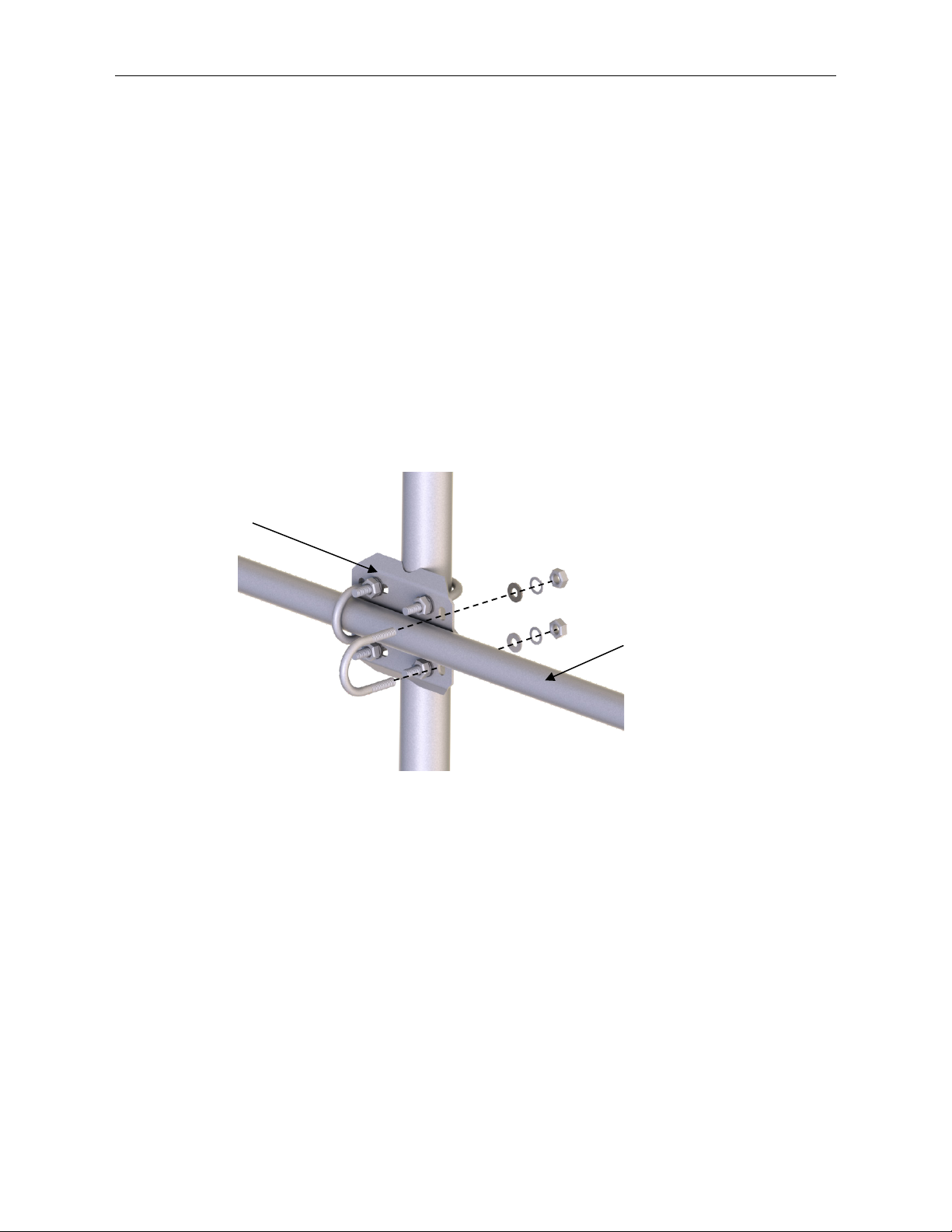
Crossarm-to-Pole
Bracket
CM20X Crossarm
4.1 Hardware Connections
CSAT3B Three-Dimensional Sonic Anemometer
The CSAT3B ships with:
• CM250 leveling mounting kit
• USB data cable
• Certificate of conformance
This QuickStart section covers only the very basic steps in setting up a
CSAT3B using SDM or CPI communications with a Campbell Scientific data
logger. It is intended primarily as an overview and general reference for setup
of a CSAT3B, and is not intended as a replacement for the more detailed
information on installation found in Section 7, Installation
1. Mount a 3.33 cm (1.31 in) outer diameter pipe or crossarm (such as a
CM20X) to a tripod mast or tower as shown in FIGURE 4-1.
(p. 22).
FIGURE 4-1. Mounting a CM20X crossarm with crossarm-to-pole
bracket
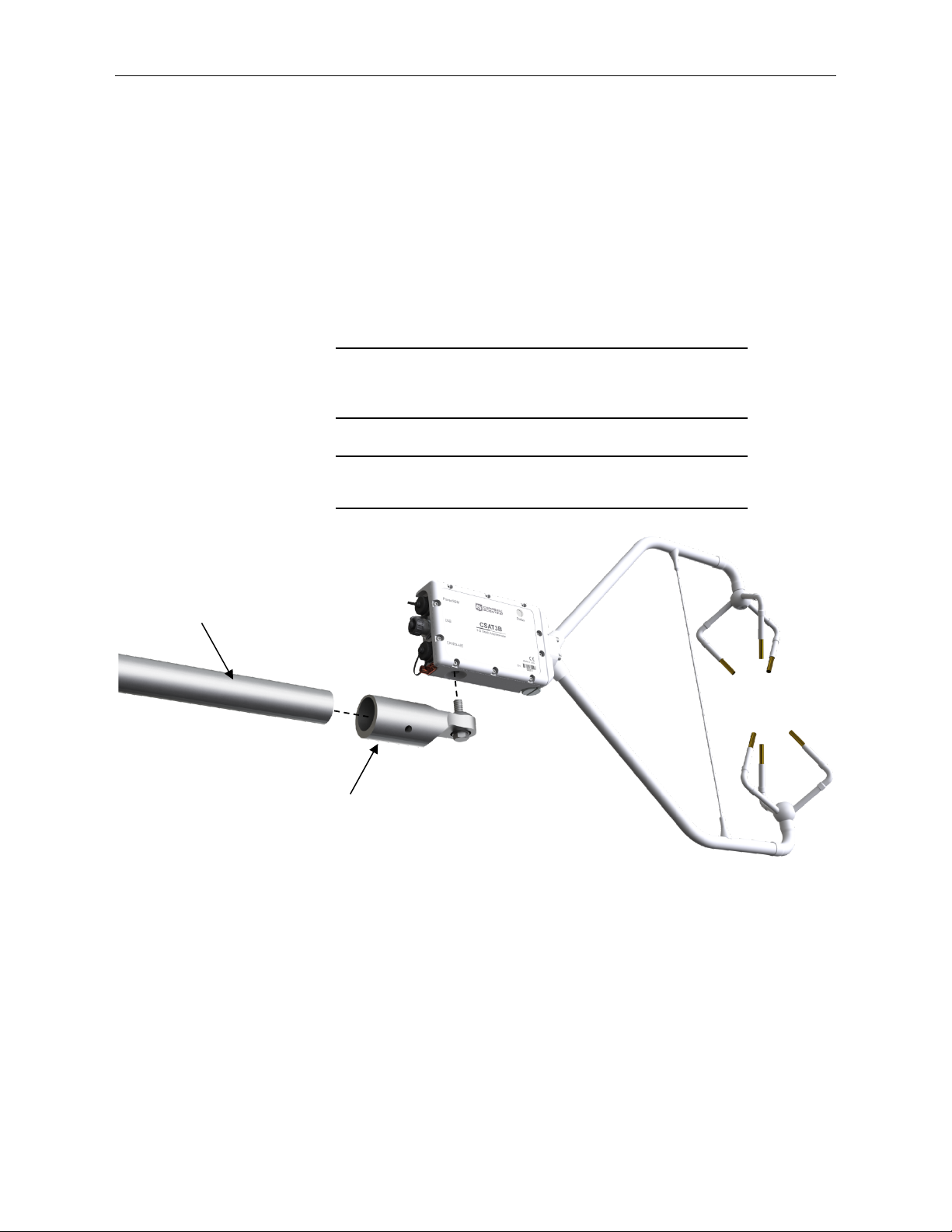
2. Mount the CM250 leveling mount to the end of the crossarm as shown in
FIGURE 4-2.
3. Use the captive bolt on the CM250 to mount the CSAT3B (FIGURE 4-2).
The orientation of the CSAT3B should be level and pointing in the
direction of the prevailing wind.
2
Page 8

CSAT3B Three-Dimensional Sonic Anemometer
NOTE
CM20X Crossarm
CM250 Leveling Mount
CSAT3B Grounding Lug
FIGURE 4-2. CSAT3B mounting
4. Ground the CSAT3B to the tower by attaching a user-supplied, heavy-
gauge wire from the copper grounding lug on the back of the CSAT3B
block (FIGURE 4-3).
5. Earth (chassis) ground the other end of the wire to the CSAT3B mounting
structure or to a grounding rod. For more details on grounding, see the
grounding section of the CR3000 data logger manual.
If connecting multiple CSAT3Bs together either in a series or a
star topology, each CSAT3B must be separately grounded to
either the mounting structure or a grounding rod.
FIGURE 4-3. Grounding lug of CSAT3B
3
Page 9
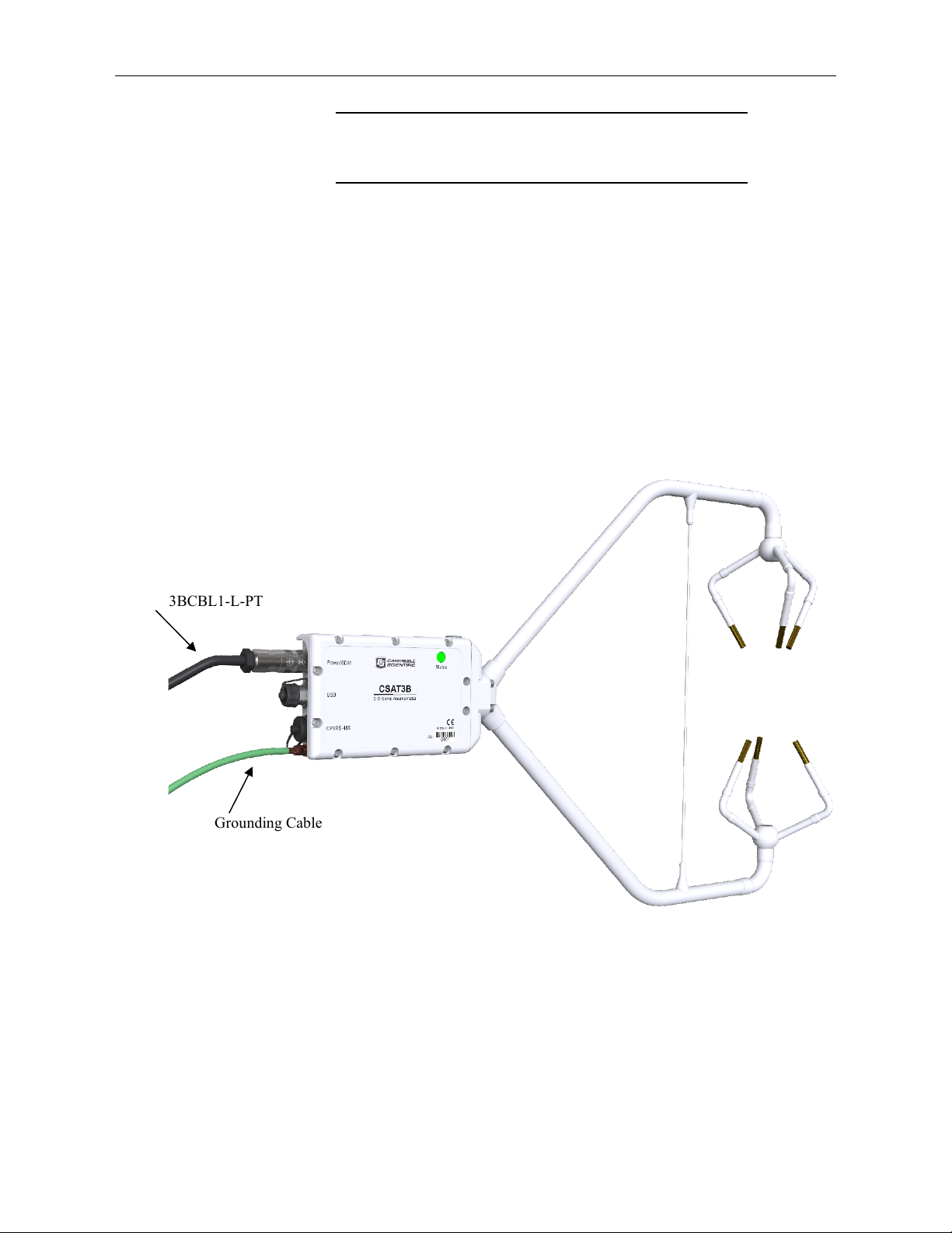
CSAT3B Three-Dimensional Sonic Anemometer
CAUTION
CSAT3BCBL1-L-PT
Grounding Cable
Grounding the CSAT3B is critical. Proper grounding to Earth
(chassis) will ensure maximum ESD protection and improve
measurement accuracy.
4.2 Communications Connections
1. Connect power and communication cable(s).
SDM Communications
If using SDM communications, connect a CSAT3BCBL1-L (“L” denotes
the cable length in feet) cable to the connector on the back of the CSAT3B
block labeled Power/SDM as shown in FIGURE 4-4.
CPI Communications
If using CPI communications connect a CSAT3BCBL2-L cable and a
CSAT3BCBL3-L-RJ to the connectors on the back of the CSAT3B block
labelled Power/SDM and CPI/RS-485, respectively as shown in FIGURE
4-5.
FIGURE 4-4. Cable connection for SDM
4
Page 10

CSAT3B Three-Dimensional Sonic Anemometer
TABLE 4-1. Wiring Diagram for CSAT3B with SDM
CSAT3BCBL2-L-PT
CSAT3BCBL3-L-RJ
Grounding Cable
FIGURE 4-5. Cable connections for CPI
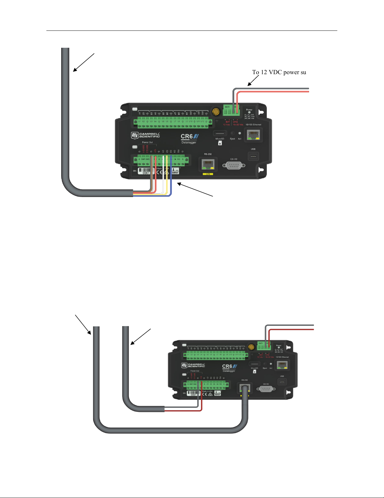
2. Connect power and communication cable(s) to data logger.
SDM Communications
If using SDM communications, connect the wires on the end of the
CSAT3BCBL1-L cable to the data logger SDM and power ports according
to TABLE 4-1. Refer to FIGURE 4-6 which shows these connections to a
CR6 data logger.
Communications
Data Logger Terminal Wire Color
12 V (or other 9.5 to 32 VDC source) Red
Ground Black
Ground Brown
SDM C1 White
SDM C2 Yellow
SDM C3 Blue
Ground Clear
5
Page 11
CSAT3B Three-Dimensional Sonic Anemometer
CSAT3BCBL1 SDM/Power cable from CSAT3B
Wire to power and SDM ports
To 12 VDC power supply
CSAT3BCBL3-L-RJ
CSAT3BCBL2-L-PT
To power supply
FIGURE 4-6. SDM and power wiring to a CR6 data logger
CPI Communications
With CPI communications, connect the red and black wires on the end of
the CSAT3BCBL2-L-PT to the 12 V and ground terminals of a data logger
or to a 9.5 to 32 VDC power supply. Connect the RJ-45 connector on the
end of the CSAT3BCBL3-L-RJ to the CPI port on the CPI-compatible
data logger. Use FIGURE 4-7 as a reference.
FIGURE 4-7. CPI and power connections to a CR6 data logger
6
Page 12

CSAT3B Three-Dimensional Sonic Anemometer
NOTE
3. Use LoggerNet, PC400, or PC200W to send a data logger program to the
data logger. See Section 8.4, Data Logger Programming using SDM or
(p. 57), for more information on data logger instructions and
CPI
programming.
4. Verify that measurements are being made by ensuring the green Status
light (FIGURE 4-8) on the CSAT3B block is blinking, indicating that
measurements are being made and recorded in the data logger without
diagnostic error conditions.
In the default operating Mode 0, where the CSAT3B measurement
and output are triggered by a data logger (see Section 8.2,
Operating Modes
(p. 50), for more details), the CSAT3B Status
light will flash red until a data logger is connected to the CSAT3B
and its program is running and sending measurement triggers.
FIGURE 4-8. Lit status light on CSAT3B block
4.3 Factory Settings
The CSAT3B is shipped from the factory with the default settings that are
shown in TABLE 4-2. These settings can be changed with a computer running
Campbell Scientific Device Configuration Utility, version 2.10 or newer, and
the USB cable that shipped with the CSAT3B. Device Configuration Utility is
available from the Campbell Scientific website in the Support | Downloads
section and is included with LoggerNet, PC400, and PC200W and software
packages.
7
Page 13

CSAT3B Three-Dimensional Sonic Anemometer
TABLE 4-2. CSAT3B Factory Settings
Setting Default
SDM address 3
CPI address 30
Communication
Settings
Measurement
Setting
CPI/RS-485 Communication Port Protocol CPI Enabled
5. Overview
CPI Baud Rate Auto
RS-485 Baud Rate 115200
Unprompted Output Port Disabled
Unprompted Output Rate 10 Hz
Operating Mode
The CSAT3B is an ultrasonic anemometer for measuring sonic temperature
and wind speed in three dimensions. It is often used for studies of turbulence
and flux measurement, where turbulent fluctuations of wind speed and sonic
temperature must be measured at high frequencies; at 10Hz, for example.
From the turbulent wind fluctuations, momentum flux can be calculated. The
covariance of vertical wind and sonic temperature yields sonic sensible heat
flux. By finding the covariance between vertical wind and scalar measurements
made by other fast-response sensors, such as fine-wire thermocouples or gas
analyzers, other fluxes can be calculated. For example, sensible and latent-heat
fluxes, carbon-dioxide flux, and other trace-gas fluxes, can all be measured by
combining the CSAT3B with other sensors.
Mode 0: Data Logger Trigger/No Filter/
Data Logger Prompted Output
5.1 Features
The CSAT3B can communicate measurements using SDM (Synchronous
Device for Measurements), USB, RS-485, and CPI (CAN Peripheral Interface)
communications. For optimal synchronization with other fast-response sensors
for applications such as eddy covariance, Campbell Scientific recommends
using SDM or CPI communications with an appropriate Campbell Scientific
data logger.
The CSAT3B offers the following key features:
• Integrated electronics provide easy mounting of a single piece of
hardware
• Integrated inclinometer
• High-precision measurements ideal for turbulence and eddy
covariance studies
• An improved design with a thin, aerodynamic support strut close to
the ends of the sensor arms, creating greater rigidity and improved
accuracy of sonic temperature
• Supports data logger sampling at any frequency between 1 and 100 Hz
8
Page 14

• New CPI communications for more robust, higher bandwidth
measurements
• Multiple communication options including SDM, CPI, USB, and RS-
485
• Internal temperature and humidity measurements with easily replaced
desiccant
• Version 5 algorithm for calculating data outputs; combines the signal
sensitivity of version 3 with the rain performance of version 4
• Includes options to filter high frequencies for applications requiring
analysis of non-aliased spectra
5.2 Sensor Components
The CSAT3B consists of several components. Some components come
standard with every CSAT3B; others are considered accessories that must be
ordered separately. Some common accessories such as cables are required to
operate a CSAT3B.
5.2.1 Standard Components
Standard components are items that are included or shipped with the CSAT3B.
The following sections describe these items.
CSAT3B Three-Dimensional Sonic Anemometer
5.2.1.1 CM250 Leveling Mounting Kit
The CM250 leveling mounting kit is shipped with the CSAT3B and comes
with an adapter (FIGURE 5-1) that facilitates mounting a CSAT3B at the end
of a 3.33 cm (1.31 in) OD crossarm or pipe. The kit includes a captive 3/8-in
bolt that screws into the bottom of the CSAT3B block, and a 3/16-in Allen
wrench to tighten the adapter on the pipe.
FIGURE 5-1. CM250 mount
5.2.1.2 USB Data Cable
The USB data cable is a 5 m (16 ft) USB cable included with the CSAT3B.
One end has a standard type-A male connector to connect to a computer, while
the opposite end has a mini-B male connector, which connects to the USB port
on the back of the CSAT3B block. The mini-B male connector is rated to
Ingress Protection 68 (IP68) to exclude fine dust and water. When connected
with the cable, Device Configuration Utility allows the user to view or set
settings, send a new operating system to the CSAT3B, or view real-time
measurements. It is also possible to use this cable to collect data with a
computer in unprompted USB mode. Section 6.2, Communications
provides additional information.
(p. 20),
9
Page 15
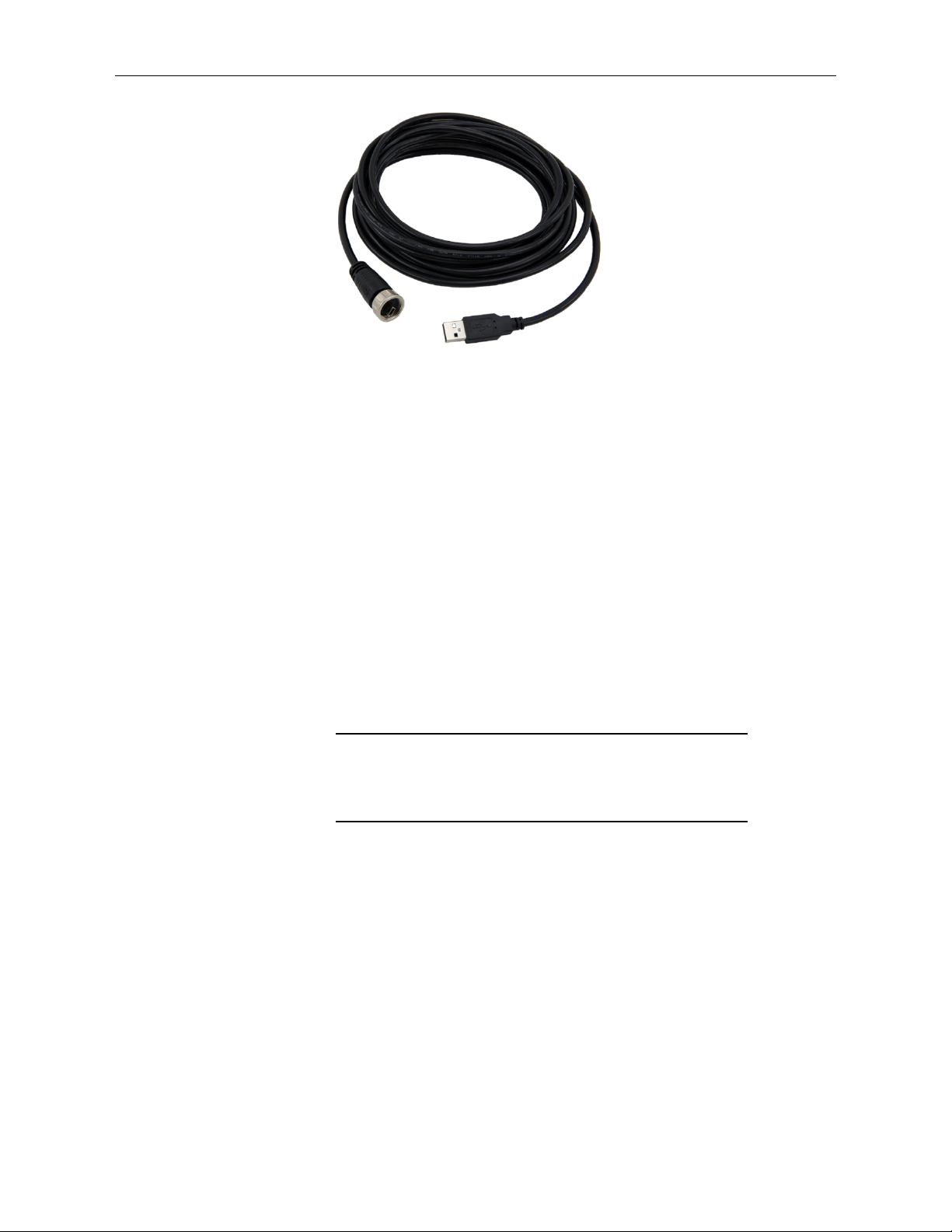
FIGURE 5-2. USB data cable
NOTE
5.2.2 Optional Components
5.2.2.1 Sonic Environment Option
If the CSAT3B is intended to be located in harsh environments such as marine
or heavily fertilized locations, coated transducers, which help prevent
corrosion, can be purchased as an option.
CSAT3B Three-Dimensional Sonic Anemometer
5.2.2.2 Sonic Carrying Case
A large, hard plastic Pelican™ carrying case is available for the CSAT3B. It is
watertight and highly durable. This case is recommended for transporting and
storing the CSAT3B. It includes a set of foam inserts that hold the CSAT3B in
a protected position while providing space for additional components.
If opting out of the sonic carrying case, the CSAT3B will be shipped in a large
cardboard box. The same set of foam inserts used in the sonic carrying case is
used in the cardboard box to securely hold the CSAT3B.
If choosing the cardboard box for shipping, it is recommended to
keep the foam inserts and box. When returning a CSAT3B for
factory recalibration or repair, it is important to ship the unit with
the foam inserts provided from the factory.
5.2.3 Common Accessories
Common accessories for the CSAT3B include cables as well as other
equipment to make sensible heat flux measurements. A fine-wire thermocouple
is an example of an additional sensor often used with a CSAT3B. Descriptions
of cables and other common accessories are described in greater detail in the
following sections.
5.2.3.1 Power and Communications Cables
Cables required for the CSAT3B to be functional, must be ordered along with
the CSAT3B. The types of cables needed for a specific communications mode,
are outlined below.
10
Page 16

CSAT3B Three-Dimensional Sonic Anemometer
NOTE
NOTE
NOTE
Unlike the earlier CSAT3, default-length cables are not included.
This allows the user to specify the exact length, communication
type, and connector type of the cable(s) needed for the application.
Campbell Scientific uses a system for naming cables that provide specific
information about details of the cable and some information about the use of
the cable.
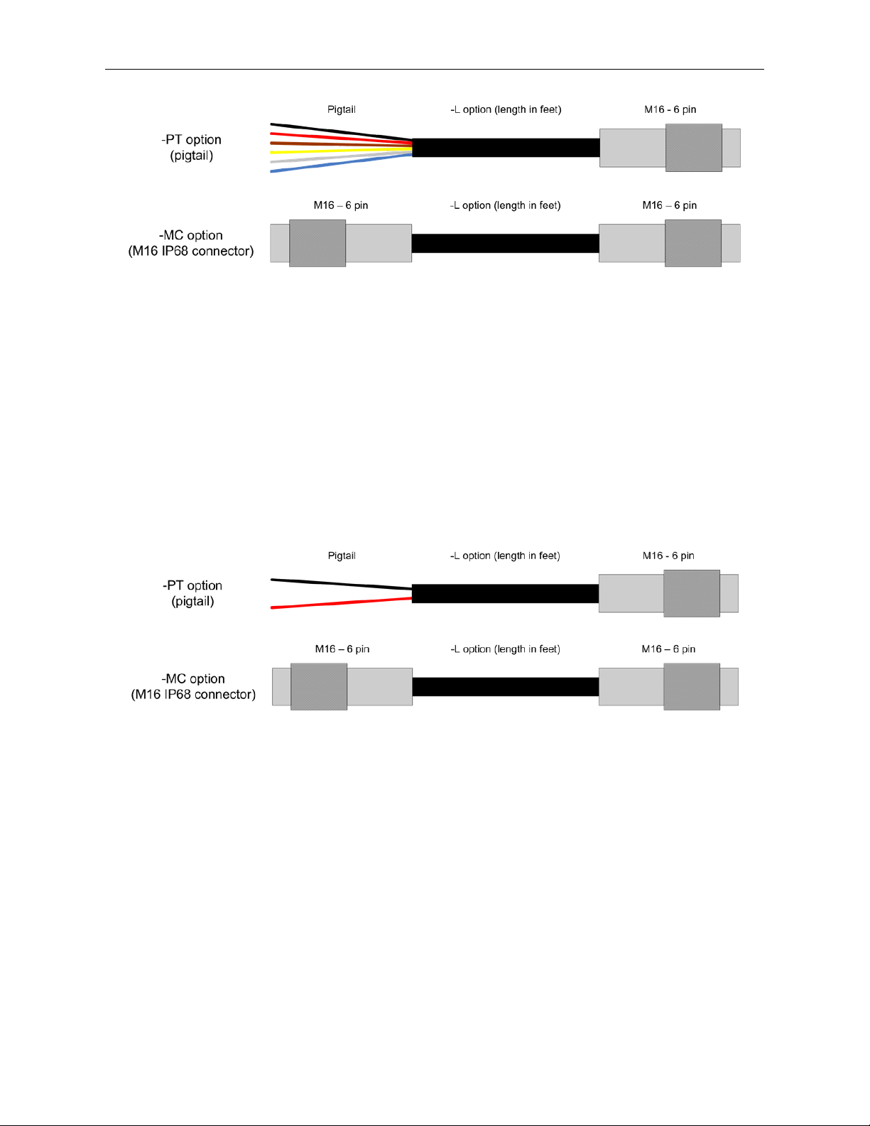
• The ‘–L’ in the cable model name is an option that denotes a user-
specified length of cable in feet.
• The ‘–PT’ is a cable option that specifies one end of the cable to have
pigtail wires for wiring to a power source, data logger terminals, or a
wiring bus. The other end has an M16 connector for connecting to the
corresponding port at the back of the CSAT3B block.
• The ‘–MC’ option designates an M16 connector on both ends of the
cable and is used to daisy-chain several CSAT3B instruments together
in series.
Daisy chaining requires ordering the 30293 splitter (see Section
5.2.4.1, Power/SDM Splitter (p. 15), and Section 5.2.4.2, CPI/RS-
485 Splitter
(p. 15)) for each CSAT3B in series, except the terminal
one.
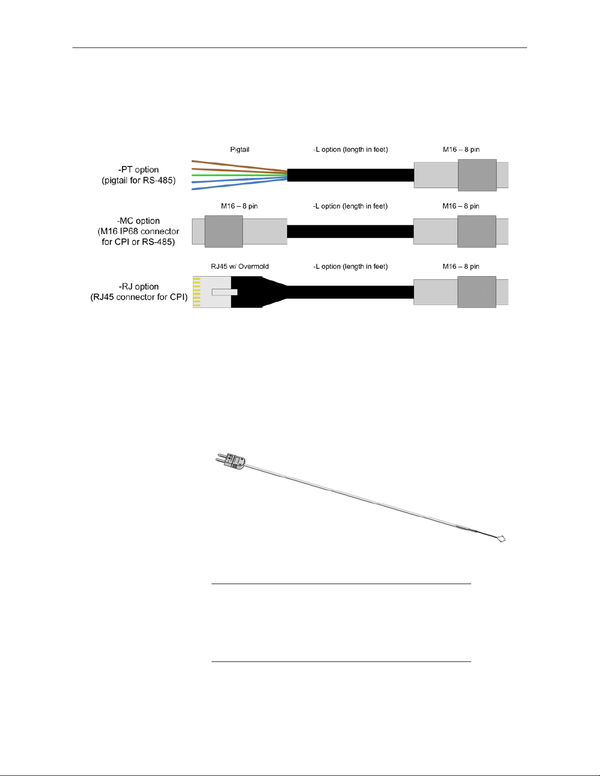
• The ‘–RJ’ option has an RJ-45 connector on one end for connecting
directly to the CPI port on a data logger such as the CR6 or to a CPI
port on the HUB-CPI if a network of several CPI devices are being
installed in a star topology. The other end of the cable has an M16
connector for connecting to the CSAT3B block. The types of cables
needed for a specific communications mode are outlined below. For
information on maximum cable lengths, refer to the communications
specifications in Section 6.2, Communications
(p. 20).
Power/SDM Cable (CSAT3BCBL1)
To use SDM communications to collect data from a CSAT3B with a data
logger, the CSAT3BCBL1-L-PT or CSAT3BCBL1-L-MC should be ordered.
FIGURE 5-3 shows the two versions. This cable transmits both power and
SDM communication signals.
To collect data through another means (CPI, RS-485, USB), the
CSAT3BCBL1 Power/SDM cable may still be used to provide
power to the CSAT3B, in which case the SDM wires should be
left unwired to any ports on the data logger.
11
Page 17
CSAT3B Three-Dimensional Sonic Anemometer
FIGURE 5-3. Options for CSAT3BCBL1 Power/SDM cable
Power Cable (CSAT3BCBL2)
To use CPI, RS-485, or USB communications to collect data from a CSAT3B,
the CSAT3BCBL2-L-PT or CSAT3BCBL2-L-MC should be ordered to
provide power to the sensor. A second cable to transmit the communications is
also required (for example, CSAT3BCBL3 CPI/RS-485 cable for CPI or
RS-485, or the 30179 USB data cable).
For installations with long cable lengths, the CSAT3BCBL2 is preferred over
the CSAT3BCBL1 for providing power due to the heavier gauge wires that
reduce voltage drop over long distances. Allowed length is 1 to 550 ft.
Although the maximum cable length is 550 feet, users requiring a cable length
of 401 to 550 feet should use a 24 V power supply.
FIGURE 5-4. Options for CSAT3BCBL2 power cable
12
Page 18
CSAT3B Three-Dimensional Sonic Anemometer
NOTE
CPI/RS-485 Cable (CSAT3BCBL3)
To use CPI or RS-485 communications to collect data from a CSAT3B, the
CSAT3BCBL3-L-PT, CSAT3BCBL3-L-RJ, or CSAT3BCBL3-L-MC, should
be ordered in addition to a cable to provide power to the sensor (for example,
either the CSAT3BCBL1 or CSAT3CBL2).
FIGURE 5-5. Options for cabling CPI or RS-485 communications
5.2.3.2 FW05 Thermocouple
The FW05 is a Type E thermocouple with a 0.0127 mm (0.0005 in) diameter
(FIGURE 5-6). The thermocouple measures atmospheric temperature
fluctuations and may be used with the CSAT3B to directly calculate sensible
heat flux. Larger size fine-wire thermocouples, such as the FW1 and FW3,
which are more robust but have slower response times, may also be used with
the CSAT3B.
FIGURE 5-6. FW05 thermocouple
Users requiring fine-wire thermocouples for atmospheric
temperature measurements should consider their data logger
choice. The CR6 data logger is not optimal for taking fine-wire
thermocouple measurements. For help in choosing the best data
logger when fine-wire thermocouples are required, contact
Campbell Scientific.
13
Page 19

5.2.3.3 FWC-L Cable
NOTE
The FWC-L is a cable with connector that mates with the connector on a
FW05, FW1, or FW3 fine-wire thermocouple. The other end of the cable has
pigtail wires to wire to a pair of differential voltage terminals on a data logger.
The –L denotes the length of cable in feet, which can be designated at the time
of ordering.
5.2.3.4 Thermocouple Cover
The TC cover is a white metal, thermocouple cover that is placed over the
connectors of the FW05 and the FWC-L cable. It is used to mount the
connectors to the side of the CSAT3B block. It also minimizes temperature
gradients across the connectors.
5.2.3.5 Thermocouple Cover Backplate
The CSAT3B fine-wire thermocouple cover backplate attaches to the CSAT3B
block and is used to cover the back side of the thermocouple (TC) cover.
The backplate is required for the CSAT3B but not for other
Campbell sonic anemometers. In the case of previous models, the
back side of the TC cover is covered by the sensor block.
CSAT3B Three-Dimensional Sonic Anemometer
5.2.3.6 FW/ENC Thermocouple Enclosure
The FW/ENC is a small case (FIGURE 5-7) that is used for storing up to four
fine-wire thermocouples. Due to the fragile nature of the FW05 thermocouple,
it should always be stored in an FW/ENC when not in use. It is also
recommended to order, at a minimum, a set of four FW05 thermocouples for
every CSAT3B as the FW05 will break during normal wear and tear in the
field.
FIGURE 5-7. FW/ENC for storing fragile thermocouples
5.2.4 Other Accessories
The other accessories available for the CSAT3B are used when combining
multiple CSAT3B units into a network of sensors, the data from which are
collected by a single data logger. Networks of CSAT3Bs using SDM or CPI
communications may be configured in one of three different configurations:
• In a series, using a daisy-chain topology
• In parallel, using a star topology
• In a combination of daisy-chain and star topology
14
Page 20
When designing an SDM or CPI network, careful attention should be given not
to exceed a total network cable length that will excessively attenuate the sensor
signals. The exact total length will depend on factors such as sample rate and
topology, but in general the maximum cable lengths (given in Section 6.2,
Communications
followed.
Because CPI communications can support longer network cable lengths, it is
generally recommended as the communication method for sensor networks.
For more detailed information on network topologies and limits on cable
lengths for CPI networks, see the white paper titled Designing Physical
Network Layouts for the CPI Bus, available at www.campbellsci.com.
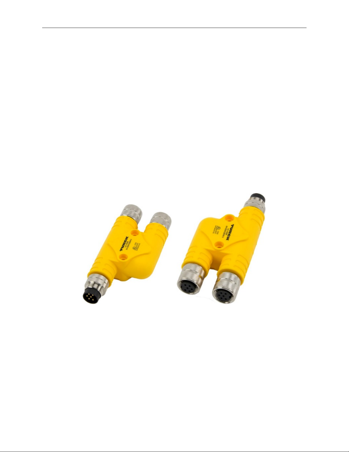
5.2.4.1 Power/SDM Splitter
The Power/SDM splitter has three 6-pin M16 connectors. The splitter, shown
in FIGURE 5-8, allows connection at the Power/SDM port on the back of the
CSAT3B block to two CSAT3BCBL1 or CSAT3BCBL2 cables. The splitter is
IP68 rated, meaning it is dust and watertight. It is used for daisy-chaining
multiple CSAT3Bs in series. A Power/SDM Splitter is required for each
CSAT3B in the daisy chain (regardless of communication method used) except
for the terminal one.
CSAT3B Three-Dimensional Sonic Anemometer
(p. 20)) for each communication type and data rate should be
FIGURE 5-8. CSAT3B Power/SDM splitter (showing pin configuration)
5.2.4.2 CPI/RS-485 Splitter
The CPI/RS-485 splitter has three 8-pin M16 connectors. The splitter allows
connection at the CPI/RS-485 port on the back of the CSAT3B block to two
CSAT3BCBL3 cables. The splitter is IP68 rated. It is used for daisy-chaining
multiple CSAT3Bs in series that use CPI or RS-485 communications. A splitter
is required for each CSAT3B in the daisy-chain, except for the terminal one.
For a daisy-chain of CSAT3Bs using SDM communications, the CPI/RS-485
splitter is not needed. Only the Power/SDM splitter (see Section 5.2.4.1,
Power/SDM Splitter
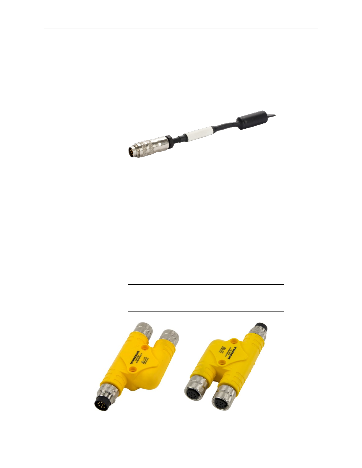
Transient voltage drop is commonly caused by the large series inductance
introduced by either long power cables, multiple CSAT3Bs connected by
(p. 15)) is needed.
15
Page 21
CSAT3B Three-Dimensional Sonic Anemometer
NOTE
splitters, or a combination of both. Because the measurements are
synchronized, multiple CSAT3Bs connected to the same power cable each
draw a pulse of current at the same moment. This has a cumulative effect on
the voltage drop. If the voltage drop is sufficiently large, then the low-voltage
detection circuit inside the CSAT3B sensor can be tripped which forces the
device to reset. A power cable compensation plug for the CSAT3B (FIGURE
5-9) is needed if voltage drop creates problems. The plug is compatible with all
CSAT3Bs. The plug should be placed on the final Power/SDM splitter in the
CSAT3B daisy-chain, farthest from the power supply.
FIGURE 5-9. CSAT3B power cable compensation plug
The primary indicator of low voltage is in the diagnostic flags returned by the
CSAT3B to the data logger. Flag number 32 (0x0020) indicates a low-voltage
condition was detected. If the instrument returns flag 32, first measure the
power source voltage and ensure that its DC value meets specifications. If that
value is appropriate, the voltage at the far end of the cable should be checked.
This must be tested under load so a splitter at the end of the cable will be
required to measure the terminal voltage. These two tests will eliminate the DC
voltage as the source of the problem. Any DC voltage below 12 V at the sensor
would be suspect for susceptibility to droop. In larger systems, even DC
voltages of 13-15 V can still experience enough droop to trigger the detection
under the right conditions. Power systems of 24 V are very unlikely to
experience enough droop to observe this problem. If the DC case checks out
but the flag is still observed, then the system would probably benefit from the
addition of a power compensation plug (FIGURE 5-9).
Both splitters, the CPI/RS-485 and the Power/SDM, look similar;
however, they have a different number of pins and are not
interchangeable.
FIGURE 5-10. CSAT3B CPI/RS-485 splitter (showing pin configuration)
16
Page 22

5.2.4.3 HUB-SDM8
CSAT3B Three-Dimensional Sonic Anemometer
The HUB-SDM8 (shown in FIGURE 5-11) allows up to six SDM devices
(typically, one data logger and multiple SDM sensors) to be connected together
in parallel. In the case of the CSAT3B, up to five CSAT3Bs, or CSAT3B
daisy-chains using CSAT3BCBL1 cables, may be connected to the HUBSDM8. In cases where multiple CSAT3Bs are installed some distance from the
data logger, the HUB-SDM8 can be placed near the CSAT3Bs with a single
SDM cable extended from the hub to the data logger. This decreases the total
network cable length, which limits signal attenuation.
The HUB-SDM8 has eight terminal strips and features spring-loaded guillotine
terminals for easy wiring. It comes in a watertight enclosure and includes a Ubolt for mounting to a vertical pipe or mast. An SDM Cable (CABLE5CBL-L;
see Section 5.2.4.4, SDM Cable CABLE5CBL-L
(p. 17)) should be ordered to
connect the HUB-SDM8 to a data logger and a power supply.
FIGURE 5-11. HUB-SDM8 for multiple CSAT3B connections with SDM
communications
5.2.4.4 SDM Cable CABLE5CBL-L
The SDM cable, CABLE5CBL-L, is a 22 AWG, five-conductor cable with a
Santoprene jacket and an aluminum Mylar shield. By default, the conductors
are stripped and tinned.
The CABLE5CBL-L is used to connect the power and SDM connection from a
HUB-SDM8 to the power and SDM connections on a power source and data
logger.
5.2.4.5 HUB-CPI
The 8-channel RJ45 HUB-CPI allows up to eight CPI devices to be connected
together in parallel. In the case of the CSAT3B, up to seven CSAT3Bs, or
CSAT3B daisy-chains using CSAT3BCBL3 cables, may be connected in
parallel to the HUB-CPI. The remaining port may be used with a CAT5e or
CAT6 Ethernet cable (see Section 5.2.4.4, SDM Cable CABLE5CBL-L
connect the HUB-CPI to the CPI port on a data logger such as the CR6.
(p. 17)) to
17
Page 23

CSAT3B Three-Dimensional Sonic Anemometer
The HUB-CPI (shown in FIGURE 5-12) is not weatherproof and should be
housed in an enclosure, typically alongside the data logger.
FIGURE 5-12. HUB-CPI for multiple CSAT3B connections to CPI
communications
5.2.4.6 CAT6 Ethernet Cable
The CAT6 Ethernet cable is a 61 cm (2 ft), unshielded CAT6 network cable
with RJ45 connectors. Typically, it connects the HUB-CPI to the CPI port on a
data logger such as the CR6.
FIGURE 5-13. CAT6 Ethernet cable
6. Specifications
The CSAT3B measures wind speed and the speed of sound along the three
non-orthogonal sonic axes. The wind speeds are then transformed into the
orthogonal wind components u
, uy, and uz, and are referenced to the
x
18
Page 24

CSAT3B Three-Dimensional Sonic Anemometer
anemometer head. The reported ultrasonic air temperature (T
between the temperatures computed for the three non-orthogonal sonic axes.
The vector component of the wind that is normal to each sonic axis (such as a
crosswind) leads to a measurement error that is corrected online by the
CSAT3B before the wind speed is transformed into orthogonal coordinates.
Because of this correction, it is not necessary to apply the speed of sound
correction described by Liu et al., 2001 (see Section 10.1, References
The CSAT3B has several operating modes to suit different applications. The
anemometer can be configured to make a single measurement per data logger
trigger, or it can operate in a self-triggered mode. When self-triggering, the
CSAT3B will make measurements at a high rate, apply an optional userselectable bandwidth filter, and provide the latest output upon receiving an
output prompt. An output prompt may come from the data logger, or in the
case of unprompted output mode (such as computer data collection), the output
is prompted by the CSAT3B itself. The default operating mode of the CSAT3B
is to make measurements when triggered by a data logger (SDM or CPI),
which does not apply any low-pass (high-cut) filtering. See Section 4.2,
Communications Connections
Section 8.2, Operating Modes
6.1 Measurements
Operating Temperature
Standard: –30 to 50 °C
Wind Accuracy (–40 to 50 °C, wind speed < 30 m·s
Offset Error
: ± 8 cm·s
u
x
: ± 8 cm·s–1 max
u
y
: ± 4 cm·s–1 max
u
z
Gain Error
Wind Vector ± 5° of horizontal: ± 2% of reading max
Wind Vector ± 10° of horizontal: ± 3% of reading max
Wind Vector ± 20° of horizontal: ± 6% of reading max
Wind Resolution
: 1.0 mm·s–1 RMS
u
x
: 1.0 mm·s–1 RMS
u
y
: 0.5 mm·s–1 RMS
u
z
Wind Full Scale Range: ± 65 m·s
Sonic Temperature Resolution: ± 0.002 °C RMS at 25 °C
Sonic Temperature Reporting Range: –30 to 50 °C
Measurement Rates
Data Logger Triggered: 1–100 Hz
Unprompted Output (to computer): 10, 20, 50, or 100 Hz
Internal Self-Trigger Rate: 100 Hz
) is the average
s
(p. 68)).
(p. 4), for a list of all default settings, and see
(p. 50), for more information on modes.
–1
, azimuth angles between ± 170 °C)
–1
max
–1
19
Page 25

Measurement Delay
Data Logger Triggered (no filter): 1 trigger period (1 scan interval)
Unprompted Output (no filter): 10 ms
Filtered Output (Data Logger Prompted or Unprompted to computer):
795 ms with 5 Hz bandwidth filter
395 ms with 10 Hz bandwidth filter
155 ms with 25 Hz bandwidth filter
Filter Bandwidths: 5, 10, or 25 Hz
Internal Monitor Measurements
Update Rate: 2 Hz
Inclinometer Accuracy: ± 1 °
Relative Humidity Accuracy: ± 3% over 10 − 90% range
± 7% over 0 − 10% range
± 7% over 90 − 100% range
Board Temperature Accuracy: ± 2 °C
6.2 Communications
SDM: Used for data logger based data acquisition.
Bit Period: 10 µs to 1 ms
Cable Length: 7.6 m (25 ft) max @ 10 µs bit period
76 m (250 ft) max @ 1 ms bit period
Address Range: 1 – 14
Bus Clocks per Sample: ~200
CPI: Used for data logger based data acquisition.
Baud Rate: 50 kbps to 1 Mbps
Cable Length:
122 m (400 ft) max @ 250 kbps
853 m (2800 ft) max @ 50 kbps
Address Range: 1 – 120
Bus Clocks per Sample: ~300
RS-485: Used for anemometer configuration or computer-based data acquisition.
Baud Rate: 9.6 kbps to 115.2 kbps
Cable Length: 305 m (1000 ft) max @ 115.2 kbps
610 m (2000 ft) max @ 9.6 kbps
Bus Clocks per Sample: ~500 (ASCII formatted)
USB: Used for anemometer configuration or computer-based data acquisition.
Connection Speed: USB 2.0 full speed 12 Mbps
Cable Length: 5 m max
i
15 m (50 ft) max @ 1 Mbps
CSAT3B Three-Dimensional Sonic Anemometer
i
For additional details, refer to CSI whitepaper “Designing Physical Network Layouts for the CPI
Bus”
20
Page 26

6.3 Power Requirements
Voltage Requirement: 9.5 – 32 VDC
Current Requirement (10 Hz Measurement Rate)
Current @ 12 VDC: 110 mA
Current @ 24 VDC: 65 mA
Current Requirement (100 Hz Measurement Rate)
Current @ 12 VDC: 145 mA
Current @ 24 VDC: 80 mA
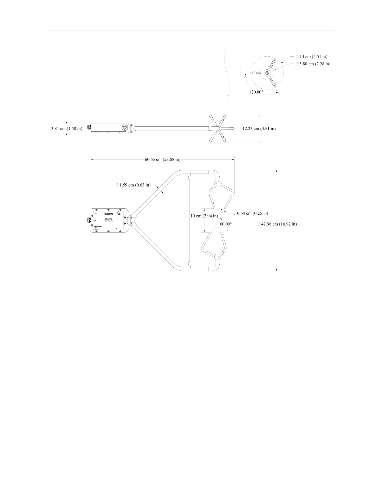
6.4 Physical Description
Dimensions
Anemometer Overall: 60.7 cm (23.9 in) length
43.0 cm (16.9 in) height
12.2 cm (4.8 in) width
Measurement Path: 10.0 cm (3.9 in) vertical
5.8 cm (2.3 in) horizontal
Transducer Angle: 60 degrees from horizontal
Transducer Diameter: 0.64 cm (0.25 in)
Transducer Mounting Diameter: 0.84 cm (0.33 in)
Support Arm Diameter: 1.59 cm (0.63 in)
Cardboard Box with Foam: 73.7 x 45.7 x 25.4 cm (29 x 18 x 10 in)
Carrying Case with Foam: 79.5 x 51.8 x 31 cm (31.3 x 20.4 x 12.2 in)
Weight
Anemometer Head: 1.45 kg (3.2 lb)
Including Cardboard Box Option: 5.3 kg (11.7 lb)
Including Carrying Case Option: 13.4 kg (29.5 lb)
Shipping (Both cardboard and carrying cases options are shipped within a second box)
Cardboard Box Option
Weight: 9.1 kg (20.0 lb)
Dimensions: 91 x 51 x 41 cm (36 x 20 x 16 in)
Carrying Case Option
Weight: 16.3 (36.0 lb)
Dimensions: 81 x 66 x 43 cm (32 x 26 x 17 in)
CSAT3B Three-Dimensional Sonic Anemometer
21
Page 27
CSAT3B Three-Dimensional Sonic Anemometer
7. Installation
FIGURE 6-1. Dimensions of CSAT3B
Campbell Scientific recommends that the CSAT3B and data acquisition system
is setup in a laboratory setting before field installation. This provides an
opportunity to verify that settings and programs are correct in a controlled
environment. Prior to setup, the user needs to know information about the
desired sensor settings, orienting, mounting, and leveling the CSAT3B, which
is covered in the following sections.
If the CSAT3B is to be used in a marine environment, or in an environment
where it is exposed to corrosive chemicals (for example, the sulfur-containing
compounds in viticulture), attempt to mount the CSAT3B in a way that reduces
the exposure of the sonic transducers to saltwater or corrosive chemicals. In
marine or viticulture environments, the sonic transducers are expected to age
more quickly and require replacement sooner than a unit deployed in an inland,
chemical-free environment.
22
Page 28

7.1 Settings
CSAT3B Three-Dimensional Sonic Anemometer
Prior to installation, the CSAT3B settings should be verified. This is done by
the following steps:
1. Provide power to the CSAT3B by connecting the M16 connector of
either a CSAT3BCBL1 or CSAT3BCBL2 to the Power/SDM port on
the back of the CSAT3B block. The other end of this cable will have
red and black wires that should be connected to a 9.5 to 32 VDC
power source. (In the case of the CSAT3BCBL1, the other wires need
not be connected.)
2. Connect the circular connector on the USB data cable included with
the CSAT3B to the port labelled USB on the back of the CSAT3B
block. Connect the other end of the cable to a USB port on a
computer.
3. Launch Device Configuration Utility (downloaded from
www.campbellsci.com).
4. From the left side of the main screen, select the CSAT3B among the
list of sensors. Select the appropriate communication port and baud
rate (refer to the left side of FIGURE 7-1).
5. If this is the first time the computer has connected to a CSAT3B and
depending on the computer settings, the USB driver may need to be
manually installed. To do this, make sure the computer is connected to
the internet and click on the install the USB driver link as shown in
FIGURE 7-1).
6. Once the driver has been installed, if needed, press the Connect
button at the bottom left of the window.
23
Page 29

CSAT3B Three-Dimensional Sonic Anemometer
TABLE 7-1. CSAT3B Settings and Status Values in Device Configuration Utility
Shows real-time measurements of Ux, Uy, Uz,
Setting or Status
Subscreen
Real-Time Data
Value Options Description
Anemometer
Data
FIGURE 7-1. Connecting CSAT3B using Device Configuration Utility
7. Once connected, the main screen will have a section with tabs to view
the following four subscreens: Real-Time Data, Communication
Settings, Measurement Settings, and Instrument ID. TABLE 7-1
describes each of the settings or status values in these subscreens. For
each setting or status value, the factory default setting is noted by the
footnote. Ensure that the appropriate settings are enabled for the
communication protocol that will be used. An example subscreen is
shown in FIGURE 7-2.
sonic temperature (Ts), and the diagnostic
word. If operating in Mode 0 (see Section
Operating Modes
-
second. The Status light on the CSAT3B will
(p. 50)), values will flash each
8.2,
also flash red if in Mode 0 when no
measurement triggers are being received from
a data logger (for example, if a data logger is
not connected to the CSAT3B).
24
Page 30

TABLE 7-1. CSAT3B Settings and Status Values in Device Configuration Utility
Subscreen
Internal
1 through 120
10 Hz1/
CSAT3B Three-Dimensional Sonic Anemometer
Setting or Status
Value Options Description
Communication
Settings
Temperature
Internal Relative
Humidity
Inclinometer
Pitch
Inclinometer Roll -
SDM Address
CPI Address
Communication
Port Protocol
1 through 14
3
301/
Disable Both
CPI Enabled
RS-485 Enabled
Auto
1000 kbps
CPI Baud Rate
500 kbps
250 kbps
125 kbps
50 kbps
1200
2400
4800
RS-485 Baud
Rate
9600
19200
38400
57600
115200
230400
Unprompted
Output Port
Disabled
USB Port
RS-485 Port
- Temperature inside CSAT3B block
Relative humidity inside CSAT3B block.
-
-
Change desiccant if greater than 50% (see
Section 9.3, Desiccant
(p. 62)).
Pitch angle of CSAT3B head (see Section 7.3,
Mounting
(p. 29))
Roll angle of CSAT3B head (see Section 7.3,
Mounting
1/
Unique address for SDM device
(p. 29))
Unique address for CPI device
Identifies whether the RS-485/CPI port will be
1/
disabled, enabled for CPI, or enabled for
RS-485
1/
Baud rate for CPI communications
(in most circumstances this setting should
remain set to Auto)
Baud rate for RS-485 communications
1/
1/
Identifies the port to output unprompted data
Unprompted
Output Rate
20 Hz
50 Hz
100 Hz
Identifies the rate at which to output
unprompted data
25
Page 31

TABLE 7-1. CSAT3B Settings and Status Values in Device Configuration Utility
Subscreen
Mode 0: Data logger
A unique identifier in addition to the serial
NOTE
NOTE
Measurement
Settings
Instrument ID
CSAT3B Three-Dimensional Sonic Anemometer
Setting or Status
Value Options Description
triggered | No filter |
Data logger
1/
prompted output
Mode 1: Self
Operating Mode
triggered | Filtered |
Data logger
prompted output
Mode 2: Self
triggered | No filter |
Unprompted output
Identifies the source of the measurement
trigger, whether a low pass filter will be
applied, and the output mode (see Section 8.2,
Operating Modes
(p. 50), for more details on
operating mode)
to computer
Mode 3: Self
triggered | Filtered |
Unprompted output
to computer
5 Hz
Filter Bandwidth
10 Hz
25 Hz
Sonic Transducer
Shadow
Correction
Anemometer
Serial Number
Disabled
Enabled
Serial Number
User ID String Blank1/
Factory ID String Blank1/
OS Version -
The cut-off frequency of the low pass filter.
Only applicable if in Operating Mode 1 or 3.
Applies an optional Kaimal correction for
wind shadowing of the sonic transducers. See
Section 8.1.3, Sonic Transducer Shadow
Correction
1/
The serial number of the CSAT3B
(p. 49).
A unique identifier in addition to the serial
number that the user may assign
number that the factory may assign
The version number of the CSAT3B operating
system
OS Date - The date the loaded operating system was built
1/
Denotes a factory default setting
Factory defaults for all setting may be restored by clicking the
Factory Defaults button at the bottom of the screen in the Device
Configuration Utility.
The SDM communications port is always enabled.
26
Page 32
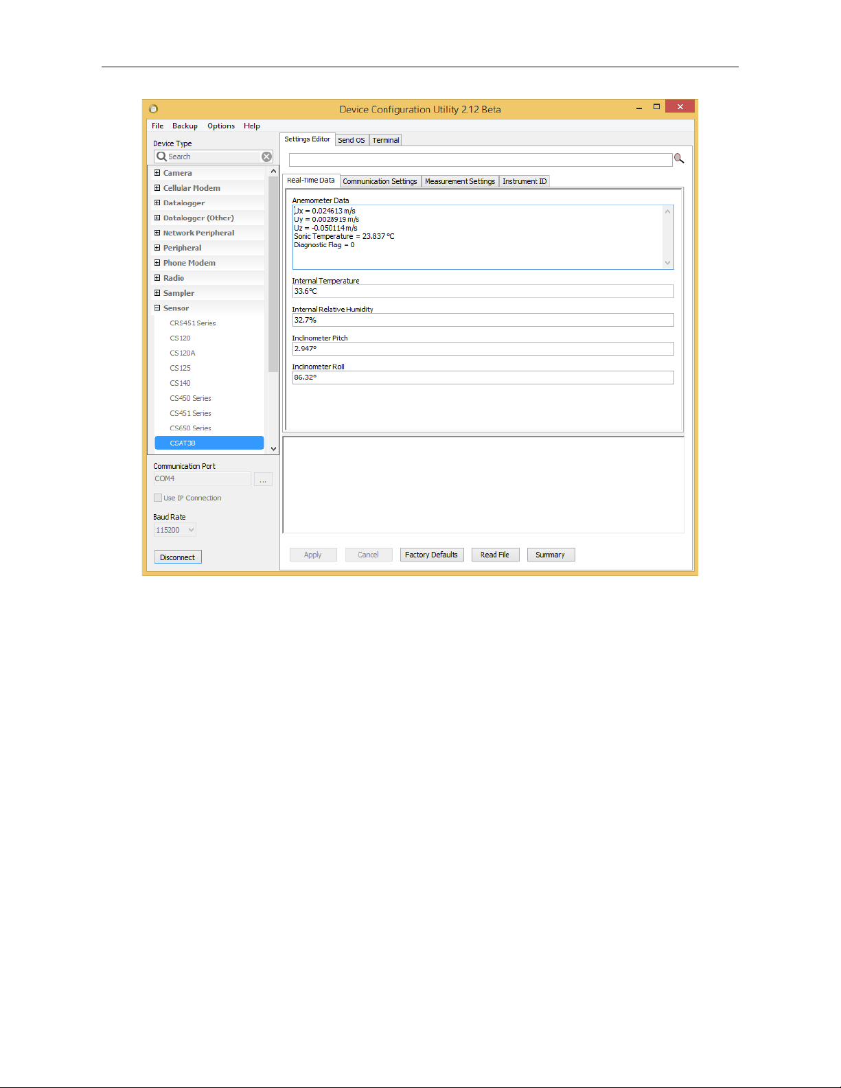
CSAT3B Three-Dimensional Sonic Anemometer
FIGURE 7-2. Real-time data subscreen while connected to CSAT3B
7.2 Orientation
The three components of wind are defined by a right-handed orthogonal
coordinate system. The CSAT3B points into the negative x direction (see
FIGURE 7-7). If the anemometer is pointing into the wind, it will report a
positive u
In general, the anemometer should be pointed into the prevailing wind to
minimize interference from support structures such as the tower or tripod.
Typically, the anemometer should be mounted level to the ground as described
in Section 7.4, Leveling
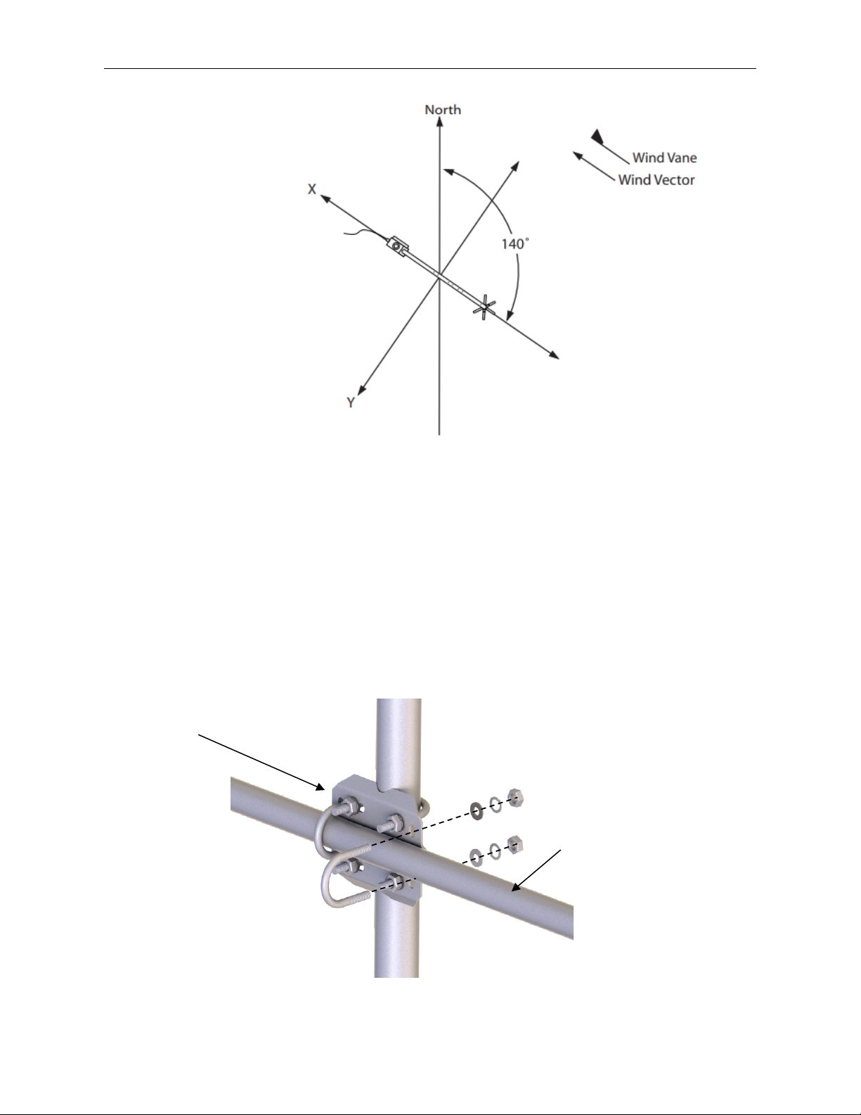
7.2.1 Sonic Azimuth
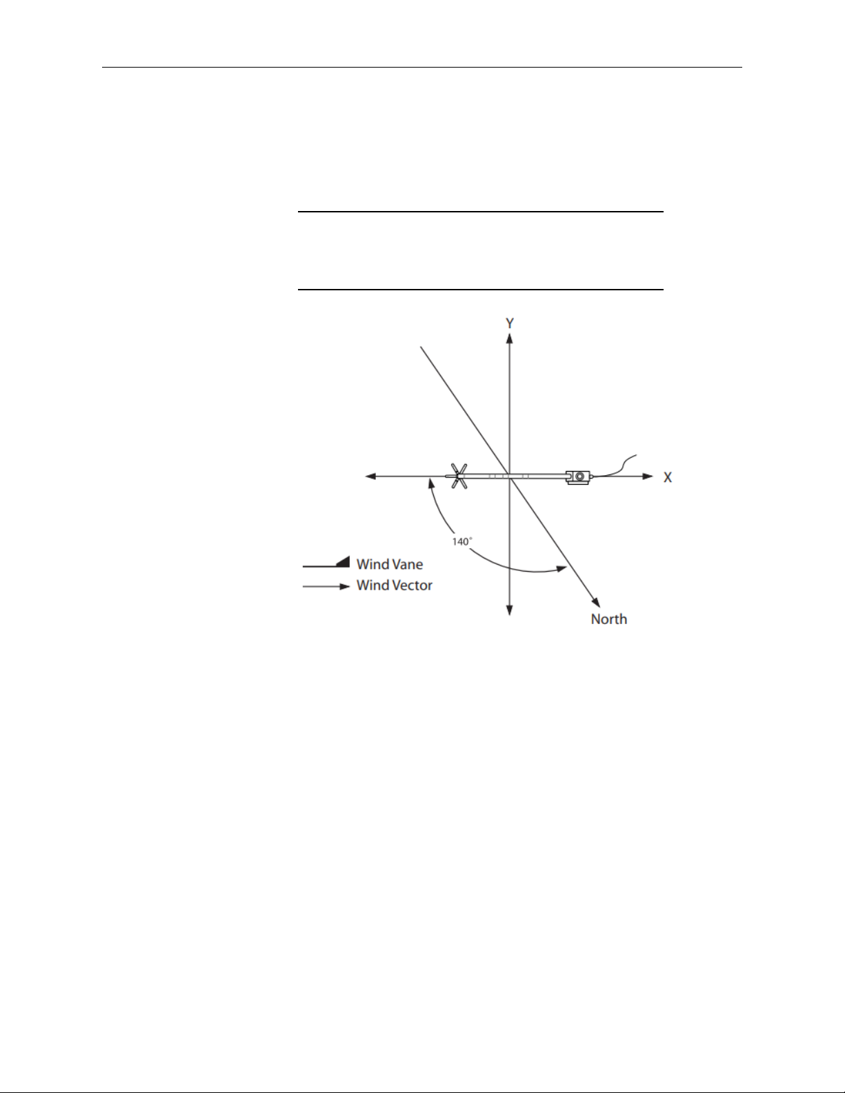
The example programs report the wind direction in both the sonic coordinate
system (a right-handed coordinate system; FIGURE 7-3) and in the compass
coordinate system (a left-handed coordinate system; FIGURE 7-4). The sonic
coordinate system is relative to the sonic itself and does not depend on the
sonic orientation (azimuth of the negative x-axis). The compass coordinate
system is fixed to Earth. For the program to compute the correct compass wind
direction, the azimuth of the sonic negative x-axis must be entered into the
with Device Configuration Utility
wind.
x
(p. 30).
27
Page 33
CSAT3B Three-Dimensional Sonic Anemometer
NOTE
program. The program default value for the variable CSAT_AZIMUTH is 0.
This assumes that the prevailing wind is from the north (e.g., the sonic is
mounted such that the negative x-axis points to the north). To change this to the
appropriate azimuth, open the CRBasic program and navigate to Const
CSAT_AZIMUTH and input the correct azimuth and send this updated
program to the data logger.
Remember to account for the magnetic declination at the site; see
Appendix A, CSAT3B Orientation (p. A-1), for details. If using an
app on a cellular phone, magnetic declination is most likely
already taken into consideration.
FIGURE 7-3. Right-hand coordinate system, horizontal wind vector
angle is 0 degrees
28
Page 34
CSAT3B Three-Dimensional Sonic Anemometer
CM210 Mounting Kit
CM20X Crossarm
FIGURE 7-4. Compass coordinate system, compass wind direction is
140 degrees
7.3 Mounting
The CSAT3B is supplied with mounting hardware to attach it to the end of a
horizontal pipe with an outer diameter of 3.33 cm (1.31 in), such as the
Campbell Scientific CM202, CM204, or CM206 crossarm (referred to
generically as a CM20X crossarm). The following steps describe the normal
mounting procedure.
1. Secure the chosen crossarm to a tripod or other vertical structure using
a CM210 crossarm-to-pole mounting kit as shown in FIGURE 7-5.
FIGURE 7-5. CM210 mounting kit with CM20X crossarm
29
Page 35
CSAT3B Three-Dimensional Sonic Anemometer
CAUTION
CAUTION
CM20X Crossarm
CM250 Leveling Mount
2. Point the horizontal arm into the direction of the prevailing wind and
tighten the nuts and bolts of the mounting hardware.
3. Attach the CM250 leveling mount (included with the CSAT3B) to the
crossarm by tightening the set screws on the boom adapter with a
3/16-in hex socket head wrench. Refer to FIGURE 7-6.
4. Attach the CSAT3B to the leveling mount by inserting the bolt on the
mount into the threaded hole on the bottom of the CSAT3B block as
shown in FIGURE 7-6.
5. Lightly tighten the bolt and then proceed to the leveling steps.
Do not carry the CSAT3B by the arms or the strut between
the arms. Always hold the CSAT3B by the block, where the
upper and lower arms connect.
Over-tightening bolts will damage the screw threads in the
CSAT3B block.
FIGURE 7-6. CSAT3B mounting
7.4 Leveling
Leveling the CSAT3B within a couple degrees is usually sufficient. The user
commonly applies coordinate rotations to time-series data to report the threedimensional wind in a coordinate system where the x- and y-axis lie along the
stream-wise wind plane.
Adjust the anemometer head so that the bubble within the level on top of the
CSAT3B block is in the bullseye. Firmly grasp the sonic anemometer block,
loosen the bolt underneath the block, and adjust the head accordingly. Finally,
tighten the bolt with a 9/16-in wrench.
30
Page 36

CSAT3B Three-Dimensional Sonic Anemometer
If an application requires greater accuracy in inclination of the CSAT3B, or if
an application requires a measurement that shows if, and when, the inclination
of the CSAT3B changes over time (for example, a sagging crossarm or tower
tilt), an integrated inclinometer in the CSAT3B can give pitch and roll
measurements.
Pitch is the angle between the gravitationally horizontal plane and the CSAT3B
x-axis. A positive pitch angle corresponds to a clock-wise rotation about the yaxis when looking down on the y-axis (see FIGURE 7-7). In other words, a
positive pitch angle occurs when the transducer end of the CSAT3B is pointed
downwards, while a negative pitch angle occurs when CSAT3B is pointed
upwards.
Roll is the angle between the gravitationally horizontal plane and the CSAT3B
y-axis. A positive roll angle corresponds to a counter-clockwise rotation about
the x-axis when looking down the x-axis (see FIGURE 7-7).
The inclinometer is sampled at a rate of 2 Hz and is not necessarily
synchronized with the wind and sonic temperature data outputs. For
applications that require correction for a moving measurement platform (on a
buoy or ship, for example), a separate fast-response inclinometer, gyrometer,
and accelerometer sensor should be used and sampled at the same rate as the
CSAT3B wind measurements.
The outputs of the CSAT3B integrated inclinometer can be viewed by
connecting the USB data cable to the CSAT3B and a computer running
Campbell Scientific Device Configuration Utility. It can also be output using
the CRBasic instruction CSAT3BMonitor. See Section 8.4.1.2,
CSAT3BMonitor()
(p. 58), for more information about setting this instruction.
31
Page 37

CSAT3B Three-Dimensional Sonic Anemometer
x y z
roll
pitch
FIGURE 7-7. CSAT3B shown with coordinate system, with arrows
representing positive x, y, and z axes; curved arrows indicate
positive rotations of pitch and roll angles
7.5 Additional Fast-response Sensors
7.5.1 Fine-Wire Thermocouple
A fine-wire thermocouple (model FW05 with a FWC-L cable, TC cover, and
TC cover backplate) can be mounted to the side of the anemometer block to
measure temperature fluctuations.
First, attach the thermocouple (TC) cover backplate to the CSAT3B with the
screw that was included. Next, attach the female connector from the FWC-L to
the side of the anemometer with the short screw (#2-56 x 0.437 inch) that was
provided with the white thermocouple cover. Insert the male connector of the
FW05 into the female connector of the FWC-L. Finally, attach the
thermocouple cover to the anemometer block using the thumb screw so that
both the FW05 and FWC-L connectors are covered. See FIGURE 7-8 for
positioning and FIGURE 7-9 with the FW05 fully installed.
32
Page 38

CSAT3B Three-Dimensional Sonic Anemometer
TC Cover Backplate
TC Cover
FWC-L
FW05
FIGURE 7-8. Exploded view of fine-wire thermocouple (TC) with
CSAT3B
FIGURE 7-9. CSAT3B with fine-wire thermocouple mounted
33
Page 39

7.5.2 Other Gas Analyzers
NOTE
If a fast-response gas analyzer is being used with the CSAT3B, care should be
taken to mount the analyzer (open-path) or the analyzer intake (closed-path) as
close as possible to the sonic sampling volume in order to obtain good spatial
and temporal synchronicity between vertical wind and gas concentration
fluctuations while also retaining adequate spatial separation. This will avoid
excessive wind distortion. In general, mount the analyzer or its intake
downwind of the sonic sampling volume.
7.6 Wiring
On the back of the CSAT3B block there is a copper grounding lug (refer to
FIGURE 4-3). Use a standard flat-head screwdriver to pinch an 8 AWG to
14 AWG wire between the lug and the lug screw. Campbell Scientific offers a
10 AWG copper wire that is suitable for grounding sensors. Connect the other
end of the wire to the tripod or tower, which should be grounded to Earth.
The CSAT3B has three watertight circular ports or connectors at the rear of the
block. These are labeled Power/SDM, USB, and CPI/RS-485 as shown in
FIGURE 4-3. Unless a port is in use and connected to a cable, they should be
securely covered by one of the caps that are captive to the CSAT3B.
CSAT3B Three-Dimensional Sonic Anemometer
The appropriate port and cable type to be used are determined by the chosen
communication method. TABLE 7-2 shows some of the criteria to use when
determining the best communication method for a given application. Once a
suitable method is determined, the appropriate combination of cables,
connectors, and lengths should be used (see Section 5.2.3.1, Power and
Communications Cables
(p. 10), for information about ordering cables).
If the CSAT3B is going to be operated using SDM or CPI communications
where the data logger triggers the measurement and the data are unfiltered (see
Mode 0 in Section 8.2, Operating Modes
(p. 50)), then the CSAT3B default
settings are appropriate and do not require modification. If, however, the
CSAT3B will be operated in another mode that either requires data filters or
uses USB or RS-485 communications, the settings must be modifying as
described in Section 7.1, Settings
(p. 23).
Unlike previous CSAT3 models, the CSAT3B does not include
7.6 m (25 ft) lengths of all cable types. Only the 5 m (16 ft) USB
cable for initial configuration of the sensor is included. Other
cables must be ordered separately.
34
Page 40

CSAT3B Three-Dimensional Sonic Anemometer
TABLE 7-2. Summary of Communications Options for the CSAT3B
NOTE
NOTE
SDM USB CPI RS-485
Data collection
Data loggers:
• CR6
• CR800
• CR1000X
• CR3000
Computer
Data loggers:
• CR6
1/
• CR800
• CR1000X
• CR3000
1/
1/
Computer
Cable length Medium Short, < 5 m Longest Long
Required cables CSAT3BCBL1
CSAT3BCBL2 and
USB cable (included)
CSAT3BCBL2 and
CSAT3BCBL3
CSAT3BCBL2 and
CSAT3BCBL3
Robustness Better Worse Best Better
Bandwidth OK Best Best OK
Synchronization
with other sensors
Best Worse Best Worse
Noisy environments OK OK Best Better
1/
Requires using the SC-CPI Interface
CPI communications is preferred over SDM communications
when using a CR6 or CR1000X data logger. See TABLE 7-2 to
examine the suitability of communications type based on various
parameters for other combinations.
7.7 Communications
There are many possible configurations of multiple CSAT3Bs and other
sensors on a single measurement station or system. Accordingly, power
requirements and sensor cable lengths should be taken into account to
appropriately power all sensors and avoid excess attenuation of signals. The
following sections describe different types of communications and different
configurations that may be helpful when designing the layout and configuration
of a system. For additional help, contact Campbell Scientific.
For all communications types, if the total number of CSAT3Bs
and other sensors powered by the data logger exceeds the limit of
output current from the data logger, the power wires must be
connected to a separate 12 to 32 VDC power supply. For long
cables, a higher voltage power supply is recommended as there
will be voltage loss over long distances.
35
Page 41

CSAT3B Three-Dimensional Sonic Anemometer
NOTE
WARNING
For CSAT3B sensor networks with relatively long cables, the
inductive impedance can be great enough to lead to short dips in
voltage. If the voltage drops below 9.5 VDC at the input of any
CSAT3B sensor, that sensor will report a Low Voltage diagnostic
bit (see
TABLE 8-6) and the Status light will flash red. To resolve
this issue, power the CSAT3B network using a higher voltage (up
to 32 VDC) or install a capacitor at one of the current loads. If
needed, contact Campbell Scientific for assistance.
Not all of the data loggers that are compatible with the
CSAT3B support the same voltage input range as the
CSAT3B. While the CSAT3B supports voltage of up to
32 VDC, many data loggers require lower voltage. For
example, the CR800 and CR3000 require 9.6 to 16 VDC
when connecting to the front panel voltage input, the
CR1000X requires 10 to 18 VDC.
If a CR3000 has a rechargeable base, then a 17 to
28 VDC power supply may be connected to the base.
Unlike most of the data loggers, the CR6 does support
up to 32 VDC if the power supply is connected to the
CHG input terminals. For more details, refer to a data
logger user manual.
7.7.1 SDM Communications
If data collection from the anemometer is to be accomplished using a data
logger with SDM communications, connect a CSAT3BCBL1 to the
Power/SDM port by screwing in the M16 connector into the port until tight as
shown in FIGURE 7-10. No other cables are required for SDM
communications, as the CSAT3BCBL1 contains both power and SDM wiring.
If only one CSAT3B is being measured, the opposite end of the cable will have
wire pigtails if connecting directly to the ports on a data logger. Refer to
Section 4.2, Communications Connections
white, yellow, and blue wires to the SDM-C1, SDM-C2, and SDM-C3 ports
respectively, on a data logger (FIGURE 7-11). On a data logger or another 9.5
to 32 VDC power supply, connect the red and black wires to the 12 V and G
ports, respectively. See FIGURE 7-11 and TABLE 7-3 for wiring and wire
color designations.
For applications requiring very long cable lengths, a higher voltage power
supply is recommended as voltage drop over long distances will occur and the
CSAT3B requires a minimum of 9.5 VDC.
(p. 4), for this wiring. Connect the
36
Page 42

CSAT3B Three-Dimensional Sonic Anemometer
CSAT3BCBL1-L-PT
Grounding Cable
CSAT3BCBL1 SDM/Power cable from CSAT3B
Wire to power and SDM ports
To 12 VDC power supply
FIGURE 7-10. SDM/Power connections
FIGURE 7-11. Wiring to power and SDM ports on CR6 data logger
For an application that requires SDM communications from multiple
CSAT3Bs in series, or with a daisy-chain topology, first connect to each
CSAT3B as described in Section 7.1, Settings
(p. 23), to ensure each sensor has
been assigned a unique SDM address. Connect a CSAT3BCBL1 to the
Power/SDM port of the terminal CSAT3B. The opposite end will have an M16
connector that mates with one of the split M16 connectors on the Power/SDM
37
Page 43

CSAT3B Three-Dimensional Sonic Anemometer
splitters. Next, screw the side of the splitter with only one M16 connector to
the Power/SDM port of the second CSAT3B. Connect another CSAT3BCBL1
to the splitter and down to the next CSAT3B. Continue the daisy chain until the
last CSAT3B. The final CSAT3BCBL1 should have pigtail wire ends to
connect to the SDM and 12 V ports of a data logger. See FIGURE 7-12.
If several CSAT3Bs using SDM communications are being connected in
parallel or with a star topology, connect a CSAT3BCBL1 cable to the
Power/SDM port of each CSAT3B, and connect the other wires on the pigtail
end of the cables to a HUB-SDM8 bus (see Section 5.2.4.3, HUB-SDM8
(p. 17)).
Connect the wires so that all wires of a common color or signal are on the same
rail. Then, use a CABLE5CBL with pigtail wires to connect the HUB-SDM to
the SDM and 12 V ports of a data logger. See FIGURE 7-13.
38
Page 44

CSAT3B Three-Dimensional Sonic Anemometer
CSAT3BCBL1-L-MC
CSAT3BCBL1-L-MC
CSAT3BCBL1-L-PT
To power supply
To power supply
Power/SDM Splitter
Power/SDM Splitter
FIGURE 7-12. SDM daisy chain (CSAT3B sensor arms and grounding
cables not shown)
39
Page 45

CSAT3B Three-Dimensional Sonic Anemometer
NOTE
To power supply
CSAT3BCBL1-L-PT
CABLE5CBL-L
FIGURE 7-13. SDM star topology (CSAT3B sensor arms and
grounding cables not shown)
7.7.2 CPI Communications
If data collection from the anemometer is to be done by a data logger using CPI
communications, then connect a CSAT3BCBL2 to the Power/SDM port by
screwing in the M16 connector into the port until tight.
A CSAT3BCBL1 may also be used for power, but the SDM wires
will not be used. The CSAT3BCSBL1 also has lighter gauge
power wires, which increases voltage loss over long cable length,
so it should only be used for shorter cable lengths.
Next, connect a CSAT3BCBL3 to the CPI/RS-485 port in the same manner. If
only one CSAT3B is being measured, the opposite end of the power cable
should have pigtail wires which may be wired to the 12 V and G terminals on a
data logger or to another 12 to 32 VDC power supply. The CPI cable should
have the RJ-45 connector plugged into the CPI port of the data logger.
40
Page 46

CSAT3B Three-Dimensional Sonic Anemometer
CSAT3BCBL2-L-PT
CSAT3BCBL3-L-RJ
Grounding Cable
CSAT3BCBL3-L-RJ
CSAT3BCBL2-L-PT
To power supply
FIGURE 7-14. Power and CPI cable connections
FIGURE 7-15. CPI connection to a CR6 data logger
41
Page 47

CSAT3B Three-Dimensional Sonic Anemometer
NOTE
CPI Daisy-chain Topology
For an application that requires CPI communication from multiple CSAT3Bs
in series, or with a daisy-chain topology, first connect to each CSAT3B as
described in Section 7.1, Settings
(p. 23), to give each sensor a unique CPI
address. Then connect a CSAT3BCBL2 to the Power/SDM port and a
CSAT3BCBL3 to the CPI/RS-485 port on the terminal CSAT3B. The opposite
end of the power cable should use an M16 connector to mate with one of the
split M16 connectors on the power/SDM splitter. The opposite end of the CPI
cable should use an M16 connector to mate with one of the split M16
connectors on the CPI/RS-485 splitter.
Screw the side of the splitters with only one M16 connector to the Power/SDM
and CPI/RS-485 ports of the second CSAT3B. Connect another set of cables
from these splitters down to the next CSAT3B. Continue the daisy-chain until
the last CSAT3B, where a final CSAT3BCBL2 should have pigtail wire ends
to connect to the 12 V and G ports of a data logger or to a 12 to 32 VDC power
supply. The final CSAT3BCBL3 should have an RJ-45 connector that plugs
into the CPI port of the data logger. Refer to FIGURE 7-16 for the described
connections.
CPI Star Topology
If several CSAT3Bs using CPI communications are being connected in parallel
or with a star topology, connect a CSAT3BCBL2 cable to each Power/SDM
port of each CSAT3B, and connect the other wires to the 12 V and G ports of a
data logger or to another 12 to 32 VDC power supply (for convenience, it’s
possible to use a wiring bus such as the HUB-SDM8 to bring several power
wires together and then extend a single cable such as the CABLEPCBL-L from
the bus to the power supply).
Connect a CSAT3BCBL3 to each CPI/RS-485 port of each CSAT3B, and
connect the opposite end, which should have RJ-45 connectors to a HUB-CPI.
Then, use a CAT5e or CAT6 Ethernet cable to connect the HUB-CPI to the
CPI port of a data logger. Refer to FIGURE 7-17 for these connections.
The sockets or ports on the HUB-CPI are all the same. It does not
matter which socket is used to connect to the data logger or to
other CSAT3Bs.
42
Page 48
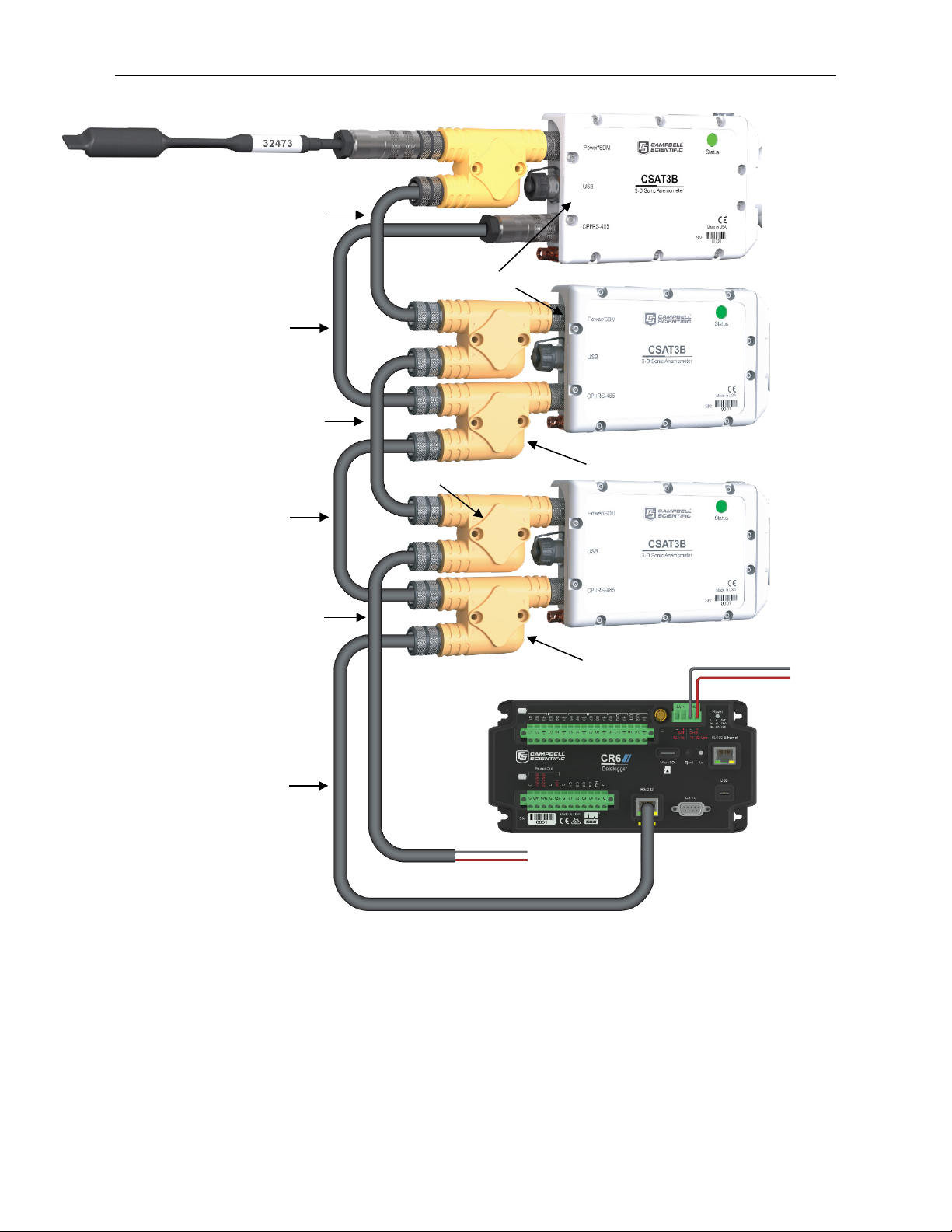
CSAT3B Three-Dimensional Sonic Anemometer
To power supply
To power supply
Power/SDM Splitter
CPI/RS-485 Splitter
CPI/RS-485 Splitter
CSAT3BCBL2-L-MC
CSAT3BCBL3-L-MC
CSAT3BCBL2-L-MC
CSAT3BCBL3-L-MC
CSAT3BCBL2-L-PT
CSAT3BCBL3-L-RJ
Power/SDM Splitter
FIGURE 7-16. CPI daisy chain (CSAT3B sensor arms and grounding
cables not shown)
43
Page 49

CSAT3B Three-Dimensional Sonic Anemometer
HUB-CPI
To power supply
CAT6 Cable
CSAT3BCBL2-L-PT
CSAT3BCBL3-L-RJ
FIGURE 7-17. CPI star topology (CSAT3B sensor arms and grounding
cables not shown)
44
Page 50

7.7.3 RS-485 Communications
NOTE
NOTE
If data collection from the anemometer is to be accomplished by a computer
using RS-485, first connect the CSAT3B as described in Section 7.1, Settings
(p. 23), to confirm the following four settings:
Operating Mode:
• Mode 2: Self triggered | No filter | Unprompted output to
computer, or
• Mode 3: Self triggered | Filtered | Unprompted output to computer
(If Mode 3, select filter bandwidth.)
CPI/RS-485 Communication Port Protocol: RS-485 Enabled
RS-485 Baud Rate: 115200 or other appropriate value
Unprompted Output Port: RS-485 Port
• Unprompted Output Rate: 10, 20, 50 or 100 Hz
In Device Configuration Utility the settings for Unprompted
Output Port and Unprompted Output Rate will be grayed-out
until the operating mode has been set to Mode 2 or Mode 3.
To complete installation, connect a CSAT3BCBL2 to the Power/SDM port by
screwing in the M16 connector into the port until tight.
CSAT3B Three-Dimensional Sonic Anemometer
A CSAT3BCBL1 may also be used for power, but the SDM wires
will not be used. The CSAT3BCSBL1 also has lighter gauge
power wires, which increases voltage losses over long cable
length, so it should only be used for shorter cable lengths.
Next, connect a CSAT3BCBL3 cable to the CPI/RS-485 port in the same
manner. If only one CSAT3B is being measured, the opposite end of the power
cable should have pigtail wires, which may be connected to a 12 to 32 VDC
power supply, and the RS-485 cable should have pigtail wires for wiring to a
connector on a computer (see FIGURE 7-18). Refer to TABLE 7-2 for a
summary of the receive-and-transmit wiring.
45
Page 51

CSAT3B Three-Dimensional Sonic Anemometer
NOTE
NOTE
CSAT3BCBL2-L-PT
CSAT3BCBL3-L-RJ
Grounding Cable
7.7.4 USB
FIGURE 7-18. RS-485 cable connections
If data collection from the anemometer is to be done by a computer using USB
communications, first connect to the CSAT3B as described in Section 7.1,
Settings
(p. 23), to confirm the following three settings:
Operating Mode:
• Mode 2: Self triggered | No filter | Unprompted output to
computer
or
• Mode 3: Self triggered | Filtered | Unprompted output to computer
(If Mode 3, select filter bandwidth.)
Unprompted Output Port: USB Port
Unprompted Output Rate: 10, 20, 50 or 100 Hz
In Device Configuration Utility, the settings for Unprompted
Output Port and Unprompted Output Rate will be grayed-out
until the operating mode has been set to Mode 2 or Mode 3.
To complete installation, connect a CSAT3BCBL2 to the Power/SDM port by
screwing in the M16 connector into the port until tight.
A CSAT3BCBL1 may also be used for power, but the SDM wires
will not be used. The CSAT3BCSBL1 also has lighter gauge
power wires, which increases voltage losses over long cable
length, so it should only be used for shorter cable lengths.
46
Page 52

CSAT3B Three-Dimensional Sonic Anemometer
TABLE 7-3. CSAT3B Cable Wire Assignments
TABLE 7-4. FW05/FWC-L
WARNING
Connect the 5 m (16 ft) USB cable included with the CSAT3B to the USB port
in the same way. If only one CSAT3B is being measured, the opposite end of
the power cable should have pigtail wires, which may be connected to a 12 to
32 VDC power supply, and the USB cable should be connected to a USB port
on a computer.
For a watertight connection to the USB port, use the included USB cable. For a
temporary, non-watertight connection to the USB port, any USB male A type
to male Mini-B type cable can be used.
Unused ports on the CSAT3B block should always have
the caps securely screwed on to avoid water damage to
the electronics.
CSAT3B
Cable Type Signal Description Pigtail Color
Power 9.5-32 VDC Red
Ground Black
SDM GND Brown
CSAT3BCBL1
CSAT3BCBL2
CSAT3BCBL3
If a fine-wire thermocouple such as a model FW05 with FWC-L is being used,
the wiring designations in TABLE 7-4 should be followed to connect the
thermocouple to a differential voltage terminal on a data logger.
SDM C1 White
SDM C2 Yellow
SDM C3 Blue
Shield Clear
Power 9.5-32 VDC Red
Ground Black
RxA Brown
RxB Brown stripe
TxA Blue
TxB Blue stripe
RGND Green
Fine-Wire Thermocouple
Description Color
Signal high Purple
Signal low Red
47
Page 53

8. Operation
8.1 Theory of Operation
CSAT3B Three-Dimensional Sonic Anemometer
The CSAT3B uses three pairs of non-orthogonally oriented transducers that
transmit and receive ultrasonic signals. The time of flight of a sonic signal
between a pair of transducers is directly related to the wind vector component
that is parallel to the sonic axis. The CSAT3B is able to calculate the wind
vector components along each sonic axis using the time difference between an
outgoing and return sonic signal, along with the distance between sonic
transducers. Trigonometric relationships are used to calculate the wind speed in
an orthogonal x-y-z coordinate system.
The time of flight measurement is also related to the speed of sound in air,
which is a function of the air density (temperature and humidity). Through
these relationships, the CSAT3B is able to output a measurement of sonic air
temperature from which actual air temperature may be calculated if humidity is
known.
For more complete details on the theory of operation of the CSAT3B, refer to
Appendix B, CSAT3B Measurement Theory
(p. B-1).
8.1.1 Algorithm Version 5
Since the release of the original CSAT3 in 1996, various improvements have
been made to the algorithms used for signal processing and measurement
output. Each time a significant change has been made to these algorithms, a
new version number has been issued. The CSAT3B uses algorithm Version 5.
Version 5 maintains many of the advantages of signal recognition and
diagnostic sensitivity that were made possible by Version 3, while also adding
the advantages of performance during precipitation events made possible by
Version 4. It also resolves Version 4 issues of speed-of-sound measurement
errors in very high wind conditions as reported by Burns et al., 2012 (see
Section 10.1, References
(p. 68)).
8.1.2 Effects of Crosswind on the Speed of Sound
The speed of sound is found by combining the out and back time-of-flight
measurements (see Equation B-5 in Appendix B, CSAT3B Measurement
Theory
does not affect the measured speed of sound, the perpendicular component
does. An online calculator can account for the effects of the perpendicular
component of wind using the measured components of wind and simple
trigonometry, or manually by using the methods described by Schotanus et al.,
1983 and Liu et al., 2001 (see Section 10.1, References
corrects for the effects of crosswind on the speed of sound.
The equations derived by Schotanus et al., 1983, apply to sonic anemometers
that make speed of sound measurements from a single pair of transducers. Liu
et al. extends these equations to sonic anemometers that measure the speed of
sound on all three axes and then averages the results to a single speed of sound
as with the CSAT3B. Liu et al. assume that the geometry of each individual
three-dimensional anemometer is ideal when they derive the factors given in
Table 1 of their publication.
(p. B-1)). While the parallel component of the wind along the sonic axis
(p. 68)). The CSAT3B
48
Page 54

CSAT3B Three-Dimensional Sonic Anemometer
NOTE
Liu et al., 2001, recommend that CSAT3B sonic temperature
variances and sonic sensible heat flux are corrected for the effects
of cross wind. The CSAT3B, however, performs an online
correction. Additional correction of CSAT3B data for cross-wind
effects will cause errors in the measured fluxes.
8.1.3 Sonic Transducer Shadow Correction
The CSAT3, CSAT3A, and CSAT3B suffer minimal wind distortion compared
to many other sonic anemometer designs because of a very low ratio of
transducer diameter to sonic path length and since the non-orthogonal
geometry keeps the sonic paths at angles closer to perpendicular with respect to
a mean horizontal wind flow. However, there are cases, such as when
oncoming wind has high angles of attack (for example, low frequency eddies
on a tall tower), that will lead to more shadowing. Accordingly, an optional
wind shadow correction specific to the CSAT3-series transducer diameter and
sonic path length has been implemented in the CSAT3B OS versions 1.11 and
newer.
This shadow correction, known as the Kaimal correction (Kaimal, 1979 and
Horst et al, 2015), is applied according to:
= 0.84 + 0.16 (
)
Where:
U
= the magnitude of the wind vector parallel to the sonic path without
i
shadowing errors
i = a placeholder index for
a, b
, or c , representing the three sonic paths,
and
θ
= the angle between the three-dimensional wind vector and the wind
i
vector component along the a-, b-, or c-sonic path (see FIGURE 8-1)
The CSAT3B embedded code improves the estimates of θ – and therefore the
accuracy of the correction – by iteratively applying the above correction three
times for each measurement of each sonic path. Since there continues to be
some debate on the appropriateness of this and other shadow corrections in
turbulent versus laminar flows, the default of this setting is Disabled.
49
Page 55

CSAT3B Three-Dimensional Sonic Anemometer
θa
U
Ua
FIGURE 8-1. Angle θ
oncoming wind, U, and the wind component along the a-sonic path,
.
U
a
8.2 Operating Modes
The CSAT3B has different operating modes that are selected based on the
desired measurement trigger source, presence of a data filter, and type of data
output. Specifically, the following four modes are available:
• Mode 0: Data logger triggered | No filter | Data logger prompted output
• Mode 1: Self triggered | Filtered | Data logger prompted output
• Mode 2: Self triggered | No filter | Unprompted output to computer
• Mode 3: Self triggered | Filtered | Unprompted output to computer
The mode is selected using the Device Configuration Utility under the
Measurement Settings tab (see Section 7.1, Settings
viewing and selecting settings). TABLE 8-1 gives a summary of the CSAT3B
operating modes. The following sections give more information on the
measurement trigger, data filters, and data output as a guide to selecting the
appropriate mode. Mode 0 is the default operating mode for the CSAT3B and
is recommended when fluxes are the primary interest.
is defined as the angle between the vector of
a
(p. 23), for details on
50
Page 56
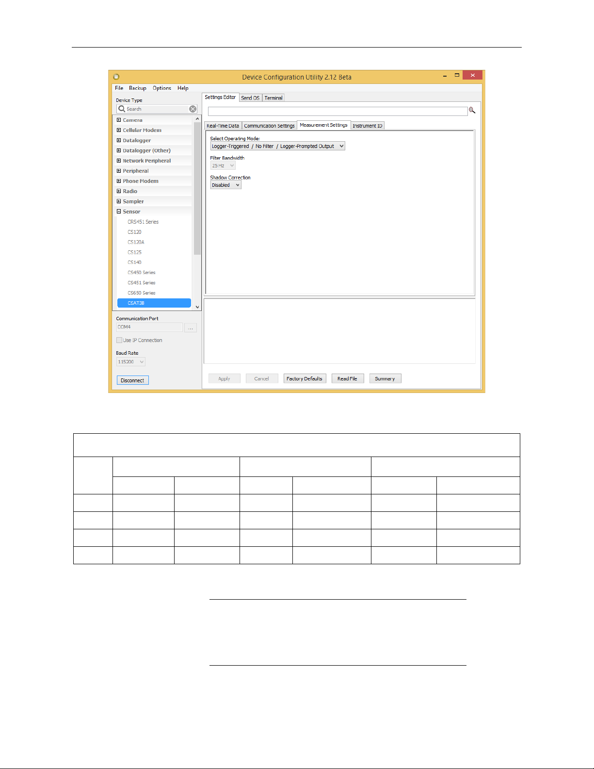
CSAT3B Three-Dimensional Sonic Anemometer
TABLE 8-1. Overview of CSAT3B Operating Modes
NOTE
FIGURE 8-2. Measurement settings in Device Configuration Utility
Measurement Trigger Filters Output Prompt
Mode
Source Rate Enabled Bandwidth (Hz) Source Rate
0 Data logger 1 to 100 Hz1/ No - Data logger 1 to 100 Hz1/
1 CSAT3B 100 Hz Yes 5, 10, 25 Data logger 1 to 100 Hz1/
2 CSAT3B 100 Hz No - CSAT3B 10, 20, 50, 100 Hz
3 CSAT3B 100 Hz Yes 5, 10, 25 CSAT3B 10, 20, 50, 100 Hz
1/
The exact rate is determined by the scan interval set in the CRBasic program of the
data logger.
Data logger prompted output using Mode 0 requires use of SDM
or CPI communications. Data logger prompted output using
Mode 1 requires CPI communications (SDM not compatible with
bandwidth filters). The options for unprompted output to a
computer require use of RS-485 or USB communications.
51
Page 57

8.2.1 Measurement Trigger
NOTE
A measurement trigger is the actual command to initiate a sonic measurement
and can be driven by either a data logger or the CSAT3B internal timer. If the
trigger is given by a data logger as in Mode 0, then no data filtering is done
(bandwidth is wide open) since each trigger will initiate a single new
measurement (single-measurement regime). The data logger can trigger
measurements at rates from 1 to 100 Hz. If the trigger is given by the internal
CSAT3B timer as in Modes 1 ˗ 3, the measurements will be self triggered at a
rate of 100 Hz. This results in an oversampled measurement regime where the
100 Hz samples may be optionally processed through a filter before being
downsampled or decimated and output.
If a data logger fails to provide a trigger and the CSAT3B has not
been configured for unprompted output, the CSAT3B will enter
into a lost-trigger state where it will output measurements at 1 Hz
based on its internal timer. If the CSAT3B is in a lost-trigger state
while connected with Device Configuration Utility, real-time
anemometer data will flash on the screen at one second intervals
and the LED Status light on the CSAT3B head will flash red.
This is an indication that the settings should be checked. It does
not indicate a problem with the CSAT3B hardware. Once a
trigger is received by the CSAT3B, or once unprompted output is
enabled, normal operation will ensue.
CSAT3B Three-Dimensional Sonic Anemometer
8.2.2 Data Filter
The optional data filter (Modes 1 and 3) takes the 100 Hz sample points that
were self triggered by the CSAT3B and runs them through a low-pass (highcut) filter, resulting in a new filtered output at the same 100 Hz rate. The
degree to which the data are filtered is determined by the user-selected filter
bandwidth. This is selected from the Device Configuration Utility in the
Measurement Settings tab.
The bandwidth is the frequency at which a signal is filtered to (1-1/e) of its
original power. In cases where unaliased spectra from the CSAT3B are to be
analyzed, the user should choose a filter bandwidth that is at the Nyquist
frequency, which is half the data output rate from the CSAT3B to the data
logger or computer. This will eliminate aliasing or the mismatch of signals to
frequencies. The bandwidths that are available for selection are 5, 10, and
25 Hz. Each mode and bandwidth results in a different time delay between
measurement and output. TABLE 8-2 summarizes these time delays which will
need to be accounted for when aligning CSAT3B data with data from other
fast-response sensors. Data alignment can be done automatically with a data
logger or during post-processing on a computer. TABLE 8-4 also shows the
closest integer sample delays for various output rates.
If the primary interest of a study is fluxes rather than spectral analysis, there is
no need to select a filter. With unfiltered data, the anemometer high frequency
response is limited only by the geometry of the anemometer head. This
minimizes the possibility of underestimating high-frequency signal variations
and covariations. This approach, however, aliases high-frequency information
to lower frequencies. This aliasing is apparent in spectra from an upwards tail,
when compared to the −5/3 power relationship (Kaimal and Finnigan), at
frequencies approaching the Nyquist frequency of one-half the sample rate.
52
Page 58

CSAT3B Three-Dimensional Sonic Anemometer
Bandwidth
NOTE
NOTE
This aliasing does not compromise the variances and covariances (and
therefore, fluxes) computed from aliased data. The variance and covariance
calculations are not frequency dependent, they simply measure a signal’s total
variation or total covariation from two signals, respectively. Given this, under
circumstances where measuring fluxes are the primary interest, it is
recommended to operate without a filter and, if possible, have the data logger
provide the trigger.
TABLE 8-2. Time Delays by Mode and Filter
Delay between Measurement
Mode
and Output
0 1 Data Logger Scan Interval
2 10 ms
5 Hz 795 ms
8.2.3 Data Output
1 and 3
10 Hz 395 ms
25 Hz 155 ms
Modes 1 and 3 and the associated bandwidth filters were fully
supported starting with CSAT3B OS versions 1.09 and newer.
After a measurement is triggered and optionally run through a filter, it is stored
in the CSAT3B data buffer until it is output to either a data logger or a
computer.
Mode 0
In the case where a data logger provides the measurement trigger (Mode 0), the
trigger is issued each time the data logger goes through a scan of the program
and executes the CSAT3B() CRBasic instruction. See Section 8.4.1, CRBasic
Instructions
(p. 57), for details on the instruction. When the trigger is executed, it
will also prompt the CSAT3B to output the most recent measurement in the
buffer. This means that the data collected in the data logger will be delayed by
exactly one scan interval or timestamp.
The earlier generation CSAT3 had a delay of two scan intervals.
The program code can correct for this delay before storing the data to a data
table, or the raw time series data can be saved and aligned with other data
during post-processing of the data. Once the one scan delay is accounted for,
this method of triggering and prompting the CSAT3B with a data logger is the
best way to achieve optimum synchronicity with other fast-response sensors.
Because the measurement was triggered according to the data logger clock, the
timing is known exactly. If the data logger makes measurements of other fastresponse sensors via analog measurement, SDM, or CPI, then the
measurements from the CSAT3B and other sensors can be synchronized
precisely.
53
Page 59

CSAT3B Three-Dimensional Sonic Anemometer
NOTE
NOTE
Mode 1
In the case where the CSAT3B is self triggered and filtered, the output data can
still be collected by a data logger (Mode 1) using CPI communications. In this
case, the data logger will prompt the CSAT3B for an output each time it
executes the CSAT3B() CRBasic instruction in the program scan. When the
data logger prompt is received by the CSAT3B, it will output the most recent
100 Hz filtered sample in its buffer to the data logger. This filtered data is
delayed by a certain time interval (given in TABLE 8-2) and should be taken
into account when aligning with other fast-response sensors. There are
additional synchronicity considerations. Because the measurement was not
triggered by the data logger according to its own clock, the sample received by
the data logger may have a small synchronicity error between − 5 and + 5
milliseconds with respect to the data logger timestamp. The actual error
depends on the operational mode and the output rate, as shown in TABLE 8-3.
Mode 1 (bandwidth filter and data logger prompted sampling) is
only compatible with CPI communications.
Modes 2 and 3
If the CSAT3B measurements are to be self triggered and output to a computer,
as in Modes 2 and 3, an unprompted output operating mode should be selected.
Available output rates for the CSAT3B are 10, 20, 50, or 100 Hz. In
unprompted mode, the CSAT3B will downsample or decimate the 100 Hz
buffer data (unfiltered or filtered, depending on whether the user has selected
Mode 2 or Mode 3, respectively) to output at the appropriate rate. The
unprompted output record is an ASCII string of comma-delimited data
terminated by a carriage return and contains the following seven data fields:
– x-axis wind speed in meters per second (m·s–1)
1) u
x
– y-axis wind speed in meters per second (m·s–1)
2) u
y
– z-axis wind speed in meters per second (m·s–1)
3) u
z
– Sonic temperature in degrees Celsius (°C)
4) T
s
5) Diagnostic word
6) Record counter
7) Signature
The record counter is a decimal value that is incremented each record until
reaching a maximum value of 63, at which point it starts back over at zero. The
counter may be used to ensure each record is not a duplicate of the last and that
a record has not been omitted.
The final data field in each record is the signature, a four character
hexadecimal value that is a function of the specific sequence and number of
bytes in the output array. The computer may calculate its own signature using
each transmitted byte until reaching the signature data field. The computed
signature and the transmitted signature are compared. If they match, the data
were received correctly. This is very similar to a Cyclic-Redundancy-Check
(CRC).
Signature checking is done automatically by a data logger when
using SMD or CPI communications and does not require extra
programming by the user.
54
Page 60

CSAT3B Three-Dimensional Sonic Anemometer
In most situations, a computer computes the signature by reading in the ASCII
data and extracting the last four ASCII characters, casting them as Long data
type. The signature is then calculated on the data sent from the CSAT3B,
starting with u
and ending with the counter. All the characters after the counter
x
are not part of the signature. Once the signature is computed using the
algorithm below, it is compared to the transmitted signature. If signatures do
not match, the data should be disregarded.
The following block of code is an example implementation of Campbell
Scientific’s signature algorithm in the programming language C. To generate
the signature of an output array of bytes, the “seed” needs to be initialized to
0xaaaa and a pointer passed to the first byte of the output array. The number of
bytes in the output array should be entered in as the “swath”. The returned
value is the computed signature.
// signature(), signature algorithm.
// Standard signature is initialized with a seed of 0xaaaa.
// Returns signature.
unsigned short signature( unsigned char* buf, int swath, unsigned short seed ) {
unsigned char msb, lsb;
unsigned char b;
int i;
msb = seed >> 8;
lsb = seed;
for( i = 0; i < swath; i++ ) {
b = (lsb << 1) + msb + *buf++;
if( lsb & 0x80 ) b++;
msb = lsb;
lsb = b;
}
return (unsigned short)((msb << 8) + lsb);
}
FIGURE 8-3 shows an example of unprompted output (RS-485 or USB) to a
computer. A timestamp for the incoming data record may be assigned by the
computer, where the interval between records is 1/unprompted output rate. The
data in each unprompted output record will be delayed according to the filter
selected (see TABLE 8-2). Even after accounting for the sample delay, there
may be a synchronicity error between the computer and the CSAT3B since
they each have their own clocks. TABLE 8-3 below shows the possible
synchronicity errors for each output rate.
FIGURE 8-3. Example of unprompted RS-485 or USB output to
computer
55
Page 61

CSAT3B Three-Dimensional Sonic Anemometer
TABLE 8-3. CSAT3B Synchronicity Errors
Mode Synchronicity Error
0 0 ms
1 − 5 to + 5 ms
10 Hz 0 to 100 ms
2 and 3
Output
Rate
20 Hz 0 to 50 ms
50 Hz 0 to 20 ms
100 Hz 0 to 10 ms
8.2.4 Operating Mode Recommendations
Due to the advantages in making synchronous measurements, Campbell
Scientific recommends using a data logger that supports SDM or CPI
communications to collect data from the CSAT3B. If flux measurements are
the primary interest, Campbell Scientific further recommends that the CSAT3B
be operated in Mode 0 where the data logger triggers the measurements, no
filters are applied, and the data are collected by the data logger. If unaliased
spectra are desired for characterization of the system and site, Mode 1 is
recommended in which the measurements are self triggered, a filter is applied
with a bandwidth that is half the data logger scan rate, and the data are
collected with the data logger.
8.3 Synchronization with other sensors
As there is a delay between the CSAT3B measurement and output to a data
logger or computer (see TABLE 8-2), the CSAT3B data will be slightly older
than the record timestamp (recall that the timestamp is assigned to the record
by the data logger or computer). This delay is not important when calculating
covariances between variables from the CSAT3B since the variables are
already synchronized and aligned with one another. However, when
covariances are being calculated between CSAT3B data and data from other
fast-response sensors, the time difference must be accounted for. As an
example, suppose a data logger is making 10 Hz (100 ms) measurements of a
CSAT3B and an analog sensor such as a fine-wire thermocouple. In the raw
data table of the data logger, the timestamp for the thermocouple data will be
when the measurement actually took place, whereas the CSAT3B data will be
delayed by 100 ms. Before covariances are calculated, the fine-wire
thermocouple data should be lagged by one scan interval (100 ms) so that all
data are aligned in time. This lagging of the data can be done online with the
data logger, or it is often done offline using computer software.
TABLE 8-4 shows the measurement lags that should be applied to analog
measurements or measurements with no delay in order to align them with
CSAT3B data. The lags shown for Modes 1 and 3, indicate the number of
output scans that the analog measurements should be delayed.
For example, in Mode 1 where data is being filtered and then output is
prompted by a data logger, if the data logger has a 10 Hz scan rate and the
CSAT3B has been set to use a 5 Hz bandwidth filter, the analog measurements
should be delayed by 8 data logger scans (8·100 ms/scan = 800 ms). TABLE
56
Page 62

CSAT3B Three-Dimensional Sonic Anemometer
TABLE 8-4. Measurement Lags (N
) for Analog Measurements or
Bandwidth
8-4 also indicates the preferred settings for flux measurements and spectral
analysis. As discussed previously, for spectral analysis, the bandwidth should
be selected as half the output rate. For flux applications, the output rate or
sampling frequency need not be greater than 10 or 20 Hz in order to reduce
unwieldy data sets, and the bandwidth may be left fairly wide open (for
example, 25 Hz) to ensure high frequency fluxes are retained in the signal.
lag
Measurements with No Delay
Mode Measurement Lag (in output samples), N
01/ 1 data logger scan
2 Unprompted output rate/100 (lag in seconds)
Lag is in output
samples
10 Hz 20 Hz 50 Hz 100 Hz
Output rate (f
1 and 3
5 Hz 82/ 16 40 80
10 Hz 4 82/ 20 40
25 Hz1/ - - 82/ 16
1/
Wide bandwidth, good for flux applications
2/
Anti-aliased frequency response, good for spectral analysis
=
× 4 in output samples
8.4 Data Logger Programming using SDM or CPI
The CSAT3B() CRBasic instructions control and retrieve data from the
CSAT3B. These instructions are available on the CR6, CR800/850, CR1000X,
and CR3000 data loggers.
The following sections give specifics about CRBasic instructions. Examples of
common CRBasic programs for the CSAT3B can be found at
www.campbellsci.com/downloads/csat3b-example-programs.
scan
lag
)
8.4.1 CRBasic Instructions
8.4.1.1 CSAT3B()
The CSAT3B() instruction is the primary instruction used to retrieve
anemometer data from the CSAT3B. This will set the operating mode of the
anemometer and retrieve the wind, sonic temperature, and diagnostic
information. The instruction requires four parameters which are further
described in the following sections:
• Destination
• Bus
• CSAT3BAddress
• CSAT3BMode
The CSAT3B() instruction should appear in the main scan of the CRBasic
program operating in pipeline mode.
57
Page 63

CSAT3B Three-Dimensional Sonic Anemometer
TABLE 8-5. CSAT3B Modes (Trigger Source and Filter)
Destination:
This variable will store the values returned by the anemometer. The destination
variable must be declared as a float (default) with at least five elements. The
CSAT3B returns the following data in response to a measurement trigger:
– x-axis wind speed in meters per second (m·s-1)
• u
x
– y-axis wind speed in meters per second (m·s-1)
• u
y
– z-axis wind speed in meters per second (m·s-1)
• u
z
– Sonic Temperature in degrees Celsius (°C)
• T
s
• Diagnostic word
Bus:
This parameter determines whether the communications to the CSAT3B are
done via the SDM or CPI bus. A ‘
This parameter must be a constant. If this is set to ‘
parameter must also be set to ‘
0’ indicates SDM and a ‘1’ indicates CPI.
0’, the CSAT3BMode
0’ since the SDM protocol does not support
Mode 1 operation or the use of bandwidth filters.
CSAT3BAddress:
This parameter identifies the unique address of the CSAT3B on the
communication bus. For SDM, this number may be in the range of
CPI, this number may be in the range
1 to 120. This parameter must be a
1 to 14. For
constant.
CSAT3BMode:
This parameter controls whether the CSAT3B will operate in Mode 0 or
Mode 1 as described in TABLE 8-1. This parameter must be a constant and
may have one of the following values: 0, 5, 10, or 25. TABLE 8-5 lists the
meaning of each of these values.
Code Description
0 Data logger triggered/no filter/data logger prompted output
5 Self triggered/5 Hz bandwidth filter/data logger prompted output
10 Self triggered/10 Hz band bandwidth filter/data logger prompted output
25 Self triggered/25 Hz band bandwidth filter/data logger prompted output
The SDM protocol does not support Mode 1 operation or use of bandwidth
filters. Accordingly, if the Bus parameter is set to
communications, this CSAT3BMode parameter must also be set to
Bus parameter is set to
values are valid.
8.4.1.2 CSAT3BMonitor()
The CSAT3BMonitor() instruction provides auxiliary information pertaining
to the physical condition of the anemometer. This retrieves the internal
temperature and relative humidity of the electronics enclosure, and also the
inclination of the anemometer. The instruction requires three parameters:
Destination; Bus; and Address. The CSAT3BMonitor() instruction should
appear in a slow sequence of the CRBasic program operating in pipeline mode.
0, indicating SDM
0. If the
1, indicating CPI communications, all of the defined
58
Page 64

Destination:
This variable will store the values returned by the anemometer. The destination
variable must be declared as a float (default) with at least four elements. The
CSAT3B returns the following data in response to this instruction:
Bus:
This parameter determines whether the communications to the CSAT3B are
done via the SDM or CPI bus. A
parameter must be a constant.
Address:
This parameter identifies the unique address of the CSAT3B on the
communication bus. For SDM, this number may be in the range
CPI, this number may be in the range
constant.
8.4.2 Diagnostic Word
CSAT3B Three-Dimensional Sonic Anemometer
• Electronics temperature in degrees Celsius (°C)
• Electronics relative humidity as a percent (%)
• Inclinometer pitch in degrees (°)
• Inclinometer roll in degrees (°)
0 indicates SDM and a 1 indicates CPI. This
1 to 14. For
1 to 120. This parameter must be a
The fifth output from the CSAT3B is the diagnostic word. The diagnostic word
describes the status of the anemometer and is useful in filtering data. For
example, when the anemometer is locking in on the ultrasonic signals after
receiving the acquire signals command, the NaN it sends to the data logger for
the science data can be filtered out of the statistics based on the diagnostic
word. An example program can be found at
www.campbellsci.com/downloads/csat3b-example-programs.
The diagnostic word is formatted as a simple 32-bit binary word. Each bit in
the diagnostic word represents a different warning flag related to the operation
of the CSAT3B. The data logger will display the diagnostic word as a base-10
integer. Viewed in this manner, each of the 32 bits has a different magnitude as
a decimal number. The resultant decimal number will be the sum of the
decimal magnitudes of each of the bits that are set. TABLE 8-6 summarizes the
CSAT3B diagnostic word flags.
59
Page 65

CSAT3B Three-Dimensional Sonic Anemometer
TABLE 8-6. Diagnostic Word Flags
Hex
Bit #
Value
0 0x0001 1
1 0x0002 2
Decimal
Value Flag Name Description Troubleshooting
Low
Amplitude
High
Amplitude
Ultrasonic signal is too
small
Ultrasonic signal is too
large
2 0x0004 4 Tracking The signal lock is poor
Difference in the speed of
sound between the three
3 0x0008 8 High Delta C
non-orthogonal axes is
greater than 2.360 m·s
(~4 °C @ 25 °C)
Indicates that the
4 0x0010 16 Acquiring
anemometer is trying to
acquire the sonic signal
The supply voltage to the
5 0x0020 32 Low Voltage
anemometer is below
1/
9.0 VDC
There may be an obstruction in
the anemometer path or on the
transducer face
An obstruction, in the
anemometer path or on the
transducer face, was removed
There may be an obstruction in
the anemometer path or on the
transducer face
The anemometer path length
may have been altered or the
-1
anemometer head is
structurally damaged
There may be an obstruction in
the anemometer path or on the
transducer face or a transducer
has failed
Check the power supply or
investigate whether cable
lengths are excessive
6 0x0040 64 Trigger Error
Internal
7 0x0080 128
Humidity
Warning
8 0x0100 256 Memory Error
1/
9 V is slightly below the 9.5 V minimum specification described in Section 6,
Specifications
8.4.3 SDMTrigger()
The SDMTrigger() is an SDM Input/Output instruction that controls SDM
devices that support the group trigger protocol, including the CSAT3B. Up to
15 group-trigger devices can be connected to the SDM bus. All group-trigger
devices are triggered for simultaneous measurements with the SDMTrigger.
The data from each device is retrieved with the appropriate device-specific
instruction.
A measurement trigger has
not been received for at
least 1 sec, or the time
interval between triggers is
varying by greater than 5%
The relative humidity
inside the CSAT3B block
is greater than 80%
There is a signature
mismatch from the
calibration file or another
section of memory
(p. 18), to account for the expected short-duration transients.
Check wiring to the data
logger, and check the data
logger program for the
expected trigger rate
Change the internal desiccant
canister (see Section 9.3,
Desiccant
Resend an OS and/or cal file to
the CSAT3B; contact
Campbell Scientific for details
(p. 62))
60
Page 66

CSAT3B Three-Dimensional Sonic Anemometer
CAUTION
The SDMTrigger() instruction is unnecessary when using CPI
communications because group triggering is integrated and enabled into the
CPI protocol. Multiple CPI devices will inherently be synchronized.
8.5 Programming
Three examples programs are provided at
www.campbellsci.com/downloads/csat3b-example-programs.
9. Maintenance and Troubleshooting
9.1 General Maintenance
With no moving parts, maintenance of the CSAT3B is minimal and limited to
the following:
• Replacing rain wicks
• Replacing the desiccant canister
• Monitoring diagnostics and measurement offsets to determine when
factory recalibration is needed
The sections below address these maintenance activities.
The cover plate to the electronics should only be removed
by qualified technicians at the factory. When covered, the
electronics are well protected against transient voltages
during handling and operation. Once uncovered, however,
they are highly sensitive to electrostatic discharge. There
are no user-serviceable components beneath the cover
plate. Opening this will void the warranty on the
anemometer.
9.2 Sonic Wicks
Like other ultrasonic anemometers, the CSAT3B is unable to measure wind
when water droplets completely obscure the face of the transducers. CSAT3B
algorithm Version 5 along with sonic wicks (shown in FIGURE 9-1), improve
the performance of the CSAT3B in rainy conditions. Under certain conditions,
the wicking properties of the sonic wicks may not be adequate. In these
circumstances, the CSAT3B may report diagnostic error conditions or
erroneous data until the water droplets evaporate or are manually removed.
Droplets can be removed by dabbing a cotton swab or tissue on the face of the
transducer.
If site conditions are such that the wicks are unnecessary, gently remove the
wicks from the transducers, taking care not to damage or peel the matching
layer (rubber tips) from the brass housing of the transducers. Remove the wicks
during the winter, as the wicks will accumulate snow or freezing rain to the
point where the transducer face will be obscured.
61
Page 67

CSAT3B Three-Dimensional Sonic Anemometer
CAUTION
Lightly dab the face of the transducers to remove water
droplets. Applying excessive force on the face of the
transducer may damage the matching layer. Do not attempt
to remove ice or frost without melting it first by gently
warming the anemometer.
If the wicks are to be permanently installed at the site, ensure that the wicks are
located in the proper position. FIGURE 9-1 shows the proper orientation of the
transducer wicks. The top wick must be flush with the transducer face, with the
wick tail located at the lowest point of the transducer (FIGURE 9-1, left). The
end of the bottom transducer wick must extend above the transducer face by
between one half and one mesh lines (FIGURE 9-1, right). Secure the wicks to
the transducer with a drop of adhesive, such as super glue.
Replacement top wicks and bottom wicks can be purchased from Campbell
Scientific. A complete set of wicks for one CSAT3B consists of three top
wicks and three bottom wicks.
9.3 Desiccant
FIGURE 9-1. Proper orientation of sonic top wick (left) and bottom wick
(right)
To prevent liquid water from coming in contact with the CSAT3B electronics,
the internal humidity must be maintained at non-condensing levels. The
CSAT3B has an on-board relative humidity sensor that continuously monitors
the humidity inside the enclosure. This humidity ranges between 0 and 100%.
As temperature decreases, the capacity of air to hold water also decreases and
the relative humidity will increase even if no additional water has been
introduced into the closed system. As the relative humidity approaches 100%,
condensation will begin to form on the internal surfaces.
62
Page 68

CSAT3B Three-Dimensional Sonic Anemometer
NOTE
The CSAT3B has a cavity to hold a replaceable desiccant canister that removes
water from the air (see FIGURE 9-2). Water molecules will unavoidably
ingress into the electronics over time, so the internal humidity of the CSAT3B
head should periodically be checked. This can be done automatically with a
data logger if the data logger program uses the CSAT3BMonitor() instruction
in CRBasic, or manually by connecting a CSAT3B to a computer using the
USB cable and then launching the Device Configuration Utility. Under the
Settings Editor tab of the utility, there is secondary tab for Real-Time Data,
where the internal humidity measurement will be displayed along with various
other measurements.
If monitoring shows the internal humidity of the CSAT3B rising above 50%,
including during nighttime cooling cycles, the desiccant should be replaced
with canisters that can be purchased from Campbell Scientific. The small
canister holds desiccant and is installed on the underside of the anemometer
block inside of the brass screw cap (see FIGURE 9-2). Use a large flat-headed
screwdriver to unscrew the cap and remove the canister. Replace the old
canister with an unused one.
The new canister should appear blue in color. A pink-hued canister indicates
that moisture has been absorbed, and the canister should be discarded and
replaced with a new one. When replacing the brass screw cap, ensure the cap is
tightened until the head of the screw is flush with the housing and the O-ring
cannot be seen.
Replacement desiccant canisters are shipped in a vacuum-sealed
bag. The bag should not be opened until the canisters are to be
inserted into the anemometer block.
Desiccants are shipped with an expiration date. The expiration
date reflects the date by which the desiccant should be properly
installed in the instrument.
63
Page 69
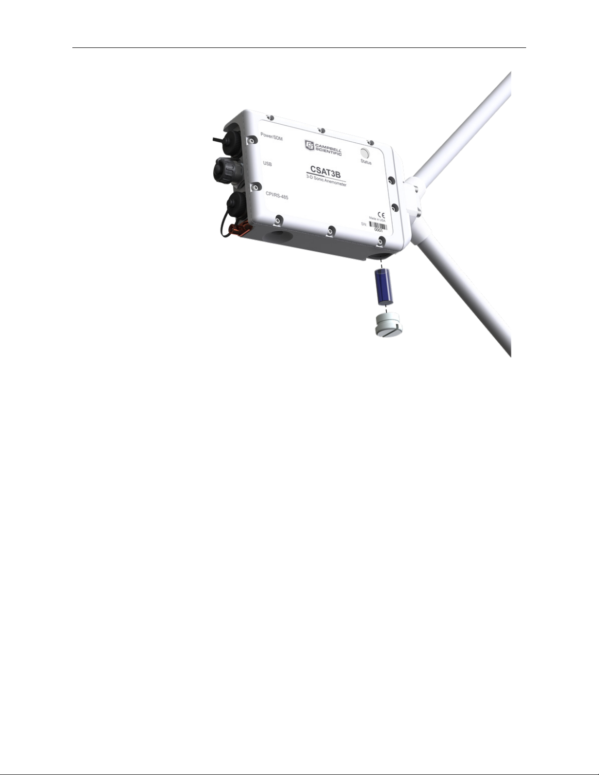
CSAT3B Three-Dimensional Sonic Anemometer
FIGURE 9-2. Exploded view of CSAT3B desiccant canister
9.4 Calibration
The CSAT3B is calibrated at the factory over the temperature range of
−30 to 50 °C, as sonic transducer response is a function of temperature. Any
measurements taken at temperatures outside of this range will be suspect.
The CSAT3B does not require field calibration; however, it may require a
factory recalibration every few years. An indication that the CSAT3B is due to
be returned to the factory for recalibration is when diagnostic flags are
persistent under dry conditions with little to no wind and with no obstruction in
the ultrasonic paths. A wind offset greater than the specifications found in
Section 6, Specifications
To check for wind offset, refer to Section 9.4.1, Test for Wind Offset
9.4.1 Test for Wind Offset
Testing wind offset on a CSAT3B requires creating an environment where
there is no wind. Because it is difficult to do this in the field, wind offset data
from the CSAT3B should be collected in a field office or the lab. A zero-wind
environment can be created with a kitchen waste bin liner. The following steps
should be taken to test the CSAT3B for wind offset.
(p. 18), is another indication that a recalibration is due.
(p. 64).
1. Mount the head using the horizontal mount boom (as described in
Section 4.1, Hardware Connections
(p. 2)), or hang the head from the
block that supports the CSAT3B upper and lower arms. Do not lay the
CAST3B head on its side or balance it on the transducers, as this will
affect its measurements.
64
Page 70
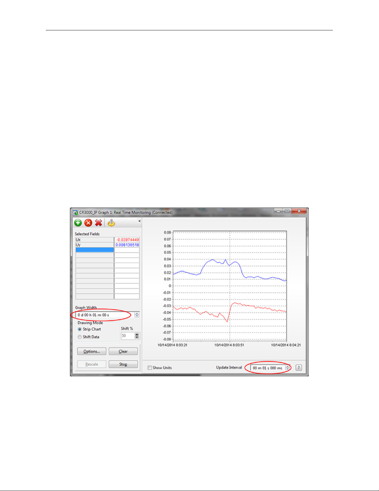
CSAT3B Three-Dimensional Sonic Anemometer
2. Cover the CSAT3B head with a medium (13-gallon) kitchen waste bin
liner. Close the opening of the liner by folding, taping, or tying, to
prevent air from moving in and out of the liner. Temporarily disable
the HVAC system in the room, or cover air vents that may cause air
drafts to pass by the CSAT3B. Ensure that the liner does not obstruct
any of the three CSAT3B sonic paths.
3. Connect the CSAT3B power and communications cable to the data
logger referring to Section 4.2, Communications Connections
(p. 4).
Connect to the data logger with LoggerNet, PC400, or PC200W.
4. Use the real time monitoring graph display to create two graphs.
a. On the first graph add the u
and uy wind components and set
x
the y limits from −0.08 to 0.08 as shown in FIGURE 9-3.
b. On the second graph add the u
wind component and set the y
z
limits from −0.04 to 0.04 as shown in FIGURE 9-4.
c. For both graphs, set Graph Width to 1 minute and Update
Interval to 1 second.
FIGURE 9-3. CSAT3B real-time data with 1 sec update and u
wind component graphed
and uy
x
65
Page 71
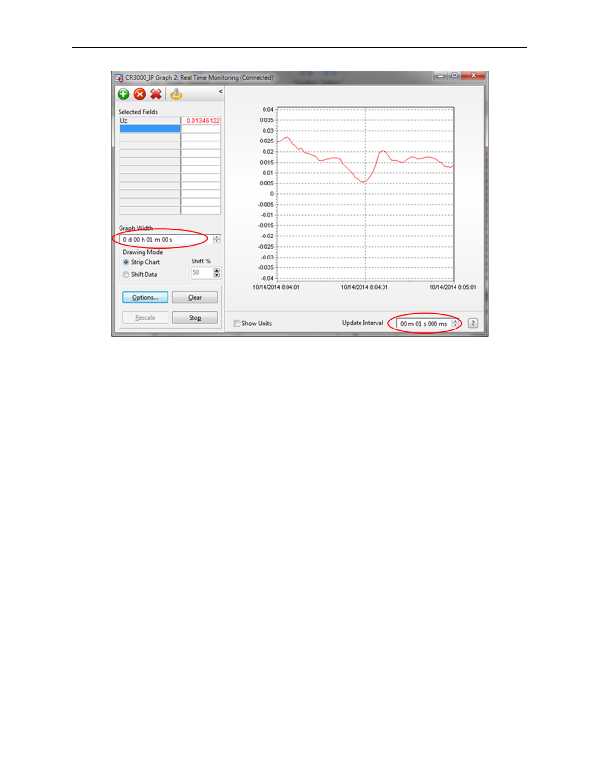
CSAT3B Three-Dimensional Sonic Anemometer
NOTE
FIGURE 9-4. CSAT3B real-time data with 1 sec update and u
component graphed
Graph 1 minute of wind data from the CSAT3B while it is in the zero wind
environment. The wind offset should be less than ± 8 cm·s
, and less than ± 4 cm·s–1 (0.04 m·s–1) for uz. If the CSAT3B wind offset
and u
y
is greater than these specifications, contact Campbell Scientific for an RMA
number to recalibrate the CSAT3B.
When returning a CSAT3B for factory recalibration or repair, it is
important to ship the unit with the foam inserts (see Section
5.2.2.2, Sonic Carrying Case (p. 10)) provided from the factory.
9.5 Troubleshooting
Most problems that occur with the CSAT3B will generate a flag in the
Diagnostic Word that are set high (see Section 8.4.2, Diagnostic Word
and TABLE 8-6). It is normal to see occasional sonic flags being set due to
precipitation, insects, spider webs, birds, etc. that pass through one or more of
the sonic paths and obstruct the signal. If diagnostic flags are persistently high,
however, this could indicate a more serious problem. In the case that diagnostic
flags are persistent, troubleshoot with the following steps:
wind
z
–1
(0.08 m·s–1) for ux
(p. 59),
1. Perform a visual inspection of the CSAT3B. Make sure it is clear
from anything that might obstruct the sonic signal. Check for signs
that the geometry of the arms has changed in any way, possibly from
an impact from another object.
2. Check all wiring connections between the CSAT3B and data logger.
66
Page 72

3. Check to see if the diagnostic flags are still high.
4. If diagnostic flags persist, remove the CSAT3B from the site and
perform a zero-wind offset as described in Section 9.4.1, Test for
Wind Offset
(p. 64). Check to see if the diagnostic flags are any different
once inside the laboratory.
5. In case the diagnostic flags are related to a bug or corruption of the
OS, send a new OS following the instructions in Section 9.5.1,
Sending an OS to the CSAT3B
6. If the problems are still unresolved, contact Campbell Scientific. If
possible, be prepared to send a file of CSAT3B output data, including
the diagnostic word, to Campbell Scientific. If it is determined that the
unit must be returned to the factory for recalibration and/or repair an
RMA will be required (see Section 9.6, Returning the CSAT3B
9.5.1 Sending an OS to the CSAT3B
To send an operating system (OS) to the CSAT3B, follow these steps:
1. Go to www.campbellsci.com/downloads to download the latest version
of the CSAT3B OS to your computer.
CSAT3B Three-Dimensional Sonic Anemometer
(p. 67).
(p. 68)).
2. Connect to the CSAT3B and launch the Device Configuration Utility
as described in Section 7.1, Settings
(p. 23).
3. After connecting to the CSAT3B, click on the Send OS tab at the top
of the Device Configuration Utility main screen. Click on the Start
button at the bottom of the page, select the .obj file that you
downloaded from the Campbell website, and click Open. The OS will
then be sent, followed by a confirmation message that it was loaded
properly.
67
Page 73

CSAT3B Three-Dimensional Sonic Anemometer
FIGURE 9-5. The Send OS screen in the Device Configuration Utility
9.6 Returning the CSAT3B
If there is need to return the CSAT3B either for calibration or repair, please
follow the detailed instructions provided in the Assistance section at the back
of this manual which gives instructions for generating an RMA number. If
additional help is needed, please contact Campbell Scientific. When preparing
the CSAT3B for shipment, be sure to package it in the same foam that it was
sent in. If the foam cannot be found, new foam should be ordered from
Campbell Scientific before returning the unit.
10. Reference and Attributions
10.1 References
Liu, H., Peters, G. and Foken, T.: 2001, “New Equations for Sonic
Temperature Variance and Buoyancy Heat Flux with an Omnidirectional
Sonic Anemometer”, Boundary-Layer Meteorol., 100, 459 – 468.
Kaimal, J.C.: 1979, “Sonic anemometer measurement of atmospheric
turbulence”, Proceeding of the Dynamic Flow Conference, Skovlunde.
DISA Electronic A/S, 551 – 565.
Horst, T.W., Semmer, S.R., and Maclean, G.: 2015, “Correction of a Non-
orthogonal, Three-Component Sonic Anemometer for Flow Distortion by
Transducer Shadowing”, Boundary-Layer Meteorol, 155, 371 – 395. DOI
10.1007/s10546-015-0010-3.
68
Page 74

CSAT3B Three-Dimensional Sonic Anemometer
Schotanus, P., Nieuwstadt, F. T. M. and de Bruin, H. A. R.: 1983,
“Temperature Measurement with a Sonic Anemometer and its Application
to Heat and Moisture Fluxes”, Boundary-Layer Meteorol., 26, 81 – 93.
Burns, S. P., Horst, T. W., Jacobsen, L., Blanken P. D. and Monson, R. K.:
2012, “Using sonic anemometer temperature to measure sensible heat flux
in strong winds”, Atmos. Meas. Tech., 5, 2095 – 2111.
Kaimal, J. C. and Finnigan J. J.: 1994, “Atmospheric Boundary Layer Flows”,
Oxford University Press.
69
Page 75
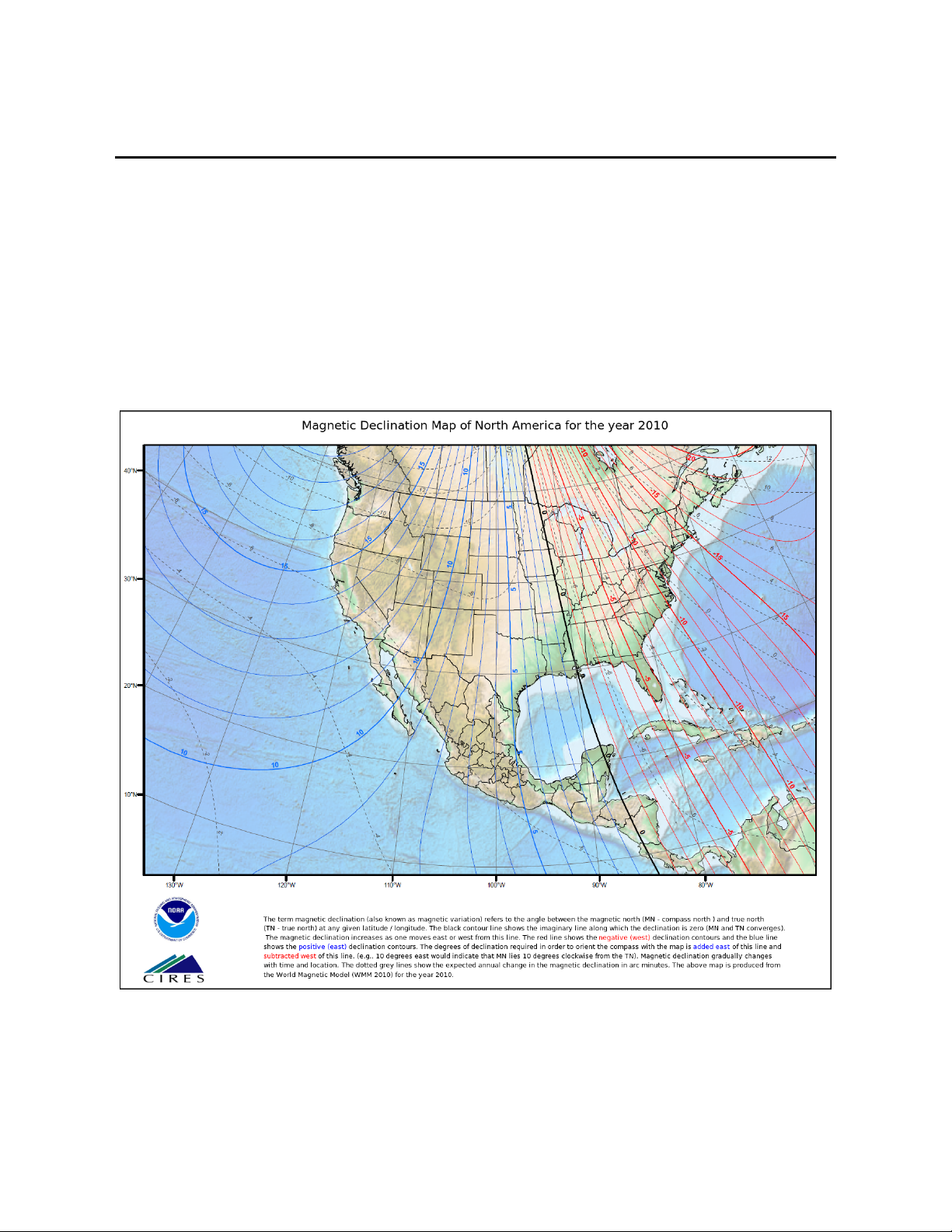
Appendix A. CSAT3B Orientation
A.1 Determining True North and Sensor Orientation
The orientation of the CSAT3B negative x-axis is found by reading a magnetic
compass and applying the site-specific correction for magnetic declination;
where the magnetic declination is the number of degrees between True North
and Magnetic North. Magnetic declination for a specific site can be obtained
from a USGS map, local airport, or through a NOAA web calculator
(Appendix A.2, Online Magnetic Declination Calculator
map in FIGURE A-1 taken from
www.ngdc.noaa.gov/geomag/img/DeclinationMap_US.png shows magnetic
declination for the conterminous United States in 2010.
(p. A-3)). A general
FIGURE A-1. Magnetic declination for the conterminous United States
(2010)
A-1
Page 76

Appendix A. CSAT3B Orientation
Declination angles are always subtracted from the compass reading to find
True North. A declination angle East of True North is reported as positive a
value and is subtracted from 360 (0) degrees to find True North as shown
FIGURE A-2. A declination angle West of True North is reported as a negative
value and is also subtracted from 0 (360) degrees to find True North as shown
in FIGURE A-3. Note that when a negative number is subtracted from a
positive number, the resulting arithmetic operation is addition.
For example, the declination for Longmont, CO (10 June 2006) is 9.67 degrees
(the angle is East of True North, so it is reported as positive), thus True North
is 360 degrees ˗ 9.67 degrees, or 350.33 degrees as read on a compass.
Likewise, the declination for Mc Henry, IL (10 June 2006) is ˗ 2.68 degrees,
and True North is 0 degrees ˗ (˗ 2.68 degrees), or 2.68 degrees as read on a
compass.
FIGURE A-2. A declination angle east of true north (positive) is
subtracted from 360 (0) degrees to find true north
FIGURE A-3. A declination angle west of true north (negative) is
subtracted from 0 (360) degrees to find true north
A-2
Page 77

Appendix A. CSAT3B Orientation
A.2 Online Magnetic Declination Calculator
The magnetic declination calculator web calculator published by NOAA’s
Geophysical Data Center is available at the following URL:
www.ngdc.noaa.gov/geomag-web/#declination. After the web page loads, enter
the zip code, country and city, or latitude and longitude of the site, then click
on Calculate to get the declination for that site (FIGURE A-4).
FIGURE A-4. NOAA magnetic declination calculator
A-3
Page 78

Appendix A. CSAT3B Orientation
FIGURE A-5. NOAA magnetic calculator results
The declination for Salt Lake City, UT is 11.7 degrees (4 November, 2014). As
shown in FIGURE A-5, the declination for Utah is positive (east of north), so
true north for this site is 360 – 11.7, or 348.3 degrees. The annual change is
–7.8 minutes/year or 7.8 minutes west per year.
A-4
Page 79

t
d
c u
o
a
=
+
t
d
c u
b
=
-
a
u
d
t t
a
o b
= −
2
1 1
u
uuAuu
u
x
y
z
a
b
c
=
Appendix B. CSAT3B Measurement Theory
B.1 Theory of Operation
B.1.1 Wind Speed
Each axis of the CSAT3B pulses two ultrasonic signals in opposite directions.
The time of flight of the first signal (out) is given by:
and the time of flight of the second signal (back) is given by:
where: t
t
u
d = distance between the transducers
c = speed of sound
The wind speed, u
relationships, then subtracting Eq. (B-2) from (B-1) and solving for u
= time of flight out along the transducer axis
o
= time of flight back, in the opposite direction
b
= wind speed along the transducer axis
a
, along any axis can be found by inverting the above
a
(B-1)
(B-2)
(B-3)
.
a
The wind speed is measured on all three non-orthogonal axis to give u
, where the subscripts a, b, and c refer to the non-orthogonal sonic axis.
u
c
The non-orthogonal wind speed components are then transformed into
orthogonal wind speed components, u
where: A = a 3 x 3 coordinate transformation matrix, that is unique
for each CSAT3B and is stored in ROM memory
, uy, and uz, with the following:
x
(B-4)
, ub, and
a
B-1
Page 80

B.1.2 Temperature
c
d
t t
o b
= +
2
1
1
( )
qTRTRPc
dvd
61.01
2
+===
γγργ
C
p
= + −qC q C
pw pd
( )1
= +C
q
pd
( . )1 0 84
C
v
= + −qC q C
vw vd
( )1
= +C
q
vd
( . )
1 0 93
The sonically determined speed of sound is given in Eq. (B-5) and was found
from the sum of the inverses of Eq. (B-1) and (B-2). The CSAT3B corrects
online for the effect of wind blowing perpendicular to the sonic path. No
additional off-line corrections are required as suggested by Liu et al., 2001.
Appendix B. CSAT3B Measurement Theory
The speed of sound in moist air is a function of temperature and humidity and
is given by:
where: γ = ratio of specific heat of moist air at constant pressure to
that at constant volume
P = pressure
ρ = air density
R
T
T = air temperature
q = specific humidity defined as the ratio of the mass of
= gas constant for dry air
d
= virtual temperature
v
water vapor to the total mass of air (as in Kaimal and
Gaynor, 1991; and Wallace and Hobbs, 1977)
(B-5)
(B-6)
Note that γ is a function of specific humidity. It would be convenient if the
effects of humidity could be consolidated into one term.
The specific heats for moist air at constant pressure and volume are given by:
where: C
and pressure
C
and Cv = specific heats of moist air at constant volume
p
and Cvw = specific heat of water vapor
pw
(B-7a)
(B-7b)
B-2
Page 81

Appendix B. CSAT3B Measurement Theory
c R T R T q
d
d
s d d
2
1 0 51= = +γ γ ( . )
T
c
R
s
d d
= −2273 15γ.
C
and Cvd = specific heat of dry air, respectively (Fleagle
pd
and Businger, 1980)
Substitute Eq. (B-7a) and (B-7b) into (B-6) and ignore the higher order terms.
This yields
where: T
γ
= sonic virtual temperature
s
= ratio of specific heat of dry air at constant pressure to
d
(B-8)
that at constant volume (Fleagle and Businger, 1980; Kaimal
and Gaynor, 1991; Kaimal and Businger, 1963; Schotanus et
al., 1983)
With Eq. (B-8), the effect of humidity, on the speed of sound, is included in the
sonic virtual temperature.
The sonic virtual temperature, in degrees Celsius, is given by Eq. (B-9), where
= 1.4 and Rd = 287.04 JK-1 kg-1.
γ
d
(B-9)
B.2 References
Kaimal, J. C. and Businger, J. A.: 1963, “A Continuous Wave Sonic
Anemometer-Thermometer”, J. Applied Meteorol., 2, 156-164.
Kaimal, J. C. and Gaynor, J. E.: 1991, “Another Look at Sonic Thermometry”,
Boundary-Layer Meteorol., 56, 401-410.
Fleagle, R. G. and Businger, J. A.: 1980, An Introduction to Atmospheric
Physics, Academic Press, Inc., New York.
Liu, H., Peters, G. and Foken, T.: 2001, “New Equations for Sonic
Temperature Variance and Buoyancy Heat Flux with an Omnidirectional Sonic
Anemometer”, Boundary-Layer Meteorol., 100, 459-468.
Schotanus, P., Nieuwstadt, F. T. M. and de Bruin, H. A. R.: 1983,
“Temperature Measurement with a Sonic Anemometer and its Application to
Heat and Moisture Fluxes”, Boundary-Layer Meteorol., 26, 81-93.
Wallace, J. M. and Hobbs, P. V.: 1977, Atmospheric Science an Introductory
Survey, Academic Press, Inc., New York.
B-3
Page 82

Limited Warranty
Products manufactured by Campbell Scientific are warranted by Campbell
Scientific to be free from defects in materials and workmanship under normal
use and service for twelve months from the date of shipment unless otherwise
specified on the corresponding product webpage. See Product Details on the
Ordering Information pages at www.campbellsci.com. Other manufacturer's
products, that are resold by Campbell Scientific, are warranted only to the
limits extended by the original manufacturer.
Refer to www.campbellsci.com/terms#warranty for more information.
CAMPBELL SCIENTIFIC EXPRESSLY DISCLAIMS AND
EXCLUDES ANY IMPLIED WARRANTIES OF MERCHANTABILITY
OR FITNESS FOR A PARTICULAR PURPOSE. Campbell Scientific
hereby disclaims, to the fullest extent allowed by applicable law, any and
all warranties and conditions with respect to the Products, whether
express, implied or statutory, other than those expressly provided herein.
Page 83

Assistance
Products may not be returned without prior authorization.
Products shipped to Campbell Scientific require a Returned Materials
Authorization (RMA) or Repair Reference number and must be clean and
uncontaminated by harmful substances, such as hazardous materials,
chemicals, insects, and pests. Please complete the required forms prior to
shipping equipment.
Campbell Scientific regional offices handle repairs for customers within their
territories. Please see the back page for the Global Sales and Support Network
or visit www.campbellsci.com/contact to determine which Campbell Scientific
office serves your country.
To obtain a Returned Materials Authorization or Repair Reference number,
contact your CAMPBELL SCIENTIFIC regional office. Please write the
issued number clearly on the outside of the shipping container and ship as
directed.
For all returns, the customer must provide a “Statement of Product Cleanliness
and Decontamination” or “Declaration of Hazardous Material and
Decontamination” form and comply with the requirements specified in it. The
form is available from your CAMPBELL SCIENTIFIC regional office.
Campbell Scientific is unable to process any returns until we receive this
statement. If the statement is not received within three days of product receipt
or is incomplete, the product will be returned to the customer at the customer’s
expense. Campbell Scientific reserves the right to refuse service on products
that were exposed to contaminants that may cause health or safety concerns for
our employees.
Page 84

Safety
DANGER — MANY HAZARDS ARE ASSOCIATED WITH INSTALLING, USING, MAINTAINING, AND WORKING ON OR AROUND
TRIPODS, TOWERS, AND ANY ATTACHMENTS TO TRIPODS AND TOWERS SUCH AS SENSORS, CROSSARMS, ENCLOSURES,
ANTENNAS, ETC. FAILURE TO PROPERLY AND COMPLETELY ASSEMBLE, INSTALL, OPERATE, USE, AND MAINTAIN TRIPODS,
TOWERS, AND ATTACHMENTS, AND FAILURE TO HEED WARNINGS, INCREASES THE RISK OF DEATH, ACCIDENT, SERIOUS
INJURY, PROPERTY DAMAGE, AND PRODUCT FAILURE. TAKE ALL REASONABLE PRECAUTIONS TO AVOID THESE HAZARDS.
CHECK WITH YOUR ORGANIZATION'S SAFETY COORDINATOR (OR POLICY) FOR PROCEDURES AND REQUIRED PROTECTIVE
EQUIPMENT PRIOR TO PERFORMING ANY WORK.
Use tripods, towers, and attachments to tripods and towers only for purposes for which they are designed. Do not exceed design limits. Be familiar and
comply with all instructions provided in product manuals. Manuals are available at www.campbellsci.com. You are responsible for conformance with
governing codes and regulations, including safety regulations, and the integrity and location of structures or land to which towers, tripods, and any
attachments are attached. Installation sites should be evaluated and approved by a qualified engineer. If questions or concerns arise regarding installation,
use, or maintenance of tripods, towers, attachments, or electrical connections, consult with a licensed and qualified engineer or electrician.
General
• Protect from over-voltage.
• Protect electrical equipment from water.
• Protect from electrostatic discharge (ESD).
• Protect from lightning.
• Prior to performing site or installation work, obtain required approvals and permits. Comply with all
governing structure-height regulations.
• Use only qualified personnel for installation, use, and maintenance of tripods and towers, and any
attachments to tripods and towers. The use of licensed and qualified contractors is highly recommended.
• Read all applicable instructions carefully and understand procedures thoroughly before beginning work.
• Wear a hardhat and eye protection, and take other appropriate safety precautions while working on or
around tripods and towers.
• Do not climb tripods or towers at any time, and prohibit climbing by other persons. Take reasonable
precautions to secure tripod and tower sites from trespassers.
• Use only manufacturer recommended parts, materials, and tools.
Utility and Electrical
• You can be killed or sustain serious bodily injury if the tripod, tower, or attachments you are installing,
constructing, using, or maintaining, or a tool, stake, or anchor, come in contact with overhead or
underground utility lines.
• Maintain a distance of at least one-and-one-half times structure height, 6 meters (20 feet), or the distance
required by applicable law, whichever is greater, between overhead utility lines and the structure (tripod,
tower, attachments, or tools).
• Prior to performing site or installation work, inform all utility companies and have all underground utilities
marked.
• Comply with all electrical codes. Electrical equipment and related grounding devices should be installed by a
licensed and qualified electrician.
• Only use power sources approved for use in the country of installation to power Campbell Scientific devices.
Elevated Work and Weather
• Exercise extreme caution when performing elevated work.
• Use appropriate equipment and safety practices.
• During installation and maintenance, keep tower and tripod sites clear of un-trained or non-essential
personnel. Take precautions to prevent elevated tools and objects from dropping.
• Do not perform any work in inclement weather, including wind, rain, snow, lightning, etc.
Maintenance
• Periodically (at least yearly) check for wear and damage, including corrosion, stress cracks, frayed cables,
loose cable clamps, cable tightness, etc. and take necessary corrective actions.
• Periodically (at least yearly) check electrical ground connections.
Internal Battery
• Be aware of fire, explosion, and severe-burn hazards.
• Misuse or improper installation of the internal lithium battery can cause severe injury.
• Do not recharge, disassemble, heat above 100 °C (212 °F), solder directly to the cell, incinerate, or expose
contents to water. Dispose of spent batteries properly.
WHILE EVERY ATTEMPT IS MADE TO EMBODY THE HIGHEST DEGREE OF SAFETY IN ALL CAMPBELL SCIENTIFIC PRODUCTS, THE
CUSTOMER ASSUMES ALL RISK FROM ANY INJURY RESULTING FROM IMPROPER INSTALLATION, USE, OR MAINTENANCE OF
TRIPODS, TOWERS, OR ATTACHMENTS TO TRIPODS AND TOWERS SUCH AS SENSORS, CROSSARMS, ENCLOSURES, ANTENNAS,
ETC.
Page 85

Campbell Scientific regional offices
Australia
Location:
Phone:
Email:
Website:
Brazil
Location:
Phone:
Email:
Website:
Canada
Location:
Phone:
Email:
Website:
China
Location:
Phone:
Email:
Website:
Garbutt, QLD Australia
61.7.4401.7700
info@campbellsci.com.au
www.campbellsci.com.au
São Paulo, SP Brazil
11.3732.3399
vendas@campbellsci.com.br
www.campbellsci.com.br
Edmonton, AB Canada
780.454.2505
dataloggers@campbellsci.ca
www.campbellsci.ca
Beijing, P. R. China
86.10.6561.0080
info@campbellsci.com.cn
www.campbellsci.com.cn
France
Location:
Phone:
Email:
Website:
Vincennes, France
0033.0.1.56.45.15.20
info@campbellsci.fr
www.campbellsci.fr
Germany
Location:
Phone:
Email:
Website:
Bremen, Germany
49.0.421.460974.0
info@campbellsci.de
www.campbellsci.de
India
Location:
Phone:
Email:
Website:
New Delhi, DL India
91.11.46500481.482
info@campbellsci.in
www.campbellsci.in
South Africa
Location:
Phone:
Email:
Website:
Stellenbosch, South Africa
27.21.8809960
sales@campbellsci.co.za
www.campbellsci.co.za
Thailand
Location:
Phone:
Email:
Website:
UK
Location:
Phone:
Email:
Website:
USA
Location:
Phone:
Email:
Website:
Bangkok, Thailand
66.2.719.3399
info@campbellsci.asia
www.campbellsci.asia
Shepshed, Loughborough, UK
44.0.1509.601141
sales@campbellsci.co.uk
www.campbellsci.co.uk
Logan, UT USA
435.227.9120
info@campbellsci.com
www.campbellsci.com
Costa Rica
Location:
Phone:
Email:
Website:
San Pedro, Costa Rica
506.2280.1564
info@campbellsci.cc
www.campbellsci.cc
Spain
Location:
Phone:
Email:
Website:
Barcelona, Spain
34.93.2323938
info@campbellsci.es
www.campbellsci.es
 Loading...