Campbell Scientific 253-L User Manual

253-L and 257-L

Soil Matric Potential Sensors

Revision: 9/13

Copyright © 1993-2013

Campbell Scientific, Inc.

Warranty

“PRODUCTS MANUFACTURED BY CAMPBELL SCIENTIFIC, INC. are
warranted by Campbell Scientific, Inc. (“Campbell”) to be free from defects in
materials and workmanship under normal use and service for twelve (12)
months from date of shipment unless otherwise specified in the corresponding
Campbell pricelist or product manual. Products not manufactured, but that are
re-sold by Campbell, are warranted only to the limits extended by the original
manufacturer. Batteries, fine-wire thermocouples, desiccant, and other
consumables have no warranty. Campbell’s obligation under this warranty is
limited to repairing or replacing (at Campbell’s option) defective products,
which shall be the sole and exclusive remedy under this warranty. The
customer shall assume all costs of removing, reinstalling, and shipping
defective products to Campbell. Campbell will return such products by surface
carrier prepaid within the continental United States of America. To all other
locations, Campbell will return such products best way CIP (Port of Entry)
INCOTERM® 2010, prepaid. This warranty shall not apply to any products
which have been subjected to modification, misuse, neglect, improper service,
accidents of nature, or shipping damage. This warranty is in lieu of all other
warranties, expressed or implied. The warranty for installation services
performed by Campbell such as programming to customer specifications,
electrical connections to products manufactured by Campbell, and product
specific training, is part of Campbell’s product warranty. CAMPBELL
EXPRESSLY DISCLAIMS AND EXCLUDES ANY IMPLIED
WARRANTIES OF MERCHANTABILITY OR FITNESS FOR A
PARTICULAR PURPOSE. Campbell is not liable for any special, indirect,
incidental, and/or consequential damages.”

Assistance

Products may not be returned without prior authorization. The following
contact information is for US and international customers residing in countries
served by Campbell Scientific, Inc. directly. Affiliate companies handle
repairs for customers within their territories. Please visit

www.campbellsci.com to determine which Campbell Scientific company serves

your country.

To obtain a Returned Materials Authorization (RMA), contact CAMPBELL
SCIENTIFIC, INC., phone [phone]. After an applications engineer
determines the nature of the problem, an RMA number will be issued. Please
write this number clearly on the outside of the shipping container. Campbell
Scientific’s shipping address is:

CAMPBELL SCIENTIFIC, INC.
RMA#_____
815 West 1800 North
Logan, Utah 84321-1784

For all returns, the customer must fill out a “Statement of Product Cleanliness
and Decontamination” form and comply with the requirements specified in it.
The form is available from our web site at www.campbellsci.com/repair. A
completed form must be either emailed to [e-mail] or faxed to
[phone]. Campbell Scientific is unable to process any returns until we
receive this form. If the form is not received within three days of product
receipt or is incomplete, the product will be returned to the customer at the
customer’s expense. Campbell Scientific reserves the right to refuse service on
products that were exposed to contaminants that may cause health or safety
concerns for our employees.

Table of Contents

PDF viewers: These page numbers refer to the printed version of this document. Use the
PDF reader bookmarks tab for links to specific sections.

1. Introduction.................................................................1

2. Cautionary Statements...............................................1

3. Initial Inspection .........................................................1

4. Quickstart .................................................................... 2

4.1 Installation/Removal ............................................................................2

4.2 Use SCWin to Program Datalogger and Generate Wiring Diagram....3

4.2.1 257 SCWin Programming.............................................................3

4.2.2 253 SCWin Programming.............................................................7

5. Overview....................................................................12

6. Specifications ...........................................................13

7. Operation...................................................................14

7.1 Wiring ................................................................................................14

7.1.1 257 Wiring ..................................................................................14

7.1.2 253 Wiring ..................................................................................14

7.2 Programming......................................................................................15

7.2.1 CRBasic Dataloggers ..................................................................15

7.2.1.1 BRHalf Instruction ...........................................................15

7.2.1.2 Resistance Calculation .....................................................16

7.2.2 Edlog Dataloggers.......................................................................16

7.2.2.1 Program Instruction 5.......................................................16

7.2.2.2 Program Instruction 59.....................................................16

7.2.3 Calculate Soil Water Potential ....................................................17

7.2.3.1 Linear Relationship ..........................................................17

7.2.3.2 Non-Linear Relationship ..................................................18

7.2.3.3 Soil Water Matric Potential in Other Units ......................19

7.3 Example Programs .............................................................................19

7.3.1 257 Program Examples ...............................................................19

7.3.1.1 Program Example #1 — CR1000 with One 107 and

One 257.........................................................................19

7.3.1.2 Program Example #2 — CR10X with One 107 and

One 257.........................................................................20

7.3.2 253 Program Examples ...............................................................22

7.3.2.1 Program Example #3 — Five 107 Temperature Probes

and Five 253’s on AM16/32 and CR1000 ....................22

i

Table of Contents

7.3.2.2

Program Example #4 — Five 107 Temperature Probes

and Five 253’s on AM16/32 and CR10X Using Non-

Linear Equation............................................................ 24

7.4 Interpreting Results ........................................................................... 27

8. Troubleshooting........................................................27

9. Reference...................................................................28

Figures

5-1. 257 Soil Matric Potential Sensor with capacitor circuit and

completion resistor installed in cable. Model 253 is the same,

except that it does not have completion circuitry in the cable. ...... 13

7-1. 257 schematic.................................................................................... 14

7-2. 253 wiring example ........................................................................... 15

Tables

7-1. Excitation and Voltage Ranges for CRBasic Dataloggers................. 16

7-2. Excitation and Voltage Ranges for Edlog Dataloggers ..................... 16

7-3. Comparison of Estimated Soil Water Potential and Rs at 21°C......... 18

7-4. Conversion of Matric Potential to Other Units.................................. 19

7-5. Wiring for Programming Example #1............................................... 19

7-6. Wiring for Programming Example #2............................................... 20

7-7. Wiring for Programming Example #3............................................... 23

7-8. Wiring for Programming Example #4............................................... 24

ii

253-L and 257-L Soil Matric Potential
Sensors

1. Introduction

The 253 and 257 soil matric potential sensors are solid-state, electrical­resistance sensing devices with a granular matrix that estimate soil water
potential between 0 and –2 bars (typically wetter or irrigated soils).

The 253 needs to be connected to an AM16/32-series multiplexer, and is
intended for applications where a larger number of sensors will be monitored.
The 257 connects directly to our dataloggers.

Before using a 253 or 257, please study:

• Section 2, Cautionary Statements

• Section 3, Initial Inspection

• Section 4, Quickstart

2. Cautionary Statements

• The black outer jacket of the cable is Santoprene® rubber. This jacket will

support combustion in air. It is rated as slow burning when tested
according to U.L. 94 H.B. and will pass FMVSS302. Local fire codes
may preclude its use inside buildings.

• Avoid installing in depressions where water will puddle after a rain storm.

• Don’t place the 253 or 257 in high spots or near changes in slope unless

wanting to measure the variability created by such differences.

• When removing the sensor prior to harvest of annual crops, do so just after

the last irrigation when the soil is moist.

• When removing a sensor, do not pull the sensor out by its wires.

• Careful removal prevents sensor and membrane damage.

3. Initial Inspection

• Upon receipt of a 253 or 257, inspect the packaging and contents for

damage. File damage claims with the shipping company.

• The model number and cable length are printed on a label at the

connection end of the cable. Check this information against the shipping
documents to ensure the correct product and cable length are received.

1

253-L and 257-L Soil Matric Potential Sensors

4. Quickstart

Please review Section 7, Operation, for wiring, CRBasic programming, Edlog
programming, and interpretation of results.

4.1 Installation/Removal

NOTE

Placement of the sensor is important. To acquire representative
measurements, avoid high spots, slope changes, or depressions
where water puddles. Typically, the sensor should be located in
the root system of the crop.

1. Soak sensors in water for one hour then allow them to dry, ideally for 1 to

2 days.

2. Repeat Step 1 twice if time permits.

3. Make the sensor access holes to the required depth. Often, a 22 mm (7/8

in) diameter rod can be used to make the hole. However, if the soil is very
coarse or gravelly, an oversized hole (25 to 32 mm) may be required to
prevent abrasion damage to the sensor membrane. The ideal method of
making an oversized access hole is to have a stepped tool that makes an
oversized hole for the upper portion and an exact size hole for the lower
portion.

4. If the hole is oversized (25 to 32 mm), mix a slurry of soil and water to a

creamy consistency and place it into the sensor access hole.

5. Insert the sensors in the sensor access hole. A length of 1/2 inch class 315

PVC pipe fits snugly over the sensor collar and can be used to push in the
sensor. The PVC can be left in place with the wires threaded through the
pipe and the open end taped shut (duct tape is adequate). This practice
also simplifies the removal of the sensors. When using PVC piping,
solvent weld the PVC pipe to the sensor collar. Use PVC/ABS cement on
the stainless steel sensors with the green top. Use clear PVC cement only
on the PVC sensors with the gray top.

2

NOTE

CAUTION

6. Force the soil or slurry to envelope the sensors. This will ensure uniform

soil contact.

Snug fit in the soil is extremely important. Lack of a snug fit is
the premier problem with sensor effectiveness.

7. Carefully, back fill the hole, and tamp down to prevent air pockets which

could allow water to channel down to the sensor.

8. When removing sensors prior to harvest in annual crops, do so just after

the last irrigation when the soil is moist.

Do not pull the sensor out by the wires. Careful removal
prevents sensor and membrane damage.

253-L and 257-L Soil Matric Potential Sensors

9. When sensors are removed for winter storage, clean, dry, and place them

in a plastic bag.

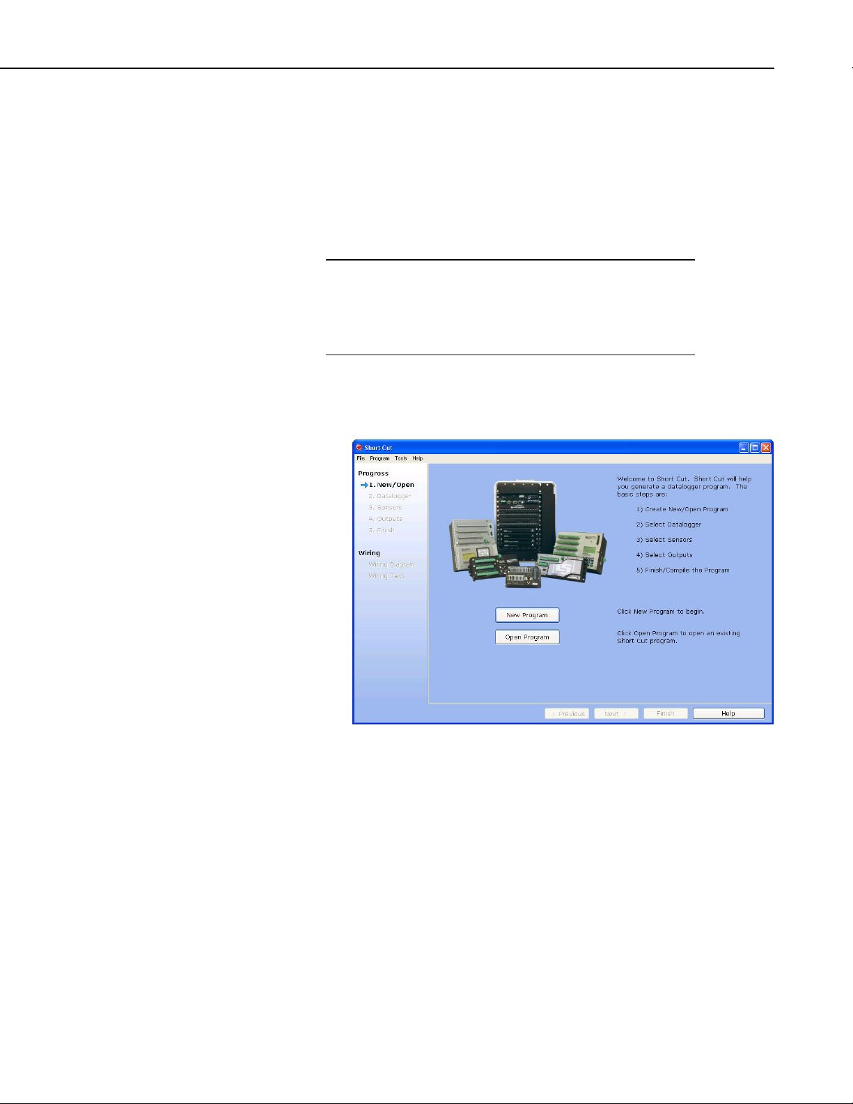
4.2 Use SCWin to Program Datalogger and Generate Wiring Diagram

The simplest method for programming the datalogger to measure the sensor is
to use Campbell Scientific’s SCWin Program Generator (Short Cut).

NOTE

Short Cut requires the use of a soil temperature sensor before the
253 or 257 sensor is added. This is needed because there is a
temperature correction factor in the equations that convert sensor
resistance. In these Quickstart examples, a 107-L temperature
probe is used to measure soil temperature.

4.2.1 257 SCWin Programming

1. Open Short Cut and click on New Program.

3

253-L and 257-L Soil Matric Potential Sensors

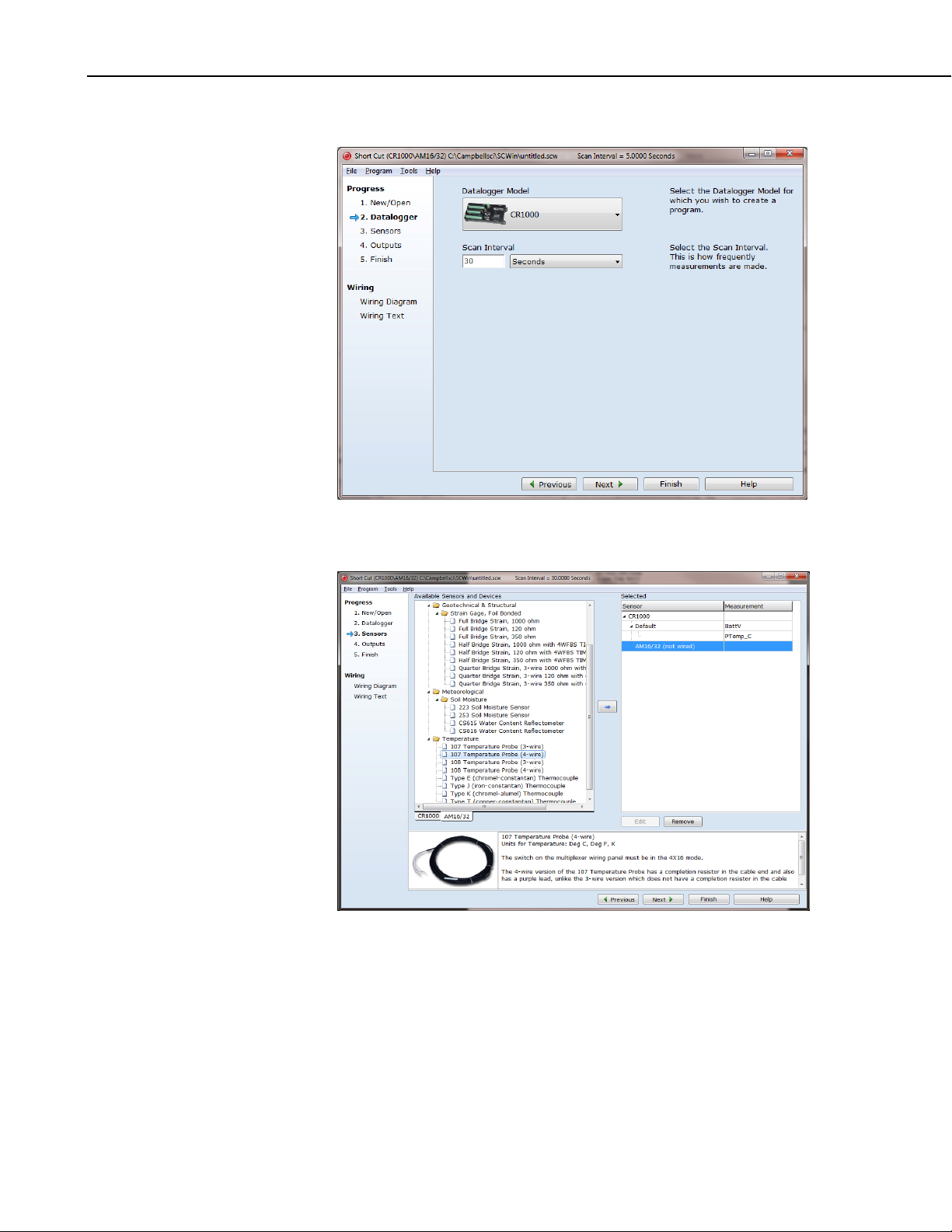
2. Select the datalogger and enter the scan interval, and then select Next.

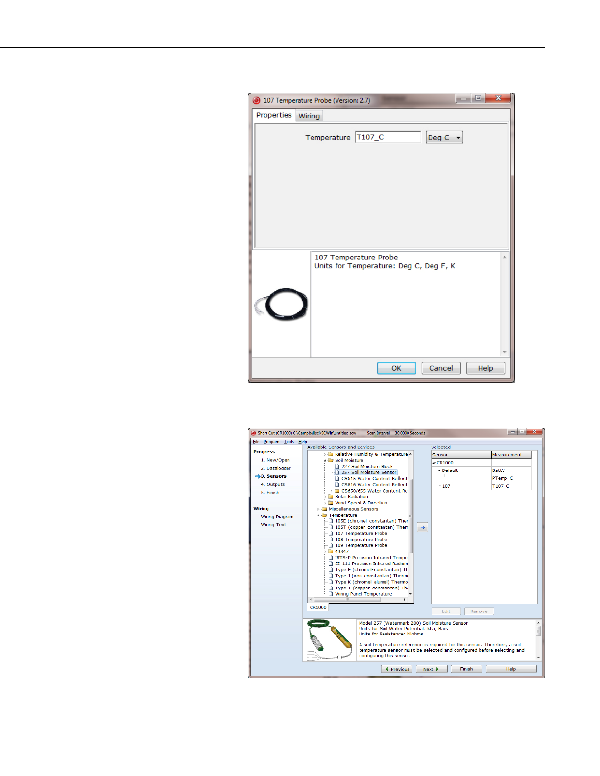
3. Select 107 Temperature Probe and select the right arrow (in center of
screen) to add it to the list of sensors to be measured.

4

253-L and 257-L Soil Matric Potential Sensors

4. Select the 107’s units and click on OK.

5. Select 257 Soil Moisture Sensor, and select the right arrow (in center of
screen) to add it to the list of sensors to be measured.

5

253-L and 257-L Soil Matric Potential Sensors

6. Select the resistance units, soil water units, soil water potential range, and
soil reference temperature. After entering the information, click OK, and
select Next.

7. Choose the outputs and select Finish.

8. In the Save As window, enter an appropriate file name and select Save.

6

9. In the Confirm window, click Yes to download the program to the
datalogger.

253-L and 257-L Soil Matric Potential Sensors

10. Click on Wiring Diagram and wire the 257 and 107 to the CR1000
according to the wiring diagram generated by Short Cut.

4.2.2 253 SCWin Programming

1. Open Short Cut and click New Program.

7

253-L and 257-L Soil Matric Potential Sensors

2. Select the datalogger and enter the scan interval, and select Next.

NOTE

A scan rate of 30 seconds or longer is recommended when using
a multiplexer.

3. Select 107 Temperature Probe and select the right arrow (in center of
screen) to add it to the list of sensors to be measured.

8

253-L and 257-L Soil Matric Potential Sensors

4. Select the 107’s units and click OK.

5. Under Devices, select AM16/32, and select the right arrow (in center of
screen) to add it to the list.

9

253-L and 257-L Soil Matric Potential Sensors

6. Select 253, and select the right arrow (in center of screen) to add it to the
list of sensors to be measured.

7. Select the number of sensors, resistance units, soil water potential units,
soil water potential range, and soil reference temperature. After entering
the information, click OK, and select Next.

10

253-L and 257-L Soil Matric Potential Sensors

8. Choose the outputs and select Finish.

9. In the Save As window, enter an appropriate file name and select Save.

10. In the Confirm window, click Yes to download the program to the
datalogger.

11. Click on Wiring Diagram and select the CR1000 tab. Wire the 107 and
the AM16/32 to the CR1000 according to the wiring diagram generated by
Short Cut.

12. Select the AM16/32 tab and wire the 253 sensors to the AM16/32
according to the wiring diagram generated by Short Cut.

11

253-L and 257-L Soil Matric Potential Sensors

5. Overview

The 253 and 257 soil matric potential sensors provide a convenient method of
estimating water potential of wetter soils in the range of 0 to –200 kPa. The
253 is the Watermark 200 Soil Matric Potential Block modified for use with
Campbell Scientific multiplexers and the 257 is the Watermark 200 Soil Matric
Potential Block modified for use with Campbell Scientific dataloggers.

The –L option on the Model 257-L and 253-L indicates that the cable length is
user specified. This manual refers to the sensors as the 257 and 253. The
typical cable length for the 257 is 25 ft. The following two cable termination
options are offered for the 257:

• Pigtails that connect directly to a Campbell Scientific datalogger

(cable termination option –PT).

• Connector that attaches to a prewired enclosure (cable termination

option –PW).

For 253 applications, most of the cable length used is between the datalogger
and the multiplexer, which reduces overall cable costs and allows each cable
attached to the 253 to be shorter. The cable length of each 253 only needs to
cover the distance from the multiplexer to the point of measurement. Typical
cable length for the 253 is 25 to 50 ft.

The difference between the 253 and the 257 is that there is a capacitor circuit
and completion resistor installed in the 257 cable (FIGURE 5-1) to allow for
direct connection to a datalogger, while the 253 does not have any added
circuitry. For applications requiring many sensors on an analog multiplexer,
the 253 is used and one or more completion resistors are connected to the
datalogger wiring panel. A capacitor circuit is not required for the 253 on a
multiplexer because the electrical connection between the sensor and the
datalogger is interrupted when the multiplexer is deactivated. Any potential
difference between the datalogger earth ground and the electrodes in the sensor
is thus eliminated.

The 253 and 257 consist of two concentric electrodes embedded in a reference
granular matrix material. The granular matrix material is surrounded by a
synthetic membrane for protection against deterioration. An internal gypsum
tablet buffers against the salinity levels found in irrigated soils.

If cultivation practices allow, the sensor can be left in the soil all year,
eliminating the need to remove the sensor during the winter months.

12

253-L and 257-L Soil Matric Potential Sensors

FIGURE 5-1. 257 Soil Matric Potential Sensor with capacitor circuit and

completion resistor installed in cable. Model 253 is the same,
except that it does not have completion circuitry in the cable.

6. Specifications

Features:

Compatible Dataloggers: CR800

CR850
CR1000
CR3000
CR5000
CR9000(X)
CR7
CR10(X)
21X
CR23X
CR500 (257 only)
CR510 (257 only)

• Survives freeze-thaw cycles

• Rugged, long-lasting sensor

• Buffers salts in soil

• No maintenance required

• Compatible with most Campbell Scientific dataloggers

• The 257 contains blocking capacitors in its cable that minimizes

galvanic degradation and measurement errors due to ground loops

• For the 253, the multiplexer connection prevents electrolysis from

prematurely destroying the probe

13

253-L and 257-L Soil Matric Potential Sensors

R

Ω

Range: 0 to –200 kPa

Dimensions: 8.26 cm (3.25 in)

Diameter: 1.91 cm (0.75 in)

Weight: 363 g (0.8 lb)

7. Operation

7.1 Wiring

7.1.1 257 Wiring

The 257 wiring diagram is illustrated in FIGURE 7-1. The red lead is inserted
into any single-ended analog channel, the black lead into any excitation
channel, and the white lead to analog ground (CR10(X), CR510, CR500) or to
ground (CR1000, CR800, CR850, CR3000, CR9000(X), CR5000, CR23X,
CR7, 21X).

Installed in the cable is a capacitor circuit that stops galvanic action due to the
differences in potential between the datalogger earth ground and the electrodes
in the block. Such a difference in potential would cause electrical current flow
and lead to rapid deterioration of the sensor block.

BLACK

EX

RED

SE

WHITE

Gnd

CLEA

7.1.2 253 Wiring

1K

1%

100 μfd

FIGURE 7-1. 257 schematic

An example of wiring for the 253 is illustrated in FIGURE 7-2. The 253 is for
use with analog multiplexers including models AM32, AM416, and AM16/32
series. Sensor leads are connected to channels on the multiplexer and the
common channels of the multiplexer are connected to the datalogger wiring
panel. The sensor has two green leads. One of the green leads has a ridged
strip while the other is smooth. Campbell Scientific connects a white lead to
the ridged green lead, a black lead to the smooth green lead, and adds clear

Rs

14

253-L and 257-L Soil Matric Potential Sensors

shield wire that is not connected to the sensor. The white lead connects to the
high end of a multiplexer channel, the black lead to the low end of the
multiplexer channel, and the clear lead to a multiplexer ground channel. A
1000 ohm resistor at the datalogger wiring panel is used to complete the half
bridge circuitry.

FIGURE 7-2. 253 wiring example

7.2 Programming

NOTE

7.2.1 CRBasic Dataloggers

7.2.1.1 BRHalf Instruction

This section describes using CRBasic or Edlog to program the
datalogger. See Section 4.2, Use SCwin to Program Datalogger
and Generate Wiring, if using Short Cut.

The 253 and 257 sensors are measured with an AC Half Bridge measurement
followed by a sensor resistance calculation.

This section will distinguish between CRBasic dataloggers and Edlog
dataloggers. CRBasic dataloggers refer to the CR800, CR850, CR1000,
CR3000, CR5000, and CR9000(X). Edlog dataloggers are the CR10(X),
CR510, CR500, CR23X, CR7, and 21X.

CRBasic dataloggers use the BRHalf() instruction with the RevEx argument set
to True to excite and measure the 253 and 257. The result of the BRHalf()
instruction is the ratio of the measured voltage divided by the excitation
voltage.

15

253-L and 257-L Soil Matric Potential Sensors

TABLE 7-1 shows the excitation and voltage ranges used with the CRBasic
dataloggers.

TABLE 7-1. Excitation and Voltage Ranges for

Datalogger mV excitation Full Scale Range

CR800 Series 250 ± 250 mV

CR1000 250 ± 250 mV

CR3000 200 ± 200 mV

CR5000 200 ± 200 mV

CR9000(X) 200 ± 200 mV

7.2.1.2 Resistance Calculation

Sensor resistance is calculated with a CRBasic expression. If the result of the
BRHalf() instruction is assigned to a variable called kOhms, then the
resistance would be determined with the expression:

CRBasic Dataloggers

kOhms = 1 * (kOhms/(1-kOhms))

where the 1 represents the value of the reference resistor in kOhms and can be
omitted from the expression if desired.

7.2.2 Edlog Dataloggers

7.2.2.1 Program Instruction 5

Edlog dataloggers use Instruction 5, AC Half Bridge (P5), to excite and
measure the 253 and 257. Recommended excitation voltages and input ranges
for Edlog dataloggers are listed in TABLE 7-2.

TABLE 7-2. Excitation and Voltage Ranges for Edlog Dataloggers

Datalogger mV excitation Range Code Full Scale Range

21X 500 14 ± 500 mV

CR10(X) 250 14 ± 250 mV

CR510/CR500 250 14 ± 250 mV

CR23X 200 13 ± 200 mV

CR7 500 16 ± 500 mV

16

7.2.2.2 Program Instruction 59

Instruction 59, Bridge Transform (P59), is used to output sensor resistance
(R

). The instruction takes the AC Half Bridge output (Vs/Vx) and computes

s

the sensor resistance as follows:

253-L and 257-L Soil Matric Potential Sensors

=

−

⎛
⎜

RR

s

1

⎜

()

1

⎝

Where X = V

A multiplier of 1, which represents the value of the reference resistor in kΩ,
should be used to output sensor resistance (R

⎞

X

⎟

⎟

−=X

⎠

(output from Instruction 5).

s/Vx

7.2.3 Calculate Soil Water Potential

The datalogger can calculate soil water potential (kPa) from the sensor
resistance (R

The need for a precise soil temperature measurement should not be ignored.
Soil temperatures vary widely where placement is shallow and solar radiation
impinges on the soil surface. A soil temperature measurement may be needed
in such situations, particularly in research applications. Many applications,
however, require deep placement (12 to 25 cm) in soils shaded by a crop
canopy. A common practice for deep or shaded sensors is to assume the air
temperature at sunrise will be close to what the soil temperature will be for the
day.

7.2.3.1 Linear Relationship

) and soil temperature (Ts). See TABLE 7-3.

s

) in terms of kΩ.

s

For applications where soil water potential is in the range of 0 to –200 kPa,
water potential and temperature responses of the 257 can be assumed to be
linear (measurements beyond –125 kPa have not been verified, but work in
practice).

The following equation normalizes the resistance measurement to 21°C.

R

=

R

s

()

where

R

= resistance at 21°C

21

R

= the measured resistance

s

dT = T

T

Water potential is then calculated from R

– 21

s

= soil temperature

s

RSWP

dT*018.0121−

with the relationship,

21

704.3*407.7

21

where SWP is soil water potential in kPa

17

253-L and 257-L Soil Matric Potential Sensors

7.2.3.2 Non-Linear Relationship

For more precise work, calibration and temperature compensation in the range
of 10 to 100 kPa has been refined by Thompson and Armstrong (1987), as
defined in the non-linear equation,

SWP =

where SWP is soil water potential in kPa

TABLE 7-3. Comparison of

Estimated Soil Water Potential

and R

at 21°C

s

R

s

2

])01060.021.34(062.1[01306.0

RTT −+−

sss

kPa (Non­Linear
Equation)

kPa
(Linear
Equation)

)

(R

s

kOhms

–3.7 1.00

–9 –11 2.00

–14 –18 3.00

–20 –26 4.00

–27 –33 5.00

–35 –41 6.00

–45 –48 7.00

–56 –56 8.00

–69 –63 9.00

–85 –70 10.00

–105 –78 11.00

–85 12.00

–92 13.00

–99 14.00

18

–107 15.00

–115 16.00

–122 17.00

–129 18.00

–144 20.00

–159 22.00

–174 24.00

–188 26.00

–199 27.50

253-L and 257-L Soil Matric Potential Sensors

7.2.3.3 Soil Water Matric Potential in Other Units

To report measurement results in other units, multiply the result from the linear
or non-linear equation by the appropriate conversion constant from TABLE
7-4.

TABLE 7-4. Conversion of

Matric Potential to Other Units

Desired Unit Multiply Result By

kPa 1.0

MPa 0.001

Bar 0.01

7.3 Example Programs

These examples show programs written for the CR1000 and the CR10X
dataloggers. With minor changes to excitation and voltage ranges, the code in
the CR1000 examples will work with all compatible CRBasic dataloggers (see
TABLE 7-1). The code in the CR10X examples will work with all Edlog
dataloggers as long as the correct excitation and voltage range is chosen for the
P5 instruction (see TABLE 7-2).

7.3.1 257 Program Examples

7.3.1.1 Program Example #1 — CR1000 with One 107 and One 257

The following example demonstrates the programming used to measure the
resistance (kΩ) of one 257 sensor with the CR1000 datalogger. A 107
temperature probe is measured first for temperature correction of the 257
reading. The linear equation is used and the non-linear equation is included in
the program notes. To use the non-linear equation, remove the linear equation
from the program and uncomment the non-linear equation. Voltage range
codes for other CRBasic dataloggers are shown in TABLE 7-1. Sensor wiring
for this example is shown in TABLE 7-5.

TABLE 7-5. Wiring for Programming Example #1

Sensor Wire Function Channel

107

Red Positive Signal SE1 (1H)

Purple Negative Signal Ground

Clear Shield Ground

257

Red Positive Signal SE2 (1L)

Black Excitation EX1

Black Excitation EX2

White Negative Signal Ground

Clear Shield Ground

19

253-L and 257-L Soil Matric Potential Sensors

'CR1000

Public T107_C, kOhms, WP_kPa

Units T107_C=Deg C
Units kOhms=kOhms
Units WP_kPa=kPa

DataTable(Hourly,True,-1)
DataInterval(0,60,Min,10)
Average(1,T107_C,FP2,False)
Sample(1,WP_kPa,FP2)
EndTable

BeginProg
Scan(1,Sec,1,0)
'107 Temperature Sensor measurement T107_C:
Therm107(T107_C,1,1,1,0,_60Hz,1.0,0.0)
'257 Soil matric potential Sensor measurements:
BrHalf(kOhms,1,mV250,2,Vx2,1,250,True,0,250,1,0)
kOhms=kOhms/(1-kOhms)
'Equation for linear (0 to 200 kPa) relationship
WP_kPa=7.407*kOhms/(1-0.018*(T107_C-21))-3.704
'For non-linear (10 to 100 kPa) relationship, use the following equation:
'WP_kPa=kOhms/(0.01306*(1.062*(34.21-T107_C+0.01060*T107_C^2)-kOhms))
CallTable(Hourly) 'Call Data Table and Store Data
NextScan
EndProg

7.3.1.2 Program Example #2 — CR10X with One 107 and One 257

The following example demonstrates the programming used to measure the
resistance (kΩ) of one 257 sensor with the CR10X datalogger. A 107
temperature probe is measured first for temperature correction of the 257
reading. The linear relationship between sensor resistance and water potential
in the 0 to –200 kPa range is used. For Edlog programming of the non-linear
relationship, see program example #4. Voltage range codes for other Edlog
dataloggers are shown in TABLE 7-2. Sensor wiring for this example is shown
in TABLE 7-6.

TABLE 7-6. Wiring for Programming Example #2

Sensor Wire Function Channel

107

Black Excitation E1

Red Positive Signal SE1 (1H)

Purple Negative Signal AG

Clear Shield G

257

Black Excitation E2

Red Positive Signal SE2 (1L)

White Negative Signal AG

20

Clear Shield G

;{CR10X}

*Table 1 Program
01: 1.0000 Execution Interval (seconds)

;Measure soil temperature with 107 sensor

1: Temp (107) (P11)
1: 1 Reps
2: 1 SE Channel
3: 1 Excite all reps w/E1
4: 1 Loc [ Tsoil_C ]
5: 1.0 Multiplier
6: 0.0 Offset

;Measure 257 block resistance

2: AC Half Bridge (P5)
1: 1 Reps
2: 14 250 mV Fast Range
3: 2 SE Channel
4: 2 Excite all reps w/Exchan 2
5: 250 mV Excitation
6: 2 Loc [ kOhms ]
7: 1 Multiplier
8: 0 Offset

;Convert Half Bridge reading to kOhms

3: BR Transform Rf[X/(1-X)] (P59)
1: 1 Reps
2: 2 Loc [ kOhms ]
3: 1 Multiplier (Rf)

;Calculate dT = T -21

4: Z=X+F (P34)
1: 1 X Loc [ Tsoil_C ]
2: -21 F
3: 4 Z Loc [ CorFactr ]

;Calculate (0.018 * dT)

5: Z=X*F (P37)
1: 4 X Loc [ CorFactr ]
2: 0.018 F
3: 4 Z Loc [ CorFactr ]

;Calculate (1 - (0.018 * dT))

6: Z=X+F (P34)
1: 4 X Loc [ CorFactr ]
2: -1 F
3: 4 Z Loc [ CorFactr ]

7: Z=X*F (P37)
1: 4 X Loc [ CorFactr ]
2: -1 F
3: 4 Z Loc [ CorFactr ]

253-L and 257-L Soil Matric Potential Sensors

21

253-L and 257-L Soil Matric Potential Sensors

;Apply Temperature correction and sensor
;Calibration to kOhm measurements.

;Temperature correct kOhms

8: Z=X/Y (P38)
1: 2 X Loc [ kOhms ]
2: 4 Y Loc [ CorFactr ]
3: 3 Z Loc [ WP_kPa ]

;Apply calibration slope and offset

9: Z=X*F (P37)
1: 3 X Loc [ WP_kPa ]
2: 7.407 F
3: 3 Z Loc [ WP_kPa ]

10: Z=X+F (P34)
1: 3 X Loc [ WP_kPa ]
2: -3.704 F
3: 3 Z Loc [ WP_kPa ]

;Send measurements to final storage hourly

11: If time is (P92)
1: 0 Minutes (Seconds --) into a
2: 60 Interval (same units as above)
3: 10 Set Output Flag High (Flag 0)

12: Set Active Storage Area (P80)
1: 1 Final Storage Area 1
2: 60 Array ID

13: Real Time (P77)
1: 1220 Year,Day,Hour/Minute (midnight = 2400)

14: Average (P71)
1: 1 Reps
2: 1 Loc [ Tsoil_C ]

15: Sample (P70)
1: 1 Reps
2: 3 Loc [ WP_kPa ]

22

7.3.2 253 Program Examples

7.3.2.1 Program Example #3 — Five 107 Temperature Probes and Five 253’s on AM16/32 and CR1000

The following example demonstrates the programming used to measure five
107 temperature probes and five 253 sensors on an AM16/32 multiplexer
(4x16 mode) with the CR1000 datalogger. In this example, a 107 temperature
probe is buried at the same depth as a corresponding 253 sensor. The linear
equation is used and the non-linear equation is included in the program notes.
To use the non-linear equation, remove the linear equation from the program
and uncomment the non-linear equation. Voltage range codes for other
CRBasic dataloggers are shown in TABLE 7-1. Sensor wiring is shown in
TABLE 7-7.

253-L and 257-L Soil Matric Potential Sensors

TABLE 7-7. Wiring for Programming Example #3

CR1000 AM16/32 Sensor Wire Function

12V 12V

G GND

C1 RES

C2 CLK

VX1 or EX1 COM ODD H

SE1 (1H) COM ODD L

Ground COM GROUND

SE2 (1L) COM EVEN H

Ground COM EVEN L

1000 ohm
resistor from
SE2 to EX2

1H 107 Black Excitation

1L Red Positive Signal

GROUND Purple Negative Signal

GROUND Clear Shield

2H 253 White Positive Signal

2L Black Negative Signal

GROUND Clear Shield

Continue wiring sensors to multiplexer with 107 probes
attaching to odd numbered channels and 253 sensors to even
numbered channels.

AM16/32 in 4x16 mode.

‘CR1000
Public T107_C(5), WP_kPa(5), kOhms(5)
Dim i

Units T107_C()=Deg C
Units kOhms=kOhms
Units WP_kPa=kPa

DataTable(Hourly,true,-1)
DataInterval(0,60,Min,10)
Average(5, T107_C, FP2, 0)
Sample(5, WP_kPa, FP2)
Sample(5, kOhms, FP2)
EndTable

BeginProg
Scan(60,Sec, 3, 0)
PortSet(1,1) 'Turn AM16/32 Multiplexer On
Delay(0,150,mSec)
i = 1
SubScan (0,uSec,5)
PulsePort(2,10000)
'Soil temperature measurement
Therm107(T107_C(i),1,1,VX1,0,250,1,0)
'253 Soil Moisture Sensor measurements
BrHalf(kOhms(i),1,mV250,2,VX2,1,250,true,0,250,1,0)

23

253-L and 257-L Soil Matric Potential Sensors

'Convert resistance ratios to kOhms
kOhms(i) = kOhms(i)/(1-kOhms(i))
i = i+1
NextSubScan
PortSet(1,0) 'Turn AM16/32 Multiplexer Off
'Convert kOhms to water potential
For i = 1 To 5
'For linear equation (0 - 200 kPa) use this equation:
WP_kPa(i)=7.407*kOhms(i)/(1-0.018*(T107_C-21))-3.704
'For non-linear equation (10 - 100 kPa) uncomment and use this equation:
'WP_kPa(i) = kOhms(i)/(0.01306*(1.062*(34.21-T107_C(i)+0.0106*T107_C(i)^2))-kOhms(i))
Next i
CallTable Hourly 'Call Data Table and Store Data
NextScan
EndProg

7.3.2.2 Program Example #4 — Five 107 Temperature Probes and Five 253’s on AM16/32 and CR10X Using Non-Linear Equation

The following example demonstrates the programming used to measure five
107 temperature probes and five 253 sensors on a AM16/32 multiplexer (4x16
mode) with the CR10X datalogger. In this example, a 107 temperature probe
is buried at the same depth as a corresponding 253 sensor. The non-linear
relationship between sensor resistance and water potential in the 10 to 100 kPa
range is used. For Edlog programming of the linear relationship, see program
example #2. Voltage range codes for other Edlog dataloggers are shown in
TABLE 7-2. Sensor wiring is shown in TABLE 7-8.

TABLE 7-8. Wiring for Programming Example #4

CR10X AM16/32 Sensor Wire Function

12V 12V
G GND
C1 RES
C2 CLK
E1 COM ODD H
SE1 (1H) COM ODD L
AG COM GROUND
SE2 (1L) COM EVEN H
AG COM EVEN L
1000 ohm

resistor from
SE2 to E2

1H 107 Black Excitation
1L Red Positive Signal
GROUND Purple Negative Signal
GROUND Clear Shield
2H 253 White Positive Signal
2L Black Negative Signal
GROUND Clear Shield

Continue wiring sensors to multiplexer with 107 probes
attaching to odd numbered channels and 253 sensors to even
numbered channels.

24

AM16/32 in 4x16 mode.

253-L and 257-L Soil Matric Potential Sensors

;{CR10X}

01: 30.0000 Execution Interval (seconds)

;Turn on AM16/32

1: Do (P86)
1: 41 Set Port 1 High

;Loop to measure five 107 probes and five 253's

2: Beginning of Loop (P87)
1: 0 Delay
2: 5 Loop Count

;Advance to next multiplexer channel

3: Do (P86)
1: 72 Pulse Port 2

;10 msec delay to allow switch to settle

4: Excitation with Delay (P22)
1: 1 Ex Channel
2: 0 Delay W/Ex (0.01 sec units)
3: 1 Delay After Ex (0.01 sec units)
4: 0 mV Excitation

;Measure soil temperature

5: Temp (107) (P11)
1: 1 Reps
2: 1 SE Channel
3: 1 Excite all reps w/E1, 60Hz, 10ms delay
4: 1 -- Loc [ T107_C_1 ]
5: 1.0 Multiplier
6: 0.0 Offset

;Measure 253 sensor

6: AC Half Bridge (P5)
1: 1 Reps
2: 14 250 mV Fast Range
3: 2 SE Channel
4: 2 Excite all reps w/Exchan 2
5: 250 mV Excitation
6: 11 -- Loc [ kOhms_1 ]
7: 1 Multiplier
8: 0 Offset

;Convert Half Bridge reading to resistance (k-Ohm)

7: BR Transform Rf[X/(1-X)] (P59)
1: 1 Reps
2: 11 -- Loc [ kOhms_1 ]
3: 1 Multiplier (Rf)

;Apply nonlinear equation from 5.3.2

8: Z=X*Y (P36)
1: 1 -- X Loc [ T107_C_1 ]
2: 1 -- Y Loc [ T107_C_1 ]
3: 6 -- Z Loc [ WP_kPa_1 ]

25

253-L and 257-L Soil Matric Potential Sensors

9: Z=X*F (P37)
1: 6 -- X Loc [ WP_kPa_1 ]
2: 0.0106 F
3: 6 -- Z Loc [ WP_kPa_1 ]

10: Z=F x 10^n (P30)
1: 34.21 F
2: 0 n, Exponent of 10
3: 16 Z Loc [ Const_1 ]

11: Z=X-Y (P35)
1: 16 X Loc [ Const_1 ]
2: 1 -- Y Loc [ T107_C_1 ]
3: 16 Z Loc [ Const_1 ]

12: Z=X+Y (P33)
1: 6 -- X Loc [ WP_kPa_1 ]
2: 16 Y Loc [ Const_1 ]
3: 6 -- Z Loc [ WP_kPa_1 ]

13: Z=X*F (P37)
1: 6 -- X Loc [ WP_kPa_1 ]
2: 1.062 F
3: 6 -- Z Loc [ WP_kPa_1 ]

14: Z=X-Y (P35)
1: 6 -- X Loc [ WP_kPa_1 ]
2: 11 -- Y Loc [ kOhms_1 ]
3: 6 -- Z Loc [ WP_kPa_1 ]

15: Z=F x 10^n (P30)
1: 1.306 F
2: -2 n, Exponent of 10
3: 17 Z Loc [ Const_2 ]

16: Z=X*Y (P36)
1: 6 -- X Loc [ WP_kPa_1 ]
2: 17 Y Loc [ Const_2 ]
3: 6 -- Z Loc [ WP_kPa_1 ]

17: Z=X/Y (P38)
1: 11 -- X Loc [ kOhms_1 ]
2: 6 -- Y Loc [ WP_kPa_1 ]
3: 6 -- Z Loc [ WP_kPa_1 ]

;End of measurement and processing loop

18: End (P95)

;Turn off multiplexer

19: Do (P86)
1: 51 Set Port 1 Low

26

253-L and 257-L Soil Matric Potential Sensors

;Output hourly data

20: If time is (P92)
1: 0 Minutes (Seconds --) into a
2: 60 Interval (same units as above)
3: 10 Set Output Flag High (Flag 0)

21: Set Active Storage Area (P80)
1: 1 Final Storage Area 1
2: 60 Array ID

22: Real Time (P77)
1: 1220 Year,Day,Hour/Minute (midnight = 2400)

23: Average (P71)
1: 5 Reps
2: 1 Loc [ T107_C_1 ]

24: Sample (P70)
1: 10 Reps
2: 6 Loc [ WP_kPa_1 ]

7.4 Interpreting Results

As a general guide, 253 and 257 measurements indicate soil matric potential as
follows:

0 to –10 kPa = Saturated soil

–10 to –20 kPa = Soil is adequately wet (except coarse sands, which are

–20 to –60 kPa = Usual range for irrigation (except heavy clay).

–60 to –100 kPa = Usual range for irrigation for heavy clay soils.

–100 to –200 kPa = Soil is becoming dangerously dry for maximum

8. Troubleshooting

To test the sensor, submerge it in water. Measurements should be from
–3 to +3 kPa. Let the sensor dry for 30 to 48 hours. You should see the
reading increase from 0 to 15,000+ kPa. If the reading does not increase to
15,000 kPA, replace the sensor. If the reading increases as expected, put the
sensor back in the water. The reading should run right back down to zero in 1
to 2 minutes. If the sensor passes these tests but it is still not functioning
properly, consider the following:

beginning to lose water).

production.

1. Sensor may not have a snug fit in the soil. This usually happens when an

oversized access hole has been used and the backfilling of the area around
the sensor is not complete.

2. Sensor is not in an active portion of the root system, or the irrigation is not

reaching the sensor area. This can happen if the sensor is sitting on top of
a rock or below a hard pan which may impede water movement. Re­installing the sensor usually solves this problem.

27

253-L and 257-L Soil Matric Potential Sensors

3. When the soil dries out to the point where you are seeing readings higher

than 80 kPa, the contact between soil and sensor can be lost because the
soil may start to shrink away from the sensor. An irrigation which only
results in a partial rewetting of the soil will not fully rewet the sensor,
which can result in continued high readings from the 257. Full rewetting
of the soil and sensor usually restores soil to sensor contact. This is most
often seen in the heavier soils and during peak crop water demand when
irrigation may not be fully adequate. The plotting of readings on a chart is
most useful in getting a good picture of this sort of behavior.

9. Reference

Thompson, S.J. and C.F. Armstrong, Calibration of the Watermark Model 200
Soil matric potential Sensor, Applied Engineering in Agriculture, Vol. 3, No. 2,
pp. 186-189, 1987.

Parts of this manual were contributed by Irrometer Company, Inc.,
manufacturer of the Watermark 200.

28

Campbell Scientific Companies

Campbell Scientific, Inc. (CSI)

815 West 1800 North

Logan, Utah 84321

UNITED STATES

www.campbellsci.com • [e-mail]

Campbell Scientific Africa Pty. Ltd. (CSAf)

PO Box 2450

Somerset West 7129

SOUTH AFRICA

www.csafrica.co.za • [e-mail]

Campbell Scientific Australia Pty. Ltd. (CSA)

PO Box 8108

Garbutt Post Shop QLD 4814

AUSTRALIA

www.campbellsci.com.au • [e-mail]

Campbell Scientific do Brasil Ltda. (CSB)

Rua Apinagés, nbr. 2018 ─ Perdizes

CEP: 01258-00 ─ São Paulo ─ SP

BRASIL

www.campbellsci.com.br • [e-mail]

Campbell Scientific Canada Corp. (CSC)

11564 - 149th Street NW

Edmonton, Alberta T5M 1W7

CANADA

www.campbellsci.ca • [e-mail]

Campbell Scientific Centro Caribe S.A. (CSCC)

300 N Cementerio, Edificio Breller

Santo Domingo, Heredia 40305

COSTA RICA

www.campbellsci.cc • [e-mail]

Campbell Scientific Ltd. (CSL)

Campbell Park

80 Hathern Road

Shepshed, Loughborough LE12 9GX

UNITED KINGDOM

www.campbellsci.co.uk • [e-mail]

Campbell Scientific Ltd. (CSL France)

3 Avenue de la Division Leclerc

92160 ANTONY

FRANCE

www.campbellsci.fr • [e-mail]

Campbell Scientific Ltd. (CSL Germany)

Fahrenheitstraße 13

28359 Bremen

GERMANY

www.campbellsci.de • [e-mail]

Campbell Scientific Spain, S. L. (CSL Spain)

Avda. Pompeu Fabra 7-9, local 1

08024 Barcelona

SPAIN

www.campbellsci.es • [e-mail]

Please visit www.campbellsci.com to obtain contact information for your local US or international representative.