Campbell CO2 User Guide

Download

INSTRUCTION MANUAL

023/CO2 Bowen Ratio System

with CO2 Flux

Revision: 4/98

Campbell Scientific, Inc.

Warranty and Assistance

The 023/CO2 BOWEN RATIO SYSTEM WITH CO2 FLUX is warranted by CAMPBELL SCIENTIFIC, INC. to be free from defects in materials and workmanship under nor mal use and service for twelve (12) months from date of shipment unless specifi ed otherwise. Batteries have no warranty. CAMPBELL SCIENTIFIC, INC.'s obligation under this warranty is limited to repairing or replacing (at CAMPBELL SCIENTIFIC, INC.'s option) defective products. The customer shall assume all costs of removing, reinstalling, and shipping defective products to CAMPBELL SCIENTIFIC, INC. CAMPBELL SCIENTIFIC, INC. will return such products by surface carrier prepaid. This warranty shall not apply to any CAMPBELL SCIENTIFIC, INC. products which have been subjected to modification, misuse, neglect, accidents of nature, or shipping damage. This warranty is in lieu of all other warranties, expressed or implied, including warranties of merchantability or fitness for a particular purpose. CAMPBELL SCIENTIFIC, INC. is not liable for special, indirect, incidental, or consequential damages.

Products may not be returned without prior authorization. The following contact information is for US and International customers residing in countries served by Campbell Scientific, Inc. directly. Affiliate companies handle repairs for customers wi thin their territories. Please visi t www.campbellsci.com to determine which Campbell Scientific company serves your country. To obtain a Returned Materials Authorization (RMA), contact CAMPBELL SCIENTIFIC, INC., phone (435) 753-2342. After an applications engineer determines the nature of the problem, an RMA number will be issued. Please write this number clearly on the outside of the shipping container. CAMPBELL SCIENTIFIC's shipping address is:

CAMPBELL SCIENTIFIC, INC.

RMA#_____ 815 West 1800 North Logan, Utah 84321-1784

CAMPBELL SCIENTIFIC, INC. does not accept collect calls.

023/CO2 BOWEN RATIO SYSTEM WITH CO2 FLUX

PDF viewers note: These page numbers refer to the printed version of this document. Use the Adobe Acrobat® bookmarks tab for links to specific sections.

PAGE

SECTION 1. SYSTEM OVERVIEW

1.1 Review of Theory ....................................................................................................................1-1

1.2 System Description .................................................................................................................1-2

SECTION 2. LI-6262 INSTALLATION

2.1 Analyzer Preparation...............................................................................................................2-1

2.2 Initial Setup..............................................................................................................................2-1

SECTION 3. STATION INSTALLATION

3.1 Sensor Height and Separation................................................................................................3-2

3.2 Soil Thermocouples and Heat Flux Plates..............................................................................3-2

3.3 Wiring......................................................................................................................................3-3

3.4 Battery Connections................................................................................................................3-3

SECTION 4. SAMPLE 023/CO2 PROGRAM

4.1 Program Details ......................................................................................................................4-1

4.2 CR23X Program......................................................................................................................4-2

SECTION 5. STATION OPERATION

5.1 Pump.......................................................................................................................................5-1

5.2 Manual Valve Control..............................................................................................................5-1

5.3 Zero and Span Calibration ......................................................................................................5-1

5.4 Routine Maintenance ..............................................................................................................5-2

SECTION 6. CALCULATING FLUXES USING SPLIT

6.1 Webb et al. Correction............................................................................................................6-1

6.2 Soil Heat Flux and Storage .....................................................................................................6-2

6.3 Combining Raw Data ..............................................................................................................6-2

6.4 Calculating Fluxes...................................................................................................................6-2

APPENDIX

A. References.............................................................................................................................A-1

TABLES

1.2-1 Component Power Requirements.......................................................................................... 1-4

2.2-1 LI-6262 Analog Output Connections...................................................................................... 2-2

3.3-1 CR23X/Sensor Connections for Example Program............................................................... 3-4

4.1-1 Example LI-6262 Carbon Dioxide Coefficients ...................................................................... 4-2

4.2-1 Output From Example 023/CO2 Bowen Ratio System Program ........................................... 4-2

6.4-1 Input Values for Flux Calculations.......................................................................................... 6-3

6.4-2 Selected Code from CALCBRC.PAR with Unit Analysis........................................................ 6-4

FIGURES

1.2-1 Vapor Measurement System.................................................................................................. 1-2

1.2-2 Thermocouple Configuration.................................................................................................. 1-3

2-1 023/CO2 Bowen Ratio System............................................................................................... 2-1

2.2-1 LI-6262 and Mounting Hardware............................................................................................ 2-2

2.2-2 Plumbing Inputs ..................................................................................................................... 2-2

2.2-3 023/CO2 Plumbing, Valves, and Soda Lime and Desiccant Tubes....................................... 2-3

3-1 023/CO2 Bowen Ratio System with CO

3.2-1 Placement of Thermocouples and Heat Flux Plates.............................................................. 3-2

3.2-2 TCAV Spatial Averaging Thermocouple Probe...................................................................... 3-3

3.4-1 Terminal Strip Adapters for Connections to Battery............................................................... 3-3

5.3-1 Assembly for Spanning the LI6262 ........................................................................................ 5-2

Flux........................................................................ 3-1

SECTION 1. SYSTEM OVERVIEW

1.1 REVIEW OF THEORY

By analogy with molecular diffusion, the fluxgradient approach to vertical transport of an entity from or to a surface assumes steady diffusion of the entity along its mean vertical concentration gradient.

When working within a few meters of the surface, the water vapor flux density, sensible heat flux, and carbon dioxide flux density, E, H,

may be expressed as:

and F

∂ρ

=ρ

HCk

where carbon dioxide density, C air, T is temperature, z is height, and k

are the eddy diffusivities for vapor, heat, and

carbon dioxide respectively. Air density and the specific heat of air should account for the presence of water vapor. The eddy diffusivities are functions of height. The vapor and temperature gradients reflect temporal and spatial averages.

Applying the Universal Gas Law to Eq. (1), and using the latent heat of vaporization, λ, the latent heat flux density, L terms of mole fraction of water vapor (w).

Here P is atmospheric pressure, R is the universal gas constant, and M weight of water. Similarly, Eq. (3) can be written as:

∂

∂ρ

=λ

∂

is vapor density, ρ is air density,

TRwz

∂

PMTRc

∂

is the specific heat of

, can be written in

is the molecular

, kH, and

(1)

(2)

(3)

(4)

(5)

where c is the mole fraction of carbon dioxide and M

is the molecular weight of carbon

dioxide. In practice, finite concentration gradients are

measured and an effective eddy diffusivity assumed over the vertical gradient:

HCk

−

()

−

()

−

()

−

()

−

()

(6)

(7)

(8)

−

()

where the subscripts 1 and 2 refer to the upper and lower arms respectively.

In general, k

and kH are not known but under

specific conditions are assumed equal. The ratio of H to L

is then used to partition the

available energy at the surface into sensible and latent heat flux. This technique was first proposed by Bowen (1926). The Bowen ratio,

, is obtained from Eq. (6) and Eq. (7),

λε

−

()

−

()

(9)

where ε is the ratio of the molecular weight of water vapor to dry air. The surface energy budget is given by,

−=+, (10)

RGHL

where R is the total soil heat flux. R into the surface and G, H, and L away from the surface. Substituting βL Eq. (10) and solving for L

is net radiation for the surface and G

−

+1β

. (11)

and Fc are positive

yields:

are positive

for H in

1-1

SECTION 1. SYSTEM OVERVIEW

FIGURE 1.2-1 Vapor Measurement System

Sensible heat flux is found by substituting Eq. (11) into Eq. (10) and solving for H.

=−− (12a)

HR GLE



=−−

HR G

 

If the eddy diffusivity for carbon dioxide, k assumed equal to k



−



1β



v (kH

), Fc can be found

(12b)

, is

using Eq. (13) and (8).

−

()

Measurements of R

−

H C

and G, and the gradients

(13)

of w, T, and c are required to estimate latent and sensible heat, and carbon dioxide flux.

Atmospheric pressure is also a necessary variable, however, it seldom varies by more than a few percent. It may be calculated for the site, assuming a standard atmosphere, or obtained from a nearby station and correcting for any elevation difference.

The following equation can be used to estimate the site pressure if the elevation is known:

PE=−

101325 1





44307 69231



5.25328

 



(14)

where P is in kPa and the elevation, E, is in meters (Wallace and Hobbes, 1977).

Eq. (9) shows that the sensitivity of β is directly related to the measured gradients; a 1% error in a measurement results in a 1% error in β.

When the Bowen ratio approaches -1, the calculated fluxes approach infinity. Fortunately, this situation usually occurs during early morning and late evening when the flux changes direction and there is little available energy, R

-1 (e.g., -1.25 < β < -0.75), L

- G. In practice, when β is close to

and H are

assumed to be negligible and are not calculated. Ohmura (1982) describes an objective method for rejecting erroneous Bowen ratio data.

1.2 SYSTEM DESCRIPTION

1.2.1 WATER VAPOR AND CARBON DIOXIDE MEASUREMENTS

Carbon dioxide and water vapor concentrations are measured with a single Infrared Gas Analyzer (Model LI-6262, LI-COR Inc., Lincoln, NE) (IRGA), using a technique developed for multiple level gradient studies (Lemon, 1960). Air samples from two heights are routed to the IRGA (Figure 1.2-1). The IRGA continuously measures the gradient between the two levels.

1-2

CR23X

SECTION 1. SYSTEM OVERVIEW

FIGURE 1.2-2. Thermocouple Configuration

Inverted Teflon filters (Gelman, ACRO50) with a 1 µm pore size prevent dust contamination of lines and IRGA. They also prevent liquid water from entering the system.

A single low power DC pump aspirates the system. Manually adjustable flow meters are used to adjust and match the flow rates. A flow rate of 0.4 liters/minute is recommended. A CR23X datalogger measures all sensors and controls the valves that switch air streams through the IRGA.

Every two minutes the air drawn through the IRGA is reversed with the first valve. Forty seconds is allowed for the pump to purge the IRGA. One minute and 20 seconds of measurements are made and averaged for each two minute cycle.

The carbon dioxide and water vapor gradients are measured every second. The average carbon dioxide and water vapor gradients are calculated every 20 minutes. At the top of every hour the sample cell in the IRGA is scrubbed of carbon dioxide and water vapor. The absolute concentration of carbon dioxide and water vapor is then measured by the IRGA.

1.2.2 AIR TEMPERATURE MEASUREMENT

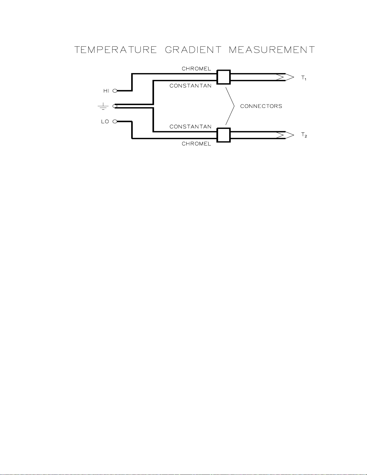
The air temperature gradient is measured with fine wire chromel–constantan thermocouples. The thermocouples are wired into the datalogger such that the temperature gradient is measured differentially (Figure 1.2-2). The differential voltage is due to the difference in

temperature between T

and T2 and has no

inherent sensor offset error. The datalogger resolution is 0.006°C with 0.1 µV rms noise.

The thermocouples are not aspirated. Calculations indicate that a 25 µm (0.001 in) diameter thermocouple experiences less than

-1

0.2°C and 0.1°C heating at 0.1 m s

-1

1 m s W m

wind speeds, respectively, under 1000

-2

solar radiation (Tanner, 1979). More

and

importantly, error in the gradient measurement is due only to the difference in the radiative heating of the two thermocouple junctions. The physical symmetry of the thermocouple junction minimizes this error. Conversely, contamination of only one junction can cause large errors. A pair of 76 µm (0.003 in) thermocouples with two parallel junctions at each height are used to make the temperature gradient measurement

Applying temperature gradients to the thermocouple connectors was found to cause offsets. The connector mounts were designed with radiation shields and thermal conductors to minimize gradients.

1.2.3 NET RADIATION AND SOIL HEAT FLUX

Net radiation and soil heat flux are averaged over the same time period as the water vapor, temperature, and carbon dioxide gradient.

To measure soil heat flux, heat flux plates are buried in the soil at a depth of eight centimeters. The average temperature of the soil layer above the plate is measured using four parallel thermocouples. The heat flux at the surface is

1-3

SECTION 1. SYSTEM OVERVIEW

then calculated by adding the heat flux measured by the plate to the energy stored in the soil layer. The storage term is calculated by multiplying the change in soil temperature over the averaging period by the soil heat capacity.

1.2.4. POWER SUPPLY

The current requirements of the components of the 023/CO2 Bowen Ratio system are given in Table 1.2-1.

TABLE 1.2-1. Component Power

Requirements

CURRENT

COMPONENT at 12 VDC

LI-6262 1000 mA

Pump 60 mA

CR23X 5 mA

Two large solar panels (60 watts or greater) and a 70 amp-hour battery are capable of providing a continuous current of 1.1 A, assuming 1000

-2

of incoming solar radiation for 12 hours a

Wm day. The solar panels are required to keep a full charge on the battery. The voltage of the battery must be monitored by the station operator. Do not allow the battery voltage to fall below 11 VDC. If the battery voltage falls below 11 VDC, the IRGA will shut down. The station operator must then manually reset the IRGA by turning the power switch (on the front panel) off and then on. A datalogger control port is used to control power to the pump via relays.

1-4

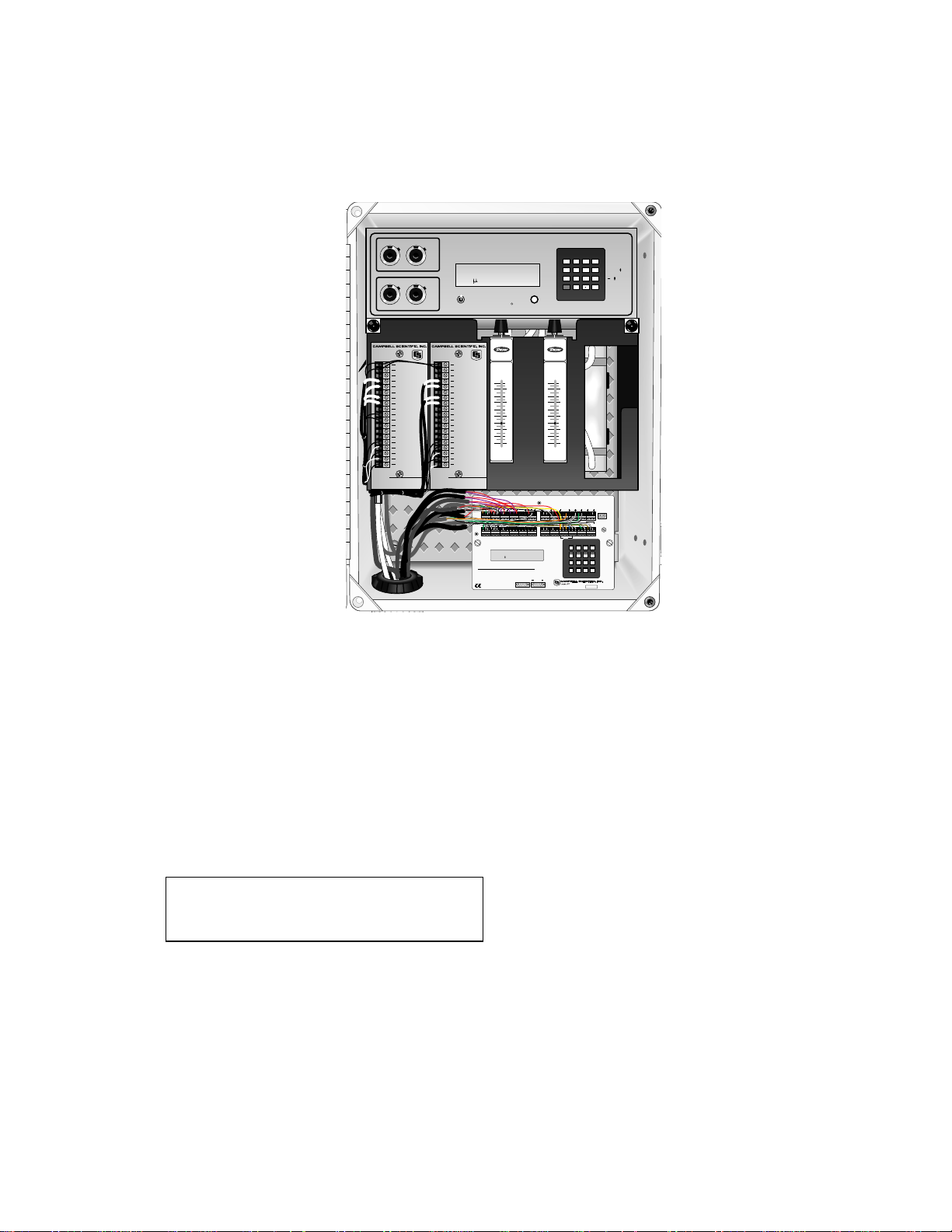
SECTION 2. LI-6262 INSTALLATION

This section describes how the LI-6262 Infrared Gas Analyzer is integrated into the 023/CO2 enclosure.

ZERO SPAN

0 0

CO /

H O

H O ANALYZER

Model LI-6262

C2C2mV

m/m

LI-COR

339.48

-5.250

123

FUNCTION

456

EXIT

789

ENTER

READYOFF

+12V GROUND GROUND SOL 1+ SOL 1GROUND SOL 2+ SOL 2GROUND PUMP+ PUMPGROUND MIRROR+ MIRRORGROUND SOL 1 CTRL SOL 2 CTRL M&P OFF M&P ON

BR RELAY DRIVER-12V

MADE IN USA

FIGURE 2-1. 023/CO2 Bowen Ratio System

2.1 ANALYZER PREPARATION

The LI-6262 has two inline Balston filters inside the analyzer, ahead of the reference and sample cells. These filters have high flow rates with low back pressure. However, they have a time constant of about a minute. To decrease the time constant of the analyzer, replace the Balston filters with tubing. The ACRO50 filters installed on the Bowen Ratio arms will provide sufficient filtration for the LI-6262. Section 7.5 of the LI-6262 manual provides more information on removing the Balston filters.

CAUTION: Never operate the LI-6262 without adequate filtration ahead of the reference and sample cells.

2.2 INITIAL SETUP

The LI-6262 is mounted on top of the black bracket inside the 023/CO2 enclosure. It is held in place by two mounting rails that are attached to the bottom of the analyzer by four pan head screws (Figure 2.2-1). It may be necessary to relocate the rubber feet of the LI-6262 so they do not interfere with the black mounting bracket.

MADE IN USA

+12V GROUND GROUND SOL 1+ SOL 1GROUND SOL 2+ SOL 2GROUND PUMP+ PUMPGROUND MIRROR+ MIRRORGROUND SOL 1 CTRL SOL 2 CTRL M&P OFF M&P ON

BR RELAY DRIVER-12V

CC / MIN.

AIR

X 100

REFERENCEREFERENCE

910

DIFF

13 14

15 16

17 18

19 20

21 22

DIFF

04:REF_TEMP +21.93

CR23X MICROLOGGER

CS I/O

CC / MIN.

AIR

X 100

SAMPLESAMPLE

11 12

EX1

EX2

EX3

EX4

CAO1

CAO2P1P2P3P4

23 24

COMPUTER

RS232

POWER OUT CONTROL I/O

G5VG

SW12G12V

12VGC1C2C3C4GC5C6C7C8

SDM

1 2 3 A

4 5 6 B

7 8 9 C

0 # D

G 12V

POWER IN

GROUND

LUG

SN:

MADE IN USA

The 023/CO2 Bowen Ratio system requires that the LI-6262 operate in differential mode (see the LI-6262 manual for details). In this mode carbon dioxide and water vapor are scrubbed on the chopper input.

Prepare a soda lime and desiccant tube, as described in Section 7.4 of the LI-6262 manual. The bevaline tube that connects the soda lime and desiccant tube to the LI-6262 chopper must be replaced with longer tubes, to accommodate mounting the desiccant tube to the enclosure backplate. Attach the bottom hose (nearest the soda lime) to the FROM CHOPPER fitting and the top hose (nearest the perchlorate) to the TO CHOPPER fitting (Figure 2.2-2). Install the tube in the enclosure using the two clips mounted on the left side of the backplate.

Every hour the sample cell of the analyzer is scrubbed of carbon dioxide and water vapor with external soda lime and desiccant tubes. The absolute concentration of carbon dioxide and water vapor is then measured by the analyzer. The soda lime and desiccant tubes are plumbed in series and are integrated into

2-1

SECTION 2. LI-6262 INSTALLATION

H O

CO /2H O2ANALYZER

Model LI-6262

LI-COR

OFF

FUNCTION EEX

ENTER

CC / MIN.

AIR

X 100

CC / MIN.

AIR

X 100

REFERENCE SAMPLE

+12V GROUND GROUND SOL 1+ SOL 1GROUND SOL 2+ SOL 2GROUND PUMP + PUMP GROUND MIRROR + MIRROR GROUND SOL 1 CTRL SOL 2 CTRL M&P OFF M&P ON

BR RELAY DRIVER -12V

MADE IN USA

+12V GROUND GROUND SOL 1+ SOL 1GROUND SOL 2+ SOL 2GROUND PUMP + PUMP GROUND MIRROR + MIRROR GROUND SOL 1 CTRL SOL 2 CTRL M&P OFF M&P ON

BR RELAY DRIVER -12V

MADE IN USA

123A 456B 789C

0#D

1 2 3 4 5 6 7 8

9 10 11 12 13 14 15 16

DAC1 5V DAC1 100mV DAC1 20mA SIG GND DAC2 5V DAC2 100mV DAC2 20mV SIG GND CO 1S

H O 1S

TEMP 5V SIG GND AUX INPUT CHASSIS GND

CO 4S

H O 4S

115

RS-232C DCE SAMPLE REFERENCE

OUT

SCRUBBER TO

CHOPPER

VOLTAGE

.25A/230V

.5A/115V

FROM CHOPPER

10.5-16 VDC

UNPLUG AC POWER BEFORE SERVICING TO PREVENT PERSONAL INJURY

WARNING!

LI-6262

CO /H O ANALYZER

MODEL SR. NO.

LI-COR

U.S. Patent # 4,803,370

U.S. and Foreign Patents Pending

Made in U.S.A.

IRG3-2 2 9

LI-6262 Maintenance

Internal soda Lime/Desiccant must be changed annually.

A range of time periods are given for maintenance. Actual time period depends on operating conditions.

External Soda Lime/Desiccant: weekly, monthly Internal Air Filters: monthly, yearly Fan Air Filter: weekly, monthly Factory Checkout: yearly

See operator's maunal for servicing Internal components.

the system with a pair of quick connect connectors.

Fill the tube with the female connector with soda lime and the tube with the male connector with magnesium perchlorate. Plumb the tubes as shown in Figure 2.2-3. The tubes are attached to the backplate with two pair of clips.

The analyzer's analog output is connected to the CR23X datalogger with the 023/CO2 signal cable. Table 2.2-1 describes the connections on the analyzer end of the signal cable. Table

3.3-1 (Section 3) describes the connections on the CR23X end of the cable.

TABLE 2.2-1. LI-6262 Analog Output

Connections

COLOR CONNECTION

CHANNEL BLACK SIG GND 8 GREEN CO2 0.1 SEC 9 WHITE H2O 0.1 SEC 11 RED TEMP 5V 13 CLEAR CHASSIS GND 16

After the analyzer is plumbed and wired into the 023/CO2 system and the mounting rails are fastened to the analyzer, slide the analyzer over the black bracket as shown in Figure 2.2-1. Line the push buttons with the holes on either side of the bracket and press firmly until the analyzer is seated on the bracket. Push the buttons in until a click is heard and LI-6262 is securely attached to the black bracket.

NOTE: The analyzer fits snugly within the fiberglass enclosure. The zero and span knobs will make contact with the inside of the enclosure lid. With time, four black rings will appear on the lid. The zero and span knobs are not exposed to any excessive stress when the lid is closed and latched.

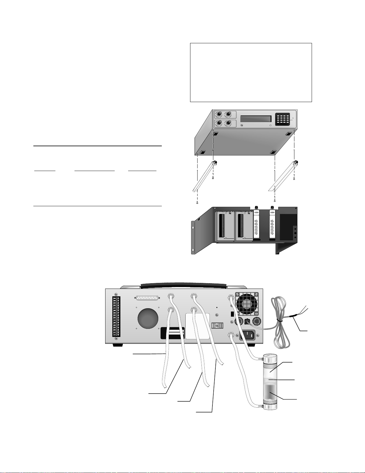
FIGURE 2.2-1. LI-6262 and Mounting

Hardware

2-2

To Sample Flowmeter

To Valve B

To Reference Flowmeter

To Zero Switch

FIGURE 2.2-2. Plumbing Inputs

Mount on Back Plate

To 12 VDC 70 Ahr (or greater) Battery

Magnesium Perchlorate

Fiberglass Wool

Soda Lime

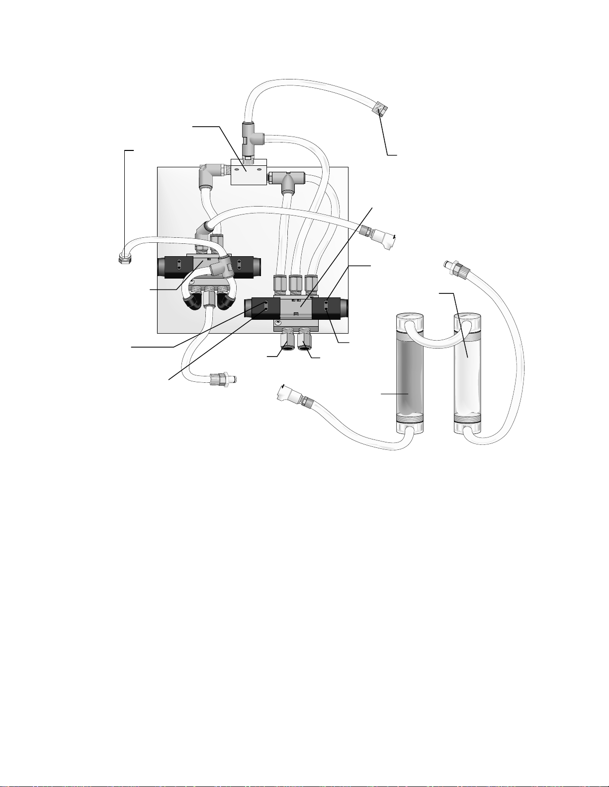
Zero Switch

SECTION 2. LI-6262 INSTALLATION

Valve B

SOL 2-

To Sample In

SOL 2+

Upper Arm

To Reference In

Valve A

SOL 1-

Magnesium Perchlorate

SOL 1+

Lower Arm

Soda Lime

CO2PUMB (system)

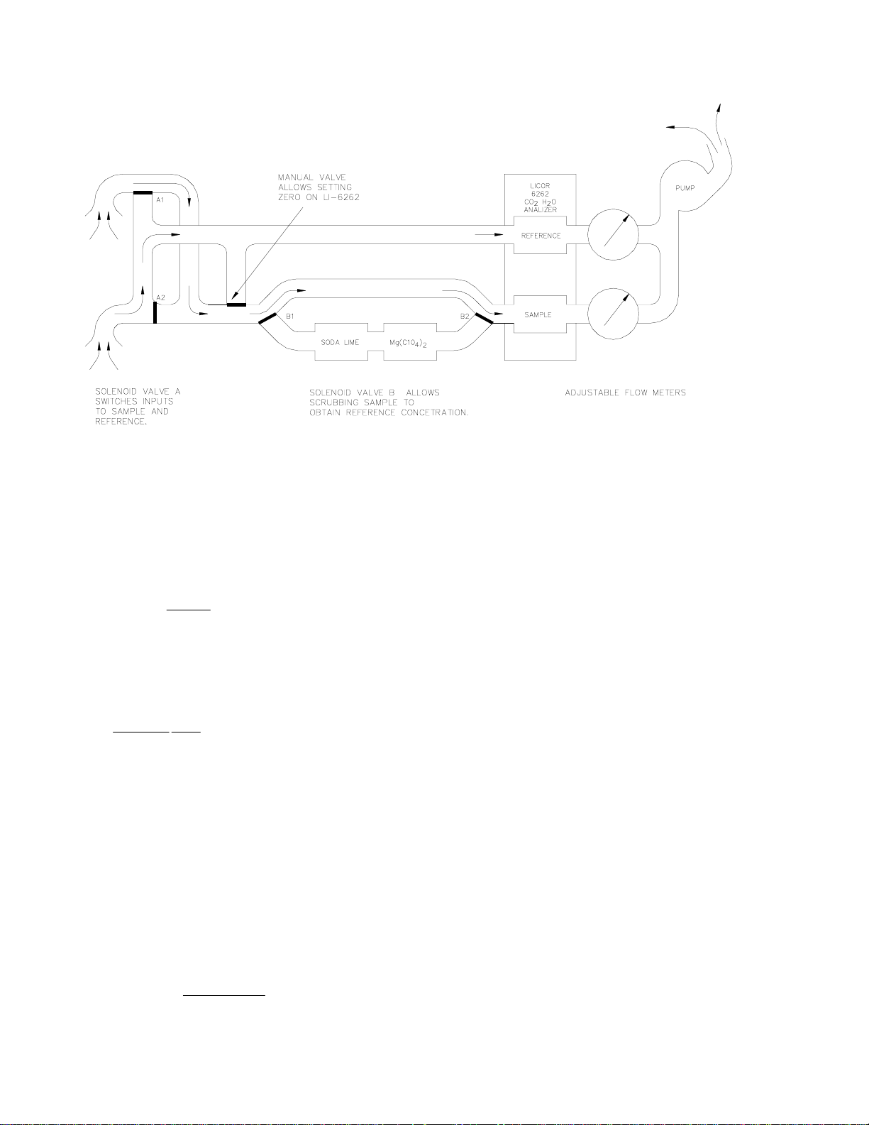
FIGURE 2.2-3. 023/CO2 Plumbing, Valves, and Soda Lime and Desiccant Tubes

2-3

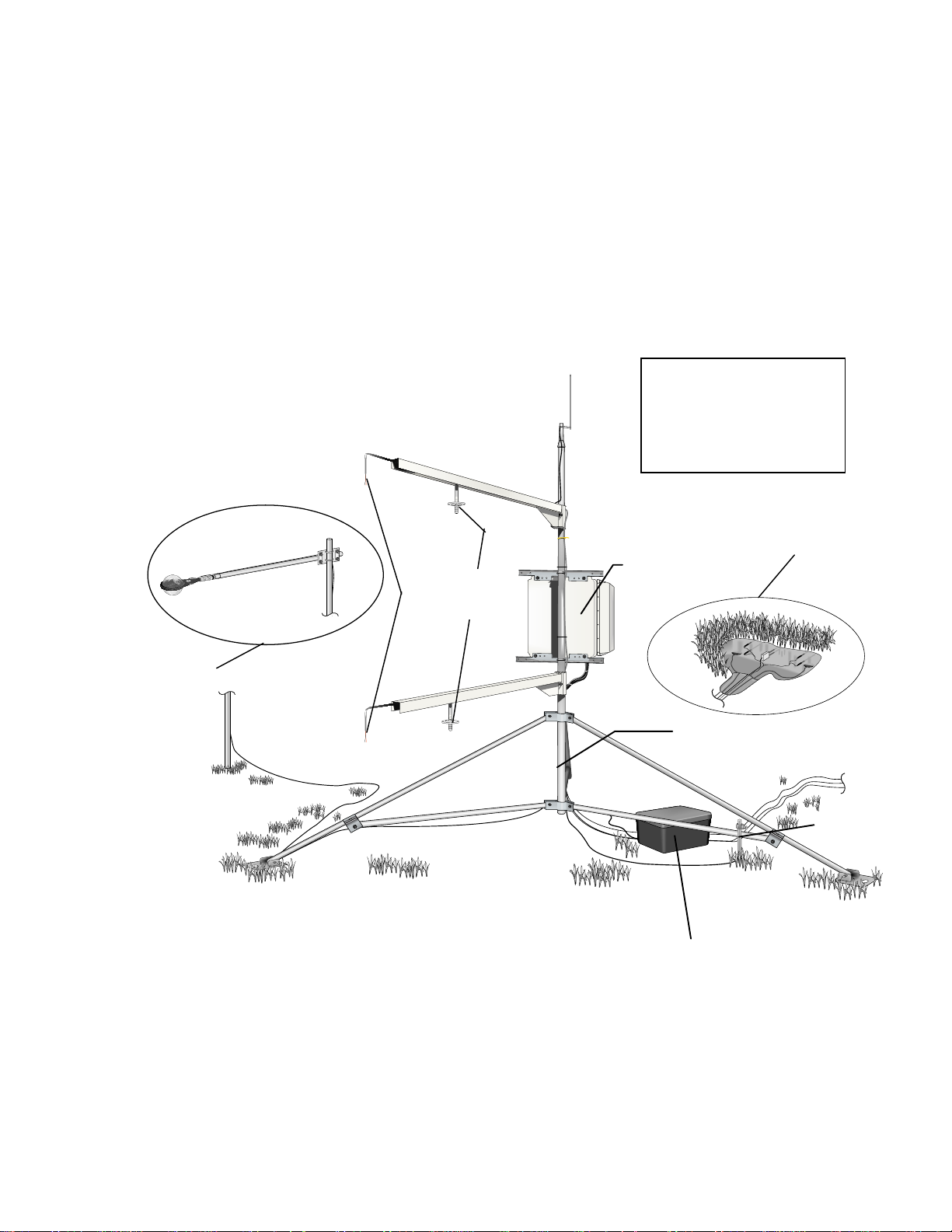
SECTION 3. STATION INSTALLATION

ers

Figure 3-1 shows the typical 023/CO2 system installed on a CM10 tripod. The 023/CO2 enclosure and mounting arms mount to the tripod mast (1 1/2 in. pipe) with U-bolts. The size of the tripod allows the heights of the arms to be adjusted from 0.5 to 3 meters. The mounting arms should be oriented due south to avoid partial shading of the thermocouples.

Two solar panels (60 watts or greater) are mounted on a separate tripod or A-frame (not provided by Campbell Scientific). The net radiometer is mounted on a separate stake (not provided by Campbell Scientific). It should be positioned so that it is never shaded by the tripod and mounting hardware, and such that the mounting hardware is not a significant portion of its field of view.

Other Sensors Not Shown: (1) Wind Speed and Direction

Sensor

(1) Air Temperature and

Humidity Sensor

BOWENCO2 (system)

Intake Filt

023/CO2 Enclosure

Type E Fine Wire Thermocouples

Averaging Soil Temperature Probe and Soil Heat Flux Plates

Net Radiometer

CM10 Tripod

Grounding Rod

User Supplied deep cycle battery (70 AHr or greater). Two Solar Panels, 60 watts or greater (not shown).

FIGURE 3-1. 023/CO2 Bowen Ratio System with CO2 Flux

3-1

SECTION 3. STATION INSTALLATION

3.1 SENSOR HEIGHT AND SEPARATION

There are several factors which must be balanced against each other when determining the height at which to mount the support arms for the thermocouples and air intakes.

The differences in moisture, temperature, and carbon dioxide increase with height, thus the resolution of the gradient measurements improves with increased separation of the arms.

The upper mounting arm must be low enough that it is not sampling air that is coming from a different environment up wind. The air that the sensors see must be representative of the soil/vegetation that is being measured. As a rule of thumb, the surface being measured should extend a distance upwind that is at least 100 times the height of the sensors. The following references discuss fetch requirements in detail: Brutsaert (1982); Dyer and Pruitt (1962); Gash (1986); Schuepp, et al. (1990); and Shuttleworth (1992).

The lower mounting arm needs to be higher than the surrounding vegetation so that the air it is sampling is representative of the bulk crop surface, and not a smaller surface i.e. do not place the lower arms in between the rows of a row crop like sorghum.

The example SPLIT parameter file that calculates the surface fluxes assumes a 1.0 meter arm separation. If your station is installed with an arm separation other than 1.0 meter, measure and note the separation. Be sure to change the arm separation, DZ, in the SPLIT parameter file CALBRC.PAR.

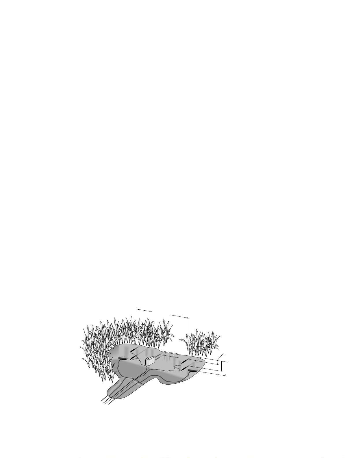
3.2 SOIL THERMOCOUPLES AND HEAT FLUX PLATES

The soil thermocouples and heat flux plates are installed as shown in Figure 3.2-1. The TCAV parallels four thermocouples together to provide the average temperature, see Figure 3.2-2. It is constructed so that two thermocouples can be used to obtain the average temperature of the soil layer above one heat flux plate and the other two above the second plate. The thermocouple pairs may be up to two meters apart.

The location of the two heat flux plates and thermocouples should be chosen to be representative of the area under study. If the ground cover is extremely varied, it may be necessary to have additional sensors to provide a valid average.

Use a small shovel to make a vertical slice in the soil and excavate the soil to one side of the slice. Keep this soil intact so that it can be replaced with minimal disruption.

The sensors are installed in the undisturbed face of the hole. Measure the sensor depths from the top of the hole. Make a horizontal cut eight cm below the surface with a knife into the undisturbed face of the hole and insert the heat flux plate into the horizontal cut. Press the stainless steel tubes of the TCAVs above the plates as shown in Figure 3.2-1. When removing the thermocouples, grip the tubing, not the thermocouple wire.

Install the CS615 as shown in Figure 3.2-1. See the CS615 manual (Section 5) for detailed installation instructions.

3-2

Up to 1 m

2.5 cm

Partial emplacement of the HFT3 and the TCAV sensors is shown for illustration purposes. All sensors must be completely inserted into the soil face before the hole is backfilled.

6 cm

2 cm

Ground Surface

8 cm

FIGURE 3.2-1. Placement of Thermocouples and Heat Flux Plates

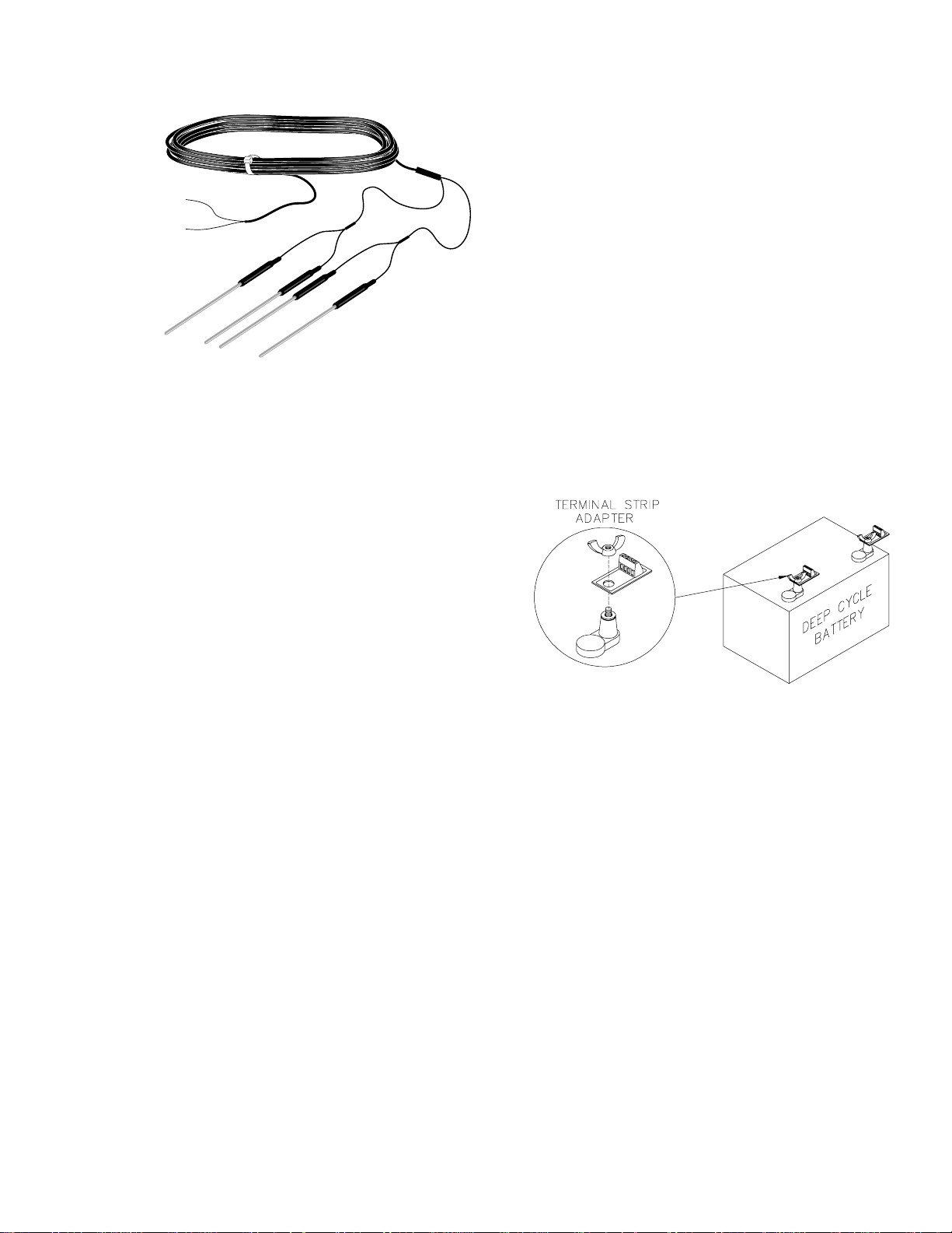
FIGURE 3.2-2. TCAV Spatial Averaging

Thermocouple Probe

Never run the leads directly to the surface. Rather, bury the sensor leads a short distance back from the hole to minimized thermal conduction on the lead wires. Replace the excavated soil back into its original position after the TCAVs are installed.

SECTION 3. STATION INSTALLATION

3.4 BATTERY CONNECTIONS

Two terminal strip adapters for the battery posts (P/N 4386) are provided with the 023/CO2 (Figure 3.4-1). These terminal strips will mount to the wing nut battery posts on most deep cycle lead acid batteries.

The solar panels (60 watts or greater), BR relay driver, LI-6262, and CR23X each have separate power cables. Once the system is installed, these power cables are then connected to the external battery (red to positive, black to negative). The CR23X power cable is shipped in the 023/CO2 enclosure and must be connected to the +12V (red from power cable) and ground (black from power cable) terminals on the CR23X wiring panel.

Several deep cycle batteries can be connected in parallel, to provide power to the system during cloudy or overcast days.

Finally, wrap the thermocouple wire around the CR23X base at least twice before wiring them into the terminal strip. This will minimized thermal conduction into the terminal strip. After all the connections are made, replace the terminal strip cover.

3.3 WIRING

Table 3.3-1 lists the connections to the CR23X for the standard 023/CO2 system using the example program in Section 4. Because the air temperature measurements are so critical, the air temperature thermocouples are connected to channel 4 (the channel that is closest to the reference temperature thermistor). The input terminal strip cover for the CR23X must be installed once all connections have been made and verified (Section 13.4.1 of the CR23X manual).

FIGURE 3.4-1. Terminal Strip Adapters for

Connections to Battery

The LI-6262 can not be turned on and off with relays without a hardware modification to the power board (contact LI-COR for details). After the hardware modification has been made. A Crydom D1D07 (P/N 7321) can be used to power the LI-6262. The control side of the D1D07 can be operated by a BR relay driver. Do not power the LI-6262 through the BR relay driver, because there is a 0.8 V drop through it and the high current drain of the LI-6262 may create an offset in single ended measurements.

3-3

SECTION 3. STATION INSTALLATION

TABLE 3.3-1. CR23X/Sensor Connections for Example Program

CHANNEL SENSOR COLOR 1H Q7.1 RED

1L Q7.1 BLACK

Q7.1 CLEAR

2H CS615 GREEN 2L WIND DIRECTION RED

CS615 BLACK/CLEAR WIND DIRECTION WHITE/CLEAR

3H TCAV PURPLE 3L TCAV RED

TCAV CLEAR

4H UPPER 0.003 TC - CHROMEL PURPLE 4L LOWER 0.003 TC - CHROMEL PURPLE

AIR TEMP TCs - CONSTANTAN RED/RED

5H HFT3 #1 BLACK 5L HFT3 #1 WHITE

HFT3 #1 CLEAR

6H HFT3 #2 BLACK 6L HFT3 #2 WHITE

HFT3 #3 CLEAR

7H LI-6262 (CO2 0.1 Second) GREEN 7L LI-6262 (Signal low) BLACK

8H LI-6262 (H2O 0.1 Second) WHITE 8L LI-6262 (Jumper to 6L) BLACK

9H LI-6262 (Analyzer Temperature) RED 9L LI-6262 (Jumper to 7L) BLACK

LI-6262 (Ground) CLEAR

10H HMP45C (Temperature) YELLOW 10L HMP45C PURPLE

CLEAR

11H HMP45C (Relative Humidity) BLUE 11L JUMPER TO 10L JUMPER TO 10L

P1 WIND SPEED BLACK GND WIND SPEED WHITE/CLEAR EX2 WIND DIRECTION BLACK +12 V CS615 RED

+12 V HMP45C RED G HMP45C BLACK +5 V HMP45C ORANGE

C1 PULSE FOR LOWER ARM TO REFERENCE

AND UPPER ARM TO SAMPLE ORANGE w/ WHITE

C2 PULSE FOR UPPER ARM TO REFERENCE

AND LOWER ARM TO SAMPLE BLUE w/ WHITE C3 PULSE TO END SCRUB WHITE w/ ORANGE C4 PULSE TO SCRUB WHITE w/ BLUE

3-4

SECTION 3. STATION INSTALLATION

C5 PULSE TO TURN ON PUMP GREEN w/ WHITE

(SET FLAG 5 AND 6; RESET FLAG 5) WHITE w/ GREEN

C6 PULSE TO TURN OFF PUMP BROWN w/ WHITE

(SET FLAG 5; RESET FLAG 6 AND 5) WHITE w/ BROWN C7 CS615 (Control) ORANGE G GROUND WIRE CLEAR

3-5

SECTION 4. SAMPLE 023/CO2 PROGRAM

4.1 PROGRAM DETAILS

4.1.1 SCRUBBING THE SAMPLE CELL

The signal from the analyzer is proportional to the difference in concentration between the reference and sample cells. If the reference concentration, C concentration in the sample cell can be found using the relationship below,



CVGV

f (15)

()





where the function f is a fifth order polynomial of the form

=+ + + + (16)

f(V) AV BV CV DV EV

with coefficients A, B, C, D, and E that are unique to each analyzer, C concentration in the sample cell, V is the analyzer output, V analyzer if there was zero concentration in the reference cell and a known concentration, C the sample cell, T and T temperature and calibration temperature, P and

are the ambient and calibration (sea level)

pressures, and G is given by:

−

where K is a calibration constant. Every hour the sample cell is scrubbed of

carbon dioxide and water vapor. The absolute concentration of carbon dioxide and water vapor can then be calculated. Scrubbing the sample cell and leaving the reference cell at ambient avoids the zero offset shift that occurs when the concentration in the reference cell changes.

The equations presented in the LI-6262 manual are for the case when the concentration in the reference cell is known (scrubbed) and the concentration in sample cell is unknown. Since the 023/CO2 system scrubs the sample cell, the equations must be reformulated.

When the sample cell is scrubbed the concentration C the following is true,

+=0 (18)

VG V

, is known, the absolute







2345

is the gas

is the signal output from the

are the analyzer

in Eq. (13) is equal to zero and

, in

(17)

VVG

=− . (19)

Substituting Eq. (17) into (15) and solving for G yields the relationship below.

−

Now substitute Eq. (18) into (17).

=−

−

is the signal the analyzer would output if the reference cell was scrubbed instead of the sample cell. The value found from Equation (21) is used in the fifth order polynomial to find the absolute concentration of carbon dioxide and water vapor. New values of V

and G are

calculated every hour and used in measuring the carbon dioxide and water vapor gradient.

The absolute concentration of water vapor and carbon dioxide are not corrected for T/To online. Thus, during a scrub, the absolute concentrations displayed by the LI-6262 will differ by a factor of T/To to those calculated by the CR23X.

4.1.2 COEFFICIENTS

The unique calibration coefficients for the LI-6262 must be entered in the CR23X program. The calibration temperature (Kelvins) and K coefficients are entered in Subroutine 1. The polynomial coefficients A (C1), B (C2), C (C3), D (C4), and E (C5) are entered in Subroutine 7.

The magnitude of the coefficients that can be entered into the polynomial instruction (Instruction 55) is 0.00001 to 99999. Since the coefficients are outside this range, they must be prescaled. The input to the polynomial is

-3

multiplied by 10

by the first instruction in Subroutine 7. The coefficients, as they are given by LI-COR, must be transformed in order to enter them into the program. To perform the carbon dioxide and water vapor coefficient transformation; multiply the A (C1) coefficient by

, the B (C2) coefficient by 106, the C (C3)

10 coefficient by 10

, and the E (C5) coefficient by 1015. Table

, the D (C4) coefficient by

4.1-1 provides and example of how to transform typical LI-6262 water vapor coefficients.

(20)

(21)

4-1

SECTION 4. SAMPLE 023/CO2 PROGRAM

TABLE 4.1-1. Example LI-6262 Carbon Dioxide Coefficients

Coefficient Coefficient

(LI-COR) LI-6262

A 0.15053 10

B 7.0875 x 10 C 8.4794 x 10 D -1.1482 x 10 E 7.5212 x 10

-6

-9

-12

-17

Multiply by CR23X (CSI)

10 10 10

3 6

9 12 15

150.53 C1

7.0875 C2

8.4794 C3

-1.1482 C4

0.07512 C5

4.2 CR23X PROGRAM

A copy of the example program for the CR23X is available on the Campbell Scientific ftp site at ftp://ftp.campbellsci.com/pub/outgoing/files/br_co2.exe. Br_co2.exe is a self extracting file. At a DOS prompt, type in br_co2.exe and press the <enter> key. Use EDLOG to edit the example program. Table

4.2-2 lists the outputs from the example program.

TABLE 4.2-1. Example Datalogger Program

;{CR23X} ; ;c:\dl\co2\co2feb98.csi ;23 February 1998

;Example CR23X program for the 023/CO2 Bowen ratio system w/ CO2 Flux. ;Flag 1 - When HIGH stops averaging during scrubbing or manual

; control of flow valves. When LOW Subroutine 1 loads ; constants. ;Flag 2 - When HIGH the upper arm is routed into the sample input ; and the lower arm into the reference, when LOW the ; upper arm is routed into the reference and the lower ; arm into the sample. ;Flag 3 - When HIGH timing out for forty seconds after switching ; upper and lower levels. ;Flag 4 - Is set HIGH during automatic and manual scrub. ;Flag 5 - When HIGH allows manual control of flow valves and turning ; the pump on and off. Use Flag 2 to toggle the valve ; and Flag 6 to operate the pump. ;Flag 6 - When HIGH the pump is on, When LOW the pump is off. ;Flag 7 - Used in Subroutine 7 to determine which polynomial to use. ;Flag 8 - Set HIGH to perform a manual scrub.

*Table 1 Program

01: 1 Execution Interval (seconds)

;Make measurements.

01: Internal Temperature (P17)

1: 35 Loc [ refrnc ]

4-2

02: Thermocouple Temp (SE) (P13)

1: 1 Reps 2: 21 10 mV, 60 Hz Reject, Slow Range 3: 8 In Chan 4: 2 Type E (Chromel-Constantan) 5: 35 Ref Temp Loc [ refrnc ] 6: 33 Loc [ lwr_TC ] 7: 1 Mult 8: 0 Offset

03: Thermocouple Temp (Diff) (P14)

1: 1 Reps 2: 21 10 mV, 60 Hz Reject, Slow Range 3: 4 In Chan 4: 2 Type E (Chromel-Constantan) 5: 33 Ref Temp Loc [ lwr_TC ] 6: 32 Loc [ upr_TC ] 7: 1 Mult 8: 0 Offset

04: Z=X-Y (P35)

1: 33 X Loc [ lwr_TC ] 2: 32 Y Loc [ upr_TC ] 3: 34 Z Loc [ del_TC ]

SECTION 4. SAMPLE 023/CO2 PROGRAM

05: If Flag/Port (P91)

1: 24 Do if Flag 4 is Low 2: 30 Then Do

06: Volt (Diff) (P2)

1: 2 Reps 2: 24 1000 mV, 60 Hz Reject, Slow Range 3: 7 In Chan 4: 10 Loc [ co2mV ] 5: 1 Mult 6: 0 Offset

07: If (X<=>F) (P89)

1: 10 X Loc [ co2mV ] 2: 4 < 3: -500 F 4: 30 Then Do

08: Volt (Diff) (P2)

1: 1 Reps 2: 25 5000 mV, 60 Hz Reject, Fast Range 3: 7 In Chan 4: 10 Loc [ co2mV ] 5: 1 Mult 6: 0 Offset

09: End (P95)

;Compute CO2 and H2O gradient. ;

10: Do (P86)

1: 3 Call Subroutine 3

;Analyzer Temperature

4-3

SECTION 4. SAMPLE 023/CO2 PROGRAM

11: Do (P86)

1: 27 Set Flag 7 Low

12: Beginning of Loop (P87)

1: 0 Delay 2: 2 Loop Count

13: Z=X*Y (P36)

1: 10-- X Loc [ co2mV ] 2: 26-- Y Loc [ G_co2 ] 3: 41-- Z Loc [ co2mVinpt ]

14: Z=X+Y (P33)

1: 41-- X Loc [ co2mVinpt ] 2: 24-- Y Loc [ Vr_co2_mV ] 3: 41-- Z Loc [ co2mVinpt ]

15: Do (P86)

1: 7 Call Subroutine 7

16: Z=X-Y (P35)

1: 28-- X Loc [ co2_uM ] 2: 21-- Y Loc [ co2ref_uM ] 3: 30-- Z Loc [ del_co2 ]

;Apply Polynomial

17: Z=X*Y (P36)

1: 30-- X Loc [ del_co2 ] 2: 18-- Y Loc [ Ta_To_co2 ] 3: 30-- Z Loc [ del_co2 ]

18: Do (P86)

1: 17 Set Flag 7 High 19: End (P95) 20: Do (P86)

1: 8 Call Subroutine 8 21: Else (P94) 22: Do (P86)

1: 1 Call Subroutine 1 23: End (P95)

;If valves have just switched or the ;system is in manual control (Flag 5 High) ;set Flag 9 High. ;

24: If Flag/Port (P91)

1: 11 Do if Flag 1 is High

2: 30 Then Do

;Move values and change sign

;Scrub

25: Do (P86)

1: 19 Set Flag 9 High

4-4

26: Else (P94) 27: If Flag/Port (P91)

1: 13 Do if Flag 3 is High 2: 19 Set Flag 9 High

28: End (P95)

;Generate gradient output array every twenty minutes. ;

29: If time is (P92)

1: 0 Minutes into a 2: 20 Minute Interval 3: 10 Set Output Flag High

30: Set Active Storage Area (P80)

1: 1 Final Storage 2: 21 Array ID

31: Real Time (P77)

1: 1110 Year,Day,Hour/Minute

32: Resolution (P78)

1: 1 high resolution

SECTION 4. SAMPLE 023/CO2 PROGRAM

33: Average (P71)

1: 5 Reps 2: 36 Loc [ co2mVcorr ]

34: Sample (P70)

1: 7 Reps 2: 21 Loc [ co2ref_uM ]

35: Do (P86)

1: 29 Set Flag 9 Low

36: Average (P71)

1: 3 Reps 2: 33 Loc [ lwr_TC ]

37: Sample (P70)

1: 2 Reps 2: 62 Loc [ scb_Tao_C ]

38: If Flag/Port (P91)

1: 15 Do if Flag 5 is High 2: 30 Then Do

39: Do (P86)

1: 2 Call Subroutine 2

;Manual valve control

40: Else (P94)

4-5

SECTION 4. SAMPLE 023/CO2 PROGRAM

;Perform an automatic scrub at the top of ;the hour. ;

41: If time is (P92)

1: 0 Minutes into a

2: 60 Minute Interval

3: 14 Set Flag 4 High 42: If Flag/Port (P91)

1: 18 Do if Flag 8 is High

2: 14 Set Flag 4 High

;Synchronize valve switching every four ;minutes. ;

43: If time is (P92)

1: 0 Minutes into a

2: 4 Minute Interval

3: 30 Then Do 44: Do (P86)

1: 21 Set Flag 1 Low 45: Do (P86)

1: 42 Set Port 2 High 46: Do (P86)

1: 22 Set Flag 2 Low 47: Do (P86)

1: 13 Set Flag 3 High 48: Do (P86)

1: 9 Call Subroutine 9 49: End (P95) 50: If time is (P92)

1: 2 Minutes into a

2: 4 Minute Interval

3: 30 Then Do 51: Do (P86)

1: 41 Set Port 1 High 52: Do (P86)

1: 12 Set Flag 2 High 53: Do (P86)

1: 13 Set Flag 3 High

;Set all ports LOW

54: Do (P86)

1: 9 Call Subroutine 9 55: End (P95)

4-6

;Set all ports LOW

SECTION 4. SAMPLE 023/CO2 PROGRAM

56: If time is (P92)

1: 40-- Minutes (Seconds --) into a 2: 60 Interval (same units as above)

3: 23 Set Flag 3 Low 57: End (P95) 58: Serial Out (P96)

1: 71 SM192/SM716/CSM1

*Table 2 Program

01: 10 Execution Interval (seconds)

01: Batt Voltage (P10)

1: 9 Loc [ battry ] 02: Volt (Diff) (P2)

1: 1 Reps

2: 24 1000 mV, 60 Hz Reject, Slow Range

3: 10 DIFF Channel

4: 1 Loc [ HMP_T ]

5: .1 Mult

6: -40 Offset 03: Volt (Diff) (P2)

1: 1 Reps

2: 24 1000 mV, 60 Hz Reject, Slow Range

3: 11 DIFF Channel

4: 8 Loc [ rh_frac ]

5: .001 Mult

6: 0 Offset 04: Saturation Vapor Pressure (P56)

1: 1 Temperature Loc [ HMP_T ]

2: 2 Loc [ HMP_e ] 05: Z=X*Y (P36)

1: 8 X Loc [ rh_frac ]

2: 2 Y Loc [ HMP_e ]

3: 2 Z Loc [ HMP_e ] 06: Z=X/Y (P38)

1: 2 X Loc [ HMP_e ]

2: 23 Y Loc [ P_kPa ]

3: 3 Z Loc [ h2o_mM_M ] 07: Z=X*F (P37)

1: 3 X Loc [ h2o_mM_M ]

2: 1000 F

3: 3 Z Loc [ h2o_mM_M ]

4-7

SECTION 4. SAMPLE 023/CO2 PROGRAM

08: Volt (Diff) (P2)

1: 1 Reps 2: 23 200 mV, 60 Hz Reject, Slow Range 3: 1 DIFF Channel 4: 4 Loc [ Rn ] 5: 1 Mult 6: 0 Offset

09: If (X<=>F) (P89)

1: 4 X Loc [ Rn ] 2: 3 >= 3: 0 F 4: 30 Then Do

;Apply the positive calibration and ;wind speed corrections. ;

10: Do (P86)

1: 4 Call Subroutine 4

11: Else (P94)

;Apply the negative calibration and ;wind speed corrections ;

12: Do (P86)

1: 5 Call Subroutine 5 13: End (P95) 14: Volt (Diff) (P2)

1: 2 Reps

2: 22 50 mV, 60 Hz Reject, Slow Range

3: 5 DIFF Channel

4: 5 Loc [ shf1 ]

5: 1 Mult

6: 0 Offset

;Enter the multiplier for soil heat flux ;number 1 (x.xxx1). ;

15: Z=X*F (P37)

1: 5 X Loc [ shf1 ]

2: 1 F

3: 5 Z Loc [ shf1 ]

;Enter the multiplier for soil heat flux ;number 2 (x.xxx2). ;

16: Z=X*F (P37)

1: 6 X Loc [ shf2 ]

2: 1 F

3: 6 Z Loc [ shf2 ]

;x.xxx1 <- unique value

;x.xxx2 <- unique value

4-8

SECTION 4. SAMPLE 023/CO2 PROGRAM

17: Thermocouple Temp (Diff) (P14)

1: 1 Reps 2: 21 10 mV, 60 Hz Reject, Slow Range 3: 3 In Chan 4: 2 Type E (Chromel-Constantan) 5: 35 Ref Temp Loc [ refrnc ] 6: 7 Loc [ Ts ] 7: 1 Mult 8: 0 Offset

;Turn on CS615 soil moisture probe every twenty minutes. ;

18: If time is (P92)

1: 10 Minutes into a 2: 20 Minute Interval 3: 30 Then Do

19: Do (P86)

1: 47 Set Port 7 High

;Measure CS615 soil moisture probe. When the ;CS615 is off (Control Port 7 low), the values ;in CS615_ms and s_wtr will not change. ;

20: Period Average (SE) (P27)

1: 1 Reps 2: 4 200 kHz Max Freq @ 500 mV Peak to Peak, Period Output 3: 3 SE Channel 4: 10 No. of Cycles 5: 5 Timeout (units = 0.01 seconds) 6: 64 Loc [ cs615_ms ] 7: .001 Mult 8: 0 Offset

;Turn the CS615 off. ;

21: Do (P86)

1: 57 Set Port 7 Low

;Apply the CS615 calibration for a soil ;with an electrical conductivity < 1.0 dS/m. ;See Section 9 of the CS615 manual for ;more information. ;

22: Polynomial (P55)

1: 1 Reps 2: 64 X Loc [ cs615_ms ] 3: 67 F(X) Loc [ s_wtr ] 4: -.187 C0 5: .037 C1 6: .335 C2 7: 0 C3 8: 0 C4 9: 0 C5

4-9

SECTION 4. SAMPLE 023/CO2 PROGRAM

23: Z=X (P31)

1: 64 X Loc [ cs615_ms ]

2: 68 Z Loc [ cs615_mso ] 24: Z=X (P31)

1: 67 X Loc [ s_wtr ]

2: 69 Z Loc [ s_wtr_o ] 25: End (P95) 26: Pulse (P3)

1: 1 Reps

2: 1 Pulse Input Chan

3: 21 Low Level AC, Output Hz

4: 16 Loc [ wnd_spd ]

5: .75 Mult

6: .2 Offset 27: If (X<=>F) (P89)

1: 16 X Loc [ wnd_spd ]

2: 1 =

3: .2 F

4: 30 Then Do 28: Z=F (P30)

1: 0 F

2: 0 Exponent of 10

3: 16 Z Loc [ wnd_spd ] 29: End (P95) 30: AC Half Bridge (P5)

1: 1 Reps

2: 25 5000 mV, 60 Hz Reject, Fast Range

3: 4 In Chan

4: 2 Excite all reps w/Exchan 2

5: 5000 mV Excitation

6: 17 Loc [ wnd_dir ]

7: 355 Mult

8: 0 Offset 31: If time is (P92)

1: 0 Minutes into a

2: 20 Minute Interval

3: 10 Set Output Flag High 32: Set Active Storage Area (P80)

1: 3 Input Storage

2: 13 Loc [ avg_Ts ] 33: Average (P71)

1: 1 Reps

2: 7 Loc [ Ts ] 34: If Flag/Port (P91)

1: 10 Do if Output Flag is High (Flag 0)

2: 30 Then Do

4-10

;Find the change in soil temperature. ;

35: Z=X-Y (P35)

1: 13 X Loc [ avg_Ts ] 2: 12 Y Loc [ prv_Ts ] 3: 14 Z Loc [ del_Ts ]

36: Z=X (P31)

1: 13 X Loc [ avg_Ts ] 2: 12 Z Loc [ prv_Ts ]

;Apply the temperature correction to ;the soil moisture measured by the CS615, ;if the soil temperature is in the range of ;10 degrees C to 30 degrees C. See Section ;4.3.4 of the CS615 manual for more information. ;

37: If (X<=>F) (P89)

1: 13 X Loc [ avg_Ts ] 2: 3 >= 3: 10 F 4: 30 Then Do

SECTION 4. SAMPLE 023/CO2 PROGRAM

38: If (X<=>F) (P89)

1: 13 X Loc [ avg_Ts ] 2: 4 < 3: 30 F 4: 30 Then Do

39: Z=X+F (P34)

1: 13 X Loc [ avg_Ts ] 2: -20 F 3: 65 Z Loc [ D ]

40: Polynomial (P55)

1: 1 Reps 2: 69 X Loc [ s_wtr_o ] 3: 66 F(X) Loc [ E ] 4: -.0346 C0 5: 1.9 C1 6: -4.5 C2 7: 0 C3 8: 0 C4 9: 0 C5

41: Z=X*F (P37)

1: 66 X Loc [ E ] 2: .01 F 3: 66 Z Loc [ E ]

42: Z=X*Y (P36)

1: 65 X Loc [ D ] 2: 66 Y Loc [ E ] 3: 65 Z Loc [ D ]

4-11

SECTION 4. SAMPLE 023/CO2 PROGRAM

43: Z=X-Y (P35)

1: 69 X Loc [ s_wtr_o ]

2: 65 Y Loc [ D ]

3: 70 Z Loc [ s_wtr_o_T ] 44: Else (P94)

;Do not apply temperature correction if the ;soil temperature is outside the range of ;10 degrees C to 30 degrees C. ;

45: Z=X (P31)

1: 69 X Loc [ s_wtr_o ]

2: 70 Z Loc [ s_wtr_o_T ] 46: End (P95) 47: Else (P94)

;Do not apply temperature correction if the ;soil temperature is outside the range of ;10 degrees C to 30 degrees C. ;

48: Z=X (P31)

1: 69 X Loc [ s_wtr_o ]

2: 70 Z Loc [ s_wtr_o_T ] 49: End (P95) 50: End (P95)

;Generate energy balance and meteorological ;output array every twenty minutes. ;

51: If Flag/Port (P91)

1: 10 Do if Output Flag is High (Flag 0)

2: 10 Set Output Flag High 52: Set Active Storage Area (P80)

1: 1 Final Storage

2: 22 Array ID 53: Real Time (P77)

1: 1110 Year,Day,Hour/Minute 54: Resolution (P78)

1: 1 High Resolution 55: Average (P71)

1: 6 Reps

2: 1 Loc [ HMP_T ] 56: Sample (P70)

1: 2 Reps

2: 13 Loc [ avg_Ts ]

4-12

57: Sample (P70)

1: 1 Reps 2: 8 Loc [ rh_frac ]

58: Average (P71)

1: 1 Reps 2: 9 Loc [ battry ]

59: Wind Vector (P69)

1: 1 Reps 2: 60 Samples per Sub-Interval 3: 00 S, qu, & s(qu) Polar 4: 16 Wind Speed/East Loc [ wnd_spd ] 5: 17 Wind Direction/North Loc [ wnd_dir ]

60: Sample (P70)

1: 3 Reps 2: 68 Loc [ cs615_mso ]

*Table 3 Subroutines

SECTION 4. SAMPLE 023/CO2 PROGRAM

;Scrub.

01: Beginning of Subroutine (P85)

1: 1 Subroutine 1

02: If Flag/Port (P91)

1: 21 Do if Flag 1 is Low 2: 30 Then Do

;Enter the CO2 calibration ;temperature (Kelvin). ;

03: Z=F (P30)

1: 1 F 2: 0 Exponent of 10 3: 54 Z Loc [ To_co2 ]

;Enter the H2O calibration ;temperature (Kelvin). ;

04: Z=F (P30)

1: 1 F 2: 0 Exponent of 10 3: 55 Z Loc [ To_h2o ]

;Enter the K coefficient for CO2. ;

05: Z=F (P30)

1: 1 F 2: 0 Exponent of 10 3: 56 Z Loc [ K_co2 ]

;To(CO2) <- unique value

;To(H2O) <- unique value

;K(CO2) <- unique value

4-13

SECTION 4. SAMPLE 023/CO2 PROGRAM

;Enter the K coefficient for H2O. ;

06: Z=F (P30)

1: 1 F

2: 0 Exponent of 10

3: 57 Z Loc [ K_h2o ]

;Enter the local pressure in kPa. ;

07: Z=F (P30)

1: 1 F

2: 0 Exponent of 10

3: 23 Z Loc [ P_kPa ]

;Location 43 = Po/(P*1000) ;

08: Z=F (P30)

1: .10132 F

2: 0 Exponent of 10

3: 43 Z Loc [ Po_P_1000 ] 09: Z=X/Y (P38)

1: 43 X Loc [ Po_P_1000 ]

2: 23 Y Loc [ P_kPa ]

3: 43 Z Loc [ Po_P_1000 ]

;K(H2O) <- unique value

;P(kPa) <- unique value

10: Do (P86)

1: 11 Set Flag 1 High

;During first pass switch the upper arm ;into the reference cell, the lower arm ;into the sample cell, and set the ;scrub valve. ;

11: Do (P86)

1: 42 Set Port 2 High 12: Do (P86)

1: 44 Set Port 4 High 13: Do (P86)

1: 22 Set Flag 2 Low 14: Do (P86)

1: 9 Call Subroutine 9 15: End (P95) 16: Z=Z+1 (P32)

1: 46 Z Loc [ scrub_ctr ]

;Set all ports LOW

4-14

17: Volt (Diff) (P2)

1: 2 Reps 2: 25 5000 mV, 60 Hz Reject, Fast Range 3: 7 In Chan 4: 10 Loc [ co2mV ] 5: 1 Mult 6: 0 Offset

18: Do (P86)

1: 3 Call Subroutine 3

19: If (X<=>F) (P89)

1: 46 X Loc [ scrub_ctr ] 2: 3 >= 3: 50 F 4: 10 Set Output Flag High

20: Set Active Storage Area (P80)

1: 3 Input Storage 2: 10 Loc [ co2mV ]

21: If (X<=>F) (P89)

1: 46 X Loc [ scrub_ctr ] 2: 4 < 3: 40 F 4: 19 Set Flag 9 High

SECTION 4. SAMPLE 023/CO2 PROGRAM

;Analyzer temperature

22: Average (P71)

1: 2 Reps 2: 10 Loc [ co2mV ]

23: Do (P86)

1: 27 Set Flag 7 Low

24: Beginning of Loop (P87)

1: 0 Delay 2: 2 Loop Count

25: Z=X-Y (P35)

1: 56-- X Loc [ K_co2 ] 2: 10-- Y Loc [ co2mV ] 3: 26-- Z Loc [ G_co2 ]

26: Z=X/Y (P38)

1: 56-- X Loc [ K_co2 ] 2: 26-- Y Loc [ G_co2 ] 3: 26-- Z Loc [ G_co2 ]

27: Z=X*Y (P36)

1: 26-- X Loc [ G_co2 ] 2: 10-- Y Loc [ co2mV ] 3: 24-- Z Loc [ Vr_co2_mV ]

28: Z=X*F (P37)

1: 24-- X Loc [ Vr_co2_mV ] 2: -1 F 3: 24-- Z Loc [ Vr_co2_mV ]

4-15

SECTION 4. SAMPLE 023/CO2 PROGRAM

29: Z=X (P31)

1: 24-- X Loc [ Vr_co2_mV ]

2: 41-- Z Loc [ co2mVinpt ] 30: Do (P86)

1: 7 Call Subroutine 7 31: Z=X (P31)

1: 28-- X Loc [ co2_uM ]

2: 21-- Z Loc [ co2ref_uM ] 32: Z=X (P31)

1: 18-- X Loc [ Ta_To_co2 ]

2: 62-- Z Loc [ scb_Tao_C ] 33: Do (P86)

1: 17 Set Flag 7 High 34: End (P95)

;During the autoscrub make one pass ;through the calculation. During a ;manual scrub, pass through the ;calculation until Flag 8 is set Low. ;

35: If Flag/Port (P91)

1: 28 Do if Flag 8 is Low

2: 30 Then Do

;Apply polynomial

36: If Flag/Port (P91)

1: 10 Do if Output Flag is High (Flag 0)

2: 30 Then Do 37: Do (P86)

1: 24 Set Flag 4 Low 38: Z=F (P30)

1: 0 F

2: 0 Exponent of 10

3: 46 Z Loc [ scrub_ctr ] 39: Do (P86)

1: 43 Set Port 3 High 40: Do (P86)

1: 9 Call Subroutine 9 41: End (P95) 42: End (P95) 43: End (P95)

;Manual valve control.

;Set all ports LOW

4-16

44: Beginning of Subroutine (P85)

1: 2 Subroutine 2

45: Do (P86)

1: 11 Set Flag 1 High

46: If Flag/Port (P91)

1: 12 Do if Flag 2 is High 2: 41 Set Port 1 High

47: If Flag/Port (P91)

1: 22 Do if Flag 2 is Low 2: 42 Set Port 2 High

48: If Flag/Port (P91)

1: 16 Do if Flag 6 is High 2: 45 Set Port 5 High

49: If Flag/Port (P91)

1: 26 Do if Flag 6 is Low 2: 46 Set Port 6 High

50: Do (P86)

1: 9 Call Subroutine 9

SECTION 4. SAMPLE 023/CO2 PROGRAM

;Set all ports LOW

51: End (P95)

;Analyzer temperature measurement.

52: Beginning of Subroutine (P85)

1: 3 Subroutine 3

53: Volt (Diff) (P2)

1: 1 Reps 2: 25 5000 mV, 60 Hz Reject, Fast Range 3: 9 In Chan 4: 40 Loc [ T_Anlyzr ] 5: .01221 Mult 6: 0 Offset

54: Z=X+F (P34)

1: 40 X Loc [ T_Anlyzr ] 2: 273.15 F 3: 53 Z Loc [ T_anlyr_K ]

55: Z=X/Y (P38)

1: 53 X Loc [ T_anlyr_K ] 2: 54 Y Loc [ To_co2 ] 3: 18 Z Loc [ Ta_To_co2 ]

56: Z=X/Y (P38)

1: 53 X Loc [ T_anlyr_K ] 2: 55 Y Loc [ To_h2o ] 3: 19 Z Loc [ Ta_To_h2o ]

57: End (P95)

4-17

SECTION 4. SAMPLE 023/CO2 PROGRAM

;Positive calibration and wind speed ;corrections.

58: Beginning of Subroutine (P85)

1: 4 Subroutine 4 59: Z=X*F (P37)

1: 16 X Loc [ wnd_spd ]

2: .2 F

3: 60 Z Loc [ C ] 60: Z=X*F (P37)

1: 60 X Loc [ C ]

2: .066 F

3: 58 Z Loc [ A ] 61: Z=X+F (P34)

1: 60 X Loc [ C ]

2: .066 F

3: 59 Z Loc [ B ] 62: Z=X/Y (P38)

1: 58 X Loc [ A ]

2: 59 Y Loc [ B ]

3: 61 Z Loc [ corr_fac ] 63: Z=Z+1 (P32)

1: 61 Z Loc [ corr_fac ]

;Enter the positive multiplier (p.ppp). ;

64: Z=X*F (P37)

1: 4 X Loc [ Rn ]

2: 1 F

3: 4 Z Loc [ Rn ] 65: Z=X*Y (P36)

1: 4 X Loc [ Rn ]

2: 61 Y Loc [ corr_fac ]

3: 4 Z Loc [ Rn ] 66: End (P95)

;Negative calibration and wind speed ;corrections.

67: Beginning of Subroutine (P85)

1: 5 Subroutine 5 68: Z=X*F (P37)

1: 16 X Loc [ wnd_spd ]

2: .00174 F

3: 58 Z Loc [ A ]

;p.ppp <- unique value

4-18

69: Z=X+F (P34)

1: 58 X Loc [ A ] 2: .99755 F 3: 61 Z Loc [ corr_fac ]

;Enter the negative multiplier (n.nnn). ;

70: Z=X*F (P37)

1: 4 X Loc [ Rn ] 2: 1 F 3: 4 Z Loc [ Rn ]

71: Z=X*Y (P36)

1: 4 X Loc [ Rn ] 2: 61 Y Loc [ corr_fac ] 3: 4 Z Loc [ Rn ]

72: End (P95)

;Apply the LI-COR 6262 coefficient to ;CO2 and H2O.

73: Beginning of Subroutine (P85)

1: 7 Subroutine 7

SECTION 4. SAMPLE 023/CO2 PROGRAM

;n.nnn <- unique value

74: Z=X*Y (P36)

1: 41-- X Loc [ co2mVinpt ] 2: 43 Y Loc [ Po_P_1000 ] 3: 41-- Z Loc [ co2mVinpt ]

75: If Flag/Port (P91)

1: 27 Do if Flag 7 is Low 2: 30 Then Do

;Enter the A (C1), B (C2), C (C3), ;D (C4), and E (C5) coefficients for ;CO2 (see Section 4.1.2). ;

76: Polynomial (P55)

1: 1 Reps 2: 41 X Loc [ co2mVinpt ] 3: 28 F(X) Loc [ co2_uM ] 4: 0 C0 5: 1 C1 6: 1 C2 7: 1 C3 8: 1 C4 9: 1 C5

77: Else (P94)

;A <- unique value ;B <- unique value ;C <- unique value ;D <- unique value ;E <- unique value

4-19

SECTION 4. SAMPLE 023/CO2 PROGRAM

;Enter the A (C1), B (C2), C (C3), ;D (C4), and E (C5) coefficients for ;H2O (see Section 4.1.2). ;

78: Polynomial (P55)

1: 1 Reps

2: 42 X Loc [ h2omVinpt ]

3: 29 F(X) Loc [ h2o_mM ]

4: 0 C0

5: 1 C1

6: 1 C2

7: 1 C3

8: 1 C4

9: 1 C5 79: End (P95) 80: End (P95)

;Correct the sign on the gradients.

81: Beginning of Subroutine (P85)

1: 8 Subroutine 8

;A <- unique value ;B <- unique value ;C <- unique value ;D <- unique value ;E <- unique value

82: Z=X (P31)

1: 30 X Loc [ del_co2 ]

2: 38 Z Loc [ co2_corr ] 83: Z=X (P31)

1: 31 X Loc [ del_h2o ]

2: 39 Z Loc [ h2o_corr ] 84: Z=X (P31)

1: 10 X Loc [ co2mV ]

2: 36 Z Loc [ co2mVcorr ] 85: Z=X (P31)

1: 11 X Loc [ h2omV ]

2: 37 Z Loc [ h2omVcorr ] 86: If Flag/Port (P91)

1: 12 Do if Flag 2 is High

2: 30 Then Do 87: Beginning of Loop (P87)

1: 0 Delay

2: 4 Loop Count 88: Z=X*F (P37)

1: 36-- X Loc [ co2mVcorr ]

2: -1 F

3: 36-- Z Loc [ co2mVcorr ] 89: End (P95) 90: Else (P94)

4-20

91: End (P95) 92: End (P95)

;Set all the control ports low, ;with a delay.

93: Beginning of Subroutine (P85)

1: 9 Subroutine 9

94: Excitation with Delay (P22)

1: 3 Ex Chan 2: 0 Delay w/Ex (units = 0.01 sec) 3: 2 Delay After Ex (units = 0.01 sec) 4: 0 mV Excitation

95: Set Port(s) (P20)

1: 9900 C8..C5 = nc/nc/low/low

2: 0000 C4..C1 = low/low/low/low 96: End (P95) End Program

SECTION 4. SAMPLE 023/CO2 PROGRAM

TABLE 4.2-2. Output From Example 023/CO2 Bowen ratio System Program

01: 21 Array ID, 20 minute gradient data 02: Year 03: Day 04: hhmm 05: CO2mVcorr 06: H2OmVcorr 07: CO2 corr 08: H2O corr 09: T Anlyzr 10: CO2 ref uM 11: H2O ref mM 12: P kPa 13: Vr CO2 mV 14: Vr H2O mV 15: G CO2 16: G H2O 17: TC lower 18: del TC 19: RefTemp 20: Ta/To CO2 during SCRUB 21: Ta/To H2O during SCRUB

01: 22 Array ID, 20 minute energy balance and meteorological data 02: Year 03: Day 04: hhmm 05: T amb C 06: e amb kPA

4-21

SECTION 4. SAMPLE 023/CO2 PROGRAM

07: H2O mM/M 08: Rn 09: SHF#1 10: SHF#2 11: avg Tsoil 12: del Tsoil 13: RH frac 14: Batt Volt 15: Wind Spd 16: Wind Dir 17: Std Wind Dir 18: CS615 mSec 19: Soil Water 20: Soil Water Corr. for Temp.

4-22

SECTION 5. STATION OPERATION

This section assumes that the operator has a fundamental understanding of the CR23X keyboard commands. Specifically, viewing input locations and setting flags. For information on keyboard operation, see the overview section of the CR23X manual.

5.1 PUMP

The pump is turned on by setting flag 5 and then flag 6 high. After the pump has started, set flag 5 low. To turn the pump off, set flag 5 high and flag 6 low. When the pump turns off, set flag 5 low.

NOTE: When flag 5 is high no averaging takes place on the water vapor or carbon dioxide data. When flag 5 is set low averaging resumes on the next four minute cycle.

5.2 MANUAL VALVE CONTROL

Set flag 5 high to active manual valve control. Flag 2 is used to switch the inputs on the LI-6262. When flag 2 is high the upper arm is routed to the sample input and the lower arm to the reference input. The opposite is true when flag 2 is low. To exit manual valve control set flag 5 low.

NOTE:

takes place on the water vapor or carbon dioxide data. When flag 5 is set low averaging resumes on the next four minute cycle.

When flag 5 is high no averaging

5.3 ZERO AND SPAN CALIBRATION

Before the zero and span calibration can be performed, the 023/CO2 system must go through at least one scrub cycle. An automatic scrub is performed at the top of the hour. A manual scrub is performed by setting flag 8 high and then low. The manual scrub takes one minute to complete.

5.3.1 ZERO

The zero valve, located on the left side of the black mounting bracket, is used to route the air stream from a single level into both the reference and sample inputs of the LI-6262. Flag 2 determines which level is being split. When flag 2 is high the air is from the lower

arm. When flag 2 is low the air is from the upper arm. The air stream is split when the zero switch is in the forward position.

CAUTION:

the operate (backward) position after zero calibration of the LI-6262.

Set flag 5 high (disable averaging) and flag 2 low. Move the zero switch to the zero (forward) position. Display the carbon dioxide gradient on the CR23X (Input Location 30). Unlock the carbon dioxide zero potentiometer and adjust it until the gradient is close to zero. Lock the carbon dioxide zero potentiometer.

Display the water vapor gradient on the CR23X (Input Location 31). Unlock the water vapor zero potentiometer and adjust it until the gradient is close to zero. Lock the zero potentiometer and move the zero switch into the operate (backward) position. Set flag 5 low.

Wait four minutes or until flag 1 goes low before continuing to the span calibration. For more information on the zero calibration see Section

4.2 of the LI-6262 manual.

5.3.2 SPAN

Set flag 8 (Manual Scrub) high. After the valves latch, set flag 5 high and wait one minute for the carbon dioxide and water vapor to be scrubbed from the LI-6262 sample cell. Check the water vapor concentration in Input Location 3 (HMP45C) and make a mental note of that value. Display the absolute water vapor concentration measured by the IRGA on the CR23X (Input Location 29). Unlock the water vapor span potentiometer and adjust it until the absolute concentration is close to that of the HMP45C (Input Location 3). Note that the CR23X does not correct the absolute water vapor concentration for T/To. This correction is applied in the SPLIT parameter file RAWBRC.PAR.

Set flag 6 low (turn pump off). Plumb a carbon dioxide span gas, through a "T" connector, that is vented to the atmosphere, and an ACRO50

Be sure to place the switch in

5-1

SECTION 5. STATION OPERATION

filter into the upper arm input on the first valve (see Figure 5.3-1). Open the span gas bottle so that there is a slight flow venting out through the "T" connector into the atmosphere. Set flag 6 high (turn pump on). Display the absolute carbon dioxide concentration on the CR23X (Input Location 28). Unlock the carbon dioxide span potentiometer and adjust it until the absolute concentration is close to the span gas concentration in µmol/mol. Note that the CR23X does not correct the absolute carbon dioxide concentration for T/To. This correction is applied in the SPLIT parameter file RAWBRC.PAR. Set flag 6 low (turn pump off). Plumb the upper arm back into the valve. Set flag 6 high (turn pump on).

Lock the span potentiometers and set flag 8 and 5 low. For more information on the span calibration see Section 4.2 of the LI-6262 manual.

NOTE: There will be small zero offset with the water vapor span calibration, therefore, repeat the water vapor zero calibration.

CAUTION: Do not leave flag 8 high (manual scrub mode) for prolonged periods of time. Doing so will shorten the useful life of the soda lime and magnesium perchlorate and result to contamination of the LI-6262 sample cell.

5.4 ROUTINE MAINTENANCE

Replace air intake filters* 1-2 weeks Clean thermocouples as needed Clean Radiometer domes as needed Replace Soda Lime and Magnesium Perchlorate as needed

* Gelman ACRO50 inline Teflon filters with a

1 µm pore size

To disable averaging while replacing filters and cleaning thermocouples set flag 5 high. Set flag 5 low when maintenance is complete. Averaging will resume on the next four minute cycle.

Before removing the filters, turn the pump off (see Section 5.1). Install the clean filters with the printed side down. Remove all debris from the fine wire thermocouples. A camel-hair brush and tweezers can be used to clean the thermocouples.

The thermocouples can also be dipped in a mild acid to dissolve spider webs. For example, muriatic acid (hydrochloric acid) is available in most hardware stores. Rinse the thermocouples thoroughly with distilled water after dipping.

For the meteorological sensors, follow the recommended maintenance in the operator’s manual and the weather station installation manual.

5-2

To Span Gas

“T” Connector

Valve A

Upper Arm Input

Printed Side of ACRO 50

FIGURE 5.3-1. Assembly for Spanning the LI6262

Lower Arm Input

ACRO 50 Filter

SECTION 6. CALCULATING FLUXES USING SPLIT

SPLIT (PC208W software) can be used to calculate fluxes from the data produced by the 023/CO2 Bowen Ratio System with CO2 Flux. This section describes those calculations.

Two runs are required using SPLIT to compute the fluxes. The first run operates on the raw data files generated by the CR23X. The definitions of the points in this data set are given in Table 5. The output file from the first run (RAWBRC.PRN) is defined in the parameter file RAWBRC.PAR in Table 6. The fluxes and corrections are then calculated during the second run using SPLIT with the parameter file CALCBRC.PAR.

The example SPLIT parameter files are available on the Campbell Scientific ftp site, ftp://ftp.campbellsci.com/pub/outgoing/files/br_co2.exe. Br_co2.exe is a self extracting file. Type br_co2.exe at a DOS prompt and press the <Enter> key.

6.1 WEBB ET AL. CORRECTION

When carbon dioxide gradients are measured insitu using the mean gradient technique and are brought to a common analyzer temperature and pressure. It is necessary to account for carbon dioxide density changes caused by the simultaneous flux of heat and/or water vapor (Webb et al., 1980).

Start with Webb et al.’s Eq. (36)

∆ρ

where F is the total atmospheric pressure, P pressure within the LI-6262, T is the ambient air temperature, T 6262, the density of dry air, and water vapor where the subscript i indicates that the densities are at the pressure and temperature of the LI-6262, k diffusivity for carbon dioxide, M molecular weights of dry air and water vapor respectively, and z is height.

The first term on the right hand side is the carbon dioxide flux and the second term is the Webb et al. correction. The datalogger outputs the gradient of carbon dioxide and water vapor as a concentration and not a density. Thus, it would be convenient to write Eq. (22) in terms of a concentration.

Start with the ideal gas law PV nRT= (23)

iici

∆

PT z

is the flux density of carbon dioxide, P

is the temperature within the LI-

is the density of carbon dioxide,

PTPTM

iiaci

∆ρ

∆

vai

is the

is the density of

is the eddy

and Mv are the

(22)

where V is the volume, n is the number of moles of the gasses in the volume, and R is the universal gas constant.

= na/V, Nv = nv/V, and Nc = nc/V where

Let N

the subscripts a, v, and c are dry air, water vapor, and carbon dioxide and N is the number of moles per unit volume of dry air, water vapor, and carbon dioxide. The ideal gas law can now be written in the following form.

RN N N

=++ (24)

()

Note that N partial pressure contribution of carbon dioxide can be absolved and Eq. (24) assumes the form below.

Substituting Eq. (25) into (22) yields the following.

By definition Mci. It then follows that:

avc

<< Na and Nc << Nv. Thus, the

=+ (25)

RN N

()

ai vi

()

[]

ci ai vi

∆

vciai

= Nai Mai,

NNN

[]

ci ai vi

+∆ρ

∆ρ

[]

ρ ρ

()

∆

+∆

vi ai vi

()

∆

= Nvi Mvi,

= N

(26)

6-1

SECTION 6. CALCULATING FLUXES USING SPLIT

cci

[]

∆

NN N

vi ai vi

∆

is true and finally,

∆

PMTRc

∆

PMTRcww

∆

. (28)

−

∆

The flux of carbon dioxide is now written in terms of a concentration gradient. Similarly, the flux of water vapor can be written as follows:

∆

PMTRw

λλ

∆

PMTRwww

∆

. (29)

−

∆

6.2 SOIL HEAT FLUX AND STORAGE

The soil heat flux at the surface is calculated by adding the measured flux at a fixed depth, d, to the energy stored in the layer above the heat flux plates. The specific heat of the soil and the change in soil temperature, ∆T interval, t, are required to calculate the stored energy.

The heat capacity of the soil is calculated by adding the specific heat of the dry soil to that of the soil water. The values used for specific heat of dry soil and water are on a mass basis. The heat capacity of the moist is given by:

=+ =+ρθ ρθρ

CCCC C

()

sbdmw bdvww

, over the output

(27)

(30)

heat capacity of dry soil in the example SPLIT parameter file is a reasonable value for most mineral soils (Hanks and Ashcroft, 1980).

The storage term is then given by Eq. (32).

∆

TCd

6.3 COMBINING RAW DATA

First, the air temperature, and water vapor and carbon dioxide concentration gradients must combined into one file with net radiation, soil heat flux, and change in soil temperature. To do this use the SPLIT parameter file called RAWBRC.PAR. This parameter file assumes that the data files from the datalogger were saved on disk under the name BRC.DAT. It creates a file with the raw data necessary to calculate fluxes (RAWBRC.PRN).

Plot the data in RAWBRC.PRN, check the temperature, water vapor, and carbon dioxide gradients as well as the soil heat flux, soil temperature, delta soil temperature, and net radiation for anomalous readings. Check the wind speed and direction to determine if the fetch conditions are adequate.

Plot the battery voltage as well. A steady decrease in the battery voltage and then sudden increase could indicate the LI-6262 has shut down.

(32)

where C bulk density, heat capacity of a dry mineral soil, water content on a mass basis, content on a volume basis, and C

is the heat capacity of moist soil,

is the density of water, Cd is the

is soil water

is the heat

is soil

(31)

capacity of water. This calculation requires site specific inputs for

bulk density, mass basis soil water content or volume basis soil water content, and the specific heat of the dry soil. Bulk density and mass basis soil water content can be found by sampling (Klute, 1986). The volumetric soil water content is measured by the CS615 water content reflectometer. The value used for the

6-2

6.4 CALCULATING FLUXES

Once the necessary data is in one file, the fluxes can be calculated using the example SPLIT parameter file CALCBRC.PAR. The SPLIT parameter file CALCBRC.PAR assumes that the Bowen ratio arms are installed with a

1.0 meter separation (DZ=1.). If your arms are installed with different separation, change DZ accordingly. CALCBRC.PAR assumes that the volumetric soil water content was measured by a CS615. If the soil water content was determined by other means, the parameter file must be changed accordingly. The constants and parameters necessary for calculating the fluxes are listed in Table 6.4-1. All of the calculations in CALCBOW.PAR are explained in Sections 1, 6.1, and 6.2. Unit analysis for selected sections of CALCBRC.PAR is given in Table 6.4-2.

SECTION 6. CALCULATING FLUXES USING SPLIT

TABLE 6.4-1. Input Values for Flux Calculations

VAR VALUE UNITS DESCRIPTION

44.0 g mol

8.314 Jkg

-1

mol

-1

Universal gas constant

Molecular weight of carbon dioxide

0.622  Molecular weight of water divided by weight of air B  Bowen Ratio DB* 1200.0 kg/m

Soil bulk density (must be measured for the site)

CP kJ/(kg K) Specific heat of moist air

1.005 kJ/(kg K) Specific heat of dry air

840.0 J/(kg

4190.0 J/(kg

DZ 1.0 m Arm separation (z

K) Specific heat of dry soil K) Specific heat of water

- z2)

0.08** m Depth of soil heat flux plates EW kJ/kg Latent heat of vaporization

2450.0 kJ/kg Latent heat of vaporization at 20 F W/m FC mg/(m G W/m H W/m Km

s) Carbon dioxide flux

2 2

/s Eddy diffusivity for carbon dioxide (assumed to

Soil heat flux measured at 8 cm Soil heat flux at surface (F+S)

Sensible heat flux equal to the eddy diffusivity for heat and water vapor)

LE W/m

Latent heat flux 8* kPa Atmospheric pressure Q kg-H RA kg/m RD kg/m 15 W/m RV kg/m S W/m

O/kg-air Specific humidity of air

3 3

Density of moist air

Density of dry air

Net radiation

Density of water vapor

Stored heat (calculated from soil heat capacity

and the measured change in temperature)

1200** s Output Interval

W vol-H

O/bulk vol-soil Soil Water Content on a volume basis measured by the

CS615

WPLC mg/(m WPLV W/m

s) Webb et al. correction for carbon dioxide flux

Webb et al. correction for latent heat flux

* These values are unique for a site. Correct values must be entered for the site under study. ** These values may need to change if the program or installation differs from the example.

6-3

SECTION 6. CALCULATING FLUXES USING SPLIT

TABLE 6.4-2. Selected Code from CALCBRC.PAR with Unit Analysis

SPLIT Code

Equation

Q=(.622*13)/(8-(13*.378))

CP=(1.+(.87*Q))*1.005

()

−−

Units

kPa

[]

unit less

[]

kPa

[]

()

1087.

CqC

()

p pdry

RD=(8-13)*1000./(287.05*(12+273.15))

()

−

RV=13*1000./(461.5*(12+273.15))

EW=2500.5-2.359*12

λλ=−

B=CP*10*1000./(.622*EW*5)

CT T

p2 1

ελ

1000

()

27315.

1000

()

27315.

()

T2359.

−

1000

−

-1 -1

kJ K

[]

-3

kg m

[]

kg m

[]

unit less

-3

kJ K kg K mmol mol

[]

1000

kPa Pa kPa

[]

-1 -1

J K K

[]

1000

kPa Pa kPa

[]

-1 -1

J K K

[]

-1

kJ kg

[]

-1 -1

[]

1000

[]

-1 -1

kJ kg mmol mol

[][ ]

[]

S=19*.08*(DB*840.+W*1000.*4190.)/1200.

Td C C

sddvww

K=DZ*H/(10*CP*1000.*RA)

TTC

()

FC=K*8*44.*4/((12+273.15)*8.314*DZ)

6-4

+∆ρ θρ

()

−

zzH

()

−

1000

[][]

Kmkg m J kgK

-2

W m

[]

-1

[]

K kJ kg K J kJ kg m

-1 -1 -

[]

-3 -1 -1

[][ ]

[]

mWm

-2

[]

1000

[]

−

P M

kcc

()

T R z

WPLV=LE*7/(1000.-7)

−

()

SECTION 6. CALCULATING FLUXES USING SPLIT

--1-1

[]

m s kPa mol mol g mol

-2 -1

mg m

[]

[][]

[]

-1 -1

J K mol

[]

WPLV

WPLC=K*8*44.*6*5/((12+273.15)*8.314*DZ*(1000.-7))

WPLC

P M c

Kww

T R z z w

()

−

1000

−

()

−−

1000

-2

W m

[]

m s kPa g mol mol mol mmol mol

-2 -1

mg m s

[]

K J K mol m mmol mol mmol mol

[]

-2 -1

Wm mmol mol

[][ ]



m m ol mol mmol mol

1000

[]



-1 -1 -1 -1

[]

[][ ][ ]

-1 -1 -1

[]

−

[]



1000

[]





-1



−

 

6-5

APPENDIX A. REFERENCES

Bowen, I. S., 1926: The ratio of heat losses by

conduction and by evaporation from any water surface.

Brutsaert, W., 1982:

Atmosphere.

pp.

Dyer, A. J., and W. O. Pruitt, 1962: Eddy flux

measurements over a small irrigated area.

J. Appl. Meteor.,

Gash, J. H. C., 1986: A note on estimating the

effect of a limited fetch on micrometeorological evaporation measurements.

Phys. Rev.

Evaporation into the

D. Reidel Publishing Co., 300

1, 471-473.

Bound.-Layer Meteor.,

Hanks, R. J., and G. L. Ashcroft, 1980:

, 27, 779-787.

35, 409-413.

Applied Soil Physics: Soil Water and Temperature Application.

Klute, A., 1986:

Part 1, Sections 13 and 21, American Society of Agronomy, Inc., Soil Science Society of America, Inc.

Lemon, E. R., 1960: Photosynthesis under field

conditions: II. An aerodynamic method for determining the turbulent carbon dioxide exchange between the atmosphere and a corn field.

Lowe, P. R., 1976: An approximating

polynomial for computation of saturation vapor pressure.

103.

Springer-Verlag, 159 pp.

Method of Soil Analysis.

Agron. J.

, 52, 697-703.

J. Appl. Meteor.

, 16, 100-

No. 9,

Ohmura, A., 1982: Objective criteria for

rejecting data for bowen ratio flux calculations.

Schuepp, P. H., M. Y. Leclerc, J. I.

MacPherson, and R. L. Desjardins, 1990: Footprint prediction of scalar fluxes from analytical solutions of the diffusion equation.

373.

Shuttleworth, W. J., 1992: Evaporation

(Chapter 4), Maidment, Ed., Mc Graw-Hill, 4.1-4.53.

Tanner, C. B., 1960: Energy balance in

approach to evapotranspiration from crops,

J. Appl. Meteor.

Bound.-Layer Meteor.,

Handbook of Hydrology,

Soil Sci. Soc. Am. Proc.,

Tanner, C. B., 1979: Temperature: Critique I.

, 21, 595-598.

50, 355-

24, 1-9.

Controlled Environmental Guidelines for Plant Research

Kozolowski, Eds., Academic Press, 117-

130.

Wallace, J. M., and P. V. Hobbes, 1977:

, T. W. Tibbits and T. T.

Atmospheric Science: An Introductory Survey.

Webb, E.K., G. I. Pearman, and R. Leuning,

1980: Correction of flux measurement for density effect due to heat and water vapour transfer. 85-100.

Academic Press, 350 pp.

Quart. J. Roy. Meteor. Soc

., 106,

A-1

This is a bla nk page.

Campbell Scientific Companies

Campbell Scientific, Inc. (CSI)

815 West 1800 North

Logan, Utah 84321

UNITED STATES

www.campbellsci.com

info@campbellsci.com

Campbell Scientific Africa Pty. Ltd. (CSAf)

PO Box 2450

Somerset West 7129

SOUTH AFRICA

www.csafrica.co.za

sales@csafrica.co.za

Campbell Scientific Australia Pty. Ltd. (CSA)

PO Box 444

Thuringo wa Cent ra l QLD 4812 AUSTRALIA www.campbellsci.com.au

info@campbellsci.com.au

Campbell Scientific do Brazil Ltda . (CSB)

Rua Luisa Crapsi Orsi, 15 Butantã

CEP: 005543-000 São Paulo SP BRAZIL

www.campbellsci.com.br

suporte@campbellsci.com.br

Campbell Scientific Canada Corp. (CSC)

11564 - 149th Street NW

Edmonton, Alberta T5M 1W7

CANADA

www.campbellsci.ca

dataloggers@campbellsci.ca

Campbell Scientific Ltd. (CSL)

Campbell Park

80 Hathern Road

Shepshed, Loughborough LE12 9GX

UNITED KINGDOM

www.campbellsci.co.uk

sales@campbellsci.co.uk

Campbell Scientific Ltd. (France)

Miniparc du Verger - Bat. H

1, rue de Terre Neuve - Les Ulis

91967 COURTABOEUF CEDEX

FRANCE

www.campbellsci.fr

campbell.scientific@wanadoo.fr

Campbell Scientific Spain, S. L.

Psg. Font 14, local 8

08013 Barcelona

SPAIN

www.campbellsci.es

info@campbellsci.es

Please visit www.campbellsci.com to obtain contact information for your local US or International representative.

Campbell CO2 User Guide

Specifications and Main Features

Frequently Asked Questions

User Manual

Warranty and Assistance

TABLE OF CONTENTS

SECTION 1. SYSTEM OVERVIEW

1.1 REVIEW OF THEORY

1.2 SYSTEM DESCRIPTION

1.2.1 WATER VAPOR AND CARBON DIOXIDE MEASUREMENTS

1.2.2 AIR TEMPERATURE MEASUREMENT

1.2.3 NET RADIATION AND SOIL HEAT FLUX

1.2.4. POWER SUPPLY

SECTION 2. LI-6262 INSTALLATION

2.1 ANALYZER PREPARATION

2.2 INITIAL SETUP

SECTION 3. STATION INSTALLATION

3.1 SENSOR HEIGHT AND SEPARATION

3.2 SOIL THERMOCOUPLES AND HEAT FLUX PLATES

3.4 BATTERY CONNECTIONS

3.3 WIRING

SECTION 4. SAMPLE 023/CO2 PROGRAM

4.1 PROGRAM DETAILS

4.1.1 SCRUBBING THE SAMPLE CELL

4.1.2 COEFFICIENTS

4.2 CR23X PROGRAM

SECTION 5. STATION OPERATION

5.1 PUMP

5.2 MANUAL VALVE CONTROL

5.3 ZERO AND SPAN CALIBRATION

5.3.1 ZERO

5.3.2 SPAN

5.4 ROUTINE MAINTENANCE

SECTION 6. CALCULATING FLUXES USING SPLIT

6.1 WEBB ET AL. CORRECTION

6.2 SOIL HEAT FLUX AND STORAGE

6.3 COMBINING RAW DATA

6.4 CALCULATING FLUXES

APPENDIX A. REFERENCES