BNC 7070, 7300, 7340 User Manual

User Manual (September 2017)

7000 Series

Signal Source Analyzer

WARRANTY

Berkeley Nucleonics Corporation warrants all instruments, including component parts, to

be free from defects in material and workmanship, under normal use and service for a

period of two years. If repairs are required during the warranty period, contact the

factory for component replacement or shipping instructions. Include the serial number of

the instrument. This warranty is void if the unit is repaired or altered by others than

those authorized by Berkeley Nucleonics Corporation.

IMPORTANT! PLEASE READ CAREFULLY

NOTIFICATION OF COPYRIGHT

THE FIRMWARE IN THIS DEVICE IS PROTECTE D BY COPYRIGHT LAWS AND

INTERNATIONAL TREATY. YOU MUST TREAT THE FIRMWARE LIKE ANY OTHER

COPYRIGHTED MATERIAL. COPYRIGHT LAWS PROHIBIT MAKING ADDITIONAL

COPIES OF THE FIRMWARE FOR ANY REASON OTHER THAN SPECIFICALLY

DESCRIBED IN THE LICENSE BELOW. YOU MAY NOT COPY THE WRITTEN

MATERIALS ACCOMPANYING THE PRODUCT.

2 7000 Series User Manual September 2017

Table of Contents

1 GENERAL REMARKS 5

1.1 VALIDITY OF THIS MANUAL 5

1.2 AVAILABLE CASING 5

1.2.1 3U Benchtop Case 5

1.3 DATA CONNECTIONS 6

1.4 SIGNAL CONNECTIONS 6

1.5 TRANSPORTATION 6

2 SAFETY INFORMATION 7

2.1 SIGNAL SYMBOL 7

2.2 LABELS ON PRODUCTS 7

2.3 GENERAL SAFETY CONSIDERATIONS 8

3 TECHNICAL SPECIFICATIONS 9

3.1 DIMENSIONS 9

3.2 CONNECTORS 10

3.2.1 Front Panel 10

3.2.2 Rear Panel 11

3.3 MINIMUM DISTANCES 12

3.4 ENERGIZING AND DE-ENERGIZING 13

3.5 OPERATION CONDITIONS 13

3.6 ENVIRONMENTAL INFORMATION 14

4 INTRODUCTION 15

4.1 GENERAL FEATURES AND FUNCTIONS (MODEL OVERVIEW) 15

4.2 OPTIONS 16

5 GETTING STARTED 17

5.1 SYSTEM REQUIREMENTS 17

5.2 UNPACKING THE INSTRUMENT 17

5.3 INITIAL INSPECTION 17

5.4 STARTING THE INSTRUMENT 17

5.4.1 Applying Power 17

5.4.2 Connecting to LAN via DHCP Router 18

5.4.3 Direct Connectivity to Host via Ethernet Cable (no Router) 18

5.4.4 Connecting through USB 18

5.4.5 Connecting through GPIB 18

5.4.6 Using the SCPI Application Programming Interface (API) 19

5.4.7 Installing the 7000 Series Graphical User Interface (7000 Series GUI) 19

5.4.8 Troubleshooting the LAN Interconnection 19

5.4.9 Shutting Down the 7000 Series 19

5.4.10 Perform Firmware Upgrade 20

5.4.11 Serial Number 20

3 7000 Series User Manual September 2017

6

USING THE GRAPHICAL USER INTERFACE (GUI) 21

6.1 STARTING THE 7000 SERIES GUI 21

6.2 ORGANIZATION OF THE GUI 21

6.2.1 Menu Bar 22

6.3 MEASUREMENT TABS 27

6.3.1 General Tab Organization 28

6.4 ABSOLUTE PHASE NOISE MEASUREMENT TAB 28

6.4.1 Measurement Setup 28

6.4.2 Pulsed Signal Phase Noise (with Option PULSE only) 34

6.4.3 Using External References 34

6.4.4 The Plot Window Tabs 35

6.4.5 List of Traces 37

6.4.6 The Marker Window 39

6.4.7 Plot Windows 41

6.4.8 Saving and Loading Traces 43

6.5 GENERAL MEASUREMENT SETTINGS 44

6.5.1 Number of Data Points per Trace 44

6.5.2 Measurement Time (using GUI) 44

6.6 ADDITIVE PHASE NOISE MEASUREMENT 45

6.6.1 Measurement Procedure 46

6.6.2 Additive Phase Noise of a Pulsed Signal (with Option PULSE only) 49

6.7 AMPLITUDE NOISE MEASUREMENT 50

6.7.1 Measurement Procedure 51

6.8 ABSOLUTE PHASE NOISE (HIGH DRIFT) 51

6.8.1 Measurement Procedure 51

6.9 TRANSIENT ANALYZER MEASUREMENT 52

6.9.1 Measurement Procedure 53

6.10 FFT ANALYZER MEASUREMENT 56

6.11 VCO CHARACTERIZATION 57

6.11.1 Measurement Procedure 57

7 REMOTELY PROGRAMMING THE 7000 SERIES 59

7.1 ACCESS VIA LAN 59

7.2 USING AND CONFIGURING VXI-11 59

7.3 USING THE USB-TMC INTERFACE WITH VISA 60

7.4 USING THE USB-TMC INTERFACE WITH IVI DRIVERS 60

7.5 USING THE GPIB INTERFACE 61

8 MAINTENANCE AND WARRANTY INFORMATION 62

8.1 ADJUSTMENTS AND CALIBRATION 62

8.2 REPAIR 62

8.3 WARRANTY INFORMATION 62

8.4 EQUIPMENT RETURNS 62

4 7000 Series User Manual September 2017

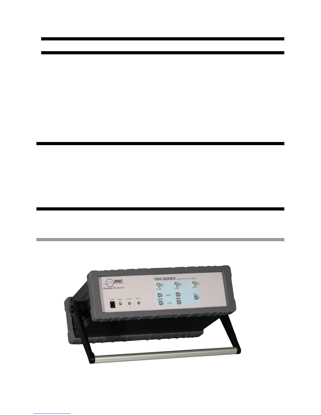
Figure 1: Model 7000 Series in 3U benchtop case

1 General Remarks

The instruments described in this manual are signal source analyzers that analyze electromagnetic
signals from 5 MHz up to 40 GHz with a power from -10 dBm up to +23 dBm. The exact range depends
on the chosen model and options. The instruments are able to perform different types of measurements,
such as absolute and additive phase noise, amplitude noise, transient analysis, spectrum monitoring, and
VCO characterization.

They can be used in a variety of applications such as research and development or manufacturing and
testing of electronic components.

Options, such as low noise internal references, amplitude measurements, measurements of pulsed
signals or a GPIB interface can be added.

1.1 Validity of this Manual

This manual is valid for the following instruments and their extended versions:

• Model 7070 (only serial numbers ending in a number greater than 0230)

• Model 7300 (only serial numbers ending in a number greater than 0230)

• Model 7340

1.2 Available Casing

The instruments are available in the following case.

1.2.1 3U Benchtop Case

5 7000 Series User Manual September 2017

1.3 Data Connections

The instruments may only be connected to a network or a computer by using a shielded LAN or USB
cable. Unless shorter lengths are prescribed, a maximum length of 3 m must not be exceeded for the LAN
and the USB connection.

1.4 Signal Connections

In general, all connections between the instrument and another device should be made as short as
possible and must be well shielded. It is recommended to use high-quality cables with low loss especially
for frequencies above 20 GHz.

1.5 Transportation

The instruments must only be transported with the packaging supplied by the manufacturer. The
instrument can be lifted up or transported in any orientation.

6 7000 Series User Manual September 2017

2 Safety Information

The following information is important to prevent personal injury, loss of life or damage to the instrument.
Please read them carefully. If the instrument is used in a manner not specified by this manual, the
protection provided by the instrument may be impaired.

2.1 Signal Symbol

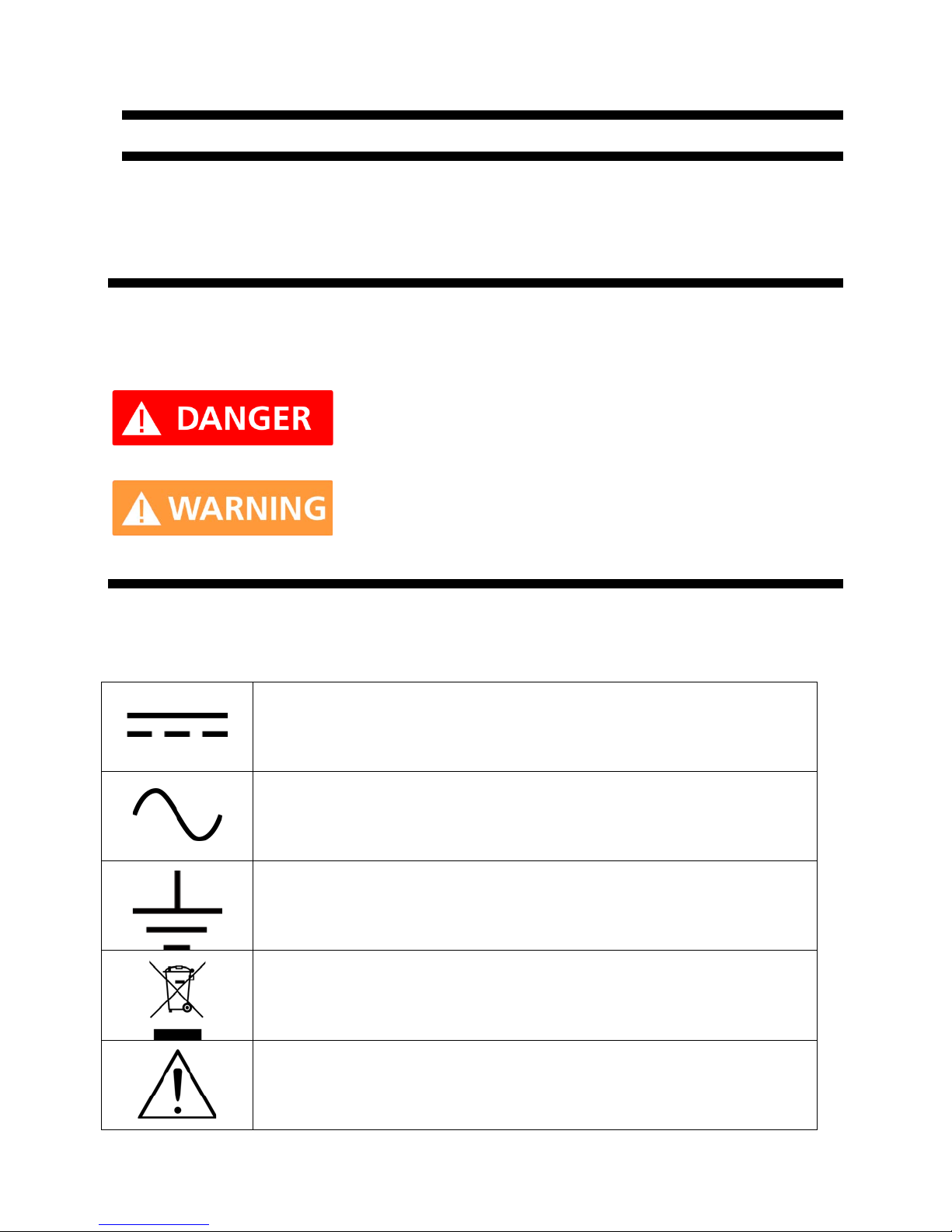
In this manual, the following symbols are used to warn the reader about risks and dangers.

DANGER denotes a hazard for personal health or life.

WARNING denotes a risk or danger that could damage the
instrument.

2.2 Labels on Products

The following labels are on the products. Familiarize yourself with the meaning of each of the labels before
using the product.

Direct Current (DC)

Alternating Current (AC)

Earth (Ground)

EU label for separate collection of electrical and electronic waste.

Caution, general danger zone. Attend the manual and/or a notice on the

7 7000 Series User Manual September 2017

device.

2.3 General Safety Considera ti ons

FCC notice
This equipment has been tested and found to comply with the limits for a Class A device, pursuant to Part

15 of the FCC Rules. These limits are designed to provide reasonable protection against harmful

interference when the equipment is operated in a commercial environment. This equipment generates,
uses, and can radiate radio frequency energy. If not installed and used in accor da nc e with the instr uc tio n
manual, harmful interference to radio communications may occur.

Operation of this equipment in a residential area may cause harmful interference in which case the user
will be required to correct the interference at his or her expense.

notice

The instrument meets the EMC directive and the Low Voltage Directive described below:
Safety: EN 61010-1.

EMC: EN 61000-6-4 (2006), EN 55022 (2008), EN 61000-6-2 (2005),
EN 61000-4-2 (2009), EN 61000-4-3 (2008), EN 61000-4-4 (2010),
EN 61000-4-5 (2006), EN 61000-4-6 (2009), EN 61000-4-11 (2004)

If products or their components are mechanically and/or thermally
processed in a manner that goes beyond their intended use, hazardous

substances (heavy-metal dust such as nickel) may be released. For this
reason, the product may only be disassembled or opened by specially trained personnel. Improper
disassembly may be hazardous to your health. National waste disposal regulations must be observed.

8 7000 Series User Manual September 2017

3 Technical Specifications

3.1 Dimensions

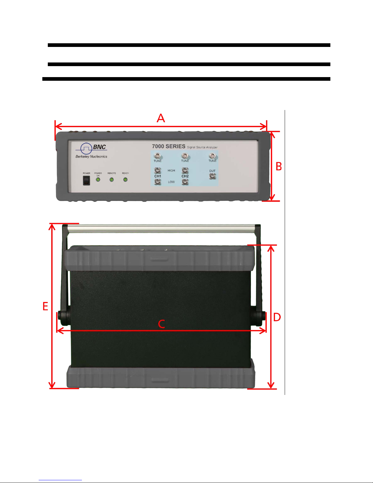
Dimensions of the 3U benchtop case:

A = 467 mm
B = 153 mm
C = 518 mm
D = 341 mm
E = 400 mm

Weight: 10 kg

Figure 2: Model 7000 Series benchtop case dimensions

9 7000 Series User Manual September 2017

3.2 Connectors

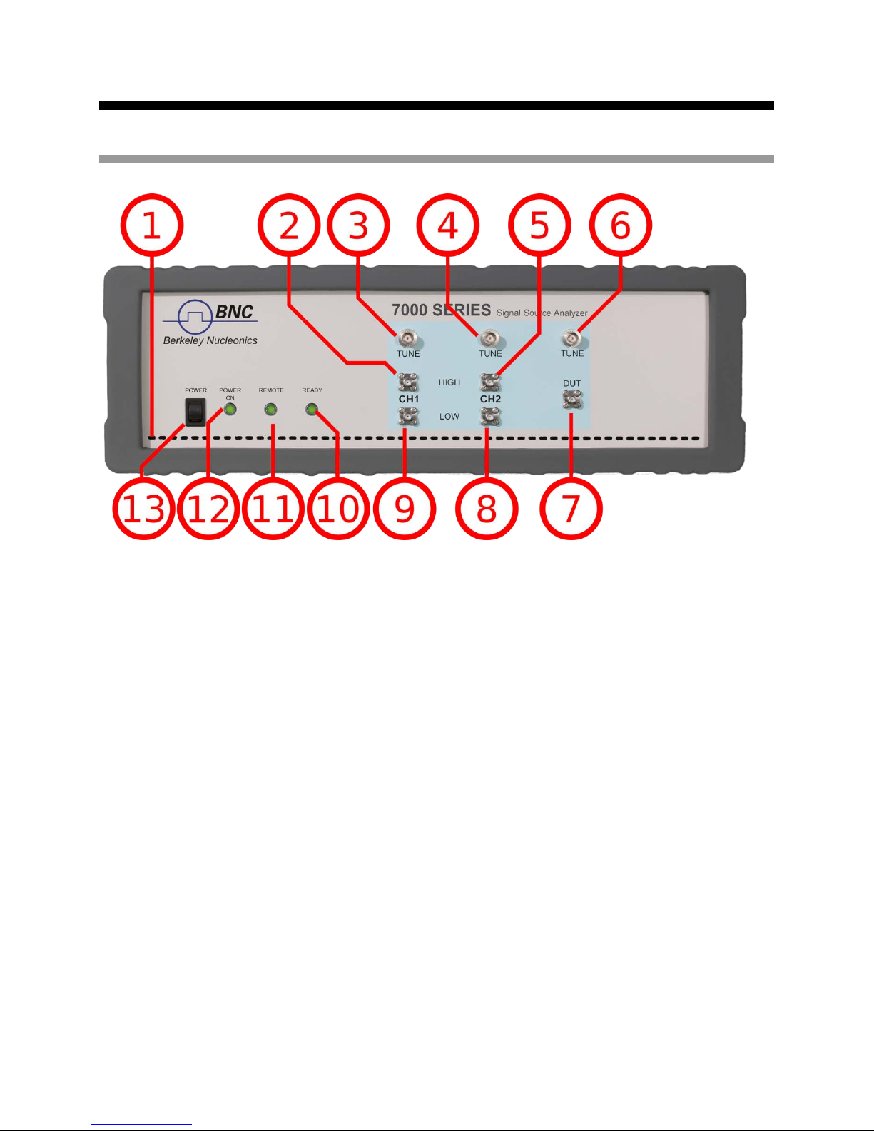
3.2.1 Front Panel

Figure 3: 7000 Series Front Panel View

1 Ventilation Slits Air inflow; leave open.

The front panel interfaces are grouped into three dark gray regions. Similar ports across different regions
are connected with a black line and are labeled once at the end of the line. The three regions are:

Reference region

2/5 REF1/2 IN HIGH These female SMA connectors are the high frequency RF inputs for

external reference channels 1 and 2. They are used for frequencies above 1.3 GHz.

3/4 REF1/2 TUNE port These female BNC connectors are the external reference tune

voltage outputs for channels 1 and 2.

DUT region

6 DUT TUNE port This female BNC connector is the tune voltage output for the Device

under Test (DUT), designed to supply a bias or control voltage for the DUT.

7 DUT RF IN port This female SMA or 2.92 mm connector is the DUT signal input. It is

AC-coupled and has an impedance of 50 ohms.

Reference region (cont’d)

8/9 REF1/2 IN LOW These female SMA connectors are the low frequency RF inputs for

external reference channels 1 and 2. They are used for frequencies below 1.3 GHz.

10 7000 Series User Manual September 2017

Instrument state region

10 Ready LED Indicates that the internal self-test on start-up was successful and that the

instrument is capable of performing measurements.

11 Remote LED Indicates whether the instrument is connected to a computer or not.
12 Power LED Indicates whether the instrument is on or off.
13 Power switch Disconnects the instrument from the DC power input completely.

Do not apply RF power levels above the maximum levels given in
the datasheet to the DUT/REF IN ports.

Do not apply a DC voltage or current to the DUT/REF TUNE outputs
or DUT/REF RF inputs. Applying a DC voltage or current may damage the instrument. In particular,
there is the risk of capacitors remaining charged. Connect DUT to the port after effectively
discharging the DUT's electricity.

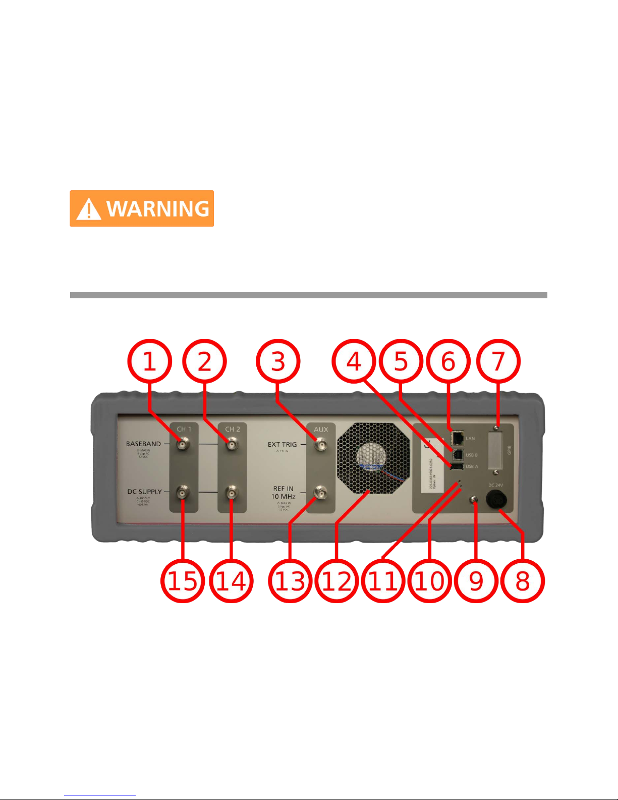
3.2.2 Rear Pan el

1 /2 BASEBAND IN port These female BNC connectors are the baseband signal inputs

used for the FFT analyzer measurement mode. They are AC coupled and have an
input impedance of 1 k ohms.

3 EXT TRIG port This female BNC connector is the external trigger input (TTL). The

maximum allowed DC level is 12 V, and the trigger threshold is 1 V +/- 0.1 V.

4 USB A connector Used for connecting USB devices such as memory sticks. This

function is currently not supported by the instrum ent .

11 7000 Series User Manual September 2017

Figure 4: 7000 Series Rear Panel View

5 USB B connector Used for connecting with a controller such as a PC or Laptop.

Communication is via USBTMC protocol.

6 LAN connector This 8 pin RJ-45 Host connector is used for connecting via Ethernet

with a controller, such as a PC or Laptop, with 10Base-T / 100Base-T Ethernet
(automatic data rate selection).

7 GPIB connector (optional) The connection of an external controller through General

Purpose Interface Bus (GPIB) connector enables configuration and control by an
automatic test equipment (ATE) system. This GPIB connector is used solely for
controlling the 7000 Series from an external controller, and cannot be used as a
control connection for other devices.

8 DC IN power receptacle The power receptacle accepts the 4-pin plug from the external

24 V DC power adapter that is supplied with the instrument.

9 Ground Screw
12 FAN Holes Air outflow; leave open.
13 REF IN 10 MHz This female BNC connector is the 10 MHz reference clock input. The

maximum allowed DC level is 12 V, and the maximum allowed AC level is 2 Vpp.

14/15 DC SUPPLY OUT ports These female BNC connectors are the programmable low-

noise DC supply voltage outputs.

The serial number plate shows the serial number and the installed options of the instrument.

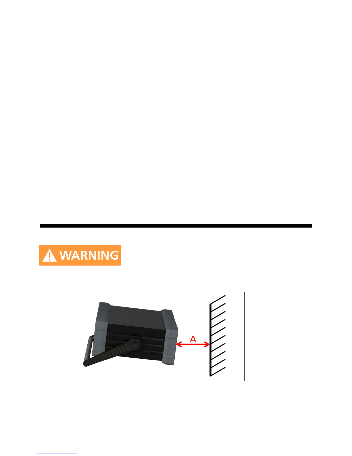
3.3 Minimum Distances

For adequate cooling, the minimum di stances between the
instrument and another object, such as walls, rack cabinet walls or
other equipment must be respected.

The minimum distances are:

Minimum distance:
A: 150 mm

12 7000 Series User Manual September 2017

Figure 5: 7000 Series benchtop case cooling

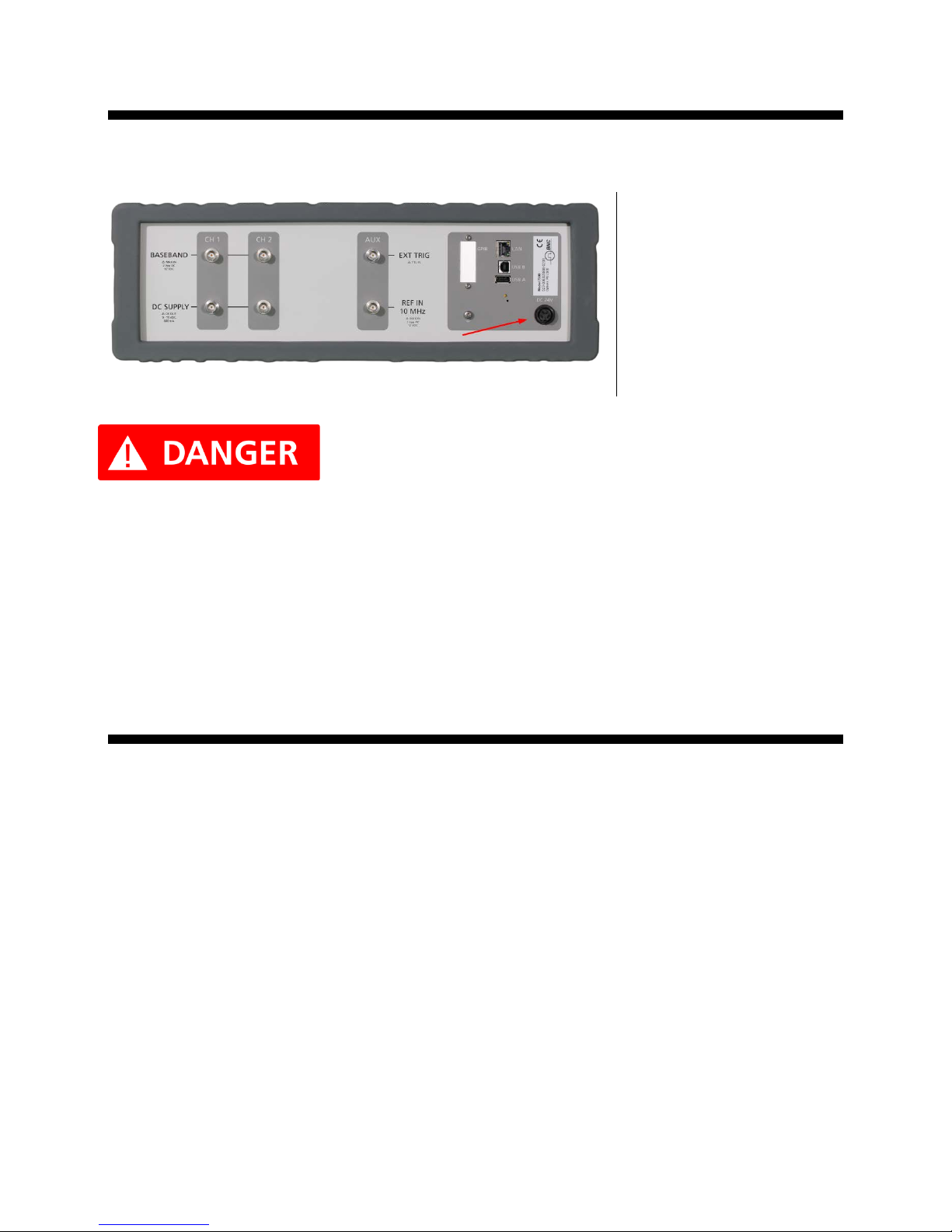
Figure 6: 7000 Series power connector

3.4 Energizing and de-Energizing

To energize the instrument, apply the following voltage to the following connector.

Position of the power
connector shown on the
left.

Voltage: 24 V DC
Max. current: 2.7 A

Use the supplied power adapter from Berkeley Nucleonics to supply
the Instrument. Apply only a voltage with the values specified
below.

The supplied power adapter has the following specifications:

Input: 100-240 V~, 50-60 Hz, 1. 4 A
Output: 24 V DC, 2.7 A
Efficiency Level: VI

To De-energize the instrument, pull out the power cable.

3.5 Operation Conditions

The instrument is designed for use in dry and clean environments. The instrument can also be used in the
field as long as the operating conditions are met. Operation in an environment with high dust content, high
humidity, danger of explosion or chemical vapors is prohibited.

Operating temperature range: 0° C to +40° C
Storage and transportation temperature range: -40° C to +70° C
Operating and storage altitude: 4600 m

In case of condensation, 2 hours are to be allowed for drying prior to operation. Operation is only allowed
from a 3-terminal mains connector with a safety ground connection and a mains plug used in your specific
country. For sufficient ventilation, ensure open ventilation holes.

13 7000 Series User Manual September 2017

3.6 Environmental Information

Electrical and electronic equipment waste must not be disposed of with unsort ed municipal waste, but
must be collected separately. Contact Berkeley Nucleonics Customer Support for environmentally
responsible disposal of the product .

Specially marked equipment has a battery or accumulator that must not be disposed of with unsorted
municipal waste, but must be collected separately. It may only be disposed of at a suitable collection point
or via Berkeley Nucleon ic s Customer Support.

14 7000 Series User Manual September 2017

4 Introduction

This instruction manual is valid for the Berkeley Nucleonics 7000 Series . Chapters 5 and 6 give you
guidance for a quick and easy setup of your new instrument. Chapter 6 describes the remote operation via
Berkeley Nucleonics graphical user interface (GUI). Chapter 7 describes the remote operation via the
SCPI API. Section 8.1 explains the steps to calibrate the system.

4.1 General Features and Functions (Model Overview)

Berkeley Nucleonics Signal Source Analyzer model overview

Model Range Options available

MODEL 7070

MODEL 7300

MODEL 7340

General features include

• Absolute and additive phase noise measurements

• Transient Analysis

• Spectrum Monitoring

• VCO Characterization

• Dual channel supply voltage ports

• Standard internal references

• Long-term support: Software upgrades (firmware, API, GUI) are available to download from

www.BerkeleyNucleonics.com

continue to use both of these services free of charge for the lifetime of the product.

• Universal LAN VXI-11 and USB 2.0 device interface

5 MHz – 7 GHz LN, AM, PULSE, GPIB

5 MHz – 26.5 GHz LN, AM, PULSE, GPIB

5 MHz – 40 GHz LN, AM, PULSE, GPIB

. You can also call our technical specialists for support. You can

• 24 months calibration cycle

15 7000 Series User Manual September 2017

4.2 Options

LN: Low noise internal reference
AM: Amplitude noise measurements
PULSE: Measurement and analysis of pulsed RF signals. Supports the following measurement modes:

• Absolute phase noise

• Additive phase noise

GPIB: GPIB interface added
WE3 / WE5: Warranty extension to 3 or 5 years (standard warranty covers 2 years)

16 7000 Series User Manual September 2017

5 Getting Started

5.1 System Requirements

The graphical user interface has minimum system requirements in order to run on one of the supported
operating systems. Since the graphical user interface is Java based, it is also possible to run it on any
operating system that can provide a Java Runtime Environment. Please contact technical support if you
need to run it on a non-Windows computer.

Operating system Windows™ XP SP2, Vista, 7, 8, 10
Hardware requirements min. 4 GB RAM, min. screen resolution of 1280x1024
Remote 10/100/1000M Ethernet or USB 2.0 Port

5.2 Unpacking the Instrument

Remove the instrument materials from the shipping containers. Save the containers for future use.
The standard product package includes :

• Signal Source Analyzer

• Ethernet Cable

• Universal DC power adapter

• Software & Manual CD

• Test Certificate

5.3 Initial Inspection

Inspect the shipping container for damage. If the container is damaged, retain it until contents of the
shipment have been verified against the packing list and instruments have been inspected for mechanical
and electrical operation.

5.4 Starting the Instrument

This section describes installation instructions and verification tests.

5.4.1 Applying Power

Place the instrument on the intended workbench and connect the power adapter to the receptacle on the
rear of the instrument. Make sure to use the power adapter supplied with the instrument.

17 7000 Series User Manual September 2017

Using other supplies may lead to malfunction and damage of the
Instrument.

Use the power switch on the front panel to turn on the 7000 Series. The green LED marked POWER on
the front panel will indicate that the power supply is connected and the instrument is starting. During the
initialization process, the green LED marked READY will start to flash briefly. This indicates that the
machine performs a self-test. Once the READY LED is on steadily, the instrument is ready for operation.

Note, the instrument booting process may take up to 60 seconds (depending on configuration) to
complete.

5.4.2 Connecting to LAN via DHCP Router

Connect the instrument to your local area network (LAN) using the Ethernet cable. By default the
instrument is configured to accept its dynamic IP address from the DHCP server of your network. If it is
configured properly, your net work router will as sign a dynamic IP address to the instrument.

5.4.3 Direct Connectivity to Host via Ethernet Cable (no Router)

You can connect the instrument to your computer with the Ethernet cable without using a local area
network with DHCP server. To work properly, the network controller (NIC) of your computer must be set
to a fixed IP beginning with 169.254.xxx.xxx (excluding 169.254.1.0 and 169.254.25 4.25 5) and network
mask 255.255.0.0 to match the fall-back IP that the 7000 Series will assign itself after network timeout.
The 7000 Series will automatically choose an IP address according to ZEROCONF standard. Therefore,
the exact fall-back address can’t be predicted.

Connection from a NIC that is configured to use DHCP is also possible. After a pre-set timeout, the NIC
will assume that no DHCP is available and self-assign a fall-back IP that will fall into the range

169.254.xxx.xxx.
Alternatively, you may assign the instrument a fixed IP. Please refer to a later section of this manual to

learn how to do this.

5.4.4 Connecting through USB

Connect the (powered on) instrument USB B connector on the rear panel to the computer using a USB
cable. If properly connected, the computer host should automatically recognize your instrument as a
USBTMC device.

Note if you want to work with the graphical user interface, it must be installed with USB support selected.
The GUI will detect all connected instrum ents automatically. Open the GUI and follow the instructions
given in Chapter 6.

Alternatively, a VISA runtime environment (NI or Agilent or comparable) must be installed.
Use VISA Write to send the *IDN? query and use VISA Read to get the response. The USBTMC protocol

supports service request, triggers and other GPIB specific operations.

5.4.5 Connecting through GPIB

Connect the instrument to the GPIB controller using the rear panel GPIB connector (option GPIB is
required). Once connected properly, use VISA Write to send the *IDN? query and use VISA Read to get
the response. The protocol supports service request, triggers and other GPIB specific operations.

18 7000 Series User Manual September 2017

5.4.6 Using the SCPI Application Programming Interface (API)

Refer to the 7000 Series Programmer's Manual to learn more about applying the API and find
programming examples.

5.4.7 Installing the 7000 Series Graphical User Interface (7000 Series GUI)

Berkeley Nucleonics's graphical user interface (7000 Series GUI) provides an intuitive control of the 7000
Series . The Java based application runs under any operating system, including Windows XP, Vista, 7, 8
and 10 with standard requirements. Only the Java runtime environment must be installed on the computer.

To install the GUI on the computer, insert the 7000 Series Software and Manual CD into the CD/DVD
drive, or download the latest GUI setup file from the Berk ele y Nucleon ic s website. If the setup doesn't start
automatically, double click on the setup.exe to run the installer.

The self-extracting setup provides easy installation, and un-installation, of the software. The setup
program guides you in a few steps through the installation process. In case the Java Runtime
Environment is not installed on the current computer, the setup pr oc e dure wi ll ass is t you with the
installation of the required version. An active internet connection is required for this operation.

5.4.8 Troubleshooting the LAN Interconnection
Software does not install properly

• Make sure your installation CD is not damaged.

• Verify that the Java Runtime Environment is installed and up to date.

Software cannot detect any instrument

• Make sure that you have connected both the computer and the instrument to a common network.
If they are not in the same subnet, the search won't show the instrument. The devices can still be
connected by manually setting the IP address in the connection dialog.

• If a direct connection is used, you may be required to reset your computer Ethernet controller
(depending on the configuration). In such a case, note that detection of the instrument can take a
considerable amount of time if your computer is configured to work with an external DHCP server.
In some cases the detection may even fail completely. Configure your computer network controller
to an appropriate fixed IP address instead.

• Make sure that your software firewall enables the GUI to setup a TCP/IP connection via the LAN.
Under Windows 10 you can do that like this:
Open the Control Panel in your Start menu. Go to System and Security and then to Windows
Firewall. Click on Allow an app or feature through Windows Firewall and then on Change Settings.
You can now select the check box for the application on your computer. Click the private and
public check box to narrow down whether you want just networks that are secure to allow this
communication, or also public and non-secure networks to do so. Now your Windows™ Firewall
will not block requests from the GUI.

5.4.9 Shutting Down the 7000 Series

Use the power switch on the front panel to turn the instrument off.

19 7000 Series User Manual September 2017

5.4.10 Perform Firmware Upgrade

If the GUI has internet access, it will check for newer firmware versions upon connection to the instrument.
If there is a newer firmware available, the GUI will notify you. If you confirm the upgrade, the firmware will
automatically be downloaded and installed on the instrument.

If the GUI has no internet access, a firmware upgrade of the instrument can also be done manually via the
GUI. Ensure proper connection and that the correct firmware binary is available. Then navigate to Device

-> Update Firmware and select the appropriate binary (tar file) that you have received from Berkeley
Nucleonics, or downloaded from the Berkeley Nucleonics website. The update will take a few minutes,
and after completion the instrument will reboot. Reconnect to the instrument.

Do not switch off or disconnect the instrument during the firmware
upgrade procedure. Interrupting the procedure can result in a
damaged or non-responsive instrument.

5.4.11 Serial Number

Each instrument is manufactured with a unique serial number shown on the sticker on the rear panel. This
serial number is also internally stored, and determines the instrument configuration and guides the
software accordingly.

20 7000 Series User Manual September 2017

6 Using the Graphical User Inter f a c e (GUI )

The graphical user interface (7000 Series GUI) provides an intuitive control of the instrument and the
measurement processes. It runs under any operating system supporting a Java Runtime Environment
(JRE). Ensure that the software is installed and the computer’s firewall is configured properly.

6.1 Starting the 7000 Series GUI

Double-click the 7000 Series shortcut that will appear on the desktop after the software has been
successfully installed. Ensu r e that the 7000 Seri es is turned on and connected to the computer using
either Ethernet or USB connectivity.

After start-up, the software will automatically detect existing 7000 Series instruments (LAN and USB) and
will establish connection to the previously connected device, if still available. Otherwise a window will
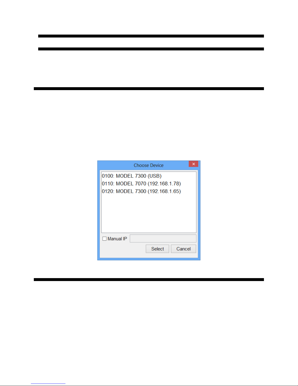
appear with all detected 7000 Series devices listed. Connection to a device can be established by
selecting the device identifier in the list and then clicking on the “select” button. When this dialog is
displayed, the GUI continuously searches and refreshes the list of available devices.

6.2 Organization of the GUI

The measurement window is organized as shown in Figure 8. The GUI is divided into three sections: a
setup section on the top left, a plot configuration section on the top right, and the actual measurement
window on the bottom.

21 7000 Series User Manual September 2017

Figure 7: Device selection dialog

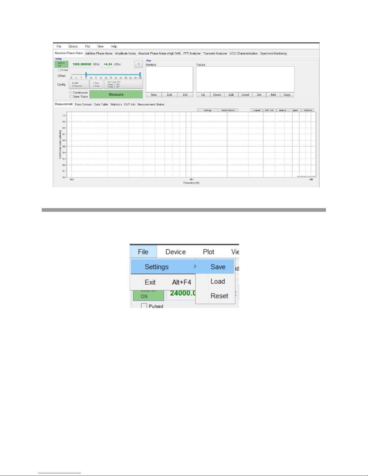
Figure 8: GUI after startup.

6.2.1 Menu Bar

The drop-down menus File, Device, Plot, View, and Help are located in the upper left of the GUI window
and are described below:

Figure 9: GUI File menu

6.2.1.1 File Menu
File  Setting -> (Save, Load, Reset) allows storage and restoring of user defined parameters and

measurement settings. When the GUI exits, the current configuration is automatically saved and restored
at the next restart.

File  Exit will terminate the GUI software.

6.2.1.2 Device Menu
Device  Connect automatically detects available 7000 Series devices connected via Ethernet or USB. If

a connection is already established, this option disconnects and opens the dialog as shown in Figure 7.
Device  Disconnect will terminate an existing connection to an instrument.

22 7000 Series User Manual September 2017

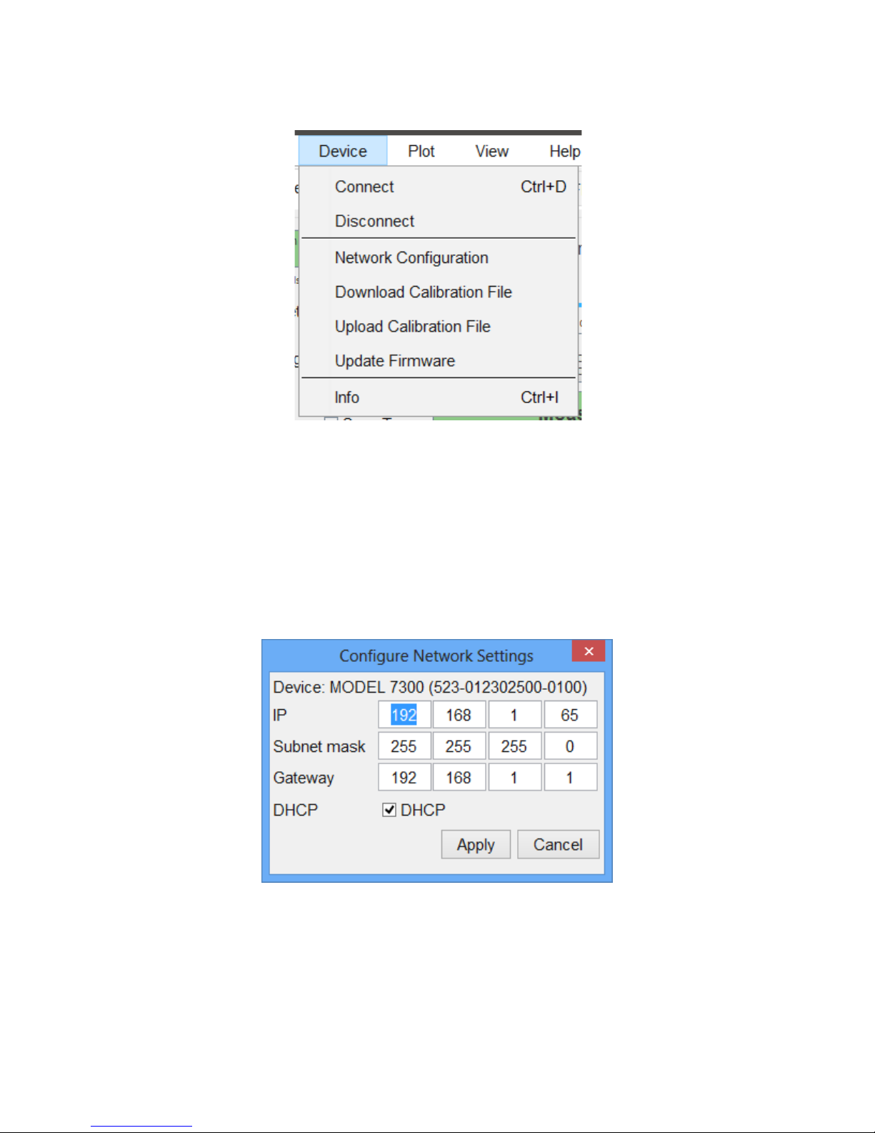
Figure 10: GUI Device menu

Device  Network Configuration allows reconfiguration of instrument network settings, such as IP,

subnet mask, or gateway. If your network does not have a DHCP (dynamic host configuration protocol)
server, or if a static IP address is preferred, you can set an IP address, network mask and default route.
The address and mask settings are required. The default route is not strictly necessary but enables
network communication between the instrument and devices on a subnet other than that to which it is
immediately attached. The network features can be used on the local area network even if no default route
(specified as 0.0.0.0) is configured.

Any change will be effective after a subsequent hardware reboot of the device.

Figure 11: GUI Device Network Configuration dialog

Device  Update Firmware performs a firmware update. A dialog window will ask for firmware file (.tar).

After selecting a correct firmware file, the update will proceed for approximately 5 minutes. The GUI will
disconnect from the instrument during the update process.

23 7000 Series User Manual September 2017

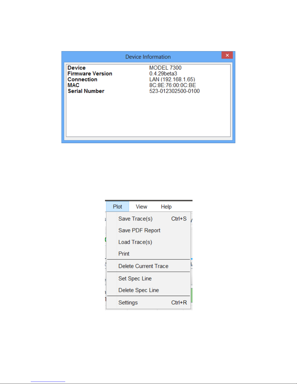
Device  Info provides product details of the instrument such as firmware version, instrument serial and
options installed as shown below.

Figure 12: GUI Device Information

6.2.1.3 Plot Menu
Plot  Save, Load, Print allows storing, loading and printing of the plot windo w . Plots can be saved as

PNG images or in 7 000 Ser ies internal file format (extension .7000 Series ). They later can be loaded into
the GUI. Data traces can also be exported when saved as MATLAB™, MS EXCEL™, or CSV files
(extension .csv).

Plot  Save PDF Report auto-generates a PDF report including measurement trace, jitter data, Allan
Deviation plot, phase noise, spurious and marker data of the currently selected measurement.

Plot  Delete Current Trace deletes the active measurement trace.

24 7000 Series User Manual September 2017

Figure 13: GUI Plot men u

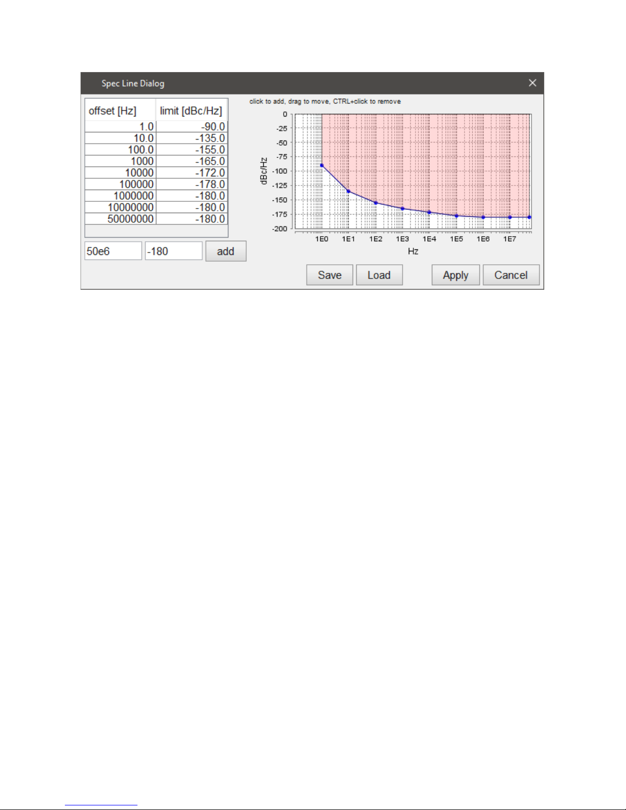
Figure 14: GUI Plot Spec Line dialog

Plot  Set Spec Line opens a window dialog that allows defining and drawing a s pec line into your

measurement window. The data can be input manually in table format on the left, or by clicking into the
window on the right. Spec lines can be saved into, and loaded from, an external file.

Plot  Delete Spec Line deletes the currently loaded spec line.
Plot  Settings opens the plot configuration dialog as shown below. The dialog allows customization of

the plot window. Window title, font size of the text displayed on the plot, legend labels and plot background
color can be configured in this dialog. In the lower section of the dialog, the axes can be scaled and
renamed.

25 7000 Series User Manual September 2017

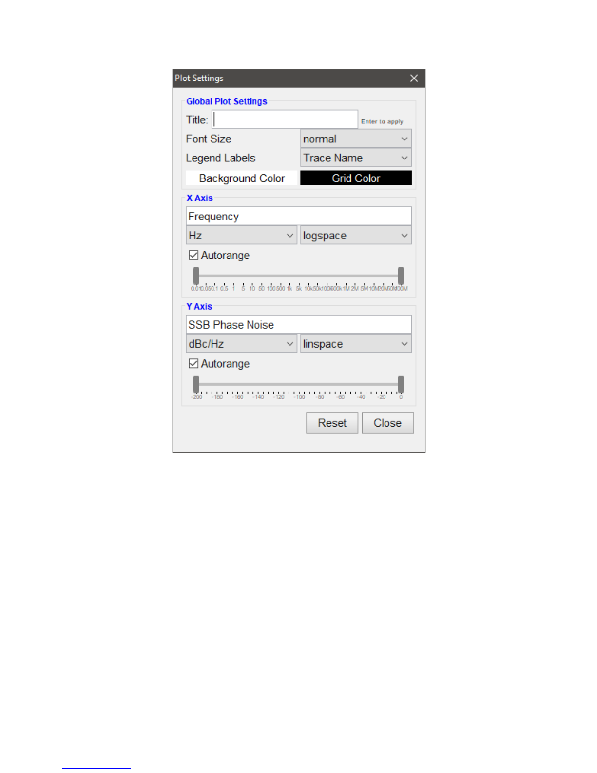
Figure 15: GUI Plot Settings dialog

6.2.1.4 View Menu
View  Toggle Fullscreen allows toggling from and to full screen mode.

6.2.1.5 Help Menu
Help  Switch to Service Mode is used by Berkeley Nucleonics engineers only, and is used to calibrate

the device. Currently, customers cannot activate this option.
Help  Activate Logging logs status and error information from the GUI into a binary file. This file can

then be sent as part of an error report to the Berkeley Nucleo nics s upp ort em ail. This should not be
activated during normal use as the logging slows down the application which can affect the user
experience.

26 7000 Series User Manual September 2017

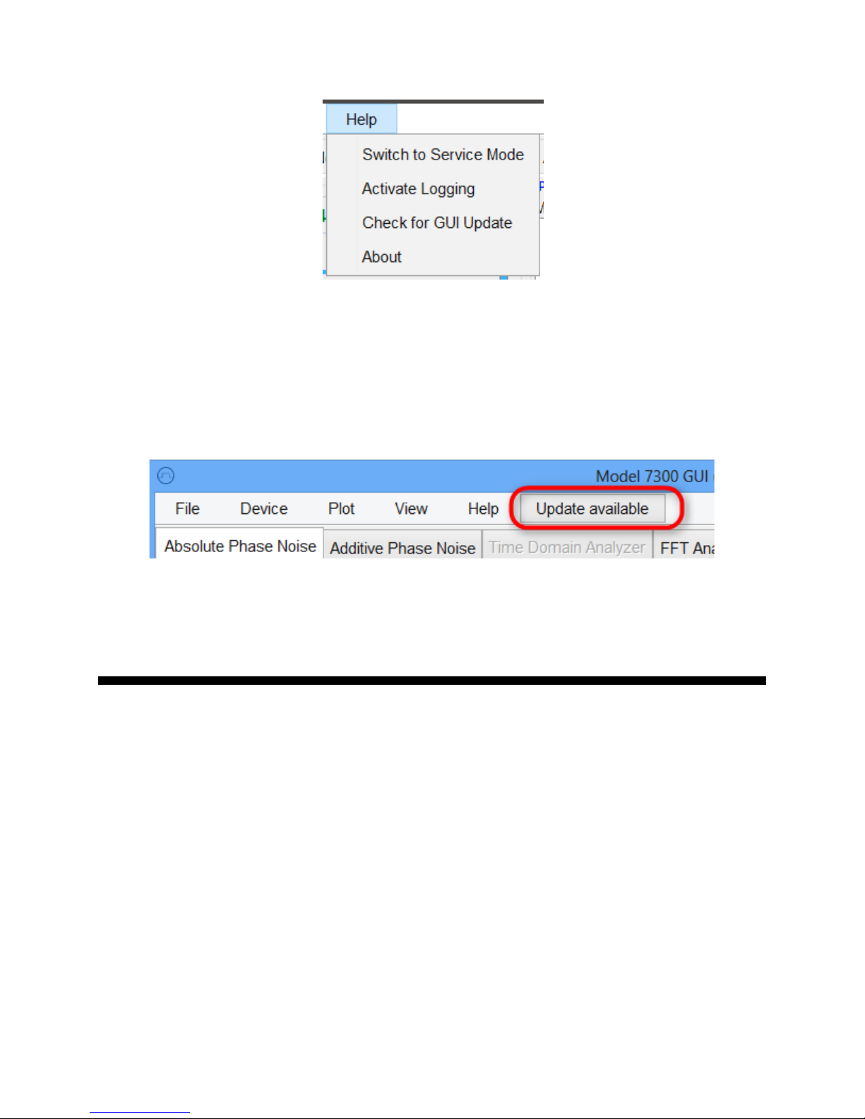
Figure 16: GUI Help menu

Help  Check for GUI Update can be used to verify if a newer version of the GUI is available for

download from the Berkeley Nucleonics website. If a new version is available, it can be downloaded and
installed directly.

Help  About displays the GUI version information.

6.2.1.6 Update Button

Figure 17: GUI Update message

If the computer is connected to the internet, it will check for a new version on startup. If there is a new
version available, the GUI will provide a notification by displaying an update button on the right side of the
menu. Clicking it will start the update procedure.

6.3 Measurement Tabs

The following tabs (each corresponding to a particular measurement mode), are available:

• Absolute Phase Noise

• Additive Phase Noise

• Amplitude Noise

• Absolute Phase Noise (High Drift)

• FFT Analyzer

• Transient Analyzer

• VCO Characterization

• Spectrum Monitoring

Clicking on a tab will lead to the corresponding measurement setup. The following sections describe each
measurement mode and how to configure the 7000 Series to successfully perform a measurement.

27 7000 Series User Manual September 2017

6.3.1 General Tab Organization

In general, each measurement tab is organized in two sections, a setup and a plot section. The setup
section in the upper left corner is used to configure a particular measurement. The plot section is used to
display and enable post-processing of measured data.

6.4 Absolute Phase Noise Measurement Tab

Use this tab to measure absolute phase noise of a continuous waveform (CW) or a pulse modulated
signal.

The device under test’s (DUT's) signal frequency and power is detected and the phase noise of the signal
in the specified offset frequency range is analyzed. The measurement principle is based on the phase
discriminator method in combination with a two channel cross-correlation system. Two internal or external
low noise reference sources are phase locked to the DUT signal. The frequency of the DUT is detected
and a well characterized phase locked loop is closed. Each receiver channel now converts phase
fluctuations between DUT and the reference source into low frequency voltage signal by means of a
calibrated phase detector. Inside the PLL bandwidth, the phase differences are suppressed and must be
recovered. The two independent measurement channels are fed into FFT analyzers and a cross­correlation engine to suppress reference and receiver channel noise, and to extract DUT phase noise.

6.4.1 Measurement Setup

The following section describes the basic setup procedure to perform a measurement within the Absolute
Phase Noise measurement tab. With just a few configuration steps, the phase noise measurement can be
performed.

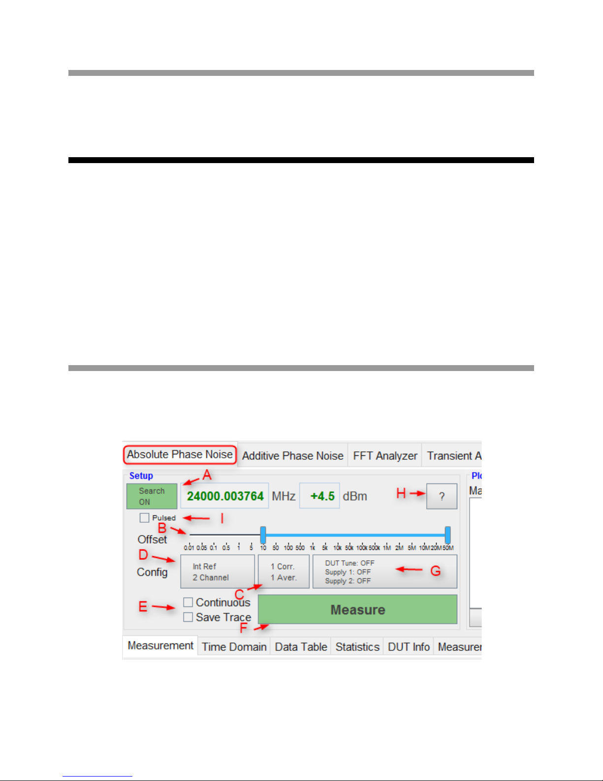
Figure 18: Setup section of Absolute Phase Noise tab

28 7000 Series User Manual September 2017

A) Enable internal fr equency counter and power meter (see Figure 18): If the search button is

enabled, the counter and power meter are running, and constantly updating the detected DUT's
frequency and power. Disabling allows manual entry of the DUT frequency, and internal counters
and power detector are in the off state. By default, the auto-detection is on, and once a valid
signal is detected, the measure button turns green and is enabled.

B) Set frequency offset range using the slider. The frequency offset can be set freely from 0.01

Hz up to 50 MHz depending upon your particular Series 7000 Model..

C) Select the number of correlations/averages: The number of correlations and averages can be

set by clicking on this button, which will open up a dialog that allows the user to set the
parameters to predefined values via drop down menu. Exact values can also be manually
entered.

D) Use the reference button to select between internal and external reference sources. By

default, the internal sources are used and no additional configuration is needed. See the section
“Using external references” for more information about how to use external references.

29 7000 Series User Manual September 2017

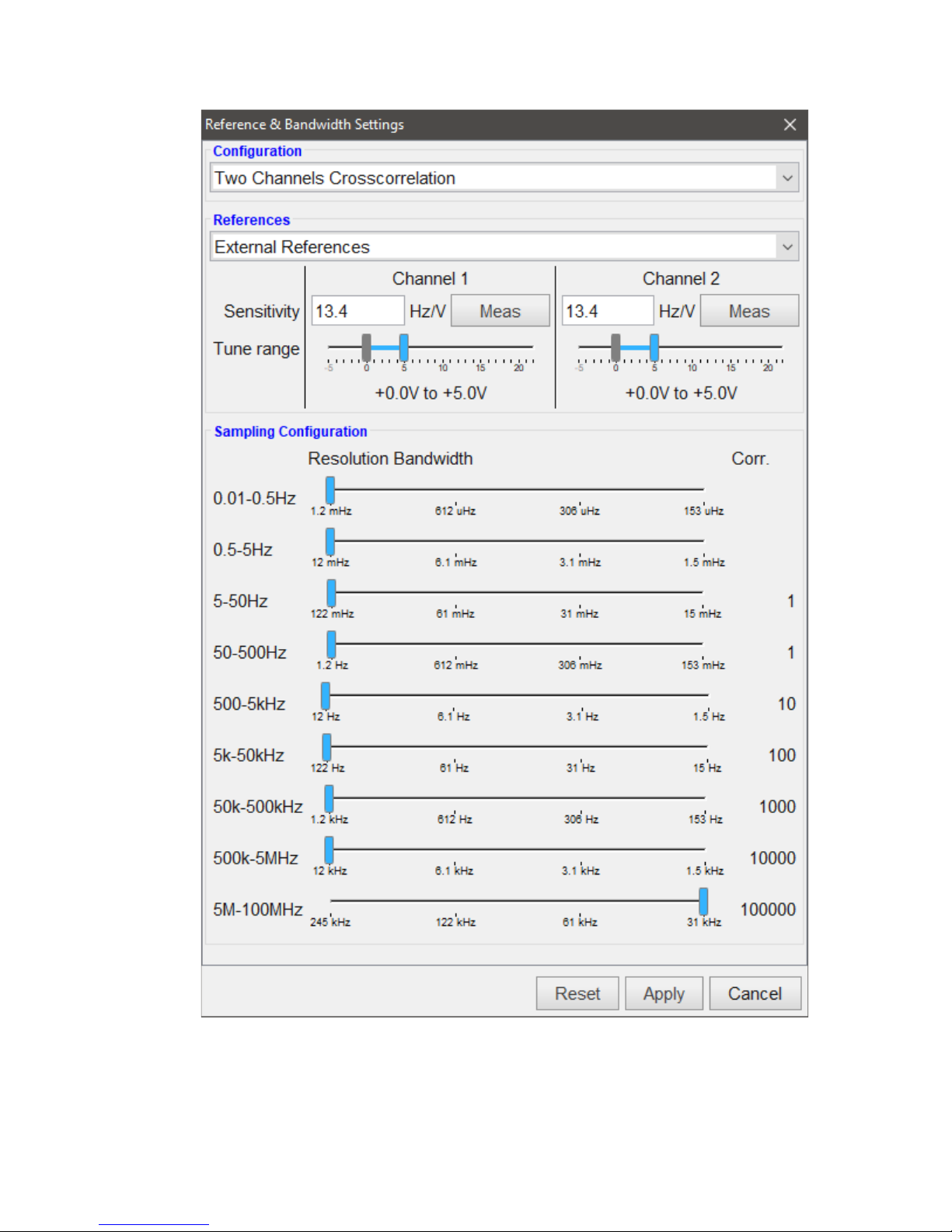
Figure 19: Advanced Configuration menu allows choosing reference source

The advanced measurement configuration dialog also gives the option to change the internal
reference mode between standard, high sensitivity and low noise (optional).

30 7000 Series User Manual September 2017

Standard References: This is the default option that is available in all 7000 Series models. It
uses references with reasonably high tuning sensitivity and very good phase noise characteristics.
It is suited for almost all applications.

High Sensitivity References: These references have a very high tuning range at the cost of
decreased phase noise performance for offset frequencies below 100 Hz. They are used for
unstable DUT's with high frequency drift that cannot be locked with the standard references.

Low Noise References: References with very low phase noise. This comes at the cost of a
decreased tuning range, and is only suitable for DUTs with stable frequency behavior. Unlike the
other modes, the low noise references require a five minute warm-up time. This is indicated by an
orange measure button upon selection. The Measure button will turn green again once the
references are ready.

In the sampling configuration section of the dialog, the resolution bandwidth (RBW) of specific
frequency offset ranges can be changed. The resulting number of correlations for the change,
combined with the current measurement setup (offset range, number of correlations) will be
displayed on the right side of each slider.

E) Configure Continuous & Save Trace Options: With “Continuous” enabled, the measurement is

restarted automatically after completion.
With “Save Trace” enabled, the trace of a completed measurement is automatically imported and

stored in the Trace List.

F) Click Measure Button: Once the Measure button becomes green, a new measurement can be

initiated. Click on the button to start the measurement and click again to stop the measurement
before completion.

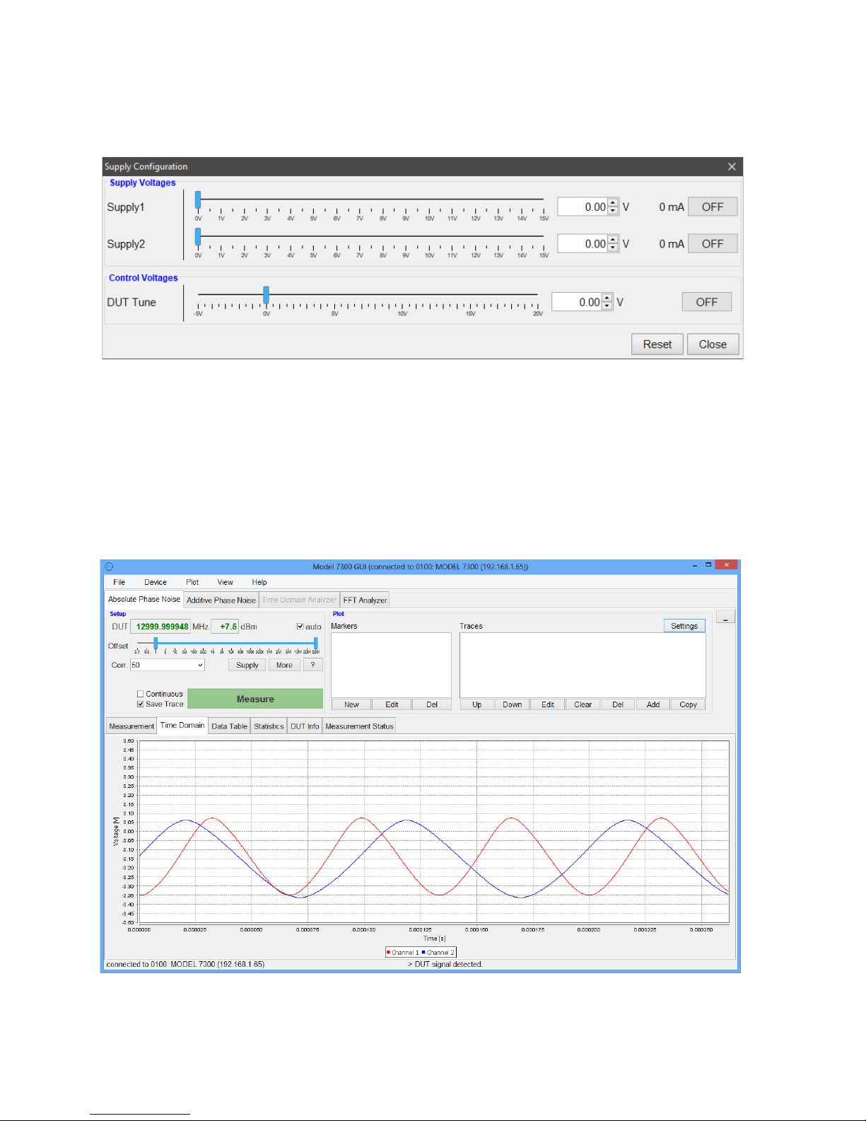
G) C o n figure Supply: If available with the currently connected device, this button will open the

supply dialog in which the output voltage on the DC SUPPLY ports on the back panel and the
DUT TUNE port on the front panel can be configured (as shown in Figure 20). The supplies can
be separately set, enabled/disabled, and the current is measured continuously. The DUT tune port
can be configured to output a constant voltage. This can be used, for example, as bias voltage for
the DUT.

H) Connection Diagram: Clicking on the button with the question mark will open a connection

diagram that represents the currently selected measurement setup. For a basic phase noise
measurement, this diagram is very simple. But it can be helpful for more difficult measurement
setups, like a two-channel, external references measurement or an additive phase noise
measurement.

31 7000 Series User Manual September 2017

I) Pulsed Measurements: In order to perform a phase noise measurement of a pulsed signal, the

pulsed option has to be activated using this checkbox.

Figure 20: Supply Configuration dialog

After clicking on the Measure button, the phase noise measurement is initialized. A couple of calibration
steps are automatically performed and phase noise data is acquired from the 7000 Series . In the
Measurement tab of the plot window, the red trace shows the intermediate result as shown in Figure 22.

Once the measurement is completed, the GUI returns to idle state. During the idle state, the “beat” signal
of the two measurement channels can be observed in the Time Domain tab of the measurement window,
as shown in Figure 21.

Figure 21: Beat frequency as shown in the Time Domain tab within the plot window

32 7000 Series User Manual September 2017

At the start of a measurement, the 7000 Series will adjust the input attenuation/gain to avoid power
compression and maximize dynamic range, calibrate the phase detector, and phase lock the internal
references. The “Measurement Status” tab will indicate measurement progress and provide status and
error messages.

The loop bandwidth is adaptively set to ensure stable and reproducible measurements with maximum
dynamic range. The gain of the IF amplifiers is adjusted to measure at highest sensitivity without driving
the amplifier stages into compression.

Note, the measurement time largely depends on the minimum offset frequency and the total number of
correlations.

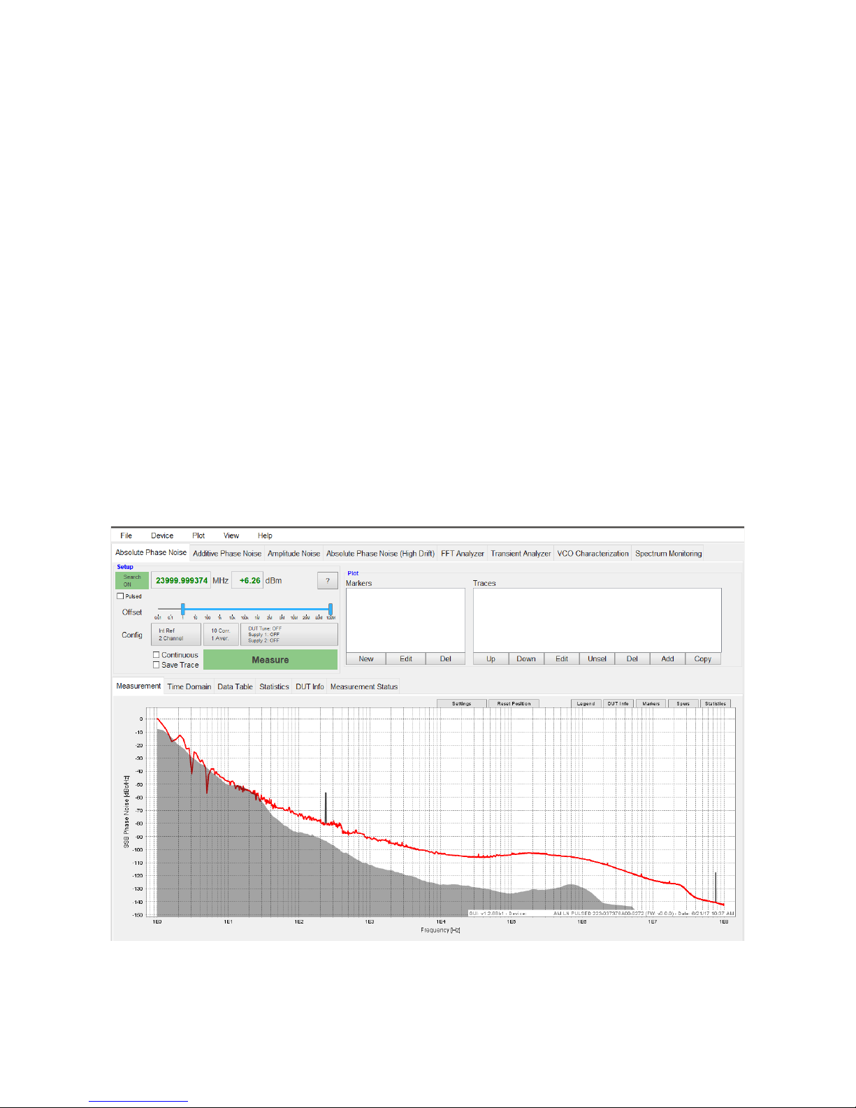
Figure 22 shows a screenshot of the GUI after a completed measurement. The measurement trace is
shown in red. Spurs are displayed in black. Below the measurement trace, a gray polygon (shade trace) is
visible. This polygon indicates the relative measurement floor for the current measurement. With a larger
number of correlations, the noise floor will decrease. If the measurement trace at a given offset is above
the noise floor, the measured trace has reached a steady-state value at that offset. At this point,
increasing the number of correlations will only “smooth” the curve and remove trace noise, but will not
further improve the phase noise value.

33 7000 Series User Manual September 2017

Figure 22: Phase Noise measurement completed

6.4.2 Pulse d Si gnal Phase Noise (with Option PULSE only)

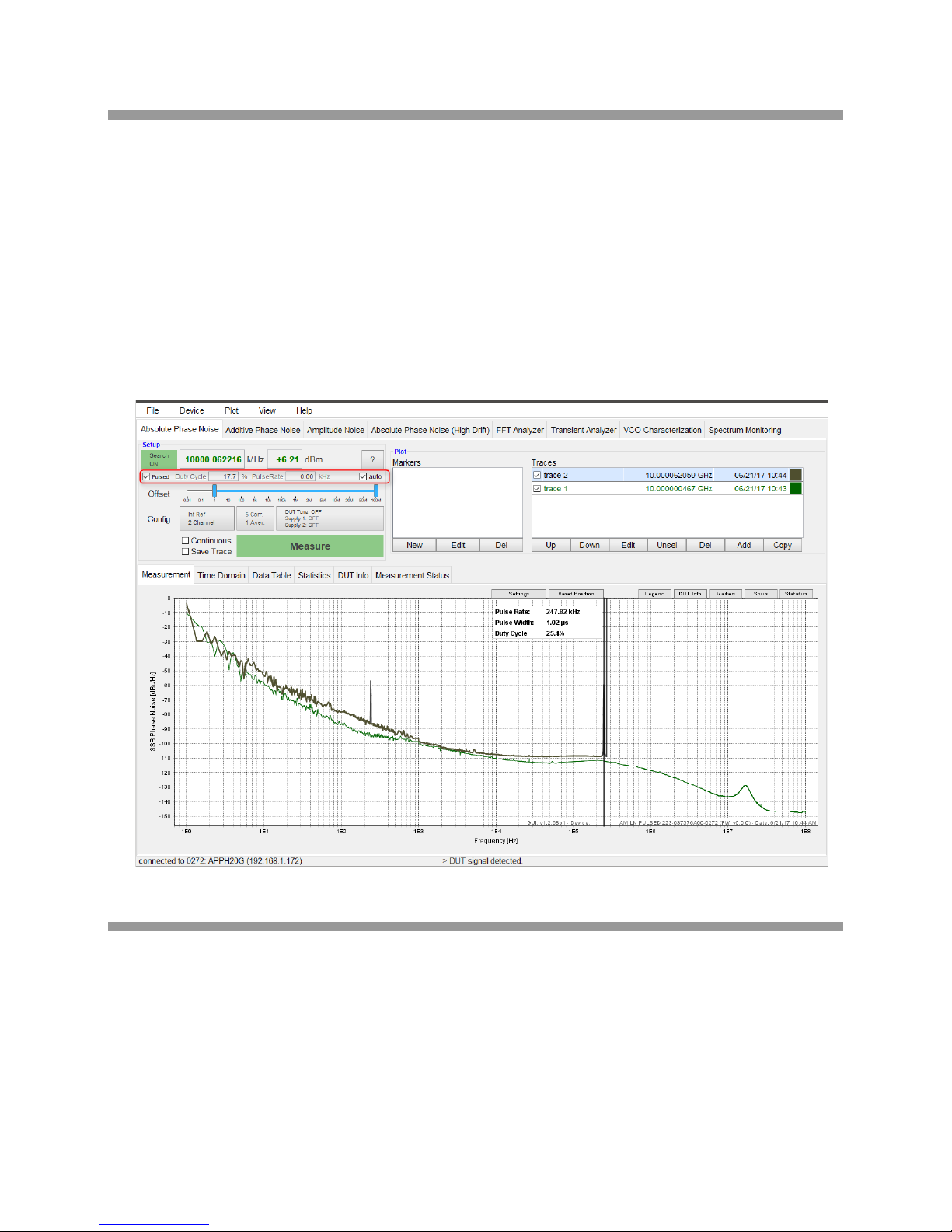
The 7000 Series can be configured for pulsed signal measurements by activating the “Pulsed Mode”
check-box above the offset range slider (marked red in Figure 23). By pressing the green Measure button,
the 7000 Series will automatically detect all the necessary parameters such as pulse width, pulse rate
and duty cycle and adjust the measurement process accordingly. If the input signal is not detected as
pulse modulated, a standard phase noise measurement will be performed.

The resulting trace will only be shown for offset frequencies up to the detected pulse rate. The pulse rate,
pulse width and duty cycle are shown as a visual overlay over the trace selected. Figure 23 shows the
completed measurement of a pulse modulated signal.

Figure 23: Absolute Phase Noise measurement of a pulsed signal

6.4.3 Using External References

Configuring external references requires some additional parameter settings.

A) Number of Channels: Select one channel or two channel (cross correlation) measurement.

B) Tuning slope and range: Enter tuning slope (Hz/V) for each measurement channel used. Also

enter the tuning voltage range for each reference. Using the Measure button, the tuning slope can
also be measured automatically, once the tuning range has been set.

34 7000 Series User Manual September 2017

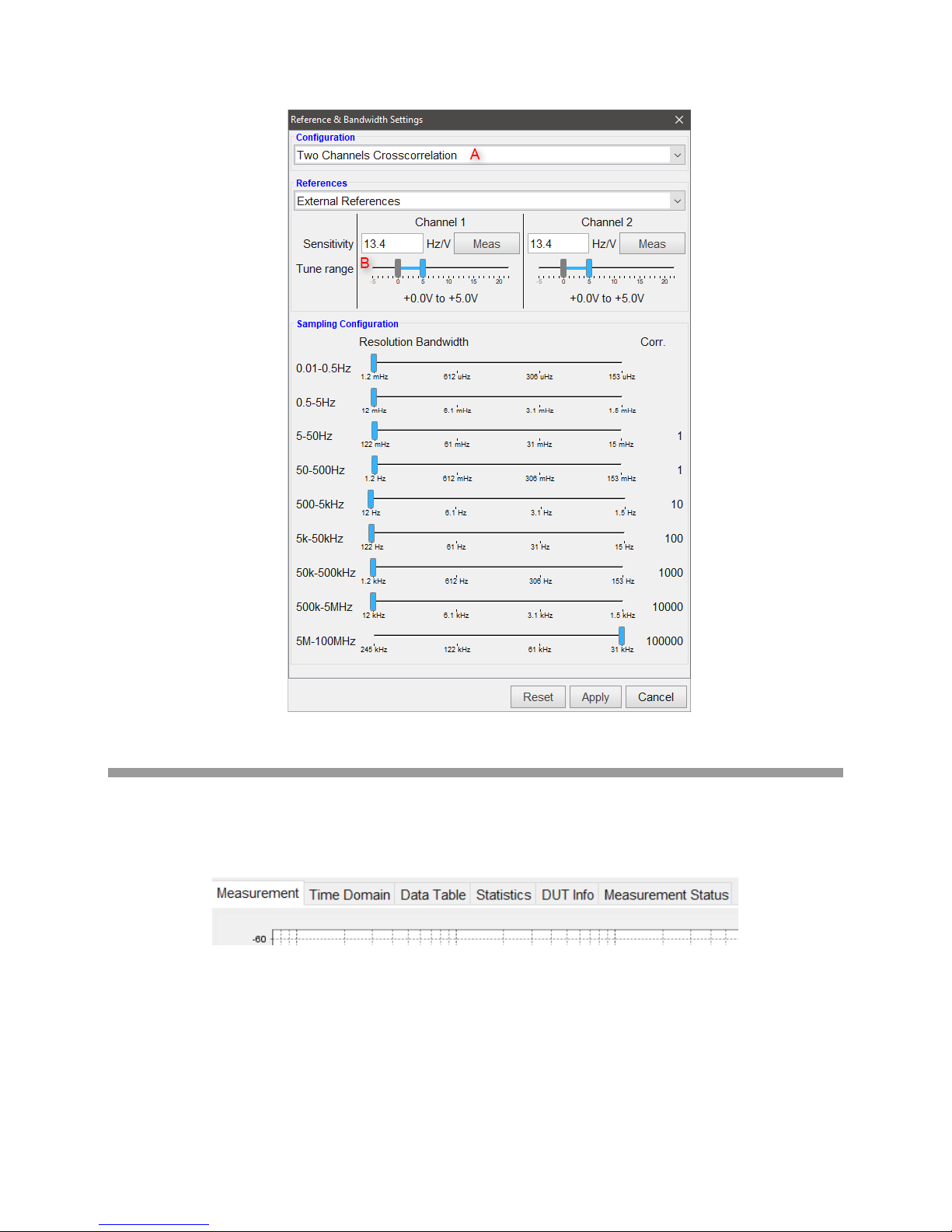
Figure 24: Absolute Phase Noise measurement of a pulsed signal

6.4.4 The Plot Window Tabs

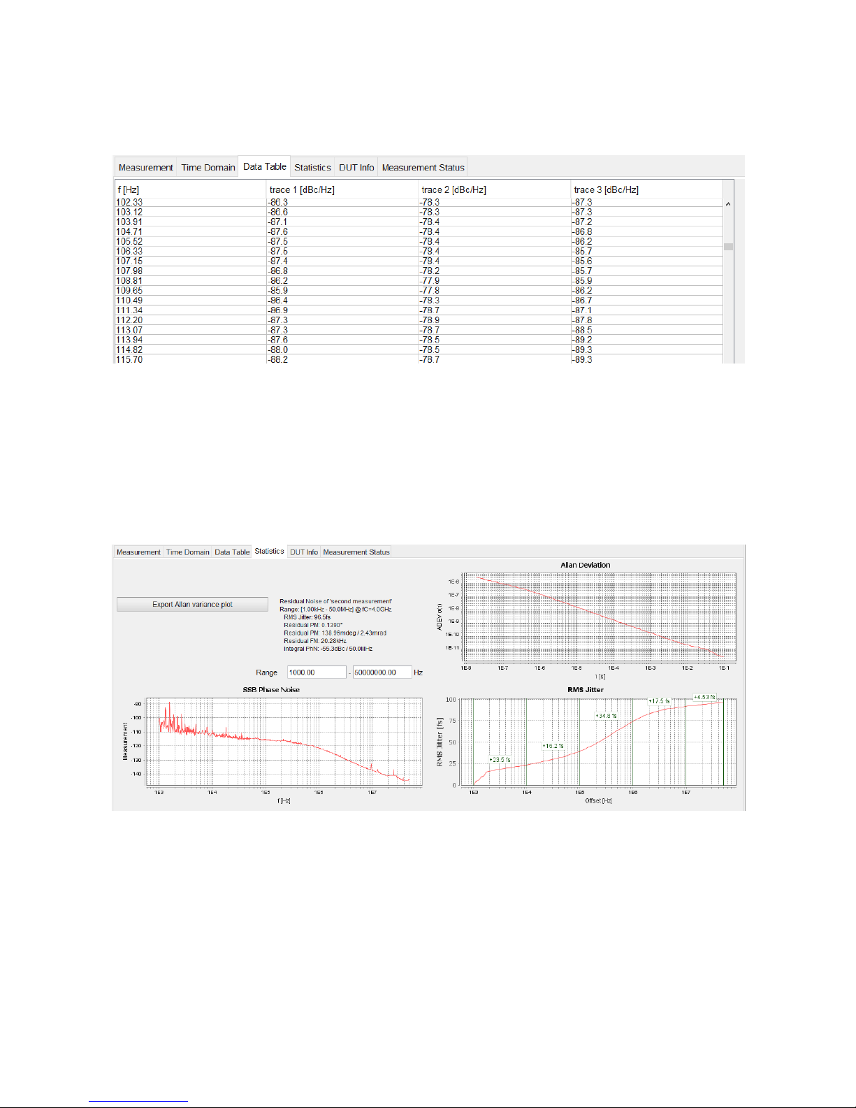
The plot window is comprised of six tabs: Measurement, Time Domain, Data Table, Statistics, DUT Info,
and Measurement Status:

Figure 25: Plot Window tabs

The Measurement tab is the main tab to display frequency domain results like phase noise plots.
The Time Domain tab is used to provide time domain measurement information during idle state

(frequency and power detection, calibration), and during the measurement process (locking, and data
acquisition). During the actual measurement, time samples of the noise voltage are also displayed in this
tab.

35 7000 Series User Manual September 2017



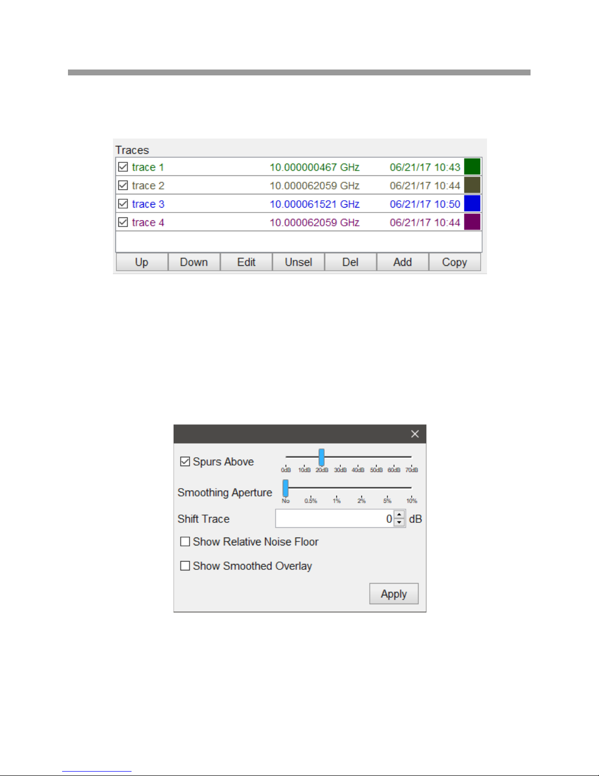
The Data Table tab displays the noise measurement data for all selected traces as a data table. This
table can also be exported to a file (various formats) with Plot

Figure 26: Data Table tab

Save.

The Statistics tab (as shown in Figure 27) provides additional statistical information such as integrated

RMS jitter, integral phase noise, residual FM/PM, Allan deviation, and a RMS jitter figure that plots RMS
jitter vs. offset frequency.

After each correlation the latest measurement is updated in the plot window. The Statistics tab displays
the information for the currently selected trace, or, if no trace is selected, for the first trace in the trace list.

Figure 27: Statistics tab

The DUT Info tab constantly monitors the DUT CW frequency and power while in idle mode and also

shows the tuning voltage of internal references during the measurement process. The values are updated
approximately once per second, while in GUI idle state.

The Measurement Status tab prints status and error messages that help the user to verify the
measurement process.

36 7000 Series User Manual September 2017

6.4.5 List of Traces

The list of traces is used to save and post-process acquired traces. The trace functions can be accessed
from the buttons located below the Traces window as shown below.

Figure 28: List of traces

6.4.5.1 Up and Down Buttons

Individual traces can be moved up and down by pressing the Up and Down buttons, respectively. The
ordering of the traces in the list affects the order in which they are drawn in the plot.

6.4.5.2 Edit Button

Selected traces can be edited with Edit button that opens the window shown below.

This dialog modifies all currently selected traces. It also sets the default parameter for future traces. The
following functions can be applied:

1. Completely remove or show detected spurious signals that are above a user-set threshold. See
section 6.4.7.3 for further information about displaying spurs.

37 7000 Series User Manual September 2017

Figure 29: Trace Edit dialog

2. Apply video averaging (smoothing) to the trace with user-set smoothing aperture.

3. Shift trace by a user specified number of decibels (up or down).

Enable or disable the display of the relative noise floor and a smoothed overlay of the trace. Changes are
immediately applied to the traces. The Apply button confirms and closes the window.

6.4.5.3 Selecting and Unselecting Traces (Unsel Button)

A single click on the line representing a trace will select that trace. The selected trace will be drawn as
thick line in the plot. Multiple traces can be selected or deselected by holding the Ctrl key, while clicking on
the traces. All traces will be unselected by clicking the Unsel button.

6.4.5.4 Delete Traces

Selected traces can be removed from the trace list by clicking on Del button, or by pressing the Delete
key.

6.4.5.5 Add Button

The current measurement trace (red trace) can be stored in the trace list by clicking on the Add button.
The stored trace is named with “trace <i>” (where <i> is the smallest number not already taken by another
trace). Additional information, such as DUT frequency, number of correlations, and time and date of
measurement are included in the trace list.

Each trace can be renamed by double-clicking on the corresponding trace name and typing in the new
trace name.

6.4.5.6 Copy Button

Use the Copy button to create identical copies of the selected traces.

6.4.5.7 Modify Color of Traces

Individual trace colors can be assigned to traces, by clicking on the color box on the right of the line in the
trace list and selecting the desired color from the color dialog. Traces stored in the list can be made
invisible in the current plot window by un-checking the check-box to the left of the trace name.

38 7000 Series User Manual September 2017

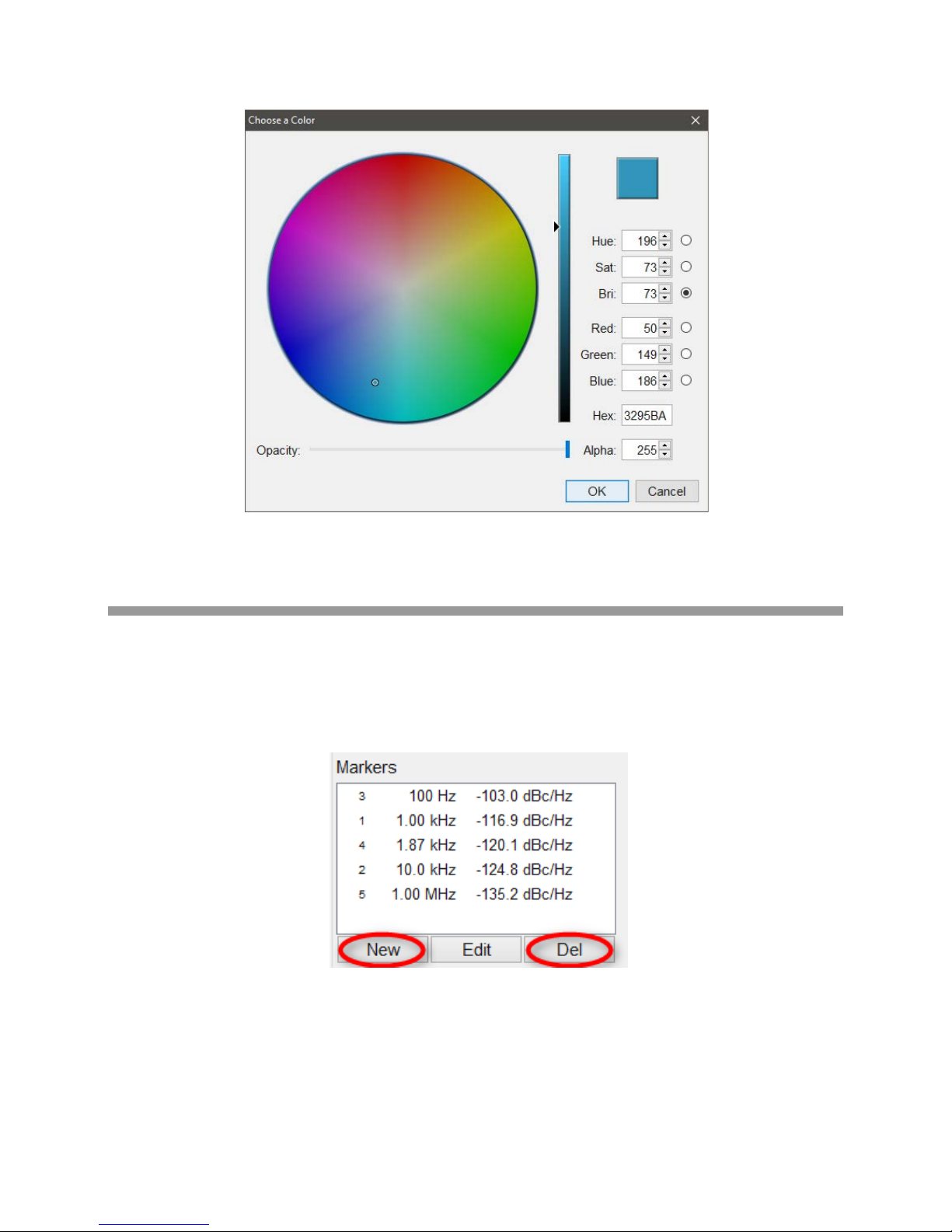
Figure 30: Trace color dialog

6.4.6 The Marker Window

Multiple noise markers can be applied within the plot window. To add a new marker, press the New
button, as shown below, and move the mouse within the plot window.

The marker will follow the active or selected trace. The markers are globally defined and not attached to a
particular trace. That means that by selecting another trace, the markers are shown for that specific trace.

39 7000 Series User Manual September 2017

Figure 31: Noise marker dialog

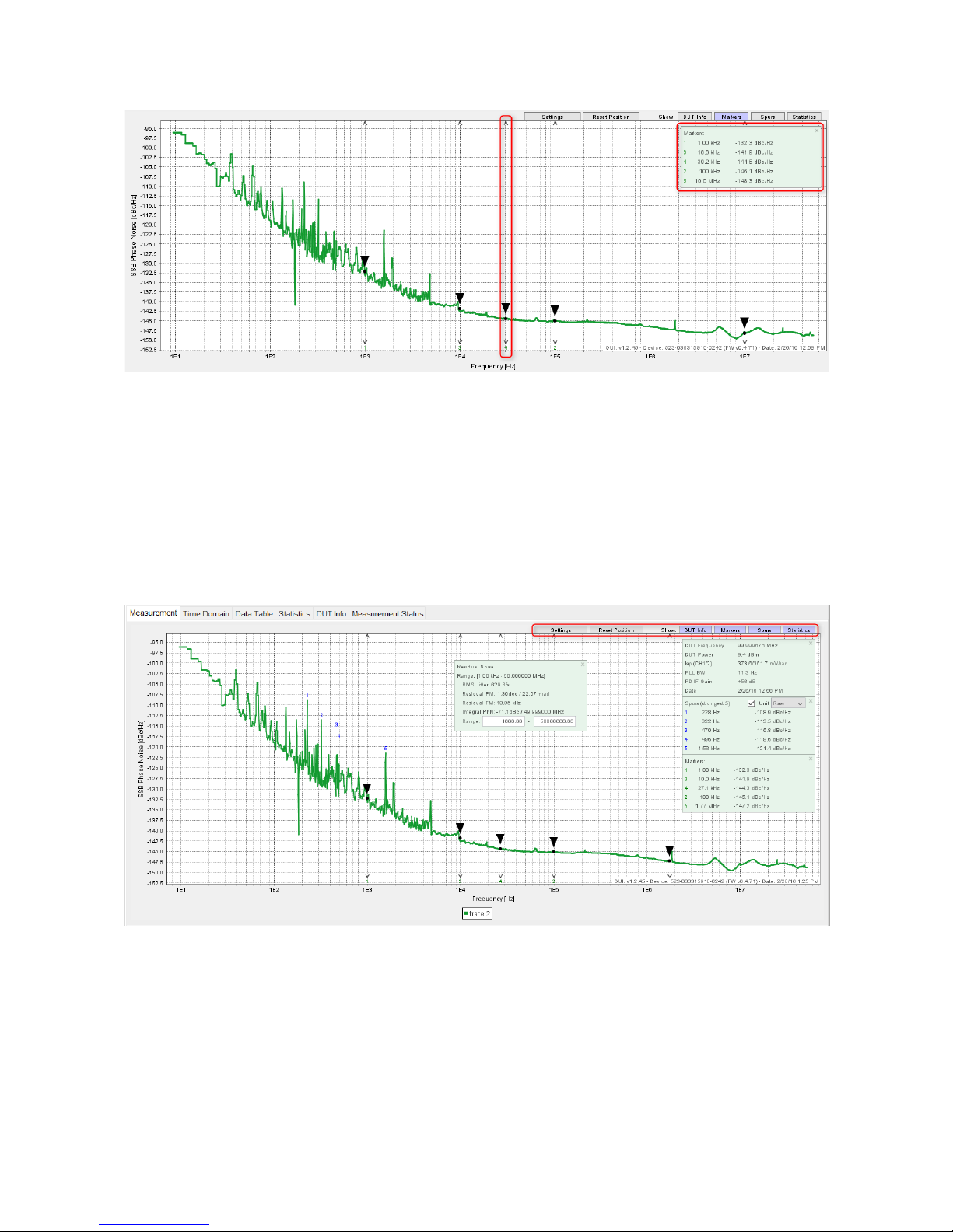
Figure 32:2 Plot window wit h multiple mar k e r s and the Marker list displayed

6.4.6.1 New Markers

After clicking the New button, the marker mode is activated. In this mode, a marker will follow your cursor
in the plot. The marker can be set with a single left click. The marker will then appear in the marker list and
the marker mode is deactivated again. The marker mode can also be left by pressing the Escape key on
the keyboard. Once a marker is placed, it can be moved by drag & drop and the corresponding phase
noise value is displayed in the windo w, as sho wn in Figure 32.

Figure 33: Plot area with statistical calculations, Marker list, Spur list and DUT Info displayed

6.4.6.2 Editing and Deleting Markers

Markers can be removed by selecting them in the markers list and clicking on the Del button. A selected
marker can be set to a precise offset frequency by clicking the Edit button and entering the desired value
by keyboard.

40 7000 Series User Manual September 2017

6.4.7 Plot Windows

There are several buttons in the upper right corner of the plot (marked red in the figure), as shown in
Figure 33.

6.4.7.1 Settings Button

With the Settings button, the Plot Settings dialog is opened, as shown in Figure 34. In this dialog, the
following general plot settings can be changed:

1. Assign a title to the plot

2. Change font size and legend labels

3. Change plot window background and grid color

4. Modify X and Y scales, labels, and units.

Changes are immediately applied to the traces. The Reset button allows resetting to default values.

6.4.7.2 Reset Position Button

If enabled, spur/marker lists, the RMS jitter, residual phase error, the residual FM, and the integral phase
noise are displayed for the selected trace as small windows inside the plot area, as shown in Figure 33.
The windows can be dragged around with the mouse pointer. To reset their position, click on the Reset
Position button. This will put all windows to the default location.

6.4.7.3 DUT Info, Markers, Spurs, Statistics button

The windows can be activated either in the plot settings dialog, or via the buttons in the upper right corner
of the plot. Windows can also be removed from the plot area by pressing the small "x" in the upper right
corner of the respective window. The windows have specific functionalities as well.

The DUT Info window shows information about the currently selected trace, including DUT power,
frequency, and measurement type. Also measurement specific parameters, such as PLL bandwidth,
selected IF gain and time stamp are displayed here.

The Spur window shows a list of the five strongest displayed spurs of the currently selected trace. This
window also provides the options to show or hide the spurs and select the spur display mode. The spur
display mode "Raw" shows the spurs exactly as measured. The spur display mode "1 Hz Eq." shows the
spurs as a 1 Hz wide spur with bandwidth adjusted power.

The Marker window shows a list of all markers with the values of the currently selected trace at the marker
offset frequencies.

The Statistics window shows statistical parameters of the currently selected trace, such as jitter, residual
FM, or integral phase noise. The integration range for the calculations can be adjusted in this window.

41 7000 Series User Manual September 2017

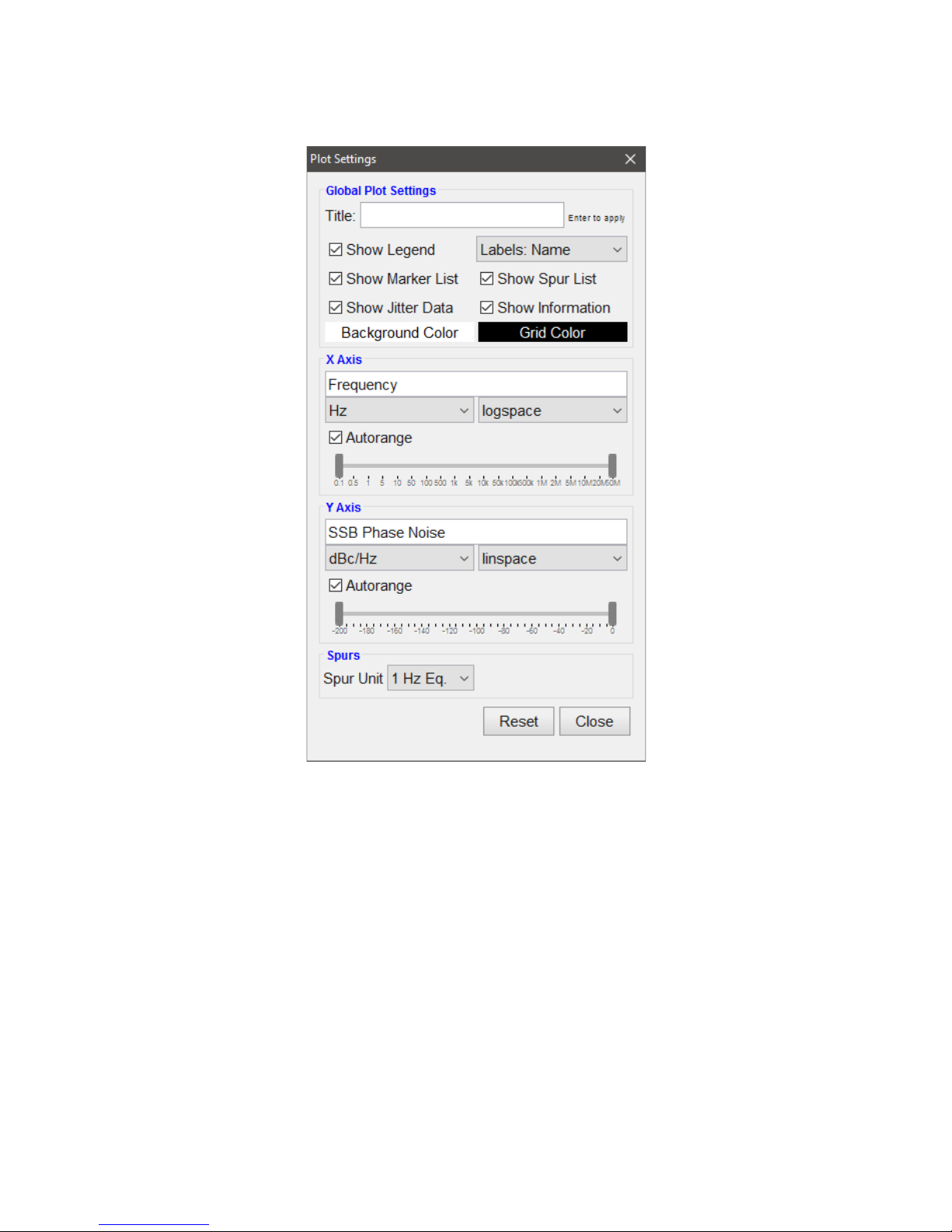
Figure 34: Plot Settings dialog

6.4.7.4 Additional Functionality

Within the plot window, you can also

i. Move marker: Click on the marker at any vertical point, and at the exact horizontal position of the

marker, to drag it horizontally to the desired position.

ii. Zoom in: Click with the mouse in the upper left corner of the desired zoom window and draw the

window. Release the mouse button to perform the zoom.

iii. Zoom out: To fully zoom out again, click on the plot window, move the mouse pointer to the upper

left, and release the mouse button again.

iv. Right click: Use the right mouse button on the plot area to print, save, and copy the plot (see

Figure 35).

42 7000 Series User Manual September 2017

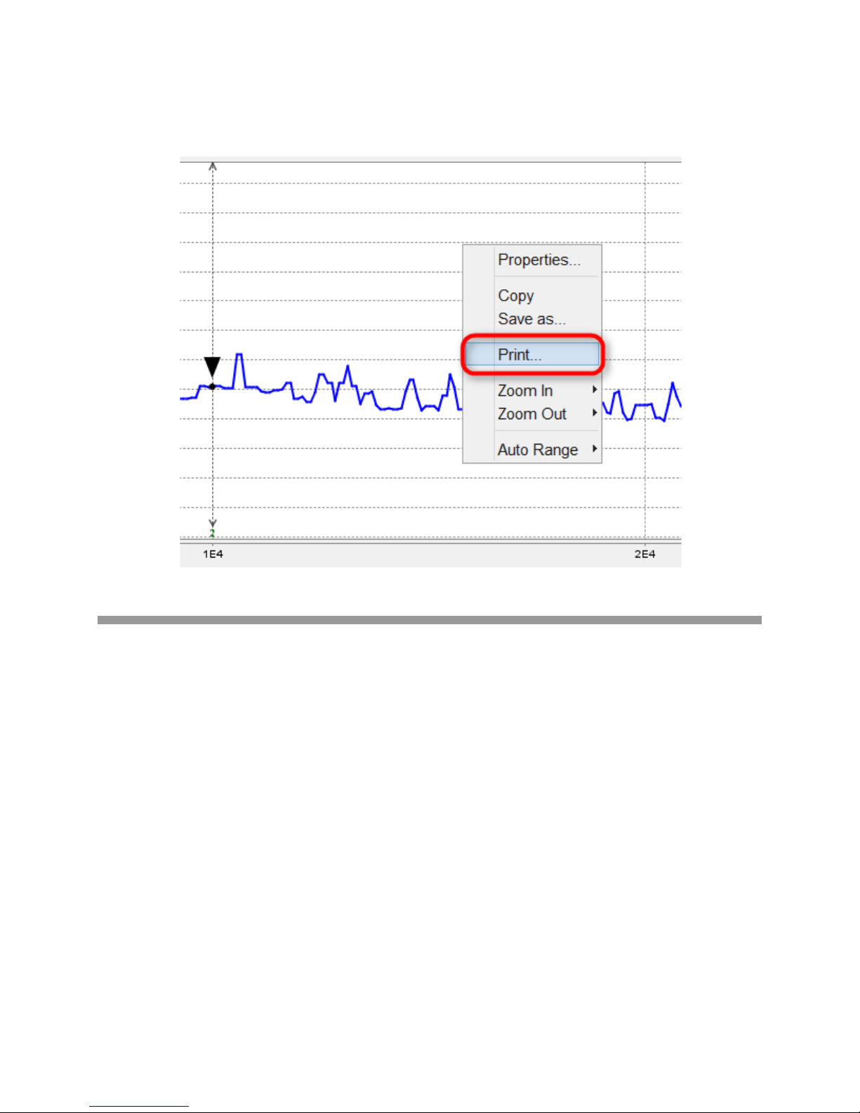
Figure 35: Zoomed-in trace and the Print option

6.4.8 Saving and Loading Traces

Traces can be exported and saved in various file formats through the Plot  Save Trace(s) menu. The
following formats are available:

• ASCII data of the selected trace in CSV format

• Microsoft Excel™

• Matlab™ Data File

• Plot win dow in PNG format

• All traces in the 7000 Series format (.apph) can be loaded into the GUI

Traces can be imported if they were previously saved in the 7000 Series internal format. Use the Plot 
Load Trace(s) menu. Select the 7000 Series file to import and then confirm by clicking the Open button.

43 7000 Series User Manual September 2017

6.5 General Measurement Settings

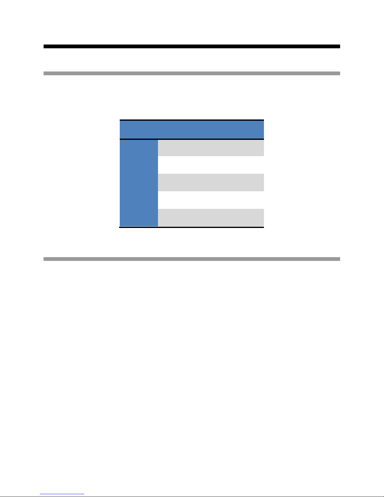
6.5.1 Number of Data Points per Trace

By default, the number of points displayed in every trace depends on the Start and Stop offset frequency
(see Table 1).

Start / Stop 10 kHz 100 kHz 1 MHz 50 MHz

0.1 Hz

1 Hz

10 Hz

100 Hz

1 kHz

Table 1: Displayed number of points per trace

6.5.2 Measurement Time (using GUI)

The measurement time required by the 7000 Seri es depends on several parameters. The total
measurement time consists of the setup time, sampling time, and post-processing time.

6.5.2.1 Setup Time

The setup time largely depends on the user settings and reference sources used. Very low noise

1250 1500 1750 2150

1000 1250 1500 1900

750 1000 1250 1650

500 750 1000 1400

250 500 750 1150

references tend to have a small tuning sensitivity and bandwidth. With narrower loop bandwidths, the
locking process takes longer. The setup time also depends on the measurement frequency and includes
performing calibration steps.

6.5.2.2 Sampling Time

The sampling time depends on the selected frequency offset range and the number of samples taken
(RBW). With a larger RBW, the ability to distinguish spurious content is reduced, however the sampling
time decreases. The number of measurement points per trace varies depending on the selected RBW.

44 7000 Series User Manual September 2017

6.5.2.3 Post-Processing Time

The post-processing time is used to process and visualize the measured data. The post-processing time
depends upon the performance of the computer on which the remote client software is running, and the
interface between 7000 Series and PC. LAN is generally faster than USB.

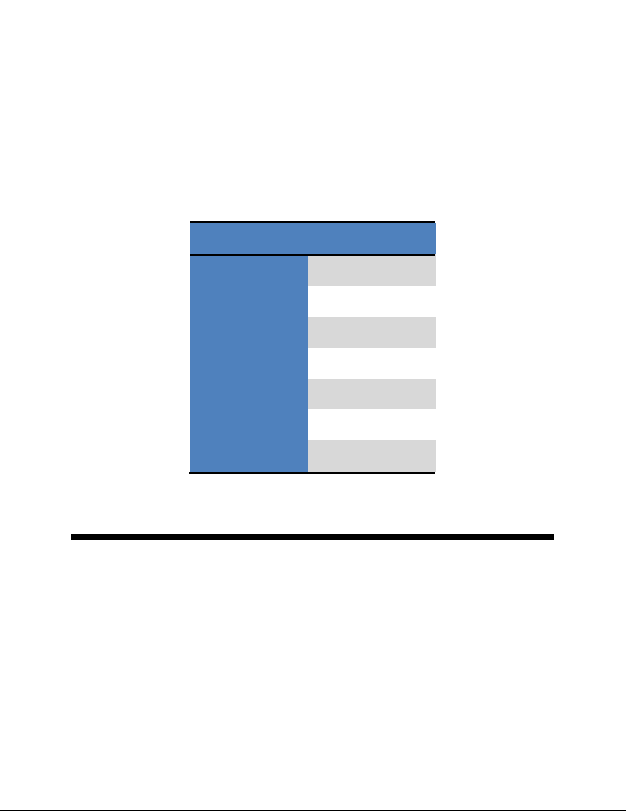
The typical measurement times per average / correlation (includes sampling and post-processing time,
default RBW) is shown in Table 2.

Start Frequency [Hz] Measurement Time [s]

0.01 Hz

0.1 Hz

1 Hz

10 Hz

100 Hz

1 kHz

10 kHz

Table 2: Typical measurement time for 7000 Series

6.6 Additive Phase Noise Measurement

450

51

9.3

5.0

3.3

3.3

3.3

The Additive Phase Noise measurement tab provides single-channel or two-channel cross-correlation,
additive phase noise measurements. It supports measurements of active or passive, not self-oscillating
devices such as amplifiers in linear and non-linear operation or even frequency-translating devices such
as mixers, frequency multipliers or dividers.

45 7000 Series User Manual September 2017

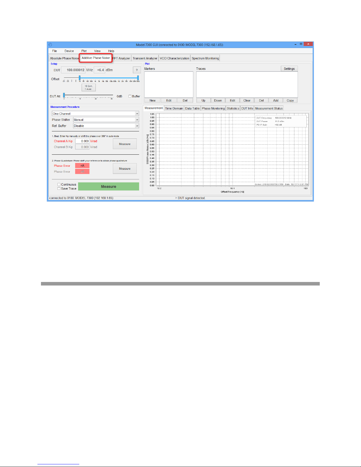
Figure 36: Additive Phase Noise measurement tab (blank)

The measurement principle is based on the assumption that the phase noise of the stimulating signal for
the DUT (external reference source) is completely cancelled out when manually adjusted to phase
quadrature. For the measurement setup, an external phase shifter and power splitter is required for each
measurement channel. A suitable external low-noise reference source (stimulus) must be used.

Click on the question mark button to display a schematic diagram that shows what the measurement
setup should look like for the currently set configuration.

6.6.1 Measurement Procedure

Before starting the calibration and measurement procedure, some parameters must be configured. Firstly,
select single-channel or two-channel measurement.

Next, select what kind of external phase shifter is deployed. Any phase shifter that does not excessively
contribute noise such as digital or mechanically tuned models is suitable. Models that are tuned via an
analog voltage can be supported by the 7000 Series GUI.

46 7000 Series User Manual September 2017

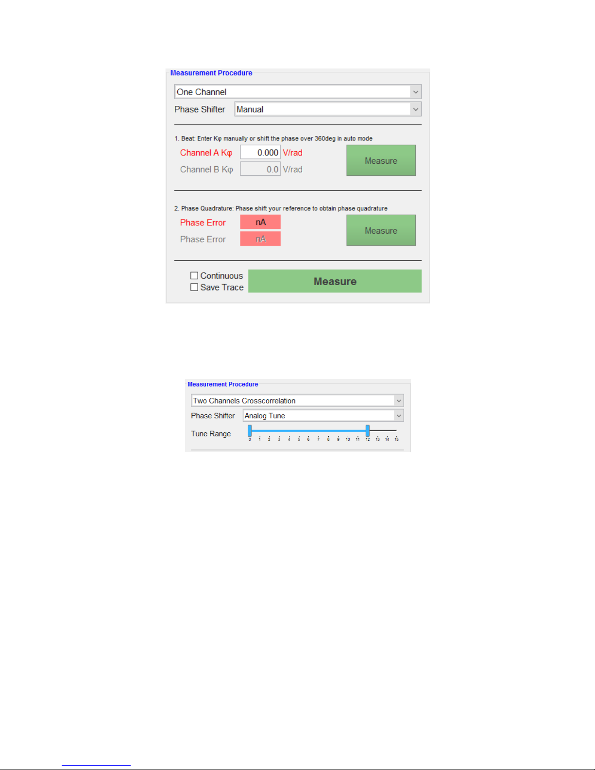
Figure 37: Measurement Procedure dialog

The drive level at both of the reference inputs as well as the DUT input, should be 10 dBm or higher.
Usually, this can be achieved with the configuration of the oscillator and the measurement setup itself.

Figure 38: Tuning dialog

The measurement procedure to perform an additive measurement consists of three steps:

1) Determine the phase detector constant. Press the Measure button in step 1.

a. If the phase shifter option "Automatic" is selected, the phase shifter does not have to be

operated for this step. The constant will be automatically determined and can be
confirmed by pressing the Confirm button.

b. Mechanically or digitally tune the phase shifters to provide at least 180 degrees of phase

shift in order to derive the phase detector constant.

c. If “Analog Tune” is selected and voltage controlled phase shifters are used, then this step

is performed automatically by the instrument, and can be omitted.

47 7000 Series User Manual September 2017

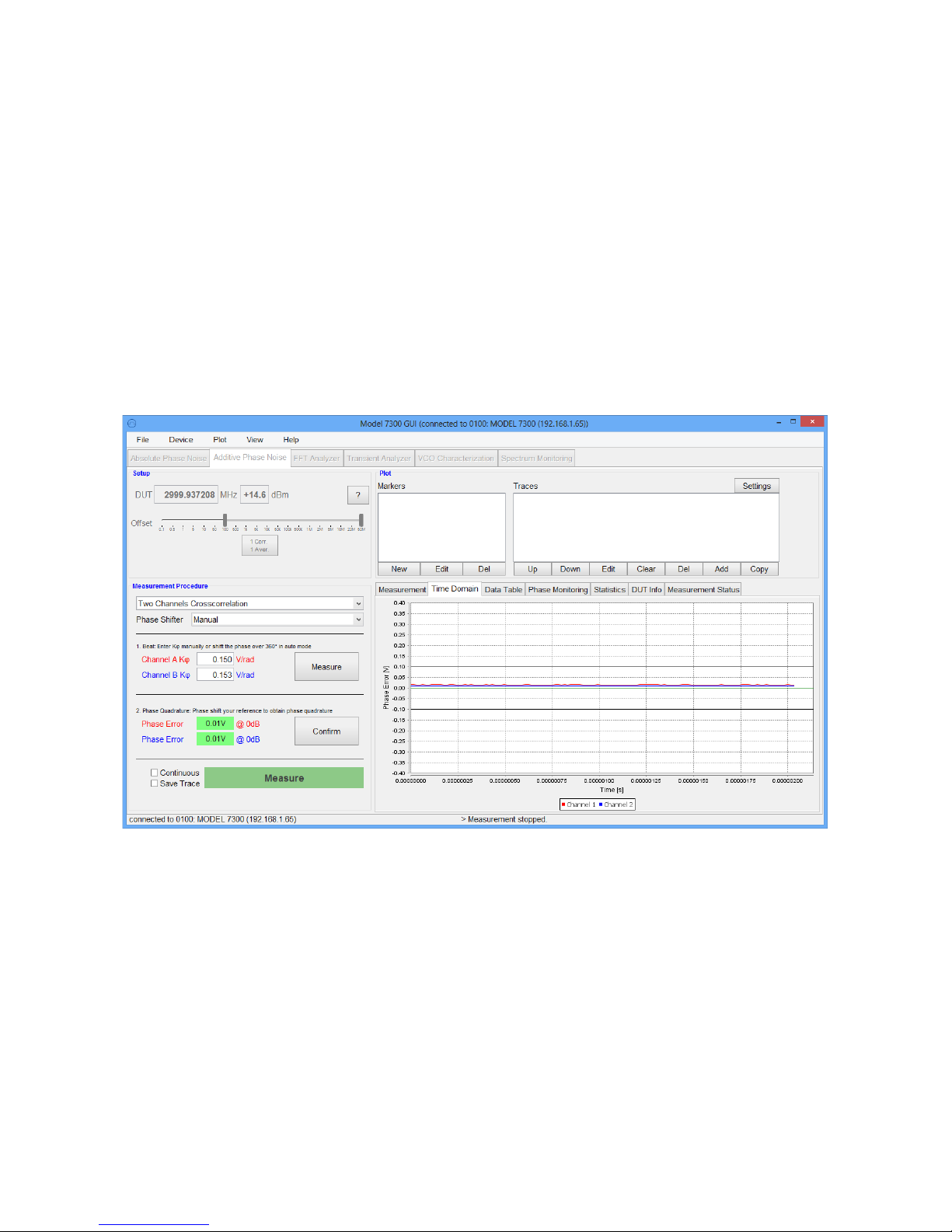
2) Once the phase detector constants are known, the phases must be adjusted to obtain phase
quadrature. Start this step by pressing the Measure button in step 2. Now, the phase difference
between the signal pairs at RF IN and REF IN (1 and 2) must be adjusted using the external
phase shifters to achieve approximate phase quadrature (90 degree phase difference), as shown
in Figure 39. The GUI shows a tolerance window of ±3 degrees. If “Analog Tune” is selected and
voltage controlled phase shifters are used, then this step is performed automatically by the
instrument and can be omitted.

3) Finally, the actual measurement can be initiated by pressing the green Measure button, as shown
in Figure 40. Measurement can be stopped and restarted without need of performing step 1 and 2
for every measurement cycle unless there are changes in the measurement setup.

Figure 39: Additive Phase Noise Measurement tab during step 2, adjusting the phase to quadrature

48 7000 Series User Manual September 2017

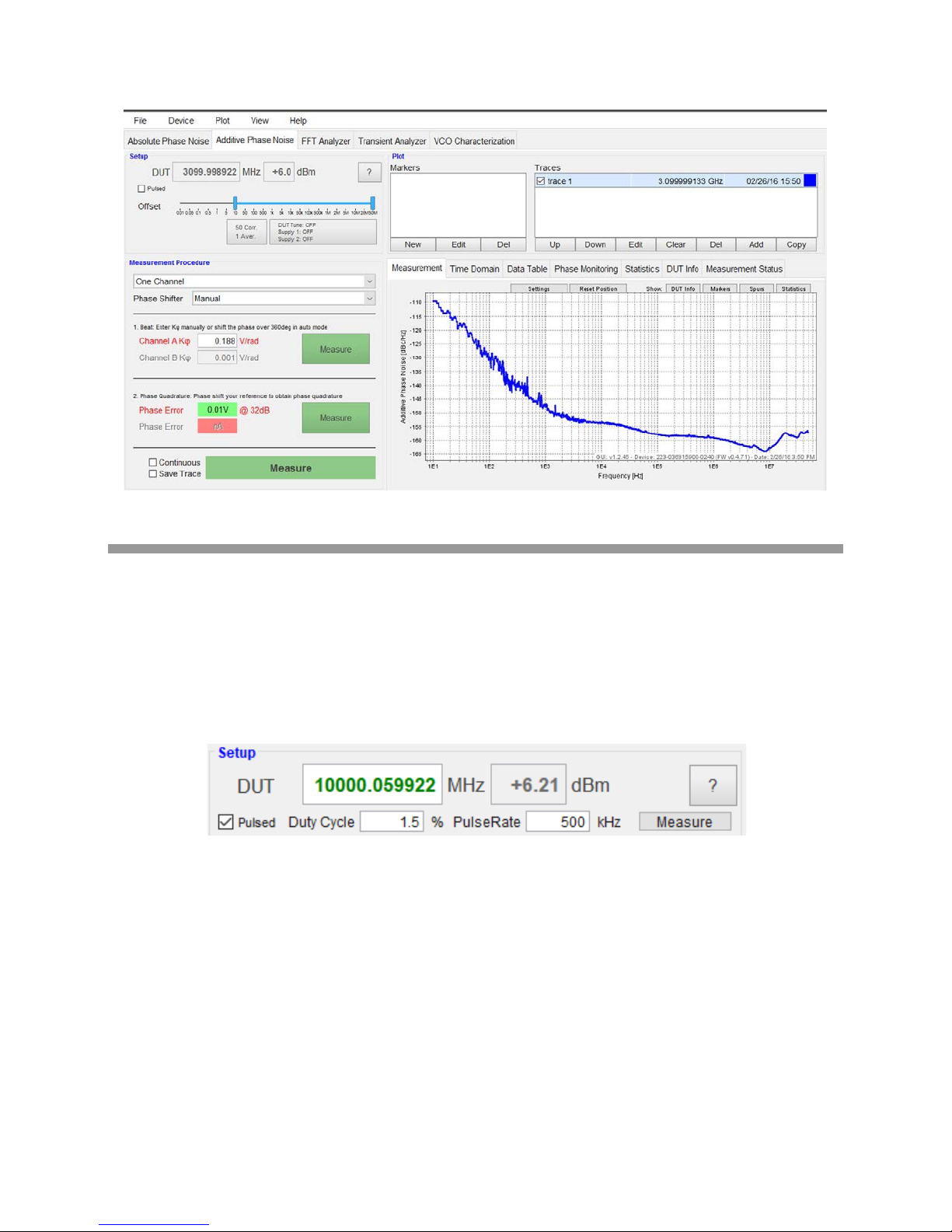
Figure 40: Additive Phase Noise Measurement tab after a measurement cycle

6.6.2 Additiv e Ph ase Noise of a Pulsed Signal (with Option PULSE only)

To configure the 700 0 Seri es for additive pulse modulated signals, the Pulsed checkbox in the setup
region of the additive phase noise tab must be enabled. Upon activation, some pulse modulation specific
input controls are displayed (see Figure 41). The duty cycle and pulse rate of the modulated signal must
be entered. This can be done either manually or automatically by detection. Press the Measure button on
the right side of the pulse row to automatically detect the pulse modulation parameters.

Figure 41: Pulse Modulation specific input controls in the Additive Phase Noise tab

The measurement procedure is identical to the procedure for unmodulated signals. First, the phase
constant has to be determined by shifting the phase from 0° to 360° between the DUT and REF port.
Second, the phase must be adjusted to ensure the two signals are in quadrature. For the pulsed signals,
the beat signal will be a flat line when this is achieved. Third, the measurement can be initiated with the
Measure button and will be displayed up to the set pulse rate (see Figure 42).

49 7000 Series User Manual September 2017

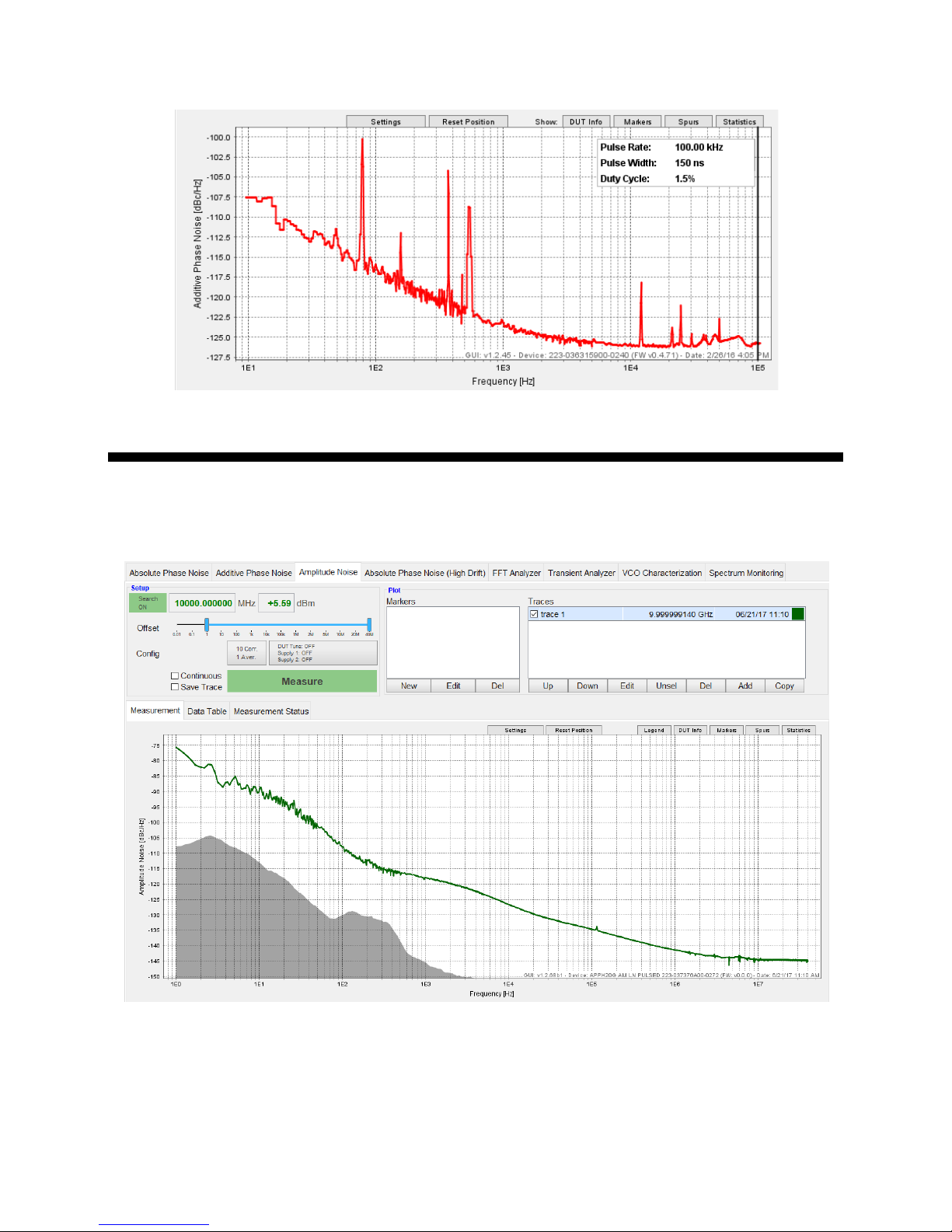
Figure 42: Additive Phase Noise measurement of a pulse modulated signal

6.7 Amplitude Noise Measurement

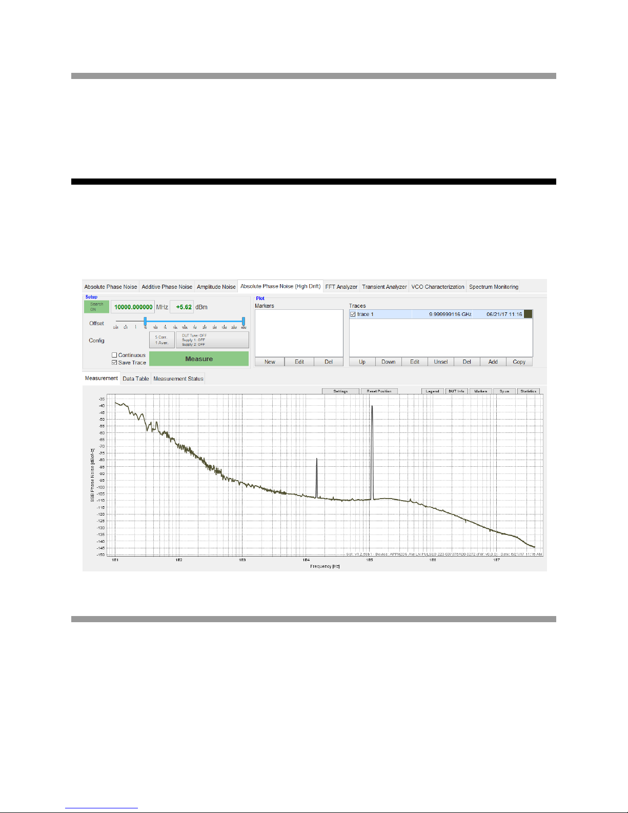
From an interface standpoint, the Amplitude Noise measurement tab is similar to the Absolute Phase
Noise tab (see section 6.4). This measurement mode can process CW and pulse modulated signals.

The device under test’s (DUT's) signal frequency and power is detected and the amplitude noise of the
signal in the specified offset frequency range is analyzed. The measurement principle is based on a digital
amplitude demodulation in combination with a two-channel cross-correlation system.

50 7000 Series User Manual September 2017

Figure 43: Amplitude Noise measurement

6.7.1 Measurement Procedure

Connect your signal source to the RF input port of the DUT section on the front panel of the instrument.
Choose the frequency offset range and number of averages and correlations. Start the measurement by
clicking on the Measure button. Intermediate results will show up with every completed correlation and the
final result will be displayed after the measurement has finished.

6.8 Absolute Phase Noise (High Dri f t )

The High Drift Absolute Phase Noise measurement tab has a similar appearance to the Absolute Phase
Noise tab. The difference is only the measurement principle. While the standard absolute phase noise
mode is based on the phase discriminator method, the high drift absolute phase noise mode is based on a
digital phase demodulation in combination with a two-channel cross-correlation system.

Figure 44: Absolute Phase Noise (High Drift) for a frequency modulated signal (110 kHz modulation frequency, 100 kHz

6.8.1 Measurement Procedure

Connect your signal source to the RF input port of the DUT section on the front panel of the instrument.
Choose the frequency offset range and number of averages and correlations. Start the measurement by
clicking on the Measure button. Intermediate results will show up with every completed correlation and the
final result will be displayed after the measurement has finished.

51 7000 Series User Manual September 2017

deviation)

6.9 Transient Analyzer Measurement

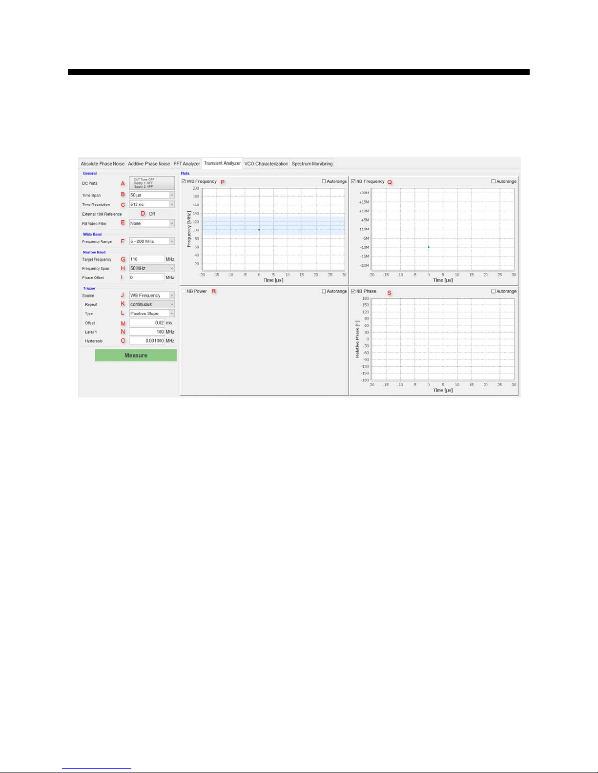
The Transient Analyzer tab provides frequency, phase, and amplitude versus time measurements. The
sampling period can be chosen down to 16 ns, allowing the user to look at fast frequency transients and
modulations.

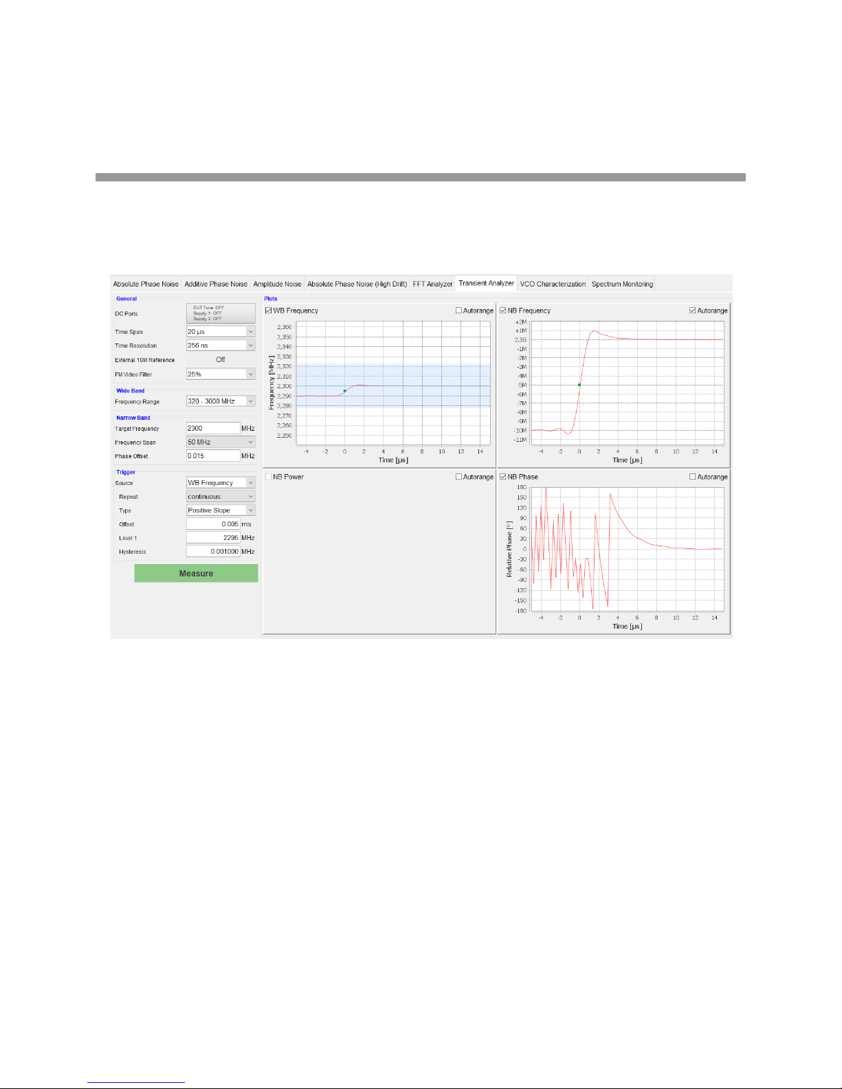
Figure 45: Transient Analyzer tab

After switching into the corresponding tab, the GUI appears as shown in Figure 45.
The transient analysis measurement mode offers the measurement of four parameters against time. There

are two available channels that can be configured separately to measure one of the following parameters:

1. Wide band frequency (WBF): The DUT signal frequency is directly divided, allowing it to cover a
wide frequency range of several GHz, depending on the selected range. This parameter requires
a full channel.

2. Narrow band frequency (NBF): This mode mixes the input signal with a selectable center
frequency, resulting in a low frequency beat. This allows for measurements with higher accuracy
and a frequency range up to 100 MHz. This parameter requires one channel, but can share this
channel with the narrow band phase par ameter.

3. Narrow band power (NBA): The narrow band principle also allows measuring the amplitude of
the signal. The result is shown as relative power in dB (relative to the highest data point in the
measurement). This parameter requires a full channel.

4. Narrow band phase (NBP): This mode provides the measurement of phase versus time,
referenced to the narrow band target frequency. This parameter requires one channel, but can
share the channel with the narrow band frequency parameter.

52 7000 Series User Manual September 2017

Apart from the restrictions mentioned above, the parameters can be selected freely. It is therefore
possible to measure WBF, NBF and NBP at the same time. Alternatively, a measurement can cover NBF,
NBA, and NBP. It is, however, not possible to measure all four parameters at the same time.

6.9.1 Measurement Procedure

Connect your signal generator to the DUT input connector of the 7000 Series . Choose the parameters to
be measured by activating them in the plot region (P, Q, R, and S).

Figure 46: Transient Analysis of a frequency change from 2.29 GHz to 2.3 GHz

Start the measurement in continuous mode by selecting continuous mode in the measurement drop-down
menu (K) and then click on the green Measure button. The measurement will now continuously run. You
can change the sampling configuration by adjusting the Time Resolution (C) between 16ns and 50 ms,
and the Time Span (B) between 10 µs and 1 min. Higher values in the time resolution will provide better

frequency accuracy at the cost of a lower sampling rate. By default, the plot will be scaled to show the
whole selected frequency range. The y-axis scaling can be automatically adjusted after every
measurement by enabling the Autorange option in the upper right corner of the plots. Moreover, you can
define a zoom area by holding down the left mouse button and dragging down and right. Reset the plot
axes by holding down the left mouse button and dragging up and left.

For the wide band measurement, select the Frequency Range of the signal with the drop down menu (F).
For the narrow band measurement, select the Target Frequency (G) and Frequency Span (H). The narrow
band phase measurement uses the target frequency as reference. A reference Phase Offset can be set by
adjusting the value in the text field (I).

53 7000 Series User Manual September 2017

An FM Video Filter (E) can be set to smooth the result for both narrow and wide band measurement.

Supply and tune voltages: The supply and DUT tune ports can be set directly in the Transient Analyzer
tab by clicking on the button (A).

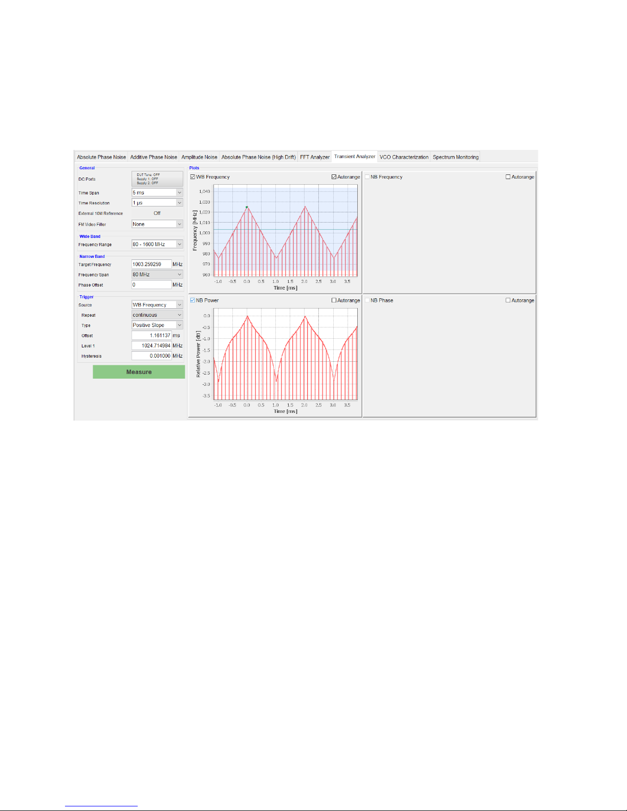
Figure 47: Analysis of a pulse modulated, chirping signal

Trigger System: The Trigger system enables access to a variety of trigger modes. To activate the Trigger

select the trigger Source as WB frequency, NB frequency or external (J and Figure 48) . T his wi ll v is ual ly
show the trigger configuration in the plot (in green). Select the trigger Type from the drop down menu (L).
Trigger types that can be chosen are:

Positive/Negative Slope triggers, for when the signal travels through a specific frequency (named Level 1)
in a selected positive or negative direction. The trigger position is visually shown with a green dot on the
plot. This dot can be dragged around with the mouse to change frequency and delay of the trigger.
Alternatively, the text boxes on the left can be used to manually insert specific values. Use the Enter key
to confirm. A Hysteresis can be set to minimize trigger events caused by noise in the signal.

Entering/Leaving Window triggers when the signal enters or leaves a selected frequency window defined
by two border frequencies (named Level 1 and Level 2). The trigger position is visually shown with a
vertical green line with two circles at the top and bottom. The frequency limits and delay of the trigger can
be changed by dragging the two dots or the vertical line. Alternatively, the text boxes on the left can be
used to manually insert specific values. Use the Enter key to confirm.

54 7000 Series User Manual September 2017

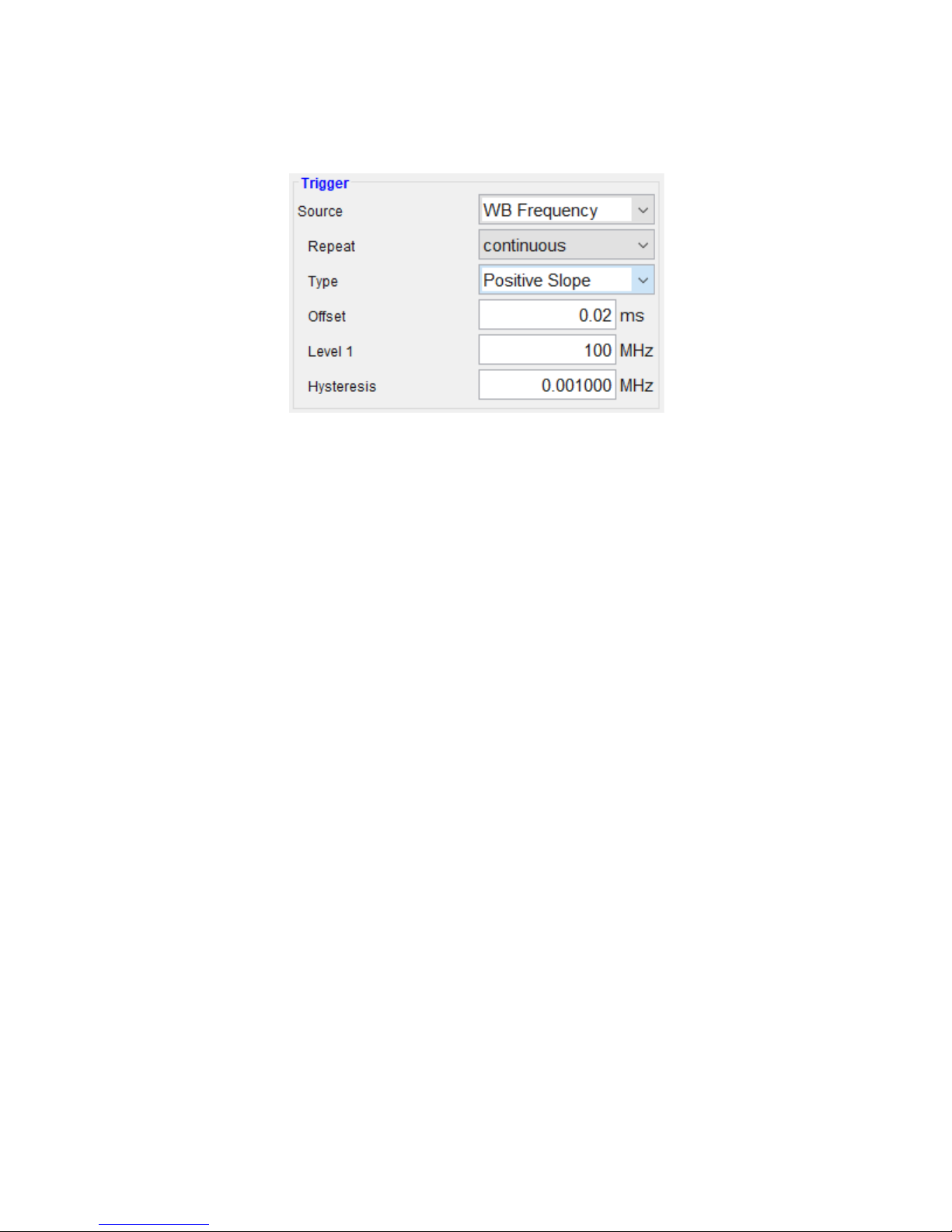
Figure 48: Trigger configuration dialog

The external trigger port is located on the rear panel of the 7000 Series and is marked EXT TRIG. The
trigger level is 1 V +/- 0.1 V, and can only distinguish between positive and negative slope. The window
trigger options are not available for external triggering.

External 10 MHz Reference By default, the frequency counter of the transient analyzer is referencing an
internal clock. It is possible to supply an external reference at 10 MHz to the REF IN 10 MHz port. To
activate the external referenc e, connect a 10 MHz reference to the REF IN 10 MHz port on the rear panel,
and activate the External 10M Reference checkbox (D) by clicking on the Off text. The text will change to
"Checking". This process can take a few seconds. If successful, the text background will turn green and
the text will change to "Locked" to indicate that the reference was detected and locked. If no valid
reference was detected, the background will turn red and the text will change to "Not Locked". After a few
seconds, the text will change to "Off" again.

55 7000 Series User Manual September 2017

6.10 FFT Analyzer Measurement

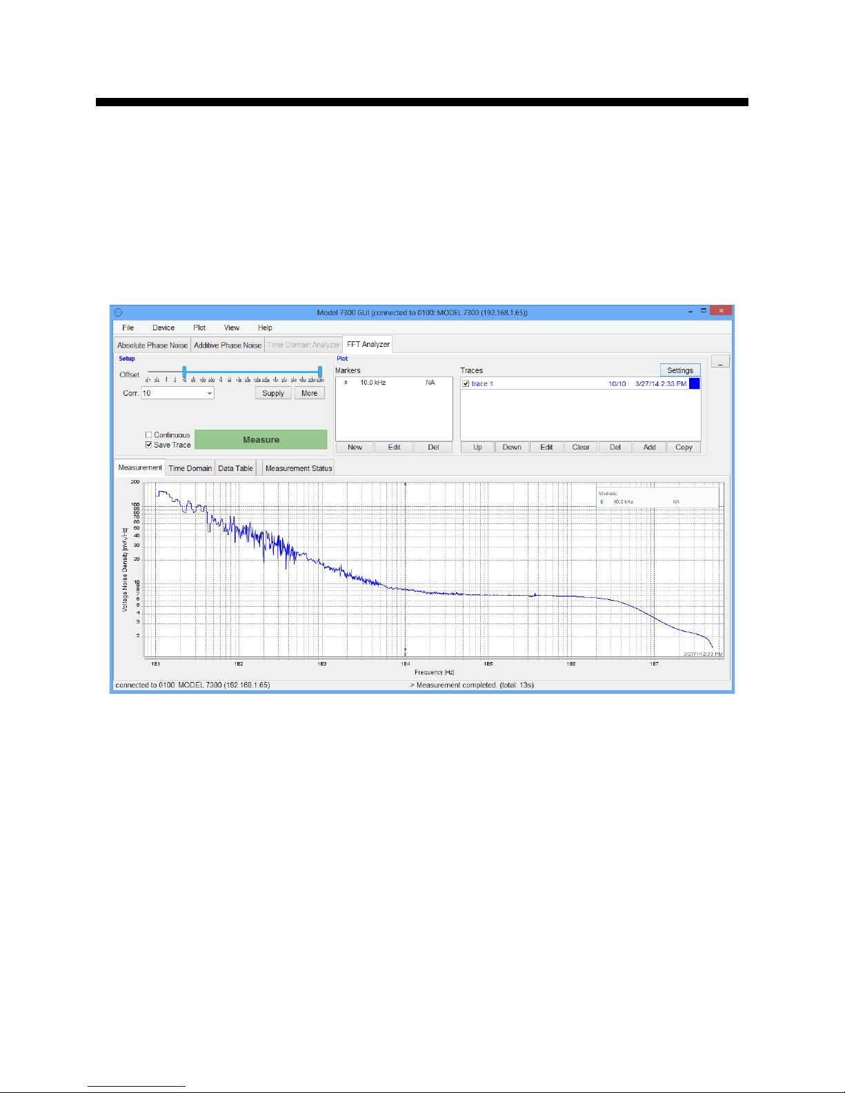
This tab is used to measure noise on one or two channels of the FFT analyzer. Connect the DUT to the
BASEBAND ports on the rear panel of the 7000 Series . To perform two-channel measurements, the
signal must be split externally and connected to both BASEBAND 1 and BASEBAND 2. For a single­channel measurement, only BASEBAND 1 is required. Select the frequency offset range and the number
of averages and correlations. Select either “Single Channel” or “Two channel cross-correlated”
measurement. Press the Measure button to run the measurement.

56 7000 Series User Manual September 2017

Figure 49: FFT Analyzer mode

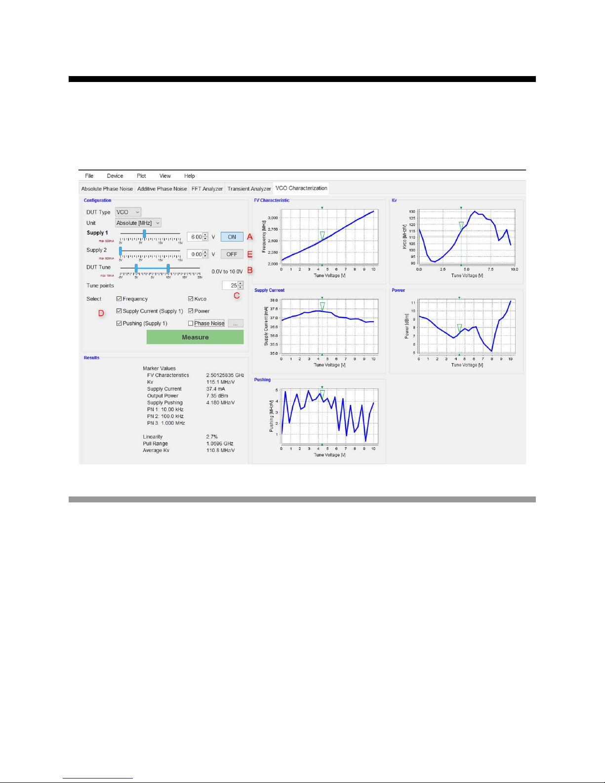
6.11 VCO Characterization

The VCO Characterization tab provides the ability to fully characterize a voltage controlled oscillator (VCO
or VCXO), including Kvco, current draw, power output, pushing and spot phase noise over a specified
control voltage range.

Figure 50: VCO Characterization tab

6.11.1 Measurement Procedure

Connect the VCO to the 7000 Series . Use the DC SUPPLY 1 port on the rear panel of the 7000 Series
as supply voltage, the DUT TUNE port on the front panel of the 7000 Series as control voltage and
connect the RF output of the VCO to the DUT RF IN port of the 7000 Series .

Next, select the supply in the VCO characterization tab and turn the Supply 1 output (A) on. Select the
tuning range of your VCO (B). The unused supply port on the rear panel can be used as additional voltage
and can be set accordingly (E). Choose the number of Tune points (C) for the measurement. Those points
will be equally distributed within the selected tune range. Individual measurement parameters can be
enabled/disabled by using the Select check-boxes (D).

A click on the green Measure button will start the measurement. The process will go through all tune
voltage points and measure the enabled parameters.

57 7000 Series User Manual September 2017

Every plot shows a single frequency marker that can be synchronously moved in all plots by dragging it
with the mouse on any of the displayed plots.

Additional information about the measurement is shown in the Results region below the Measure button.
First, the numeric marker values are displayed. Below the marker values, the linearity, pull range, and
average Kv of the measurement are displayed.

58 7000 Series User Manual September 2017

7 Remotely Programming t he 7000 Series

The 7000 Series can be remotely controlled via three independent, but functionally equivalent interfaces:
USBTMC, LAN, and (optionally) GPIB.

7.1 Access via LAN

The signal analyzer can be remotely programmed via a 10/100/1000Base-T LAN interface and LAN­connected computer using one of several LAN interface protocols. The LAN allows instruments to be
connected together and controlled by a LAN- based computer. LAN, and its associated interface
operations, are defined in the IEEE 802.2 standard.

The 7000 Series supports the fol lo wing LA N interface protocols:

1) Socket based LAN: proprietary function calls defined in the dynamic link library (DLL) provided
with the instrument. Used for general programming with the LAN interface under Windows
operating system.

2) VXI-11/SCPI (version 1999) commands (firmware 1.0 upwards)

3) Telephone Network (TELNET): TELNET is used for interactive, one-command-at-a-time
instrument control

For LAN operation, the instrument must be connected to the LAN, and an IP address must be assigned to
the instrument either manually or by using DHCP client service. Your system administrator can tell you
which method to use. (Most current LAN networks use DHCP.)

DHCP Configuration

If the DHCP server uses dynamic DNS to link the hostname with the assigned IP address, the hostname
may be used in place of the IP address. Otherwise, the hostname is not usable.

7.2 Using and Configuring VXI -11

The analyzer supports the LAN interface protocol described in the VXI- 11 standard. VXI- 11 is an
instrument control protocol based on Open Network Computing/Remote Procedure Call (ONC/RPC)
interfaces running over TCP/IP.

A range of standard software such as NI-VISA, or Agilent IO Config is available to setup the
computer/analyzer interface for the VXI- 11 protocol. Please refer to the applicable software user manual

59 7000 Series User Manual September 2017

and documentation for information on running the program and configuring the VXI-11 interface. The
program is used to configure the LAN client. Once the computer is configured for a LAN client, you can
use the VXI-11 protocol and the VISA library to send SCPI commands to the signal generator over the
LAN interface. Example programs are available upon request by contacting
[email protected].

VISA is an IO library used to develop IO applications and instrument drivers that comply with industry
standards. It is recommended that the VISA library be used for programming the signal source analyzer.
The NI-VISA and Agilent VISA libraries are similar implementations of VISA and have the same
commands, syntax, and functions.

7.3 Using the USB-TMC Interface with VISA

The USB (Universal Serial Bus) remote control system provides device control via USB, which is
equivalent to control via LAN
USBTMC-USB488 and US B 2.0

The 7000 Series models conform to USB Test & Measurement Class (USBTMC) protocol. This simplifies
instrument control considerably. Such devices behave like GPIB devices when communicating.

You must install the VISA Libraries on your PC in advance. The USB can identif y devices automatically,
so once you connect a USB cable to a target device, a dialog box will appear for USB device registration
on the host PC.

Please see the 7000 Se rie s Programmer’s Manual for detailed description of supported SCPI

or GPIB. Connection is made through an interface in compliance with

Type B: USB (USBTMC) interface port

7.4 Using the USB-TMC Interface with IVI Drivers

Please see the 7000 Se rie s Programmer’s Manual for detailed description of supported SCPI

60 7000 Series User Manual September 2017

commands.

commands.

7.5 Using the GPIB Interface

The GPIB interface operates with IEEE488.2 and SCPI. The instrument can be controlled by a GPIB
external controller. When controlling the 7000 Series using GPIB commands from the external controller
connected to the GPIB connector, the talker/listener GPIB address of the 7000 Series requires setting.
The default GPIB address of the 7000 Series is 1.

Please see the 7000 Se rie s Programmer’s Manual for detailed description of supported SCPI

commands.

61 7000 Series User Manual September 2017

8 Maintenance and Warranty Info rm at ion

8.1 Adjustments and Calibration

To maintain optimum measurement performance, the instrument should be calibrated every 24 months. It
is recommended that the instrument be returned to Berkeley Nucleonics or to an authorized calibration
facility. For more information please contact our Customer Service Department as indicated on
www.BerkeleyNucleonics.com.

8.2 Repair

The instrument contains no user-serviceable parts. Repair or calibration of the instrument requires
specialized test equipment and must be performed by Berk ele y Nucleon ic s or its authorized repair
specialists.

8.3 Warranty Information

All Berkeley Nucleonics instruments are warranted against defects in material and workmanship for a
period of two years from the date of shipment. Berk ele y Nucleo nics will, at its option, repair or replace
products that prove to be defective during the warranty period, provided they are returned to Berkeley
Nucleonics and provided the preventative maintenance procedures are followed. Repairs necessitated by
misuse of the product are not covered by this warranty. No other warranties are expressed or implied,
including but not limited to implied warranties of merchantability and fitness for a particular purpose.
Berkeley Nucleonics is not liable for consequential damages.

8.4 Equipment Returns

For instruments requiring service, either in or out of warranty, contact your local distributor or Berkeley
Nucleonics Customer Service for pricing and instructio ns befor e return in g your ins tr ument.

When you call, be sure to have the following information available:

• Model number.

• Serial number.

• Full description of the failure condition.

Note: Model and serial number can be found on the rear of the instrument, next to the power plug.

You will get a Return Merchandise Authori zat io n (RMA) num ber f rom Berk ele y Nucleo nic s , please put it
on the outside of the package.

Instruments that are eligible for in-warranty repair will be returned prepaid to the customer. For all other
situations the customer is responsible for all shipping charges. An evaluation fee may be charged for
processing instruments that are found to have no functional or performance defects.

62 7000 Series User Manual September 2017

For out of warranty instruments, Berkeley Nucleonics will provide an estimate for the cost of repair.
Customer approval of the charges will be required before repairs can be made. For instruments deemed
to be beyond repair, or in situations where the customer declines to authorize repair, an evaluation charge
may be assessed by Berkeley Nucleonics.

63 7000 Series User Manual September 2017