

Page 1

Page 2

Safety Summary
The following safety precautions apply to both operating and maintenance personnel and must be followed during all
phases of operation, service, and repair of this instrument.
Before applying power to this instrument:
• Read and understand the safety and operational information in this manual.
• Apply all the listed safety precautions.
• Verify that the voltage selector at the line power cord input is set to the correct line voltage. Operating the instrument
at an incorrect line voltage will void the warranty.
• Make all connections to the instrument before applying power.
• Do not operate the instrument in ways not specied by this manual or by B&K Precision.
Failure to comply with these precautions or with warnings elsewhere in this manual violates the safety standards of design,
manufacture, and intended use of the instrument. B&K Precision assumes no liability for a customer’s failure to comply
with these requirements.
2
Category rating
The IEC 61010 standard denes safety category ratings that specify the amount of electrical energy available and the
voltage impulses that may occur on electrical conductors associated with these category ratings. The category rating is
a Roman numeral of I, II, III, or IV. This rating is also accompanied by a maximum voltage of the circuit to be tested,
which denes the voltage impulses expected and required insulation clearances. These categories are:
Category I (CAT I): Measurement instruments whose measurement inputs are not intended to be connected to the
mains supply. The voltages in the environment are typically derived from a limited-energy transformer or a battery.
Category II (CAT II): Measurement instruments whose measurement inputs are meant to be connected to the mains
supply at a standard wall outlet or similar sources. Example measurement environments are portable
tools and household appliances.
Category III (CAT III): Measurement instruments whose measurement inputs are meant to be connected to the mains
installation of a building. Examples are measurements inside a building’s circuit breaker panel
or the wiring of permanently-installed motors.
Category IV (CAT IV): Measurement instruments whose measurement inputs are meant to be connected to the primary
power entering a building or other outdoor wiring.
Do not use this instrument in an electrical environment with a higher category rating than what is specied in this manual
for this instrument.
You must ensure that each accessory you use with this instrument has a category rating equal to or higher than the
instrument’s category rating to maintain the instrument’s category rating. Failure to do so will lower the category rating
of the measuring system.
Page 3

Electrical Power
This instrument is intended to be powered from a CATEGORY II mains power environment. The mains power should be
115 V RMS or 230 V RMS. Use only the power cord supplied with the instrument and ensure it is appropriate for your
country of use.
Ground the Instrument
To minimize shock hazard, the instrument chassis and cabinet must be connected to an electrical safety ground. This
instrument is grounded through the ground conductor of the supplied, three-conductor AC line power cable. The power
cable must be plugged into an approved three-conductor electrical outlet. The power jack and mating plug of the power
cable meet IEC safety standards.
Do not alter or defeat the ground connection. Without the safety ground connection, all accessible conductive parts
(including control knobs) may provide an electric shock. Failure to use a properly-grounded approved outlet and the
recommended three-conductor AC line power cable may result in injury or death.
3
Unless otherwise stated, a ground connection on the instrument’s front or rear panel is for a reference of potential only
and is not to be used as a safety ground. Do not operate in an explosive or ammable atmosphere.
Do not operate the instrument in the presence of ammable gases or vapors, fumes, or nely-divided particulates.
The instrument is designed to be used in oce-type indoor environments. Do not operate the instrument
• In the presence of noxious, corrosive, or ammable fumes, gases, vapors, chemicals, or nely-divided particulates.
• In relative humidity conditions outside the instrument’s specications.
• In environments where there is a danger of any liquid being spilled on the instrument or where any liquid can condense
on the instrument.
• In air temperatures exceeding the specied operating temperatures.
• In atmospheric pressures outside the specied altitude limits or where the surrounding gas is not air.
• In environments with restricted cooling air ow, even if the air temperatures are within specications.
• In direct sunlight.
This instrument is intended to be used in an indoor pollution degree 2 environment. The operating temperature range is
0∘C to 40∘C and 20% to 80% relative humidity, with no condensation allowed. Measurements made by this instrument
may be outside specications if the instrument is used in non-oce-type environments. Such environments may include
rapid temperature or humidity changes, sunlight, vibration and/or mechanical shocks, acoustic noise, electrical noise,
strong electric elds, or strong magnetic elds.
Page 4

Do not operate instrument if damaged
If the instrument is damaged, appears to be damaged, or if any liquid, chemical, or other material gets on or inside the
instrument, remove the instrument’s power cord, remove the instrument from service, label it as not to be operated,
and return the instrument to B&K Precision for repair. Notify B&K Precision of the nature of any contamination of the
instrument.
Clean the instrument only as instructed
Do not clean the instrument, its switches, or its terminals with contact cleaners, abrasives, lubricants, solvents, acids/bases,
or other such chemicals. Clean the instrument only with a clean dry lint-free cloth or as instructed in this manual. Not
for critical applications
This instrument is not authorized for use in contact with the human body or for use as a component in a life-support
device or system.
4
Do not touch live circuits
Instrument covers must not be removed by operating personnel. Component replacement and internal adjustments must
be made by qualied service-trained maintenance personnel who are aware of the hazards involved when the instrument’s
covers and shields are removed. Under certain conditions, even with the power cord removed, dangerous voltages may
exist when the covers are removed. To avoid injuries, always disconnect the power cord from the instrument, disconnect
all other connections (for example, test leads, computer interface cables, etc.), discharge all circuits, and verify there
are no hazardous voltages present on any conductors by measurements with a properly-operating voltage-sensing device
before touching any internal parts. Verify the voltage-sensing device is working properly before and after making the
measurements by testing with known-operating voltage sources and test for both DC and AC voltages. Do not attempt
any service or adjustment unless another person capable of rendering rst aid and resuscitation is present.
Do not insert any object into an instrument’s ventilation openings or other openings.
Hazardous voltages may be present in unexpected locations in circuitry being tested when a fault condition in the circuit
exists.
Fuse replacement must be done by qualied service-trained maintenance personnel who are aware of the instrument’s fuse
requirements and safe replacement procedures. Disconnect the instrument from the power line before replacing fuses.
Replace fuses only with new fuses of the fuse types, voltage ratings, and current ratings specied in this manual or on
the back of the instrument. Failure to do so may damage the instrument, lead to a safety hazard, or cause a re. Failure
to use the specied fuses will void the warranty.
Page 5

Servicing
Do not substitute parts that are not approved by B&K Precision or modify this instrument. Return the instrument to
B&K Precision for service and repair to ensure that safety and performance features are maintained.
For continued safe use of the instrument
• Do not place heavy objects on the instrument.
• Do not obstruct cooling air ow to the instrument.
• Do not place a hot soldering iron on the instrument.
• Do not pull the instrument with the power cord, connected probe, or connected test lead.
• Do not move the instrument when a probe is connected to a circuit being tested.
Compliance Statements
5
Disposal of Old Electrical & Electronic Equipment (Applicable in the European Union and other European
countries with separate collection systems)
This product is subject to Directive 2002/96/EC of the European Parliament
and the Council of the European Union on waste electrical and electronic equipment
(WEEE), and in jurisdictions adopting that Directive, is marked as being put on the
market after August 13, 2005, and should not be disposed of as unsorted municipal
waste. Please utilize your local WEEE collection facilities in the disposition of this
product and otherwise observe all applicable requirements.
Page 6

Safety Symbols
Symbol Description
indicates a hazardous situation which, if not avoided, will result in death or serious injury.
indicates a hazardous situation which, if not avoided, could result in death or serious injury
indicates a hazardous situation which, if not avoided, will result in minor or moderate injury
Refer to the text near the symbol.
Electric Shock hazard
Alternating current (AC)
Chassis ground
Earth ground
This is the In position of the power switch when instrument is ON.
This is the Out position of the power switch when instrument is OFF.
is used to address practices not related to physical injury.
6
Page 7

Contents
1 General Information 9
1.1 Organization 9
1.2 Product Overview 10
1.3 Architecture 11
1.4 Features 11
1.5 Contents 12
1.6 Dimensions (H x W x L) 12
2 Hardware Overview 13
2.1 Sensor Connections 13
2.2 Status LED Codes 14
2.3 Power Requirements 14
3 Getting Started 15
3.1 Installing the Power Analyzer Software 15
3.2 Connecting the RFP Series RF Power Sensor 16
3.3 Introduction to the Power Analyzer Software 16
3.3.1 Docking Windows 18
3.3.2 Main Application 19
3.3.3 Available Resources Window 19
3.3.4 The Main Toolbox 19
3.3.5 Trace View Window 20
3.3.6 Channel Control Window 22
3.3.7 Time/Trigger Settings Window 23
3.3.8 Marker Settings Window 24
3.3.9 Pulse Denitions Windows 24
3.3.10 Automatic Measurements Windows 25
3.3.11 Display Settings Windows 27
3.3.12 CCDF View Window 28
3.3.13 Statistical Measurements Window 28
4 Operation 29
4.1 Power Analyzer Software 29
4.1.1 Initializing the Software 29
4.1.2 Connecting the RFP Series Sensor 30
4.1.3 Trace View Display 31
4.1.4 Formatting Trace View Display 33
4.1.5 Main Toolbar 34
4.1.6 Time/Trigger Control Window 37
4.1.7 Channel Control Window 41
4.1.8 Automatic Measurements Display 44
4.1.9 Pulse Denition Window 45
4.1.10 Marker Settings Windows 46
4.1.11 Statistical CCDF Graph Display 48
4.1.12 Statistical Mode Control Window 49
4.1.13 Meter View 51
4.1.14 Acquisition Status Bar 53
4.1.15 Archiving Measurement Setups 53
4.2 Multichannel Operation 54
4.2.1 Multichannel Measurement 54
4.2.2 Multichannel Triggering 56
4.2.3 Multichannel Individual Sensor Tabs 58
4.3 Measurement Buer Mode(API remote programming only) 59
Page 8

4.3.1 Buer Overview 59
4.3.2 Measurement Buer Mode Operation 61
4.3.3 Measurement Buer Mode User Settings 65
5 Remote Programming 67
5.1 Communication Overview 67
6 Denitions & Measurements 68
6.1 Pulse Measurements 68
6.1.1 Pulse Denitions 68
6.1.2 Standard IEEE Pulse 68
6.1.3 Automatic Pulse Measurements 70
6.1.4 Automatic Pulse Measurement Criteria 71
6.1.5 Automatic Pulse Measurement Sequence 71
6.2 Marker Measurements 74
6.2.1 Average Power Over a Time Interval 75
6.3 Automatic Statistical Measurements 76
7 Maintenance 77
7.1 Safety Recommendation 77
7.2 Cleaning 77
7.3 Inspection and Performance Verication 77
7.4 Connector Care 77
7.5 Software and Firmware Updates 79
7.5.1 Firmware Update Procedure 79
7.5.2 Power Analyzer Software Update Procedure 82
7.5.3 Checking for New Firmwarr After the Initial Installation 84
8
8 Specications 87
9 Service Information 89
10 LIMITED THREE-YEAR WARRANTY 90
Page 9

General Information
The user manual provides the information needed to install, operate and maintain the RFP3000 Sensor Series.
Chapter 1 is an introduction to the manual and the instrument.
1.1 Organization
The manual is organized into seven chapters:
Chapter 1 - General Information presents a summary descriptions of the instrument and its principal features, accessories
and options. Also included are specications for the instrument.
Chapter 2 – Hardware Installation provides instructions for unpacking the instrument, setting it up for operation, connecting power and signal cables, and initial power-up.
Chapter 3 - Getting Started describes the basic operation of the RFP Series Real-Time Power Sensors and the Power
Analyzer Software.
Chapter 4 - Operation describes, in detail, the Graphical User Interface (GUI) of the Power Analyzer Software and the
RFP Series Real-Time Power Sensors.
Chapter 5 - Remote Programming explains the command set and procedures for operating the instrument remotely.
Chapter 6 – Making Measurements provides denitions for key terms used in this manual and on the GUI displays as well
as methodologies used to calculate automated pulse, marker and statistical measurements.
Chapter 7 - Maintenance includes procedures for installing software and verifying fault-free operation.
Page 10

General Information 10
1.2 Product Overview
The new RF power measurement line includes 6, 18 and 40 GHz models, and is designed for measurement of wideband
modulated signals.
The RFP RF Power Sensors are the latest series of products from BK Electronics that turn your PC or laptop using a
standard USB 2.0 port into a state-of-the-art peak power analyzer without the need for any other instrument. Power
measurements from the RFP Series RF Power Sensors can be displayed on your computer or can be integrated into a
test system with a set of user-dened software functions.
The RFP3000 Power Sensors include the models RFP3006, RFP3008, RFP3018, RFP3118, RFP3040, and RFP3140.
Collectively they cover a frequency range of 50 MHz to 40 GHz. Oering broadband measurements with rise times up
to 3 ns, time resolution of 100 ps, and video bandwidths up to 195 MHz.
The RFP300 Power Sensors enable rapid pulse integrity determinations. Eective sampling rate is up to one hundred
times faster than conventional power meters so ner waveform details are visible. They perform automatic capture of
pulse power, overshoot, droop, edge delay and skew timing, and edge transition times.
The RFP3000 Real-Time Power Sensors have exceptional trigger stability of less than 100 ps trigger jitter regardless of
the trigger source which yields much greater waveform detail because a stable trigger point yields a stable waveform.
Using dedicated trigger circuitry rather than software-based triggering provides precise timestamping of relative triggerto-sample delay. This precision permits the use of random interleaved sampling (RIS) for repetitive waveforms with
resulting eective sampling rate of 10 GS/s which permits accurate, direct measurement of fast timing events without
requiring interpolation between samples.
Real Time Power Processing oers new possibilities for power integrity measurements because every pulse is analyzed
and none are discarded. Trace acquisition, averaging and envelope times are drastically reduced resulting in simultaneous
analysis of average, peak and minimum Power.
The RFP Series Real-Time Power Sensors are supported by the Power Analyzer Software, a Windows based software
package that provides control and readout of the sensors. It is an easy to use program that provides both time and
statistical domain views of power waveforms with variable peak hold and persistence views. Power measurements are
supported using automated pulse and statistical measurements, power level and timing markers. The GUI application
is easily congured with dockable or oating windows and measurement tables that can be edited to show only the
measurements of interest.
The RFP Series Power Sensor Programming Reference provides basic information on using the RFP Series Real-Time
Power Sensor Application Programming Interface (API) in an end-user application. The API consists of a Dynamic Link
Library, which is required for use of the Power Analyzer Software. The API includes a programming reference, as well
as code examples for C++, C# and Visual Basic.
The RFP Series Real-Time Power Sensors are ideal for manufacturing, design, research, and service in commercial and
military applications such as telecommunications, avionics, RADAR, and medical systems. They are the instrument of
choice for fast, accurate and highly reliable RF power measurements, equally suitable for product development, compliance
testing, and site monitoring applications.
Page 11

General Information 11
1.3 Architecture
The Sensor functions as an ultra-fast, calibrated power measurement tool, which acquires and computes the instantaneous,
average and peak RF power of a wideband modulated RF signal. The internal A/D converter samples the detected RF
signal at up to 100 M samples/second, and a digital signal processor carries out the work required to form the digital
samples into a correctly scaled and calibrated trace on the display. Figure 1.1 shows a block diagram of the peak power
sensor.
Figure 1.1 Real-Time Power Sensors Block Diagram
The rst and most critical stage of a peak power sensor is the detector, which removes the RF carrier signal and outputs
the amplitude of the modulating signal. The width of the detector’s video bandwidth dictates the sensor’s ability to track
the power envelope of the RF signal. The picture on the left in Figure 1.2 below shows how a detector with insucient
bandwidth is unable to faithfully track the signal’s envelope, therefore aecting the accuracy of the power measurement.
The detector on the right has sucient video bandwidth in order to track the envelope accurately. The fast detectors
used in peak power sensors are by their nature non-linear, so shaping procedures within the digital processor must be
used in order to linearize their response. When measuring instantaneous peak power, a high sample rate is important in
order to ensure that no information is lost. The RFP Series Real-Time Power Sensors have a sample rate of 100 MHz
(RFP3000), enabling capture and analysis of power versus time waveforms at very high resolution.
Figure 1.2 Detector Envelope Tracking Response
1.4 Features
• Real-Time Power Processing™
• 16 automated pulse measurements
• Crest Factor and statistical measurements (e.g., CCDF)
• Synchronized multi-channel measurements (up to 8 channels with GUI, >8 with remote control)
• Power Analyzer: advanced measurement and analysis software
Page 12

General Information 12
1.5 Contents
Please inspect the instrument mechanically and electrically upon receiving it. Unpack all items from the shipping carton,
and check for any obvious signs of physical damage that may have occurred during transportation.
Report any damage to the shipping agent immediately. Save the original packing carton for possible future reshipment.
Every unit is shipped with the following contents:
• RFP 3000 Series Sensor
• Factory test and calibration certicate
• USB Type-A Cable (6 ft)
• External Trigger Multi-I/O Cable (SMB to BNC)
• Trigger Sync Cable (SMB to SMB) for triggering multiple sensors
• RFP Series Welcome Card containing URL to downloadable Power Analyzer Software, drivers and documentation on
BK website
Note:
Ensure the presence of all the items above. Contact the distributor or B&K Precision if anything is missing.
Save the packing material and container to return the instrument, if necessary. If the original materials (or suitable
substitute) are not available, contact the distributor to purchase replacements. Store materials in a cool, dry environment.
1.6 Dimensions (H x W x L)
The RFP 3000 Sereies Sensors dimensions are approximately:
1.7” x 1.7” x 5.7” (4.3 cm x 4.3 cm x 14.5 cm)
H x W L
Figure 1.3 Dimensions
Page 13

Hardware Overview
This section contains power requirements, connection descriptions and preliminary checkout procedures.
2.1 Sensor Connections
The end panel of the RFP Series RF Power Sensor shown in Figure 2.1, has two connectors and the Status LED. The
center connector is a USB Type B receptacle used to connect the power sensor to the host computer.
The connector labeled Multi I/O is an SMB plug and can serve as a trigger input, status output, or as a trigger
synchronization interconnect when multiple power sensors are used.
Figure 2.1 USB
Connector and Status LED
Connect the power sensor to your PC through the supplied USB cable. Note that the cable should be secured to the
sensor using the captive screw on the USB plug. The power sensor is USB 2.0 compatible. It is recommended that you
use the USB cable supplied with your sensor.
Connect the power sensor to RF Source. All RFP Series Sensors models are equipped with a precision Type-N male RF
connector. Connect the power sensor to the RF signal to be measured.
Caution:
• Do not rotate the body of the sensor when connecting the sensor to a unit under test (UUT).
To avoid internal sensor damage, connect and disconnect the sensor by turning the metal nut only.
• Ensure that you do not apply any excessive force on the sensor once it has been connected.
• Do not apply RF power levels greater than +20 dBm to the RF input of the sensor.
Page 14
Hardware Overview 14
2.2 Status LED Codes
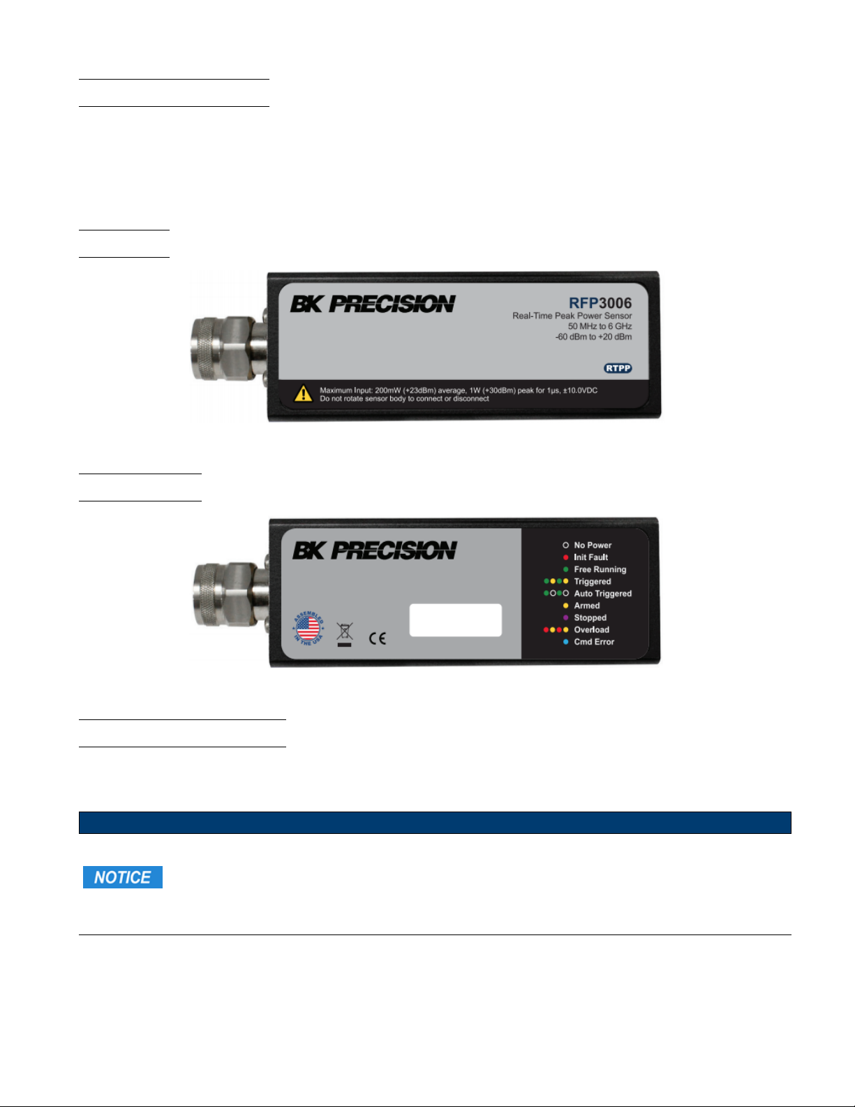
The information labels shown in gure 2.2 on the RF Power Sensor contain information on the maximum power levels
the device can handle.
The end panel, shown in gure 2.3, includes a Status LED. The color and ash pattern indicate the sensors status as
indicated on the label on the side panel shown.
Top View
Figure 2.2 Top View
Bottom View
Figure 2.3 Bottom View
2.3 Power Requirements
The RFP3000 Sensors require 2.5 Watts at 5 Volts, this is supplied via a USB port. The power sensor MUST be
connected to a USB 2.0 port that is able to supply the full 500 mA.
Note:
Usually a USB 2.0 port is capable of supplying 500 mA current through its port. When an unpowered
USB hub is used (sometimes the hub is internal), available current may need to be shared between
connected devices.
Page 15

Getting Started
This chapter will introduce the RFP Series RF Power Sensors, and will discuss basic connection and operation. For
additional information please see Chapter 4 "Operation".
3.1 Installing the Power Analyzer Software
This section describes the installation and use of the Power Analyzer Software for RFP Series RF Power Sensors. Before
you start, check your PC for software compatibility.
Note:
Do not connect the power sensor to your PC until you have installed the Power Analyzer Software.
The Power Analyzer Software requires the following minimum computer characteristics:
Processor
RAM
Operating System
Hard-Disk Free Space
Display Resolution
Interface
1.3 GHz or higher recommended
512 MB (1 GB or more recommended)
Microsoft® Windows® 10 (64-bit)
Min 1.0 GB free space to install or run
800x600 (1280x1024 or higher recommended)
USB 2.0 high speed
Procedure
To install the Power Analyzer Software, follow these steps:
1. Download the installation package from the Docs & Software tab of the product page on the BK Precision website.
2. The installation process is initiated by running “BPAInstaller.exe” with admin permissions.
• When you select install for the rst time, read the license agreement, accept it and then click on "Install" in order
to proceed with the installation process.
3. By default, the main software application will be installed in the following folder: C:\Program Files
(x86)\BKPrecision\Power Analyzer\.
– Once the installation has successfully completed, click the ”Close” button to exit the wizard.
4. Double click the Power Analyzer icon on the desktop to launch the application.
Page 16

Getting Started 16
3.2 Connecting the RFP Series RF Power Sensor
After unpacking and following the software installation discussed in chapter "Hardware Overview" and section Installing
the Power Analyzer Software, a sensor device can be connected to the USB port of the PC.
When the sensor device is rst connected to the USB port, there will be a one-time driver le installation. Wait until
Windows OS installs the driver le. An automatic device detection message will appear.
Note:
Older or newer operating system may behave dierently. Contact BK Precision if you have a problem.
The Windows pop-up shown in gure 3.1 noties that the USB driver for RFP3006 Sensor has been installed.
Figure 3.1 USB Driver Installed Notication
3.3 Introduction to the Power Analyzer Software
Upon installing the software, congured the USB drivers and connected the power sensor to the PC. The Power Analyzer
Software will be ready to take measurements.
Open the Power Analyzer Software from the BK Precision group in the Windows Start Menu or by double clicking
on the desktop icon .
A splash screen will welcome you to the application.
Figure 3.2 Power Analyzer Software Splash Screen
Page 17

Getting Started 17
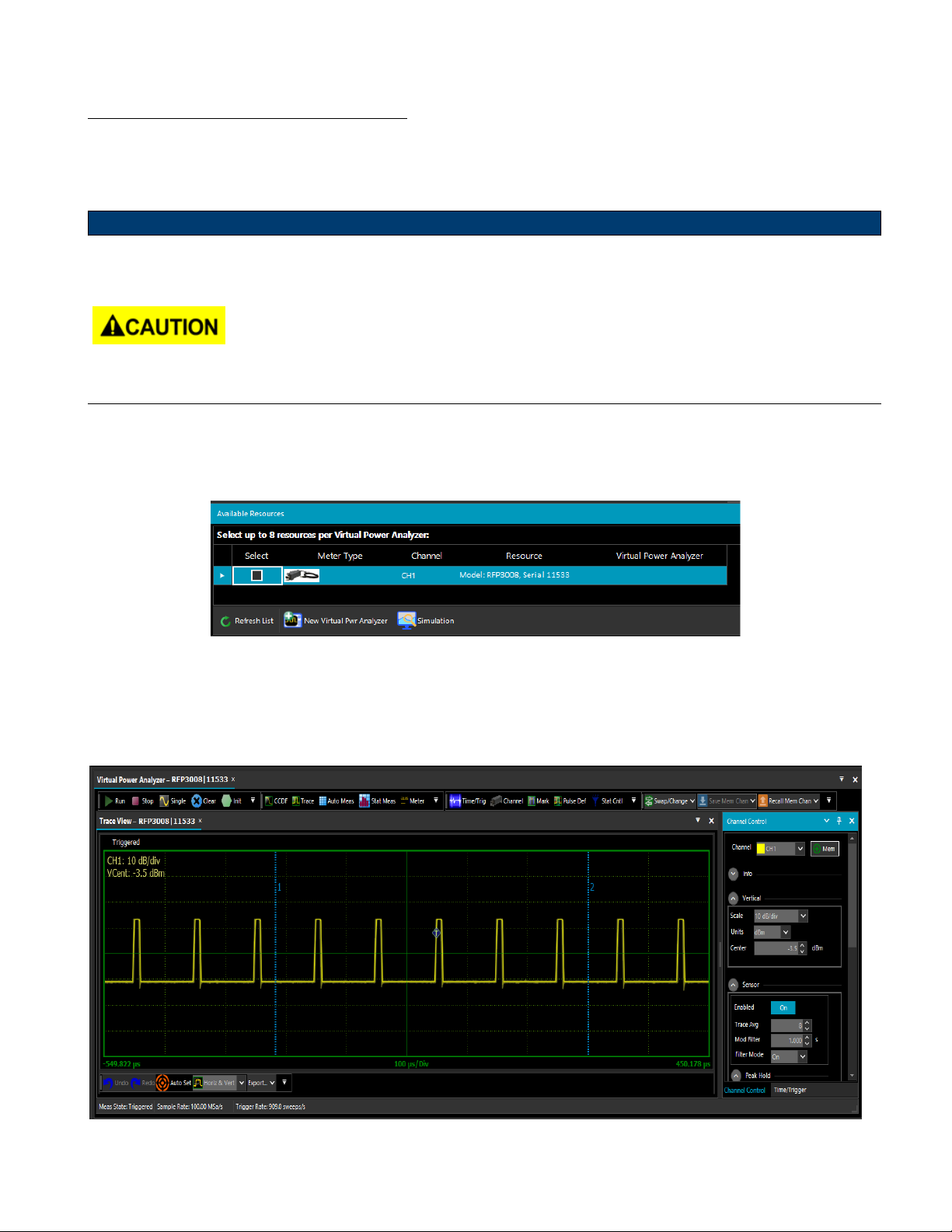
Under the "Available Resources Window", a pop up box will appear as below with the list of connected devices name
and hardware information. The initial view of the Power Analyzer Software is shown in gure 3.3. The display colors
may be dierent.
Figure 3.3 Available Resources
In the Available Resources window, check the “Select” box for one or more connected sensors, then click "New Virtual
Pwr Analyzer". This will launch a new Virtual Power Analyzer instance containing trace and control windows. If an RF
signal is connected to the USB sensor, the measured waveform will appear in the trace window.
A “Virtual Power Analyzer” is analogous to a benchtop RF Power Analyzer with one or more sensors connected. Time
and trigger controls are typically common to all sensors within a Virtual Power Analyzer, while channel-specic controls
are available for most other settings. This oers users the familiar, multi-channel approach common to power meters
and oscilloscopes.
When independent control of time base-related settings is desired, it is possible to open multiple Virtual Power Analyzers,
each with their own full set of controls.
Page 18

Getting Started 18
3.3.1 Docking Windows
The Power Analyzer Software uses dockable windows to allow the user to arrange the various windows in the cong-
uration of their choice. You can drag a docked window by clicking its title bar. This action enables you to move the
window to a dierent docked position or undock it.
To dock tool windows
• Click the tool window to dock.
• Drag the window toward the middle of the software main window.
• A guide diamond will appear with four arrows pointing toward the four sides of the main window.
• When the tool window being dragged reaches the location to dock it, move the pointer over the corresponding portion
of the guide diamond. The designated area is shaded blue.
• To dock the window in the position indicated, release the mouse button. Note that docked windows can be overlapped.
By selecting individual tab, it is possible to resize each tool windows and can be repositioned as below picture.
• A tool window can be docked to a portion of one of the side walls of the software by dragging it to the side until you
see a secondary guide diamond. Click one of the four arrows to dock the tool window to that portion of the side wall.
The following diagram shows the guide diamonds with arrows that appear when you drag a tool window toward the
center of the BK Precision software main window. The diamond on the right edge only appears when a tool window is
being dragged towards the edge of the main application window.
Figure 3.4 Docking a Sidebar
Note:
Each of the tool windows is highlighted as a rectangular box to be positioned by dragging in any direction within the
main window. Figure 3.4 is one example, but all the tool windows can be rearranged within the main software window.
Page 19

Getting Started 19
3.3.2 Main Application
The main application window is divided into several major sections and dockable windows depending on the type of
measurement selection. These windows can be arranged easily by docking and undocking within the main application
display area.
3.3.3 Available Resources Window
Sensors can be selected from the "Available Resources" window. A description for each connected resource will indicate
the hardware version, model and channel information including alias. User can select up to eight resources per Virtual
Power Analyzer. Following resource selection, click on "New Virtual Pwr Analyzer" and a new Virtual Power Analyzer
instance will open with a default conguration suitable for pulse measurements.
3.3.4 The Main Toolbox
Figure 3.5 Selecting a Sensor
Figure 3.6 Main Toolbar Controls
Page 20

Getting Started 20
3.3.5 Trace View Window
In order to display a pulse measurement, users must select the icon from the Main Toolbar.
The settings and settings related to pulse measurement can be selected from Main Toolbar and can
be applied to the measurement.
The Trace button on the Main Toolbar is used to setup and display a pulse measurement.
Figure 3.7 Main Toolbar
A measurement window conguration suitable for pulse measurements is shown in gure 3.8. This shows a large trace
window, automatic measurements, and a tabbed control box for time and channel settings.
Figure 3.8 Main Application Window
The Power Analyzer Software allows the user to directly enter numeric values for most settings in the Channel Control
and Time/Trigger windows. For many of the controls, additional methods such as increment/decrement or preset buttons
are available.
Page 21

Getting Started 21
Trace Pan and Zoom
The mouse can be used to select a zoom area to view detail in an area of interest on the displayed waveform. The
highlighted dragged rectangular area indicates the minimum area that will be shown when the zoom operation completes.
Horizontal pan or zoom adjusts the time base (within preset values) and the trigger delay to highlight an area of interest
without vertical rescaling.
Direct pan or zoom to waveform areas of interest is available by selecting any option from the lower toolbar of the trace
window. Available options for zoom/pan control are: Horizontal & Vertical, Horizontal, Pan and None with Undo and
Redo selections.
Figure 3.9 Zoom and Pan
Clicking on the Trace View display and dragging will open a zoom box, releasing the mouse button will result in the trace
being expanded to show the area contained in the zoom box
Auto Set
The button below the trace window attempts to congure level scaling, trigger level and timing for a “best t”
display based upon amplitude and timing of the applied signal. All other parameters are set back to defaults. If the Auto
Set process fails, all settings are left untouched.
Trace Data Export
Any trace window can be exported and saved or printed as a PDF or CSV document by selecting the button
from the lower toolbar of the trace window. An exported trace le can easily be imported into a spreadsheet or other
report le or documentation.
Page 22

Getting Started 22
3.3.6 Channel Control Window
Select the icon and a dockable sidebar will appear on the righthand
side of the main application window by default. This allows you to change all
related settings to control one or more sensor channels. Channel control setting
is dened by several parameters as listed below.
Channel: Select one or all channels (for multi-channels) via the dropdown list.
Selecting the "All" permits simultaneous update on all measurement channels
(up to 8) for most settings.
Units: Selects dBm, Watts or Volts measurement units. Selection aects
displayed text, measurements, and trace.
Vert Scale / Center: Sets vertical amplitude scaling and centering of the
displayed waveform. These settings aect only the trace display.
Sensor Enabled: Enable or disable individual connected sensors.
Trace Avg: Sets number of acquired sweeps averaged together for displayed
trace in pulse/triggered modes. Useful for noisy signals.
Mod Filter/Filter Mode: Sets manual or automatic lter integration time
window for measurements in modulated (non-triggered) acquisition modes.
Peak Hold Mode/Decay Count: Sets peak hold duration (# of sweeps).
Tracks Trace Avg setting or may be independent.
Video BW: Selects sensor video bandwidth, high or low.
Frequency: Sets measurement frequency for the applied RF signal.
Cal & Corrections: Oset compensates reading for external gain/loss.
Zeroing and Fixed Cal: Sensor zeroing and xed calibration can be performed
by selecting each specic button.
Figure 3.10 Channel Control Menu
Page 23

Getting Started 23
3.3.7 Time/Trigger Settings Window
Select the icon to customize all related settings for both time base and trigger of a pulse signal.
Time base: Acquisition time in seconds per division. The power sensors use a
xed grid of 10 divisions for the sweep extents. Settings are in a 1- 2-5
sequence. Consult series specications for time base range.
Trigger Delay: Trigger delay can be adjusted by manually entering a numerical
value into the eld or using the up-down arrow keys. Click the “0” icon to reset
the trigger delay to zero seconds (RTP5000 only).
Trigger Position: Trigger position can be changed by entering numerical values
into the “Divisions” eld, clicking the scroll arrows, dragging the slide control, or
by clicking the L/M/R (Left/Middle/Right) indicators.
Trigger Source: Several trigger modes are available for each trigger source
under "Trigger Control" section. Multiple trigger sources are available under the
drop-down list including both "Internal" and "External" selection.
Trigger Mode: Select Normal, Auto, Auto Level or Free run. Trigger Level:
Sets trigger level when trigger source is INT and trigger mode is Auto or
Normal.
Slope: Select rising or falling edge triggering.
Holdo: Sets trigger holdo time and selects between Normal or Gap holdo
mode.
Trigger Skew Adjustment: This feature allows the user to adjust the skew for
internal trigger with master trigger output, and also external and slave triggers.
Skew adjustments allow to calibrate out trigger delay between sensors so the
user can measure propagation delay of the DUT from input to output. Manual
skew adjustments can be made by entering the skew value in the numeric entry
eld. The button to the right of each skew adjustment is the Auto-Skew button
which is described in detail in section "Time/Trigger Control Window". This
feature allows automatic adjustment of the skew.
Figure 3.11 Time/Trigger Menu
Page 24

Getting Started 24
3.3.8 Marker Settings Window
Programmable markers can be moved to any portion of the trace
that is visible on the screen. They can be used to mark regions of
interest for detailed power analysis. The instrument can display
power at each marker, as well as average, minimum, and maximum
power in the region between the two markers.
Click the icon to control the settings for time markers and
amplitude reference lines of a pulse signal.
Markers: Time Marker position settings will allow you to change
both marker 1 and marker 2 time positions by using either arrow
keys or entering numerical values into the eld. It will also display
the time delta value between the two markers.
Reference Lines: Also known as Horizontal Markers, can be
enabled by selecting On/O button for each individual channel.
Once enabled, users may select several options for automatic
amplitude tracking from the Tracking drop down list: O,
Markers, TopBottom, DistalMesial and DistalProximal. Two
reference lines can be set by using up/down arrow keys. Horizontal
markers are useful to determine the dierence with regard to loss.
3.3.9 Pulse Denitions Windows
Click the icon to control the settings of the pulse
thresholds and the pulse gate.
Pulse Thresholds: Pulse denition setting allows user to dene
distal, mesial and proximal values for pulse thresholds. It is also
possible to change pulse unit from watts to volts.
Pulse Gate: Pulse start and end gate can be changed both
numerically and by changing up/down arrow keys.
Chapter 6 contains a detailed description of each pulse threshold
level and the pulse measurement process.
Figure 3.12 Marker Settings Menu
Figure 3.13 Pulse Denition Menu
Page 25

Getting Started 25
3.3.10 Automatic Measurements Windows
Select the icon to display a tabulated eld with a list of parameters for RF pulse measurements including marker
measurements. Below is an example screenshot for automatic parameters displayed for a typical pulse measurement.
Note:
All eld parameters are customizable, and can be edited or deleted from the list. The whole table can be copied and
pasted into a spreadsheet in order to make any custom report le along with captured screenshots by selecting export
button as provided by the software.
Automatic Pulse Measurements Automatic Marker Measurements Multiple Pulse Analysis
Figure 3.14 Auto Measurement
Page 26

Getting Started 26
Customize Field Parameters
All eld parameters under automatic measurement are
customizable, and can be edited or deleted from the list
by selecting individual parameter elds and then by using
right click button of the mouse.
Export or Copy Field Parameters
The whole automatic table or individual parameter eld can be
copied and then pasted into a simple spreadsheet or document
in order to make a custom report le along with captured
screenshots provided by the application.
To select multiple parameters right click using the mouse while
holding the Ctrl key.
Figure 3.15 Pulse Measurements Customize
Figure 3.16 Select Multiple parameters
Page 27

Getting Started 27
3.3.11 Display Settings Windows
The display settings allow for customization of data and trace colors for each measurement channel, and enable or disable
trace display features such as Average, Envelope, Maximum, Minimum and Persistence. It is also possible to adjust
marker color, background, grid colors and more under "Graph Colors" section of the display settings.
To open the Display Settings Windows left click on the Graph Settings icon located in the View tab.
Figure 3.17 Graph Settings
Figure 3.18 Display Settings
Page 28

Getting Started 28
3.3.12 CCDF View Window
For statistical measurements, select the icon from menu bar to view a CCDF graph. The sidebar on the CCDF
screen allows adjustment of horizontal scale, horizontal oset, cursor type, cursor position and dB oset. The user can
also enable/disable capture or reset the statistical data acquisition.
Figure 3.19 Complementary Cumulative Distribution Function Graph
3.3.13 Statistical Measurements Window
Select the icon, to tabulate a list of statistical measurements .
An example can be seen in gure 3.20
Figure 3.20
Statistical Measurements Window
Page 29

Operation
This section presents the procedures for operating the RFP Sensors using the Power Analyzer Software. All the display
windows that control the sensor are illustrated and accompanied by instructions for using each in the window.
4.1 Power Analyzer Software
The Power Analyzer Software is a Windows-based software program that provides immediate RF power measurements
from RFP Sensors without the need for programming on your Windows OS based computer. The measurements parameters from the power sensor can be displayed on your computer or can be integrated into a test system using an
Application Program Interface (API).
Note:
This section of the manual assumes that the Power Analyzer Software has been installed on a computer using the in-
structions provided in the "Getting Started" chapter of this manual.
4.1.1 Initializing the Software
Use a mouse or other pointing device to click on the View tab on the top of the window.
Click on Load Defaults – this will load the default Windows Theme ‘Visual Studio 2012 Dark’ and will reset all application
measurement settings to default values provide a known initial state.
Click on the down arrow adjacent to the theme to view the pull-down menu showing the available themes. The themes
establish the look of the Windows environment setting colors, fonts, and backgrounds.
The balance of this chapter will use the ‘Default” theme.
Click on any of the available themes to see what they look like. Select the theme you wish to use.
Figure 4.1 Selecting Theme
Page 30
Operation 30
4.1.2 Connecting the RFP Series Sensor
Connect the RFP Sensor to one of the USB ports of a computer using the supplied USB cable.
Connect power sensor to RF Source using the standard Type N connection port on the sensor.
Note:
• Do not turn the body of the sensor when connecting the sensor to a unit under test (UUT).
To avoid internal sensor damage, connect and disconnect the sensor by turning the metal
nut of the N connector only until it is ‘hand tight’.
• Ensure that you do not apply any excessive force on the sensor once it has been connected.
• Do not exceed the specied RF power at the RF input of the sensor.
Once the power sensor is connected, a pop up box will appear in the Power Analyzer Software as in gure 4.2 with
the list of connected devices name and hardware information.
Figure 4.2 Available Resources Window
Up to eight sensors can be connected to the software. Click on the “Select” box of one of the sensors, click the "New
Virtual Pwr Analyzer" button at the bottom, a new Virtual Power Analyzer window will show up. If you have an
RF signal connected already to the power sensor, the measured signal should display in the Trace View window which
appears along with the Channel Control tool window as shown in gure 4.3.
Figure 4.3 Trace View
Page 31
Operation 31
4.1.3 Trace View Display
The Trace View window in gure 4.3 displays a trace of power versus time. The readout in the upper left corner shows
the channel number of the trace, the vertical scale factor and the vertical center. In gure 4.3 Channel 1 is displayed
with a vertical scale of 10 dB/div(ision) and a vertical center of -3.5 dBm.
The horizontal scale of the trace in the Trace View window is shown at the bottom of the grid. At the center of the
horizontal axis is the horizontal scale factor. Numbers at the right and left ends of the horizontal axis show the trace
start and end times relative to the trigger.
The two vertical blue lines labeled 1 and 2 are markers used for measurements of the displayed signals. These will be
discussed later in the manual.
Trace View Toolbox
The bar at the bottom of the Trace View window provides a number of useful tools that can be used to optimize the
trace display and archive the trace(s):
• The Export menu box is used to export any trace window as a PDF or CSV document. These exported trace les
can be used for a report or document.
• The Undo and Redo buttons work in conjunction with the display expansion (zoom) function to
remove (Undo) and restore (Redo) changes in display scaling.
• Auto Set provides an automatic setup of the trace display scaling which optimizes the trace view in the Trace View
window.
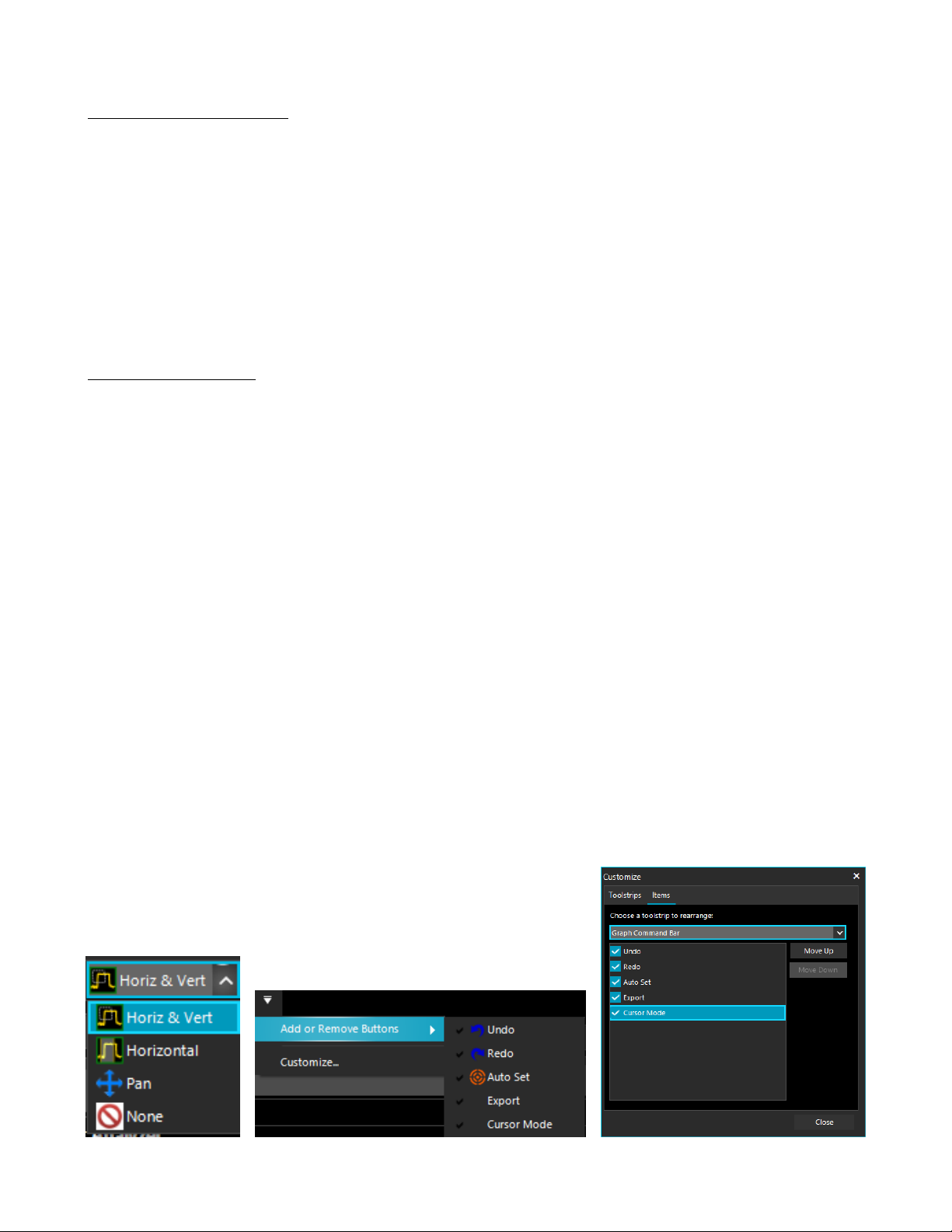
• The Cursor Mode menu box is used to select the zoom mode.
– Horiz(zontal) & Vert(ical) lets the graphical drag and drop zoom control both horizontal and vertical expansion.
– Horizontal limits the zoom controls to aecting the horizontal scaling only
– Pan allows the user to click and drag the trace either horizontally or vertically.
– None turns o both zoom and panning.
• The pull-down menu box is used to customize the Trace View toolbox.
– Add or Remove Buttons sets the tools to be displayed in the toolbox.
– Customize sets the order of the tools displayed in the toolbox.
Cursor Mode Add or Remove Buttons Customize
Figure 4.4 Trace View Toolbox Pull Down Menus
Page 32

Operation 32
Trace Pan and Zoom
The application has a trace zoom feature which lets a user to drag a rectangular box (like the one shown in gure 4.5)
around the trace in order to zoom onto a special area of the displayed waveform.
The highlighted dragged rectangular area indicates the minimum area that will be shown when the zoom operation
completes. The zoom area is constrained to the preset Time base settings and trigger Vernier limits.
Note that in gure 4.5 that the zoom horizontal scale changes from 10 µs/div to 50 ns/div the nearest available xed
Time base setting. Vertical scaling is similarly constrained.
Figure 4.5 Horizontal and Vertical Display Expansion
Note:
Horizontal or horizontal and vertical display expansion (zoom) is accomplished by clicking on the trace view and dragging
the mouse diagonally while holding the mouse button down. A box will outline the area to be expanded. Releasing the
mouse button will rescale the trace.
Page 33

Operation 33
4.1.4 Formatting Trace View Display
To open the Display Settings Windows left click on the Graph Settings icon lovated in the View tab.
Figure 4.6 Display Settings
The Display Settings pop-up is used to congure the Graph View. The elements to be displayed can be chosen and their
colors may be selected along with the background color.
The upper section of the Display Settings labeled Trace controls the conguration of the selected trace. There can be
a maximum of eight traces. The conguration of each trace includes the trace color, the choice of ve viewable trace
attributes, and the trace refresh time. Trace attributes include graphical view of the average value, envelope, maxima,
minima, and persistence (trace history). The defaults are to Show Avg and Show Envelope. Each of the selected elements
is overlaid on the trace.
Note:
The sensor acquires all three "traces" (average, min and max) when required . These are used for several of the marker
measurements such as interval peak-to-average, and others.
For the marker intervals, Min and Max (highest maximum trace and lowest minimum trace points) as well as MinF and
MaxF (min and max ltered) which are the highest and lowest points on the average trace.
The former measurements are useful for looking at modulation, while the latter are most useful for seeing systematic
peaks and dips (for example, ringing) of a repetitive waveform with the noise reduced.
A check box for Disable HW Acceleration can be checked if the computer does not have a monitor or graphics card or
if it is being operated remotely using remote desktop. Note: This change will not take eect until the next time a trace
window is opened.
The lower section of the Display Settings pop-up provides controls for color choices for trace grid, border, and background.
Markers, axis label, crosshair color selections are also included. Color choices are made by clicking on the ellipsis symbol
(…) adjacent to each element. This will bring up the Color Dialog palette used to set the desired color for the element.
Page 34

Operation 34
4.1.5 Main Toolbar
The Power Analyzer Software always displays the Main Toolbar that is located at the top of the main program window
and contains shortcuts to commonly used functions and measurements.
The Main Toolbar can be customized as discussed below. Figure 4.7 shows the Main Toolbar:
Figure 4.7 Main Toolbar
The Main Toolbar contains three sections called Toolstrips. The group of shortcuts on the left, including CCDF, Trace,
Auto Meas(urement) and Stat(istical) Meas(urement) are the Measurement Windows Toolstrip and will bring up
trace display or measurement windows. The middle group with Time/Trig, Channel, Mark, Pulse Def(initions) and
Stat(istical) Cntl(Control) are the Control Windows Toolstrip, and will cause setup and control windows to be displayed.
The nal group including Run, Stop, Single, Clear and Init(ialize) are the Acquisition Control Toolstrip and aect the
state of the acquisition.
Any of the toolstrips may be separated from the Main Toolbar and re-positioned by clicking on the ellipsis symbol at the
left end of any of the groups and dragging the toolstrip.
The drop-down menu bar on the right of each section allows the user to edit the tools bar by adding or removing any of
the items under the Items tab. The Toolstrips tab allows the user to show or hide the tools strips.
Acquisition Control Toolstrip
Figure 4.8 Acquisition Control Toolstrip
The buttons on this toolstrip control the state of the acquisition:
• Run – Starts the measurement acquisition and allows it to run continuously until stopped.
• Stop – Stops the measurement acquisition.
• Single – Starts a single measurement acquisition and then stops.
• Clear – Erases the acquired data trace. Useful in clearing a single or averaged acquisition.
• Init – Initializes or resets all settings for the active Virtual Power Meter to default values.
Page 35

Operation 35
Measurement Control Toolstrip
Figure 4.9 Measurement Control Toolstrip
The buttons on this toolstrip create Trace View and CCDF Graph displays as well as the automated power measurement
and statistical Measurement tabular display windows:
• CCDF – This button turns on the complementary cumulative distribution function (CCDF) display. If the CCDF
display is already opened but hidden behind the Trace View display this button will bring the CCDF trace to the
foreground.
• Trace - This button turns on the Trace View trace that displays power versus time.
• Auto Meas – This button opens Automatic Measurement windows showing the automatic Pulse and Marker Measurements tables.
• Stat Meas – This button opens the Statistical Measurements window displaying the measurements associated with
the CCDF Graph.
Control Windows Toolstrip
Figure 4.10 Control Windows Toolstrip
The buttons on this toolstrip control the setup windows for the acquisition, and measurement functions.
• Time/Trig – This button displays the Trigger and Time base control windows.
• Channel – This button brings up the Channel Control Window allowing control of the vertical range and oset as
well as sensor related settings
• Mark – This button causes the Marker Settings window to be displayed. Marker and reference lines can be controlled
from here.
• Pulse Def – This button displays the Pulse Denitions window controlling the pulse measurement thresholds, units,
and gating.
• Stat Cntl – This button brings up the Stat(istics) Mode Control window with scaling and population control for the
CCDF display.
Page 36

Operation 36
Memory Channel Toolstrip
Figure 4.11 Memory Channel Toolstrip
The Memory Channel toolstrip contains Swap/Change, Save Mem(ory) Chan(nel), and Upload Mem(ory) Chan(nel), and
controls the sensor connection source and saving and recalling Mem(ory) traces. The Memory Channel is a reference
trace that appears on the Trace View when Mem+ is enabled.
• Swap/Change - Swap/change allows you to change sensors for a particular session if more than one is connected.
• Save Mem(ory) Chan(nel) – Saves the current Memory channel to a user selected folder on the computer.
• Upload Mem(ory) Chan(nel) – recalls a stored Memory Channel to the Memory Channel Trace on the Trace View.
Page 37

Operation 37
4.1.6 Time/Trigger Control Window
Pressing the Time/Trig button icon the Control Windows toolstrip will bring
up the Time base / Trigger Control window shown in gure 4.12
This window has four sections Time(base), Trigger Position, Trigger Con-
trol, and Trigger Skew Adj(ust). Any of these sections can be opened or
collapsed by clicking on the up/down arrow buttons to the left of the section
titles.
Time and Trigger Position Controls
Settings in the Time and Trigger Position Control groups aect horizontal
scaling and position of the acquired waveform.
Time base controls the Time base or horizontal scale of the acquisition and
is noted on the horizontal axis label of the Trace View. The Time base pulldown menu permits selection of xed Time base ranges from 5 ns/div to 50
ms/div (sensor series dependent) in a 1-2-5 progression.
Trig(ger) Delay can be adjusted either manually entering a numerical value
into the eld or using the up-down arrow keys.
The trigger delay time is set in seconds with respect to the trigger. Positive values mean that the trace display shows a time interval after the trigger
event. This positions the trigger event to the left of the trigger point on the
display, and is useful for viewing events during a pulse, or some xed delay
time after the rising edge trigger. Negative trigger delay mean that the trace
display shows a time interval before the trigger event, and is useful for looking at events preceding the trigger edge.
Pressing the ‘0’ button to the right of the trigger delay entry eld resets the
trigger delay to zero.
The range of trigger delay times is dependent on the Time base setting and
is summarized in table 4.1. Note the range will also depend upon the trigger
position.
Time base Setting Trigger Delay Range
5 ns/div to 10 us/div -1.26 ms to 100 ms
20 us/div -1.26 ms to 200 ms
50 us/ div -5.04 ms to 200 ms
100 us/ div -6.3 ms to 500 ms
200 us/div -12.6 ms to 1
500 us/div -31.5 ms to 1 s
1 ms/div -63 ms to 1 s
2 ms/div to 10 ms/div -126 ms to 1 s
20 ms/div -252 ms to 1 s
50 ms/div -628 ms to 1 s
Figure 4.12
Time/Trig Control Window
Table 4.1 Trigger Delay Range
Page 38

Operation 38
Note:
Trigger delay ranges in table 4.1 are for the trigger position set to 0 divisions (Left). If trigger delay and position settings result in a pre-trigger capture interval greater than 1.26 ms, the sensor will automatically reduce the sample rate to
avoid overowing its pre-trigger memory.
Trigger Position controls are used to set the location of the trigger point on the acquired trace waveform. It can be
changed by entering numerical values into the Divisions eld from -30 to +30 divisions, by positioning the horizontal
slider bar, or by clicking on the L, M or R indicators to select one of three default positions: Left (zero divisions), Middle
(ve divisions) or Right (ten divisions).
Trigger Controls
Settings in the Trigger Control group provides control to aect the trigger source, mode, trigger level, slope, and trigger
holdo.
Trigger Source
The trigger source can be any of the resource channels (CH1, CH2, etc.), or the Ext(ernal) trigger input signal. The
Ind(ependent) trigger setting allows each connected sensor to trigger independently from its own RF input.
The external trigger is attached to the RTP Series Real-Time Power Sensors via the Multi-I/O connector adjacent to the
USB port on the RTP Series Real-Time Power Sensors. The connector is an SMB type. The external trigger requires a
TTL signal level, minimum pulse width of 10 ns, and maximum frequency of 50 MHz.
In a multichannel set-up, the sensors can be triggered independently as described above or in a master/slave conguration.
In master/slave conguration, one channel (CH1, CH2, etc.) is selected as the source (master) and the remaining sensors
automatically operate in slave mode. See Multichannel Operation for additional information.
Trigger Mode
There are four available trigger modes: Normal, Auto, Autolevel, and Freerun.
• Normal – The unit triggers when the amplitude of selected trigger source transitions above the preset trigger level
when positive trigger slope is selected or if it transitions below the preset trigger level when negative trigger slope is
selected. No automatic trigger actions takes place.
• Auto- Auto trigger mode operates in much the same way as Normal trigger mode, but will automatically generate
a trace if no trigger edges are detected for a period of time. If a triggerable signal edge occurs during auto-trigger
operation, the trigger system will resynchronize with the signal. For trigger rates below approximately 10 Hz, the
Auto trigger time delay may interfere with resynchronization. Use Normal mode if this occurs.
• AutoLevel - performs the same function as Auto and, in addition, automatically sets the trigger level based on the
peak-to-peak amplitude of the signal. For many signals this will provide a fully automatic trigger system. For slow
rate signals and complex level patterns, it may not produce the desired display. Use Normal mode if this occurs.
• Freerun - Free Run generates horizontal sweeps asynchronously, without regard to trigger conditions. This mode is
useful for locating low duty-cycle events visually.
Trigger Level
Sets the threshold level for the trigger signal in the Auto and Normal trigger modes. The trigger level can be entered
numerically or changed by using arrow keys. The trigger level range has a maximum value of 20 dBm and a minimum
range that is sensor model dependent (see the sensor specications for your specic sensor model)
Page 39

Operation 39
The trigger range is automatically adjusted to include the dB Oset parameter selected in the Cal & Corrections section
of the Channel Control window. For example, if the trigger level = 10 dBm and the dB Oset is changed from 0 to 20
dB, then the oset-adjusted trigger level will be displayed to the user as 30 dBm. Likewise, the maximum trigger level
range will be extended to 40 dBm. The trigger level set point and setting range are both shifted upward by 20 dB.
Trigger Slope
Sets the trigger slope or polarity. When set to Pos(itive), trigger events will be generated when a signal’s rising edge
crosses the trigger level threshold. When Neg(ative) is selected, trigger events are generated when the falling edge of the
pulse crosses the threshold. Trigger slope can be selected by using Pos and Neg button boxes under slope.
Holdo (Time)
The holdo time can be entered and adjusted numerically to 0.01 µs resolution, or using the up and down arrow keys in
1 µs increments. The eect of Holdo time depends on the Holdo Mode. Set the trigger holdo time in microseconds.
Holdo Mode
There are two trigger holdo modes: Normal and Gap.
Normal Holdo
Normal trigger holdo is used to disable the trigger for a specied amount of time after each trigger event.
The holdo time starts immediately after each valid trigger edge, and will not permit any new triggers until
the time has expired. When the holdo time is up, the trigger re-arms, and the next valid trigger event
(edge) will cause a new sweep. This feature is used to help synchronize the RTP Series Real-Time Power
Sensors with burst waveforms such as a TDMA or GSM frame. For periodic burst signals, the trigger
holdo time should be set slightly shorter than the burst or frame repetition interval.
Gap Holdo
Gap or frame holdo is very useful for packet-based communication signals where the transmission burst
contains deep modulation which may fall briey below the trigger threshold, or when bursts or pulses are
of varying length and spacing, making normal holdo ineective. In most cases, the "o" time between
transmission bursts, or frames, is considerably longer than the instantaneous modulation dips.
In gap holdo the trigger is not armed until the trigger source remains inactive (below the trigger threshold
for positive trigger slope, or vice versa for negative slope) for at least the set duration. If trigger polarity
is positive, and gap holdo is set for 1 us, then the signal must stay below the trigger level for at least 1 us
before the trigger is armed. Then, the next rising edge following a gap of 1 us or longer will trigger the
acquisition.
Page 40

Operation 40
Trigger Skew Adj(ust)
Trigger Skew aligns the edge crossing with the trigger point for each of the trigger sources. This is done internally by
adding a trim value to the trigger delay setting. Since the dierent trigger sources (internal, external, and slave) have
dierent delays, the system stores a value for each.
Trigger Skew requires a fast RF pulse (Trise < 10 ns) to adjust ’Int’ skew. To auto-adjust ’Ext’ requires a fast RF pulse
aligned with a fast external trigger pulse applied to the sensor’s MIO input. Adjusting the ’Slave’ source requires two
sensors connected to a common, fast RF pulse (Trise < 10 ns) and interconnected for cross-trigger via their MIO inputs.
You can de-skew one setting at a time until all three sources are calibrated.
Deskewing can be done automatically by clicking on the double slope icon on the left of “ns”, shown in gure ??
Automatic deskewing requires a fast edge, repetitive signal.
Figure 4.13 Trigger Skew Adj
Page 41

Operation 41
4.1.7 Channel Control Window
The Channel Control window allows you to change all related settings to
control sensor channels. The Power Analyzer Software has the capabil-
ity of handling multiple control channels by selecting each individually from
the drop-down list. Channel control setting is dened by several parameters
as listed below:
Channel
You can select an individual channel or all measurement channels (for
multichannel operation) by using the drop-down list. The channel labeled
MEM1 is a memory channel which is a reference trace that can be stored
or recalled as need.
The button causes the current trace to be stored in the Memory
Channel. The current memory channel can be stored to the computer hard
drive using the Save Mem Chan button in the Memory channel toolstrip.
Likewise, a previously stored memory trace can be recalled using the
Upload Mem Chan button.
To turn o the Memory Channel, select MEM1 or MEM2 from the Channel
drop down menu, then click on the “On” button next to "Enabled" in the
Sensor menu (see below) to select “O”.
Info
The Info group shows the pertinent information for the selected sensor.
Sensor model number,serial number, and rmware and FPGA versions for
the selected channel are displayed in this group.
Pressing the Advanced button will result in a Sensor Info pop-up with
three tabs: Sensor Data, Cal Factors, and Hardware Info.
Sensor Data contains identication and calibration information
for the sensor.
Cal Factors contain the frequency response calibrations factors
for both high and low bandwidth calibration.
Hardware Info contains information on the current state of the
sensor hardware including the detector temperature and key power
source voltage readings.
Figure 4.14 Channel Control Window
Page 42

Operation 42
Vertical
The Vertical group contains controls that aect vertical settings for the selected power sensor.
Scale - Vertical scale sets the scaling of the level axis of the Trace View based on the selection of units as shown in table
4.2
Units Scale
dBm 0.1, 0.2, 0.5 1, 2, 5, 10, 20, 50 dB/div
Watts 1 pW to 500 MW/div in a 1-2-5 progression
Volts 1 µV to 100 kV/ div in a 1-2-5 progression
Table 4.2 Vertical Scale Range
Units - The trace presentation may be shown in units of dBm, Watts or Volts. The Units selection determines the range
of the scale values. Note that the Units setting also aects text measurement values in the Measurement windows.
Center - Set the power or voltage level of the horizontal centerline of the graph for the specied channel in the selected
channel units. The center position can be entered numerically or adjusted by using up and down arrow keys.
Sensor
The Sensor group controls acquisition parameters for the selected power sensor.
Enabled - Individual sensors or all the selected sensors can be enabled or disabled by using the alternate action On/O
button. This functionality also enables or disables the MEM channels.
Trace Avg – Trace averaging can be used to reduce display noise on both the visible trace, and on automatic marker
and pulse measurements. Trace averaging is a continuous process in which the measurement points from each sweep are
weighted (multiplied) by an appropriate factor and averaged into the existing trace data points. In this way, the most
recent data will always have the greatest eect upon the trace waveform, and older measurements will be decayed at a
rate determined by the averaging setting and trigger rate. This averaging technique is often referred to as ‘exponential’
averaging because averaging imposes a rst-order Innite Impulse Response (IIR) exponential lter with a time constant
of "n" where n is the Trace Avg (number of averages) setting.
Sensor averaging can be set by selecting a number of averages from 1 (no averaging) to 16384 in binary steps using the
up and down arrow buttons in the Trace Avg eld.
Note:
For Time base settings of 200 ns/div and faster, the sensor acquires samples using a technique called equivalent time or
random interleaved sampling (RIS). In this mode, not every pixel on the trace gets updated on each sweep, and the total
number of sweeps needed to satisfy the average setting will be increased by the sample interleave ratio of that particular
Time base. At all times the average trace is the average of all samples for each pixel, and the min/max are the lowest
and highest of that same block of samples for each pixel.
Page 43

Operation 43
Mod Filter sets the modulation lter integration time. It is used in modulated mode measurements and does not aect
the pulse mode (triggered) measurements shown in the trace view. The modulation lter is a “sliding window” lter
which averages samples taken within a time window whose duration is set by this eld. All samples within the time
window are equally weighted.
Filter Mode controls the modulation lter. The lter can be set to On (manual lter time setting), None (integration
time is set to the minimum 1 ms value), or Auto (integration time automatically selected based upon input level).
Peak Hold settings control the operating mode of the selected channel’s peak hold function. Peak Hold aects the
envelope trace (if displayed) as well as peak or dynamic range marker and pulse measurements.
In Tracking mode, the maxima and minima traces "decay" towards the average with a time constant that is
the same as the averaging setting. If averaging is set fast (Trace Avg is set to a low value), then the maxima
and minima decay quickly (are not held very long) while long averaging (Trace Avg is set to a high value) settings yields a ‘atter’ trace and maxima and minima peaks decay slowly back to the average power level.
In Manual mode the averaging and peak time constants are independent (do not track each other). Rather,
peaks are held for a time proportional to the Decay Count setting. Decay Count can be set from 1 to 16384
and increments in binary steps.
Manual mode can be useful if you want to set averaging short to see short-term signal uctuations from one
trace to the next, yet want the peaks held for a long time to get a better feel of longer-term peak stress on
your system.
The Innite Hold button sets the Decay Count to innity. Signal peaks and dips are held indenitely and
never decayed. This is useful for long-term monitoring for glitches, spikes, dropouts, or other intermittent signal events.
Note:
The eects of the peak hold, i.e. min/max decay, are only visible when the "envelope" or "min/max" display is
enabled in the view options (See section 3.3.11 and the associated gure 3.18. The marker min/max values
are always aected.
Video BW sets the sensor video bandwidth for the selected sensor. High is appropriate for most measurements, and the
actual bandwidth depends upon the sensor model. Low bandwidth oers additional noise reduction for CW or signals
with very low modulation bandwidth. If Low bandwidth is used on signals with fast modulation, measurement errors may
result if the sensor cannot track the fast-changing envelope of the signal.
Frequency should be set to the RF frequency that is applied to the sensor for the current measurement. The appropriate
frequency calibration factor from the sensor’s calibration table will be interpolated and applied automatically. Application
of this calibration factor compensates for the eect of variations in the atness of the sensor’s frequency response.
The power sensor has no way to determine the carrier frequency of the applied signal, so the user must always enter the
frequency.
Page 44
Operation 44
Cal & Corrections
The Calibration and Corrections group controls coarse and ne corrections to the measurements.
Oset - Sets a measurement oset in dB for the selected sensor. This is used to compensate for external
couplers, attenuators or ampliers in the RF signal path ahead of the power sensor.
Zero - Performs a zero oset null adjustment. The sensor does not need to be connected to any calibrator
for zeroing. This action removes the eect of small, residual power osets, and should be performed prior to
low-level measurements. Note that there should be no RF signal applied to the sensor input prior to zeroing.
Fixed Cal - Performs a calibration at 0 dBm at the currently set frequency. This requires a calibrated 0 dBm
(1.00 mW) signal source at the current measurement frequency.
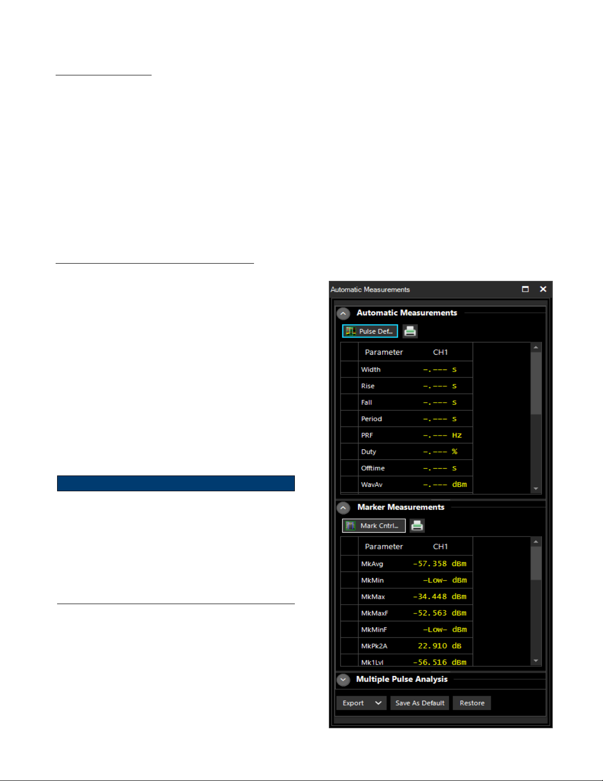
4.1.8 Automatic Measurements Display
Clicking on the AutoMeas icon in the Measurement
Control Toolstrip will bring up the Automatic Measurements window to the left of the Trace View as shown
in gure 4.15. This window includes two related subwindows, Pulse Measurements and Marker Measurements. The Pulse Measurements window shows the
sixteen default eld pulse parameters. The eld pulse
parameter measurements are computed with methods
described in IEEE Std 181™-2011 and detailed in Section 6 on pulse terms and denitions.
The Marker Measurements window shows twenty-one
marker measurements.
Note:
All eld parameters are customizable, can be edited or
deleted from the list by selecting individual parameter
elds and then by using right click button of the mouse.
The whole table can be copied and pasted into a spreadsheet in order to make any custom report le along with
captured screenshots by selecting export button as provided by the software.
Figure 4.15 Automatic Measurements Window
Page 45

Operation 45
Any individual parameter or group of parameters on pulse or marker measurements can be highlighted by left clicking
with the mouse and using the up and down arrow keys a group of them can be selected. Selected cells can be copied
by right clicking on the parameter(s) and selecting copy. The copied cells can be pasted into a spreadsheet or document.
Clicking on the printer icon next to either table will open a Print Preview window allowing the user to print the table.
Clicking on the Export button will open a viewer showing the whole table. The contents of the viewer can be saved or
printed as PDF or CSV les, if desired.
4.1.9 Pulse Denition Window
Clicking on the Pulse Def button in the Pulse Measurement title bar or on
the Pulse Meas button on the Measurement Control Toolstrip will open
the Pulse Denitions window shown in Figure 4.11. This window contains
the pulse thresholds, pulse analysis units and gate settings for the selected
sensor.
Pulse Thresholds
Pulse denition settings allows user to dene distal, mesial, and proximal
values for pulse thresholds, and the pulse units.
Distal - Sets the pulse amplitude percentage that denes the end
of a rising edge or beginning of a falling edge transition. Typically,
this is 90% voltage or 81% power relative to the top level of the
pulse. This setting is used when making automatic pulse risetime
and falltime calculations.
Mesial – Sets the pulse amplitude percentage that denes the
midpoint of a rising or falling edge transition. Typically, this is 50%
voltage or 25% power relative to the top level of the pulse. This
setting is used when making automatic pulse width and duty cycle
calculations.
Proximal – Sets the pulse amplitude percentage that denes the
beginning of a rising edge or end of a falling edge transition.
Typically, this is 10% voltage or 1% power relative to the top level
of the pulse. This setting is used when making automatic pulse
risetime and falltime calculations.
Pulse Units – Controls whether the distal, mesial, and proximal thresholds are computed as voltage or power
percentages of the top/bottom amplitudes. If Volts is selected, the pulse transition thresholds are computed as
voltage percentages, and if Watts, they are computed as power percentages.
Figure 4.16 Pulse Denition Window
Many pulse measurements call for 10% to 90% voltage (which equates to 1% to 81% power) for risetime and
falltime measurements, and measure pulse widths from the half-power (–3 dB, 50% power, or 71% voltage)
points. The Pulse Units setting is independent of the channel’s display units setting.
Page 46

Operation 46
Pulse Gate
The Pulse Gate settings dene the measurement interval for the following power related pulse measurements: Pulse
Average, Pulse Peak, Pulse Minimum and Pulse Droop/Tilt. Pulse timing measurements between mesial crossings such
as width and period are not aected. The purpose of the Pulse Gate setting is to exclude edge transition eects from
the pulse power measurements. Automatic pulse measurements are then performed between Start Gate and End Gate
points.
Start Gate - Sets the beginning of the pulse measurement region as a percentage of the pulse width. The Start Gate
has a continuous range of 0.0 % to 40.0 % of the pulse width and may be entered numerically or varied using the up or
down arrows.
End Gate - Sets the end of the pulse measurement region as a percentage of the pulse width. The End Gate has a
continuous range of 60.0 % to 100.0 % of the pulse width and may be entered numerically or varied using the up or
down arrows.
4.1.10 Marker Settings Windows
Clicking on the Mark Ctrl button in the Marker Measurement title bar or
on the Mark button on the Measurement Control Toolstrip will open the
Marker Settings window shown in gure 4.17. This window contains vertical
marker locations, marker delta, and horizontal reference line locations for the
selected sensor.
Markers
Time Markers are a pair of vertical cursors that allow level measurements
at specic times relative to the trigger event. Markers can be moved to any
portion of the trace that is visible on the screen, and these can be used to
identify regions of interest for detailed power analysis. Power measurements
can be performed at each marker, as well as average, minimum and maximum power in the time interval between the two markers.
Marker 1 and Marker 2
Marker settings will allow you to change both marker 1 and marker 2 positions by using either arrow keys or entering numerical values into the eld.
The Marker locations can also be set graphically by clicking on the marker in
the Trace View and dragging the marker left or right.
Marker Delta
The Marker Delta window indicates the time interval between Marker 1 and
Marker 2.
Figure 4.17 Marker Settings Window
Page 47

Operation 47
Reference Lines
The reference lines, Reine 1 and Reine 2, are horizontal lines displayed on the Trace View. They can be used to indicate
set amplitude levels for each sensor, or measurement-specic levels.
Channel
Selects the channel that the reference lines will be applied to.
Enabled
Turns the reference lines on or o for the selected channels. When o, reference lines are not visible.
Tracking
The Reference Line Tracking setting allows the selection of either manual control of the reference line amplitudes or
selection of a set of commonly used reference amplitudes.
O – Allows the reference levels to be set independently using the Reine 1 and Reine 2 entry elds. Levels
can be entered numerically or by using the up and down arrows. The reference levels can also be set graphically by clicking on the reference line in the Trace View and dragging the line up or down. The vertical units
match the Units selection in the Channel Control window.
Markers – Links the reference levels to the amplitudes where the markers cross the pulse waveform on the
Trace View. Reference level Reine 1 will track the amplitude where Marker 1 crosses the pulse waveform and
Reine 2 will track the amplitude where Marker 2 crosses the pulse waveform.
TopBottom – Moves Reine1 to the measured Top amplitude and Reine 2 to the measured Bottom amplitude.
DistalMesial - Moves Reine 1 to the measured distal (upper pulse threshold) amplitude and Reine 2 to the
measured mesial (mid pulse threshold) amplitude. Pulse threshold levels are those set in the Pulse Denitions
window.
DistalProximal - Moves Reine 1 to the measured distal (upper pulse threshold) amplitude and Reine 2 to
the measured proximal (lower pulse threshold) amplitude. Pulse threshold levels are those set in the Pulse Definitions window.
Figure 4.18 Tracking
Page 48

Operation 48
4.1.11 Statistical CCDF Graph Display
The statistical analysis of the current sample population is displayed using a normalized Complementary Cumulative
Distribution Function (CCDF) presentation shown in Figure 4.13. The CCDF expresses the probability of occurrence of
a range of peak-to-average power ratios on a log-log scale, and a cursor (green diamond) allows measurement of power
or percentage at a user-dened point on the CCDF. As with all other graphical displays, the trace can be easily scaled
and zoomed, or the statistical data may be presented in a tabular format.
Figure 4.19 CCDF Graph
The CCDF has become a useful tool for analyzing communication signals that have a Gaussian like distribution (CDMA,
OFDM) where signal compression can be observed at rarely occurring peaks. It is most often presented graphically using
a log-log format where the X axis represents the relative oset in dB from the average power level and the log-scaled Y
axis is the percent probability that power will exceed the X-axis value.
At the bottom of the CCDF Graph window is a status bar reporting Stat Capturing status (On or O), Gating type
(Markers or Freerun), Total Time (HH:MM:SS) and the number of Points (Mega Samples) in the statistical population.
Additionally, there is an Export button and a Show Gaussian Ref check box. Clicking on the Export button will bring
up a Viewer pop-up window oering the ability to export the CCDF Graph in PDF or CSV format. Actuating the Show
Gaussian Ref displays a Gaussian CCDF reference curve on the graph, as shown in gure 4.19.
Page 49

Operation 49
4.1.12 Statistical Mode Control Window
The Stat Mode Control window, shown in gure 4.20, will appear when the CCDF Graph is displayed or by pressing
the Stat Ctrl button on the Control Windows toolstrip. The Stat Mode Control window controls the data acquisition
for the CCDF Graph.
Capture – Select “On” to begin acquiring samples. “O” stops the
acquisition.
Reset – Clicking on Reset clears the acquired statistical sample population.
If Capture is ON, a new acquisition will begin.
Term Action – Selects the action to take when either the terminal count
is reached or the terminal time has elapsed. The available choices are Stop,
Restart, or Decimate.
Stop - Stop accumulating samples and hold the result.
Restart - Clears the statistical sample population starts a new one.
Decimate - Divide all sample bins by 2 and continue. The total
sample count will be halved each time decimation occurs. This
should have very little visible eect on the CCDF values, since the
entire population is decimated uniformly and the shape of the
distribution is maintained.
Term Count – Sets the terminal sample count for the CCDF acquisition.
The range of values is 0.1 to 1,000,000 mega samples.
Terminal Time – Terminal Time sets the terminal running time for the
CCDF acquisition. The range of values is 1 to 3600 seconds.
Figure 4.20 Stat Mode Control
Horiz Oset – Horiz(ontal) Oset sets the horizontal oset for the CCDF
Graph statistical display. The value in dBr chosen will appear at the leftmost
edge of the graph. The range of values is -50.00 dBr to +50.00 dBr.
Horiz Scale - Selects the horizontal scale for CCDF Graph statistical display. Scale factors are from 0.1 to 5 dB/div
in a 1-2-5 progression.
Cursor Type - Select the independent variable for the CCDF cursor. If Percent is selected, relative power at the cursor’s intersection with the CCDF curve will be measured. If Power is selected, probability at the cursor’s intersection
with the CCDF curve will be measured.
Cursor Pos – Sets the CCDF cursor to the desired probability or power depending on the setting of Cursor Type.
Gating – Selects Marker or Freerun gating for statistical acquisition. If Markers are selected, then only samples
within the time marker interval on the Pulse Mode triggered sweep will be included in the statistical sample population. If Freerun is selected, then all the samples are acquired without regard to sweep acquisition.
Mark Ctrl – Clicking on this button will bring up the Marker Settings window allowing Marker locations to be set
easily when marker gating is used for statistical capture.
Page 50

Operation 50
Statistical Measurements Display
Clicking on the Stat Meas icon on the Measurement Control toolstrip brings up the Statistical Measurements window
shown in gure 3.20. This display of tabulated eld parameters is displayed on the left side of the CCDF Graph by
default.
These key statistical parameters are described in table 4.3.
Parameter Measurement Description
10% to 0.0001%
Pct at 0 dB Displays %CCDF at the average power.
Cursor Pct Displays %CCDF at the stat mode cursor.
Cursor Pwr
Average
Max Displays absolute maximum power.
Min Displays absolute minimum power.
Peak/Avg Displays crest factor (pk/avg ratio).
Dynamic Rng Displays dynamic range (max/min ratio).
Displays crest factor relative to population average
power at each specied %CCDF.
Displays crest factor relative to population average
power at the Stat Mode cursor.
Displays absolute average power of the statistical sample
population.
Table 4.3 Statistical Parameters
At the bottom of the Statistical Measurements window status is reported by
four elds: Stat Capturing status (On or O), Gating (Markers or Freerun),
Total Time (HH:MM:SS), and number of Points (Mega samples) in the statistics. Additionally, there is an Export PDF button. Clicking on the Export
PDF button will bring up a PDF Viewer pop-up window oering the ability
to export the CCDF Graph in PDF format.
Figure 4.21 Statistical Measurements
Page 51

Operation 51
4.1.13 Meter View
Meter view uses Modulated Measure Mode which is designed for continuous, true average power measurements of complex
modulated signals. The mode is similar to the operation of a conventional CW power meter, but does not suer the
measurement inaccuracies that occur when some diode sensors are used to measure modulated signals.
Modulated measurement mode is a continuous measurement mode primarily for continuously modulated or CW signals.
Continuous (untriggered / free run) sample acquisition is performed using “sliding window” ltering on the samples.
Filtered average power, peak power and minimum power measurements are continuously performed. The measured result
is the average power of the signal. Since the graphic display would basically just show a straight line, measurements in
this mode are best viewed using the Modulated Measurements display window. Figure 4.22 shows a Modulated Mode
measurement displaying the average, minimum and maximum power in modulated signal.
Since this mode performs a continuous measurement, it does not dierentiate when a pulsed or periodic signal is o, and
when it is on. If you wish to make measurements that are synchronous with a period of a waveform, consider using a
triggered sweep and marker analysis instead.
Figure 4.22 Meter View
Note:
The RFP3000 RF Peak Power Sensors belong to the family of Peak Power sensors which respond to the amplitude modulation of a modulated carrier.
Constant amplitude modulation schemes such as frequency and phase modulation (FM/PM) can be considered as a continuous wave (CW) carrier for power measurement purposes.
The trace View display for a CW, PM/FM modulated (PSK, QPSK, etc) signal will appear as a at line trace in the
time domain.
Page 52

Operation 52
Modulated Measurement is recommended for measuring the following signal types:
• Noise-like digitally modulated signals such as CDMA and OFDM when only average measurements are needed.
• When simple, non-synchronous measurements on a periodic or non-periodic signal are needed (overall average and
peak power).
Modulated Measurement controls can be found on the Channel Control panel’s Sensor section.
Modulation Filter Mode sets the current setting of the integration lter on the selected channel.
O provides minimal ltering (1 ms integration window), and can be used at high signal levels when minimum
settling time is required.
On allows a user-specied integration time as entered in the Mod Filter setting.
Auto uses a variable amount of ltering, which is set automatically by the power meter based on the current
signal level to a value that gives a good compromise between measurement noise and settling time at most
levels.
Mod Filter sets the current length of the modulation mode integration lter on the selected channel when Filter Mode
is set to On. The integration time can be set from 2 milliseconds to 2.048 seconds in 1 ms increments.
Page 53

Operation 53
4.1.14 Acquisition Status Bar
The acquisition status bar provides useful information on the acquisition setup. The sampling rate and trigger rate are not
reported in any other control window. Both are aected by the Time base setting in the Time/Trigger Control window.
Figure 4.23 highlights the acquisition status bar in blue. This bar, located beneath the graphical display, contains three
status readouts: Meas State, Sample Rate and Trigger Rate.
Figure 4.23 Acquisition Status Bar
4.1.15 Archiving Measurement Setups
Measurement setups can be stored and recalled using the Save and Load
buttons under the File tab as shown in gure 4.24.
Once the Power Analyzer Software has been congured for a particular
measurement, the application state can be saved by pressing the Save
button. After pressing the Save button the user is prompted to enter a
le name and path to save the measurement state. Measurement States
are stored in BKPrecision.BMS le format.
Saved measurement states can be recalled using the Load button. When
activated it prompts the user to choose the desired .BMS le. Upon
selection the desired measurement state is restored.
Figure 4.24 Load and Save
Page 54

Operation 54
4.2 Multichannel Operation
The Power Analyzer Software supports simultaneous operation of up to eight RFP Series Sensors. Figure 4.25shows
an example using two power sensors. The Trace View shows both power traces each in a distinct color which matches
the annotation.
4.2.1 Multichannel Measurement
When multiple sensors are connected to the USB ports of the computer, make sure all sensors are displayed in the Available
Resources. If certain sensors are not selectable, this means they are already assigned to a virtual power analyzer. All
sensors in a virtual power analyzer will be displayed on the same Trace Window, if enabled.
Figure 4.25 Multichannel Measurements
The Channel Control selection list oers control of individual sources CH1, CH2, …,CH8 as well as corresponding memory
channels MEM1, MEM2, …., MEM8 and ALL. If an individual measurement or memory channel is selected, then the
channel control settings will only aect that channel. If ALL is selected, then the channel control settings aect all
measurement simultaneously (memory channels are not grouped with some “ALL” settings). The Time base settings are
common to all measurement channels displayed with the same Virtual Power Analyzer instance.
Multichannel Automatic Measurement
Clicking on the Auto Meas button on the measurement toolstrip will display the pulse measurement and marker measurement windows. Note, in Figure 4.19, that pulse and marker measurements now show measurements for each active
sensor. Pulse denitions, like channel control, can be applied to each trace source individually or to all sources simultaneously. Marker location settings, being time locations, are common to all traces. Reference Lines are also associated,
individually, with each displayed trace. Reference lines are color coded to match each trace.
Page 55

Operation 55
Multichannel CCDF Graph View
Statistical analysis behaves identically to the trace view. Both channel CCDF traces will be displayed on a common axis.
Statistical measurements will have a measurement column for each sensor as shown in gure 4.26.
Figure 4.26 CCDF Graph Multichannel Operation
Similar to the Trace View there is a color-coded trace for each sensor in the CCDF Graph View displayed on a common
grid. Statistical Mode controls aect all traces in the common display.
Statistical Measurements are listed with a column for each sensor in the common multichannel tab.
Page 56

Operation 56
4.2.2 Multichannel Triggering
When more than one sensor is present, there are dierent triggering options
as shown in gure 4.28
Triggering Options
Unless they are intended to be triggered independently, power sensors should
be connected to each other using the Multi-I/O connector as shown in gure
4.27. To establish a communications path between the modules, a "trigger
sync bus" is used to control both arming and triggering.
Multi-Channel Internal Triggering
When the Trigger Source for a multi-channel Virtual Power Analyzer is set
to CH1, CH2, etc, one of the connected sensors is used as a common trigger
for all channels. To facilitate this, the Multi-I/O connectors of all active sensors (channels) must be interconnected to create a "trigger distribution bus".
The "master" sensor (selected trigger source) detects the trigger condition
and distributes that event to other "slave" sensors to ensure synchronized
triggering of all channels.
Figure 4.28 illustrates this connection. Note when three or more channels
are present, a "tee adapter" will be required to interconnect all in parallel
Due to propagation delays in the master-to-slave trigger distribution, there is
a small amount of timing skew between the master and slave channels. Sensors come pre-adjusted to minimize this skew, but it is possible to perform
a ne trigger skew adjustment for performing critical channel-to-channel
timing measurements. See the Trigger Skew Adjust paragraph in Section
Time/Trigger Control Window, Trigger Setup.
Figure 4.27 Multi Channel Trigger Source
Selection
Figure 4.28 Coupling Multi-I/O Ports
Page 57

Operation 57
External Triggering
When the Trigger Source for a single or multi-channel Virtual Power Analyzer is set to EXT, a single user-supplied TTL
signal is used as a common trigger for all channels. To facilitate this, the Multi-I/O connectors of all active sensors
(channels) must be driven by the external trigger signal to ensure synchronized triggering of all channels.
Figure 4.29 illustrates this connection. When two or more channels are
present, a "tee adapter" will be required
to drive all Multi-I/O connectors in parallel.
Due to propagation delays in the external trigger system, there is a small
amount of timing skew between the
external trigger edge and RF signal
for each channel. Sensors come preadjusted to minimize this skew, but
it is possible to perform a ne trigger
skew adjustment for performing critical
channel-to-channel timing measurements. See the section on Trigger Skew
adjustment in Section 4.1.5, Time/Trig
Control Window.
Figure 4.29 External Trigger Multi I/O Setup
Independent Triggering
Each sensor is internally triggered from its RF input signal. Select Ind from the drop-down menu of Source located in the
Trigger Control panel of the Time/Trigger control window. Note that Ind source does not use the Multi-I/O connector.
Page 58
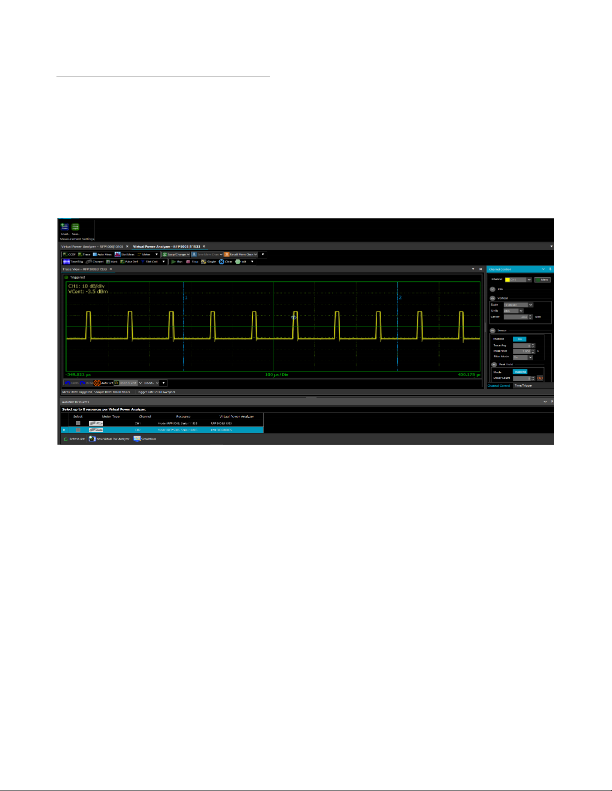
Operation 58
4.2.3 Multichannel Individual Sensor Tabs
Multiple sensors can also be employed individually. Starting with multiple sensors listed in the Available Resources window,
click on one sensor, then click the New Virtual Power Analyzer button. A Virtual Power Analyzer (VPA) tab will be
opened listing the model and serial number of the selected sensor.
Click on another sensor in the Available Resources window and then click on the New Virtual Power Analyzer button
again. A second VPA tab will be opened as shown in gure ??. This mode of multichannel operation treats each sensor
individually. Select a VPA tab and all the control windows apply only to the selected sensor. Each VPA Trace View will
show the selected sensor as Channel 1 (CH1). They are dierentiated by the model and serial number listed on the tab.
Likewise, all measurement windows will list measurements only for the selected sensor.
Figure 4.30 Mult-Cchannel Individual Sensor Tab
This creates two dierent instances of the Power Analyzer Software. To switch between them select the appropriate VPA
tab. There is no option to add a second sensor to an existing single-channel VPA. The only way to do that is to close
the VPA channel and restart as a multichannel VPA.
Page 59

Operation 59
4.3 Measurement Buer Mode(API remote programming only)
Measurement Buer Mode for the RFP Series Sensors works in conjunction with Real Time Power Processing™ to provide
all relevant burst information including timing, power and crest factor while eliminating the need to buer, download and
post-process large sample buers.
Measurement Buer Mode captures and analyzes the input signal during time intervals of interest and discards information
that occurs during non-relevant intervals. This mode of operation performs most analysis in real-time during capture.
The big advantage this measurement buer mode oers to the user is that it reduces the stream of sample data to a
single data record for each pulse, burst or event. Even for the fastest pulse rates, the data rate to the user is orders of
magnitude less than the sample data rate, so in most situations it becomes possible to store and transfer power analysis
results to the user in real time with no gaps in acquisition or analysis.
The Measurement Buer Mode circuitry can analyze and buer points at better than 2M buered points per second
(depending upon operating mode). The RFP Series Sensors internal measurement buer can capture, analyze and store
measurements for up to 2048 bursts at full rate. Additionally, a "circular" or FIFO capability allows continuous readout
of buered measurements by a host computer during capture and analysis. This real-time feature eectively removes
the 2048 point internal buer limitation, and permits capture and storage of test sequences of any size or duration to
an external host measurement buer. Continuous buered capture is possible at sustained rates of better than 100K
buered points per second to a host memory array or disk le.
4.3.1 Buer Overview
The RFP Series Sensors measurement buer consists of 2048 buer entries, each containing information about a unique
time interval.
Buer Entries. Each "Buer Entry" contains the following measurement values for that time interval:
Average interval power
Peak interval power
Minimum interval power
Interval start time (relative to start time of rst entry)
Interval duration (time from start to end of interval)
Entry count (buer reading number - increments each entry)
A 32-bit "Entry Count" counter (called “sequence number” in the IVI driver) keeps track of how many buer entries have
been processed and stored.
Page 60

Operation 60
Table 4.4 shows a sample measurement buer consisting of seven buer entries. In this example, the buer consists of
seven entries, each corresponding to a single burst.
Entry Count Interval Start Interval Duration Interval Average Interval Minimum Interval Peak
0 0.00 us 5.01 us -0.043 dBm -39.042 dBm 8.826 dBm
1 9.99 us 5.00 us -0.006 dBm -38.431 dBm 8.827 dBm
2 19.99 us 5.01 us 0.039 dBm -41.549 dBm 9.742 dBm
3 30.00 us 5.00 us 0.017 dBm -38.551 dBm 9.802 dBm
4 40.01 us 5.00 us 0.022 dBm -40.699 dBm 9.477 dBm
5 49.99 us 5.00 us -0.020 dBm -39.706 dBm 8.102 dBm
6 60.00 us 5.00 us 0.036 dBm -37.803 dBm 9.750 dBm
Table 4.4 Example of Measurements Stored in Buer
Figure 4.31 Sample Burst Signal
Buer Gates. The measurement interval for each Buer Entry is dened by a "gate" signal that controls the start and
end of data acquisition for that entry. At the start of each gate interval, a fresh acquisition interval is initiated, and at
the end of the gate, the acquisition interval is concluded and the result (the "buer entry"), as shown in Figure 4.25,
is written to memory. The gate signal may be internally or externally generated in several dierent ways - see "Gating
Modes" section below.
Buer Sessions. Each "Measurement Buer Session" consists of a series of acquired buer entries, stored in sequential
order to an onboard memory. The duration of a session may be monitored and controlled by user command, by an
external "run" signal, or limited to a preset number of entries or a preset time period. See "Session Arming" and "Session
AutoStop" sections below. In the example above, the session consists of seven buer entries, acquired over approximately
65 microseconds.
Page 61

Operation 61
4.3.2 Measurement Buer Mode Operation
Gating Modes. Each Buer Entry is controlled by a "buer gate" that denes the start and end of the entry time
interval. The gate signal may be internally or externally generated in several dierent ways.
Marker Gate: Each buer entry is "between markers" interval for one triggered sweep. This mode is used
with the power sensor operating in triggered pulse mode, and the sweep system and markers are used to dene
the start and end of each gate interval. The entire gate interval must fall within the limits of the visible trace,
so trigger and Time base settings must be appropriate for the signal.
Burst AutoGate: Each buer entry consists of a single pulse or burst. The start and end of the burst are
automatically identied by comparing the measured input signal to the trigger level threshold. Gate qualifying
and delay options are available to align the gate interval with the desired portion of a burst.
External Gate: Each buer entry consists of a single measurement interval gated by the logic state of the
Multi-I/O input. Qualifying and delay options are available to align the gate interval with the Multi-I/O input.
External Trigger Gate: Each buer entry is initiated by assertion of the Multi-I/O input and ends after a
user-dened duration. Qualifying and delay options are available to align the gate start with the Multi-I/O
input. If a qualied Multi-I/O assertion (rising edge) occurs prior to the programmed duration, the gate
interval in progress will end immediately and a new interval will begin with no gap between intervals.
Periodic Gate: Buer entries are self-timed intervals with user-dened period and duration. If period setting
is less than or equal to duration setting, the period setting will be used for both and there will be no gap
between successive intervals.
Acquisition of each entry begins upon assertion of the buer gate, and concludes upon de-assertion of the buer gate.
When the gate interval starts, a fresh accumulation of power samples begins. When the entry interval ends, the
accumulated power samples are processed to yield one set of avg/min/max and duration values for the entire interval,
and this result is stored to the next available buer location in memory.
Power samples are not accumulated when the gate is inactive. Buer entries (gates) may not overlap, however gap-less
buering (zero "gate inactive" time) is possible in certain modes. In this case, a new gate interval begins immediately
upon completion of the preceding gate interval.
Gate Qualify. If the Gate Mode is set for Burst AutoGate or External Gate/Trigger, additional criteria and time delays
may be imposed to aid in aligning the gated measurement on a desired signal interval. Start and End qualifying values
indicate the time that the controlling input (RF signal level or MIO external gate) must remain above or below the
qualifying threshold (trigger level for RF input, TTL levels for MIO) to be recognized.
The Start qualier can be used to reduce sensitivity to brief noise spikes while the burst is "o". Typically, the start
qualify time will be short - perhaps 10 to 50 ns.
The End qualier is commonly used to avoid premature burst end detection when burst modulation causes the RF
signal to briey fall below the qualifying threshold. For wideband modulation, this value must be longer than expected
modulation dips, but shorter than intra-burst gaps - typically 50 to 200 ns.
The internal gate signal is automatically adjusted to align with the beginning of recognized qualifying intervals - no user
adjustment is necessary. This means that the qualied gate which controls buering will correspond to the actual start
and end of the burst, and not be delayed by the qualifying times.
Gate Start/End Delay. If time adjustment of the qualied gate interval is needed to align the desired gate interval
with signal timing, the start and end times may be delayed by a user-controlled value. Gate delays may be positive or
negative to permit moving the gate interval ahead or back in time, respectively.
Page 62

Operation 62
A positive start delay can be used to exclude the rising edge of a burst, or to exclude a training sequence of known
duration. Similarly, a negative end delay will cause the qualied gate to end early, so can be used to exclude the falling
edge of a burst.
Since all processing is done in real-time, a built-in signal FIFO is used to permit the "look-back" action necessary to start
or end a gate interval prior to the qualifying event. Therefore, the dierence of the qualifying time and gate delay for
both the start and end gates cannot exceed the FIFO depth of 20 microseconds (implementation specic). This means
that if the end qualify time is 2 us, the end delay may be no more negative than -18 us. To simplify settings control, the
available time is split in half between the gate qualify and negative delay limits.
Figure 4.32 Gate Qualify and Delay
Figure 4.26 illustrates how gate qualify and delay options may be combined to align the desired buer gate with a signal
burst.
• The StartQualify time is set to 0.2 us so the start of the burst will only be recognized when the signal remains above
the gate threshold for 0.2 us or longer. This ensures that brief noise spikes while the burst is o are not recognized
as a valid burst.
• The EndQualify time is set to 1.0 us so the end of the burst will only be recognized when the signal remains below
the gate threshold for 1.0 us or longer. This ensures that brief modulation dips during the burst do not prematurely
end the gate interval.
• The StartDelay time is set to 0.5 us. This begins the gate interval 0.5 us after the beginning of the StartQualify
interval and is used to exclude rising edge eects such as transition time or overshoot from the gate measurement.
• The EndDelay time is set to -0.5 us. This ends the gate interval 0.5 us before the beginning of the EndQualify
interval and is used to exclude falling edge eects such as transition time from the gate measurement.
The entire qualied "burst interval" is 5 us long - starting and ending at the beginning of the StartQualify and EndQualify
times. The nal "gate interval" is oset at the start and end of the burst to exclude rising and falling edge eects.
Therefore, the measured "duration" stored in the buer for the 5 us burst shown will be about 4 us.
Page 63

Operation 63
Session Arming (Start) control. Although buered acquisition may be enabled ("running"), no data is collected unless
the session is "armed" to accept gate signals (see "Gating Modes"). Recognition of the selected gate signal is controlled
by arming or disarming the session.
When a session is armed, one buer entry will be written to the buer memory at the conclusion of each gate interval.
When the session is not armed, gate signals are ignored, and no entries are saved. This permits a session to be launched
or controlled via user software or an external signal.
The following settings are available to arm or control Measurement Buer sessions.
Immediate:
The session is armed immediately - each valid gate signal will generate a buer entry. The
session remains armed until disarmed by other means (see "Session Stop" below).
ExtStart:
The session is armed upon assertion of an external start (arming) pulse on the Multi-I/O.
Following arming, the buer system will remain armed, and each valid gate signal will generate
a buer entry. The session remains armed until disarmed by other means (see "Session Stop"
below).
ExtEnable:
The session is armed when the external enable signal to the Multi-I/O is asserted, and will
remain armed as long as the Multi-I/O is asserted. If the Multi-I/O is de-asserted, the system
disarms and sample acquisition halts. Asserting the Multi-I/O signal again re-arms and
continues collecting buer entries from the previous location - it does not reset the buer.
At the start of any Measurement Buer session, the buer status is reset. This clears the entry count and discards any
unread entries.
Session Auto-Stop conditions. Each Buer Session may be automatically terminated - this disarms the session so no
further entries are stored. Entries which have already been started are aborted without being written.
Automatic stop can occur in several ways:
Counted:
The current Measurement Buer session is terminated when "N" buer entries have been
acquired during that session.
Timed: The current Measurement Buer session is terminated "T" seconds after the start of the session.
ExtEnable:
The current Measurement Buer session is terminated upon de-assertion of an external buer
enable signal on the Multi-I/O.
Overow:
The current Measurement Buer session is terminated if the number of unread entries reaches
the capacity of the buer.
Note:
Auto-stop criteria are all examined. The session will terminate for whichever event occurs rst. The auto-stop criteria
can be disabled.
Page 64

Operation 64
Mbuf Enable Modes. Overall control of the Measurement Buer system is handled in much the same way as other
measurements - user controls for "Run", "Stop" and "Reset" are available.
MbufEnable=ON:
Reset the Measurement Buer system and enable a new Measurement Buer
session. Acquisition will begin with the rst buer entry once the system is
armed (see "Session Arming (Start) control") and a valid gate signal is received
(see "Gating Modes").
MbufEnable=OFF:
Halts any Measurement Buer session in progress. If the gate is currently active,
its acquisition data will be lost. This functions as a "stop" command and all
acquired buer data will still be available to read. Note that sessions may already
be stopped due to "auto-stop" conditions being met.
MbufReset
Halts and clears the Measurement Buersystem. This will force MbufEnable to
OFF. The read count and write index are returned to zero and no buer data will
be available to read.
Buer Read. Users may read the entire buer contents once the session is complete, or may read any newly acquired
entries while the buer session is in progress. User settings control the maximum number of entries to be returned for
each I/O read, up to the full capacity of the buer. However, the number of returned entries will be limited to the
number of "new" (acquired, unread) buer entries.
Each time the user reads entries from the buer, a read pointer is incremented by the number of entries returned, and
subsequent user reads will return new buer elements beginning with the rst unread entry.
Circular/Continuous Buer Acquisition. If the number of entries in a buer session reaches the end of the measurement
buer without stopping, buered acquisition will continue in circular fashion - that is entries will "wrap" and begin relling
the buer from the start.
Ordinarily, this would overwrite the buer contents, resulting in loss of acquired measurements. However, since users can
read buer sessions during acquisition, it is possible to periodically empty the buer so overwrite of old data does not
occur.
From a user perspective, the buer appears as a 2048 element FIFO. Provided the user avoids FIFO overow by reading
the buer periodically, the buer entries may be stored externally by the user to create buers of any size desired.
If the user is not able to read the buer before overow occurs, two options are available to control behavior:
Overow
Protection
ON:
Overow Protection ON: Enables auto-stop for pending buer overow. Buer entries continue
to be acquired in circular fashion provided the user periodically reads the buer. But if the buer
lls to capacity (2048 unread entries) without being emptied, the session is terminated and no
further entries are stored. This mode gives priority to the earliest acquired entries and ignores
events after the session terminates. DEFAULT MODE.
Overow
Protection
OFF:
Disables auto-stop for buer overow. Buer entries continue to be acquired in circular fashion without regard to read status by the user. If the buer lls to capacity (2048 unread entries)
without being emptied, new entries will continue to be stored, and will overwrite the oldest entries. This mode gives priority to the latest acquired entries, and discards older events whether or
not they have been read by the user.
Page 65

Operation 65
4.3.3 Measurement Buer Mode User Settings
The following settings, queries and controls are available with the applicable modes and argument options or numeric
ranges shown. Note that this is the SENSOR command interface, and may not align exactly with the API interface.
Please consult API documentation for available settings and queries.
Gate Settings
MbufGateMode
MbufGateStartQual
MbufGateStartDelay
MbufGateEndQual
MbufGateEndDelay
MbufGatePeriod
MbufGateDuration
Session Control Settings
MbufStartMode
MbufStopCount
MbufStopTime
MbufProtection
MbufEnable
MbufReset
[ MarkerGate BurstAutoGate ExtGate ExtTrigGate PeriodicGate ]
0.0 to 10 us
-10 us to 100 ms
0.0 to 10 us
10 us to 100 ms
100 ns to 10 s
100 ns to 100 ms
[ Immediate ExtStart ExtEnable ]
1 to 1M rdgs
1 ms to 1000 s
[on |o]
[on |o]
—
(BurstAutoGate, ExtGate and ExtTrigGate)
(BurstAutoGate, ExtGate and ExtTrigGate)
(BurstAutoGate and ExtGate)
(BurstAutoGate and ExtGate)
(PeriodicGate)
(ExtTrigGate and PeriodicGate)
(<=0 disables counted auto-stop)
(<=0 disables timed auto-stop)
Enables auto-stop for buer overwrite
"run/stop" control
Stops and resets the measurement buer session
Measbuf Readback Settings
MbufFetchCount
MbufAvailCount?
MbufFetchNext?
MbufFetchIndex[?]
Multi-I/O Priority: The RFP Series Sensors Multi-I/O connector may be used as input or output in several dierent
ways. When conicts occur, priority must be determined or undened behavior will result.
Multi-Channel Operation: When synchronized buering between multiple channels is required, the concept of "master"
and "slave" will again be needed to ensure gate intervals align between sensors. The "Trigger Source" logic can be used
here.
1 to 2048 Sets
Sets # of entries to be returned to user
Returns # of unread entries in MBUF
Returns next "MbufFetchCount " entries, incr ptr
Sets or returns current read pointer index
Page 66

Operation 66
In all congurations requiring a separate master and slave, the supplied "TriggerSync" cable must be used to interconnect
the Multi-I/O connectors of the master and all slaves. Where more than one slave is present, additional cables and a "T"
adapter will be needed for the parallel connection.
The Multi-I/O connector is not required by the Measurement Buer system in many Single-channel congurations
Mode Master Slave Required Connections
Marker
Gate
Burst
AutoGate
External
Gate
External
TrigGate
Pulse mode trigger out/arm status in signal to/from the MultiI/O connector. Mbuf gate signal
is internally generated by sweep
system in each sensor.
RF Burst is qualied/delayed by
master to create the Mbuf gate.
Master Multi-I/O outputs the
Mbuf gate to all slaves.
Pulse mode trigger in/arm status
out signal to/from Multi-I/O.
Mbuf gate signal internally generated by sweep system using
same marker settings as master,
so will be synchronized.
Multi-I/O receives qualied/delayed burst-detect signal from
master. Each slave operates in
"Ext Gate" Mbuf mode, so will
follow master.
There is no "master" or "slave" for this mode. All Multi-I/O inputs receive the ExtGate signal from a user source to gate each
Mbuf entry. Mbuf entries for all connected sensors start and end in
sync upon assertion and de-assertion of user ExtGate signal.
There is no "master" or "slave for this mode. All Multi-I/O inputs
receive the ExtTrigGate signal from a user source to initiate each
Mbuf entry. Mbuf entries for all connected sensors start in sync
upon assertion of user ExtTrigGate signal and end after user congured time duration.
Interconnect Multi-I/O inputs of
master and all slaves.
Interconnect Multi-I/O inputs of
master and all slaves.
Drive Multi-I/O inputs of all sensors from user-supplied External
Gate logic signal.
Drive Multi-I/O inputs of all sensors from user-supplied External
Gate logic signal.
Periodic
Gate
Master uses internal period and
duration timers to control start
and end of each Mbuf entry.
Multi-I/O of master outputs 100
ns "start pulse" at the start of
each Mbuf period.
Slaves operate in External Trigger Mbuf mode. All slave MultiI/O inputs receive the start pulse
from master to initiate each
Mbuf entry. Each slave times
the duration to end each entry.
Interconnect Multi-I/O inputs of
master and all slaves.
Table 4.5 Measurement Buer Functions and I/O Connections
Driver for RTP Sensors Functionality: The API for RTP Sensors exposes all of the measurement buer controls and
functions described in this section. However, for most use cases, the API oers a simplied set of methods and properties
to allow the user to specify an arbitrary number of measurements to capture. This allows the programmer to specify the
pertinent modes and gate qualications, acquire a user-specied number of measurements, and then retrieve the buered
measurement arrays.
For further information see the RTP Series Power Sensor Programming Reference.
Page 67

Remote Programming
The RFP Series Sensors can be remote controlled using an Application Programming Interface (API). The API for
RTP Sensors can be used by many programming environments and languages including C/C++, Python, Visual Basic,
Visual C#, LabVIEW, MATLAB, and others. This API permits user applications to access power sensor control and
measurement functions via a Dynamic Link Library (DLL). For more information, please see the RFP Series Power Sensor
Programming Reference.
5.1 Communication Overview
User software interfaces with the sensor via an Application Programming Interface (API). Settings and measurements can
be set and queried using functions and properties dened in the programming manual. The API communicates with the
sensor using low level calls to Microsoft’s Windows USB driver (WinUSB). WinUSB then sends and receives proprietary
binary commands and responses from the sensor. Figure 5.1 shows a graphical representation of the data ow between
a user application and an RFP Sensor.
Figure 5.1 Communication Data Flow
Page 68

Denitions & Measurements
This section provides denitions for key terms used in this manual and on the GUI displays as well as methodologies used
to calculate automated pulse, marker and statistical measurements.
6.1 Pulse Measurements
6.1.1 Pulse Denitions
IEEE Std 181™-2011 IEEE Standard for Transitions, Pulses, and Related Waveforms, provides fundamental
denitions for general use in time domain pulse technology. Several key terms dened in the standard are reproduced in
this subsection, which also denes the terms appearing in the RTP Series Real-Time Power Sensors text mode display of
automatic measurement results.
6.1.2 Standard IEEE Pulse
The key terms dened by the IEEE standard are abstracted and summarized below. These terms are referenced to the
standard pulse illustrated in gure 6.1.
Figure 6.1 IEEE Standard Pulse
Page 69

Denitions & Measurements 69
Note:
IEEE Std 194™-1977 IEEE Standard for Pulse Terms and Denitions has been superseded by IEEE Std
181™-2003 and -2011. Many of the terms used below have been deprecated by the IEEE. However, these terms are
widely used in the industry and familiar to users of power meters. For this reason, they are retained.
TERM DEFINITION
Base Line
Top Line The portion of a pulse waveform which represents the second nominal state of a pulse.
The two portions of a pulse waveform which represent the rst nominal state from which a
pulse departs and to which it ultimately returns.
First Transition
Last Transition
Proximal Line
Distal Line
Mesial Line
The major transition of a pulse waveform between the base line and the top line
(commonly called the rising edge).
The major transition of a pulse waveform between the top of the pulse and the base line.
(Commonly called the falling edge.)
A magnitude reference line located near the base of a pulse at a specied percentage
(normally 10%) of pulse magnitude.
A magnitude reference line located near the top of a pulse at a specied percentage
(normally 90%) of pulse magnitude.
A magnitude reference line located in the middle of a pulse at a specied percentage
(normally 50%) of pulse magnitude.
Table 6.1 Pulse Measurement Amplitude Threshold Terms
Page 70

Denitions & Measurements 70
6.1.3 Automatic Pulse Measurements
The RFP Series Sensors and the Power Analyzer Software or API automatically analyzes the waveform data in the buers
and calculates key waveform parameters. The calculated values are displayed in Auto Meas window.
Table 6.2 summarizes the automatic eld parameters available. Note that the Pulse Measurements can be edited and
customized. Amplitude related parameters will be displayed in the same units as selected in the Channel Control Window.
Field Label Parameter Denition
Width Pulse Width The interval between the rst and second signal crossings of the mesial line.
Rise Risetime
Fall Falltime
Period Pulse Period
PRF
Duty Duty Cycle The ratio of the pulse on-time to o-time.
Otime O-time
WavAv
PulsAv
PulsPk Pulse Peak Power
Droop Pulse Droop
Top
Bot
EdgDly Edge Delay
Skew
Pulse Repetition
Frequency
Waveform
Average Power
Pulse Average
On Power
IEEE Pulse
Top Amplitude
IEEE Pulse
Bottom Amplitude
Channel-to
Channel Skew
The rising edge time interval from the rst crossing of the proximal line to
the rst crossing of the distal line.
The falling edge time interval from the last crossing of the distal line to the
last crossing of the proximal line.
The time interval between two successive rising edges or two successive
falling edges. (Reciprocal of the Pulse Repetition Frequency)
The number of cycles of a repetitive signal that take place in one second.
The time a repetitive pulse is o. (Equal to the pulse period minus the pulse
width).
Waveform Average Power
The average “on” power level across the pulse width, dened by the intersection of the pulse rising and falling edges with the mesial line, and oset by
the StartGate and EndGate settings.
The maximum power level of the captured waveform OvrSht Overshoot
Leading edge overshoot (The dierence between the maximum amplitude
of the overshoot and the top line).
Rise or Droop in amplitude between the start and end of the pulse, as dened by the StartGate and EndGate settings.
The amplitude of the top line. (See IEEE denitions)
The amplitude of the base line. (See IEEE denitions)
The delay time relative to the trigger of the rst onscreen mesial level transition of either polarity. The Edge Delay value will be negative if the mesial
transition occurs before the trigger event, and positive if it occurs after the
trigger event.
The time between the mesial level of a pulse on Channel 1 and a pulse on
Channel 2. The pulse can be the power or trigger signal.
Table 6.2 Automatic Measurement Parameters
Page 71

Denitions & Measurements 71
6.1.4 Automatic Pulse Measurement Criteria
Automatic measurements are made on repetitive signals that meet the following conditions:
Amplitude: The dierence between the top and bottom signal amplitudes must exceed 6 dB to calculate
waveform timing parameters (pulse width, period, duty cycle). The top-to-bottom amplitude dierence must
exceed 13 dB to measure rise and falltime.
Timing: In order to measure pulse repetition frequency and duty cycle, there must be at least three signal
transitions. The interval between the rst and third transition must be at least 1/5 of a division (1/50 of the
screen width). For best accuracy on rise and falltime measurements, the timebase should be set so the transition interval is at least one- half division on the display.
6.1.5 Automatic Pulse Measurement Sequence
The automatic measurement process analyzes the captured signal data in the following sequence:
1. Approximately 500 samples of the waveform (equivalent to one screen width) are scanned to determine the maximum
and minimum sample amplitudes.
2. The dierence between the maximum and minimum sample values is calculated and stored as the Signal Amplitude.
3. The Transition Threshold is computed as one-half the sum of the maximum and minimum sample amplitudes.
Figure 6.2 Step Waveforms
4. The processor locates each crossing of the Transition Threshold.
5. Starting at the left edge of the screen, the processor classies each Transition threshold crossing according to whether
it is positive-going (– +) or negative-going (+ –). Because the signal is repetitive, only three transitions are needed
to classify the waveform, as shown in table 6.3.
Type Edge Sequence Description
0 none No crossings detected
1 Not used
2 + – One falling edge
3 – + One rising edge
4 + – + One falling, followed by one rising edge
5 – + – One rising, followed by one falling edge
6 + – + – Two falling edges
7 – + – + Two rising edges
Table 6.3 Waveform Classication Types
Page 72

Denitions & Measurements 72
6. If the signal is Type 0, (No crossings detected) no measurements can be performed and the routine is terminated,
pending the next reload of the measurement buers.
7. The process locates the bottom amplitude (baseline) using the IEEE histogram method. A histogram is generated
for all samples in the lowest 12.8 dB range of sample values. The range is subdivided into 64 power levels of 0.2
dB each. The histogram is scanned to locate the power level with the maximum number of crossings. This level is
designated the baseline amplitude. If two or more power histograms contain equal counts, the lower is selected.
8. The process follows a similar procedure to locate the top amplitude (top line). The power range for the top histogram
is 5 dB and the resolution is 0.02 dB, resulting in 250 levels. The level-crossing histogram is computed for a single
pulse, using the samples which exceed the transition threshold. If only one transition exists in the buer (Types 2
and 3), the process uses the samples that lie between the edge of the screen and the transition threshold as shown in
gure 6.2.
9. The process establishes the proximal, mesial, and distal levels as a percentage of the dierence between top amplitude
and bottom amplitude power. The percentage can be calculated on a power or voltage basis. The proximal, mesial,
and distal threshold values are user settable from 1% to 99%, with the restriction that the proximal < mesial < distal.
Normally, these values will be set to 10%, 50% and 90%, respectively.
10. The process determines horizontal position, in pixels, at which the signal crosses the mesial value. This is done to
a resolution of 0.1 pixel, or 1/5000 of the screen width. Ordinarily, the sample values do not fall precisely on the
mesial line, and it is necessary to interpolate between the two nearest samples to determine where the mesial crossing
occurred. This process is illustrated in the example shown in gure 6.3.
Figure 6.3 Time Interpolation Example
Item dBm mW
Mesial value 10.0 10.0
Sample n 8.0 6.3
Sample n + 1 11.0 12.6
Table 6.4 Time Interpolation Example
Page 73

Denitions & Measurements 73
The interpolated crossing time, tx, is calculated as follows:
𝑡𝑥 = 𝑡𝑛 +
where P is in watts and n is the number of the sampling interval, referenced to the trigger event.
For this example:
𝑡𝑥 = 𝑡𝑛 +
11. The processor computes the rise and/or falltimes of waveforms that meet the following conditions:
– The waveform must have at least one usable edge (Types 2 through 7, as shown in table 6.4)
– The signal peak must be at least 13 dB greater than the minimum sample value.
The risetime is dened as the time between the proximal and distal crossings (– +).
The falltime is dened as the time between the distal and proximal crossings (+ –).
If no samples lie between the proximal and distal values for either edge (rise or fall), the risetime for that edge is set
to 0 seconds.
12. The processor calculates the output values if applicable according to the following denitions:
– Pulse Width Interval between rising and falling edge mesial points
– Risetime See Step 11
– Falltime See Step 11
𝑃𝑚𝑒𝑠 − 𝑃𝑛
𝑃𝑛 + 1 − 𝑃𝑛
10.0 − 6.3
12.6 − 6.3
= 𝑡𝑛 + 0.6
– Period Cycle time between successive mesial points of the same polarity
– Pulse Repetition Frequency Reciprocal of Period
– Duty Cycle Pulse Width/Period
– O-time (Period) - (Pulse Width)
– Peak Power Maximum sample value between StartGate time and EndGate time (See Step 1)
– Pulse Power Average power between StartGate time and EndGate time
– Overshoot (Peak Power) - (Top Amplitude)
– Average Power See Step 13
– Top Amplitude See Step 8
– Bottom Amplitude See Step 7
– Droop between StartGate time and EndGate time
– Skew See Step 14
Page 74

Denitions & Measurements 74
6.2 Marker Measurements
Table 6.5 summarizes the Marker Measurements available. Note that the Marker Measurements can be edited and
customized. Amplitude related measurements will be displayed in the same units as selected in the Channel Control
window.
Field Label Parameter Denition
MkAvg Marker Average Average power over marker interval
MkMin Marker Minimum Minimum instantaneous power over marker interval
MkMax Marker Maximum Maximum instantaneous power over marker interval
MkMaxF Marker Maximum Filtered Maximum average (ltered) power over marker interval
MkMinF Marker Minimum Filtered Minimum average (ltered) power over marker interval
MkPk2A Marker Peak to Average Peak-to-Average power ratio over marker interval
Mk1Lvl Marker 1 Level Average power at marker 1
Mk2Lvl Marker 2 Level Average power at marker 2
MkMaxAv Marker Max Interval Average Highest value of average-between-markers
MkMinAv Marker Min Interval Average Lowest value of average-between-markers
Mk1Min Marker 1 Minimum Minimum power or voltage at the Marker 1
Mk1Max Marker 1 Maximum Maximum power or voltage at the Marker 1
Mk2Min Marker 2 Minimum Minimum power or voltage at the Marker 2
Mk2Max Marker 2 Maximum Maximum power or voltage at the Marker 2
MkRatio Marker Ratio Ratio of Marker 1 to Marker 2
MkDelta Marker Amplitude Dierence Amplitude dierence between Marker 1 and Marker 2
MkRDelta Marker Reverse Dierence Amplitude dierence between Marker 2 and Marker 1
MkRRatio Marker Reverse Ratio Ratio of Marker 2 to Marker 1
Mk1Time Marker 1 Time Time at Marker 1
Mk2Time Marker 2 Time Time at Marker 2
MkTimeDelt Marker Time Dierence Time Dierence between Marker 1 and Marker 2
Table 6.5 Marker Measurements
Page 75

Denitions & Measurements 75
6.2.1 Average Power Over a Time Interval
13. The average power of the signal over a time interval is computed by:
– Summing the power values at each point within the interval
– Dividing the sum by the number of points
This process is used to calculate Pulse Power, Average Power and the average power between markers.
Since each point represents the power over a nite time interval, the endpoints are handled separately to avoid
spreading the interval by one-half pixel at each end of the interval (See gure 6.4 ). For the interval in gure 6.4,
the average power is given by:
𝑛−1
1
∑
𝑛=1
𝑎𝑣𝑒
1
=
(𝑃0 + 𝑃𝑛) +
2
(𝑛 − 1)
𝑃
Figure 6.4 Sampling Intervals
14. To compute channel-to-channel Skew, the processor calculates the delay between the two measurement channels. The
time reference for each channel is established by the rst signal crossing (starting from the left edge of the screen)
which passes through the mesial level (or 50% point in trigger view). The signal excursion must be at least 6 dB.
Page 76

Denitions & Measurements 76
6.3 Automatic Statistical Measurements
Statistical Measurements based on the CCDF Graph are summarized in table 6.6
Field Label Parameter Denition
10% Power at 10% probability Peak to average power corresponding to 10% probability
1% Power at 1% probability Peak to average power corresponding to 1% probability
0.1% Power at 0.1% probability Peak to average power corresponding to 0.1% probability
0.01% Power at 0.01% probability Peak to average power corresponding to 0.01% probability
0.001% Power at 0.001% probability Peak to average power corresponding to 0.001% probability
0.0001% Power at 0.0001% probability Peak to average power corresponding to 0.0001% probability
Pct at 0 dB Probability (percent) at 0 dB Probability corresponding to 0 dB on the CCDF Graph
Cursor Pct Cursor Probability (percent) Probability at the Cursor Position on the CCDF Graph
Cursor Pwr Cursor Power
Average Average
Max Maximum
Min Minimum
Peak/Avg Peak/Average
Dynamic Range Dynamic Range The ratio (in dB) of the Peak Power to the Minimum Power
Peak to average power at the Cursor position on the CCDF
Graph
The unweighted average of all power samples occurring since
acquisition started
The highest power sample occurring since acquisition was
started
The lowest power sample occurring since acquisition was
started
Ratio The ratio (in dB) of the Peak Power to the Average
Power
Table 6.6 Automatic Statistical Measurements
Page 77

Maintenance
This section presents procedures for maintaining the RTP Series Real-Time Power Sensors.
7.1 Safety Recommendation
The RFP Series Sensors have been designed in accordance with international safety standards. General safety precautions
must be observed during all phases of operation and maintenance. Failure to comply with the precautions listed in the
Safety Summary located in the front of this manual could result in serious injury or performance issues. Service and
adjustments should be performed only by qualied service personnel.
Below are the safety recommendations for the RFP Series Sensors:
– Only rotate the connector nut, DO NOT use the sensor body or device to tighten the connector.
– Do not overtighten the RF connector.
– Do not use a connector with deformed threads, or a bent or broken conductor.
– Do not touch mating-plane surfaces with oily, or wax-like non-conductive substances.
– Do not apply a lateral force to the center conductor.
7.2 Cleaning
Painted surfaces and the RF connector can be cleaned very carefully with a mild cleaning solution (a solution of pure
isopropyl or ethyl alcohol). Keep in mind its ammable nature. Clean water dampened in cloth can be used to clean the
body of the RFP Series Sensors.
Note:
When cleaning the power sensor, do not allow any liquid to enter into the device.
Avoid using chemical cleaning agents which can damage painted or plastic surfaces.
7.3 Inspection and Performance Verication
If an RFP Series Sensor malfunctions, perform a visual inspection of the instrument. Inspect for signs of damage caused by
excessive shock, vibration or overheating. Inspect for broken or damaged connection port at sensor head, or accumulations
of dust or other foreign matter. Correct any problems you discover and verify basic functionality with the Power Analyzer
Software.
If desired, conduct a performance verication according to the procedure in the RFP Series Sensors Calibration and
Verication Guide to verify that the instrument is properly recognized by the Windows OS and operational. If the
malfunction persists or the sensor device fails the performance verication, contact BK Precision for service.
7.4 Connector Care
The most common cause of power sensor problems is excess input power. Applying power exceeding the labeled damage
levels will damage the sensing elements such that its voltage versus power relationships are changed, resulting in erroneous
Page 78

Maintenance 78
power readings.
The other most common cause of power sensor problems is damaged connectors. Connections should be tightened with
the proper torque wrench applied to the coupling nut only. Any attempt to torque or un-torque a connection using the
body of the power sensor may result in either connector damage, or in the connector becoming unthreaded from the
body.
The following handling precautions must be observed to prevent connector damage when using the RFP Series Real
Sensors.
– Keep connectors clean and protect using the plastic end caps provided with each sensor.
– Inspect connectors regularly and look for metal debris, scratches or dents.
– Clean contact surface and threads with clean, dry compressed air.
– Align connectors rst and only rotate the connector nut.
– A precision type “N” connector is recommended for the RF line signal source connection.
– After proper alignment, rotate the connector nut by hand to connect or disconnect the connector of the sensor from
a signal source as shown in gure 7.1.
Figure 7.1 Connecting Type-N(f) to Type-N(male)
– If the connector nut is not equipped with a hex, it should be hand tightened only.
– Do not over-tighten the connector by using the sensor body for additional leverage.
– Avoid mechanical shock.
– Avoid applying excessive power.
– Observe proper ESD (electrostatic discharges) precautions
Page 79
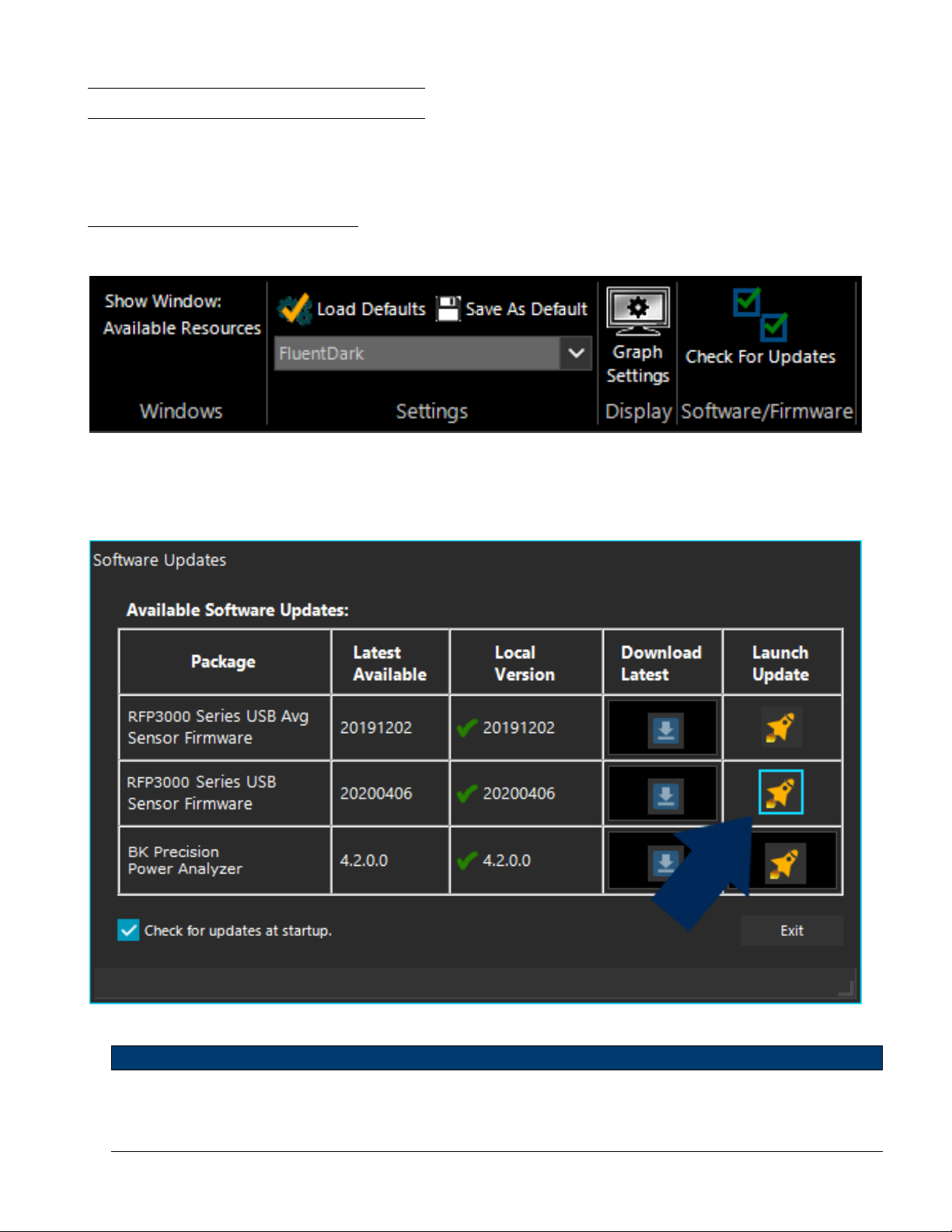
Maintenance 79
7.5 Software and Firmware Updates
The Power Analyzer Software includes the ability to check online for updates to both itself and the rmware in
connected RFP Series Sensors.
7.5.1 Firmware Update Procedure
1. On the main menu bar select the View tab then click the Check For Updates button.
Figure 7.2 Check for Updates
2. The Software Updates pop-up will appear. In the row labeled RFP Series … Firmware, click the Launch button.
Figure 7.3 Software Updates pop-up
Note:
Firmware current with the release of the Power Analyzer Software is embedded in the program and does not have to
be downloaded.
Page 80

Maintenance 80
3. If multiple RFP Series Sensor are connected the Select Sensor pop-up will appear. Select the desired sensor from
the drop-down menu and click OK.
Figure 7.4 Select Sensor
4. The Firmware Update pop-up will appear. If only one sensor is connected upon clicking the Launch button the
Firmware Update pop-up will appear without having to select a sensor.
Figure 7.5 Firmware Update Progress Bar
Page 81

Maintenance 81
5. Following successful rmware update, a status dialog will be displayed.
Figure 7.6 Firmware Update Succeeded
If the rmware is up to date the Up to Date pop-up will appear.
Figure 7.7 Up to Date
Page 82

Maintenance 82
7.5.2 Power Analyzer Software Update Procedure
1. On the main menu bar select the View tab then click the Check for Updates button.
pop-up
Figure 7.8 Check for Updates
2. The Available Software Updates pop-up will appear. In order to upgrade the software, download the update. In
the row labeled BK Precision Power Analyzer, click the Download button.
Figure 7.9 Download the Power Analyzer Software
Page 83

Maintenance 83
3. A save le dialog box will appear. Choose the location you wish to save the software update.
Figure 7.10 Saving the Software Update
4. The following message will appear when the download completes.
Figure 7.11 Save Complete
Page 84

Maintenance 84
5. Click the Launch button to begin the upgrade.
Figure 7.12 Launch the Power Analyzer Software Update
A progress bar will appear in the Launch column. Before the upgrade begins, the update package must be unzipped.
This process will take several minutes.
The installer will begin. Follow the prompts to complete the installation.
7.5.3 Checking for New Firmwarr After the Initial Installation
When new features are added to the Power Analyzer Software, a sensor rmware update is sometimes required to
fully support the new capabilities. After the update of the Power Analyzer Software, it is recommended that users
check for new rmware using the following procedure.
1. On the main menu bar select the View tab then click the Check for Updates button.
Figure 7.13 Check for Updates
Page 85

Maintenance 85
2. If a new version of rmware is available, there will be a yellow triangle with an exclamation point next to the version
under Local Version.
3. To begin downloading the newest rmware images, click the download button.
Figure 7.14 Check for Updates
A progress bar will appear in the “Download” column. This process may take several minutes.
4. Once the download is complete, a green check mark will appear next to the rmware version number.
Page 86

Maintenance 86
Figure 7.15 Firmware is Up to Date
Page 87

Specications
Page 88

Specications 88
Page 89

Service Information
Warranty Service: Please go to the support and service section on our website at bkprecision.com to obtain an RMA
#. Return the product in the original packaging with proof of purchase to the address below. Clearly state on the RMA
the performance problem and return any leads, probes, connectors and accessories that you are using with the device.
Non-Warranty Service: Please go to the support and service section on our website at bkprecision.com to obtain an
RMA #. Return the product in the original packaging to the address below. Clearly state on the RMA the performance
problem and return any leads, probes, connectors and accessories that you are using with the device. Customers not on
an open account must include payment in the form of a money order or credit card. For the most current repair charges
please refer to the service and support section on our website.
Return all merchandise to B&K Precision Corp. with prepaid shipping. The at-rate repair charge for Non-Warranty
Service does not include return shipping. Return shipping to locations in North America is included for Warranty Service.
For overnight shipments and non-North American shipping fees please contact B&K Precision Corp.
Include with the returned instrument your complete return shipping address, contact name, phone number and description
of problem.
B&K Precision Corp.
22820 Savi Ranch Parkway
Yorba Linda, CA 92887
bkprecision.com
714-921-9095
Page 90

LIMITED THREE-YEAR WARRANTY
B&K Precision Corp. warrants to the original purchaser that its products and the component parts thereof, will be free
from defects in workmanship and materials for a period of three years from date of purchase.
B&K Precision Corp. will, without charge, repair or replace, at its option, defective product or component parts. Returned
product must be accompanied by proof of the purchase date in the form of a sales receipt.
To help us better serve you, please complete the warranty registration for your new instrument via our website www.bkprecision.com
Exclusions: This warranty does not apply in the event of misuse or abuse of the product or as a result of
unauthorized alterations or repairs. The warranty is void if the serial number is altered, defaced or removed.
B&K Precision Corp. shall not be liable for any consequential damages, including without limitation damages resulting
from loss of use. Some states do not allow limitations of incidental or consequential damages. So the above limitation
or exclusion may not apply to you.
This warranty gives you specic rights and you may have other rights, which vary from state-to-state.
B&K Precision Corp.
22820 Savi Ranch Parkway
Yorba Linda, CA 92887
www.bkprecision.com
714-921-9095
Version: July 8, 2021
 Loading...