

Page 1

Page 2

Safety Summary
The following safety precautions apply to both operating and maintenance personnel and must be followed during all
phases of operation, service, and repair of this instrument.
Before applying power to this instrument:
• Read and understand the safety and operational information in this manual.
• Apply all the listed safety precautions.
• Verify that the voltage selector at the line power cord input is set to the correct line voltage. Operating the instrument
at an incorrect line voltage will void the warranty.
• Make all connections to the instrument before applying power.
• Do not operate the instrument in ways not specied by this manual or by B&K Precision.
Failure to comply with these precautions or with warnings elsewhere in this manual violates the safety standards of design,
manufacture, and intended use of the instrument. B&K Precision assumes no liability for a customer’s failure to comply
with these requirements.
2
Category rating
The IEC 61010 standard denes safety category ratings that specify the amount of electrical energy available and the
voltage impulses that may occur on electrical conductors associated with these category ratings. The category rating is
a Roman numeral of I, II, III, or IV. This rating is also accompanied by a maximum voltage of the circuit to be tested,
which denes the voltage impulses expected and required insulation clearances. These categories are:
Category I (CAT I): Measurement instruments whose measurement inputs are not intended to be connected to the
mains supply. The voltages in the environment are typically derived from a limited-energy transformer or a battery.
Category II (CAT II): Measurement instruments whose measurement inputs are meant to be connected to the mains
supply at a standard wall outlet or similar sources. Example measurement environments are portable
tools and household appliances.
Category III (CAT III): Measurement instruments whose measurement inputs are meant to be connected to the mains
installation of a building. Examples are measurements inside a building’s circuit breaker panel
or the wiring of permanently-installed motors.
Category IV (CAT IV): Measurement instruments whose measurement inputs are meant to be connected to the primary
power entering a building or other outdoor wiring.
Do not use this instrument in an electrical environment with a higher category rating than what is specied in this manual
for this instrument.
You must ensure that each accessory you use with this instrument has a category rating equal to or higher than the
instrument’s category rating to maintain the instrument’s category rating. Failure to do so will lower the category rating
of the measuring system.
Page 3

Electrical Power
This instrument is intended to be powered from a CATEGORY II mains power environment. The mains power should be
115 V RMS or 230 V RMS. Use only the power cord supplied with the instrument and ensure it is appropriate for your
country of use.
Ground the Instrument
To minimize shock hazard, the instrument chassis and cabinet must be connected to an electrical safety ground. This
instrument is grounded through the ground conductor of the supplied, three-conductor AC line power cable. The power
cable must be plugged into an approved three-conductor electrical outlet. The power jack and mating plug of the power
cable meet IEC safety standards.
Do not alter or defeat the ground connection. Without the safety ground connection, all accessible conductive parts
(including control knobs) may provide an electric shock. Failure to use a properly-grounded approved outlet and the
recommended three-conductor AC line power cable may result in injury or death.
3
Unless otherwise stated, a ground connection on the instrument’s front or rear panel is for a reference of potential only
and is not to be used as a safety ground. Do not operate in an explosive or ammable atmosphere.
Do not operate the instrument in the presence of ammable gases or vapors, fumes, or nely-divided particulates.
The instrument is designed to be used in oce-type indoor environments. Do not operate the instrument
• In the presence of noxious, corrosive, or ammable fumes, gases, vapors, chemicals, or nely-divided particulates.
• In relative humidity conditions outside the instrument’s specications.
• In environments where there is a danger of any liquid being spilled on the instrument or where any liquid can condense
on the instrument.
• In air temperatures exceeding the specied operating temperatures.
• In atmospheric pressures outside the specied altitude limits or where the surrounding gas is not air.
• In environments with restricted cooling air ow, even if the air temperatures are within specications.
• In direct sunlight.
This instrument is intended to be used in an indoor pollution degree 2 environment. The operating temperature range is
0∘C to 40∘C and 20% to 80% relative humidity, with no condensation allowed. Measurements made by this instrument
may be outside specications if the instrument is used in non-oce-type environments. Such environments may include
rapid temperature or humidity changes, sunlight, vibration and/or mechanical shocks, acoustic noise, electrical noise,
strong electric elds, or strong magnetic elds.
Page 4

Do not operate instrument if damaged
If the instrument is damaged, appears to be damaged, or if any liquid, chemical, or other material gets on or inside the
instrument, remove the instrument’s power cord, remove the instrument from service, label it as not to be operated,
and return the instrument to B&K Precision for repair. Notify B&K Precision of the nature of any contamination of the
instrument.
Clean the instrument only as instructed
Do not clean the instrument, its switches, or its terminals with contact cleaners, abrasives, lubricants, solvents, acids/bases,
or other such chemicals. Clean the instrument only with a clean dry lint-free cloth or as instructed in this manual. Not
for critical applications
This instrument is not authorized for use in contact with the human body or for use as a component in a life-support
device or system.
4
Do not touch live circuits
Instrument covers must not be removed by operating personnel. Component replacement and internal adjustments must
be made by qualied service-trained maintenance personnel who are aware of the hazards involved when the instrument’s
covers and shields are removed. Under certain conditions, even with the power cord removed, dangerous voltages may
exist when the covers are removed. To avoid injuries, always disconnect the power cord from the instrument, disconnect
all other connections (for example, test leads, computer interface cables, etc.), discharge all circuits, and verify there
are no hazardous voltages present on any conductors by measurements with a properly-operating voltage-sensing device
before touching any internal parts. Verify the voltage-sensing device is working properly before and after making the
measurements by testing with known-operating voltage sources and test for both DC and AC voltages. Do not attempt
any service or adjustment unless another person capable of rendering rst aid and resuscitation is present.
Do not insert any object into an instrument’s ventilation openings or other openings.
Hazardous voltages may be present in unexpected locations in circuitry being tested when a fault condition in the circuit
exists.
Fuse replacement must be done by qualied service-trained maintenance personnel who are aware of the instrument’s fuse
requirements and safe replacement procedures. Disconnect the instrument from the power line before replacing fuses.
Replace fuses only with new fuses of the fuse types, voltage ratings, and current ratings specied in this manual or on
the back of the instrument. Failure to do so may damage the instrument, lead to a safety hazard, or cause a re. Failure
to use the specied fuses will void the warranty.
Servicing
Page 5

Do not substitute parts that are not approved by B&K Precision or modify this instrument. Return the instrument to
B&K Precision for service and repair to ensure that safety and performance features are maintained.
For continued safe use of the instrument
• Do not place heavy objects on the instrument.
• Do not obstruct cooling air ow to the instrument.
• Do not place a hot soldering iron on the instrument.
• Do not pull the instrument with the power cord, connected probe, or connected test lead.
• Do not move the instrument when a probe is connected to a circuit being tested.
Compliance Statements
Disposal of Old Electrical & Electronic Equipment (Applicable in the European Union and other European
countries with separate collection systems)
This product is subject to Directive 2002/96/EC of the European Parliament
and the Council of the European Union on waste electrical and electronic equipment
(WEEE), and in jurisdictions adopting that Directive, is marked as being put on the
market after August 13, 2005, and should not be disposed of as unsorted municipal
waste. Please utilize your local WEEE collection facilities in the disposition of this
product and otherwise observe all applicable requirements.
5
Page 6

Safety Symbols
Symbol Description
indicates a hazardous situation which, if not avoided, will result in death or serious injury.
indicates a hazardous situation which, if not avoided, could result in death or serious injury
indicates a hazardous situation which, if not avoided, will result in minor or moderate injury
Refer to the text near the symbol.
Electric Shock hazard
Alternating current (AC)
Chassis ground
Earth ground
This is the In position of the power switch when instrument is ON.
This is the Out position of the power switch when instrument is OFF.
is used to address practices not related to physical injury.
6
Page 7

Contents
1 General Information 9
1.1 Organization 9
1.2 Description 10
1.3 Features 10
1.4 Front Panel 11
1.5 Rear Panel 13
1.6 Touch Screen Display 14
2 Installation 17
2.1 Contents 17
2.2 Input Power & Fuse Requirements 17
2.3 Connections 18
2.4 Preliminary Check 18
3 Getting Started 20
3.1 Initialization 20
3.2 Taking Measurements 22
3.2.1 Continuous Mode 22
3.2.2 Pulse Mode 23
3.2.3 Statistical Mode 24
4 Operation 26
4.1 Control Menus 26
4.2 Parameter Date Entry and Selection 26
4.2.1 Numerical Data Entry & Drop Down Menus 26
4.3 Menu Reference 27
4.3.1 Main Menu 27
4.3.2 Measure > 28
4.3.3 Display > 29
4.3.4 Stat. Mode > 29
4.3.5 Channel > 30
4.3.6 Channel Settings 31
4.3.7 Time > 34
4.3.8 Trigger > 34
4.3.9 Pulse Def. > 36
4.3.10 CH# Pulse Def 36
4.3.11 Favorites > 38
4.3.12 System > 38
5 Application Notes 42
5.1 Introduction to Pulse Measurements 42
5.1.1 Measurement Fundamentals 42
5.1.2 Diode Detection 44
5.1.3 Pulse Denitions 46
5.1.4 Standard IEEE Pulse 46
5.1.5 Automatic Measurements 47
5.1.6 Automatic Measurement Criteria 47
5.1.7 Automatic Measurement Terms 48
5.1.8 Automatic Measurement Sequence 49
5.1.9 Average Power Over an Interval 52
5.1.10 Statistical Mode Automatic Measurements 53
5.2 Measurement Accuracy 54
Page 8

6 Maintenance 55
6.1 Safety 55
6.2 Cleaning 55
6.3 Inspection 55
6.4 Lithium Battery 56
6.5 Software Upgrade 56
7 Service Information 57
8 LIMITED THREE-YEAR WARRANTY 58
8
Page 9

General Information
This instruction manual provides you with the information you need to install, operate, and maintain the RFM3000 RF
Power Meter. Section 1 is an introduction to the manual and the instrument.
1.1 Organization
The manual is organized into ve sections and two Appendices, as follows:
Section 1
General Information presents summary descriptions of the instrument and its principal features, acces-
sories, and options.
Section 2
Section 3
Section 4
Section 5
Installation provides instructions for unpacking the instrument, setting it up for operation, connecting
power and signal cables, and initial power-up.
Getting Started describes the controls and indicators and the initialization of operating parameters.
Several practice exercises are provided to familiarize yourself with essential setup and control procedures.
Operation describes the display menus and procedures for operating the instrument locally from the
front panel.
Application Notes provides supplementary information about RFM3000 and sensor operation, advanced features, pulse measurement information, and measurement accuracy.
Page 10

General Information 10
1.2 Description
The RFM3000 provides design engineers and technicians the utility of traditional benchtop instruments, the exibility
and performance of modern USB RF power sensors, and the simplicity of a multi-touch display built with advanced
technology.
As a benchtop meter, the RFM3000 provides a standalone solution for capturing, displaying, and analyzing peak and
average RF power in both the time and statistical domains through an intuitive, touch screen display.
The RFM3000 RF Power Meter utilizes up to four RFP Series Sensors with industry-leading performance and capabilities
either independently or for synchronized multi-channel measurements of CW, modulated, and pulsed signals.
Providing the ultimate exibility, the RFM3000 sensors can be disconnected and independently used as standalone
instruments.
1.3 Features
• Compatible with B&K Precision’s RFP3000 Series USB RF Power Sensors
• Capture/display/analyze peak and average power
• Independent or synchronous multi-channel measurements (up to 4 channels)
• Trigger synchronization
• Supports SCPI-1999.0
• Sensor verication test source
• Display 16 common power measurements
• Ethernet:10/100/1000 BaseT; HiSLIP
• HDMI output for mirror display
• Sensors can be used as standalone instruments
Page 11

General Information 11
1.4 Front Panel
Refer to table 1.1 for a description of each of the illustrated items. The function and operation of all controls, indicators,
and connectors are the same on the standard and optional models.
Figure 1.1 Front Panel
Page 12

General Information 12
Item Description
Four sensor inputs are located on the front and rear panels of the instrument. These are stan-
1 USB Host
dard USB 2.0 Type A receptacles designed to accept only RFP3000 Series Sensors or standard
USB keyboards, mice, and ash drives.
Four sensor trigger inputs are located on the front and rear panels of the instrument. These
are standard SMB receptacles designed to accept only BK Precision power sensor trigger ca-
2 Sync Ports
bles.
Do not attempt to connect anything other than RFP3000
sensors and trigger cables!
The output of the built-in 50 MHz programmable test source is available from a Type-N
3 RF Output
connector located on the front, or optionally on the rear panel of the instrument. This test
source is used to verify basic performance of sensors used with the RFM3000.
4 Display Screen
5
6
7
8
Color touch screen display for the measurement and trigger channels, screen menus, status
messages, text reports, and help screens.
Favorites key. (This function is not fully implemented at this time). Enables the user to setup
a customized menu to allow grouping frequently used menu items into one convenient menu.
Store image key saves a screen image of the meter to local storage. The images can be
copied to an external USB storage device.
Used to assist navigating between items on the display and in the menus. Unless the user is
in digit editing numeric entry mode.
Used for incrementing or decrementing numeric parameters, or scrolling through multi-line or
multi-page displays.
Selects an on-screen item or menu and completes a numeric or picklist entry
Toggles the instrument between “on” (fully powered) and “standby” (o, except for certain
low-power internal circuits) modes. Entering standby mode will perform a save of the current
instrument state before shutdown. Pressing and holding the On/Standby key for several seconds will force standby mode if the instrument has become non-responsive. In this case, no
context save is performed
Table 1.1 Front Panel
Page 13

General Information 13
1.5 Rear Panel
Refer to table 1.2 for a description of each of the illustrated items. The function and operation of all controls, indicators,
and connectors are the same on the standard and optional models.
Figure 1.2 Rear Panel
Page 14
General Information 14
Item Description
Four sensor inputs are located on the front and rear panels of the instrument. These are stan-
1 USB Host
2 Sync Ports
3 RF Output
4 Trig In
dard USB 2.0 Type A receptacles designed to accept only RFP3000 Series Sensors or standard
USB keyboards, mice, and ash drives.
Four sensor trigger inputs are located on the front and rear panels of the instrument. These
are standard SMB receptacles designed to accept only BK Precision power sensor trigger cables.
Do not attempt to connect anything other than RFP3000
sensors and trigger cables!
The output of the built-in 50 MHz programmable test source is available from a Type-N
connector located on the front, or optionally on the rear panel of the instrument. This test
source is used to verify basic performance of sensors used with the RFM3000.
BNC input for connecting an external trigger signal to the power meter. Voltage range is±5
volts, but the input impedance is 1 Megohm to allow use of common 10x oscilloscope probe
for a±50 volt input range.
5 Multi-I/O
6 LAN Ethernet
7 HDMI
8 AC Line Input
9 HDMI Cooling air intake.
10 GPIB
BNC input/output for exible use. May serve as a status or alarm output, signal level monitor, or settable voltage source
LAN connector for remote control and rmware updates. Allows DHCP or xed (IP / Subnet) setting mode. LAN parameters can be congured through the menu.
HDMI receptacle for connecting an external monitor to mirror front panel display. The image
resolution will be 800 x 480 and will be stretched to t the external full display size.
A multi-function power input module is used to house the AC line input, main power switch,
and safety fuse. The module accepts a standard AC line cord, included with the power meter.
The power switch is used to shut o main instrument power. The safety fuse may also be accessed once the line cord is removed. The instrument’s power supply accepts 90 to 264 VAC,
so no line voltage selection switch is necessary.
24-pin GPIB (IEEE-488) connector for connecting the power meter to the remote control
General Purpose Instrument Bus. GPIB parameters can be congured through the menu.
Replace fuse only with specied type and rating:
1.0A-T (time delay type), 250 VAC.
Table 1.2 Rear Panel
1.6 Touch Screen Display
The RFM3000 can be controlled through the touch screen display and by use of the front panel buttons. Table 1.3
describes the dierent areas of the display layout of the RFM3000. Figure 1.3 shows the Graph Display mode of the
instrument using the Pulse Measure mode with a menu exposed. Figure 1.4 shows the same measure mode with the
Page 15

General Information 15
menus hidden. The Text Display mode of the instrument provides a table view of measured parameters. Parameters
depend on the Measure mode selected. See Section Menu Referencefor more information on the display format.
Figure 1.3 Display
Figure 1.4 Display Hidden Menu
Page 16

General Information 16
Item Description
Indicates the measurement acquisition status of the unit. In Pulse mode, the sample rate and
1 Status Bar
number of sweeps per second are also shown. In Statistical mode, it indicates the gating setting in use, run time, and number of points.
Displays a table of measurements for each channel that is enabled on the meter. In Pulse and
2 Parameters
Continuous mode, measurements indicated are for power levels at each marker and the average power between the markers. For Statistical mode, the measurements are Average power,
Maximum power, and Peak-to-Average Ratio or Crest Factor.
This area indicates which channels are ON and their individual scale and vertical center.
3 Channel Status
The base RFM3000 model only permits two sensors to be
active at any one time. With the RFM300-4CH
option, four sensors can be active at any one time.
4 Main Display
5 Menu Bar
This area will show a plot when in Graph Display mode or a table of parameters when in Text
Display mode for the measurement mode selected.
Select to show and to hide the on-screen menus.
6 Menu Parth Used to navigate the menu structure. Shows the menu that will be displayed when selected.
7
Current
Menu/Home
8 Horizontal Scale
9 Measure Mode
Displays the name of the current menu and provides a home shortcut to the top-level Main
menu. When in the Main or top level menu, this eld is not available.
For Pulse and Continuous mode, indicates the time per division for the waveform display. In
Statistical mode, the horizontal scale for the CCDF graph is in dBr (dB relative).
Indicates and allows selection of the current Measurement mode. Modes available are Continuous, Pulse, and Statistical.
10 Display Mode
Indicates and allows selection of the current Display mode in use. Modes available are Graph
and Text.
The Graph Display mode for Continuous Measure mode
will be a at trace. It is best to use Text Display mode
for continuous signal measurements.
Table 1.3 Display
Page 17

Installation
This section contains unpacking and repacking instructions, power requirements, connection descriptions, and preliminary
checkout procedures.
2.1 Contents
Please inspect the instrument mechanically and electrically upon receiving it. Unpack all items from the shipping carton,
and check for any obvious signs of physical damage that may have occurred during transportation. Report any damage
to the shipping agent immediately. Save the original packing carton for possible future reshipment. Every power supply
is shipped with the following contents:
• RFM3000 RF Power Meter
• Line Cord
• Information Card (describes where to download the latest manual, software, utilities)
2.2 Input Power & Fuse Requirements
The RFM3000 is equipped with a switching power supply that provides automatic operation from a line voltage input
within: The supply has a universal AC input that accepts line voltage input within:
Voltage: 100 - 240 VAC (+/- 10 %)
Frequency: 43 to 63 Hz
Input Power: 70 VA MAX.
Before connecting the instrument to the power source, make certain that a 1.0-ampere
time delay fuse (type T) is installed in the fuse holder on the rear panel.
Before removing the instrument cover for any reason, position the input module power
switch to o (0 = OFF; 1 = ON) and disconnect the power cord.
Connect the power cord supplied with the instrument to the power receptacle on the rear panel. See gure ??
The included AC power cord is safety certied for this instrument operating in rated range. To change a cable or add
an extension cable, be sure that it can meet the required power ratings for this instrument. Any misuse with wrong
or unsafe cables will void the warranty.
Page 18

Installation 18
2.3 Connections
Sensor(s)
Note:
Trigger
Note:
The Sync cable must be connected to the Sync port corresponding to the USB port for the sensor Channel in use.
Compatible sensors can be connected to any of the USB ports on the front or rear panel. The base
RFM3000 model only permits two sensors to be active at any one time. With the RFM3000-4CH
model, four sensors can be active at any one time. Sensors become active when plugged into a USB
port or immediately if already plugged in when the RFM3000 powers up.
The base RFM3000 model only permits two sensors to be active at any one time.
With the RFM3000-4CH option, four sensors can be active at any one time.
Most triggered applications can use the RF signal applied to the sensors for triggering. For measurements requiring external triggering, connect the external trigger signal to the Trig In BNC connector
on the rear panel and connect a Sync cable from the Sync connector on the meter to the Multi I/O
port on the sensor.
Remote
If the instrument is to be operated remotely using the GPIB (IEEE-488) bus, connect the instrument
to the bus using the rear panel GPIB connector and appropriate cable. For Ethernet control, connect
to the rear panel LAN connector. In most cases, it will be necessary to congure the interface using
the System > I/O > Cong menu.
2.4 Preliminary Check
The preliminary check veries that the instrument is operational and has the correct software installed. It should be
performed before the instrument is placed into service.
To perform the preliminary check, proceed as follows:
1. Press the lower half (marked "O") of the power switch in the center of the power module on the rear panel.
2. Connect the AC (mains) power cord to a suitable AC power source; 90 to 264 VAC, 47 to 63 Hz.
– The power supply will automatically adjust to voltages within this range.
3. Press the upper half (marked "—") of the power switch in the center of the power module on the rear panel, it will
enter standby mode.
4. Press the ON/STBY key on the front panel to turn the instrument on. The cooling fan and display backlight should
turn on.
5. A bootup screen should appear that shows the boot status. After a self-check, the instrument will execute the
application program. There will be some temporary dialogs indicating application initialization and channel updating.
After several moments, a screen similar to gure 2.1 should be displayed.
Page 19

Installation 19
Figure 2.1 Power-On Display
6. On the front panel, press the select key to bring up the on-screen menu. From the Main menu, use the touch screen
or the navigation keys on the front panel to browse to System > Reports > Conguration and select Show. A display
similar to gure 2.2 will appear.
Figure 2.2 Conguration Report Display
Page 20
Getting Started
This chapter will introduce the user to the RFM3000 RF Power Meter. The chapter will identify display organization,
list the conguration of the instrument after initializing, and provide practice exercises for front panel operation. For
additional information, see Section 4 Operation.
3.1 Initialization
The steps below initialize the RFM3000 and prepare it for normal operations. Step 3 should only be performed when you
wish to set the meter operations to a known state. This is typically done when you rst power on the instrument or at
the start of a new test.
1. If the main power is o, press the power switch located on the rear panel. See gure 1.2.
2. Press the key to turn on the RFM3000.
3. After a self-check, the instrument will execute the application program.
– There will be some momentary dialogs indicating application initialization and channel updating.
– After the last dialog the main screen will be on the display.
When selecting a sensor for an exercise or a measurement, be sure you know the power range of
the sensor. Operation beyond the specied upper power limit may result in a permanent change
of characteristics or burnout.
4. Connect the sensor USB cable to the Channel 1 input on the front or rear of the instrument.
– When the sensor is connected or disconnected, the instrument will momentarily show a channel update dialog.
Note:
Connecting the Sync cable from the Multi I/O port on the sensor to the corresponding Sync port on the instrument
for the sensor in use is necessary if using an external trigger or when performing measurements across multiple channels
5. Use the nagivation keys to navigate the menus.
– The touch screen can be used to navigate the menus.
6. From the Main menu, select the Measure menu, and navigate to the Meas. Settings option.
7. Select Initialize.
– This will load the default operating parameters listed in table 3.1.
– This table only shows the parameters that are aected by initialization.
Page 21

Getting Started 21
Parameter Default
Measure Mode Select Graph
Parameters Related to the Measure Menu Measurement
Measurement Run
Parameters Related to the Display Menu
View Graph
Parameters Related to the Channel > Channel # > Menus
Channel1 On
Channel2 On
Channel3 On(4 CH option)
Channel4 On(4 CH option)
Vertical Scale 10 dB/Div
Vertical Center -20.00 dBm
Averaging 8
Units dBm
Video BW HIGH
Peak Hold OFF
dB Oset 0 dB
Parameters Related to the Time Menu
Timebase 100 uS/div
Position 5.0 divisions
Trigger Delay 0.0 uS
Parameters Related to the Trigger Menu
Holdo 0 uS
Trigger Mode AUTOPKPK
Trigger Slope Positive
Trigger Source CH1
Parameters Related to the Markers Menu
Marker 1 -300 uS
Marker 2 300 uS
Parameters Related to the Pulse Def. > CH# Pulse Def > Menus
Distal 90%
Mesial 50%
Proximal 10%
Pulse Units Watts
Start Gate 5.00%
End Gate 95%
Parameters Related to the Stat Mode Menu
Cursor Mode Power
Table 3.1 Default
Page 22

Getting Started 22
3.2 Taking Measurements
To perform accurate measurements, the following is a minimum list of things you should know about the signal that you
wish to measure.
Signal Frequency
The center frequency of the carrier must be known to allow sensor frequency response compensation.
Modulation Bandwidth
If the signal is modulated, know the type of modulation and its bandwidth. Note that power sensors respond only to
the amplitude modulation component of the modulation, and constant envelope modulation types such as FM can be
considered a CW carrier for power measurement purposes.
3.2.1 Continuous Mode
Continuous mode is best for measuring repetitive signals. Since this mode performs a continuous measurement, it does
not dierentiate between the times a pulsed or periodic signal is o, and the times it is on. If you wish to make
measurements that are synchronous with a period of a waveform, consider using Pulse mode instead.
Continuous mode is best for the following types of measurement:
• Moderate signal level (above -40 dBm for Peak sensors and -60 dBm for CW sensors).
• Signal that is CW or continuously modulated with a modulation bandwidth that is less than the VBW of the sensor
in use.
• Signal modulation may be periodic, but only non-synchronous measurements are needed (overall average and peak
power).
• Noise-like digitally modulated signals such as CDMA and OFDM when only average measurements are needed.
The measured result is the average power of the signal. Since the graphic display would basically just show a straight
line, measurements in Continuous mode are best viewed using the Text Display mode. Figure 3.1 shows a two-channel
measurement displaying an average, minimum, and maximum power in Continuous mode.
Figure 3.1 Average
Page 23

Getting Started 23
3.2.2 Pulse Mode
For periodic or pulsed signals, it is often necessary to analyze the power for a portion of the waveform, or a certain region
of a pulse or pulse burst. For these applications, the RFM3000 Series has a triggered Pulse mode.
The trigger signal can be either internal, triggered from a rising or falling edge on the measured signal; or external,
triggered from a rear-panel BNC input. The trigger level and polarity are both programmable, as is the trigger delay time
and trigger holdo time. Displays of both pre- and posttrigger data are available, and an auto-trigger mode can be used
to keep the trace running when no trigger edges are detected.
An auto peak-to-peak trigger level setting can be chosen to automatically set the trigger level based on the currently
applied signal. The timebase can be set from 5 ns/div to 50 ms/div. The RFM3000’s graphical display has 10 horizontal
and 8 vertical divisions. Vertical units can be set in dBm, Watts, and dB Volts. Setting vertical resolution does not aect
the sensitivity of the instrument and is provided for ease of viewing.
Programmable markers can be moved to any portion of the trace that is visible on the screen. They can be used to mark
regions of interest for detailed power analysis. The instrument can display power at each marker, as well as average,
minimum, and maximum power in the region between the two markers. This is very useful for examining the power
during a TDMA or GSM burst when only the modulated portion in the center region of a timeslot is of interest.
By adjusting trigger delay and other parameters, it is possible to measure the power of specic timeslots within the burst.
Trigger holdo allows burst synchronization even if there is more than one edge in the burst that may satisfy the trigger
level. Set the holdo time to slightly shorter than the burst’s repetition interval to guarantee that triggering occurs at
the same point in the burst each sweep. Figure 3.2shows marker measurements for pulses on CH1 and CH2.
Figure 3.2 Marker Measurements
Pulse mode is only available when using RFP Series power sensors and is the best choice for most pulse modulated and
periodic signals. Pulse mode requires a repeating signal edge that can be used as a trigger, or an external trigger pulse
that is synchronized with the modulation cycle.
Pulse mode performs measurements that are synchronous with the trigger (that is the measurements are timed or gated)
so that the same portion of the waveform is measured on each successive modulation cycle. Multiple modulation cycles
may be averaged together, and measurement intervals may span both before and after the trigger.
Page 24

Getting Started 24
Pulse mode is best for the following types of measurements:
• Moderate signal level (above about -40 dBm except when modulation is o).
• The signal is periodic.
• A time snapshot of a single event is needed (minimum single-shot time is 200 nanoseconds).
• Typical modulation and signal types: LTE, 5G, RADAR, SatCom, TCAS, Bluetooth, Wireless LAN.
3.2.3 Statistical Mode
Certain modulated signals are completely random and provide no event that can serve as a trigger for measurements.
CDMA or OFDM are common examples. The RFM3000’s Statistical mode was designed to provide measurements for
these types of signals.
Statistical mode is only available when using peak power sensor. It is the best choice for analyzing signals with a high
crest factor, that are noise-like with random or infrequent peaks, or are modulated in a random, non-periodic fashion.
Statistical mode yields information about the probability of occurrence of various power levels without regard for when
those power levels occurred.
In Statistical mode the instrument continuously samples the input signal and processes all of the samples to build power
histograms. Many digitally modulated spread-spectrum formats use bandwidth coding techniques or many individual
modulated carriers to distribute a source’s digital information over a wide bandwidth, and temporally spread the data
for improved robustness against interference. When these techniques are used, it is dicult to predict when peak signal
levels will occur. Analysis of millions of data points gathered during a sustained measurement of several seconds or more
can yield the statistical probabilities of each signal level with a high degree of condence.
Statistical mode is best forthe following types of measurements:
• Moderate signal level (above about -40 dBm except when modulation is o).
• Noise-like digitally modulated signals such as CDMA (and all its extensions) or OFDM when probability information
is helpful in analyzing the signal.
• Any signal with random, infrequent peaks, when you need to know the peak-to-average ratio or Crest Factor and just
how infrequent those peaks are.
Complementary Cumulative Distribution Function (CCDF)
The statistical analysis of the current sample population is displayed using a normalized Complementary Cumulative
Distribution Function (CCDF) presentation shown in gure ??. The CCDF is the probability of occurrence of a range
of peak-to-average power ratios on a log-log scale. CCDF is non-increasing in y-axis and the maximum power sample
lies at 0%. A cursor allows measurement of power or percentage at a user-dened point on the CCDF. As with all other
graphical displays, the trace can be easily scaled and zoomed. The statistical data may be presented as a table in Text
Display mode.
The CCDF is a useful tool for analyzing communication signals that have a Gaussian-like distribution (CDMA, OFDM)
where signal compression can be observed at rarely occurring peaks. It is most often presented graphically using a log-log
format where the x-axis represents the relative oset in dB from the average power level and the log-scaled y-axis is the
percent probability that power will exceed the x-axis value.
Page 25

Getting Started 25
CCDF CCDF with Cursor Menu
Figure 3.3 CCDF
In a non-statistical peak power measurement, the peak-to-average ratio is the parameter that describes the headroom
required in linear ampliers to prevent clipping or compressing the modulated carrier. The meaning of this ratio is easy
to visualize in the case of simple modulation in which there is close correspondence between the modulating waveform
and the carrier envelope. When this correspondence is not present, the peak-to-average ratio alone does not provide
adequate information.
It is necessary to know what fraction of time the power is above (or below) particular levels. For example, some digital
modulation schemes produce narrow and relatively infrequent power peaks that can be compressed with minimal eect.
The peak-to-average ratio alone would not reveal anything about the fractional time occurrence of the peaks, but the
CCDF clearly shows this information. In Figure 3-8, assume a full length run of one hour plus has been made and the
CCDF is analyzed. At 0% is the maximum peak power that occurred during the entire run. At 1% is the power level
that was exceeded only 1% of the time during the entire run.
Note that this analysis does not depend upon any particular test signal, or upon synchronization with the modulating
signal. The analysis can be done using actual communication system signals. Normal operation is not disturbed by
the need to inject special test signals. This type of analysis is particularly suited to the situation in which the bit error
rate (BER) or some other error rate measure is correlated with the percentage of time that the signal is corrupted. If
known short intervals of clipping are tolerable, the CCDF can be used to determine optimum transmitter power output.
The CCDF is also used to evaluate various modulation schemes to determine the demands that will be made on linear
ampliers and transmitters and the sensitivity to non-linear behavior.
Page 26

Operation
This section presents the control menus and procedures for operating the RFM3000 in the manual mode. All the display
menus that control the instrument are illustrated and accompanied by instructions for using each menu item.
4.1 Control Menus
The menus that control the RFM3000 RF are accessed from the top-level MAIN menu. Display the MAIN menu by
selecting the icon on the display. The Menus and parameters may be selected by using the navigation keys or the
touch screen.
Some menus have mode-dependent properties. Typically, one or more menu boxes in a submenu may change as the
measurement mode is changed from Continuous to Pulse to Statistical. Section Menu Reference these menus are
indicated for mode dependency.
Menus with more selections than what ts on the display can be scrolled with the touch screen or front panel buttons.
4.2 Parameter Date Entry and Selection
The RFM3000’s parameters can be changed in various ways depending on the type of parameter being addressed.
4.2.1 Numerical Data Entry & Drop Down Menus
Numerical data can be incremented/decremented by selecting the “+” and “–“ icons with the front panel keys or by
touching them. Selecting the numeric setting brings up an on-screen numeric keypad as shown in gure 4.1.
Some parameters use a drop down menu to select a setting. The Trigger source setting in gure 4.1 is an example of a
drop down menu. Use the arrow up and down icons to cycle through the settings or select the value to view all available
option in the drop down menu.
Numeric Keypad Trig Source Drop Down Menu
Figure 4.1 Numerical Data Entry & Drop Down Menus
Page 27
Operation 27
4.3 Menu Reference
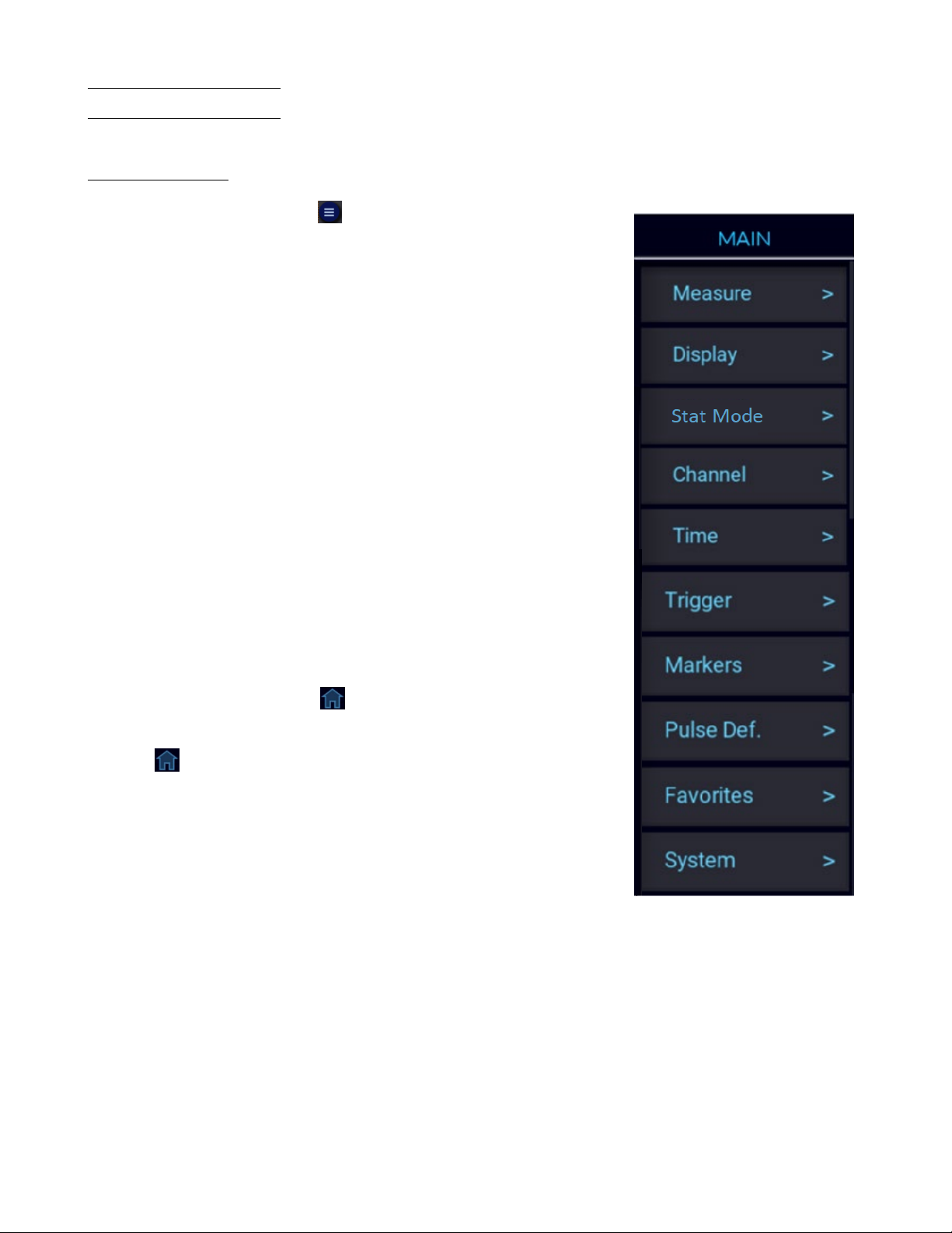
4.3.1 Main Menu
To open the Main menu press the icon.
The Main Menu shown in gure 4.2 is the top most menu level from which
all other menus originate.
Measure >
Display >
Stat. Mode >
Channel >
Time >
Trigger >
Markers >
Pulse Def. >
Favorites >
System >
When navigating any submenu the icon will appear to the right of the
submenu name.
Press the icon to return to the main menu.
Figure 4.2 Main Menu
Page 28

Operation 28
4.3.2 Measure >
To enter the Measure menu:
Press the icon then select the Measure menu.
The available setting vary depending on the mode selected. See gure 4.3 to view the available settings in each menu.
Measurement
Toogle the state of the data acquisition mode for taking measurements. If Measurement is set to Run, the RFM3000
immediately begins taking measurements (Continuous and Statistical modes), or arms its trigger and takes a measurement
each time a trigger occurs (Pulse Mode). If set to Stop, the measurement will begin (or be armed) if Start is selected
under the Single Sweep setting (Pulse Mode Only), and will stop once the measurement criteria (averaging) has been
satised.
Meas. Clear/Stat Capture
Selecting Execute clears display traces, data buers, and clears averaging lters to empty. In Statistical Measure mode,
the menu item is replaced with Stat Capture and selecting Reset clears the acquired sample population.
Single Sweep
Only available in Pulse mode. Select to start a single measurement cycle in Pulse mode when Measurement is set to
Stop. Enough trace sweeps must be triggered to satisfy the channel averaging setting.
Meas. Settings
This will load the default operating parameters listed in table 3.1. Only the settings shown in the table are aected and
all others remain in their current state.
Cont. Mode
Measure Menu
Pulse Mode
Measure Menu
Figure 4.3 Measure Menus
Stat. Mode
Measure Menu
Page 29
Operation 29
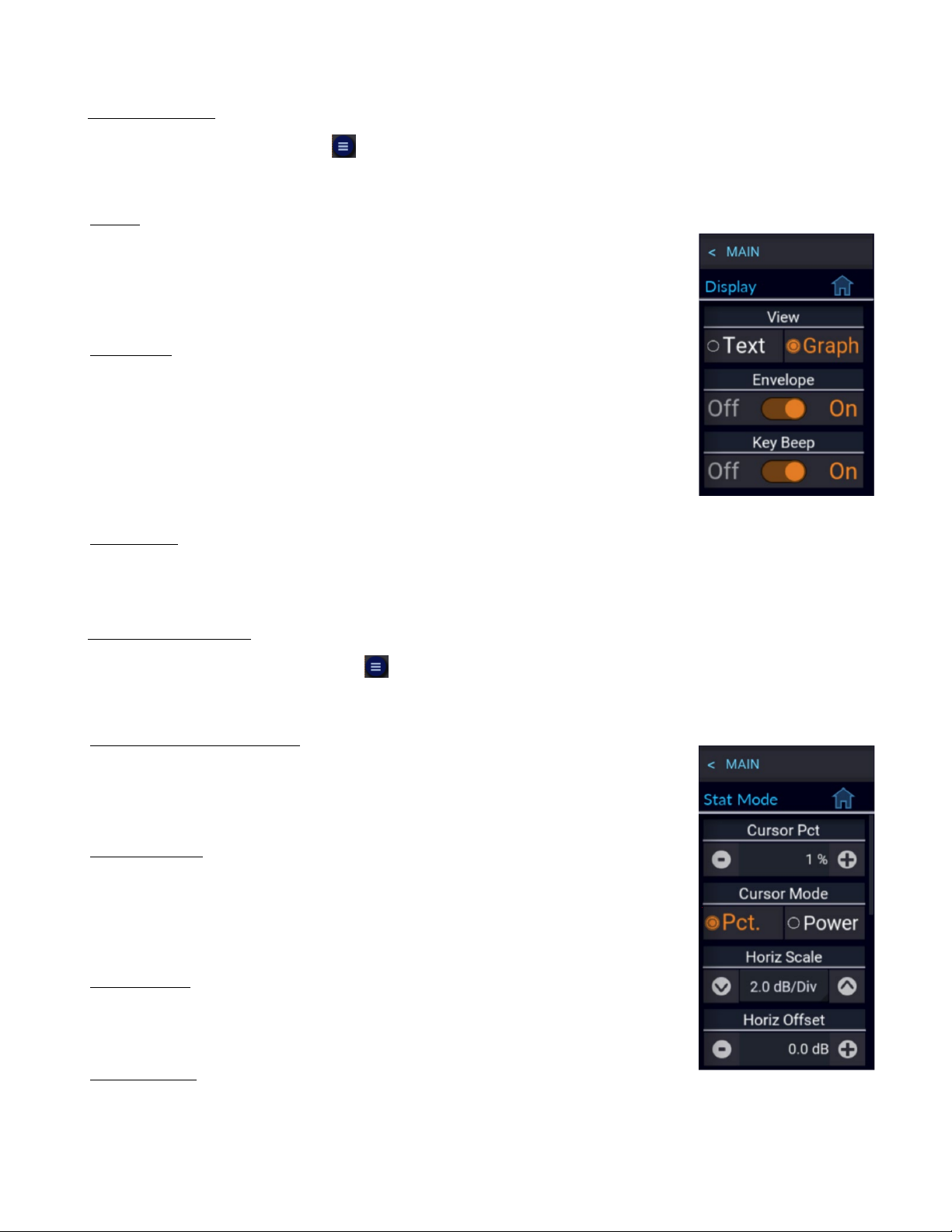
4.3.3 Display >
To enter the Display menu press the icon then select the Display menu.
View
Toogle between Text and Graph view. Text view displays a table of measurements for
the current measurement mode. In Continuous mode, selecting Text displays the enabled
channel power as shown in gure 3.1. Selecting Graph displays the trace graphical view.
Envelope
Enables/disables the Envelope display mode. In Pulse and Modulated modes, the Envelope display is used to highlight the range of signal excursions. When Envelope display
mode is On, the trace is drawn as a wide line. The line is lled in between the minimum
and maximum power readings. A series of vertical pixels, representing the range of signal
excursions or "envelope" of the signal will be illuminated for each horizontal trace pixel.
Envelope display is only available for Peak Power sensors.
Key Beep
Enable/disable the audible key beep.
4.3.4 Stat. Mode >
To enter the Stat. Mode menu press the icon then select the Stat. Mode menu.
Cursor Pct./Cur Pow Ref
Sets the CCDF cursor to the desired probability. When Cursor mode is set to Power, the
menu item changes to Cur Pow Ref and sets the desired power
Cursor Mode
Select the independent variable for the CCDF cursor. If Percent is selected, probability
at the cursor’s intersection with the CCDF curve will be measured. If Power is selected,
relative power at the cursor’s intersection with the CCDF curve will be measured.
Figure 4.4 Display Menu
Horiz Scale
Select the horizontal scale for the statistical graphic display.
Horiz Oset
Select the horizontal oset for statistical graphic display.
Figure 4.5 Stat. Mode
Page 30
Operation 30
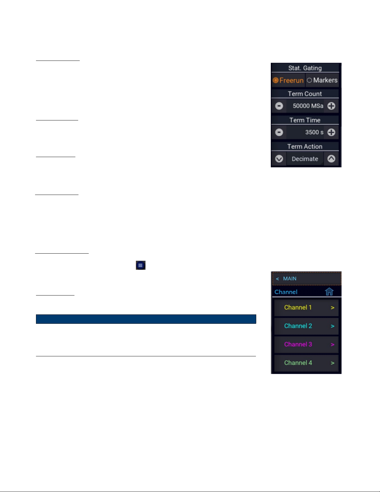
Stat. Gating
Select Freerun or Markers gating for statistical acquisition. If Freerun is selected, all
the samples are acquired without regard of sweep acquisition. If Markers are selected,
then only samples within the time marker interval on the Pulse mode triggered sweep
will be included in the statistical sample population.
Term Count
Sets the terminal sample count for the CCDF acquisition.
Term Time
Sets the terminal running time for the CCDF acquisition.
Figure 4.6 Stat. Mode
Term Action
Select the action to take when either the terminal count is reached or terminal time has elapsed. Selecting Decimate will
divide all sample bins by 2 and continue. The total sample count will be halved each time a decimation occurs. Selecting
Restart clears the statistical sample population and starts a new one. Selecting Stop will stop accumulating samples and
hold the result.
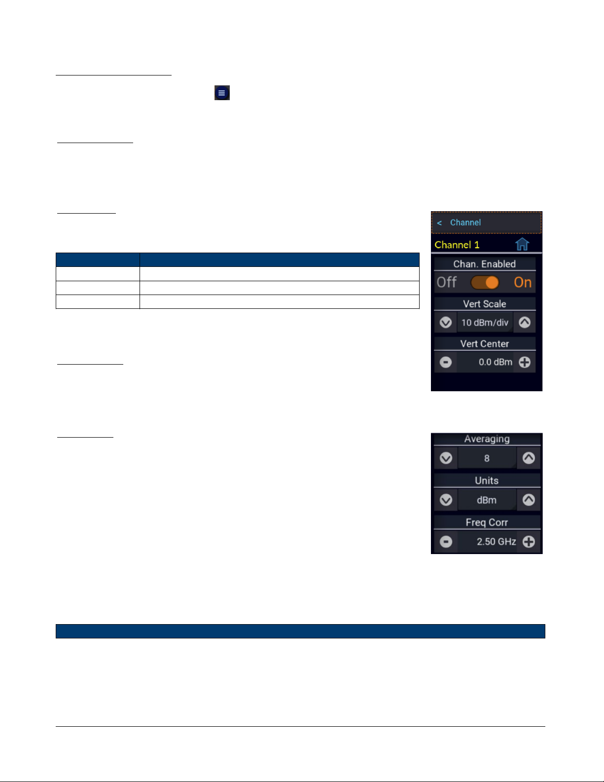
4.3.5 Channel >
To enter the Channel menu press the icon then select the Channel menu.
Channel #
Select the channels settings menu to be congured.
Note:
The base RFM3000 model only permits two sensors to be active at any one time.
With the RFM-4CH option, four sensors can be active at any one time.
Figure 4.7 Channels
Page 31
Operation 31
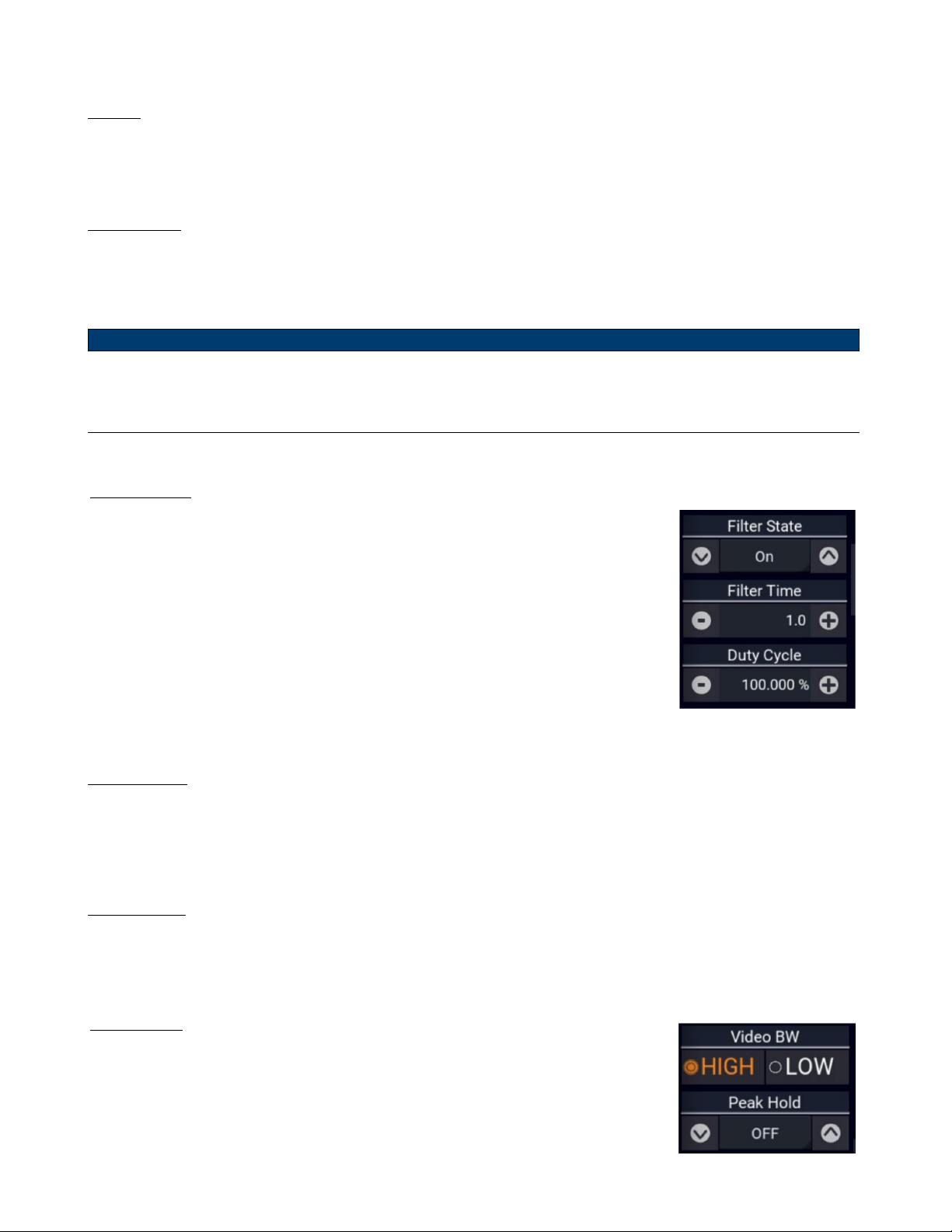
4.3.6 Channel Settings
To enter the Channel menu press the icon then select the Channel > Channel # menu.
Chan Enabled
Toggle the display of the trace and measurements for the selected channel. The channel may still be used as a trigger source when set to O.
Vert Scale
Set the power or voltage vertical axis level for the trace display based on the untis as
shown in table 4.8
Units Scale
dBm 0.1, 0.2, 0.5 1, 2, 5, 10, 20, 50 dB/div
Watts 1 pW to 500 MW/div in a 1-2-5 progression
Volts 1 µV to 100 kV/ div in a 1-2-5 progression
Table 4.1 Vertical Scale Range
Vert Center
Set the power or voltage, horizontal centerline, level of the graph for the specied
channel in the selected channel untis.
Averaging
Only available in Pulse and Statistical modes. Set the number of traces averaged together to form the measurement result on the selected channel. Averaging can be used
to reduce display noise on both the visible trace, marker, and automatic pulse measurements.
Trace averaging is a continuous process in which the measurement points from each
sweep are weighted (multiplied) by an appropriate factor and averaged into the existing
trace data points.
The most recent data will always have the greatest eect on the trace waveform, and
older measurements will be decayed at a rate determined by the averaging setting and
trigger rate. This averaging technique is often referred to as “exponential” averaging
because averaging imposes a rst-order Innite Impulse Response (IIR) exponential
lter with a time constant of "n" where n is the Average (number of averages) setting.
Note:
Figure 4.8
Channel Setttings
Figure 4.9
Channel Setttings
For timebase settings of 200 ns/div and faster, the RFP3000 Series sensors acquire samples using a technique called
equivalent time or random interleaved sampling (RIS). In this mode, not every pixel on the trace gets updated on
each sweep, and the total number of sweeps needed to satisfy the average setting will be increased by the sample interleave ratio of that particular timebase. At all times the average trace is the average of all samples for each pixel,
and the min/max are the lowest and highest of that same block of samples for each pixel.
Page 32
Operation 32
Units
Select the channel units. The trace may be shown in units of dBm, Watts, or Volts. The Units selection determines the
range of the scale values and also aects displayed text and measurement values.
Freq. Corr
Sets the measurement frequency for the RF signal that is applied to the sensor for the current measurement. The
appropriate frequency calibration factor from the sensor’s calibration table will be interpolated and applied automatically.
Application of this calibration factor compensates for the eect of variations in the atness of the sensor’s frequency
response.
Note:
The power sensor has no way to determine the carrier frequency of the applied signal, so the user must always enter
the frequency.
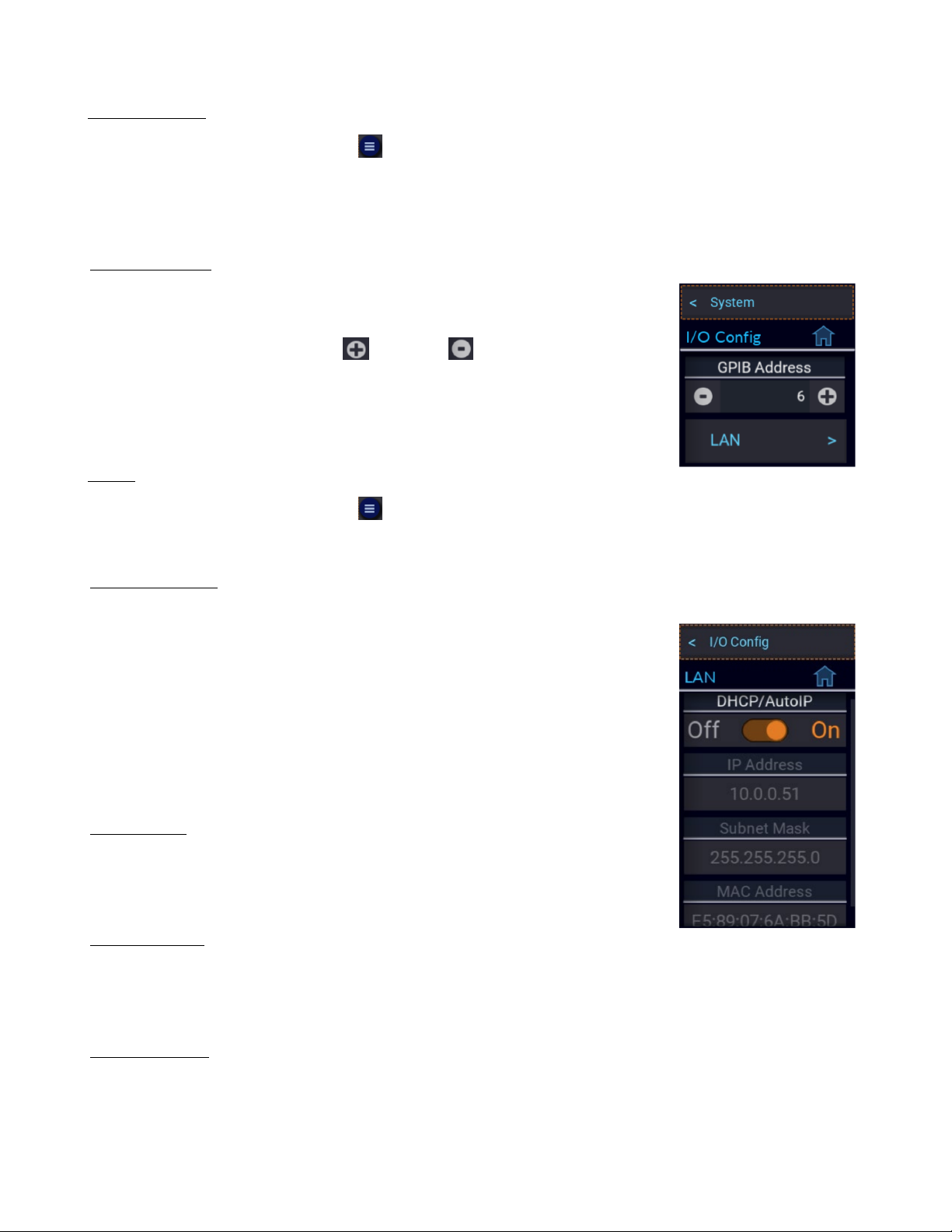
Filter State
Available in Continuous mode only. Sets the current value of the integration lter. The
lter can be set to O, On, or Auto.
O, provides no ltering, and can be used at high signal levels when absolute minimum
settling time is required.
On, allows a user-specied integration time to be entered for use.
Auto, uses a variable amount of ltering, which is set automatically by the power meter based on the current signal level to a value that gives a good compromise between
measurement noise and settling time at most levels.
Figure 4.10
Channel Setttings
Filter Time
Available in Continuous mode only. Sets the length of the integration lter. The lter is a “sliding window” which
averages samples taken within a time window whose duration is set by this eld. All samples within the time window are
equally weighted.
Duty Cycle
Available in Continuous mode only. Sets the duty cycle in percent for calculated CW pulse power measurements. Setting
the duty cycle to 100% is equivalent to a CW measurement.
Video BW
Sets the sensor video bandwidth of the selected channel. HIGH is appropriate for most
measurements. The actual bandwidth depends upon the sensor model.
LOW bandwidth oers additional noise reduction for CW or signals with very low
modulation bandwidth. If LOW bandwidth is used on signals with fast modulation,
measurement errors may result if the sensor cannot track the fast-changing envelope
of the signal.
Figure 4.11
Channel Setttings
Page 33

Operation 33
Peak Hold
Set the operating mode of the selected channel’s peak hold function.
When set to OFF, peak values are not held.
When set to instantaneous (INST) instantaneous peak readings are held until reset by a new acquisition or cleared
manually. This setting is used when it is desirable to hold the highest peak over a long measurement interval without
any decay.
When set to average (AVG) peak readings are held for a short time, and then decayed towards the average power at a rate
proportional to the Averaging setting. This is the best setting for most signals, because the peak will always represent
the peak power of the current signal, and the resulting peak-to-average ratio will be correct shortly after any signal level
changes.
dB Oset
Sets a measurement oset in dB for the selected channel. This is used to compensate for external couplers, attenuators, or ampliers in the RF signal path ahead of the
power sensor.
Zero
Performs a zero oset null adjustment. The sensor does not need to be connected to
any calibrator for zeroing. This action removes the eect of small, residual power osets, and should be performed prior to low-level measurements. The procedure is often
performed in-system. There should be no RF signal applied to the sensor input prior to
zeroing.
Figure 4.12
Channel Setttings
Fixed Cal
Performs a single point sensor gain calibration of the selected channel at 0 dBm and the current frequency setting. This
requires a calibrated 0 dBm (1.00 mW) signal source at the current measurement frequency. This procedure calibrates
the sensor’s gain at a single point. At other levels, that gain setting is combined with stored linearity factors to compute
the actual power.
The built-in test source of the RFM3000 is not a suciently calibrated source for performing
a xed calibration. An external calibration source is required. Note that xed calibration is
NOT REQUIRED for USB power sensors.
Page 34

Operation 34
4.3.7 Time >
To enter the Time menu press the icon then select the Time tab.
Timebase
Controls the timebase, horizontal scale, of the Trace View. The Timebase pulldown
menu permits selection of xed timebase ranges from 5 ns/div to 50 ms/div (sensor
series dependent) in a 1-2-5 progression.
Position
Sets the location of the trigger point on the acquired trace waveform. The Trig Delay
setting is in addition to this setting, and will cause the trigger position to appear in a
dierent location.
Figure 4.13
Time Setttings
Trig Delay
The trigger delay time is set in seconds with respect to the trigger. Positive values means that the trace display shows a
time interval after the trigger event. This positions the trigger event to the left of the trigger point on the display, and
is useful for viewing events during a pulse, or some xed delay time after the rising edge trigger. Negative trigger delay
mean that the trace display shows a time interval before the trigger event, and is useful for looking at events preceding
the trigger edge.
4.3.8 Trigger >
To enter the Trigger menu press the icon then select the Trigger tab.
Trigger Holdo
Set the trigger holdo time. Trigger holdo is used to disable the trigger for a specied amount of time after each trigger event. The holdo time starts immediately
after each valid trigger edge and will not permit any new triggers until the time has
expired. When the holdo time is up, the trigger re-arms, and the next valid trigger event (edge) will cause a new sweep. This feature is used to help synchronize the
power meter with burst waveforms such as a TDMA or GSM frame. The trigger holdo resolution is 0.01 microseconds, and it should be set to a time that is longer than
the burst duration but shorter than the frame repetition interval.
Trigger Level
Sets the threshold level for the trigger signal used in the Auto and Normal trigger
modes. The trigger level can be entered numerically or changed by using arrow keys.
The trigger level range has a range that is sensor model dependent (see the sensor
specications for your specic sensor model).
The trigger range is automatically adjusted to include the dB Oset parameter set for the
source channel. For example, if the trigger level = 10 dBm and the dB Oset is changed
Figure 4.14
Trigger Setttings
Page 35

Operation 35
from 0 to 20 dB, then the oset-adjusted trigger level will be displayed to the user as 30 dBm. Likewise, the maximum
trigger level range will be extended to 40 dBm. The trigger level set point and setting range are both shifted upward by
20 dB.
Trigger Mode
Set the trigger mode for synchronizing data acquisition with pulsed signals.
Normal mode will cause a sweep to be triggered each time the power level crosses the preset trigger level in the direction
specied by the trigger slope setting. If there are no edges that cross this level, no data acquisition will occur.
Auto mode operates in much the same way as Normal mode but will automatically generate a trace if no trigger edges
are detected for a period of time (100 to 500 milliseconds, depending upon timebase). This will keep the trace updating
even if the pulse edges stop.
The Auto PK-PK mode operates the same as Auto mode but will adjust the trigger level to halfway between the highest
and lowest power or voltage levels detected. This aids in maintaining synchronization with a pulse signal of varying level.
The Freerun mode forces unsynchronized traces at a high rate to assist in locating the signal.
Trigger Source
Set the trigger source used for synchronizing data acquisition. The CH # settings use the signal from the associated
sensor. Ext setting uses the signal applied to the rear panel TRIG IN connector.
The trigger source can be any of the resource channels (CH1, CH2, etc.), or the Ext(ernal) trigger input signal. The
Ind(ependent) trigger setting allows each connected sensor to trigger independently from its own RF input.
The external trigger is attached to the Trig In BNC connector on the rear of the RFM3000 Power Meter and requires a
TTL signal level, minimum pulse width of 10 ns, and maximum frequency of 50 MHz.
Note:
Connecting the Sync cable from the Multi I/O port on the sensor to the corresponding Sync port on the instrument
for the sensor in use is necessary if using an external trigger or when performing measurements across multiple channels.
Trigger Slope
Set the trigger slope or polarity. When set to +, trigger events will be generated when a signal’s rising edge crosses the
trigger level threshold. When – is selected, trigger events are generated on the falling edge of the pulse.
Page 36

Operation 36
Markers >
To enter the Markers menu press the icon then select the Markers > tab.
Marker #
Set the time position of marker 1 or 2 relative to the trigger. Note that time markers
must be positioned within the time limits of the trace window in the graph display. If
a time outside of the display limits is entered, the marker will be placed at the rst or
last time position as appropriate.
ΔTime
Displays the result of Marker 2 - 1 in seconds. This item is read only.
Figure 4.15
Marker Setttings
4.3.9 Pulse Def. >
To enter the Pulse Def menu press the icon then select the Pusle Def. > tab.
CH # Pulse Def
Select the channel to be congured.
Figure 4.16
Pulse Def Menu
4.3.10 CH# Pulse Def
To enter the CH# Pulse Def menu press the icon then select the CH# Pusle Def. > tab of the channel to be
congured.
Page 37

Operation 37
Distal
Sets the pulse amplitude percentage that denes the end of a rising edge or beginning
of a falling edge transition. Typically, this is 90% voltage or 81% power relative to the
top level of the pulse. This setting is used when making automatic pulse risetime and
falltime calculations.
Mesial
Sets the pulse amplitude percentage that denes the midpoint of a rising or falling
edge transition. Typically, this is 50% voltage or 25% power relative to the top level
of the pulse. This setting is used when making automatic pulse width and duty cycle
calculations.
Proximal
Sets the pulse amplitude percentage that denes the beginning of a rising edge or end
of a falling edge transition. Typically, this is 10% voltage or 1% power relative to the
top level of the pulse. This setting is used when making automatic pulse risetime and
falltime calculations.
Pulse Unites
Controls whether the distal, mesial, and proximal thresholds are computed as voltage or
power percentages of the top/bottom amplitudes. If Volts is selected, the pulse transition thresholds are computed as voltage percentages. If Watts are selected, they are
computed as power percentages.
units setting.
Many pulse measurements call for 10% to 90% voltage (which equates to 1% to 81% power) for risetime and falltime
measurements, and measure pulse widths from the half-power (–3 dB, 50% power, or 71% voltage) points. The Pulse
Units setting is independent of the channel’s display
Figure 4.17
CH# Pulse Def Menu
Start Gate
Sets the beginning of the pulse measurement region as a percentage of the pulse width. The Start Gate has a continuous
range of 0.0% to 40.0% of the pulse width and may be entered numerically or varied using the up or down arrows.
End Gate
Sets the end of the pulse measurement region as a percentage of the pulse width. The End Gate has a continuous range
of 60.0% to 100.0% of the pulse width and may be entered numerically or varied using the up or down arrows.
The Gate settings dene the measurement interval for the following power related pulse measurements: Pulse Average,
Pulse Peak, Pulse Minimum, and Pulse Droop/Tilt. Pulse timing measurements between mesial crossings such as width
and period are not aected. The purpose of the Pulse Gate setting is to exclude edge transition eects from the pulse
power measurements.
Page 38

Operation 38
4.3.11 Favorites >
To enter the Favorites menu press the icon then select the Favorites > tab.
This function is not fully implemented at this time). Enables the user to setup a customized menu to allow grouping
frequently used menu items into one convenient menu.
4.3.12 System >
To enter the System menu press the icon then select the System > tab.
The System menu displays the available system-level features and functionality.
Seonsr Data >
I/O Cong >
Calibration >
Exit >
Reports >
Update Software
cm
Figure 4.18 System Menu
Sensor Data >
To enter the Sensor Data menu press the icon then select the System > Sensor Data > tab.
Press Show to display information about the selected sensor in a pop-up log.
See gure 4.19.
Figure 4.19 CH1 Information
Figure 4.20 Sensor Data
Page 39
Operation 39
I/O Cong >
To enter the I/O Cong menu press the icon then select the System > I/O Cong > tab.
The RFM3000 supports remote communication over LAN and GPIB (optional).
GPIB Address
Set and View the current GPIB address in use for instruments equipped with GPIB
option.
To increae the GPIB address press the icon or the icon do decrease the address. Pressing the number box located between the increase and decrease icon will
open the numeric keypad. The numeric keypad can be used to instantaneously change
the GPIB address
LAN
Figure 4.21 I/O Cong
To enter the I/O Cong menu press the icon then select the System > I/O Cong > LAN > tab.
DHCP/AutoIP
Set the state of DHCP/AutoIP system for the Ethernet port.
If DHCP/AutoIP is enabled (On), the instrument will attempt to obtain its IP Address
and Subnet Mask, a DHCP (dynamic host conguration protocol) server on the network. If no DHCP server is found, the instrument will select its own IP Address and
Subnet Mask values using the AutoIP protocol.
If DHCP/AutoIP is disabled (O), the instrument will use the IP Address and Subnet
Mask values that have been set by the user.
IP Address
Set the Internet Protocol (IP) address of the Ethernet adapter. If DHCP/AutoIP mode
is enabled, this menu is read-only.
Subnet Mask
Figure 4.22 LAN
Set the subnet mask for the Ethernet adapter. If DHCP/AutoIP mode is enabled, this
menu is read-only.
MAC Address
Displays the MAC address for the Ethernet adapter. This menu item is read-only.
Page 40

Operation 40
Calibration >
To enter the Calibrator menu press the icon then select the System > Calibrator > tab.
Cal Output
Enable/disable the output of the built-in 0 dBm 50 MHz test source.
Note:
The built-in test source of the RFM3000 is not a suciently calibrated source for performing a xed calibration. An external calibration source is required.
Figure 4.23 Calibrator
Exit >
To enter the Exit menu press the icon then select the System > Exit > tab.
Exit to Desktop
Exits the RFM3000 Power Meter Main application to access the OS Desktop.
Shut Down
Shuts down power to the PMX40 putting the meter in standby mode and is the same
as pressing the ON/Standby button on the front panel.
Reports >
To enter the Reports menu press the icon then select the System > Reports > tab.
Conguration
Select Show to display an About dialog with conguration information for the
RFM3000 Power Meter like that shown in gure 2.2.
Figure 4.24 Exit
Figure 4.25 Reports
Page 41
Operation 41
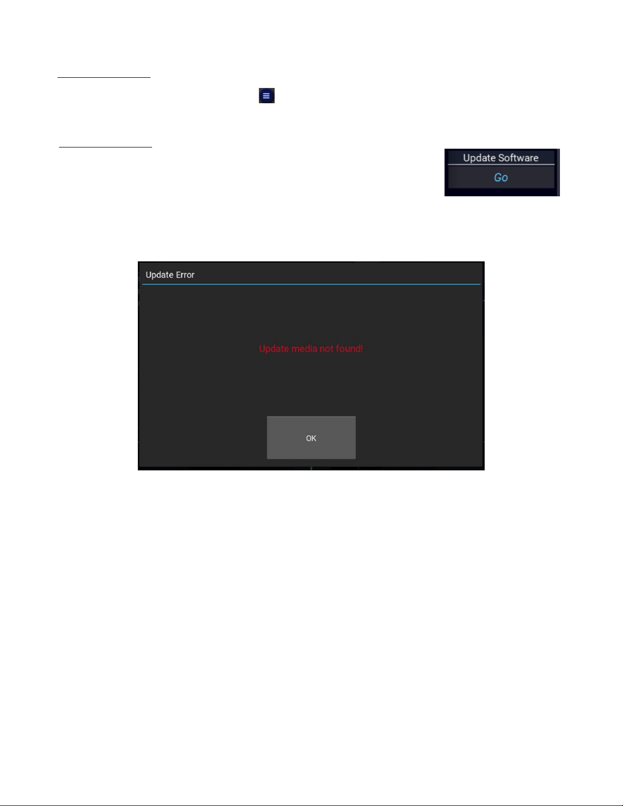
Update Software
To view the Update Sofware option press the icon then select the System > tab.
Update Software
Select Go to search the connected USB drive for the *.tar software update le and update or re-install the version found. If no valid le is found, the dialog in gure 4.27
appears.
Figure 4.26
Update Software
Figure 4.27 Update Error
Page 42

Application Notes
This section provides supplementary material to enhance your knowledge of the RFM3000 operation, advanced features, and measurement accuracy. Topics covered in this section include pulse measurement fundamentals, automatic
measurement principles, and an analysis of measurement accuracy.
5.1 Introduction to Pulse Measurements
5.1.1 Measurement Fundamentals
The following is a brief reaview of the power measurement fundamentals.
Unmodulated Carrier Power
The average power of an unmodulated carrier consisting of a continuous, constant amplitude sinewave signal is also
termed continuous wave (CW) power. For a known value of load impedance R, and applied voltage 𝑉
power is:
2
𝑉
𝑟𝑚𝑠
𝑃 =
𝑅
𝑤𝑎𝑡𝑡𝑠
, the average
𝑟𝑚𝑠
Power meters designed to measure CW power can use thermoelectric-based sensors which respond to the heating eect of
the signal or diode detectors which respond to the voltage of the signal. With careful calibration accurate measurements
can be obtained over a wide range of input power levels.
Modulated Carrier Power
The average power of a modulated carrier which has varying amplitude can be measured accurately by a CW type power
meter with a thermoelectric detector, but the lack of sensitivity will limit the range. Diode detectors can be used at low
power, square-law response levels. At higher power levels the diode responds in a more linear manner and signicant
error results.
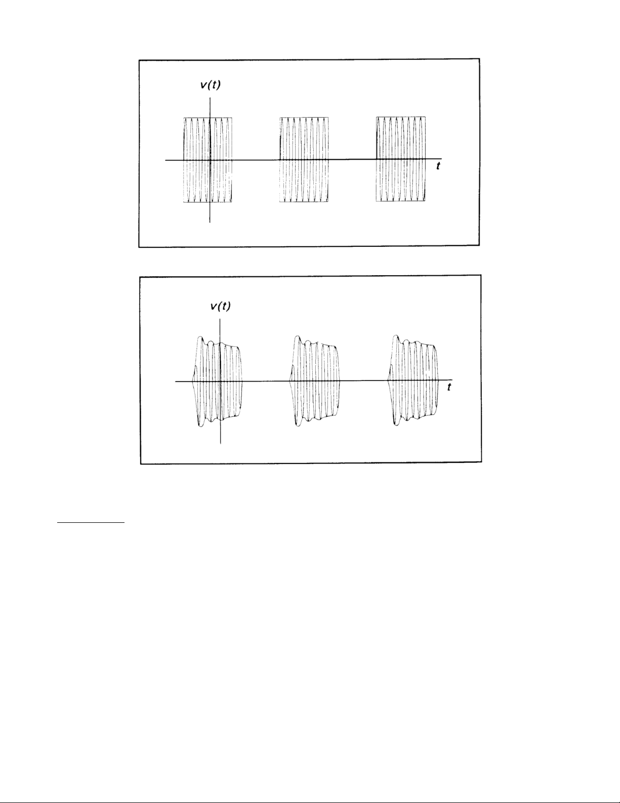
Pulse Power
Pulse power refers to power measured during the on time of pulsed RF signals gure 5.1. Traditionally, these signals
have been measured in two steps: (1) thermoelectric sensors measure the average signal power, (2) the reading is then
divided by the duty cycle to obtain pulse power, 𝑃
𝑃
Where Duty Cycle:
𝐷𝑢𝑡𝑦 𝐶𝑦𝑐𝑙𝑒 =
𝑝𝑢𝑙𝑠𝑒
𝑝𝑢𝑙𝑠𝑒
:
𝐴𝑣𝑒𝑟𝑎𝑔𝑒 𝑃 𝑜𝑤𝑒𝑟
=
𝐷𝑢𝑡𝑦 𝐶𝑦𝑐𝑙𝑒
𝑃𝑢𝑙𝑠𝑒 𝑊𝑖𝑑𝑡ℎ
𝑃𝑢𝑙𝑠𝑒 𝑃 𝑒𝑟𝑖𝑜𝑑
Pulse power provides useful results when applied to rectangular pulses, but is inaccurate for pulse shapes that include
distortions, such as overshoot or droop (Figure 5.2).
Page 43
Application Notes 43
Figure 5.1 Pulsed RF Signal
Figure 5.2 Distorted Pulsed Signal
Peak Power
The RFM3000 makes power measurements in a manner that overcomes the limitations of the pulse power method and
provides both peak power and average power readings for all types of modulated carriers. The fast-responding diode
sensors detect the RF signal to produce a wideband video signal, which is sampled with a narrow sampling gate. The
video sample levels are accurately converted to power on an individual basis at up to a 100 MSa/sec rate. Since this
power conversion is corrected based upon the sensor’s linearity correction table, these samples can be averaged to yield
average power without restriction to the diode square-law region.
If the signal is repetitive, the signal envelope can be reconstructed using an internal or external trigger. The envelope
can be analyzed to obtain waveshape parameters including, pulse width, duty cycle, overshoot, rise time, fall time, and
droop. In addition to time domain measurements and simple averaging, the RFM3000 has additional capabilities that
allow it to perform statistical analysis on a complete set of continuously sampled data points.
Data can be viewed and characterized using a CCDF presentation format. These analysis tools provide invaluable
information about peak power levels and their frequency of occurrence, and are especially useful for non-repetitive
signals, such as those used in 5G and Wi-Fi applications.
Page 44

Application Notes 44
5.1.2 Diode Detection
Wideband diode detectors are the dominant power sensing device used to measure pulsed RF signals. Several diode
characteristics must be compensated to make meaningful measurements. These include the detector’s nonlinear amplitude response, temperature sensitivity, and frequency response characteristic. Additional potential error sources include
detector mismatch, signal harmonics, and noise.
Detector Response
The response of a single-diode detector to a sinusoidal input is given by the diode equation:
𝑖 = 𝐼𝑠(𝑒𝑎𝑣− 1)
where:
𝑖 = 𝑑𝑖𝑜𝑑𝑒𝑐𝑢𝑟𝑟𝑒𝑛𝑡
𝑣 = 𝑛𝑒𝑡𝑣𝑜𝑙𝑡𝑎𝑔𝑒𝑎𝑐𝑟𝑜𝑠𝑠𝑡ℎ𝑒𝑑𝑖𝑜𝑑𝑒
𝐼𝑠= 𝑠𝑎𝑡𝑢𝑟𝑎𝑡𝑖𝑜𝑛𝑐𝑢𝑟𝑟𝑒𝑛𝑡
𝛼 = 𝑐𝑜𝑛𝑠𝑡𝑎𝑛𝑡
An ideal diode response curve is plotted in gure 5.3
Figure 5.3 Ideal Diode Response
The curve indicates that for low microwave input levels (Region A), the single-diode detector output is proportional to
the square of the input power. For high input signal levels (Region C), the output is linearly proportional to the input.
In between these ranges (Region B), the detector response lies between square-law and linear.
For accurate power measurements over all three regions illustrated in gure 5.3, the detector response is pre-calibrated
over the entire range. The calibration data is stored in the instrument and recalled to adjust each sample of the pulse
power measurement.
Page 45

Application Notes 45
Temperature Eects
The sensitivity of microwave diode detectors (normally Low Barrier Schottky diodes) varies with temperature. However,
ordinary circuit design procedures that compensate for temperature-induced errors adversely aect detector bandwidth.
A more eective approach involves sensing the ambient temperature during calibration and recalibrating the sensor when
the temperature drifts outside the calibrated range.
This process can be made automatic by collecting calibration data over a wide temperature range and saving the data in
a form that can be used by the power meter to correct readings for ambient temperature changes.
Frequency Response
The carrier frequency response of a diode detector is determined mostly by the diode junction capacitance and the device
lead inductances.
The frequency response will vary from detector to detector and cannot be compensated readily. Power measurements
must be corrected by constructing a frequency response calibration table for each detector.
Mismatch
Sensor impedance matching errors can contribute signicantly to measurement uncertainty, depending on the mismatch
between the device under test (DUT) and the sensor input. This error cannot be easily calibrated out, but can be
minimized by employing an optimum matching circuit at the sensor input.
Signal Harmonics
Measurement errors resulting from harmonics of the carrier frequency are leveldependent and cannot be calibrated out.
In the square-law region of the detector response (Region A, Figure 5-3), the signal and second harmonic combine on
a root mean square basis. The eects of harmonics on measurement accuracy in this region are relatively insignicant.
However, in the linear region (Region C, gure 5.3), the detector responds to the vector sum of the signal and harmonics.
Depending on the relative amplitude and phase relationships between the harmonics and the fundamental, measurement
accuracy may be signicantly degraded. Errors caused by even-order harmonics can be reduced by using balanced diode
detectors for the power sensor. This design responds to the peak-to-peak amplitude of the signal, which remains constant
for any phase relationship between fundamental and even-order harmonics. Unfortunately, for odd-order harmonics, the
peak-to-peak signal amplitude is sensitive to phasing, and balanced detectors provide no harmonic error improvement.
Measurement errors resulting from harmonics of the carrier frequency are leveldependent and cannot be calibrated out.
In the square-law region of the detector response (Region A, gure 5.3), the signal and second harmonic combine on
a root mean square basis. The eects of harmonics on measurement accuracy in this region are relatively insignicant.
However, in the linear region (Region C, gure 5.3), the detector responds to the vector sum of the signal and harmonics.
Depending on the relative amplitude and phase relationships between the harmonics and the fundamental, measurement
accuracy may be signicantly degraded. Errors caused by even-order harmonics can be reduced by using balanced diode
detectors for the power sensor. This design responds to the peak-to-peak amplitude of the signal, which remains constant
for any phase relationship between fundamental and even-order harmonics. Unfortunately, for odd-order harmonics, the
peak-to-peak signal amplitude is sensitive to phasing, and balanced detectors provide no harmonic error improvement.
Noise
For low-level signals, detector noise contributes to measurement uncertainty and cannot be calibrated out. Balanced
detector sensors improve the signal-to-noise ratio by 3 dB, because the signal is twice as large.
Page 46

Application Notes 46
5.1.3 Pulse Denitions
IEEE Std 194™-1977 Standard Pulse Terms and Denitions “provides fundamental denitions for general use in time
domain pulse technology.” Several key terms dened in the standard are reproduced in this subsection, which also denes
the terms appearing in the RFM3000 text mode display of automatic measurement results.
5.1.4 Standard IEEE Pulse
The key terms dened by the IEEE standard are abstracted and summarized below. These terms are referenced to the
standard pulse illustrated ingure 5.4
Figure 5.4 Stanard IEEE Pulse
Note:
IEEE Std 194™-1977 Standard Pulse Terms and Denitions has been superseded by IEEE Std 181™-2003. Many of
the terms used below have been deprecated by the IEEE. However, these terms are widely used in the industry. For
this reason, they are retained.
Page 47

Application Notes 47
Term Denition
Base Line
Top Line The portion of a pulse waveform which represents the second nominal state of a pulse.
First Transition
Last Transition
Proximal Line
Distal Line
Mesial Line
The two portions of a pulse waveform which represent the rst nominal state from
which a pulse departs and to which it ultimately returns.
The major transition of a pulse waveform between the base line and the top line (commonly called the rising edge).
The major transition of a pulse waveform between the top of the pulse and the base
line (commonly called the falling edge).
A magnitude reference line located near the base of a pulse at a specied percentage
(normally 10%) of pulse magnitude.
A magnitude reference line located near the top of a pulse at a specied percentage
(normally 90%) of pulse magnitude.
A magnitude reference line located in the middle of a pulse at a specied percentage
(normally 50%) of pulse magnitude.
Table 5.1 Pule Terms
5.1.5 Automatic Measurements
The RFM3000 automatically analyzes the waveform data in the buers and calculates key waveform parameters. The
calculated values are displayed in text mode when you press the TEXT/GRAPH system key.
5.1.6 Automatic Measurement Criteria
Automatic measurements are made on repetitive signals that meet the following conditions:
• Amplitude
– The dierence between the top and bottom signal amplitudes must exceed 6 dB to calculate waveform timing
parameters (pulse width, period, duty cycle). The top-to-bottom amplitude dierence must exceed 13 dB to
measure rise and fall time.
• Timing
To measure pulse repetition frequency and duty cycle, there must be at least three signal transitions. The interval
between the rst and third transition must be at least 1/5 of a division (1/50 of the screen width). For best
accuracy on rise and fall time measurements, the timebase should be set so the transition interval is at least
one-half division on the display.
Page 48

Application Notes 48
5.1.7 Automatic Measurement Terms
The following terms appear in the RFM3000 Text display in Pulse mode. The Text column lists the abbreviated forms
that appear on the display screen.
Text TERM DEFINITION
Width Pulse Width The interval between the rst and second signal crossings of the mesial line.
Rise Risetime The interval between the rst signal crossing of the proximal line to the rst
signal crossing of the distal line.
Fall Falltime The interval between the last signal crossing of the distal line to the last signal
crossing of the proximal line.
Period Pulse Period The interval between two successive pulses (reciprocal of the Pulse Repetition
Frequency).
PRFreq Pulse Repetition The number of cycles of a repetitive signal that take place in one Frequency
second.
Duty C Duty Cycle The ratio of the pulse on-time to o-time. Otime O-time The time a repeti-
tive pulse is o (equal to the pulse period minus the pulse width).
Peak Peak Power The maximum power level of the captured waveform.
Pulse Pulse Power The average power level across the pulse width, dened by the intersection of
the pulse rising and falling edges with the mesial line.
Avg Average Power The equivalent heating eect of a signal. IEEETop Top Amplitude The ampli-
tude of the top line (see IEEE denitions). IEEEBot Bottom Amplitude The
amplitude of the base line (see IEEE denitions). Skew Skew The time between
the mesial level of a pulse on one channel and a pulse on a second channel.
EdgeDly Edge Delay The time between the left edge of the display and the rst mesial transition level
of either slope on the waveform.
Table 5.2 Automatic Measurement Terms
Page 49

Application Notes 49
5.1.8 Automatic Measurement Sequence
The automatic measurement process analyzes the captured signal data in the following sequence:
1. Approximately 500 samples of the waveform (equivalent to one screen width) are scanned to determine the maximum
and minimum sample amplitudes.
2. The dierence between the maximum and minimum sample values is calculated and stored as the Signal Amplitude.
3. The Transition Threshold is computed as one-half the sum of the maximum and minimum sample amplitudes.
4. The processor locates each crossing of the Transition Threshold.
5. Starting at the left edge of the screen, the processor classies each Transition threshold crossing according to whether
it is positive-going (– +) or negative-going (+ –). Because the signal is repetitive, only three transitions are needed
to classify the waveform, as follows:
Type Sequence Description
0 none No crossings detected
1 Not used
2 + – One falling edge
3 – + One rising edge
4 + – + One falling, followed by one rising edge
5 – + – One rising, followed by one falling edge
6 + – + – Two falling edges
7 – + – + Two rising edges
Table 5.3 Transition Threshold Crossing
Figure 5.5 Step Waveforms
Page 50

Application Notes 50
6. If the signal is Type 0, (No crossings detected) no measurements can be performed and the routine is terminated,
pending the next reload of the data buers.
7. The process locates the bottom amplitude (baseline) using the IEEE histogram method. A histogram is generated
for all samples in the lowest 12.8 dB range of sample values. The range is subdivided into 64 power levels of 0.2
dB each. The histogram is scanned to locate the power level with the maximum number of crossings. This level is
designated the baseline amplitude. If two or more power value have equal counts, the lowest is selected.
8. The process follows a similar procedure to locate the top amplitude (top line). The power range for the top histogram
is 5 dB and the resolution is 0.02 dB, resulting in 250 levels. The level-crossing histogram is computed for a single
pulse, using the samples which exceed the transition threshold. If only one transition exists in the buer (Types 2
and 3), the process uses the samples that lie between the edge of the screen and the transition threshold (see gure
5.6). For a level to be designated the top amplitude, the number of crossings of that level must be at least 1/16 the
number of pixels in the pulse width; otherwise, the peak value is designated the top amplitude.
Figure 5.6 Time Interpolation
9. The process establishes the proximal, mesial, and distal levels as a percentage of the dierence between top amplitude
and bottom amplitude power. The percentage can be calculated on a power or voltage basis. The proximal, mesial,
and distal threshold values are user settable from 1% to 99%, with the restriction that the proximal < mesial < distal.
Normally, these values will be set to 10%, 50%, and 90%, respectively.
10. The process determines horizontal position, in pixels, at which the signal crosses the mesial value. This is done to
a resolution of 0.1 pixel, or 1/5000 of the screen width. Ordinarily, the sample values do not fall precisely on the
mesial line, and it is necessary to interpolate between the two nearest samples to determine where the mesial crossing
occurred. This process is demonstrated in the example above (gure 5.6):
Page 51

Application Notes 51
Item dBm mW
Mesial value 10.0 10.0
Sample n 8.0 6.3
Sample n+1 11.0 12.6
Table 5.4 Interpolation Crossing
The interpolated crossing time, 𝑡𝑥, is calculated from:
𝑡𝑥= 𝑡𝑛+
𝑚𝑒𝑠
𝑃
𝑛+1
− 𝑃
𝑛
𝑛
𝑃
− 𝑃
where 𝑃 is in watts and n is the number of the sampling interval, referenced to the trigger event.
For this example:
𝑡𝑥= 𝑡𝑛+
10.0 − 6.3
12.6 − 6.3
𝑡𝑥= 𝑡𝑛+ 0.6
11. The processor computes the rise and/or fall times of waveforms that meet the following conditions:
• The waveform must have at least one usable edge (Types 2 through 7).
• The signal peak must be at least 13 dB greater than the minimum sample value.
The rise time is dened as the time between the proximal and distal crossings (– +).
The fall time is dened as the time between the distal and proximal crossings (+ –).
If no samples lie between the proximal and distal values for either edge (rise or fall), the risetime for that edge is set
to 0 seconds.
12. The processor calculates the output values according to the following denitions:
a)
b)
c)
d)
e)
Pulse Width
Rise time
Fall time
Period Cycle
Pulse Repetition
Interval between mesial points
See Step 11
See Step 11
time between mesial points
Reciprocal of Period Frequency
f)
g)
h)
i)
j)
k)
l)
m)
n)
Duty Cycle Pulse
O-time
Peak Power
Pulse Power
Overshoot
Average Power
Top Amplitude
Bottom Amplitude
Skew
Pulse Width/Period
(Period) - (Pulse Width)
Maximum sample value (See Step 1)
Average power in the pulse (between the mesial points)
(Peak Power) - (Top Amplitude)
See Step 13
See Step 8
See Step 7
See Step 14
Page 52

Application Notes 52
5.1.9 Average Power Over an Interval
13. The average power of the signal over a time interval is computed by:
a)
b)
summing the sample powers in the interval
dividing the sum by the number of samples
This process calculates Pulse Power, Average Power, and the average power between markers.
Since each sample represents the power in a nite time interval, the endpoints are handled separately to avoid
spreading the interval by one-half pixel at each end of the interval (see gure ??). For the interval in gure ??, the
average power is given by:
𝑎𝑣𝑔
1
=
(𝑃0+ 𝑃𝑛) +
2
𝑃
1
𝑛 − 1
𝑛−1
∑
𝑛=1
𝑃
𝑛
Figure 5.7 Sampling Interval
14. The processor calculates the delay between the two measurement channels. The time reference for each channel is
established by the rst signal crossing (starting from the left edge of the screen) which passes through the mesial
level. The signal excursion must be at least 6 dB.
Page 53

Application Notes 53
5.1.10 Statistical Mode Automatic Measurements
When operating in Statistical mode, the RFM3000 has a unique text format display that is available when the TEXT/GRAPH
system key is pressed. A sample of the text display is shown in gure 5.8.
Figure 5.8 Statistical Mode Text Display
In the Statistical mode the following ve automatic measurements are displayed in the RFM3000 Text display for both
input channels and both trigger channels. The Text column lists the abbreviated forms that appear on the display screen.
In the Statistical mode the following ve automatic measurements are displayed in the PMX40 Text display for both
input channels and both trigger channels. The Text column lists the abbreviated forms that appear on the display screen.
TEXT TERM DEFINITION
Avg Average Power The unweighted average of all linear power samples occurring since acqui-
sition started.
Peak Peak Power The highest power sample occurring since acquisition was started.
Min Minimum Power The lowest power sample occurring since acquisition was started. In loga-
rithmic units a reading below the clip level will display as down arrows.
Pk2Avg Pk/Avg Ratio The ratio (in dB) of the Peak Power to the Average Power.
Table 5.5 Statistical Automatic Measurements
Page 54

Application Notes 54
The following six cursor measurements display the set position (independent variable) and measured value (dependent
variables) where the movable cursor intersects the measurement trace.
The position or value measurement text for each dependent variable is displayed in the color of its channel. The
independent variable is white.
Note that the intersection of the movable cursors and the CCDF traces can be moved outside the visible display area.
This does not aect the measurements in any way.
TEXT TERM DEFINITION
Cursor Pwr Cursor Powe Cursor Mode - Power Ref
Reference The reference power level in dBr set by the user to dene the measure-
ment point on the normalized CCDF for probability in percent.
Cursor Mode - Percent
The measured power level in dBr of the normalized CCDF at the Probability in percent specied by the user.
Cursor Pct Cursor Percentage Cursor Mode - Power Ref
The measured probability in percent of the normalized CCDF at the reference power level specied by the user.
Cursor Mode - Percent
The probability in percent set by the user to dene the measurement
point on the normalized CCDF for power level in dBr.
Total Time The total time in Hours:Minutes:Seconds that the data acquisition has
been running.
Points The total number of data samples in MSa that has been acquired for
each channel in the current run.
Table 5.6 Cursor Measurements
Note:
The total number of data samples is aected by the terminal settings. If Terminal Action is set to decimate, then
the sample count will be halved each time the Terminal Count or Time is reached. This should have very little visible
eect on the CCDF values, since the entire population is decimated uniformly. If Terminal Action is set to restart,
then the sample count will be cleared to zero each time the Terminal Count or Time is reached.
5.2 Measurement Accuracy
The measurement accuracy of the RFM3000 is completely contingent upon the USB sensor with which it is being used.
Please reference the sensor datasheet and/or associated uncertainty calculator for measurement uncertainties associated
with a specic sensor.
Page 55
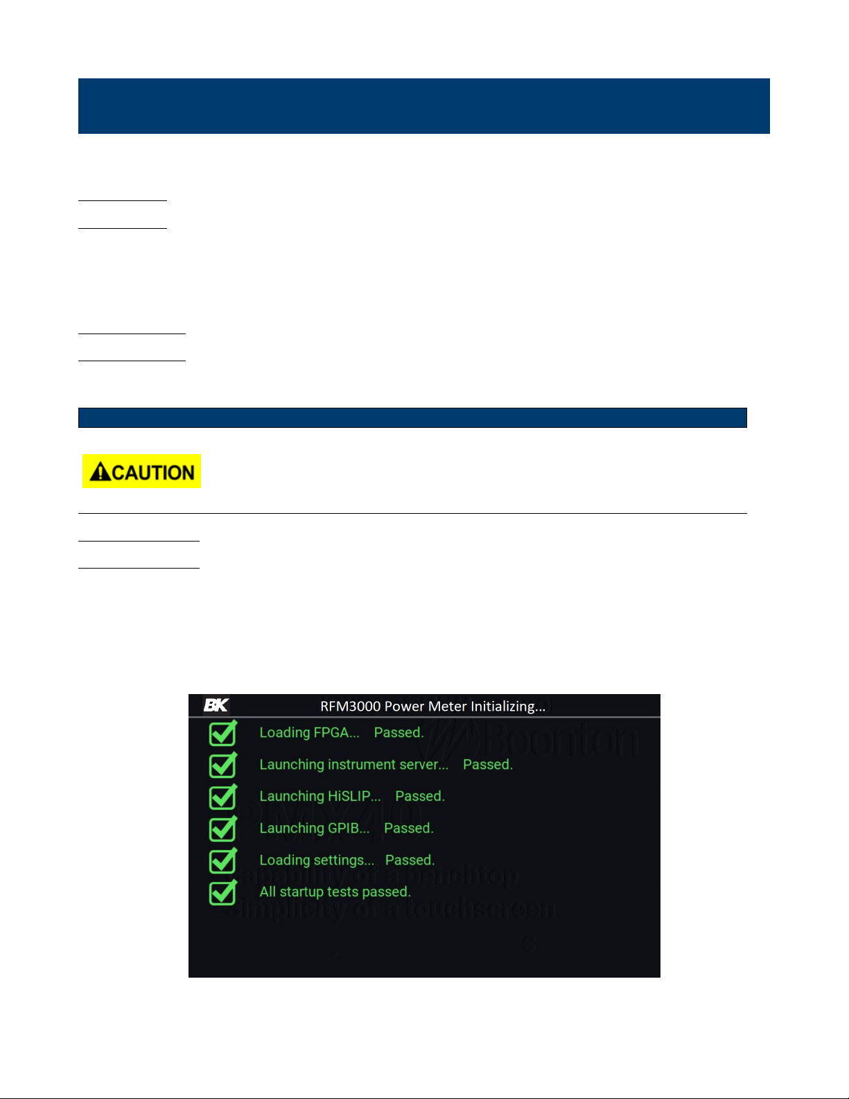
Maintenance
This section presents procedures for maintaining the RFM3000.
6.1 Safety
The RFM3000 has been designed in accordance with international safety standards, general safety precautions must be
observed during all phases of operation and maintenance. Failure to comply with the precautions listed in the Safety
Summary located in the front of this manual could result in serious injury or death. Service and adjustments should be
performed only by qualied service personnel.
6.2 Cleaning
Painted surfaces can be cleaned with a commercial spray-type window cleaner or a mild detergent and water solution.
Note:
When cleaning the instrument, do not allow cleaning uid to enter the fan intake and exhaust
vents. Avoid using chemical cleaning agents that can damage painted or plastic surfaces.
6.3 Inspection
If the RFM3000 malfunctions, perform a visual inspection of the instrument. Inspect for signs of damage caused by
excessive shock, vibration, or overheating. Inspect for broken wires, loose electrical connections, or accumulations of dust
or other foreign matter.
Correct any problems you discover, reboot the instrument, and observe the self-test results (see gure 6.1). If the
malfunction persists of the instrument fails the performance verication, contact BK Precision for service.
Figure 6.1 Self-Test Results
Page 56

Maintenance 56
6.4 Lithium Battery
The RFM3000 contains one Lithium “coin cell” battery to provide for non-volatile storage of the instrument state. This
is located on the Main Printed Circuit assembly. It should have a life of 5-10 years. When replacement is necessary, the
battery must be disposed of in strict compliance with local environmental regulations.
6.5 Software Upgrade
Instrument operating software has been loaded into the Model RFM3000 at the factory, including the BK Precision Model
RFM3000 Application Software. The Application Software will be updated from time to time to correct errors and add
new features. Users can upgrade their software by downloading it from the BK Precision webpage, bkprecision.com.
Copy the upgrade le(s) into the root directory on a USB drive, and plug the drive into one of the instrument’s USB
ports (front or rear). From the RFM3000 application, select the System menu, and select Go under Update Software.
Note:
When loading new software into the Model RFM3000, some or all stored instrument congurations and preset operating selections may be lost. Contact BK Precision for information on
which les may be aected.
Page 57

Service Information
Warranty Service: Please go to the support and service section on our website at bkprecision.com to obtain an RMA
#. Return the product in the original packaging with proof of purchase to the address below. Clearly state on the RMA
the performance problem and return any leads, probes, connectors and accessories that you are using with the device.
Non-Warranty Service: Please go to the support and service section on our website at bkprecision.com to obtain an
RMA #. Return the product in the original packaging to the address below. Clearly state on the RMA the performance
problem and return any leads, probes, connectors and accessories that you are using with the device. Customers not on
an open account must include payment in the form of a money order or credit card. For the most current repair charges
please refer to the service and support section on our website.
Return all merchandise to B&K Precision Corp. with prepaid shipping. The at-rate repair charge for Non-Warranty
Service does not include return shipping. Return shipping to locations in North America is included for Warranty Service.
For overnight shipments and non-North American shipping fees please contact B&K Precision Corp.
Include with the returned instrument your complete return shipping address, contact name, phone number and description
of problem.
B&K Precision Corp.
22820 Savi Ranch Parkway
Yorba Linda, CA 92887
bkprecision.com
714-921-9095
Page 58

LIMITED THREE-YEAR WARRANTY
B&K Precision Corp. warrants to the original purchaser that its products and the component parts thereof, will be free
from defects in workmanship and materials for a period of three years from date of purchase.
B&K Precision Corp. will, without charge, repair or replace, at its option, defective product or component parts. Returned
product must be accompanied by proof of the purchase date in the form of a sales receipt.
To help us better serve you, please complete the warranty registration for your new instrument via our website www.bkprecision.com
Exclusions: This warranty does not apply in the event of misuse or abuse of the product or as a result of
unauthorized alterations or repairs. The warranty is void if the serial number is altered, defaced or removed.
B&K Precision Corp. shall not be liable for any consequential damages, including without limitation damages resulting
from loss of use. Some states do not allow limitations of incidental or consequential damages. So the above limitation
or exclusion may not apply to you.
This warranty gives you specic rights and you may have other rights, which vary from state-to-state.
B&K Precision Corp.
22820 Savi Ranch Parkway
Yorba Linda, CA 92887
www.bkprecision.com
714-921-9095
Version: June 29, 2021
 Loading...