

Page 1

5 Commonwealth Ave
Woburn, MA 01801
Phone 781-665-1400
Toll Free 1-800-517-8431
Visit us at www.TestEquipmentDepot.com
Digital Storage Oscilloscope
User Manual
Model 2194
4
�
I ,.
.
Norm
_
gle
Sin
t
�
•
al
,
Page 2

Safety Summary
The following safety precautions apply to both operating and maintenance personnel and must be followed during all
phases of operation, service, and repair of this instrument.
Before applying power to this instrument:
• Read and understand the safety and operational information in this manual.
• Apply all the listed safety precautions.
• Verify that the voltage selector at the line power cord input is set to the correct line voltage. Operating the instrument
at an incorrect line voltage will void the warranty.
• Make all connections to the instrument before applying power.
• Do not operate the instrument in ways not specied by this manual or by B&K Precision.
Failure to comply with these precautions or with warnings elsewhere in this manual violates the safety standards of design,
manufacture, and intended use of the instrument. B&K Precision assumes no liability for a customer’s failure to comply
with these requirements.
2
Category rating
The IEC 61010 standard denes safety category ratings that specify the amount of electrical energy available and the
voltage impulses that may occur on electrical conductors associated with these category ratings. The category rating is
a Roman numeral of I, II, III, or IV. This rating is also accompanied by a maximum voltage of the circuit to be tested,
which denes the voltage impulses expected and required insulation clearances. These categories are:
Category I (CAT I): Measurement instruments whose measurement inputs are not intended to be connected to the
mains supply. The voltages in the environment are typically derived from a limited-energy transformer or a battery.
Category II (CAT II): Measurement instruments whose measurement inputs are meant to be connected to the mains
supply at a standard wall outlet or similar sources. Example measurement environments are portable
tools and household appliances.
Category III (CAT III): Measurement instruments whose measurement inputs are meant to be connected to the mains
installation of a building. Examples are measurements inside a building’s circuit breaker panel
or the wiring of permanently-installed motors.
Category IV (CAT IV): Measurement instruments whose measurement inputs are meant to be connected to the primary
power entering a building or other outdoor wiring.
Do not use this instrument in an electrical environment with a higher category rating than what is specied in this manual
for this instrument.
You must ensure that each accessory you use with this instrument has a category rating equal to or higher than the
instrument’s category rating to maintain the instrument’s category rating. Failure to do so will lower the category rating
of the measuring system.
Page 3

Electrical Power
This instrument is intended to be powered from a CATEGORY II mains power environment. The mains power should be
115 V RMS or 230 V RMS. Use only the power cord supplied with the instrument and ensure it is appropriate for your
country of use.
Ground the Instrument
To minimize shock hazard, the instrument chassis and cabinet must be connected to an electrical safety ground. This
instrument is grounded through the ground conductor of the supplied, three-conductor AC line power cable. The power
cable must be plugged into an approved three-conductor electrical outlet. The power jack and mating plug of the power
cable meet IEC safety standards.
Do not alter or defeat the ground connection. Without the safety ground connection, all accessible conductive parts
(including control knobs) may provide an electric shock. Failure to use a properly-grounded approved outlet and the
recommended three-conductor AC line power cable may result in injury or death.
3
Unless otherwise stated, a ground connection on the instrument’s front or rear panel is for a reference of potential only
and is not to be used as a safety ground. Do not operate in an explosive or ammable atmosphere.
Do not operate the instrument in the presence of ammable gases or vapors, fumes, or nely-divided particulates.
The instrument is designed to be used in oce-type indoor environments. Do not operate the instrument
• In the presence of noxious, corrosive, or ammable fumes, gases, vapors, chemicals, or nely-divided particulates.
• In relative humidity conditions outside the instrument’s specications.
• In environments where there is a danger of any liquid being spilled on the instrument or where any liquid can condense
on the instrument.
• In air temperatures exceeding the specied operating temperatures.
• In atmospheric pressures outside the specied altitude limits or where the surrounding gas is not air.
• In environments with restricted cooling air ow, even if the air temperatures are within specications.
• In direct sunlight.
This instrument is intended to be used in an indoor pollution degree 2 environment. The operating temperature range is
0∘C to 40∘C and 20% to 80% relative humidity, with no condensation allowed. Measurements made by this instrument
may be outside specications if the instrument is used in non-oce-type environments. Such environments may include
rapid temperature or humidity changes, sunlight, vibration and/or mechanical shocks, acoustic noise, electrical noise,
strong electric elds, or strong magnetic elds.
Page 4

Do not operate instrument if damaged
If the instrument is damaged, appears to be damaged, or if any liquid, chemical, or other material gets on or inside the
instrument, remove the instrument’s power cord, remove the instrument from service, label it as not to be operated,
and return the instrument to B&K Precision for repair. Notify B&K Precision of the nature of any contamination of the
instrument.
Clean the instrument only as instructed
Do not clean the instrument, its switches, or its terminals with contact cleaners, abrasives, lubricants, solvents, acids/bases,
or other such chemicals. Clean the instrument only with a clean dry lint-free cloth or as instructed in this manual. Not
for critical applications
This instrument is not authorized for use in contact with the human body or for use as a component in a life-support
device or system.
4
Do not touch live circuits
Instrument covers must not be removed by operating personnel. Component replacement and internal adjustments must
be made by qualied service-trained maintenance personnel who are aware of the hazards involved when the instrument’s
covers and shields are removed. Under certain conditions, even with the power cord removed, dangerous voltages may
exist when the covers are removed. To avoid injuries, always disconnect the power cord from the instrument, disconnect
all other connections (for example, test leads, computer interface cables, etc.), discharge all circuits, and verify there
are no hazardous voltages present on any conductors by measurements with a properly-operating voltage-sensing device
before touching any internal parts. Verify the voltage-sensing device is working properly before and after making the
measurements by testing with known-operating voltage sources and test for both DC and AC voltages. Do not attempt
any service or adjustment unless another person capable of rendering rst aid and resuscitation is present.
Do not insert any object into an instrument’s ventilation openings or other openings.
Hazardous voltages may be present in unexpected locations in circuitry being tested when a fault condition in the circuit
exists.
Fuse replacement must be done by qualied service-trained maintenance personnel who are aware of the instrument’s fuse
requirements and safe replacement procedures. Disconnect the instrument from the power line before replacing fuses.
Replace fuses only with new fuses of the fuse types, voltage ratings, and current ratings specied in this manual or on
the back of the instrument. Failure to do so may damage the instrument, lead to a safety hazard, or cause a re. Failure
to use the specied fuses will void the warranty.
Page 5

Servicing
Do not substitute parts that are not approved by B&K Precision or modify this instrument. Return the instrument to
B&K Precision for service and repair to ensure that safety and performance features are maintained.
For continued safe use of the instrument
• Do not place heavy objects on the instrument.
• Do not obstruct cooling air ow to the instrument.
• Do not place a hot soldering iron on the instrument.
• Do not pull the instrument with the power cord, connected probe, or connected test lead.
• Do not move the instrument when a probe is connected to a circuit being tested.
Working Environment
5
Environment
This instrument is intended for indoor use and should be operated in a clean, dry environment.
Temperature
Operating: 0℃ to +40℃
Non-operation:-20℃ to +60℃
Note:
Direct sunlight, radiators, and other heat sources should be taken into account when assessing the ambient temperature.
Humidity
Operating: 85% RH, 40 ℃, 24 hours
Non-operating: 85% RH, 65 ℃, 24 hours
Altitude
Operating: less than 3 Km
Non-operation: less than 15 Km
Installation (overvoltage) Category
This product is powered by mains conforming to installation (overvoltage) category II.
Degree of Pollution
The oscilloscopes may be operated in environments of Pollution Degree II.
Note:
Degree of Pollution II refers to a working environment which is dry and non-conductive pollution occurs. Occasional
temporary conductivity caused by condensation is expected.
IP Rating
IP20 (as dened in IEC 60529).
Page 6
Compliance Statements
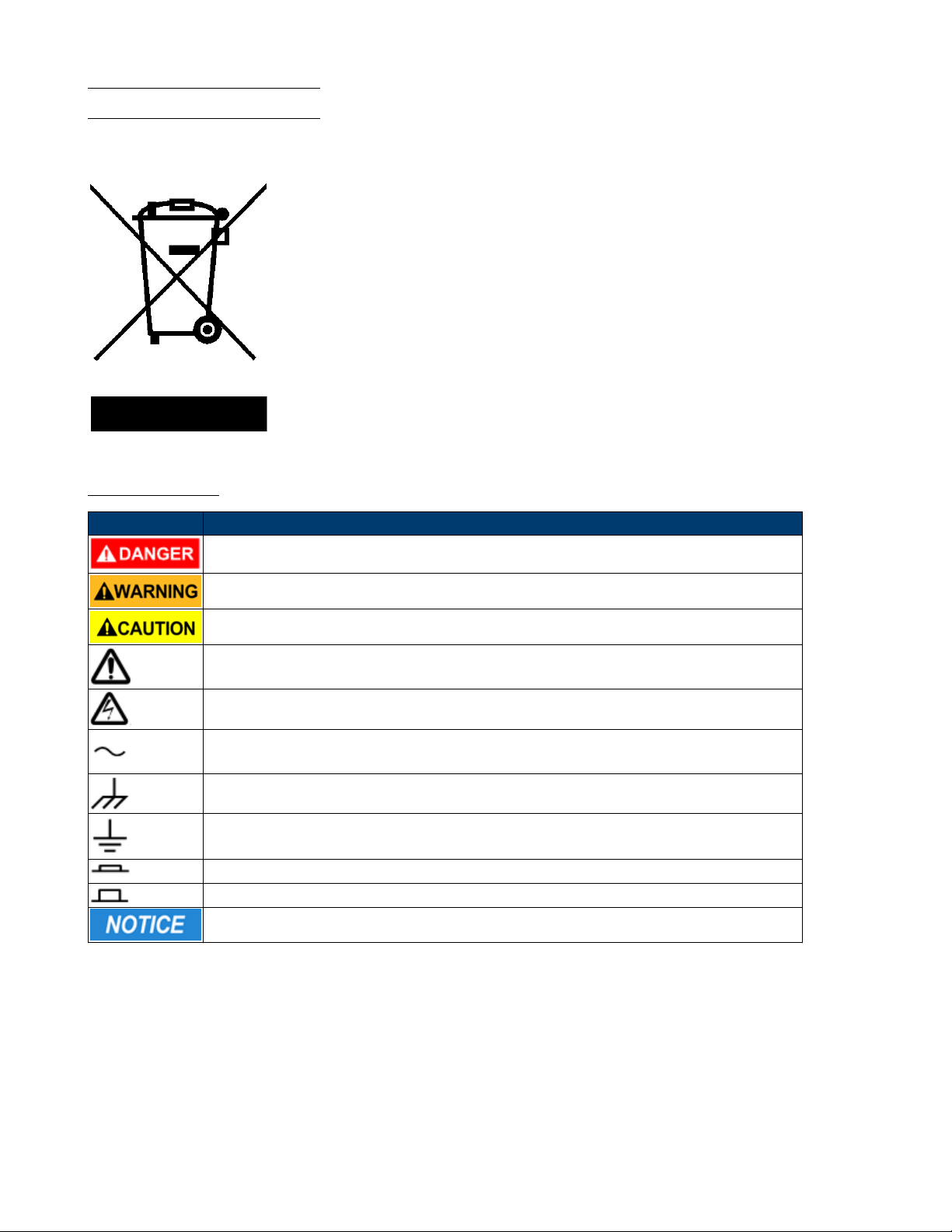
Disposal of Old Electrical & Electronic Equipment (Applicable in the European Union and other European
countries with separate collection systems)
This product is subject to Directive 2002/96/EC of the European Parliament
and the Council of the European Union on waste electrical and electronic equipment
(WEEE), and in jurisdictions adopting that Directive, is marked as being put on the
market after August 13, 2005, and should not be disposed of as unsorted municipal
waste. Please utilize your local WEEE collection facilities in the disposition of this
product and otherwise observe all applicable requirements.
Safety Symbols
6
Symbol Description
indicates a hazardous situation which, if not avoided, will result in death or serious injury.
indicates a hazardous situation which, if not avoided, could result in death or serious injury
indicates a hazardous situation which, if not avoided, will result in minor or moderate injury
Refer to the text near the symbol.
Electric Shock hazard
Alternating current (AC)
Chassis ground
Earth ground
This is the In position of the power switch when instrument is ON.
This is the Out position of the power switch when instrument is OFF.
is used to address practices not related to physical injury.
Page 7

Contents
1 General Information 11
1.1 Product Overview 11
1.2 Features 11
1.3 Contents 11
1.4 Dimensions 12
1.5 Front Panel Overview 13
1.6 Rear Panel Overview 14
1.7 Display Overview 15
2 Getting Started 16
2.1 Input Power Requirements 16
2.2 Fuse Requirements and Replacement 16
2.3 Preliminary Check 17
2.3.1 Verify AC Input Voltage 17
2.3.2 Connect Power 17
2.3.3 Self-Test 18
2.3.4 Self-Cal 18
2.3.5 Check Model and Firmware Version 18
2.3.6 Function Check 19
2.4 Probe Safety 20
3 Vertical Controls 22
3.1 Enable Channel 22
3.2 Channe Menu 22
3.2.1 Channel Coupling 23
3.2.2 Bandwidth Limit 23
3.2.3 Adjust 23
3.2.4 Probe 24
3.2.5 Unit 24
3.2.6 Deskew 25
3.2.7 Invert 25
3.2.8 Oset 25
3.2.9 Trace Visible/Hidden 26
4 Horizontal Control 27
4.1 Horizontal Scale 27
4.2 Zoom 27
4.3 Roll Mode 28
4.4 Trigger Delay 28
5 Sample Control 29
5.1 Run Control 29
5.2 Sampling Theory 29
5.3 Sample Rate 29
5.4 Bandwidth and Sample Rate 30
5.5 Memory Depth 31
5.6 Sampling Mode 32
5.7 Interpolation Method 32
5.8 Acquisition Mode 33
5.9 Average 35
5.10 Eres Acquisition 35
5.11 Horizontal Format 35
5.12 Sequence Mode 37
Page 8

6 Trigger 38
6.1 Trigger Source 38
6.2 Trigger Mode 39
6.3 Trigger Level 40
6.4 Trigger Coupling 41
6.5 Trigger Holdo 42
6.6 Noise Rejection 43
6.7 Trigger Types 43
6.7.1 Edge Trigger 44
6.7.2 Slope Trigger 45
6.7.3
46
6.7.4 Video Trigger 48
6.7.5 Window Trigger 51
6.7.6 Interval Trigger 54
6.7.7 Dropout Trigger 56
6.7.8 Runt Trigger 58
6.7.9 Pattern Trigger 60
7 Serial Trigger and Decode 62
7.1 I2C Trigger and Serial Decode 62
7.1.1 Setup for I2C Signals 62
7.1.2 I2C Trigger 63
7.1.3 I2C Serial Decode 66
7.2 SPI Trigger and Serial Decode 67
7.2.1 Setup for SPI Signals 67
7.2.2 SPI Trigger 71
7.2.3 SPI Serial Decode 72
7.3 UART Trigger and Serial Decode 73
7.3.1 Setup for UART Signals 73
7.3.2 UART Trigger 74
7.3.3 UART Serial Decode 75
7.4 CAN Trigger and Serial Decode 77
7.4.1 Setup for CAN Signals 77
7.4.2 CAN Trigger 77
7.4.1 CAN Serial Decode 79
7.5 LIN Trigger and Serial Decode 80
7.5.1 Setup for LIN Signals 80
7.5.2 LIN Trigger 81
7.5.1 Interpreting LIN Decode 83
8
8 Reference Waveform 84
8.1 Save REF Waveform to Internal Memory 84
8.2 Display REF Waveform 84
8.3 Adjust REF Waveform 85
8.4 Clear Ref Waveform 85
9 Math 86
9.1 Units for Math Waveforms 86
9.2 Math Operators 87
9.2.1 Addition or Subtraction 87
9.2.2 Multiplication and Division 88
9.2.3 FFT Operation 89
9.3 Math Function Operation 93
9.3.1 Dierentiate 93
9.3.2 Integrate 94
9.3.3 Square Root 94
Page 9

10 Cursors 96
10.1 X Cursors 96
10.2 Y Cursors 97
10.3 Make Cursor Measurements 98
11 Measure 99
11.1 Type of Measurement 99
11.1.1 Voltage Measurements 99
11.1.2 Time Measurements 101
11.1.3 Delay Measurements 101
11.2 Automatic Measurement 102
11.3 All Measurement 104
11.4 Gate Measurement 105
11.5 Clear Measurement 105
12 Display 106
12.1 Display Type 106
12.2 Color Display 107
12.3 Persistence 108
12.4 Clear Display 109
12.5 Grid Type 109
12.6 Intensity 109
12.7 Grid Brightness 109
12.8 Transparence 110
9
13 Save and Recall 111
13.1 Save Type 111
13.2 Internal Save and Recall 112
13.3 External Save and Recall 113
13.4 Disk Management 115
13.4.1 Create a New File or Folder 115
13.4.2 Delete a File or Folder 116
13.4.3 Rename a File or Folder 116
14 System Settings 117
14.1 View System Status 117
14.2 Self Cal 118
14.3 Quick-Cal 118
14.4 Sound 119
14.5 Language 119
14.6 Pass/Fail Test 119
14.6.1 Set and Perform a Pass/Fail Test 120
14.6.2 Save and Recall Test Mask 121
14.7 IO Set 123
14.7.1 LAN 123
14.7.2 USB Device 124
14.8 Update Firmware and Conguration 124
14.9 Do Self-Test 125
14.9.1 Screen Test 125
14.9.2 Keyboard Test 126
14.9.3 LED Test 127
14.10 Screen Saver 128
14.11 Reference Position 129
14.12 Power On Line 129
15 Search 130
15.1 Setting 130
15.2 Results 131
Page 10

10
16 Navigate 133
16.1 Time Navigate 133
16.2 History Frame Navigate 133
16.3 Search Event Navigate 133
17 History 134
18 Factory Setup 135
19 Troubleshooting 136
20 Service Information 138
21 LIMITED THREE-YEAR WARRANTY 139
Page 11

General Information
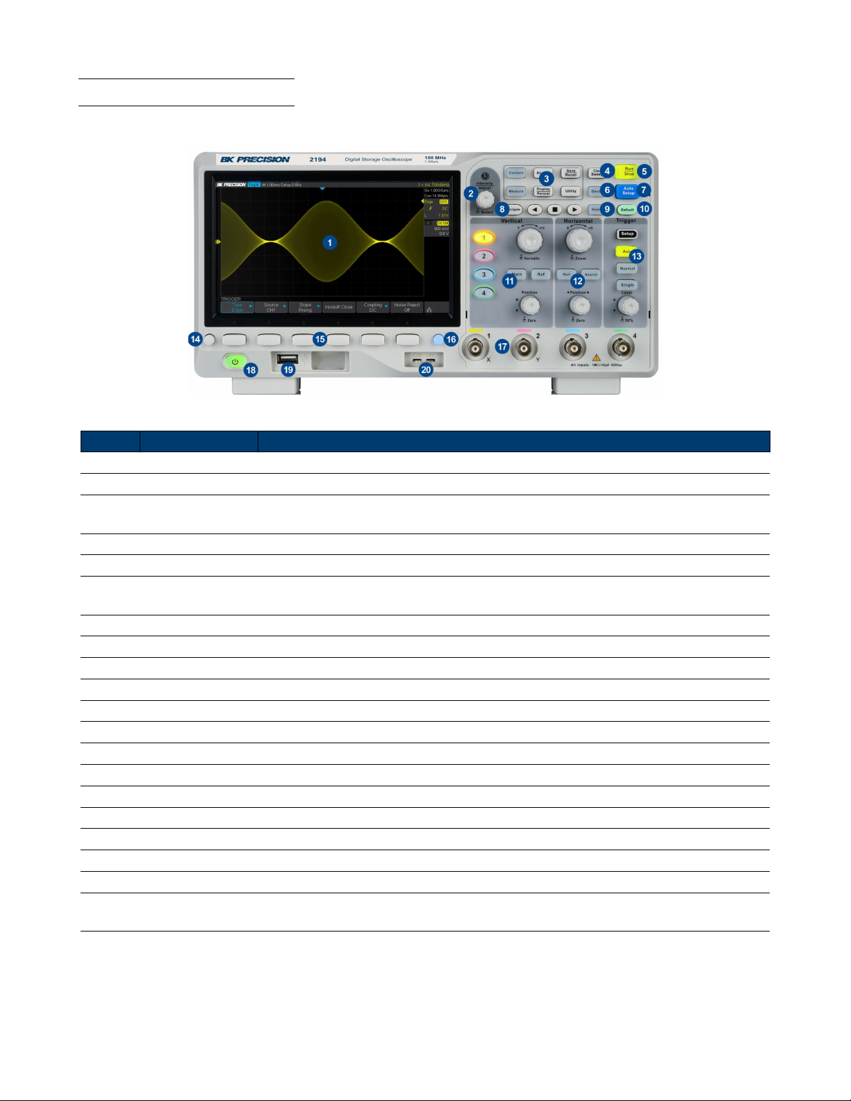
1.1 Product Overview
Figure 1.1 2194 Front View
The B&K Precision 2194 digital storage oscilloscope (DSO) is a portable benchtop instrument used for making measurements of signals and waveforms.
This oscilloscope provides 100 MHz of bandwidth in a 4-channel conguration with a maximum sample rate of 1 GSa/s
and best-in class memory depth of 14 Mpts.
1.2 Features
– 4 channels with 100 MHz bandwidth
– Single channel real-time sampling rate of up to 1 GSa/s
– 14 Mpts memory depth
– Standard USB host, USBTMC device, and LAN ports
1.3 Contents
Inspect the instrument mechanically and electrically upon receiving it. Unpack all items from the shipping carton, and
check for any obvious signs of physical damage that may have occurred during transportation. Report any damage to
the shipping agent immediately. Save the original packing carton for possible future reshipment. Every oscilloscope is
shipped with the following contents:
– 1 x 2194 Digital Storage Oscilloscope
– AC Power Cord
– USB type A to type B cable.
– 4 x 1:1/10:1 Passive Oscilloscope Probes
– Certicate of Calibration
– Test Report
Page 12

General Information 12
Note:
Ensure the presence of all the items above. Contact the distributor if anything is missing.
1.4 Dimensions
The 2194 digital storage oscilloscope’s dimensions are approximately: 312.00 mm (12.28 in) x 151.00 mm (5.94 in) x
132.60 mm (5.22 in) (W x H x D).
Figure 1.2 Front View Dimensions
Figure 1.3 Top View Dimensions
Page 13
General Information 13
1.5 Front Panel Overview
The front panel interface allows for control of the unit.
Figure 1.4 Front Panel
Item Name Description
1 LCD Display Visual presentation of the device function and measurements.
2 Intensity Adjust Universal knob.
3
4 Numeric Keypad Used to enter precise values
5 Rotary Knob Used to navigate menus or congure parameters
6 Navigation Keys
7 CH 2 Terminals Serves as output or input terminals of CH 2 depending on the set functionality
8 Function Keys Frequently used function such as Home, Trig, Menu, ESC, and On/O keys
9 CH 1 Terminals Serves as output or input of CH 1 depending on the set functionality
10 Softkeys Used to invoke any functions displayed above them.
11 Power Switch Power the unit ON or OFF
12 Horizontal Control
13 Auto Set the trigger mode to auto.
14 Menu On/O Enable/disable the menu bar.
15 Softkeys Used to invoke any functions displayed above them.
16 Print Shortcut key for the save function.
17 Input Channels Input channels (1 MΩ BNC)
18 Power Button Power the unit ON or OFF.
19 USB Host Port USB port used to connect ash drives. (Type A)
20
Common
Function Keys
Probe
Compensation
Used to invoke the functions displayed above them.
Used to navigate menus. The enter key can be used to select a menu or enter a parameter
Probe compensation/ground terminal.
Table 1.1 Front Panel
Page 14

General Information 14
1.6 Rear Panel Overview
Figure 1.5 Rear Panel Overview
Item Name Description
1 Handle Handle for easy carrying of the instrument.
2 Safety Lock Hole
3 LAN Connect an ethernet cable to remotely control the unit over the network.
4 USB Interface Connect a USB type B to type A to remotely control the unit.
5
6
Pass/Fail or
Trigger Out
AC Power Input
& Fuse Box
Locks the instrument to a xed location using the security lock via the lock hole.
The lock is not included.
Output a signal that reects the current waveform capture rate of the oscilloscope at
each trigger or a pass/fail test pulse.
Houses the fuse as well as the AC input .
Table 1.2 Rear Panel
Page 15

General Information 15
1.7 Display Overview
Figure 1.6 Display Overview
Item Name Description
1 Trigger Status Displays the trigger status.
2
3
4 Menu Bar Displays the available options in the selected menu.
USB Host
Port Indicator
LAN Port
Indicator
Indicates that a USB is connected to the instrument.
Indicates the status of the LAN connection.
Table 1.3 Display Overview
Page 16

Getting Started
Before connecting and powering up the instrument, review the instructions in this chapter.
2.1 Input Power Requirements
The oscilloscope has a universal AC input that accepts line voltage and frequency input within:
100 - 240 V (+/- 10%), 50/60 Hz (+/- 5%)
100 - 127 B, 400 Hz
50 W Max
Before connecting to an AC outlet or external power source, be sure that the power switch is in the OFF position and
verify that the AC power cord, including the extension line, is compatible with the rated voltage/current and that there
is sucient circuit capacity for the power supply. Once veried, connect the cable rmly.
The included AC power cord is safety certied for this instrument operating in rated range. To change a cable or add
an extension cable, be sure that it can meet the required power ratings for this instrument. Any misuse with wrong or
unsafe cables will void the warranty.
SHOCK HAZARD:
The power cord provides a chassis ground through a third conductor. Verify that your power outlet is of the
three conductor type with the correct pin connected to earth ground.
2.2 Fuse Requirements and Replacement
For continued re protection at all line voltages replace only with a 1.25 A / 250 V "F" rated, 5 x 20 mm
fuse.
For safety, no power should be applied to the instrument while changing line voltage operation. Disconnect all
cables connected to the instrument before proceeding.
Page 17

Getting Started 17
Check and/or Change Fuse
– Locate the fuse box next to the AC input connector in the rear panel. (See gure 1.5)
– Insert a small athead screwdriver into the fuse box slit to pull and slide out the fuse box as indicated below.
– Check and replace fuse if necessary. (See gure 2.1)
Figure 2.1 Fuse Removal
Any disassembling of the case or changing the fuse not performed by an authorized service technician will void
the warranty of the instrument
2.3 Preliminary Check
Complete the following steps to verify that the oscilloscope is ready for use.
2.3.1 Verify AC Input Voltage
Verify proper AC voltages are available to power the instrument.
The AC voltage range must meet the acceptable specication stated in section Input Power Requirements.
2.3.2 Connect Power
Connect the AC power cord to the AC receptacle in the rear panel and press the power switch to turn on the instrument.
The instrument will have a boot up screen while loading, after which the main screen will be displayed.
Page 18
Getting Started 18
2.3.3 Self-Test
The instrument has 3 self-test option to test the screen ,keyboard, and the LED back light.
To perform the self-test, please refer to the Self Test section for further instructions.
2.3.4 Self-Cal
Self option runs an internal self-calibration procedure that will check and adjust the instrument. To perform the selfcalibration refer to the Self-Calibration section for further instructions.
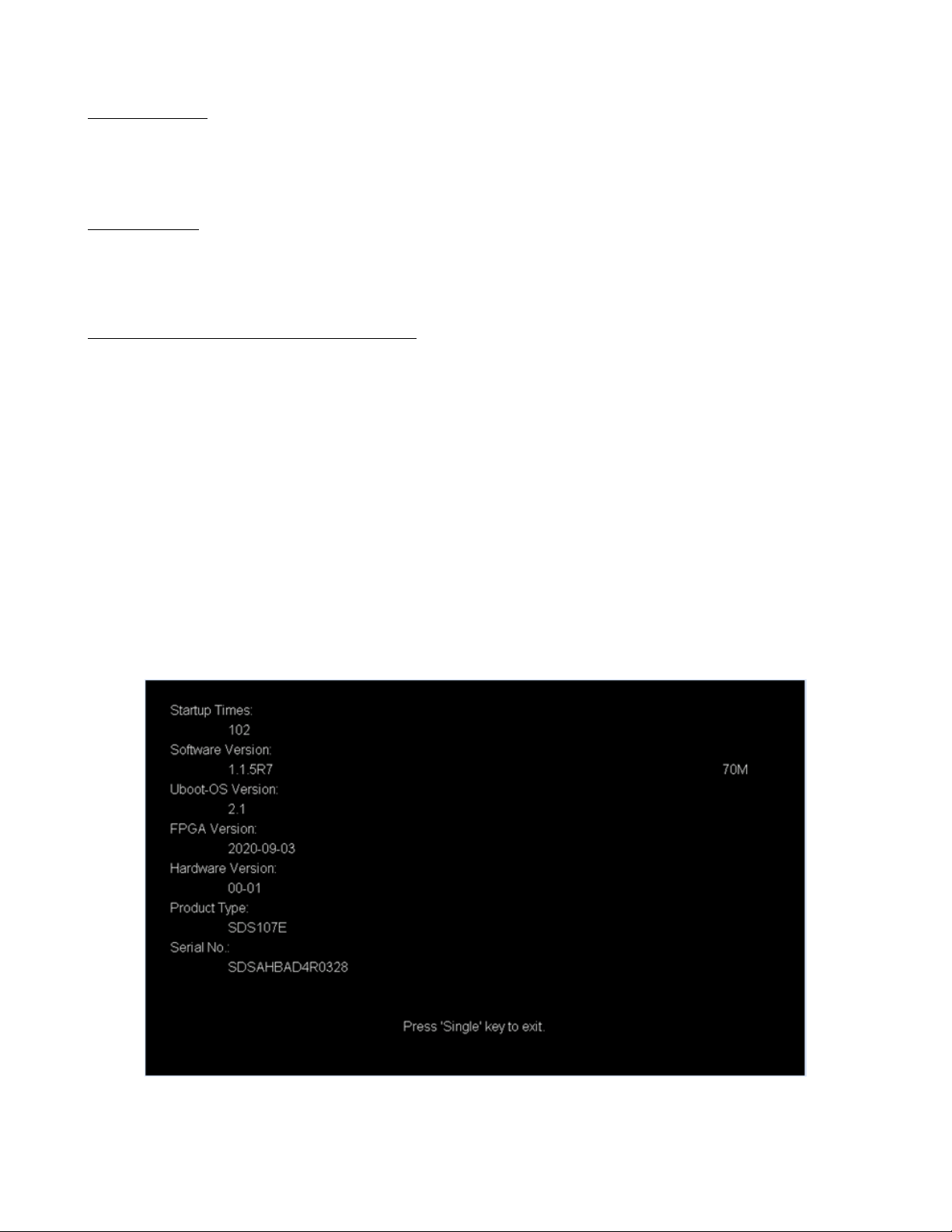
2.3.5 Check Model and Firmware Version
The model and rmware version can be veried from within the menu system.
To view the model and rmware version:
Press the Utility button and use the softkeys to select the System Status option. The following information will be
displayed:
– Startup Times
– Software Version
– Uboot-Os Version
– FPGA Version
– Hardware Version
– Product Type
– Serial NO
Press the Single key to exit.
Figure 2.2 System Status
Page 19

Getting Started 19
2.3.6 Function Check
Follow the steps below to do a quick check of the oscilloscope’s functionality.
1. Power on the oscilloscope. Press Default Setup to show the result of the self-check.
– The probe default attenuation is 1X.
2. Set the switch to 1X on the probe and connect the probe to channel 1.
– To do this align the slot in the probe connector with the key on the CH1 BNC, push to connect, and twist to the
right to lock the probe in place.
– Connect the probe tip and reference lead to the Probe Comp connectors.
3. Press the AUTO button to show the square wave with 1 kHz frequency and 3V peak to peak .
Figure 2.3 3 Vpp Square Wave
4. Repeat steps 1 to 3 for the remaining channels.
Page 20
Getting Started 20
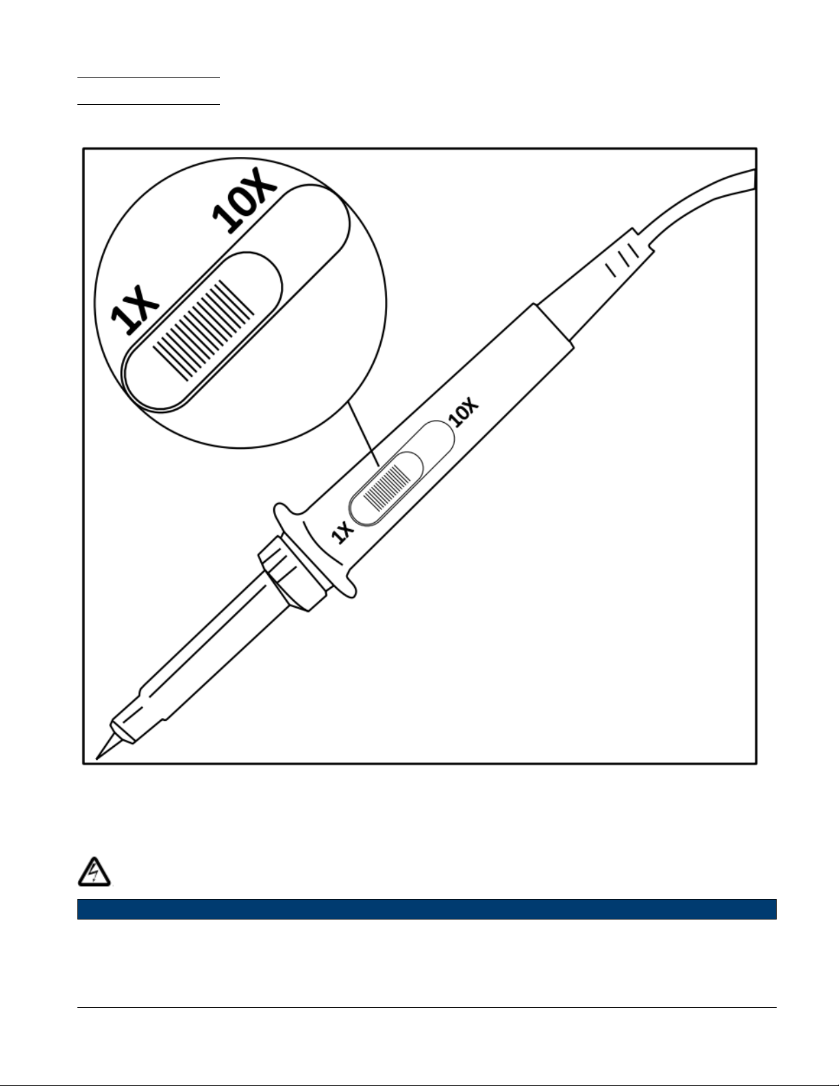
2.4 Probe Safety
A guard around the probe body provides a nger barrier for protection from electric shock.
Figure 2.4 Probe
Connect the probe to the oscilloscope and connect the ground terminal to the ground before you take any measurements.
Shock Hazard:
To avoid electric shock when using the probe, keep ngers behind the guard on the probe body. To avoid electric shock
while using the probe, do not touch metallic portions of the probe head while it is connected to a voltage source.
Connect the probe to the oscilloscope and connect the ground terminal to ground before you take any measurements.
Page 21

Getting Started 21
Probe Attenuation
Probes are available with various attenuation factors which aect the vertical scale of the signal. The Probe Check
function veries that the probe attenuation option matches the attenuation of the probe.
Press CH 1 once to open the channel menu. Use the softkeys to navigate to page 1/2 and select the Probe option.
Select the probe option that matches the attenuation of the probe.
Note:
The default setting for the Probe option is 1 X.
Verify that the attenuation switch on the probe matches the Probe option in the oscilloscope. Switch settings are 1 X
and 10 X.
Probe Compensation
Before taking any measurements using a probe, verify the compensation of the probe and adjust it to match the channel
inputs.
To match your probe to the input channel:
1. Set the channel’s probe attenuation to 10X.
– Press the CH # key corresponding to the channel the probe is connected to.
– Use the softkeys to navigate to page 1.
– Use the softkeys to select Probe.
– Use the Intensity Adjust knob to select 10X.
2. Attach the probe tip to the Compensation Signal Output Terminal 3 V(Cal) connector and the reference lead to
the Probe Ground terminal connector.
– Press the Auto Setup key to display the square wave.
3. Check the shape of the displayed waveform.
Undercompensated Correctly Compensated Overcompensated
Figure 2.5 Probe Compensation
4. If necessary, adjust your probe’s compensation trimmer pot.
Page 22
Vertical Controls
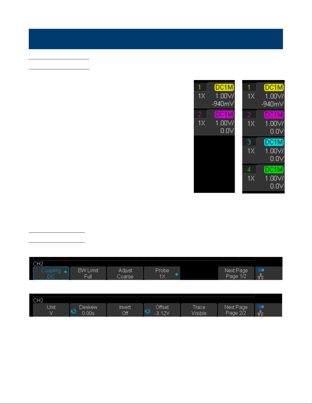
3.1 Enable Channel
The 2194 provides 4 analog input channels. To enable a channel press
the corresponding channel button located on the vertical controls.
The enabled channels can be veried on the right side of the display
screen.
To disable a channel:
Press the correponding channel key. Once the key has been highlighted
by the LED press the channel key again.
– Pressing the channel key of the currently selected channel once will
disable the channel.
and 2 Enabled
3.2 Channe Menu
Figure 3.2 shows the channel 2 menu that is displayed after pressing the CH 2 key.
Channel Menu Page 1/2
Channel Menu Page 2/2
Figure 3.2 CH 2 Menu
Channels 1
Figure 3.1 Enabled Channels
All Channels
Enabled
Page 23

Vertical Controls 23
3.2.1 Channel Coupling
Coupling mode lters out the undesired signals.
Press the corresponding CH button, then use the softkeys to select Coupling.
Turn the Universal Knob to select the desired coupling method.
Note:
The current coupling method is displayed in the channel label at the right side of the screen. Pressing the Coupling
softkey continuously switches between the available coupling method.
• DC Coupling: The DC and AC components of the signal under test are both passed.
• AC Coupling: The DC components of the signal under test are blocked.
• GND Coupling: The DC and AC components of the signal under test are both blocked.
3.2.2 Bandwidth Limit
Sets the bandwidth limit to reduce display noise.
Press the CH button of the channel to be congured.
Use the softkeys to select BW Limit. (The bandwidth limit will alternate between Full and 20 M)
• Full: The high frequency components of the signal under test can pass the channel.
• 20 M: The high frequency components exceeding 20 MHz are attenuated.
3.2.3 Adjust
Adjust the vertical scale sensitivity of the selected channel.
The vertical scale is adjusted using the Vertical Variable Knob.
Press the CH button of the channel to be congured.
Use the softkeys to select Adjust. (The scale will alternate between Fine and Coarse)
If the amplitude of the input waveform is a little bit greater than the full scale under the current scale and the amplitude
would be a little bit lower if the next scale is used, ne adjustment can be used to improve the amplitude of waveform
display to view signal details.
• Fine adjustment: Adjust the vertical scale within a relatively smaller range to improve vertical resolution.
– For example: 2 V/div, 1.98V/div, 1.96V/div, 1.94 V/div, ...1 V/div.
• Coarse: Adjust the vertical scale in a 1-2-5 step.
– For example: 1 mV/div, 2 mV/div, 5 mV/div, 10 mV/div 200 mV/div, 500 mV/div,... 10 V/div.
The scale information in the channel label at the right side of the screen will change accordingly during the adjustment.
The adjustable range of the vertical scale is related to the probe ratio currently set.
Page 24

Vertical Controls 24
Note:
Push the Vertical Variable Knob to quickly switch between Coarse and Fine adjustment.
3.2.4 Probe
Sets the probe attenuation factor to match the type of probe being used.
1. Press the CH button of the channel to be congured.
2. Use the softkeys to select Probe.
3. Use the softkeys to select Probe once more.
4. Use the Universal Knob to select the probe attenuation.
Table 3.1 shows the probe attenuation factors.
Setting Description
0.1X .01 : 1
0.2X .02 : 1
0.5X .05 : 1
1X 1 : 1
2X 2 : 1
5X 5 : 1
10X 10 : 1
... ...
10000X 10000 : 1
Table 3.1 Attenuation Factor
To customize the probe attenuation factor:
Press the Probe softkey, select Custom, and then press the Custom softkey.
Use the Universal Knob to set the desired probe attenuation ratio.
The range is [1E-6,1E6].
3.2.5 Unit
Selects the amplitude display unit for the selected channel.
The available units are V and A.
1. Press the CH button of the channel to be congured.
2. Use the softkeys to navigate to page 2/2.
3. Use the softkeys to select Unit and alternate between V and A.
The default unit is V.
Page 25
Vertical Controls 25
3.2.6 Deskew
Adjust the dierence of phase between the channel.
The Valid range of each channel is±100 ns.
1. Press the CH button of the channel to be congured.
2. Use the softkeys to navigate to page 2/2.
3. Use the softkeys to select Deskew.
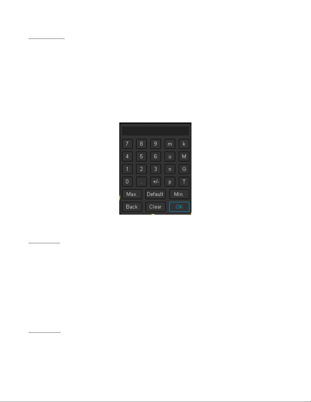
4. Turn the Universal Knob to change deskew.
– Pushing the Universal Knob open the keypad.
Figure 3.3 Deskew Keypad
3.2.7 Invert
Invert the voltage values of the displayed waveform.
Inverting a channel aects how the channel is displayed, all the results of any math function selected, and measurement
functions.
To invert the waveform:
– Press the CH button of the channel to be congured.
– Use the softkeys to navigate to page 2/2.
– Use the softkeys to toggle Invert On and O.
3.2.8 Oset
Oset the vertical position of the displayed waveform.
The Valid range of each channel is±100 V.
1. Press the CH button of the channel to be congured.
2. Use the softkeys to navigate to page 2/2.
Page 26

Vertical Controls 26
3. Use the softkeys to select Oset.
4. Turn the Universal Knob to change deskew.
– Pushing the Universal Knob open the keypad.
Figure 3.4 Oset Keypad
Note:
The Vertical Position Knob can be used to oset the waveform’s vertical position without having to enter the channel’s menu. Pushing the Vertical Position Knob will zero vertical position.
3.2.9 Trace Visible/Hidden
Sets whether waveform of the selected channel is visible or hidden.
To toggle between visible and hidden:
1. Press the CH button of the channel to be congured.
2. Use the softkeys to navigate to page 2/2.
3. Use the softkeys to select Trace.
Page 27

Horizontal Control
4.1 Horizontal Scale
Turn the Horizontal Scale Knob to adjust the horizontal time base. Turning the knob clockwise reduces the horizontal
time base. Turning the knob counterclockwise increases the time base.
The time base information at the upper left corner of the screen will change accordingly during the adjustment. The
2194 horizontal scale has a range from 2ns/div to 100s/div.
The Horizontal Scale Knob works (in the Normal time mode) while acquisitions are running or when they are stopped.
When in run mode, adjusting the horizontal scale knob changes the sample rate.
When stopped, adjusting the horizontal scale knob lets you zoom into acquired data.
4.2 Zoom
Zoom is a horizontally expanded version of the normal display. You can use Zoom to locate and horizontally expand part
of the normal window for a more detailed (higher- resolution) analysis of signals.
Press the Horizontal Scale Knob to enable the zoom function, and press the button again to turn disable the function.
When Zoom enabled, the display divides in half. The top half of the display shows the normal time base window and
the bottom half displays a faster Zoom time base window.
Figure 4.1 Zoom Mode
The area of the normal display that is expanded is outlined with a box and the rest of the normal display is ghosted. The
box shows the portion of the normal sweep that is expanded in the lower half.
Page 28

Horizontal Control 28
To change the time base for the zoom window, turn the Horizontal Scale Knob. The Horizontal Position Knob sets
the left- to- right position of the zoom window.
The delay value, which is the time displayed relative to the trigger point is momentarily displayed in the upper right
corner of the display when the Horizontal Position Knob is turned. Negative delay values indicate you’re looking at a
portion of the waveform before the trigger event, and positive values indicate you’re looking at the waveform after the
trigger event.
To change the time base of the normal window, disable Zoom, then turn the Horizontal Scale Knob.
4.3 Roll Mode
In Roll mode the waveform moves slowly across the screen from right to left. It operates on time base settings of 50
ms/div and slower. If the current time base setting is faster than the 50 ms/div limit, it will be set to 50 ms/div when
Roll mode is entered.
In Roll mode there is no trigger. The xed reference point on the screen is the right edge of the screen and refers to
the current moment in time. Events that have occurred are scrolled to the left of the reference point. Since there is no
trigger, no pre- trigger information is available.
To enter Roll mode press the Roll button.
To stop the display, press the Run/Stop button.
To clear the display and restart an acquisition in Roll mode, press the Run/Stop button again.
To exit Roll mode press the Roll button.
Note:
Use Roll mode on low- frequency waveforms to yield a display much like a strip chart recorder.
4.4 Trigger Delay
Turn the Horizontal Position Knob on the front panel to adjust the trigger delay of the waveform. During the
modication, waveforms of all the channels would move left or right and the trigger delay message at the upper-right
corner of the screen would change accordingly. Press down this knob to quickly reset the trigger delay.
Changing the delay time moves the trigger point (solid inverted triangle) horizontally and indicates how far it is from the
time reference point. These reference points are indicated along the top of the display grid.
All events displayed left of the trigger point happened before the trigger occurred. These events are called pre- trigger
information, and they show events that led up to the trigger point.
Everything to the right of the trigger point is called post- trigger information. The amount of delay range (pre- trigger
and post- trigger information) available depends on the time/div selected and memory depth.
The position knob works (in Normal time mode) while acquisitions are running or when they are stopped.
Page 29

Sample Control
5.1 Run Control
Press the Run/Stop or the Single key to stop the sampling system of the scope.
• Running: When the Run/Stop key is green, the oscilloscope is continuously acquiring data.
– To stop acquiring data, press the Run/Stop key.
– When the Run/Stop button is red, data acquisition is stopped.
– Red "Stop" text is displayed next to the trademark logo in the status line at the top of the display.
– To start acquiring data, press Run/Stop.
• Single: Clears the display, the trigger mode is temporarily set to Normal (to keep the oscilloscope from auto- triggering
immediately), the trigger circuitry is armed, the Single key is illuminated, and the oscilloscope waits until a user dened
trigger condition occurs before it displays a waveform.
– When the oscilloscope triggers, the single acquisition is displayed and the oscilloscope is stopped (the Run/Stop
button is illuminated in red).
– Press the Single key again to clear the current waveform and acquire a new one.
Note:
The Single run control lets you view a single shot events without subsequent waveform data overwriting the display. Use
Single when you want maximum memory depth for pan and zoom.
5.2 Sampling Theory
The Nyquist sampling theorem states that for a limited bandwidth (band- limited) signal with maximum frequency 𝑓
the equally spaced sampling frequency 𝑓𝑆must be greater than twice the maximum frequency 𝑓
the signal be uniquely reconstructed without aliasing.
𝑓
𝑀𝐴𝑋
= 𝐹
= 𝑁𝑦𝑞𝑢𝑖𝑠𝑡 𝑓𝑟𝑒𝑞𝑢𝑒𝑛𝑐𝑦(𝑓𝑁) = 𝑓𝑜𝑙𝑑𝑖𝑛𝑔 𝑓𝑟𝑒𝑞𝑢𝑒𝑛𝑐𝑦
𝑆/2
, in order to have
𝑀𝐴𝑋
𝑀𝐴𝑋
5.3 Sample Rate
The maximum sample rate of the oscilloscope is 1G Sa/s. The actual sample rate of the oscilloscope is determined by
the horizontal scale. See section Horizontal Scale
The actual sample rate is displayed in the information area at the upper- right corner of the screen.
,
Figure 5.1 Actual Sample Rate
Page 30

Sample Control 30
The sample rate aect the waveform in the following manner :
• Waveform Aliasing: Aliasing occurs when the signal is under-sampled. The signal is distorted by low frequencies
falsely being reconstructed from an insucient number of sample points.
Figure 5.2 Low Sample Rate
5.4 Bandwidth and Sample Rate
An oscilloscope’s bandwidth is typically described as the lowest frequency at which input signal sine waves are attenuated
by 3 dB (-30% amplitude error).
The sampling theory requires the sample rate to be 𝑓𝑆= 2 ∗ 𝑓𝐵𝑊. However, the theory assumes there are no frequency
components above 𝑓
𝑀𝐴𝑋(𝑓𝐵𝑊
in this case) and it requires a system with an ideal brick-wall frequency response.
Figure 5.3 Brick-Wall Frequency Response
Digital signals have frequency components about the fundamental frequency (Square waves are made up of sine waves at
the fundamental frequency and an innite number of odd harmonics), and typically, for 500 MHz bandwidths and below,
oscilloscopes have a Gaussian frequency response.
Page 31

Sample Control 31
Figure 5.4 Bandwidth Limiting
In practice, an oscilloscope’s sample rate should be four or more times its bandwidth: 𝑓𝑠= 4𝑥𝑓𝐵𝑊. Doing so causes less
aliasing, and aliased frequency components have a great amount of attenuation.
5.5 Memory Depth
Memory Depth refers to the number of waveform points that the oscilloscope can store in a single trigger sample. It
reects the storage ability of the sample memory.
To set the Memory Depth:
1. Press the Acquire key.
2. Use the softkeys to select Mem Depth (Page 1/2).
3. Turn the Universal Knob to navigate the available option.
4. Push the Universal Knob to set the selected option.
The actual memory depth is displayed in the information area at the upper right corner of the screen.
Single Channel
Mode
14 k 7 k 3.5 k
140 k 70 k 35 k
1.4 M 700 k 350 k
14 M 7 M 3.5 M
Table 5.1 Maximum Storage Depth
Dual Channel
Mode
Three or Four
Channel Mode
Page 32

Sample Control 32
5.6 Sampling Mode
The oscilloscope only supports real-time sampling. In this mode, the oscilloscope samples and displays waveform within
a trigger event. The maximum real-time sample rate is 1GSa/s.
Press the RUN/STOP button to stop the sample, the oscilloscope will hold the last display. When stopped the vertical
control and horizontal control are used to pan and zoom the waveform.
5.7 Interpolation Method
Under real-time sampling, the oscilloscope acquires the discrete sample values of the waveform being displayed. In general,
a waveform of dots display type is very dicult to observe. In order to increase the visibility of the signal, the digital
oscilloscope usually uses the interpolation method to display a waveform.
Interpolation method is a processing method to “connect all the sampling points”, and using some points to calculate
the whole appearance of the waveform. For real-time sampling interpolation method is used, even if the oscilloscope in
a single captures only a small number of sampling points. The oscilloscope can use interpolation method for lling out
the gaps between points, to reconstruct an accurate waveform.
To set the Interpolation Method:
Press the Acquire button on the front panel to enter the Acquire Function menu.
Press the Interpolation softkey to toggle between Sinx/x and X.
• X: In the adjacent sample points are directly connected on a straight line. This method is only conned to rebuild
on the edge of signals, such as square wave.
Figure 5.5 Interpolation Method X
Page 33

Sample Control 33
• Sinx/x Connects the sample points with a curve that has stronger versatility. Sinx interpolation method uses mathematical processing to calculation results in the actual sample interval. This method produces a more realistic regular
shape than pure square wave and pulse.
When the sampling rate is 3 to 5 times the bandwidth of the system, the Sinx/s interpolation method is recommended.
Figure 5.6 Interpolation Method Sinx/x
5.8 Acquisition Mode
The acquisition mode is used to control how to generate waveform points from sample points. The oscilloscope provides
the following acquisition mode: Normal, Peak Detect, Average and Eres.
To set the Acquisition Mode:
– Press the Acquire key to enter the Acquire Function menu.
– Press the Acquisition softkey to view the available options.
– Turn the Universal Knob to navigate the available acquisition mode.
– Push the Universal Knob to set the selected method.
Note:
Default mode is Normal Acquisition
Page 34

Sample Control 34
Normal
In Normal mode the oscilloscope samples the signal at equal time interval to rebuild the waveform. For most waveforms,
the best display eect can be obtained using this mode.
Figure 5.7 Normal Mode
Peak Detect
In Peak Detect mode, the oscilloscope acquires the maximum and minimum values of the signal within the sample
interval to get the envelope of the signal or the narrow pulse of the signal that might be lost. Peak Detect can prevent
aliasing, but the signal is more susceptible to noise.
In Peak Detect mode the oscilloscope can display all the pulses with pulse width at least as wide as the sample period.
Normal Acquisition Peak Detect Acquisition Pulse Width .1%
Figure 5.8 Peak Detect Acquisition
Page 35

Sample Control 35
5.9 Average
In Average mode, the oscilloscope averages the waveforms from multiple samples to reduce the random noise of the
input signal and improve the vertical resolution. The greater the number of averages is, the lower the noise will be and
the higher the vertical resolution will be.
Average mode slows the response of the displayed waveform.
Normal Acquisition Average Acquisition
Figure 5.9 Average Acquisition
5.10 Eres Acquisition
Eres mode uses an ultra-sampling technique to average the neighboring points of the sample waveform to reduce the
random noise on the input signal and generate smoother waveforms.
Eres mode is generally used when the sample rate of the digital converter is higher than the storage rate of the acquisition
memory.
Eres mode can be used on both single-shot and repetitive signals. It does not slow down the waveform update, but it
does limit the oscilloscope’s real-time bandwidth, because it acts like a low-pass lter.
Note:
Average and Eres mode use dierent averaging methods. The former uses a Waveform Average method, the latter
uses a Dot Average method.
5.11 Horizontal Format
The XY mode can be used to compare frequency and phase relationships between two signals.
XY mode can also be used with transducers to display strain versus displacement, ow versus pressure, volts versus
current, or voltage versus frequency.
To enable XY mode:
1. Press the Acquire key.
2. Press the XY softkey to toggle XY mode.
Page 36

Sample Control 36
Disabled:
When XY is disabled, YT mode is set. In YT mode the display is set to a volt versus time graph, and signal events
occurring before the trigger are plotted to the left of the trigger point and signal events after the trigger plotted to the
right of the trigger point.
Enabled:
XY mode changes the display to a volt versus volt graph. Channel’s 1 amplitude is plotted on the x-axis and channel’s
2 amplitude is plotted on the Y-axis.
The phase deviation between two signals with the same frequency can be measured via the Lissajous method. The gure
below shows the measurement schematic diagram of the phase deviation.
Figure 5.10 Phase Deviation
) 𝑜𝑟 (
𝐶
) (where is the phase deviation angle between the two channels and the denitions of A,
𝐷
𝐴
) 𝑜𝑟±𝑎𝑟𝑐𝑠𝑖𝑛 (
𝐵
𝐶
𝐷
According to 𝑠𝑖𝑛(𝜃) = (
𝐴
𝐵
B, C and D are as shown in gure 5.10), the phase deviation angle is obtained using 𝜃 =±𝑎𝑟𝑐𝑠𝑖𝑛 (
If the principal axis of the ellipse is within quadrant I and III, the phase deviation angle obtained should be within quadrant
I and IV, namely within (0 to π/2) or (3π /2 to 2π).
If the principal axis of the ellipse is within quadrant II and IV, the phase deviation angle obtained should be within
quadrant II and III, namely within (π /2 to π) or (π to 3π/2).
).
Page 37

Sample Control 37
5.12 Sequence Mode
Sequence is an acquisition mode, which does not display waveform during sampling process. It improves the waveform
capture rate, the maximal capture rate is 400,000 wfs/s. This allows the 2194 to capture small probability event eectively.
The 2194 runs and lls a memory segment for each trigger event. The oscilloscope continues to trigger until memory is
lled, and then display the waveforms on the screen.
Note:
To use the sequence mode, Acquisition Mode must be set to Normal or Peak Detect and Horizontal Format must
be set to YT mode.
To enable sequence mode:
1. Press the Acquire.
2. Press the Sequence softkey to enter the Sequence function menu.
3. Press the Max Segments softkey.
– Turn the Universal Knob to select the desired value.
– Pressing the Universal Knob will open to numeric keypad to facilitate the input of the desired value.
To replay the acquired sequence:
1. Press the History key.
2. Press the List softkey to enable the list display.
– The list records the acquisition time and ΔT of every frame.
3. Press the Frame No. softkey.
– Turn the Universal Knob to select the frame to be displayed.
4. Press the
5. Press the softkey to stop the replay.
6. Press the
softkey to replay the waveforms from the current frame to frame 1.
softkey to replay the waveforms from the current frame to the last frame.
Page 38

Trigger
For triggering, certain condition can be set according to the requirement and when a waveform in the waveform stream
meets this condition. Digital oscilloscope, display a waveform continuously regardless of the trigger stability, but only
stable trigger can ensures stable display.
The trigger circuit ensures that every time base sweep or acquisition starts from the input signal and the user-dened
trigger condition, namely every sweep is synchronous to the acquisition and the waveforms acquired overlap to display
stable waveform.
Figure 6.1 demonstrates how the position of the trigger event determines the reference time point and the delay setting.
Figure 6.1 Acquisition Memory
A trigger setup tells the oscilloscope when to acquire and display data. Trigger setting are based on the features of the
input signal, therefore knowledge of the signal under test is required to quickly capture the desired waveform.
6.1 Trigger Source
The 2194 trigger source includes four analog channels and AC line.
To set the trigger source:
1. Press the Setup key to enter the Trigger menu.
2. Press the Source softkey to display the available trigger sources.
– Turn the Universal Knob or continuously press the Source softkey to navigate the available sources.
Available Trigger Sources Selected Trigger Source
Figure 6.2 Trigger Source
The currently selected trigger source is displayed at the upper right corner of the screen.
Analog Channel Input
Signals input from the analog channels can all be used as a trigger source.
Page 39

Trigger 39
AC Line
The trigger signal is obtained from the AC power input of the oscilloscope. This kind of signals can be used to display
the relationship between signals (such as illuminating device) and power (power supply device). For example, it is mainly
used in related measurement of the power industry to stably trigger the waveform output from the transformer of a
transformer substation.
Note:
To select stable channel waveform as the trigger source to stabilize the display.
6.2 Trigger Mode
The oscilloscope’s trigger mode includes Auto, Normal, and Single. Trigger mode aects the way in which the oscilloscope
searches for the trigger.
After the oscilloscope starts running, the oscilloscope operates by rst lling the pre-trigger buer. It starts searching
for a trigger after the pre-trigger buer is lled and continues to ow data through this buer while it searches for the
trigger. While searching for the trigger, the oscilloscope overows the pre-trigger buer and the rst data put into the
buer is rst pushed out (First Input First Out, FIFO).
When a trigger is found, the pre- trigger buer contains the events that occurred just before the trigger. Then, the
oscilloscope lls the post- trigger buer and displays the acquisition memory.
To select the trigger mode press the key corresponding to the desired mode.
Auto
If the specied trigger conditions are not found, the triggers are forced and acquisitions are made so that signal activity
is displayed on the oscilloscope.
Auto trigger mode is appropriate when:
• Checking DDC signals or signals with unknown levels or activity.
• When trigger conditions occur often enough that forced triggers are unnecessary.
Normal
Triggers and acquisitions only occur when the specied trigger conditions are found. Otherwise, the oscilloscope holds
the original waveform and waits for the next trigger.
Normal trigger mode is appropriate when:
• Only specic events specied by the trigger settings are to be acquired.
• Triggering on an infrequent signal from a serial bus such as I2C, SPI, CAN, LIN, etc. or another signal that arrives
in bursts.
Note:
Normal trigger mode stabilizes the display by preventing the oscilloscope from auto-triggering.
Page 40

Trigger 40
Single
The oscilloscope waits for a trigger and displays the waveform when the trigger condition is met, the acquisition is stopped
when the trigger conditions are met.
Single trigger mode is appropriate when:
• Capturing a single event or a periodic signal.
• Capturing a burst or other unusual signals.
Note:
The oscilloscope can be forced to trigger by pressing the Single button twice. The trigger status in the upper left
corner of the screen will be displayed as "FStop".
6.3 Trigger Level
Trigger level and slope dene the trigger point.
Figure 6.3 Trigger Point
Turn the Trigger Level Knob to adjust the trigger level for the selected analog channel.
Pushing the Trigger Level Knob sets the trigger level to 0 when AC Coupling is selected.
The position of the trigger level for the analog channel is indicated by the trigger level icon (if the analog channel is
on). The value of the analog channel trigger level is displayed in the upper- right corner of the display.
The example in gure 6.3 highlights the Positive edge slope at a trigger level of 2.00 mV.
Page 41

Trigger 41
6.4 Trigger Coupling
To set the trigger coupling:
1. Press the Setup key to enter the Trigger menu.
2. Press the Coupling softkey to display the available options.
3. Turn the Universal Knob or press the Coupling softkey continually to navigate the available modes.
4. Push the Universal Knob to set the selected mode.
Note:
Trigger coupling has nothing to do with the channel coupling.
The oscilloscope provides 4 kinds of trigger coupling modes:
Figure 6.4 Trigger Coupling
DC
Allows both AC and DC components of the waveform into the trigger path.
AC
Blocks all the DC components and attenuate signals lower than 8 Hz. Use AC coupling to get a stable edge trigger when
your waveform has a large DC oset.
LF Reject
Block the DC components and reject the low frequency components lower than 2 MHz. Low frequency reject removes
any unwanted low frequency components from a trigger waveform, such as power line frequencies, etc. that can interfere
with proper triggering. Use LF Reject coupling to get a stable edge trigger when your waveform has low frequency noise.
HF Reject
Reject the high frequency components higher than 1.2 MHz.
Page 42

Trigger 42
6.5 Trigger Holdo
Trigger holdo can be used to add an additional, user-dened delay to the re-arming of the trigger circuit. This provides
control over how rapidly, or how often, the oscilloscope can be triggered. The oscilloscope will not trigger until the
holdo time expires.
Use the holdo to trigger on repetitive waveforms that have multiple edges (or other events) between waveform repetitions.
You can also use holdo to trigger on the rst edge of a burst when you know the minimum time between bursts.
For example, to get a stable trigger on the repetitive pulse burst shown in gure 6.5 set the holdo time to be >200 ns
but <400 ns.
Figure 6.5 Holdo
The correct holdo setting is typically slightly less than one repetition of the waveform. Set the holdo to this time to
generate a unique trigger point for a repetitive waveform.
Note:
Only edge trigger and serial trigger have holdo option. The holdo is adjustable from 100 ns to 1.5 s.
To nd the repetition of the waveform:
1. Press the Stop key to stop data acquisition.
2. Turn the Horizontal Position Knob and the Horizontal Scale Knob to nd where the waveform repeats.
3. Measure the time using the cursors function.
4. Set the Holdo time.
To set the Holdo time.
1. Press the Setup key to enter the Trigger menu.
2. Press the Holdo Close softkey to enable Holdo.
3. Turn the Universal Knob to set the desired holdo time.
– Push the Universal Knob to open the numeric keypad.
Note:
Adjusting the time scale and horizontal position will not aect the holdo time.
Page 43

Trigger 43
6.6 Noise Rejection
Noise Rejection adds additional hysteresis to the trigger circuitry. By increasing the trigger hysteresis band, the possibility
of triggering on noise is decreased, however the trigger sensitivity is also decreased. A larger signal is required to trigger
the oscilloscope when Noise Rejection is enabled.
To enable Noise Rejection:
1. Press the Setup key to enter the Trigger menu.
2. Press the Noise Reject softkey to toggle between On and O.
Disabled Enabled
Figure 6.6 Noise Reject
If the signal being probed is noisy, set up the oscilloscope to reduce the noise in the trigger path and on the displayed
waveform. First, stabilize the displayed waveform by removing the noise from the trigger path. Second, reduce the noise
on the displayed waveform.
• Obtain a stable display.
• Remove the noise from the rtigger path setting Trigger coupling to LF Reject, HF Reject, or enabling Noise Reject.
• Set the Acquisition mode to Average to reduce noise.
6.7 Trigger Types
The 2194 provides the following trigger types :
• Edge Trigger • Slope Trigger
• Pulse Trigger • Video Trigger
• Window Trigger • Interval Trigger
• Dropout Trigger • Runt Trigger
• Pattern Trigger • Serial Trigger
Figure 6.7 Trigger Type
Page 44

Trigger 44
6.7.1 Edge Trigger
Edge trigger distinguishes the trigger points by seeking the specied edge (rising, falling, alter) and trigger level.
Figure 6.8 Edge Trigger Point
1. Press the Setup key to enter the Trigger menu.
2. Press the Type softkey to display the available trigger types.
3. Turn the Universal Knob or press the Type softkey to navigate the available options.
4. Press the Slope softkey.
– Turn the Universal Knob to set the desired trigger edge (rising, falling or alter)
5. Turn the Trigger Level Knob to adjust the trigger level.
Figure 6.9 Edge Trigger
Holdo, coupling and noise reject can be set in edge trigger.
Page 45

Trigger 45
6.7.2 Slope Trigger
The slope trigger looks for a rising or falling transition from one level to another level in greater than or less than a
certain amount of time.
In the oscilloscope, positive slope time is dened as the time dierence between the two crossing points of trigger level
A and B with the positive edge as shown in the gure below.
Figure 6.10 Slope Trigger
1. Press the Setup key to enter the Trigger Menu.
2. Press the Type softkey to view the available trigger types.
3. Turn the Universal Knob
4. Select Slope and push the Universal Knob to select the trigger source.
5. Press the Slope softkey and turn the Universal Knob to set select the desired trigger edge (rising or falling)
– Push down the knob to conrm.
6. Press the Lower Upper softkey to select the Lower or Upper trigger level.
– Turn the Trigger Level Knob to adjust the position.
– The lower trigger level cannot be higher than the upper trigger level.
Note:
In the trigger state message box, L1 means the upper trigger lever while L2 means the lower trigger level
7. Press the Limit Range softkey.
8. Turn the Universal Knob to select the desired slope condition, and push the knob to conrm.
• <= (less than a time value): Trigger when the positive or negative slope time of the input signal is lower than
the specied time value.
• >= (greater than a time value): Trigger when the positive or negative slope time of the input signal is greater
than the specied time value.
• [- - . - -] (within a range of time value):Trigger when the positive or negative slope time of the input signal
is greater than the specied lower limit of time and lower than the specied upper limit of time value.
• - -][- - (outside a range of time value): Trigger when the positive or negative slope time of the input signal is
greater than the specied upper limit of time and lower than the specied lower limit of time value.
Page 46

Trigger 46
6.7.3
The Pulse Trigger type triggers on the positive or negative pulse with a specied width.
Figure 6.11 Pulse Trigger
1. Press the Setup key to enter the Trigger Menu.
2. Press the Type softkey to view the available trigger types.
3. Turn the Universal Knob
4. Select Pulse and push the Universal Knob to select the trigger source.
5. Turn the Trigger Level Knob to adjust the trigger level to the desired place.
6. Press the Polarity softkey to toggle between Positive and Negative pulse.
7. Press the Limit Range softkey and turn the Universal Knob to select the desired condition.
• <= (less than a time value): Trigger when the positive or negative pulse time of the input signal is lower than
the specied time value. For example, for a positive pulse, if you set t (pulse real width) 100ns, the waveform
will trigger.
Figure 6.12 Less than a Time Value
• >= (greater than a time value): Trigger when the positive or negative pulse time of the input signal is greater
than the specied time value. For example, for a positive pulse, if you set t (pulse real width) 100ns, the waveform
will trigger.
Figure 6.13 Greater than a Time Value
• [- -.- -] (within a range of time value): Trigger when the positive or negative pulse time of the input signal is
greater than the specied lower limit of time and lower than the specied upper limit of time value.
Page 47

Trigger 47
Figure 6.14 Within a Range of Time Value
• - -][- - (outside a range of time value): Trigger when the positive or negative pulse time of the input signal is
greater than the specied upper limit of time and lower than the specied lower limit of time value.
Figure 6.15 Pulse Trigger Example
Coupling and noise reject can be set in pulse trigger, see the sections Trigger Coupling and Noise Rejection for details.
Page 48

Trigger 48
6.7.4 Video Trigger
Video triggering can be used to capture the complicated waveforms of most standard analog video signals. The trigger
circuitry detects the vertical and horizontal interval of the waveform and produces triggers based on the video trigger
settings you have selected.
The oscilloscope supports standard video signal eld or line of NTSC (National Television Standards Committee), PAL
(Phase Alternating Line) HDTV (High Denition Television) and custom video signal trigger.
To setup Video Triggering:
1. Press the Setup key to enter the Trigger Menu.
2. Press the Type softkey to view the available trigger types.
3. Turn the Universal Knob
4. Select Pulse and push the Universal Knob to select the trigger source.
Note:
The trigger level is automatically set to sync pulse. Turning the Trigger Level Knob does not change the trigger level.
5. Press the Standard softkey to select the desired video standard. ( 6.1.)
Standard Type Sync Pulse
NTSC Interlaced BI-level
PAL Interlaced BI-level
HDTV 720P/50 Progressive Tri-level
HDTV 720P/60 Progressive Tri-level
HDTV 1080P/50 Progressive Tri-level
HDTV 1080P/60 Progressive Tri-level
HDTV 1080iP/50 Progressive Tri-level
HDTV 1080i/50 Progressive Tri-level
Custom
Table 6.1 Video Standards
The parameters of Custom Video Trigger are shown in table 6.2.
Frame Rate 25 Hz, 30 Hz, 50 Hz, 60 Hz
Of Lines 300 to 2000
PAL 1, 2, 3, 4
HDTV 720P/50 1:1, 2:1, 4:1, 8:1
Trigger Position Line Field
(line value)/1 1
(line value)/2 2
(line value)/3 3
(line value)/4 4
(line value)/5 5
(line value)/6 6
(line value)/7 7
(line value)/8 8
Table 6.2 Custom Video Trigger Parameters
Page 49

Trigger 49
Table 6.3 explains the relation between Of Lines, Of Fields, Interlace, Trigger Line and Trigger Field using an
Of Lines value of 800.
Of Lines Of Fields Interlace Trigger Line Trigger Field
800 1 1:1 800 1
800 1, 2, 4 or 8 2:1 400 1, 12, 14, 18
800 1, 2, 4 or 8 4:1 200 1, 12, 14, 18
800 1, 2, 4 or 8 8:1 100 1, 12, 14, 18
Table 6.3 Parameters Relations
6. Press the Sync softkey to select Any or Select trigger mode.
• Any: Trigger on any of the horizontal sync pulses.
• Select: Trigger on the appointed line and eld you have set.
– Press the Line or Field softkey.
– Turn the Universal Knob to set the value.
Table 6.4 list the line numbers per eld for each video standard.
Standard Field 1 Filed 2
NTSC 1 to 262 1 to 263
PAL 1 to 312 1 to 313
HDTV 720P/50, HDTV 720P/60 1 to 750
HDTV 1080P/50, HDTV 1080P/60 1 to 1125
HDTV 1080iP/50, HDTV 1080i/60 1 to 562 1 to 563
Table 6.4 Line Numbers Per Field
Triggering on a Specic Line of Video
Video triggering requires greater than 1/2 division of sync amplitude with any analog channel as the trigger source.
The example below is set to trigger on eld 2, line 124 using the NTSC video standard.
1. Press the Setup key to enter the Trigger menu.
2. Press the Type softkey, then use the Universal Knob to select Video.
3. Press the Source softkey, then use the Universal Knob to select CH 1 as the trigger source.
4. Press the Standard softkey, then use the Universal Knob to select NTSC as the trigger source.
5. Press the Sync softkey and set the option to Select; press the Line softkey and then turn the universal to set 22.
6. Press the Line softkey, then use the Universal Knob to select 022 as the trigger source.
7. Press the Field softkey, then use the Universal Knob to select 1 as the trigger source.
Page 50

Trigger 50
Use a Custom Video Trigger
Custom video triggering supports frame rate of 25Hz, 30Hz, 50Hz and 60Hz, and the line range is available from 300 to
2000. The steps below show how to set custom trigger.
1. Press the Setup key to enter the Trigger menu.
2. Press the Type softkey, then use the Universal Knob to select Video.
3. Press the Source softkey, then use the Universal Knob to select CH 1 as the trigger source.
4. Press the Standard softkey, then use the Universal Knob to select Custom as the trigger source.
5. Press the Setting softkey to enter the custom setting function menu.
6. Press the Interlace softkey, then use the Universal Knob to set the desired value.
7. Press the Of Field softkey, then use the Universal Knob to set the desired value.
8. Press the Sync softkey to enter the TRIG ON menu.
9. Press the Type softkey to select Any or Select.
• If Select was chosen:
– Press the Line softkey, then use the Universal Knob to set the desired value.
– Press the Field softkey, then use the Universal Knob to set the desired value.
Page 51

Trigger 51
6.7.5 Window Trigger
Windows trigger provides a high trigger level and a low trigger level. The instrument triggers when the input signal passes
through the high trigger level or the low trigger level.
There are two kinds of window types: Absolute and Relative. They have dierent trigger level adjustment methods.
Under Absolute window type, the lower and the upper trigger levels can be adjusted respectively via the Level knob.
Under Relative window type the Center value is adjusted to set the window center, and the Delta value is adjusted to set
the window range. The lower and the upper trigger levels always move together.
Figure 6.16 Window Trigger
• If the lower and the upper trigger levels are both within the waveform amplitude range, the oscilloscope will trigger
on both rising and falling edge.
• If the upper trigger level is within the waveform amplitude range while the lower trigger level is out of the waveform
amplitude range, the oscilloscope will trigger on rising edge only.
• If the lower trigger level is within the waveform amplitude range while the upper trigger level is out of the waveform
amplitude range, the oscilloscope will trigger on falling edge only.
Page 52

Trigger 52
Set Window Trigger Via Absolute Window Type
1. Press the Setup key to enter the Trigger menu.
2. Press the Type softkey, then use the Universal Knob to select Window.
3. Press the Source softkey, then use the Universal Knob to select CH1 or CH2 as the trigger source.
4. Press the Window Type softkey to select Absolute.
5. Press the Lower Upper softkey to select Lower or Upper trigger level; then turn the Trigger Level Knob to adjust
the position.
Figure 6.17 Absolute Window Trigger
Note:
The Lower trigger level cannot be higher than the upper trigger level. In the trigger state message box, L1 means the
upper trigger level while L2 means the lower trigger level.
Page 53

Trigger 53
Set Window Trigger Via Relative Window Type
1. Press the Setup key to enter the Trigger menu.
2. Press the Type softkey, then use the Universal Knob to select Window.
3. Press the Source softkey, then use the Universal Knob to select CH1 or CH2 as the trigger source.
4. Press the Window Type softkey to select Relative.
5. Press the Center Delta softkey to select Center or Delta trigger level mode, then use the Universal Knob to adjust
the position.
Note:
In the trigger state message box, C means Center, the center value of the lower and upper trigger levels; D means
Delta, the dierence between the lower (or upper) trigger level and the trigger level center.
Figure 6.18 Relative Window Trigger
Note:
Coupling and noise reject can be set in Window trigger, see the sections Trigger Coupling and Noise Rejection for
details.
Page 54

Trigger 54
6.7.6 Interval Trigger
Trigger when the times dierence between the neighboring rising or falling edges meets the time limit
(< =, > =, [ - - . - - ], - - ][ - - ).
Figure 6.19 Interval Trigger
To set an interval trigger:
1. Press the Setup key to enter the Trigger menu.
2. Press the Type softkey, then use the Universal Knob to select Interval.
3. Press the Source softkey, then use the Universal Knob to select CH1 or CH2 as the trigger source
4. Press the Slope softkey to select rising or falling edge.
5. Press the Limit Range softkey, then use the Universal Knob to set the desired condition.
• < = (less than a time value): Triggers when the positive or negative pulse time of the input signal is lower
than the specied time value.
• > = (greater than a time value): Triggers when the positive or negative pulse time of the input signal is
greater than the specied time value.
• [ - - . - - ] (within a range of time value): Triggers when the positive or negative pulse time of the input
signal is greater than the specied lower limit of time and lower than the specied upper limit of time value.
• - - ] [ - - (outside a range of time value): Triggers when the positive or negative pulse time of the input signal
is greater than the specied upper limit of time and lower than the specied lower limit of time value.
6. Press the Time Setting softkey (< = , > = , [ - - . - - ] , - - ] [ - -), turn the Universal Knob to select the
desired value.
Page 55

Trigger 55
Figure 6.20 Interval Trigger Example
Note:
Coupling and noise reject can be set in interval trigger, see the sections Trigger Coupling and Noise Rejection for
details.
Page 56

Trigger 56
6.7.7 Dropout Trigger
Dropout trigger includes two types: edge and state.
Edge
Triggers when an edge followed by a specied time with no edges is detected. This is useful for triggering on the end of
a pulse train.
Figure 6.21 Dropout Trigger Edge
To set an edge dropout trigger:
1. Press the Setup key to enter the Trigger menu.
2. Press the Type softkey, then use the Universal Knob to select Dropout.
3. Press the Source softkey, then use the Universal Knob to select CH1 or CH2 as the trigger source.
4. Press the Slope softkey to select rising or falling edge.
5. Press the OverTime Type softkey to select Edge.
6. Press the Time softkey, then use the Universal Knob to set the desired value.
Note:
Coupling and noise reject can be set in interval trigger, see the sections Trigger Coupling and Noise Rejection for
details.
Page 57

Trigger 57
State
Triggers when the signal enters or leaves a voltage level and stays there for a specied time. This is useful for detecting
when a signal gets stuck at a particular level.
Figure 6.22 Dropout Trigger State
To set a state dropout trigger:
1. Press the Setup key to enter the Trigger menu.
2. Press the Type softkey, then use the Universal Knob to select Dropout.
3. Press the Source softkey, then use the Universal Knob to select CH1 or CH2 as the trigger source
4. Press the Slope softkey to select rising or falling edge.
5. Press the OverTime Type softkey to select State.
6. Press the Time softkey, then use the Universal Knob to set the desired value.
Note:
Coupling and noise reject can be set in interval trigger, see the sections Trigger Coupling and Noise Rejection for
details.
Page 58

Trigger 58
6.7.8 Runt Trigger
The runt trigger detects a pulse that crosses the rst threshold but not the second. It can occur when a logic driver has
insucient slew rate to reach a valid logic level in the time available.
Figure 6.23 Runt Trigger
• A positive runt pulse crosses through a lower threshold but not an upper threshold.
• A negative runt pulse crosses through an upper threshold but not a lower threshold.
To setup a runt trigger:
1. Press the Setup key to enter the Trigger menu.
2. Press the Type softkey, then use the Universal Knob to select Runt.
3. Press the Source softkey, then use the Universal Knob to select CH1 or CH2 as the trigger source.
4. Press the Polarity softkey to select Positive or Negative pulse to trigger.
5. Press the Slope softkey to select rising or falling edge.
6. Press the OverTime Type softkey to select State.
7. Press the Limit Range softkey, then use the Universal Knob to select the desired condition
(< =, > =, [ - - . - - ] or - - ] [ - - ).
8. Press the Time Setting softkey, then use the Universal Knob to select the desired value.
9. Press the Next Page softkey to enter the second page of the Trigger menu.
10. Press the Lower Upper softkey to select Lower or Upper trigger level.
– Use the Universal Knob to select the desired value.
Page 59

Trigger 59
Figure 6.24 Runt Trigger Example
Note:
Coupling and noise reject can be set in interval trigger, see the sections Trigger Coupling and Noise Rejection for
details.
Page 60

Trigger 60
6.7.9 Pattern Trigger
The Pattern trigger identies a trigger condition by looking for a specied pattern. The pattern trigger can be expanded
to incorporate delays.
Pattern durations are evaluated using a timer. The timer starts on the last edge that makes the pattern “true”. Potential
triggers occur on the rst edge that makes the pattern false, provided that the time qualier criterion has been met.
The oscilloscope provides 4 patterns: logical AND, OR, NAND and NOR combination of the channels. Each channel
can set to low, high or invalid.
Figure 6.25 Pattern Trigger
To setup a pattern trigger:
1. Press the Setup key to enter the Trigger menu.
2. Press the Type softkey, then use the Universal Knob to select Pattern.
3. Press the Source softkey, then use the Universal Knob to select CH1 or CH2 as the trigger source.
4. Press the Don’t care softkey to assign Don’t care, High or Low to the channel.
• Low: Sets the pattern to low on the selected channel. A low is a voltage level that is less than the channel’s
trigger level or threshold level.
• High sets the pattern to high on the selected channel. A high is a voltage level that is greater than the channel’s
trigger level or threshold level.
• Don’t care sets the pattern to don’t care on the selected channel. Any channel set to don’t care is ignored and is
not used as part of the pattern.
– If all channels in the pattern are set to Don’t care, the oscilloscope will not trigger.
Page 61

Trigger 61
Note:
Adjust the trigger level for the selected analog channel by turning the Trigger Level knob while high or low are
selected. Invalid doesn’t need to set trigger level.
5. Press the Next Page softkey to enter the second page of the pattern trigger menu.
6. Press the Logic softkey and then turn the Universal Knob to select the desired logic combination
AND, OR, NAND or NOR.
7. Press the Time softkey, then use the Universal Knob to select the desired time value.
8. Press the Holdo Close softkey to enable/disable the Holdo function
– Use the Universal Knob to set the desired value.
Note:
Figure 6.26 Pattern Trigger Example
Holdo can be set in pattern trigger, see the sections Trigger Holdo for details.
Page 62

Serial Trigger and Decode
The oscilloscope provides I2C, SPI, UART, CAN and LIN serial trigger and decode. This chapter introduces the method
of triggering and decoding these serial signals in details.
7.1 I2C Trigger and Serial Decode
7.1.1 Setup for I2C Signals
To set the I2C (Inter-IC bus) signal rst, connect the serial data signal (SDA) and serial clock signal (SCK) to oscilloscope,
then specify the threshold voltage of each input signal.
1. Touch Decode key to enter the Decode menu.
2. Touch Decode and select the desired slot (Decode1 or Decode2).
3. Touch Protocol and then select I2C by turning the Universal Knob.
4. Touch Signal to enter the Signal menu.
5. Set the SCL (I2C’s clock signal):
• Touch SCL to select the channel that is connected to the I2C clock signal.
• Touch rst Threshold softkey, then use the Universal Knob to set the I2C clock signal’s threshold voltage level .
– The threshold voltage level is for decoding, and it will be regarded as the trigger voltage level when the trigger
type is set to serial.
6. Set SDA (I2C’s data signal):
• Touch SDA to select the channel that is connected to the I2C data signal.
• Touch second Threshold softkey, then use the Universal Knob to set the I2C clock signal’s threshold voltage level
.
– The threshold voltage level is for decoding, and it will be regarded as the trigger voltage level when the trigger
type is set to serial.
Note:
SDA should keep stable during the whole high clock cycle, otherwise it will be interpreted as a start or stop
condition (data transitioning while the clock is high)
7. Touch to return previous menu.
Page 63

Serial Trigger and Decode 63
7.1.2 I2C Trigger
The I2C trigger has nine trigger conditions: (Start, Stop, Restart, No Ack, EEPROM, 7 Addr&Data, 10 Addr&Data
and Data Length)
• Start Condition: The oscilloscope will be triggered when the SDA signal transitions from high to low while the SCL
clock is high. If it is chosen as the condition of trigger (including frame triggers), a restart will be treated as a “Start
condition”.
• Stop Condition: The oscilloscope will be triggered when SDA transitions from low to high while the SCL is high.
Figure 7.1 Start and Stop Conditions
• Restart: The oscilloscope will be triggered when another “Start condition” occurs before a “Stop condition”.
• No Ack: The oscilloscope will be triggered when SDA data is high during any SCL’s ACK bit.
• EEPROM: The trigger searches for EEPROM control byte (the value is 1010xxx) on the SDA bus where there is a
Read bit and an ACK bit behind EEPROM.
– Use the Limit Range to set the qualier.
– Use the Data1 to set the data’s value.
Note:
If EEPROM’s data is greater than Data1, the oscilloscope will be triggered at the edge of ACK bit behind
Data byte. It’s unnecessary that the Data byte musts follow the EEPROM.
Figure 7.2 Trigger Point
• 7 address & Data: The oscilloscope will be triggered when the following conditions are satised:
– The address’s length must be 7 bits and the address’s value must be the same as the set value.
– Data1’s or Data2’s value is set to the same value of the signal’s data.
– Both Data1’s and Data2’s value are set and the signal has two consecutive data values, the rst is value is Data1
and the second data value is Data2.
Page 64

Serial Trigger and Decode 64
Note:
If the data’s value is 0xXX, any data value will be matched.
Figure 7.3 7 Address & Data
• 10 address & Data: The oscilloscope will be triggered when the following conditions are satised:
– The address’s length must be 10 bits and the address’s value must be the same as the set value.
– Data1’s or Data2’s value is set to the same value of the signal’s data.
– Both Data1’s and Data2’s value are set and the signal has two consecutive data values, the rst is value is Data1
and the second data value is Data2.
Note:
If the data’s value is 0xXX, any data value will be matched.
Figure 7.4 10 Address & Data
• Data Length: When SDA data’s length is equal to the value of Byte Length and address’s length is the same as set
value, the oscilloscope will be triggered. Byte length is in the range of 1 to 12 bits.
Page 65

Serial Trigger and Decode 65
Operation Step
1. Touch Setup key to enter the Trigger menu.
2. Touch Type and select Serial.
3. Touch Protocol and select I2C.
4. Touch Trigger Setting softkey.
5. Touch Condition and turn the Universal Knob to select the trigger condition:
Figure 7.5 Condition Options
• If EEPROM is selected :
– Touch Limit Range to set the qualier (=, < or >).
– Touch Data1 and set its value by turning the Universal Knob/
• If 7 Addr & Data or 10 Addr & Data is selected:
– Touch Addr and turn the Universal Knob to select the 7- bit or 10- bit device address.
– Touch Data1 or Data2 and set the value.
– Touch R/W bit and select write-frame or read-frame to trigger the oscilloscope.
Note:
If the device’s address is 7-bit, the value of address is in range of 0x00 to 0x7F. If device’s address is 10-bit,
the value of address is in range of 0x00 to 0x3FF.
• If Data Length is selected:
– Touch Address to set the SDA address length 7bit or 10 bit.
– Touch Byte Length and set the byte length by Universal Knob. The range of the Byte Length is 1 to 12.
Page 66

Serial Trigger and Decode 66
7.1.3 I2C Serial Decode
Once the setup for I2C signal and trigger has been completed, the decoding operation must be setup.
1. Touch Decode followed by the Decode softkey.
– Select one of the options from the Decode1 and Decode2.
2. Touch Display and select On to display the result of decoding.
3. Touch Next Page to view page 2/2 of the Decode menu.
4. Touch Format to change the character encoding format of the decoding’s result.
5. Touch List to enter the List menu.
6. Touch Display and choose the Decode option selected in step 2.
7. Touch Lines and set the number of lines by Universal Knob.
– The range of the lines is 1 to 7.
8. Press the
9. Touch Scroll and turn the Universal Knob to view all frames.
to return to the previous menu.
Interpreting I2C Decode
The frames of decoding result:
• The address value is displayed at the beginning of a frame. The write address is displayed in green, and the read
address is displayed in yellow.
• W/R bit is represented by (W) and (R), following the address value.
• The data value is displayed in white.
• "˜A" after a data or address bits indicates no acknowledgement. For example, DB˜A.
• A red dot indicates there is not enough space on the display to show the complete content of a frame.
Figure 7.6 I2C Decode Bus Display
The lists of decoding result:
• Time: The horizontal displacement between current frame and trigger position.
• Address: The address of a frame.
• R/W: The type of a frame (write or read).
• Data: The value of data.
Figure 7.7 Decode List Display
Page 67

Serial Trigger and Decode 67
7.2 SPI Trigger and Serial Decode
7.2.1 Setup for SPI Signals
Setting the SPI (Serial Peripheral Interface) signal includes two steps: Connecting the CLK, MISO, MISO and CS signal
to oscilloscope, specifying the parameters of each input signal.
1. Touch Decode key to enter the Decode menu.
2. Touch Decode and select the desired slot (Decode1 or Decode2).
3. Touch Protocol softkey, then use the Universal Knob to select SPI.
4. Touch Signal to enter the Signal menu.
Figure 7.8 Signal Menu
5. Set CLK (clock signal):
• Touch CLK to enter CLK menu.
• Touch CLK to select the channel that is connected to the SPI clock signal.
• Touch Threshold to set the SPI clock signal’s threshold voltage level by Universal Knob.
– The threshold voltage level is for decoding, and it will be regard as the trigger voltage level when set the
trigger type to serial.
• Touch Edge Select to set the oscilloscope will samples at clock signal’s rising edge or falling edge.
• Touch
6. Set MISO:
• Touch MISO to enter the MISO menu.
• Touch MISO to select the channel that is connected to the SPI MISO signal.
• Touch Threshold softkey, then use the Universal Knob to set the SPI MISO signal’s threshold voltage level.
to return previous menu.
Figure 7.9 CLK Menu
– The threshold voltage level is for decoding, and it will be regard as the trigger voltage level when set the
trigger type to serial.
• Touch
to return to the previous menu.
Figure 7.10 MISO Menu
Page 68

Serial Trigger and Decode 68
7. Set MOSI:
• Press the MOSI to enter the MOSI menu.
• Touch MOSI to select the channel that is connected to the SPI MOSI signal.
• Press the Threshold softkey, then use the Universal Knob to set the SPI MOSI signal’s threshold voltage level.
– The threshold voltage level is for decoding, and it will be regarded as the trigger voltage level when the trigger
type is set serial.
• Touch
8. Set CS:
• Touch CS to enter the MOSI menu.
• Touch CS Type to select the chip select type.
• Modify the CD value.
• Touch
Function Menu Settings Description
CS Type
to return to the previous menu.
Figure 7.11 MOSI Menu
to return to the previous menu.
˜CS Low voltage level of CS signal is available
CS High voltage level of CS signal is available
If the time between two edges of the clock signal is less than (or equal to)
the value of timeout, the signal between the two edges is treated as a frame.
The range of clock timeout is 100 ns - 5 ms.
CLK Timeout
This setting is suitable for case where the CS signal is not connected, or the
number of oscilloscope channels is insucient (such as 2-channel
oscilloscopes).
Table 7.1 CS Type Paramters
Example
Connect the data, CLK and ˜CS signals of a SPI bus respectively to C1, C2, and C3. Data width = 8-bit, Bit order =
MSB, CS polarity = CS, and 12 data bytes are transmitted in one frame.
In the SPI trigger signal menu, set the source and threshold of CLK, MISO and CS signals, then copy the trigger settings
to decoding. Adjust the time base, so that the falling edge of the CS signal is shown in the display:
Page 69

Serial Trigger and Decode 69
Figure 7.12 Example
When the CS type is set to Clock Timeout, the clock idle time between frames is T3, the clock period is T1, then set
the timeout to a value between T1 and T3
Figure 7.13 Example 2
Page 70

Serial Trigger and Decode 70
If the data width is set to be greater than 8 bits (such as 16 bits), the clock idle time between 8-bit data packets T2,
and then set the timeout time to a value between T1/2+T2 and T3.
Figure 7.14 Example 3
Page 71

Serial Trigger and Decode 71
7.2.2 SPI Trigger
This section provides a brief introduction for the operation of the SPI trigger.
1. Touch Setup button to enter the TRIGGER function menu.
2. Touch Type and select Serial.
3. Touch Protocol and select SPI.
4. Touch Trigger Setting softkey.
Figure 7.15 SPI Trigger Setup Menu
5. Touch Trigger Type to select the trigger condition.
Function Menu Settings Explanation
Trigger Type MISO Master-In, Slave-Out
MOSI Master-Out, Slave-In
Table 7.2 SPI Trigger Type
6. Touch Data Length softkey, and turn the Universal Knob to set the length of a data. The range of data length is 4
to 96 bits.
7. Set the value of the trigger data.
• Set the value of a bit:
a. Touch Bit Roll to select a bit in data.
b. Touch Bit Value to set the value of the selected bit.
• Set the value of all bits:
a. Touch All Same to set the value of all bits.
Function Menu Settings Explanation
Bit Value 0 High voltage level
1 Low voltage level
X Don’t care the voltage level
Table 7.3 SPI Bit Value
8. Touch Next Page softkey.
9. Touch Bit Order to set the bit order (MSB or LSB).
Page 72

Serial Trigger and Decode 72
7.2.3 SPI Serial Decode
Once the setup of SPI signal and trigger is complete, the SPI signals can be decoded.
Operation steps as follows:
1. Touch Decode –>Decode. Select one of the options from the Decode1 and Decode2.
2. Touch Display and select On to display the result of decoding.
3. Touch List to enter the LIST function menu.
4. Touch Display and choose the same options as the rst step.
5. Touch Lines and set the number of lines by Universal Knob. The range of the lines is 1 to 7.
6. Touch Format to change the character encoding format of the decoder’s result.
7. Touch Scroll and turn the Universal Knob to view all frames.
Interpreting SPI Decode
The frames of decoding result:
• The data values are displayed in frames and are shown in white. Support 4 96 bit data display.
• MISO
• MOSI — the decoding result of “Master-Out, Slave-In” line.
• Indicates there is not enough space on the display to show the complete content of a frame, and some content is
The lists of decoding result:
• Time
• MISO — the decoding result of “Master-In, Slave-Out” line.
• MOSI — the decoding result of “Master-Out, Slave-In” line.
— the decoding result of “Master-In, Slave-Out” line.
hidden.
Figure 7.16 SPI Decode Bus Display
— the horizontal displacement between current frame and trigger position.
Figure 7.17 SPI Decode List Display
Page 73

Serial Trigger and Decode 73
7.3 UART Trigger and Serial Decode
7.3.1 Setup for UART Signals
1. Touch Decode key to enter the DECODE function menu.
2. Touch Decode and select the desired slot (Decode1 or Decode2).
3. Touch Protocol and then select UART by turning Universal Knob.
4. Touch Signal to enter the SIGNAL menu as below shows.
5. Set RX:
a. Touch RX to select the channel that is connected to the RX signal.
b. Touch rst Threshold key to set the RX signal’s threshold voltage level by Universal Knob. The threshold
voltage level is for decoding, and it will be regard as the trigger voltage level when set the trigger type to serial.
6. Set TX:
a. Touch TX to select the channel that is connected to the TX signal.
b. Touch second Threshold key to set the TX signal’s threshold voltage level by Universal Knob. The threshold
voltage level is for decoding, and it will be regard as the trigger voltage level when set the trigger type to serial.
7. Touch
8. Touch Congure to enter BUS CONFIG menu.
9. Touch Baud to set baud rate.
• The baud rate can be set as predened value.
• If the desired baud rate is not listed, press the Baud and select custom option, press the Custom and turn the
Universal Knob to set the desired baud rate.
10. Touch Data Length and set byte bits (5-8) by Universal Knob.
11. Touch Parity Check to set the type of parity check (Even, Odd, Mark, Space or None).
to return previous menu.
Figure 7.18 Bus Cong Menu
12. Touch Stop Bit to set the length of stop bit (1, 1.5 or 2 bits).
13. Touch Next Page softkey.
14. Touch Bit Order to select the bit order (LSB or MSB).
15. Touch Idle Level to set the idle level (LOW or HIGH).
Page 74

Serial Trigger and Decode 74
7.3.2 UART Trigger
This section includes an introduction and description for the operation of the UART trigger.
1. Touch Setup key to enter the TRIGGER function menu.
2. Touch Type and select Serial.
3. Touch Protocol and select UART.
4. Touch Trigger Setting to enter UART TRIG SET menu.
Figure 7.19 UART Trig Set Menu
5. Touch Source Type to select the source of trigger (RX or TX).
6. Touch Condition and set up the desired trigger condition:
• Start
• Stop —the oscilloscope will be triggered at the position of stop bits.
• Data — the oscilloscope will be triggered when found a byte which is equal to (greater or less than) the specied
• ERROR
— the oscilloscope will be triggered at the position of start bit.
data.
a. Touch Compare Type and choose an equality qualier (>, < or =).
b. Touch Value to set data’s value. Data’s value is in range of 0x00 to 0x.
— if the parity check has been set, and the bit of parity check is error, the oscilloscope will be triggered.
Figure 7.20 UART Trigger
Page 75

Serial Trigger and Decode 75
7.3.3 UART Serial Decode
Upon completing the setup of UART signal and trigger, the UART signals can be decoded. Operation steps as follows:
1. Press Decode –> Decode. Select one of the options from the Decode1 and Decode2.
2. Touch Display and select On to display the result of decoding.
3. Touch List to enter the LIST function menu.
4. Touch Display key and choose the same options as the rst step.
5. Touch Lines and set the number of lines by Universal Knob. The range of the lines is 1 to 7.
6. Touch Format softkey to change the character encoding format of the decoding’s result.
7. Turn the Universal Knob to view all frames.
Figure 7.21 UART Decode
Page 76

Serial Trigger and Decode 76
Interpreting UART Decode
The frames of decoding result:
• RX — the decoding result of the data received.
• TX — the decoding result of the data transmitted.
• Indicates there is not enough space on the display to show the complete content of a frame, and some content is
hidden.
Figure 7.22 UART Decode Bus Display
The lists of decoding result:
• Time — the horizontal displacement between current frame and trigger position.
• RX — the receiving channel.
• TX — the transmitting channel.
• RX Err — Parity error or unknown error in the data received.
• TX Err
— Parity error or unknown error in the data transmitted.
Figure 7.23 UART Decode List Display
Page 77

Serial Trigger and Decode 77
7.4 CAN Trigger and Serial Decode
Placed in order of Setup for CAN Signals, CAN Trigger, CAN Serial Decode to trigger and decode the signals.
7.4.1 Setup for CAN Signals
1. Touch Decode key to enter the DECODE function menu.
2. Touch Decode and select the desired slot (Decode1 or Decode2).
3. Touch Protocol and then select CAN by turning Universal Knob.
4. Touch Signal to enter the SIGNAL menu as shown in gure ??.
Figure 7.24 CAN Signal Menu
a. Touch Source to select the channel that is connected to the CAN signal.
b. Touch Threshold key to set the CAN signal’s threshold voltage level by Universal Knob. The threshold voltage
level is for decoding, and it will be regard as the trigger voltage level when set the trigger type to serial.
5. Touch Congure to enter the BUS CONFIG menu.
6. Touch Baud to set baud rate by rotating the Universal Knob.
• The baud rate can be set as predened value (from 5kb/s to 1Mb/s) or custom value (from 5kb/s to 1Mb/s).
• If the desired baud rate is not listed, press Baud and select the custom option, press the Custom and turn the
Universal Knob to set the desired baud rate.
7.4.2 CAN Trigger
This section provides a brief introduction and description for the operation of the CAN trigger.
Trigger Conditions
• Start — the oscilloscope will be triggered at the start bit of a frame.
• Remote — the oscilloscope will be triggered by a remote frame with specied ID.
— the oscilloscope will be triggered by a remote or data frame that have specied ID.
• ID
• ID+DATA — the oscilloscope will be triggered by data frame that have specied ID and data.
• Error — the oscilloscope will be triggered by an error frame.
Page 78

Serial Trigger and Decode 78
Operation Steps
1. Touch Setup to enter the TRIGGER function menu.
2. Touch Type and select Serial.
3. Touch Protocol and select CAN.
4. Touch Trigger Setting to enter the CAN TRIG SET menu.
5. Touch Condition and select the trigger condition by turning the Universal Knob:
• If you select the REMOTE and ID condition:
a. Touch ID Bits to set the length of ID (11bits or 29 bits).
b. Touch Curr ID Byte and turn the Universal Knob to select the byte that you want to set.
c. Touch ID and set the ID’s value by turning the Universal Knob. (Tips: In order to make is convenient for
the operator to set the parameters, ID b is split into several bytes. For example, if the ID’s length is 11 bits,
it will be split into two bytes, a byte includes 8 bits. If “1st byte” is selected, only the 8 least signicant bits
can be changed.)
• If you select the ID+DATA condition:
a. Touch ID bits to select the ID’s length (11 or 29 bits).
b. Touch Curr ID Byte and turn the Universal Knob to select the byte that you want to modify.
c. Touch ID and set the ID’s value by turning the Universal Knob.
d. Touch Data and set the value of the rst byte by turning the Universal Knob.
Figure 7.25 CAN Trigger
Page 79

Serial Trigger and Decode 79
7.4.1 CAN Serial Decode
Upon completing the setup of can signal and trigger, the CAN signals can be decoded.
1. Press Decode –> Decode. Select one of the options from the Decode1 and Decode2.
2. Touch Display and select On to display the result of decoding.
3. Touch List to enter the LIST function menu.
4. Touch Display and choose the same options as the rst step.
5. Touch Lines and set the number of lines by Universal Knob. The range of the lines is 1 to 7.
6. Touch Format softkey to change the character encoding format of the decoder’s result.
7. Touch Scroll and turn the Universal Knob to view all frames.
Interpreting CAN Decode
The frame of decoding result:
• Arbitration eld is displayed in frame
• Control eld is displayed in frame
• Data eld is displayed in frame
• CRC eld is displayed in frame
Indicates there is not enough space on the display to show complete content of a frame and some content is hidden.
•
Figure 7.26 CAN Decode Bus Display
The list of decoding result:
• Time — the horizontal displacement between current frame and trigger position.
• Type
• ID — the id of frames, the oscilloscope can automatically detect the length of frame’s id (11 bits or 27 bits).
• Length — the length of data eld.
• Data — the value of data eld.
— the type of frames, “D” represents data frame, “R” represents remote frame.
• CRC
• ACK — Acknowledgment bit.
— the value of CRC (Cyclic Redundancy Check) eld.
Figure 7.27 CAN Decode List Display
Page 80

Serial Trigger and Decode 80
7.5 LIN Trigger and Serial Decode
7.5.1 Setup for LIN Signals
There are two steps of setting the LIN signal, connecting the signal to oscilloscope, specifying the parameters of each
input signal.
1. Touch Decode button to enter the DECODE function menu.
2. Touch Decode and select the desired slot (Decode1 or Decode2).
3. Touch Protocol and then select LIN by turning Universal Knob.
4. Touch Signal to enter the SIGNAL menu as shown in gure 7.22.
Figure 7.28 CAN Signal Menu
5. Touch Source to select the channel that is connected to the LIN signal.
6. Touch Threshold and set the LIN signal’s threshold voltage level by Universal Knob. The threshold voltage level is
for decoding, and it will be regard as the trigger voltage level when set the trigger type to serial.
7. Touch
8. Touch Congure to enter the BUS CONFIG menu.
9. Touch Baud to set baud rate.
• The baud rate can be set as predened value.
• If the desired baud rate is not listed, select custom option, press the Custom and turn the Universal Knob to
set the desired baud rate.
to return previous menu.
Page 81

Serial Trigger and Decode 81
7.5.2 LIN Trigger
This section provides a brief introduction and description for the operation of the LIN trigger.
Trigger Condition
• Break — the oscilloscope will be triggered at the position of break eld’s break delimiter.
• ID (Frame ID) — the oscilloscope will be triggered at the position of identier eld’s stop bit, if the value of a frame’s
ID is equal to specied value. (Note: If the data’s value is 0xXX, any data value will be matched)
• ID + Data (Frame ID and Data) — the oscilloscope triggers when a frame with an ID and data equal to the selected
values is detected. Use the Universal Knob to select the value for the ID, Data1 and Data2.
a. The ID’s value is the same as set value.
b. If you have set either Data1’s or Data2’s value, and the signal has a data is the same as that value. If you have
set both Data1’s and Data2’s value, the signal should has two consecutive data, the rst data’s value is Data1,
second data value is Data2.
Note:
If the data’s value is 0xXX, any data value will be matched
• Data Error —the oscilloscope will be triggered when errors (such as ID check error, checksum error, sync byte eld
error) are detected.
Operation Steps
• Touch Setup key to enter the TRIGGER function menu.
• Touch Type and select Serial.
• Touch Protocol and select I2C.
• Touch Trigger Setting to enter LIN TRIG SET menu.
• Touch Condition and select the trigger condition by Universal Knob:
• If you select ID condition:
– Touch ID and set its value by turning the Universal Knob.
• If you select ID+DATA condition:
– Touch ID and set its value by turning the Universal Knob.
– Touch DATA1 and set its value by turning the Universal Knob.
– Touch DATA2 and set its value by turning the Universal Knob.
Page 82

Serial Trigger and Decode 82
Figure 7.29 LIN Trigger
Page 83

Serial Trigger and Decode 83
7.5.1 Interpreting LIN Decode
The frame of decoding result:
• Protected Identier Field is displayed in frame
• Data Length is displayed in frame
• Data Field is displayed in frame.
• Checksum Field is displayed in frame.
• Indicates there is not enough space on the display to show complete content of a frame and some content is
hidden.
Figure 7.30 LIN Decode Bus Display
The list of decoding result:
• Time — the horizontal displacement between current frame and trigger position.
— the value of frame’s Protected Identier Field.
• ID
• Data Length — the length of Data Field.
• ID Parity — the two check bits of Protected Identier Field.
• Data — the value of Data Field.
• Checksum — the value of Checksum Field.
Figure 7.31 LIN Decode List Display
Page 84

Reference Waveform
The oscilloscope can save analog channel or math waveforms to the reference waveform locations in the oscilloscope.
Then, a reference waveform can be displayed and compared against other waveforms. All reference waveforms can be
displayed at a time.
8.1 Save REF Waveform to Internal Memory
Do the following steps to save the REF waveform to internal memory:
1. Press the REF button on the front to enter the REF WAVE function menu. Note that when the time horizontal
format is in X-Y mode, REF function cannot be enabled.
2. Press the Source softkey; then, turn the Universal Knob to select the source of reference channel. The source
includes analog channel and math waveforms.
3. Press the Location softkey; then, turn the Universal Knob to select the position to save the REF waveform. The
source includes analog channel and math waveforms.
4. Press the Save softkey to save the channel or math waveform to the appointed location. The vertical scale information
and the vertical oset of the waveform will be saved at the same time. It will pop out the message “Store Data
Success” when the waveform has been saved successfully.
Note:
The REF waveforms are non-volatile. The REF waveform can still be saved after restarts or default operation.
8.2 Display REF Waveform
To the following steps to display REF waveform:
1. Press the REF button on the front to enter the REF WAVE function menu.
2. Press the Location softkey; then, turn the Universal Knob to select the REF waveform that you want to display.
3. Press the Display softkey to select On to display the REF waveform on the screen. Only saved location can be
displayed. The oscilloscope can display all four reference waveforms at a time.
Page 85

Reference Waveform 85
8.3 Adjust REF Waveform
1. Refer to the Display REF Waveform section above to display the desired reference waveform.
2. Press the Scale and Position softkey and turn the Universal Knob to adjust the vertical scale and position of the
reference waveform. The vertical scale and position information display at the middle of the screen. The initial values
display at the middle of the screen is the setup that when the reference waveform been saved.
The initial values displayed in the middle of the screen is the setup of the reference saved waveform.
Figure 8.1 Reference Waveform
8.4 Clear Ref Waveform
The oscilloscope does not have the “Clear” option under the REF WAVE function menu.
To clear the appointed reference waveform, you can save a new reference waveform to the same location to cover it.
Or follow the Save/Recall –> Recall –> type and select Security Erase to clear the stored waveform.
Page 86

Math
The oscilloscope supports many math operations between analog channels including addition (+), subtraction (-),
multiplication (*), division (/), FFT, dierential (d/dt), integral (∫𝑑𝑡), square root (√). The resulting math
waveform is displayed in white and labeled with “M”. You can use cursors to measure it.
Note:
If the analog channel or the math function is cut o (waveforms do not display on the screen completely), the resulting
math will also be cut o.
9.1 Units for Math Waveforms
Use the channel function menu to set the unit of each channel to “V” or “A”.
The oscilloscope math operation includes units as below:
Math Operation Unit
Addition (+)or subtraction (-) V, A
multiplication (*) 𝑉2, 𝐴2𝑜𝑟𝑊
division (/) None, 𝑉 ∗𝐴−1𝑜𝑟 𝑉−1∗𝐴
FFT dBVrms, Vrms, dBm, dBArms, Arms
dierential (d/dt) 𝑉 ∗ 𝑆−1𝑜𝑟 𝐴 ∗ 𝑆
integral (dt) VS or AS (V * second or A * second)
square root ( ) 𝑉
1/2
𝑜𝑟 𝐴
1/2
−1
Table 9.1 Math Operations Units
Page 87

Math 87
9.2 Math Operators
The oscilloscope supports math count operation (Addition, subtraction, multiplication, division), FFT (Fourier transform)
operation, and math function operation (dierential, integral, square root).
9.2.1 Addition or Subtraction
Math operators perform arithmetic operations add or subtract operation on any two analog input channels. When you
select addition or subtraction, the Source A and Source B values are added or subtracted point by point, and the result
is displayed.
1. Press the Math key on the front panel to enter the MATH function menu.
2. Press the Source A and Source B softkey respectively, and then turn the Universal Knob to select the source to
do math operation. Addition or Subtraction can be applied between analog channels.
3. Press the Operation softkey and then turn the universal to select + or - to make addition or subtraction operation.
The resulting math waveform is displayed in white and labeled with “M”.
Figure 9.1 CH 1 + CH 2
4. To invert the math waveform, press the Invert button and set the option to On to invert the display of the math
waveform.
Page 88

Math 88
9.2.2 Multiplication and Division
Math operators perform arithmetic operations add or subtract operation on any two analog input channels. When you
select multiplication or division, the Source A and Source B values are added or subtracted point by point, and the
result is displayed.
1. Press the Math key on the front panel to enter the MATH function menu.
2. Press the Source A and Source B softkey respectively, and then turn the Universal Knob to select the source to
do math operation. Addition or Subtraction can be applied between analog channels.
3. Press the Operation softkey and then turn the universal to select * or / to make addition or subtraction operation.
The resulting math waveform is displayed in white and labeled with “M”.
Figure 9.2 CH 1 * CH 2
4. To invert the math waveform, press the Invert button and set the option to On to invert the display of the math
waveform.
Page 89

Math 89
9.2.3 FFT Operation
FFT is used to compute the fast Fourier transform using analog input channels. FFT takes the digitized time record of
the specied source and transforms it to the frequency domain. When the FFT function is selected, the FFT spectrum
is plotted on the oscilloscope display as magnitude in dBV versus frequency. The readout for the horizontal axis changes
from time to frequency (Hertz) and the vertical readout changes from V to dB.
FFT operation can facilitate the following works:
• Measure harmonic components and distortion in the device under test
• Measure the characteristics of the noise in DC power
• Analyze vibration
To display a FFT waveform
1. Press the Math key on the front panel to open the MATH function menu.
2. Press the Operator softkey and then turn the Universal Knob to select FFT. The resulting math waveform is
displayed in white and labeled with “M”.
Figure 9.3 FFT Menu
3. Press the Source softkey, and then turn the Universal Knob to select the source to do FFT operation. Analog
channels can be used as the source.
4. Press the Cong softkey to enter CONFIG menu.
Figure 9.4 FFT Cong Menu
• Press the Maximum points softkey, and then turn the Universal Knob to select the Maximum points.
• Press the Window softkey, and then turn the Universal Knob to select an appropriate window.
Spectral leakage can be considerably decreased when a window function is used. The oscilloscope provides ve
windows (Rectangle, Blackman, Hanning, Hamming and Flattop) which have dierent characteristics and are
applicable to measure dierent waveforms. Select the window function according to dierent waveforms and their
characteristics. Refer to table 9.2 to make an appropriate option according to the input signal.
Page 90

Math 90
Window Applications and Characteristics
These are normally used when the signal is transient (completely contained in the timedomain window) or known to have a fundamental frequency component that is an integer
Rectangle
multiple of the fundamental frequency of the window. Signals other than these types will
show varying amounts of spectral leakage and scallop loss, which can be corrected by
selecting another type of window.
Hanning
Hamming
Flat Top
These reduce leakage and improve amplitude accuracy.
However, frequency resolution is also reduced.
These reduce leakage and improve amplitude accuracy. However, frequency resolution is also
reduced.
This window provides excellent amplitude accuracy with moderate reduction of leakage, but
with reduced frequency resolution.
Blackman It reduces the leakage to a minimum, but with reduced frequency resolution.
Table 9.2 FFT Window
• Press the Auto set softkey to automatically set the appropriate parameters for the FFT measurement.
• Press the Display softkey to select Split, Full Screen or Exclusive display mode.
Split: Time domain waveform and frequency domain waveform are displayed separately. The time domain waveform is on the upper half screen, while the frequency domain waveform is located within the lower half of the
display. In Split mode, if Zoom is enabled, the zoom waveform and the frequency domain waveform are displayed
on the lower half screen together.
Full Screen
Exclusive
: Time-domain waveform and frequency-domain waveform are displayed together.
: Only the frequency-domain waveform is displayed.
• Press the Mode softkey to select Normal, Max-Hold or Average. When you select Average, it is necessary to
set the average times.
5. Press the Vertical softkey to enter VERTICAL menu.
Figure 9.5 Vertical Menu
• Press the Scale softkey, and then turn the Universal Knob to select the desired vertical FFT scale
• Press the Ref Level softkey, and then turn the Universal Knob to select the desired vertical FFT oset.
• Press the Unit softkey to select the unit of vertical axis. The units of the vertical axis can be dBVrms, dBm,
Vrms or dBArms, Arms, which use a logarithmic scale or a linear scale to display vertical amplitude respectively.
• Press the Ext Lode softkey and then turn the Universal Knob to select the external load value.
5. Press the Horizontal softkey to enter HORIZONTAL menu.
Figure 9.6 Horizontal Menu
• Press the Center softkey, and then turn the Universal Knob to select the desired center frequency.
• Press the Hz/div softkey, and then turn the Universal Knob to select the desired resolution frequency.
Page 91

Math 91
6. Press the Tools softkey to enter TOOLS menu. Press the Type softkey to select the type of tools. The type of the
tools can be Peaks, Markers, or O. Peaks: Automatically mark the peak of the current FFT waveform according
to the search conguration.
Figure 9.7 FTT Peaks Menu
• Press the Show Table softkey to display a table of peak, and press Show Frequency softkey to display the
frequency value of the peak. Press the Sort By softkey continuously to set the table sorting by Amplitude or
Frequency.
• Press the Search Cong softkey to set search conguration.
Figure 9.8 Search Cong Menu
a. Press the Threshold softkey and turn the Universal Knob to set the minimum peak amplitude. Only peaks
larger than the peak limit can be judged as peaks.
b. Press the Excursion softkey and turn the Universal Knob to set the dierence between the peak value and
the minimum Amplitude on both sides. Only when the dierence is greater than the peak value of peak oset
can the peak value be determined.
Markers
• Press Markers Control softkey to enter MARKER Menu.
a. Press the Marker softkey continuously to select the marker number from NO.1 NO.8.
b. Press the Show Marker softkey continuously to turn on or o the selected mark.
c. Press the Frequency softkey to set the frequency value of the selected marker.
: Customize the marker locations on the FFT waveform based on search conguration.
Figure 9.9 FFT Markers Menu
Figure 9.10 Marker Control Menu
d. Press the Next Peak softkey to move the selected mark to the next peak. And press the Next Amplitude
softkey to move the selected marker to the next peak with lower amplitude.(Up to 10 peaks are supported)
• Press the Search Cong softkey to enter the SEARCH menu. Similar to the search conguration for peak
markers.
Page 92

Math 92
• Press the Markers on Peaks softkey to set the markers on peaks, and press the Markers on harmonics softkey
to set the markers on harmonics.
• Press the Show Table softkey to show the amplitude of the markers; press the Show Frequency softkey to
show the frequency value of the markers, and press the Show Delta softkey to show the delta amplitude between
markers.
Figure 9.11 shows the FFT waveform displayed on the split screen and the peak tool is turned on:
Figure 9.11 FFT Waveform
Note:
• Signals with DC components or deviation would cause error or deviation of the FFT waveform components. To reduce the DC components, set the Channel Coupling to AC.
• To reduce the random noise and aliasing frequency components of repetitive or single pulse, set the Acquisition of
the oscilloscope to Average.
Measure FFT Waveform
To make cursor measurements, press the Cursors key, and then press the Mode softkey to select On to turn the cursors,
Use the X1 and X2 cursors to measure frequency values and the dierence between two frequency values (ΔX). Use the
Y1 and Y2 cursors to measure amplitude in dB and dierence in amplitude (ΔY). You can nd the frequency value at
the rst occurrence of the waveform maximum by using the X at Max Y measurement.
Note:
Refer to the Cursors section for a description on using cursors.
Page 93

Math 93
9.3 Math Function Operation
The oscilloscope supports math function operation including dierential (d/dt), integral (∫𝑑𝑡) and square root (√).
9.3.1 Dierentiate
𝑦(𝑖 +Δ𝑡) − 𝑦(𝑖 − Δ𝑡)
𝑑𝑖 =
d/dt (dierentiate) calculates the discrete time derivative of the selected source. Where:
• d = dierential waveform
• y = channel 1, 2, 3, or 4 data points
• i = data point index
• Δ t = point- to- point time dierence
The dx option under d/dt math function operation menu shows the point- to- point time dierence, and it ranges from
0.02div to 0.40div. “div” indicates the number of the pixel points that each division has. The oscilloscope has 50 pixel
points per division. Take 0.2div as an example: 0.2*50 = 10. It means to calculate the ten point’s discrete time derivative
of the selected source, and the Δ t is the ten point’s point-to-point time dierence.
2Δ𝑡
Figure 9.12 Dierence Function Operation
You can use dierentiate to measure the instantaneous slope of a waveform. For example, the slew rate of an operational
amplier may be measured using the dierentiate function
Note:
Because dierentiation is very sensitive to noise, it is helpful to set acquisition mode to Average.
Page 94

Math 94
9.3.2 Integrate
dt (integrate) calculates the integral of the selected source. You can use integrate to calculate the energy of a pulse in
volt-seconds or measure the area under a waveform.
dt plots the integral of the source using the "Trapezoidal Rule". The equation is:
𝐼𝑛= 𝑐0+Δ𝑡 +𝑛∑
𝑖=0
𝑦
𝑖
Where:
• I = integrated waveform
• Δt = point- to- point time dierence
• y = channel 1, 2, 3, or 4 data points
• co = arbitrary constant
• i = data point index
The integrate operator provides an Oset softkey that lets you enter a DC oset correction factor for the input signal.
Small DC oset in the integrate function input (or even small oscilloscope calibration errors) can cause the integrate
function output to "ramp" up or down. This DC oset correction lets you level the integrate waveform.
Figure 9.13 Integral with Oset
9.3.3 Square Root
Square root (√) calculates the square root of the selected source. Where the transform is undened for a particular
input, holes (zero values) appear in the function output.
Page 95

Math 95
Figure 9.14 Square Root
Page 96

Cursors
Cursors are horizontal and vertical markers that indicate X-axis values and Y-axis values on a selected waveform source.
Cursors can be used to make custom voltage and time measurements on the oscilloscope signals.
10.1 X Cursors
X cursors are vertical dashed lines that adjust horizontally and can be used to measure time (when the source is FFT
waveform, X cursors measure frequency).
X1 cursor is the left (default position) vertical dotted line; it can be moved to any place of the screen.
X2 cursor is the right (default position) vertical dotted line; it can be moved to any place of the screen.
Use the Universal Knob to set the X1 and X2 cursor values. The values are displayed in the cursors box along with the
dierence between X1 and X2 (T) and 1/T. (See gure 10.1)
When cursor type is set to X2-X1, use Universal Knob to move the X1 and X2 cursors together. The value under the
menu option is the dierence between the X1 and X2 cursors.
Figure 10.1 X Cursors Box
Page 97

Cursors 97
10.2 Y Cursors
Y cursors are horizontal dotted lines that adjust vertically and can be used to measure voltage (V) or current (A). When
the cursors source is the math function, the unit will match the math function.
Y1 cursor is the top (default position) horizontal dotted line; it can be moved to any vertical place of the screen.
Y2 cursor is the down (default position) horizontal dotted line; it can be moved to any vertical place of the screen.
Use the Universal Knob to set the Y1 and Y2 cursor values and the values are displayed in the cursors box along with
the dierence between Y1 and Y2 (Y). (See gure 10.2)
When set cursor type to Y2-Y1, use Universal Knob will move the Y1 and Y2 cursors together. The value under the
menu option is the dierence between the Y1 and Y2 cursors.
Figure 10.2 Y Cursors Box
Page 98

Cursors 98
10.3 Make Cursor Measurements
1. Press the Cursors key on the front panel to enter the CURSOR function menu.
2. Press the Mode softkey and set the cursors mode to Manual or Track.
3. Press the Source softkey, and then use the Universal Knob to select the desired source. Only analog channels, math
waveforms and reference waveforms that are displayed are available for cursors.
4. Press the X Ref and Y Ref softkey to set the reference of X cursors and Y cursors.
• Position
display.
• Delay/Oset: when the horizontal/vertical is changed, the value of X/Y cursors remain xed.
5. To make cursor measurements:
• To measure the horizontal time, use the Universal Knob to move the X1 and X2 cursors to desired place. If
necessary, set the cursor type to X2-X1, move X1 and X2 cursors together.
• To measure vertical voltage or current, use the Universal Knob to move the Y1 and Y2 cursors to desired place.
If necessary, set the cursor type to “Y2-Y1”, move Y1 and Y2 cursors together.
• To adjust the transparence of the cursors message box, press the Display/Persist softkey and go to the second
page, press the Transparence (20% to 80%) softkey and then turn the Universal Knob to adjust the transparence
to the desired value.
Cursor examples:
: when the horizontal/vertical scale is changed, the X/Y cursors remain xed to the grid position on the
Figure 10.3 Cursor Track Mode
Page 99

Measure
The oscilloscope provides measurements of 36 waveform parameters and the statistics. It contains voltage, time, and
delay parameters.
Voltage and time parameters are under Type option. The results of the last four selected measurements are displayed at
the bottom of the screen and above the menu. Delay parameters are under All Measure submenu. Set the Delay option
to On to display all the delay parameters.
11.1 Type of Measurement
11.1.1 Voltage Measurements
Voltage measurements include 15 kinds of voltage parameters measurements.
Figure 11.1 Voltage Measurements
1. Peak-Peak: Dierence between maximum and minimum data values.
2. Maximum
3. Minimum: Lowest value in input waveform.
4. Amplitude: Dierence between top and base in a bimodal signal, or between max and min in a unimodal signal.
5. Top: Value of most probable higher state in a bimodal waveform.
6. Base: Value of most probable lower state in a bimodal waveform.
7. Mean
8. Cycle mean: Average of data values in the rst cycle.
9. Stdev: Standard deviation of all data values
10. Cycle Stdev: Standard deviation of all data values in the rst cycle
11. Rms: Root mean square of all data values.
12. Cycle RMS
: Highest value in input waveform.
: Average of all data values
: Root mean square of all data values in the rst cycle.
Page 100

Measure 100
13. Overshoot
means rising edge overshoot and FOV means falling edge overshoot.
14. Preshoot
X cursors show which edge is being measured (edge closest to the trigger reference point).
: Overshoot is distortion that follows a major edge transition expressed as a percentage of Amplitude. ROV
Figure 11.2 Overshoot
𝑅𝑖𝑠𝑖𝑛𝑔 𝑒𝑑𝑔𝑒 𝑜𝑣𝑒𝑟𝑠ℎ𝑜𝑜𝑡 =
𝐹𝑎𝑙𝑙𝑖𝑛𝑔 𝑒𝑑𝑔𝑒 𝑜𝑣𝑒𝑟𝑠ℎ𝑜𝑜𝑡 =
: Preshoot is distortion that precedes a major edge transition expressed as a percentage of Amplitude. The
𝑙𝑜𝑐𝑎𝑙 𝑀𝑎𝑥𝑖𝑚𝑢𝑚− 𝐷 𝑇𝑜𝑝
𝐴𝑚𝑝𝑙𝑖𝑡𝑢𝑑𝑒
𝐵𝑎𝑠𝑒 −𝐷 𝑙𝑜𝑐𝑎𝑙 𝑀𝑖𝑛𝑖𝑚𝑢𝑚
𝐴𝑚𝑝𝑙𝑖𝑡𝑢𝑑𝑒
𝑋 100
𝑋 100
Figure 11.3 Preshoot
𝑅𝑖𝑠𝑖𝑛𝑔 𝑒𝑑𝑔𝑒 𝑝𝑟𝑒𝑠ℎ𝑜𝑜𝑡 =
𝐹𝑎𝑙𝑙𝑖𝑛𝑔 𝑒𝑑𝑔𝑒 𝑝𝑟𝑒𝑠ℎ𝑜𝑜𝑡 =
15. Level@X: The voltage value between the trigger point and the vertical position of the channel
𝑙𝑜𝑐𝑎𝑙 𝑀𝑖𝑛𝑖𝑚𝑢𝑚− 𝐷 𝑇𝑜𝑝
𝐴𝑚𝑝𝑙𝑖𝑡𝑢𝑑𝑒
𝐵𝑎𝑠𝑒 −𝐷 𝑙𝑜𝑐𝑎𝑙 𝑀𝑎𝑥𝑖𝑚𝑢𝑚
𝐴𝑚𝑝𝑙𝑖𝑡𝑢𝑑𝑒
𝑋 100
𝑋 100
 Loading...