

Page 1

Virtual Power Meter
Operators Manual
Model VPM3
This is a preliminary manual. Specifications, limits, and text are subject to
change without notice. The information within this manual was as complete
as possible at the time of printing. Bird Electronic Corporation is not liable for
errors.
©Copyright 2013 by Bird Electronic Corporation
Instruction Book Part Number 920-VPM3 Rev. P1
Windows and Microsoft are registered trademarks
of the Microsoft Corporation
SeaLatch is a registered trademark of
Sealevel Systems, Inc.
Page 2

0
Page 3

About This Manual
This manual covers the operating and maintenance instructions for the following models:
VPM3
Changes to this Manual
We have made every effort to ensure this manual is accurate. If you discover
any errors, or if you have suggestions for improving this manual, please send
your comments to our Solon, Ohio factory. This manual may be periodically
updated. When inquiring about updates to this manual refer to the part number
and revision on the title page.
Literature Contents
Chapter Layout
Introduction — Describes the features of the VPM3, lists equipment supplied
and optional equipment, and provides power-up instructions.
Program Interfaces — Describes the features of VPM program and inter-
faces with the sensors.
Power Sensors — Descriptions, features, and procedures of all the 50XX
series sensors.
Specifications — Describes system requirements.
i
Page 4

ii
Page 5

Table of Contents
About This Manual . . . . . . . . . . . . . . . . . . . . . . . . . . . . . . . . . . . . . . . . . i
Changes to this Manual . . . . . . . . . . . . . . . . . . . . . . . . . . . . . . . . . . . . . . . . . . . . i
Literature Contents . . . . . . . . . . . . . . . . . . . . . . . . . . . . . . . . . . . . . . . . . . . . . . .i
Chapter Layout . . . . . . . . . . . . . . . . . . . . . . . . . . . . . . . . . . . . . . . . . . . . . . . i
Chapter 1 Introduction . . . . . . . . . . . . . . . . . . . . . . . . . . . . . . . . . . . . . 1
Chapter 2 Set Up . . . . . . . . . . . . . . . . . . . . . . . . . . . . . . . . . . . . . . . . . . 3
Installing the VPM . . . . . . . . . . . . . . . . . . . . . . . . . . . . . . . . . . . . . . . . . . . . . . . 3
Preferences . . . . . . . . . . . . . . . . . . . . . . . . . . . . . . . . . . . . . . . . . . . . . . . . . . . . 4
General . . . . . . . . . . . . . . . . . . . . . . . . . . . . . . . . . . . . . . . . . . . . . . . . . . . . . 4
Automatically connect to sensor on startup . . . . . . . . . . . . . . . . . . . . . 4
List sensors on startup . . . . . . . . . . . . . . . . . . . . . . . . . . . . . . . . . . . . . . . 4
Display menu bar icons . . . . . . . . . . . . . . . . . . . . . . . . . . . . . . . . . . . . . . 4
Language . . . . . . . . . . . . . . . . . . . . . . . . . . . . . . . . . . . . . . . . . . . . . . . . . . 4
Installing Language Files . . . . . . . . . . . . . . . . . . . . . . . . . . . . . . . . . . 4
Clear Message Box State . . . . . . . . . . . . . . . . . . . . . . . . . . . . . . . . . . . . . 5
File Locations . . . . . . . . . . . . . . . . . . . . . . . . . . . . . . . . . . . . . . . . . . . . . . . . 5
Session Directory . . . . . . . . . . . . . . . . . . . . . . . . . . . . . . . . . . . . . . . . . . . 5
Preset Directory . . . . . . . . . . . . . . . . . . . . . . . . . . . . . . . . . . . . . . . . . . . . 5
Measurement Data Directory . . . . . . . . . . . . . . . . . . . . . . . . . . . . . . . . . 5
Advanced . . . . . . . . . . . . . . . . . . . . . . . . . . . . . . . . . . . . . . . . . . . . . . . . . . . 6
Chart History (points) . . . . . . . . . . . . . . . . . . . . . . . . . . . . . . . . . . . . . . . . 6
Playback History (frames) . . . . . . . . . . . . . . . . . . . . . . . . . . . . . . . . . . . . 6
Connecting a Sensor . . . . . . . . . . . . . . . . . . . . . . . . . . . . . . . . . . . . . . . . . . . . . 7
Connecting the Directional Power Sensor (DPS) . . . . . . . . . . . . . . . . . . . . 8
Chapter 3 Average Power Mode. . . . . . . . . . . . . . . . . . . . . . . . . . . . . 11
Display Types . . . . . . . . . . . . . . . . . . . . . . . . . . . . . . . . . . . . . . . . . . . . . . . . . . 11
Power Display . . . . . . . . . . . . . . . . . . . . . . . . . . . . . . . . . . . . . . . . . . . . . . 11
Bar Graph . . . . . . . . . . . . . . . . . . . . . . . . . . . . . . . . . . . . . . . . . . . . . . . . 11
Limit Indicators . . . . . . . . . . . . . . . . . . . . . . . . . . . . . . . . . . . . . . . . . . . . 11
Sensor Details . . . . . . . . . . . . . . . . . . . . . . . . . . . . . . . . . . . . . . . . . . . . . 11
Sensor Status . . . . . . . . . . . . . . . . . . . . . . . . . . . . . . . . . . . . . . . . . . . . . 11
Meter Display . . . . . . . . . . . . . . . . . . . . . . . . . . . . . . . . . . . . . . . . . . . . . . . 13
Sensor Readings . . . . . . . . . . . . . . . . . . . . . . . . . . . . . . . . . . . . . . . . . . . 13
Chart Display . . . . . . . . . . . . . . . . . . . . . . . . . . . . . . . . . . . . . . . . . . . . . . . 14
Show Markers . . . . . . . . . . . . . . . . . . . . . . . . . . . . . . . . . . . . . . . . . . . . . 15
Show Grid . . . . . . . . . . . . . . . . . . . . . . . . . . . . . . . . . . . . . . . . . . . . . . . . 15
Show Points . . . . . . . . . . . . . . . . . . . . . . . . . . . . . . . . . . . . . . . . . . . . . . . 15
Best Fit Data . . . . . . . . . . . . . . . . . . . . . . . . . . . . . . . . . . . . . . . . . . . . . . 15
Set Lower/Upper Delta Marker . . . . . . . . . . . . . . . . . . . . . . . . . . . . . . . 15
Markers . . . . . . . . . . . . . . . . . . . . . . . . . . . . . . . . . . . . . . . . . . . . . . . . . . . 15
Axis Scaling . . . . . . . . . . . . . . . . . . . . . . . . . . . . . . . . . . . . . . . . . . . . . . . . . 16
Manual Axis Scaling . . . . . . . . . . . . . . . . . . . . . . . . . . . . . . . . . . . . . . . . 16
Menu Bar . . . . . . . . . . . . . . . . . . . . . . . . . . . . . . . . . . . . . . . . . . . . . . . . . . . . . 17
xiii
Page 6

File . . . . . . . . . . . . . . . . . . . . . . . . . . . . . . . . . . . . . . . . . . . . . . . . . . . . . . . . 17
New Sensor Session . . . . . . . . . . . . . . . . . . . . . . . . . . . . . . . . . . . . . . . . 17
Open . . . . . . . . . . . . . . . . . . . . . . . . . . . . . . . . . . . . . . . . . . . . . . . . . . . . 17
Close Session . . . . . . . . . . . . . . . . . . . . . . . . . . . . . . . . . . . . . . . . . . . . . . 17
Save Session . . . . . . . . . . . . . . . . . . . . . . . . . . . . . . . . . . . . . . . . . . . . . . 17
Save Session As... . . . . . . . . . . . . . . . . . . . . . . . . . . . . . . . . . . . . . . . . . . 17
Save Measurement Snapshot . . . . . . . . . . . . . . . . . . . . . . . . . . . . . . . . 17
Save Measurement Snapshot As... . . . . . . . . . . . . . . . . . . . . . . . . . . . . 17
Save Preset As... . . . . . . . . . . . . . . . . . . . . . . . . . . . . . . . . . . . . . . . . . . . 17
Recent Sessions . . . . . . . . . . . . . . . . . . . . . . . . . . . . . . . . . . . . . . . . . . . 17
Recent Measurements . . . . . . . . . . . . . . . . . . . . . . . . . . . . . . . . . . . . . . 17
Preferences... . . . . . . . . . . . . . . . . . . . . . . . . . . . . . . . . . . . . . . . . . . . . . 17
Exit . . . . . . . . . . . . . . . . . . . . . . . . . . . . . . . . . . . . . . . . . . . . . . . . . . . . . . 17
Mode . . . . . . . . . . . . . . . . . . . . . . . . . . . . . . . . . . . . . . . . . . . . . . . . . . . . . 18
Statistical . . . . . . . . . . . . . . . . . . . . . . . . . . . . . . . . . . . . . . . . . . . . . . . . . 18
Time Domain . . . . . . . . . . . . . . . . . . . . . . . . . . . . . . . . . . . . . . . . . . . . . . 18
Average Power . . . . . . . . . . . . . . . . . . . . . . . . . . . . . . . . . . . . . . . . . . . . 18
Configure . . . . . . . . . . . . . . . . . . . . . . . . . . . . . . . . . . . . . . . . . . . . . . . . . . 18
Input Offset . . . . . . . . . . . . . . . . . . . . . . . . . . . . . . . . . . . . . . . . . . . . . . . 18
Match Offset . . . . . . . . . . . . . . . . . . . . . . . . . . . . . . . . . . . . . . . . . . . . . . 18
Smoothing . . . . . . . . . . . . . . . . . . . . . . . . . . . . . . . . . . . . . . . . . . . . . . . . 19
Frequency Setpoint . . . . . . . . . . . . . . . . . . . . . . . . . . . . . . . . . . . . . . . . 19
Duty Cycle . . . . . . . . . . . . . . . . . . . . . . . . . . . . . . . . . . . . . . . . . . . . . . . . 19
Measurement . . . . . . . . . . . . . . . . . . . . . . . . . . . . . . . . . . . . . . . . . . . . . . 19
Units . . . . . . . . . . . . . . . . . . . . . . . . . . . . . . . . . . . . . . . . . . . . . . . . . . . . . 20
Start Acquisition . . . . . . . . . . . . . . . . . . . . . . . . . . . . . . . . . . . . . . . . . . . 20
Stop Acquisition . . . . . . . . . . . . . . . . . . . . . . . . . . . . . . . . . . . . . . . . . . . 20
Max Hold . . . . . . . . . . . . . . . . . . . . . . . . . . . . . . . . . . . . . . . . . . . . . . . . . 20
Zero . . . . . . . . . . . . . . . . . . . . . . . . . . . . . . . . . . . . . . . . . . . . . . . . . . . . . 20
Log . . . . . . . . . . . . . . . . . . . . . . . . . . . . . . . . . . . . . . . . . . . . . . . . . . . . . . . . 20
Enable Data Logging . . . . . . . . . . . . . . . . . . . . . . . . . . . . . . . . . . . . . . . . 20
Logging Settings. . . . . . . . . . . . . . . . . . . . . . . . . . . . . . . . . . . . . . . . . . . . 20
View . . . . . . . . . . . . . . . . . . . . . . . . . . . . . . . . . . . . . . . . . . . . . . . . . . . . . . 20
Control Panel . . . . . . . . . . . . . . . . . . . . . . . . . . . . . . . . . . . . . . . . . . . . . 20
Playback Controls . . . . . . . . . . . . . . . . . . . . . . . . . . . . . . . . . . . . . . . . . . 20
Details . . . . . . . . . . . . . . . . . . . . . . . . . . . . . . . . . . . . . . . . . . . . . . . . . . . 21
Fullscreen Mode . . . . . . . . . . . . . . . . . . . . . . . . . . . . . . . . . . . . . . . . . . . 21
Display Style . . . . . . . . . . . . . . . . . . . . . . . . . . . . . . . . . . . . . . . . . . . . . . 21
Meter Range . . . . . . . . . . . . . . . . . . . . . . . . . . . . . . . . . . . . . . . . . . . . . . 21
Smoothing . . . . . . . . . . . . . . . . . . . . . . . . . . . . . . . . . . . . . . . . . . . . . . . . 21
Playback . . . . . . . . . . . . . . . . . . . . . . . . . . . . . . . . . . . . . . . . . . . . . . . . . . 21
Window . . . . . . . . . . . . . . . . . . . . . . . . . . . . . . . . . . . . . . . . . . . . . . . . . . . 21
Cascade Sessions . . . . . . . . . . . . . . . . . . . . . . . . . . . . . . . . . . . . . . . . . . 21
Tile Sessions Horizontally . . . . . . . . . . . . . . . . . . . . . . . . . . . . . . . . . . . . 21
Tile Sessions Vertically . . . . . . . . . . . . . . . . . . . . . . . . . . . . . . . . . . . . . . 21
Help . . . . . . . . . . . . . . . . . . . . . . . . . . . . . . . . . . . . . . . . . . . . . . . . . . . . . . . 22
User Manual . . . . . . . . . . . . . . . . . . . . . . . . . . . . . . . . . . . . . . . . . . . . . . 22
About Virtual Power Meter . . . . . . . . . . . . . . . . . . . . . . . . . . . . . . . . . . 22
About Sensor . . . . . . . . . . . . . . . . . . . . . . . . . . . . . . . . . . . . . . . . . . . . . . 22
Menu Label Keys . . . . . . . . . . . . . . . . . . . . . . . . . . . . . . . . . . . . . . . . . . . . . . . 22
Configure . . . . . . . . . . . . . . . . . . . . . . . . . . . . . . . . . . . . . . . . . . . . . . . . . . 22
For Wide Band Power Sensors . . . . . . . . . . . . . . . . . . . . . . . . . . . . . . . . 22
For Sensor 5015 and 5015-EF . . . . . . . . . . . . . . . . . . . . . . . . . . . . . . . . 23
For Sensor 5014 . . . . . . . . . . . . . . . . . . . . . . . . . . . . . . . . . . . . . . . . . . . 24
xiv
Page 7

For Statistical Senors . . . . . . . . . . . . . . . . . . . . . . . . . . . . . . . . . . . . . . . 24
Measurement . . . . . . . . . . . . . . . . . . . . . . . . . . . . . . . . . . . . . . . . . . . . . . 25
Forward and Reflected Power . . . . . . . . . . . . . . . . . . . . . . . . . . . . . . . . 25
Match . . . . . . . . . . . . . . . . . . . . . . . . . . . . . . . . . . . . . . . . . . . . . . . . . . . 26
Forward Peak Power . . . . . . . . . . . . . . . . . . . . . . . . . . . . . . . . . . . . . . . 26
Peak Average Power . . . . . . . . . . . . . . . . . . . . . . . . . . . . . . . . . . . . . . . . 26
Burst Average Power . . . . . . . . . . . . . . . . . . . . . . . . . . . . . . . . . . . . . . . 26
Crest Factor . . . . . . . . . . . . . . . . . . . . . . . . . . . . . . . . . . . . . . . . . . . . . . . 27
Complementary Cumulative
Distribution Function (CCDF) . . . . . . . . . . . . . . . . . . . . . . . . . . . . . . . . . 27
Units . . . . . . . . . . . . . . . . . . . . . . . . . . . . . . . . . . . . . . . . . . . . . . . . . . . . . . 28
File . . . . . . . . . . . . . . . . . . . . . . . . . . . . . . . . . . . . . . . . . . . . . . . . . . . . . . . . 29
Save . . . . . . . . . . . . . . . . . . . . . . . . . . . . . . . . . . . . . . . . . . . . . . . . . . . . . 29
Save As . . . . . . . . . . . . . . . . . . . . . . . . . . . . . . . . . . . . . . . . . . . . . . . . . . . 30
Enable Logging . . . . . . . . . . . . . . . . . . . . . . . . . . . . . . . . . . . . . . . . . . . . 30
Open Preset . . . . . . . . . . . . . . . . . . . . . . . . . . . . . . . . . . . . . . . . . . . . . . 30
Logging . . . . . . . . . . . . . . . . . . . . . . . . . . . . . . . . . . . . . . . . . . . . . . . . . . . . . . . 30
Analyzing Logged Data . . . . . . . . . . . . . . . . . . . . . . . . . . . . . . . . . . . . . . . 31
Opening .xml Files in Excel . . . . . . . . . . . . . . . . . . . . . . . . . . . . . . . . . . . 31
Opening .csv Files in Excel . . . . . . . . . . . . . . . . . . . . . . . . . . . . . . . . . . . 31
Zeroing a Sensor . . . . . . . . . . . . . . . . . . . . . . . . . . . . . . . . . . . . . . . . . . . . . . . 32
Chapter 4 Time Domain Mode . . . . . . . . . . . . . . . . . . . . . . . . . . . . . . 33
Display . . . . . . . . . . . . . . . . . . . . . . . . . . . . . . . . . . . . . . . . . . . . . . . . . . . . . . . 33
Menu Bar . . . . . . . . . . . . . . . . . . . . . . . . . . . . . . . . . . . . . . . . . . . . . . . . . . . . . 34
File . . . . . . . . . . . . . . . . . . . . . . . . . . . . . . . . . . . . . . . . . . . . . . . . . . . . . . . . 34
Mode . . . . . . . . . . . . . . . . . . . . . . . . . . . . . . . . . . . . . . . . . . . . . . . . . . . . . 34
Configure . . . . . . . . . . . . . . . . . . . . . . . . . . . . . . . . . . . . . . . . . . . . . . . . . . 34
Input Offset . . . . . . . . . . . . . . . . . . . . . . . . . . . . . . . . . . . . . . . . . . . . . . . 34
Scale . . . . . . . . . . . . . . . . . . . . . . . . . . . . . . . . . . . . . . . . . . . . . . . . . . . . . 34
Bandwidth . . . . . . . . . . . . . . . . . . . . . . . . . . . . . . . . . . . . . . . . . . . . . . . . 34
Frequency Setpoint . . . . . . . . . . . . . . . . . . . . . . . . . . . . . . . . . . . . . . . . 35
Duty Cycle . . . . . . . . . . . . . . . . . . . . . . . . . . . . . . . . . . . . . . . . . . . . . . . . 35
Measurement . . . . . . . . . . . . . . . . . . . . . . . . . . . . . . . . . . . . . . . . . . . . . . 35
Start Acquisition . . . . . . . . . . . . . . . . . . . . . . . . . . . . . . . . . . . . . . . . . . . 35
Stop Acquisition . . . . . . . . . . . . . . . . . . . . . . . . . . . . . . . . . . . . . . . . . . . 35
Enable Pulse Measurement . . . . . . . . . . . . . . . . . . . . . . . . . . . . . . . . . . 35
Zero . . . . . . . . . . . . . . . . . . . . . . . . . . . . . . . . . . . . . . . . . . . . . . . . . . . . . 35
Trigger . . . . . . . . . . . . . . . . . . . . . . . . . . . . . . . . . . . . . . . . . . . . . . . . . . . . 35
Source . . . . . . . . . . . . . . . . . . . . . . . . . . . . . . . . . . . . . . . . . . . . . . . . . . . 35
Mode . . . . . . . . . . . . . . . . . . . . . . . . . . . . . . . . . . . . . . . . . . . . . . . . . . . . 35
Edge . . . . . . . . . . . . . . . . . . . . . . . . . . . . . . . . . . . . . . . . . . . . . . . . . . . . . 36
Level... . . . . . . . . . . . . . . . . . . . . . . . . . . . . . . . . . . . . . . . . . . . . . . . . . . . 36
Delay... . . . . . . . . . . . . . . . . . . . . . . . . . . . . . . . . . . . . . . . . . . . . . . . . . . . 36
Holdoff... . . . . . . . . . . . . . . . . . . . . . . . . . . . . . . . . . . . . . . . . . . . . . . . . . 36
Manual Trigger . . . . . . . . . . . . . . . . . . . . . . . . . . . . . . . . . . . . . . . . . . . . 36
Zero Delay . . . . . . . . . . . . . . . . . . . . . . . . . . . . . . . . . . . . . . . . . . . . . . . . 36
Log . . . . . . . . . . . . . . . . . . . . . . . . . . . . . . . . . . . . . . . . . . . . . . . . . . . . . . . . 36
View . . . . . . . . . . . . . . . . . . . . . . . . . . . . . . . . . . . . . . . . . . . . . . . . . . . . . . 36
Window . . . . . . . . . . . . . . . . . . . . . . . . . . . . . . . . . . . . . . . . . . . . . . . . . . . 36
Help . . . . . . . . . . . . . . . . . . . . . . . . . . . . . . . . . . . . . . . . . . . . . . . . . . . . . . . 36
xv
Page 8

Chapter 5 Statistical Power Mode . . . . . . . . . . . . . . . . . . . . . . . . . . .37
Display . . . . . . . . . . . . . . . . . . . . . . . . . . . . . . . . . . . . . . . . . . . . . . . . . . . . . . . 38
Statistical Power Measurement Methodology . . . . . . . . . . . . . . . . . . . . . . . 39
Complementary Cumulative Distribution Function (CCDF) . . . . . . . . . . 39
Example - 9 Channel CMA, One Signal . . . . . . . . . . . . . . . . . . . . . . . . . 39
Example - LTE vs Gaussian Noise . . . . . . . . . . . . . . . . . . . . . . . . . . . . . . 39
Interpreting Statistical Data . . . . . . . . . . . . . . . . . . . . . . . . . . . . . . . . . . . 39
Menu Bar . . . . . . . . . . . . . . . . . . . . . . . . . . . . . . . . . . . . . . . . . . . . . . . . . . . . . 41
File . . . . . . . . . . . . . . . . . . . . . . . . . . . . . . . . . . . . . . . . . . . . . . . . . . . . . . . . 41
Mode . . . . . . . . . . . . . . . . . . . . . . . . . . . . . . . . . . . . . . . . . . . . . . . . . . . . . 41
Configure . . . . . . . . . . . . . . . . . . . . . . . . . . . . . . . . . . . . . . . . . . . . . . . . . . 41
Scale . . . . . . . . . . . . . . . . . . . . . . . . . . . . . . . . . . . . . . . . . . . . . . . . . . . . . 41
Run Mode . . . . . . . . . . . . . . . . . . . . . . . . . . . . . . . . . . . . . . . . . . . . . . . . 41
Bandwidth . . . . . . . . . . . . . . . . . . . . . . . . . . . . . . . . . . . . . . . . . . . . . . . . 41
Confidence Factor . . . . . . . . . . . . . . . . . . . . . . . . . . . . . . . . . . . . . . . . . . 41
Measurement . . . . . . . . . . . . . . . . . . . . . . . . . . . . . . . . . . . . . . . . . . . . . . 42
Start Acquisition . . . . . . . . . . . . . . . . . . . . . . . . . . . . . . . . . . . . . . . . . . . 42
Stop Acquisition . . . . . . . . . . . . . . . . . . . . . . . . . . . . . . . . . . . . . . . . . . . 42
Show/Hide Reference . . . . . . . . . . . . . . . . . . . . . . . . . . . . . . . . . . . . . . 42
Log . . . . . . . . . . . . . . . . . . . . . . . . . . . . . . . . . . . . . . . . . . . . . . . . . . . . . . . . 42
View . . . . . . . . . . . . . . . . . . . . . . . . . . . . . . . . . . . . . . . . . . . . . . . . . . . . . . 42
Window . . . . . . . . . . . . . . . . . . . . . . . . . . . . . . . . . . . . . . . . . . . . . . . . . . . 42
Help . . . . . . . . . . . . . . . . . . . . . . . . . . . . . . . . . . . . . . . . . . . . . . . . . . . . . . . 42
Chapter 6 Power Sensors . . . . . . . . . . . . . . . . . . . . . . . . . . . . . . . . . . 43
Accuracy . . . . . . . . . . . . . . . . . . . . . . . . . . . . . . . . . . . . . . . . . . . . . . . . . . . . . . 43
Sensor Uncertainty . . . . . . . . . . . . . . . . . . . . . . . . . . . . . . . . . . . . . . . . . 43
Mismatch Uncertainty . . . . . . . . . . . . . . . . . . . . . . . . . . . . . . . . . . . . . . 44
Directional Power Sensor (DPS) Measurements . . . . . . . . . . . . . . . . . . . . . . 46
Description . . . . . . . . . . . . . . . . . . . . . . . . . . . . . . . . . . . . . . . . . . . . . . . . . 46
43 Type Elements . . . . . . . . . . . . . . . . . . . . . . . . . . . . . . . . . . . . . . . . . . 46
APM/DPM Elements . . . . . . . . . . . . . . . . . . . . . . . . . . . . . . . . . . . . . . . . 46
Terminating Power Sensor (TPS) . . . . . . . . . . . . . . . . . . . . . . . . . . . . . . . . . . 47
Description . . . . . . . . . . . . . . . . . . . . . . . . . . . . . . . . . . . . . . . . . . . . . . . . . 47
Zeroing Sensor . . . . . . . . . . . . . . . . . . . . . . . . . . . . . . . . . . . . . . . . . . . . . . 47
Correction Factors . . . . . . . . . . . . . . . . . . . . . . . . . . . . . . . . . . . . . . . . . . . 47
Wideband Power Sensor (WPS) Measurements . . . . . . . . . . . . . . . . . . . . . . 48
Description . . . . . . . . . . . . . . . . . . . . . . . . . . . . . . . . . . . . . . . . . . . . . . . . . 48
Zeroing Sensor . . . . . . . . . . . . . . . . . . . . . . . . . . . . . . . . . . . . . . . . . . . . . . 48
Statistical Power Sensor (SPS) Measurements . . . . . . . . . . . . . . . . . . . . . . . 49
Description . . . . . . . . . . . . . . . . . . . . . . . . . . . . . . . . . . . . . . . . . . . . . . . . . 49
Zeroing Sensor . . . . . . . . . . . . . . . . . . . . . . . . . . . . . . . . . . . . . . . . . . . . . . 49
Chapter 7 Specifications. . . . . . . . . . . . . . . . . . . . . . . . . . . . . . . . . . . 51
Minimum PC Requirements . . . . . . . . . . . . . . . . . . . . . . . . . . . . . . . . . . . . . . 51
Appendix Error Messages . . . . . . . . . . . . . . . . . . . . . . . . . . . . . . . . . 52
Limited Warranty . . . . . . . . . . . . . . . . . . . . . . . . . . . . . . . . . . . . . . . . . 59
xvi
Page 9

Chapter 1 Introduction
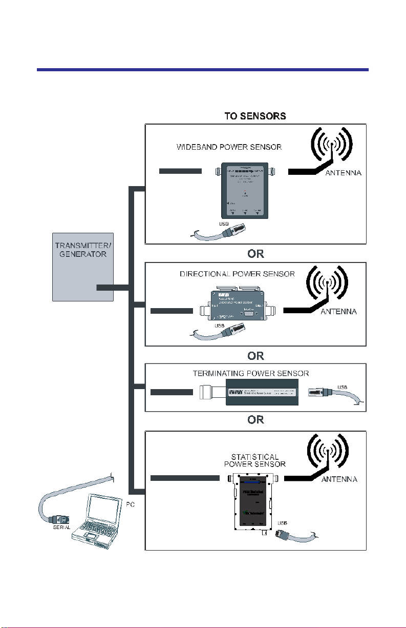
Power measurements verify and monitor the condition of a transmitter system.
To measure transmitter power, connect an external power sensor to the PC then
start the Virtual Power Meter program. Power sensors that are compatible with
the VPM are the Bird 5012B, 5014, 5015, 5015-EF, 5016B, 5017B, 5018B, 5019B,
7020, and STAT power sensors.
Note: ONLY sensors that have USB connections can be used with
VPM3 software.
The Power Meter mode has the following features:
Three display formats: numerical readout, analog dial, and chart
recording.
Display forward power, reflected power, match efficiency, peak power,
burst, and crest factor depending upon the capabilities of the sensor.
Display power measurements in Watts or dBm.
Display match units in either VSWR, Return Loss, Rho, or % Match effi-
ciency.
Adjust power and match readings for effects of attenuators, couplers,
and cable loss
Log data to a file and review
Save and recall sensor configuration setups
1
Page 10
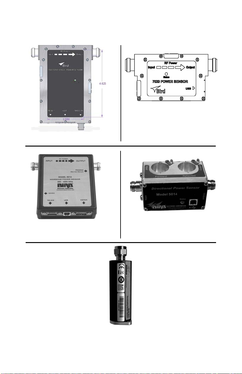
Figure 1 VPM Compatible Sensors
7022 Statistical Power Sensor (STAT)
7020 Power Sensor (WPS)
Directional Power Sensor
Wide Band Power Sensor
(WPS)
Terminating Power Sensor (TPS)
(DPS)
2
Page 11
Chapter 2 Set Up
Installing the VPM
1. Insert installation CD.
2. Select Install Software when prompted.
Note: Set-up will inspect the computer for any missing operating system prerequisites. If all are present, skip to step 6.
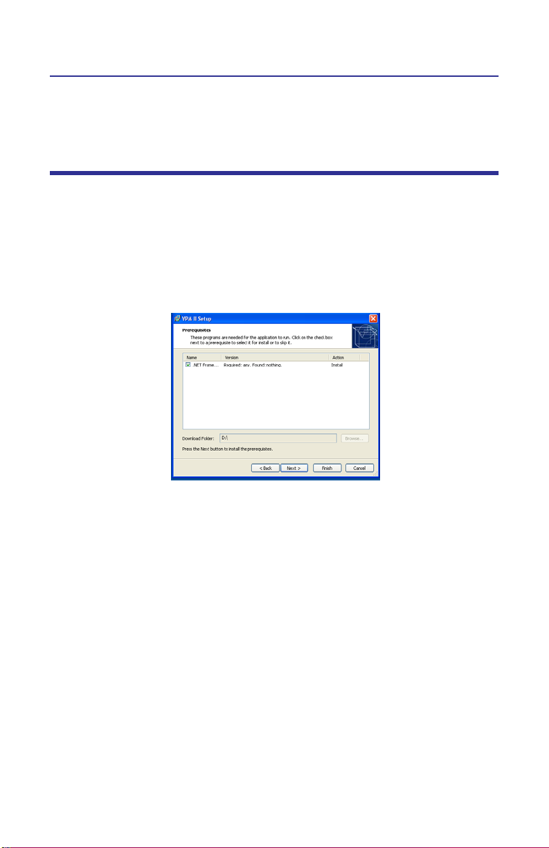
3. Select ‘Next ‘and the install utility begins the Prerequisites Installation process.
Figure 2 Install, Prerequisites Installation
4. Review the End-User License Agreement, check “I accept the terms of the
License Agreement” and select “Install.”
Note: The install Utility will install the prerequisites. This may take
several minutes
Note: When completed, check with Microsoft® support center for
any security updates. Typically, if “Automatic Updates” are configured
on the host PC, these will be automatically flagged and selected for
download and installation.
Note: The VPM3 installation utility will launch after the OS prerequisites are installed.
5. Do one of the following:
Accept the default installation location
Select a different folder:
6. Select ‘Next’ and the installer will complete.
7. Select “Finish” to launch the VPM3 program:
Note: When the VPM3 loads for the first time, the Preferences Dialog will prompt for a default log file save location. Perform the following to complete the process.
3
Page 12

8. Select the ‘Logging’ tab.
9. Enter a folder local to the PC to store log file data.
Note: This can be changed at any time in the Preferences. All active
sensor sessions must be closed before Preferences Dialog can be
opened.
10. Select the Advanced Tab.
11. Select the language in the drop down menu.
Note: For Mandarin Chinese, the East Asian languages files must be
installed. See “Language” on page 4.
Note: For any non-US English language setting, select ‘Windows’.
Any standard formats such as number and date formats from
"Regional and Language Options" found in the
Windows Control Panel will be mimicked in the VPM3 interface.
Preferences
The Preferences window will open automatically upon the first use of the VPM3.
If Preferences need to be changed at another time, it can be accessed from the
File drop down menu.
Default Settings may be restored when the Restore Default Settings button is
pressed.
General
Automatically connect to sensor on startup
When selected, the VPM3 will connect to the sensor upon the launching of the
program.
List sensors on startup
When selected, the VPM3 will list all available connectible sensors.
Display menu bar icons
When selected, the VPM3 will display the menu bar icons.
Language
Note: Default is English (US). For Chinese, the ‘East Asian languages’
files must be installed.
Installing Language Files
1. Open Control Panel>Regional>Language Options
2. Click on the Languages tab
3. Click on Supplemental language support.
4
Page 13

4. Click the ‘Install files for East Asian languages’ button.
5. Follow prompts.
Note: For any language change the application, must be restarted.
Note: All active sensor sessions must be closed before Preferences
Dialog can be opened.
Clear Message Box State
When this button is pressed, the Message will delete all store messages.
Figure 3 Preferences, General
File Locations
Note: Unless changed, the default directories are located in
Documents\VPM3 directory.
Session Directory
Sets the location of the session directory. See Save As on ......
Preset Directory
Sets the location of the preset directory. See Preset on ......
Measurement Data Directory
Sets the location of the data directory. See Measurements on .....
Figure 4 Preferences, File Locations
5
Page 14

Advanced
Chart History (points)
Sets the number of points to be collected in a session.
Playback History (frames)
Sets the number of frames created during a session.
Figure 5 Preferences, Advanced
6
Page 15
Connecting a Sensor
Note: Refer to the individual power sensor manual for specific infor-
mation regarding its sensor connections.
7
Page 16
1. Connect a power sensor to the computers USB port with a USB cable.
Note: Bird USB sensors are HID compliant devices and do not require
any driver installation. The only exception is the 7022 STAT power sensor which requires an installed driver.
Note: The 5014 and 5015 sensors LED will illuminate continually
when properly recognized by the host PC.
Note: The 5012B, 5016B, 5017B, 5018B, and 5019B sensors LED will
blink when properly recognized by the host PC.
2. Launch the VPM3.
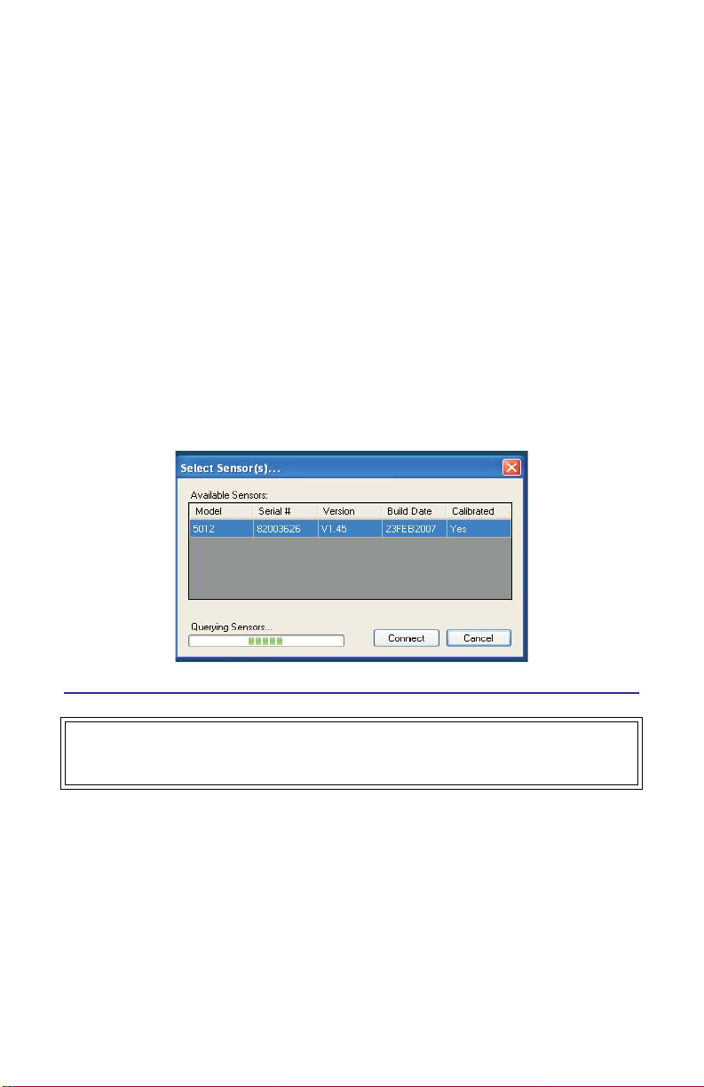
3. Select the sensor from the sensor connection manager.
4. Press the Configure menu key, after VPM3 acquires the power sensor, See “Configure” on page 22.
Note: Multiple sensors can be connected and/or monitored simultaneously through multiple USB ports or via a powered USB hub. It can
take up to 30 seconds to detect a sensor.
Figure 6 Sensor Connection Manager
Connecting the Directional Power Sensor (DPS)
WARNING
RF voltage may be present in RF element socket. Keep element in socket during
operation.
1. Connect the Bird DPS to the a USB port on the PC using the sensor cable
provided.
2. Connect the DPS to the RF line so that the arrow on the sensor points
towards the load.
Note: The arrow on the forward element should point towards the load.
Note: The arrow on the reflected element should point towards the
source.
Note: Both elements must be either APM/DPM or 43 types, do not
mix elements.
3. Set the power on the DPM to the forward element’s power rating.
8
Page 17
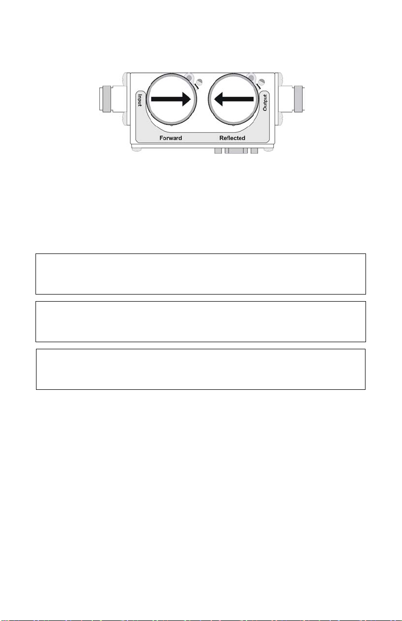
Figure 7 DPS Element Orientation
Connecting the Wideband Power Sensor (WPS)
1. Connect the Bird WPS to the a USB port on the PC using the sensor cable
provided.
2. Connect the WPS to the RF line so that the arrow on the sensor points
towards the load.
Connecting the Terminating Power Sensor (TPS)
CAUTION
Discharge all static potentials before connecting the TPS(-EF). Electrostatic
shock could damage the sensor.
CAUTION
When connecting the TPS or the TPS-EF, only turn the connector nut. Damage
may occur if torque is applied to the sensor body.
CAUTION
Do not exceed 2 W average or 125 W peak power for 5 μs when using the TPS
or the TPS-EF. Doing so will render the sensor inoperative.
Note: Connections are the same for the Bird 5011 and 5011-EF.
1. Connect the Bird TPS to the a USB port on the PC using the sensor cable
provided.
Note: An attenuator or directional coupler should be used with the
TPS in most applications.
Example - For an RF source with output between 0.1 and 50 W, use
a 40 dB, 50 W attenuator.
2. Connect the TPS RF input to the source (using an attenuator, if appropriate).
Note: Only connect the TPS directly to a source if the RF power will
be less than 10 mW.
Connecting the Statistical Power Sensor (SPS)
1. Connect the Bird WPS to the a USB port on the PC using the sensor cable
provided.
2. Connect the WPS to the RF line so that the arrow on the sensor points
towards the load.
9
Page 18

10
Page 19

Chapter 3 Average Power Mode
Display Types
Typical functions are selecting the type of measurement, type of element, units
of measure, measurement scales, offset values, and zeroing the sensor.
When a power sensor is properly connected (and detected), a status message,
located at the top of the Power Meter screen, will indicate the model number of
the power sensor (i.e., Bird model number). A popup with all decimals in the
reading will display when a mouse icon hovers over the specific reading.
Power Display
The selected measurement type is displayed in the main power display and
ancillary readings are displayed under the bar graph.
Bar Graph
The bar graph gives a visual indication of the main reading as well as displaying
the preset limits for the currently selected measurement. The scale of the graph
can be set to auto or full-scale.
Limit Indicators
'Virtual LEDs' indicate when pre-set limits have been exceeded.
Sensor Details
Provides a comprehensive display of all readings provided by the
sensor as well as all relevant configuration parameters
Sensor Status
Indicates the sensors connection status and zeroing progress.
11
Page 20

Figure 8 VPM Screen, Power Display
1
8
7
6
4
5
Item Description
1 Model of connected power sensor
2 Softkey Labels
3 Display Type
4 Menu Label Keys
5 Sensor Status
6 Sensor Readings
7 Power Meter
8 Limit Indicators
2
3
12
Page 21

Meter Display
Provides for a more traditional, analog-style view of main power display. The
selected measurement type is displayed in the analog meter as well as the preset limits for the currently selected measurement. The scale of the graph can be
set to auto or full-scale.
Sensor Readings
Numerical readout of selected measurement type and ancillary readings is displayed under the meter display.
Red indicates a questionable measurement. This means that the sensor has
determined that the measurement cannot be made or corrected reliably.
Figure 9 VPM Screen, Meter Display
Item Description
1 Model of connected power sensor
2 Softkey Labels
3 Display Type
4 Menu Label Keys
5 Sensor Status
6 Sensor Readings
7 Power Meter
8 Limit Indicators
13
Page 22

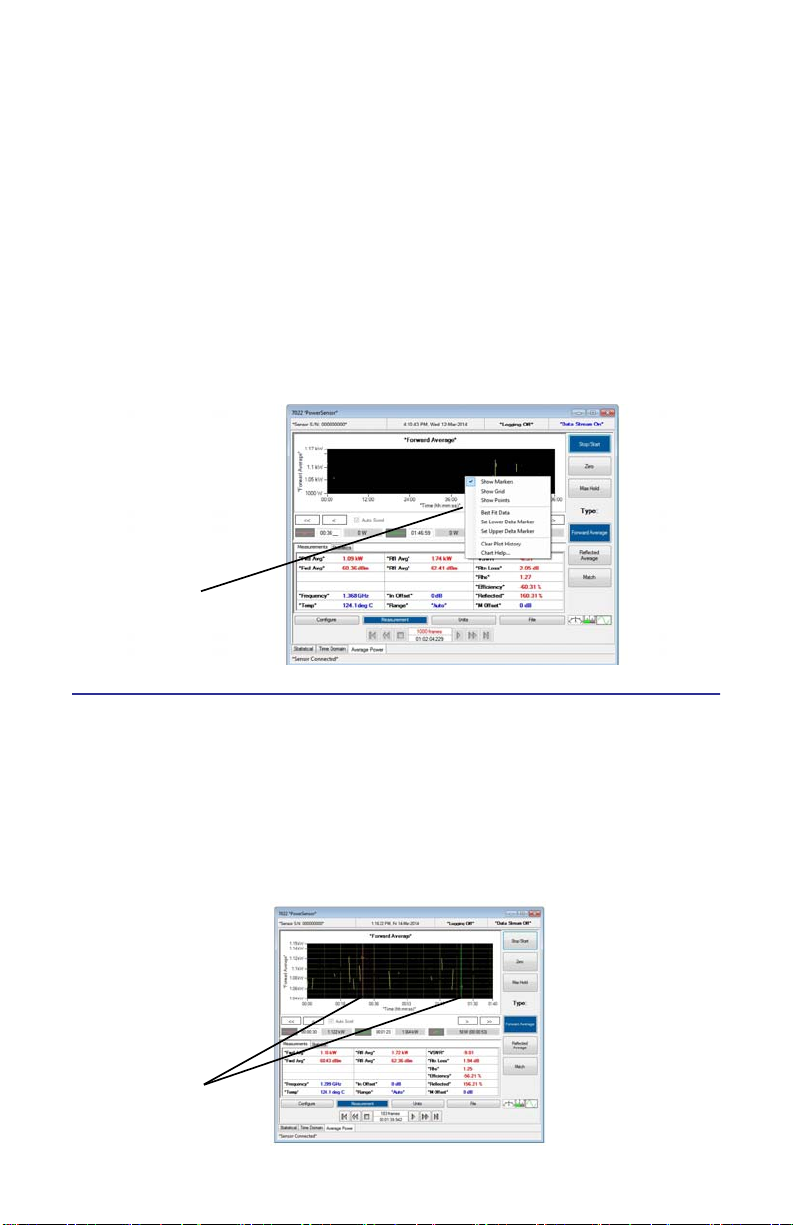
Chart Display
Used to display running time trace of all data collected by a sensor session or to
review data saved to a log file.
Note: Displaying the running time trace does not automatically save
data to a file. The Logging function must be activated to save data. See
“Logging” on page 30.
Figure 10 VPM, Chart Display
Item Description
1 Model of connected power sensor
2 Softkey Labels
3 Display Type
4 Menu Label Keys
5 Sensor Status
6 Sensor Readings
7 Marker Readout
8 Time Chart Display
9 Scroll Buttons
Note: Only data stored in Extensive Markup Language format (.xml) can
be recalled using the VPM3. See “Logging” on page 30.
Both Type and Units may be changed at any time in chart display.
Right clicking in chart will change display options:
14
Page 23
Show Markers
Toggles markers on & off. See “Markers” on page 15.
Show Grid
Turns major & minor grid on/off
Show Points
Toggles points on each data location
Best Fit Data
Adjust scales to show entire range of data
Set Lower/Upper Delta Marker
Moves the marker to the location of the mouse pointer & automatically sets the
position in time for the marker.
Figure 11 Chart Display, Options Menu
Options Menu
Markers
Click on marker & slide, also can type time in display to move markers to exact
time location.
Markers always stay in their current time reading.
Note: If the chart moves the markers off-screen, simply select ‘Set
Upper or Lower Delta Marker’ to return the markers to the current displayed time interval.
Figure 12 Chart Display, Markers
Markers
15
Page 24

Axis Scaling
Right click on Y or X axis to change scale from Auto to user-defined.
Figure 13 Chart Display, Changing Scale
Manual Axis Scaling
Change Time axis to ‘Manual’ allows scroll keys to be activated
<< , >> - Moves chart to start, end of log
< , > - Moves chart one span to the left or right
Auto Scroll - When checked, the chart will automatically advance
forward in time maintaining the same interval specified in the manual scale
entry.
Figure 14 Chart Display, Manual Axis Scaling
16
Page 25

Menu Bar
File
New Sensor Session
Displays sensor list and connection status dialog. Does not close the active sensor window/connection.
Open
Session - Displays the session open file dialog.
Preset - Displays the preset open file dialog.
Measurement - Displays the measurement open file dialog.
Reference Measurement - Displays the measurement open file dialog.
Close Session
Closes the active session window.
Save Session
Saves the active session without displaying the session file save dialog.
Save Session As...
Saves the selected session under a different name or file type.
Save Measurement Snapshot
Saves the most recent measurement frame to a file without displaying the measurement file save dialog.
Save Measurement Snapshot As...
Displays the measurement file save dialog.Recall/Review Log File...
Save Preset As...
Displays the preset file save dialog.
Recent Sessions
Displays the following submenu as a list of recent files
Recent Measurements
Displays the following submenu as a list of recent files
Preferences...
Sets the location of a saved files directory.
Exit
Closes the program and all open sessions.
17
Page 26

Mode
Note: The Mode menu is only displayed if the sensor supports more
than one measurement mode. For the 7022 sensor the following is displayed.
Statistical
Switch to Statistical mode. See “Statistical Power Mode” on page 37
Note: The mode tab will update to reflect this.
Time Domain
Switch to Time Domain mode. See “Time Domain Mode” on page 33.
Note: The mode tab will update to reflect this.
Average Power
Switch to Average Power mode. See “Average Power Mode” on page 11.
Note: The mode tab will update to reflect this.
Configure
Note: This menu will change depending on the sensor being displayed.
Input Offset
To read the true power when using a coupler or attenuator, enter (in dB) the
attenuation or coupling factor. To convert percentages to dB, use the equation:
Attenuation dB 10 Log10 Attenuation percent100=
Note: The Bird 5015-EF uses frequency-dependent correction factors
to provide more accurate measurements that are entered here. For
more information, refer to the owners manual for the 5015-EF.
Match Offset
The masking effect of cable loss can cause significant error when measuring
antenna VSWR or return loss levels. This masking can make an antenna to
“appear” to perform more efficiently than is actually the case. The offset error
may be corrected with the following equation:
RL at Antenna = RL at Transmitter - (2 x CL)
RL = Return Loss
CL = Cable Loss or Match Offset.
In the Match Offset dialog, enter the total insertion loss of the cable connected
between the power sensor and antenna, in dB. The VPM3 will correct the displayed match values according this equation.
18
Page 27

Smoothing
Note: The smoothing in this menu item is available only with the
7022 and is performed in the sensor itself. It only effects the average
power measurement in the forward direction and is used for very low
rep rate signals (<200Hz).
Selects smoothing that is performed by the sensor for average forward and
reflected power.
None - No smoothing is performed.
Low - Uses a moving average of 8 samples.
Medium - Uses a moving average of 16 samples.
High - Uses a modified moving average (exponential average with alpha = 1/N).
Frequency Setpoint
Note: 7022 Only.
Auto - The frequency will be determined by the sensor.
Full - The specified frequency will be used in correcting the power measurement.
Note: Use this when the sensor is unable to measure the frequency
of a signal.
Duty Cycle
Note: 7022 Only.
Sets the duty of a measurement for determining the Burst Average power. If sensor is capable, the duty cycle will be inferred by the sensor hardware and
reported. A user-defined duty cycle can be entered to override the sensor provided value.
Note: If zero is entered, the duty cycle automatically sets to Auto.
Note: For best duty cycle measurement with the 7022, have at least
10 pulses on the time domain screen.
Auto - The duty cycle will be determined by the sensor.
Specify Duty Cycle - The specified duty cycle will be used to determine the
Burst Average power.
Note: Use this for best accuracy when the duty cycle is known.
See “Specifications” on page 51 for more information on how duty cycle is calculated and used for each sensor that has the feature.
Measurement
Type
Selects the parameter that is displayed in the bar graph, meter or chart.
19
Page 28
Units
Power - Toggles the power measurement between Watts and Decibels.
Match - Allows selection of match measurement units.
Note: This is dependent on the sensor attached.
Start Acquisition
Starts a trace for the selected session.
Stop Acquisition
Holds a trace until a started again.
Max Hold
Holds and displays the highest trace data points.
Zero
Performs a zero calibraion on the selected sensor. See “Zeroing a Sensor” on
page 32.
Log
Enable Data Logging
Starts monitoring the selected Measurement type. See “Logging” on page 30.
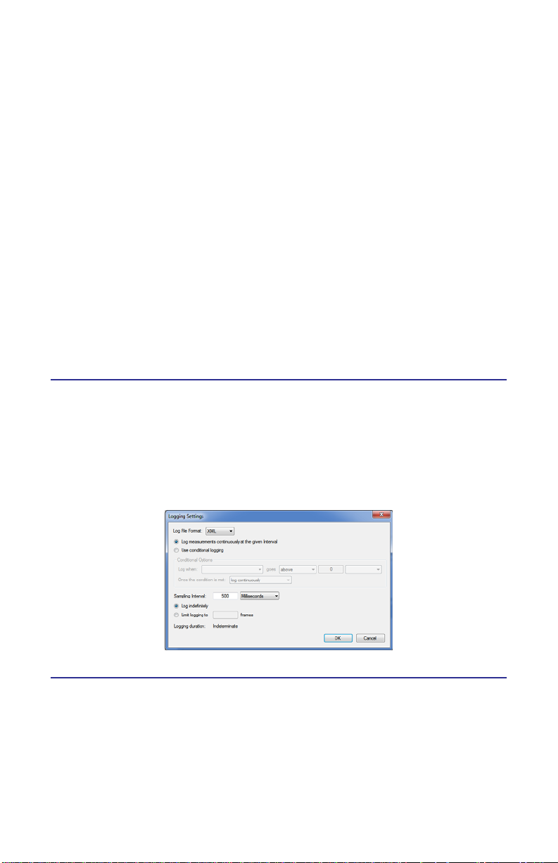
Logging Settings
See “Logging” on page 30.
Figure 15 VPM, Logging Settings
View
Control Panel
When selected, it will display the control buttons.
Playback Controls
When selected, it will display the playback controls.
20
Page 29

Details
When selected, it will display the details of the measurement.
Fullscreen Mode
Toggles the display to full screen on and off.
Display Style
Choose between three:
Digital
Analog
Chart
Meter Range
Choose between two:
Auto
Full
Smoothing
Choose between two:
Enabled
Specify Number of Readings
Playback
Choose between six:
Clear Buffer
No Delay
1 sec
2 sec
4 sec
8 sec
Window
Cascade Sessions
Organizes the sessions in a cascading, offset display.
Tile Sessions Horizontally
Organizes the sessions horizontally.
Tile Sessions Vertically
Organizes the sessions vertically.
21
Page 30

Help
User Manual
Opens a html version of the user manual.
About Virtual Power Meter
Displays version info about the VPM and any attached sensors.
About Sensor
Displays model information of the selected sensor.
Menu Label Keys
Configure
Note: Specific configuration features depend upon the power sensor
being used.
When the Configure menu key is pressed, the soft key functions that specify the
setup information about the sensor and the measurements are enabled. What
type of element in the power sensor, offsets for input and match, duty cycle,
and the scale for forward and reflected power is displayed at this time.
Note: For DPS sensors, element scales have pre-defined values and
an “Other” category for arbitrary values.
Note: The 5015-EF offset factors are used for frequencies above 4
GHz.
For Wide Band Power Sensors
Video Filter - Except for average power and VSWR measurements, all WPS
measurements rely on a variable video filter to improve accuracy. This filter can
be set to either 4.5 kHz, 400 kHz, or full bandwidth. It should be as narrow as
possible while still being larger than the demodulated signal bandwidth (video
bandwidth). Narrowing the filter limits the noise contribution caused by interfering signals. Listed below are some common modulation schemes and the
appropriate video filter.
Video Filter Modulation Type
4.5 kHz CW Burst (Burst width > 150 μs), Voice Band AM, FM, Phase
Modulation, Tetra
400 kHz CW Burst (b.w. > 3 μs), GSM, 50 kHz AM, DQPSK
Full Bandwidth CW Burst (b.w. > 200 ns), CDMA, WCDMA, DQPSK, DAB/DVB-T
Note: 7022 has 5KHz, 500KHz, and 5MHz VBW filter and only effects
the time domain data, not average power.
Figure 16 Video Filter Settings, 300 kHz Signal
22
Page 31

1. Press the Input Offset soft key and use the key pad to enter the amount of
attenuation then press the Enter key.
2. Press the soft key to select Auto Duty Cycle.
3. Press the soft key to select Auto Range.
Figure 17 VPM, Configure, WPS
For Sensor 5015 and 5015-EF
1. Press the Power: Watts soft key.
2. Press the Input Offset soft key and use the key pad to enter the amount of
attenuation then press the Enter key.
23
Page 32

Figure 18 VPM, Configure, TPS
For Sensor 5014
43 Peak - Refer to the 5014 owner’s manual.
DPM - Refer to the 5014 owner’s manual.
1. Press the soft key to select the type of element.
2. Press the Forward Scale to enter the watt rating of the forward element.
3. Press the F/R Scale 10:1 Ratio soft key to select ON.
4. Press the Input Offset soft key and use the key pad to enter the amount of
attenuation then press the Enter key.
Figure 19 VPM, Configure, DPS
For Statistical Senors
Input Offset - See “Input Offset” on page 18.
Match Offset - See “Match Offset” on page 18.
Meter Range - .
Smoothing - See “Smoothing” on page 19.
Freq Setpoint - See “Frequency Setpoint” on page 19.
Duty Cycle - See “Duty Cycle” on page 19.
24
Page 33

Measurement
Note: Specific measurement types depend upon the power sensor
being used.
Figure 20 VPM, Type, WPS
Figure 21 VPM, Type, DPS
Forward and Reflected Power
Average power is a measure of the equivalent “heating” power of a signal, as
measured with a calorimeter. It measures the total RF power in the system, and
does not depend on number of carriers or modulation scheme.
Average power is the most important measurement of any transmission system
since the average power is normally specified on the operating license. It is also
valuable as a maintenance tool, showing overall system health, and for calibration.
25
Page 34

Match
p
Match measures the relation between forward and reflected average power.
The health of the feedline and antenna systems can be monitored using Match,
or VSWR, measurement under full power operating conditions. High VSWR is an
indicator of feed line damage, overtightened cable or feed line clamps, or
antenna changes/damage due to weather conditions, icing, or structural damage to the tower.
Rho and Return Loss are also the same measurement, but in different units:
Rho -
VSWR -
Return Loss (dB) -
Rho PRPF=
VSWR
1 p+
------------ -=
1
–
ReturnLoss dB20 log=
Figure 22 Average and Peak Envelope Power, Square Wave Signal
Forward Peak Power
Peak power measurements detect amplitude changes as a signal modulates the
carrier envelope.
Transmitter overdrive can be detected with peak measurements. Common
problems are overshoot at the beginning of burst packets, amplitude modulation, and excessive transients. These damage system components with excessive peak power and also cause data degradation, increasing the Bit Error Rate.
For TDMA applications, Peak and Burst Power measurements are used to detect
overshoot in single timeslots. Other timeslots must be turned off for this test.
Peak Average Power
This displays the average of the positive and negative peak power readings.
Burst Average Power
Burst width (BW) is the duration of a pulse. Period (P) is the time from the start
of one pulse to the start of the next pulse. Duty cycle (D) is the percentage of
time that the transmitter is on. To calculate the duty cycle simply divide the
burst width by the period (D = BW / P). Low duty cycles mean that the burst
width is much less than the period; a large amount of dead time surrounds each
burst. For low duty cycles, the burst average power will be much larger than the
average power.
After peak power is measured, a threshold of ½ the peak is set. The sampled
power crosses that threshold at the beginning and end of each burst. The time
between crossings is used to calculate the duty cycle. Burst Average Power is
calculated by dividing the Average Power by the Duty Cycle.
26
Page 35

Burst average power is calculated in the 7022 automatically using the average
detector and the duty cycle.
Burst average power can also be calculated in the time domain mode using the
average power between markers function.
Burst power measurements provide accurate, stable measurements in bursting
applications such as TDMA and radar. Accurately measuring the output signal
strength is essential for optimizing radar coverage patterns. Actual transmitted
power in a single timeslot can be deter-mined in TDMA. The other timeslots
must be off during this test.
Figure 23 Burst Average Power
Crest Factor
Crest factor (CF) is the ratio of the peak and average powers, in dB. The WPS calculates the Crest Factor from the Forward Peak and Average Power measurements.
Crest factor is becoming one of the most important measurements as communication systems move into the digital age. For CDMA and similar modulation
types the CF may reach 10 dB. If the crest factor is too large, the transmitter will
not be able to handle the peak powers and amplitude distortion will occur. Crest
factor can also detect overdrive and overshoot problems. Knowing the CF allows
end-users to more accurately set base station power and lower operating costs.
Figure 24 Crest Factor, 10 dB CDMA Signal, 100 W Peak, 10 W Ave
Complementary Cumulative Distribution Function (CCDF)
CCDF measures the amount of time the power is above a threshold. This threshold is set in the Configure, CCDF Factor menu. Equivalently, it is the probability
that any single measurement will be above the threshold. The WPS samples the
power over a 300 ms window and compares it to a user-specified threshold, in
Watts. The time above the threshold relative to the total time is the CCDF.
27
Page 36

CCDF measurements are most useful for pseudo-random signals, such as
WCDMA, where a high CCDF means that the transmitter is being overdriven.
CCDF can also detect amplitude distortion within an envelope caused by
unwanted modulating signals. In TDMA systems, CCDF indicates the health of
power amplifier stages and their ability to sustain rated power over an appropriate timeframe. As a trouble-shooting aid, CCDF allows tracking of trends such as
amplifier overdrive (which can cause dropped calls and high bit error rates).
Figure 25 CCDF, 100 W Signal, 80 W Threshold, 20% CCDF
Units
When the Units menu key is pressed, the soft key functions that select the units
of measure are enabled. For power measurements, Watts or dBm can be
selected. For match measurements, VSWR, dB, rho, and percent (%) can be
selected.
Figure 26 VPM, Units, WPS
28
Page 37

Figure 27 VPM, Units, TPS
Figure 28 VPM, Units, DPS
File
Note: Save and Save As captures the most recent measurement
readings. It will not store the time-chart information. To store time
chart display, ensure logging is enabled. See “Logging” on page 30.
Save
Press this soft key to create a snapshot of the readings displayed on the screen.
That snapshot is saved in the log file folder “Setup” in the Preferences under the
File menu item. Each quick save is stored in a separate file that is named using
the date-time file naming format:
MMMM_NNNNNNNN_YYYYMMDD_HHMMSS.xml
Model
Serial Number
Year
Month
Day
Hour
Seconds
Minute
29
Page 38

Save As
Same as Quick Save, only the program will request a title to save the trace under.
Figure 29 VPM, File
Enable
Enable Logging
See “Logging” on page 30.
Logging Settings
See “Logging” on page 30.
Open Preset
Applies a preset to the measurement.
Logging
Measurement logging is a powerful tool for monitoring and tracking system performance. Storing the readings enables the ability to graph the output over time, know
the exact time of a failure, or compare systems.
The VPM3 can be set up to take many readings over a short test period, to take
a few readings a day for long-term monitoring, to log only while the transmitter
is on, or to log when power spikes or drops below a critical value, depending on
specific needs. To begin logging:
1. Configure the logging options.
2. Begin logging by selecting Enable Logging.
Note: When logging is active, in the upper right of the sensor session
will display “Logging On.”
3. Stop logging by selecting Enable Logging.
After logging is complete, the data can be reviewed in the a VPM3 logfile recall/
review session or imported into Microsoft Excel or another spreadsheet program for analysis.
Note: Log files are stored in the default log file directory under
:Documents/VPM3/Measurements.
30
Page 39

Analyzing Logged Data
The simplest way to view logged data is to recall in VPM3. See “Chart Display”
on page 14.
Note: Only log files saved as .xml can be opened and viewed in the
VPM3. Files saved in comma-separated format (CSV) can be read by
most common spreadsheet programs.
Since logged data is stored in a text file in an .xml or comma-separated text file
where each line is one data record. Fields are separated by commas format, it is
also readable by most spreadsheet programs.
Each log file is stored in a separate file that is named using the same date-time
file naming format as for quick-save.
Opening .xml Files in Excel
1. Open the file in Microsoft Excel.
Note: The file will appear in Microsoft Excel with each field in its own
column.
2. Filter the data, since the Extensive Markup Language format is a hierarchical format.
a. In the Measurement column, select the drop-down and check only
the Forward Average label.
b. In the Limit Type column, select the drop-down and check only the
Lower label.
Note: This will now show data in a time vs. power format. Additional
filtering and sorting can be applied using the options in the column
headers.
Opening .csv Files in Excel
1. Open the file in Microsoft Excel.
Note: The file will appear in Microsoft Excel with each field in its own
column. If all the data is in a single column, follow these steps to convert it:
a.Click on the column name, to select the entire column.
b.Select Text To Columns, under the Data tab.
Note: A conversion wizard should open.
c.Select Delimited, under Original Data Type.
d.Click Next.
e.Check Comma, under Delimiters.
Note: All other delimiters should be unchecked. Treat Consecutive
Delimiters as One should be unchecked.
f.Click Next.
g.Click Finish.
31
Page 40

2. Create a graph of the forward and reflected average power as a function of
time:
a. Select row 1 by clicking on the row name.
b. Select Delete, under the Edit tab.
Note: The first line of header information will be deleted.
c. Click on cell B1.
d. While holding down the Ctrl key, select columns B (Time), H (Avg
Fwd W), and J (Avg Rfl W).
e. Select Chart, under the Insert tab.
Note: The chart wizard should open.
f. Select XY (Scatter).
g. Select the Line subtype.
h. Click Next.
i. Click Next in the data range, which should already be set.
j. Enter a title and names for the X and Y axes.
k. Click Finish.
Note: Other data can be graphed by selecting the appropriate columns in step d.
Zeroing a Sensor
1. Check that no RF is in the system.
Note: The sensor will read “~0.”
2. Do one of the following:
Press the Measurement menu button.
Go to the Measurement menu and select the Zero menu item.
Note: Calibration will take about 40 seconds. Do not interrupt the
calibration. A progress bar for the calibration will be displayed on the
screen.
Note: Some soft key features will not be available for certain power
sensors.
3. Press “Run” to resume data collection with the new Zero offset.
Figure 30 Zeroing Sensor
32
Page 41

Chapter 4 Time Domain Mode
Display
Figure 31 Screen Features, Time Domain
Item Description
1 Model of connected power sensor
2 Lower Delta Marker
3 Upper Delta Marker
4 Menu Label Keys
5 Sensor Status
6 Modes
7 Hard Key Menu
8 Limit Indicators/Statistic Indicators
9 Marker Indicators
10 Time Domain Plot
33
Page 42

Menu Bar
File
See “File” on page 17.
Mode
See “Mode” on page 18.
Configure
Note: This menu will change depending on the sensor being displayed.
Input Offset
To read the true power when using a coupler or attenuator, enter (in dB) the
attenuation or coupling factor. To convert percentages to dB, use the equation:
Attenuation dB 10 Log10 Attenuation percent100=
Note: The Bird 5015-EF uses frequency-dependent correction factors
to provide more accurate measurements that are entered here. For
more information, refer to the owners manual for the 5015-EF.
Scale
There are three settings for the measurement plot.
Time (Horizontal)
Power (Vertical)
Reference Level
Bandwidth
There are four settings to choose from:
No Filter
5 kHz
5 MHz
20 MHz
34
Page 43

Frequency Setpoint
See “Frequency Setpoint” on page 19.
Duty Cycle
See “Duty Cycle” on page 19.
Measurement
Start Acquisition
Starts a trace for the selected session.
Stop Acquisition
Holds a trace until a started again.
Enable Pulse Measurement
Starts a pulse trace for the selected session.
Zero
See “Zeroing a Sensor” on page 32.
Trigger
Source
Choose between three:
Internal - Triggered when the signal crosses the specified trigger level.
External - Triggered by a signal applied to the external trigger connector.
Manual - Triggered by selecting the manual trigger menu selection or
button.
Mode
The mode affects operation only when the selected source is Internal or External.
Choose between three:
Single - Once the trigger occurs the signal is displayed. No further trig-
ger events are acted upon until you stop and restart the measurement
Auto - The measurement is triggered automatically if the specified trig-
ger event does not occur within the greater of 10ms or the acquisition
interval of the last measurement.
Normal - The measurement is not triggered until the specified trigger
event occurs.
35
Page 44

Edge
When the selected source is Internal, this selects the direction that the signal
crosses the specified trigger level to cause a trigger event.
Choose between two:
Rising
Falling
Level...
Note: Auto level was added that sets the trigger level automatically
half way between the max and min values of the previous time
domain data set.
Sets a specific the trigger power level when the source is internal.
Delay...
Specifies the delay between the trigger event and the start of the signal acquisition.
0 - the trigger event occurs at the mid-point of the time axis.
Positive values - Trigger event shifts to the left on the display.
Negative values - Trigger event shifts to the right on the display.
Note: Values are limited by the sensor. If a value exceeding a limit is
specified, the sensor will change that value to the limit.
Holdoff...
Specifies the minimum amount of time from the end of one measurement to
the next trigger event.
Manual Trigger
Triggers a single measurement.
Zero Delay
Resets any Trigger delay to zero.
Log
See “Logging” on page 30.
View
See “View” on page 20.
Window
See “Window” on page 21.
Help
See “Help” on page 22.
36
Page 45

Chapter 5 Statistical Power Mode
Most modern wireless communication systems employ complex modulation
and channel access methods like orthogonal frequency division multiplexing
(OFDM), or code division multiple access (CDMA). These methods use a combination of amplitude and phase modulation to create symbol based multichannel
or multicarrier systems that result in pseudorandom or noise-like power envelopes. The consequence is that modulation parameters such as AM depth or FM
modulation index are not useful. Indeed, the peak-to-average power ratio of
the modulated carrier is a complex function of the data stream content rather
than just amplitude, and as such is not constant with time. Since digitally modulated signals often appear noise-like it makes sense to use statistical analysis in
order to characterize them.
RF Power meters that provide measurements based upon statistical methods
have been available for use in laboratory environments for more than ten years.
The most significant advantage is that they are capable of making meaningful
power measurements of signals incorporating complex modulation methods. In
essence, provide meaningful measurements independent of the modulation
method used in the system.
The Bird Statistical Power Meter is a rugged, portable power sensor that is well
suited for use in the field by less sophisticated users than those that would typically be found in a laboratory setting.
37
Page 46

Display
Figure 32 Screen Features, Statistical Mode
Item Description
1 Model of connected power sensor
2 Lower Delta Marker
3 Upper Delta Marker
4 Menu Label Keys
5 Sensor Status
6 Modes
7 Hard Key Menu
8 Limit Indicators/Statistic Indicators
9 Marker Indicators
10 Time Domain Plot
38
Page 47

Statistical Power Measurement Methodology
Complementary Cumulative Distribution Function (CCDF)
The most commonly used parameter is that of the Complementary Cumulative
Distribution Function (CCDF), which provides an indication as to the probability
that the measured power level is greater than a specific power value. This technique has become extremely useful with modern communications systems,
where power levels appear to be noise-like, and do not follow a traditional
power envelope. With regard to CCDF, it is important to understand that CCDF
measurements require no time synchronization with the waveform to be measured, and no specific test signal is required. This type of power analysis may be
performed using live, “on-air” signals.
Example - 9 Channel CMA, One Signal
This figure illustrates a time record for a nine channel CDMA One Signal. Note the
noise-like nature of the signal, and the lack of any defined waveform envelope.
This figure illustrates the same signal using statistical methods (CCDF), where
the Y axis represents the percentage of time that the signal is at or above a level
specified by the X axis, and the X axis represents the level (dB) of the signal
above the average power of the waveform.
In this case, the signal of interest is being compared to band limited Gaussian
noise, as this signal has a defined characteristic, dependent upon the signal
bandwidth.
Example - LTE vs Gaussian Noise
This example illustrates another view of this concept, comparing the statistical
performance of a live LTE envelope compared to Gaussian noise.
Figure 41 presents another view of this data in numeric format, as a means of
illustrating a few of the data points on the CCDF curves. This table shows that
10% of the time, this particular LTE waveform demonstrates a peak to average
ratio of 4.46 dB. At the same time, the table also reveals that the same waveform demonstrates a peak to average ratio of 10.56 dB 0.0001% of the time.
Interpreting Statistical Data
There are many factors that influence the performance of modern communications systems. Some examples:
The presence of interfering signals within the operating bandwidth of
the system.
Transmission line discontinuities resulting in multiple reflections within
the transmission system.
39
Page 48

Poor amplifier linearity caused by amplifier compression. This results in
signal distortion and poor fidelity of transmitted waveforms.
Antenna damage or degradation resulting in high transmission system
reflections.
Issues with transmitter modulator performance resulting in high error
vector magnitude (EVM).
Many of the above transmission system issues may be identified through the
use of the statistical techniques mentioned above. For example, if a particular
LTE radio system was known to be dropping calls at a higher rate than expected,
a service technician will need to know whether the problem is with the radio
itself, or with some element of the transmission system, or with the air interface. Measuring the CCDF statistics of the base station radio, while terminated
with a high quality 50 ohm termination, and then again with the radio connected to the transmission and antenna system will provide clues as to where
the issues may be.
Another useful technique is to compare live data from the system with a known
“reference” transmission, as is demonstrated above using Gaussian waveforms.
40
Page 49

Menu Bar
File
See “File” on page 17.
Mode
See “Mode” on page 18.
Configure
Note: This menu will change depending on the sensor being displayed.
Scale
Specifies the maximum of the Upper Range.
Run Mode
There are two settings to choose from:
Normal - Takes one measurement and stops.
Clear Restart - Once a measurement has been completed and dis-
played another is started automatically.
Bandwidth
There are four settings to choose from:
No Filter
5 kHz
5 MHz
20 MHz
Confidence Factor
Sets the duration of the measurement.
Percentage - Acquires sufficient samples to achieve an error tolerance of +/-
0.1% with the specified confidence factor.
Number of Samples - Acquires at least the specified number of samples.
Time Duration - Acquires samples for at least the specified amount of time.
41
Page 50

Figure 33 Confidence Factor
Measurement
Start Acquisition
Starts a trace for the selected session.
Stop Acquisition
Holds a trace until a started again.
Show/Hide Reference
Sets the reference display.
Log
See “Logging” on page 30.
View
See “View” on page 20.
Window
See “Window” on page 21.
Help
See “Help” on page 22.
42
Page 51

Chapter 6 Power Sensors
Accuracy
The Bird power sensors are highly accurate. Accuracy is specified for each sensor
type is typically given as a percent of reading or of full-scale.
Example - If a sensor has a specified accuracy of 5% of reading +
1.0 uW, then for a 10 mW signal the uncertainty is ± 0.501 mW. For
a 1 mW signal the measurement uncertainty is ± 0.051 mW.
Sensor Uncertainty
While this value is a good estimate, the sensor is actually more accurate. The
sensor’s accuracy also depends on the temperature, and the power and frequency of the source; Table 1 lists some examples of uncertainty factors. If an
uncertainty is given as a power, divide this value by the measured RF power and
convert to a percentage. For example, an uncertainty of ± 0.25 μW with a RF
power of 10 μW is a 2.5% uncertainty. Table 2 lists external factors, such as
using attenuators or using a cable to connect a sensor to the transmitter, which
could affect the measurement uncertainty.
Table 1 - Example Uncertainty Factors
Error Source Conditions Uncertainty
Calibration Uncertainty ± 1.13%
Frequency Response 40 MHz to 4 GHz ± 3.42%
Temperature Linearity –10 to +50 °C ± 3.43%
*
Other
Resolution ± ½ smallest displayed digit
Zero Set
Noise
†
± 0.125 μW
†
*. Above 40 °C, when making measurements at frequencies
between 40 and 100 MHz, add 1.1%.
†. After a 5 minute warm-up, measured over a 5 minute
interval and 2 standard deviations
Table 2 - External Factors
< 40 °C or > 100 MHz ± 0.50%
(e.g. for a mW scale, three decimal places
are displayed. ½ the smallest is 0.5 μW)
above 1.05 mW ± 0.7 μW
105 μW to 1.05 mW ± 0.4 μW
below 105 μW ± 0.2 μW
Error Source Conditions
Attenuator Uncertainty Frequency dependent
Cable Uncertainty Frequency and length dependent (± 5% at
1 GHz for a ‘reasonable’ 1.5 m cable)
43
Page 52

The root sum square (RSS) uncertainty is the industry standard method for combining independent uncertainties. To determine the TPS's RSS uncertainty:
1. Square each uncertainty factor.
2. Add these values together.
3. Take the square root of this sum.
Table 3 has two examples of uncertainty calculations. The first is a 10 mW signal
at room temperature. The second is a 10 μW, 40 MHz signal at 50°C. Since this
measurement is at both low frequency and high temperature, the uncertainty
will be increased. Note that the RSS uncertainties are smaller than the values
from the rough estimate. This will always be the case.
Table 3 - Uncertainty Examples
Example 1
(10 mW, Room Temp)
Error
Source
Cal. Uncert. 1.13 % 1.28 1.13 % 1.28
Freq. Resp. 3.42 % 11.70 3.42 % 11.70
Temp. Lin. 3.43 % 11.76 3.43 % 11.76
Other 0.5 % 0.25 1.6 % 2.56
Res. 0.005 % 0.00 0.5 % 0.25
Zero Set 0.00125 % 0.00 1.25 % 1.56
Noise 0.007 % 0.00 2 % 4.00
Sum Uncert. 24.99 33.11
RSS Uncert. 5.00 % 5.75 %
Quick Uncert. 5.01 % 16 %
Percent
Uncert.
RSS
Term
Example 2
(10 μW, 40 MHz, 50°C)
Percent
Uncert.
RSS
Term
Mismatch Uncertainty
Another factor of measurement accuracy is mismatch uncertainty. When a source
and a load have different impedances, some signal will be reflected back to the
source. This uncertainty depends on both the VSWR of the TPS and the VSWR of the
rest of the system. For a system VSWR of 1.0, the mismatch uncertainty would be 0.
For a VSWR of 5.0, the mismatch uncertainty would be 12.5%. Given the VSWR of
the TPS and the source, the mismatch uncertainty can be calculated as follows.
Mismatch uncertainty (MU) is related to the reflection coefficient ( by the formula:
MU percent1
+21–100=
s1
Note: where s = reflection coefficient of the source,
and l = reflection coefficient of the load (the TPS)
The reflection coefficients can be calculated from the VSWR by the formula:
VSWR 1–VSWR 1+=
44
Page 53

Example - If a source with a 1.50:1 VSWR with the Terminating
Power Sensor was used, which has a max VSWR of 1.20:1, the mismatch uncertainty would be calculated as follows:
1.50 1–1.50 1+ 0.200==
s
1.20 1–1.20 1+ 0.091==
1
MU 1
0.200 0.091+
2
1–100 3.67==
If a source with a 1.30:1 VSWR was used instead, the mismatch uncertainty
would be:
1.30 1–1.30 1+ 0.130==
s
1.20 1–1.20 1+ 0.091==
1
MU 1 0.130 0.091+
2
1–100 2.39==
Using a lower VSWR source can drastically reduce the mismatch uncertainty.
Keep in mind that the typical VSWR of the Model 5011 is 1.03:1, which gives a
much lower mismatch uncertainty.
Example - With the 1.50:1 source, the mismatch uncertainty would
be:
1.50 1–1.50 1+ 0.200==
s
1.03 1–1.03 1+ 0.015==
1
MU 1
0.200 0.015+
2
1–100 0.59==
To determine the total uncertainty of the measurement, combine the RSS
uncertainty with the mismatch uncertainty using the RSS method. Square the
RSS uncertainty, add it to the square of the mismatch uncertainty, and take the
square root.
Using Example 1 in Table 3 with a source VSWR of 1.50 and a TPS VSWR of 1.20,
the total uncertainty would be:
5.0023.67
2
+ 6.20 percent=
For example 2, the total uncertainty would be 6.82 %.
45
Page 54

Directional Power Sensor (DPS) Measurements
Description
The DPS series sensors utilize elements in order to make power measurements.
Each element has an arrow on it that represents the direction in which it measures power. The elements ignore power in the opposite direction with a directivity of at least 25 dB. The DPS series can make power measurements using
either 43 type or APM/DPM elements, and the readings available vary, based on
which elements are being used.
Since the DPS uses two elements, it can measure the quality of the system by
comparing the forward and the reflected power. This is usually presented in the
form of VSWR (voltage standing wave ratio) or Return Loss.
43 Type Elements
The 43 type elements are normally used to measure peak power. These elements can measure the peak power of a system with an accuracy of +/-8% of full
scale as long as the signal meets the following requirements:
At least 15 pps (pulses per second)
Minimum pulse width of 15 μs
(800 ns if frequency is greater than 100 MHz)
Minimum Duty Cycle of 0.01%
In addition, 43 type elements can be used to measure average power in signals
with a peak-to-average ratio close to 1, like a CW or FM signals. In these cases,
the average power is measured with an accuracy of +/- 5% of full scale.
APM/DPM Elements
The APM/DPM elements are used to measure true average power. True average
power means the sensor provides equivalent heating power of the signal,
regardless of modulation or number of carriers. These elements can measure
average power with an accuracy of +/-5% of reading from full scale down to
2.5% of full scale.
Note: The equivalent heating power is dependent on the duty cycle
of a signal. If a system puts out 50 watts with a 50% duty cycle, the
APM/DPM elements will measure 25 watts.
46
Page 55

Terminating Power Sensor (TPS)
Description
The Bird Terminating Power Sensor (TPS) and 5015-EF extended frequency TPS
are a diode-based power sensors that measures true average power.
For best results, wait 5 minutes after applying power to the sensor before taking
readings.
Zeroing Sensor
Over time, the sensor’s “zero value” (reading with no applied RF power) can
drift, making all readings inaccurate by this value. For example, if the zero value
is –0.02 W, measuring a 50 W signal will give a reading of 49.98 W, a 0.04%
error. Measuring a 1 W signal will give a reading of 0.98 W, a 2% error. If the
drift would be a significant error, rezero the sensor:
1. Ensure the sensor has reached a stable operating temperature.
2. Ensure no RF power is applied to the sensor.
3. Press “Zero” to begin Calibration.
Note: Calibration will take about 40 seconds. Do not interrupt the
calibration! A bar on the screen will display calibration progress.
Correction Factors
The Bird TPS-EF uses frequency-dependent correction factors to improve its
accuracy. To use the correction factors:
1. Look at the Correction Factor Table on the side of the TPS and find the correction factor corresponding to the frequency under test.
2. Add the correction factor to all other necessary offsets (for example, the
coupling factor of a directional coupler).
3. Enter the total offset into the power meter.
4. Input the Offset on the VPM3. See “Input Offset” on page 18.
Note: Correction factors are only required above 4 GHz. Below
4 GHz, the TPS-EF can be used as a normal TPS. See “Terminating
Power Sensor (TPS)” on page 47.
47
Page 56

Wideband Power Sensor (WPS) Measurements
Note: WPS Firmware V1.45 or latter is required to operate on the
VPM3.
Description
The Bird Wideband Power Sensor (WPS) is a Thruline sensor that can measure
average, peak, or burst power, VSWR, crest factor, and Complementary Cumulative Distribution Function (CCDF).
Note: Firmware upgrades extending the WPS’s capabilities may be
periodically released. For the latest firmware upgrade, contact Bird
Customer Service at (866) 695-4569 or visit the Bird website at http://
www.bird-technologies.com (Mousing over http://www.bird-technologies.com shows a link to http://bird-electronic.com).
Zeroing Sensor
Over time, the sensor’s “zero value” (reading with no applied RF power) can
drift, making all readings inaccurate by this value. For example, if the zero value
is –0.02 W, measuring a 50 W signal will give a reading of 49.98 W, a 0.04%
error. Measuring a 1 W signal will give a reading of 0.98 W, a 2% error. If the
drift would be a significant error, rezero the sensor:
1. Ensure the sensor has reached a stable operating temperature.
2. Ensure no RF power is applied to the sensor.
3. Press “Zero” to begin Calibration. See “Zeroing a Sensor” on page 32.
48
Page 57

Statistical Power Sensor (SPS) Measurements
Note: WPS Firmware V1.45 or latter is required to operate on the
VPM3.
Description
The Bird STAT Power Sensor (SPS) is a Thruline sensor that can measure Average, Real Time, and Statistical. It is used with the Bird Virtual Power Meter Software (VPM3).
Note: Firmware upgrades extending the SPS’s capabilities may be
periodically released. For the latest firmware upgrade, contact Bird
Customer Service at (440) 248-1200 or visit our website at http://
www.birdrf.com.
Zeroing Sensor
Over time, the sensor’s “zero value” (reading with no applied RF power) can
drift, making all readings inaccurate by this value. For example, if the zero value
is –0.02 W, measuring a 50 W signal will give a reading of 49.98 W, a 0.04%
error. Measuring a 1 W signal will give a reading of 0.98 W, a 2% error. If the
drift would be a significant error, rezero the sensor:
1. Ensure the sensor has reached a stable operating temperature.
2. Ensure no RF power is applied to the sensor.
3. Press “Zero” to begin Calibration. See “Zeroing a Sensor” on page 32.
49
Page 58

50
Page 59

Chapter 7 Specifications
Minimum PC Requirements
Operating System Microsoft Windows 2000 with service pack 4
Microsoft Windows XP and XP Professional with
service pack 2
Microsoft Windows Vista with service pack 1
Microsoft Windows 7
Microsoft Internet Explorer
Adobe Acrobat reader
Processor 256 MB RAM & Pentium III or equivalent
processor (512 MB & Pentium 4/M or higher
recommended)
Display 800x600, 256 color display (1280x720, 16 bit or
higher resolution recommended)
Memory*
Windows 2000
Windows XP
Windows Vista
Windows 7
Connections 1 available USB port
Drives Hard drive, CD-ROM (for installation)
Accessories Mouse or other pointing device
.Net prerequsites
90 MB
506 MB
40.8 MB
0 MB
VPM3
4.2 MB
6 MB
6 MB
6 MB
* - These values represent the maximum disk space required to
install the VPM3. Memory requirements for .NET prerequisites will
vary depending on components that are previously installed
Example - On XP if .NET 2.0 & 3.0 were previously installed, then
the requirement is only an additional 48MB plus the 6MB for the
VPM3.
TOTAL
94.2 MB
512 MB
46.8 MB
6 MB
51
Page 60

Appendix Error Messages
Error Message Possible Correction
Invalid device or device handle
Invalid parameter (generic)
Invalid address offset given
Operation timeout
Error during I/O operation (communications)
Device uninitialized
Invalid instance (NULL)
Invalid data/parameter length
Checksum value does not match computed
Invalid data (generic)
Unexpected type
Incomplete data structure
Memory capacity not sufficient
Operation out of synch
Memory allocation failed
CPU exception 5 : Bus Error Data Fetch
CPU exception 6 : Bus Error Instruction Fetch
CPU exception 7 : NMI
CPU exception 8 : Instruction Address
CPU exception 9 : ITLB Protection
CPU exception 10 : Breakpoint
CPU exception 11 : Illegal Opcode
CPU exception 12 : Unimplemented
Instruction
CPU exception 13 : Privilege Violation
CPU exception 14 : Floating Point
CPU exception 15 : Coprocessor Absent
CPU exception 16 : Data Address Read
CPU exception 17 : Data Address Write
CPU exception 18 : DTLB Protection Read
52
Page 61

CPU exception 19 : DTLB Protection Write
CPU exception 20 : DTLB Modified
CPU exception 21 : ITLB Miss
CPU exception 22 : DTLB Miss Read
CPU exception 23 : DTLB Miss Write
Unspecified error or device translation error
Unable to add all tasks
Unable to initialize USB device hardware
Failed to initialize storage media
Failed to initialize FPGA programming
interface
Failed to initialize FPGA register interface
Failed to program FPGA image into fabric
Unknown command or query received
internally by execution block
Command execution aborted
Internal message command queue is full
Internal message response queue is full
Internal message formatting is invalid
Stack overflow
Program block data is invalid due to bad
checksum
Invalid b-record received
FPGA register self-test failed
RF power on during a zero calibration.
Power supply failure
An error occurred while loading logging
settings.<newline>Please refer to the
Application Event Log for more detail.
An error occurred while initializing sensor
session log.<newline>Please refer to the
Application Event Log for more detail.
An error occurred while initializing sensor
session.<newline>Please refer to the
Application Event Log for more detail.
Invalid Format
Input format not recognized.
Insufficient power
53
Page 62

54
Page 63

Limited Warranty
All products manufactured by Seller are warranted to be free from defects in
material and workmanship for a period of one year, unless otherwise specified,
from date of shipment and to conform to applicable specifications, drawings,
blueprints and/or samples. Seller’s sole obligation under these warranties shall
be to issue credit, repair or replace any item or part thereof which is proved to
be other than as warranted; no allowance shall be made for any labor charges of
Buyer for replacement of parts, adjustment or repairs, or any other work, unless
such charges are authorized in advance by Seller.
If Seller’s products are claimed to be defective in material or workmanship or
not to conform to specifications, drawings, blueprints and/or samples, Seller
shall, upon prompt notice thereof, either examine the products where they are
located or issue shipping instructions for return to Seller (transportationcharges prepaid by Buyer). In the event any of our products are proved to be
other than as warranted, transportation costs (cheapest way) to and from
Seller’s plant, will be borne by Seller and reimbursement or credit will be made
for amounts so expended by Buyer. Every such claim for breach of these warranties shall be deemed to be waived by Buyer unless made in writing within ten
days from the date of discovery of the defect.
The above warranties shall not extend to any products or parts thereof which
have been subjected to any misuse or neglect, damaged by accident, rendered
defective by reason of improper installation or by the performance of repairs or
alterations outside of our plant, and shall not apply to any goods or parts
thereof furnished by Buyer or acquired from others at Buyer’s request and/or to
Buyer’s specifications. Routine (regularly required) calibration is not covered
under this limited warranty. In addition, Seller’s warranties do not extend to the
failure of tubes, transistors, fuses and batteries, or to other equipment and
parts manufactured by others except to the extent of the original manufacturer’s warranty to Seller.
The obligations under the foregoing warranties are limited to the precise terms
thereof. These warranties provide exclusive remedies, expressly in lieu of all other
remedies including claims for special or consequential damages. SELLER NEITHER
MAKES NOR ASSUMES ANY OTHER WARRANTY WHATSOEVER, WHETHER
EXPRESS, STATUTORY, OR IMPLIED, INCLUDING WARRANTIES OF MERCHANTABILITY AND FITNESS, AND NO PERSON IS AUTHORIZED TO ASSUME FOR SELLER ANY
OBLIGATION OR LIABILITY NOT STRICTLY IN ACCORDANCE WITH THE FOREGOING.
59
Page 64

60
 Loading...