biodex ATOMLAB 950, ATOMLAB 950 PC, 187-135, 187-140, 187-145 Service & Operation Manual

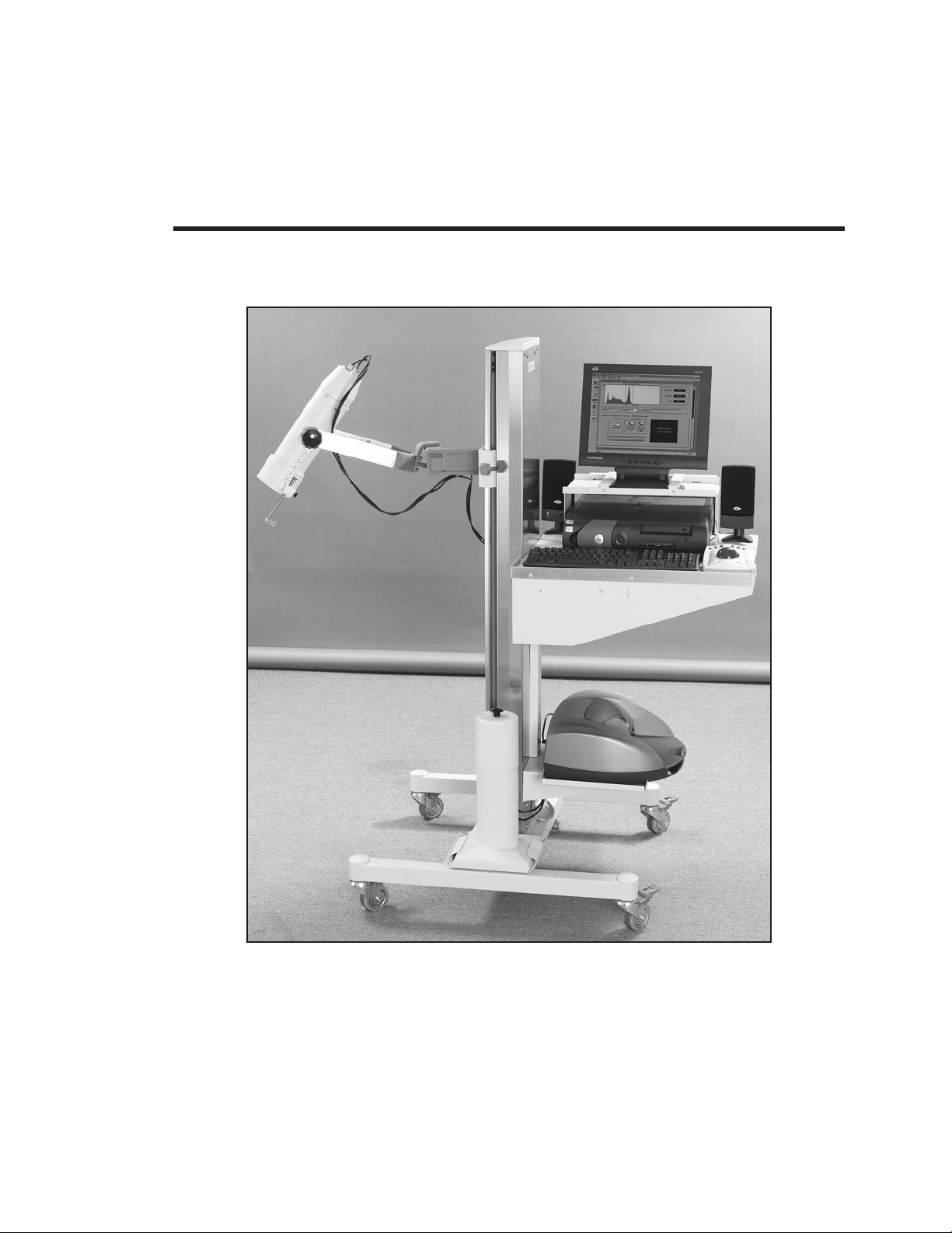
ATOMLAB 950 (PC)
MEDICAL SPECTROMETER

SERVICE/OPERATION MANUAL

187-130
187-135
187-140
187-145

FN: 05-211 6/05

BIODEX

20 Ramsay Road, Shirley, New York, 11967-4704, Tel: [phone] (In NY and Int’l, call 631-924-9000), Fax: [phone], Email: [email protected], www.biodex.com

Biodex Medical Systems, Inc.

ATOMLAB 950 (PC)

0413

This manual covers installation and operation procedures
for the following Atomlab 950 products:

#187-130 115 VAC, Table Top, Thyroid Uptake System, Atomlab 950
#187-135 230 VAC, Table Top, Thyroid Uptake System, Atomlab 950
#187-140 115 VAC, Mobile, Thyroid Uptake System, Atomlab 950
#187-145 230 VAC, Mobile, Thyroid Uptake System, Atomlab 950

NOTE: All or some of the following symbols, cautions, warnings and notes may apply to your Atomlab 950

and correspond to this operation manual:

Symbol Meaning

Attention, consult accompanying documents.

Symbol signification: Attention, se référer à la notice.

Warning: Injuries to health may result from incorrect or excessive training.

Attention, incorrect ou extrême entrainement peut aboutir des lesíons au santé.

NOTE: Circuit diagrams for this product are available upon request.

IMPORTANT NOTES

• Before you use this device, be certain to read the entire manual. Failure to read this manual may
result in user error or inaccurate data.

• All activities and count values on the sample reports in this manual are for illustration purposes
only. They do not represent actual study values.

Authorized European Community Representative: Prothia, Paris, France

WARRANTY

ATOMLAB Thyroid Uptake Systems carry the industry’s best warranty.

Biodex Medical Systems backs Atomlab Thyroid Uptake Systems with a truly comprehensive full
two-year warranty. It covers both parts and labor, and includes all unit elements. Biodex’s two-year
warranty is a sure sign of product quality and dependability.

With this two-year warranty, quality assurance, guaranteed delivery from stock, and responsive
customer service, Biodex Medical Systems gives the nuclear medicine field the right answer… Atomlab
Thyroid Uptake Systems.

TABLE OF CONTENTS

1. Introduction ........................................................................................................................1-1

2. Setup Instructions..............................................................................................................2-1

• Assembly Procedure ..........................................................................................................2-1

• System Shut-Down............................................................................................................2-7

• General Cleaning Instructions ..........................................................................................2-7

• Power-Up and Self-Test ....................................................................................................2-7

• Computer Preliminaries ....................................................................................................2-8

• System-Wide Icons ............................................................................................................2-8

• System Software Setup ....................................................................................................2-13

• Edit Physicians and Technologist Database......................................................................2-15

• Database Manager ..........................................................................................................2-17

3. Administration ....................................................................................................................3-1

• Daily Calibration ..............................................................................................................3-1

• High Voltage Adjustment ................................................................................................3-5

• Chi-Square ........................................................................................................................3-8

• Administration Report ....................................................................................................3-11

• Isotope Editing ................................................................................................................3-11

• Isotope Efficiencies ..........................................................................................................3-18

• Detector Efficiency ..........................................................................................................3-20

• Spectrum Analysis ..........................................................................................................3-22

• How is ROI Determined? ................................................................................................3-24

4. Thyroid Uptake ..................................................................................................................4-1

• Defining a Facility Standard Uptake Procedure..................................................................4-1

• Patient Definition Screen ..................................................................................................4-4

• Determining Automatic Count Time ................................................................................4-5

• Performing a Thyroid Uptake ............................................................................................4-7

• Printing a Thyroid Uptake Report ..................................................................................4-12

• Printing a Time Activity Uptake Report..........................................................................4-12

5. Manual Mode ....................................................................................................................5-1

• To Count in Manual Mode ................................................................................................5-1

• To Print in Manual Mode ..................................................................................................5-1

• Spectrum Analysis ............................................................................................................5-1

6. Wipe Test..............................................................................................................................6-1

• Define Wipe Areas ............................................................................................................6-1

• Select Wipe........................................................................................................................6-5

• Wipe Preferences ..............................................................................................................6-7

• Performing a Wipe Test ....................................................................................................6-9

• Spectrum Analysis ............................................................................................................6-9

7. Bioassay ..............................................................................................................................7-1

• To Perform a Bioassay ........................................................................................................7-2

8. Schilling Tests ......................................................................................................................8-1

• To Determine a Facility Standard Schilling Test ................................................................8-1

• To Perform a Schillings Test (Bracco, Mallinckrodt or Simple Mallinckrodt) ......................8-1

• Schilling Dicopac ..............................................................................................................8-5

• Spectrum Analysis ............................................................................................................8-8

TABLE OF CONTENTS 4

1. INTRODUCTION

9. Hematology........................................................................................................................9-1

• The Hematology Patient Page ..........................................................................................9-1

• IHSA I-125 ......................................................................................................................9-1

• Cr-51 Blood Volume..........................................................................................................9-3

• Cr-51 Red Cell Survival ....................................................................................................9-9

• GFR ................................................................................................................................9-11

• Effective Renal Plasma Flow ............................................................................................9-17

Appendix A: Isotope Efficiency Calculation ........................................................................A-1

Appendix B: Specifications ................................................................................................B-1

Appendix C: Electromagnetic Compatibility ....................................................................C-1

Schematics..........................................................................................................................S-1

5 TABLE OF CONTENTS

1. INTRODUCTION

The Atomlab 950 PC is a complete thyroid uptake and analysis system specifically designed for nuclear
medicine. Capable of performing a full range of studies this system provides fast, accurate results for
Uptake Studies, Bioassay, Wipe Testing, Schilling Tests programmed for the Mallinckrodt, Bracco, or
Nycomed Dicopac® Schilling kits and Hematology testing.

The heart of the Atomlab 950 is a microprocessor-controlled 1024 channel Multi-Channel Analyzer,
coupled to a 2" x 2" NaI(Tl) detector with a personal computer interface. The system offers simple,
straight-forward operation using 23 pre-programmed isotopes, 50 user-defined radionuclides, and menu­driven prompts to guide the user step by step through each procedure. The pre-programmed
radionuclides include I-123, I-125, I-131, Co-57, Cr-51, Tc-99m and Cs-137. The user-defined radionuclides
also allow for isotope identification while the printer provides hard copy printouts for patient and
department record keeping.

The Atomlab 950 has a memory allowing storage of 5,000 patients with multiple uptakes on each.
Additional features include an automatic self-diagnostic program, automatic calibration mode, choice of
automatic or manual counting time for uptake studies, and automatic isotope decay correction of uptake
measurements. These features help make this the most simple and accurate thyroid uptake system
available today.

INTRODUCTION 1-1

2. SETUP INSTRUCTIONS

Assembly Procedure

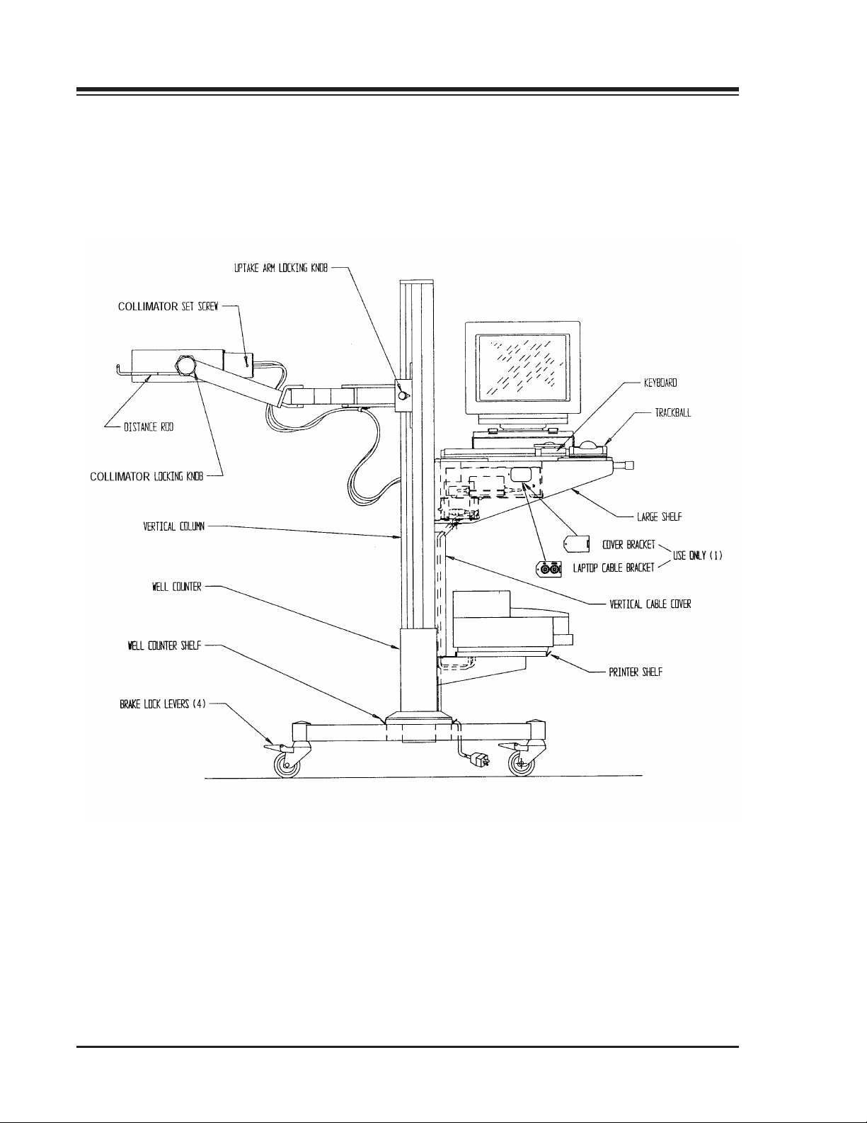
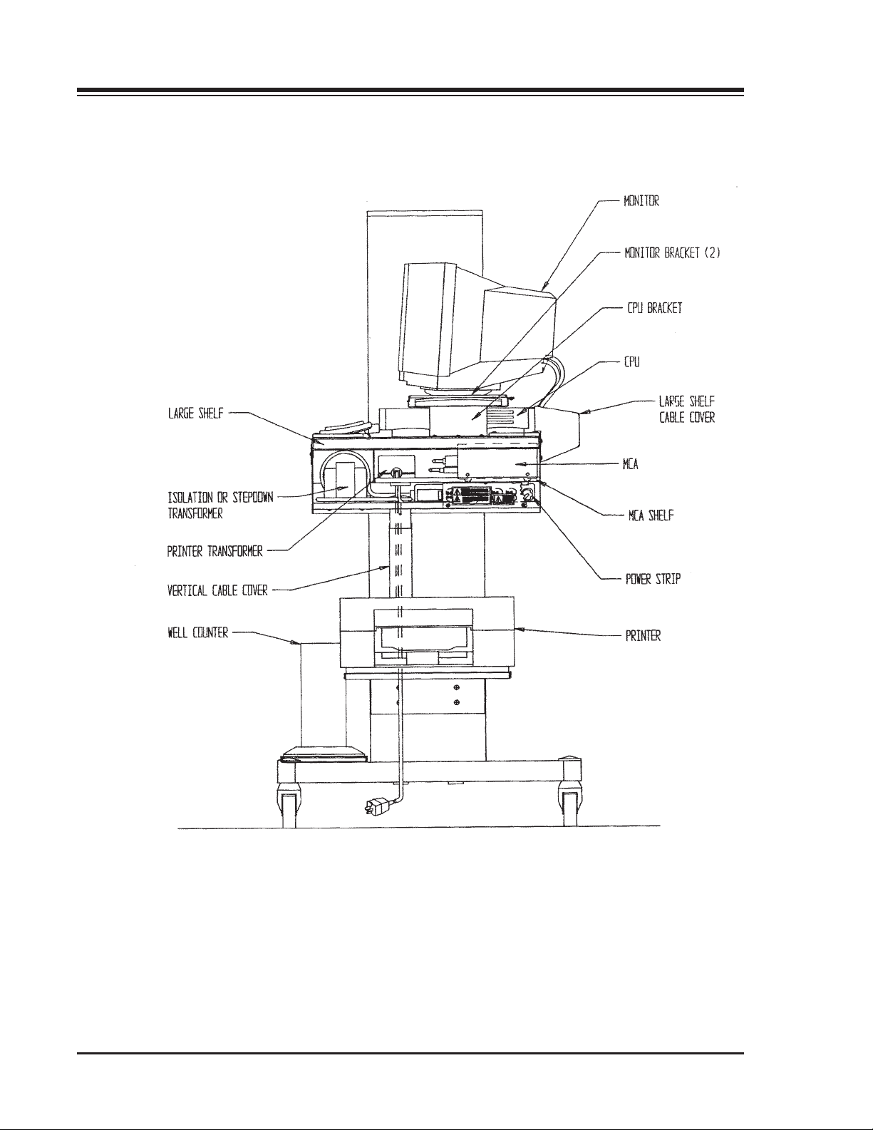
(See Figures 2-1 and 2-2.)

Tools Required:

Knife
Wire cutter
Phillips screwdriver
Medium straight screwdriver
Small straight screwdriver
1/32" Allen key (included)
Adjustable wrench

1. Remove the uptake stand from its shipping box and place in an area suitable for assembly and setup.

2. Determine how the unit will be positioned in the department where it is to be used. The computer,
keyboard, CPU and monitor will need to be installed correspondingly, facing to either the left or
right of the large shelf push bar on the stand. The normal configuration is the keyboard to the left of
the push bar.

3. If you desire to change the orientation, use a Phillips screwdriver to remove the six screws that hold
the CPU bracket to the top of the large shelf. Remove the bracket and place it aside, retaining the
screws.

4. With a Phillips screwdriver, remove the four screws that hold the large shelf cable cover to the side
of the large shelf. Remove the cable cover and place it aside, retaining the screws.

NOTE: The cables may be already installed into the stand.

5. With a Phillips screwdriver, remove the three screws that hold the vertical cable cover to the vertical
column. Remove the vertical cable cover and place it aside, retaining the screws.

6. If you will be using the optional well counter with your system, ensure that the well support shelf is
on the appropriate side of the stand. It should be positioned on the same side that the keyboard will
be positioned. To move the well counter shelf to the opposite side, use a medium slotted screwdriver
to remove the four screws that hold the well support shelf in place, remove the shelf and replace the
screws. Now remove the four screws on the other side of the vertical column and use these to secure
the well.

7. The large shelf side cable hole cover should be positioned on the same side as the keyboard. If it is
not, use a Phillips screwdriver to remove the screw that holds the cover to the large shelf. Remove
the plastic gasket from the opposite side cable hole and position it on the hole from which the cover
was just removed. Now take the large shelf side cable hole cover and install it on the opposite side
(the side from which the plastic gasket was just removed).

8. Using a small slotted screwdriver, remove the two screws that hold either of the well support
brackets to the well support shelf. Remove this bracket, then loosen the screws on the remaining
bracket so that the bracket has a small degree of play.

9. Remove the well counter and two cables (located in the base) from their shipping carton. Slide the
well counter onto the well shelf so that the cable connectors are facing in the same direction as the
large shelf push bar. Ensure that the well support bracket which is still attached to the well support
shelf is positioned over the edge of the well counter base. With a straight screwdriver, tighten the
two screws to secure the well support bracket over the well counter base.

10. Using a small straight screwdriver, replace the well support bracket removed in step #8. Ensure that
the bracket is positioned over the edge of the well counter base before tightening the two screws that
hold it in position. Ensure that both well support brackets are firmly in place.

2-1 SETUP INSTRUCTIONS

1. INTRODUCTION

Figure 2-1. The MCA Uptake Stand.

SETUP INSTRUCTIONS 2-2

CONTENTS

11. Connect the two well counter cables to the well counter fittings. The larger connector (MHV) should
be connected to the high voltage fitting on the well. The smaller connector (BNC) connects to the
well signal fitting. Allow the ends of both cables to lie off to the side.

12. On the underside of the large shelf, directly below the MCA shelf, is a power strip. If your unit has a
cover over the plug sockets (some units do not), use a Phillips screwdriver to remove the three
screws that hold the cover in place. Place the cover aside, retaining the screws.

13. Open the printer box and remove the small box containing the printer power pack. Place the power
pack onto the MCA shelf directly above the power strip, or onto the shelf with the powerstrip.

14. Route the 3-prong power plug from the printer power pack down through one of the MCA shelf
cable holes and plug it into the power strip. Now take the long power pack cable with the
rectangular end, route it along the back of the MCA shelf and down through the left side MCA shelf
cable hole. Continue to route this cable down through the large shelf vertical cover cable hole, down
through the printer shelf vertical cover cable hole and, finally, back up through the printer shelf
cable hole. Allow eight to ten inches of the cable to protrude through the printer shelf cable hole.

15. Take the two well counter cables and route them under the printer shelf, up through the printer shelf
vertical cover cable hole, through the large shelf vertical cover cable hole and, finally, through the
MCA shelf cable hole. Pull the cables snug and allow them to hang out from the front of the MCA
shelf.

16. Locate the printer cable. Run the strip end of this cable through the large shelf side cable hole, down
through the large shelf vertical cover cable hole, down through the printer shelf vertical cover cable
hole, and finally, back up through the printer shelf cable hole. Allow eight to ten inches of the cable
to protrude through the printer shelf cable hole.

17. Reinstall the vertical cable cover using a Phillips screwdriver and the three screws removed in step
#5. Ensure that cables are tucked neatly inside the cover.

18. Removethe printer fromthe printer box and placeit on the printer shelfso that the front faces thesame direction
as the large shelf push bar. Connect the printer power pack cable and the printer signal cable to the appropriate
ports on thebackof theprinter.Tomakethese connections, turnthe printer to expose the connection ports.

19. Open the cover on the printer and remove the tape that holds the print carriage from moving. Open
up the print ink cartridge packs and slide them into the print carriage on the printer. The cartridge
should slide in, then snap back into position. Place a stack of paper in the paper tray.

20. Loosen the collimator locking knob and rotate the collimator into a vertical position with the
distance rod facing down. Tighten the locking knob.

21. If you have not already done so, use an adjustable wrench to remove the RED shipping bolts located
near the vertical lock knob. (This bolt keeps the arm from moving during shipment.)

22. If necessary, adjust the uptake arm height. To do this, loosen the vertical column locking knob and
slide the counter-balanced arm to the desired position. Tighten the locking knob to secure the uptake
arm at the desired height.

23. Near the top of the collimator, locate the set screw. Use the supplied 1/32" Allen wrench to loosen
the screw in a counterclockwise direction until it retreats enough to allow passage of the tube
assembly into the collimator.

2-3 SETUP INSTRUCTIONS

1. INTRODUCTION

Figure 2-2. The MCA Uptake Stand. (side view).

SETUP INSTRUCTIONS 2-4

CONTENTS

24. Remove the tube assembly and base from its packaging. Notice that a grounding strap is wrapped
around the base and tube assembly. This is necessary to properly ground the detector shroud to the
base and stabilize the count rate. Remove the red protective cap from the detector and carefully
insert the detector and base assembly into the cone shaped collar. Slide the detector downward until
the entire assembly is inserted. At this point, the detector cables should be flush with the top of the
collimator. Tighten the set screw to secure the detector in place.

NOTE: Do not force the assembly into position as it is possible to dent the shroud and damage the detector. If
the assembly will not slide easily into place, check to make sure the set screw has been sufficiently loosened.

25. Route the detector cables between the collimator and the uptake arm collimator yoke. Loosen the
collimator tilt locking knob and tilt the collimator so that the detector cables are in the furthest
position possible from the uptake stand vertical column (be sure to extend the collimator arm fully).

26. Insert the larger (MHV) detector cable connector through the large shelf back cable hole (alongside
the vertical column). You can now push the smaller (BNC) detector cable connector through the
same hole. Pull both cables out through the front of the MCA shelf and allow them to hang free.

27. Using a straight screwdriver, remove the wire wrap from the underside of the collimator arm. Place
the wire wrap around both detector cables and reinstall to the collimator arm. Before securing the
wire wrap screw, set the cables so that there is a little slack leading to the detector.

28. Remove the CPU from its packaging and place it on top of the large shelf. Make sure it faces the
front of the stand where the operator will be working.

29. Slide the CPU toward the back of the large shelf. Place the keyboard and trackball mouse on the
shelf in front of the CPU. The keyboard should be to the left of the trackball.

30. Run the free end of the keyboard cable along the side of the CPU and plug it into the keyboard port
at the back of the CPU.

31. To install the trackball, attach one end of the trackball cable to rear of the trackball. Run the opposite
end of the cable inside the CPU hold-down and plug it into mouse port on the rear of the CPU.

32. Take the CPU bracket that was removed in step #3 and position it over the CPU. The bracket lip
with the slotted holes should face towards the front of the CPU. With a Phillips screwdriver, reinstall
the six screws that secure the bracket to the large shelf. The keyboard cable should be on the inside
of the bracket so it is under the CPU.

33. Remove the monitor from its packaging and place it on top of the CPU bracket so that the monitor’s
swivel base is centered on the bracket.

34. Swivel the monitor 45 degrees and hook the front of the monitor bracket to the CPU bracket. With a
Phillips screwdriver and single screw, secure the back end of the monitor bracket to the CPU
bracket. Repeat this procedure to secure the opposite monitor bracket.

35. Run the monitor signal cable (one end fixed to the back of the monitor) into the monitor port at the
back of the CPU (an adapter may be required).

36. Plug the monitor power pack into the powerstrip. Run the other end of the power pack cable up the
right side hole and out the side of the stand. Now plug it into the monitor.

37. Take the female end of another power cord and plug it into the back of the CPU. Route the male end
of the cord through the large shelf side cable hole and down through the MCA shelf cable hole. Plug
the power cord into the power strip.

2-5 SETUP INSTRUCTIONS

CONTENTS

38. Locate the printer cable that now protrudes from the large shelf side cable hole and plug it into the
CPU printer port.

39. Unpack the speakers and place them on the large shelf. Connect the double cable from the rear of the
CPU speaker connector (the connector next to the 9-pin DIN connector.)

40. Connect the phone jack.

41. Connect the free end of the double cable to the input connector on the speaker.

42. Run the single cable from the right speaker to the left speaker. Plug the speaker power pack into the
power strip. Now run the cable up through the hole with all the other power cords. Pull the cable
out the vertical hole and connect it to the speaker power input connector.

43. Unpack the MCA box and power cord. Route the male end of the power cord over the MCA shelf
and down through the MCA shelf cable hole. Plug the cord into the power strip. Allow the female
end of the power cord to protrude from the MCA shelf.

44. The MCA signal cable has a 9-pin female connector on one end and a 9-pin connector on the other.
Connect one connector to the COM 2 port on the back of the CPU. Route the 9-pin connector
through the large shelf side hole and onto the MCA shelf. Pull the cable and allow it to hang over the
front of the MCA shelf.

45. While holding the MCA box in front of, or just below, the MCA shelf, use a straight screwdriver to
connect the 9-pin connector to the open port on the back of the MCA.

46. Connect the two probe cables, which now extrude from the front of the MCA shelf, to the
appropriate fittings on the back of the MCA. The larger connector (MHV) is for high voltage, the
smaller (BNC) connector is for signal.

47. If you have a well counter, connect the larger (MHV) well cable connector to the well high voltage
fitting and the smaller (BNC) connector to the well signal port on the back of the MCA.

48. Plug the female end of the power cord into the back of the MCA. As much as possible, gather and
neatly bundle all the cables so that they lie outside the large shelf where they can later be covered by
the large shelf cable cover.

49. Place the MCA box on the MCA shelf so that the front of the MCA faces the side of the shelf with the
power ON/OFF switch accessible to your left so that it can be easily turned ON and OFF if required.

50. Make sure that there is paper in the printer tray. If not, add a stack of paper.

51. Plug the main power cable for the uptake stand into a hospital grade wall outlet. Turn the power
strip ON and make sure that all the units power up as indicated by their LEDs. If any component is
not ON at this point, try flipping the Power ON switch for that component and check that the plugs
are inserted properly into both the power strip and into the component.

52. If all components are ON, use a Phillips screwdriver to replace the large shelf cable cover removed
in step #4, making sure that the cables which protrude from the large shelf side cable hole are neatly
gathered and covered by the cover.

53. With a Phillips screwdriver, reinstall the power strip cover removed in step #12.

SETUP INSTRUCTIONS 2-6

1. INTRODUCTION

SYSTEM SHUT-DOWN

The Atomlab 950 system is now fully set up and ready for operation. Before it can be moved, however, it
must be shut down using the following procedure.

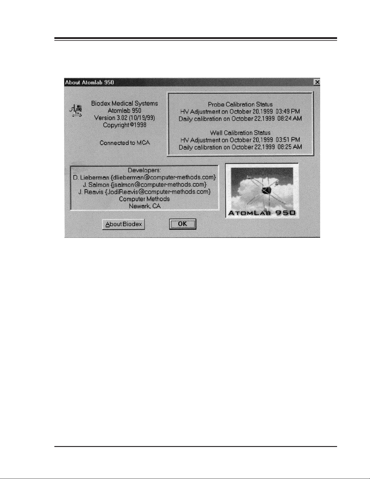
1. At the Windows Desktop screen, which should now be displayed, move the trackball pointer over
the “Atomlab950” icon and double-click the mouse. The About Atomlab950 screen should now be
displayed. A calibration status box is located on the right side of this screen.

2. Look below the version number of the Atomlab software (under the Biodex Address on the left side
of the screen) and check the detector status. If the cables are connected properly at this point, there
will be a message reading "Connected To MCA."

NOTE: If the message reads "Device Not Found," reconnect the cables leading to the MCA and check all other
connections. If the system will not connect to the MCA, click on <No> and then click on <Yes> to advance to
Simulation mode. You can then exit Simulation mode by clicking on <File> at the top of the screen, selecting
<System Setup>, and then clicking on <Simulation Mode> to remove the check mark. See "System Software
Set Up."

3. If the detector status is okay, click on <OK> to advance to the MCA Operation screen.

4. Move the pointer over the <X> at the top right corner of the screen and click the left trackball button
to exit. The Windows Desktop should now be displayed.

5. Select <Start>. Now click on <Shut Down> and then <OK>. The system will now take several
seconds to shut down the computer. When finished, a message will appear on the screen noting that
it is safe to turn the system OFF. Turn the power strip off at this time. You can now unplug the
system and move it to the location where it will be used.

NOTE: The push handle can be used as a wire wrap to hold the uptake stand power cord during transport.

GENERAL CLEANING INSTRUCTIONS

As required, wipe down the exterior of the unit using a soft rag slightly dampened with alcohol.

POWER-UP AND SELF-TEST

(See Figures 2-3 and 2-4.)

At this point, your Atomlab 950 Medical Spectrometer should be fully ready for operation. It is
recommended that the system be turned ON at least one hour before use or, if possible, left on at all
times. This will provide optimum performance and will not effect the longevity of any part or component
except the monitor, which should be turned OFF if the Atomlab 950 will not be used for a prolonged
period of time.

To Power-Up And Run The Self-Test

Turn on all components, including the printer. The system may immediately advance to the Atomlab 950
program. If not, double-click on the <Atomlab950> icon from the system desktop. Once the Atomlab 950
program is activated, the system immediately performs a self-test. The About Atomlab 950 screen is then
displayed.

NOTE: If the system is in Simulation Mode, see System Setup later in this manual to return to normal operating
mode.

2-7 SETUP INSTRUCTIONS

CONTENTS

The Self-Test includes:

• MCA firmware and hardware checks

• DAC value verification

• Display of software/firmware revisions

NOTE: To view a video clip about the Biodex Company, you can at this point click on <About Biodex>.

Once the self-test is complete, the system highlights <OK>. Click on <OK> to automatically advance to
the MCA Operation screen. The system is now ready for use.

COMPUTER PRELIMINARIES

Windows Format

The Atomlab 950 PC is a personal computer (PC) based system. All menus and screens function in
standard windows fashion. Each screen prompts the user, either through screen prompts or icons, as to
all available options. As you begin to explore the Atomlab 950 menus, you’ll quickly learn that some
options are available from every screen, others are offered only on selected screens and some are specific
only to the operation being performed.

Using the Mouse

While numeric “data” is entered into the system by simply typing on the keyboard, options, menus and
pages are selected via the trackball mouse. The trackball is simple to use, it responds instantly to all
movement by positioning the screen pointer appropriately. To select any option on the screen, simply use
the trackball to locate the cursor over the desired icon and click the left trackball button. An hour glass
icon appears over the selected option icon, indicating that the system is advancing to the selected option.
After a second or two, the new menu, screen or page appears.

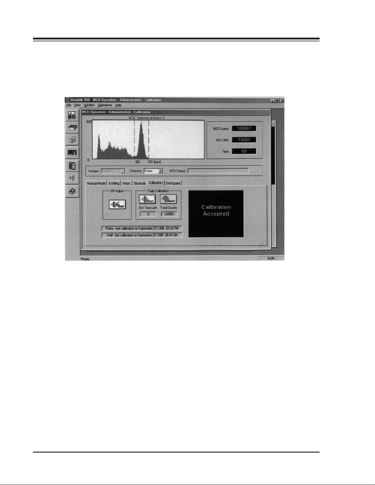
To see how the mouse works, select the <Calibration Tab> in the middle of the Operation screen. The
Daily Calibration page should appear if it is not already displayed. Now, select the <Manual Tab> to
access the Manual Counting screen.

Select the <Calibration Tab> once again to return to the daily calibration page.

SYSTEM-WIDE ICONS

(See Figure 2-5.)

The Primary Tool Bar

The tool bar along the left side of the screen allows users to quickly and easily access the primary modes
of operation and screens as follows. Each option is described below in descending order from the top of
the tool bar.

• Patient Definition: This screen allows patients to be added, removed, edited or saved.

• MCA Operation: Click on this icon to return to the MCA operation screen or Main Menu of the
Atomlab program.

• Report Generation: Click on this icon to access the various different printout options associated
with all the modes on the system.

SETUP INSTRUCTIONS 2-8

1. INTRODUCTION

Figure 2-3. Click <OK> on the About Atomlab 950 Screen to Begin the Self-Test.

2-9 SETUP INSTRUCTIONS

1. INTRODUCTION

Figure 2-4. The Atomlab 950 PC Operation Screen is displayed at completion of the self-test. The system is now ready

for use.

SETUP INSTRUCTIONS 2-10

1. INTRODUCTION

• Spectrum Analysis: After most counting functions click on this icon to view a full page display
showing the Spectrum Analysis. You can then adjust ROIs, add ROIs and move a cursor to see
the energy and counts associated with different energies.

• Procedure Window. Click on this icon to define the different procedures that you want to use.
An example would be to have different methods of the thyroid uptake stored in memory to be
used for different types of uptake studies.

• Isotope Editing: At this page you can bring up the list of factory set isotopes or enter any new
isotopes that you desire. This mode will also allow the efficiency setting for the detectors for
specific isotopes used for Bioassay and Wipe.

• Help: This screen will give certain information about using the system.

Screen Tool Bar

The screen tool bar, located at the top of most major screens, features several buttons that standard
conventions in the system and appear on a variety of pages.

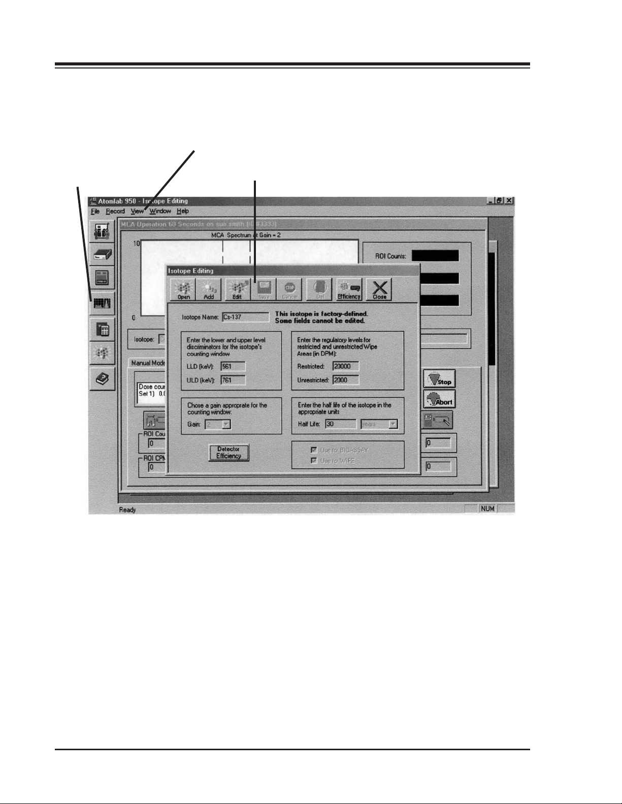
Click on <Isotope Editing> in the primary tool bar on the left side of the screen to bring up the Isotope
Editing page. On this page, you can view the screen tool bar and follow along with the descriptions
below.

• Open: Click on this button to access a list of the items associated with the current function. For
example, if you are dealing with isotopes, it brings up the isotope list.

• Add: This button allows you to add an item to the current operation. For example, on the
isotope page, you can add an isotope. On the patient page, you can add patients.

• Edit: This button allows you to go in and edit the item that you are displaying.

• Save: Use this option to save any changes or new information that you have entered on the
current page.

• Stop/Cancel button will cancel whatever work you were just doing without saving any
changes.

• Delete: Use this option to delete information that you have entered. For example, if you entered
a patient and are now finished with that patient, you could delete the patient from the system
memory.

• Efficiency: Use this button to enter efficiencies for each isotope associated with wipe and
bioassay.

• Close: Select this button to close any current window.

Click on <Close> to return now to the Operation screen.

The Menu Bar

The Menu Bar very top of the desktop screen offers standard Windows functions including File, Record,
View, Window and Help. The system setup and print-setup options are both accessed by selecting <File>
from this menu bar.

• File: Under the File screen, the printer set up button allows you to set up the printer that you
are using. The Atomlab 950 uses either DeskJet 694C, 845 or 810C software. The version used is
dependent on the Hewlett Packard printer. We recommend using the 694C printer driver. If a
different printer is being used, follow the instructions for setting up under Windows. The
Database Manager option allows the user to copy or move data. The System Setup button
allows the user to set site information.

2-11 SETUP INSTRUCTIONS

1. INTRODUCTION

Menu Bar

Primary Tool Bar

Screen Tool Bar

Figure 2-5 The Isotope Editing Screen.

SETUP INSTRUCTIONS 2-12

X

• View: The View option allows you to view in different modes.

• Window: Allows cascading, horizontal or vertical placement of windows.

• Operations: Allows access to different operating modes.

• Help: Provides help on specific system topics.

The computer operation is a standard Windows format and the Windows format should be used for
setting date and time.

SYSTEM SOFTWARE SET UP

(See Figure 2-6.)

The System Setup option allows the user to enter site information including the facility name, address
and phone number. It also allows editing of the physician and technologist database, and allows the
system to be set for Simulation or Active mode.

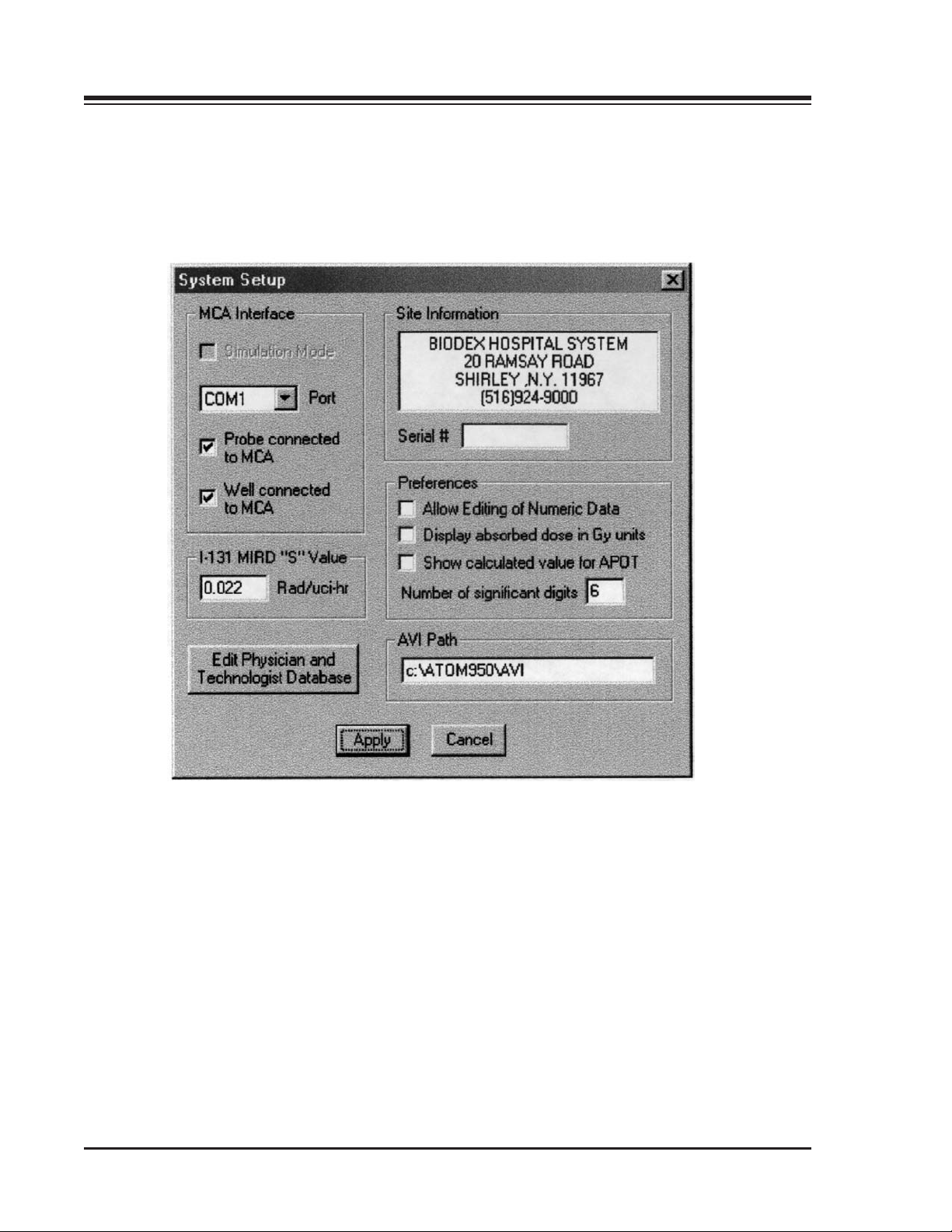
To access system setup, click on <File> in the menu bar, then click on <System Setup>. At this screen, a
check in the box preceding any option means that the option is active. To activate or deactivate any
option, click the mouse on the appropriate option box. Setup options are described below.

MCA Interface

• Simulation Mode: In Simulation mode, the Atomlab 950 will provide mock measuring without

the need for actual activity. This mode allows the user to explore the various screens and
modes of the system.

NOTE: EXITING SIMULATION MODE
When the Atomlab 950 System is turned ON and the MCA box is OFF, the computer prompts you to select
Simulation mode if desired. If you select Simulation mode, the system returns to the desktop. You can then click on
<Start>, followed by <Programs>, <Biodex Medical Systems>, and <Atomlab 950 Simulation> to enter Simulation
mode.

To exit Simulation mode, click on the <X> in the upper right corner of the screen to return to the desktop. You can
then turn the MCA box ON and double-click on the Atomlab 950 desktop icon to access the Atomlab 950 Active mode.

• Port: The port listed is for the MCA box connection. The standard configuration has the MCA
box connected to COM 2. The small arrow in the box allows the system to function as a
standard pull-down menu.

• Probe or Well: If your system has only one detector, there should be a check mark next to the
detector only. This will make the detector your only choice on the menu. If you add a detector
at a later time, you will need to access system setup and put a check next to the appropriate
detector to make it available for use.

I-131 MIRD "S" Value

This is preset for 0.022 rads per microcurie hours. Enter any desired change and click on <Apply> The
changes will cause you to restart the system before they can be applied. If you don't want to make any
changes, click on the <Cancel>.

Thyroid Uptake Report

Use the arrow in the box to choose between Efficiency Half-Life and Biological Half-Life.

Site Information

Enter here your facility name and address. The facility name entered here will appear on all printed
reports.

2-13 SETUP INSTRUCTIONS

1. INTRODUCTION

Figure 2-6. The System Setup Screen.

SETUP INSTRUCTIONS 2-14

X

Preferences

Check any option here to activate.

• Numerical Data: If checked, allows the operator to change the time and data of administration
as well as change the count before it is saved in a mode. For example: If you count background
and uptake before you save, you can go in and modify this value.

• Display Absorb Dose In GY Units: Activate this option to display the dose in GY units in the
special decay function program.

• Show Calculated Value For APOT (Analyzed Pulses Over Total Pulses.) This is a diagnostic tool
that will show as you count. Normal operation for users would have this inactive.

• Number Of Significant Digits: The system is preset for 4. Enter the desired number to change.

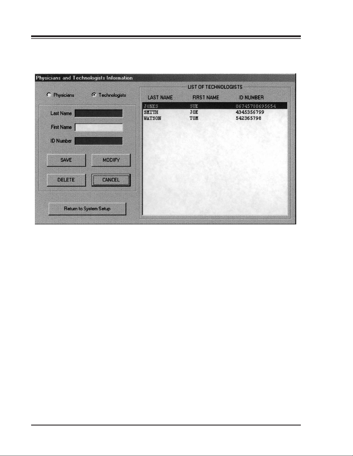
Edit Physician and Technologist Database

(See Figure 2-7.)

To add a new physician or technologist to the database:

1. Click <Edit Physician and Technologist> to access the Edit Physician and Technologist screen.

2. Click <Physician> or <Technologist> to highlight the desired database. The physician or
technologist list will be displayed on the right of the screen.

3. Key in the physician or technologist last name, first name and ID number. Use the mouse or <Tab>
keys to move from field to field.

4. Click <Save> to save the new entry to the database.

5. Click <Return to System Setup> to return to the System Setup screen.

To edit a physician or technologist:

1. Click <Edit Physician and Technologist> to access the Edit Physician and Technologist screen.

2. Click <Physician> or <Technologist> to highlight the desired database. The physician or
technologist list will be displayed on the right of the screen.

3. Click on the physician or technologist to edit, then click <Modify>. The selected entry is now
displayed in the edit fields on the left side of the screen.

4. Edit the appropriate fields. Use the mouse or <Tab> keys to move from field to field.

5. Click <Save> to save the new entry to the database.

6. Click <Return to System Setup> to return to the System Setup screen.

To delete a physician or technologist:

1. Click <Edit Physician and Technologist> to access the Edit Physician and Technologist screen.

2. Click <Physician> or <Technologist> to highlight the desired database. The physician or
technologist list will be displayed on the right of the screen.

3. Click on the physician or technologist to delete. The selected entry is now highlighted. The system
request confirmation that the entry is to be deleted. Click <Yes> to delete.

4. Click <Return to System Setup> to return to the System Setup screen.

2-15 SETUP INSTRUCTIONS

1. INTRODUCTION

Figure 2-7. The Edit Physicians and Technologists Information Screen.

SETUP INSTRUCTIONS 2-16

AVI Path

This shows the current directory path of the computer files in use. Leave this setting at the default value.

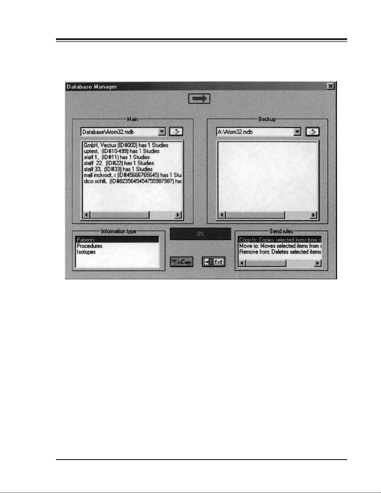
DATABASE MANAGER

(Refer to Figure 2-8.)

The Database Manager portion of the program allows patient information, procedures specifications or
isotope information to be saved to a floppy diskette or other information storage format.

To Save Patient Specific Data:

1. Click on <Patient Definition> to open the patient definition window.

2. Insert a blank floppy diskette into the floppy drive.

3. Click on <File> in the menu bar, then click <Database Manager> on the drop-down list. The
Database Manager screen is now displayed. The left side of the screen displays the current
information while the right side shows where the data will be stored or transferred.

4. To save a specific patient's data, click on that patient in the left hand column. The arrow at the top of
the page will then point to the right, which is labeled “Backup.”

NOTE: Drive A: should be shown as the back-up destination. If drive A: is not displayed as the back-up
destination, use the Back-up drop-down menu to select Drive A:. If Drive A: is not displayed as an option on
the Back-up drop- down menu, click on the “...” box below “Backup” at the upper right of the screen. Choose 3­1/2" Floppy (A) from the drop-down menu to select drive A, then click on <Open>. The system should return
to the Back-up screen with drive A: now selected.

6. Click on the <Copy> button in the bottom center of the screen to duplicate the source file onto the
floppy.

NOTE: To copy all of the patients in the database, you can highlight all the patients by clicking on the first one
and then sliding the pointer down to cover all the patients. Click on <Copy> and all patient data for all
patients will be transferred to the floppy.

To Transfer or Restore Data From A Floppy To The Hard Drive:

1. Click on <Patient Definition> to open the patient definition window.

2. Click on <File> in the menu bar, then click <Database Manager> on the drop-down list. The
Database Manager screen is now displayed. The left side of the screen displays the current
information while the right side shows where the data will be stored or transferred.

3. Highlight the right hand column upper window and type in A:\. Highlight the specific patient or
patient data that you wish to transfer to the hard drive. When you click on the right hand column,
the arrow at the right will show the direction the data will move. When this is correct, press the
<Copy> at the bottom of the screen.

NOTE: The <Move> function works like the copy function. It removes it from the original database and puts
it into the backup database.

2-17 SETUP INSTRUCTIONS

To Remove Data:

1. To remove data in the bottom hand box, click on <Remove>.

2. Highlight the data or item in the right hand box that you wish to remove.

3. Click on <Remove> and a pop-up window will ask if you really want to remove this data. If you do,
click <Yes> and the system will proceed to remove the information. When you are done, click on the
<Exit> button in the center and this will take you back to the regular Atomlab program.

NOTE: If there is already data in a patient file, you must delete that patient in the backup before you can
transfer from the original data.

NOTE: To back-up “procedures” you must save the Isotope information to the backup before transferring the
procedures.

SETUP INSTRUCTIONS 2-18

1. INTRODUCTION

Figure 2-8. The Database Manager Screen.

2-19 SETUP INSTRUCTIONS

3. ADMINISTRATION

Before using the Atomlab 950 PC for counting purposes, it is important that you take a few minutes and
prepare the system for operation. The following functions are set from the Operation screen and control
the system throughout the different program modes.

NOTE: Before you begin with this chapter, be sure to enter your facility name and address in the Site Information
area, as explained in the section on System Setup. This will allow the system to print the facility name on all
printouts

• Daily Calibration

• Chi-Square Test

• High Voltage Adjustment

• Isotope Editing

• Isotope Efficiencies

• Detector Efficiency

• Analysis (also available for each operation)

• MCA Operation

Daily Calibration

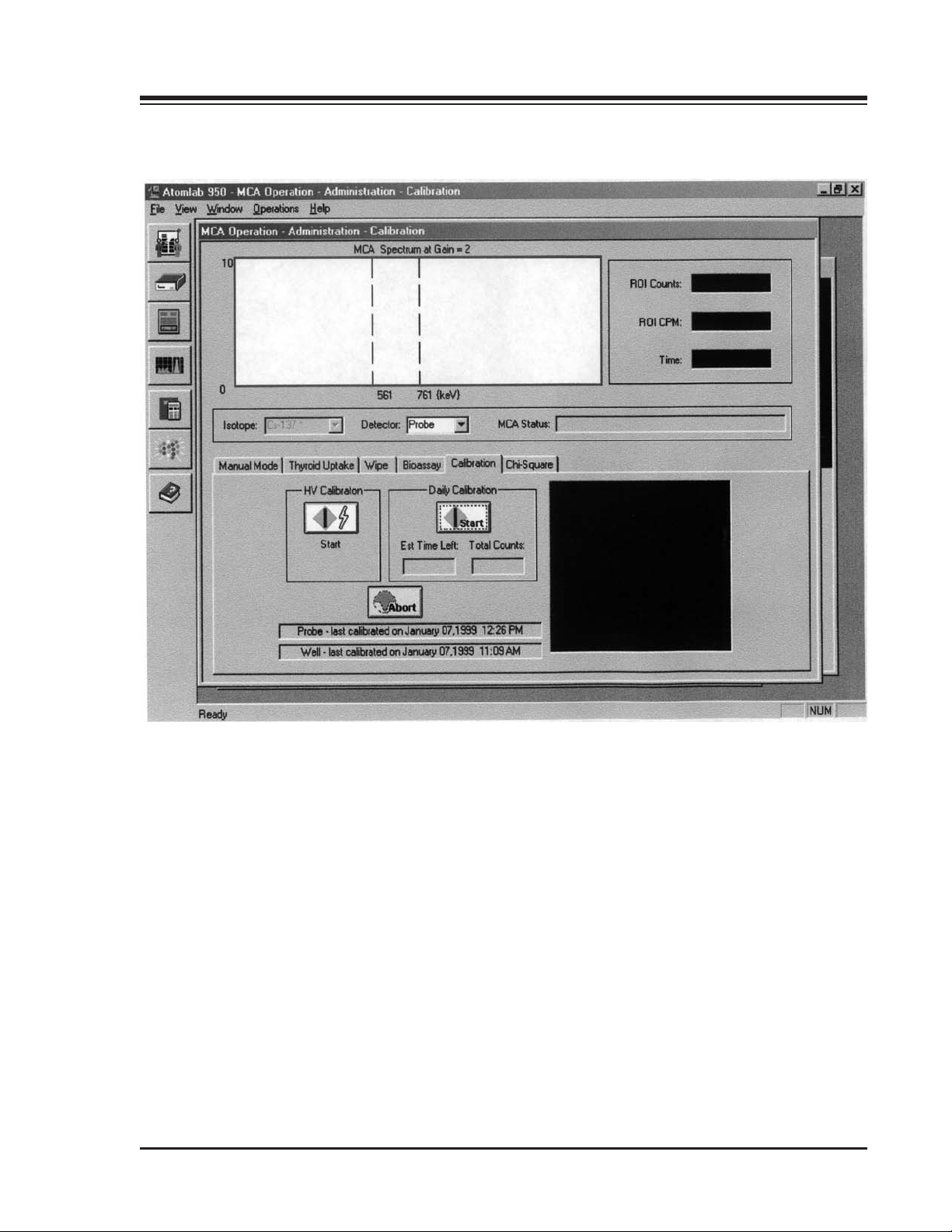
(See Figure 3-1and 3-2.)

NOTE: The system must be ON for at least one hour before performing a calibration. This will allow time for the
unit to warm-up and stabilize.

Calibration Information

A daily system calibration must be performed each day the Atomlab 950 is to be used. Separate
calibrations are performed for the probe and well. The system keeps an internal listing of its last
calibration date and displays a message that calibration is needed. The user must then either perform a
calibration or click on the prompt that a calibration will not be performed. The system will not allow
measurement procedures to commence until the calibration prompt has been answered. Standard
calibration may be performed from any operating mode.

Calibration is performed automatically from the MCA Calibration screen. This screen advises when the
last high voltage and calibration were performed for your detectors. It also checks to ensure that the MCA
box and CPU are connected and communicating with each other.

Additionally, the calibration calculates full width half max (FWHM). FWHM is determined by
interpolating between two immediate points above and below the 50% value of the spectrum peak on
both sides of the peak. The difference between the two interpolated channel numbers are then divided by
the channel of the peak itself and multiplied by 100% to arrive at FWHM. The peak is simply the
maximum value in the spectrum.

It is not required to calibrate both detectors each day unless you are going to use them. If you do not
calibrate the detector when you go to use that detector, you will get a message advising you to calibrate.
It is recommended to do your calibrations in the mornings daily so that if you need to use the system, it is
ready to go.

If desired, you may perform additional calibrations on the same day whenever you desire by clicking on
the <Calibration> mode tab.

While the daily calibration is counting, in the upper right you see the ROI counts incrementing and the
CPM incrementing as well. The elapsed time is shown next to the time button. Below the start button is a
box listing estimated time left. This gives the remaining time to complete the calibration. The spectrum
increments as you count as the packets with the data are downloaded to the computer from the MCA.
The <Abort> button is highlighted and is the default button used in this mode at this point. You will

3-1 ADMINISTRATION

1. INTRODUCTION

notice a dotted line around <Abort>. This means that by pressing the space bar it will automatically stop
and you do not need to move the pointer to that pointer. The <Abort> button stops the system from
counting and also will not retain the information that has been counted during this function.

When the system finishes counting in the upper right you will see what looks like a MCA box sending
information to the computer pictorially. This means that a final download of information is being sent.
After the information is sent, a screen is displayed listing the full width half max (FWHM), the energy in
the peak channel. If this is acceptable click on <Accept> in the pop-up window. If you do not want to
accept it, press <Cancel>.

Both daily calibration and Chi-Square tests are performed using a 10 µCi Cs-137 button source. Once
calibration is underway, the system's unique differential spectrometer automatically measures the peak
height and subtracts the base line - which makes zero adjustment obsolete. It does this for 100,000 pulses
and then plots a spectrum in internal memory. The peak channel is located and equated to 662 keV,
which is the Cs-137 gamma entered. This gives the spectrometer the keV per channel which is used to
calibrate all of the other isotope gains. Each clinical isotope has a ROI defined with lower and upper
energy limits. These energy limits are then converted to channels in the MCA when a particular isotope is
counted. Corrections are made for sodium iodide NaI non-linearity. There is no need to view the
spectrum of calibration or any other isotope, although this is available on the display and in hard copy by
selecting the spectrum icon.

The multi-channel analyzer in the Atomlab 950 has several fixed precision gains and a regulated high
voltage supply. The pulse shapes are digitized and then processed by a high speed digital signal
processor. This processing results in a possible 1024 pulse heights which has zero offset. A spectrum
results when a histogram of these pulse heights (channels) is plotted. Calibration of the spectrometer is
defined as knowing the energy equivalence of each channel. This is accomplished by determining the Cs­137 spectrum and then calculating the ratio of the 662 keV/peak channel. After calibration, the report
should always print a peak value very close to 662 keV (some precision round-off may occur), and the
change in calibration will be reflected in the keV/channel slope value. The fine gain can be thought of as
a floating point numerical gain. The HV adjust will ultimately determine the maximum energy one can
measure on the gain selected. It can be calculated by multiplying the keV/channel times 1024.

To Perform a Daily Calibration

1. After the system has been turned ON for at least one hour, select <Calibration> from the Operation
screen. The Calibration menu is now displayed on the screen. Select well or probe in the detector
window.

2. Position the 10 µCi Cesium-137 source approximately six inches in front of the appropriate detector.

3. Click on <Start> daily calibration.

4. The display will tell you that probe calibration is in progress. If calibration is successful, click on
<Accept>. Click on <Ignore> to discard the calibration without saving.

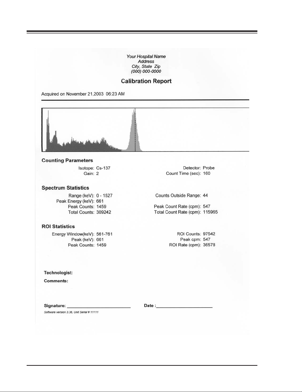
5. After accepting the calibration, you can print a report by clicking on the <Report> icon in the
primary tool bar at the left of the screen.

6. In the Report window you can enter the technologist's name and any comments required for these
reports. To review the report, click on <Preview>. To print the report, click on <Print>.

7. The printer page will now be displayed. If the correct printer is indicated, you can select multiple
copies or, for some reports, the number of the page you want to print.

NOTE: If youjustclick <Print> thecalibration pagesfor both the well andprobe willbeprinted.Ifyou onlyperformed the
calibrationon onedetectorand only wanttoprint thatdetector,youmustindicatethatonthe print page.Thisisdoneby
adjusting theprint rangefromAll toPages (fromXXto XX). Youcan printat anytimethe latest calibrationscreens foreach
detector.

ADMINISTRATION 3-2

CONTENTS

Figure 3-1. The Calibration Screen.

3-3 ADMINISTRATION

1. INTRODUCTION

Figure 3-2. A Calibration Report.

ADMINISTRATION 3-4

CONTENTS

Calibration Screen Description

Multi-channel analyzer display: This display has a scale on the left side showing counts full scale. On the
bottom is the scale that shows the ROI.

ROI Counts: To the right of the MCA display is a box showing ROI counts for region of interest counts,
ROI cpm and time. The time is the time that the system is counting.

Isotope: The isotope in this box is the one displayed above as the region of interest. This is the isotope for
which the system will count.

Detector/Well: To the right of the Isotope is a box showing the active detector or well. To display the
available detectors or wells, place the cursor over the small arrow in this box. If you would like to change
the detector or well, click on the desired detector or well to select. The new detector will now be
displayed in the Detector box.

MCA Status: This box provides notes about what is happening at the current time. It will tell you when
counting is in progress or that information is being downloaded from the MCA box to the computer as
well as a number of other informational items.

Modes of Operation: Below the MCA Status box are tabs for the different modes of operation. These tabs
include Manual Mode, Thyroid Uptake, Wipe, Bioassay, Calibration and Chi-Square.

Mode or Function Specific Counting: Below MCA Status box is Mode or function-specific counting
information. Each mode has a <Start> button. Clicking on <Start> immediately begins the counting. The
<Abort> button is used to stop counting without storing the data. The <Stop> button stops the MCA
from counting but continues to use the information gathered in the program in which you are working.

High Voltage Adjustment should be performed the very first time the system is used, if the system is to
be used in a new environment or in the instance where a substantial change has been made, i.e., when
using a new tube.

NOTE: If a probe and well are both used the high voltage adjustment must be set independently for each detector.
The system must be ON and warmed-up prior to setting the high voltage.

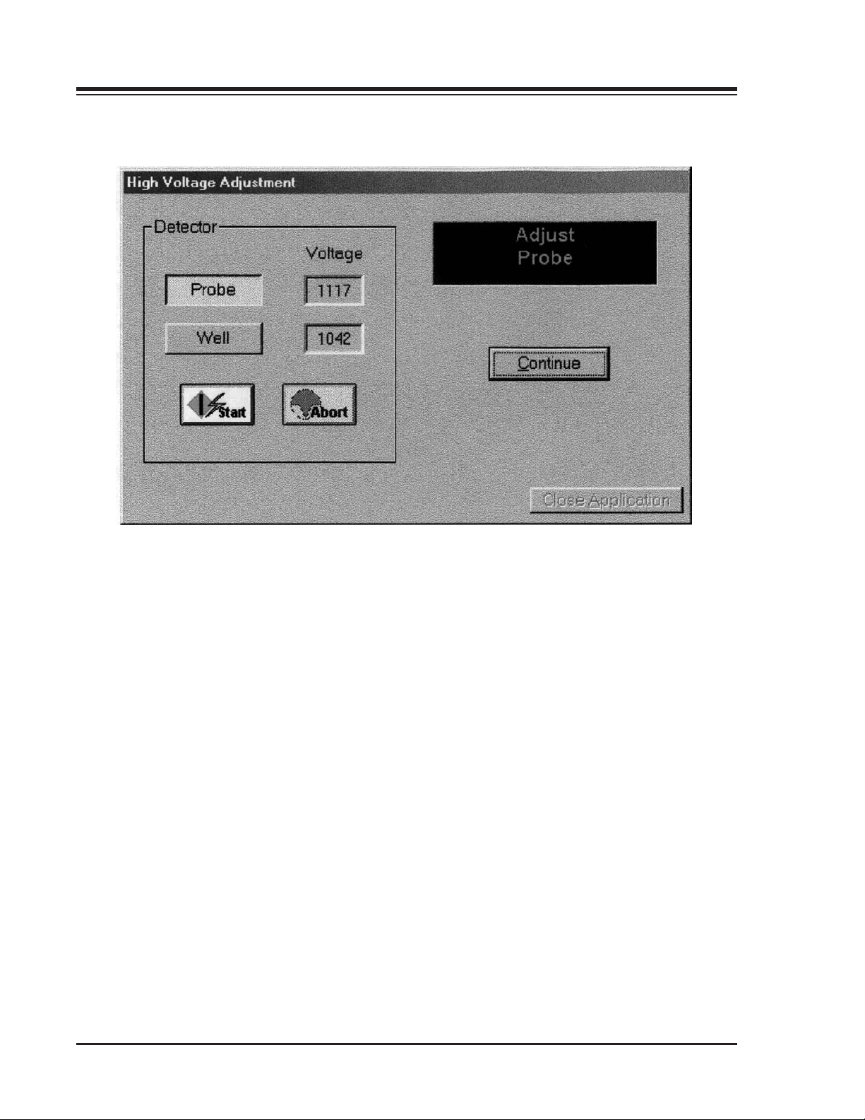
High Voltage Adjustment

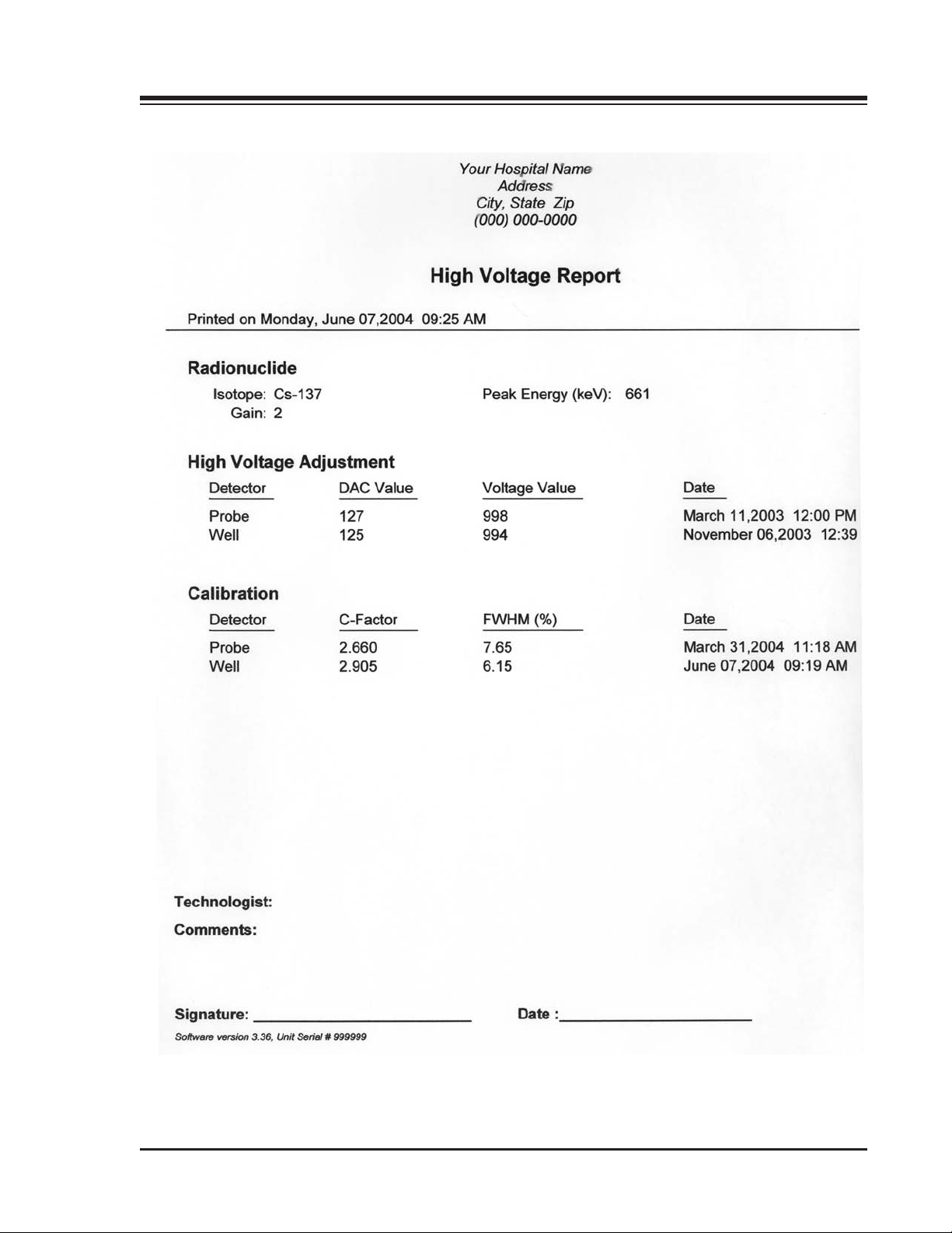
(See Figure 3-3 and 3-4.)

To Perform a High Voltage Adjustment

NOTE: When a High Voltage Adjustment is performed on a detector, the previous calibration and Chi-Square for
that detector are zeroed. You must perform a new calibration and Chi-Square for a detector following a High
Voltage Adjustment. You can do a High Voltage Adjustment for either detector at any time.

1. From the Operation screen, click on <Calibration>. The Calibration screen should now be displayed.

2. Click on <HVAdjustment> to access the High Voltage Adjustment counting screen.

3. Click on the appropriate detector.

4. Click on <Start> to perform the High Voltage.

NOTE: If you do not want to perform a High Voltage, click on the <Continue> and the system will return to
the Calibration page.

3-5 ADMINISTRATION

1. INTRODUCTION

Figure 3-3. The High Voltage-Adjustment Screen.

ADMINISTRATION 3-6

1. INTRODUCTION

Figure 3-4. The High Voltage Report.

3-7 ADMINISTRATION

1. INTRODUCTION

5. Once a High Voltage Adjustment is started, it will run until it is completed unless you choose to
abort. When it is completed, the system will inform you and then shift to the other detector to allow
you to do another high voltage adjustment if desired.

6. Click on <Continue> to return to the Calibration page.

NOTE: If you have started a high voltage adjustment and wish to stop, click <Abort>. This will stop the
count. Click <Continue> to return to the Administration page.

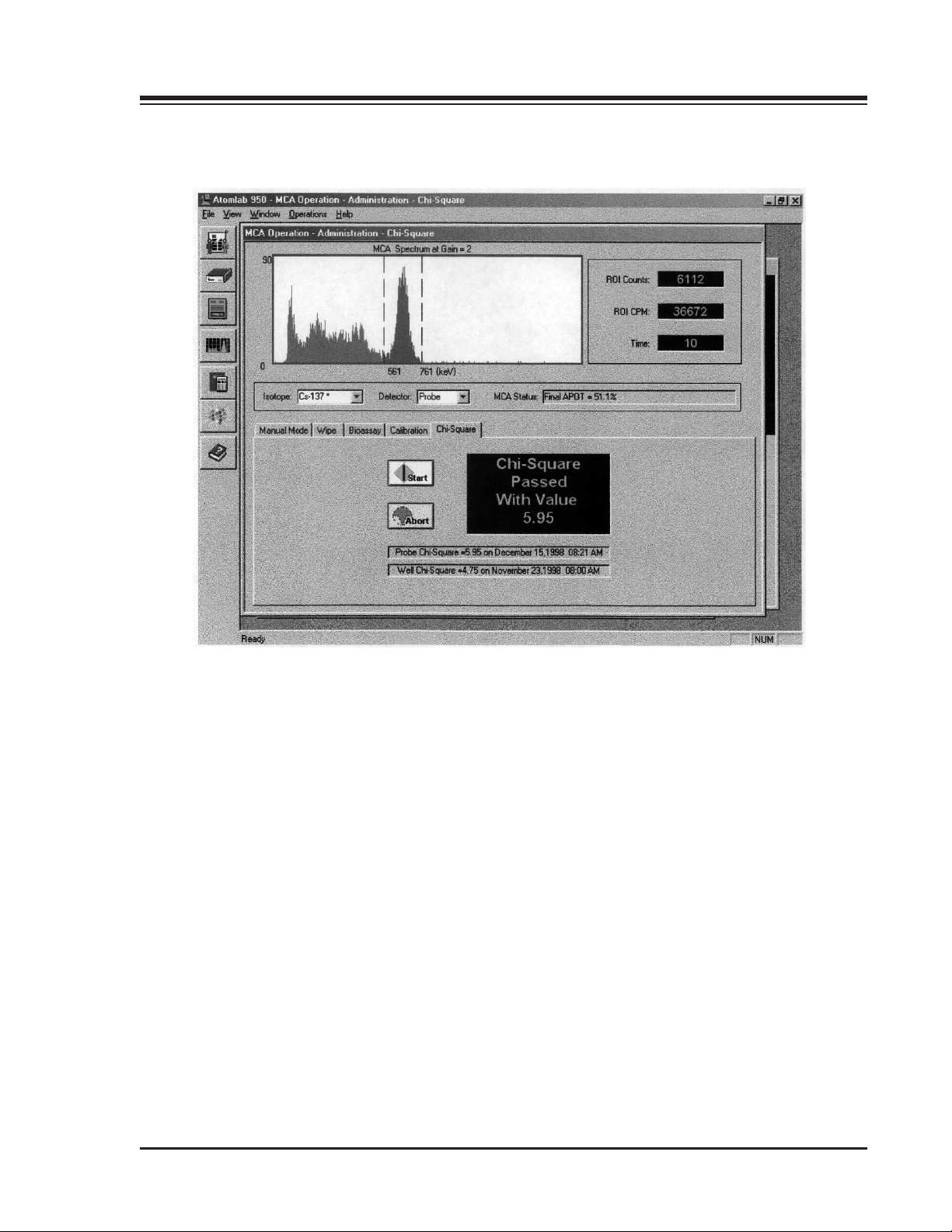
Chi-Square

(See Figures 3-5 and 3-6.)

As is the case with Daily Calibration, Chi-Square is performed using a 10 µCi Cs-137 button source. The
Chi-Square Test is independent of the counting time, counting rate, and number of counts performed. For
this reason, Chi-Square is a very valuable test for a detector system which is recording truly random
events. For example, if systematic failure occurs at low counting rates but passes at high rates, there is an
indication of a non-random event occurring which is comparable to the low counting rates. Since time is
precise to within 10 microseconds with a crystal controlled clock, 10 second count times should have very
little error due to the timer itself.

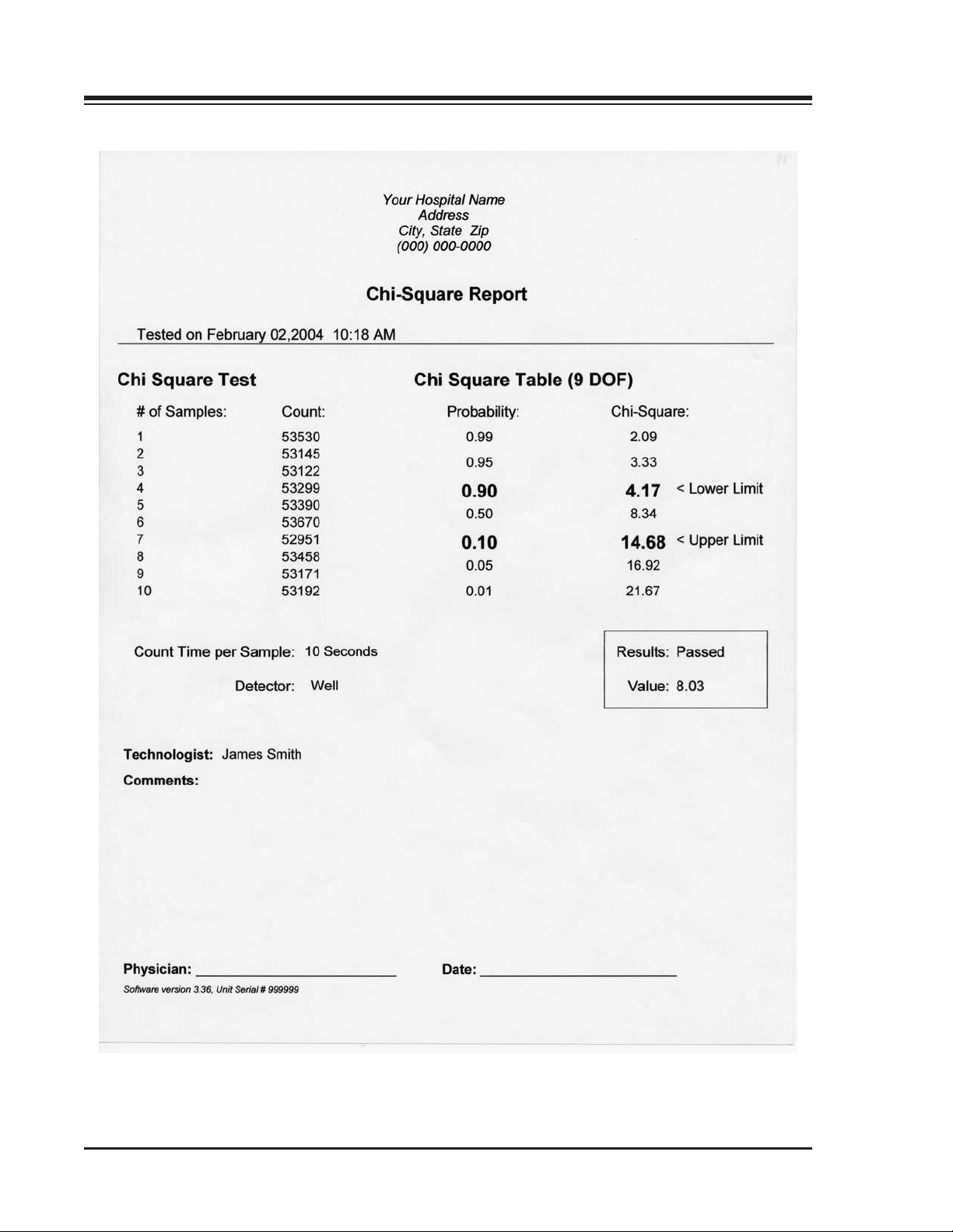
The number of counts performed is 10, which determines the number of degrees of freedom (9) for the
analysis. The lower limit is 4.168, the upper limit is 14.68. These correspond to a 90% probability for
passing the lower limit, and 10% probability for passing the upper limit, respectively. In all, one would
expect a 20% failure rate frequency for the Chi-Square test. It is not reasonable to always pass or always
fail Chi-Square without raising concerns that there may be a systematic problem in the detector or
counter.

NOTE: The system stores the information for the latest Chi-Square test performed on a detector. Chi-Square can be
performed as frequently as desired, but is generally performed quarterly.

To Perform Chi-Square

1. Click on the <Chi-Square> tab in the center of the Calibration screen. This brings up the Chi-Square

screen.

2. Select the detector on which to perform a Chi-Square. The arrow in the detector box will bring up

your choice of detectors. Highlight the appropriate detector and proceed.

3. Position the 10 µCi Cesium source in front of the appropriate detector. Click on <Start> and the

system will automatically perform a Chi-Square test on the selected detector.

4. The system will display the elapsed time and the pass number that is currently being counted. The

pass number is the sample number currently in progress. The system will automatically increment
until all 10 passes or samples have been counted. At the completion of the 10th pass the system will
calculate Chi-Square and display the value on the screen, along with a passed or failed note. At this
point the result is entered into the system memory.

5. You can print out a Chi-Square report by clicking on the <Report> icon in the primary tool bar and

then choosing Chi-Square.

6. If desired, enter the technologist and any comments you want printed with the report. To review

what is going to be shown, click on <Preview>. To just print, click on <Print>. In print the default is
ALL, which will print the latest Chi-Square reports for both well and probe. If you only performed
one Chi-Square at this time, highlight pages from 1 to 1 for probe, or from 2 to 2 for well only.

ADMINISTRATION 3-8

1. INTRODUCTION

Figure 3-5. The Chi-Square Screen

3-9 ADMINISTRATION

1. INTRODUCTION

Figure 3-6. The Chi-Square Report.

ADMINISTRATION 3-10

CONTENTS

7. Click <OK> and the report will automatically print. The system returns to the Report Generation
screen from which you can print another report if you like. To close the Report Generation screen,
click on the <Close> icon.

A sample Chi-Square counting screen is shown as well as a Chi-Square printed report.

Administration Report

(See Figure 3-7.)

Following daily calibration, Chi-Square, or High Voltage, the user can print an Administration Report
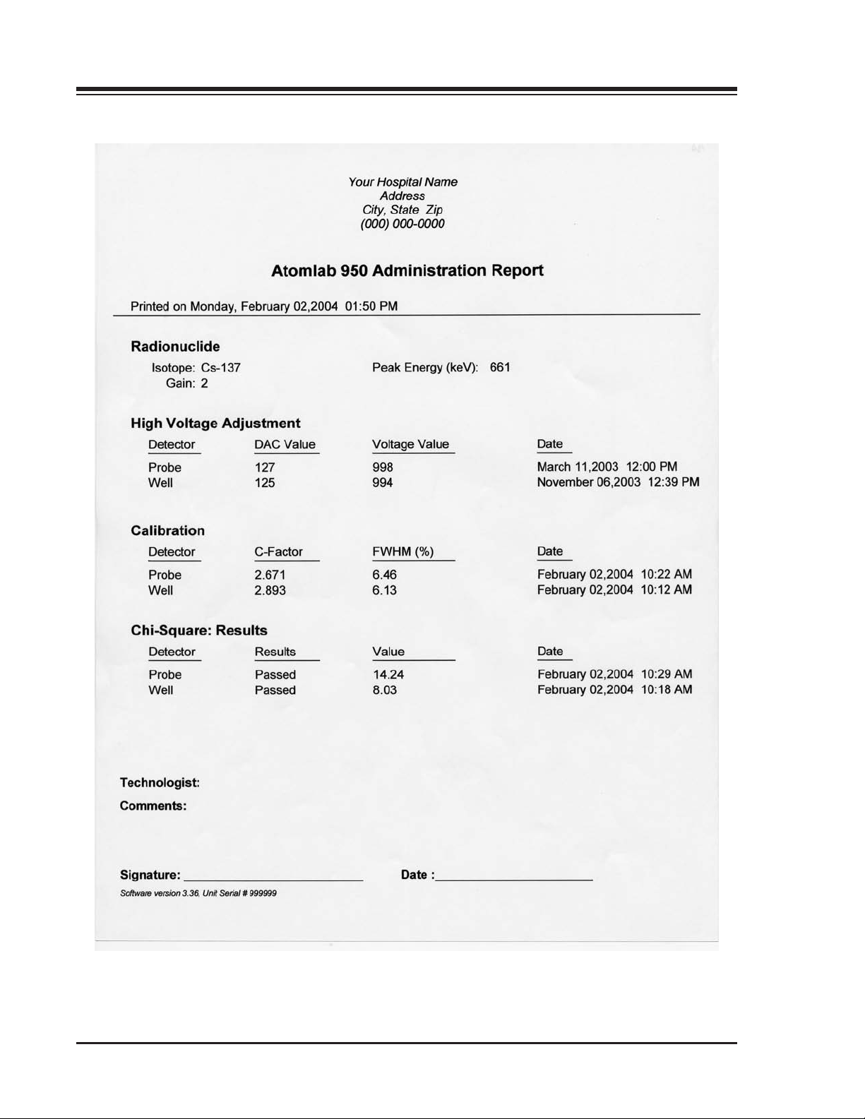
showing the High Voltage Value, Calibration Factor full width half max (FWHM), most recent Chi­Square results, the person performing the calibration and comments. This report can be printed anytime.

To Print An Administration Report

1. Click on the <Report> icon in the primary tool bar.

2. Choose <Administration Summary>. You can enter a technologist and comments. If you desire to
look at the report before printing, click on <Preview>.

3. Press <Print> to print the report. This brings up the printer screen.

4. Click on <OK> to print.

NOTE: The High Voltage Report and the Atomlab 950 Administration Report are similar. The Atomlab 950
Administration Report includes Chi-Square results, the High Voltage Report does not include the Chi-Square
results.

Isotope Editing

(See Figures 3-8, 3-9.)

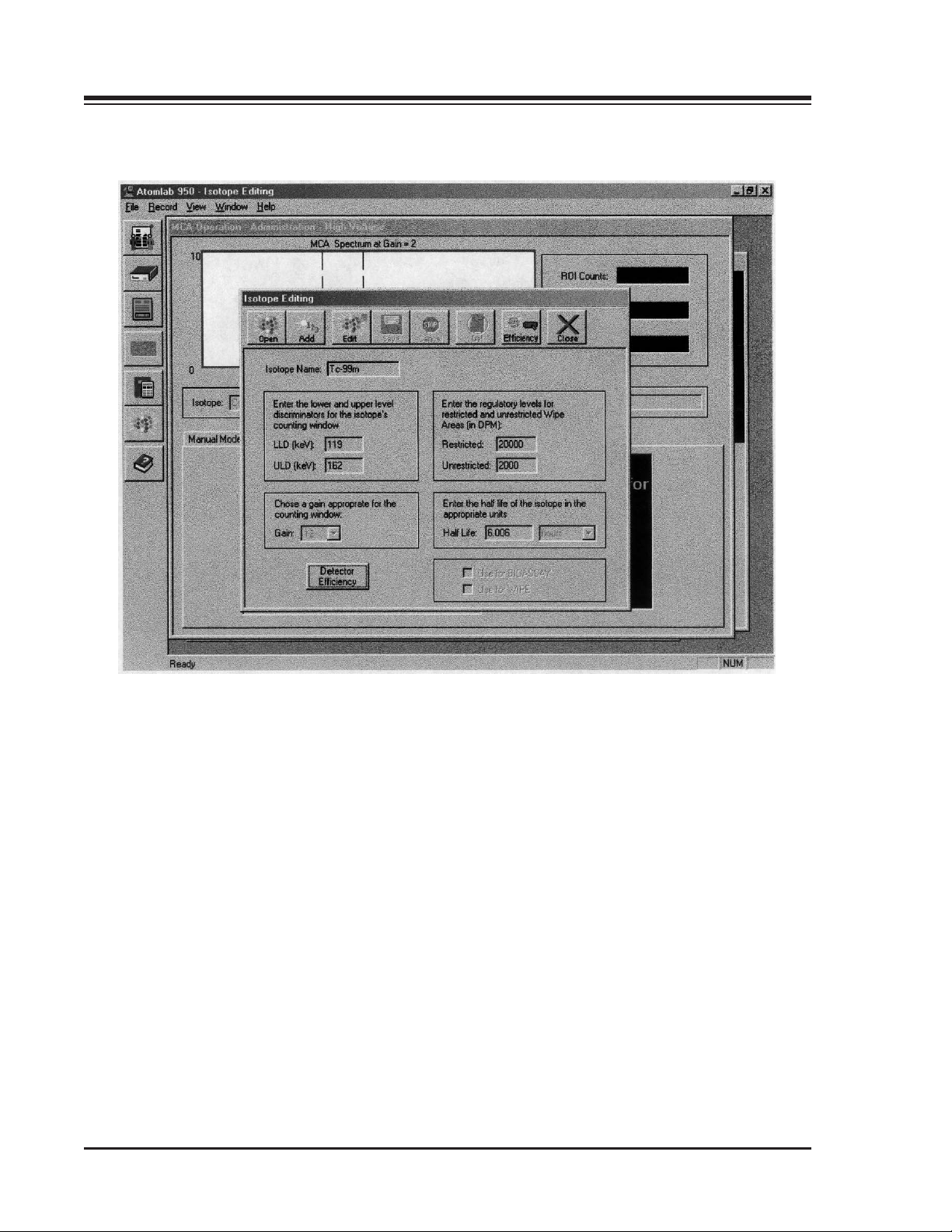
This option allows the user to select and view a preset isotope, add a new isotope to the isotope list, edit
an existing user-entered isotope, and activate an isotope so that it can be used for Bioassay or Wipe
functions.

The Atomlab 950 isotope list comes with 23 preset isotopes. For these factory isotopes, Lower Level
Discriminator (LLD), Upper Level Discriminator (ULD), regulatory alarm levels and Gain are factory
preset and cannot be changed. For all user entered isotopes, LLD, ULD and Gain can be edited.

While this option is active, the currently selected isotope is always highlighted in the isotope name at the
top left of the page.

NOTE: Placing a checkmark in the <Use For> field at the bottom right of the screen allows the selected isotope to be
used for Bioassay or Wipe. If you do not check the <Use For> fields the isotope will be unavailable for these
functions. Once you have checked the appropriate function(s), add a detector efficiency as described later in this
chapter.

To Select a New Isotope

1. Click on the <Isotope> icon in the primary tool bar. The Isotope Editing screen should now be

displayed.

2. The Isotope Editing screen displays information about the currently selected isotope. Click on

<Close> to keep the currently selected isotope and return to the Main Menu.

3-11 ADMINISTRATION

1. INTRODUCTION

Figure 3-7. An Administration Report.

ADMINISTRATION 3-12

CONTENTS

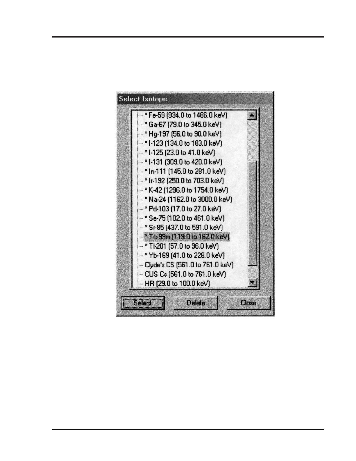
3. To select another isotope from the Isotope Editing screen, click on <Open>. A list of isotopes will be

displayed.

4. Highlight the desired isotope from the Isotope List and click <Select>. The new isotope is now

displayed in the Isotope Name box. All information on the Isotope Editing screen now reflects the
new isotope.

To Add or Modify a New Isotope

Adding an isotope is most easily accomplished by modifying an existing isotope from the Isotope List.
(For example, if you want a wider window for Technetium then the factory preset value, modify
Technetium on the Isotope List so that it has a new name such as "Technetium Wide." You can then
modify the upper and lower level discriminators.)

1. Click on the <Isotope> icon in the primary tool bar. The Isotope Editing screen should now be

displayed.

2. Click on <Open>. The Isotope List should now be displayed.

3. Highlight the desired factory isotope to modify from the Isotope List and click <Select>. The new

isotope is now displayed in the Isotope Name box. All information on the Isotope Editing screen
now reflects the new isotope.

4. Click on <Add>.

5. Enter a custom name for the new isotope and modify the specifications as required.

6. Once all modifications are complete, click <Save> at the top of the isotope menu. If you do not wish

to save what you have entered or want to get out of this screen, click <Cancel> to exit without
saving.

To Edit An Isotope

With the Isotope Editing Screen displayed, clicking on <Edit> allows you to change information
associated with the currently selected isotope. For factory isotopes, you can adjust only detector efficiency
or whether to use it for Bioassay or Wipe.

For custom isotopes editing allows for adjustment of area readings, half-life gain, ROI settings, as well as
the isotope name.

1. Click on the <Isotope> icon in the primary tool bar. The Isotope Editing screen should now be

displayed.

2. Click on <Open>. The Isotope List should now be displayed.

3. Highlight the isotope to edit and click on <Edit>.

4. Make the appropriate changes to the isotope you are editing.

5. Once you have made the edits desired, click <Save> to save the edited isotope.

3-13 ADMINISTRATION

1. INTRODUCTION

Figure 3-8. The Isotope Editing Screen.

ADMINISTRATION 3-14

1. INTRODUCTION

Figure 3-9. The Select Isotope Window.

3-15 ADMINISTRATION

CONTENTS

To Delete an Isotope

Only custom isotopes can be deleted from the Isotope Editing screen. Factory set isotopes cannot be
deleted.

1. Click on the <Isotope> icon in the primary tool bar. The Isotope Editing screen should now be
displayed.

2 Click on <Open> The Isotope List should now be displayed.

3. Highlight the isotope to delete.

4. Click on <Delete>. The system will ask if you really want to delete the selected isotope. Click <Yes>
to delete or <No> to abort. The system will now return to the Isotope Editing screen. If you have
deleted a custom isotope it will no longer show on the Isotope list.

Isotope Report

Isotope Reports can be generated showing all the parameters for individual isotopes or listing all the
isotopes. These printouts can be accessed by selecting the <Report> icon in the primary tool bar.

Isotope Efficiencies

(See Figures 3-10 and 3-11.)

All efficiencies are set to zero as shipped from the factory. The user has the choice of either calculating the
efficiencies to be used or using the analytically determined factory defaults.

NOTE: The total efficiency for an isotope using the system is the Geometric efficiency times the detector efficiency .
See Apendix A for more details.

NOTE: An isotope will not be available for use for Wipe Testing or Bioassay unless an efficiency has been set to
other than zero.

Setting Geometric Efficiency

The geometric efficiency for the system is independent of the isotope being used. The geometric efficiency
refers to the placement of the isotope in relation to the detector.

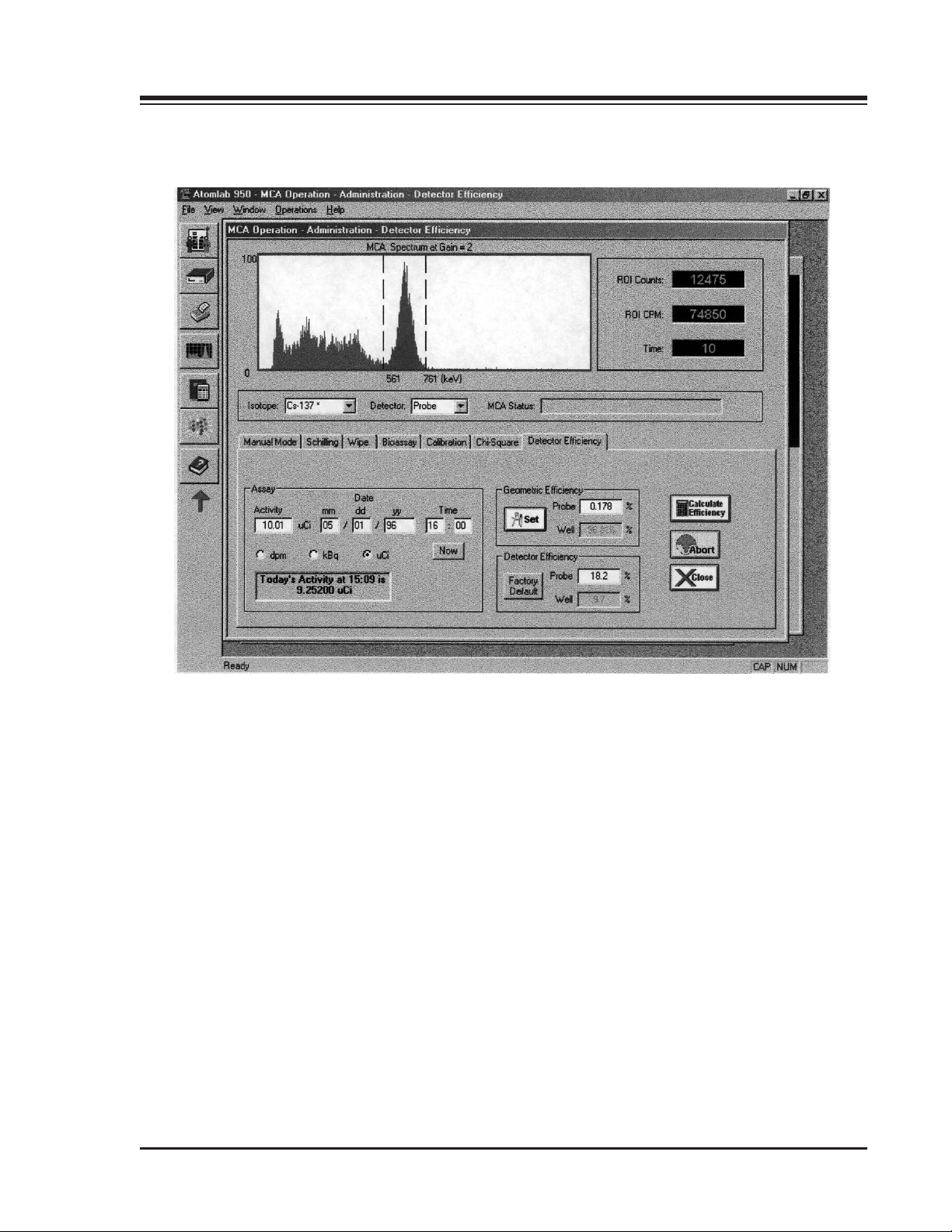
1. From any screen, click on the <Isotope> icon in the primary tool bar. The Isotope Editing screen
should now be displayed.

2. Click on <Efficiency> in the screen tool bar. The Detector Efficiency screen should now be displayed.

3. Click on <Set> in the Geometric Efficiency box and then select either well or probe. You can now
enter information concerning the selected detector.

NOTE: If you select probe, you would enter the outside diameter of the detector and the distance from the
probe. This uses a formula described in Appendix A under Isotope Efficiency Calculation. You must enter the
same unit of measure for both of these numbers. It is suggested to use centimeters for these as there is a cm
scale for distance from the face of the detector on the collimator. The factory preset for the outside diameter is

5.08cm, which is the 2-inch diameter detector. The distance from the probe is the distance from the end of the
distance bar to the face of the crystal. For the well it is the inside diameter, which on the well shipped by
Biodex, is 1.905cm. Factory set well depth is 2.54cm. This depth in the well would be indicative of many wipes
where the center of the activity or where the wipe would be located when lowered into the well. This would be
the depth from the top of the crystal, not from the top of the lead of the collimator.

4. Once you have set the desired numbers, click <OK> to return to the Detector Efficiency screen. If a
different efficiency than the one you desire is displayed on the Detector Efficiency window, double
click on the box next to the appropriate detector and type in the efficiency you desire.

ADMINISTRATION 3-16

1. INTRODUCTION

Figure 3-10. The Detector Efficiency Screen.

3-17 ADMINISTRATION

CONTENTS

DETECTOR EFFICIENCY

To Enter A Detector Efficiency

1. From any screen, click on the <Isotope> icon in the primary tool bar. The Isotope Editing screen will
be displayed.

2. Click on <Detector Efficiency> at the bottom of the screen. The Detector Efficiency screen will be
displayed.

3. At the Detector Efficiency screen, double click on the box next to the appropriate detector and key in
the new detector efficiency value. The value entered will be the efficiency used for the isotope
indicated in the isotope window. Each isotope must be set individually for an isotope efficiency.

NOTE: If the efficiency is less than one (1), it must be entered in decimal format (i.e., 0.1, 0.2, etc.)

4. Click on <Close> to return to the Isotope Editing screen.

To Select a Factory Default Detector Efficiency

NOTE: The following procedure is for selection of a factory default detector efficiency which was obtained using an
analytical approach to efficiencies for a sodium iodide detector.

1. From any screen, click on the <Isotope> icon in the primary tool bar. The Isotope Editing screen will
be displayed.

2. Click on <Detector Efficiency> at the bottom of the screen. The Detector Efficiency screen will be
displayed.

3. Highlight the appropriate detector and the appropriate isotope.

4. Click on <Factory Default>.This will place the analytically determined factory default value into the
appropriate detector window.

5. Click on <Close> to return to the Isotope Editing screen.

To Calculate a Detector Efficiency for a Specific Isotope

1. From any screen, click on the <Isotope> icon in the primary tool bar. The Isotope Editing screen will
be displayed.

2. Click on <Detector Efficiency> at the bottom of the screen. The Detector Efficiency screen will be
displayed.

3. To calculate a detector efficiency for a specific isotope, a sample of the activity with a known
calibration date and time must be prepared. Enter this activity (preferably in microcuries) in the
assay window at the bottom left of the Detector Efficiency screen.

NOTE: If the activity is less than one (1), it must be entered in decimal format (i.e., 0.1, 0.2, etc.)

4. Enter the date and time of calibration of the standard. Today's activity at the current time is shown
in the window below the assay window.

NOTE: Click <Now> to instantly make current the date and time for the activity shown. This is convenient if
you are making up a standard which you wish to count. You can then adjust from the current time to the
calibration time of your standard.

ADMINISTRATION 3-18

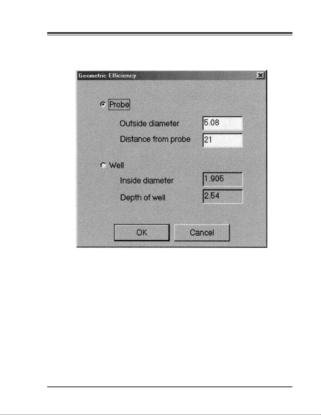
1. INTRODUCTION

Figure 3-11. The Geometric Efficiency Window.

3-19 ADMINISTRATION

CONTENTS

5. Click <Calculate Efficiency>. A window will be displayed telling you to prepare to count
Background. Ensure there are no isotopes in the area before you click <OK>.

6. Once you click on <OK>, the system will proceed to count for 100 seconds. When it is done
counting, a menu will be displayed telling you to place an isotope at the proper distance from the
detector and to click <OK> when ready. When you click <OK> this time, the system will again start
counting for the isotope for a 100 second time frame. When the system has finished counting for 100
seconds, calculated detector efficiency for this isotope will be displayed starting with the activity
that you have entered.

Decayed Activity

To determine the decayed activity of a source: (For example, the current activity of a sealed Co-57 source.)

1. Open the Detector Efficiency page.

2. Select the desired isotope by clicking on the <down arrow> and selecting the desired isotope.

3. In the Assay window, click on either <Bq> or <µCi>.

4. Enter the calibration time and date for the source.

5. Enter the activity at the time of calibration.

6. In the window at the bottom of the screen you’ll see listed “Today’s Activity at the current time
is _______.”

SPECTRUM ANALYSIS

(See Figures 3-12 and 3-13.)

Spectrum Analysis is available in any operational mode throughout the program. This option allows the
user to change the ROI on the display, add additional ROI's, or print the spectrum with counting
information.

To Access The Spectrum Analysis

1. Click on <Spectrum> in the primary tool bar. The Spectrum Analysis screen should now be displayed.

The spectrum from the immediately preceding count is shown with its associated data. On the
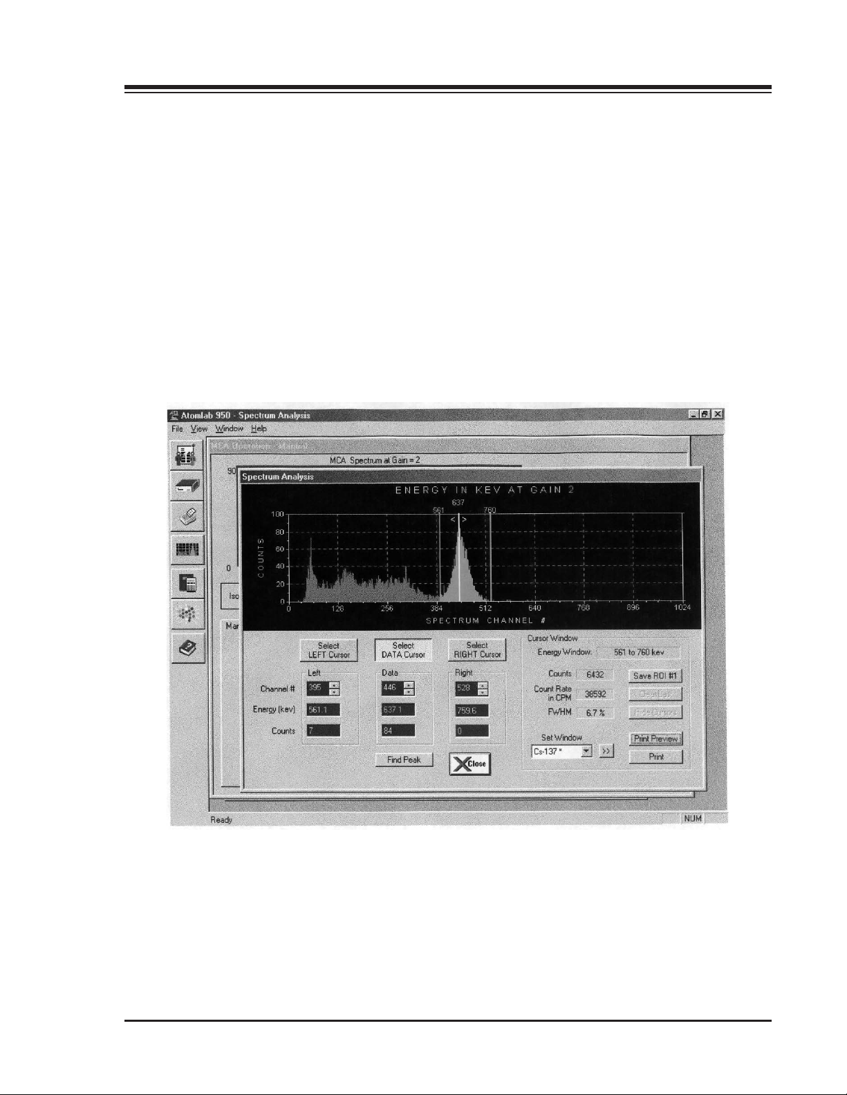
Spectrum Analysis screen, the ROI for the isotope counted is shown on the screen. The set window
for that isotope is displayed in the bottom of the Cursor Window. The left channel is shown in the
Select Left Cursor box while the right channel is shown under the Select Right Cursor box. The Select
Data Cursor is your cursor that can be moved.

2. To move any ROI or cursor, click on the box for the appropriate line and then use the <Up> or
<Down> arrows under the cursor. As you move the cursor, the energy and counts associated with
that channel will change.

• On the right hand side of the screen, the cursor window shows the energy between lower and

higher keVs set by the ROI shown to the left.

• The counts are the counts in that region of interest. The count rate is the rate in the region of

interest that the cursor is in, displayed in cpm.

• The full width half max (FWHM) is displayed for the appropriate peak in that window.

ADMINISTRATION 3-20

1. INTRODUCTION

3. To choose a different isotope, click on Set Window and highlight the desired isotope from the
isotope list. The window will switch to that keV setting and display it.

NOTE: The >> button to the right of the Set Window can be used to cycle through the isotope list while
displaying the regions of interest for all the factory and custom isotopes that are stored in memory. This can
help identify an unknown peak that is on your display. If you use this feature to go to a lower gain isotope, the
system may display a message that the lower limit of deection of Co-58 is above the window limit of the selected
gain. This message will be displayed for each isotope until you select one that has an acceptable gain. Click on
<OK> to remove the message window and select another isotope.

4. To set multiple regions of interest on the screen, click on <Show/Hide Cursors> in the Cursor
Window. You can now click on <Select Left Cursor> or Select Right Cursor> and move the cursor to
the desired point. Use the <Up> and <Down> arrows to refine this setting.

Figure 3-12. The Spectrum Analysis Screen.

3-21 ADMINISTRATION

1. INTRODUCTION

5. To find the peak in the ROI, click on <Find Peak>. Click on <Save> to save this second region of
interest as ROI #2. To create additional regions of interest, click on <Show Cursors> and repeat steps
4 and 5.

6. To print a Spectrum Analysis Report, click on <Print Preview> at the bottom right of the Cursor
Window for a preview. To print the report, click on <Print>.

7. To exit Spectrum Analysis, click on <Close> at the bottom center of the Spectrum Analysis screen.

How is ROI Determined?

The preset ROI energy window values do not change as the user switches between well or probe,
regardless of the mode selected (i.e., Uptake, Schilling, MCA, etc.). The ROI is defined in units of energy
(keV) and then converted to channel numbers with the keV/channel slope value that is measured during
calibration. The channel number for the ROI values can and will change from probe to well if the
calibration keV/channel is different between probe and well.

Example

Tc-99m has a peak energy of 140 keV according to the radionuclide decay scheme. The Atomlab 950 uses
a default of +/- 15% energy window around the peak energy. These values calculate to be 119 keV to 162
keV and are displayed on the Isotope Editing page. When either the probe or well is selected, the ROI
channels are calculated based upon the Cs-137 calibration results for that particular detector. If the
calculation of the probe results in a .3775 keV/channel on gain 8, the TC-99m default gain, the channel
ROI will be 119 keV/.3775 keV channel = channel 315 and 162/.3775 = channel 429. For the well detector,
we might have a calibration of .3325 keV/channel. In this case, the ROI channels will calculate channel
358 to 487. Even though the ROI channels are different, the energy windows are the same. This will
become apparent when the spectrum for each detector is printed.

NOTE: It is not necessary to fix a symmetrical percent around the peak. In fact, some isotopes are multi-peaked,
which can cause an asymmetric spectrum. Keep in mind that if a calibration is performed you must save the result
in order to have it used in ROI calculations.

If you select an isotope from the Isotope Editing page, the screen will display the isotope name, LLD,
ULD, and gain setting as demonstrated in the following chart.

Gain Max keV Half Scale
1 3000 1500
2 1500 750
4 750 375
8 375 187
12 250 125
48 64 32

A. Lower Level Discriminator (LLD) = 0.85 times the Min keV of interest.
B. Upper Level Discriminator (ULD) = 1.15 times the Max keV of interest.

ADMINISTRATION 3-22

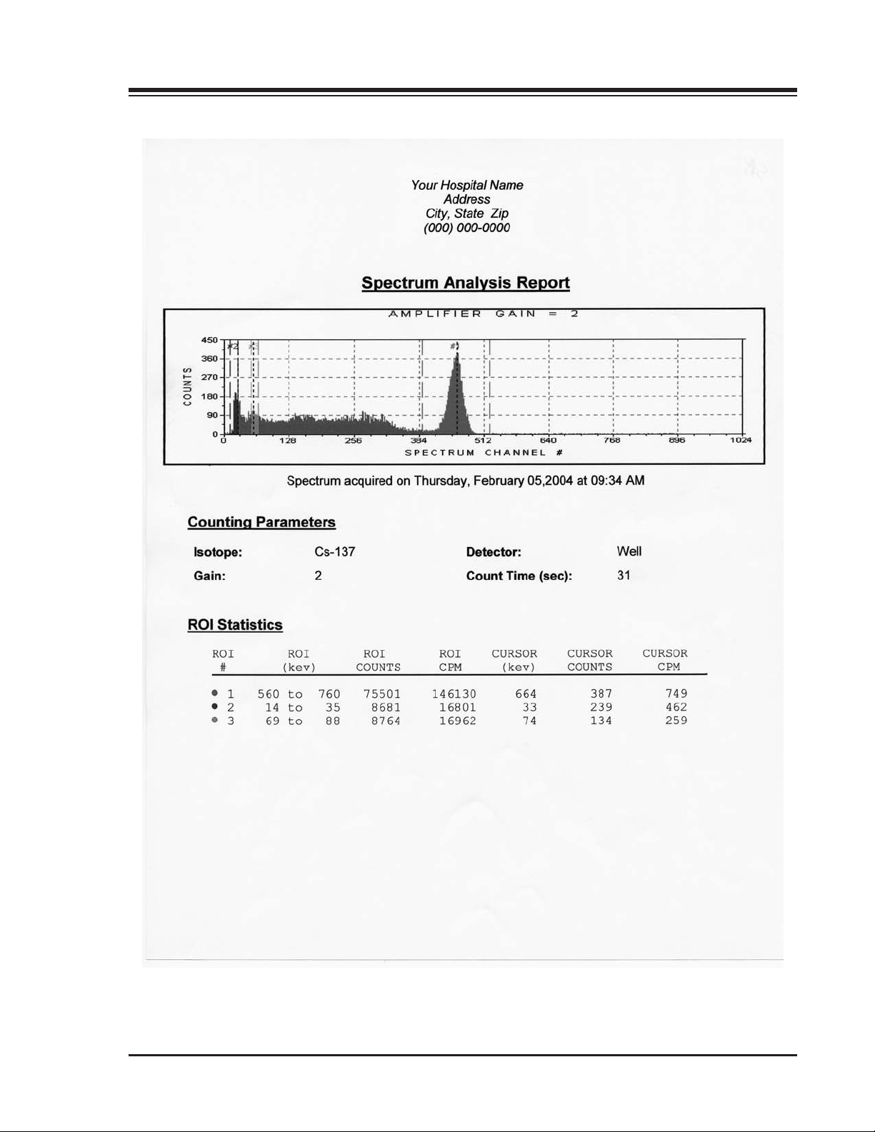
1. INTRODUCTION

Figure 3-13. A Spectrum Analysis Report.

3-23 ADMINISTRATION

4. THYROID UPTAKE

In this mode, a radioactive uptake study is performed. The system guides the user through a step-by-step
procedure that includes counting the following: standard, lab background, patient thyroid, patient
background, and finally the computation of the uptake percentage. The uptake percentage, which is
calculated from an automatically decay corrected dose count or recounted standard, can then be printed
in a format designed to provide complete information on the patient study.

The system allows multiple data sets for different times for the patient. Once you have created or selected
a patient, you can come back and do an uptake (example: 2 hr, 4 hr, 6 hr or 24 hour.) The system assumes
when you have counted the dose and lab background that you are immediately giving this dose to the
patient.

When the patient comes back at the appropriate time to count thyroid, the system calculates the elapsed
time between when the dose was counted and when the thyroid is being counted. This is listed in tenths
of an hour used for the calculation. With the system performing an automatic decay correction, you do
not need to bring the patient back at exactly six hours. The time could, for example, be 6.2 hours because
the system will calculate for the elapsed time.

Each of the data sets that are counted are displayed in the status window on the Thyroid Uptake screen.

NOTE: If you have not yet calibrated your Atomlab 950 on this day, the system will prompt you to calibrate before
proceeding with the Thyroid Uptake or any other mode selected. High Voltage must also be set before using the
system for the first time. Once the calibration and High Voltage have been performed, you may proceed.

Defining Facility Standard Uptake Procedures

The Procedure Definition option allows the user to define procedures to be used in Thyroid Uptake and
other modes of operation.

To Define A Facility Standard Uptake Procedure

(See Figure 4-1.)

1. Click on <Procedure Definition> in the primary tool bar. The Procedure Definition screen should
now be displayed.

2. Click on <Add> in the screen menu.

3. Enter the procedure name in the Procedure Name box.

4. Select the desired isotope from the Isotope box.

5. Select/define the remaining parameters for this thyroid procedure (i.e., count pre-dose patient
background, procedure type, count type, count time and report options.)

6. Click on <Save> to save the new procedure and return to the Operation screen.

NOTE: To view or modify any preset or existing procedures, click on <Open> in the Procedure Definition screen.
You can then choose a procedure from the procedure list and edit appropriately in standard Windows fashion as
described for the Patient Definition screen.

4-1 THYROID UPTAKE

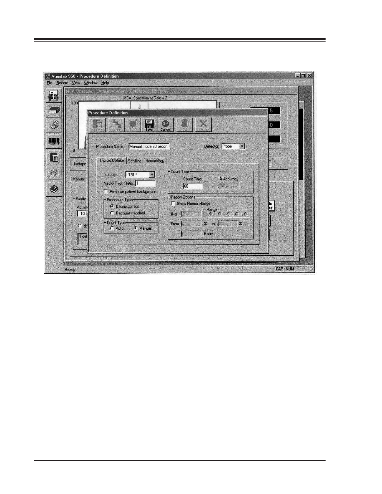
1. INTRODUCTION

Figure 4-1. The Procedure Definition Screen.

THYROID UPTAKE 4-2

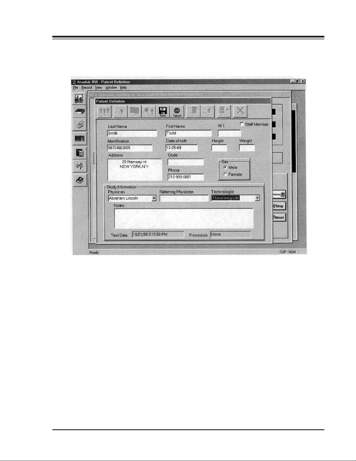
1. INTRODUCTION

Figure 4-2. The Patient Definition Screen.

4-3 THYROID UPTAKE

1. INTRODUCTION

The Patient Definition Screen

(See Figure 4-2.)

On this page, the user can add a new patient, edit existing patient information or select an existing patient
to study. All pertinent information regarding the patient is displayed on this page. Fields are provided for
the Patient Name, Identification Number, Address, Phone Number, Height, Weight, Sex, Date of Birth.
The Study window, at the bottom of the screen, provides fields for Physician, Referring Physician,
Technologist, Notes, Test Date and Procedure.

To Select an Existing Patient

1. To select a patient that has already been entered into the system, click on the <Patient Definition>
icon in the primary tool bar. The Patient Definition screen should now be displayed.

2. Click on <Open> in the screen tool bar. The Patient List should now be displayed.

3. Double-Click on the desired patient to select that patient. The Patient Definition screen should now
be displayed with the new patient selected.

4. Click on <Close> to return to the Operation screen. The selected patient should now appear at the
top of the screen.

To Edit an Existing Patient

1. To edit an existing patient, click on <Patient Definition> in the primary tool bar. The Patient
Definition screen should now be displayed.

2. Click on <Edit> in the screen tool bar. The Patient List should now be displayed.

3. Double-Click on the desired patient to select that patient. The Patient Definition screen should now
be displayed with the patient to edit selected.

4. Make the necessary edits by highlighting each parameter to edit, then keying in the new
information.

5. Click on <Save> to save the edits.

6. Click on <Close> to return to the Operation screen. The edited patient should now appear at the top
of the screen.

To Add a New Patient To the Patient List

1. To Add a new patient to the Patient List, <Patient Definition> in the primary tool bar. The Patient
Definition screen should now be displayed.

2. Click on <Add> in the screen tool bar. The fields on the Patient Definition screen should now be
highlighted.

3. Enter all pertinent information on the Patient Definition screen and in the Study Information
window at the bottom of the screen.

4. Click on <Save> in the screen tool bar to save the new patient. The System will prompt you to add a
procedure to the patient file.

5. Click on <Okay> to access the Procedure Selection screen. Click on <Expand All> or <+> to show
the patient information. Highlight the desired procedure and click on <Select>. The system now
returns to the Operation screen.

THYROID UPTAKE 4-4

CONTENTS

NOTE: If there is an existing patient and at some future time another uptake study with a new dose will be
administered, you would go to the Patient Definition screen, select the desired patient, and either select an
existing study or click on <Add Test To Selected Patient>. This allows the addition of a new test to the selected
patient. This can be another uptake study with a new dose, a Schillings test or some other function.

DETERMINING AUTOMATIC COUNT TIME

If automatic counting is selected in the Procedure Definition, the time period for each measurement
becomes a variable. Measurement will continue until a predetermined accuracy is reached as determined
by random counting statistics.

For automatic measurements, statistical uncertainty is user defined (i.e., 1%, 3%, 5%, etc.). The time is
based on the radioactive level of activity being measured, the background level, the type of measurement
being made, and the user selected percent accuracy. The system performs an internal check to ensure the
count was accomplished with an acceptable degree of certainty (i.e., appropriate counting rate, proper
spectrum, etc.). The level of accuracy is also set from the Preferences screen.

With automatic counting selected, each count time for a thyroid uptake measurement is automatically
determined, using counting statistics, by imposing an overall accuracy requirement on the uptake result.
There are four count times which comprise an uptake measurement: Standard, Lab Background, Thyroid
and Patient Background. Each count resulting from a lapsed count time has a statistical uncertainty which
is related to the count. When these four independent counts are combined to yield the uptake value, the
uncertainties must also be combined to yield the total uncertainty of the uptake. This total uncertainty is
preset by the user, in Setup Preferences, when the instrument is installed.

At the start of an uptake procedure, the total uncertainty is partitioned between the four count times in a
rational way which minimizes the count times for all four counts and thereby minimizes the amount of
time the patient must remain immobile. Because the count rate is high, the Standard count time is usually
short (~6 seconds). Time for the Lab Background is determined from the first few seconds of Lab
Background counting. If the count rate is very low, the count time will be short because the net error of
(Std.-Bkgd.) contains only a term proportional to (Bkgd. rate/Std. Rate).

Thyroid count time is also determined during the first few seconds of Thyroid counting. It is calculated
from the approximate Thyroid rate and the Standard count rate in such a way that the Thyroid
measurement uncertainty will be only a fraction of the total target uncertainty. Finally, the Patient
Background is determined during its first few seconds of counting with the requirement of the total
uncertainty satisfying the accuracy goals.

Examples

The following academic numerical examples should provide some idea of the four required measurement
times in actual practice. Each example assumes a user-selected counting accuracy requirement of 98%.
This means that there is a 2% allowed counting error at the 90% confidence level. If you repeat each of the
four measurements and calculate the uptake, nine out of ten results will fall within 2% of the first
measurement.

NOTE: You must select the accuracy requirement in the Uptake Procedure Setup loop. The factory setting is 95%,
if you want 98% as illustrated in this example, you must select it. The counting times get longer with higher
accuracy requirements.

NOTE: The “2%” uncertainty is only with respect to detector counting. If a measurement is “repeated” with
repositioning of the standard or patient, there will be additional geometry setup errors which will add to the
counting errors.

NOTE: The % uncertainty is not an uptake %, but a percentage of the uptake. For example, if the uncertainty is 2%
and the uptake is 50%, then the uncertainty is 2% of 50%, or ±1%, and the uptake range could be 49% to 51%. If
the uptake was 10%, the uptake could be 9.8% to 10.2% (2% of 10% is 0.2%).

4-5 THYROID UPTAKE

CONTENTS

Maximum Count Time

All of the following examples had a 60 sec maximum count time set in the Uptake SETUP loop. The first
example did not require longer than 60 seconds on each measurement to satisfy the 98% accuracy
requirement. The next two examples did require a longer than 60 seconds on each measurement to satisfy
the 98% accuracy requirement. The next two examples did require a longer than 60 seconds on some of
the measurements but the actual time was limited to 60 seconds automatically. The uncertainty resulting
from such a shortened time is stated with the example.

Minimum Count Time

The minimum count time for any count in the uptake mode is 10 seconds. This is illustrated in all three
examples during the lab background count.

EXAMPLE 1: I-123, 6 HOUR UPTAKE, 98%, 60 SEC MAX COUNT TIME

cpm

Measured Standard

Measured Lab Bkgnd

Decayed Standard

Measured Thyroid

Measured Pat. Bkgnd

Comment

The automatic time selection controlled the counting since all times were less than the maximum set
count time of 60 sec. The patient was required to remain in a counting position for only 29 seconds for the
thyroid and 12 seconds for the background count. This is very beneficial for hyperthyroid and elderly
patients. Plus the auto-count time mode takes less time to set up. The Uptake of 25.5% has a 2%
uncertainty meaning it could be 25.1% to 26.1%.

NOTE: In this example, and the following two, the “pill” was counted at the time of administration (Measured
Standard) and the count rate was decayed to the time of the thyroid count (value in parenthesis).

EXAMPLE 2: I-123, 6 HOUR UPTAKE, 98%, 60 SEC MAX COUNT TIME

538,920

64

(393468)

108,060

7,500

Uptake = 25.5% 2% (25.1% to 26.1%)

+

-

Actual Count

Time

53 sec

10 sec

29 sec

12 sec

Computed Auto

Time

53 sec

2.2 sec

29 sec

12 sec

cpm

Measured Standard

Measured Lab Bkgnd

Decayed Standard

Measured Thyroid

Measured Pat. Bkgnd

THYROID UPTAKE 4-6

538,920

64

(393468)

36,000

12,000

Uptake = 6.1% 2.3% (5.96% to 6.24%)

+

-

Actual Count

Time

53 sec

10 sec

60 sec

60 sec

Computed Auto

Time

53 sec

2.2 sec

119 sec

81 sec

1. INTRODUCTION

Comment

The uptake was about one fourth the values as in example 1 in order to illustrate the change in counting
time required for uptake and patient background. If the maximum set count time was 120 seconds, then
the actual counting times for the thyroid and patient background would have been 119 and 81 seconds
respectively. The standard and lab count rates were kept the same for demonstration purposes.

Note: Even though the actual count times were lower than the required time for a 2% uncertainty, the
times used (thyroid time almost 1/2 of the computed value) resulted in only an increase of 0.3%
uncertainty. This is certainly not significant, particularly in view of the low uptake where count times will
tend to be longer because of the lower count rates.

EXAMPLE 3: I-123, 6 HOUR UPTAKE, 98%, 60 SEC MAX COUNT TIME

cpm

Measured Standard

Measured Lab Bkgnd

Decayed Standard

Measured Thyroid

Measured Pat. Bkgnd

120,000

300

(87612)

12,000

3,600

Uptake = 9.6% 2.8% (9.33% to 9.87%)

Comment

In this example, we see much lower rates in the standard and thyroid counts. However, the standard
count time only increased by 2 seconds. The reason for this is twofold. First, the equations for time
computation derived from counting statistics are nonlinear. Second, pulse height analysis at the higher
counting rates takes a longer period of time.

The increase in lab background time is due to the increase in lab counting rate and how the standard and
lab rates are treated in the analysis. The lab is subtracted from the standard. Any error in the lab is carried
forward into the overall error, but the impact depends upon the relative counting rates. If the standard is
10,000 times higher than the lab, then a 50% uncertainty in the lab will only contribute a very small error
to the difference. As the lab rate increases with respect to the standard, its error contribution will also
increase which will require a more precise measurement of the lab.

Actual Count

+

-

Time

55 sec

10 sec

60 sec

60 sec

Computed Auto

Time

55 sec

5.3 sec

156 sec

90 sec

The thyroid count time increased significantly but the actual count time again was only 60 seconds
because of the maximum time set. Note the increase in the uptake uncertainty went to 2.8%, due to the
reduction of actual counting times from time values which were required for the thyroid and patient
background measurements.

PERFORMING A THYROID UPTAKE

(See Figure 4-3.)

To Perform A Thyroid Uptake

1. Click on <Patient Definition> in the primary tool bar. Select an existing patient, edit an existing
patient, or create a new patient to test. For existing patients, proceed to step 3. If you have just
created a new patient, click on <Close>.

NOTE: You can access the Patient Definition screen from any other screen by simply clicking on <Patient

4-7 THYROID UPTAKE

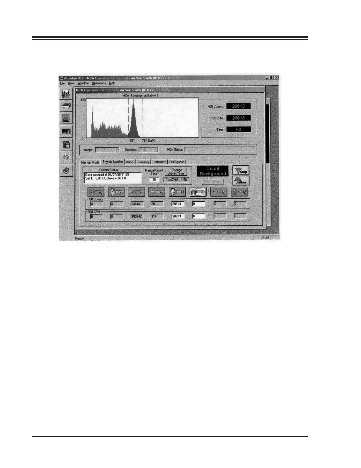
1. INTRODUCTION

Figure 4-3 The Thyroid Uptake Screen.

THYROID UPTAKE 4-8

INTRODUCTION

Definition> in the primary tool bar. After selecting a patient, you can then access any mode of operation with
the new patient selected.

2. For existing patients, click on the patient name to reveal the studies. Double-click on the desired
study to return to the Thyroid Uptake screen with the patient and study selected.

3. The Thyroid Uptake screen should now be displayed. At the top of the screen should be the
currently selected patient and I.D. number. Confirm that this is the correct patient and correct I.D.
number for the patient to be tested.

4. Position the capsule(s) in the thyroid phantom and set up the collimator for use. Set the distance on
your distance bar and move the collimator down to this distance. The capsule count distance and the
thyroid count distance must be the same for all counts.

5. If testing an existing patient, proceed to step 9. For a new patient, click on the <Capsule> icon (third
from left, above the time titled ROI Counts) to begin counting. The message "Counting Dose"
appears on the right of the screen. The current system status is displayed on the left side of the
screen in the "Current Status" box.

NOTE: Once counting begins, the counts are shown in the spectrum at the top of the screen. ROI counts, ROI
cpm and elapsed time are indicated in the upper right. When the system finishes counting, it will stop and do a
final download for the best spectrum. If you desire to do a spectrum analysis, click on the <Spectrum> icon in
the primary tool bar.

6. Remove the capsule from the neck phantom and position the probe to measure lab background.
Click on the <Lab Background> icon (fourth from left, above ROI counts) to begin the lab
background count. In auto count time, the system will calculate the count rate and adjust the
counting time automatically. For manual counting, the system counts for the time selected.

7. When the lab background count is complete, the system prompts the user to save the dose count
results. Click on <Yes> to save the results.

NOTE: If you are not satisfied with the results for dose or lab background, click <No>. You can then
reposition for the appropriate count and click the desired icon to recount for that function.

8. When you are finished counting the dose and lab background, save the results.

9. Give the dose to the patient.

NOTE: If you do not immediately give the dose to the patient, you can correct the administration time by
clicking on <Change Administration Time>.

10. Tell the patient when to return.

11. When the patient returns, go to the Patient Window and select the patient and study. The system
will display the thyroid counting page. If you are using decay correction <Count Thyroid> will be
highlighted.

12. Position the probe over the patient's neck.

13. Click on the <Thyroid Count> icon (fifth from left, above ROI counts) to begin the thyroid count.

14. Once the thyroid count is complete, position the probe over the patient's thigh. Click on <Patient
Background> (sixth from left, above ROI counts) to begin the patient background count.

15. When patient background counting is complete, the system displays a message that "A Thyroid

4-9 THYROID UPTAKE

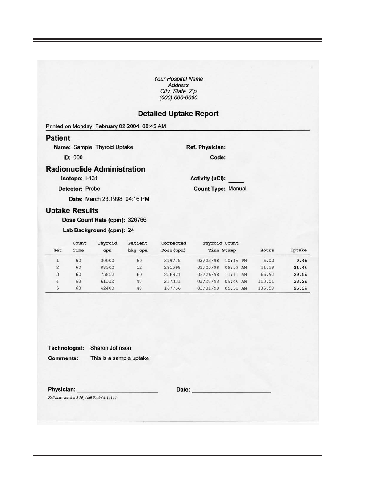
1. INTRODUCTION

Figure 4-4. A Thyroid Uptake Report.

THYROID UPTAKE 4-10

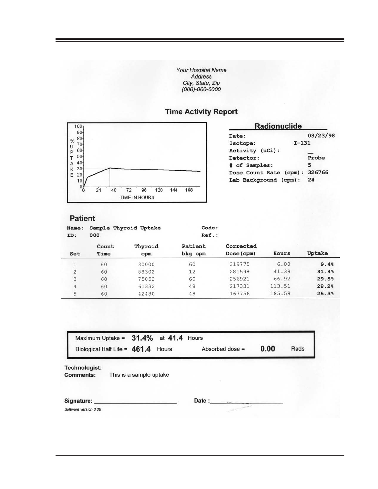
1. INTRODUCTION

Figure 4-5. A Time Activity Report.

4-11 THYROID UPTAKE

CONTENTS

Uptake Is Complete" and prompts you to save the results. If you click <Yes> the results are stored and
cannot be changed. If you click <No> and do not save the results, the system allows you to recount the
thyroid and patient background. It is recommended that the results be saved if they are satisfactory.

After saving the thyroid uptake results, the system returns to the MCA Operation screen. You can
now use the system for other operations if desired. If you come back to this patient at a later time,
follow steps 1-3 and then go to step 11.

NOTE: Click on <Stop> at anytime to stop counting and use the counts up to that point for results. Click on
<Abort> to cancel the current counting operation without using the current count. You can then go in and
manually change the numbers if you have selected this option in your procedure definition.

16. If you are using a procedure to recount a standard, the system will highlight the button to count the
standard.

17. Place the standard in the neck phantom.

18. Click <Count Standard>.

19. Remove the standard from the phantom and store it away.

20. Count the empty phantom to obtain the current lab background count.

21. The system now displays a prompt to save results. Click <Yes> to save the results with the number.
Click <No> to redo any count.

22. When satisfied, save the results.

After saving the thyroid uptake results, the system returns to the MCA Operation screen. You can now
use the system for other operations if desired. If you come back to this patient at a later time, follow steps
1-3 and then go to step 11.

Printing A Thyroid Uptake Report

(See Figure 4-4.)

1. After saving a Thyroid Uptake as described above, click on the <Report> icon in the primary tool
bar. The Report Generation screen should be displayed.

2. Click on the desired parameters, including Thyroid Uptake test, then key in the Technologist name
(or select the desired name from the pull-down technologist list). Key in dose activity and any
comments to be printed on the report.

3. Click on <Preview> if you want to preview how the report will look when it is printed.

4. Click on <Print> to print the report.

5. Click on <Close> to return to the Thyroid Uptake screen.

Printing A Time Activity Uptake Report

(See Figure 4-5.)

The Time Activity Curve plots a decay curve showing the decay of the isotope in the thyroid. Several data
sets must be counted before printing this report. The report should be printed when half the original rate
remains in the thyroid.

THYROID UPTAKE 4-12

1. INTRODUCTION

1. After saving a Thyroid Uptake as described above, click on the <Report> icon in the primary tool
bar. The Report Generation screen should be displayed.

2. Click on the desired parameters, including Time/Activity for Thyroid Uptake, then key in the
Technologist name, dose activity and any comments to be printed on the report.

3. Click on <Preview> if you want to preview how the report will look when it is printed.

4. Click on <Print> to print the report.

5. Click on <Close> to return to the Thyroid Uptake screen.

NOTE: Results can be listed in rads or in grey units of measure. See Section 2, “System Set-Up.”

6. Click on <Print> to print the report.

7. Click on <Close> to return to the Manual Mode screen.

4-13 THYROID UPTAKE

5. MANUAL MODE

The MCA Manual mode is used as a rate counter that functions in either a Preset Time, Preset Count or
Continuous Counting mode. You can press Spectrum for any count that you take in this mode and create
reports from the data obtained. The standard ROI is determined by the isotope that you are counting and
the spectrum analysis page will allow you to create multiple ROI’s or change the ROI displayed.

To Count In Manual Mode

(See Figures 5-1 and 5-2)

1. From the Operation screen, click on <Manual Mode>. The Manual Mode screen should now be
displayed.

2. Select the desired <Isotope> and <Detector>.

3. Toggle on <Preset Time>, <Preset ROI Counts> or <Continuous Counting> and enter the desired
count time or number of counts.

• Preset time count: When counting by preset time, the system counts for the time entered.

• Preset ROI count: The system counts to just beyond the number of ROI counts entered.

• Continuous counting: The system will count until <Stop> is pressed.

4. Click on <Start>. The system displays a message on the right side of the screen stating that a test is in
progress. The spectrum is displayed at the top of the screen, along with the associated time, counts
and cpm.

NOTE: Click on <Stop> at anytime to stop counting and use the counts up to that point for results. Click on
<Abort> to cancel the current counting operation without using the current count. The system will return to
the Manual Mode screen.

5. Once the count is completed, the message "Test Completed" is displayed. The results now appear in
the Test Results window. You may now count again in manual mode to build a report with multiple
counts, or exit to another mode.

NOTE: Click on <Clear All> to clear all counts stored in the Test Results window. To remove a particular line
from the window, highlight the line to be removed and click on <Remove>.

To Print a Manual Report

1. Click on the <Report> icon in the primary tool bar. The Report Generation screen should be
displayed.

2. Click on the desired parameters, including Administration or Test. Key in the Technologist name
and any comments to be printed on the report.

3. Click on <Preview> if you want to preview how the report will look when it is printed.

4. Click on <Print> to print the report.

5. Click on <Close> to return to the Manual Mode screen.

NOTE: The Manual Report allows for listing of multiple isotopes. This allows the operator to perform any
variation of the test or procedures deem desirable.

Spectrum Analysis

After any count is taken, the Spectrum Analysis option can be used to analyze counts in the spectrum and
print a Spectrum Analysis Report if desired.

5-1 MANUAL MODE

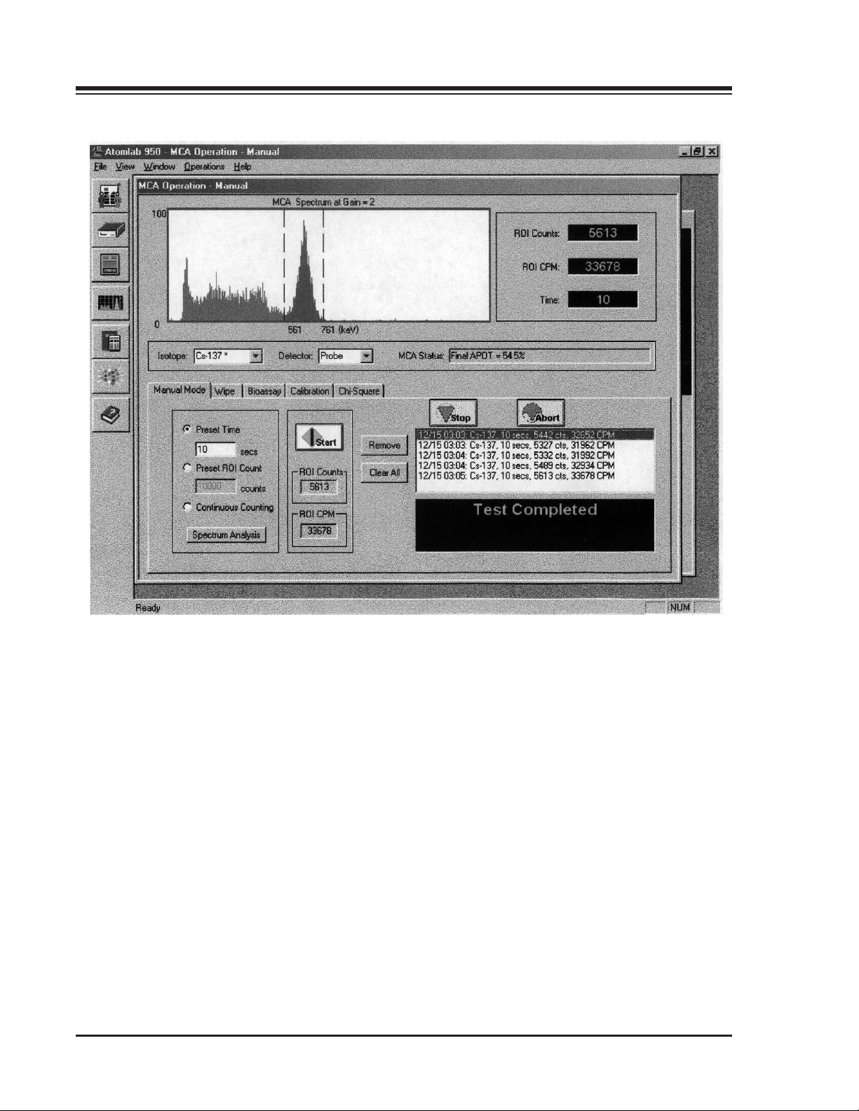
1. INTRODUCTION

Figure 5-1. The Manual Mode Screen.

MANUAL MODE 5-2

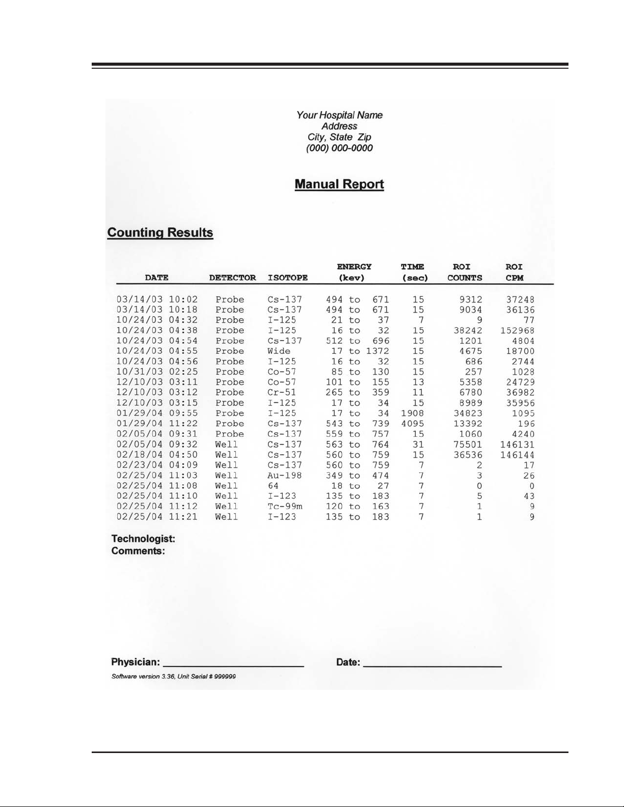
1. INTRODUCTION

Figure 5-2. A Manual Mode Report.

5-3 MANUAL MODE

6. WIPE TEST

(See Figures 6-1 - 6-5.)

The Wipe Test is used to determine the DPM of swipes taken in the designated areas of a department
using the optional well counter Model #187-246. A total of 10 swipes may be identified and counted for
each area. When wipe counting is completed, a report of the Wipe Test results can be printed out with
each test identified by the area and wipe with results shown. The screen displays all wipes and stores the
results for each wipe until that wipe is recounted.

NOTE: In Wipe Test and Bioassay mode, the activity shown is NET activity. This means that the background count
is subtracted from the count before the activity is calculated. For all other modes, counts shown are the actual counts
detected and are not netted for background.

Define Wipe Areas

The Define Wipe Areas feature is used to define new areas or change information about existing areas. At
this screen, you can define individual wipe areas in the same manner as used for selecting, adding,
editing or deleting patients and isotopes.

NOTE: You must use the Isotope Editing screen to make isotopes available for use in Wipe Testing, and the Isotope
Efficiencies screen to enter the Detector Efficiency for each isotope. Refer to chapter 3 for details.

To Edit an Existing Wipe Area

1. To edit an existing Wipe Area, at the Operation screen click on <Wipe>. The Wipe Counting screen
should now be displayed.

2. Click on the <Define Wipe Area> icon at the bottom of the screen. The Wipe Area Setup screen
should now be displayed.

3. If the currently selected wipe area is the one you want to edit, proceed to step 5. To select another
wipe area to edit, click on <Open> in the screen tool bar. The Wipe Area Selection List should now
be displayed.

4. Double-Click on the desired wipe area. The selected wipe area should now be displayed on the Wipe
Area Setup screen.

5. Click on <Edit> in the screen tool bar and then make the desired changes.

6. Click on <Save> to save the changes.

NOTE: If you click <Cancel> the changes made will be discarded.

7. Click on <Close> to return to the Wipe Counting screen. The edited wipe area should now be
displayed in the Area Name box.

To Add A New Wipe Area

1. To add a new Wipe Area, at the Operation screen click on <Wipe>. The Wipe Counting screen
should now be displayed.

2. Click on the <Define Wipe Area> icon at the bottom of the screen. The Wipe Area Setup screen
should now be displayed.

3. Click on <Add> in the screen tool bar. The fields on the Wipe Area Setup screen should now be
highlighted.

4. Enter the new wipe area name and up to ten wipe locations in this area (i.e., Camera Room or Hot
Room for area names, counter, table, etc. for locations.)

5. Select the area type: restricted, unrestricted or sealed source.

NOTE: If you select a sealed source area only one isotope is allowed. For restricted and unrestricted areas,
multiple isotopes can be used.

6-1 WIPE TEST

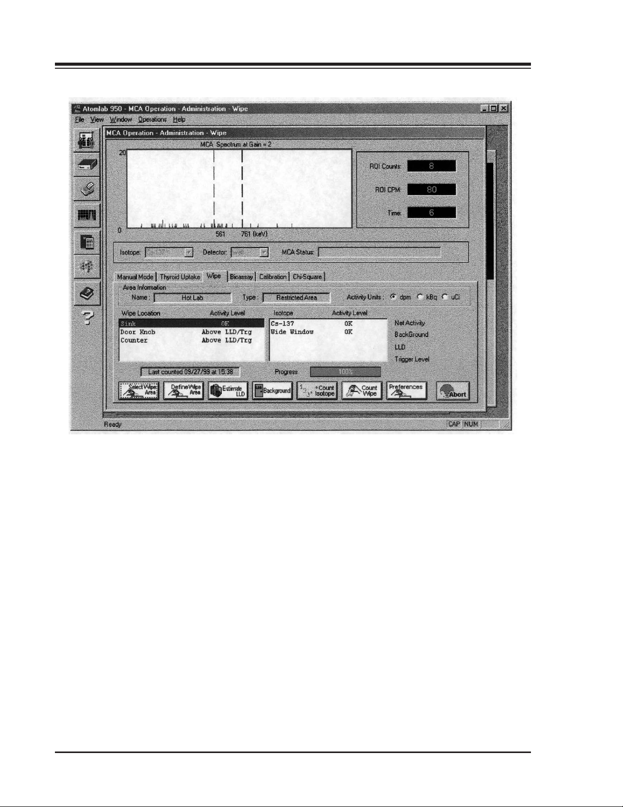
1. INTRODUCTION

Figure 6-1. The Wipe Counting Screen.

WIPE TEST 6-2

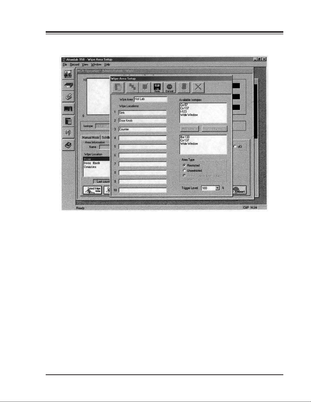
CONTENTS

Figure 6-2. The Wipe Area Setup Screen.

6-3 WIPE TEST

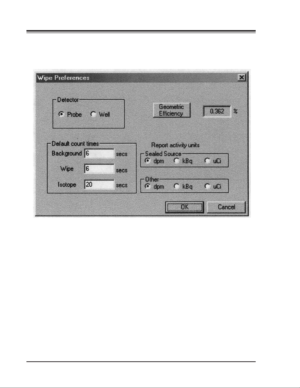
CONTENTS

Figure 6-3. The Wipe Preferences Window.

WIPE TEST 6-4

1. INTRODUCTION

6. In the Available Isotopes list, highlight an isotope and click on <Add to Area>. The isotope name
will now be displayed in the lower box. If desired, highlight additional isotopes on the Isotope List
and add them to the lower box. To remove an isotope from the box, highlight the isotope in the
lower box and click on <Remove From Area>.

7. Set the trigger level.

NOTE: The trigger level is factory set to 100%. The 100% refers to the NRC trigger levels for different
isotopes. If you want tighter control, lower the trigger level. Use the scroll to the right of the trigger level to
select a different percentage.

8. Click on <Save> in the screen tool bar to save the new wipe area. The new wipe area should now be
shown on the Wipe Area Setup screen.

9. Click on <Close> to return to the Wipe Counting screen with the new area displayed in the Area
Name box.

To Delete A Wipe Area

1. To delete an existing Wipe Area, at the Operation screen click on <Wipe>. The Wipe Counting
screen should now be displayed.

2. Click on the <Define Wipe Area> icon at the bottom of the screen. The Wipe Area Setup screen
should now be displayed.

3. If the currently selected wipe area is the one you want to delete, proceed to step 5. To select another
wipe area to delete, click on <Open> in the screen tool bar. The Wipe Area Selection List should now
be displayed.

4. Double-Click on the desired wipe area. The selected wipe area should now be displayed on the Wipe
Area Setup screen.

5. Click on <Delete> in the screen tool bar.

6. Click on <Yes> to delete.

7. Click on <Close> to return to the Wipe Counting screen. The next wipe area on the Wipe Area
Selection List should now be displayed in the Area Name box.

Select Wipe

To Select an Existing Wipe Area

1. To select a wipe area that has already been entered into the system, at the Operation screen click on
<Wipe>. The Wipe Counting screen should now be displayed.

2. Click on the <Select Wipe> icon at the bottom of the screen. The Wipe Area Selection list should now
be displayed.

6-5 WIPE TEST

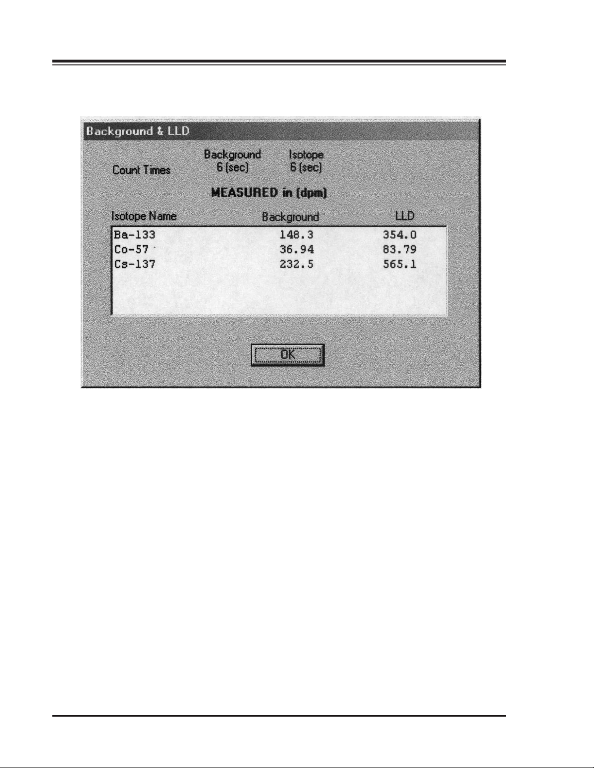
1. INTRODUCTION

Figure 6-4. The Background LLD Screen.

WIPE TEST 6-6

CONTENTS

4. Double-Click on the desired wipe area to select the wipe, or highlight the wipe and click on <Select>.
The system returns to the Wipe Counting screen with the selected wipe now displayed in the Wipe
Area Name box.

NOTE: If you click <Close> on the Wipe Area Selection List, the system returns to the Wipe Counting screen
with the original wipe still selected.

7. Click on <Close> to return to the Wipe Counting screen. The edited wipe area should now
be displayed in the Area Name box.

Wipe Preferences

The Wipe Preferences screen allows the user to specify the detector, default count times for background,
wipe and isotope counting, and the geometric efficiency for the detectors. It also allows selection of the
report activity units (in dpm, becquerels or microcuries) that will be used for sealed sources or other
wipes.

1. From the Operation screen, click on <Wipe>. The Wipe Counting screen should now be displayed.

2. Click on <Preferences> at the bottom of the screen. The Wipe Preferences screen should now be
displayed.

3. Select the appropriate detector.

4. Enter default count times for background, wipe and isotope counting.

5. Select the desired report activity units, DPM, kBq or µCi.

6. If you have not already done so, set the Geometric Efficiency as explained in the Administration
section of this manual.

7. Once all parameters have been set, click on <Ok> to return to the Wipe Counting screen.

BACKGROUND

Before performing a wipe test, the system must perform a daily background count. The system requires
that you count background a minimum of one time per day. If the background changes dramatically in a
facility during the day, it is recommended to recount your background at the appropriate intervals.

NOTE: A 60-second background count is recommended. This means that each gain will be counted for 60 seconds.

1. From the Operation screen, click on <Wipe>. The Wipe Counting screen should now be displayed.

NOTE: If desired, you can at this point click on the <Estimate LLD> icon at the bottom of the screen. This will
provide a quick count and estimate of the Lower Limit of Detection (LLD) using the actual counting
parameters. By lengthening count times the system will have a better LLD.

2. Click on <Background> at the bottom of the Wipe Counting screen. The Background count will
begin automatically. The system will count the gains for all isotopes that have been turned on for
wipe testing. If multiple isotopes use the same gain, the system will only count the gain once, using
the appropriate regions of interest to calculate the dpms associated with this region for the selected
gain. As the system counts, a slidebar at the left of the screen shows the percentage completed. Wipe
locations are listed to the right of the slide bar with any results of previous wipes.

6-7 WIPE TEST

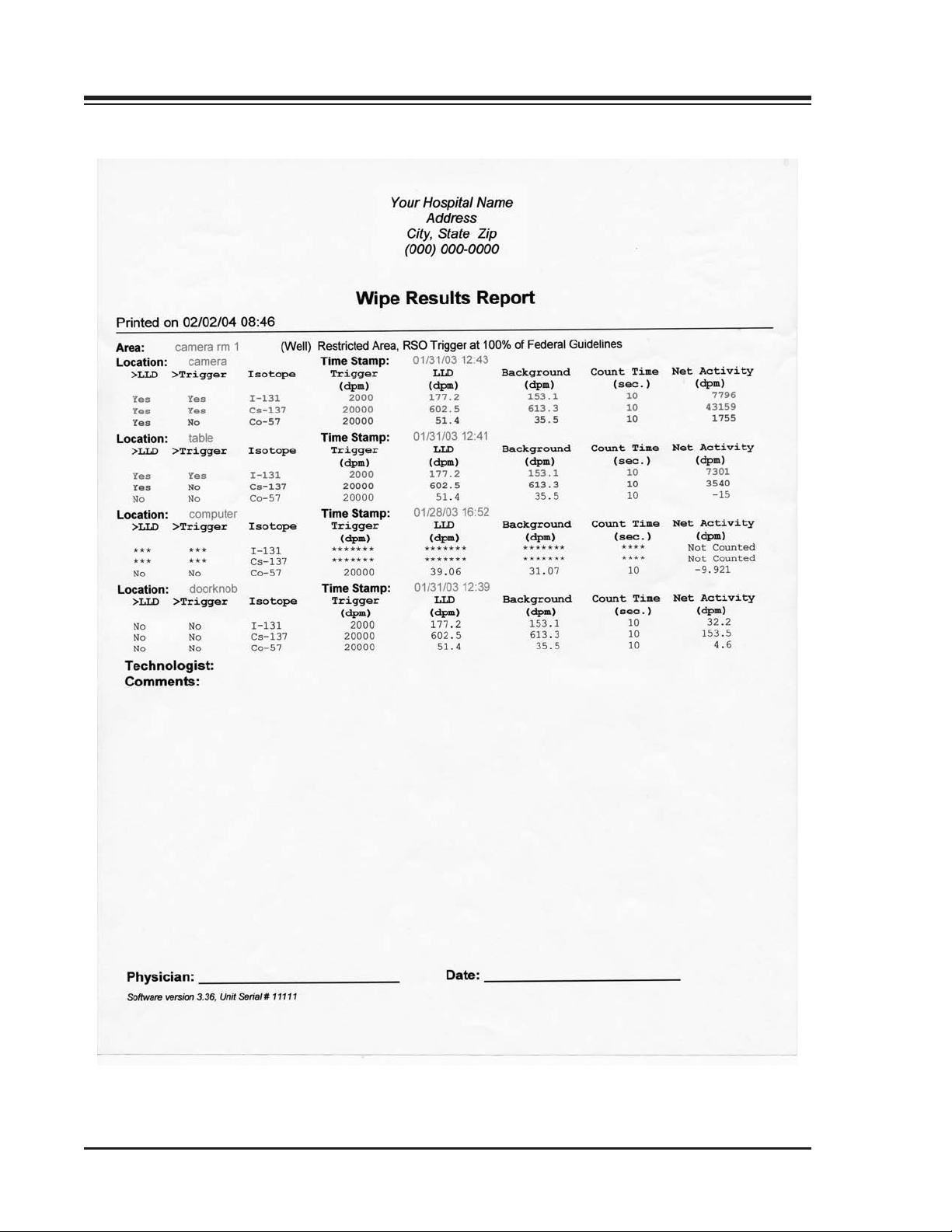
1. INTRODUCTION

Figure 6-5. The Wipe Results Report.

WIPE TEST 6-8

1. INTRODUCTION

3. Once the background count is completed, the Background and LLD screen displays the results. Click
on <OK> to accept the results and return to the Wipe Counting screen. If the results are not
acceptable, click on <Background> again and perform another background.

NOTE: <Estimate LLD> displays the same style results screen except it notes that the LLD is an estimate, not
measured. The estimate LLD counts for ten seconds each.

PERFORMING A WIPE TEST

1. From the Operation screen, click on <Wipe>. The Wipe Counting screen should now be displayed.

2. Click on <Select Wipe Areas> at the bottom of the screen. The Wipe Area Selection list should now
be displayed.

3. Double-click on the desired wipe area to select it and return to the Wipe Counting screen.

NOTE: If you have not yet performed a background count on this date, you must do so before proceeding with
the wipe test.

4. Click on the wipe location to be counted. If this wipe has been counted previously the system
displays the last count date and time.

5. Click on <Count Wipe> to perform the wipe test. The system now counts for only the isotope listed
in this area.

6. Once the wipe test is completed, the results of that wipe location are stored by date and time until
that particular wipe is recounted. The screen displays the results, in cpm, next to each isotope in the
isotope display window. The last isotope spectrum counted will be displayed at the top of the screen
with the ROI cpm shown to the right of the spectrum on the lower part of the screen. To the right of
the Isotope Results are listed the net activity, background, lower limit of detection, trigger level and
activities. These are shown in either cpm, bq, or microcuries.

To look at the net activity of any isotope, highlight the isotope desired in the Isotope Results window.

NOTE: The <Count Isotope> option is available for use only if an isotope has been highlighted in the Isotope Results
window.

If you click on <Count Isotope>, the system will count, for the time frame set under Preferences, only the
highlighted isotope. This allows the user to count for a longer period of time, ensuring better accuracy for
isotopes with high counts.

SPECTRUM ANALYSIS

To perform a detailed spectrum analysis, you must count an isotope using the <Count Isotope> icon for a
specific wipe. The rest of spectrum analysis functions the same way as described previously in this
manual.

6-9 WIPE TEST

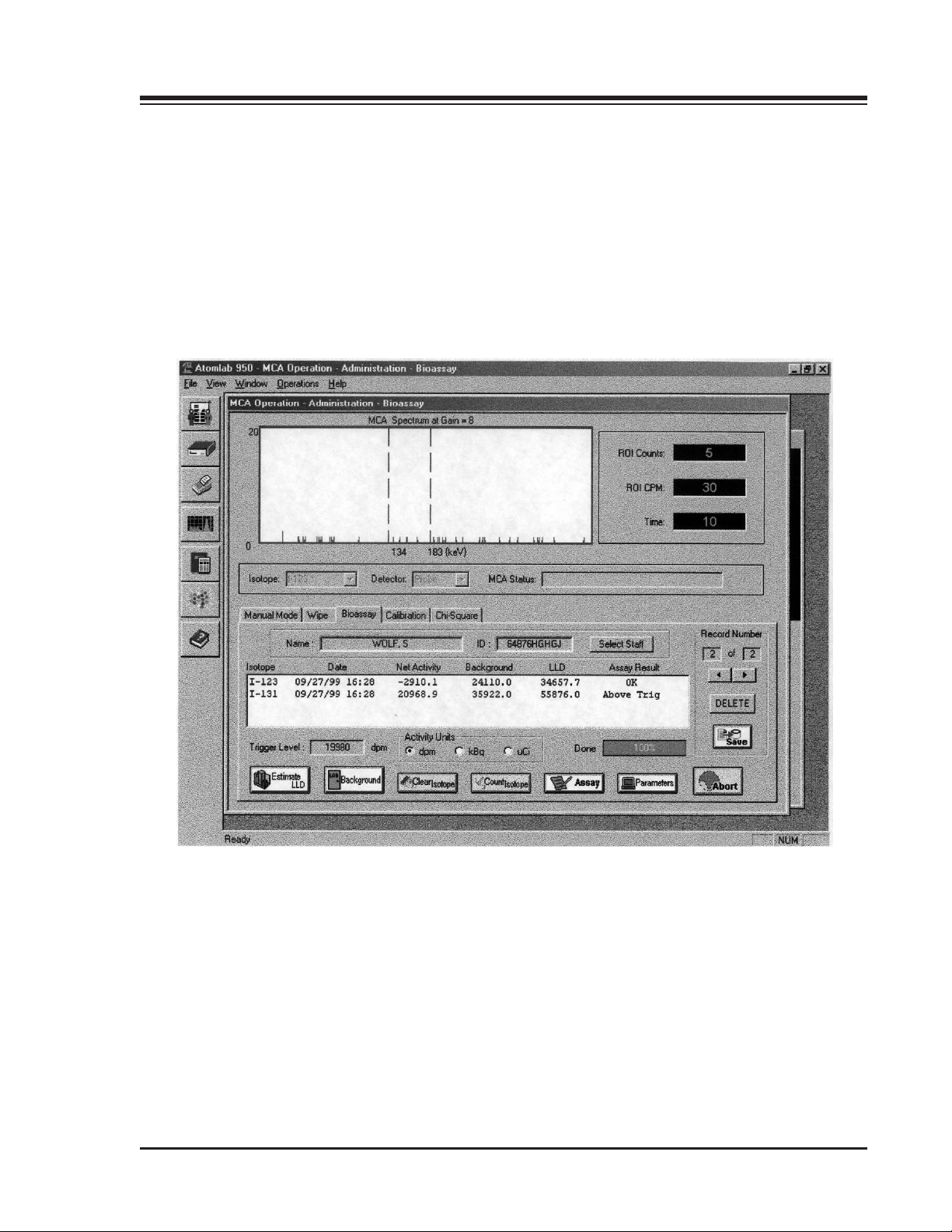
7. BIOASSAY

This mode is used to verify any Iodine 131, 123 or 125 concentration for staff or a patient who have direct
contact with radioactive iodine or radioactive patients. A record may then be printed out for an
individual, as a Bioassay History, or as a Bioassay Employee Summary.

NOTE: In Bioassay and Wipe Test mode, the activity shown is NET activity. This means that the background count
is subtracted from the count before the activity is calculated. For all other modes, counts shown are the actual counts
detected and are not netted for background.

NOTE: You must use the Isotope Editing screen to make isotopes available for Bioassay use, and the Isotope
Efficiencies screen to enter the Detector Efficiency for each isotope. Refer to chapter 3 for details.

7-1. The Bioassay Screen.

7-1 BIOASSAY

CONTENTS

To Perform A Bioassay

1. Click on <Patient Definition> in the primary tool bar. Select an existing patient, edit an existing
patient, or create a new patient to test. Click on <Close> to return to the Operation screen.

2. Click on <Bioassay>. The Bioassay screen should now be displayed. The selected patient should be
displayed in the Select Name box along with the proper patient I.D. number, a listing showing the
number of bioassays for this person, and the current bioassay number displayed on the screen.
Multiple bioassays can be stored for each patient. Below this is shown the isotope(s), the date
counted, net activity, background, lower limit of detection, and assay results. Activity units and
Trigger Level are displayed at the bottom of the screen.

3. Click on <Select Staff>. The Staff List should now be displayed. This list includes staff members
only. Staff members cannot be counted for any test other than Bioassay. Select the patient by clicking
on the staff member and return to the Bioassay screen.

NOTE: Staff members are entered in the <Patient Definition> window by clicking on the Staff parameter.

4. Click on <Parameters> at the bottom of the Bioassay screen. The Bioassay Preferences screen should
now be displayed. Highlight the isotopes you wish to assay in the Available Isotopes Window. Click
on <Add> to add the selected isotopes to the Isotopes for Assay window (you must add one isotope
at a time.) To remove an isotope from the Isotopes for Assay Window, highlight the desired isotope
and click on <Remove>.

5. Select the Detector and Activity Units.

6. Set the appropriate counting times.

7. Set Geometric Efficiency.

8. Set the Trigger Level.

9. After all parameters are set, click on <OK>. The system returns to the Bioassay screen.

NOTE: If you have not yet performed a background count on this date, you must do so before proceeding with
the bioassay. Click on <Background> to count the background. This will count the gain for all isotopes that
have been turned on for Bioassay. If multiple isotopes use the same gain, the gain will be counted only once.

10. Click on <Assay> at the bottom of the screen. The system will assay the patient for all isotopes
associated with the selected patient.

NOTE: If you click on <Assay> the system will count for the time frame set under Preferences, all the gains
necessary for the isotopes that have been made available for bioassay.

NOTE: The <Count Isotope> option is available for use only if an isotope has been highlighted in the Isotope
Results window. If you click on <Count Isotope>, the system will count, for the time frame set under
Preferences, only the highlighted isotope. This allows the user to count for a longer period of time, ensuring
better accuracy for isotopes with high counts.

11. To print a Bioassay Report, click on the <Report> icon in the primary tool bar. You can then select
from Individual Bioassay Report, Individual Bioassay History Summary, or Employee Bioassay
Summary.

12. If you want to change the contamination trigger level, double-click in the box and enter the new
contamination value.

BIOASSAY 7-2

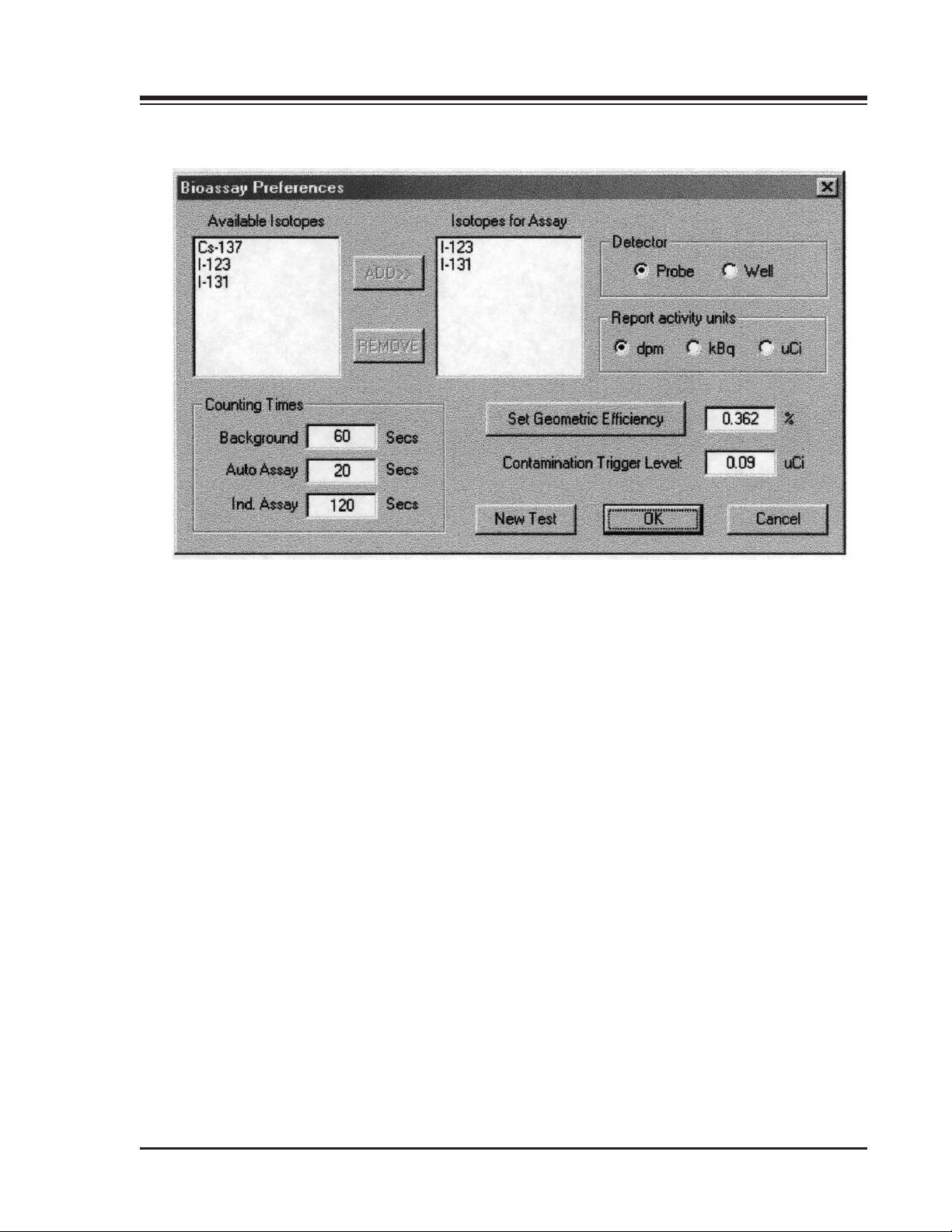
1. INTRODUCTION

Figure 7-2. The Bioassay Preferences Screen.

7-3 BIOASSAY

CONTENTS

NOTE: If you change the trigger level, the new amount is used for all new tests.

13. After assaying a patient or staff member and accepting the count, press <Save> to save the
information..

NOTE: When you wish to perform an additional assay for this patient, click on <Parameters> and then click
on <New Test>.

15. If you click on the arrows under the record number, you can see the record number increase or
decrease and display the appropriate results for each test.

NOTE: In order to count a patient in Bioassay, you must select that patient in the <Patient Definition>
window. Select an existing procedure for the patient, then click on Bioassay to display that patient and any test
data. The Bioassay information is not listed as a test, having been performed in the <Patient Definition>
window. To add a Bioassay record to the patient, click on <Parameters> and then click on <New Test>.

BIOASSAY 7-4

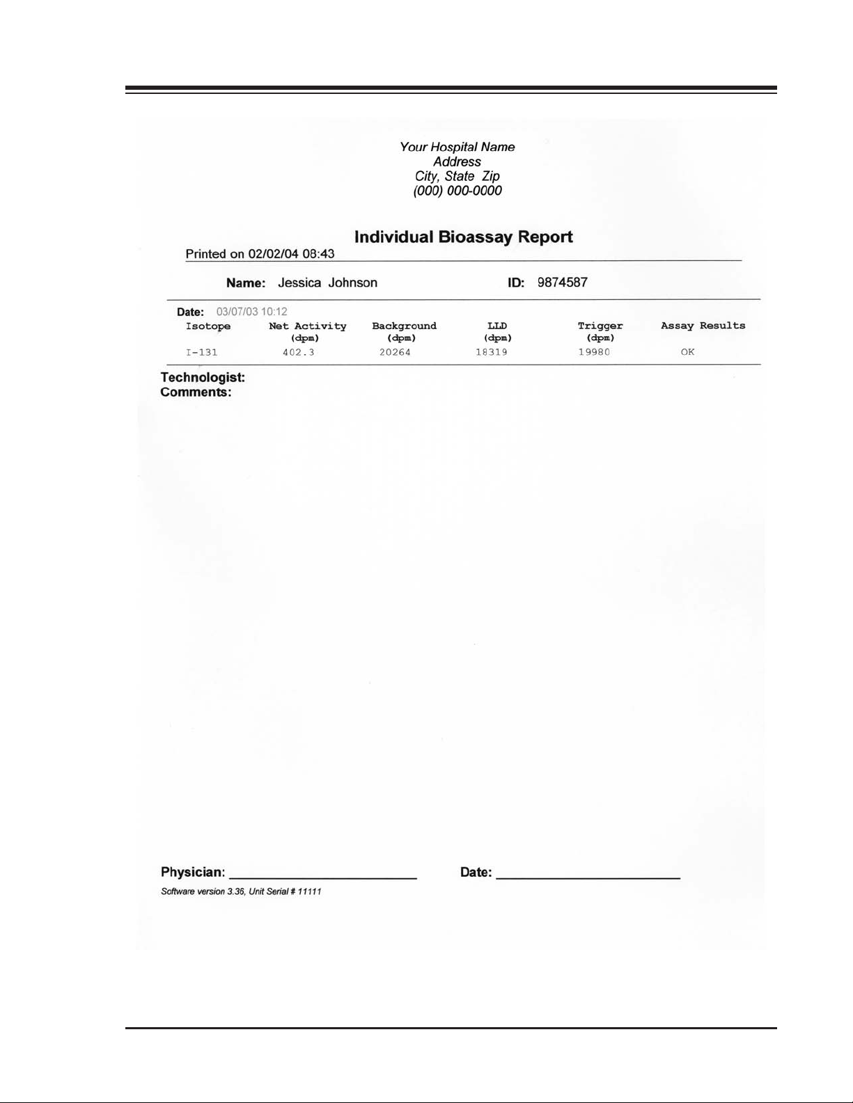
CONTENTS

Figure 7-3. An Individual Bioassay Report.

7-5 BIOASSAY

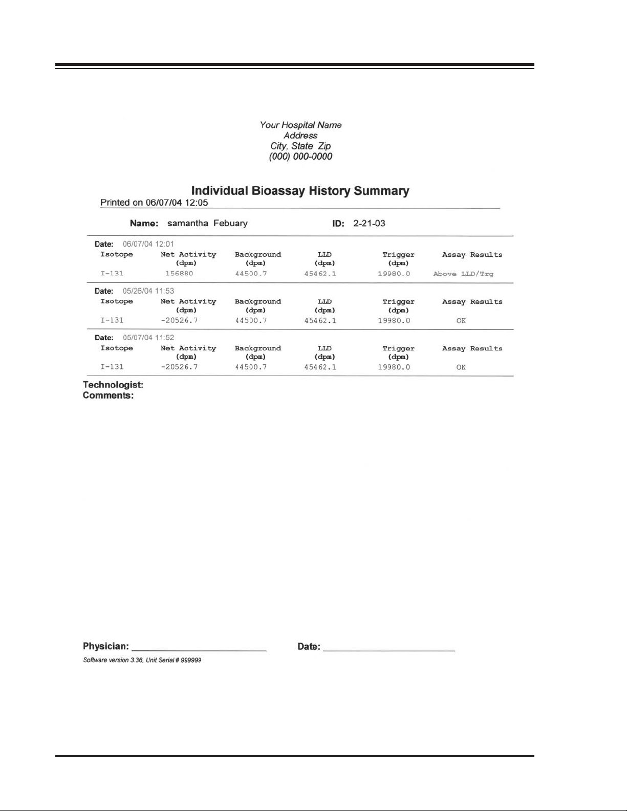
CONTENTS

Figure 7-4. An Employee Bioassay Summary.

BIOASSAY 7-6

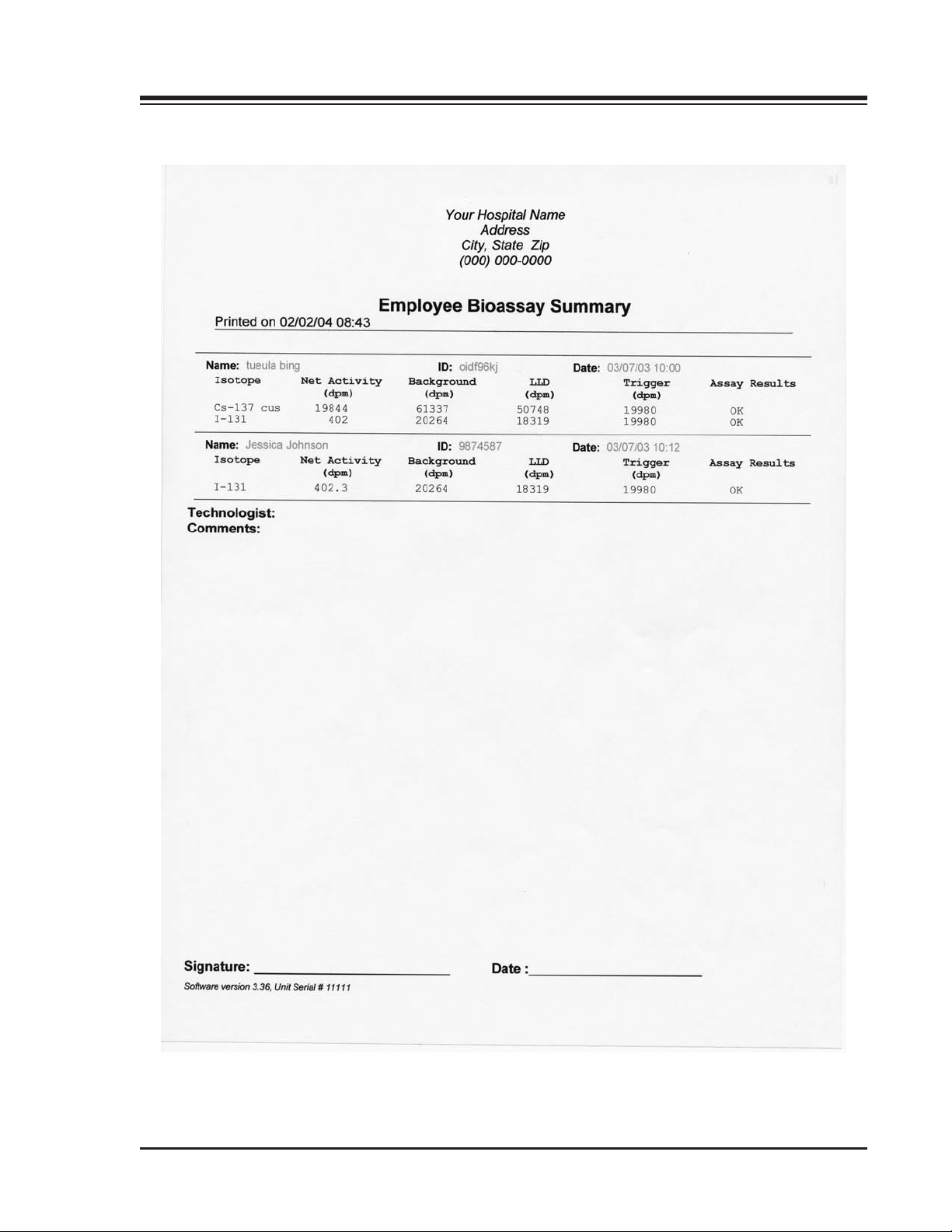
1. INTRODUCTION

Figure 7-5. An Individual Bioassay History Summary.

7-7 BIOASSAY

8. SCHILLING TESTS

In this mode, Schilling tests using the standard commercial kits Mallinckrodt - Bracco and Dicopac have
been programmed into the system. Before use, the operator should go to the Procedure Definition
Window, select the kit style used in the facility, and set-up or verify that the counting time, correction
factor and sample volumes are correct for the procedure.

For the Schilling Kits, the manufacturers recommend using a 4-ml sample volume with a correction factor
of 100 and a counting time of 600 seconds. This means that the standard, the sample and lab background
will all be counted for 600 seconds each (the correction factor deals with the standard). When the correct
parameters have been input into the kit procedure window, click on <Close>.

To Define a Facility Standard Schilling Test

(See Figure 8-1.)

To set up for the standard procedure used in your facility, it is helpful to set up a global facility standard
schilling test as described below.

1. Click on <Procedure Definition> in the primary tool bar. The procedure definition screen should now
be displayed.

2. Click on <Add>.

3. Enter the procedure name in the procedure name box.

4. Select the appropriate detector.

5. Select the Schillings Kit that you wish to use.

6. Enter the counting time.

7. Enter the proper correction factor.

8. Enter the sample volume to be counted.

9. Click <Save> to save the information.

NOTE: To change any information, click on <Open>. Select the appropriate type of procedure, whether it is
Thyroid Uptake, Schillings, or Hematology,and then select the appropriate study style under that procedure. If you
double click on the procedure, it will go to the procedure definition screen highlighting that particular procedure. If
you wish to enter a new procedure, follow the above procedure definition by clicking on <Add> and entering all the
appropriate information If you wish to just edit the procedure, click <Edit> and you can make any changes to the
procedure that you desire. It is recommended to add procedures to the list and delete the existing one if desired.

To Perform A Schillings Test (Bracco, Mallinckrodt or Simple
Mallinckrodt)

(See Figure 8-2.)

1. At the Patient Definition screen, choose an existing patient or enter a new patient.

2. Highlight the appropriate Schilling procedure to add this procedure to the selected patient. Once you
choose the procedure (i.e: Bracco Schilling Kit) click on <Select>. The Schilling counting page should
now be displayed.

8-1 SCHILLING TESTS

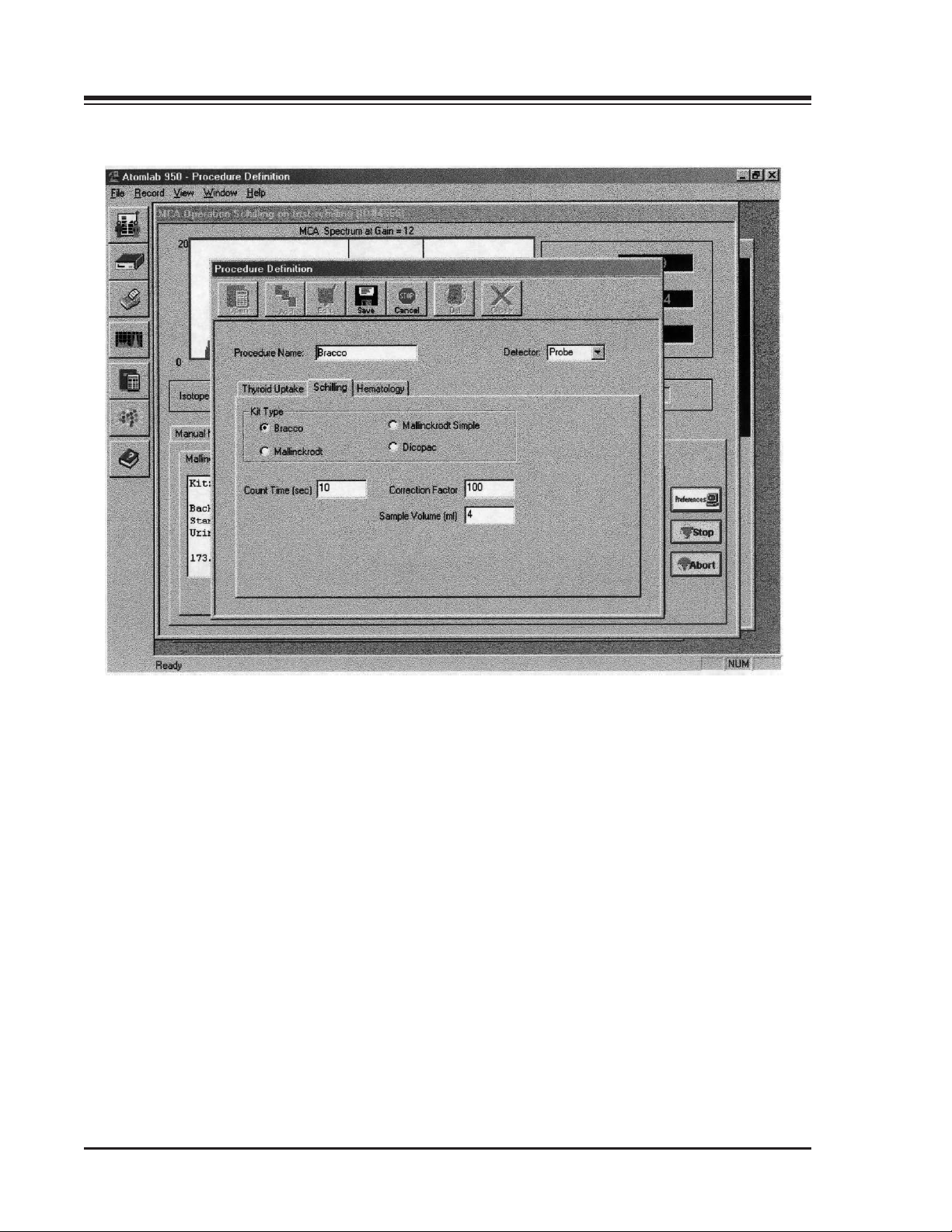
1. INTRODUCTION

Figure 8-1. Defining a Facility Standard Schilling Test.

SCHILLING TESTS 8-2

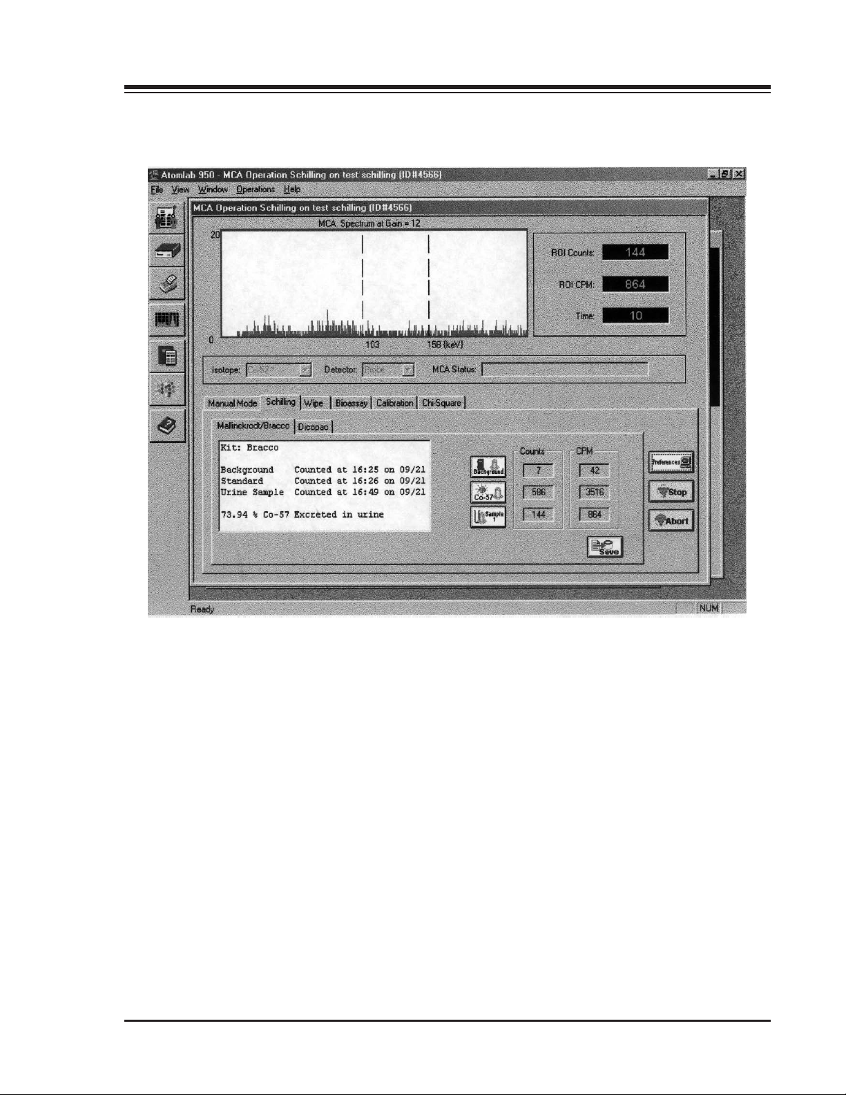
CONTENTS

Figure 8-2. The Schillings Counting Page.

8-3 SCHILLING TESTS

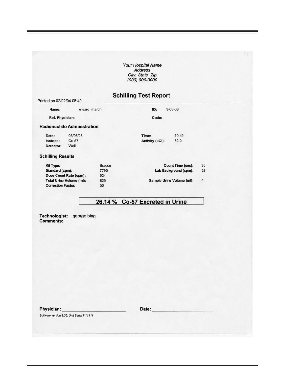
CONTENTS

Figure 8-3. A sample Schillings Mallinckrodt Report.

SCHILLING TESTS 8-4

CONTENTS

3. Click on the <Preferences> button and then enter a total urine volume for the patient that you are
testing. Once you have entered the total volume, click <OK>. You can now proceed with counting.

NOTE: You can change the sample volume, correction factor and count time for this study in the parameters
window.

NOTE: If you use a different standard volume or concentration, you must change the correction factor.

4. Click on the background button and the system will proceed to count lab background. When it is
done counting, the number of counts and the counts per minute will both be displayed.

5. Remove the background vial and insert the Co-57 standard into the well.

6. Click on the highlighted <Co-57> standard button. The system will now count the Co-57 standard.
When counting is finished, the total counts and the counts per minute will be displayed. The
<Sample> button should now be displayed.

7. Remove the Co-57 standard from the well and place the urine sample into the well.

8. Click on <Sample> to begin counting the urine sample. When counting is finished, the total counts
and counts per minute will be displayed.

9. When the system has completed the count, a window will be displayed asking to verify that the test
is complete. To save the results, click <Yes>. If you do not wish to Save, click <No> and you can
then proceed to recount any one of the three items counted.

NOTE: If an error was made in the total urine volume, do not click <Save>. You can go back and click on
<Preferences> to correct the error as long as you have not saved.

10. Once you have finished with any recounts for this patient, select <Save> to display the "Verify Test
Complete" screen. If the numbers are satisfactory, click <Yes> to save the results.

11. To print results at any time, click on the <Print> icon. This will open the report generation screen
from which you can choose a technologist to add to your study.

12. To enter and store the dose activity associated with this patient, press <Preview> for a preview of the
report. Press <Print> to print the report.

NOTE: Make sure to save before leaving the patient and going on to do other tests or studies with your
spectrometer.

NOTE: The Bracco and Mallinckrodt kits use the same procedure. You can modify the sample volumes, but
then you must correct and enter the appropriate sample volume in milliliters in the Preferences window.

Schilling Test for the Simplified Mallinckrodt Procedure

(See Figure 8-3.)

This is the same as the Mallinckrodt and Bracco procedures except that you cannot enter a sample
volume in the Preferences window. For this test, you must use a 4ml volume in order for the system to
calculate correctly.

Schilling Dicopac

(See Figures 8-4 and 8-5.)

The Dicopac Schillings procedure is programmed to use the Mediphysics/Amersham Dicopac Schilling
Test Kit. The counting procedures and formulas for calculations are all from the manufacturer's Dicopac
Kit instructions.

8-5 SCHILLING TESTS

CONTENTS

To Perform a Dicopac Schillings Test:

(See Figure 8-4.)

1. Click on the <Procedure> icon to access the Procedure Definition window.

2. At the Procedure Definition window, enter the parameters for the Dicopac studies that you wish to
perform. You can modify an existing procedure or create a new procedure. This entails entering the
counting time, sample volume, detector and type of kit.

NOTE: Once you do enter and save, this procedure is now stored and you do not have to enter it again.

3. Enter the patient, if not entered in the patient window, or select the patient if already in the system,
and pick the proper Schillings Test to perform for this patient.

4. At the Schilling Dicopac screen, verify that the patient name and ID is correct.

5. Click on <Preferences> to open the Dicopac parameters window.

6. Verify that the counting time and sample volumes are correct. The standard in the Dicopac Kit is 600
seconds counting time and a sample volume of 4ml.

7. Enter the total urine volume collected by the patient over the 24 hour collection period and click
<OK>.

8. Ensure the vials, samples and standards are ready and proceed with the test.

9. Take an empty vial and add water to it to the same volume that you are using for your urine aliquot.
Place this vial into the well counter.

10. Click <Background>. The system automatically counts background for both Co-57w and Co-58w.

11. Remove the tube used for background counting and place the Co-58 standard into the well counter.

12. Click on the < Co-58> standard button. The system will now count the Co-58 standard and record
the count in the Co-58w window. The system next automatically counts the Co-57w window, using
the Co-58 source to calculate spill-down.

NOTE: For spill-down, the system periodically pauses to record the current data, then continues counting from
0 counts (the time between data downloads varies depending on the count rate). New data is added to previous
data until the total counting time requested is completed. This prevents roll-over from occurring. The total
counts for spill-down are recorded as the final Co-57 spill-down result.

13. Remove the Co-58 standard from the well counter.

14. Place the Co-57 standard into the well counter.

15. Click <Co-57>to count the Co-57 standard and store the value. When done counting, remove the Co­57 standard from the well counter.

16. Place the urine aliquot or sample into the well counter.

17. Click on <Sample> to count the urine sample for both the Co-58w and Co-57w windows.

18. When counting, is complete, the "Verified Test Complete” window is displayed. At this point, the
system displays the calculations for Co-57, Co-58 and the percentage excretion in the lower left corner
of the screen. If you wish to save, click <Yes>. The system will automatically save the data.

SCHILLING TESTS 8-6

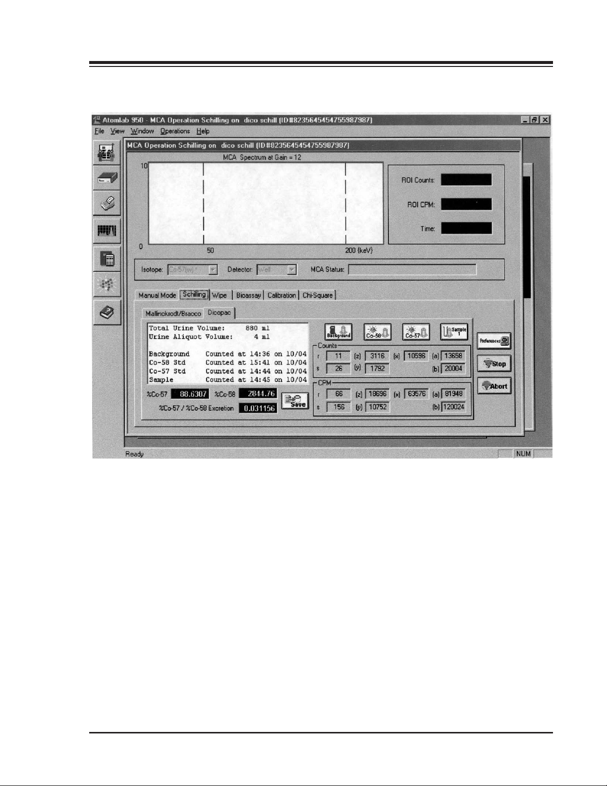
CONTENTS

Figure 8-4. The Diopac Schillings Counting Page.

8-7 SCHILLING TESTS

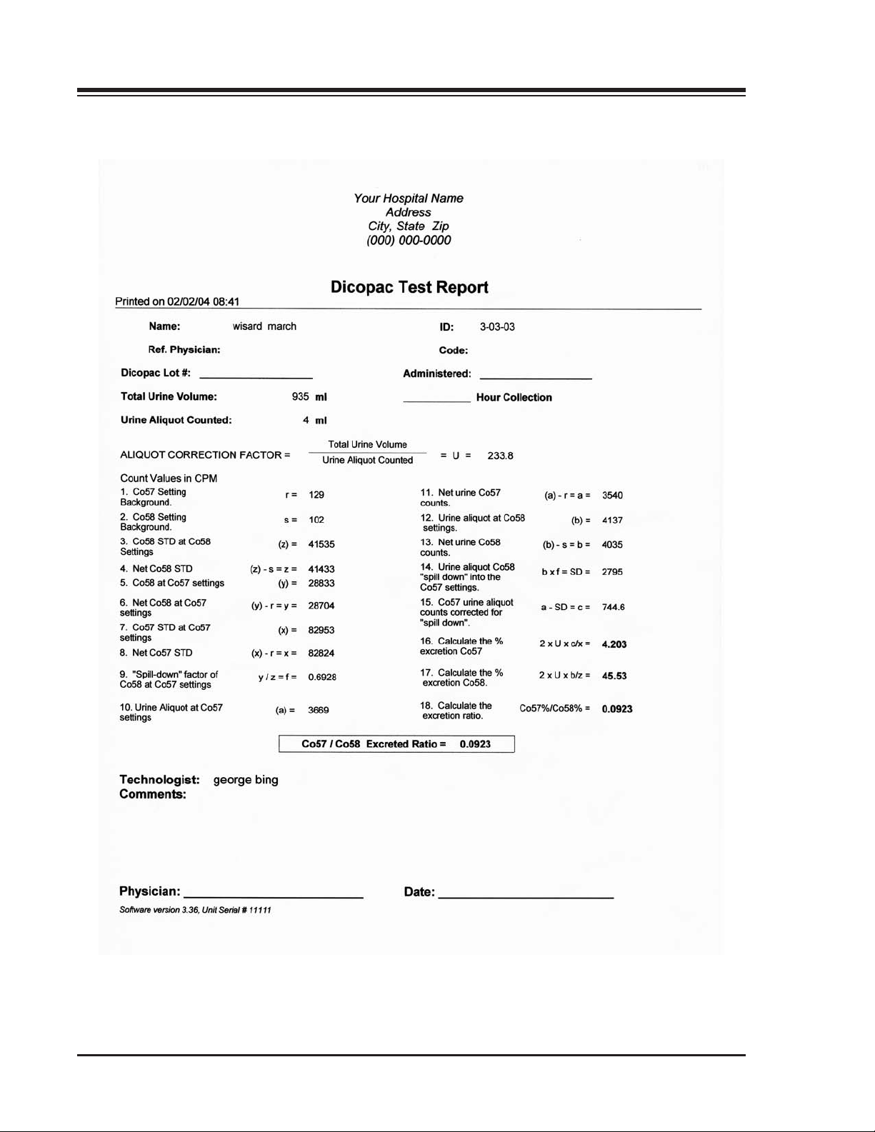
CONTENTS

Figure 8-5. A Sample Diopac Schillings Report.

SCHILLING TESTS 8-8

9. HEMATOLOGY

In the Hematology Mode there are a number of different programs that can be used. All are based on
commercially available kits. The programs include IHSA I-125, Cr-51 Blood Volume, Cr-51 Red Cell
Survival, Glomerular Filtration Rate (GFR) and Effective Renal Plasma Flow (ERPF).

The Hematology Patient Page

(See Figure 8-1.)

Setting Up For Hematology

1. To set up for any of the hematology procedures, click on the <Procedure Definition> icon in the
primary tool bar to select the Procedure Definition window.

2. Open the procedure list and correct or change any parameters for any procedure or create a new
procedure with the requirements for your studies.

NOTE: Once you have created the standard procedure for this study, you do not have to go back to this
window and modify it. It will be stored and usable for any future patient studies of this type.

3. Click on the <Patient Definition> icon in the primary tool bar. The Patient Definition window should
now be displayed. For an existing patient, simply add the new procedure. For a new patient, add the
patient and the procedure.

NOTE: We recommended creation of a new procedure rather than modification of an existing procedure.

4. Once a patient is in the system and the appropriate hematology method is listed for that patient,
select that patient and proceed to the Hematology Counting page. You can now proceed to the
appropriate test as described below.

IHSA I-125

(See Figure 9-1 and 9-2.)

To perform an IHSA I-125 study, follow the kit instructions for preparing and administering the dose.
When preparing to count the different parts of the study, be sure to have all the vials set up so they can be
counted one after the other to negate any decay factors.

1. To start the study, verify that the correct patient and patient ID# is listed at the top of the
Hematology Counting page.

2. Click on <Preferences> at the right side of the screen and verify the volumes and dosage used.
Correct the count time if desired. After reviewing the window and parameters, click <OK>.

3. Click on <Background> to perform a background count for the I-125 window. When done counting, the
system will display the counts and CPM. The <Iodine Standard> button should now be highlighted.

4. Remove the vial that was used for counting background and place the vial with the iodine standard
into the well counter. Click on <Iodine Standard> to count the standard. When done counting the
system will display the counts and the counts per minute.

5. Remove the vial with the iodine standard and place the blood sample vial into the well counter.

6. Click on <Blood Sample> to begin counting the blood sample. When done counting, the system
displays the counts and CPM for the blood sample.

7. Remove the blood sample vial from the well counter and put the plasma sample vial into the
well counter.

9-1 HEMATOLOGY

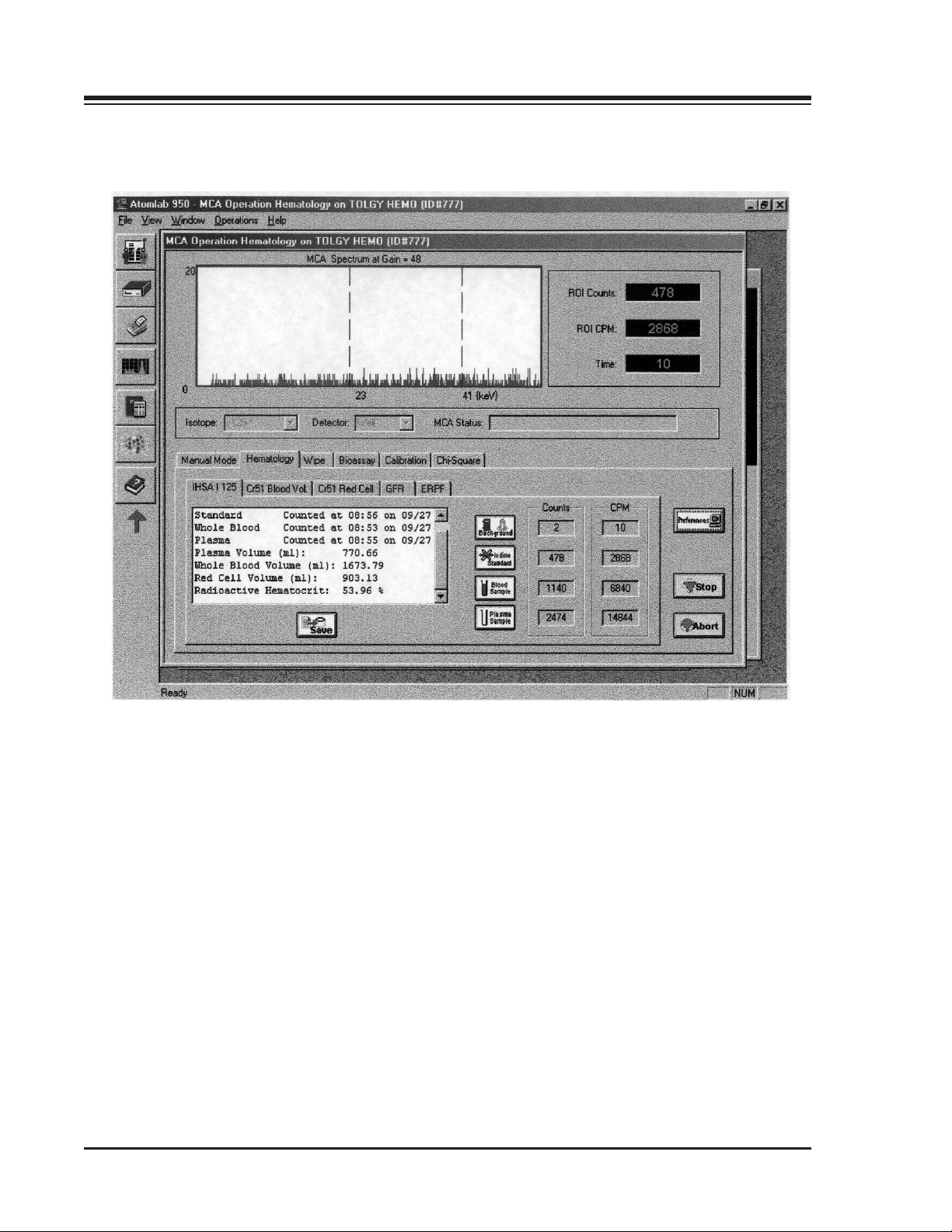
CONTENTS

9-1. The IHSA Counting Page.

HEMATOLOGY 9-2

CONTENTS

8. Click on <Plasma Sample> to begin counting the plasma sample. When done counting, the system
displays the plasma sample counts and count rate.

9. When it is done counting the plasma sample, the system will display the "Verified Test Complete"
window, asking if you want to permanently save the data. In the lower left corner of the screen you
can see the calculations and results for the volumes and radioactive hematocrit percent number. To
accept the numbers that were taken, click <Yes> to save the data. If you wish to recount any of the
items, click <No>.

10. If you are satisfied with the results, click <Yes> on the "Verified Test Complete" screen (if this screen
is not displayed, click on <Save> to bring up the screen, then click <Yes> to save before moving onto
any other patients or functions.

NOTE: Once you have saved, you cannot make any other changes to this particular study for this patient.

NOTE: If you wish to print a report, click on the <Printer> icon in the primary tool bar and then print the
appropriate hematology report. You can add a technologist and a dose activity to the report, if desired.

Cr-51 Blood Volume

(See Figure 9-3.)

To perform a Cr-51 blood volume test, prepare all your samples and label them according to the
manufacturer's kit instructions. When you are ready to count, you must first enter a patient into the
patient database and choose the Cr-51 blood volume test for that patient. If the patient is already in the
system, add a new test of the Cr-51 blood volume as a new procedure for this patient.

A one-time set up for the Cr-51 test would be to go to the procedure window and enter the count time
that you will use for each of the items into the procedure definition. Once this time is set and you save it,
all Cr-51 blood volume tests will use this counting time, unless adjusted.

1. At the Cr-51 blood volume counting page, verify that the patient Name and patient's ID# at the top of

the screen are correct.

2. Click on <Preferences> and enter the patient hematocrit number as a percentage. Also enter the Red

Blood Cell (RBC) suspension hematocrit as a percentage. If needed, adjust the counting time in this
window and then press <OK> to proceed.

3. Place the vial that will be used for counting background into the well counter and click on

<Background>. The system will now count for background. When counting is completed, the counts
and counts per minute will be displayed.

4. Remove the background vial from the well and insert the vial with the blood standard into the well

counter. Click on <Blood Standard> count the standard. When counting is completed, the counts and
counts per minute will be displayed.

5. Remove the blood standard vial from the well counter and insert the plasma standard vial into the

well counter. Click <Plasma Standard> to count the plasma standard. When counting is completed,
the counts and counts per minute for the plasma standard will be displayed.

6. Remove the plasma standard vial from the well counter and put the blood sample vial into the well

counter. Click on <Blood Sample> to count the blood sample. When counting is completed, the
counts and counts per minute for the blood sample will be displayed.

7. Remove the blood sample vial from the well counter and place the plasma sample vial into the well

counter. Click on <Plasma Sample> to count the plasma sample. When counting is completed, the
counts and counts per minute for the plasma sample will be displayed.

9-3 HEMATOLOGY

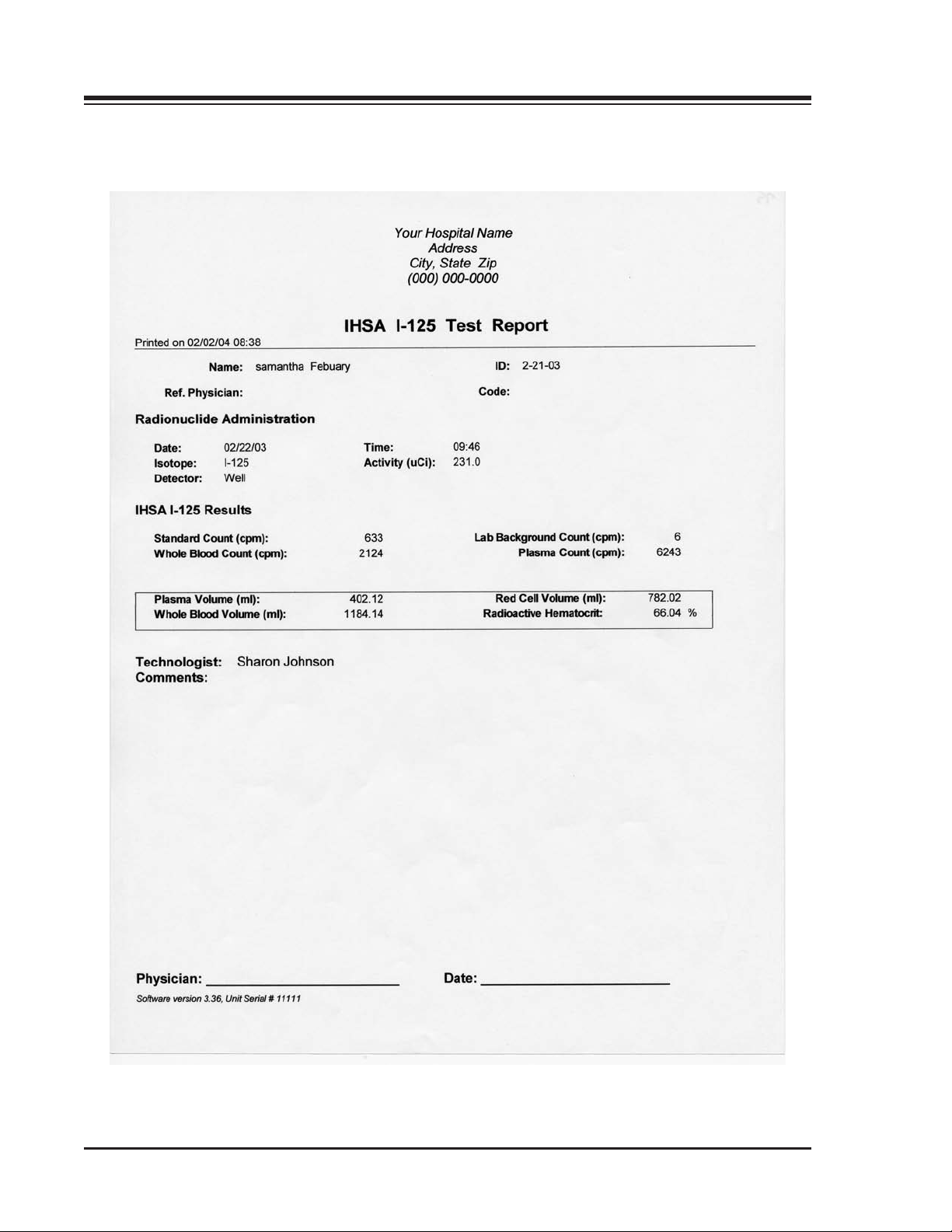
1. INTRODUCTION

Figure 9-2. A Sample IHSA I-125 Test Report.

HEMATOLOGY 9-4

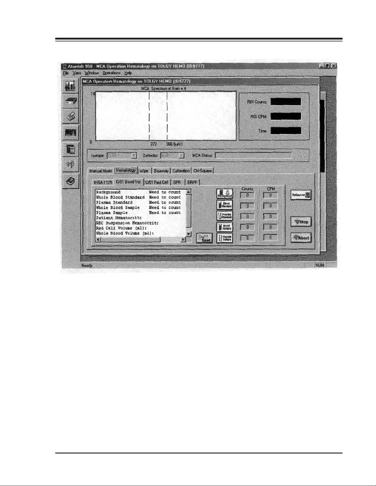
CONTENTS

Figure 9-3. The CR-51 Counting Page.

9-5 HEMATOLOGY

CONTENTS

8. When it is done counting the plasma sample, the system will display the "Verified Test Complete"
window, advising that the test is complete and you can now permanently save the results in the
database. If you are satisfied with the results and the tests, click <Yes> to permanently save. If you
wish to recount any one of the items, click <No>.

9. If you have clicked <No>, you can now place the appropriate vial into the well and press the
corresponding button to recount that vial. When the system is done it will display the "Verified Test
Complete" window again and you can save or not save at that point.

NOTE: If you did not save and you are looking at the Cr-51 main screen, you can save by pressing the <Save>
button, which will display the <Verified Test Complete> screen. Then click <Yes> and the study will be
permanently saved. You can now proceed to count another patient or do another procedure.

HEMATOLOGY 9-6

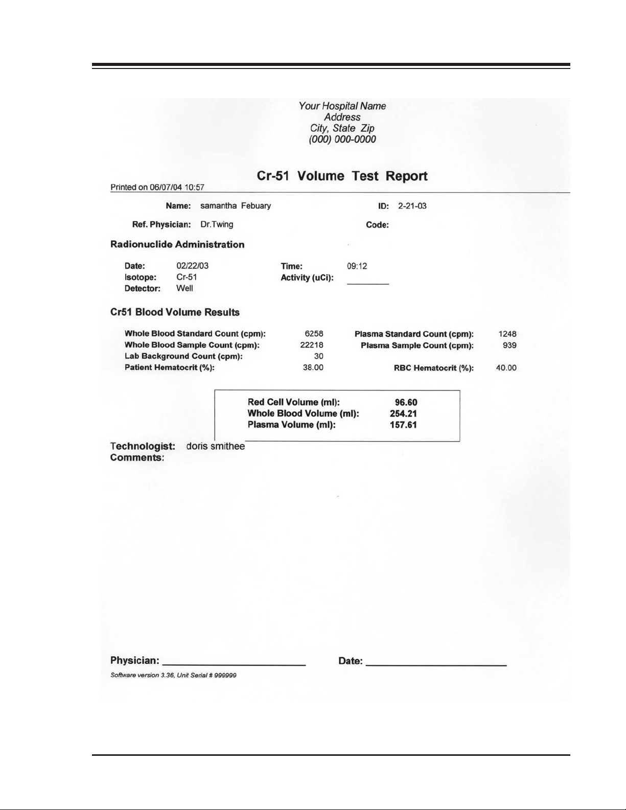
CONTENTS

Figure 9-4. A Sample Cr-51 Volume Test Report.

9-7 HEMATOLOGY

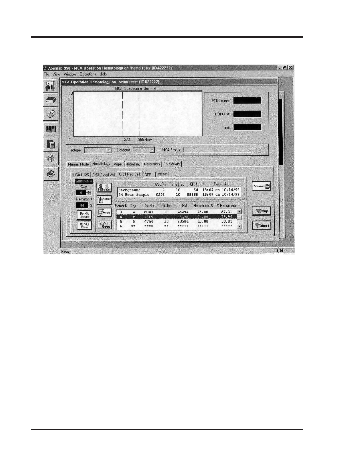
CONTENTS

Figure 9-5. The Cr-51 Red Blood Cell Survival Counting Page.

HEMATOLOGY 9-8

CONTENTS

Cr-51 Red Cell Survival

(See Figures 9-5 and 9-6.)

To set up as the standard number of samples and the count time, click on the <Procedure Definition> icon
in the primary tool bar and then enter the red cell survival maximum number of samples and counting
time. Once set, these will be the default values for each new study performed.

NOTE: This information in <Procedure Definition> can be set-up anytime for all procedures before counting any
patients. These are your default counting parameters.

The Cr-51 Red Cell Survival test follows the procedures from the published Mallinckrodt Red Cell
Survival Test Kit. In order to perform this test, assemble all the blood samples, appropriate hematocrits,
the standard, and a background vial to count. When entering the data for this test, enter the hematocrit
that is associated with each sample number as well as entering the day the sample was drawn (i.e.,
sample drawn after 72 hours is Day 3.) Since the Red Cell Survival Test stretches over many days, there
can be days skipped between when samples are drawn.

To perform a Red Cell Survival Test:

1. Either enter a new patient and pick the Red Cell Survival procedure for this patient, or go to the Patient
Window, select the existing patient and add the Red Cell Survival as a new test for this patient. Once
the patient has been set up for the Red Cell Survival, proceed to the counting screen for this patient.

2. At the counting screen, verify that the correct patient and ID# are on the page.

3. Click on <Preferences>. In the preferences window is displayed the counting time and the number
of samples to be counted. You can correct the number of samples and increase or decrease the
numbers as desired. Once you have set the count time and the number of samples, click <OK>. You
can now proceed to count.

4. Put the background vial into the well counter and click <Background>. The system will count the
background for the pre-determined time. When done, the counts per minute and the counting time,
plus the time/date that background was counted will be displayed.

5. After background is counted, the system will highlight the 24 hour sample. Remove the background
vial from the well counter and place the vial with the 24 hour sample into the well counter.

6. On the left side of the page is displayed Sample #1, Day #1 and hematocrit as 0%. Enter a value for
hematocrit by first double clicking on the box and then typing in the correct value for Sample
#1 Hematocrit.

7. Click on <Sample> to count the 24 hour blood sample. When done counting, the system will display
and enter the counts, counting time and hematocrit into the chart.

8. When it is finished counting, the system will proceed to Sample #2. Remove Sample #1 and put
Sample #2 into the well counter.

9. On the left side of the screen is displayed Sample #. Below that, the day is listed as zero and hematocrit
is listed as zero. Using the <UP/DOWN Arrows>, set the day to match the day on which the sample
was drawn. Enter the hematocrit number by first double clicking on the box and then entering the
appropriate hematocrit. When you are done entering hematocrit as a percentage, click on <Sample>.
The system will now count Sample #2. When it is done counting, the results will be displayed.

10. The system will now advance to the third sample and display Sample #3 on the left side of the
screen. Using the <UP/DOWN Arrows>, enter the day the sample was drawn. Now enter the
hematocrit value by double clicking on the box and then entering the hematocrit as a percentage.

9-9 HEMATOLOGY

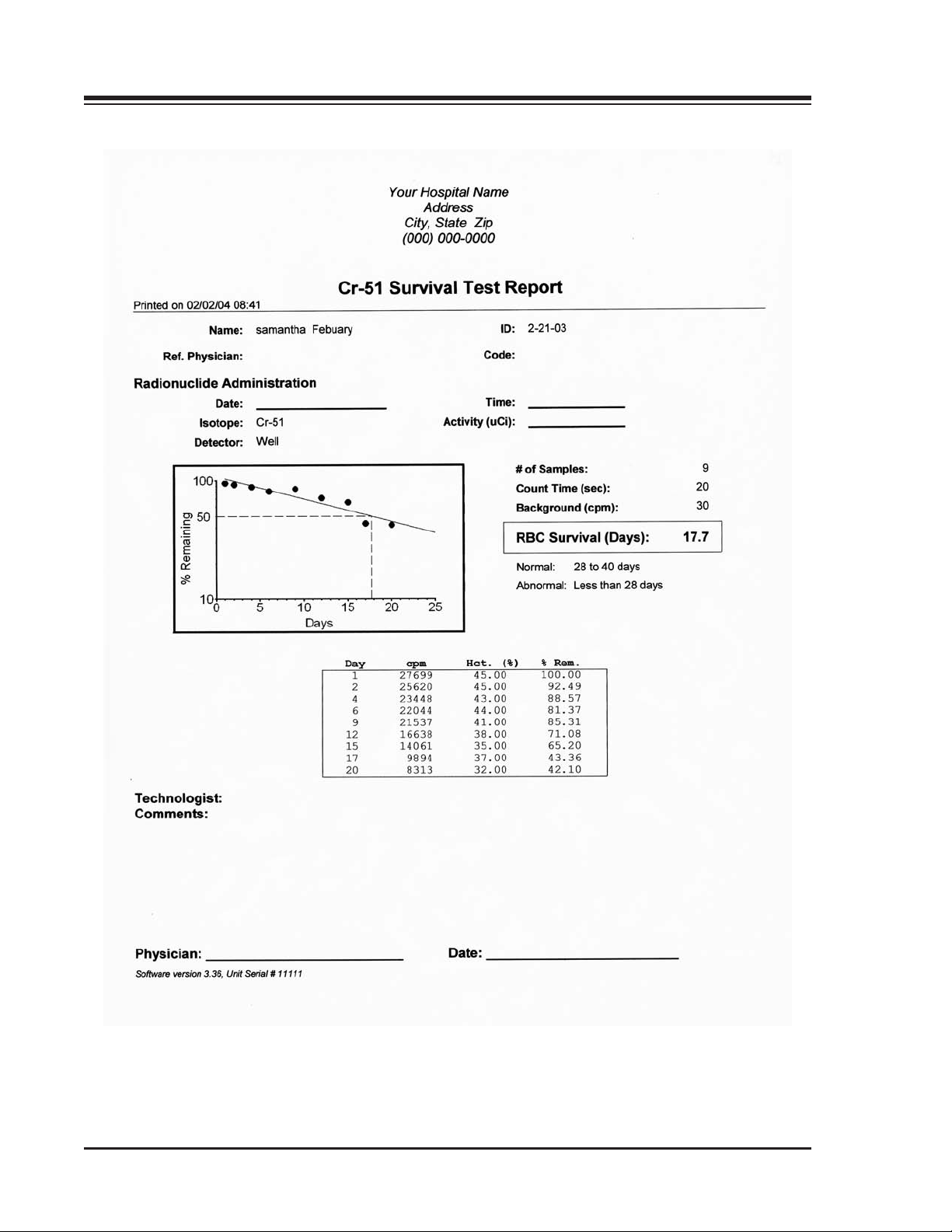
CONTENTS

Figure 9-6. A sample Cr-51 Survival Test Report.

HEMATOLOGY 9-10

CONTENTS

GFR

(See Figure 9-7.)

The following test is for the Glomerular Filtration Rate (GFR) test. This test uses Technetium-99m - DTPA
as the pharmaceutical. The GFR test is a renal function test of the kidneys. The procedure followed is
from the Journal of Nuclear Medicine Technology, Volume 14, Number 4, December 1986, entitled,
"Technical Aspects of a New Technique for Estimating Glomerular Filtration Rate Using Technetium-99m

- DTPA" by Kathrine R. Rowell, Frances N. Kontzen, Marian E. Stutzman, et al., V.A. Medical Center and

University of Alabama, Birmingham, Alabama. The program can have either one or two samples used in
the calculation.

Both the one and two sample methods follow the package inserts for Technetium DTPA for production of
the pharmaceutical. Look at the HELP SECTION for the Medical Spectrometer. There is a reproduction
of the procedure from the above mentioned article. The following instructions are for use of the Multi­Channel Analyzer for counting the standard and sample(s) for getting your results.

GFR One Sample Method

(See Figure 9-8.)

1 At the <Patient Definition> window, enter a new patient and choose the appropriate GFR One

Sample or Two Sample test for an existing patient, or enter a new patient and choose the appropriate
GFR test.

2. Click on the Hematology Counting tab to bring up the counting screen. Verify that the patient and
ID# are correct.

3. Click on <Preferences> and find the standard to dilution ratio and quantity used to count for both
the standard and the ultra filtrate. If you wish to enter any parameter, it should be done before
counting. Now click <OK> to close the GFR parameters window. Any changes will now be
implemented.

4. Clear away any radioactive sources from near the well counter. If you have not calibrated the well
counter today, do so now.

5. Place a test tube or vial similar to what you were using for the other samples to be tested into the
well counter. This will be used for background testing.

6. Click on <Background> and the system will proceed to count background. When done counting, it
will display the counts and the CPM.

7. Remove the background counting vial from the well counter and place the standard into the well
counter. Click on <Standard> to count the standard. When done counting, the system displays the
counts and the CPM.

8. Click on <Inject> to enter the time and date of injection. If you click on <Now>, it will bring the time
and date to the current date and time. You can then change this to whatever is appropriate. Click on
<OK> to set the date and time.

9. Click on <Time /Sample 1> and enter the time that the sample was drawn. Once you have entered
the time for the sample, click <OK> to record it. If you do not wish to save it, click <Cancel>.

NOTE: The GFR procedure calls out for a 3 hour sample withdrawal following the injection of the
pharmaceutical.

10. Place the sample into the well counter and click on <Sample>. The system will now count the
sample for the appropriate time and, when finished, display the counts and CPM.

9-11 HEMATOLOGY

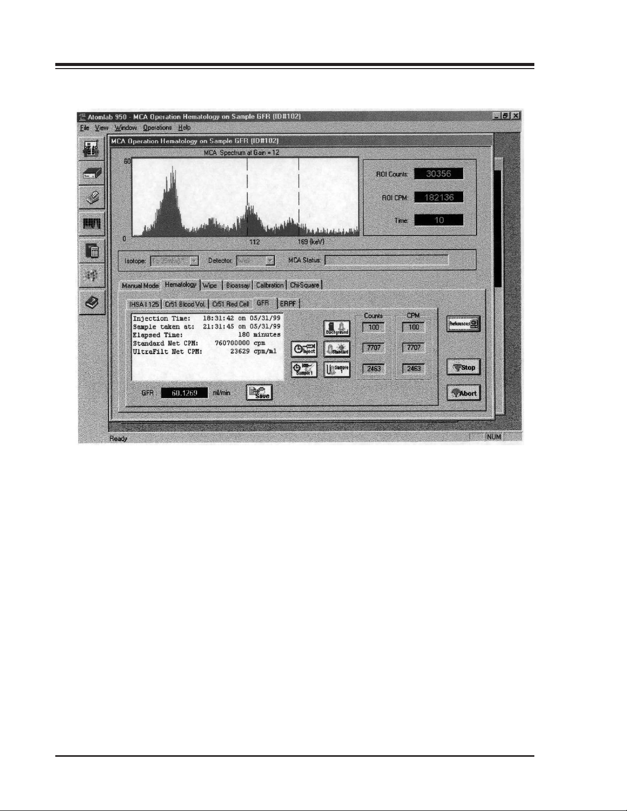
CONTENTS

Figure 9-7. The GFR Counting Page.

HEMATOLOGY 9-12