

Page 1
User´s Guide
VCXG (Gigabit Ethernet) / VCXU (USB 3.0)
Document Version: v1.1
Release: 07.06.2016
Document Number: 11165414
Page 2

2
Page 3

3
Table of Contents
1. General Information ................................................................................................. 6
2. General safety instructions ..................................................................................... 7
3. Intended Use ............................................................................................................. 7
4. General Description ................................................................................................. 8
4.1 VCXG ...................................................................................................................... 9
4.2 VCXU ...................................................................................................................... 9
5. Camera Models ....................................................................................................... 10
5.1 VCXG .................................................................................................................... 10
5.2 VCXU .....................................................................................................................11
6. Installation .............................................................................................................. 12
6.1 Environmental Requirements ................................................................................ 12
6.2 Heat Transmission ................................................................................................ 13
6.3 Mechanical Tests ................................................................................................... 14
7. Pin-Assignment / LED-Signaling .......................................................................... 15
7.1 VCXG .................................................................................................................... 15
7.1.1 Ethernet Interface (PoE) ................................................................................. 15
7.1.2 Power Supply and IOs .................................................................................... 15
7.1.3 GPIO (General Purpose Input/Output) ........................................................... 15
7.1.4 Digital IO ......................................................................................................... 16
7.1.5 LED Signaling ................................................................................................. 16
7.2 VCXU .................................................................................................................... 17
7.2.1 USB 3.0 Interface ........................................................................................... 17
7.2.2 Digital IOs ....................................................................................................... 18
7.2.3 GPIO (General Purpose Input/Output) ........................................................... 18
7.2.4 Digital IO ......................................................................................................... 18
7.2.5 LED Signaling ................................................................................................. 19
8. ProductSpecications .......................................................................................... 20
8.1 Spectral Sensitivity ................................................................................................ 20
8.2 Field of View Position ............................................................................................ 22
8.2.1 VCXG ............................................................................................................. 22
8.2.2 VCXU.............................................................................................................. 22
8.3 Acquisition Modes and Timings ............................................................................. 23
8.3.1 Continuous Mode (Free Running Mode) ........................................................ 23
8.3.2 Single Frame Mode ........................................................................................ 24
8.3.3 Multi Frame Mode........................................................................................... 24
8.3.4 Acquisition Frame Rate Mode ........................................................................ 24
8.3.5 Trigger Mode .................................................................................................. 25
8.3.6 Advanced Timings for GigE Vision
®
/USB3 VisionTM Message Channel .......... 29
Page 4

4
8.4 Software ................................................................................................................ 32
8.4.1 Baumer GAPI ................................................................................................. 32
8.4.2 3
rd
Party Software ........................................................................................... 32
9. Camera Functionalities .......................................................................................... 33
9.1 Image Acquisition .................................................................................................. 33
9.1.1 Image Format ................................................................................................. 33
9.1.2 Pixel Format ................................................................................................... 34
9.1.3 Exposure Time................................................................................................ 36
9.1.4 Fixed Pattern Noise Correction (FPNC) ......................................................... 37
9.1.5 Look-Up-Table ................................................................................................ 38
9.1.6 Gamma Correction ......................................................................................... 38
9.1.7 Region of Interest ........................................................................................... 39
9.1.8 Binning............................................................................................................ 40
9.1.9 Brightness Correction ..................................................................................... 43
9.1.10 Flip Image ..................................................................................................... 44
9.2 Color Processing ................................................................................................... 45
9.3 Color Adjustment – White Balance ....................................................................... 45
9.3.1 User-specic Color Adjustment ...................................................................... 45
9.3.2 One Push White Balance (Once) ................................................................... 46
9.3.3 Continuous White Balance ............................................................................. 46
9.4 Analog Controls ..................................................................................................... 46
9.4.1 Offset / Black Level ......................................................................................... 46
9.4.2 Gain ................................................................................................................ 47
9.5 Pixel Correction ..................................................................................................... 48
9.5.1 General information ........................................................................................ 48
9.5.2 Correction Algorithm ....................................................................................... 49
9.5.3 Defectpixellist ................................................................................................. 49
9.6 Process Interface .................................................................................................. 50
9.6.1 Digital IOs ....................................................................................................... 50
9.6.2 Trigger ............................................................................................................ 53
9.6.3 Trigger Source ................................................................................................ 53
9.6.4 Debouncer ...................................................................................................... 54
9.6.5 ExposureActive (Flash Signal) ....................................................................... 54
9.6.6 Timers ............................................................................................................. 55
9.6.7 Frame Counter ............................................................................................... 55
9.7 Device Reset ......................................................................................................... 56
9.8 User Sets .............................................................................................................. 56
9.8.1 VCXG ............................................................................................................. 56
9.8.2 VCXU.............................................................................................................. 57
9.9 Factory Settings .................................................................................................... 57
9.10 Timestamp .......................................................................................................... 58
9.11 Chunk .................................................................................................................. 59
10. VCXG - Interface Functionalities ........................................................................... 60
10.1 Device Information .............................................................................................. 60
10.2 Packet Size and Maximum Transmission Unit (MTU) ......................................... 60
10.3 Inter Packet Gap (IPG) ....................................................................................... 60
10.3.1 Example 1: Multi Camera Operation – Minimal IPG ..................................... 61
10.3.2 Example 2: Multi Camera Operation – Optimal IPG ..................................... 61
10.4 Transmission Delay ............................................................................................. 62
10.4.1 Time Saving in Multi-Camera Operation ...................................................... 62
10.4.2 Conguration Example ................................................................................. 63
Page 5

5
10.5 Multicast .............................................................................................................. 65
10.6 IP Conguration .................................................................................................. 66
10.6.1 Persistent IP ................................................................................................. 66
10.6.2 DHCP (Dynamic Host Conguration Protocol) ............................................. 66
10.6.3 LLA ............................................................................................................... 67
10.6.4 Force IP ........................................................................................................ 67
10.7 Packet Resend .................................................................................................... 68
10.7.1 Normal Case................................................................................................. 68
10.7.2 Fault 1: Lost Packet within Data Stream ...................................................... 68
10.7.3 Fault 2: Lost Packet at the End of the Data Stream ..................................... 68
10.7.4 Termination Conditions ................................................................................. 69
10.8 Message Channel ............................................................................................... 70
10.8.1 Event Generation ......................................................................................... 70
10.9 Action Command / Trigger over Ethernet ............................................................ 71
10.9.1 Example: Triggering Multiple Cameras ........................................................ 71
11. VCXU - Interface Functionalities ........................................................................... 72
11.1 Device Information .............................................................................................. 72
11.2 Message Channel ............................................................................................... 73
11.2.1 Event Generation .......................................................................................... 73
11.3 Chunk ................................................................................................................. 74
12. Start-Stop-Behaviour ............................................................................................. 75
12.1 Start / Stop / Abort Acquisition (Camera) ............................................................ 75
12.2 Start / Stop Interface ........................................................................................... 75
13. Cleaning .................................................................................................................. 76
14. Transport / Storage ................................................................................................ 76
15. Disposal .................................................................................................................. 76
16. Warranty Notes ....................................................................................................... 77
17. Support .................................................................................................................... 77
18. Conformity .............................................................................................................. 77
18.1 CE ....................................................................................................................... 77
18.2 RoHS .................................................................................................................. 77
Page 6

6
1. General Information
Thanks for purchasing a camera of the Baumer family. This User´s Guide describes how
to connect, set up and use the camera.
Read this manual carefully and observe the notes and safety instructions!
Target group for this User´s Guide
This User's Guide is aimed at experienced users, which want to integrate camera(s) into
a vision system.
Copyright
Any duplication or reprinting of this documentation, in whole or in part, and the reproduc-
tion of the illustrations even in modied form is permitted only with the written approval of
Baumer. This document is subject to change without notice.
Classicationofthesafetyinstructions
In the User´s Guide, the safety instructions are classied as follows:
Notice
Gives helpful notes on operation or other general recommendations.
Caution
Pictogram
Indicates a possibly dangerous situation. If the situation is not avoided, slight
or minor injury could result or the device may be damaged.
Page 7
7
2. General safety instructions
Caution
Heat can damage the camera. Provide adequate dissipation of heat, to
ensure that the temperature does not exceed the value (see Heat Transmission).
As there are numerous possibilities for installation, Baumer recommends
no specic method for proper heat dissipation, but suggest the following
principles:
▪ operate the cameras only in mounted condition
▪ mounting in combination with forced convection may provide proper heat
dissipation
Caution
Observe precautions for handling electrostatic sensitive devices!
Caution
Class A
The camera is a class A device (DIN EN 55022:2011). It can cause radio
interference in residential environments. Should this happen, you must take
reasonable measures to eliminate the interference.
3. Intended Use
The camera is used to capture images that can be transferred over a GigE interface
(VCXG) or a USB 3.0 interface (VCXU) to a PC.
Page 8

8
4. General Description
All Baumer cameras of these families are characterized by:
Best image quality ▪ Low noise and structure-free image information
▪ High quality mode with minimum noise
Flexible image acquisition ▪ Industrially-compliant process interface with parameter
setting capability
Fast image transfer VCXG ▪ Reliable transmission up to 1000 Mbit/sec
according to IEEE802.3
▪ Cable length up to 100 m
▪ PoE (Power over Ethernet)
▪ Baumer driver for high data volume with low
CPU load
▪ High-speed multi-camera operation
▪ GenICam™ and GigE Vision
®
compliant
VCXU ▪ Reliable transmission at 5000 Mbit/sec
according to USB 3.0 (v1.0) standard
▪ GenICam™ and USB3 Vision
TM
compliant
Perfect integration ▪ Flexible generic programming interface (Baumer GAPI)
for all Baumer cameras
▪ Powerful Software Development Kit (SDK) with sample
codes and help les for simple integration
▪ Baumer viewer for all camera functions
▪ GenICam™ compliant XML le to describe the camera
functions
▪ Supplied with installation program with automatic
camera recognition for simple commissioning
Compact design ▪ Light weight
▪ exible assembly
Reliable operation ▪ State-of-the-art camera electronics and precision
mechanics
▪ Low power consumption and minimal heat generation
Supported Standards VCXG ▪ v2.0 (v1.2 backward compatible)
▪ GenICam SFNC 2.1
VCXU ▪ USB3 Vision
TM
1.0.1
▪ GenICam GenCP 1.1
▪ GenICam SFNC 2.1
Page 9
9
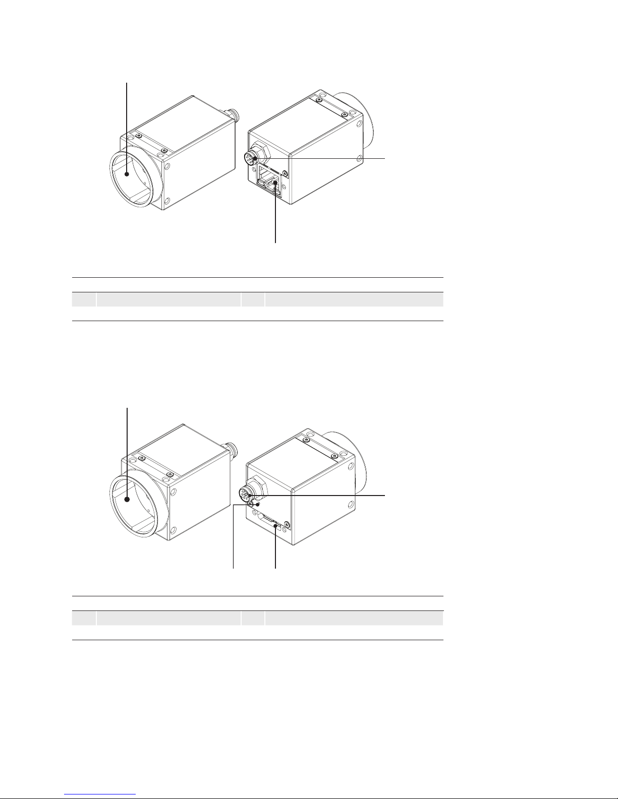
4.1 VCXG
2
3
1
No. Description No. Description
1 Lens mount (C-Mount) 3 Ethernet Port (PoE) / Signaling LED´s
2 Power supply / Digital-IO
4.2 VCXU
2
43
1
No. Description No. Description
1 Lens mount (C-Mount) 3 USB 3.0 port
2 Digital-IO 4 Signaling-LED
Page 10
10
5. Camera Models
5.1 VCXG
Camera Type
Sensor
Size
Resolution
Full
Frames1)
[max. fps]
Monochrome
VCXG-53M 1" 2592 x 2048 28 ׀ 23
Color
VCXG-53C 1" 2592 x 2048 28 ׀ 23
1)
Burst Mode (image acquisition in the camera´s internal memory) ׀ interface
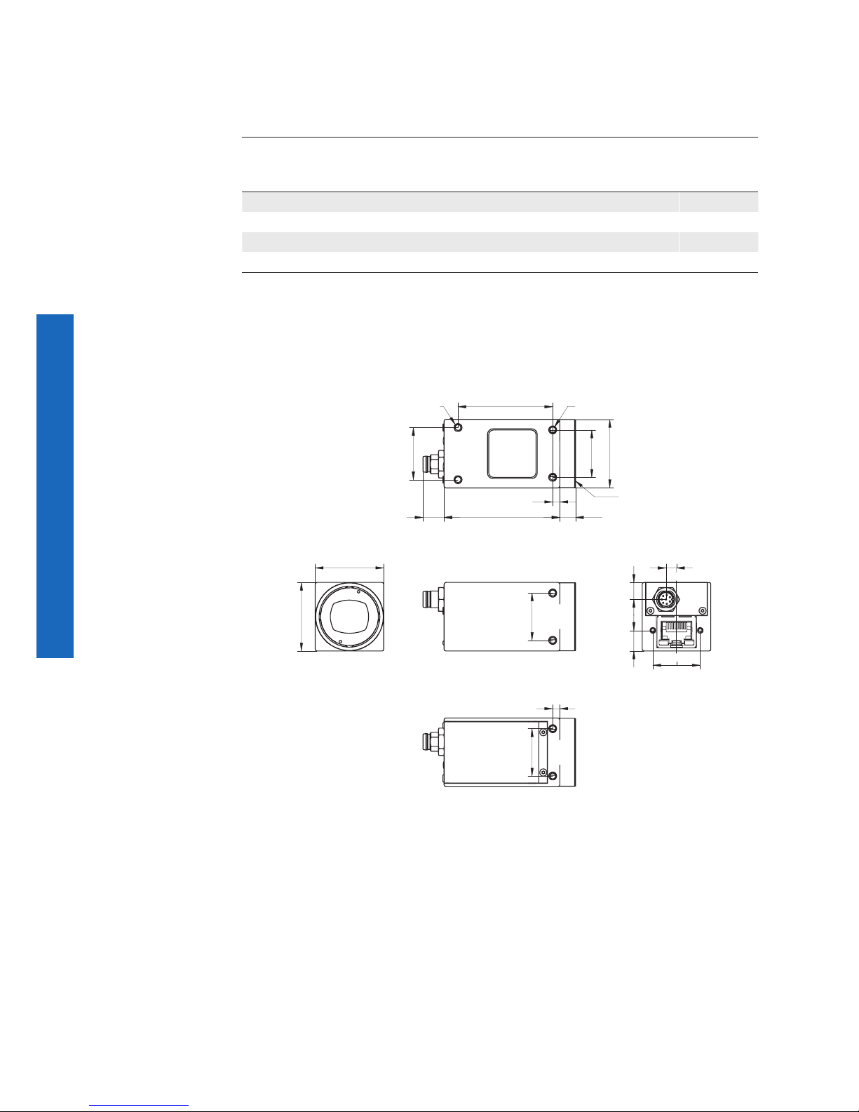
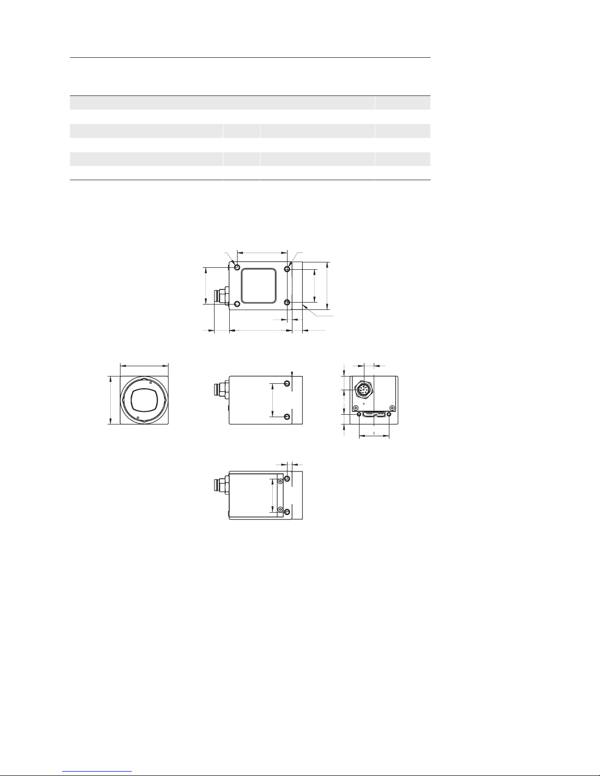
Dimensions
29
29
20
20
4,45
7,2
8,7
20
3
28,7
20
22
40
C-Mount
6,648,98,9
3
8 x M3 x 4
2 x M3 x 4
ø
Page 11
11
5.2 VCXU
Camera Type
Sensor
Size
Resolution
Full
Frames
[max. fps]
Monochrome
VCXU-23M 1/1.2" 1920 x 1200 165
VCXU-50M 2/3" 2448 x 2048 76
Color
VCXU-23C 1/1.2" 1920 x 1200 165
VCXU-50C 2/3" 2448 x 2048 76
Dimensions
29
29
20
18
6,15
8,2
6
20
3
28,7
20
22
30
C-Mount
6,2537,88,9
3
8 x M3 x 4
2 x M3 x 4
ø
Page 12

12
6. Installation
Lens mounting
Notice
Avoid contamination of the sensor and the lens by dust and airborne particles when
mounting the lens to the device!
Therefore the following points are very important:
▪ Install the camera in an environment that is as dust free as possible!
▪ Keep the dust cover (bag) on camera as long as possible!
▪ Hold the camera downwards with unprotected sensor.
▪ Avoid contact with any optical surface of the camera!
6.1 Environmental Requirements
Temperature
Storage temperature -10°C ... +70°C ( +14°F ... +158°F)
Operating temperature* see „6.2 Heat Transmission“
Humidity
Storage and Operating Humidity 10% ... 90%
Non-condensing
Page 13
13
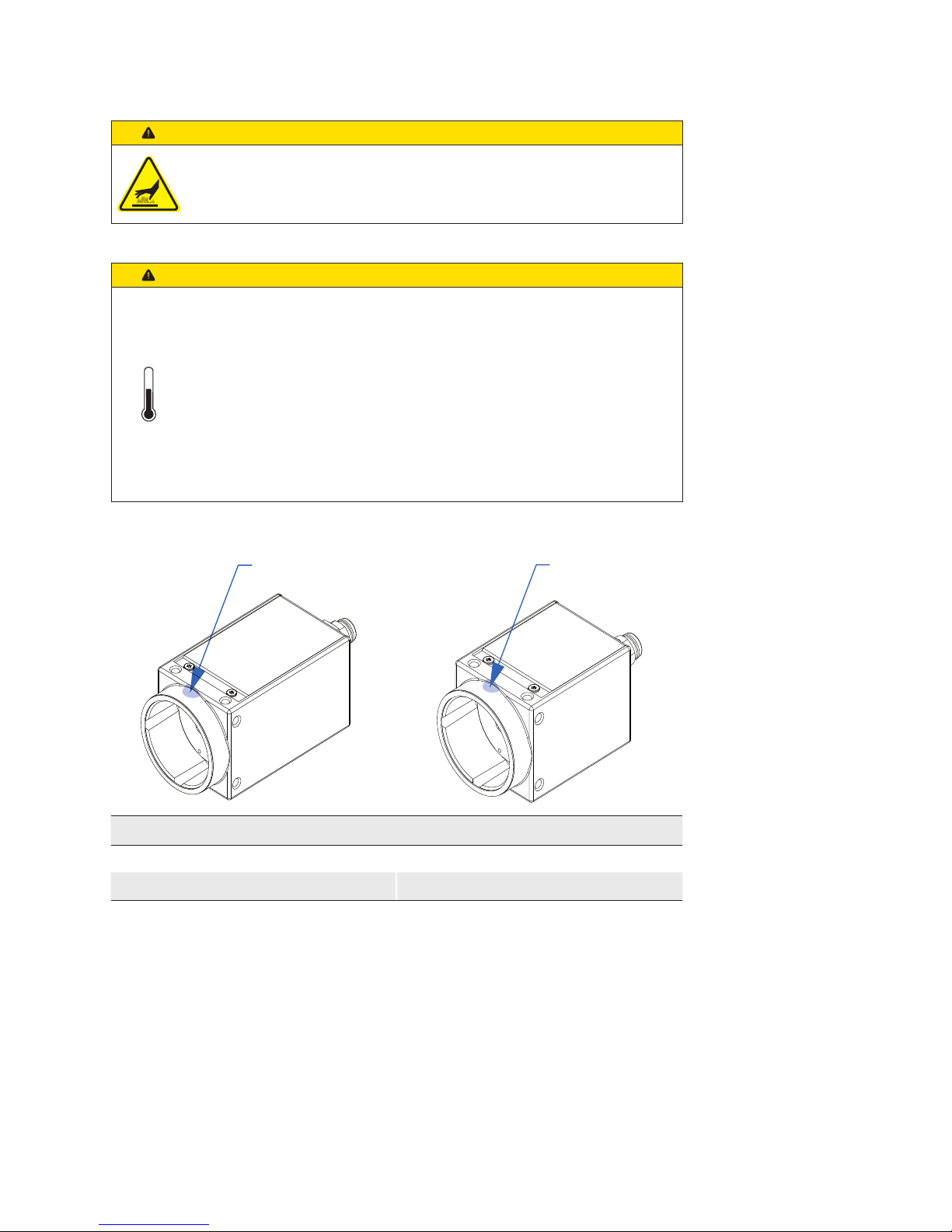
6.2 Heat Transmission
Caution
Device heats up during operation.
Skin irritation possible.
Do not touch the camera during operation.
Caution
Heat can damage the camera. Provide adequate dissipation of heat, to
ensure that the temperatures does not exceed the value (see Heat Transmission).
As there are numerous possibilities for installation, Baumer recommends
no specic method for proper heat dissipation, but suggest the following
principles:
▪ operate the cameras only in mounted condition
▪ mounting in combination with forced convection may provide proper heat
dissipation
T
T
Measure Point (T) Maximal Temperature
VCXG VCXU
65°C (149°F) 65°C (149°F)
◄Figure1
Temperature measuring
point
Page 14

14
6.3 Mechanical Tests
Environmental Testing
Standard Parameter
Vibration,
sinusodial
IEC 60068-2-6 Frequency
Range
10-2000 Hz
Amplitude underneath crossover
frequencies
1.5 mm
Acceleration 10 g
Test duration /
Axis
150 min
Vibration,
broad band
IEC 600682-64
Frequency range 20-1000 Hz
Acceleration
RMS
10 g
Test duration /
Axis
300 min
Shock IEC 60068-
2-27
Puls time 11 ms / 6 ms
Acceleration 50 g / 100 g
Bump IEC60068-2-
29
Pulse Time 2 ms
Acceleration 100 g
Page 15
15
7. Pin-Assignment / LED-Signaling
7.1 VCXG
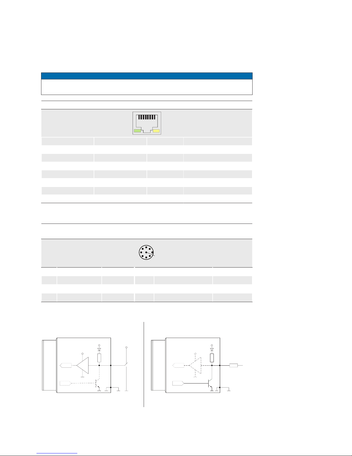
7.1.1 Ethernet Interface (PoE)
Notice
The camera supports PoE (Power over Ethernet) IEEE 802.3af Clause 33, 48V Power
supply.
8P8C Modular Jack (RJ45) with LEDs
1
8
1 green/white MX1+ (negative / positive V
port
)
2 green MX1- (negative / positive V
port
)
3 orange/white MX2+ (positive / negative V
port
)
4 blue MX3+
5 blue/white MX3-
6 orange MX2- (positive / negative V
port
)
7 brown/white MX4+
8 brown MX4-
7.1.2 Power Supply and IOs
Power Supply / Digital IOs (on camera side)
wire colors of the connecting cable (ordered separately)
8
5
7
3
1
4
2
6
1 GPIO (Line2) white
5 Power VCC OUT1
grey
2 Power V
CC
brown
6 OUT1 (Line3)
pink
3 IN1 (Line0)
green
7 GND (Power, GPIO)
blue
4 GND IN1
yellow
8 GPIO (Line1)
red
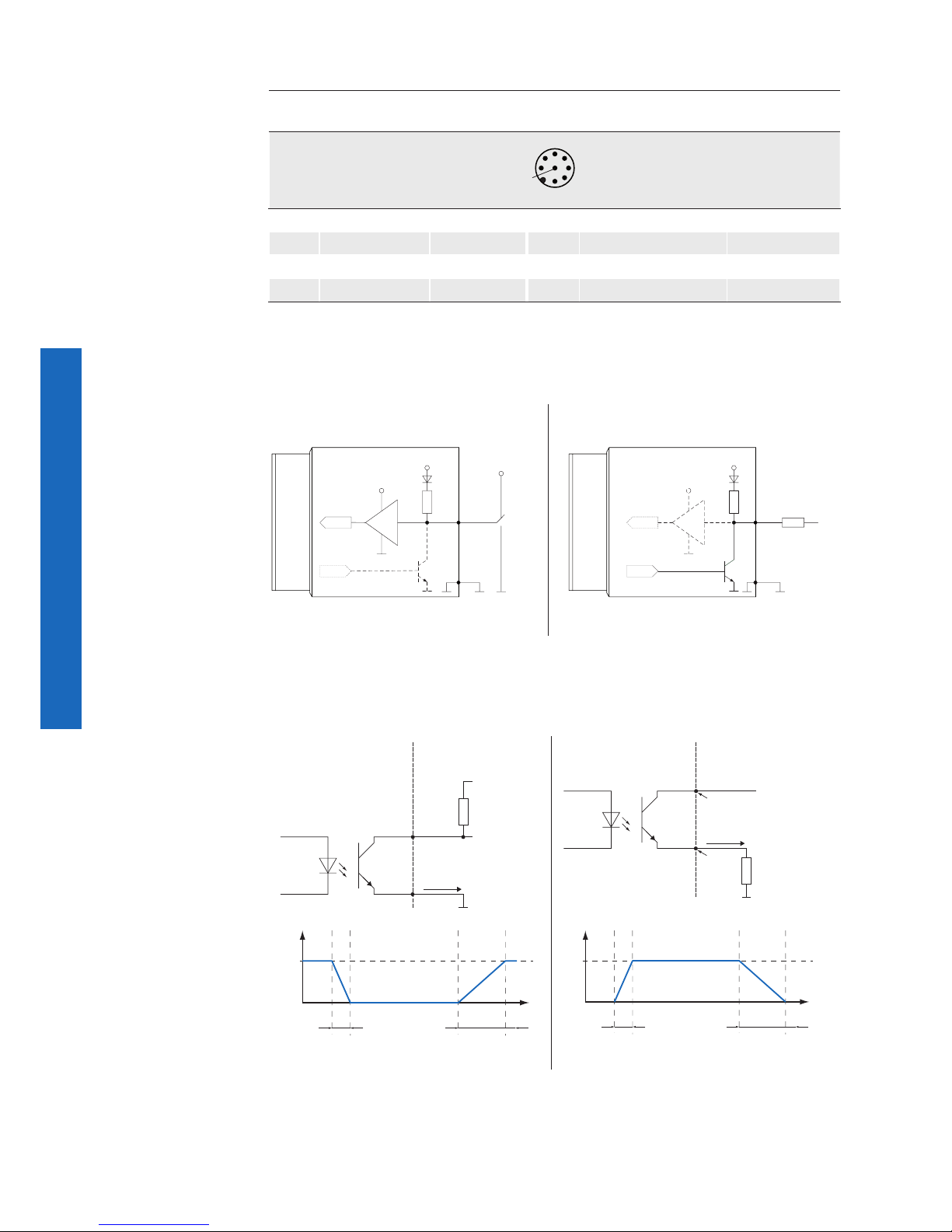
7.1.3 GPIO (General Purpose Input/Output)
Input
300
Output
Pin 1 / 8
3.3 V
3.3 V
FPGA
FPGA
FPGA
FPGA
Pin 7
Pin 1 / 8
Pin 7
Ω
300
Ω
High:
2.4 .. 3.3 V
I sink max.
= 50 mA
Low:
0 V .. 0.4 V
Low:
0 V .. 0.8 V
High:
2.0 V .. 30 V
Page 16
16
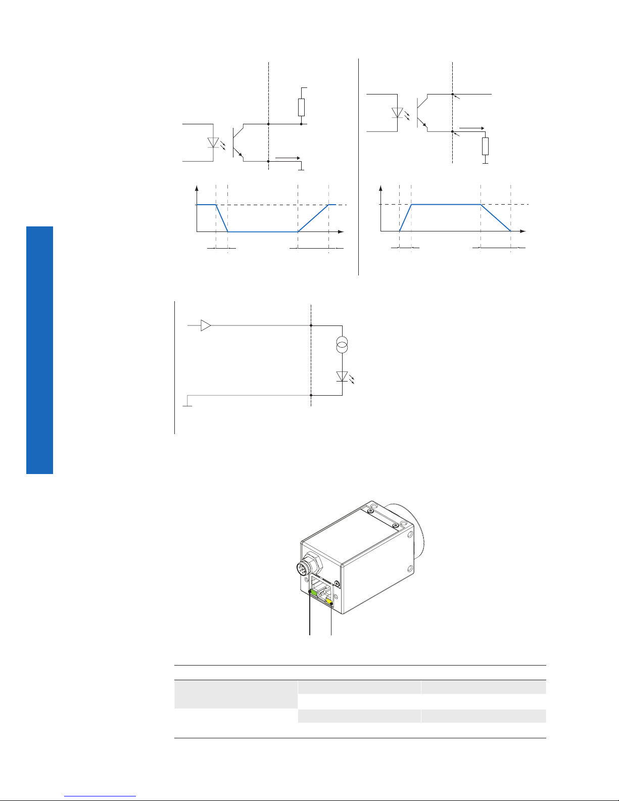
7.1.4 Digital IO
Camera Customer Device
IO Power V
CC
R
L
I
OUT
IO GND
Out
U
t
0
24V
t
OFF
t
ON
Camera Customer Device
IO Power V
CC
U
ext
Pin
R
L
I
OUT
IO GND
Out (n)
Pin
U
t
0
24V
t
ON
t
OFF
Digital Output: Low Active Digital Output: High Active
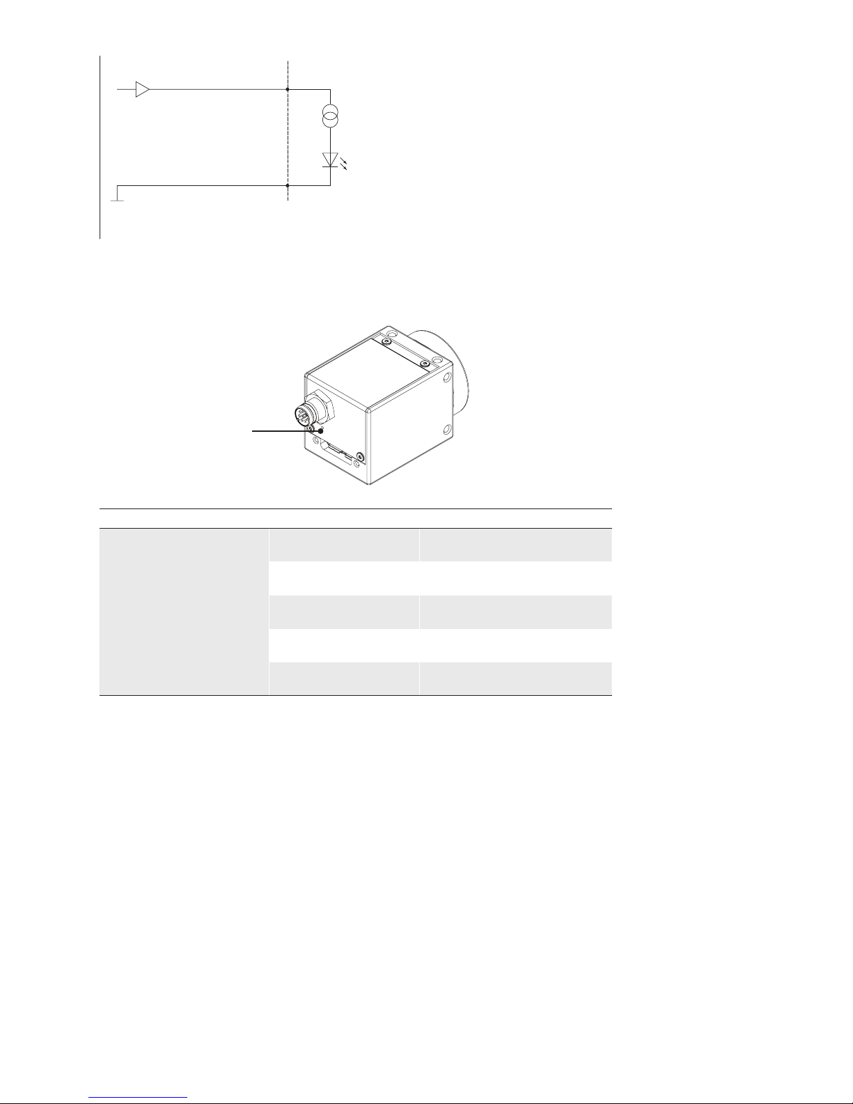
CameraCustomer Device
IO GND
DRV
Digital Input
7.1.5 LED Signaling
21
LED Signal Meaning
1
green static link active
green ash receiving
2
yellow static error
yellow ash transmitting
Figure2►
LED positions on Baumer VCXG cameras.
Page 17

17
7.2 VCXU
7.2.1 USB 3.0 Interface
USB 3.0 Micro B
12345 678910
1 VBUS 6 MicB_SSTX-
2 D- 7 MicB_SSTX+
3 D+ 8 GND_DRAIN
4 ID 9 MicB_SSRX-
5 GND 10 MicB_SSRX+
Caution
If the camera is connected to an USB2.0 port image transmission is
disabled by default. The camera consumes more than 2.5W which is the
maximum allowed by the USB2.0 specication. But there is a possibility to
activate the image transmission at your own risk!
This activation could damage your computer´s hardware!
Procedure
1. Open the camera in the Camera Explorer.
2. Select the Prole GenICam Guru.
3. Activate the Feature USB2 Support Enable in the category
Device Control.
4. Disconnect the data connection of the camera to the USB 2.0 port.
5. Connect the data connection of the camera to the USB 2.0 port.
→ Images will be transmitted via the USB 2.0 port.
Page 18
18
7.2.2 Digital IOs
Power Supply / Digital IOs (on camera side)
wire colors of the connecting cable (ordered separately)
8
5
7
3
1
4
2
6
1 GPIO (Line2) white
5 Power VCC OUT1
grey
2 not connected
brown
6 OUT1 (Line3)
pink
3 IN1 (Line0)
green
7 GND GPIO
blue
4 GND IN1
yellow
8 GPIO (Line1)
red
7.2.3 GPIO (General Purpose Input/Output)
Input
300
Output
Pin 1 / 8
3.3 V
3.3 V
FPGA
FPGA
FPGA
FPGA
Pin 7
Pin 1 / 8
Pin 7
Ω
300
Ω
High:
2.4 .. 3.3 V
I sink max.
= 50 mA
Low:
0 V .. 0.4 V
Low:
0 V .. 0.8 V
High:
2.0 V .. 30 V
7.2.4 Digital IO
Camera Customer Device
IO Power V
CC
R
L
I
OUT
IO GND
Out
U
t
0
24V
t
OFF
t
ON
Camera Customer Device
IO Power V
CC
U
ext
Pin
R
L
I
OUT
IO GND
Out (n)
Pin
U
t
0
24V
t
ON
t
OFF
Digital Output: Low Active Digital Output: High Active
Page 19
19
CameraCustomer Device
IO GND
DRV
Digital Input
7.2.5 LED Signaling
LED
Signal Meaning
LED
green ash Power on
green USB 3.0 connection
red USB 2.0 connection
yellow Readout active
red ash Update
◄Figure3
LED position on Baumer VCXU camera.
Page 20
20
8. ProductSpecications
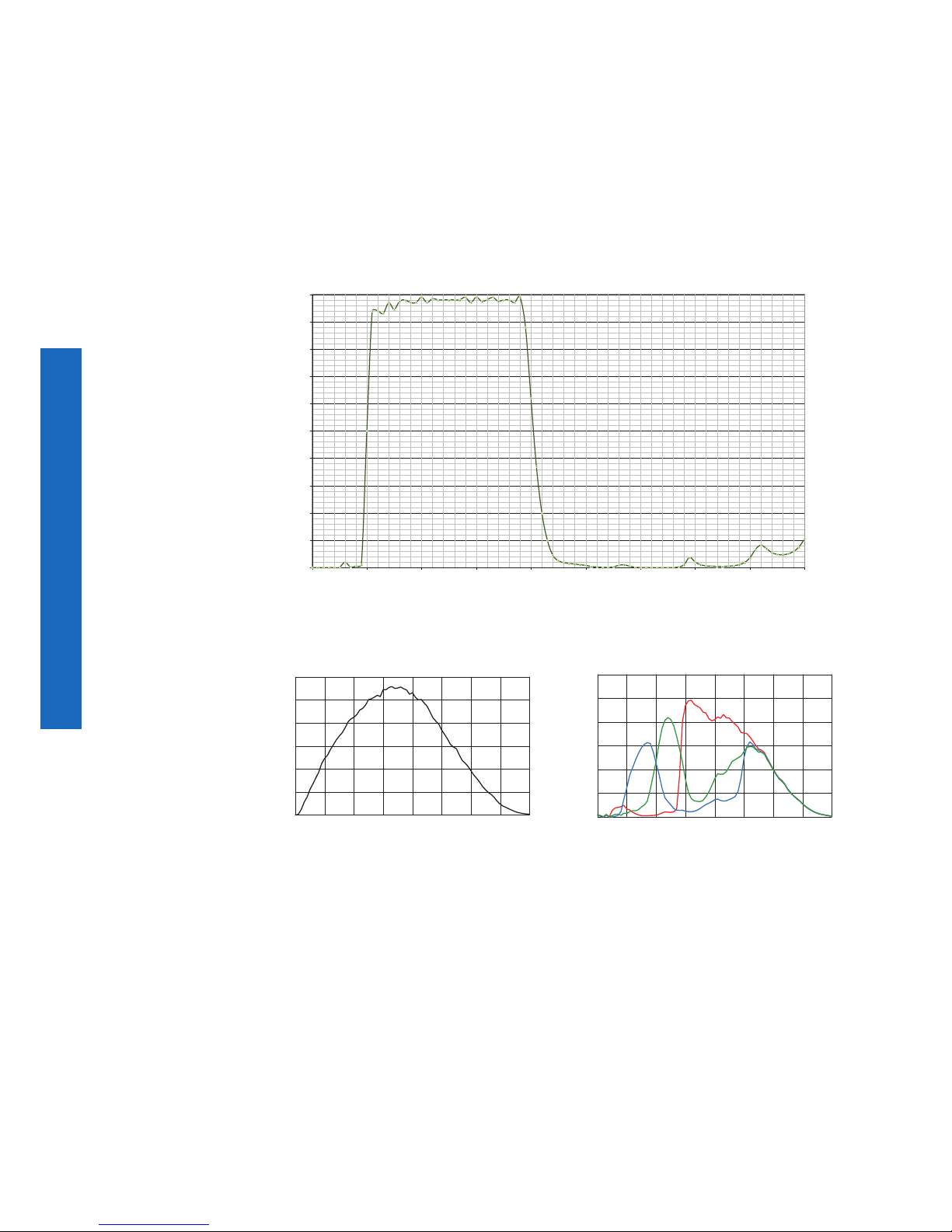
8.1 Spectral Sensitivity
The spectral sensitivity characteristics of monochrome and color matrix sensors for cameras of this series are displayed in the following graphs. The characteristic curves for
the sensors do not take the characteristics of lenses and light sources without lters into
consideration.
Values relating to the respective technical data sheets of the sensors.
0%
10%
20%
30%
40%
50%
60%
70%
80%
90%
100%
300400 500600 700800 900100011001200
Transmission
wavelength in nm
Filter glass of color cameras
Wave Length [nm]
VCXG-53M
0
1000
2000
3000
4000
5000
6000
300 400 500 600700 800900 1000
1100
Response [V/s/W/m
2
]
Wave Length [nm]
VCXG-53C
0
1000
2000
3000
4000
5000
6000
300 400 500 600700 800900 1000 1100
Response [V/s/W/m
2
]
Figure4►
Spectral sensitivities for
Baumer cameras with
5.0 MP sensor.
Page 21
21
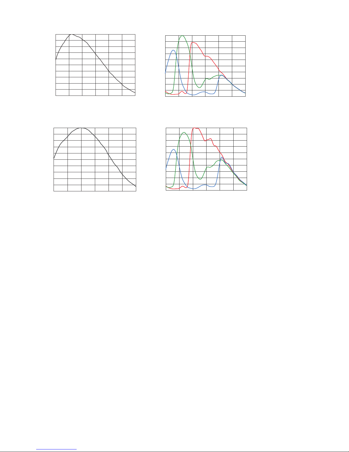
400 500 600 700 800 900 1000
0
0.2
0.4
0.6
0.8
1.0
Wave Length [nm]
Relative Response
VCXU-23M
400 500 600 700 800 900 1000
0
0.2
0.4
0.6
0.8
1.0
Wave Length [nm]
Relative Response
VCXU-23C
400 500 600 700 800 900
1000
0
0.2
0.4
0.6
0.8
1.0
Wave Length [nm]
Relative Response
VCXU-50M
400 500 600 700 800 900
1000
0
0.2
0.4
0.6
0.8
1.0
Wave Length [nm]
Relative Response
VCXU-50C
◄Figure5
Spectral sensitivities for
Baumer cameras with
2.3 MP sensor.
◄Figure6
Spectral sensitivities for
Baumer cameras with
5.0 MP sensor.
Page 22
22
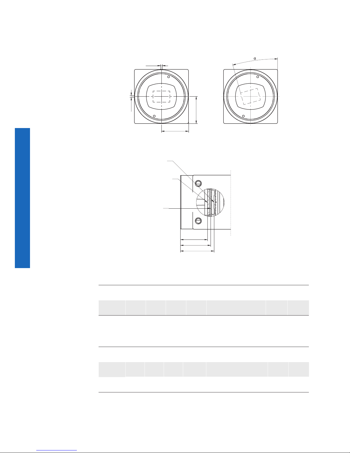
8.2 Field of View Position
The typical accuracy by assumption of the root mean square value is displayed in the
gures and the tables below:
± YM
± YR
± XR
Z
photosensitive
surface of the
sensor
front filter glass
for color cameras
thickness:
1 ± 0.1 mm
cover glass
of sensor
thickness: D
A
14,5±0,35
± XM
±
8.2.1 VCXG
Camera
Type
± xM
[mm]
± yM
[mm]
± xR
[mm]
± YR
[mm]
± z
typ
[mm]
± α
typ
[°]
A
[mm]
D**
[mm]
VCXG-
53*
0.04 0,04 0.04 0.04 17.65 ± 0.070 0.6 16.5 0.55
8.2.2 VCXU
Camera
Type
± xM
[mm]
± yM
[mm]
± xR
[mm]
± YR
[mm]
± z
typ
[mm]
± α
typ
[°]
A
[mm]
D**
[mm]
VCXU-
23*
0.04 0,04 0.04 0.04 17.63 ±
0.065 0.4 15.8 0.50
VCXU-
50*
0.11 0.11 0.11 0.11 17.63 ±
0.065 0.6 16.4 0.70
typical accuracy by assumption of the root mean square value
* C or M
** Dimension D in this table is from manufacturer datasheet
Figure7►
Sensor accuracy of the
Baumer CX series
Page 23
23
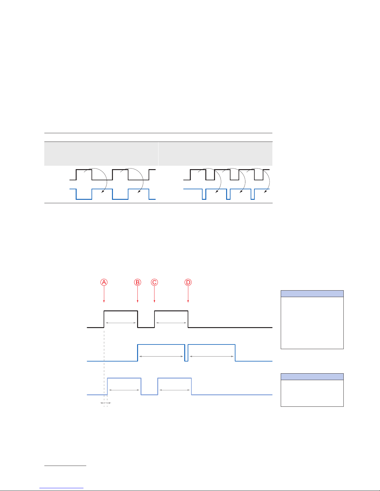
8.3 Acquisition Modes and Timings
The image acquisition consists of two separate, successively processed components.
Exposing the pixels on the photosensitive surface of the sensor is only the rst part of the
image acquisition. After completion of the rst step, the pixels are read out.
Thereby the exposure time (t
exposure
) can be adjusted by the user, however, the time need-
ed for the readout (t
readout
) is given by the particular sensor and image format.
Baumer cameras can be operated with differtent acquisition modes, the Continuous
Mode (Free Running Mode), the Acquisition Frame Rate Mode, the Single Frame Mode,
the Multi Frame Mode and the Trigger Mode.
The cameras can be operated non-overlapped
*)
or overlapped. Depending on the mode
used, and the combination of exposure and readout time:
Non-overlapped Operation Overlapped Operation
Here the time intervals are long enough
to process exposure and readout successively.
In this operation the exposure of a frame
(n+1) takes place during the readout of
frame (n).
Exposur
e
Readout
Exposur
e
Readout
8.3.1 Continuous Mode (Free Running Mode)
In the Continuous mode the camera records images permanently and sends them to the
PC. In order to achieve an optimal result (with regard to the adjusted exposure time t
exposure
and image format) the camera is operated overlapped.
In case of exposure times equal to / less than the readout time (t
exposure
≤ t
readout
), the maximum frame rate is provided for the image format used. For longer exposure times the
frame rate of the camera is reduced.
Exposure
Readout
ExposureA
ctive
t
exposure(n)
t
Exposure-
Active(n)
t
ExposureActiveDelay
t
Exposure-
Active(n+1)
t
readout(n+1)
t
readout(n)
t
exposure(n+1)
t
ExposureActive
= t
exposure
*) Non-overlapped means the same as sequential.
Image parameters:
Offset
Gain
Mode
Partial Scan
Timings:
A - exposure time
frame (n) effective
B - image parameters
frame (n) effective
C - exposure time
frame (n+1) effective
D - image parameters
frame (n+1) effective
Page 24

24
8.3.2 Single Frame Mode
In this mode the camera is captured one frame after AcquisitionStart. Then the acquisition
is stopped.
8.3.3 Multi Frame Mode
In this mode a predened number of frames will be captured after AcquisitionStart. The
AcquisitionFrameCount controls the number of captured frames. Then the acquisition is
automatically stopped.
8.3.4 Acquisition Frame Rate Mode
With this feature Baumer introduces a clever technique to the CX camera series, that
enables the user to predene a desired frame rate in continuous mode.
For the employment of this mode the cameras uses an internal clock generator that creates trigger pulses.
Notice
From a certain frame rate, skipping internal triggers is unavoidable. In general, this depends on the combination of adjusted frame rate, exposure and readout times.
Page 25

25
8.3.5 Trigger Mode
After a specied external event (trigger) has occurred, image acquisition is started. Depending on the interval of triggers used, the camera operates non-overlapped or overlapped in this mode.
With regard to timings in the trigger mode, the following basic formulas need to be taken
into consideration:
Case Formula
t
exposure
< t
readout
(1) t
earliestpossibletrigger(n+1)
= t
readout(n)
- t
exposure(n+1)
(2) t
notready(n+1)
= t
exposure(n)
+ t
readout(n)
- t
exposure(n+1)
t
exposure
> t
readout
(3) t
earliestpossibletrigger(n+1)
= t
exposure(n)
(4) t
notready(n+1)
= t
exposure(n)
8.3.5.1 Overlapped Operation: t
exposure(n+2)
= t
exposure(n+1)
In overlapped operation attention should be paid to the time interval where the camera is
unable to process occuring trigger signals (t
notready
). This interval is situated between two
exposures. When this process time t
notready
has elapsed, the camera is able to react to
external events again.
After t
notready
has elapsed, the timing of (E) depends on the readout time of the current im-
age (t
readout(n)
) and exposure time of the next image (t
exposure(n+1)
). It can be determined by the
formulas mentioned above (no. 1 or 3, as is the case).
In case of identical exposure times, t
notready
remains the same from acquisition to acquisi-
tion.
Exposure
Readout
t
exposure(n)
t
readout(n+1)
t
readout(n)
t
exposure(n+1)
t
triggerdelay
t
min
Tr
igger
ExposureA
ctive
t
Exposure-
Active(n)
t
ExposureActiveDelay
t
Exposure-
Active(n+1)
Tr
iggerReady
t
notready
Image parameters:
Offset
Gain
Mode
Partial Scan
Timings:
A - exposure time
frame (n) effective
B - image parameters
frame (n) effective
C - exposure time
frame (n+1) effective
D - image parameters
frame (n+1) effective
E - earliest possible trigger
Page 26

26
8.3.5.2 Overlapped Operation: t
exposure(n+2)
> t
exposure(n+1)
If the exposure time (t
exposure
) is increased from the current acquisition to the next acquisi-
tion, the time the camera is unable to process occurring trigger signals (t
notready
) is scaled
down.
This can be simulated with the formulas mentioned above (no. 2 or 4, as is the case).
Exposure
Readout
t
exposure(n)
t
readout(n+1)
t
readout(n)
t
exposure(n+1)
t
exposure(n+2)
t
triggerdelay
t
min
Trigger
ExposureA
ctive
t
Exposure-
Active(n)
t
ExposureActiveDelay
t
Exposure-
Active(n+1)
TriggerReady
t
notready
Image parameters:
Offset
Gain
Mode
Partial Scan
Timings:
A - exposure time
frame (n) effective
B - image parameters
frame (n) effective
C - exposure time
frame (n+1) effective
D - image parameters
frame (n+1) effective
E - earliest possible trigger
Page 27

27
8.3.5.3 Overlapped Operation: t
exposure(n+2)
< t
exposure(n+1)
If the exposure time (t
exposure
) is decreased from the current acquisition to the next acquisi-
tion, the time the camera is unable to process occurring trigger signals (t
notready
) is scaled
up.
When decreasing the t
exposure
such, that t
notready
exceeds the pause between two incoming
trigger signals, the camera is unable to process this trigger and the acquisition of the image will not start (the trigger will be skipped).
Exposure
Readout
t
exposure(n)
t
readout(n+1)
t
readout(n)
t
exposure(n+1)
t
exposure(n+2)
t
triggerdelay
t
min
Tr
igger
ExposureA
ctive
t
Exposure-
Active(n)
t
ExposureActiveDelay
t
Exposure-
Active(n+1)
Tr
iggerReady
t
notready
Notice
From a certain frequency of the trigger signal, skipping triggers is unavoidable. In general, this frequency depends on the combination of exposure and readout times.
Image parameters:
Offset
Gain
Mode
Partial Scan
Timings:
A - exposure time
frame (n) effective
B - image parameters
frame (n) effective
C - exposure time
frame (n+1) effective
D - image parameters
frame (n+1) effective
E - earliest possible trigger
F - frame not started /
trigger skipped
Page 28

28
8.3.5.4 Non-overlapped Operation
If the frequency of the trigger signal is selected for long enough, so that the image acquisitions (t
exposure
+ t
readout
) run successively, the camera operates non-overlapped.
Exposure
Readout
t
exposure(n)
t
readout(n+1)
t
readout(n)
t
exposure(n+1)
t
triggerdelay
t
min
Trigger
ExposureA
ctive
t
Exposure-
Active(n)
t
ExposureActiveDelay
t
Exposure-
Active(n+1)
TriggerReady
t
notready
Image parameters:
Offset
Gain
Mode
Partial Scan
Timings:
A - exposure time
frame (n) effective
B - image parameters
frame (n) effective
C - exposure time
frame (n+1) effective
D - image parameters
frame (n+1) effective
E - earliest possible trigger
Page 29

29
8.3.6 Advanced Timings for GigE Vision®/USB3 VisionTM Message Channel
The following events can be transmissited via the asynchronous Message Channel:
PrimaryApplicationStitch (only GigE), GigEVisionError (only GigE), GigEVisionHeartbeatTimeOut (only GigE), EventLost, Line0..3 FallingEdge, Line0..3 RisingEdge, ExposureStart, ExposureEnd, FrameStart, FrameTransferSkipped, TransferBufferFull, TriggerReady, TransferBufferReady, TriggerOverlapped, TriggerSkipped
The charts below show some timings for the event signaling by the asynchronous mes-
sage channel. Vendor-specic events are explained.
8.3.6.1 EventLost
This signal can be put out when a selected event was lost. The cause may be that too
many events occur.
8.3.6.2 TriggerReady
This event signals whether the camera is able to process incoming trigger signals or not.
Exposure
Readout
t
exposure(n)
t
readout(n+1)
t
readout(n)
t
exposure(n+1)
Tr
igger
TriggerReady
Event: TriggerReady
t
notready
8.3.6.3 TriggerSkipped
If the camera is unable to process incoming trigger signals, which means the camera
should be triggered within the interval t
notready
, these triggers are skipped. On Baumer CX
cameras the user will be informed about this fact by means of the event "TriggerSkipped".
Exposure
Readout
t
exposure(n)
t
readout(n+1)
t
readout(n)
t
exposure(n+1)
Tr
igger
Tr
iggerReady
t
notready
TriggerSkipped
Event: TriggerSkipped
Page 30

30
8.3.6.4 TriggerOverlapped
This signal is active, as long as the sensor is exposed and read out at the same time.
which means the camera is operated overlapped.
Exposure
Readout
t
exposure(n)
t
readout(n+1)
t
readout(n)
t
exposure(n+1)
Tr
igger
Tr
igger
Overlapped
Event: TriggerOverlapped
Once a valid trigger signal occures not within a readout, the "TriggerOverlapped" signal
changes to state low.
8.3.6.5 ReadoutActive
While the sensor is read out, the camera signals this by means of "ReadoutActive".
Exposure
Readout
Event: ReadoutActive
t
exposure(n)
t
readout(n+1)
t
readout(n)
t
exposure(n+1)
Tr
igger
Readout
Active
Page 31

31
8.3.6.6 TransferBufferFull
This event is issued only in trigger mode. It signals that no buffer is available.
Exposure
Readout
t
exposure(n)
t
readout(n+1)
t
readout(n)
t
exposure(n+1)
Tr
iggerReady
t
notready
BufferReady
Event: TransferBufferFull
Trigger
8.3.6.7 TransferBufferReady
This event is issued only in trigger mode. It signals that buffer available.
Exposure
Readout
Tr
ansmission
t
exposure(n)
t
readout(n+1)
t
readout(n)
t
exposure(n+1)
Tr
iggerReady
t
notready
BufferReady
Event: TransferBuff
erReady
Trigger
Page 32

32
8.4 Software
8.4.1 Baumer GAPI
Baumer GAPI stands for Baumer “Generic Application Programming Interface”. With this
API Baumer provides an interface for optimal integration and control of Baumer cameras.
This software interface allows changing to other camera models.
It provides interfaces to several programming languages, such as C, C++ and the .NET™
Framework on Windows
®
, as well as Mono on Linux® operating systems, which offers the
use of other languages, such as e.g. C# or VB.NET.
8.4.2 3rd Party Software
Strict compliance with the GenICam™ standard allows Baumer to offer the use of 3rd
Party Software for operation with cameras of this series.
You can nd a current listing of 3
rd
Party Software, which was tested successfully in com-
bination with Baumer cameras, at http://www.baumer.com/?id=2851
Page 33

33
9. Camera Functionalities
9.1 Image Acquisition
9.1.1 Image Format
A digital camera usually delivers image data in at least one format - the native resolution
of the sensor. Baumer cameras are able to provide several image formats (depending on
the type of camera).
Compared with standard cameras, the image format on Baumer cameras not only in-
cludes resolution, but a set of predened parameter.
These parameters are:
▪ Resolution (horizontal and vertical dimensions in pixels)
▪ Binning Mode
9.1.1.1 VCXG
Camera Type
Full frame
Binning 2x2
Binning 2x1
Binning 1x2
Monochrome
VCXG-53M ■ ■ ■ ■
Color
VCXG-53C ■ ■ ■ ■
9.1.1.2 VCXU
Camera Type
Full frame
Binning 2x2
Binning 2x1
Binning 1x2
Monochrome
VCXU-23M ■ ■ ■ ■
VCXU-50M ■ ■ ■ ■
Color
VCXU-23C ■ ■ ■ ■
VCXU-50C ■ ■ ■ ■
Page 34

34
9.1.2 Pixel Format
On Baumer digital cameras the pixel format depends on the selected image format.
9.1.2.1 GeneralDenitions
RAW: Raw data format. Here the data are stored without processing.
Bayer: Raw data format of color sensors.
Color lters are placed on these sensors in a checkerboard pattern, generally
in a 50% green, 25% red and 25% blue array.
Mono: Monochrome. The color range of mono images consists of shades of a single
color. In general, shades of gray or black-and-white are synonyms for monochrome.
RGB: Color model, in which all detectable colors are dened by three coordinates,
Red, Green and Blue.
Red
Gree
n
Blue
Black
White
The three coordinates are displayed within the buffer in the order R, G, B.
BGR: At BGR the interface of the camera mirrors the order of transmission of the color
channels from RGB to BGR.
This can save processing power on the computer, because these data can be
processed by the graphic card without conversion.
Figure8►
Sensor with Bayer
Pattern
Figure9►
RBG color space displayed as color cube.
Page 35

35
Pixel depth: In general, pixel depth denes the number of possible different values for
each color channel. Mostly this will be 8 bit, which means 2
8
different "col-
ors".
For RGB or BGR these 8 bits per channel equal 24 bits overall.
Two bytes are needed for transmitting more than 8 bits per pixel - even if the
second byte is not completely lled with data. In order to save bandwidth, the
packed formats were introduced to Baumer CX cameras. In this formats, the
unused bits of one pixel are lled with data from the next pixel.
8 bit:
Byte 1 Byte 2 Byte 3
12 bit:
Byte 1 Byte 2
unused bits
Packed:
Byte 1 Byte 2 Byte 3
Pixel 0Pixel 1
9.1.2.2 Pixel Formats VCXG
Camera Type
Mono8
Mono10
Mono12
Mono12p
Bayer RG8
Bayer RG10
Bayer RG12
Bayer RG12p
RGB8
BGR8
Monochrome
VCXG-53M ■ ■ □ □ □ □ □ □ □ □
Color
VCXG-53C ■ ■ □ □ ■ ■ □ □ ■ ■
9.1.2.3 Pixel Formats VCXU
Camera Type
Mono8
Mono10
Mono12
Mono12p
Bayer RG8
Bayer RG10
Bayer RG12
Bayer RG12p
RGB8
BGR8
Monochrome
VCXU-23M ■ ■ ■ ■ □ □ □ □ □ □
VCXU-50M ■ ■ ■ ■ □ □ □ □ □ □
Color
VCXU-23C □ □ □ □ ■ ■ ■ ■ □ □
VCXU-50C □ □ □ □ ■ ■ ■ ■ □ □
◄Figure10
Bit string of Mono 8 bit
and RGB 8 bit.
◄Figure11
Spreading of Mono 12
bit over two bytes.
◄Figure12
Spreading of two pixels in Mono 12 bit over
three bytes (packed
mode).
Page 36

36
9.1.3 Exposure Time
On exposure of the sensor, the inclination of photons produces a charge separation on
the semiconductors of the pixels. This results in a voltage difference, which is used for
signal extraction.
Light
Photon
Pixel
Charge Carrier
The signal strength is inuenced by the incoming amount of photons. It can be increased
by increasing the exposure time (t
exposure
).
On Baumer CX cameras, the exposure time can be set within the following ranges (step
size 1μsec):
9.1.3.1 VCXG
Camera Type t
exposure
min t
exposure
max
Monochrome
VCXG-53M 20 μsec 1 sec
Color
VCXG-53C 20 μsec 1 sec
9.1.3.2 VCXU
Camera Type t
exposure
min t
exposure
max
Monochrome
VCXU-23M 45 μsec 60 sec
VCXU-50M 45 μsec 60 sec
Color
VCXU-23C 45 μsec 60 sec
VCXU-50C 45 μsec 60 sec
Figure13►
Incidence of light
causes charge separation on the semiconductors of the sensor.
Page 37

37
9.1.4 Fixed Pattern Noise Correction (FPNC)
CMOS sensors exhibit nonuniformities that are often called xed pattern noise (FPN).
However it is no noise but a xed variation from pixel to pixel that can be corrected. The
advantage of using this correction is a more homogeneous picture which may simplify the
image analysis. Variations from pixel to pixel of the dark signal are called dark signal nonuniformity (DSNU) whereas photo response nonuniformity (PRNU) describes variations
of the sensitivity. DNSU is corrected via an offset while PRNU is corrected by a factor.
The correction is based on columns. It is important that the correction values are comput-
ed for the used sensor readout conguration. During camera production this is derived for
the factory defaults. If other settings are used (e.g. different number of readout channels)
using this correction with the default data set may degrade the image quality. In this case
the user may derive a specic data set for the used setup.
FPN Correction Off FPN Correction On
9.1.4.1 VCXG
Camera Type
FPNC
Monochrome
VCXG-53M ■
Color
VCXG-53C ■
9.1.4.2 VCXU
Camera Type
FPNC
Monochrome
VCXU-23M □
VCXU-50M □
Color
VCXU-23M □
VCXU-50C □
Page 38

38
9.1.5 Look-Up-Table
The Look-Up-Table (LUT) is employed on Baumer monochrome and color CX cameras.
It contains 212 (4096) values for the available levels. These values can be adjusted by the
user.
For color cameras the LUT is applied for all color channels together.
9.1.6 Gamma Correction
With this feature, Baumer VCX cameras offer the possibility of compensating nonlinearity
in the perception of light by the human eye.
For this correction, the corrected pixel intensity (Y') is calculated from the original intensity
of the sensor's pixel (Y
original
) and correction factor γ using the following formula (in over-
simplied version):
Y' = Y
original
γ
On Baumer VCX cameras the correction factor γ is adjustable from 0.1 to 2.
The values of the calculated intensities are entered into the Look-Up-Table. Thereby previously existing values within the LUT will be overwritten.
Notice
If the LUT feature is disabled on the software side, the gamma correction feature is
disabled, too.
H
E0
▲Figure14
Non-linear perception of
the human eye.
H - Perception of bright ness
E - Energy of light
Page 39

39
9.1.7 Region of Interest
With the "Region of Interest" (ROI) function it is possible to predene a so-called Region
of Interest (ROI) or Partial Scan. This ROI is an area of pixels of the sensor. On image
acquisition, only the information of these pixels is sent to the PC.
This function is employed, when only a region of the eld of view is of interest. It is coupled
to a reduction in resolution.
The ROI is specied by four values:
▪ Offset X - x-coordinate of the rst relevant pixel
▪ Offset Y - y-coordinate of the rst relevant pixel
▪ Size X - horizontal size of the ROI
▪ Size Y - vertical size of the ROI
9.1.7.1 ROI
Start ROI
End ROI
ROI Readout
In the illustration below, readout time would be decreased to 40%, compared to a full
frame readout.
Readout lines
◄Figure15
ROI: Parameters
◄Figure16
Decrease in readout
time by using partial
scan.
Page 40

40
9.1.8 Binning
On digital cameras, you can nd several operations for progressing sensitivity. One of
them is the so-called "Binning". Here, the charge carriers of neighboring pixels are aggregated. Thus, the progression is greatly increased by the amount of binned pixels. By
using this operation, the progression in sensitivity is coupled to a reduction in resolution.
Higher sensitivity enables shorter exposure times.
Baumer cameras support three types of Binning - vertical, horizontal and bidirectional.
In unidirectional binning, vertically or horizontally neighboring pixels are aggregated and
reported to the software as one single "superpixel".
In bidirectional binning, a square of neighboring pixels is aggregated.
Notice
Occuring deviations in brightness after binning can be corrected with Brightness
Correction function.
9.1.8.1 Monochrome Binning
Binning Illustration Output
without
1x2
2x1
2x2
Figure17►
Full frame image, no
binning of pixels.
Figure18►
Vertical binning causes
a vertically compressed
image with doubled
brightness.
Figure19►
Horizontal binning
causes a horizontally
compressed image with
doubled brightness.
Figure20►
Bidirectional binning
causes both a horizontally and vertically
compressed image with
quadruple brightness.
Page 41

41
9.1.8.2 Color Binning
Color Binning is calculating on the camera (no higher frame rates) – The sensor does not
support this binning operation.
Color calculated pixel formats
In pixel formats, which are not raw formats (e.g. RGB8), the three calculated color values
(R, G, B) of a pixel will be added with those of the corresponding neighbor pixel during
binning.
Binning Illustration
without
color calculation
1x2
color calculation
2x1
color calculation
2x2
color calculation
Binning 2x2
◄Figure21
Full frame image, no
binning of pixels.
◄Figure22
Vertical binning causes
a vertically compressed
image with doubled
brightness.
◄Figure23
Horizontal binning
causes a horizontally
compressed image with
doubled brightness.
◄Figure24
Bidirectional binning
causes both a horizontally and vertically
compressed image with
quadruple brightness.
Page 42

42
RAW pixel formats
In the raw pixel formats (e.g. BayerRG8) the color values of neighboring pixels with the
same color are combined.
Binning Illustration
without
1x2
2x1
2x2
Figure25►
Full frame image, no
binning of pixels.
Figure26►
Vertical binning causes
a vertically compressed
image with doubled
brightness.
Figure27►
Horizontal binning
causes a horizontally
compressed image with
doubled brightness.
Figure28►
Bidirectional binning
causes both a horizontally and vertically
compressed image with
quadruple brightness.
Page 43

43
9.1.9 Brightness Correction
The aggregation of charge carriers may cause an overload. To prevent this, brightness
correction was introduced. Brightness correction can be swiched on or off.
Here, three binning modes need to be considered separately:
Binninig Realization
1x2 1x2 binning is performed within the sensor, binning correction also takes
place here. A possible overload is prevented by halving the exposure time.
2x1 2x1 binning takes place within the FPGA of the camera. The binning cor-
rection is realized by aggregating the charge quantities, and then halving
this sum.
2x2 2x2 binning is a combination of the above versions.
Charge quantity
Binning 2x2
Super pixel
Total charge
quantity of the
4 aggregated
pixels
◄Figure29
Aggregation of charge
carriers from four pixels
in bidirectional binning.
Page 44

44
9.1.10 Flip Image
The Flip Image function let you ip the captured images horizontal and/or vertical before
they are transmitted from the camera.
Notice
A dened ROI will also ipped.
Notice
In the RAW image formats ipping is not possible.
Normal Flip vertical
Normal Flip horizontal
Normal Flip horizontal and vertical
Figure30►
Flip image vertical
Figure31►
Flip image horiontal
Figure32►
Flip image horiontal and
vertical
Page 45

45
9.2 Color Processing
The color cameras are balanced to a color temperature of 6500 K. With the feature Color
Transformation Factory List the color temperature can be switched between 6500 K and
3000 K.
Oversimplied, color processing is realized by 4 modules.
Camera
Module
Bayer
Processor
Color-
Transfor-
mation
RGB
r
g
b
r'
g'
b'
r''
b''
g''
White balance
The color signals r (red), g (green) and b (blue) of the sensor are amplied in total and
digitized within the camera module.
Within the Bayer processor, the raw signals r', g' and b' are amplied by using of indepen-
dent factors for each color channel. Then the missing color values are interpolated, which
results in new color values (r'', g'', b''). The luminance signal Y is also generated.
The next step is the color transformation. Here the previously generated color signals r'',
g'' and b'' are converted to optimized RGB (Color adjustment as physical balance of the
spectral sensitivities).
9.3 Color Adjustment – White Balance
This feature is available on all color cameras of the Baumer VCX series and takes place
within the Bayer processor.
White balance means independent adjustment of the three color channels, red, green and
blue by employing of a correction factor for each channel.
9.3.1 User-specicColor Adjustment
The user-specic color adjustment in Baumer color cameras facilitates adjustment of the
correction factors for each color gain. This way, the user is able to adjust the amplica-
tion of each color channel exactly to his needs. The correction factors for the color gains
range from 1 to 4.
non-adjusted
histogramm
histogramm after
user-specific
color adjustment
◄Figure33
Color processing modules of color cameras.
◄Figure34
Examples of histogramms for a nonadjusted image and for
an image after user-
specic white balance..
Page 46

46
9.3.2 One Push White Balance (Once)
Here, the three color spectrums are balanced to a single white point. The correction factors of the color gains are determined by the camera (one time).
Notice
When images are acquired in trigger mode, the white balance affects on the next acquired image.
non-adjusted
histogramm
histogramm after
„one push“ white
balance
9.3.3 Continuous White Balance
In the Continuous mode the white balance is automatically performed once per second.
9.4 Analog Controls
9.4.1 Offset / Black Level
On Baumer VCX cameras, the offset (or black level) is adjustable from 0 to 255 LSB (relating to 12 bit).
9.4.1.1 VCXG
Camera Type Step Size 1 LSB
Relating to
Monochrome
VCXG-53M 10 bit
Color
VCXG-53C 10 bit
9.4.1.2 VCXU
Camera Type Step Size 1 LSB
Relating to
Monochrome
VCXU-23M 12 bit
VCXU-50M 12 bit
Color
VCXU-23C 12 bit
VCXU-50C 12 bit
Figure35►
Examples of histogramms for a non-adjusted image and for an
image after "one push"
white balance.
Page 47

47
9.4.2 Gain
In industrial environments motion blur is unacceptable. Due to this fact exposure times
are limited. However, this causes low output signals from the camera and results in dark
images. To solve this issue, the signals can be amplied by a user-dened gain factor
within the camera. This gain factor is adjustable.
Notice
Increasing the gain factor causes an increase of image noise.
9.4.2.1 VCXG
Camera Type Gain [dB]
Monochrome
VCXG-53M 0...12
Color
VCXG-53C 0...12
9.4.2.2 VCXU
Camera Type Gain [dB]
Monochrome
VCXU-23M 0...48
VCXU-50M 0...48
Color
VCXU-23C 0...48
VCXU-50C 0...48
Page 48

48
9.5 Pixel Correction
9.5.1 General information
A certain probability for abnormal pixels - the so-called defect pixels - applies to the sensors of all manufacturers. The charge quantity on these pixels is not linear-dependent on
the exposure time.
The occurrence of these defect pixels is unavoidable and intrinsic to the manufacturing
and aging process of the sensors.
The operation of the camera is not affected by these pixels. They only appear as brighter
(warm pixel) or darker (cold pixel) spot in the recorded image.
Warm Pixel
Cold Pixel
Charge quantity
„Normal Pixel“
Charge quantity
„Cold Pixel“
Charge quantity
„Warm Pixel“
Figure36►
Distinction of "hot" and
"cold" pixels within the
recorded image.
Figure37►
Charge quantity of "hot"
and "cold" pixels compared with "normal"
pixels.
Page 49

49
9.5.2 Correction Algorithm
On Baumer cameras the problem of defect pixels is solved as follows:
▪ Possible defect pixels are identied during the production process of the camera.
▪ The coordinates of these pixels are stored in the factory settings of the camera.
▪ Once the sensor readout is completed, correction takes place:
▪ Before any other processing, the values of the neighboring pixels on the left and the
right side of the defect pixels, will be read out. (within the same bayer phase for
color)
▪ Then the average value of these 2 pixels is determined to correct the rst defect
pixel
▪ Finally, the value of the second defect pixel is is corrected by using the previously
corrected pixel and the pixel of the other side of the defect pixel.
▪ The correction is able to correct up to two neighboring defect pixels.
Defect Pixels
Average Value
Corrected Pixels
9.5.3 Defectpixellist
As stated previously, this list is determined within the production process of Baumer cameras and stored in the factory settings.
Additional hot or cold pixels can develop during the lifecycle of a camera. In this case
Baumer offers the possibility of adding their coordinates to the defectpixellist.
The user can determine the coordinates
*)
of the affected pixels and add them to the list.
Once the defect pixel list is stored in a user set, pixel correction is executed for all coordinates on the defectpixellist.
*) Position in relation to Full Frame Format (Raw Data Format / No ipping).
Page 50

50
9.6 Process Interface
9.6.1 Digital IOs
9.6.1.1 UserDenableInputs
The wiring of these input connectors is the responsibility of the user.
The sole exception to this is the compliance with predetermined high and low levels
(only the optical input IN1; 0 ... 4.5V low, 11 ... 30V high).
The dened signals will have no direct effect, but can be analyzed and processed on the
software side and used to control the camera.
Using a so called "IO matrix" allows you to select the signal and the state to be processed.
On the software side, the input signals are named "Trigger", "Timer" and "LineOut 1...3".
* Example, if the two GPIO's are used as input.
(Input) Line 1*
(Input) Line 0
(Input) Line 2*
Trigger
Timer
Events
state high
state low
IO Matrix
state selection
(inverter)
signal selection
(software side)
Figure38►
IO matrix on the input
side.
Page 51

51
9.6.1.2 General Purpose Input/Output (GPIO)
Lines 1 and 2 are GPIOs and can be inputs and outputs.
Used as an input: (0 ... .0.8 V low, 2.0 ... 30 V high).
Used as an output: (0 ... .0.4 V low, 2.4 ... 3.3 V high),
@ 1 mA load (high) / 50 mA sink (low)
Caution
The General Purpose IOs (GPIOs) are not potential-free and do not have an
overrun cut-off. Incorrect wiring (overvoltage, undervoltage or voltage reversal) can lead to defects within the electronics system.
GPIO Power V
CC
: 3.3 V DC
Load resistor for TTL-High-Level: approx. 2.7 kΩ
The GPIOs are congured as an input through the default camera settings.
They must be connected to GPIO_GND if not used or not congured as an
output.
Input
300
Output
Pin 1 / 8
3.3 V
3.3 V
FPGA
FPGA
FPGA
FPGA
Pin 7
Pin 1 / 8
Pin 7
Ω
300
Ω
High:
2.4 .. 3.3 V
I sink max.
= 50 mA
Low:
0 V .. 0.4 V
Low:
0 V .. 0.8 V
High:
2.0 V .. 30 V
Page 52

52
9.6.1.3 CongurableOutputs
With this feature, Baumer gives you the option to wire the output connectors to internal
signals that are controlled on the software side.
On CX cameras, the output connector can be wired to one of the provided internal signals:
Signals
Off UserOutput1
TriggerReady Timer1
ExposureActive ReadoutActive
(Output) Line 0
state high
state low
(Output) Line 1*
state high
state low
(Output) Line 2*
state high
state low
IO Matrix
state selection
(inverter)
signal selection
(software side)
Signals
* Example, if the two GPIO's are used as Output.
Figure39►
IO matrix
Page 53

53
9.6.2 Trigger
Trigger signals are used to synchronize the camera exposure and a machine cycle or, in
case of a software trigger, to take images at predened time intervals.
Trigger (valid)
Exposure
Readout
Time
A
B
C
Different trigger sources can be used here.
9.6.3 Trigger Source
p
h
o
t
o
e
l
e
c
t
r
i
c
s
e
n
s
o
r
t
r
i
g
g
e
r
s
i
g
n
a
l
p
r
o
g
r
a
m
m
a
b
l
e
l
o
g
i
c
c
o
n
t
r
o
l
l
e
r
o
t
h
e
r
s
s
o
f
t
w
a
r
e
t
r
i
g
g
e
r
H
a
r
d
w
a
r
e
t
r
i
g
g
e
r
b
r
o
a
d
c
a
s
t
(
C
X
G
o
n
l
y
)
VCXU
VCXG
Each trigger source has to be activated separately. When the trigger mode is activated,
the hardware trigger is activated by default.
▲Figure40
Trigger signal, valid for
Baumer cameras.
high
low
U
t0
4.5V
11V
30V
◄Figure41
Camera in trigger
mode:
A - Trigger delay
B - Exposure time
C - Readout time
Trigger Delay:
The trigger delay is a
exible user-dened delay
between the given trigger
impulse and the image capture. The delay time can
be set between 0.0 μsec
and 2.0 sec with a stepsize
of 1 μsec. In the case of
multiple triggers during the
delay the triggers will be
stored and delayed, too.
The buffer is able to store
up to 512 trigger
signals during the delay.
Your benets:
▪ No need for a perfect
alignment of an external
trigger sensor
▪ Different objects can be
captured without hardware
changes
◄Figure42
Examples of possible
trigger sources.
Page 54

54
9.6.4 Debouncer
The basic idea behind this feature was to seperate interfering signals (short peaks) from
valid square wave signals, which can be important in industrial environments. Debouncing
means that invalid signals are ltered out, and signals lasting longer than a user-dened
testing time t
DebounceHigh
will be recognized, and routed to the camera to induce a trigger.
In order to detect the end of a valid signal and lter out possible jitters within the signal, a
second testing time t
DebounceLow
was introduced. This timing is also adjustable by the user.
If the signal value falls to state low and does not rise within t
DebounceLow
, this is recognized
as end of the signal.
The debouncing times t
DebounceHigh
and t
DebounceLow
are adjustable from 0 to 5 msec in steps
of 1 μsec.
low
high
U
t0
4.5V
11V
30V
low
high
U
t0
4.5V
11V
30V
t
∆t
1
∆tx - high time of the signal
t
DebounceHigh
- user-defined debouncer delay for state high
t
DebounceLow
- user-defined debouncer delay for state low
t
DebounceHigh
∆t
2
∆t
3
∆t4∆t
5
∆t
6
t
DebounceLow
Incoming signals
(valid and invalid)
Debouncer
Filtered signal
9.6.5 ExposureActive (Flash Signal)
This signal is managed by exposure of the sensor.
Furthermore, the falling edge of the ExposureActive signal can be used to trigger a movement of the inspected objects. Due to this fact, the span time used for the sensor readout
t
readout
can be used optimally in industrial environments.
Debouncer:
Please note that the edges
of valid trigger signals are
shifted by t
DebounceHigh
and
t
DebounceLow
!
Depending on these
two timings, the trigger
signal might be temporally
stretched or compressed.
Page 55

55
9.6.6 Timers
Timers were introduced for advanced control of internal camera signals.
For example the employment of a timer allows you to control the ash signal in that way,
that the illumination does not start synchronized to the sensor exposure but a predened
interval earlier.
On Baumer VCX cameras the timer conguration includes four components:
Exposur
e
Timer
t
exposure
t
triggerdelay
Tr
igger
t
TimerDuration
t
TimerDelay
Component Description
TimerTriggerSource This feature provides a source selection for each timer.
TimerTriggerActivation This feature selects that part of the trigger signal (edges or
states) that activates the timer.
TimerDelay This feature represents the interval between incoming trigger
signal and the start of the timer.
TimerDuration By this feature the activation time of the timer is adjustable.
9.6.6.1 ExposureActiveDelay
As previously stated, the Timer feature can be used to start the connected illumination
earlier than the sensor exposure.
This implies a timer conguration as follows:
▪ The ash output needs to be wired to the selected internal Timer signal.
▪ Trigger source and trigger activation for the Timer need to be the same as for the
sensor exposure.
▪ The TimerDelay feature (t
TimerDelay
) needs to be set to a lower value than the trigger
delay (t
triggerdelay
).
▪ The duration (t
TimerDuration
) of the timer signal should last until the exposure of the sensor
is completed. This can be realized by using the following formula:
t
TimerDuration
= (t
triggerdelay
– t
TimerDelay
) + t
exposure
9.6.7 Frame Counter
The frame counter is part of the Baumer image infoheader and supplied with every image,
if the chunkmode is activated. It is generated by hardware and can be used to verify that
every image of the camera is transmitted to the PC and received in the right order.
◄Figure43
Possible Timer conguration
Page 56

56
9.7 Device Reset
The feature Device Reset corresponds to the turn off and turn on of the camera. This is
necessary after a parameterization (e.g. the network data) of the camera.
The interrupt of the power supply ist therefore no longer necessary.
9.8 User Sets
Four user sets (0-3) are available for the Baumer cameras of the VCX series. User set 0
is the default set and contains the factory settings. User sets 1 to 3 are user-specic and
can contain any user denable parameters.
These user sets are stored within the camera and can be loaded, saved and transferred
to other cameras of the VCX series.
By employing a so-called "user set default selector", one of the four possible user sets
can be selected as default, which means, the camera starts up with these adjusted parameters.
9.8.1 VCXG
Parameter
AcquisitionMode LineDebouncerHighTimeAbs
AcquisitionFrameCount LineDebouncerLowTimeAbs
AcquisitionStart Width
AcquisitionStop Height
AcquisitionFrameRate OffsetX
TriggerMode OffsetY
TriggerSource BinningHorizontal
TriggerActivation BinningVertical
TriggerDelay ReverseX
BalanceWhiteAuto ReverseY
ExposureTime PixelFormat
AcquisitionFrameRateEnable TestPatternGeneratorSelector
ReadoutMode TestPattern
Gain LUTEnable
Gamma LUTValue
BlackLevel DefectPixelCorrection
BrightnessCorrection ActionDeviceKey
ChunkModeActive ActionGroupMask
ChunkEnable ActionGroupKey
TimerDuration GEV SCPD
TimerDelay GEV SCFTD
TimerTriggerSource FixedPatternNoiseCorrection
TimerTriggerActivation DeviceLinkThroughputLimit
FrameCounter EventNotication
LineInverter
LineSource
UserOutputValue
UserOutputValueAll
Page 57

57
9.8.2 VCXU
Parameter
AcquisitionMode LineInverter
AcquisitionFrameCount LineSource
AcquisitionStart UserOutputValue
AcquisitionStop UserOutputValueAll
AcquisitionAbort LineDebouncerHighTimeAbs
AcquisitionFrameRate LineDebouncerLowTimeAbs
TriggerMode EventNotication
TriggerSource Width
TriggerActivation Height
TriggerDelay OffsetX
ExposureMode OffsetY
ExposureTime BinningHorizontal
AcquisitionFrameRateEnable BinningVertical
ReadoutMode ReverseX
Gain ReverseY
Gamma PixelFormat
BalanceWhiteAuto TestPatternGeneratorSelector
BlackLevel TestPattern
BrightnessCorrection LUTEnable
ChunkModeActive LUTValue
ChunkEnable DefectPixelCorrection
TimerDuration DeviceLinkThroughputLimit
TimerDelay
TimerTriggerSource
TimerTriggerActivation
FrameCounter
9.9 Factory Settings
The factory settings are stored in "user set 0" which is the default user set. This is the only
user set, that is not editable.
Page 58

58
9.10 Timestamp
The Timestamp is 64 bits long and reports the current value of the device timestamp
counter in nanoseconds. Any image or event includes its corresponding timestamp.
The resolution is at USB cameras 10 nanoseconds and at GigE cameras 8 nanoseconds.
At power on or reset (only GigE), the timestamp starts running from zero.
1122354
1122454
1122554
1122754
1123154
1123354
1122654
1123054
1123254
Figure44►
Timestamps of recorded images.
Page 59

59
9.11 Chunk
The chunk is a data packet that is generated by the camera and integrated into the payload (every image), if chunk mode is activated.
This integrated data packet can contains adjustable settings for the image.
Feature Description
ChunkOffsetX Horizontal offset from the origin to the area of interest
(in pixels).
ChunkOffsetY Vertical offset from the origin to the area of interest
(in pixels).
ChunkWidth Returns the width of the image included in the pay-
load.
ChunkHeight Returns the height of the image included in the pay-
load.
ChunkPixelFormat Returns the pixel format of the image included in the
payload.
ChunkBinningHorizontal Number of horizontal photo-sensitive cells to combine
together.
ChunkBinningVertical Number of vertical photo-sensitive cells to combine
together.
ChunkImageControl (subordinate features only together selectable)
ChunkBrightnessCorrection On/Off for the Brightness Correction.
ChunkDefectPixelCorrection On/Off the correction of defect pixels.
ChunkLUTSelector Selects the Chunk LUT.
ChunkLUTEnable On/Off the selected LUT.
ChunkReverseX On/Off Flip horizontally the image sent by the device.
The Region of interest is applied after the ipping
ChunkReverseY On/Off Flip vertically the image sent by the device.
The Region of interest is applied after the ipping.
ChunkExposureTime Returns the exposure time used to capture the im-
age.
ChunkBlackLevel Returns the black level used to capture the image in-
cluded in the payload.
ChunkGainSelector Selects which Gain to retrieve data from.
ChunkGain Returns the gain used to capture the image.
ChunkFrameID Returns the unique Identier of the frame (or image)
included in the payload.
ChunkTimestamp Returns the Timestamp of the image included in the
payload at the time of the FrameStart internal event.
ChunkDeviceTemperature Device temperature in degrees Celsius (C). It is mea-
sured at the location selected by DeviceTemperatureSelector.
ChunkLineStatusAll Returns the current status of all available Line signals
at time of polling in a single biteld.
◄Figure45
Location of the Chunk
Page 60

60
10. VCXG - Interface Functionalities
10.1 Device Information
This Gigabit Ethernet-specic information on the device is part of the Discovery-Acknowl-
edge of the camera.
Included information:
▪ MAC address
▪ Current IP conguration (persistent IP / DHCP / LLA)
▪ Current IP parameters (IP address, subnet mask, gateway)
▪ Manufacturer's name
▪ Manufacturer-specic information
▪ Device version
▪ Serial number
▪ User-dened name (user programmable string)
10.2 Packet Size and Maximum Transmission Unit (MTU)
Network packets can be of different sizes. The size depends on the network components
employed. When using GigE Vision® compliant devices, it is generally recommended to
use larger packets. On the one hand the overhead per packet is smaller, on the other
hand larger packets cause less CPU load.
The packet size of UDP packets can differ from 576 Bytes up to the MTU.
The MTU describes the maximal packet size which can be handled by all network components involved.
In principle modern network hardware supports a packet size of 1500 Byte, which is
specied in the GigE network standard. "Jumboframes" merely characterizes a packet
size exceeding 1500 Bytes.
Baumer VCXG cameras can handle a MTU of up to 16384 Bytes.
10.3 Inter Packet Gap (IPG)
To achieve optimal results in image transfer, several Ethernet-specic factors need to be
considered when using Baumer VCX cameras.
Upon starting the image transfer of a camera, the data packets are transferred at maximum transfer speed (1 Gbit/sec). In accordance with the network standard, Baumer employs a minimal separation of 12 Bytes between two packets. This separation is called
"inter packet gap" (IPG). In addition to the minimal IPG, the GigE Vision
®
standard stipu-
lates that the IPG be scalable (user-dened).
Notice
According to the Ethernet standard, IPG
min
can not be lower than 12 Bytes.
IPG:
The IPG is measured in
ticks.
An easy rule of thumb is:
1 Tick is equivalent to 1 Bit
of data.
You should also not forget
to add the various ethernet
headers to your calculation.
Page 61

61
10.3.1 Example 1: Multi Camera Operation – Minimal IPG
Setting the IPG to minimum means every image is transfered at maximum speed. Even
by using a frame rate of 1 fps this results in full load on the network. Such "bursts" can
lead to an overload of several network components and a loss of packets. This can occur,
especially when using several cameras.
In the case of two cameras sending images at the same time, this would theoretically occur at a transfer rate of 2 Gbits/sec. The switch has to buffer this data and transfer it at a
speed of 1 Gbit/sec afterwards. Depending on the internal buffer of the switch, this oper-
ates without any problems up to n cameras (n ≥ 1). More cameras would lead to a loss of
packets. These lost packets can however be saved by employing an appropriate resend
mechanism, but this leads to additional load on the network components.
10.3.2 Example 2: Multi Camera Operation – Optimal IPG
A better method is to increase the IPG to a size of
optimal IPG = (number of cameras-1)*packet size + 2 × minimal IPG
In this way both data packets can be transferred successively (zipper principle), and the
switch does not need to buffer the packets.
▲Figure46
Operation of two cameras employing a Gigabit
Ethernet switch.
Data processing within
the switch is displayed
in the next two gures.
◄Figure47
Operation of two cameras employing aminimal inter packet
gap (IPG).
◄Figure48
Operation of two cameras employing an optimal
inter packet gap (IPG).
Max. IPG:
On the Gigabit Ethernet
the max. IPG and the data
packet must not exceed 1
Gbit. Otherwise data packets can be lost.
Page 62

62
10.4 Transmission Delay
Another approach for packet sorting in multi-camera operation is the so-called Transmission Delay.
Due to the fact, that the currently recorded image is stored within the camera and its
transmission starts with a predened delay, complete images can be transmitted to the
PC at once.
The following gure should serve as an example:
For the image processing three cameras are employed – for example camera 1: VXCG53M, camera 2: VXCG-53M, camera 3: VXCG-53M.
Due to process-related circumstances, the image acquisitions of all cameras end at the
same time. Now the cameras are not trying to transmit their images simultaniously, but –
according to the specied transmission delays – subsequently. Thereby the rst camera
starts the transmission immediately – with a transmission delay "0".
10.4.1 Time Saving in Multi-Camera Operation
As previously stated, the transmission delay feature was especially designed for multi-
camera operation with employment of different camera models. Just here an signicant
acceleration of the image transmission can be achieved:
For the above mentioned example, the employment of the transmission delay feature
results in a time saving – compared to the approach of using the inter packet gap – of approx. 45% (applied to the transmission of all three images).
Figure49►
Principle of the transmission delay.
Figure50►
Comparison of transmission
delay and inter packet gap,
employed for a multi-camera
system with different camera
models.
Page 63

63
10.4.2 CongurationExample
For the three employed cameras the following data are known:
Camera
Model
Sensor
Resolution
[Pixel]
Pixel Format
(Pixel Depth)
[bit]
Resulting
Data Volume
[bit]
Readout
Time
[msec]
Exposure
Time
[msec]
Transfer
Time (GigE)
[msec]
VCXG-53M 2592 x 2048 8 42467328 35.3 20 ≈ 39.55
VCXG-53M 2592 x 2048 8 42318976 35.3 20 ≈ 39.55
VCXG-53M 2592 x 2048 8 42318976 35.3 20 ≈ 39.55
▪ The sensor resolution and the readout time (t
readout
) can be found in the respective
Technical Data Sheet (TDS). For the example a full frame resolution is used.
▪ The exposure time (t
exposure
) is manually set to 35.3 msec.
▪ The resulting data volume is calculated as follows:
Resulting Data Volume = horizontal Pixels × vertical Pixels × Pixel Depth
▪ The transfer time (t
transferGigE
) for full GigE transfer rate is calculated as follows:
Transfer Time (GigE) = Resulting Data Volume / 10243 × 1000 [msec]
All the cameras are triggered simultaneously.
The transmission delay is realized as a counter, that is started immediately after the sensor readout is started.
Camera 1
(TXG13)
Trigger
Camera 2
(TXG06)
Camera 3
(TXG03)
t
exposure(Camera 1)
t
exposure(Camera 2)
t
exposure(Camera 3)
t
readout(Camera 3)
t
transferGigE(Camera 3)
t
readout(Camera 2)
t
transferGigE(Camera 2)
t
readout(Camera 1)
t
transfer(Camera 1)*
TransmissionDelay
Camera 2
TransmissionDelay
Camera 3
Timings:
A - exposure start for all
cameras
B - all cameras ready for
transmission
C - transmission start
camera 2
D - transmission start
camera 3
* Due to technical issues
the data transfer of
camera 1 does not take
place with full GigE
speed.
◄Figure51
Timing diagram for the
transmission delay of
the three employed
cameras, using even
exposure times.
Page 64

64
In general, the transmission delay is calculated as:
∑
≥
−
+−+=
n
3n
)1nCamera(gEtransferGi)nCamera(osureexp)1Came ra(readout)1Camera(osureexp)nCamera(onDelayTransmissi
ttttt
Therewith for the example, the transmission delays of camera 2 and 3 are calculated as
follows:
t
TransmissionDelay(Camera 2)
= t
exposure(Camera 1)
+ t
readout(Camera 1)
- t
exposure(Camera 2)
t
TransmissionDelay(Camera 3)
= t
exposure(Camera 1)
+ t
readout(Camera 1)
- t
exposure(Camera 3)
+ t
transferGige(Camera 2)
Solving this equations leads to:
t
TransmissionDelay(Camera 2)
= 20 msec + 35.3 msec - 20 msec
= 35.3 msec
= 35300000 ticks
t
TransmissionDelay(Camera 3)
= 20 msec + 35.3 msec - 20 msec + 39.55 msec
= 74,85 msec
= 74850000 ticks
Notice
In Baumer GAPI the delay is specied in ticks. How do convert microseconds into ticks?
1 tick = 1 ns
1 msec = 1000000 ns
1 tick = 0,000001 msec
ticks= t
TransmissionDelay
[msec] / 0.000001 = t
TransmissionDelay
[ticks]
Page 65

65
10.5 Multicast
Multicasting offers the possibility to send data packets to more than one destination address – without multiplying bandwidth between camera and Multicast device (e.g. Router
or Switch).
The data is sent out to an intelligent network node, an IGMP (Internet Group Management
Protocol) capable Switch or Router and distributed to the receiver group with the specic
address range.
In the example on the gure below, multicast is used to process image and message data
separately on two differents PC's.
Multicast Addresses:
For multicasting Baumer
suggests an adress
range from 232.0.1.0 to
232.255.255.255.
◄Figure52
Principle of Multicast
Page 66

66
10.6 IPConguration
10.6.1 Persistent IP
A persistent IP adress is assigned permanently. Its validity is unlimited.
Notice
Please ensure a valid combination of IP address and subnet mask.
IP range: Subnet mask:
0.0.0.0 – 127.255.255.255 255.0.0.0
128.0.0.0 – 191.255.255.255 255.255.0.0
192.0.0.0 – 223.255.255.255 255.255.255.0
These combinations are not checked by Baumer GAPI, Baumer GAPI Viewer or camera
on the y. This check is performed when restarting the camera, in case of an invalid
IP - subnet combination the camera will start in LLA mode.
* This feature is disabled by default.
10.6.2 DHCP(DynamicHostCongurationProtocol)
The DHCP automates the assignment of network parameters such as IP addresses, subnet masks and gateways. This process takes up to 12 sec.
Once the device (client) is connected to a DHCP-enabled network, four steps are processed:
▪ DHCP Discovery
In order to nd a DHCP server, the client sends a so called DHCPDISCOVER broadcast to the network.
▪ DHCP Offer
After reception of this broadcast, the DHCP server will answer the request by an
unicast, known as DHCPOFFER. This message contains several items of information,
such as:
Information for the client
MAC address
offered IP address
Information on server
IP adress
subnet mask
duration of the lease
Internet Protocol:
On Baumer cameras IP v4
is employed.
Figure53▲
Connection pathway for
Baumer Gigabit Ethernet cameras:
The device connects
step by step via the
three described mechanisms.
DHCP:
Please pay attention to the
DHCP Lease Time.
Figure54►
DHCP Discovery
(broadcast)
Figure61►
DHCP offer (unicast)
Page 67

67
▪ DHCP Request
Once the client has received this DHCPOFFER, the transaction needs to be con-
rmed. For this purpose the client sends a so called DHCPREQUEST broadcast to the
network. This message contains the IP address of the offering DHCP server and
informs all other possible DHCPservers that the client has obtained all the necessary
information, and there is therefore no need to issue IP information to the client.
▪ DHCP Acknowledgement
Once the DHCP server obtains the DHCPREQUEST, an unicast containing all neces-
sary information is sent to the client. This message is called DHCPACK.
According to this information, the client will congure its IP parameters and the process is complete.
10.6.3 LLA
LLA (Link-Local Address) refers to a local IP range from 169.254.0.1 to 169.254.254.254
and is used for the automated assignment of an IP address to a device when no other
method for IP assignment is available.
The IP address is determined by the host, using a pseudo-random number generator,
which operates in the IP range mentioned above.
Once an address is chosen, this is sent together with an ARP (Address Resolution Protocol) query to the network to to check if it already exists. Depending on the response,
the IP address will be assigned to the device (if not existing) or the process is repeated.
This method may take some time - the GigE Vision
®
standard stipulates that establishing
connection in the LLA should not take longer than 40 seconds, in the worst case it can
take up to several minutes.
10.6.4 Force IP
*)
Inadvertent faulty operation may result in connection errors between the PC and the camera.
In this case "Force IP" may be the last resort. The Force IP mechanism sends an IP address and a subnet mask to the MAC address of the camera. These settings are sent
without verication and are adapted immediately by the client. They remain valid until the
camera is de-energized.
*) In the GigE Vision® standard, this feature is dened as "Static IP".
◄Figure55
DHCP Request
(broadcast)
◄Figure56
DHCP Acknowledgement (unicast)
DHCP Lease Time:
The validity of DHCP IP
addresses is limited by the
lease time. When this time
is elapsed, the IP conguration needs to be redone.
This causes a connection
abort.
LLA:
Please ensure operation
of the PC within the same
subnet as the camera.
Page 68

68
10.7 Packet Resend
Due to the fact, that the GigE Vision® standard stipulates using a UDP - a stateless user
datagram protocol - for data transfer, a mechanism for saving the "lost" data needs to be
employed.
Here, a resend request is initiated if one or more packets are damaged during transfer
and - due to an incorrect checksum - rejected afterwards.
On this topic one must distinguish between three cases:
10.7.1 Normal Case
In the case of unproblematic data transfer, all packets are transferred in their correct order
from the camera to the PC. The probability of this happening is more then 99%.
10.7.2 Fault 1: Lost Packet within Data Stream
If one or more packets are lost within the data stream, this is detected by the fact, that
packet number n is not followed by packet number (n+1). In this case the application
sends a resend request (A). Following this request, the camera sends the next packet and
then resends (B) the lost packet.
In our example packet no. 3 is lost. This fault is detected on packet no. 4, and the resend request triggered. Then the camera sends packet no. 5, followed by resending
packet no. 3.
10.7.3 Fault 2: Lost Packet at the End of the Data Stream
In case of a fault at the end of the data stream, the application will wait for incoming pack-
ets for a predened time. When this time has elapsed, the resend request is triggered and
the "lost" packets will be resent.
Figure57►
Data stream without
damaged or lost packets.
Figure58►
Resending lost packets
within the data stream.
Page 69

69
In our example, packets from no. 3 to no. 5 are lost. This fault is detected after the
predened time has elapsed and the resend request (A) is triggered. The camera then
resends packets no. 3 to no. 5 (B) to complete the image transfer.
10.7.4 Termination Conditions
The resend mechanism will continue until:
▪ all packets have reached the pc
▪ the maximum of resend repetitions is reached
▪ the resend timeout has occured or
▪ the camera returns an error.
◄Figure59
Resending of lost packets at the end of the
data stream.
Page 70

70
10.8 Message Channel
The asynchronous message channel is described in the GigE Vision® standard and offers the possibility of event signaling. There is a timestamp (64 bits) for each announced
event, which contains the accurate time the event occurred.
Each event can be activated and deactivated separately.
10.8.1 Event Generation
Event Description
GenICam™
ExposureStart Exposure started
ExposureEnd Exposure ended
FrameStart Acquisition of a frame started
FrameEnd Acquisition of a frame ended
Line0Rising Rising edge detected on IO-Line 0
Line0Falling Falling edge detected on IO-Line 0
Line1Rising Rising edge detected on IO-Line 1
Line1Falling Falling edge detected on IO-Line 1
Line2Rising Rising edge detected on IO-Line 2
Line2Falling Falling edge detected on IO-Line 2
Line3Rising Rising edge detected on IO-Line 3
Line3Falling Falling edge detected on IO-Line 3
Vendor-specic
EventError Error in event handling
EventLost Occured event not analyzed
TriggerReady t
notready
elapsed, camera is able to
process incoming trigger
TriggerOverlapped Overlapped Mode detected
TriggerSkipped Camera overtriggered
FrameTransferSkipped Frame lost in the camera
TransferBufferFull No free buffer in camera memory
TransferBufferReady Buffer availabe in camera memory
HeartBeatTimeout The device runs in heartbeat timeout
PrimaryApplicationSwitch A primary application switchover has been granted
Page 71

71
10.9 Action Command / Trigger over Ethernet
The basic idea behind this feature was to achieve a simultaneous trigger for multiple
cameras.
Therefore a broadcast ethernet packet was implemented. This packet can be used to
induce a trigger as well as other actions.
Due to the fact that different network components feature different latencies and jitters,
the trigger over the Ethernet is not as synchronous as a hardware trigger. Nevertheless,
applications can deal with these jitters in switched networks, and therefore this is a comfortable method for synchronizing cameras with software additions.
The action command is sent as a broadcast. In addition it is possible to group cameras,
so that not all attached cameras respond to a broadcast action command.
Such an action command contains:
▪ a Device Key - for authorization of the action on this device
▪ an Action ID - for identication of the action signal
▪ a Group Key - for triggering actions on separated groups of devices
▪ a Group Mask - for extension of the range of separate device groups
10.9.1 Example: Triggering Multiple Cameras
The gure below displays three cameras, which are triggered synchronously by a software application.
Another application of action command is that a secondary application or PC or one of the
attached cameras can actuate the trigger.
Action Command:
Since hardware release 2.1
the implemetation of the
Action Command follows
the regulations of the GigE
Vision
®
standard 1.2.
◄Figure60
Triggering of multiple
cameras via trigger over
Ethernet (ToE).
Page 72

72
11. VCXU - Interface Functionalities
11.1 Device Information
This information on the device is part of the camera's USB descriptor.
Included information:
▪ Product ID (PID)
▪ Vendor ID (VID)
Model Name Baumer USB Vendor ID
[Hexadecimal]
Baumer USB Product ID
[Hexadecimal]
VCXU-23M 2825 0x0128
VCXU-23C 2825 0x0129
VCXU-50M 2825 0x012A
VCXU-50C 2825 0x012B
▪ General Unique Identier (GUID)
▪ Device vendor name (Manufacturer)
▪ Serial number (iSerialNumber)
Page 73

73
11.2 Message Channel
The asynchronous message channel is described in the USB 3.0 VisionTM standard and
allows you to signal events. There is a timestamp (64 bits) for each announced event,
which contains the accurate time at which the event occurred.
Each event can be activated and deactivated separately.
11.2.1 Event Generation
Event Description
GenICam™
ExposureStart Exposure started
ExposureEnd Exposure ended
FrameStart Acquisition of a frame started
FrameEnd Acquisition of a frame ended
Line0Rising Rising edge detected on IO-Line 0
Line0Falling Falling edge detected on IO-Line 0
Line1Rising Rising edge detected on IO-Line 1
Line1Falling Falling edge detected on IO-Line 1
Line2Rising Rising edge detected on IO-Line 2
Line2Falling Falling edge detected on IO-Line 2
Line3Rising Rising edge detected on IO-Line 3
Line3Falling Falling edge detected on IO-Line 3
Vendor-specic
EventError Error in event handling
EventLost Occured event not analyzed
TriggerReady t
notready
elapsed, camera is able to
process incoming trigger
TriggerOverlapped Overlapped Mode detected
TriggerSkipped Camera overtriggered
FrameTransferSkipped Frame lost in the camera
TransferBufferFull No free buffer in camera memory
TransferBufferReady Buffer availabe in camera memory
Page 74

74
11.3 Chunk
The chunk is a data packet that is generated by the camera and integrated into the payload (every image), if chunk mode is activated.
This integrated data packet can contains adjustable settings for the image.
Feature Description
ChunkOffsetX Horizontal offset from the origin to the area of interest
(in pixels).
ChunkOffsetY Vertical offset from the origin to the area of interest
(in pixels).
ChunkWidth Returns the width of the image included in the pay-
load.
ChunkHeight Returns the height of the image included in the pay-
load.
ChunkPixelFormat Returns the pixel format of the image included in the
payload.
ChunkBinningHorizontal Number of horizontal photo-sensitive cells to combine
together.
ChunkBinningVertical Number of vertical photo-sensitive cells to combine
together.
ChunkImageControl (subordinate features only together selectable)
ChunkBrightnessCorrection On/Off for the Brightness Correction.
ChunkDefectPixelCorrection On/Off the correction of defect pixels.
ChunkLUTSelector Selects the Chunk LUT.
ChunkLUTEnable On/Off the selected LUT.
ChunkReverseX On/Off Flip horizontally the image sent by the device.
The Region of interest is applied after the ipping
ChunkReverseY On/Off Flip vertically the image sent by the device.
The Region of interest is applied after the ipping.
ChunkExposureTime Returns the exposure time used to capture the image.
ChunkBlackLevel Returns the black level used to capture the image in-
cluded in the payload.
ChunkGainSelector Selects which Gain to retrieve data from.
ChunkGain Returns the gain used to capture the image.
ChunkFrameID Returns the unique Identier of the frame (or image)
included in the payload.
ChunkTimestamp Returns the Timestamp of the image included in the
payload at the time of the FrameStart internal event.
ChunkDeviceTemperature Device temperature in degrees Celsius (C). It is mea-
sured at the location selected by DeviceTemperatureSelector.
ChunkLineStatusAll Returns the current status of all available Line signals
at time of polling in a single biteld.
Figure61►
Location of the chunk
Page 75

75
12. Start-Stop-Behaviour
12.1 Start / Stop / Abort Acquisition (Camera)
Once the image acquisition is started, three steps are processed within the camera:
▪ Determination of the current set of image parameters
▪ Exposure of the sensor
▪ Readout of the sensor.
Afterwards a repetition of this process takes place until the camera is stopped.
Stopping the acquisition means that the process mentioned above is aborted. If the stop
signal occurs within a readout, the current readout will be nished before stopping the
camera. If the stop signal arrives within an exposure, this will be aborted.
Abort Acquisition
The acquisition abort represents a special case of stopping the current acquisition.
When an exposure is running, the exposure is aborted immediately and the image is not
read out.
12.2 Start / Stop Interface
Without starting the interface, transmission of image data from the camera to the PC will
not proceed. If the image acquisition is started before the interface is activated, the recorded images are lost.
If the interface is stopped during a transmission, this is aborted immediately.
Page 76

76
13. Cleaning
Cover glass
Notice
The sensor is mounted dust-proof. Remove of the cover glass for cleaning is not necessary.
Avoid cleaning the cover glass of the sensor if possible. To prevent dust, follow the instructions under "Install lens".
If you must clean it, use compressed air or a soft, lint free cloth dampened with a small
quantity of pure alcohol.
Housing
Caution!
volatile
solvents
Volatile solvents for cleaning.
Volatile solvents damage the surface of the camera.
Never use volatile solvents (benzine, thinner) for cleaning!
To clean the surface of the camera housing, use a soft, dry cloth. To remove persistent
stains, use a soft cloth dampened with a small quantity of neutral detergent, then wipe
dry.
14. Transport / Storage
Notice
Transport the camera only in the original packaging. When the camera is not installed,
then storage the camera in original packaging.
Storage Environment
Storage temperature -10°C ... +70°C ( +14°F ... +158°F)
Storage Humidy 10% ... 90% non condensing
15. Disposal
Dispose of outdated products with electrical or electronic circuits, not in the
normal domestic waste, but rather according to your national law and the
directives 2002/96/EC and 2006/66/EC for recycling within the competent
collectors.
Through the proper disposal of obsolete equipment will help to save valuable resources and prevent possible adverse effects on human health and
the environment.
The return of the packaging to the material cycle helps conserve raw materials an reduces the production of waste. When no longer required, dispose
of the packaging materials in accordance with the local regulations in force.
Keep the original packaging during the warranty period in order to be able
to pack the device properly in the event of a warranty claim.
Page 77

77
16. Warranty Notes
Notice
If it is obvious that the device is / was dismantled, reworked or repaired by other than
Baumer technicians, Baumer Optronic will not take any responsibility for the subsequent performance and quality of the device!
17. Support
If you have any problems with the camera, then feel free to contact our support.
Worldwide
Baumer Optronic GmbH
Badstrasse 30
DE-01454 Radeberg, Germany
Tel: +49 (0)3528 4386 845
Website: www.baumer.com
E-mail: support.cameras@baumer.com
18. Conformity
Cameras of the Baumer VCX series comply with:
▪ CE
▪ RoHS
18.1 CE
We declare, under our sole responsibility, that the previously described Baumer cameras
conform with the directives of the CE.
18.2 RoHS
All VCX cameras comply with the recommendation of the European Union concerning
RoHS rules.
Page 78

Baumer Optronic GmbH
Baumer Optronic GmbH
Badstrasse 30
DE-01454 Radeberg, Germany
Phone +49 (0)3528 4386 0 · Fax +49 (0)3528 4386 86
sales@baumeroptronic.com · www.baumer.com
DE-01454 Radeberg, Germany
Phone +49 (0)3528 4386 0 · Fax +49 (0)3528 4386 86
sales@baumeroptronic.com · www.baumer.com
Technical data has been fully checked, but accuracy of printed matter not guaranteed.
Subject to change without notice. Printed in Germany.
 Loading...